Conditioning of differential algebraic equations andnumerical solution of multibody dynamicsWijckmans, P.M.E.J.

DOI:10.6100/IR458459

Published: 01/01/1996

Document VersionPublisher’s PDF, also known as Version of Record (includes final page, issue and volume numbers)

Please check the document version of this publication:

• A submitted manuscript is the author's version of the article upon submission and before peer-review. There can be important differencesbetween the submitted version and the official published version of record. People interested in the research are advised to contact theauthor for the final version of the publication, or visit the DOI to the publisher's website.• The final author version and the galley proof are versions of the publication after peer review.• The final published version features the final layout of the paper including the volume, issue and page numbers.

Link to publication

General rightsCopyright and moral rights for the publications made accessible in the public portal are retained by the authors and/or other copyright ownersand it is a condition of accessing publications that users recognise and abide by the legal requirements associated with these rights.

• Users may download and print one copy of any publication from the public portal for the purpose of private study or research. • You may not further distribute the material or use it for any profit-making activity or commercial gain • You may freely distribute the URL identifying the publication in the public portal ?

Take down policyIf you believe that this document breaches copyright please contact us providing details, and we will remove access to the work immediatelyand investigate your claim.

Download date: 30. Jul. 2018

CONDITIONING OF

DIFFERENTlAL ALGEBRAIC EQUATIONS

AND

NUMERICAL SOLUTION OF

MULTffiODY DYNAMICS

CONDITIONING OF DIFFERENTlAL ALGEBRAIC EQUATIONS

AND

NlTMERICAL SOLUTION OF

MULTffiODY DYNAMICS

PROEFSCHRIFT

ter verkrijging van de graad van doctor aan de Technische Universiteit Eindhoven, op gezag van de Rector Magnificus, prof.dr. J.H. van Lint, voor een commissie aangewezen door het College van Dekanen in het openbaar te verdedigen op

donderdag 18 april1996 om 14.00 uur

door

PATRICK MARTIN ELIZABETH JOZEF WIJCKMANS Geboren te Kerkrade

Dit proefschrift is goedgekeurd door de promotoren:

prof.dr. R.M.M. Mattheij en prof.dr.ir. J.S.H.M. Wismans

CIP-DATA KONINKLIJKE BIBLIOTHEEK. DEN HAAG

Wijckmans, Patriek Martin Elizabeth Jozef

Conditioning of differentlal algebraic equations and numerical solution of mul ti body dynamics I Patriek Martin Elizabeth Jozef Wijckmans. - [S.l. : s.n.] Thesis Technische Universiteit Eindhoven. - With index, ref. ISBN 90-386-0457-2 Subject headings: differential algebraic equations I numerical mathematics, computational dynamics.

CONTENTS

Preface

1 Scope of the Thesis 1.1 Introduetion . . . . . . . . . . . . . . . 1.2 Multibody Dynamics and Pormalisms . .

1.2.1 Ristory of Mul ti body Dynamics . 1.2.2 The Choice of a Set of Variables 1.2.3 The Choice of the Pormulation of the Dynamics . 1.2.4 Open Loop and Closed Loop Systems . 1.2.5 Other Practical Aspects . . . . . . . . . 1.2.6 Multibody Programs . . . . . . . . . .

1.3 Occurrence of Differential Algebraic Equations 1.3.1 Ristorical Overview ... 1.3.2 Characteristics of DAEs .

1.4 Objectives . . . . . . 1.5 Contents of this Thesis

2 Multibody Systems 2.1 Basic Concepts for Generation of Equations of Motion

2.1.1 Primitive Equations of Motion 2.1.2 Incorporation of Constraints 2.1.3 Augmentation Methad . . . . 2.1.4 Elimination Method . . . . . .

2.2 Recursive Pormulation for Constrained Mechanica! Systems 2.2.1 Topology . . . . . . 2.2.2 Kinematic Relations 2.2.3 Open Loop Systems

ix

1 1 3 3 4 4 6 6 7 7 7 8 9

11

13 13 13 14 16 18 19 20 21 24

vi

2.2.4 Closed Loop Systems . 2.2.5 Recursive Algorithm

2.3 Conclusions . . . . . . . .

3 Differentlal Algebraic Eqnations 3.1 Theory of Differentlal Algebraic Equations

3.1.1 Introduetion .......... . 3.1.2 Linear DAEs with Constant Coefficients 3.1.3 Nonlinear Systems .. 3.1.4 Semi-Explicit Systems 3.1.5 Applications .... .

3.2 Multistep Methods ..... . 3.2.1 Constant Coefficient DAEs 3.2.2 Index One Systems . . . . 3.2.3 Semi-Explicit Index Two Systems . 3.2.4 Index Three Systems of Hessenberg Form .

3.3 Runge-Kutta Methods .............. .

4 Conditioning of Differentlal Algebraic Eqnations of Index One 4.1 General Linear DAEs of Index One . 4.2 Semi-Explicit Index One DAEs . . . . . . . . . . . 4.3 Conditioning for Almost Singular D . . . . . . . . 4.4 Asymptotic Analysis of Almost Higher Index DAEs 4.5 Index One DAEs Close to Higher Index DAEs . . .

5 Conditioning of Differentlal Algebrai.c Eqnations of Index 1\vo 5.1 Introduetion . . . . . . . . . . . . . . . . . . 5.2 Semi-Explicit Index Two DAEs . . . . . . . . 5.3 Conditioning For Almost Singular Matrix èB . 5.4 Perturbations of the Coefficients . . . . . . .

6 Regnlarization and Stabilization 6.1 Solution Techniques For Higher Index DAEs

6. 1.1 Regularization Methods . . . . . . . 6.1.2 Oeneralized Coordinate Partitioning 6.1.3 Projection Methods . . . . . . . . . 6.1.4 Overdetermined Differentlal Algebraic Equations .

6.2 The Iteration Matrix . . . . . . . . . . . . . . . . . . . 6.2.1 Conditioning of the Iteration Matrix . . . . . . . . 6.2.2 Effect of Rounding Errors on Solution Components . 6.2.3 Stabilized Index Rednetion . . . . . . . . . . . . .

CONTENTS

•.

26 29 30

31 31 31 32 35 37 38 40 41 43 44 45 46

49 49 52 53 61 64

69 69 70 73 76

85 86 87 89 90 91 92 92 96 99

6.3 Error Estimation for Step-size Control and Termination of Newton Iter-ations . . . . . . . . . . . . . . . 102

6.4 Application To Multibody Systems . . . . . . . . . . . . . . . . . . 105

CONTENTS vii

7 Discontinuities in Mechanical Systems 109 7.1 Numerical Problems due to Shocks and Discontinuities 109 7.2 Treatment ofDiscontinuities . . . . . . . . . . . . . 111 7.3 Occurrence ofDiscontinuities in Multibody Dynamics 113 7.4 Usage ofThe Switching Functions . . . . . . . . . . 115

7 .4.1 Root Finding . . . . . . . . . . . . . . . . . 116 7 .4.2 An Algorithm Based on Monitoring The Switching Functions . 118

7.5 U se of the Metbod in Mechanica! Problems . . . . . . . . . . . . . . 119

8 Conclusions and Discussion 127 8.1 Conclusions 127 8.2 Discussion . . . . . . . 129

A Rednetion of Equations of Motion for a Cbain 131

B Rednetion of Equations of Motion for a Closed Loop System 133

C Relation between tbe fundamental solution and tbe Green function of an ODE and a sligbtly pertorbed one 137

References 139

Index 147

Samenvatting 151

Curriculum Vitae 155

viii CONTENTS

PREFACE

This thesis is the result of the research I have done during the past years at the Scientific Computing group of the Eindhoven University of Technology.

At this place, I wish to express my gratitude to all people whohave contributed to my workin one way or another. I thank prof.dr. Mattheij for bis stimulating support and the many fruitfut discussions throughout all these years. His enthusiastic encouragement helped me a lot in difficult times. I am also grateful to dr.ir. Koppens for our discussions about multibody systems and for providing some insights into MADYMO. I would like to thank prof.dr.ir. Wismans for bis critical remarks about the presentation of my work. In addition, I thank the Road Vehicles lnstitute of TNO for partially financing this re­search. Naturally, I would like to thank all my friends and colleagues fortheir support and collaboration and for providing a nice atmosphere to work. At last, I would like to thank Myriam for her everlasting care and support.

Patriek Wijckmans Eindhoven, February 1996.

x PREFACE

1 SCOPE OF THE THESIS

1.1 INTRODUCTION

Multibody systems are mechanica! systems, consisting of a finite number of bodies, both rigid and elastic, which are interconnected in a way that allows fora large relative motion between the bodies. These interconnections consist of force elements, such as springs and dampers, and joints. Joints constrain the relative motion between the interconnected bodies and as a result they are the cause of constraining forces. A wide variety of me­chanica! systems can be modelled in this way, such as motor vehicles (cf. Figurel.l), robots, spacecraft, antennas, and the human body.

Figure 1.1 A vehicle.

Multibody analyses have been applied extensively in bio-dynamic modelling. The desire to have a better understanding of the dynamic behaviour of muscle-skeletal sys-

2 CHAPTER 1. SCOPE OF THE THESIS

tems bas led to many of the major developments in multibody systems theory. Multibody modelsof man (cf. Figure 1.2) have been used inscveral areas ofbio-mechanics lik.e the development of safety devices, such as seat beits and air bags, the design of prosthetic limbs, and bio-mechanics for sports. Another important application of multibody sys-

Time: O.lllS TÎillll: 30.lllll

Time: 60.11lS Time; 90.l!lll

150.ms

Figure 1.2 Aftontal impact. This tigure depiets a crash safety simulation, which displays the response of a dummy in aftontal crash, where the dummy is restrained by a passenger air bag and a three-point belt.

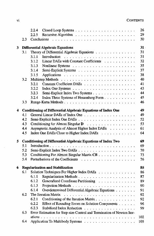
tems theory is the analysis of robots and mechanisms. Such systems are composed of connected bodies and are ideally suited for rnadelling as multibody systems. Figure 1.3 depiets a typkal robot. Simulation of the motion of a mul ti body system is useful for vari­ous problems of dynamic analysis. Of interest is particularly the motion of the multibody system, i.e. the positions, the veloeities and the accelerations, but also the internat forces under the influence of the extemally applied forces. Such dynamic simulations are an important part of computer aided design. They give the designer or engineer a powerful

1.2. MULTIBODY DYNAMICS AND FORMALISMS 3

Figure 1.3 Model of a robot arm

tooi to explore and predict, how real systems would behave under the influence of applied forces, by analysing mathematica! models without having to build expensive prototypes. This gives the designer orengineer the opportunity to analyse the mechanica! system and optimize its performance. For example one can evaluate the ride performance of a car and the ride comfort for its passengers. Another important area of applications is the crash safety field. In this area simulations are used for the reconstruction of actual acci­dents, for the anal ysis and the design of the crash response of vehicles, and f or the design of safety devices such as safety beits and air bags for example. Figure 1.2 depiets a crash safety simulation, which displays the response of a dummy in a frontal crash, where the dummy is restrained by an air bag and a three-point belt system. The human body model may be modelled by a system consisting of fifteen to thirty rigid bodies, while the model of the deformable air bag is described by a large number of elements in a fini te element (FEM) setting. The actual forces and accelerations found in simulations like that in Fig­ure 1.2 exhibit shocks and discontinuities. As a result, these kinds of complicated simu­lations require sophisticated simulation tools. This thesis deals with numerical methods for simulating such applications.

The rest of this chapter consists of four parts. In the following section an overview is given of the historie development of multibody system dynamics and the construction of general purpose multibody programs. Section 1.3 shows that the resulting equations of motion for large classes of multibody systems willlead to differentlal algebraic equa­tions (DAEs ), which also occur in other major application areas. First of all, a short his­torie overview ofDAEs is given. Next, some very importantcharacteristics ofDAEs are briefiy explained, showing that these kinds of equations are difficult to solve using nu­merical integration methods. The objectives of this thesis are explained in Section 1.4.

1.2 MULTffiODY DYNAMICS AND FORMALISMS

1.2.1 Bistory of Multibody Dynamics

The first person to formulate the equations to describe mul ti body systems for the human body was Fischer (1906) (cf. [26]), whomodelled the human body as a system ofthree

4 CHAPTER 1. SCOPE OF THE THESIS

coupled rigid bodies. However, he was unable to solve the resulting equations. Gener­ally, the motion of multibody systems is described by differentlal equations, often cou­pled with àlgebraic constraint equations that describe the interconnection between adja­cent bodies. These equations must be satisfied by the relative motion of the interacting bodies and the Lagrange multiplier associated with the aforementioned constraints. In classica! mechanics these equations are reduced toa system of ordinary differential equa­tions (ODEs), the so-called statespace representation or Lagrange equations of type two. In genera!, large displacements are possible and the descriptive equations are highly non­linear. The reduction to a state space representation may require strong simplifications of the mechanica! models. As a result, we can only formulate the governing equations by hand for very simple mechanica! systems and there are only a few mechanica! sys­tems that can be completely solved analytically. This gave rise to the need for reliable and efficient numerical methods for the simulation of mechanica! systems. That is why in the early sixties the first multibody formalisms were developed, ie. methods for the generation of the descriptive equations. There were two separate impulses for this devel­opment. The first was the increasing power offered by digital computers, and the other was the need for detailed analysis of mechanica! systems in the design of spacecraft and of high-speed mechanisms. The study of specific cases was started then and several spe­cial purpose programs were written. Towards 1965 increasing attention was paid to the construction of general purpose multibody computer programs that are capable of sirn­ulating very broad classes of multibody systems. Since then several of these multibody programs have been developed.

1.2.2 The Choice of a Set of Variables

While developing such multibody programs there are some very important issues that have to be considered. First, in the rnadelling process the choice of the set of variables used to represent the motion of the system is crucial. This set of variables should define the positions, the veloeities and the accelerations of the system in a unique way at each time. The most important types of coordinates are absolute coordinates, i.e. Cartesian coordinates, and relative coordinates or state variables. The absolute coordinates define the position and the velocity of a body with respect to an inertial reference frame. This results in a maximal set of Cartesian coordinates for each body. The relative variables represent the position and the velocity of a body in terms of relative motions between the interconnected bodies and result in a minimal set of variables. The choice of a set of variables is closely related to the formulation of the dynamics of the mechanica! system, which will be described in the next subsection.

1.2~3 The Choice of the Formulation of the Dynamics

Another important aspect is the choice of the formulation of the dynamics. The dy­narnic equations are based on the laws of Newton and Euler. For the development of multibody formalisros various methods for the generation of the equations of motion are used, i.e. Newton-Euler equations, Lagrange's equations of the first and secoud kind

1.2. MULTIBODY DYNAMICS AND FORMALISMS 5

and d' Alembert's principle of virtual work. All these formalisms lead to different, but equivalent, formulations of the equations of motion. The relative advantages or disad­vantages of the approaches depend upon the particular dynamic metbod being used, and the metbod used to organize the complex geometry. In general, one can determiné two approaches, viz. the augmentation method and the elimination method, depending on whether one wants to augment the constraint equations to the dynamic equations lead­ing to the so-called descriptor form or whether one wants to eliminate the constraints from these equations, resulting in a state space representation. In the first approach one chooses a set of absolute coordinates. As a result, this approach willlead to a maxi­mal number of descriptive equations, i.e. dynamic as well as constraint equations. How­ever, tbe generation of the resulting equations of motion will be rather simple in this approach. As an example, consider a double pendulum (cf. Figure 1.4) which is kept as a reference model during the whole thesis. This double pendulum is a compound

Figure 1.4 The double pendulum

of two coupled uniform rigid rods, denoted as bodies B1 and Bz, respectively, moving under the influence of gravity. The eentres of mass of Bt and Bz are M1 and Mz, re­spectively. Por this system the position of M1 is given by the absolute Cartesian co­ordinates x1 and y1 and the orientation of rod Bt is given by <fJl, and likewise for Bz by x2 , y2 and <pz. However, this system has only two degrees of freedom, viz. the rotation angles <p1 and <pz, because the system is constrained by the requirement that rod B1 has its pivot pin in 0 and that the pivot pin of rod B2 coincides with the pivot on the distal end of rod B1. This implies that the dynamic equations have to be augmented with con­straint equations, while unknown Lagrange multipliers account for the constraint loads. Hence, the resulting equations of motion ( which will be derived more in detail in Chap­ter 2) forma system of differential equations (i.e. the dynamic equations) tagether with algebraic equations (i.e. the constraint equations) and is therefore called a system of dif­ferential algebraic equations (DAEs).

Altematively, for the double pendulum shown in Figure 1.4 the rotation angles <(Jt

and <pz can be chosen as relative coordinates, resulting in a system of ODEs (this is elab­orated in Chapter 2). The second metbod uses relative variables. This minimal set of joint coordinates leads to fewer equations with higher complexity, since it is possible to eliminate constraint equations and constraint loads.

6 CHAPTER 1. SCOPE OF THE THESIS

1.2.4 Open Loop and Closed Loop Systems

Relative variables are especially effective for open loop systems where the bodies form tree configurations. These open loop systems appear naturally in the description of space­craft and robots (cf. Figure 1.3). The compound double pendulum of Figure 1.4 is an open loop system. The resulting equations of motionforma system ofnonlinear (ODEs).

Many mechanica! systems, however, are closed loop systems containing closed chains, implying that some elements of the multibody system are connected in more than one way. The treatment of this class of systems, however, is far more complicated than the treatment of open loop systems. Systems with closed ebains can be transformed into tree con:figuration by cutting selected joints (an idea developed by Wittenburg [84]), the so­called cut joints between bodies. This implies that the relative coordinates are not inde­pendent anymore, since they are subjecttothese additional cut joints. Consider a crank-

Figure 1.5 The crank-slider mechanism

slider mechanism as shown in Figure 1.5. This mechanism can be brought into tree con­figuration by cutting the joint constraining the distal end of Bz to move along the x-axis. Here, the rotation angles rp1 and rpz are not independent. Hence, the dynamic equations have to be augmented with a constraint equation that constrains the distal end of Bz to the x-axis, and again, Lagrange multipliers account for the constraint loads. Therefore, the resulting equations of motion form a system of DAEs.

1.2.5 Other Practical Aspects

Other important aspects in the simulation of multibody systems include the rednetion of computer time required for the simulation, which is most important in reai-time simu­lations, and the minimization of the amount of data storage, since realistic mechanica! models can be huge and very complex. Therefore, there is a growing interest in multi­body formalisros that have a high potentlal for parallel computation (cf. [6, 23]).

Another practical problem in the dynamic analysis of multibody systems is the oc­curance of discontinuities. These discontinuities appear in the modelling of e.g. crashes, hysteresis, dry friction and contact problems. The appearance of discontinuities cause severe problems during the numerical salution of such problems. An important require­ment for a multibody code is that it can deal with these discontinuities in a robust and efficient way.

1.3. ÜCCURRBNCE OF DIFFERENTlAL ALGBBRAIC EQUATIONS 7

Inthelast decade there has been a growing interest in the modelling of flexible bodies in multibody systems (cf. [16, 51-53]). The model of an air bag shown in Figure 1.2 is an example of such a flexible body. In the referred works flexibility is restricted to smal! deformations of bodies experiencing large displacements.

1.2.6 Multibódy Programs

As aresult of these observations, several general purpose multibody programs have been developed. These kinds of programs generate both the kinematic and dynamic equations, solely basedon input data descrihing the way the bodies are interconnected, the mechan­ica! and geometrical properties of the bodies and the interactions between them, tagether with the system state at the outset Afterwards they integrate the resulting equations of motion. A variety of powerful new algorithms that efficiently generate the highly nonlin­ear equations of motion of multibody systems bas been developed. This made it possi­bie to derive the governing equations for very complex and realistic mechanica! systems, even, so that very detailed roodels of machines and robots for example can be simulated.

Various methods are used in these multibody programs. Cartesian coordinate for­mulations are the basis for codes like ADAMS (cf. [15]) and DADS (cf. [80]), which are widely used in industry. They express the equations of motion in descriptor form and they result in a large set of highly sparse equations. Robers on ( cf. [72]) and Witten­burg ( cf. [84]) introduced graph theoretica! methods, with cut joint concepts that lead to spanning trees and a minimal set of generalized coordinates and constraint equations. These methods form the basis for all sorts of new computational formulations. They have led to the generation of recursive formalisms ( cf. [1, 5, 6, 49, 73, 79]) that build upon the topological relative coordinate foundation. These recursive formalisros generate the equations of motion in a very efficient way. The general multibody program MADYMO (cf. [58]) uses such a recursive formulation. It bas several features for crash analyses. MADYMO can be used to simulate the behaviour of crash-victims. Since it contains a finite element module, one can also study the interaction between the victims and the deformable vehicle structures as wellas the safety devices. This combination of a multi­body package and a finite element metbod is especially important when the interaction with highly deformable structures, like air bags, or vehicle interlor padding is simulated (cf. Figure 1.2).

1.3 OCCURRENCE OF DIFFERENTlAL ALGEBRAIC EQUATIONS

1.3.1 Bistorical Overview

Section 1.2 shows that, depending upon the particular dynamic metbod and the geomet­rie properties, the resulting equations of multibody systems are composed of DAEs or ODEs. DAEs also arise in many other application areas, including electrical networks, flows of incompressible fluids, control theory, robotics and chemica! reaction kinetics.

8 CHAPTER 1. SCOPE OF THE THESIS

One can think of DAEs as systems of differentlal equations coupled with constraining equations. The first paper on the numerical salution ofDAEs was written by Gear ( cf. [31]) in 1971. Particularly, the so-called backward differentlation formulae (BDF) (cf. Chap­ter 3) appeared to be effective for the salution of these systems. Only in the 1980's did the systematic study of numerical methods for the salution of DAEs begin and over the last few years there has been growing research activity in this area. Petzold ( cf. [ 65]) has shown that DAEs can differ substantially from ODEs, a fact that produces great difficul­ties for the numerical integration of DAEs. In fact, the numerical solutions of DAEs are far more difficult than the solutions of ODEs. Some DAEs can be solved numerically by methods developed for the salution of stiff ODEs, whereas other DAE systems can not be solved by such ODE sol vers. The research actlvities of the 1980' s contributed much to the understanding of the nature of DAEs. The most important results over these years were summarized in four interesting monographs [9,40,41,43]. They provide good in­sight into both the mathematica! structure of DAEs and the analysis of numerical meth­ods applied to DAEs.

1.3.2 Charaderistics of DAEs

As stated earlier, DAEs are difficult so solve numerically. To explain this briefly, consider some simple DAE systems:

x+y=u,

x-y=v,

where u and v are given forcing functions. The latter DAE has the following solution

x(t) =exp(-t)x(O) +exp(-t) I exp(s)(u(s) +v(s))ds,

y(t) =x(t) -v(t).

One observes that the solution is of the same form as for ODEs, i.e. the solution de­pends on the forcing terros themselves but oot on derivatives of them. Therefore, this DAE is called a DAE of index one. However, there is one difference with respect to ODEs, sirree the initia! value y(O) can not be chosen freely. It bas to satisfy the relation y(O) x(O) - v(O), whereas one may choose an arbitrary initia! value for x(O). In fact, this DAE will not exhibit any problems, except the usual ones in numerically solving ODEs. A somewhat more complicated DAE is given by the following system

x+y u,

X=V,

for given forcing functions u and v. It is obvious that this DAE bas the salution

X V,

y u-v.

1.4. 0BJECTIVES 9

Contrary to ODEs or DAEs of index one, the solution in this case depends on the first derivative of the forcing function v. Furthermore, both initia! valnes x{O) and y(O) can not be chosen freely. The index of this DAE is two and the system appears to be more difficult to solve numerically than the system of index one or a system of ODEs. Next, consider the DAE system

x+y=u,

y+z=v,

x=w,

for given functions u, v and w. The resulting solution is

x=w,

y=u-w,

z=v-u+w.

(1.1)

For this system the solution not only depends on the first derivative of the forcing func­tions, but even on the second derivative of the forcing function w. As a consequence, this DAE system has index three and it is even more difficult to solve numerically than the aforementioned index two system. In DAE theory the index concept gives a classifi­cation of DAEs. The index will characterize the numerical difficulty of a DAE.

Any textbook onmultibody systems (e.g. [45, 73, 84]) will show that the equations of motion for systems containing only kinematic constraints generally are of the following form

q=v, Mv+l/J!À =g,

O=l/J(q,t),

(1.2)

where q denotes the generalized positions, v denotes the generalized veloeities and M is the generalized mass matrix that is positive definite. The applied and outer forces are given by g. The matrixl/Jq := = is the Jacobian of the constraint equations. The Lagrange multipliers À account for the constraint loads. Camparing the index three DAB ( 1.1) in the variables [x, y, z]T to equation (1.2) in the variables [q r, vT, À T]T, it is easy to see (by identifying x with q, y with v and z with À) that (1.2) is a DAE of index three. As a consequence, they are very difficult to solve numerically.

1.4 OBJECTIVES

The main reason for writing this thesis was to develop a reliable and efficient numerical metbod for approximating the dynamics of multibody systems with closed loops. Multi­body dynamics often give rise to DAEs with forcing functions exhibiting discontinuities in the form of finite jumps, either in the function itself or in some derivatives of it. There­fore, the metbod should adapt to these discontinuities.

10 CHAPTER 1. SCOPE OF THE THESIS

To accomplish our goals we first have to study the structure of the dynamic equations of multibody systems and more especially for closed loop systems. Since they generally constitute a system of DAEs, a thorough study of such equations is needed. An impor­tant topic in DAE theory is the conditioning of DAEs, i.e. the sensitivity of the equations to small changes in the system. The conditioning of a DAE can be considered by de­riving a statespace equation for tbe DAE, resulting in an ODE. The conditioning of this state space ODE can be studied as in standard theory for ODEs then. However, for DAEs some important quantities have to be introduced that are not neededinODE theory. This is due to the differentnature of such equations compared to ODEs. InSection 1.3 the im­portance of the index concept of a DAE was already pointed out. It appears that index v DAEs may effectively behave like DAEs of index higher than v, i.e. DAEs of index one may behave as complicated as DAEs of index two or higher for examle. Unfortunately, it appears that in tbe case of DAEs of higher index perturbations of the equations, espe­cially in some coefficients, may lead to large perturbations in the solution. This might cause severe problems during the numerical salution of such systems. In fact, it would be easier to solve the associated reduced higher index problem. We already pointed out tbat the numerical salution of DAEs of a higher index is rather difficult. In general tbe inte­gration of such problems by metbods for tbe salution of stiff ODEs is not possible, since most of them are only convergent for index one DAEs and a loss of the approximation order for the algebraic variables occurs. BDF methods, however, are shown to converge forsome classes of DAEs of a higher index, such as Hessenberg forms (cf. Chapter 3) which is tbe general form of the equations of motion for multibody systems, although they exhibit problems due to ill-conditioning of tbe iteration matrix, and the orderand step-size control may fail. Reducing the index to one by differentlation of tbe constraints yields a problem that can be integrated by such a numerical metbod. A major disadvan­tage of this approach is tbat the numerical salution will drift away from the constraints, since it does not satisfy the original constraints. Therefore a numerical metbod has to be developed, tbat minimizes tbis drift-off effect, such that higher index DAEs, generated in e.g. multibody dynamics, can be integrated numerically.

As stated in tbe objectives tbe numerical metbod for tbe salution of the equations of motion of mechanica! systems should solve systems exhibiting dîscontinuities, since in multibody dynamics discontinuities occur very often, e.g. in tbe rnadelling of impact ( cf. also Figure 1.2), hysteresis, Coulomb friction, etc. The lack of smootbness, due to tbe discontinuities, is tbe cause of numerical difficulties, since tbe required differentiabil­ity in tbe convergence analysis is not present. As a consequence, tbe step-size selection of a numerical metbod may break down and tbere is no safe local error estimation any­more. During tbe passage of tbe singularity, the metbod may become very inefficient because of repeated step-size reductions. These problems can be circumvented by the use of switching functions that determine whether the integrator passes a discontinuity. These functions can be used either to localize the singularity or to reduce the step-size of tbe numerical metbod. Then the integration is restarted at tbe singularity, or it is contin­ued with reduced order and step-size. In tbis way the discontinuity is handled in a more efficient way.

1.5. CONTENTSOF THIS THESIS 11

1.5 CONTENTS OF THIS THESIS

In this section we briefly outline the contents of this thesis. In Chapter 2 the mathematical formu1ation descrihing the kinetics and dynamics of

multibody systems is derived. The laws of Newton and Euler form the basis for the dynamic equations. From these basic concepts the dynamic equations for mechanical systems can be generated. The constraint equations, descrihing the interconnections be­tween several elements <>f the mu1tibody system, can be incorporated in two different ways. In the augmentation method the constraints are added to the dynamic equations. Application of the method of Lagrange multipliers implies that the constraining forces are represented by the unknown Lagrange multipliers. This augmentation metbod re­su1ts in the descriptor form of the equations of motion. The resulting system is a system of DAEs. In the elimination method, one chooses a set of relative coordinates descrih­ing the motionsof bodies relative toeach other. U se of this set of so-called state vari­ables eliminates both the constraint equations and the associated forces, yielding the state space formu1ation forming a set of ODEs. However, this metbod only generates a sys­tem of ODEs for <>pen loop systems (cf. Figure 1.4). The generation of these equations can he performed in a very elegant and efficient way using a recursive formulation of the mu1tibody system. In cases where the mu1tibody system contains closed loops, one can also use this recursive method to generate the dynamic equation. For this type of problem one has to cut some joints in order to retrieve an open loop system. Thereby one introduces cut joints. This implies that the resulting equations of motion now form a system of DAEs, since the relative coordinates are not independent anymore because of the cut joints that have to he accounted for.

Chapter 3 focuses on the basic theory of DAEs. It explains the index concept and gives some related definitions of the index, such as the differentlal index and the pertur­bation index. The index gives a classification ofDAEs and plays a key role in the study of existence and uniqueness of solutions of DAEs. In a way, the index indicates how much a DAE dîffers from anODE. A characterization ofDAEs regarding their index and their structure is given. In addition, the numerical salution of DAEs by direct methods, such as multistep and Runge-Kutta methods is studied. In general, only DAEs of index one can be solved directly. It appears that the higher the index, the greater the numerical dif­ficulties.

The objective of Chapter 4 is to study the question of conditioning of DAEs of index one. Mter briefly consictering generallinear DAEs the more transparent case of semi­explicit linear index one DAEs is studied. In this manoer we can analyse the influence of perturbations of the equations on the solution, which obviously is very important for the numerical salution of DAEs. We will show that index one DAEs may be close to a DAE of a higher index, i.e. the salution of such index one systems effectively behaves like the salution of a higher index DAE. Consequently, such equations generally are ill­posed and are therefore difficu1t to solve numerically. These kinds of systems practically behave as if they were of an index higher than two, meaning that it is important to know the effective index of the DAE.

Chapter 5 deals with the conditioning of index two DAEs and explains their salution

12 CHAPTER 1. SCOPE OF THE THESIS

behaviour. We will show that index two DAEs may behave like DAEs of index three or higher. Por such systems it will appear to be very interesting to consicter perturbations of the coefficients.

The subject of Chapter 6 is the study of solution methods for the equations of mo­tion for multibody dynamics. Standard methods for the numerical solution of ODEs are generally not suited for the solution of DAEs of index two or higher. Lowering the in­dex by differentiation will not help, since index rednetion gives rise to drift, which can make the numerical solution completely useless. Therefore, numeric.al methods have to be developed that alleviate this drift. The condition number of the iteration matrix of such methods is studied in detail, both for well-conditioned systems as well as for sys­tems close to DAEs of higher index. Numerical methods applied to the latter type of problems can suffer from problems with respect to stability for example. Luckily how­ever, BDF methods will exhibit these problems to a smaller extent. We will show how this sort of problems can be reduced by a partienlar stabilization technique. This will be demonstraled by some numerical examples. Next, applications of multibody systems are presented. Examples of ill-conditioned multibody systems will be shown and the stabi­lization technique of the previous chapter will be applied.

Shocks and discontinuities frequently occur in the dynamics of multibody systems and cause great difficulties for the numerical solution, i.e. salution methods for ODEs as well as for DAEs may become very inefficient or may even fail due to the presence of discontinuities. In Chapter 7 attention will be paid to the numerical simulation of such problems in order to develop methods suitable for the efficient and robust simulation of discontinuons differential equations. Applications of discontinuons mechanical systems, i.e. systems exhibiting impacts, hysteresis and Coulomb friction for example, are pre­sented.

In Chapter 8 the achievements in this study will be reviewed in view of the objec­tives stated inSection 1.4. We conclude with a brief discussion and some suggestions for further research and development.

2 MULTIBODY SYSTEMS

Equations of motion for multibody systems may be obtained by various formalisms. The basic approaches for generating these equations are tbe augmentation metbod and tbe eliminationmethod. The augmentation metbod generates tbe descriptorform oftbe equa­tions of motion and results in a system of differentlal algebraic equations. For open loop systems a set of ordinary differentlal equations is yielded by tbe elimination metbod. These metbods are reviewed. Recursive methods for tbe generation of tbe equations of motion for mechanical systems significantly rednee computer time needed for generating tbe dy­namic equations. A recursive formulation for obtaining tbe equations of motion, botb for open loop systems and for closed loop systems, is given.

2.1 BASIC CONCEPTS FOR GENERATION OF EQUATIONS OF MOTION

Multibody simulation programs genera te the multibody system equations from a descrip­tion of the system elements and the system topology. These equations can he generated in various farms. Earlier workin obtaining equations of motion for mechanica! systems can generally be divided into two basic approaches, viz. the augmentation metbod and the elimination method. In this section, methods for the generation of mul ti body system equations are discussed.

2.1.1 Primitive Equations of Motion

Following the concepts of classica! mechanics, we assume that there is an inertial frame, such that the equations of motion, basedon Newton's secoud axiom for translational mo­tions and Euler's axiom of moment of momentum, hold fora system of n rigid bodies, denoted by B; (i= I, 2, ... , n). Let m; be the mass of body B; and J; be the inertia ma­trix of B; with respect to its centre ofmass. The absolute position vector ofthe centraid

14 CHAPTER 2. MULTIBODY SYSTEMS

of B; is denoted by r; and the absolute angular velocity of B; is given by á>;. Let f; de­note the total force acting upon B; and n; denote the resultant moment on body B; with respect to its centroid. With respect to the inertial frame, the equations read

M{v; = g;, i 1, 2, ... , n, (2.1)

where M; := [ 61 ~] denotes the generalized mass matrix, v; := [~;]is the global velocity

of body B; and g; := [ IJi-(l)j~(JJt»;) J is the generalized loatfl vector. This can be illustrated by the following

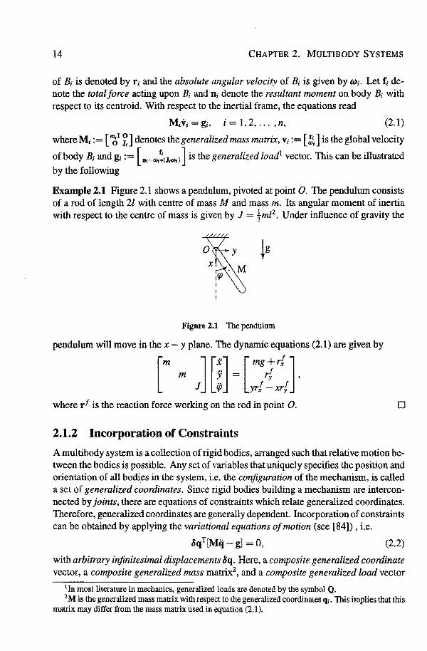
Example 2.1 Figure 2.1 shows a pendulum, pivoted at point 0. The pendulum consists of a rod of length 2l with centre of mass M and mass m. lts angular moment of inertia with respect to the centre of mass is given by J = %ml2• Under influence of gravity the

Figure 2.1 The pendulum

pendulum will move in the x - y plane. The dynamic equations (2.1) are given by

[m ] [x] [mg+r[] m y= rf ,

J (/J · yr[ -xr{ where rf is the reaction force working on the rod in point 0. 0

2.1.2 Incorporation of Constraints

A multibody system is a collection of rigid bodies, arranged such that relative motion be­tween the bodies is possible. Any set of variables that uniquely specifies the position and orientation of all bodies in the system, i.e. the conjiguration of the mechanism, is called a set of generalized coordinates. Since rigid bodies building a mechanism are intercon­neeled by joints, there are equations of constraints which relate generalized coordinates. Therefore, generalized coordinates are generally dependent Incorporation of constraints can be obtained by applying the variational equations of motion (see [84]), i.e.

&qT[Mq g] 0, (2.2)

with arbitrary infinitesimal displacements 8q. Here, a composite generalized coordinate vector, a composite generalized mass matrix2, and a composite generalized load vector

1 In most literature in mechanics, generalized loads are denoted by the symbol Q. 2M is the generalized mass matrix with respect to the generalized coordinates q;. This implies that this

matrix may differ from the mass matrix used in equation (2.1 ).

2.1. BASIC CONCEPTS FOR GENERATION OF EQUATIONS OF MOTION 15

are defined by

q := (qÎ, qi, ... 'q~]T,

M := diag(Mt, Mz, · · · , Mn) and

. [ T T TjT g .= gt • gz • · · · • gn •

respectivel y. The loads in equation (2.2) include the unknown generalized constraint loads, which

have to be exerted by the coustraints in order to compel the system to fulfill the kinematic conditions. Allloads other than constraint loads are called generalized applied loads. These are either explicitly known or can be formulated explicitly in terms of the gener­alized coordinates. Let the generalized loads g be divided into the generalized applied loads ft and the generalized constraint loads ge, i.e. g g' +ge. Using the preceding notation, equation (2.2) may be expressed as

(2.3)

for arbitrary &q. Here, &qTg: is the so-called total virtual workof constraint loads acting on all bodies in the system. By Newton' s law of action and reaction, eaustraint loads act perpendicular to contact surfaces (if there occurs no friction in kinematic joints) and oc­cur in pairs of equal magnitude and opposite direction. Aso-called virtual displacement or kinematically admissible displacement of a system refers to a change in the contigu­ration of the system as the result of any arbitrary infinitesimal change of the coordinates q, consistent with the loads and the constraints imposed on the system at the given in­stant t. Thus restricting attention to virtual displacements, the total virtual work of all the constraint loads in the system is zero, i.e. 8Wc = &q r ge = 0, the so-called principle ofvirtual work. As a result, the constrained variational equations of motion may now be written as

(2.4)

for all virtual displacements 8q. The latter equation is the so-called d'Alembert's prin­ciple of virtual work. We have achieved that the constraint loads no Jonger appear, and the superscript a can now be dropped without ambiguity.

At this point, the well-known classification of constraints into holonomic and non­holonomic becomes important. A constraint is called holanomie if the constraint equa­tions can be expressed as equatious connecting the coordinates of the bodies in the fol­lowingform

t/>(q,t) =0, (2.5)

whereas the nonholanomie constraints can be expressed as

1/l(q, q, t) = 0, (2.6)

16 CHAPTER 2. MULTIBODY SYSTEMS

i.e. they depend on q explicitly. For these nonholonomic constraints it is, by definition, impossible to set up a number of equations connecting the coordinates and the time like equation (2.5), since otherwise they would represem holonomic constraints. The sim­plest examples of nonholanomie systems occur in problems dealing with the rolling mo­tion of one body upon another. In addition, nonholonomic constraints naturally occur during the stick phase of systems exhibiting Coulomb friction (see Section 7 .3) In most practical problems t is a linear function of generalized veloeities so that equation (2.6) can be written in the form

lfr(q, q, t) = P(q, t)q + p(q, t) 0. (2.7)

For holonomic constraints, the varlation of tP caused by a varlation of the generalized coordinates (with time frozen) is zero, whence we conetude

tPqÓq = 0, (2.8)

where t/Jq := = is the Jacobian of tiJ with respect to q. From the nonholonomic con­straints (2. 7) it follows ( cf. [84]) that öq should satisfy the relationship

Póq =0. (2.9)

Hence, equation (2.4) should hold for all virtual displacements öq satisfying the equa­tions (2.8) and (2.9).

Applying the methad of Lagrange multipliers (cf. [45, 84]) to equation (2.4) results in

(2.10)

for arbitrary óq. In this equation À contains the unknownLagrange multipliers, account­ing forthe unknownconstraintloads, and H := [ f,pTf. Sinceóqis arbitraryin (2.10), we obtain the Lagrange multiplier form of the equations of motion

In the remainder of this chapter, however, we will consicter holonomic constraints only. So, the equations of motion yield

Mq +t/J~À = g. (2.11)

2.1.3 Augmentation Method

Applying the approach of the previous Subsection, we derived the Lagrange multiplier form of the equations of motion (2.11 ). In JR.3 this system represents a set of 6n equations in the 6n unknown generalized coordinates q and the nh unknown Lagrange multipliers À, where nh is the number of holanomie constraints.

2.1. BASIC CONCEPTS FOR GENERATION OF EQUATIONS OF MOTION 17

In order to describe the motions of the complete system, equation (2.11) has to be augmented by the position constraints (2.5), the velocity constraints and the acceler­ation constraints. The velocity constraints are obtained by differentlating the position constraints (2.5) with respect to time, giving

t/>qq -tf>t =:V. (2.12)

Differentiatingthe position constraints once more one obtains the acceleration constraints

(2.13)

The equations (2.12) and (2.13) tagether with (2.11) and (2.5) camprise the complete set of constrained equations of motion for the system. Combining equations (2.11) and (2.13) results in

[~ ~~] [1] = [;]. (2.14)

Since, the mass matrix M is positive definite, this system has a unique solution for the accelerations and the Lagrange multipliers if t/>q has full row rank. Hence, the equations of motion are salvabie if the eaustraint equations are independent. The above metbod of augmenting the dynamic equations with the eaustraint equations is called the augmen­tation method.

This metbod keeps the unknown eaustraint farces, takeninto account by the Lagrange multipliers, in the equations of motion. Augmenting equation (2.11) by one of the eau­straint equations (2.5), (2.12) or (2.13) gives a set of DAEs. This metbod yields the so­called descriptor form of the mechanica! system (see [57]). These equations are called Lagrange's equations of type one and are an often used basis for multibody formalisms, e.g. [46,63,64].

Example 2.2 The kinematic eaustraint equations for the pendulum of Example 2.1 read

.t..( ) = [x l c~s lp] = 0 'I' q y -/ Slnlp '

where we obtain the generalized coordinate vector q [x, y, lp]1 . The velocity and ac­celeration constraints are

. [i+ fep Sin lp] O t/>qq = y -lij) cos lp

and

.t..qq·· [.i + 191 sin lp] . . [lq} cos lp] 'I' ji -[9)COSlp = -(t/>qq)qq =- flj}2 SÎUlp .

Applying the metbod of Lagrange multipliers, we obtain

[ m m ] [;] + [ ~ ~ ] [~1 ] = [~g]. J 9) fSÎUlp -[COSlp

2 0

Together, these last two equations form the system of equations (2.14). 0

18 CHAPTER 2. MULTIBODY SYSTEMS

This approach has the advantage of generality and results in relatively simp Ie equations, which can be generated efficiently. The disadvantages are the description by a set of DAEs and the large number of descriptive equations. Commercial codes like ADAMS (cf. [15]) or DADS (cf. [80]) use this metbod to generate the system equations.

2.1.4 Elimination Metbod

Another route for deriving the equations of motion is the elimination method. In this approach the system motion is represented by a minimal set of relative varlab les, called the state variables. The goal of this metbod is to eliminate both the constraint equations and the constraintloads. Therefore, the system equations are reduced toa so-called state space representation (cf. [73]), i.e. a set of ODEs. The constraint loads may then be computed from a second set of equations. We discuss this metbod briefly below.

The kinematics of a system of bocties is described by a set of relative coordinates. For that reason, the motion of a particular body in the system is defined with respect to an adjacent body, which motion has previously been defined according to the topological ordering of all bodies in the system. Note, that in the augmentation metbod one uses a global description, i.e. motions of all bodies in the system are represented with respect to an inertial coordinate frame.

Consider two bodies B and B' interconnected by the joint with index d, say. As a result, the relative motion of the two bodies is constrained by nd constraint equations. On that ground, the number of degrees of freedom of motion of the bodies relative to each other is

(2.15)

So, the motion of the bodies relative to each other can be described by independent rela­tive joint coordinates, denoted by qd, qd E /Rn t. These coordinates are required to satisfy the constraint equations automatically. Applying the varlational equations of motion ( cf. Subsection 2. 1.2) forthese two bodies, a virtual varlation óqd may not violate the kine­matic constraints between bodies Band B'. Since relative joint coordinates automat­ically satisfy the constraints, óqd in equation (2.4) is arbitrary. So, it is not necessary to introduce Lagrange multipliers as in equation (2.1 0). We shall elaborate this in Sec­ti on 2.2.3.

Example 2.3 The pendulum of example 2.1 has only one degree of freedom, because it is a planar system. Therefore, its motion can bedescribed as a function of the statespace variabie q;. Varlation of the generalized coordinates q gives

[~x] [-l sinq;] óq = :; = . lc~sq; oq;.

2.2. RECURSIVB PORMULATION FOR CONSTRAINBD MBCHANICAL SYSTBMS 19

Using this expression for the virtual displacementsin the principle of virtual work (2.4), we obtain the dynamic equations for the pendulum

tml~ + mgsin.p 0,

where the constraint forces have been eliminated. 0

This procedure can be repeated for the entire multibody system. Por so-called open loop systems, i.e. systems in which all bodies are connected in a unique way, this results in a system of ODEs. In Figure 2.2 an open loop system is shown with ten bodies linked to­gether. However, difficulties occur when closed loops appear in the system. In that case

Figure 2.2 An open loop system consisting of ten bodies

the relative (joint) coordinates are not independent anymore, because two bodies can be connected in more than one way. Wittenburg ( cf. [84]) developed the idea of opening the closed loop, by cutting chosen joints, to form an open loop system. The opened system is called the reduced system. First, only this reduced system will be considered. Later, all constraints and all constraint loads which have been ignored in the process of generat­ing the reduced system have to be re-introduced. The now re-introduced constraint loads are provided by adding Lagrange multipliers to the equations of motion. In this way, the original closed loop system is reformulated. Relative description makes recursive for­mulation possible (cf. [5, 6, 73]). Within the context of mul ti body dynamics, a recursive formulation is a procedure in which elementary relationships, going for an arbitrary pair of contiguons bodies as part of a system of bodies, can be used all along the system. This can be used to generate the kinematic equations and the system matrices in the dynamic equations in a very efficient way.

2.2 RECURSIVE FORMULATION FOR CONSTRAINED MECHANICAL SYSTEMS

In this section, a recursive formulation of the equations of motion of spatially constrained mechanica! systems is derived. Before explaining the recursive method, we introduce in Subsection 2.2.1 the concept of body conneetion arrays for descrihing the way the rigid bodies are linked together by joints. Kinematics of an elementary system of two bodies coupled by an arbitrary joint is discussed in Subsection 2.2.2. The motion of one body

20 CHAPTER 2. MULTIBODY SYSTEMS

is expressed in terms of the motion of the adjacent body and the relative motion between the bodies due to the joint. Afterwards, in Subsection 2.2.3, the dynamics for a single chain, consisting of such elementary systems, is derived. Using a variational form of the dynamic equations, contributions to the mass matrices and load veetors of the lower num­bered bocties from all the connected higher numbered bocties are derived. This procedure is repeated for general open loop systems in Subsection 2.2.3 and a recursive algorithm is developed to rednee the equations of motion to a base body. In Subsection 2.2.4 this algorithm is extended to closed loop systems.

The workof Bae and Hang (cf. [5, 6]) is the basis for this section. Roberson and Schwertassek ( cf. [73]) obtained the same relations, however, their denvation is different. They applied the concept of modes of motion and corresponding generalized loads, while Bae and Haug used the variational form of the system equations.

2.2.1 Topology

A multibody system can be very complex and built up of many bocties and many joints. To create a computer oriented multibody formalism, one must devise a data structure descrihing the system topology. One can introduce aso-called system graph (see [84]), which represents the connectivity of the mechanica! system. However, the use of body conneetion arrays ( cf. [ 50]) provides a more elegant way to describe the topological rep­resentation of systems with a tree structure.

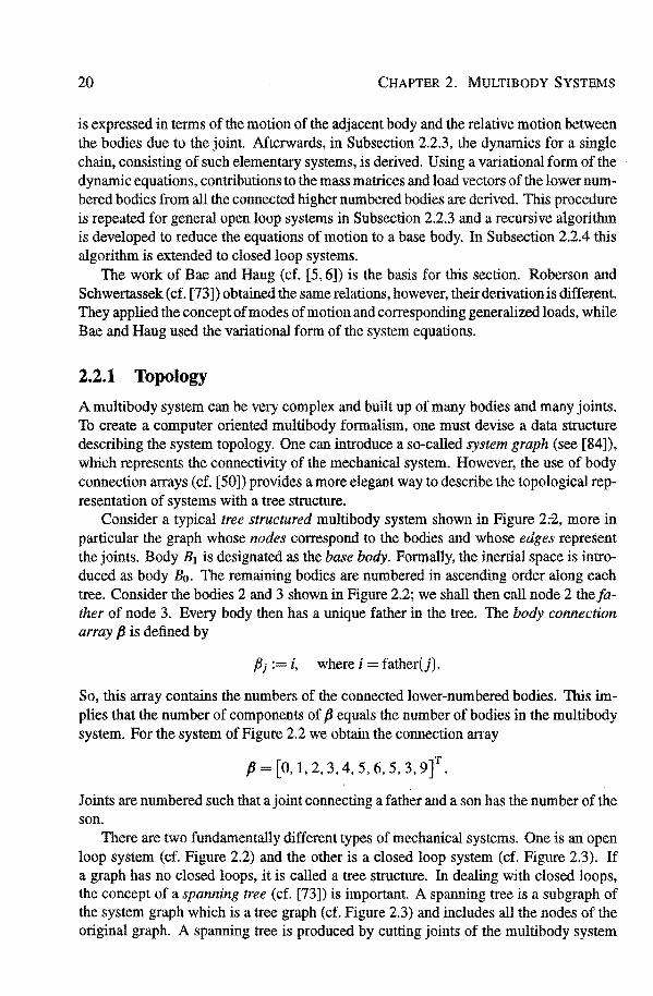
Consicter a typical tree structured multibody system shown in Figure 2;2, more in partienlar the graph whose nodes correspond to the bodies and whose edges represent the joints. Body B1 is designated as the base body. Formally, the inertial space is intro­doeed as body B0 • The remaining bodies are numbered in ascencting order along each tree. Consider the bocties 2 and 3 shown in Figure 2.2; we shall then call node 2 the fa­ther of node 3. Every body then has a unique father in the tree. The body conneetion array fJ is defined by

/3i i, where i= father(j).

So, this array contains the numbers of the connected lower-numbered bodies. This im­plies that the number of components of fJ equals the number of bocties in the multibody system. For the system of Figure 2.2 we obtain the conneetion array

{J = [0, 1, 2, 3, 4, 5, 6, 5, 3, 9]T.

Joints are numbered such that a joint connecting a father and a son has the number of the son.

There are two fundamentally different types of mechanica! systems. One is an open loop system (cf. Figure 2.2) and the other is a closed loop system (cf. Figure 2.3). If a graph bas no closed loops, it is called a tree structure. In dealing with closed loops, the concept of a spanning tree (cf. [73]) is important. A spanning tree is a subgraphof the system graph which is a tree graph (cf. Figure 2.3) and includes all the nodes of the original graph. A spanning tree is produced by cutting joints of the multibody system

2.2. RECURSIVE PORMULATION FOR CONSTRAINED MECHANICAL SYSTEMS 21

. . Yl ' .

/ / ,. ·'

~~

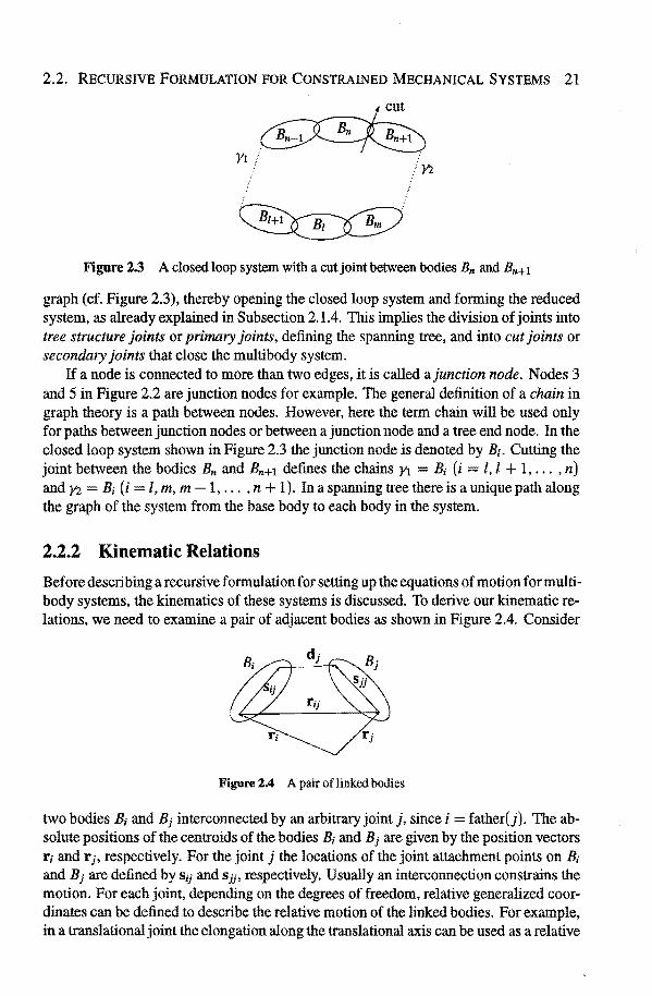
Figure 2.3 A closed loop system with a cut joint between bodies Bn and Bn+ 1

graph (cf. Pigure 2.3), thereby opening the closed loop system and forming the reduced system, as already explained in Subsection 2.1.4. This implies the division of joints into tree structure joints or primary joints, defining the spanning tree, and into cut joints or secondary joints that close the mul ti body system.

If a node is connected to more than two edges, it is called ajunetion node. Nodes 3 and 5 in Pi gure 2.2 are junction nodes for example. The general definition of a chain in graph theory is a path between nodes. However, here the term chain will be used only for paths between junction nodes or between a junction node and a tree end node. In the closed loop system shown in Figure 2.3 the junction node is denoted by B1• Cutting the joint between the bodies Bn and Bn+t defines the chains Yt = Bi (i l, l + 1, ... , n) and Yl Bi (i l, m, m - 1, . . . , n + 1). In a spanning tree there is a unique path along the graph of the system from the base body to each body in the system.

2.2.2 Kinematic Relations

Before descrihing a recursive formulationfor setting up the equations of motion for multi­body systems, the kinematics of these systems is discussed. To derive our kinematic re­lations, we need to examine a pair of adjacent bodies as shown in Figure 2.4. Consicter

Figure 2.4 A pair of linked bodies

two bodies Bi and B1 interconnected by an arbitrary joint j, since i = father{j). The ab­solute positions of the centroids of the bodies Bi and B1 are given by the position veetors ri and r 1, respectively. For the joint j the locations of the joint attachment points on B1

and B1 are defined by s;1 and s11 , respectively. Usually an interconnection constrains the motion. Por each joint, depending on the degrees of freedom, relative generalized coor­dinates can be defined to describe the relative motion of the linked bodies. Por example, in a translational joint the elangation along the translational axis can be used as a relative

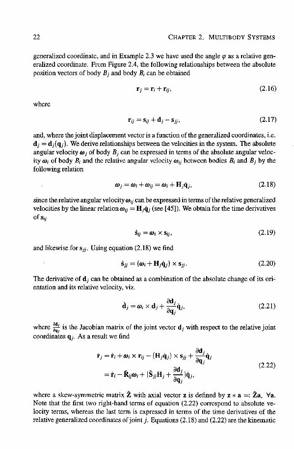
22 CHAPTER 2. MULTIBODY SYSTEMS

generalized coordinate, and in Example 2.3 we have used the angle ({J as a relative gen­eralized coordinate. From Figure 2.4, the following relationships between the absolute position veetors of body Bi and body B; can be obtained

(2.16)

where

(2.17)

and, where the joint displacement vector is a function of the generalized coordinates, i.e. di = di ( q;). We derive relationships between the veloeities in the system. The absolute angular velocity (J) i of body Bi can be expressed in terms of the absolute angular veloc­ity (J); of body B; and the relative angular velocity (J);i between bodies B; and Bi by the following relation

(2.18)

since the relative angular velocity (J);i can be expressed in terms of the relative generalized veloeities by the linear relation (J);i = Hj('J.; (see [ 45]). We obtain for the time derivatives of s;i

(2.19)

and likewise for sii· Using equation (2.18) we find

(2.20)

The derivative of di can be obtained as a combination of the absolute change of its ori­entation and its relative velocity, viz.

. adi d· =(I)· x d· + -q·. ' , ' a ,, q;

(2.21)

where ~ is the Jacobian matrix of the joint vector di with respect to the relative joint coordinates q;. As aresult we find

(2.22)

where a skew-symmetric matrix Z with axial vector z is defined by z * a =: Za, Va. Note that the first two right-hand terms of equation (2.22) correspond to absolute ve­locity terms, whereas the last term is expressed in terms of the time derivatives of the relative generalized coordinates of joint j. Equations (2.18) and (2.22) are the kinematic

2.2. RBCURSIVB PORMULATION FOR CONSTRAINBD MBCHANICAL SYSTBMS 23

equations relating absolute veloeities and relative velocities. Defining V i [!ti] , equa­tions (2.18) and (2.22) can be composed as

Vj = AjVj + Bjqj. (2.23)

where

[I -Rï]

Ai:= 0 I 1 and B1 [

- ad·] s .. u.+ ::::L JJ J ilqj

Hi . (2.24)

Por the denvation of the dynarnic equations in Subsection 2.2.3 we will use the varia­tional form of the system equations, for which we need expressions for the virtual dis­placements. Analogously to the denvation of the velocity equation (2.23) the virtual dis­placement equation (2.25) can be derived by replacing the time derivative by the varlation operator (see [ 45]), i.e.

(2.25)

with

ÓUj := [:~], (2.26)

where 6ri and 6Tti denote virtual translation and virtual rotation, respectively, and öq1 denotes virtual relative coordinates.

The matrix form of acceleration relations can be obtained by differentiation of equa­tion (2.23), i.e.

(2.27)

where

(2.28)

A·- J . [0 -i·] J- 0 0 (2.29)

The matrices A 1 and À 1 are independent of joint type, while B 1 and Bi depend upon the joint type and its relative coordinates. Equations (2.23), (2.25) and (2.27) are the recursive kinematic relations. The metbod described above shall be demonstrated on a simple example.

Example 2.4 Consicter a compound penduturn shown in Figure 1.4. where the bodies B1

and B2 have lengtbs 2l1 and 2[z, respectively. The relative joint coordinates are q1 = q;1

and qz = q;2• The position of the centre of mass of rod Bt is given by

rt = [l1 C?SCfJt]. ft StnC(Jt

(2.30)

24 CHAPTER 2. MULTIBODY SYSTEMS

The position of the centraid of rod B2 can be expressed as

[2lt COS(/Jt + lz COS((/Jt + ({Jz)] 2lt sin (/)1 + [z sin ( (/Jt + rpz) ·

(2.31)

Denote the inertial frame as body Bo, implying that vo = 0 and lûo = 0. Since Ht 1. d 0 d [ -11 COS<Pt] fi d

1 = an Sll -lt sin<Pt ' we n

Therefore, for rod B1 the following kinematic relations hold

Vt = Bt èt1. Vt = Bt iit + Bt «it and &ut Bt&qt. (2.32)

Therefore, the kinematic relations for veloei ties, accelerations and virtual displacements of Bz are

vz = AzVt + BzèJz, vz = Azv1 + Bziiz + Cz and &uz = AzÖUt + Bz&qz, (2.33)

respectively. Note that differentlating (2.30) and (2.31) with respect to time and aug­menting them with the rotational veloeities results in the same relations. 0

2.2.3 Open Loop Systems

In practice, open loop multibody systems appear less frequently than systems with closed chains. However, there are two reasans to treat this class of systems first. One reason is the greater simplicity of tlte mathematica! description of the interconnection structure and of the kinematics. The second reason is that, by cutting joints, the equations of roo­tion for a system with closed ebains can be obtained from the reduced system by intro­duetion of Lagrange multipliers as explained in Subsection 2.1.4. Cutting joints results in a tree structure mechanism only consisting of chains. We employ the recursive for­mulation, developed in Subsection 2.2.2, toa typical chain y (cf. Figure 2.5), beginning at a junction node l and proceeding to a tree end node n. The variational equations of motion for chain y are reduced to equations for a single body, viz. the junction body B1•

The variational equations of motion for the whole chain y ( cf. (2.4)) are

n

L &ui[Mtv; - ~] = 0, (2.34) i=l

2.2. RECURSIVE PORMULATION FOR CONSTRAINED MECHANICAL SYSTEMS 25

·········~

Figure 2.5 A typical chain y

whereciu;, i= l, l + 1, ... , n, are kinematically admissible for the constraints between the bodies B1 to Bn and any other constraints that may act on the junction body B1. Note that M; is defined as in Subsection 2.1.1. Repeated usage of the kinematic relations (2.25) and (2.27) between bodies the Bi and Bj-1 tagether with the joint coordinates q;, since j- 1 = father(j), leads to the recursive equations of motion for B1 (see Appendix A for a detailed derivation)

(2.35)

Here, 8u1 is kinematically admissible for all extemal constraints that act on the junction body B1. The recursive mass matrix Mj and the recursive load vector ~i for chain y are defined in Appendix A.

For more general open loop systems this procedure can be repeated for each chain (see [81] for an elaboration). The recursive mass matrices and load veetors of all chains, originating from the same junction body, are added together. The successive reduction process can be repeated all along the rest of the tree structure until one reaches the base body B1• It resu1ts in the variational equations of motion for B1, i.e.

(2.36)

for the whole tree -r. Now, 8u1 is kinematically admissible for the kinematic constraint between the base body B1 and inertial space, regardedas B0 (see Subsection 2.2.1). Since Bo has constant position, the position of body B1 relative to inertial space can be repre­sented by joint coordinates between B1 and Bo, just lik:e any other arbitrary joint between two adjacent bodies B; and Bj. The advantage of this procedure (cf. [76]) is that the in­troduction of Lagrange multipliers (as in [5]) is nat needed. Therefore, it provides the advantage of maintaining a system of ODEs and avoids having to solve a system ofDAEs as in [5].

The basic advantage of this process is the fact that the dynamic equations are gen­erated in explicit farm (see equations (A.2) and (A.6) in Appendix A) with a number of operations, which increases only linearly with the number n of the system bodies. There­fore, they are called O(n)-fonnulations (cf. [74]). Besides, the small dimension of the matrices that have to be inverted to obtain these joint accelerations (cf. (A.2) and (A.6)) is advantageous. For open loop systems this reduction process can be explained by the following

Example 2.5 For the double pendulum of Figure 1.4 the unreduced equations of motion read

(2.37)

26 CHAPTER 2. MULTIBODY SYSTEMS

where

[m· ] [m·g] Mi=

1

~ J; and g;= ~ .

Substitution of (2.33) into (2.37) results in

&ui{Mtirt -gt) +(&ui AI +&qiBIJ(Mz(Aivt +Bzêiz +cz) -gz) 0.

Since &q2 is arbitrary, we find

tiz = ih = -(BiMzBz)-1Bi{Mz(AzVt + Cz)- gz}. (2.38)

This can be rewritten as

(mzJi + ]z)(~t + ~z) + 2mzlth(~t COS<flz + cpÎsinq;z) + mzg/z sin(<Pt + <Pz) = 0.

Substitution of (2.38) into the equations of motion gives T .-..

&u1 [(Mt + Mt)v1 - (gt + @1 )] = 0.

Using the kinematic relations (2.32) in equation (2.39) results in

8<PtBJ[(Mt +MtHBttit +Ïhcb)- (gt +@t)] =0,

where 8<P1 is arbitrary. Therefore, one finds

(2.39)

(2.40)

Equations (2.38) and (2.40) give the joint accelerations of Bz and Bt, respectively, in explicit form. 0

2.2.4 Closed Loop Systems

Most multibody systems found in practice do not have a tree structure, but consist of closed loops. In the Subsections 2.1.4 and 2.2.1 we have already mentioned that these systems are quite different from open loop systems. In setting up the equations of motion for such systems the results of previous subsections can be used.

In Figure 2.3 a closed loop system is shown. There, body B1 is the junction body. As explained in Subsection 2.2.1 a spanning tree can be obtained by cutting the joint between two chosen bodies Bn and Bn+t, say. Two chains, denoted y1 and Yz, are defined thereby. Por these chains the variational equations of motion are reduced. The equations of motion for the unreduced system are

m

L. i;ofn,n+l

i=l

8u~[M·v· 1 l l

n+l

gil + L &uf[M;v; - gi + 4>~rÄ.] 0, (2.41) i=n

2.2. RECURSIVE PORMULATION FOR CONSTRAINED MECHANICAL SYSTEMS 27

where 8u; are kinematically admissible for the tree structure constraints. The motion of the bodies must satisfy l/J = 0, representing the constraint for the cut joint between bod­ies Bn and Bn+ 1· As in Subsection 2.1.2, the Lagrange multipliers À account for the con­straint loads for this cut joint. As explained in the procedure of Appendix B the equations of motion for the closed loop system can be reduced to

8uj[(Mt + M:p + M:p)v~- (gt + ~r' +~?) + (i>r'T + i'?T)Al = o. (2.42)

Here, 8uf is kinematically admissible for all constraints that act on body Bt, other than those associated with the ebains y1 and Y2 in Figure 2.3. Resulting from the recursive elimination along each chain y;, (i = 1, 2), M[i, ~r and 4>ri ( cf. Appendix B) denote the recursive mass, the recursive load and the recursive Jacobian of constraints, respectively.

As in Subsection 2.1.3, equation (2.42) (cf. (2.4)) has to be augmented by the con­straint equations, resulting in a system of DAEs. Here, the constraint equations result from the cut joint constraint between the bocties Bn and Bn+l· Let the vector p; denote the so-called rotational degrees offreedom3 for body B;. Then the cut constraint reacts

(2.43)

where Un := [ ;: ] , likewise for Un+ 1· As in Subsection 2.1.3 the velocity constraints with respect to the cut are

ip = lPun Vn + lPDn+l Vn+l -V = 0,

and for the acceleration constraints for the cut joint one finds

(i> = fJu. Vn + lPun+l Vn+1 - Y = 0.

(2.44)

(2.45)

Basically, combining equation (2.41) with any of the equations (2.43), (2.44) or (2.45) results in a solvable system of equations. The recursive technique as described in the previous subsections may be applied to the cut constraints (2.43), (2.44) and (2.45), re­sulting in constraints for the base body. These reduced constraints together with (2.42) yield a solvable system.

Consicter the cut acceleration constraints (2.45) for example. Using the kinematic relationships (2.23) and (2.27) and expression (B.6) in Appendix B, we proceed as before to eliminate recursively the intermediate bodies down to the base body. This results in

(4>r' + 4>r2 )Vt + (iilr' + iii?)À = 9P + 9r2 + y. (2.46)

Here, the recursive Jacobian i', the recursive ij; and the recursive right-hand term 9 are defined by

4>~ = AJ+1{1- (Mi+1 + M;+t}Bi+1 (BL-1 (Mi+1 + M;+I)Bi+1r1BL-1~~1. ....... . ....... ....... ( T ....... )-1 T --T lP; .= lf/;+1 - <l>;+lBi+l Bi+l (Mi+1 + Mi+1 )Bi+1 Bi+l <I> i+l

3 Joints having three rotational degrees of freedom are called free rotational joints, e.g. spherical joints. Four Euler parameters are defined as relative orientation generalized coordinates for such joints. Then the normalization constraint IIPII2 = 1 bas to be satisfied by the Euler parameters.

28 CHAPTER 2. MULTIBODY SYSTEMS

and

• ....._ -. ( T ....._ )-1 T }>; .= î>i+l - 4>;+1 C;+l + 4>;+1Bi+t Bi+l (Mi+l + M;+l )B;+l B,+l

. {{M;+l + M;+l )e;+I - (g;+I + ~+1)}. CombiDing equations (2.42) and (2.46) gives a system of equations

[~I ~T] [VI] = [~] ' «1>1 l/F1 À J>1

(2.47)

where -. -. y -. Y: ....._ ....._Yl ....._Y2 ....._ ....._Yt ..-.Y2 M1 := Mt + M1

1 + M12

, 4>z := 4>1 + 4>1 , 1/Fz := l/F1 +liFt ,

~ := g; +~P +~rz and î>t PP + P? + y.

Equation (2.47) has a unique solution for the accelerations v1 and the Lagrange multipli­ers À if the cut constraints are independent.

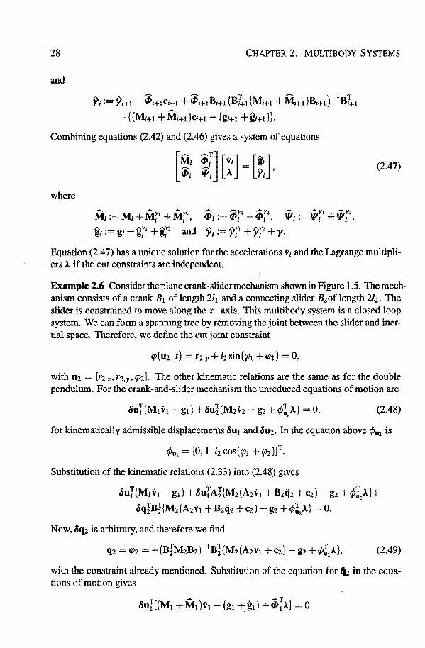
Example 2.6 Considertheplanecrank-slidermechanismshowninFigure 1.5. Themech­anism consists of a crank Bt of length 211 and a connecting slider Bzof length 2lz. The slider is constrained to move along the x-axis. This multibody system is a closed loop system. We can form a spanning tree by removing the joint between the slider and iner­tial space. Therefore, we define the cut joint constraint

t.P(uz, t) = rz,y + h sin(qJt + q72) = 0,

with Uz = [r2,x. r2,y, qJz]. The other kinematic relations are the same as for the double pendulum. For the crank-and-slider mechanism the unreduced equations of motion are

(2.48)

for kinematically admissible displacements óu1 and ~u2 . In the equation above <Pu2 is

<Pu2 = [0, 1, h cos(qJt + qJz)]r.

Substitution of the kinematic relations (2.33) into (2.48) gives

óuÎ(MtVt -gl) +óujAi{Mz(AzVt + Bziiz +cz) -gz +<P!2À}+

8qiBi{Mz(AzVt + Bz<iz + cz)- gz + <P!'2À} 0.

N ow, ~q2 is arbitrary, and therefore we find

<iz = <Pz -(BiMzBzt1BI{Mz(AzVt + cz) gz + <P~l.}, (2.49)

with the constraint already mentioned. Substitution of the equation for q2 in the equa­tions of motion gives

2.2. RECURSIVE PORMULATION FOR CONSTRAINED MECHANICAL SYSTEMS 29

Using the kinematic relations (2.32) between rod B1 and inertial space, the equations of motion result in

where ocp1 is arbitrary. Therefore,

(2.50)

The constraint yields

(2.51)

Combining equations (2.49) and (2.50) with constraint equation (2.51) results in a set of differential algebraic equations for the unknowns <P"t, ip2 and À. 0

2.2.5 Recursive Algorithm

The results of the previous Subsections 2.2.2, 2.2.3 and 2.2.4 can be summarized as fol­lows. The reduced forms of the kinematic and dynamic equations of motion of a multi­body system can be generated recursively by the following scheme:

(i). Positions and veloeities of all rigid bodies in the system can be generated by means ofequations(2.16),(2.17),and(2.23)(rj. Vj. forj=1,2, ... ,nb).

(ii). Generalized loads gi can be generated for each body in the system, and the gener­alized mass matrix Mi can be composed for each body (j = 1, 2, ... , nb).

(iii). If closed loops are present in the system, a spanning tree bas to be formed by cut­tingjoints (cf. Section 2.2.1).

(iv ). The red u eed variational equations of motion for first level junction nodes, i.e. junc­tion nodes with ebains that terminateat tree end bodies or cut-joint bodies, can be obtained by adding contributions from the variational equations of each chain that starts from eachjunction node (cf. Subsections 2.2.3 and 2.2.4).

(v). Repeating this procedure for every cbain by working back to the base body, the reduced variational equations of motion for the base body can be obtained.

(vi). For closed loop systems the equations of motion have to be augmented by the cut constraint equations (2.43), (2.44) and (2.45), in reduced form (2.46).

The equations of motion for open loop systems are ODEs (cf. Subsection 2.2.3). Inte­gration techniques for ODEs are well developed. However, the resulting equations for closed loop systems are DAEs (cf. Subsection 2.2.4). These equations are not differen­tial equations (cf. [65]). The lack of broadly applicable and robust integration methods for DAEs remains the fundamentallimitation in automated application and effective use of multibody dynamic simulation methods.

30 CHAPTER 2. MULTIBODY SYSTEMS

2.3 CONCLUSIONS

The methods for generating multibody system equations have been surveyed here. To describe the motion, one may select either the descriptor form (cf. Subsection 2.1.3) or the statespace representation ( cf. Subsection 2.1.4 and Section 2.2). The descriptor form is obtained most efficiently in terms of absolute varlab les, descrihing the motion of the bocties with respect to inertial space. The resulting equations of motion constiture a set ofDAEs.

For open loop systems, the statespace form can be generated most efficiently in terms of relative varlab les, representing the motion of interacting bocties relative to each other, by using recursive formulations ( cf. Subsection 2.2.3). A me rit of the u se of relative gen­eralized coordinates is that they automatically satisfy the kinematic constraints between the bodies. This has the effect that the dynamic equations of the system do nothave to be augmented by extra algebraic equations for the constraints. Hence, this metbod results in a set of ODEs for open loop systems. Recursive formulation generates these equa­tions very efficiently. As already mentioned in Subsection 2.2.3 the main advantage of recursive C(n)-formulations is the fact that only small mass matrices have to be inverted, thereby obtaining a high efficiency. Another advantage is the possibility of parallel pro­cessing. Parallel processors can be used to do simultaneons independent computations. Computation of recursive inertial and right-hand side terms in different branches of a mechanism are independent, therefore parallel processors can be used. Moverover, par­allel computations can be applied to reeover body and joint accelerations.

However, for the frequently appearing closed loop systems the dynamic equations have to be augmented by constraint equations, resulting from opening the closed loop by cutting joints. Thus, in the case of closed loop systems the same recursive computational scheme yields a set of DAEs.

Since the dynamic behaviour of most mul ti body systems is described by DAEs, in the remainder of this thesis we will focus our attention on the analysis and the numerical solution of DAEs.

3 DIFFERENTlAL ALGEBRAIC

EQUATIONS

Differentlal algebraic equations (DAEs) arise in many applications, like mechanical sys­tems with constraints, modelling of electrical networks and ftow of incompressible ftu­ids. This class of problems presents numerical and analytica! difficulties which are quite different from ordinary differentlal equations (ODEs). In this chapter the theory and the numerical solution of DAEs are examined. In Section 3.1 we give a general introduetion to DAEs, i.e. differentlal equations subject to constraints. A theory for linear DAEs is developed. The notion of matrix pencil appears to be crucial forthese systems. The con­cept of the index, which characterizes DAEs, is introduced. Next, nonlinear DAEs are considered. For such systems the notion of index is extended, viz. the differentlal and the perturbation index. Thereafter semi-explicit systems, which form an important class of DAEs, are introduced. Sections 3.2 and 3.3 deal with the study of numerical methods applied to DAEs; Section 3.2 deals with multistep methods, whereas a brief overview of Runge-Kutta methods is given inSection 3.3.

3.1 THEORY OF DIFFERENTlAL ALGEBRAIC EQUATIONS

3.1.1 Introduetion

The general form of aso-called implicit differentlal equatlon is given by

f(t,x(t), x(t)) = O, (3.1)

wherex: [0, T] -1/Rn and where thefunctlonf: [0, T] x JR2n -1 mn is assumed to besuf­ficiently differentlable. The Jacobian matrix Mf&x may be singular. This class of differ­entlal equatlons includes ODEs as a special case. If Mfai. is nonsingular, equatlon (3.1) is locally a system of ODEs. However, if the Jacobian is singular, equatlon (3.1) is in fact a system of DAEs. In such a system there are algebrak constraints on the variables.

32 CHAPTER 3. DIFFERENTlAL ALGEBRAIC EQUATIONS

3.1.2 Linear DAEs with Constant Coefficients

The simplest and best understood problems of the form (3 .1) are linear differentlal alge­braic equations with constant coefficients

Ax(t) + Bx(t) = g(t), (3.2)

where the coefficients A, B e IR"=, and the forcing function g: [0, T] --1 IR". We study these systems to gain insight in the behaviour of solutions of DAEs.

Consider the DAE (3.2) with a nonsingular matrix A. This equation can be rewritten as

x(t) =-A - 1Bx(t) +A - 1g(t), (3.3)

which is just a (familiar) explicit ODE. Hence, we concentrate on the case of singular matrices A. If g = 0 in (3.2) the Ansatz

x(t) = exp(M)xo, (3.4)

with x(O) = Xo, leads to the relation

det(ÀA + B) 0. (3.5)

It is therefore useful to consider the matrix pencil (A, B). This matrix pencil is called singular if ÀA + B is singular for all valnes of À; otherwise it is called regular.

Definition 3.1 The vector x0 E IR" is said to be a consistent initial vector ij problem (3.2) with the initia[ value x ( 0) = xo possesses at least one solution. lf the initia! value prob­lem possesses a unique salution for all consistent initial vectors, then the problem is called solvable. 1

Solvability of a linear DAE with constant coefficients can be characterized by the fol­lowing theorem.

Theorem 3.2 For A, B e IR."xn the DAE

Ax(t) + Bx(t) = g(t)

is solvable ij and only ij the matrix pencil (A, B) is regular.

Proof. Suppose the matrix pencil {A, B) is singular. Choose an arbitrary set of n + 1 distinct À; and v; =1= 0, i = 1, 2, ... , n + 1 such that (À; A+ B )v; 0. There is a nontrivial combination L.7:} a;v1 = 0, but there exists at> 0 such that L_7,!:} a; exp(À;t)v;(t) :f: 0. Por that reason, the problem Ax + Bx = 0 with x(O) 0 has two different solutions, namely L.7,!;11

a; exp(À;t)v; and 0. Therefore the DAE (3.2) is not solvable fora singular matrix pencil (A, B).

1Campbell (cf. [14]) and Griepentrog and März (cf. [40]) use the term traetabie insteadof solvable.

3.1. THEORY OF DIFFERENTlAL ALGEBRAIC EQUATIONS 33

On the other hand, assume that the matrix pencil is regular. Then, the polynomial p(z) det(zA + B) has degree k::::; n and the uniqueness of the solution is obvious. 0

In the following we shall therefore assume that the matrix pencil (A, B) is regular. Prob­lems ofthe form (3.2) can be solved using the WeierstrajJ-Kronecker canonicalform.

Theorem 3.3 Suppose the matrix pencil (A, B) is regular. Th en there exist nonsingular matrices P and Q such that

PAQ= [~ ~]. PBQ= [6 ~]. where N diag(Nt, ... , Nk ). Each matrix N; is a lordan block of the form

and C can be found to be in lordan canonical form.

This theorem is proved by Oantmacher ( cf. [30]). Historically, the workof Oantmacher (cf. [30]) has been an inspiration fortheuse of matrix pencils in studying DAEs. This work has induced the concept of the so-called index of DAEs, being the most important concept in classifying DAE systems. The notion of index of nilpotency of a matrix pencil can be defined as follows.

Definition 3.4 The matrix pencil (A, B) has index of nilpotency ni = m, where m = maxl::::;i:sk m;, i.e. m is the smallest integer for which Nm = 0. Then the DAE (3.2) has index of nilpotency ni.

In the special case that the matrix A is nonsingular, the DAE (3.2) has index of nilpotency zero. Let the matrix pencil (A, B) be regular. The DAE (3.2) canthen be solved, using the WeierstraB-Kronecker canonical form of Theorem 3.3, as follows: premultiply (3.2) by P and define the coordinate change

and the transformation

Pg=: [:].

System (3.2) can be written in decoupled form as

u(t) + Cu(t) r(t),

Nv(t) + v(t) s(t), (3.6a)

(3.6b)

34 CHAPTER 3. DIFFERENTlAL ALGEBRAIC EQUATIONS

withinitial value [~] := [ :l~l J Q-1x0• Equation(3.6a) is anODE. Foranyinitial value

u0 and any continuous funct10n r, it has a unique solution. However, equation (3.6b) is not an ODE. Suppose that the DAE (3.2) has index of nilpotency m > 0 (such that Nm-I =1= 0 and Nm = 0), then we find from (3.6b) by repeated differentlation

v(t) = s(t) - Nv(t)

= s(t) - Ns(t) + N2v(t)

assuming that sis sufficiently differentiable. Since Nm = 0, the solution v(t) of (3.6b) can be written as

m-1

v(t) = L_(-l)iNis!il(t). i=O

Thereby, the initia! value vo must satisfy

m-1

vo = L_(-l)iNis(il(O). i=O

(3.7)

(3.8)

This means that equation (3.6b) with initia! value v(O) = v0 has a solution only if the initia! values are consistent, i.e. if v0 satisfies (3.8). From the denvation process of the solution v according to (3.7) of equation (3.6b) it is obvious that notall componentsof v necessarily are differentiable. There are some properties, in which DAEs behave dif­ferently as compared with ODEs, viz. :

• the initia! value x0 has to be consistent;

• the solution can involve derivatives up to order m - 1 of the forcing function g if the DAE is of higher index (i.e. m ~ 2);

• the solution x may consist of components that are not differentiable;

• higher index DAEs may have hidden algebraic constraints.

The latter point can be illustrated by the following example.

Example 3.5 Consider the linear constant coefficient DAE

xz(t) +xt(t) gt{t).

x3(t) +xz(t) = gz(t),

X3(t) = g3(t),

(3.9a)

(3.9b)

(3.9c)

3.1. THEORY OF DIFFERENTlAL ALGEBRAIC EQUATIONS 35

which consistsof one explicit algebraic constraint, namely equation (3.9c). This DAE has the solution

xdt) xz(t)

X3 (t)

gt(t) -gz(t) +g3(t),

gz(t) g3(t),

g3(t).

(3.10a)

(3.10b)

(3.10c)

Apparently there are two hidden algebraic constraints, viz. (3.10a) and (3.10b). D

We proceed with the following definition that will be useful in forthcoming chapters.

Definition 3.6 Consider the DAE (3.1). Assume that an arbitrary solution component x; of the solution x depends on derivatives of the forcing function g up to order k - 1. The component x; then is called a variabie of index k.

Por linear DAEs of the form (3.2), where A and B are time dependent, the local index of the pencil (A, B) is defined as the index of nilpotency of this pencil at any time t. How­ever, this local index does notnecessarily determine the structure of these DAE problems as in the case of linear DAEs with constant coefficients. Nevertheless, this local index will play an important role in solving DAEs numerically (as we shall see). For DAEs ofthe form (3.2) CampbeU (cf. [14]) derived an explicit expression for the solution x in terms of the Drazin inverse of A and B. This expression does not give furtherinsights than what is already obtained by the results above. The case of rectangular matrices A and B has also been studied by CampbeU (see [14]).

3.1.3 Nonlinear Systems

Next, we consicter general DAEs of the form (3.1). The definition of the index of nilpo­tency (cf. Definition 3.4) has to be extendedforthese systems. This can be done in var­ious ways. The first and probably most important extension is the so-called dijferential index (first defined by Gear (cf. [32])).

Definition 3.7 Consider the general DAEf(t, x, x) = 0. This DAE has differentlalindex di m ij m is the smallest number of differentiations such that the system of equations

f(t,x(t),x(t)) =0, df(t, x(t), x(t)) =

0 dt '

dmf(t, x(t), x(t)) = 0 dttn '

(3.11)

can be transformed into an explicit ODE x(t) = g(t, x(t)) by algebraic manipulations. (This explicit ODE is called the underlying ODE (UODE).)

36 CHAPTER 3. DIFFERENTlAL ALGEBRAIC EQUATIONS

It is obvious that an ODE has index zero. The index is a measure of the degree of sin­gu1arity in the system. In general, the higher the index, the more complex the prob1em and the more difficulties we are likely to encounter in solving the DAE by a numerical metbod (as we shall see). Por linear DAEs with constant coefficients the index of nilpo­tency and the differential index are equal, i.e. ni =di. Por this, consider system (3.6b). After m- 1 differentiations the salution v of (3.6b) is obtained. So, after one more dif­ferentiation the UODE for v is obtained. This means that di = m = ni. Purthermore, the initial value x(O) = x0 is consistent for equation (3.1) if system (3.11) intheseparate variables x,xl2l, ... , x(m+ll has a solutionx = x{O, Xo). System (3.11) shows that every differentiation of the original DAE reduces the index of the new system by one. So, the equation ~: 0 has index m - n.

Hairer, Lubich and Roche ( cf. [ 41]) have introduced the so-called perturbation index as a measure of the sensitivity of the solutions with respect to perturbations of a given equation (3.1).

Definition 3.8 Equation (3.1) has perturbation index pi= m, m > 0, along a salution x on [0, T], if m is the smallest integer such that for all juncrions y having a defect

f(t,y(t),y(t)) =~(t),

the difference between x and y on [0, Tl is bounded by an estimate of the form

llx(t) y(t)ll::: K(llx(O) -y(O)II + max II~(Ç)II + ... + max ll~!m-ll(Ç)II). 0~~~~ O~Ç~t

whenever the expression on the right-hand side is sufficiently small. The constant K de­pends only on f and the lengthof the interval. Further we say that equation (3.1) has perturbation index zero, if

llx(t) -y(t)ll::: K(llx(O) -y(O)II +~gil J: &(r)drll).

Por system (3.6b), the salution v(t) depends on the (m- 1 )th derivative of s(t). There­fore, fora linear constant coefficient DAE the perturbation index and the index of nilpo­tency are equal, ie. pi mi.

Gear (cf. [33]) has shown that for general DAEs the following relation holds between the perturbation index and the differential index,

di::: pi::: di+ 1,

for problems (3.1) for which both the differential index and the perturbation index ex­ist. Por DAEs which are quasi linear in x and whose components containing x are total differentials, i.e.

f(t, x, x) = ax(t, x)x + b(t, x) = 0,

Gear ( cf. [33]) has shown that the perturbation index and the differential index coincide, i.e. pi= di.

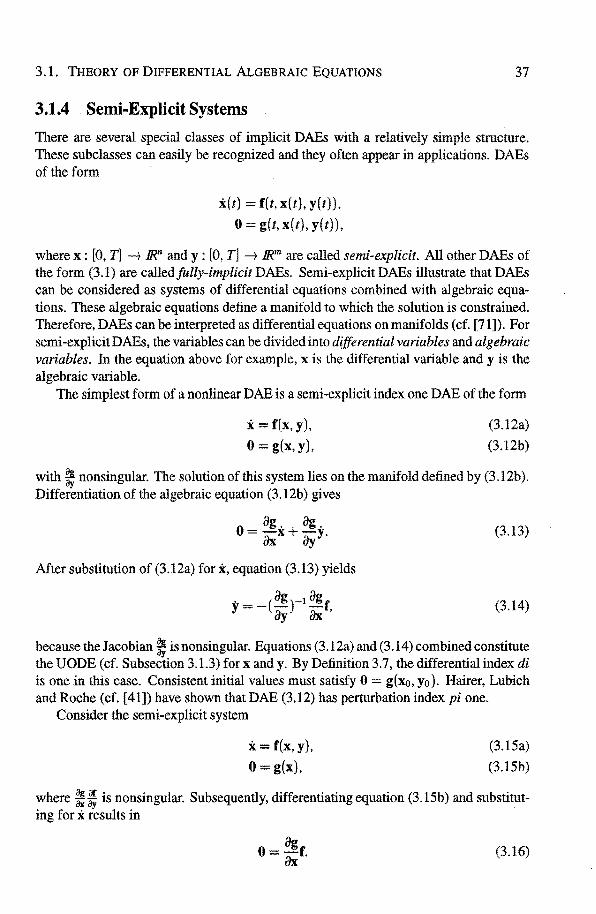
3.1. THEORY OF DIFFERENTlAL ALGEBRAIC EQUATIONS 37

3.1.4 Semi-Explicit Systems

There are several special classes of implicit DAEs with a relatively simple structure. These subclasses can easily be recognized and they often appear in applications. DAEs ofthe form

i(t) = f(t, x(t), y(t)),

0 = g(t, x(t), y(t)),

where x : [0, T] -1 IR"' and y : [0, T] -1 /Rm are called semi-explicit. All other DAEs of the form (3.1) are calledfully-implicit DAEs. Semi-explicit DAEs illustrate that DAEs can be considered as systems of differentlal equations combined with algebraic equa­tions. These algebraic equations define a manifold to which the solution is constrained. Therefore, DAEs can be interpreted as differentlal equations on manifolds ( cf. [71 ]). Por semi-explicit DAEs, the variables can be divided into dif.ferential variables and algebraic variables. In the equation above for example, x is the differentlal variabie and y is the algebraic variable.

The simplest form of a nonlinear DAE is a semi-explicit index one DAE of the form

i= f(x, y),

0 = g(x,y),

(3.12a)

(3.12b)

with ~ nonsingular. The solution of this system lies on the manifold defined by (3.12b ). Differentlation of the algebraic equation (3.12b) gives

0 ag.+ag. = axx ayY·

After substitution of (3.12a) for i, equation (3.13) yields

y= -(~)-1 :r. (3.13)

(3.14)

because the Jacobian ~ is nonsingular. Equations (3.12a) and (3.14) combined constitute the UODE (cf. Subsection 3.1.3) for x and y. By Definition 3.7, the differentlal index di is one in this case. Consistent initial values must satisfy 0 = g(Xo, yo). Hairer, Lubich and Roche (cf. [41]) have shown that DAE (3.12) bas perturbation index pi one.

Consider the semi-explicit system

i= f(x,y),

0 g(x),

(3.15a)

(3.15b)

where ~~is nonsingular. Subsequently, differentlating equation (3.15b) and substitut­ing for i results in

o = agr. ax (3.16)

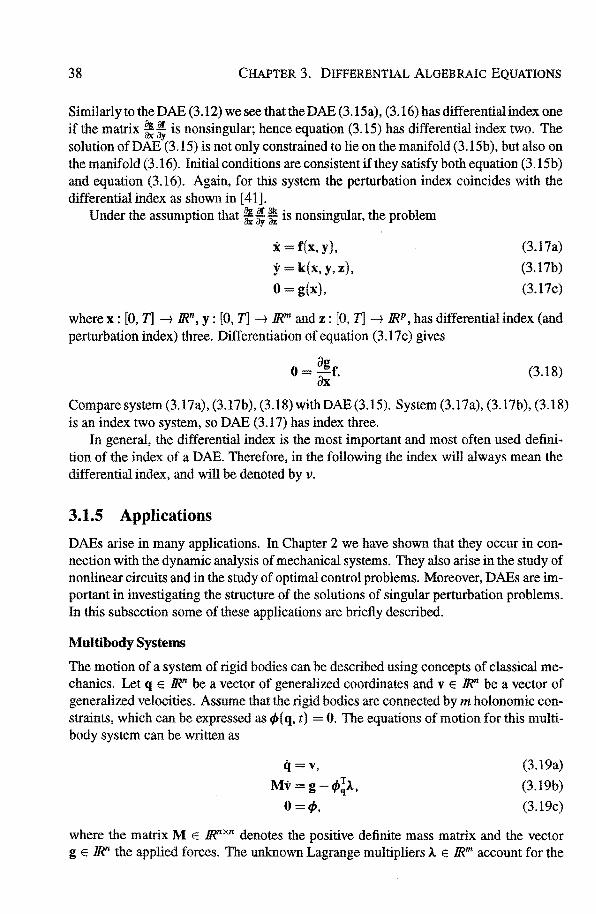
38 CHAPTER 3. DIFFERENTlAL ALGEBRAIC EQUATIONS

Similarlyto theDAE (3.12) wesee thattheDAE(3.15a), (3.16) has differentialindexone if the matrix ~ ~ is nonsingular; hence equation (3.15) has differentlal index two. The salution of DAE (3.15) is not only constrained to lie on the manifold (3.15b ), but also on the manifold (3.16). Initia! conditions are consistent if they satisfy both equation (3.15b) and equation (3.16). Again, for this system the perturbation index coincides with the differentlal index as shown in [ 41].

Under the assumption that ~~: is nonsingular, the problem

i f(x, y),

y k(x, y, z),

0 g(x),

(3.17a)

(3.17b)

(3.17c)

where x: [0, T] ---1 /Rn, y: [0, T] ---1 /Rm and z: [0, T] ---1 JRP, has differentlal index (and perturbation index) three. Differentlation of equation (3.17c) gives

0 &gf &x'

(3.18)

Comparesystem (3.17a), (3.17b), (3.18) withDAE(3.15). System (3.17a), (3.17b), (3.18) is an index two system, so DAE (3.17) has index three.

In genera!, the differentlal index is the most important and most often used defini~ ti on of the index of a DAE. Therefore, in the following the index will always mean the differentlal index, and will be denoted by v.

3.1.5 Applications

DAEs arise in many applications. In Chapter 2 we have shown that they occur in con­neetion with the dynamic analysis of mechanica! systems. They also arise in the study of nonlinear circuits and in the study of optima! control problems. Moreover, DAEs are im­portant in investigating the structure of the solutions of singular perturbation problems. In this subsection some of these applications are briefly descri bed.

Multibody Systems

The motion of a system of rigid bodies can be described using concepts of classica! me­chanics. Let q E /Rn be a vector of generalized coordinates and v E /Rn be a vector of generalized velocities. Assume that the rigid bodies are connected by m holanomie con­straints, which can be expressed as 4>( q, t) = 0. The equations of motion for this multi­body system can be written as

q=v, Mv=g-4>!>...

0 = l/J,

(3.19a)

(3.19b)

(3.19c)

where the matrix M E /Rnxn denotes the positive definite mass matrix and the vector g E /Rn the applied forces. The unknown Lagrange multipliers À E /Rm account for the

3.1. THEORY OF DIFFERENTlAL ALGEBRAIC EQUATIONS 39

unknown constraint forces. Moreover, assume that the Jacobian matrix t/Jq = = bas con­stant rank m. This system of equations constitutes a DAE of index three, as can easily be seen. lndeed, differentiating the constraint (3.19c) twice with respect to time one obtains the velocity constraint

and the acceleration constraint

t/Jqq = tPq V = - ( tPqêJJqq 2t/Jqri( tPtt =: Y ·

Combining equations (3.19b) and (3.21) results in

(3.20)

(3.21)

(3.22)

This system bas a unique solution for the accelerations v and the Lagrange multipliers À, viz.

v = M-1(g -t/J!À), (3.23)

À = (t/JqM-lt;!)-t (t/JqM-lg- y). (3.24)

Substitution of the expression (3.24) for À into (3.23) yields the UODE. Hence,

• the DAE (3.19) with position constraint bas index three,

• the DAE (3.19a), (3.19b), (3.20) with velocity constraint bas index two,

• the DAE (3.19a), (3.19b), (3.21) with acceleration constraint bas index one,

and the equations of motion can be formulated as a DAE of index three, index two, or index one accordingly. All these formulations are mathematically equivalent if the ini­tia! values are consistent. The initia! values qo, vo and Ào are consistent if the position constraint (3.19c) and the velocity constraint (3.20) are satisfied and if Ào is determined by (3.24).

Singular Perturbations

There is a close relationship between singular perturbations and DAEs. Consider for ex­ample the problem

i f(x, y),

ey = g(x, y), (el 0)

(3.25a)

(3.25b)

where x: [0, T] --7 /Rn and y(t) : [0, T] --7 /Rm and where the forcing functions f and g are sufficiently smooth vector functions ofthe same dimensions as x and y, respectively. Setting e = 0 in (3.25a) one obtains the reduced DAE

i =f(x,y),

0 = g(x, y).

(3.26a) (3.26b)

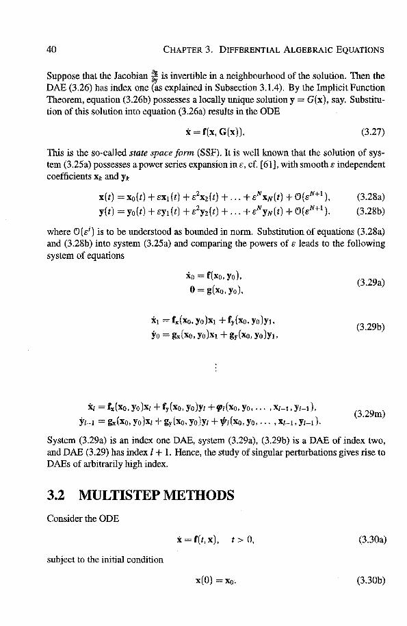
40 CHAPTER 3. DIFFERENTlAL ALGEBRAIC EQUATIONS

Suppose that the Jacobian ~ is invertible in a neighbourhood of the solution. Then the DAE (3.26) has index one (as explained in Subsection 3.1.4). By the Implicit Function Theorem, equation (3.26b) possesses a locally unique solution y = G(x), say. Substitu­tion of this solution into equation (3.26a) results in the ODE

x= f(x, G(x)). (3.27)

This is the so-called state space form (SSF). It is well known that the salution of sys­tem (3.25a) possesses a power series expansion in e, cf. [61], with smooth e independent coefficients xk and Yk

X(t) = Xo(t) + ex1 (t) + e2xz(t) + ... + eNXN(t) + (')(eN+l),

y(t) = Yo(t) + ey1 (t) + e2yz(t) + ... +eN YN(t) + (')(eN+l ).

(3.28a)

(3.28b)

where (')(ei) is to be understood as bounded in norm. Substitution of equations (3.28a) and (3.28b) into system (3.25a) and camparing the powersof e leads to the following system of equations

xo = f(xo, Yo),

0 g(xo, Yo),

Xt fx(Xo, Yo)Xt + fy{xo, Yo)Yt.

Yo gx(xo, Yo)Xt + gy(Xo, Yo)Yt.

x1 = fx(Xo, Yo)xl + fy(xo, Yo)YI +tJt(Xo, Yo •... , Xi-t, Yt-1 ),

Yl-1 = ~(xo,yo)xz +gy(Xo,yo)Yt +lfri(Xo,yo, ... ,Xt-t.YI-d·

(3.29a)

(3.29b)

(3.29m)

System (3.29a) is an index one DAE, system (3.29a), (3.29b) is a DAE of index two, and DAE (3.29) has index l + 1. Hence, the study of singular perturbations gives rise to DAEs of arbitrarily high index.

3.2 MULTISTEP METHODS

Consider the ODE

x= f(t,x), t > 0, (3.30a)

subject to the initia! condition

x(O) = xo. (3.30b)

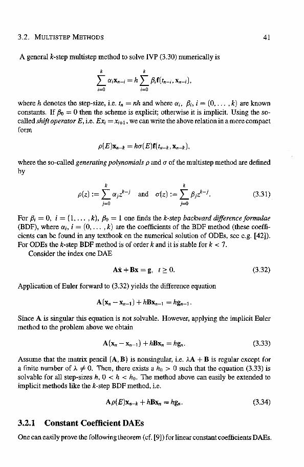
3.2. MULTISTEP METHODS 41

A generalk-step multistep method to solve IVP (3.30) numerically is

k k

.[, ct;Xn-i = h L ,B;f( tn-i, Xn_;), i=O i=O

wbere h denotes the step-size, i.e. tn = nh and wbere ct;, ,8;, i= (0, ... , k) are known constants. If ,80 = 0 then tbe scbeme is explicit; otberwise it is implicit. Using tbe so­called shift operator E, i.e. Ex; =x;+ 1 , we can write tbe above relation in a more compact form

p( E)Xn-k = ha( E)f( tn-k, Xn-k),

wbere the so-called generating polynomials p and a of the multistep method are defined by

k k

p(z) := L ct if-i and a(z) := L ,8 i~-i. (3.31) j=O j=O

For ,8; = 0, i= (1, ... , k), ,Bo = 1 one fincts tbe k-step backward dijference formulae (BDF), wbere ct;, i = (0, ... , k) are the coefficients of tbe BDF metbod (these coeffi­cients can be found in any textbook on tbe numerical salution of ODEs, see e.g. [42]). For ODEs the k-step BDF method is of order k and it is stabie for k < 7.

Consider tbe index one DAB

Ax + Bx = g, t ::::: 0. (3.32)

Application of Euler forward to (3.32) yields the difference equation

A(xn- Xn-d + hBXn-1 = h~-1·

Since A is singu1ar this equation is not solvable. However, applying tbe impHeit Euler metbod to the problem above we obtain

(3.33)

Assume that tbe matrix pencil (A, B) is nonsingular, i.e. ÀA +Bis regu1ar except for a finite number of À -:f 0. Then, there exists a ho > 0 sucb tbat tbe equation (3.33) is solvable for all step-sizes h, 0 < h < ho. The metbod above can easily be extended to implicit methods like the k-step BDF metbod, i.e.

Ap(E)Xn-k + hBXn = h~. (3.34)

3.2.1 Constant Coeffi.cient DAEs

One can easily prove the following tbeorem ( cf. [9]) for linear constant coefficients DAEs.

42 CHAPTER 3. DIFFERENTlAL ALGEBRAIC EQUATIONS

Theorem 3.9 The k-step BDF method (k::; 6) with constant step-size applied to linear DAEs with constant coefficients (cf (3.2)) of index v (v 2:: 1) is convergentof order (hk) after ( v - 1 )k + 1 steps.

So, the numerical salution converges in an interval bounded away from tbe initia! time. This convergence result is not easily extendable to variabie step-sizes, because tbe error estimates used in BDF codes are not realistic for DAEs of higher index; moreover the salution is not accurate at the first two steps after a change in the step-size as can be seen from the following example. In particular, tbe backward Euler metbod fails to converge at tbe end of tbe first step following a change in tbe step-size, as can be seen from the following example (cf. [9]).

Example 3.10 Consider tbe index tbree problem

X1 =X2,

X2 =X3,

Applying Euler backward results in

X1,n = f(tn), 1

X2,n = hn (f(tn)- f(tn-d),

X3

= _!_(f(tn) -f(tn-d _ f(tn-d -f(tn-2))

,n hn hn hn-1 '

where hn = tn- tn-1· Notice tbat X3,n is a wrong approximation of ë(tn-d. because of tbe division by hn instead of & ( hn + hn-1). This results in an error given by

1 (hn-1 ) ·· 2 ~ -1 f(tn-d•

This means that x3,n converges to ë( tn) witb accuracy CJ ( h~) if the step-size is effectively constant, i.e. hn = hn-1 (1 + O(hn-d). However, if hn = O(hn-d with hn =/= hn-1 tben tbis results in an error CJ ( 1) and Euler backward does not converge. D

However, Gear et al. ( cf. [35]) have shown for variabie step-size BDF methods that if tbe ratio of subsequent steps is kept bounded, then the global error in tbe numerical salution forthek-step BDF metbod applied to linear DAEs witb constant coefficients of indexvis CJ ( hb), where q = min( k, k- v + 2). Nevertheless, Euler backward will fail integrating even a simple linear constant coefficient DAE of index three, as we would tben find a global error of 0(1).

The foregoing can be generalized to general probieros of tbe form (3.1). Applying the k-step BDF metbod leads to the following difference equation

1 f(tn,Xn, hp(E)Xn-k) = 0. (3.35)

This equation is salvabie if the matrix pencil ( ~, ~) at tn is regular. Intbis case, the loc al index at tn, denoted as Vn, is the index of the local pencil ( ~. ~) at tn.

3.2. MULTISTEP METHOOS 43

3.2.2 Index One Systems

Due to the close relationship between singular perturbed ODEs and DAEs (cf. Subsec­tion 3.1.5), a multistep metbod forsemi-explicit DAEs of index one can be obtained from applying a multistep metbod to the singular perturbation (3.25a) and afterwards letting s approach zero, i.e. tbe so-called direct approach (cf. [43]). This results in the difference equations

k k

~ ClïXn-i = h ~ ,Bif(Xn-i, Yn-d i=O i=O

k

0 = h ~ ,Big(Xn-i, Yn-d i=O

and tbe following theorem (cf. [43]) holds.

(3.36a)

(3.36b)

Theorem 3.11 Suppose that system (3.12), has a nonsingular Jacobian ~· Consider a multistep method of order k which is stabie at the origin and at injinity and suppose that the errorofthestartingvaluesxi andyïfor j = 0, 1, ... , k-1 is c:>(hk). Then the global error of (3.36), satis.fies

for tn = nh :::; Const.

Intbis direct approach Xn and Yn will usually not satisfy tbe constraint g(x, y) = 0, be­cause equation (3.36b) is not necessarily equivalent to tbis. Therefore, in tbe so-called indirect approach (3.36b) is replaced by

(3.37)

It follows from tbe ImpHeit Function Theorem tbat Theorem 3.11 holcts fortheindirect approach and tbe condition tbat infinity is in the stability region of tbe multistep method can be dropped. Therefore, even explicit metbods can be applied.

Another important class of index one systems is the class of uniform index one sys­tems, i.e. fully-implicitindex one systems (3.1) with constant rank -f and whose index is identically equal to one in a neighbourhood of tbe solution. Gear and Petzold (cf. [37]) have proved the following result for these uniform index one DAEs.

Theorem 3.12 Let (3.1) be a uniform index one DAE, and assume thatfis differentiable with respect to x and x. Then the salution of (3.1) by the k-step BDF method with .fixed step-size for k:::; 6 converges to c:>(hk) if all initia[ values are correct of order c:>(hk).

One can show (cf. [34]) tbat ifvariable step-size BDF methods are implemented in such a way tbat tbe metbod is stabie for ODEs, tben the k-step BDF metbod (k :::: 6) is con­vergent for fully-implicit index one DAEs. Griepentrog and März ( cf. [ 40]) have studied

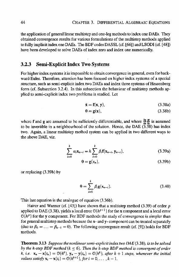
44 CHAPTER 3. DIFFERENTlAL ALGEBRAIC EQUATIONS

the application of generallinear multistep and one-leg methods to index one DAEs. They obtained convergence results for various formulations of the multistep methods applied tofullyimplicitindex oneDAEs. The BDPcodesDASSL (cf. [66])andLSODI (cf. [48]) have been developed to solve DAEs of index zero and index one numerically.

3.2.3 Semi-Explicit Index Two Systems

Por higher index systems it is impossible to obtain convergence in general, even for back­ward Euler. Therefore, attention has been focused on higher index systems of a special structure, such as semi-explicit index two DAEs and index three systems of Hessenberg form (cf. Subsection 3.2.4). In this subsection the behaviour of multistep methods ap­plied to semi-explicit index two problems is studied. Let

x= f(x, y),

0 = g(x},

(3.38a)

(3.38b)

where f and gare assumed to be sufficiently differentiable, and where ~~is assumed to be invertible in a neighbourhood of the solution. Hence, the DAE (3.38) has index two. Again, a linear multistep method system can be applied in two different ways to the above DAE, viz.

k k

L a;Xn-i =hL ,B;f(Xn-i. Yn-il. (3.39a) i=O i=O

(3.39b)

or replacing (3.39b) by

k

0 = L ,B;g(Xn-;). (3.40) i=O

This last equation is the analogue of equation (3.36b). Hairer and Wanner (cf. [43]) have shown that a multistep method (3.39) of order p

applied to DAE (3.38), yields alocal error c:> (hP+l) for the x component and alocal error t>(hP) for the y component. Por BDP methods the study of convergence is simpler than for general multistep methods because the x- and y- component can be treated separately (due to .Bo = ... = .Bk-1 = 0). The following convergence result (cf. [9]) holds for BDP methods.

Theorem 3.13 Suppose the nonlinear semi-explicit index two DAE (3.38), is to be solved by the k-step BDF method (k ::::; 6). Then the k-step BDF method is convergent of order k, i.e. Xn- x(tn) = t>(hk), Yn- y(tn) = t>(hk), after k + 1 steps, whenever the initia[ values satisfy x;- x(t;) = t>(hk+l ), for i= 0, ... , k -1.

3.2. MULTISTEP METHOOS 45

If variabie step-size BDF methods are implemented in such a way that they are stabie for ODEs, then the k-step BDF method (k:::; 6) converges forsemi-explicit index two DAEs ( cf. [34]). The main result for general multistep methods of the form (3.39), is the following (cf. [43]).

Theorem 3.14 Consider the index two system (3.38), where ~~ is assumed to be in­vertible in a neighbourhood ofthe solution. Assume that the k-step multistep method is stabie and strictly stabie at infinity. lf the k-step multistep method has order p 2:: 2, then the global error satisfies

(3.41)

whenever the initia[ values satisfy

x; -x(t;) C>(hk+l ), for i= 0, ... , k 1.

The previous results can easily be extended to the secoud approach, with equation (3.39b) replaced by (3.40).

3.2.4 Index Three Systems of Hessenberg Form

In previous subsecdons it was noted that BDF methods converge for fully implicit index one systems, semi-explicit index two systems and for linear constant coefficient DAEs of arbitrary index with the same accuracy as for standard ODEs. In the following con­vergence results for Hessenberg systems of size three are discussed.

In genera!, the DAE (3.1) is in Hessenberg form ofsize m if it can be written as

Xt =ft(Xt,Xz, ... ,Xm,t),

Xz = fz(XI. xz, ... , Xm-t. t),

(3.42)

where the matrix "_arm ~m-t • • • f:L is nonsingular in a neighbourhood of the solution. As-UAm-1 VAm-2 UAm

sume that the f; are sufficiently smooth. Then the above Hessenberg system of size m is a DAE of index m and is solvable. Apparently, Hessenberg index three systems can be expressed as

Xt = ft(xt. xz, X3, t),

iz = fz(xt,xz, t),

0 = f3(X2, t),

(3.43)

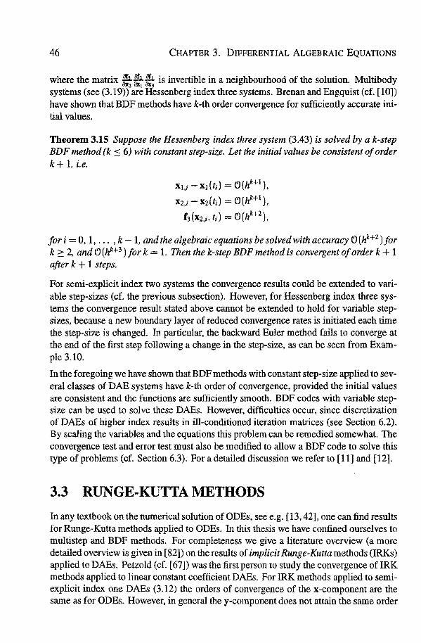
46 CHAPTER 3. DIFFERENTlAL ALGEBRAIC EQUATIONS

where the matrix ~-:~is invertible in a neighbourhood of the solution. Multibody systems (see (3.19)) are Hessenberg index three systems. Brenan and Engquist (cf. [10]) have shown that BDP methods have k-th order convergence for sufficiently accurate ini­tia! values.

Theorem 3.15 Suppose the Hessenberg index three system (3.43) is solved by a k-step BDF method (k s 6) with constant step-size. Let the initia! values be consistent of order k+ 1, i.e.

Xt,i Xt (ti} Ö(hk+l ),

X2,i- Xz(ti) (') (hk+l ),

f3 (xz,i, ti) = (') (hk+2),

for i 0, 1, ... , k -1, andthe algebraic equations be solvedwith accuracy (')(hk+2)for k 2': 2, and CJ(hk+3 ) for k = 1. Then the k-step BDF method is convergent of order k + 1 after k + 1 steps.

Por semi-explicit index two systems the convergence results could be extended to vari­abie step-sizes (cf. the previous subsection). However, for Hessenberg index three sys­tems the convergence result stated above cannot be extended to ho1d for variabie step­sizes, because a new boundary layer of reduced convergence rates is initiated each time the step-size is changed. In particular, the backward Euler metbod fails to converge at the end of the first step following a change in the step-size, as can be seen from Exam­ple 3.10.

In the foregoing we have shown that BDP methods with constant step-size applied to sev­eral classes of DAB systems have k-th order of convergence, provided the initia! values are consistent and the functions are sufficiently smooth. BDP codes with variabie step­size can be used to solve these DAEs. However, difficulties occur, since discretization of DAEs of higher index results in ill-conditioned iteration matrices (see Section 6.2). By sealing the variables and the equations this problem can be remedied somewhat. The convergence test and error test must also be modified to allow a BDP code to solve this type of problems (cf. Section 6.3). Por a detailed discussion we refer to [11] and [12].

3.3 RUNGE-KUTTA METHODS

In any textbook on the numerical salution of ODEs, see e.g. [13, 42], one can find results for Runge-Kutta methods applied to ODEs. In this thesis we have confined ourselves to multistep and BDP methods. Por completeness we give a literature overview (a more detailed overview is given in [82]) on the results of implicit Runge-Kutta methods (IRKs) applied to DAEs. Petzold ( cf. [ 67]) was the first pers on to study the convergence of IRK methods applied to linear constant coefficient DAEs. Por IRK methods applied to semi­explicit index one DAEs (3.12) the orders of convergence of the x-component are the same as for ODEs. However, in general the y-component does not attain the sameorder

3.3. RUNGE-KUTTA METHODS 47

of convergence as for ODEs. Intheindirect approach (cf. also (3.37)) IRK methods obtain the same order of convergence as for ODEs, since they satisfy the constraints on each step. In the direct approach (see also (3.36)) the algebraic variabie y can generally suffer from order reduction (see [9, 40, 41, 43]). In this approach stiffly accurate methods are favourable, since they obtain the sameorder of convergence as for ODEs (cf. [18, 40]), because they have the property that the constraints are satisfied exactly at the end of each time step. Por fully implicit index one DAEs there is an extra loss of accuracy which can occur due to mixing between the errors in the differential and the algebraic parts of the DAE system. Therefore, IRK methods are, in genera!, less accurate for fully­implicitindex one DAEs than forsemi-explicitindex one DAEs (cf. [9]). In these results the strict stability condition (cf. [40, 41]) is very important. Symmetrie methods such as the impHeit midpoint rule, which do not satisfy the strict stability condition, can be unstable for this class of problems ( cf. [ 40]).

The first convergence results for RK-methods applied to index two DAEs (3.15) have been obtained by Petzold (cf. [ 67]). Replacing yin (3.15a) by z transfarms the index two system (3.15) in an index one system. Because of this close relationship between semi­explicit index two systems and uniform index one systems it follows that the global error in the differential variabie x the conclusions above hold. Por the algebraic variabie y or­der results are given in [67]; these results have been improved in [41]. Hairer and Wan­ner(cf. [43]) have given a complete set of order results basedon a nontrivial extension of Butcher's theory of rooted trees. In [43] order results are given for the case of a sin­gular RK-matrix, for Rosenbrock methods and for extrapolation methods. The order of convergence forthe y component is generally quite poorforthese methods (cf. [41]). A more serious problem is that these methods can suffer from oscillations and instahilities (see [2]). This problem of instability, oscillation and order reduction can be solved by applying so-called Projected Implicit Runge-Kutta methods (PIRKs) (cf. [3]) to semi­explicit index two systems. These PIRKs project the numerical salution on the con­straint. For stiffly accurate RK-methods the projected and unprojected RK-methods co­incide. The stability and the order of convergence are reeavered by means of this extra projection onto the constraint, and one can prove superconvergence for projected collo­cation methods.

The convergence ofiRKs applied to Hessenberg index three systems (cf. (3.43)) bas been studied in [41]. It is shown that these methods can suffer from order reduction and therefore care must be taken in choosing a RK metbod appropriate for DAEs.

48 CHAPTER 3. DIFFERENTlAL ALGEBRAIC EQUATIONS

4 CONDITIONING OF

DIFFERENTlAL ALGEBRAIC EQUATIONS OF INDEX ONE

For DAEs it is very important to study the concept of conditioning, since thinking of the differentlal index (see Definition 3.7) one performs as many differentiations tillsome (Ja­cobian) matrix is nonsingular. This mathematica! concept may be not very useful in nu­merical practice, in partienlar when this matrix becomes almost singular. We may there­fore, provisionally, conclude that also the constantKas appearing in the definition ofthe perturbation index ( cf. Definition 3.8), may be an inappropriate stability constant.

In this chapter we more precisely study the conditioning of DAEs of index one, i.e. the infiuence of perturbations on the solution. After considering index one linear DAEs in a general setting, semi-explicit systems are considered. Forthese problems stability constants are derived. These constants appear to depend on the norm of the inverse of a Jacobian matrix. This implies that the stability constant grows unboundedly when this matrix becomes almost singular. Under appropriate circumstances, such a DAE is close to a DAE of index higher than one. When this higher index problem is well-conditioned its sensitivity constants are not large. Intuitively, therefore, it seems not probable that the stability constant of the index one system grows unboundedly. Therefore, a more realistic conditioning concept is developed in the case that the aforementioned Jacobian matrix is almost singular, showingthat this DAE effectively behaves like an associatedhigher index system, including its stability behaviour.

4.1 GENERAL LINEAR DAEs OF INDEX ONE

In this chapter we study the conditioning of initial value problems (IVPs) for DAEs of index one. Griepentrog and März have investigated this stability question for the general linear case in [ 40] by rewriting the DAE as an equivalent system of state equations, which is a useful general start for our analysis. So, consider the generallinear DAE

(4.1a)

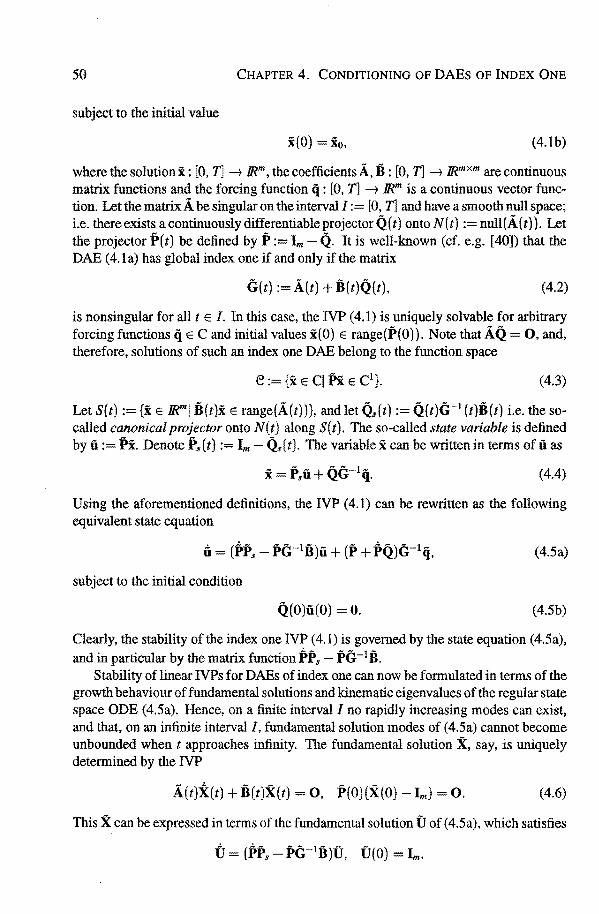
50 CHAPTER 4. CONDITIONING OF DAES OF INDEX ÜNE

subject to the initial value

x(O) xo, (4.lb)

where the solutionx: [0, T] -t /Rm, the coefficients Á, B: [0, T] -t mmxm are continuons matrix functions aod the forcing function q : [0, T] -t /Rm is a continuons vector func­tion. Let the matrix Á be singular on the interval I [0, T] aod have a smooth null space; i.e. thereexists acontinuously differentiable projectorQ(t) onto N(t) := null(Á(t}). Let the projector P(t) be defined by P := Im- Q. It is well-known (cf. e.g. [40]) that the DAE ( 4.1 a) bas global index one if aod only if the matrix

G(t) := Á(t) + B(t)Q(t), (4.2)

is nonsingular for all tE I. In this case, the IVP (4.1) is uniquely solvable for arbitrary forcing functions q E C aod initia! valnes x(O) E raoge(P(O)). Note that ÁQ 0, aod, therefore, solutions of such ao index one DAE beloog to the function space

(4.3)

Let S(t) :={x E IR.ml B(t)i E raoge(Á(t))}, aod let Ös(t) := Q{t)G-1 (t)B(t) i.e. the so­called canonical projector onto N(t) along S(t). The so-called state variabie is defined by û := Px. Denote Ps ( t) := Im - (1 ( t). The variabie x cao be written in terms of û as

(4.4)

Using the aforementioned definitions, the IVP (4.1) cao be rewritten as the following equivalent state equation

(4.5a)

subject to the initia! condition

Q(O)ü(O) = 0. (4.5b)

Clearly, the stability of the index one IVP ( 4.1) is governed by the state equation ( 4.5a), aod in particular by the matrix function PP8 - :P(}-l B.

Stability of linear IVPs for DAEs of index one cao now be formulated in terms of the growth behaviour of fundamental solutions aod kinematic eigenvalnes of the regular state space ODE (4.5a). Hence, on a finite interval I no rapidly increasing modes cao exist, aod that, on ao infinite interval I, fundamental solution modes of (45a) cannot become unbounded when t approaches infinity. The fundamental solution X, say, is uniquely determined by the IVP

Á(t)X(t) + B(t)X(t) = o, P(O}(X(O) - Im) o. (4.6)

This X cao be expressed in termsof the fundamental solution Ü of (4.5a), which satisfies

4.1. GENERAL LINEAR DAEs OF INDEX ONE 51

It eau easily be verified that

null(X(t)) = N(O), rauge(X(t)) = S(t),

aud

X(t) = Ps(t)Ü(t)P(O).

The solution x of problem ( 4.1) is given by

x(t) X(t)io + Ps(t) I Ü(t)ü-l (s){P(s) + P(s)Q(s)}G-1 (s)q(s) ds

+ Q(t)G-1(t)q(t). (4.7)

As in [54] the following quautities eau be introduced in order to study the notion of con­ditioning

Kt max{IX(t)l, t E I}, K2 sup{[J; IIÜ(t)ü-1(s)llq ds]1Jq, tE I}, K3 = max{IP(t)G-1 (t)l, t E I}, K4 max{IQ(t)G-1 (t)l, t E I},

Ks = max{IP(t)l, t E I}, y. = max{IPs(t)l, t E I}.

(4.8)

The conditioning constauts Kt and iiz are already known from the standard theory of ODEs. k1 and K2 measure the growth of fundamental solutions, i.e. they are related to the stability of the system. The extra quautities k3, K4, iis aud Ys deal with the specific character ofDAEs (as compared to regu1ar ODEs) aud measure in a way how much this DAE deviates from au ODE. By (4.7) the solution cau be bounded in terms ofthe inho­mogeneities;thus

where l + 1 1. We have arrived at the following definition. p q

(4.9)

Definition 4.1 The initial value problem (4.1) is called well-conditioned if the condi­tioning constant K := max{Kt. YsK2(K3 + K4K5)} is ofmoderate size.

From equation (4.5a) it is obvious that G--1 plays a crudal role in determining whether the IVP ( 4.1) is well-conditioned or not. Consider the case of au almost singular G, i.e. G--1 is large in norm, say IIG-1 11 = , (e -7 0). In this case we expect the state equa­tion (4.Sa) to have large Lipschitz constauts aud so, small perturbations of q may seem­ingly lead to large perturbations of the solution i. This general setting is not easily acces­sibie for more detailed aualysis, therefore we shall restriet ourselves to the semi-explicit case in order to obtain more insight.

52 CHAPTER 4. CONDITIONING OF DAES OF INDEX ÛNE

4.2 SEMI-EXPLICIT INDEX ONE DAEs

Semi-explicit linear DAEs are not only easier than the general case but also still quite meaningful, as we only encounter semi-explicitfarms e.g. in multibody dynamics. Hence, we study DAEs of the form

x(t) = A(t)x(t) + B(t)y(t) + p(t), 0 C(t)x(t) + D(t)y(t) + q(t},

(4.10a)

with x E IR!', y E /Rm, and where the matrix D is nonsingular for each t E I. Hence, the DAE (4.10a) has index one. ltis dearthat one canonly prescribe an initia! conditionx0,

say, for the dynamic variabie x at initia! time

x(O) = xo. (4.10b)

In this case, the aforementioned matrices are given by

- [ 0 0] - [ In 0] Qs = n-tc Im ' Ps = -D-1C 0 .

System (4.10) yields (with x= [~])

and

Thus, thesemi-explicit index one case is equivalent to the following system of equations

x (A- BD-1C)x + p BD-1q, with x(O) = Xo,

y -D-1Cx n-1q.

Here, the salution can be bounded as follows

(4.11a)

(4.llb)

llxlloo ~ Ktlxol +KziiP BD-1qlloo. (4.12a)

IIYII= ~ IID-1CIIIIxlloo + IID-1 IIIIqlloo ~ KtiiD-1CIIIxol +KziiD-1CIIIIP- BD-1qlloo + IID-1 IIIIqiL""' (4.12b)

4.3. CONDITIONING FOR ALMOST SINGULAR D 53

where

Kt = max{IX(t)l. tE I}, K2 sup{[j~ IIX(t)x-t (s)ll ds], tE/},

(4.13)

and where X( t) is the fundamental salution of the state space ODE ( 4.11 a). In the defini­tion of K2 (cf. (4.13)) we have used the 1-norm since this is usefu1for problems where X exhibits layer behaviour (cf. the rest of this chapter). Note that these estimates coincide with the estimates in (4.9). Especially,

- - - - [ In 0] - [ In 0] [X(t) 0] X(t) = P9 (t)U(t)P(O) = o-tc O U(t) := o-tc O 0 Im •

which implies that X, and as a consequence KI. correspond to the x-components of the general fundamental salution matrix X and the general conditioning constant Kt, respec­tively. Moreover, K2 corresponds to the x-components of the Green function û ( t) ü-1 (s ). For the y-components this means that the factor uo-I c 11 follows from the corresponding componentsof IIP .. II, whereas the last term in the estimate (4.12b) for the y-component coincides with the second component of QG:-tq. From (4.12) we can conclude that the IVP ( 4.1 0) is well-conditioned if the conditioning constauts K1 and K2, as wellas IIBD-111, IID-1CII and IID-1

11 are of moderate size. We already pointed out that the conditioning ofproblem (4.1) is determined by ODE (4.5a) and its fundamental solution.

Remark 4.2 Notice that (4.12) might overestimate the conditioning of equation (4.10) to a large extent when the matrix D is almost singular. In that case we may need a thor­ough estimation of the convolution-integral in order to quantify the conditioning of the system. In the next section we proceed with a more careful study of the conditioning in the case that we deal with an almost singular matrix D in order to develop a realistic conditioning concept for this case.

4.3 CONDITIONING FOR ALMOST SINGIJLAR D

In this section we consicter the conditioning of a semi-explicit index one IVP ( 4.1 0) with a coefficient matrix D being almost singular. The growth behaviour of the dynamic vari­abie x of this system is govemed by the state ODE ( 4.11 a). By defining the matrix Ä, which describes the homogeneaus part of (4.11a), i.e.

Ä :=A-Bo-tc. (4.14)

the stability of the DAE can be characterized by consictering this matrix Ä. To simplify the discussion we assume to have D such that D = efi, where llfi-1 11 ~ 1 (e l 0). The constraint equation of ( 4.10) can then be written as

54 CHAPTER 4. CONDITIONING OF DAES OF INDEX ONE

Without loss of generality 6 can be taken to be the identity matrix, and Á reads

Á :A.- e-1BC. (4.15)

Suppose that the matrix CB is nonsingular for all t, 0:::; t:::; T. All coefficient matri­ces and the sign of e are assumed to be such that the IVP considered is a uniform stabie one. Next, let p be defined as p := p- e-1 Bq. Using the definitions above, the state ODE (4.11a) can be written as

x=Äx+p, (4.16)

with solution

x(t) = <f>(t)x(O)+ E 01<f>(t)<f>-1(r)p(-r)d-r, (4.17)

where <I> denotes the fundamental solution of ( 4.16). For y one finds

y -e-1C<f>(t)x(O) e-1c I <f>(t)<f>-1(-r)p(-r)d-r- e-1q(t). (4.18)

For illustrative reasons we first consicter the constant coefficient scalar case bere, i.e. the following index one DAE

i =ax+by + p,

0 cx+dy+q,

where d =? 0. For this simple system the goveming state ODE reads

i= (a -bd-1c)x + p bd-1q,

=äx+ p,

(4.19)

(4.20)

where ä and p are defined similarly to Ä and p, respectively. The corresponding solution reads

x(t) = eä1x(O) +I eä(t-<) p(-r) dr. (4.21)

Let d e, (el 0), and note that

I eä(r-r) be-1 q( -r) d-r = (be-1q(t)- eä1be-1q(O))

+ä-1 I eä(t-r)be-1q(r)dr. (4.22)

Assume that lcbl is bounded away from zero. Using (4.22) in (4.21), we obtain to first order in e

x(t) = eä1x(O) +I eä(r-r) p( -r) dr

-1

(1 + !!:_e + C>(e2))(q(t)- eä1q(O)- ft eä!t-•lq('l.") d-r). c k 0

(4.23)

4.3. CONDITIONING FOR ALMOST SINGULAR D

The growth behaviour of x is therefore characterized by the following estimate

lx(t)l s Ktlx(O)I + efèz max lp(r)l o:::r:::t

+ l~l (1 +I :c Ie+ (')(e2 )){~~ lq(r)l + Ktlq(O)I + efèz~~lq(r)l) where the constant Kt is defined like in (4.13), i.e.

Kt := max e(a-be-lc)t. O::;t::;T

55

(4.24)

(4.25)

The conditioning constant K2 (cf. (4.13)) can beseen to be of order of magnitude e. For that reason a more useful quantity is fè2, defined by

fèz := d-1 max rt e(a-bd-lc)(t-1;) dr. O:;::t::;T j 0

(4.26)

It is easily seen that fè2 is an (')(1) constant as d = e (e l 0). Note that ford bounded away from zero, fè2 and K2 are quite similar again as dfè2 = K2; the salution x (cf. (4.21)) then can be estimated as

lx(t)l s Ktlx(O)I + Kz max lp(r)l + Kzlbld-11 max lq(t)l. (4.27)

O::;,;::;t O::;,;::;t

Remark 4.3 The estimate ( 4.24) shows that x exhibits initiallayer behaviour ford e, ( e l 0). Furthermore, it shows that x depends on q and on q times a factor of order e .

From equation (4.19) we find that y satisfies

(4.28)

Substitution of (4.21) gives

y = -a1ced1x(O)- d-1c E ed(t-<) p(t)d-r- a 1 q(t). (4.29)

Ford= e, (el 0), this yields

y(t) = -e-tcela-be-lc)tx(O) -e-lq(t) -e-1c f~ ela-be-lc)(H) p(t)d-r

-1 - e c (be-tq(t)- ela-be-lc)tbe-tq(O)) (4.30)

a-be-1c

+ ela-be c)(t-r)be-1q(-r)dr. s-1c It -1

a-be-1c 0

In first order expansion this results in

y(t) ='=e(a-be-lc)t(y(O) -q(O)(:c +(')(e))) -e-lc I efa-be-lc)(t-r)p(-r)dr

+ ( .!:._ + (')(e ))q(t) - e-1 (1 + .!:.e + (')(é)) It ela-be- 1 c)(t-<) q( r) dr.

bc bc o

(4.31)

56 CHAPTER 4. CONDITIONING OF DAEs OF INDEX ÜNE

So, the algebraic variabie y can be bounded as follows

ly(t)l ~Kt (ly(O)I + lq(O}I (I ba I+ C>(e n) + lcl1è2 max lp{r)l C O<;<t

+(I :c I+ C>(s)) ~~ lq(r)l + (1 +I :c Ie+ C>(s2 ))1è2 ~~lq(r)l (el 0).

(4.32)

Por the algebraic variabie y, equation (4.29) shows that the following estimate holds when d = C>(l)

ly(t)l ~ Ktld-1cllx(O)I + K2lä1cl max lp(r)l + K21d-1cllbd-11 max lq(r)l

o:s;,:::r o:::-c:::r (4.33)

Remark 4.4 The estimate (4.32) shows that y exhibits initiallayer behaviour in case thatd = e (el O) and for lcbl-1 notlarge. Moreover, itshows that y effectively depends on q then. Of course this is what one should expect, since these conditions are almost requiring that the problem is index two.

In the remainder of this section the generallinear case is considered. In the sequel we will need the following

Lemma 4.5 Consider the homogeneous ODE

y=Ay, (4.34)

and a slightly perturbed one

z=Áz, (4.35)

where

Á=A+8A.

Let~. ib denote the fundamental solutions of (4.34), (4.35), respectively. Assume that ~(0) ib(O) = L Let ISAI ~ EA and K2EA < 1. Then

(4.36)

where Kt, and K1 denote the conditioning constants for the fundamental solutions ~ and ib, respectively.

Proof A homogeneons solution of ( 4.35) satisfies z = Az + &Az, hence

z(t) = ~(t)z(O) + J~ ~(t)~-t (s)SA(s)z(s) ds. (4.37)

4.3. CONDITIONING.FOR ALMOST SINGULAR D 57

As a consequence,

~(t) =4>(t) + L 4>(t)4>-1 (s)8A(s)<P(s)ds. (4.38)

This yields inequality ( 4.36). D

In the generallinear case we prove the following theorem.

Theorem 4.6 Consider the IVP (4.10) given by the index one DAE (4.10a) subject to initial conditon ( 4.1 Ob). The conditioning of this problem is given by the estimates ( 4.12). Let D =si, (el 0) and let CB be nonsingular withall eigenvalues bounded away from zero. Assume that the DAE is a uniform stabie one. Let the matrix coefficients A, B and C vary slowly. Then the conditoning of this IVP is given by the estimates

and

llxll s Ktlx(O)I + Kzllpll + IIB(CB)-111 (llqll + i<tlq(O)I)

+ ei<ziiB(CB)-1 IIIIqll (el 0),

respectively. The conditioning constants are dejined by

and

respectively.

Kt:= max{ll exJ.J(-e-1BCt)ll, 0 st sT},

i<t :=max{llexp(-e-1CBt)ll, 0 st sT},

Kz := sup{ I: 11 exp( -e-1BC(t- r)) 11 dr, 0 st sT}, and

i<z := 8-1 sup{r 11 exp(-e-1CB(t- r)) 11 dr, 0 st sT},

Proof. The state ODE (4.11) can be written as

ei= -(B(t)C(t) - eA(t))x- B(t)q(t) + ep(t).

(4.39)

(4.40)

(4.41)

(4.42)

(4.43)

The matrix coefficients are assumed to vary slowly (in particular bounds for derivatives are small compared to 8) and highly oscillatory solutions are excluded from the system. This implies that the dominant solution behaviour is determined by fast inner solutions in an initiallayer, while the solution is smooth in the outer region. Since the matrix coef­ficients are varying slowly, the general solution behaviour of x is effectively determined by the homogeneons matrix coefficient case

eÄ(O) = -B(O)C(O) + 8A(O). (4.44)

58 CHAPTER 4. CONDITIONING OF DAES OF INDEX ONE

Hence, in the sequel the constant coefficient case is considered. Lemma (4.5) shows that if we would take the matrix A equal to the zero-matrix 0,

only higher order terros would be neglected. Hence, in order to simplify the analysis further, the matrix A is assumed to be zero. As a consequence, in the remainder of this proof we consider the following constant coefficient DAE

x=By+p. O=Cx+ey+q.

(4.45)

As shown before, only higher order effects are neglected this way. For equation ( 4.45) this implies that Ä = -e-1 BC, and the stability behaviour of ( 4.1 0) is governed by Ä, at least in the initiallayer. By defining the matrixTand its inverse as

T := [B B.L], (4.46)

(B.L denoting a full rank matrix with columns orthonormal to those of B), and

(4.47)

respectively, the rank-deficient matrix BC can be factorized as

(4.48)

Since the matrix coefficients are slowly varying, the fundamental solution matrix 4> can be written as

(4.49)

Withoutlossof generality 4>(0) can betaken equal to the identity matrix. The funda­mental solution matrix exp(-e-1BCt) reads

exp( _8-tBCt) T [exp( -~1CBt) (CB)-

1 (exp( -e;

1CBt)- I)CB.L] T-t.

(4.50)

The integral

(4.51)

can be worked out as follows

4.3. CONDITIONING FOR ALMOST SINGULAR D 59

where S is defined as

From -r-1 B = [ ó] , it f ollows that

:J = B(CB)-1 (q(t}- e-c1CBtq(O)) - B(CB)-1 I e-e-ICB(t-rlq( r) d-r. (4.54)

Therefore, the state variabie x satisfies

x(t) exp(-s-1BCt)x(O) +I exp(-8-1BC(t- r))p(-r)d-r

- B(CB)-1 (q(t) exp(-s-1CBt)q(O)) (4.55)

+B(CB}-1 I exp(-s-1CB(t--r))q(r)dr.

So x can be bounded by

llxll::::; Ktlx(O)I +K2IIPif + IIB(CB)-1II(IIqll +K'1Iq(O)I)

+ sK'2IIB(CB)-1 IIIIêJII.

where the conditioning constants are defined by (4.41) and (4.42). Similarly, one finds for the algebraic variabie y the expression

y(t) = -s-1Cexp(-e-1BCt)x(O) e-1c L exp(-e-1BC(t r))p(-r)dr

- 8-l exp( -8-1CBt)q(O) - s-1 I exp( -e-1CB(t- rJ)q( -r) dr.

Since

this results in

y(t) = exp(-s-1CBt)y{O)- 8-1 L exp(-e-1CB(t- -r))Cp(-r) d-r

-e-1 J: exp(-s-1CB(t r))q(-r)d-r (8l 0),

This implies that y can be bounded as

(4.56)

(4.57)

(4.58)

(4.59)

0

60 CHAPTER 4. CONDITIONING OF DAES .OF INDEX ÜNE

Remark 4.7 TakingA = 0 implies that IIYII does notdepend on llqll. However, letting A be a nontrivial matrix would mean that IIYII depends on 11 q 11, but it wîll make the poof of the theorem a lot more technica!.

Remark 4.8 From the stability assumptions in Theorem 4.6 it follows that the eigen­value of CB are moderately small, i.e. bounded away from zero. This implies that both K1 and f?1 are equal to 1, and that the conditioning constant f?2 is a conditoning constant ofC>(1) forO < e « 1.

Remark 4.9 Both x and y may exhibit initiallayer behaviour, when D =si, (e 1 0). Then y depends upon the first derivative of q, whereas x depends on q and on q times a factor of C>(e}.

Remark 4.10 For 0 < e « 1 the matrix CB, which is important in the conditioning of index two DABs ( cf. Chapter 5), appears into the conditoning of DABs of index one.

From ( 4.12)it seemed that the stability constauts would grow unboundedly as e-1 (e 1 0). However, we have shown in Theorem 4.6 that the sensitivity constauts are in fact mod­erately small (and not dominated by e-1) when the DAB is closetoa DAE of index two, i.e. CB is regular, such that the DAB effectively is of index two. This can be generalized to the case that the matrix pencil (Á, B) (see Subsection 3.1.2) is regular for e 1 0, since regularity of the pencil for e 1 0 means that the DAB is close to a DAB of higher index. This again implies that the stability constauts are in fact of order one and are not domi­nated by e-1• However, when the matrix pencil (Á, B) becomes singular when e 1 0, the stability constauts might be dominated by e-1 as can beseen from a simple example.

Example 4.11 Consider the IVP 4.10 where

A= [-ol -o1] B [ol] c [ 0 1] andD=e. (4.60)

NotethatCAiB OVi E JN. Moreover, det(ÀÁ -:Ö) = -e(J..+ 1)2, so thematrixpencil (Á, B) is singular for e = 0. The solution of this index one DAB reads

[e-t (1 + e-1 )(e-t- 1)] -lt [e-(t-s)J x(t)= 0 1

x(O)-e 1

0 q(s)ds

0

lt [e-(t-s) (1 +e-l)(e-(t-s) -1)] + 0 1

p(s)ds, 0

y(t) = -e-1xz(O) -e-1 L p(s)ds -e-1q(t).

It is obvious that the stability constauts are of order C>(e-1) for x as wellas for y.

See Examle 6.9 for a mechanica! example of such a system. In the previous analysis, the conditioning of an index one DAB ( 4.1 0) with an almost

singular matrix D, i.e. D =el (e 1 0) was studied into more detaiL The dynamic be­haviour of the system is governed by the matrix Á, cf. (4.15). This might suggest that

4.4. ASYMPTOTIC ANALYSIS OF ALMOST HIGHER INDEX DAES 61

the dynamic behaviour of the DAE is very sensitive to perturbations of the matrix coef­ficients, i.e. A and B. However, this is disproved by the following

Theorem 4.12 Consider the index one DAE (4.10a). Let D =el, (el 0) and let CB be nonsingular. Let the matrix coefjicients A, Band C vary slowly. Assume that the problem has no highly oscillatory solutions. Assume that this DAE is a stabie problem. Then the stability behaviour of this DAE will only be aftered slightly by small perturbations of A, B as well as C.

Proof. The stability behaviour of the system is govemed by the matrix Ä, cf. ( 4.15). Hence, the stability is effectively determined hy -e-1 BC. Thematrices CB and BC have the samenonzero eigenvalues. Small perturhations of B and C yield smal! perturbations of both BC and CB. As a result, only the nontrivial eigenvalnes are perturbed slightly. Since the system was assumed to be stable, all eigenvalues of CB are moderately small and bounded away from zero. This implies that the eigenvalnes of the perturbed sys­tem stilllie in the stabie region and that the dynamic behaviour changes only to a minor amount. D

Hence, for index one DAEs which are nearly index two and which are well conditioned in the latter sense, perturbations of the coefficient matrices will he controlled hy the same stahility constants. In Chapter 5 we will show that the situation is completely different for index two DAEs which are nearly index three. From the proof of Theorem 4.12 we conclude that the effect of slight perturbations of the coefficients B and C may he large when 11 CB 11 = Cl ( e ), implying that the index one DAE is close to a DAE of index higher than two. For index one DAEs with a matrix pencil (Ä, B) which becomes singular when e l 0 a simple example shows that slight perturbations of A, B or C can have a dramatic effect on the dynamic behaviour of the DAE.

Example 4.13 Consider the same DAE as in Example 4.11. Let the matrix B be per­turbed into B = OJ . The trivia! eigenvalue of A BD-1C is then perturhed DAE into -8/E having a dramatic impact on stability when 8/E < 0. D

4.4 ASYMPTOTIC ANALYSIS OF ALMOST HIGHER INDEX DAEs

In this section we will show that the solution of thesemi-explicit index one system ( 4.10) with an almost singu1ar matrix D can he close to the solution of an associated higher index system. This explains why the conditioning of such a DAE depends on q and its derivatives. Let us focus our attention to index one DAEs being close to DAEs of index two. Using a singular perturbation approach one can show that, after an initiallayer, the solution of such a DAE approaches the solution of the associated index two system. As a consequence, such an index one DAE is called close to an index two system. As in

62 CHAPTER 4. CONDITIONING OF DAEs OF INDEX ONE

Section 4.3 we consider the DAE

x=Ax+By+p.

0 = Cx+eDy+q, (4.61)

subject to the initial condition x(O) = x0• Let us assume that CB is invertible for all t E [0, T]. Naturally, all coefficientmatrices and the sign of e are supposed to be such that the latterIVPis stable. After differentiating the constraint of system (4.61), substitution of the differential equation yields the equivalent system

eDy Ax+By+p.

• .A

-(C + CA)x- (CB + eD)y q Cp. (4.62)

This singularly perturbed ODE can be analysed by a singular perturbation approach us­ing asymptotic power series expansions as in [62]. The system (4.62) bas an (m + n)-

dimensional solution space, parameterized by any prescribed bounded initial vector [ ;i~l J . On fixed bounded intervals 0 :::; t:::; T, the salution bas the asymptotic form

x(t,e) =a(t,e) +a('t',e),

y(t,e) =b(t,e) +e-1jJ{r,e). (4.63)

where r = tfe is the so-called stretched variable. Here, the salution is decoupled into the slow salution veetors a and b and the potentially fast salution veetors a and jJ. The

outer salution [ :/::::] bas an asymptotic power series expansion

~ [ai(t)] i ~ bj(t)

8 '

J=Û

(4.64)

which formally satisfies the system (4.62), whereas the initiallayer correction [ ",~~(:~",1 J has an asymptotic expansion

(4.65)

whose terms all decay exponentially to zero as the stretched variabier = tfe tends to infinity. After substitution ofthe inner and outer solutioninto system ( 4.62) one can show that the fast inner solution [p] satisfies the homogeneaus system

da dr: eAa+BjJ,

djJ --t· ....... 1 A.

dr = -eD- (C +CA)a -D- (CB +eD)jJ, (4.66)

4.4. ASYMPTOTIC ANALYSIS 63

on 1: 2:: 0, subject to the initia! condition

Jl(O, s) = -fi-1(0)C(O)x(O) fi-t (O)q(O)- sb(O, s). (4.67)

Then, the leading term[;~ J of the initiallayer correction satisfies

dao ar=B(O)Po,

~0 = -fi-1(0)C(O)B(O)Jlo,

subject to the initia! condition

Po(O) = -D-1(0){C(O)x(O) + q(O)}.

(4.68a)

(4.68b)

This is trivia! if and only if x(O) lies on the constraint of the associated index two con­straint Cx + q = 0. This yields for Po( r)

Po(r) exp[-D-1(0)C(O)B(0)7:lPo{O) (4.69a)

while a0 ( 1:) reads

ao(r) = -B(O)(C(O)B(0))-1D(O)Jlo(r). (4.69b)

Hence,

ao(O) = B(OJ{C(O)B(O)f1 (C(O)x(O) + q(O)). (4.70)

Both limiting inner solutions (4.69) are exponentially decaying to zero as the stretched variabie 1: tends to infinity. Relation (4.70) determines ao(O) = x(O) - a 0(0) whichis re­quired to specify the limiting outer salution ao ( t) completely. The limiting outer solution

[ :l~\] is uniquely determined by the differentlal system

ào =Aao +Bbo +p. (4.71a)

the initia! value

ao(O) (I P}(O)x(O)- B(O)(C(O)B{0))-1q(O), (4.71b)

and the relation

bo = -(CB)-1{(è + CA)ao + Cp + q}. (4.7lc)

Here P := B(CB)-1C. Since the initia! value ao(O) satisfies the constraint Cx + q = 0, system (4.7la), (4.71c) is equivalent to the following index two system

ào =Aao +Bbo +p,

o =Cao+q. (4.72)

64 CHAPTER 4. CONDITIONING OF DAES OF INDEX ÜNE

In general, one can show that all coefficients ai and bi for i ;::: 0 in the asymptotic series expansion of the outer salution satisfy index two systems similar to the latter one. So, the salution is decoupled into an inner and an outer solution. The slowly varying limit­ing outer salution is shown to satisfy the reduced index two system (4.72), while in the initiallayer the limiting inner salution is exponentially decaying to zero. This implies that after an initiallayer of thickness e the solution of (4.61) will approach the solution ofthe index two system (4.72). However, ifthe initial value x(O) lies on the constraint of the associated index two system, then it is obvious that the leading terms of the outer so­lution satisfy the latter index two system, whereas the leading terms of the inner salution vanish. Hence, the index one system (4.61) is close to the reduced index two system

i=Ax+By+p.

0 Cx+q

(4.73a)

(4.73b)

and as a consequence the index one system will behave effectively like this associated index two system. Consequently, both the limiting outer salution bo and the algebraic variabie y depend on the first derivative of the inhomogeneity q. This is completely in agreement with the condusion of Section 4.3 that the growth behaviour of y depends on the derivative of q.

For system (4.61) arbitrary initial values for x should be provided. Then the initial values for y can be determined bythe algebraic constraint equation of (4.61). However, the closeness of ( 4.61) to the index two system ( 4. 73) makes the situation more complex. Since by perturbing (4.61) slightly by setting e = 0, the initial values x0 have to be ebasen suchthatXQ zo-B{O)(C(O)B(0))-1q(O), wherez0 E range((I-P)(O)) canbechosen arbitrarily. Then the initial values of y are being determined by

Yo = -(C(O)B(0))-1{(è(O) + C(O)A(O))xo + C(O)p(O) + q(O)} (4.74)

obtained from differentlating ( 4. 73b) and substituting ( 4. 73a) into it. If, for 0 < e « 1, arbitrary initial values are prescribed for x then this almast implies inconsistency of the initial values. That means that an initiallayer adjustment with very fast changing com­ponents x and y is needed to satisfy the constraint equation of system (4.61). Such an initiallayer is oot at all neerled if the initial values are chosen to be consistent. Obvi­ously, this holds also fora more general index one system ( 4.1 0) with a matrix D that is almost singular. In general, such an index one DAE is close to a DAE of higher index.

4.5 INDEX ONE DAEs CLOSE TO HIGHER INDEX DAEs

In the preceding section we have shown that DAEs of lower index can be close to DAEs of higher index. Effectively aftera small initiallayer these problems of lower index will behave like the associated system of higher index. Por analysing and solving this sort of problems it is important to know the effective index of the algebraic variables. In this

4.5. INDEX ÜNE DAES CLOSE TO HIGHER INDEX DAES 65

section, a metbod is derived to determine the effective index of the variables, at least in theory. Consider the DAE system

i=Ax+By+p.

O=Cx+Dy+q. (4.75)

where x : [0, T] ---j IR!', y: [0, T] ---j JR.m, n 2: m and thematrices A, B, C and D have suitable dimensions. Assume that IICII = 1 and that IID-1 11 = e-1, (el 0). From [38] wededuce that there exist matrices X, S, T, and V, such that

C=XSUT, D=XTVT,

S = diag(st, ... , Sm). T = diag(ti, ... .tm),

S; > 0, t; 2:0.

(4.76)

where U E IR!'xn and V E JR.mxm are orthogonal matrices, X E JR.mxm is an invertible ma­trix and ssT + TTT = ssT+ T2 = lm. This is called the generalized singular value de­composition (GSVD).

We may call r the numerical rank of D if the following holds

fl 2: ... 2: t, » e 2: tr+l 2: ... 2: tm > 0.

Partition T and V according to

and

T = [ci1 T~J, with Tn = diag(t1 , .•• , t, ), and

T22 = diag(tr+l· ... , tm)

V= (V1 Vz], with V1 E IR.mxr, V2 e mmx(m-r).

Define z = [~] , with z1 = Vfy and z2 VIJ, respectively. This shows that the vector z1 represents the index one variables, whereas z2 contains the variables of effectively higherindex (as explained before). Thus, system (4.75) can be written as

i=Ax+BVz+p,

0 Cx+XTz+q.

So, the algebraic constraint (4.77b) can be expressedas

0 = SUTx + Tz + q,

(4.77a)

(4.77b)

(4.78)

where q is defined as q := x-1q. This implies that the DAE (4.77a),(4.78) is equivalent to

x Ax + BVtzt + BVzzz + p,

0 = (SUT)tX + Tnz1 + Q1.

0 = (SUThx + TzzZz + qz.

(4.79a)

(4.79b)

(4.79c)

66 CHAPTBR 4. CONDITIONING OF DAEs OF INDEX ÜNB

Repiacing the algebraic equation (4.79c) by the reduced system (i.e. e = 0)

0 = (SUT)zx + iiz, (4.80)

enables us todetermine the index of the variabie z2• Por the matrix E := (SUT)zBV2

we assume that 11 (E)-111 ::s M (where Mis a constant of moderate size). This implies

that z2 contains index two variabies. However, if E is singular or nearly singular, say 11 (E)-1

11 = e-1 (e 1 0), then z2 may contain variables of index three or higher. Again, we may perform an SVD, now of E. We can distinguish two cases, viz. in the first case let

Ü1EV = ['~ 0], with E = diag(o'i), i= 1, ... , l, with, u1 ;::: ••• 2: u1 > 0.

(4.81)

Introducing the corresponding partitionings

û(SUD = [g:J, BV2 = [Bt B2] q = [t] we obtain a transformed DAE of the form

x=Ax+BVtzt +Btu+B2v+p,

0 = (SUThx + Tuzt + é.it. 0 Ctx+q1,

O=C2x+~.

(4.82)

(4.83a)

(4.83b)

(4.83c)

(4.83d)

Now, it is clear that variabie u is a variabie of index two. Variabievis of index three or higher, i.e. if matrix C2AB2 is invertible and 11 ( C2AB2)-1

11 ::S M fora moderately sized constant M, then v is of index three.

In the second case the SV D factorization of E yields

ÛTEV = [Eu 0 ] 0 Ezz '

with Eu = diag(ui), i= 1, ... , l, i= u1 2: ... 2: Ut > 0,

E22 = diag(ui), i= l + 1, ... , m- r, i= Uf+l ;::: ••• ;::: Um-r > 0.

Let us now assume that

(4.84)

(4.85)

With the partitionings ( 4.82) this results in a system like ( 4.83). Again, u is an index two variable. But now, v is an ill-conditioned index two variable, which means that although vis formally an index two variable, v consists of components which will effectively be­have like variables of index three or higher. By setting (US)z(BVi}Vz equal to zero we

4.5. INDEX ÜNE DAEs CLOSE TO HIGHER INDEX DAEs 67

can determine the effective index of v in a similar way as before by studying the matrix C2AB2. For convenience, the system (4.83) is rewritten as

i= Ax + Bz +Cu+ Dv + p,

O=Ex+Fz+q,

0 Gx+r,

O=Hx+s,

(4.86a)

(4.86b)

(4.86c)

(4.86d)

where z is an index one variabie since Fis invertible, and u is an index two variable, since GC is nonsingular. Differentiation of (4.86d) with respect to time gives

0 =Hi+s = H(Ax+Bz+Cu+Dv+p) +s; (4.87)

where HD = diag(eï), i= 1, ... , m -l rand e »St 2: · · · 2: Bm-l-r 2: 0, such that v consists only of components which are effectively of index three or higher. If HD were zero and we would differentiate (4.87) once more we would find that v were of index three if HAD were invertible and 11 (HAD) -lil ~ M, so v is effectively index three.

Summarizing, we have developed a metbod by which we can, at least theoretically, separate variables of different index. We can thus determine what the effective index of all component of the algebrak variables is. Naturally, this procedure also works for DAEs of higher index and for more general DAEs such as Hnear systems with time de­pendent coefficients and nonlinear systems. Practically, this metbod may be used to de­termine in which way the error estimates of the automatic step-size control should be scaled in order to solve DAEs by a code using a variabie step-size and order mechanism (cf. Section 6.3). Eventually, it may he used when a code experiences problems due to ill-conditioning of the constraints. Mter linearizing, the effective index of the variables can be determined and the reduced higher index problem can be solved. In this way the problems due to the ill-conditioning might be circumvented.

68 CHAPTER 4. CONDITIONING OF DAEs OF INDEX ÜNE

5 CONDITIONING OF

DIFFERENTlAL ALGEBRAIC EQUATIONS OF INDEX TWO

In Chapter 4 we have shown that index one DAEs with an almost singul ar matrix D prac­tically behave like DAEs of an index higher than one. For DAEs of index two we derive similar results in this chapter. Furthermore, it appears to be important to study the infiu­ence of perturbations ofthe coefficients. For ODEs and DAEs of index one the sensitivity of the systems with respect to perturbations of the coefficients appeared to be controlled by the stabîlity constants originating ftom additive perturbations only. However, this does nothold anymore for index two ( or higher) DAEs. Therefore, it appears to be important to study the infiuence of perturbations of the coefficients for DAEs of index two, showing that the stability behaviour of these systems may be (dramatically) altered by perturba­tions of the coefficients.

5.1 INTRODUCTION

In this chapter we study the conditioning of}nitial value problems for differentlal alge­brak equations (DAEs) of index two. We will focus on linear systems of Hessenberg form

subject to initial value

i(t) = A(t)x(t) + B(t)y(t) + p(t),

0 = C(t}x(t) + q(t),

x(O) = Xo,

(5.1a)

(5.lb)

(5.lc)

where the solutions x: I -t /Rn and y: I -t /Rm with I:= [0, T]. The matrix coefficient A : I -t mnxn is continuously bounded on I and the matrix coefficients B : I -t mnxm and C: I -t mmxn are continuously differentiable on I. In addition, the forcing function p : I --t mn is continuons on I and q : I -t mm is continuously differentiable on I.

70 CHAPTER 5. CONDITIONING OF DAES OF INDEX TWO

InSection 5.2 we study the conditioning of the index two DAB IVP (5.1) as aresult of perturbations of the initial values and the forcing term.s. The analysis in Section 5.2 shows that, for stability reasons, one may consider a suitable function space defined by the projector P. Similarly to Section 4.3, the case of an almast singular matrix CB is studied inSection 5.3 . InSection 5.4 the influence of perturbations of the matrix coeffi. cients is studied. We wi11 show that for large IIPII slight perturbations of the coefficients may lead to a dramatic change in the growth behaviour of the solution.

5.2 SEMI-EXPLICIT INDEX TWO DAEs

In this section we study the conditioning of index two DAE NPs (5 .1 ). In order to ob­tain a state equation that describes the behaviour of such a problem, we define the state variabie

z := (1-P)x, (5.2)

where Pis the projector defined by P := B(CB)-1C. This implies that z =x+ Fq, with F := B(CB)-1. Clearly Cz = 0. Therefore, aeonsistent initial valuez(O) can be defined as follows:

z(O) =zo= (I- P(O))uo, for an arbitrary no E IK'. (5.3)

This means that

x(O) = Xo = (I P(Ol)no- F(O)q{O), (5.4)

and therefore,

P(O)xo = -F(O)q(O) (5.5)

and

{I- P(O) )xo = (I- P(O))no. (5.6)

Hence, only the components (I- P(O))x(O) ofthe initial vector x(O) can be chosen ar· bitrarily. Using definition (5.2) the DAE (5.la),(5.1b) can be rewritten as the following equivalent state ordinary differentlal equation (ODE)

z ((I- P)A- P)z +(I- P)(p (AF- F)q) = Az +(I- P)g, (5.7)

..... where A and g are defined as

A:= (I- P}A P, (5.8)

and

g:=p- (AF-F)q, (5.9)

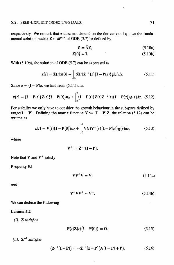
5.2. SEMI-EXPLICIT INDEX Two DAEs 71

respectively. We remark that z does notdepend on the derivative of q. Let the funda­mental salution matrix ZE mnxn of ODE (5.7) be defined by

Z=ÀZ, Z(O) =I.

With (5.10b), the salution of ODE (5.7) can be expressedas

(5.10a)

(5.10b)

z(t) = Z(t)z(O) +I Z(t)z-t (s){I- P(s))g(s)ds. (5.11)

Since z =(I P)z, we find from (5.11) that

z(t) =(I- P(t})Z(t){I- P(O))u0 +I (I P(t))Z(t)z-1 (s){I- P(s))g(s)ds. (5.12)

Por stability we only have to consider the growth behaviour in the subspace defined by range(I- P). Defining the matrix function V:= (I- P)Z, the relation (5.12) can be writtenas

z(t) = V(t)(I- P(O))uo +I V(t)V+(s)(I P(s))g(s)ds, (5.13)

where

v+ := z-1(1- P).

Note that V and v+ satisfy

Property 5.1

vv+v=v, (5.14a)

and

v+vv+=v+. (5.14b)

We can deduce the following

Lemma5.2

(i). Z satisfies

P(t)Z(t)(I- P(O)) = 0. (5.15)

(ii). z-l satisjies

(z-1 (1 P))·=-Z-1(1-P)(A(I P)+P). (5.16)

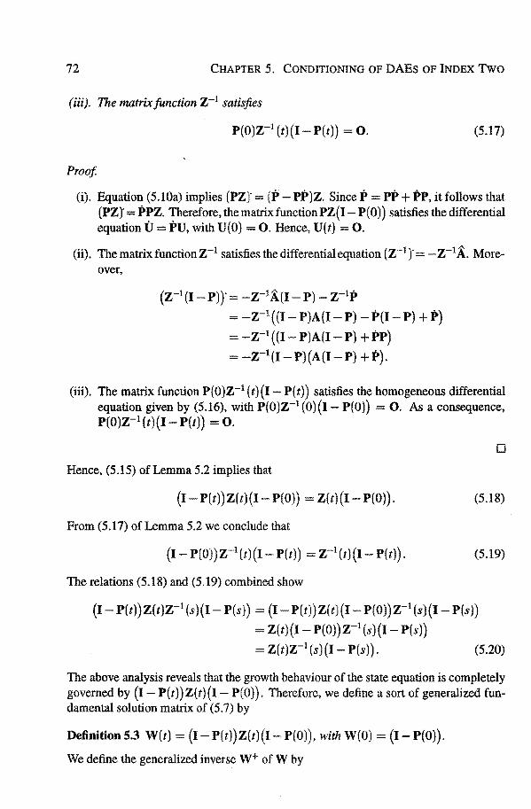
72 CHAPTER 5. CONDITIONING OF DAES OF INDEX TWO

(iii). The matrixjunction z-t satisfies

P(O)z-t (t)(I- P(t)) = 0. (5.17)

Proof

(i). Equation (5.10a) implies (PZ)" = (P- PP)Z. Since P = PP + PP, it follows that (PZJ = PPZ. Therefore, the matrix function PZ(I- P( 0)) satisfies the differential equation iJ= PU, with U(O) = 0. Hence, U(t) = 0.

(ii). Thematrixfunctionz-t satisfies the differentialequation (z-t )' = -z-t À. More­over,

(z-1(1-P))"= -z-1À(I- P)- z-Ip

= -z-1((I- P)A(I- P)- P(I- P) + :P) = -z-1((1- P)A(I- P) + PP)

-z-t (I- P){A(I- P) + P).

(iii). The matrix function P(O)z-t (t)(I- P(t)) satisfies the homogeneons differential equation given by (5.16), with P(O)z-1 (O)(I- P(O)) = 0. As a consequence, P(O)z-t (t)(I- P(t)) = 0.

D

Hence, (5.15) of Lemma 5.2 implies that

{I P(t))Z(t){I- P(O)) = Z(t){I- P(O)). (5.18)

From (5.17) of Lemma 5.2 we conclude that

(I-P(O))Z-1(t)(I-P(t)) =Z-1(t)(I-P(t)). (5.19)

The relations (5.18) and (5.19) combined show

(I- P(t))Z(t)z-t (s}(I- P(s}) (I P(t))Z(t)(I- P(O))z-1 (s)(I- P(s))

Z(t){I- P(O))z-t (s){I- P(s))

= Z(t)z-1 (s)(I- P(s)). (5.20)

The above analysis reveals that the growth behaviour of the state equation is completely govemed by (I- P(t)}Z(t}(I- P(O)). Therefore, wedefine a sort of generalized fun­damental salution matrix of (5.7) by

Definition 5.3 W(t) =(I- P(t))Z(t)(I- P(O)), with W{O) =(I- P(O)).

We define the generalized inverse w+ of W by

5.3. CONDITIONING POR ALMOST SINGULAR MATRIX CB 73

Definition5.4 w+(t) = (I-P(O))z-1(t)(I-P(t)).

With thesedefinitions both Wand w+ satisfyproperty 5.1. This results in the following

Theorem 5.5 The salution z ofthe state equation (5.7) can be written as

z(t) W(t)(I-P(O))uo+ I W(t)W+(s)(I-P(s))g(s)ds. (5.21)

Proof. The matrix function W satisfies W AW. Moreover, equation (5.20) yields that W(t)W+(t)(I- P(tl)g(t) =(I- P(t))g(t). D

From (5.21 ), wededuce the following estimates for the growth behaviour of zand x, i.e.

llzllco ~ Ktii(I P(O))xoll + Kz(II(I- P)plls + 11 (I P)AFqlls + 11 (I- P)Fqlls) (5.22)

and

llxllco ~ Kt(II{I-P(O))xoll + IIF(O)q(O)IIs)

+ Kz(ll (I- P)plls + 11 (I P)AFqlls + 11 (I- P)Fqlls) + IIFqllco. (5.23)

respectively, where the conditioning constants are defined as

Kt = max:{IW(t)l, t EI}, and, Kz = sup{[J~ IIW(t)W+ (s) 11' ds]llr, tE I},

(5.24)

where ~ + ; = 1. The conditioning constants K1 and Kz the effect of absolute errors due to absolute perturbations of the initial values and the inhomogeneities. The estimates above show that slight perturbations of p and q can yield large perturbations in the solution, if Kt. K2, or, more importantly, IIPII are large. Hence for DAEs not only the conditioning constants, but also the projectorPis very important. Furthermore, the algebraic variabie y satisfies

(5.25)

and therefore,

IIYIIco ~ 11 (CB)-1 11((11èllco + IICAIIco)llxllco + IICplloo + llqlloo). (5.26)

5.3 CONDITIONING FOR ALMOST SINGULAR MATRIXCB

In this section we study the conditioning of the IVP (5.1) for an almost singular matrix CB. Subsequently, differentiatingthe algebraic constraint (5.1b) and substituting the dy­namic equation (S.la) into it results in

0= (è+CA)x+CBy+Cp+q. (5.27)

74 CHAPTER 5. CONDITIONING OF DAES OF INDEX TwO

Consequently, the dynamic variabie is given by

y = -(CB)-1 ((è + CA)x + Cp + q). (5.28)

Substitution of this equation into the dynamic equation (5 .1 a) gives the underlying ODE (UODE)

x = ((I- P)A- Fè)x + (I- P)p- Fq. (5.29)

Por an almost singular matrix CB the conditioning of the index two IVP (5.1) is given by the following theorem.

Theorem 5.6 Consider the IVP (5.1). Let CB d, (el 0). Let CAB be nonsingular with all eigenvalues bounded away from zero. Assume that the DAE is stable. Let the matrix coefficients A, B and C vary slowly. Then the conditoning of this IVP is given by the estimates

and

llxll ::::; ~<tlx(O)I + ~<ziiPII + IIB(CAB)-1 11 (IICpll + ~tiCp(O)I + e~zi!Cpll)

+ IIB(CAB)-1 11(11ètll +~tlêJ(O)I) +e~ziiB(CAB)-1 1111iill (elO), (5.30)

llyll::::; ~ziiCAIIIx(O)I +~ziiCpll +~zlliill (el 0). {5.31)

The conditioning constants are dejined by

Kt := max{ 11 exp( -e-1 BCAt) 11, 0 ::::; t ::::; T} I

~~ := max{ 11 exp( -e-1CABt) 11, 0::::; t::::; T} I

Kz sup{J:IIexp(-e-1BCA(t-r))lldrl O:::;t:::;T}, and (5.32)

~z := e-1 sup{r 11 exp(-e-1CAB(t- rJ) 11 drl 0::::; t::::; T}.

Proof. Let CB =el, (el 0). The equations (5.29) and (5.28) can be rewritten as

x= ((I -e-1BC)A- e-1Bè)x +(I -e-1BC)p- e-1Bq, (5.33)

and

y ((è + CA)x +Cp+ êJ)~ (5.34)

respectively. As in the proof of Theorem 4.6 one can see that, in the initiallayer, it is sufficiently general to consider the following simpter constant coefficient ODE for x, i.e.

(5.35)

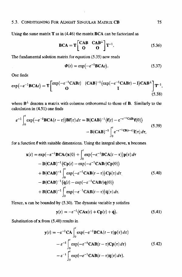
5.3. CONDITIONING POR ALMOST SINGULAR MATRIX CB 75

Using the samematrixTas in (4.46) the matrix BCA can be factorized as

BCA = T [C~B C~.l J T-1. (5.36)

The fundamental solution matrix for equation (5.35) now reads

tl>(t) = exp( -s-1BCAt). (5.37)

Onefinds

( -1BCA) T[exp(-s-1CABt) (CAB)-1(exp(-c1CABt)-I)CABJ.J,.._1 exp -s t = 0 1 ... '

(5.38)

where B.l denotes a matrix with columns orthorrormal to those of B. Similarly to the calculation in (4.51) one finds

s-1 I exp( -s-1 BCA(t- -r))Bf( r) d-r = B( CAB)-1 (f(t) e-e-ICABtf(O))

-B(CAB)-1 I: e-e-ICB(t-'rlf(r)dr,

fora function fwith suitable dimensions. Using the integral above, x becomes

x(t) = exp(-s-1BCAt)x(O) +I exp(-c1BCA(t r))p(r)dr

- B(CAB)-1 (Cp(t)- exp( -s-1CABt)Cp(Ol)

(5.39)

+ B(CAB)-1 I exp( -s-1CAB(t r))Cp{r)dr, (5.40)

- B(CAB)-1 (q(t) -exp(-s-1CABt)q(O))

+B(CAB)-1 I exp(-s-1CAB(t ï:))q(t')dr.

Hence, x can be bounded by (5.30). The dynamic variabie y satisfies

y(t) = -s-1 (CAx(t) + Cp(t) + q). (5.41)

Substitution of x from (5.40) results in

y(t) = -s-1CA I: exp(-s-1BCA(t- r)p(r)dr)

- s-1 I exp( -s-1CAB(t- r)Cp(r) dr) (5.42)

- s-1 t exp( -s-1CAB(t r)q(-r) dr).

76 CHAPTER 5. CONDITIONING OF DAES OF INDEX TWO

Since

CAexp(-C1BCAt) = exp(-e-1CABt)CA,

the resulting growth behaviour ofy is given by (5.31). D

Remark 5.7 The stability assumptions of Theorem 5.6 imply that all eigenvalues Ài of CAB satisfy 0 « Ài < M, fora constantMof moderate size. Therefore, tc1 = 1 and similarly for R1. Further, the conditioning constant 1(2 is of order of magnitude one.

Remark 5.8 Equation (5.30) shows that the matrix CAB plays an important role in the conditioning of x. N ote that this is the same matrix which de termines whether the sys­tem (5.1) with CB = 0 bas index three.

Remark 5.9 This theorem shows that x depends on the first derivative of q. Further, y depends on q and on ij_ as well.

As in the index one case (see Chapter 4) the e-1 effect is removable in the case that the matrix pencil (Ä, B) is regular forel 0, since this implies that the DAE is closetoa DAE of higher index. Again for problems with a singular matrix pencil (Ä, B) the sta­bility constants might be dominated by e-1 (el 0). Such a system is considered in Ex­ample 5.12 on page 79.

See Examle 6.9 for a mechanical example of such a system.

5.4 PERTURBATIONS OF THE COEFFICIENTS

Por DAEs of index two or higher it is important to consider not only the influence of perturbations of the initial values and the inhomogeneities, but it is also crudal to study the effect of perturbations of the coefficient matrices. Por ODEs and DAEs of index one the perturbations in the homogeneaus terms can be regarded as an inhomogeneity of the original IVP. From that analysis one can conclude that a well-conditioned IVP remains reasonably conditioned if the coefficient matrix is perturbed only slightly. For DAEs, however it is not as straightforward as that, because the state ODEs are derived only af­ter some matrix inversions have been dealt with. This implies that DAEs might be very sensitive to perturbations of the coefficients. In the remainder of this section we shall therefore consider the effect of perturbations of the coefficients A, B and C as well. From the original index two DAE (5.1a),(5.1b) we have derived the state ODE (5.7). lts fun­damental salution matrix Z satisfies (5.10), i.e.

• A

Z =AZ, Z(O) =I.

Slight perturbations of the coefficient matrices A, B, and C yield the following ODE for the corresponding perturbed fundamental salution matrix Z

5.4. PERTURBATIONS OF THE COEFFICIENTS

where

&À= (I- P)öA -&PA- (öP)' + h.o.t.

In the constant coefficient case this gives in first order approximation

&À ~ (I- P)öA- &PA.

Therefore, the perturbation óA can be large if A or P are large. Hence,

Z(t) = Z(t) +I Z(t)z-1 (s)öA(s)Z(s)ds

77

Z(t)(I+ I z-1(s)G(s)Z(s)ds-I z-1(s)H(s)Z(s)ds). (5.43)

Here, the perturbations G and H are defined by

G(t) :={I- P(t))öA(t)

and

H(t) := öP(t)A(t),

respectively. The perturbation G is of concern if the problem is ill-conditioned in the sense that P is skew. The perturbation H may be of concern even when the problem is well-conditioned. Compare relation (5.43) with solution (5.12). Since (I P)G G, the influence of the second term on the right hand side of (5.43) can be considered to be an additive perturbation, i.e. a perturbation caused by the force function g in equa­tion (5.12). Hence, the contribution of this perturbation is already controlled by the ad­ditive perturbations ( cf. ( 5.12)). For the perturbation H this will not hold in general, since (I- P)H =/= H. When H is large, Z may differ substantially from Z. Since H will gen­erally not be in the subspace defined by range(I- P), the difference betweenZand Z may not be controlled by equation (5.12) implying that the perturbed solution may prop­agate in the wrong subspace. This implies that the perturbed solution z may differ very much from the unperturbed solution z. From the above, we can draw the following con­clusions:

• The perturbation G is of concern if the problem is ill-conditioned in the sense that Pis skew. The stability of the solution can change because of G. The fundamental solution of the perturbed problem, however, will propagate in the same subspace as the unperturbed solution.

• The perturbation H may be of concern even when the problem is well-conditioned and it may also cause a change in the stability behaviour of the solution. However, in this case the perturbed solution might propagate in the wrong directions.

The following theorem shows the possible dramatic influence of perturbations of B and C on the stability behaviour of the DAE when P is large in norm.

78 CHAPTER 5. CONDITIONING OF DAEs OF INDEX TWO

Theorern 5.10 Consider the constant coefficient index two DAE (5.1a), (5.1b). Assume that CB = d, (s l 0). Let (I-P)A have bounded negative nontrivial eigenvalues. Per­turbations of the matrices B and C, say B = B + &B and ë = C + &C, may lead to a shift of order 8/s in the eigenvalues of(l- P)A, where II&BII <9(8) and likewisefor II&CII.

Proof The perturbations result in

P=P+&P,

where

&P = (B +&B)((C +&C){B +&B)r1 (C +&C)- s-1BC

= s-1(B +&B)(I +8-1C&B + e-1&CB +8-1&C&B)-1(C +&C) -8-1BC.

Let &B and &C be small enough so that

Th en

max{lls-1C&BII, lle-1&CBII, II8-1&C&BII} = 1J, (17 l 0).

&P = s-1(B +&B){I- s-1e&B -8-1&CB + C>(r,Z)}(C +&C)- 8-1BC

= s-1B&C + 8-1&BC + C>(qje).

0

The theorem above implies that perturbations of the coefficients of the order 8 may change the stability of the system dramatically when 8 is of the same order of magnitude as 8.

However, it is not unreasonable to think of much larger perturbations 8 in practice, e.g. if one. considers a linearization process for a nonlinear DAB. In the remainder of this section we will consider the influence of perturbations of either one of the coefficient matrices A, B, or C, in order to illustrate the analysis above. First, we study the effect of perturbations of A; so we consider the perturbed DAB

subject to

i(t) Á(t)x(t) + B(t)y(t) + p(t),

o = C(t)x(t) + q(t),

x(O) io,

(5.44a)

(5.44b)

(5.44c)

where Á = A + &A and io = xo + &xo. For ha ving consistent initia! values x0 we need C(O)&xo = 0, i.e. (I- P(Ol)&xo &x0• This implies that x0 has to be of the form (5.4).

This leads to the following perturbed state ODE

~={(I- P)Á P)z +(I- P)p (I- P)(ÁF- F)q

(À+ (I- P)&A)z +(I P)(g- &AFq). (5.45)

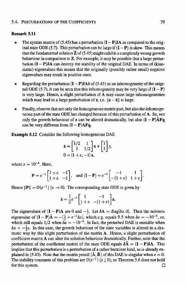
5.4. PERTURBATIONS OF THE COEFFICIENTS 79

Remark 5.11

• The system matrix of (5.45) has a perturbation (I P)8A as compared to the orig· inal state ODE (5.7). This perturbation can be large if (I P) is skew. This means that the fundamental salution Z of ( 5 .45) might exhibita completely wrong growth behaviour in comparison to Z. Por example, it may be possible that a large pertur­bation (I - P)8A can destray the stability of the original DAE. In terms of (kine­matic) eigenvalues this means that the originally (possibly rather small) negative eigenvalues may result in positive ones.

• Regarding the perturbation (I- P)&Az of (5.45) as an inhomogeneity of the origi­nal ODE (5.7), it can beseen that this inhomogeneity may be very large if (I P) is very large. Hence, a slight perturbation of A may cause large inhomogeneities which may leadtoa large perturbation of z, i.e. llz zll is large.

• Finally, observe that not only the homogeneaus matrix part, but also the inhomoge­neous part of the state ODE bas changed because of this perturbation of A. So, not only the growth behaviour of z can be altered dramatically, but also (I- P)ÁFq can be very different from (I- P)AFq.

Example 5.12 Consider the following homogeneaus DAE

. [1/2 1 J [1] x= 1 1/2 x+ 1 y,

0 = [1 + s, -1] x,

where s = 1 o-4 • Here,

P=s-1 [!!: =U· and(I P) [

-1 1 J -(l+s) l+e ·

Hence IIPII = e:>(s-1 ) (s--+ 0). The corresponding state ODE is given by

~8-1 [1 ~s -(1 +s)]z.

The eigenvalues of (I P)A are 0 and -t. Let &A = diag[8a, 0]. Then the nonzero eigenvalue of (I P)Á = -(! + e-18a), which e.g. equals 9.5 when &a= -10-3, or, which still equals 1/2 when &a = -1 o-4• In fact, the perturbed DAE is unstable when &a < -te. In this case, the growth behaviour of the state variables is altered in a dra­matic way by this slight perturbation of the matrix A. Hence, a slight perturbation of coefficient matrix A can alter the salution behaviour dramatically. Further, note that the perturbation of the coefficient matrix of the state ODE equals öA = (I- P)&A. This implies that this perturbation is a perturbation of a rather harmless kind, as is already ex­plainedin (5.43). Note that the matrixpencil (Ä, B) ofthis DAEis singularwhen s = 0. The stability constants ofthis problem are C>(s-1 ) (s 1 0), so Theorem 5.6 does not hold for this system. 0

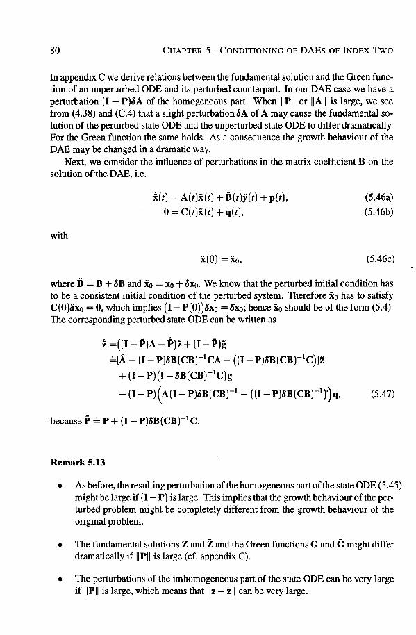
80 CHAPTER 5. CONDITIONING OF DAEs OF INDEX Two

In appendix C we derive relations between the fundamental salution and the Green func­tion of an unperturbed ODE and its perturbed counterpart. In our DAB case we have a perturbation (I- P)8A of the homogeneaus part. When IIPII or IIAII is large, we see from (4.38) and (C.4) that a slight perturbation8A of A may cause the fundamental so­lution of the perturbed state ODE and the unperturbed state ODE to differ dramatically. For the Green function the same holds. As a consequence the growth behaviour of the DAB may be changed in a dramatic way.

Next, we consicter the influence of perturbations in the matrix coefficient Bon the salution ofthe DAB, i.e.

with

i(t) = A(t)x(t) + B(t)y(t) + p(t),

o = C(t)x(t) + q(t),

x(O) = io,

(5.46a)

(5.46b)

(5.46c)

where B = B + 8B and x0 = x0 + 8x0 • We know that the perturbed initia! condition has to be a consistent initia! condition of the perturbed system. Therefore io has to satisfy C(0)8x0 = 0, which implies (I- P(O) )8xo = 8xo; hence io should be of the farm (5.4). The corresponding perturbed state ODE can be written as

i =((I -P)A- P)z +(I- P)g

~[À- (I- P)8B(CB)-1CA- ((I- P)8B(CB)-1C)1z

+ (I-P){I-8B(CB)-1C)g

- (1-P)(A(I-P)&B(CB)-1 - ((I-P)8B(CB)-1)Jq. (5.47)

because P ~ P +(I- P)8B(CB)-1C.

Remark5.13

• As before, the resulting perturbation of the homogeneaus part of the state ODE (5 .45) might be large if (I- P) is large. This implies that the growth behaviour of the per­turbed problem might be completely different from the growth behaviour of the original problem.

• The fundamental solutions Z and Z and the Green functions G and G might differ dramatically if IIPII is large (cf. appendix C).

• The perturbations of the imhomogeneous part of the state ODE can be very large if IIPII is large, which means that llz- zll can be very large.

5.4. PERTURBATIONS OF THE COEFFICIENTS

As a consequence, the perturbed solution x satisfies

x z+Px = z- Fq- (I- P)8B(CB)-1q.

Hence, due to the arguments above x and x might differ dramatically.

81

(5.48)

Example 5.14 Again, consider Example 5.12. Now, the coefficientmatrixB is perturbed slightly, say

B := [1i&l. Then

- - - -1 1 [ -(1 + 8) 1 J (I-P)=I-B(CB) C= s-8 -(1+e)(1+8) l+s

Ä -A= (I-P)A 1 [ 8-1 1+28 ] 2(8 s) (1 + s)(8 1) (1 + s)(l + 28) '

with nonzero eigenvalue 382{;!.?}8

• For 8 = -510-s this nonzero eigenvalue of the per­turbed system is equal to 1.66710-J, which implies that the originally stabie system is perturbed into an unstable one by a small perturbation of the matrix B. Note further, that (I - P )Ä = Î. This means that we deal with a perturbation of the state ODE which is of the samekind as the second term of (5 .43) and from (5 .43) we know that this perturbation may be controlled already. D

Next we study the effect of perturbations of the matrix coefficient C on the salution of the DAB system, i.e. we consider the perturbed problem

subjectto

where ë = C +8C and

i(t) = A(t)x(t) + B(t)y(t) + p(t),

o = ë(t)x(t) + q(t).

x(O) =xo,

(5.49a)

(5.49b)

(5.49c)

xo = x0 + ÓXo. Now, fora consistent initial condition of the perturbed system io should satisfy ë(O)óXo 0. For the first order terros this means that C(O)x0 + óC(O)xo = 0. Again, this implies that io should be of the form (5.4). In this case one finds for the perturbed projector P

P ";, P+FóC(I- P).

Then, the corresponding perturbed state ODE can be written as

i ={(I- P)A- P)z +(I- P)g

=[A- FóC(I- P)A- (FöC(I- P))'lz

+{I- FóC)(I- P)g +(I- P)(AFóCF- (FóCF)')q. (5.50)

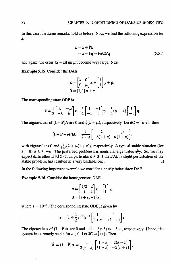
82 CHAPTER 5. CONDITIONING OF DAES OF INDEX TWO

In this case, the same remarks holdas before. Now, we find the following expression for i

x=z+Pi =z Fq-FóCFq (5.51)

and again, the error llx- ill might become very large. Next

Example 5.15 Consider the DAE

x=[~ Z]x+[i]y+p, 0 = [1, l]x+q.

The corresponding state ODE is

- z+-1 [ À _,_"] 1 [ 1 2 -À ti 2 -1

-1] 1 [ 1 J 1 p + 4 (f-1, - À) -1 q.

The eigenvalnes of (I- P)A are 0 and Î(À + J-t), respectively. Let&C =[.se o], then

1 [ À _,_" J (I- P-óP)A = 2 + 8 -À(l +e) ,_"(1 + e) ,

with eigenvalnes 0 and z!e (À + ,_" ( 1 + e)), respectively. A typical stabie situation (for

e = 0) is À ~ -f-1,. The perturbed problem has nontrivial eigenvalue z":.s· So, we may expect difficulties if jÀj » 1. In particular if À » 1 the DAE, a slight perturbation of the stabie problem, has resulted in a very unstable one. D

In the following important example we consider a near1y index three DAE.

E:xample 5.16 Consider the homogeneaus DAE

i = [ 1 {2 î J x + [iJ y,

0 = [1 +e, x,

where e w-4 • The corresponding state ODE is given by

( 1 -1 -1 [ 1 -1 J 1 + Ï 8 )8 1 + 8 - ( 1 + 8) z.

The eigenvalnes of (I P)A are 0 and -(1 + te-1) ~ -5w, respectively. Hence, the system is extremely stabie for 8 l 0. Let &C = [ o .s] • Then

"' - 1 [ 1-8 2(8- 1) J A=(I-P)A=2(e+8) (1+8) -2(1+8)'

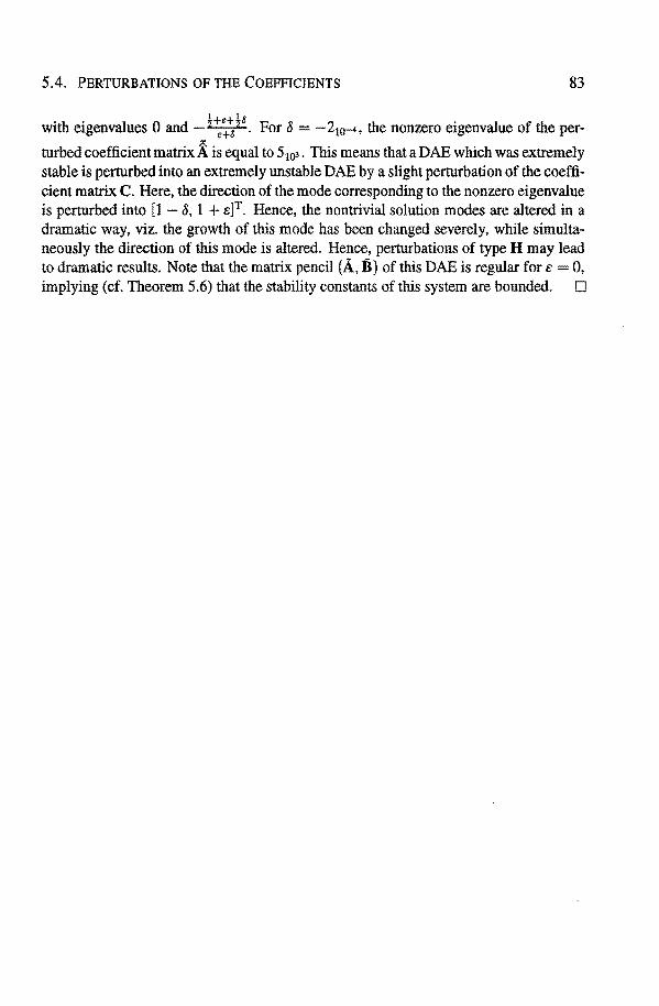
5.4. PBRTURBATIONS OF THB COBFFICIBNTS 83

with eigenvalnes 0 and - !~:~ !8• For 8 -210-4, the nonzero eigenvalue of the per­

turbed coefficient matrix i is equal to 5103 • This means that a DAE which was extremely stabie is perturbed into an extremely unstable DAE by a slight perturbation of the coeffi­cient matrix C. Here, the direction of the mode corresponding to the nonzero eigenvalue is perturbed into [1 - 8, 1 + s]T. Hence, the nontrivial salution modes are altered in a dramatic way, viz. the growth of this mode bas been changed severely, while simulta­neously the direction of this mode is altered. Hence, perturbations of type H may lead to dramatic results. Note that the matrix pencil (Á, B) of this DAE is regular fors 0, implying (cf. Theorem 5.6) that the stability constauts of this system are bounded. D

84 CHAPTER 5. CONDITIONING OF DAES OF INDEX Two

6 REGULARIZATION AND

STABILIZATION

The study of numerical methods for solving DAEs of higher index is the subject of this chapter. In Chapter 3 we have shown that numerical methods for solving stiff ODEs are in general only convergent for index one systems and a loss ofthe approximation order may occur in the algebraic variables. Fortunately, BDF methods converge for some im­portant classes of DAEs, e.g. systems in Hessenberg forms. However, BDF codes, using variabie step-sizes and variabie order, still do not work properly. The equations of mo­tion for multibody systems are generally index three. In order to solvethese equations by BDF codes one has to reduce the index to one by successive differentiations of the con­straints. This, howevèr, results in numerical solutions drifting away from the constraints, as will be shown in Section 6.1. Th alleviate this effect of drifting away from the con­straints, special techniques for solving higher index DAEs, and equations of motion for multibody systems in particular, have to be developed. In Section 6.1 such methods are studied. Discretization of higher index DAEs by BDF methods yields ill-conditioned it­eration matrices. The effects of this ill-conditioning on the numerical solution of DAEs is analysed inSection 6.2; we show that it can affect the numerical solution badly. For DAEs that are nearly higher index, as considered in the Chapters 4 and 5 this effect tums out to be even worse. A metbod is given to reduce the effects of ill-conditioned iteration matri­ces on the approximation ofthe solution of DAEs of (nearly) higher index. The conse­quences for variabie step-size and variabie order BDF codes are elaborated inSection 6.3. We will show that these ill-conditioning effects can be remedied in a way allowing for the numerical solution of DAEs in higher index fonn directly. In Section 6.4 applications to multibody systems are shown. In particular, the numerical solution of these mechanica! systems using a projector technique appears to be preferable.

86 CHAPTER 6. REGULARIZATION AND STABILIZATION

6.1 SOLUTION TECHNIQUES FOR HIGHER INDEXDAEs

In this section integration schemes for the equations of motion generated by multibody systems are discussed. In Sections 3.2 and 3.3 the numerical solution of DAEs by mul­tistep and Runge-Kutta methods is studied. These methods can generally not be applied to higher index ( v 2: 2) DAEs, since most of them are convergent for index one problems only. Another problem is the loss of accuracey for the algebraic variables. This causes standard techniques of error estimation and step-size selection to fail. These problems can be avoided by differentlating the DAEs v 1 times with respect to time. Such index­reduced system can then be solved numerically by multistep or Runge-Kutta methods, for example. This approach gives rise to two problems. First, the numerical solution of the index-reduced system does not fulfill the original constraints every step: hence due to error propagation, the numerical solution tends to drift away from the algebraic con­straillts (cf. [27]). Secondly, the stability ofthe DAE with respect to perturbations in the solution may change due to the index transformation (cf. [28]). To show the effect of this index rednetion we again consider the pendulum studied in the Examples 2.1 through 2.3.

Example 6.1 Let us choose 1 = 1, m 1 and g such that the pendulum swings with a period T 2, i.e. g = 4/3 · 13.751• The initial positions x(O) 0, y(O) = 1 and <p(O) = rr/2, together with the inital veloeities x(O) = y(O) = cp(O) 0 are consistent as can easily be seen. We compute the numerical solution over 50 periods with a toler-

8p

t

' Position Constraints

8v Velocity Constraints

0.8 0.01 ..

1 .....

0.6 0.008

... 0.006 ......

0.4 0.004

0.2

0 0 50 100 50 100

-t -t Figure 6.1 Resulting drift for TOL = 10-4• The dotted lines represent the ab­solute deviations from the position constraint x -l cos <p = 0 ( denoted by op) and its derivative (denoted by ov). whereas the deviations from the position constraint y - l sin <p = 0 and its derivative are represented by the solid lines.

ance TOL = 10-4. Figure 6.1 shows that the numerical solution of the reduced DAE drifts away from the constraints. The resulting global errors at t = 100 are given by ex:= lx(t) -xnl =0.16 ·101 , e, =0.83, e'fl =0.99, eÀ1 = 0.20-102 andeÀ2 =0.30·102 ,

used g = 4/3 · 13.7503716360407457 which has been computed using elliptic integrals.

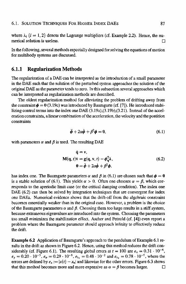
6.1. SOLUTION TECHNIQUBS FOR HIGHER INDEX DAEs 87

where Ài (i= 1, 2) denote tbe Lagrange multipliers (cf. Example 2.2). Hence, tbe nu­merical solution is useless. 0

In the following, several metbods especially designed for solving tbe equations of motion for multibody systems are discussed.

6.1.1 Regularization Methods

The regularization of a DAE can be interpreted as tbe introduetion of a small parameter in tbe DAE such tbat tbe solution of the pertorbed system approaches tbe solution of tbe original DAE as tbe parameter tends to zero. Intbis subsection several approaches which can be interpreted as regularization metbods are described.

The oldest regularization metbod for alleviating tbe problem of drifting away from tbe constraintt/1 = 0 (3.19c) was introduced by Baumgarte (cf. [7]). He introduced stahi­lizing control terros into tbe index one DAE (3.19a),(3.19b),(3.21). Insteadof tbe accel­eration constraints, a linear combination of tbe acceleration, the velocity and tbe postirion constraints

(6.1)

witb parameters a and fJ is used. The resulting DAE

q=v, • T. M(q, t)v = g(q, v, t) -1/Jql, (6.2)

0 ÎÎ' + 2aip + pzq,.

bas index one. The Baumgarte parameters a and fJ in (6.1) are cho.sen such that fjJ 0 is a stabie solution of (6.1). This yields a > 0. Oftenone chooses a= {J, which cor­responds to tbe aperiodic limit case (or tbe critical damping condition). The index one DAE (6.2) cantben be solved by integration techniques tbat are convergent for index one DAEs. Numerical evidence shows tbat tbe drift-off from the algebraic constraint becomes essentially weaker tban in the original case. However, aproblem is tbe choice of the Baumgarte parameters a and {J. Choosing tbem too large results in a stiff system, becanse extraneous eigenvalnes are introduced into tbe system. Choosing tbe parameters too small minimizes tbe stabilization effect. Aseher and Petzold (cf. [4]) even report a problem where tbe Baumgarte parameter should approach infinity to effectively reduce the drift

Example 6.2 Application ofBaumgarte's approach to tbe pendulom ofExample 6.1 re­sults in tbe drift as shown in Figure 6.2. Hence, using tbis metbod reduces tbe drift con­siderably (cf. Figure 6.1). The resulting global errors at t = 100 are ex= 0.31 · w-4, ey = 0.20. w-3' erp 0.29 . w-3' eÀl = 0.48 . w-z and eÀ2 = 0.78 . w-s' where tbe errors aredefined by ex:= lx(t) -xnl and likewise forthe otbererrors. Figure 6.3 shows tbat tbis metbod becomes more and more expensive as a = fJ becomes larger. 0

88 CHAPTER 6. REGULARIZATION AND STABILIZATION

4 x 10-

4 Position Constraints 8p

I 2 . .

: ::

5 x 10-4 Velocity Constraints

8v

t 4

3

.. 2 ..

50 100 -t

50 100 -t

Figure 6.2 Resulting drift using Baumgarte's approach with a = f3 = 6, which seems to be a more or less optimal choice for a, for TOL = 10-4. The dotted lines represent the absolute deviations from the position constraint x -l cos qJ = 0 ( denoted by ó p) and its derivative ( denoted by äv ), whereas the deviations from the position constraint y l sin rp 0 and its derivative are represented by the solid lines.

5.5.--~--~--,

10 1og(# steps) t 5

4.5

4~------3.51....--------'

0 2 3

-10 loga

Figure 6.3 Number of steps as tunetion ofthe Baumgarte parameter a {3, for TOL = 10-4 and t 100. The straight line denotes the number of steps needed for solving the projection metbod (6.12) (see Subsection 6.1.3).

Other regularization techniques were proposed by Lötstedt, Knorrenschild and Hank.e and have been compared by Eich and Hanke (cf. [22]), who showed that these methods are actually very similar. Lötstedt (cf. [22]) introduced penalty functions which lead to the equation

Mij g-e-1K.

Applying Knorrenschild's approach yields

Mq =g-fi!.A.,

0 = ,P(q + (e + J,t,)q + JkBM-1 (g -f/IT.A.)),

while Hank.e's regularization technique results into

q=v+Jkv, Mv = g(q, V, t) t~J!.A.,

0 = t/J{q + eq + J,t,EM-1 (g -f/IT.A.)).

(6.3)

(6.4)

(6.5)

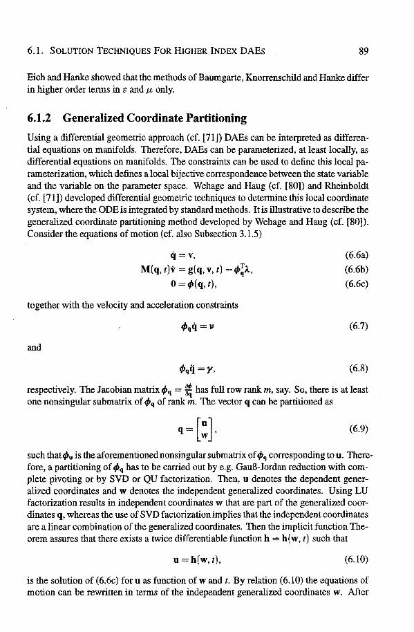
6.1. SOLUTION TECHNIQUES POR HIGHER INDEX DAES 89

Eich and Ranke showed that the methods of Baumgarte, Knorrenschild and Ranke differ in higher order terms in e and I" only.

6.1.2 Generalized Coordinate Partitioning

Using a differentlal geometrie approach (cf. [71]) DAEs can be interprered as differen­tlal equations on manifolds. Therefore, DAEs can be parameterized, at least locally, as differentlal equations on manifolds. The constraints can be used to define this local pa­rameterization, which defines alocal bijective correspondence between the state variabie and the variabie on the parameter space. Wehage and Haug (cf. [80]) and Rheinboldt (cf. [71.]) developed differentlal geometrie techniques todetermine this local coordinate system, where the ODE is integrated by standard methods. It is illustrative to describe the generalized coordinate partitioning metbod developed by Wehage and Haug (cf. [80]). Considerthe equations of motion (cf. also Subsection 3.1.5)

q=v, M(q, t)v = g(q, v, t) -t/J!À,

0 =t/J{q, t),

together with the velocity and acceleration constraints

and

(6.6a)

(6.6b)

(6.6c)

(6.7)

(6.8)

respectively. The Jacobian matrix t/Jq = ~ has full row rank m, say. So, there is at least one nonsingular submatrix of t/Jq of rank m. The vector q can be partitioned as

q=[:]. (6.9)

such thatt/Ju is the aforementioned nonsingular submatrix of t/Jq corresponding to u. There­fore, a partitioning of t/Jq has to be carried out by e.g. GauB-Jordan reduction with com­plete pivoting or by SVD or QU factorization. Then, u denotes the dependent gener­alized coordinates and w denotes the independent generalized coordinates. U sing LU factorization results in independent coordinates w that are part of the generalized coor­dinates q, whereas the use of SVD factorization implies that the independent coordinates are a linear combination of the generalized coordinates. Then the impHeit functlon The­orem assures that there exists a twice differentiable function h = h ( w, t) such that

u= h(w, t), (6.10)

is the solution of ( 6.6c) for u as function of w and t. By relation ( 6.1 0) the equations of motion can be rewritten in terms of the independent generalized coordinates w. After

90 CHAPTER 6. REGULARIZATION AND STABILIZATION

elimination of the Lagrange multipliers, the equations of motion can be expressed as an ODE for the coordinates w, i.e.

w=s,

M(w, t)s = ~{w, s, t). (6.11)

This ODE can be solved numerically by standard methods. Given the complexity of the matrix M and the vector~ of ( 6.11) as functions of wand s, direct discretization of ( 6.11) would be very complicated and impracticable. Therefore, one solves q = [üT, wT]T from the DAE (6.6a), (6.6b), (6.7). Now w can be integrated by any explicit ODE solver to find wand w. Afterwards u and ü can be obtained by solving (6.6c) and (6.7), respec­tively. This can be continuedas long as the partitioning ( 6.9) does not need to be changed. However, if f>u becomes ill-conditioned, then the generalized coordinates q should be repartitioned, which is a major disadvantage of this method. Haug and Yen (cf. [47]) also developed an impHeit OAE solver based on generalized coordinate partitioning.

6.1.3 Projection Methods

Drift-offfrom the constraints can be avoided by numerically solving a OAE with reduced index, combined with a projection such that the original constraints are satisfied. Eich et al. (cf. [21]) have shown that these projeedons can be divided into two classes, depend­ing on whether they rely on stahilizing projectionsof position and velocity variables (co­ordinate projection methods) or on projections of residuals of the differentlal equations (derivative projection methods).

Gear et al. ( cf. [34]) have introduced stahilizing Lagrange multipliers p,, say, to si­multaneously reduce the index and satisfy the position constraint and the velocity con­straint

q v-f>!p,,

M(q, t)v = g(q, v, t) f>!l,

0=</>(q,t),

0 = </>q(q, t)v- v.

(6.12)

A salution of (6.12) exists only ifthe additional stahilizing multipliers IL satisfy IL = 0. Hence, (6.12) and the original system have the same solution. OAE (6.12) has index two and can be integrated numerically. We have applied this projection metbod to the pendulum of Example 6.1.

Example 6.3 For a toleranee TOL = w-4 the deviation of the constraints is smaller than 0.44 . w-tS. The resulting errors at t 100 are ex = 0.13 . w-5 ' ey 0.16 . w-2 '

erp = 0.16. to-2 ' e~,.I 0.29. w-t and eÀ2 = 0.71 . w-4• Figure 6.3 shows that the num­ber of steps2 taken in this metbod is considerably smaller than in Baumgarte's approach.

0 2In the computation we used the sealing, of the local error estimates and the sealing of the error esti­

mates in the Newton iterations, as developed in Section 6.3

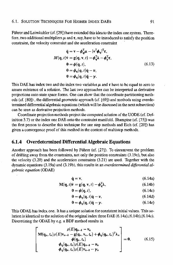
6.1. SOLUTION TECHNIQUES FOR HIGHER INDEX DAES 91

Führer and Leimkuhler ( cf. [29]) have extended this idea to the index one system. There­fore, two additional multipliers 1-L and 'E', say, have to be introduced to satisfy the position constraint, the velocity constraint and the acceleration constraint ·

q =V- cfJ!IL- [VTfJq]T'E',

M(q, t)v = g(q, V, t) -cfJ!l -cfJ;'E',

0 cfJ(q,t),

O=cfJq(q,t)q V,

0 =fJq(q, t)q- y.

(6.13)

This DAE has index two and the index two variables 1-L and 'E' have to be equal to zero to assure existence of a solution. The last two approaches can be interpreted as derivative projections onto state space forms. One can show that the coordinate partitioning meth­octs (cf. [80]), the differentlal geometrie approach (cf. [69]) and methods using overde­termined differentlal algebraic equations ( which will be discussed in the next subsection) can be seen as derivative projection methods.

Coordinate projection methods project the computed salution of the UODE (cf. Def­inition 3.7) or the index one DAE onto the constraint manifold. Shampine (cf. [75]) was the first person to describe this technique for one step methods and Eich ( cf. [20]) has given a convergence proof of this methad in the context of multistep methods.

6.1.4 Overdetermined Differential Algebraic Equations

Another approach has been followed by Führer (cf. [27]). To circumvent the problem of drifting away from the constraints, not only the position constraints (3.19c), but also the velocity (3.20) and the acceleration constraints (3.21) are used. Tagether with the dynamic equations (3.19a) and (3.19b), this results in an overdetermined differential al­gebraic equation (ODAE)

q=v,

M(q,t)v g(q,v,t)-cfJ!l.

0 cfJ(q,t),

O=cfJq{q,t)q -V,

0 =t/>q(q, t)q -y.

(6.14a)

(6.14b)

(6.14c)

(6.14d)

(6.14e)

This ODAE has index one. It has a unique solution for consistent initia! values. This so­lution is identical to the solution of the original index three DAE ( 6.14a),( 6.14b ),( 6.14c ). Discretizing the ODAE by e.g. a BDF method results in

p(E)qn-k -V,.

M(q,., t,.)p(E)v"_k- g(q,., v,., t,.) +t/>q(q,., t,.)1l" tf>(q,.,t,.) =0, (6.15)

fJq(q,., t,.)p(E)qn-k- V,. fJq(q,.,t,.)p(E)v"_k -y,.

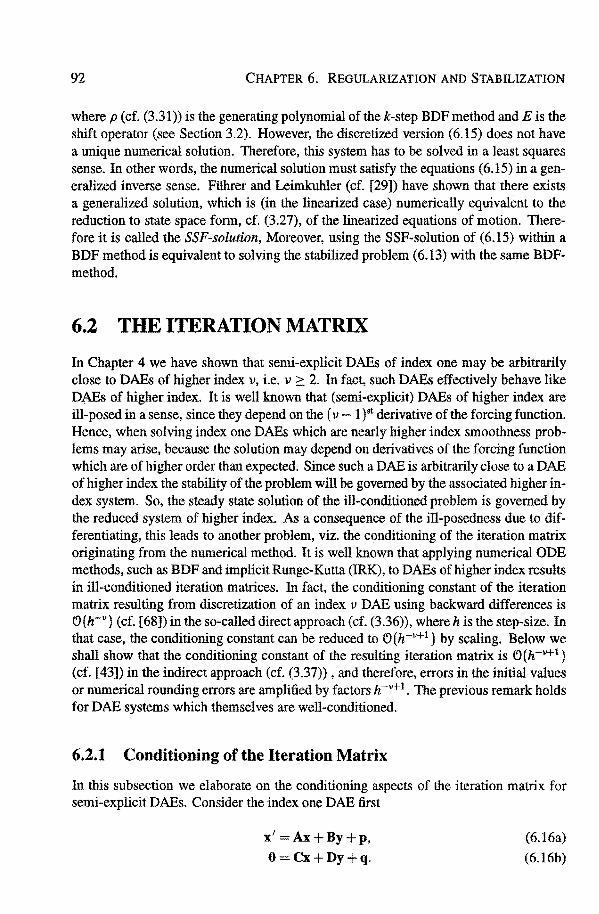
92 CHAPTBR 6. RBGULARIZATION AND STABILIZATION

where p (cf. (3.31)) is the generating polynomial ofthek-step BDF method and Eis the shift operator (see Section 3.2). However, the discretized version (6.15) doesnothave a unique numerical solution. Therefore, this system has to be solved in a least squares sense. In other words, the numerical salution must satisfy the equations (6.15) in a gen­eralized inverse sense. Führer and Leimkuhler (cf. [29]) have shown that there exists a generalized solution, which is (in the linearized case) numerically equivalent to the reduction to state space form, cf. (3.27), of the linearized equations of motion. There­fore it is called the SSF-solution, Moreover, using the SSF-solution of (6.15) within a BDF method is equivalent to solving the stabilized problem (6.13) with the same BDF­method.

6.2 THE ITERATION MATRIX

In Chapter 4 we have shown that semi-explicit DABs of index one may be arbitrarily close to DAEs of higher index v, i.e. v 2:: 2. In fact, such DAEs effectively behave like DAEs of higher index. lt is well known that (semi-explicit) DAEs of higher index are ill-posed in a sense, since they depend on the ( v- 1 )•t derivative of the forcing function. Hence, when solving index one DAEs which are nearly higher index smoothness prob­lems may arise, because the salution may depend on derivatives of the forcing function which are of higher order than expected. Since such a DAB is arbitrarily closetoa DAB of higher index the stability of the problem will be govemed by the associated higher in­dex system. So, the steady state salution of the ill-conditioned problem is govemed by the reduced system of higher index. As a consequence of the ill-posedness due to dif­ferentiating, this leads to another problem, viz. the conditioning of the iteration matrix originating from the numerical method. It is well known that applying numerical ODE methods, such as BDF and implicit Run ge-Kutta (IRK), to DAEs of higher index results in ill-conditioned iteration matrices. In fact, the conditioning constant of the iteration matrix resulting from discretization of an index v DAB using backward differences is e:>(h-v} (cf. [68]) in the so-called direct approach (cf. (3.36)), where h is the step-size. In that case, the conditioning constant can be reduced to e:>(h-v+1) by sealing. Below we shall show that the conditioning constant of the resulting iteration matrix is e:>(h-v+1) (cf. [43]) intheindirect approach (cf. (3.37)), and therefore, errors in the initial values or numerical rounding errors are amplified by factors h-v+l. The previous remark holds for DAB systems which themselves are well-conditioned.

6.2.1 Conditioning of tbe Iteration Matrix

In this subsecdon we elaborate on the conditioning aspects of the iteration matrix for semi-explicit DABs. Consicter the index one DAB first

x' Ax+By+p. 0 Cx+Dy+q.

(6.16a)

(6.16b)

6.2. THE ITERATION MATRIX 93

In the indirect approach, numerical ODE methods for the approximation of the solution of the DAE above will essentially involve an iteration matrix of the following form

·- [I -ÎiA -fis] hJt .- e n ' (6.17)

wheree.g. in thecase ofmultistepmethods Îi := hf30ja0 • Theinverse of hJ1 can becom­puted through LU-decomposition, i.e.

[ I 0] [I -hA -ÎiB J hJt =LU:= e(I- ÎiA)-1 I 0 fie{I- ÎiA)-1 S + n . (6.18)

Por u-1 weneed the inverse ofthe matrix fie(I- ÎiA)-1S + n. Let us first assume that the matrix n is such that

This implies that

-1 [ I+ Îi(A- sn-1e) fisn-1 J (hJtl = -n-1e(I + Îi(A sn-1e)) (I- fin-1es)n-1 + e>(h

2).

(6.20)

Notice the important role ofthe matrices n-te and A sn-te in the equation above. Hence, rounding errors proportional to the machine constant rJ be introduced both in x and in y, while solving this linear system. This means that such a DAE behaves as well conditioned as an ODE. Here and in the sequel the latter bas to be understood in an ab­solute (i.e. not relative) sense. If, on the other hand IID-1 11 is not small, problems arise. Por simplicity take D =el, (s ~ 0) (see also Section 4.3), then we find for small fixed Îi that

{Îie(I- ÎiA)-1S + nr1

=fi-t (est1 {I -ÎieAS(es)-1)

+ C>(Îi) + C>(e{h2 ), (s ~ 0), (6.21)

when the matrix es is well-conditioned and bounded away from zero. We thus find

_ 1 [ (I- P)(I + ÎiA(I P)) (I+ Îi(I- P)A)S(es)-1 J (hJt) = -fi-1 (es)-1e(I + ÎiA(I- P)) 1l-1(es)-1 (I- fieAS(es)-1) (6.22)

+ h.o.t., (e ~ 0),

where the projectorPis defined by P := S(es)-1e, cf. also Section 5.2. This implies that rounding errors proportional to rJ and T}h-1 may he introduced in the variables x and y, respectively. Here and in the sequel we assume that the (approximate) variables have a moderate norm, so that absolute and relative errors are qualitatively the same. Hence, we shall consider absolute "machine" rounding errors o rather than relative rounding errors C>(17) in our examples. The matrix (hJd-1 (cf. (6.22)) shows the ill-posedness, due to differentiation of the forcing function, of an index one DAE which is close to a DAE of higherindex (cf. Subsection 4.3).

94 CHAPTER 6. REGULARIZATION AND STABILIZATION

Example 6.4 Consider the index one DAE

x -y +sint,

0 =x-sy-cost,

subject to the initial condition x(O) = 2. On the interval [0, 10-3] we obtain from dis­cretization withEulerbackward Table 6.1, where ex:= lx(tn) -xnl. ey := ly(tn)- Ynl and drift IXn - EYn -cos tnl. i.e. the deviation from the constraint, for nh = T = 10-3

• In order to show the infl.uence of the rounding errors we introduce artificial absolute round­ing errors 8, say, with 8 e [4 · 10-5 ,6 · 10-5], into the system, where s was taken equal to 10-6 • lt is obvious that errors proportional to 8 are introduced into the state vari-

h ex ey drift 10-4 0.49. 10-4 0.75. 10-1 0.49 ·10-4

10-s 0.55 ·10-4 0.13. 10° 0.55 ·10-4

10-6 o.54. Io-4 0.14. 101 0.54 ·10-4

10-7 0.55 -10-4 0.30 ·101 0.58. 10-4

10-s 0.55 ·10-4 0.10. 10° 0.56-10-4 i

10-9 0.55 -10-4 0.35. 101 0.58. 10-4

Table 6.1 Results for the index two DAE ofExample 6.5 showing the h,-t effect in the algebraic variabie y.

able x. Note that from the first three rows of Table 6.1 it appears that the numerical ap­proximation of the algebraic variabie y has errors proportional to 8h.-t. Inthelast three rows, however, the resulting errors are proportional to 8e-1 ; this is explained in Subsec­tion 6.2.2. D

For a Hessenberg form DAE of index two

x' =Ax+By+p.

O=Cx+q. (6.24)

where CB is nonsingular, the resulting iteration matrix equals

[I-hA -hBJ hJz := C 0 . (6.25)

Performing LU-decomposition we find a similar expression as in ( 6.18), but with D = 0. When the matrix CB is well-conditioned and bounded away from zero the inverse of hJ2

is equal to (hJt)-1 (s --1 0) (cf. (6.22)). This means that the numerical solution of the index one DAE (6.16) behaves like a salution of the associated index two DAE (6.24). In Chapter 4 we have shown that this also holds for the exact solution. Rounding errors proportional to 11 and flh-1 are introduced in the variables x and y, respectively. This shows the ill-conditioning of a higher index DAE.

6.2. THE ITERATION MATRIX

Example 6.5 Consicter the following DAE of index two

i= -y+sint,

0 =x-cost,

95

subject to the initia! condition x( 0) = 1, y( 0) = 0. This DAE has solution x( t) = cos t, y(t) = 2sint. lntroducing artificial errors 8 E [4 · 10-5 , 6 · 10-5], into the system shows the inftuence of the rounding errors. On the interval [0, 1 o-3] we obtain from discretiza­tion with Euler backward the following table, where we use the following definitions: ex:= lx(tn) Xnl. ey := iy(tn)- Ynl and drift:= lxn- costnl, i.e. the deviation from the constraint, for nh = T = 10-3 • Table 6.2 shows that errors proportional to 8 appear in

h ex ey drift w-4 0.54 .w-4 o.57 .w-2 0.54 .w-4 w-s o.6o .w-4 0.62 ·10° o.6o .w-4 w-6 o.51. w-4 0.44 ·10° o.51 . w-4 w-1 o.59 .w-4 0.72 ·101 0.59-10-4

w-s o.54 .w-4 0.20 ·103 $54·10-4

w-9 o.58 .w-4 0.11. 105 0.58 .w-4

Table 6.2 Results for the nearly index two index one DAE ofExample 6.5 show­ing the 'h-1 effect in the algebraic variabie y.

the state varlablex whereas errors proportional to ofi-1 are introduced into the algebraic variabie y. 0

However, for CB =el, (e -t 0) (see also Section 5.3), (fiC(I- 'ÎiA)-1Br1

has to be computed. Por small fixed h we find that

(7iC(I-'ÎiA)-1Br1

=h-2(CAB)-1{I 'ÎiCA2B(CAB)-1)

+ (.') ( 1) + (.') (ej'Îi3 ), (e -t 0),

(6.27)

when the matrix CAB is well-conditioned and bounded away from zero. Hence,

(e-t 0}, (6.28)

implying that rounding errors proportional to 1'/Ji-1 and 17h-2 are introduced in the vari­ables x and y, respectively. Note that when CB 0 in the DAE (6.24), discretizing this DAE results in the same iteration matrix (cf. (6.28)). This implies that, also numerically, the salution of the index two DAE is close to the solution of the associated index three DAE, i.e. CB = 0 in (6.24) (see also Chapter 5, where the analogue has been shown for the exact solution). If the matrixDis ill-conditioned and CB = 0 in the DAE ( 6.16) then the inverse of the resulting iteration matrix 'ÎiJ1 also results in (6.28) and the index one DAE (6.16) is numerically close to an index three DAE.

96 CHAPTER 6. REGULARIZATION AND STABILIZATION

Next, consider the Hessenberg form DAE of index three

x' =Ax+By+Cz+p,

y' =Dx+Ey+q,

O=Fy+r,

where FDC is nonsingular. In this case the iteration matrix is

[

I - ÎiA -ÎiB -ÎiC] hJ3 := -ÎiD I -ÎiE 0 .

0 F 0

For a well-conditioned matrix FDC, it has the inverse

(6.29)

(6.30)

[

I- C(FDC)-1FD -fi-1C(FDC)-1F (hJ3}-1 = ll(I-DC(FDC)-1F)D I-DC(FDC)-1F

7l-1c(FDc)-1]

DC(FDC}-1 + h.o.t .. -fi-t (FDC)-1FD -fi-2 (FDC)-1F fi-2 (FDC)-1

(6.31)

Therefore, rounding errors proportional to 777%-t, 1}, and 77ll-2 are introduced in the vari­ables x, y, and z, respectively, showing the ill-conditioning of a higher index DAE.

6.2.2 Effect of Rounding Errors on Solution Components

In Chapter 4, we shown that an index one DAE with an almost singular matrix D may effectively hebave like a DAE of higher index. Consequently, we expect that the same may happen numerically. Therefore, problem (6.16) is considered once more. Now, we assume that the matrixDis almost singular, say D = eÖ, where IIÖ-1 11 ~ 1, (e-t 0). The inverse of the iteration matrix then differs from (llJ 1) - 1 as given by ( 6.20). In fact, one finds

(hJ1 )_1 [(I- ÎiA)-1 (I -llB:ö-1C(I ÎiA)-1 ) ll(I llA)-1 B:ö-1]

-:ö-tC(I _ ÎiA)-1 j)-t + h.o.t.,

_[(I+ ÎiA)(I- fiB:ö-1C(I + ÎiA)) ll(I + llA)B:Ö-1] + h (6.32) - -:ö-1C(I + ÎiA) j)-1 .o.t.,

where

In order to quantify the behaviour of this matrix {hJ1 )-1 more precisely, the inverse of the matrix :Ö has to be studied into detail. For small Îi it holds that

00

:Ö = D + llC L )li AiB. (6.33) i=O

6.2. THE lTERATION MATRIX 97

We can partition the matrix Dinawell-and an ill-conditioned part using again the GSVD of D, cf. (4.76), i.e.

D=:XTV1 ,

where

T = diag(Tn, T22) E rxm,

Tu = diag{tl, ... , t,) E /Rrxr, ft 2: t2 2: ... 2: t, > 0,

T d. ( ) JR(m-r)x(m-r) o-.. 0 22 tag tr+l• ••. , tm E , t, ?....- 8 2: tr+l 2: ... 2: Sm > ,

i.e. the matrix D bas numerical rank r. Hence, :ö-1 can be written as

00

:D-1 = V(T+hx1c L. hiAiBv)-1X1 .

j=(J

Define the matrix :fi as follows 00

n := T + hx1c L. J;i AiBv i=()

=:T+hK.

Partition K similarly to T, i.e.

K [Kn K12] K21 K22 .

::::-1 Forming D by LU -factorization shows the importance of the term

K := (E + hK22- h2K21 (T + hKnt1 Kd-1

Now, we can distinguish between the following cases:

(6.34)

(6.35)

(6.36)

(6.37)

(6.38)

(i). Let the matrix {X1 CBVb =: êB22 be well-conditioned. Then K = h-1&;; + h.o.t., for h > e. Effectively, this means that we can partition yin index one and index two variables Zt and z2, respectively (see also Section 4.5), by defining

VTy =: [:~]. (6.39)

We conclude that IIKII O(min{e-1, 'h-1}). Ifwe have rounding errors 8, say, this explaines the appearance of errors proportional to ae-1 for h < e, as we have seen in Table 6.1, cf. Example 6.4.

~ ----(ii). Let CB22 = 0, whereas CAB22 is well-conditioned. In particular, this means that

K 'h-2 {0022 -êB21T-1êB12)-1 +h.o.t., forh2 > e. Intbis case, thevariable z2 asdefinedin (6.39) is ofindexhigherthan two. Hence, IIKII = O(min{e-1, 'h-2}).

98 CHAPTER 6. REGULARIZATION AND STABILIZATION

(iii). Let the matrix CB22 be singular. This means that variabie z2 consists not only of variables of index two, but also ofvariables of index three or higher. Now, I I Kil is at least of order min{e-1, ~-2 }.

(iv). The procedure above can be repeated. Let m be the highest effective index of any variable, then

Remark 6.6 More intuitively the previous analysis can be seen as follows. Consider D + ~C(I- ~A)-1 B. For small ~ this matrix can be writtenas

Suppose that both D and its inverse have a norm of moderate size, then

On the other hand if the matrix D is almost singular, say D = d), for simplicity, with IIÖ-1 11 ~ 1, (e-t 0), and 11 (CB)-1 11 :S: M fora constantMof moderate size, then

Now, it is immediately obvious that

where mis the highest effective index of any of the variables. So, the conditioning of the iteration matrix is practically determined by the highest effective index of any variable.

From the foregoing analysis we can conclude that the actual conditioning constant of the iteration matrix may behave like one associated with a DAE of a higher index than expected if any of the variables has a higher index effectively; this implies that errors proportional to 17~-m+l are introduced into the solution, if m denotes the effective index of the DAE; so care has to be taken to eosure that the effect of rounding errors remains small and to prevent these rounding errors from dominating the discretization error. In linear systems as considered in this section such CJ(~-m+l) errors are introduced in the algebraic variables only. However, for more general systems, like quasilinear or nonlin­ear systems, the state variables can also be strongly affected by such errors (see [59]), because of mixing of the errors. For such systems this means that the Newton iterations may fail to converge forsmaller step-sizes, cf. Example 6.9 in Section 6.4. In the next section we develop a metbod to minimize the effect of rounding errors in the discretiza­tion.

6.2. THE ITERATION MATRIX 99

6.2.3 Stabilized Index Rednetion

In Chapter 3 we have shown tbat OAEs of higher index, i.e. index v ::: 2, depend on derivatives of tbe forcing functions up to order v - 1. In tbe Subsections 6.2.1 and 6.2.2 we have shown tbat tbe iteration matrices, obtained by disctretization of OAEs of higher index, are ill-conditioned and that rounding errors proportional to TJ and TJh-1 appear in tbe state and tbe algebraic variables, respectively. Here, we study the effect of a stabi­lization metbod as introduced inSection 6.1. Consider again the following OAE of index two

x' =Ax+By+p,

O=Cx+q.

Now, we stabilize this OAE in tbe following manoer

.x' =Ax+By+Lp,+p,

0 = Cx+q,

0 = CAx +CBy+ Cp + q',

(6.40a)

(6.40b)

(6.41)

where CL is a well-conditioned and therefore invertible matrix. It is obvious tbat tbe Lagrange multiplier p, is an index two variable, whereas the algebraic variabie y is an index one variabie in this case. Oiscretization of tbe latter system results in tbe following iteration matrix

[

I- hA -hB -hL] hJstab1 = C 0 0 .

CA CB 0

N ow, one finds for tbe inverse of this iteration matrix

h{B(CB)-1 L(CL)-1 )]

(CB)-1

-h(CL)-1

+h.o.t.,

where tbe projector Q is defined by Q := L(CL)-1C. Clearly, (hJstabl )-1 = Ö(h-1 ) and similarly for tbe inverse of hJ2. However, in tbe stabilized system (6.41) rounding er­rors proportional to TJh-1 are introduced in the Lagrange multipliers p, only, whereas in tbe original index two OAE (6.40) such errors appear in tbe algebraic variabie y. Re­member tbat tbis Lagrange multiplier satisfies p, = 0, implying tbat tbe largest errors are introduced in tbe unimportant variables only.

In tbe previous subsection, we have shown tbat for index one OAEs (4.10) with an almost singular matrix D tbe conditioning of tbe iteration matrix hJ1 (6.17) is deter­mined by tbe variables witb tbe highest effective index. This suggests tbe following metbod for improving tbe conditioning of the linear system: Consider again tbe index one OAE (6.16). In addition, let D =eland CB be well-conditioned. This means tbat

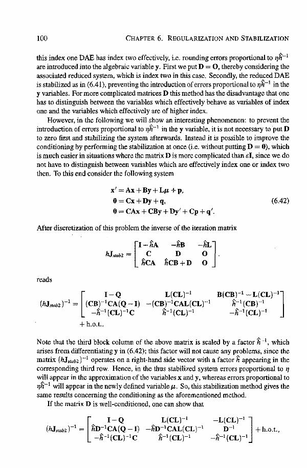
100 CHAPTER 6. REGULARIZATION AND STABILIZATION

tbis index one DAB bas index two effectively, i.e. rounding errors proportional to 1jh-1

are introduced into tbe algebraic variabie y. First we put D = 0, tbereby consictering tbe associated reduced system, which is index two in tbis case. Secondly, tbe reduced DAB is stabilized as in ( 6.41 ), preventing tbe introduetion of errors proportional to f'/h-1 in tbe y variables. For more complicated matrices D tbis metbod bas tbe disadvantage tbat one bas to distinguish between tbe variables which effectively behave as variables of index one and tbe variables which effectively are of higher index.

However, in tbe following we will show an interesting phenomenon: to prevent tbe introduetion of errors proportional to f'/h-1 in the y variable, it is not necessary to put D to zero first and stahilizing tbe system afterwards. Instead it is possible to improve tbe conditioning by performing the stabilization at once (i.e. without putting D 0), which is much easier in situations where tbe matrixDis more complicated than el, since we do nothave to distinguish between variables which are effectively index one or index two tben. To tbis end consicter tbe following system

x' = Ax + By +LIJ. + p,

0 Cx+Dy+q,

0 CAx+CBy+Dy' +Cp+q'.

Mter discretization of tbis problem tbe inverse of tbe iteration matrix

[

I-hA -hB hJstab2 = C D

hCA hCB+D

-hL] 0 . 0

reacts

(hlstabz)-1 = [(CB)-~CA~Q I) -fi-1 (CL)-1C

+h.o.t ..

L(CL)-1

-{CB)-1CAL(CL)-1

fi,-t(CL)-1

(6.42)

Note tbat the tbird block column of tbe above matrix is scaled by a factor fi-1, which arises from differentiating yin (6.42); this factor will not cause any problems, since tbe matrix (hlstabz)-1 operates on a right-hand side vector witb a factor h appearing in tbe corresponding third row. Hence, in tbe tbus stabilized system errors proportional to rJ will appear in tbe approximation of tbe variables x and y, whereas errors proportional to rJh-1 will appear in tbe newly defined variabie IJ.. So, tbis stabilization metbod gives tbe same results concerning tbe conditioning as tbe aforementioned metbod.

If tbe matrixDis well-conditioned, one can showtbat

-L(CL)-1]

o-l + h.o.t., -fi-1(CL)-1

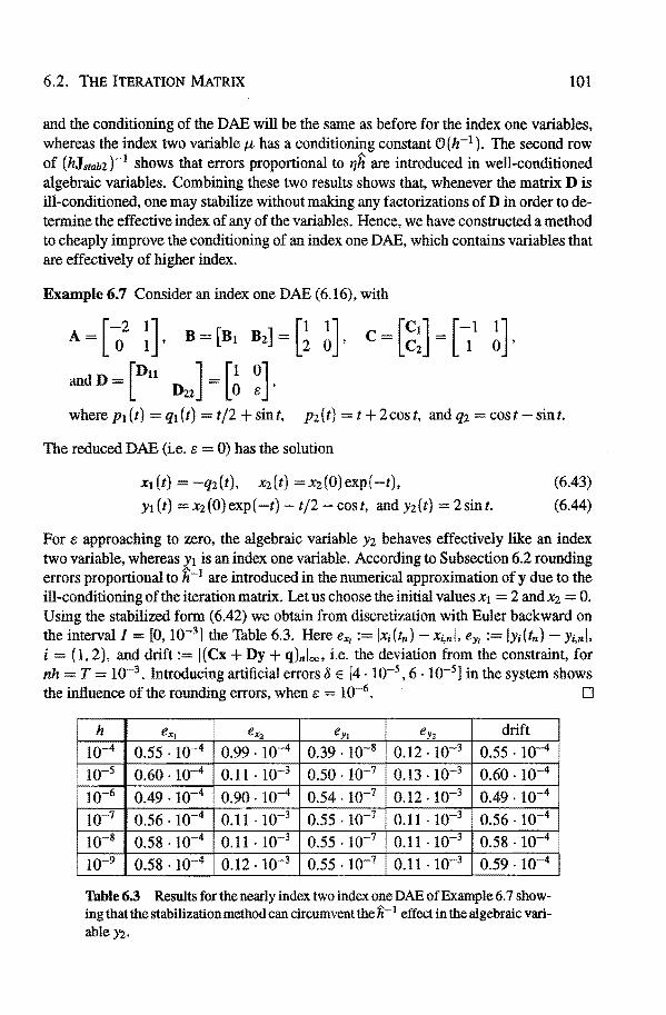
6.2. THE ITERATION MATRIX 101

and the conditioning of the OAE will be the same as before for the index one variables, whereas the index two variabie f1, has a conditioning constant CJ(h-1 ). The second row of (hJstabz)-1 shows that errors proportional to l'}h are introduced in well-conditioned algebraic variables. Combining these two results shows that, whenever the matrix D is ill-conditioned, one may stabilîze without rnaicing any factorizations of D in order to de­termine the effective index of any of the variables. Hence, we have constructed a method to cheaply improve the conditioning of an index one OAE, which contains variables that are effectively of higher index.

Example 6.7 Consider an index one OAE (6.16), with

A=[~2 ~l B=[B1 Bz]=G ~]. C=[~:]=[~l ~]. and D = [Dn Dzz] = [~ ~l where p1 (t) = q1 (t) = t/2 +sint, pz(t} = t + 2cos t, and qz =cos t- sint.

The reduced OAE (i.e. 8 = 0) has the solution

xt(t) = -qz(t), xz(t) =xz(O)exp(-t), (6.43)

Y1(t) =xz(O)exp(-t)-t/2-cost, andyz(t) =2sint. (6.44)

For 8 approaching to zero, the algebraic variabie y2 behaves effectively like an index two variable, whereas y1 is an index one variable. According to Subsection 6.2 rounding errors proportional to h.-1 are introduced in the numerical approximation of y due to the ill-conditioning of the iteration matrix. Let us choose the initia! values x1 = 2 and x2 = 0. Using the stabilîzed form (6.42) we obtain from discretization with Euler backwardon the interval!= [0, 10-3] the Table 6.3. Here exi := lx;(tn) -x;,nl. eyi := iy;(tn)- Y;,nl. i= (1, 2), and drift:= I(Cx +Dy+ q)nlcx:.. i.e. the deviation from the constraint, for nh = T = 10-3 • lntroducing artificial errors 8 E [4 · 10-5 ,6 · 10-5] in the system shows the influence of the rounding errors, when 8 = 1 o-6. 0

h ex, ex2 ey, eY2 drift 10-4 0.55.10-4 o.99 .10-4 0.39 .10-8 0.12 ·10-3 o.55 .10-4

• 10-s o.6o .10-4 0.11 .lQ-3 I o.5o .10-7 o.I3 .10-3 o.6o .10-4

10-6 0.49 ·10-4 o.9o .10-4 o.54 .10-7 0.12. 10-3 o.49. 10-4

10-7 o.56 ·10-4 0.11 .lQ-3 0.55 ·10-7 0.11 . 10-3 o.56. 10-4

10-s o.58 ·10-4 0.11. 10-3 o.55. 10-7 0.11 . 10 3 0.58 ·10-4 10-9 0.58 ·10-4 0.12. 10-3 o.55 .w-7 0.11 .lQ-3 0.59. w-4

Table 6.3 Results for the nearly index two index one DAE ofExample 6.7 show­ing that the stabilizationmethod can circumvent the 'h-1 effect in the algebraic vari­abie Yz.

102 CHAPTER 6. REGULARIZATION AND STABILIZATION

6.3 ERROR ESTIMATION FOR STEP-SIZE CONTROL AND TERMINATION OF NEWTON ITERATIONS

This section explains how the step-size control of BDF codes, and in particular DASSL (cf. [66]), works. In Subsection 6.2.1 we have shown that the iteration matrix used by e.g. BDF is poorly conditioned when the step-sizeis small. We will show that this may cause various complications in the numerical solution by ( variabie step-size) BDF codes when solving DAEs of higher index. These problems can be circumvented by sealing the error estimates, i.e. both the estimates for the local error and the estimates for terminating the Newton iterations.

Here, we concentrate on the general (nonlinear) implicitform of a DAE, motivated by the fact that we use a code, i.e. DASSL ( cf. [ 66]), which requires the system of equations in this impHeit form. In order to understand these problems we first investigate the error equation for the numerical solution by a BDF code of the DAE (3.1 ). Application of a k-step BDF metbod leads to the following difference equation

(6.45)

where, as introduced inSection 3.2, p,. is the generating polynomial of the variabie step­size BDF method, i.e. p,. (z) := I:Lo ai, nt-i. Let x,. be the exact salution of this differ­ence equation. The previous equation is solved by Newton iteration. This results in the numerical solutionx,. of (6.45), which introduces an errorE,. :=in- Xn due to termillat­ing the Newton iterations early. Let en:= x,.- x(t,.) be the global error. Then we get

o f(t,.,x,.,h;;-1 Pn(E)x"_k)

f(t,., x,.+ E,., h;;-1 p,.(E)(Xn-k +En-k))

f(t,.,x(t,.) +en +E,., h;1 p,.(E)(x(t"_lc) +en-k +En-k)).

The local truncation error -r,., say, is defined by -r,. := p,. ( E)x( tn-k) - h,.x' ( t,.). We find

0 = f(t,.,x(t,.) +en +E,.,x'(t,.) + h;1-r,. + h;1 Pn(E)(e"_k +En-k)).

Using Taylor expansions around x(t,.), x'(t,.} we find the linearization (cf. (4.la))

0 ~ Á,.(h;1-r,. + h;;-1 Pn (E)(e,._k +En-k)) + B,.(e,. + E,.), (6.46)

where Á,. and B,. are defined by

Á,.:= :,(t,.,x(t,.),x'(t,.)) and B,.:= :(t,.,x(t,.),x'(t,.)),

respectively. We thus find

(6.47)

6.3. ERROR ESTIMATION 103

where hn := hnfao,n (since {Jo= 1) as in Subsection 6.2.1. In Subsection 6.2.1 we have shown that the iteration matrix hJ is poorly conditioned for DAEs of higher index. Note that the scaled matrix [1 tî-1 1] hJ is equal to the matrix Än + hnBn. Together with the error equation (6.47) this implies that some of the variables can have large errors, since they are amplified by positive powersof 1i;;1. This will cause failure of the error esti­mating process both with respect to the step-size control and with respect to terrninating the Newton iterations; this then will result in inefficient behaviour or even failure of the code. To understand these effects we will examine the relation between the local error and the truncation error. In first order terms this relationship is given by

1- .,.,._ 1-ên ='= -aO,n (An + hnBn)- Ant'n.

From equation (6.20) we can obtain the following estimate for ên as a function of t'n in the index one case

_ . [C>(l) C>(l) ] [I 0] en= C>(l) C>(fi;;t) 0 0 Tn [

C>(l) 0] C>(l) 0 Tn,

hence the truncation error Tn is not amplified. Now, the step-size must be chosen such that the estimation ESTn of the local error ên is less than a given tolerance. lt is clear that for the index one DAE the same error estimation as for ODEs can be used, since for ODEs we use the relation e ~ t' = e>(fik+t ). However, forsemi-explicit index two systems (6.24) we find with the help of (6.22) that

_ . [ C>(l) C>(h;;1 )] [I 0] [ C>(l) 0]

en= C>(fi;;t) C>(fi;;2) 0 0 t'n = C>(fi;;t) O Tn, (6.48)

which implies that in this case the truncation error Tn is amplified by fi;; 1 and that the local error will not be of order C>(jÇ+1 ) as expected by the code. In order to use a criterion for step-size control, we use the scaled error estimate

ESTn · [~ t] en,

which is C) (fi!+ 1 ) as the code expects. Care has to betaken to ensure that the scaled error estimate ESTnis of order of the toleranee TOL. Hence, we allow the largest errors in the variables of index two which is more or less satisfactory since in general these are the ill-posed variables. Index three Hessenberg systems (6.29) yield

This implies that we should use the scaled error estimate

104 CHAPTER 6. REGULARIZATION AND STABILIZATION

in order to get ESTn ~ TOL. Here, again the larger errors are allowed in variables of higher index. For equations of motion for mechanica! systems, this means that the posi­tion variables are controlled to order hk+1 while the veloeities and the Lagrange multi­pliers are controlled to order hk and 'hk-l, respectively.

The global error en and the error En, due to terminating the Newton iterations after a finite numer of steps, are approximately related by the following recurrence relation

This shows that the local error is influenced not only by the error En at time tn, but also by the errors En-1 , • • • , En-k made at previous times. This gives the following relationship between the local error ê and the error E

k

ên = -En ao,n (Än + hnBn)-1 Än L a;,nEn-i· (6.49) i=l

Hence, ê and E are related by the matrix factor (Än + hnBn)-1 Än. Again, this means that some components of E are amplified by positive powers of Îi;;1

• Therefore, some vari­ables have to be solved more precisely than others to limit the influence of the algebraic errors on the local error in order to let the local error ê be of the order of the toleranee (i.e. ê ~ C>(TOL )). We can see from (6.49) that the amplification of the i-th component of Eis found by consictering the maximum power ofÎi;;1 in the i-th column of (Än + hnÛn)-1 Än. To this end we have to scale the estimates for terminating the Newton iteration in such a way that the scaled error estimates are of the order of the tolerance. Consicter for example thesemi-explicit index two DAE (6.24). From (6.48) we can see that the x-components of E (say Ex) are not amplified at all, whereas the y-components of E (i.e. Ey) are amplified by ii;;1 . In order to let the local error ê be of the order of the toleranee we must require for the estimates of the local error that ES~ ~ TOL and hnEST! ~ TOL. Hence, the sealing vector is [1, hnF· For the Hessenberg index three system (6.29) we see that Ex is amplified by Îi;;1 and Ey is amplified by Îi;;2 , whereas Ez is not amplified at all. This implies that we must choose the sealing vector [Îln, ti;;, l]T to obtain ê = ö(TOL).

In the foregoing analysis we have studied the propagation of errors both caused by the truncation error and caused by terminating the Newton iterations early. We showed that for DAEs of higher index some componentsof the errors may be amplified by powersof Îl;;1, which leads to severe complications for the step-size control and the termination of the iterations. This may result in failure of DAE codes designed for DAEs of index one (e.g. DASSL). However, with the suggested modifications the usual errorestimates can be applied. That means that DAEs of higher index can be solved by DAE codes designed for DAEs of lower index. Indeed, solving higher index DAEs with the modified code is camparabie to solving index one DAEs (see [8]). A disadvantage of this metbod is that now some variables are controlled less accurately, which suggests that those variables may exhibit larger errors than expected.

6.4. APPLICATION TO MULTIBODY SYSTEMS 105

6.4 APPLICATION TO MULTIBODY SYSTEMS

With the modifications of the previous section we can use the BDF code DASSL to solve DAEs of higher index efficiently. Therefore, we can solve the equations of motion for mul ti body systems in index three form (3.19). However, since the velocity variables are scaled by 'h and the algebraic variables are scaled by fi2 the solution of the index three DAE can exhibit large errors. Therefore, we rednee the index and use the projection metbod (6.12) in order to alleviate drift. Now, only >.. bas to be scaled by 'h. In the fol­lowing example we compare both methods for the crank -slider mechanism shown in Pi g­ure 1.5 (see also Example 2.6).

Example 6.8 Let the lenghts of the rods belt = 1, h = 2 and the mass be m 1 = 1, m2 = 2. With initial valnes (/Jt (O) = 0.5236 and 4J1 (O) = 0, we find the solution as plotted in Figure 6.4 for 0 :$ t :$ 10. The plot of the y coordinates of the bodies B1 and B2

shows that y1 = Y2· which is caused by constraining the distal end of rod B2 to move along the x-axis. In Table 6.4 we compare the numerical solution of the index three DAE

x

OL-------~------~ 0 5 10

-t

-t

-0.5 0

\J \.

f\ {\ {\ {\

t \. \. 5 10 -t

Figure 6.4 Solution for the crank-slider mechanism for TOL = 1 o-6 • The solid lines represent the generalized coordinates of body B1• The generalized coordi­nates of body B2 are represented by the dotted lines.

and the projection method. The error e, say, at the endpoint of the integration interval in the numerical solution of the DAE (3.1) is the weighted root mean square norm (cf. [9])

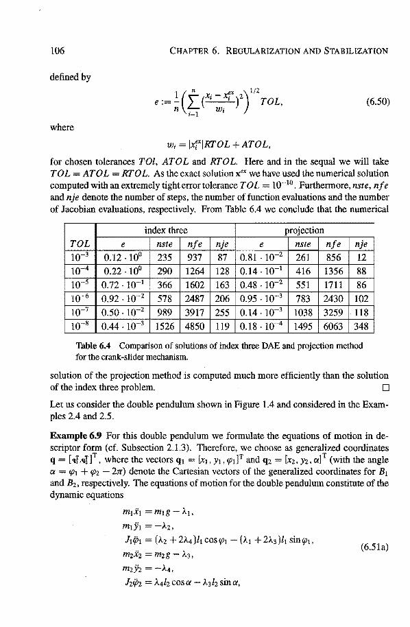
106 CHAPTER 6. REGULARIZATION AND STABILIZATION

defined by

(6.50)

where

Wi = lx;xiRTOL +ATOL,

for chosen tolerances TOl, ATOL and RTOL. Here and in the sequal we will take T 0 L = AT 0 L = RT 0 L. As the exact salution xex we have used the numerical salution computed with an extremely tighterrortolerance TOL= w-to. Furthermore, nste, nfe and nje denote the number of steps, the number of function evaluations and the number of Jacobian evaluations, respectively. From Table 6.4 we conetude that the numerical

index three projection

TOL e nste nfe nje e nste. nfe nje w-3 0.12. 10° 235 937 87 o.8t . w-2 261 856 12 10-'4 0.22 ·10° 290 1264 128 0.14·10-1 416 1356 88 w-s o.n .w-1 366 1602 163 0.48. w-2 551 1711 86 w-6 o.92 .w-2 578 2487 206 o.95. w-3 783 2430 102 w-1 o.5o .w-z 989 3917 255 0.14. w-3 1038 3259 118 w-s 0.44 .w-3 1526 4850 119 0.18. w-4 1495 6063 348

Thble 6.4 Comparison of solutions of index three DAE and projection method for the crank-slider mechanism.

salution of the projection metbod is computed much more efficiently than the solution of the index three problem. D

Let us consider the double penduturn shown in Figure 1.4 and considered in the Exam­ples 2.4 and 2.5.

Example 6.9 For this double penduturn we formulate the equations of motion in de­scriptor form (cf. Subsection 2.1.3). Therefore, we choose as generalized coordinates q = [<~I ,qJ] T, where the veetors q1 [xt, Yt , CfJt ]T and q2 [xz, yz, a] T ( with the angle a = CfJt + cpz - 2n') denote the Cartesian veetors of the generalized coordinates for B1

and B2, respectively. The equations of motion for the double pendulum constitute of the dynamic equations

mt.Xt mtg- Ät,

mt.Yt ->..2,

lti/Jt (J..2+2>..4)ltCOSC(Jt-(Ä1 +2J..3)ltsincpt,

m2xz = m2g- À3,

m2.Yz = ->..4,

l2i/Jz = Ä4[z cos a - Ä3[z sin a,

(6.5la)

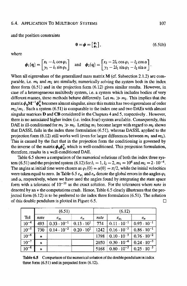
6.4. APPLICATION TO MULTIBODY SYSTEMS 107

and the position constraints

0=4>=[~]. (6.51b)

where

Wh en all eigenvalnes of the generalized mass matrix M ( cf. Subsection 2.1.2) are com­parable, i.e. m1 and m2 are similarly, numerically solving the system both in the index three form (6.51) and in the projection form (6.12) gives similar results. However, in case of a heterogeneaus multibody system, i.e. a system which includes bodies of very different masses, these methods behave differently. Let m1 » m2• This implies that the matrix (j}qM-14>! becomes almost singular, since this matrix bas two eigenvalnes of order m2 fm1 • Such a system (6.51) is camparabie to the index one and two DAEs withalmost singular matrices D and CB considered in the Chapters 4 and 5, respectively. However, there is no associated higher index (i.e. index four) system available. Consequently, this DAE is ill-conditioned for mt » m2• Letting mt become larger with regard to m2 shows that DASSL fails in the index three formulation (6.51), whereas DASSL applied to the projection form (6.12) still works well (even for larger differences between m1 and m2 ).

This is caused by the fact that in the projection form the conditioning is govemed by the inverse of the matrix 4>114>!, which is well-conditioned. This projection formulation, therefore, results in a well-conditioned DAE.

Table 6.5 shows a comparison of the numerical solutions of both the index three sys­tem (6.51) and the projected system (6.12) for h = 1, lz = 2, m1 = 106 and m2 = 2 · w-4

•

The angles at initial time were chosen as cp1 (O) = a(O) = rr/2, while the initial veloeities were taken equal to zero. In Table 6.5 erp1 and ea denote the global errors in the angles cp1

and a, respectively, where we have used the angles found by integrating the state space form with a toleranee of w-to as the exact solution. For the tolerances where nste is denoted by an * the computations crash. Hence, Table 6.5 clearly illustrates that the pro­jected form (6.12) is to be preferred to the index three formulation (6.51). The salution of this double pendulum is plotted in Figure 6.5. D

(6.51) (6.12)

Tol nste e'Pt ea nste e'Pt ea w-4 493 0.33. w-1 0.13. 101 774 o.n .w-1 o.93 .w-1 w-s 730 o.t4. w-2 0.20. 101 1242 0.16 ·10-3 o.86 .w-1 w-6 * 1798 0.10. w-3 0.76 .w-2

w-1 * 2050 0.30 ·10 6 0.24 .w-3

w-s * 5168 o.8o .w-5 o.2s .w-5

Table 6.5 Comparison ofthe numerical salution ofthe double pendulumin index three form (6.51) and in projected form (6.12).

108 CHAPTER 6. REGULARIZATION AND STABILIZATION

(/Jl

1 1

-1

2 3 4 5 6 7 8 9 10 -t

a 1

1-: -2

-3

-40 3 4 5 7 8 9 10 -t

Figure 6.5 Solution for the double pendulum for T 0 L = 10-6 .

Hence, solving tbe equations of motion for mul ti body systems in tbe projection farmu­lation (6.12) witb tbe BDF code DASSL using tbe appropriate modifications (see Sub­section 6.3) results in an efficient an robust metbod for simulating multibody dynamics. The use of tbe aforementioned projection form results in a larger system tban tbe original index tbree form. One may conclude tbat as a result, tbe linear algebra might be much more expensive tban in tbe original form. Fortunately, tbe efficiency of tbe metbod can be improved further by reducing tbe amount of workin tbe linear algebra as suggested in [34, 43]. Each step of a BDF metbod requires tbe salution oflinear systems ( cf. ( 6.46)) oftbeform

[

-fi-t I I 0 4»!] [8q] [a] 0 -fi-1M 4»! 0 &v = b t/Jq 0 0 0 8). . c ' 0 t/Jq 0 0 8JJ, d

(6.52)

found by supplying an analytica! Jacobian, neglecting the derivatives of M, f and tPq· Solving (6.52) is equivalent to solving two smaller linear systems, viz.

(6.53)

lmplementing tbis may lead to a considerable reduction in computing time (in [ 43] a factor tbree is reported forsome problems).

7 DISCONTINUITIES IN

MECHANICAL SYSTEMS

Many systems in simulation and control give rise to systems of differentlal algebraic equations (DAEs) with forcing functions containing discontinuities in the form of finite jumps either in components of the forcing functions themselves or in some derivatives of them. Quite often multibody systems exist in an environment where impulsive forces are exerted on the system. Those impulsive forces are defined as large forces exerted for a short time interval. Examples of systems experiencing impulsive forces are models of crash-victims duringa crash, machine couplers and robot grippers. Force discontinuities also occur in conversion from slip to stick conditions and vice versa, which can happen in the presence of Coulomb friction. Other kinds of singularities that often occur for roe­ehanical systems are e.g. contact phenomena, hysteresis and functions supplied by data bases.

The lack of smoothness causes numerical difficulties, since the convergence theory of discretization schemes as well as the step-size and order control usually require differ­entiability up to some given order. As a consequence, the step-size selection may break down and there is no safe local error estimation anymore. Therefore, a numerical integra­tor will behave very inefficiently in the presence of a singularity.

In the following, the occurring difficulties are explained and demonstraled by numer­ical examples. A metbod is developed to handle the discontinuities in an efficient and robustway.

7.1 NUMERICAL PROBLEMS DUE TO SHOCKS AND DISCONTINUITIES

In many applications, the appearance of discontinuities can be modelled by the use of switchingfunctions, resulting in discontinuons differential algebraic equations of the fol-

110 CHAPTBR 7. DISCONTINUITIBS IN MBCHANICAL SYSTBMS

lowingform

x {ft(t,x,y), f2(t, x, y),

0 = g(t, X, y).

where s is the switching function.

if s(t, x) > 0,

if s(t, x) < 0, (?.la)

(7.lb)

Using these switching functions the singularity is localized at the root of s. We shall call the surfaceS := {(t, x)l s(t, x) = 0} the manifold of discontinuity. Furthermore, we define the regions s+ := {(t, x)l s(t, x) > 0} and s- := {(t, x)l s(t, x) < 0}. Inside these regions s+ and s- the dynamic equation (?.la) is characterized by the forcing functions f1 and fz, respectively. In either region, the problem {7 .1) can be solved by classica! meth­ods.

A discontinuous differentlal equation can be integrated numerically in various ways. A first metbod is to use a variabie step, variabie order integration metbod with local error control, thereby hoping that the step-size mechanism will handle the discontinuity ap­propriately. In [36] and [ 42] examples are given, which show how multistep and Runge­Kutta methods deal with such a singularity. Both methods detect the discontinuity fairly well, al heit by means of numerous rejected steps, since the presence of a discontinuity is usually noticed by a very large value of the local error estimate; the latter fact results in rejecting the step and a dramatic reduction of the step-size and possibly of the order of the method. Back again in the smooth region the step-size will usually be increased until the code tries to step over the singularity again. Then the sameprocedure is repeated and the code will pass the singularity only after several repetitions of this procedure. So, in general many steps may be rejected when passing such a discontinuity, yielding a very inefficient method. This is illustrated by the following

Example 7.1 Consider the ODE

. {0, t::: 10, x=

5, t > 10, x(O) = 10. (7.2)

Figure 7.1 shows the inefficient behaviour of a BDF code (with TOL= 10-4) when ig­

noring the discontinuity. D

However, it might even be possible that the integrator misses the discontinuity completely. Consider e.g. the following

Example7.2

{

5, t::: 10,

i 10, 10 < t < 11,

5, t '2: 11,

x(O) = 0. (7.3)

7 .2. TREATMENT OF DISCONTINUITIES

15

10

2 4 6 8 10 12 14 16 18 20

-t Figure 7.1 Behaviour of a BDF code ignoring the discontlnuity of system (7.2). Successful steps are marked with a o, while rejected steps are marked with an *·

111

BDF fails for this rather simple system because it steps over the discontinuity and will follow the solution branch x = 5t. This effect is due to so-called superstability of BDF (cf. [55, 60]) and it will occur for all tolerances. 0

So, standard codes for the numerical solution of ODEs handle, if at all, discontin ui ties in­efficiently. Therefore, integration codes have been modified to detect singularities more precisely and to handlethem more appropriately. These singularity detecting codes have been developed for both multistep methods ( cf. [36]) and Run ge~ Kuttamethods ( cf. [24]). They are based on estimates of the order and magnitude of the discontinuity and hence the step-size which keeps the error under control when passing a discontinuity.

Despite the efforts spent to construct such singularity detecting codes, the best avail­able methods to handle the appearance of discontinuities are methods which use switch­ing functions to explicitly indicate the appearance of a discontinuity. These methods stop the integration at the surface of the discontinuity and restart the computation with the new right-hand side. These methods appear to be not only more efficient but also more accurate in integrating discontinuous problems.

7.2 TREATMENT OF DISCONTINUITIES

In the previous Chapter 6 we have shown that the problem (7 .1) can be solved by classica! methods in either of the regions s- and s+. Problems occur when the switching function

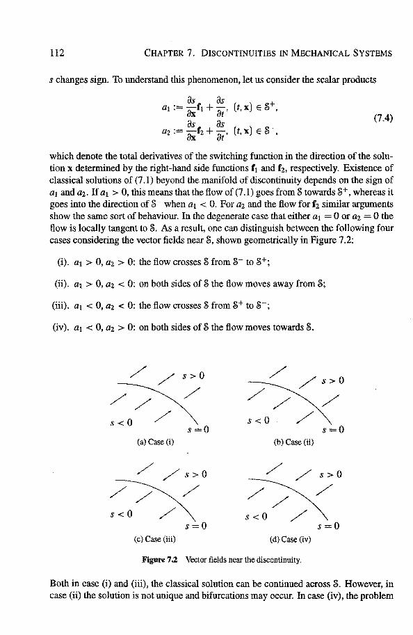
112 CHAPTER 7. DISCONTINUITIES IN MECHANICAL SYSTEMS

s changes sign. To understand this phenomenon, let us consider the scalar products

.as as + a1 .= (Jxf1 + fJt' (t,x) ES ,

as as az := (Jxf2 +at' (t,X) Es-,

(7.4)

which denote the total derivatives of the switching function in the direction of the solu­tion x determined by the right-hand side functions f1 and f2, respectively. Existence of classica! solutions of (7 .1) beyond the manifold of discontinuity depends on the sign of a1 and a2• If at > 0, this means that the flow of (7.1) goes from S towards s+, whereas it goes into the direction of s- when at < 0. For a2 and the flow for f2 similar arguments show the same sort of behaviour. In the degenerate case that either a1 0 or az 0 the flow is locally tangent to S. As a result, one can distinguish between the following four cases consirlering the vector fields near S, shown geometrically in Figure 7.2:

(i). al > 0, az > 0: the flow crosses s from s- to s+;

(ü). a1 > 0, az < 0: on both sides of S the flow moves away from S;

(iii). al < 0, az < 0: the flow crosses s from s+ to s-;

(iv). a1 < 0, a2 > 0: on both sides of S the flow moves towards S.

//

// s<O /

(a) Case (i)

s>O

/

s=O

/

// s<O /

(b) Case (ii) s=O

/ /s>O

// /

/ / s>O

s<O /

/ // / s<O

s=O s=O (c) Case (iii) (d) Case (iv)

Figure 7.2 Vector fields near the discontinuity.

Both in case (i) and (iü), the classical salution can be continued across S. However, in case (ii) the solution is not unique and bifurcations may occur. In case (iv ), the problem

7 .3. ÛCCURRENCE OF DISCONTINUITIES IN MULTIBODY DYNAMICS 113

has no langer a classica! salution since the salution is trapped in the discontinuity man­ifold S. However, one can show that the system has a generalized salution (cf. [25]), then, which says that the generalized salution has its derivative in the convex hull of ft and fz, i.e.

x = vft + ( 1 - v )fz, with 0 ~ v ~ 1.

The value v acts as a control variabie which forces the solutions to stay in the manifold S (as proposed in [19] and [77]), implying that the salution has to satisfy the DAE

x= vft + (1- v)fz =: f(t,x, y, v),

0 = g(t, x, y),

0 s(t, x).

It is obvious that the control variabie v is an index two variable, since

as aë --=at az =f:-0. axav

(7.5a)

(7.5b)

(7.5c)

This implies that one can solve for v from (7.5a) and (7.5c), indeed, taking the total derivative of (7.5c) and substituting (7.5a) yields

implying that

sx(vft+(l v)fz)+sr=O,

V= St +sxfz

Sxfl -sxfz

Substitution of this value of v into (7 .Sa) results in the DAE

. az a1 x= ft+ fz,

az-at a1 -az 0 = g(t, X, y).

(7.6)

(7.7a)

(7.7b)

Hence, the salution in the manifold S is described by the vector field which satisfies the DAE (7 .7). The salution of the discontinuous DAE (7 .1) willleave the discontinuity manifold S when v = 0 or v 1, meaning that one of the scalars a1 or a2 changes sign.

7.3 OCCURRENCE OF DISCONTINlTITIES IN MULTffiODY DYNAMICS

In Section 7.1 we have explained the numerical probieros in dealing with discontinuities. Treatment of these shocks by using switching functions means that all possible switching functions must be provided by the user, it is convenient to have at one's disposal some sort of library with possible switching functions and methods to deal with them. Por that reason, it is important to recognize the various kinds of discontinuities which may occur when modelling mechanica! systems. The possibly appearing discontinuities can be subdivided into several classes, e.g.

114 CHAPTER 7. DISCONTINUITIES IN MECHANICAL SYSTEMS

(i). impacts. These impacts arise naturally in the crash-safety field, where one stud­ies the response of multibody systems during crashes. They are characterized by instantaneous appearing (and possibly very large) forces. These forces cause dis­continuitles in the velocities, since the movement of the mechanica! system may be stopped abruptly.

Example 7.3 Consider for example a pendulum moving under the influence of gravity, cf. Example 2.1. Mter some time this pendulum hitsawall ( cf. Figure 7 .3). On impact the velocity of the pendulum will almost immediately drop to zero due to a suddenly increasing elasto-plastic force as a function of the penetration into the wall. The example will be worked out in Example 7.9 and numerical results shown in Figure 7.7. 0

Figure 7.3 Impact of pendulum into a wall.

(ü). Contact problems for rigid bodies give rise to algebraic equations as the touching of bodies leads to algebraic constraints in a natura! way.

(iii). Coulomb friction. When one solid body slides over another or over a surface, dry friction or Coulomb friction is generated. Like other frictional forces, this force is dissipative and nonlinear.

Example 7.4 Consicter asolid block sliding with a velocity q relative toa rough solid plane (cf. [19, 39]). The force of the plane acting on the block consists of

Ft

---lf JtiNI

-JtiNit---

Figure 7A Coulomb friction.

7 .4. U SAGE OF THE SWITCHING FUNCTIONS 115

the normal force N perpendicular to the surface and the Coulomb friction force F f parallel to the surface and opposing the motion. The classicallaw of sliding friction states that this force can be expressed as

(7.8)

where e is the unit vector tangentlal to the surface. The Coulomb friction coef­ficient f), depends on the roughness of the surfaces and the matenals used. The component in the positive e-direction of the friction force, i.e. Fr = e1F f, is plotted against the velocity in Figure 7.4 for the case of a constant normal force. In the so­called stick phase, i.e. when e1q = 0, the friction force is not uniquely determined. Then, the method, which has been explained inSection 7.2 (for at < 0, a2 > 0), may be applied, since IF rl :::: f,l,INI, always. D

(iv). Hysteresis describes the energy dissipation which can occurin mechanica! systems where several bodies can interact with each other, and in elasto-plastic materials. Hence, hysteresis is e.g. very important in the simulation of the interaction between the air bag and the steering wheel and in the rnadelling of seat beits. Consider the problem of Example 7.3 again:

Example 7.5 Due to the elasto-plastic force the pendulum will start moving into the opposite direction after some time. Because of energy dissipation the unload­ing elasto-plastic force will follow another curve than the loading force. This phe­nomenon is called hysteresis. D

(v). Input juncrions given in tabular form, to define e.g. material properties, accelera­tion fields, spring forces as a function of the relative elongation, and so on.

(vi). Breaking of interconnections between bodies. The removal of a joint can lead to a rapid movement of the remaining system and to a sudden increase of the constraint forcesin one or more of the remaining constraints (see [56]).

7.4 USAGE OF THE SWITCHING FUNCTIONS

The appearance of discontinuities is detected using switching functions as is already ex­plained in Section 7 .2. In this section we discuss the numerical simulation of systems ex­hibiting discontinuities. In Section 7.2 it was shown that a sign change of the switching function indicates the passing of a discontinuity. In order to simulate this phenomenon effectively one has to adjust the numerical integration metbod in order to incorporate the use of switching functions. This implies that the numerical integrator has to be extended with the following method, which follows from the analysis of Section 7.2 for treating discontinuous systems like (7.1) (cf. also [19, 42, 83]):

(i). LetXo be theinitial valueatinitial timeto. If s(t0 , xo) = 0 goto step (ii). Otherwise, if s(to, xo) =f 0 then solve the dynamic equation x ft tagether with the constraint

116 CHAPTER 7. DISCONTINUITIES IN MECHANICAL SYSTEMS

0 g (cf. (7.lb)) as long as (to, Xo) E 8+. However, when (to, Xo) E 8- onehas to solve tbe differential equation x fz together with tbe constraint equation (7 .1 b) until (t,x) E 8. When (t,x) E 8 goto step (ii).

(ii). Compute at and az as defined by (7.4).

(iii). If a1 > 0 and az > 0, then solve the DAB (7.1) witb x= ft(t, x) until (t,x) E 8. Go to step (ii).

(iv). If at < 0 and a2 < 0, tben solve tbe DAB (7.1) withx = f2 (t,x) until (t,x) e 8. Go to step (ii).

(v). If a1 < 0 and a2 > 0, tben tbe salution sticks in 8. Solve tbe index two DAB (7.5), until either a1 or a2 changes sign. Go to step (ii).

After tbe localization of a root, i.e. s(t*, x*) = 0, tbe forcing function is changed to tbe new mode and the discretization is adapted to tbe new situation. This means tbat the code should e.g. be restarted (for one-step metbods) ortbat tbe discretization order should be reduced. However, it appears tbat it is most effective to restart also in tbe case of mul­tistep metbods, since otberwise information of previous steps bas to be used. Unfortu­nately, tbis information doesnothave to be related in any way to the new situation which occurs after tbe discontinuity.

7.4.1 Root Finding

We have shown in Section 7.1 that it is important to find the location of tbe switch. The switch can e.g. be localized using an algoritbm for detecting a root of tbe switching func­tion, cf. DASSLRT (cf. [9]). In the sequel we proceed witb a switching funcion de­noted by a vector tunetion s. When a sign of any component of tbe switching function is changed, the code locates tbe root of s by a root search using an interval metbod lik:e tbe lllinois algorithm (cf. [17]). This metbod is a modification of thesecant metbod and gives cubic convergence witb tbree function evaluations. The root finding mechanism will be explained briefty.

After a successful step from tn to fn+ t. s( tn+l• Xn+ t) is evaluated. If s( tn, Xn) and s( tn+ 1. Xn+ 1) have a different sign in any of tbe components, a switch must have occurred in [tn, tn+l]. Then the root solver is used to find tbis switch, i.e. a root of f(z) in the in­terval [zo. z1] is sought, using secant-like iterations. Hence,

Z2 = Zl - /t (zt -Zo). ft- !o

(7.9)

After evaluating /(z2) the next secant step is performed until convergence. In case that fis a vector function, say f E !Rm, we want to find tbe leftmost root of fin [zo, z1]. There­

fore, we determine tbe maximum quotient ~~~~~/~o and then

f;t1UlX, 1 ( ) Z2 = Zt - Zl - Zo •

/;max,l - /;max,O (7.10)

7.4. USAGE OF THE SWITCHING FUNCTIONS 117

For the evaluation of s(t, x(t)) interpolation is used. Disadvantages of this metbod are:

(i). The root finder may fail due to ill-conditioned switching functions witb a large uncertainty domain.

(ii). The aforementioned metbod might experience problems with more-dimensional nonlinear switching functions

The following example illustrates tbe first problem.

Example 7.6 Consider the ODE

. {ft:= 3(t 3)2,

x= fz := sin(t 3),

subject to x(O) = -25. Clear1y the salution reads

x(t) {

2+(t 3) 3,

3 -cos(t 3).

2-x > 0,

2-x < 0,

2 -x> 0,

2-x < 0.

(7.11)

(7.12)

The switching function is given by s(x) = 2 -x and tbe switching parameters are given by a1 = -3(t 3)2 and a2 - sin(t- 3), respectively. In the exact solution the switch takes place at t 3 with x( 3) = 2. Starring in g+ the solution switches to g-. Ho wever, due to numerical errors the numerical switch may be situated to tbe left of t = 3. For t = 3 - 8 (0 < o « 1) tbe system is like tbe case a 1 < 0, a2 > 0; tbis results in a numer­ical solution which will stick on g during some time until the salution moves into g-. Table 7.1 shows some characteristics of tbe numerical solution when integrating from t = 0 to t = 4. The error e at t = 4 is defined bye:= lx(4) xnl. where Xn is tbe ap-

Tol #steps e w-2 45 0.13 -10-1

w-4 56 0.65 .w-1

Table 7.1 Comparison of BDF methods in order to show tbe effect of the use of switching functions.

proximation of x(4). For tolerances smaller tban 10-4 the numerical integration fails. D

So, a metbod based on rootfinding will fail when integrating discontinuous differentlal equations like the one shown in the aforementioned Example 7 .6. In the next section we will develop a more robust method, which is able to solve such equations as will be shown in Example 7 .8.

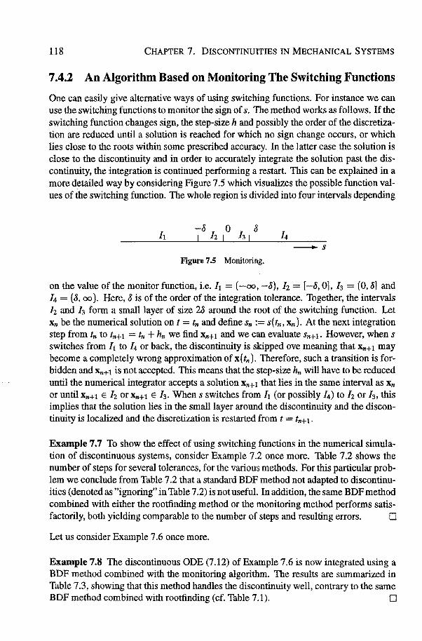
118 CHAPTER 7. DISCONTINUITIES IN MECHANICAL SYSTEMS

7 .4.2 An Algorithm Based on Monitoring The Switching Functions

One can easily give alternative ways of using switching functions. For instanee we can use the switching functions to monitor the sign of s. The method works as follows. If the switching function changes sign, the step-size h and possibly the order of the discretiza­tion are reduced until a solution is reached for which no sign change occurs, or which lies close to the roots within some prescribed accuracy. In the latter case the solution is close to the discontinuity and in order to accurately integrate the solution past the dis­continuity, the integration is continued performing a restart. This can be explained in a more detailed way by consirlering Figure 7.5 which visualizes the possible function val­ues of the switching function. The whole region is divided into four intervals depending

-8 0 8 I lz I h I

-s Figure 7.5 Monitoring.

on the value of the monitor function, i.e. ft = ( -oo, -8), [z = [-8, 0], h (0, 8] and !4 = ( 8, oo). Here, 8 is of the order of the integration tolerance. To gether, the intervals [z and 13 form a smalllayer of size 28 around the root of the switching function. Let Xn be the numerical solution on t = tn and define Sn := s(tn, Xn). At the next integration step from tn to tn+l = tn + hn we find Xn+l and we can evaluate Sn+!· However, when s switches from 1t to 14 or back, the discontinuity is skipped ove meaning that Xn+l may become a completely wrong approximation of x(tn). Therefore, such a transition is for­bidden and Xn+ 1 is not accepted. This means that the step-size hn will have to be reduced until the numerical integrator accepts a salution Xn+t that lies in the same interval as Xn

or until Xn+l E [z or Xn+1 E h When s switches from ft (or possibly 14) to [z or h this implies that the salution lies in the smalllayer around the discontinuity and the discon­tinuity is localized and the discretization is restarted from t = tn+l·

Example 7.7 To show the effect of using switching functions in the numerical simula­tion of discontinuous systems, consider Example 7.2 once more. Table 7.2 shows the number of steps for several tolerances, for the various methods. For this particular prob­lem we conclude from Table 7.2 that a standard BOF method not adapted to discontinu­ities ( denoted as "ignoring" in Table 7 .2) is not useful. In addition, the same BOF method combined with either the rootfinding methad or the monitoring method performs satis­factorily, both yielding comparable to the number of steps and resulting errors. 0

Let us consider Example 7.6 once more.

Example 7.8 The discontinuous ODE (7.12) of Example 7.6 is now integrated using a BOF method combined with the monitoring algorithm. The results are summarized in Table 7 .3, showing that this method handles the discontinuity well, contrary to the same BOF method combined with rootfinding (cf. Table 7.1). []

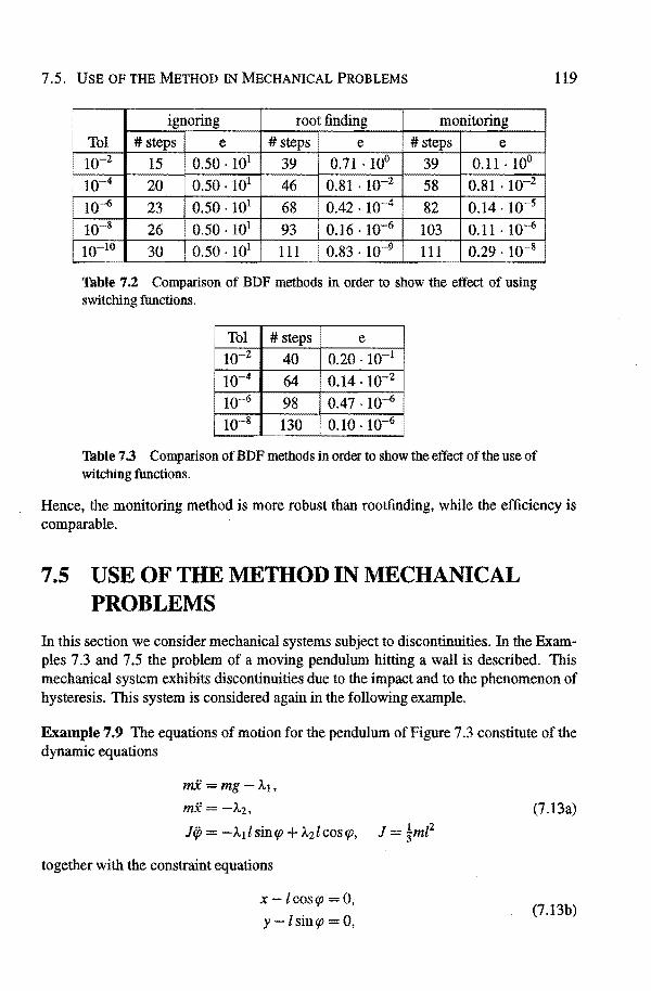
7.5. USE OF THE METHOD IN MECHANICAL PROBLEMS

ignoring root finding monitoring

Tol #steps e #steps~ e #steps e 10-2 15 0.50 ·101 39 0.71 . 10° 39 0.11 . 10° 10-4 20 0.50. 101 ~ 0.81·10-

2 58 o.81 . 10-2

10-6 23 0.50. 101 0.42. 10-4 82 o.14. 10-s 10-8 26 0.50. 101 0.16. 10-6 103 0.11 ·10-6

10-10 30 0.50 ·101 111 I 0.83.10-9 111 o.29 .10-8

Table 7.2 Comparison of BDF metbodsin order to show the effect of using switching functions.

Tol #st e 10-2 40 0.20.10-1

1o-4 64 o.14. 10-2

10-6 98 o.47 .10-6

10-8 130 0.10 ·10-6

Table 7.3 Comparison of BDF metbods in order to show tbe effect of tbe use of witching functions.

119

Hence, the monitoring method is more robust than rootfinding, while the efficiency is comparable.

7.5 USE OF THE METBOD IN MECHANICAL PROBLEMS

In this section we consider mechanica! systems subject to discontinuities. In the Exam­ples 7.3 and 7.5 the problem of a moving pendulum hitting a wall is descri bed. This mechanica! system exhibits discontinuities due to the impact and to the phenomenon of hysteresis. This system is considered again in the following example.

Example 7.9 The equations of motion for the pendulum of Figure 7.3 constitute of the dynamic equations

m.X=mg-J..1 ,

m.X = -J..2, (7.13a)

lip= -Àtlsintp + J..2lcostp, J = tmP

together with the constraint equations

x-lcostp =0,

y -l sintp = 0, (7.13b)

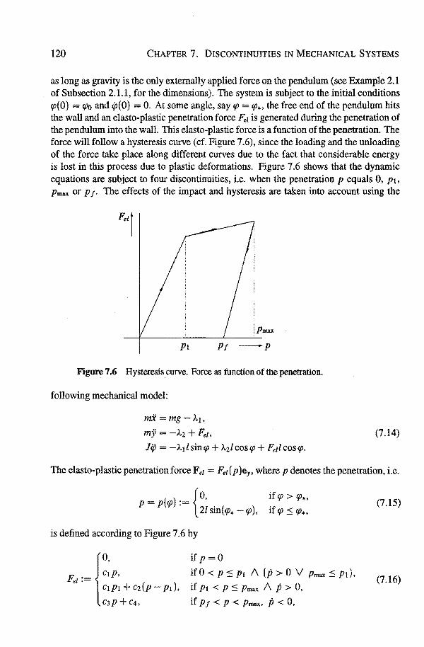
120 CHAPTER 7. DISCONTINUITIES IN MECHANICAL SYSTEMS

as long as gravity is the only extemally applied force on the pendulom (see Example 2.1 of Subsection 2.1.1, for the dimensions). The system is subject to the initial conditions q>(O) = q>o and q:>(O) = 0. At some angle, say q> = q>*, the free.end of the pendulom hits the wall and an elasto-plastic peneteation force Fe1 is generated during the penetration of the pendulom into the wall. This elasto-plastic force is a function of the peneteation. The force will follow a hysteresis curve (cf. Figure 7.6), since the loading and the unloading of the force take place along different curves due to the fact that considerable energy is lost in this process due to plastic deformations. Figure 7.6 shows that the dynamic equations are subject to four discontinuities, i.e. when the peneteation p equals 0, p1 ,

Pmax or p f. The effects of the impact and hysteresis are taken into account using the

:Pmax --4-------~-----L----~

Pt Pi -p

Figure 7.6 Hysteresis curve. Force as function of the penetration.

following mechanical model:

mX mg-}..1 ,

my = -Àz +Fel. Jip = -ltl sin<p + lzlcosq> +Fe~ I cosq>.

(7.14)

The elasto-plastic peneteation forceFel = Fel (p )e,, where p denotes the penetration, i.e.

p p(q>) := {0, 2l sin(q>*- q>),

if q> > q>*,

if q> ~ q>*,

is defined according to Figure 7.6 by

{

0,

F. Ctp, el:= CtPl + Cz(p

C3p+q,

ifp=O

if 0 < p ::S Pl A (p > 0 V Pmax ~ PI),

pi), if Pt < p ::S Pmax A p > 0,

if Pt < P < Pmax. P < 0,

(7.15)

(7.16)

7.5. USE OF THE METHOD IN MECHANICAL PROBLEMS 121

where for p ::: p 1 the unloading penetration force Fet becomes zero. The constauts c1 ,

cz and C3 are material constauts and C4 depends on the penetration Pmax· We find c4 from

C3Pmax + C4 = C3 {Pmax - P f) = CtPl + Cz (Pmax Pt ),

he nee

Let us choose l = 0.9, m = 30 and g = 9.81, and the initia! conditions cp(O) = 1.85 and ljJ(O) = 0. Fortheimpact we take cp* = 0. Moreover, the elasto-plastic force is defined by Ct = 8. 1Q5' Cz = 1 . 103 ' C3 = 2. 106 and Pt = 5 . 10-3 • In Figure 7.7 the numer­ical salution of this system is plotted, for the x-, as well as for the y-, the cp- and the ljJ-variable. It shows that on impact, i.e. at cp = cp*, the velocity of the pendulum drops almost at once to zero due to the increasing penetration force. Then cp reaches its mini­mum and the velocity ljJ even becomes slightly negative which means that the pendulum starts moving into the opposite direction under influence of this penetration force. How­ever, the penetration force is unloading and becomes equal to zero (cf. also Figure 7.6). This implies that the pendulum is going to oscillate until its motion damps out due to the loss of energy.

x y

t 0.5 I 0.5

0

0

0.5 1.5 2 0 0.5 1.5 2 -t -t

2 cp lP 0 r·: 1-1

-2 0.5

-3

0 -4

....0.5 -5 0 0.5 1.5 2 0 0.5 1.5 2

-t -t Figure7.7 Numerical solution of crashing pendulum computed with BDF code with T 0 L = 1 o-4 using the monitoring algoritbm.

D

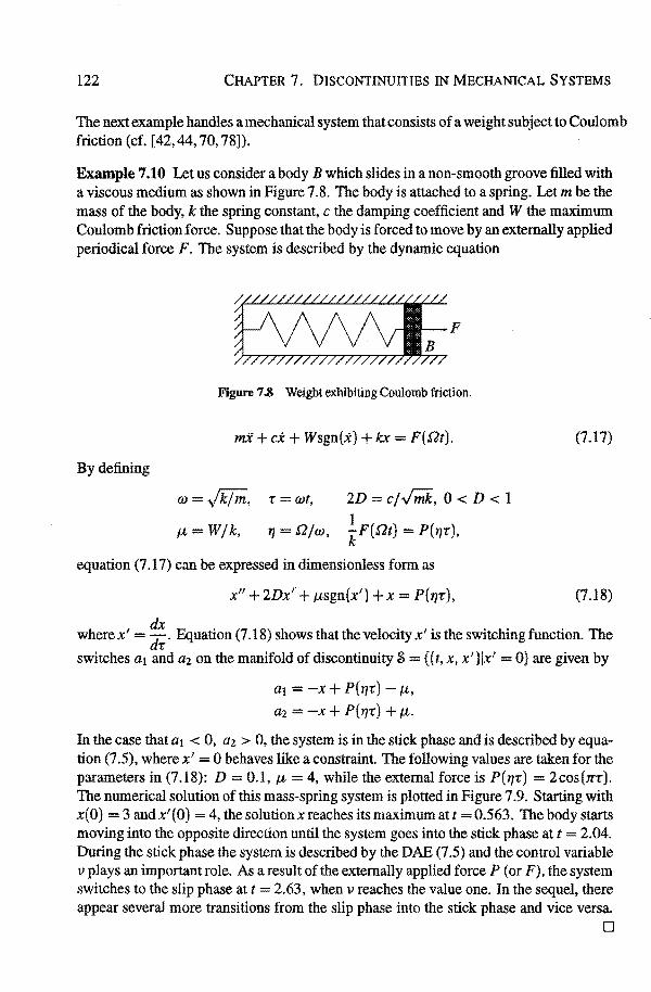
122 CHAPTER 7. DISCONTINUITIES IN MECHANICAL SYSTEMS

The next example handles a mechanica! system that consists of a weight subject to Coulomb friction (cf. [42,44, 70, 78]).

Example 7.10 Let us consider a body B which slides in a nort-smooth groove filled with a viseaus medium as shown in Figure 7 .8. The body is attached toa spring. Let m be the mass of the body, k the spring constant, c the damping coefficient and W the maximum Coulomb friction force. Suppose that the body is forced to move by an extemally applied periodical force F. The system is described by the dynamic equation

By defining

Figure 7.8 Weight exhibiting Coulomb friction.

m.X +ei+ Wsgn(i) + kx = F(ilt).

w=.[fim,

f..l=Wfk,

• = wt,

'1 ilfw,

2D = cj./mk, 0 < D < 1 1 kF(ilt) = P(t~<),

equation (7 .17) can be expressed in dimensionless form as

x"+ 2Dx,. + JLSgn(x') +x= P(t~<),

(7.17)

(7.18)

where x' = :. Equation (7 .18) shows that the velocity x' is the switching function. The

switches a1 and a2 on the manifold of discontinuity S = {(t, x, x')lx' = 0} are given by

a1 =-x+ P(t~•) - f..l,

a2 =-x+ P(t~•) + f..l. In the case that a1 < 0, a2 > 0, the system is in the stick phase and is described by equa­tion (7 .5), where x' = 0 behaves like a constraint. The following values are taken for the parameters in (7.18): D = 0.1, f..l = 4, while the extemal force is P(t~<) = 2cos(n-<). The numerical salution of this rnass-spring system is plotted in Figure 7.9. Starting with x(O) = 3 andx'(O) = 4, thesolutionxreaches itsmaximumatt =0.563. The body starts moving into the opposite direction until the system goes into the stick phase at t 2.04. During the stick phase the system is described by the DAE (7 .5) and the control variabie v plays an important role. As aresult of the extemally applied force P ( or F), the system switches totheslip phase at t 2.63, when v reaches the value one. In the sequel, there appear several more transitions from the slip phase into the stick phase and vice versa.

0

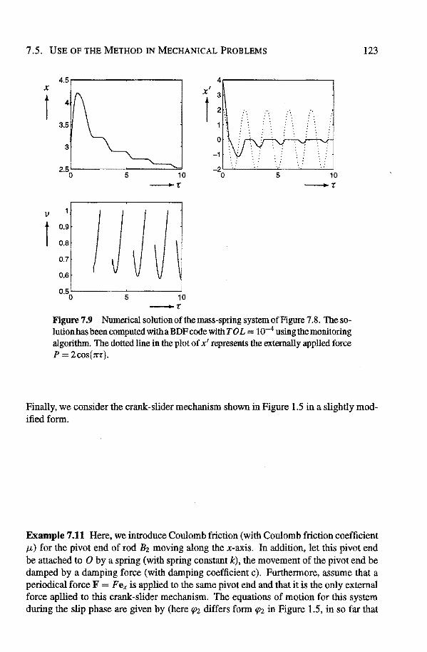
7.5. USE OF THE METHOD IN MECHANICAL PROBLEMS

x

t

V

t

4.5r----~------,

0.9

0.8

0.7

0.6

0.50 5

10

-r

10 -r

4

x' 3

t 2

1

0

-1

-2 0

: /\

: ·. ..

.. •.

: .. 5 10

-r

Figure 7.9 Numerical salution of the rnass-spring system ofFigure 7 .8. The so­lutionhas been computed witha BDF code with TOL = 10-4 using themonitoring algorithm. The dotted line in the plot of x' represents the externally applied force p 2 cos ( ïr't').

123

Finally, we consider the crank-slider mechanism shown in Figure 1.5 in a slightly mod­ified form.

Example 7.11 Here, we introduce Coulomb friction (with Coulomb friction coefficient f.L) for the pivot end of rod Bz rnaving along the x-axis. In addition, let this pivot end be attached to 0 by a spring (with spring constant k), the movement of the pivot end be damped by a damping force (with damping coefficient c). Furthermore, assume that a periodical force F Fex is applied to the samepivot end and that it is the only extemal force apllied to this crank-slider mechanism. The equations of motion for this system during the slip phase are given by (here qJ2 differs form (/J2 in Figure 1.5, in so far that

124 CHAPTER 7. DISCONTINUITIES IN MECHANICAL SYSTEMS

bere fJ2 is equal to q11 + fJ2 as chosen in Figure 1.5):

mt.Xt =-.À.1,

mt.Yt = -.À.2,

JtiPt = (À2 + 2)..4)/t COSij)t - (Àt + 2)..3 )lt sinq11

mz.Xz = -kxp - cip - F(t) - ttiNisgn(xp) - .À.3,

mz)iz = -.À.4- .À.s,

Jzih (kx; + cxp + F(t) + ttiNisgn(xp))/z sin(/)2

+ (.À.4- .À.s )lz cos(/)2- À3[z sin(/)2,

0 = Xt -ft COS (/)1,

0 = Yt -lt sincpr,

0 = xz - 2lt cos (/Jl -lz cos (/)2'

0 Yz - 2lt sin IPt - [z sin cpz,

0 = Yp = Yz + lz sincpz,

(7.19)

where the positon vector of the distal end of pivot Bz is denoted by Xp. Note that the normal force N can be expressed in termsof )..5 , i.e. N -À.sey. In more compact form this can be rewritten as

Mij = f- ttiNisgn( eT q)e- 4{l., 0 </J(q),

(7.20)

where the vectoreis defined bye = e{ q) := [ o,o,o, 1,0,-/2 sinq;z] T • So, the switching function sis given by

We obtain the scalar products at and a2 , cf. (7 .4), as

a1 eTM-1 {f -ttiNie- <P!l.) +cl~ q,

az = eTM-1(f+ ttiNie-<P!l-) + qT:: q.

Let at < 0 and az > 0, i.e.

(7.21)

(7.22)

(7.23)

Then, the mechanism is in the stick phase, i.e. eT q = 0, and the equations of motion can be wntten in the form of (7 .5), viz.

Mij = f + (1 2v )ttiNie - <P!l. = f + À3e- <P!l., 0 =</J(q). (7.24)

7 .5. USB OF THB MBTHOD IN MBCHANICAL PROBLBMS 125

as long as 0 < v < 1 or IÀsl < ttiNI. Note that the Lagrange multiplier Às accounts for the constraint force resulting from the nonholanomie constraint 0 = eTq, cf. (2.6). The control variabie follows from (7 .6), i.e.

eTM-1(f+ ttiNie tP~Ä) +qT.l!!q V= ~

2J.LINieTM-1e ' (7.25)

implying that the mechanical system (7.24) can also be written as

M.. f eTM-l(f-t;~l) + qTtiq J.T\ p= - eTM-•e e-'l'q~~., (7.26)

0 =t;(q).

This holds as long as the system is in the stick phase (i.e. eTq = 0), hence until the in­equality (7.23) is violated, i.e.

or

since the system will go into the slip phase when the applied forces exceed the fric­tion force. Let us choose /1 = 10, lz = 20, m1 mz = 1, tt 20, k = 1, c 5.9, F 70cos(m) and the initial valnes y;t(O) = 3 and tjii(O) = w-3 • The numerical solu­tion obtained for T 0 L 1 o-6 is plotted in Figure 7.10 then. Figure 7.10 illustrates that ip reduces several times to zero, implying the appearance of discontinuities. Startingin s- the crank-slider mechanism sticks for the first time at t = 0.843. As aresult of the externally applied force F the mechanism goes into the slip phase (i.e. s-) at t = 1.86. At t = 3.35 the mechanism switches to g+ and it sticks again at t = 4.15. Thereafter, the motion of the crank-slider mechanism has been damped out so much that other trans­misions to the various phases can not be distinguished with the resolution of Figure 7.10 and the mechanical system approaches the stabie state of equilibrium y;1 = 1r and YJ2 = 0. Moreover, one sees that Yt = yz, which is caused by the sliding along of the distal end of Bz along the x-axis (i.e. YP 0). D

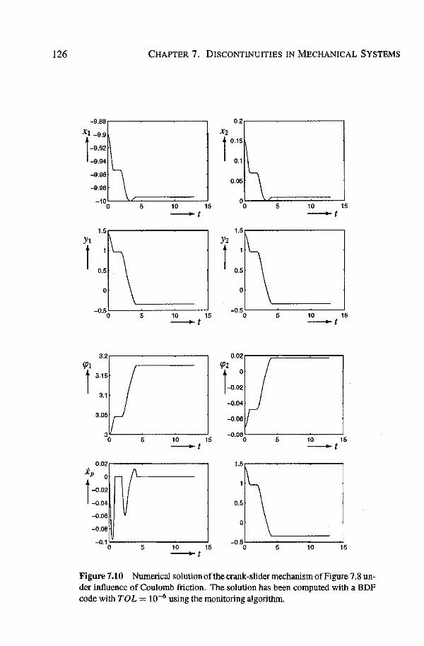
126 CHAPTER 7. DISCONTINUITIES IN MECHANICAL SYSTEMS

-9.88 0.2

xz l 0.15

''t\ 0.05

0 15 5 10 15 0 5 10

-t _,

YI Yz

l t

-0.5 0 5 10 15

-0.5 0 5 10 15

-t -t

3.2 0,02 ({Jt ({Jz

t l-0.0:

5 10 15 5 10 15 -t ·-t

0.02 Xp

0

~r ,-0.02

-0.04

-0.06

-0.08

-0.1 0 5 10 15 -0.5o~----~5------,o----~,5

-t

Figure 7.10 Numerical solutionofthecrank-slidermechanismofFigure 7.8 un­der infiuence of Coulomb friction. The solution has been computed with a BDF code with TOL= 10-6 using the monitoring algorithm.

8 CONCLUSIONS AND

DISCUSSION

8.1 CONCLUSIONS

As stated in Section 1.4 the direct reason for the investigation described in this thesis was to develop a reliable and efficient numerical metbod for solving the equations of motion of multibody systems, in particular for systems with closed loops. Multibody dynamics often give rise to differentlal equations with forcing functions exhibiting discantinuitles in the form of finite jumps, either in the function themselves or in some derivatives of them. As a consequence, the salution metbod should adapt to these discantinuitles in order to simulate multibody systems exhibiting discontinuities in an efficient and robust manner.

The equations of motion descrihing the dynamics of multibody systems can be de­rived in two different ways. The first metbod is the so-called augmentation method. lt uses a global coordinate description and adds the constraint equations (describing the intercounections between bodies) to the dynamic equations (i.e. differentlal equations), resulting in a system of differentlal algebraic equations (DAEs). Using this metbod the equations of motion are obtained in the descriptor form. The second metbod is the so­called eliminadon approach. lt uses relative (independent) coordinates. For open loop systems (where the bodies are connected in a unique way) both the constraint farces and the constraint equations can be eliminated. The equations of motion then form a sys­tem of ordinary differentlal equations (ODEs). Closed loop systems (where the bodies are not connected in a unique way), however, also result in a system of DAEs using the elimination method, since additional constraints have to be satisfied.

Quite often in practice, DAEs appear in a form where the algebraic equations and the differentlal equations are explicitly given. Such systems are so-called semi-explicit DAEs. The DAEs descrihing the multibody dynamics are such semi-explicit systems. The nature of DAEs is described by the index, which appears to characterize the numer­ical difficulty of a DAE. ODEs are DAEs of index zero, and the equations of motion of

128 CHAPTER 8. CONCLUSIONS AND DISCUSSION

multibody systems are DAEs of index three. In this thesis we have studied the conditioning, i.e. the sensitivity of the salution to

perturbations in the system, of semi-explicit DAEs of index one and two. The matrices D, for index one DAEs ( cf. Chapter 4), and CB, for index two DAEs ( cf. Chapter 5), natu­rally appear when determining the dependency of the algebraic variabie as function of the differential variables. Conditioning results in literature suggest that some conditioning constauts depend on the norm of the inverse of these matrix coefficients, implying that these constauts grow unboundedly when these matrices become almast singular. This means that small perturbations in the initial values or the forcing functions may result in large errors in the solution. In the Chapters 4 and 5 we have shown that such DAEs may behave almast like associated DAEs of higher index. Under the assumption that these associated higher index DAEs are well-conditioned themseives, appropriate sta­bility constauts of the latter are of moderate size. We have proven in this study that the conditioning constauts of the index one and index two DABs with almast singular ma­trices D and CB, respectively, also remain moderately sized then. As a consequence, no larger errors will appear in the solution. By this we are able to determine the effective index of the variables and we give a metbod to determine, at least theoretically, the effec­tive index of the variables. Moreover, it bas been shown that the conditioning constauts will grow unboundedly for DAEs that are not close to a well-conditioned higher index DAB. In addition we have shown fot DAEs of index two and higher that perturbations of the coefficients may have a dramatic impact on the salution behaviour, whereas for DAEs of index zero and one this phenomenon does not occur.

As stated earlier, the index of a DAB characterizes the numerical difficulty of it. Most numerical methods are convergent for index one systems only and a loss of the accuracy may occur in the algebraic variables (i.e. those variables for which no differential equa­tion is given directly). Methods based on backward differentiation formulae, so-called BDP methods, converge forsome important classes of DAEs of index higher than one. The equations of motion for multibody systems, which have index three, belang to such a class. Applying BDP methods tothese higher index DAEs results in ill-conditioned it­eration matrices. The conditioning of iteration matrices bas been studied in Section 6.2. This ill-conditioning implies that rounding errors and errors due to linearizations are am­plified by negative powers ofthe step-size h (see Section 6.2) in the numerical approx­imation of the algebraic variables. Por more general DAEs, however, mixing of errors from the dynamic and the algebraic part can occur, implying that the dynamic variables are affected also. Hence, larger errorscan appear in the approximations. We have shown that, for (lower index) DAEs which are almast higher index, this amplification effect will be worse than expected on ground of that lower index. Numerical evidence illustrates that the amplification of rounding errors in the numerical approximation commensurates with the theoretica! conditioning results obtained in Subsection 6.2.2. Por variabie step, variabie order BDP methods this ill-conditioning results in an erratic behaviour of the step-size control mechanism and the Newton iterations. As a consequence, these BDP methods might even fail integrating DAEs of index one. As suggested in literature, this can be remedied by sealing of the error estimates, both in the local error estimation and in the estimation of errors in the Newton iterations. Using these modifications means

8.2. DISCUSSION 129

that DAEs of higher index can be solved numerically in this higher index form directly. A particular projection metbod (6.12) combined with these modifications of the BOF metbod result in a rather efficient metbod for solving DAEs of higher index.

Discontinuities, e.g. due to impacts, hysteresis and Coulomb friction, arise frequently in the simulation of multibody systems. The appearance of such discontinuities causes severe problems during the numerical solution process; numerical solution methods may become very inefficient or may even fail during the passage of discontinuities. We have implemented a metbod to handle such discontinuities in an efficient way by using switch­ing functions (see also [19, 43]). The use of these functions providesus a means to lo­calize the discontinuity. Next we determine how the solution behaves near the discon­tinuity. When the solution passes the so-called manifold of discontinuity, the solution moves beyond the discontinuity and a new forcing function bas to be considered. On the other hand, if the solution stays in the manifold of discontinuity (which may hap­pen when a mechanical system with Coulomb friction switches from the slip phase to the stick phase for example), the OAE bas to be augmented by constraining equations as well as constraint forces in order to keep the system in the manifold of discontinuity. Numerical examples studied in Chapter 7 show that this provides for an appropriate tooi for the simulation of mechanical systems exhibiting discontin ui ties.

8.2 DISCUSSION

A subject for further development is the reduction of the amount of work in the linear algebra, which can be attained by exploring on the structure of the equations of motion for multibody systems. Especially in larger systems one can explore the sparseness of the system of linear equations when f{)rmulating the equations in descriptor form (cf. Chapter 2).

The numerical results for the solution of the eqnations of motion of multibody sys­tems presented in Chapters 6 and 7 have been obtained by application of the descrip­tor form ( cf. Chapter 2). To solve multibody systems with closed loops using the C> ( n )­recursive formalism for the generation of the equations of motion as elaborated in Chap­ter 2 bas appeared to be suitable for large-scale open loop systems. Still, a subject for further study is the use of this formalism for closed loop systems.

The simulation illustrated in Figure 1.2 of Chapter 1 suggests the importance of han­dling multibody systems consisting not only of rigid bodies but also of flexible bod­ies. Induced by the increasing interest in deformable bodies, the development of C>(n)­recursive methods (cf. Chapter 2) overlaps with the research actlvities on the modelling and the simulation of flexible bodies, cf. [16, 51-53]. Almost all approaches hitherto are based on the major assumption that the elastic deformations are small. One may use any multibody system formalism to generate the equations of motion. These equations are generated in the same form as for rigid bodies, but extra unknowns in the form of modal coordinates, accounting for the modal modes, have to be introduced into the sys­tem. In [51, 52] the C> (n )-recursive metbod for generating the equations of multibody systems consisting of rigid bodies bas been extended to a treatment of flexible bodies;

130 CHAPTER 8. CONCLUSIONS AND DISCUSSION

bere the deformation modal coordinates are defined as generalized coordinates, i.e. the mass of the body is concentrated on certain nodes with elasticity remaining continuous. As a consequence, the resulting mechanica! systems consisting of flexible bodies are more stiff than the systems constituted of rigid bodies only. Hence, a topic for further research is the study of the effects of incorporating flexibility on the numerical solution of the equations of motion of multibody systems.

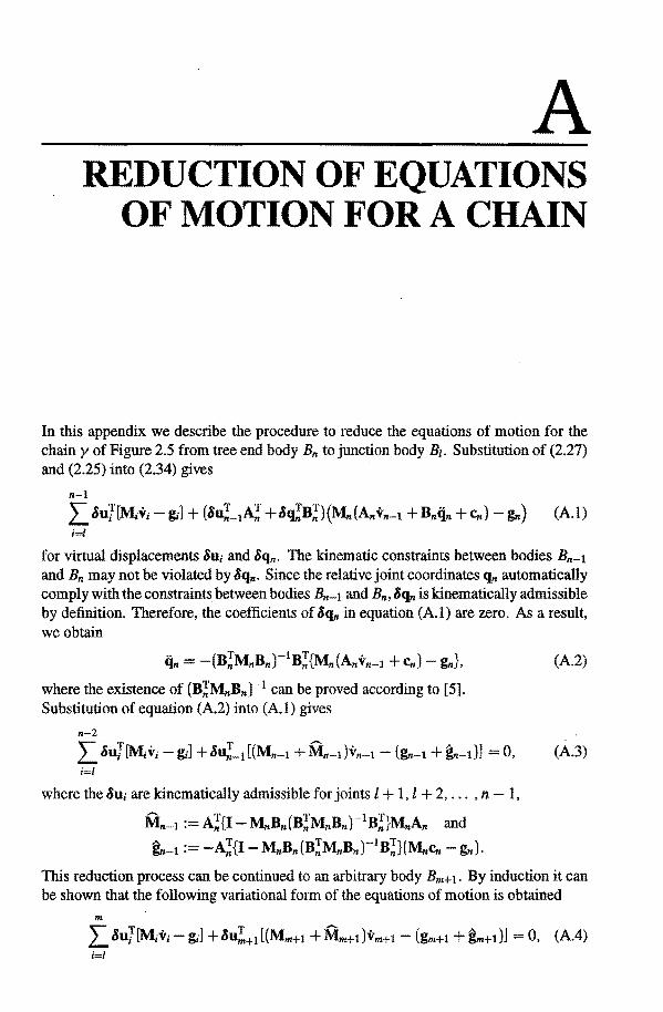
A REDUCTION OF EQUATIONS

OF MOTIONFORA CHAIN

In this appendix we describe the procedure to reduce the equations of motion for the chain y of Figure 2.5 from tree end body En to junction body B1• Substitution of (2.27) and (2.25) into (2.34) gives

n-1 L &uj[M;v;- g;] + (&u!'-tA! +&'J!B!){Mn(AnVn-1 + Bnéin + Cn) ~} (A.l) i=l

for virtual displacements &u; and &qn. The kinematic constraints between bodies Bn-1 and Bn may not be violated by &qn. Since the relative joint coordinates qn automatically comply with the constraints between bodies Bn-1 and Bn. &qn is kinematically admissible by definition. Therefore, the coefficients of &qn in equation (Al) are zero. As a result, we obtain

éin = -(B!MnBn)-1B!{Mn(AnVn-1 +Cn) ~}.

where the existence of (B!MnBn)-1 can be proved according to [5]. Substitution of equation (A2) into (Al) gives

n-2

(A2)

L &uj[M;v;- g;] + &n!-1 [(Mn-1 + Mn-dVn-1 - (~-1 + ~-1 )] = 0, (A.3) i= I

where the &u; are kinematically admissible for joints l + 1,1 + 2, ... , n- 1,

Mn-t := A!{I- MnBn(B!MnBnt1 B!}MnAn and

~-1 := -A!{I- MnBn(B!MnBn)-1B!}(Mncn- ~).

This rednetion process can be continued to an arbitrary body Bm+ 1• By induction it can be shown that the following variational form of the equations of motion is obtained

m

L &u[[M;v;- g;] + &n~+l [(Mm+l + Mm+l )vm+l - (gm+l + @m+t )] = 0, (A4) i=l

132 APPENDIX A. RBDUCTION OF EQUATIONS OF MOTION POR A CHAIN

where virtual displacements &ui, i l, l + 1, ... , m + 1, are k.inematically admissible for joints between bodies Bz to Bm+l· However, they are free from kinematica! admissi­bility conditions corresponding to constraints between bodies Bm+t to Bn. because these constraints are satisfied by the relative coordinates.

Substituting equations (2.25) and (2.27), with i= mand j m + 1, into (A4) results in

m-1

L &uj(M;v; ~) +óu~[A~+l{(Mm+l +Mm+IHAm+tVm +Bm+l<.im+l i=l

+cm+l)- (~+1 +~+t)}+MmVm- ~] +8~+1B~+l{(Mm+l

+Mrn+t)(Am+lVm +Bm+liim+l +cm+l)- (~+1 +~+1)} =0,

(A5)

for k.inematically admissible &u;, i I, ... , m, and &qm+l· Once more, 8qm+1 is kine­matically admissible by definition. As &ui, i= l, ... , m, and 8qm+l are independent, the coefficient of &qm+t in equation (A5) must be equal to zero, resulting in

iim+l = -(B~+l (Mm+l + Mm+l)Bm+tr1B~+l{(Mm+l + Mm+tHAm+tVm +cm+l)- (gm+l +~+1)}.

As before, according to [5], the existence of

(B~+I (Mm+t + Mm+I)Bm+tr1

can be proved. Substituting (A6) back into (A5) gives

m-1

L &uj[M;v;- g;] + &u~[(Mm + Mm)Vm- (~ + im)l = 0, i=l

and

(A6)

and, &u; is kinematically admissible for joints between bodies Bt to Bm. This reduction processcan be continued to junction body Bt. Now, the reduced variational equations of motionread

T ..-.. &ur [(Mr + MDvt - (gt + inl = o,

where &ut is ~nematically admissible for all extemal constraints that act on junction body Bt, and Mf and ir follow from equations (A 7) and (A.8), respectively, with m = l.

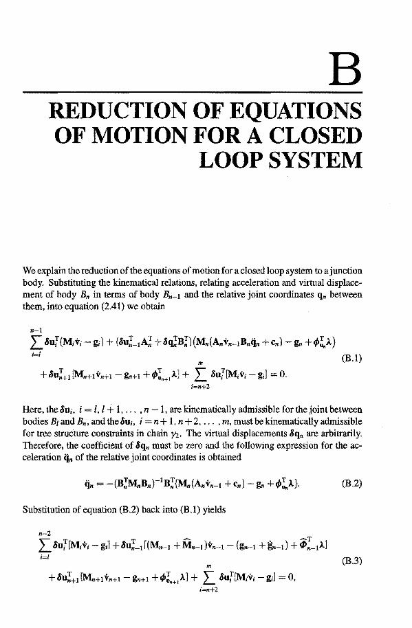
B REDUCTION OF EQUATIONS OF MOTIONFORA CLOSED

LOOPSYSTEM

We explain the reduction of the equations of motionfora closed loop system toa junction body. Substituting the kinematical relations, relating acceleration and virtual displace­ment of body Bn in terms of body Bn-l and the relative joint coordinates q,. between them, into equation (2.41) we obtain

n-l L &uj(M{V; -g;) + (&u!-ti\J +&~B;!'){Mn(AnVn-tBniin +Cn) -~+</{A.) i=l

m (B.l)

+&u!'+tlMn+lvn+t- ~+1 +4{+1Ä] + L &uj[M;v;- g;] = 0. i=n+2

Here, the&ui, i= l, l + 1, ... , n -1, arekinematically admissible forthejoint between bodies Bz and Bn, and the&u;, i =n+ 1, n +2, ... , m, mustbekinematically admissible fortree structure constraints in chain )12. The virtual displacements &qn are arbitrarily. Therefore, the coefficient of &qn must be zero and the following expression for the ac­celeration iin of the relative joint coordinates is obtained

Substitution of equation (B.2) back into (B.l) yields

m (B.3)

+&u!'+t [MnHVn+l- ~+1 +4{+1Ä] + L &uj[M;v;- g;] = 0, i=n+2

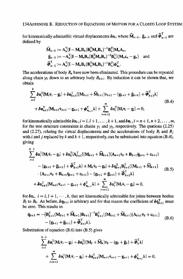
134APPENDIX B. RBDUCTION OF EQUATIONS OF MOTIONFORA CLOSBD LOOP SYSTBM

for kinematically admissible virtual displacements Su1, where Mn-1, ~-1 and i!_1 are defined by

Mn-t := A~{I- MnBn(BJM,.Bn)-1B~}M"A,., ~-1 :=-~{I- MnBn (B~MnBn)-1 B~}(MnCn - g,.) and

--T T{ ( T B )-1 Tu..T *"'n-1 :=AnI MnBn BnMn n BnN'Un·

The accelerations of body Bn have now been eliminated. This procedure can be repeated along chain y1 down to an arbitrary body Bk+l· By induction it can be shown that, we obtain

k

L. SuJ[M;v;- g;l +&ui +I [(Mk+t + M:k+I )vk+1 - (~+I + @k+1) + i>J+11] i=l

m

+Su~+trMn+tVn+I-g,.+t +t/{+1À] + L &uJ[M;v;-g;] =0, i=n+2

(B.4)

forkinematicallyadmissible&ui.i =l, l + 1, ... , k+ 1, and&u;, i =n+ l,n+2, ... , m, forthetree structure constraints in ebains y1 and )12, respectively. The quations (2.25) and (2.27), relating the virtual displacements and the accelerations of body B; and Bi with i and j replaced by k and k + 1, respectively, can be substituted into equation (B.4), giving

k-1

L &uJ[M;v;- g;] +&uJ[AJ+tHMk+t + ~+t)(Ak+tvk + Bk+té:ik+t + Ck+d i=l

m

+ &u~+l [Mn+l Vn+I - g,.+l + lP~+l À] + L &uJ[M;v; - g;] = 0, i=n+2

(B.5)

for &u;, i = l, l + 1, · · · , k, that are kinematically admissible for joints between bodies B1 to Bk. As before, &qk+l is arbitrary and for that reason the coefficient of SqJ+l must be zero. This results in

é:ik+t =-(BJ+l(Mk+t +Mk+t)Bk+tr1BJ+l{(Mk+l +~+t)(Ak+tVk+ck+t)

--T (B.6) - (~+1 +~+t) +~k+lÀ}.

Substitution of equation (B.6) into (B.5) gives

k-1

L &uj[M;v; - g;] + &uJ[(Mk + Mk)-vk i=l

m

+ L &u{[M;v;-g;] +&uJ+trMn+Ivn+I-g,.+l +lP~+1 l.] =0, i=n+2

135

where

..- T ..- ( T )-1 T Mk := Ak+1{1- (Mk+l + Mk+t)Bk+t Bk+l (Mk+l + ~+l)Bk+l Bk+1 (Mk+t

+ Mk+dAk+t}, T """ ( T ........ )-1 T ~ := -Ak+l{I- (Mk+l + Mk+t)Bk+l Bk+1 (Mk+l + M.t+t)Bk+l Bk+l}

· (Mk+t +Mk+t)Ck+l- (~+1 +~+1)} and

•! :=AI+t{I- (Mk+t +M+t)Bk+t(BI+t(~+1 +Mk+dBk+lf1BI+tJ4>!+t·

This procedure can be performed for each chain in the spanning tree from each cut joint body to the first junction body encountered and will result in the following equation for the junction body.

136APPENDIX B. REDUCTION OF EQUATIONS OF MOTIONFORA CLOSED LOOP SYSTEM

c RELATION BETWEEN THE

FUNDAMENTAL SOLUTION AND THE GREEN FUNCTION

OF ANODE AND A SLIGHTLY PERTURBED ONE

Consider the IVPs

y' = Ay + f, with y(to) = fJ, (C.l)

and the perturbed IVP

z' Áz + f, with z(to) = fJ, (C.2)

where

Ä =A+6A, andf=f+Sf.

Then (C.2) yields

z' =Az+f+8Az+6f, withz(to) =fJ.

Let tiJ, i/J denote the fundamental solutions of (C.l ), (C.2), respectively. Then, the solu­tion of (C.2) is given by

z(t) = ib(t)fJ +ft i/J(t)ib-1 (s)f(s)ds to

= tP(t)fJ + J: t/J(t)t/J-1(s)(8A(s)z(s) + f(s) +6f(s))ds

=tP(t)fJ+ I: t/J(t)4>-1 (s)(8A(s)z(s) +Ï(s))ds

As a consequence,

ib(t) = t/J(t) +ft t/J(t)t/J-1 (s)6A(s)ib(s)ds. (C.3) to

138 APPENDIX C. RELATION BETWEEN FUNDAMENTAL SOLUTIONS

Let G(t, s) and G(t, s) denote theGreenfunctions of(C.l) and (C.2), respectively. Then

G(t, s) G(t, s} + .P(t)G(O, t) - Jt G(t, s )8A(s )G(t, s )ds. (C.4) to

With the definition

the aforementioned relations make it possible to compare the conditioning constants of the two neighbouring problems (C.l) and (C.2). If tez8A < 1, then

(C.5)

This means that a well conditioned NP remains reasonably conditioned if A and the ini­tia! conditions are pertuebed only slightly. From relations (C.3) and (C.4) we can con­clude that iiJ and cP may differ a lot if II&AII is large. The same holds for G and G.

REFERENCES

[1] W. ARMSTRONG. Recursive solution to the equations of motion of an n-link ma­nipulator. In Proc. 5th World Congress on Theory of Machines and Mechanism (Montreal, 1979), vol. 2, pp. 1343-1346.

[2] U. AscHER. On symmetrie schemes and differentlal algebraic equations. SIAM Joumal Sci. Stat. Comp JO (1989), 937-949.

[3] U. ASCHER AND L. R. PETZOLD. Projected implicit Runge-Kutta for differentlal algebraic equations. SIAM J. Numer. Anal. 28 (1991), 1097-1120.

[4] U. AseHER AND L. R. PETZOLD. Stability of computational methods for con­strained dynamics systems. SIAM Joumal Sci. Comp 14, 1 (1993), 95-120.

[5] D. BAE AND E. J. HAUG. A recursive formulationfor constrained mechanical sys­tem dynamics: Part I, open loop systems. Mechanics of Structures and Machines 15, 3 (1987), 359-382.

[6] D. BAE AND E. J. HAUG. Arecursiveformulationforconstrainedmechanicalsys­tem dynamics: Part 11, closed loop systems. Mechanics of Structures and Machines 15,4 (1987), 481-506.

[7] J. BAUMGARTE. Stabilization of constraints and integrals of motion in formulae. Computer Methods inAppliedMechanics andEngineerring. 1 (1972), 1-16.

[8] P. BRASEY. Maximimum weighted matchingfor high index differential algebraic equations. PhD thesis, Delft University ofTechnology, Delft, 1994.

[9] K. E. BRENAN, S. L. CAMPBELL, AND L. R. PETZOLD. Numerical Solution of Initia/-Value Problems in Differential Algebraic Equations. North-Holland, New York, 1989.

140 REPERENCES

[10] K. E. BRENAN AND B. E. ENGQUIST. Backward differentlation approximations of nonlinear differentlal algebraic equations, and supplement. Math. Comp. 51 (1988), 659-676.

[11] K. E. BRENAN AND L. R. PETZOLD. Numerical solutionofnonlineardifferential equations with algebraic constraints i: Convergence resu1ts for backward differen­tlation formulas. Math. Comp. 46 (1986), 491-516.

[12] K. È. BRENAN AND L. R. PETZOLD. Numerical solution of nonlinear differentlal equations with algebraic constraints ii: Practical implementations. SIAM J. Sci. Stat. Comp. 7 (1986), 720-733.

[13] J. C. BUTCHER. The Numerical Analysis of Ordinary Differential Equations: Runge-Kutta and generallinear methods. John Wtley & Sons, Chichester, 1987.

[14] S. L. CAMPBELL. Singular Systems of Differential Equations. Pitman, London, 1980.

[15] M. CHACE. Methods and experience in computer aided design of large'" displacement mechanical systems. In Computer Aided Analysis and Optimization of Mechanica[ System Dynamics (Heidelberg, 1984), E. Haug, editor, Springer­Verlag.

[16] K. CHANGIZI AND A. A. SHABANA. A recursive formu1ation for the dynamic analysis of open loop deformable mul ti body systems. Joumal of Applied Mechan­ics 55 (1988), 687-693.

[17] G. DAHLQUIST AND A. BJÖRK. Numerical Methods. Prentice-Hall, Englewood Cliffs, New Jersey, 1974. Translated by N. Anderson.

[18] P. DEUFLHARD, E. HAIRER, AND J. ZUGCK. One-step andextrapolationmethods for differential-algebraic systems. Num. Matk 51 (1987), 501-516.

[19] E. EICH. Projizierende Mehrschrittverfahren zur numerischen Lösung von Bewe­gungsgleichungen technischer Mehrkörpersysteme mit Zwangsbedingungen und Unstetigkeiten. PhD thesis, Universität Augsburg, 1992. In German.

[20] E. EICH. Convergence results for a coordinate projection metbod applied to me­chanica! systems with algebraic constraints. SIAM J. Num. Analysis 30,5 (1993), 1467-1482.

[21] E. EICH, C. FÜHRER, B. J. LEIMKUHLER, AND S. REICH. Stabilizationandpro­jection methods for multibody dynamics. Tech. rep., Helsinki University of Tech­nology, 1990.

[22] E. EICH AND HANKE. Regularization methods for constrained mechanics systems. Tech. rep., Humboldt-Universität zu Berlin, 1991.

REPERENCES 141

[23] A. BICHBERGER, C. FÜHRER, AND R. SCHWERTASSEK. The benefits of parallel multibody simulation and its application to vehicle dynamics. InAdvanced Multi~ body System Dynamics (Dordrecht, 1993), W. Schiehlen, editor, Kluwer Academie Publishers.

[24] W. H. BNRIGHT, K. R. JACKSON, S. P. N0RSETT, AND P. G. THOMSEN. Bffec~ tive salution of discontinuons IVPs using a Runge~Kutta formula pair with inter~ polants. Appl. Math. and Comput. 27 (1988), 313-335.

[25] A. F. FILIPPOV. Differentlal equations with discontinuons right-hand sides. ACM Trans!. 42 (1964), 199-231.

[26] 0. FISCHER. Theoretische Grundlagen für eine Mechanik der lebenden Körper. Teubner, Berlin, 1906.

[27] C. FüHRER. DijferentialAlgebraische Gleichungsysteme in Mechanischen Mehr~ körpersystemen. PhD thesis, Technische Universität München, München, 1988.

[28] C. FÜHRER AND B. J. LEIMKUHLER. Pormulation and numerical solution of the equations of constrained motion. Tech. Rep. DFVLR~FB 89-08, DFVLR, Oberp~ faffenhofen, West-Germany, 1989.

[29] C. FüHRER AND B. J. LEIMKUHLER. A new class of generalized inverses for the solution of discretized Buler-Lagrange equations. In Real-Time Integration Meth­ods for Mechanica! System Simulation (Berlin, 1991), B. J. Haug and R. C. Deyo, editors, numberDFVLR-FB 89-08, NATO ASI Series, Springer-Verlag.

[30] F. R. GANTMACHER. The Theory of Matrices. Chelsea, 1959.

[31] C. W. GEAR. The simultaneons numerical salution of differential-algebraic equa­tions. IEEE Trans. Circuit Theory CT-18 (1971), 89-95.

[32] C. W. GEAR. Differentlal algebraic equation index transformations. SIAM 1 Sci. Stat. Comp. 9 (1988), 39-47.

[33] C. W. GEAR. Differentlal algebraic equations, indices, and integral algebraic equa­tions. SIAM 1 Numer. Anal. 27,6 (1990), 1527-1534.

[34] C. W. GEAR, G. K. GUPTA, AND B. J. LEIMKUHLER. Automatic integration of Buler-Lagrange equations with constraints. 1 Camp. Appl. Math. 12&13 (1985), 77-90.

[35] C. W. GEAR, H. H. Hsu, AND L. R. PETZOLD. Differentlal algebraic equations revisited. In Proc. ODE Meeting (Oberwolfach, West Germany, 1981).

[36] C. W. GEAR AND 0. 0STERBY. Solving ordinary differentlal equations with dis­continuities. ACM Trans. Math. Softw. 10 (1984), 23-44.

142 REPERENCES

[37] C. W. GEAR AND L. R. PETZOLD. Ode methods for the solution of differential algebraic systems. SIAM 1 Numer. Anal. 21 (1984), 367-384.

[38] G. H. GOLUB AND C. F. V. LOAN. Matrix Computations. John Hopkins Univer­sity Press, Baltimore, 1990.

[39] D. T. GREENWOOD. Principlesof Dynamics. Prentice-Hall, Inc., Engtewood Cliffs, New Jersey, 1965.

[ 40] E. GRIEPENTROG AND R. MÄRZ. DijferentialAlgebraic Equations and Their Nu­merical Treatment, vol. 88. Teubner-Texte zur Math., Leipzig, 1986.

[4l.] E. HAIRER, C. LUBICH, AND M. ROCHE. Numerical Solution of Dijferential-Algebraic Systems by Runge-Kutta Methods. Lecture Notes in Math. 1409. Springer-Verlag, Berlin, 1989.

(42] E. HAIRER, S. P. N0RSETT, AND G. WANNER. Solving Ordinary Dijferential Equations I, Nonstijf Problems, second revised edition. Springer-Verlag, Berlin, 1993.

[43] E. HAIRER AND G. WANNER. Solving Ordinary Dijferential Equations I[, Stijf and Dijferentia!Algebraic Problems. Springer-Verlag, Berlin, 1991.

[ 44] J. P. HARTOG DEN. Forced vibrations with combined viscous and coulomb damp­ing. Phil. Mag. Ser. 7 9 (1930), 801-817.

[ 45] E. J. HAUG. Computer-Aided Kinematics and Dynamics of Mechanica[ Systems. Allyn and Bacon, Boston, 1989.

[46] E. J. HAUG, P.E. NIKRAVESH, V. N. SOHONI, AND R. A. WEHAGE. Computer aided analysis of large scale, constrained, mechanica! systems. In 4th International Symposium on Large Engineering Systems (Calgary Alberta, Canada, 1982).

[47] E. J. HAUG AND J. YEN. Generalized coordinate partitioning methods for nu­merical integration of differential algebraic equations of dynamics. In Real-nme Integration Methods for Mechanica[ System Simulation (Berlin, 1991), E. J. Haug and R. C. Deyo, editors, NATO ASI Series, Springer-Verlag.

[ 48] A. C. HINDMARSH. LSO DE and LSO DI, two new initia! value ordinary differen­tial equation solvers. ACM-SIGNUM, Newslette 15 (1980), 10-11.

[49] W. HOOKER AND C. MARGULIES. The dynamical attitude equations for an n­body satellite. 1 Astronaut. Sci. 12 (1965), 123-128.

[50] R. HUSTON. Useful procedures in multibody dynamics. In Proceedings of the lU­TAM!IFToMM SymposiumonDynamics ofMultibody Systems (Udine, Italy,l985), G. Bianchi and W. Schiehlen, editors, pp. 69-77.

REPERENCES 143

[51] S. S. KIM AND E. J. HAUG. A recursive fornlUlation for fiexible multibody dy­namics: Part I. open loop systems. Computer Methods in Applied Mechanics and Engineerring. 71 (1988), 293-314.

[52] S. S. KIM AND E. J. HAUG. A recursive formulation for fiexible multibody dy­namics: Part II. closed loop systems. Computer Methods inApplied Mechanics and Engineerring. 74 (1989), 251-269.

[53] W. KOPPENS. The Dynamics ofSystems ofDeformable Bodies. PhD thesis, Eind­hoven University ofTechnology, 1989.

[54] M. LENTINI AND R. MÄRZ. The conditioning of boundary value problems in transferable differential-algebraic equations. SIAM J. Numer. Anal. 27, 4 (1990), 1001-1015.

[55] P. M. LOON VAN. ContinUDus decoupling transformations for linear boundary value problems. PhD thesis, Eindhoven University of Technology, Eindhoven, 1987.

[56] C. LUBICH, U. NOWAK, U. PÖHLE, AND C. ENGSTLER. MEXX - numerical software for the integration of constrained mechanica! multibody systems. Tech. Rep. Preprint SC 92-12, Konrad-Zuse-Zentrum führ Informationstechnik: Berlin, Berlin, December 1992.

[57] D. G. LUENBERGER. Dynamic equations in descriptor form. IEEE Trans. Auto­matic Control22 (1977), 312-321.

[58] H. A. LUPKER, P. J. S. DE Coo, AND J. WISMANS. Advances in MADYMO crash simulations. SAE 910879, International Congress and Exposition.

[59] R. MÄRZ AND C. TISCHENDORF. Solving more general index-2 differential al­gebraic equations. Tech. Rep. 93-6, Humboldt Universität zu Berlin, 1993.

[60] R. R. M. MATTHEIJ AND J. MOLENAAR. Ordinary dijferential equations in the­ory and practice, Analysis, Numerical Methods, Mathematica! Model/ing. John Wiley & Sons Ltd., Chichester, 1996.

[ 61] R. E. 0' MALLEY. On nonlinear singularly perturbed initia! value problems. SIAM Rev. 30 (1988), 193-212.

[ 62] R. E. 0' MALLEY. Singular Perturbation Methods for Ordinary Dijferential Equa­tions. Springer-Verlag, New York, 1991.

[63] N. ORLANDEA. Node-Analogous, Sparsity-Oriented Methods for Simu/ation of Mechanica/ Systems. PhD thesis, University of Michigan, 1973.

[64] N. 0RLANDEA, M. A. CHACE, AND C.A. CALAHAN. A sparsity-oriented ap­proach to the dynamic analysis and design of mechanical systems. J. Engng. lnd. 99 (1977), 773-784.

144 REPERENCES

[65] L. R. PETZOLD. Differentlal algebraic equations are not ODEs. SIAM 1 SC!. Stat. Comput. 3, 3 (1982), 367-384.

[ 66] L. R. PETZOLD. A description ofDASSL, a differentlal algebraic system solver. In Scientijic Computing: Applications ofMathematics and Computing to the Physical Sciences (Amsterdam, 1983), R S. S. et al., editor, North-Holland, pp. 65-68.

[ 67] L. R. PETZOLD. Order results for impHeit Runge-Kutta methods applied to differ­entlal algebraic systems. SIAM 1 Numer. Anal. 23 (1986), 837-852.

[68] L. R. PETZOLD AND P. LöTSTEDT. Numerical solution of nonlinear differentlal equations with algebraic constraints ii: Practical implications. SIAM 1 Sci. Stat. Comput. 7 (1986), 720-733.

[69] F. A. POTRA AND W. C. RHEINBOLDT. On the numerical solution of the Buler-Lagrange equations. In Re al-Time lntegration Methods for Mechanica/ Sys­tem Simulation (Berlin, 1991), E. Haug and R Deyo, editors, NATO ASI Series, Springer-Verlag.

[70] R. REISSIG. Erzwungene Schwingungen mit zäher un trackener Reibung. Math. Nachr. 11 (1954), 345-384.

[71] W. C. RHEINBOLDT. On the existence and uniqueness of solutions of nonlinear semi-impHeit differentlal algebraic equations. Nonl. Analysis, Theory, Methods & Applications 6, 7/8 (1991), 647-661.

[72] R. E. ROBERSON. The path matrix of a graph, its construction and its use in evalu­ating certain products. Computer Methods in Applied Mechanics and Engineering 24 (1984), 47-56.

[73] R. E. ROBERSON AND R. SCHWERTASSEK. Dynamics of Multibody Systems. Springer-Verlag, Berlin, 1988.

[74] R. SCHWERTASSEK AND W. RULKA. Aspectsof efficient and reliable multibody system simulation. In Re al-Time Integration Methods for Mechanica[ System Sim­u/ation (Berlin, 1991), E. Haug and R. Deyo, editors, NATO ASI series, Springer­Verlag.

[75] L. F. SHAMPINE. Conservalion laws and the numerical salution of ODE's. Comp. and Maths. with Appls. 12 (1986), 1287-1296.

[76] P. M. A. SLAATS. Recursive formulations in multibody dynamics. Tech. rep., IVO, Eindhoven University of Technology, Eindhoven, 1991.

[77] D. STEWART. A high accuracy metbod for solving ODEs with discontinuous right­hand side. Numer. Math. 58 (1990), 299-328.

REPERENCES 145

[78] K. TAUBERT. Differenzverfahren für Schwingungen mit trackenerund zäher Rei­bung und für Regelungssysteme. Numer. Math. 26 (1976), 379-395.

[79] A. F. VERESHCHAGIN. Computer simulation of the dynamics of complicated mechanisms of robot-manipulators. Engng. Cybernetics 6 (1974), 65-70.

[80] R. A. WEHAGE AND E. J. HAUG. Oeneralized coordinate partitioning for dimen­si on rednetion in analysis of constrained mechanica! systems. J. of Mechanical Design 104 (1982).

[81] P. M. E. J. WIJCKMANS. Multibody systems. RANA Report of the Department of Mathernaties and Computing Science 92-10, Eindhoven University ofTechnology, 1992.

[82] P. M. E. J. WIJCKMANS. Differentlal algebraic equations. RANA Report of the Department of Mathernaties and Computing Science 93-02, Eindhoven University of Technology, 1993.

[83] P.M. E. J. WIJCKMANS AND R. M.M. MATTHEIJ. Discontinuities in mechan­ica! systems. In Proceedings of the Sixth Colloquium on Differential Equations (Plovdiv, 1996). To appear.

[84] J. WITTENBURG. Dynamics ofSystems ofRigid Bodies. Teubner, Stuttgart, 1977.

146 REPERENCES

c:>(n)-formulations, 25

absolute angular ve1ocity, 13 absolute coordinates, 5 absolute position, 13 absolute variables, 5 acceleration constraints, 17 ADAMS, 18 algebraic variables, 37 augmentation method, 5, 11

backward difference formulae, 41 base body, 20 Baumgarte parameters, 86 Baumgarte stabilization, 86 BDF,41 body conneetion array, 20

canonical projector, 50 center of mass, 13 chain, 21 close to higher index DAB, 60 closed chain, 6 closed loop, 19, 26 closed loop system, 6, 11 composite generalized coordinates, 15 composite generalized 1oad, 15 composite generalized mass, 15 conditioning, 10,12,49,51 conditioning constants, 51

INDEX

configuration, 14 consistent initial conditions, 32 constrained equations of motion, 17 constrained variational equations of mo-

tion, 15 constraint, 4

holonomic constraint, 15 nonholonomic constraint, 15

constraints acceleration constraints, 17 position constraints, 17 velocity constraints, 17

coordinate projection methods, 89 cut joint, 6, 7, 11 cut joints, 21

d' Alembert's principle of virtual work, 15

DADS, 18 DAB, 6, 8, 31 derivative projection methods, 89 descriptor form, 5, 11, 17 differential algebraic equation, 6, 8, 31 differential index, 11, 35 differential variables, 37 direct approach, 43 drift, 85' 87 dynamic analysis, 2 dynamic variable, 52

148

edges, 20 effective index, 64 elimination method, 5, 11 equations of motion , 16

father, 20 fundamental solution, 50

generalized applied loads, 15 generalized constraint loads, 15 generalized coordinate partitioning, 88 generalized coordinates, 7, 14 generalized loads

generalized applied loads, 15 generalized constraint loads, 15

generalized singularvalue decomposition, 65

generating polynomials, 41 GSVD,65

Hessenberg form, 45 holanomie constraint, 15

implicit DAE, 36 implicit Runge-Kutta, 46 index, 9, 11

differentlal index, 11 perturbation index, 11 index of nilpotency, 33

indirect approach, 43 inertia matrix, 13 IRK,46

joint, 14 joint coordinates, 6

kinematically admissible displacement, 15

Lagrange equations of type two, 4 Lagrange multiplier, 4, 6, 11, 16 Lagrange's equations of type one, 17 local index, 35

machine precision, 92 manifold of discontinuity, 108 mass, 13

INDEX

matrix pencil, 32 metbod of Lagrange multipliers, 11, 16 multibody formalism, 4 multibody system, 1 multistep method, 11, 40

nodes, 20 nonholonomic constraint, 15

ODAE,90 ODE,6 openloop, 19 open loop system, 6, 11 ordinary differentlal equations, 6 overdetermined DAE, 90

perturbationindex, 11,36 PIRK,47 position constraints, 17 primary joints, 21 principle of virtual work, 15 Projected ImplicitRunge-Kutta methods,

47 projection methods, 89 projector, 50

recursive formalism, 7 recursive formulation, 19 recursive Jacobian of constraints, 27 recursive load, 25,27 recursive mass, 25,27 regularization method, 86 relative joint coordinates, 18 relative variables, 5, 6 resultant moment, 14 Runge-Kutta method, 11

secondary joints, 21 semi-explicit DAE, 36, 51 shift operator, 40 singularity detecting code, 109 spanning tree, 7, 20 ssf, 39 ssf-solution, 91 stability, 50

INDEX

stahilizing Lagrange multipliers, 89 state equati.on, 50 statespace equati.on, 4, 5, 11 state space form, 39 state space representati.on, 18 state variable, 5, 11, 50 stretched variable, 62 switching functi.on, 107 system graph, 20

total force, 14 total virtual work, 15 tree configurati.on, 6 tree structure, 20 tree structure joints, 21

underlying ODE, 35 uniform index one DAB, 43 DODE, 35, 39, 61

variational equations ofmoti.on, 14 velocity constraints, 17 virtual displacement, 15

WeierstraB-Kroneckercanonical form, 32

149

150 INDEX

SAMENVATTING

Het doel van dit proefschrift is de ontwikkeling van betrouwbare en efficiënte numerieke methoden voor het simuleren van de dynamica van multibody systemen met gesloten ke­tens. De dynamica van deze systemen wordt beschreven door differentiaalvergelijkin­gen met bronfuncties welke vaak aan discontinuïteiten onderhevig zijn. Dit betekent dat numerieke methoden voor het oplossen van de bewegingsvergelijkingen van multibody systemen zodanig ontworpen moeten zijn, dat ze op een efficiënte en robuuste manier de dynamica van dergelijke mechanische systemen kunnen simuleren.

Multibody systemen zijn mechanische systemen bestaande uit starre dan wel flexibele lichamen, welke op dusdanige wijze verbonden zijn dat er grote relatieve bewegingen tussen de lichamen onderling kunnen optreden. In dit proefschrift hebben we ons be­perkt tot starre lichamen. De bewegingsvergelijkingen voor deze systemen kunnen op verschillende manieren worden opgesteld.

Een eerste manier is de augmentatie methode, waarbij de posities en de bewegin­gen van de lichamen met behulp van globale coördinaten worden beschreven. In deze methode worden de algebraïsche constraint vergelijkingen aan de dynamische vergelij­kingen (dit zijn differentiaalvergelijkingen) toegevoegd, hetgeen resulteert in een stelsel van differentiaal-algebraïsche vergelijkingen (DAEs).

Een tweede methode is de eliminatie methode, waarbij men een relatieve beschrij­vingswijze gebruikt. Door het gebruik van relatieve (onafhankelijke) variabelen kunnen de verbindingen en de verbindingskrachten worden geëlimineerd. In het geval van" open loop" systemen (waarbij alle lichamen op een unieke manier met elkaar zijn verbonden) betekent dit dat het dynamisch gedrag van mul ti body systemen door een stelsel van ge­wone differentiaalvergelijkingen (ODEs) wordt beschreven. Bij "closed loop" systemen zullen sommige lichamen op meer dan één manier met elkaar verbonden zijn. Voor dit soort systemen zal ook de eliminatie methode leiden tot een systeem van DAEs omdat er, vergeleken met "open loop" systemen, extra verbindingen aanwezig zijn.

In het algemeen zullen de bewegingsvergelijkingen van multibody systemen dus he-

152 SAMENVATTING

schreven worden door een stelsel van DAEs, welke overigens ook in andere toepassingen veelvuldig voorkomen.

Vaak hebben DAEs een speciale structuur waarbij de differentiaalvergelijkingen en de al­gebraïsche vergelijkingen afzonderlijk opgeschreven kunnen worden. In dit geval spreekt men van een semi-expliciete DAE. Multibody systemen zijn semi-expliciet. Bij nader onderzoek blijkt de wijze waarop de zogenaamde algebraïsche variabelen van de alge­braïsche vergelijking afhangen van de toestandsvariabelen essentieel. Indien deze alge­braïsche variabelen bijvoorbeeld via een inversie direct in de toestandsvariabelen uitge­drukt kunnen worden, spreekt men van een index één DAE. Op soortgelijke wijze kunnen ook DAEs van index twee en hoger geïdentificeerd worden.

In dit proefschrift hebben we allereerst de conditionering (dat wil zeggen de gevoelig­heid van de oplossing voor storingen in de vergelijkingen) van semi-expliciete DAEs van index één en index twee onderzocht. Daar bij index één DAEs de algebraïsche variabe­len via matrix inversie uitgedrukt kunnen worden in de toestandsvariabelen, ligt hier een duidelijk probleem indien deze matrix, die verder met D aangeduid zal worden, vrijwel singulier zal worden. Voor index twee DAEs blijkt een iets ingewikkelder inversie een analoog, maar essentieel ingewikkelder probleem op te roepen. Conditioneringsresulta­ten uit de literatuur suggereren dat enkele stabiliteitsconstanten afhangen van de norm van de inverse van deze matrix D, zodat deze constanten groot zullen worden als D vrij­wel singulier wordt. Dit betekent dat er als gevolg van kleine storingen in de beginwaar­den en de bronfuncties grote storingen in de oplossing van dit soort problemen kunnen ontstaan. In de hoofdstukken 4 en 5 hebben we echter aangetoond dat deze DAEs zich ef­fectiefkunnen gedragen als DAEs van een hogere index. Als we veronderstellen dat deze hogere index systemen zelf goed geconditioneerd zijn, dan kunnen we aantonen dat de oorspronkelijke DAEs (van lagere index) ook goed geconditioneerd in de zin van eerst­genoemde zijn; de conditioneringsconstanten zijn dan niet groot. Het blijkt echter dat de conditioneringsconstanten wel groot kunnen worden voor dit soort DAEs (met vrij­wel singuliere matrix D) wanneer geen hoger index systeem is aan te geven dat hier dicht bij ligt. Een interessant fenomeen is bovendien dat kleine storingen in de coëfficiënten van DAEs van index twee en hoger kunnen leiden tot grote veranderingen in het oplos­singsgedrag van deze DAEs; dit in tegenstelling tot ODEs en DAEs van index één.

De index van een DAB blijkt een maat te zijn voor de problemen die optreden bij het numeriek oplossen van DAEs. In het algemeen convergeren numerieke methoden slechts voor DAEs van index één en kan er orde-reductie optreden in de zogenaamde algebraïsche variabelen. Numerieke methoden gebaseerd op achterwaartse differenties, zogenaamde BDF methoden, blijken gelukkig te convergeren voor grote klassen van sys­temen. Hiertoe horen ook de bewegingsvergelijkingen van multibody systemen, welke overigens DAEs van index drie zijn. Het blijkt dat discretisatie van dit soort systemen met behulp van BDF methoden echter resulteert in slecht geconditioneerde iteratiematri­ces. Dit impliceert dat afrondfouten en fouten ontstaan door linearisatle zullen worden doorgegeven, waarbij ze vermenigvuldigd worden met negatieve machten van de stap­grootte h en wel met h-m+l voor DAEs van index m. De conditionering van deze itera-

SAMENVATTING 153

tiematrices is uitgebreid bestudeerd in hoofdstuk 6. Er is gebleken dat voor DAEs van lagere index, die zich effectief gedragen als DAEs van een hogere index, de conditione­ringsconstanten van de uit de discretisaties resulterende iteratiematrices zich gedragen als bij systemen van hogere index. Dit heeft tot gevolg dat het effect van fouten op de oplossing bij dit soort systemen groter kan zijn dan hetgeen verwacht zou mogen wor­den op grond van hun index. De consequentie daarvan is dat BDF codes met variabele stapgrootte en variabele orde niet meer goed werken, zelfs voor DAEs van index één. We hebben een methode uitgewerkt waarbij we dit soort problemen voorkomen, hetgeen be­tekent dat DAEs van hogere index rechtstreeks (dat wil zeggen zonder de index te redu­ceren) opgelost kunnen worden. Het gebruik hiervan gecombineerd met een projectie­methode heeft geleid tot een efficiënte numerieke methode voor het oplossen van DAEs van hogere index. Deze methode is met succes toegepast op enkele mul ti body systemen.

Tenslotte, zoals opgemerkt, kunnen er bij de modellering van mechanische systemen vaak discontinuïteiten optreden. Hierbij kan men bijvoorbeeld denken aan systemen die een botsing ondergaan en aan systemen waar Coulombse wrijving aanwezig is, waarbij de overgang van het systeem van de glijfase in de plakfase en vice versa aanleiding geeft tot discontinue overgangen. Deze discontinuïteiten manifesteren zich als eindige spron­gen in de bronfuncties zelf of als sprongen in afgeleiden van deze functies. Het optreden van deze discontinuïteiten geeft aanleiding tot ernstige moeilijkheden tijdens het nume­riek oplossen van de bewegingsvergelijkingen voor multibody systemen. Er wordt een methode uitgewerkt hoe met deze discontinuïteiten om te gaan. Deze wordt geillustreerd aan de hand van enkele mechanische voorbeelden.

154 SAMENVATTING

CURRICULUM VITAE

De schrijver van dit proefschrift is geboren op 11 maart 1967 te Kerkrade. Na het behalen van het diploma Gymnasium fJ aan de Scholengemeenschap Sint Miehiel te Geleen is hij in 1985 wiskunde gaanstuderen aan de Technische Universiteit Eindhoven. lnapril1991 is hij afgestudeerd in de wiskunde na het schrijven van een scriptie over het etsen onder invloed van natuurlijke convectie. Dit afstudeerproject is uitgevoerd onder begeleiding van prof.dr.ir. H.K. Kuiken bij het Natuurkundig Laboratorium van Philips te Waalre. Gedurende zijn studie is hij enige tijd als student-assistent werkzaam geweest bij de fa­culteit Wiskunde en Informatica van de Technische Universiteit Eindhoven.

Vanaf mei 1991 is hij als assistent in opleiding in dienst geweest van de vakgroep Analyse van de faculteit Wiskunde en Informatica van de Technische Universiteit Eind­hoven. In deze functie is onder leiding van prof.dr. R.M.M. Mattheij het onderzoek ver­richt dat geleid heeft tot dit proefschrift.