Ann Oper Res (2007) 152:227–256

DOI 10.1007/s10479-006-0142-4

Conditional value at risk and related linear programmingmodels for portfolio optimization

Renata Mansini · W�lodzimierz Ogryczak ·M. Grazia Speranza

Published online: 14 November 2006C© Springer Science + Business Media, LLC 2007

Abstract Many risk measures have been recently introduced which (for discrete random

variables) result in Linear Programs (LP). While some LP computable risk measures may

be viewed as approximations to the variance (e.g., the mean absolute deviation or the Gini’s

mean absolute difference), shortfall or quantile risk measures are recently gaining more

popularity in various financial applications. In this paper we study LP solvable portfolio op-

timization models based on extensions of the Conditional Value at Risk (CVaR) measure. The

models use multiple CVaR measures thus allowing for more detailed risk aversion modeling.

We study both the theoretical properties of the models and their performance on real-life

data.

Keywords Portfolio optimization . Mean-risk models . Linear programming . Stochastic

dominance . Conditional Value at Risk . Gini’s mean difference

Following the seminal work by Markowitz (1952), the portfolio optimization problem is

modeled as a mean-risk bicriteria optimization problem where the expected return is max-

imized and some (scalar) risk measure is minimized. In the original Markowitz model the

risk is measured by the standard deviation or variance. Several other risk measures have been

later considered thus creating the entire family of mean-risk (Markowitz-type) models. While

the original Markowitz model forms a quadratic programming problem, following Sharpe

(1971a), many attempts have been made to linearize the portfolio optimization procedure (c.f.,

R. MansiniUniversity of Brescia, Department of Electronics for Automation, via Branze 38, 25123 Brescia, Italye-mail: rmansini@ing.unibs.it

W. Ogryczak (�)Warsaw University of Technology, Institute of Control and Computation Engineering,Nowowiejska 15/19, 00-665 Warsaw, Polande-mail: ogryczak@ia.pw.edu.pl

M. G. SperanzaUniversity of Brescia, Department of Quantitative Methods, C. da S.Chiara 48/B, 25122 Brescia, Italye-mail: speranza@eco.unibs.it

Springer

228 Ann Oper Res (2007) 152:227–256

Speranza, 1993 and references therein). The LP solvability is very important for applications

to real-life financial decisions where the constructed portfolios have to meet numerous side

constraints (including the minimum transaction lots (Mansini and Speranza, 1999; Mansini

and Speranza, 2005), transaction costs (Kellerer, Mansini and Speranza, 2000; Konno and Wi-

jayanayake, 2001) and mutual funds characteristics (Chiodi, Mansini, and Speranza, 2003).

The introduction of these features leads to mixed integer LP problems. In order to guarantee

that the portfolio takes advantage of diversification, no risk measure can be a linear function

of the portfolio weights. Nevertheless, a risk measure can be LP computable in the case

of discrete random variables, i.e., in the case of returns defined by their realizations under

specified scenarios.

The simplest LP computable risk measures are dispersion measures similar to the variance.

The mean absolute deviation was very early considered in portfolio analysis (Sharpe, 1971b

and references therein) while Konno and Yamazaki (1991) presented and analyzed the com-

plete portfolio optimization model (the so-called MAD model). Yitzhaki (1982) introduced

the mean-risk model using Gini’s mean (absolute) difference as the risk measure. Both the

mean absolute deviation and the Gini’s mean difference turn out to be special aggregation

techniques of the multiple criteria LP model (Ogryczak, 2000) based on the pointwise com-

parison of the absolute Lorenz curves. The latter leads the quantile shortfall risk measures

which are more commonly used and accepted. Recently, the second order quantile risk mea-

sures have been introduced in different ways by many authors (Artzner et al., 1999; Ogryczak,

1999; Rockafellar and Uryasev, 2000). The measure, now commonly called the Conditional

Value at Risk (CVaR) (after Rockafellar and Uryasev (2000)) or Tail VaR, represents the

mean shortfall at a specified confidence level. It leads to LP solvable portfolio optimization

models in the case of discrete random variables represented by their realizations under spec-

ified scenarios. The CVaR has been shown by Pflug (2000) to satisfy the requirements of

the so-called coherent risk measures (Artzner et al., 1999) and is consistent with the second

degree stochastic dominance as shown by Ogryczak and Ruszczynski, 2002a). Several em-

pirical analyses (Andersson et al., (2001; Rockafellar and Uryasev, 2002; Mansini, Ogryczak

and Speranza, 2003b; Topaloglou, Vladimirou and Zenios, 2002) confirm its applicability

to various financial optimization problems. Thus, the CVaR models seem to overstep the

measure of Value-at-Risk (VaR) defined as the maximum loss at a specified confidence level

which is commonly used in banking (c.f., Jorion, 2001 and references therein).

This paper deals with portfolio optimization models based on the use of multiple CVaR

risk measures. Such an extension allows for more detailed risk aversion modeling while

preserving the simplicity of the original CVaR model. Both the theoretical properties of

the models and their performance on real data are analyzed. The paper is organized as

follows. In the next section we introduce basics of the mean-risk portfolio optimization,

the CVaR risk measures and the concepts necessary to make the paper self-contained.

Section 3 is devoted to the extended multiple CVaR model. Our analysis has been fo-

cused on the weighted CVaR (WCVaR) measures defined as simple combinations of a

few CVaR measures. The general model is presented and its two specific weight-setting

schemes relating the WCVaR measure to the Gini’s mean difference and its tail version,

respectively, are analyzed in detail. Moreover, a CVaR-related LP technique to directly

enforce portfolio diversification is introduced. Section 4 presents the experimental analy-

sis on real data from the Milan Stock Exchange. Extensive in-sample and out-of-sample

computational results are provided and commented. Finally, some concluding remarks are

given.

Springer

Ann Oper Res (2007) 152:227–256 229

1 Basic models

1.1 Mean-safety portfolio optimization

At the beginning of a period, an investor allocates the capital among various securities, thus

assigning a nonnegative weight (share of the capital) to each security. Let J = {1, 2, . . . , n}denote a set of securities considered for investment. For each security j ∈ J , its rate of

return is represented by a random variable R j with a given mean μ j = E{R j }. Further, let

x = (x j ) j=1,2,...,n denote a vector of decision variables x j expressing the weights defining

a portfolio. To represent a portfolio, the weights must satisfy a set of constraints that form

a feasible set P . The simplest way of defining a feasible set is by a requirement that the

weights must sum to one and short sales are not allowed, i.e.∑n

j=1 x j = 1 and x j ≥ 0 for j =1, . . . , n. Hereafter, it is assumed thatP is a general LP feasible set defined by linear equations

and/or inequalities. This allows one to include upper bounds on single shares as well as several

more complex portfolio structure restrictions which may be faced by a real-life investor.

Each portfolio x defines a corresponding random variable Rx = ∑nj=1 R j x j that rep-

resents the portfolio rate of return. We consider T scenarios with probabilities pt (where

t = 1, . . . , T ). We assume that for each random variable R j its realization r jt under the

scenario t is known. Typically, the realizations are derived from historical data treating Thistorical periods as equally probable scenarios (pt = 1/T ). The realizations of the port-

folio return Rx are given as yt = ∑nj=1 r jt x j and the expected value can be computed as

μ(x) = ∑Tt=1 yt pt = ∑T

t=1[∑n

j=1 r jt x j ]pt . Similarly, several risk measures can be LP com-

putable with respect to the realizations yt .

Following Markowitz (1952), the portfolio optimization problem is modeled as a mean-

risk bicriteria optimization problem where the mean μ(x) is maximized and the risk mea-

sure �(x) is minimized. In the original Markowitz model, the standard deviation σ (x) =[E{(Rx − μ(x))2}]1/2 was used as the risk measure. Several other risk measures have been

later considered thus creating the entire family of mean-risk models (see Mansini, Ogryczak

and Speranza, 2003a, 2003b). These risk measures, similar to the standard deviation, are

not affected by any shift of the outcome scale and are equal to 0 in the case of a risk-free

portfolio while taking positive values for any risky portfolio. Unfortunately, such risk mea-

sures are not consistent with the stochastic dominance order (Whitmore and Findlay, 1978)

or other axiomatic models of risk-averse preferences (Rothschild and Stiglitz, 1969) and risk

measurement (Artzner et al., 1999).

In stochastic dominance, uncertain returns (modeled as random variables) are compared

by pointwise comparison of some performance functions constructed from their distribution

functions. The first performance function F (1)x is defined as the right-continuous cumulative

distribution function: F (1)x (η) = Fx(η) = P{Rx ≤ η} and it defines the first degree stochastic

dominance (FSD). The second function is derived from the first as F (2)x (η) = ∫ η

−∞ Fx(ξ ) dξ

and it defines the (weak) relation of second degree stochastic dominance (SSD): Rx′ �SSD Rx′′

if F (2)x′ (η) ≤ F (2)

x′′ (η) for all η. We say that portfolio x′ dominates x′′ under the SSD (Rx′ SSD

Rx′′ ), if F (2)x′ (η) ≤ F (2)

x′′ (η) for all η, with at least one strict inequality. A feasible portfolio

x0 ∈ P is called SSD efficient if there is no x ∈ P such that Rx SSD Rx0 .

Several other portfolio performance measures were introduced as safety measures to be

maximized, like the worst realization, analyzed by Young (1998), and the CVaR risk measures

we consider further. Contrary to risk measures, the safety measures may be consistent with

formal models of risk-averse preferences (Rothschild and Stiglitz, 1969) and risk measure-

ment (Artzner et al., 1999). It has been shown by Mansini, Ogryczak and Speranza (2003a,

Springer

230 Ann Oper Res (2007) 152:227–256

2003b) that for any risk measure �(x) a corresponding safety measure μ�(x) = μ(x) − �(x)

can be defined and viceversa. Note that while risk measure �(x) is a convex function of x, the

corresponding safety measure μ�(x) is concave. A safety measure is considered risk relevant

if for any risky portfolio its value is less than the value for the risk-free portfolio with the

same expected returns. We say that the safety measure μ�(x) is SSD consistent (or that the

risk measure �(x) is SSD safety consistent) if Rx′ �SSD Rx′′ implies μ�(x′) ≥ μ�(x′′). If the

safety measure is SSD consistent, then except for portfolios with identical values of μ(x) and

μ�(x) (and thereby �(x)), every efficient solution of the bicriteria problem

max{[μ(x), μ�(x)] : x ∈ P} (1)

is an SSD efficient portfolio (Ogryczak and Ruszczynski, 1999). Therefore, we will focus

on the mean-safety bicriteria optimization (1) rather than on the classical mean-risk model.

The commonly accepted approach to implement the Markowitz-type mean-risk models

is based on the use of a specified lower bound μ0 on expected return while minimizing the

risk criterion. In our analysis we use the bounding approach applied to the maximization of

the safety measures, i.e.

max{μ�(x): x ∈ P, μ(x) ≥ μ0}. (2)

For small values of the bound μ0, the constraint μ(x) ≥ μ0 does not influence the optimization

(2). In this case, the portfolio obtained is the so called Maximum Safety Portfolio (MSP),

whose return is referred to as μ(MSP). The MSP is the solution of maxx∈P

μ�(x). When μ0 ≥μ(MSP), then the optimal solution of the corresponding problem represents a mean-safety

efficient solution. In our computational analysis we will examine the MSPs for the different

models. We will obtain the MSPs by solving (2), with μ0 set to zero.

1.2 Absolute Lorenz curve and related measures

Stochastic dominance relates the notion of risk to a possible failure of achieving some targets.

Note that function F (2)x , used to define the SSD relation, can also be presented as follows

(Ogryczak and Ruszczynski, 1999, 2001): F (2)x (η) = E{max{η − Rx, 0}} and its values are

LP computable for returns represented by their realizations yt as:

F (2)x (η) = min

T∑t=1

d−t pt subject to d−

t ≥ η − yt , d−t ≥ 0 for t = 1, . . . , T . (3)

In this paper we focus on quantile shortfall risk measures related to the so-called AbsoluteLorenz Curves (ALC) (Levy and Kroll (1978), Shorrocks (1983), Shalit and Yitzhaki (1994),

Ogryczak (1999), Ogryczak and Ruszczynski (2002a)) which represent the second quantile

functions defined as

F (−2)x (p) =

∫ p

0

F (−1)x (α)dα for 0 < p ≤ 1 and F (−2)

x (0) = 0, (4)

where F (−1)x (p) = inf {η: Fx(η) ≥ p} is the left-continuous inverse of the cumulative dis-

tribution function Fx. Actually, the pointwise comparison of ALCs provides an alternative

characterization of the SSD relation (Ogryczak and Ruszczynski, 2002a) in the sense that

Springer

Ann Oper Res (2007) 152:227–256 231

Rx′ �SSD Rx′′ if and only if F (−2)x′ (β) ≥ F (−2)

x′′ (β) for all 0 < β ≤ 1. The duality (conjugency)

relation between F (−2) and F (2) (Ogryczak, 1999; Ogryczak and Ruszczynski, 2002a) leads

to the following formula:

F (−2)x (β) = max

η∈R

[βη − F (2)

x (η)] = max

η∈R[βη − E{max{η − Rx, 0}}] (5)

where η is a real variable taking the value of β-quantile Qβ (x) at the optimum.

For any real tolerance level 0 < β ≤ 1, the normalized value of the ALC defined as

Mβ (x) = F (−2)x (β)/β is now commonly called the Conditional Value-at-Risk (CVaR). This

name was introduced by Rockafellar and Uryasev (2000) who considered (similar to the

Expected Shortfall by Embrechts, Kluppelberg and Mikosch (1997)) the measure CVaR

defined as E {Rx|Rx ≤ F (−1)x (β)} for continuous distributions showing that it could then be

expressed by a formula analogous to (5) and thus be potentially LP computable. The approach

has been further expanded to general distributions (Rockafellar and Uryasev, 2002). For

additional discussion of relations between various definitions of the measures we refer to

(Ogryczak and Ruszczynski, 2002b).

The CVaR measure is a safety measure according to our classification (Mansini, Ogryczak

and Speranza, 2003a). The corresponding risk measure �β (x) = μ(x) − Mβ (x) (Ogryczak

and Ruszczynski, 2002b) is called hereafter the (worst) conditional semideviation. Note

that, for any 0 < β < 1, the CVaR measures defined by F (−2)(β), opposite to below-target

mean deviations F (2)(η), are risk relevant. They are also coherent (Pflug, 2000) and SSD

consistent (Ogryczak and Ruszczynski, 2002a). For a discrete random variable represented

by its realizations yt , due to (3), problem (5) becomes an LP. Thus

Mβ (x) = max

[η − 1

β

T∑t=1

d−t pt

]s.t. d−

t ≥ η − yt , d−t ≥ 0 for t = 1, . . . , T .

(6)

The CVaR measure is an increasing function of the tolerance level β, with M1(x) = μ(x).

For β approaching 0, the CVaR measure tends to the Minimax safety measure (Young, 1998)

M(x) = mint=1,...,T

yt (7)

whose corresponding risk measure is �(x) = μ(x) − M(x). One may also notice that �0.5(x)

represents the mean absolute deviation from the median (Mansini, Ogryczak, and Speranza,

2003a), the risk measure suggested by Sharpe (1971b) as the right MAD model.

Yitzhaki (1982) introduced the GMD model using Gini’s mean (absolute) difference as

the risk measure. For a discrete random variable represented by its realizations yt , the Gini’smean difference(x) = 1

2

∑Tt ′=1

∑Tt ′′=1 |yt ′ − yt ′′ |pt ′ pt ′′ is LP computable (when minimized).

Actually, Yitzhaki (1982) suggested to use the corresponding safety measure

μ(x) = μ(x) − (x) = E{Rx ∧ Rx} (8)

to take advantages of its SSD consistency. The measure is LP computable as:

μ(x) = max

T∑t=1

p2t yt + 2

T −1∑t ′=1

T∑t ′′=t ′+1

pt ′ pt ′′ ut ′t ′′

s.t. ut ′t ′′ ≤ yt ′ , ut ′t ′′ ≤ yt ′′ for t ′ = 1, . . . , T − 1; t ′′ = t ′ + 1, . . . , T .

(9)

Springer

232 Ann Oper Res (2007) 152:227–256

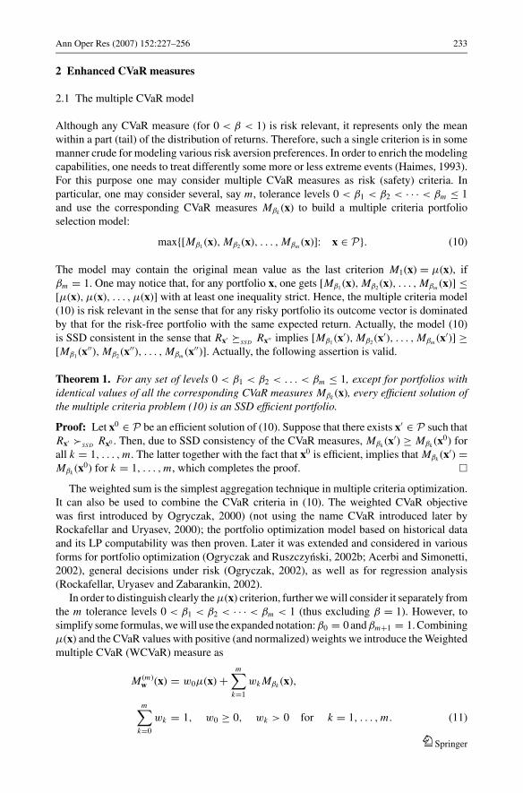
1

F(−2)x (p)

μ(x)

p

hβ(x)

β0

Mβ(x)

Δβ(x)

βμ(x)

F(−2)x (β)

12Γ(x)

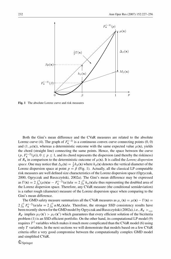
Fig. 1 The absolute Lorenz curve and risk measures

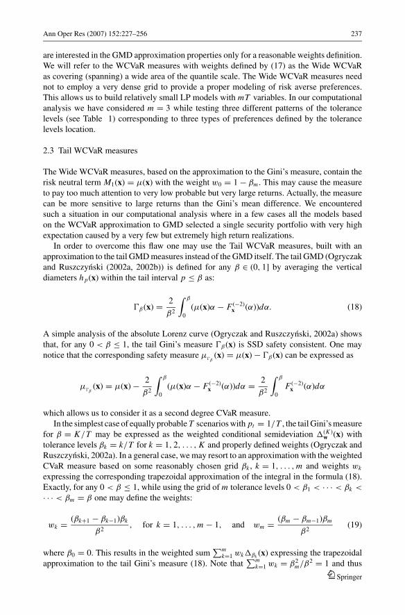
Both the Gini’s mean difference and the CVaR measures are related to the absolute

Lorenz curve (4). The graph of F (−2)x is a continuous convex curve connecting points (0, 0)

and (1, μ(x)), whereas a deterministic outcome with the same expected value μ(x), yields

the chord (straight line) connecting the same points. Hence, the space between the curve

(p, F (−2)x (p)), 0 ≤ p ≤ 1, and its chord represents the dispersion (and thereby the riskiness)

of Rx in comparison to the deterministic outcome of μ(x). It is called the Lorenz dispersionspace. One may notice that �β (x) = 1

βhβ (x) where hβ (x) denotes the vertical diameter of the

Lorenz dispersion space at point p = β (Fig. 1). Actually, all the classical LP computable

risk measures are well defined size characteristics of the Lorenz dispersion space (Ogryczak,

2000, Ogryczak and Ruszczynski, 2002a). The Gini’s mean difference may be expressed

as (x) = 2∫ 1

0(μ(x)α − F (−2)

x (α))dα = 2∫ 1

0hα(x)dα thus representing the doubled area of

the Lorenz dispersion space. Therefore, any CVaR measure (the conditional semideviation)

is a rather rough (diameter) measure of the Lorenz dispersion space when comparing to the

Gini’s mean difference.

The GMD safety measure summarizes all the CVaR measures as μ(x) = μ(x) − (x) =

2∫ 1

0F (−2)

x (α)dα = 2∫ 1

0αMα(x)dα. Therefore, the stronger SSD consistency results have

been recently shown for the GMD model by Ogryczak and Ruszczynski (2002a), i.e., Rx′ SSD

Rx′′ implies μ(x′) > μ(x′′) which guarantees that every efficient solution of the bicriteria

problem (1) is an SSD efficient portfolio. On the other hand, its computational LP model (9)

requires T 2 variables which makes it much more complicated than the CVaR model (6) using

only T variables. In the next sections we will demonstrate that models based on a few CVaR

criteria offer a very good compromise between the computationally complex GMD model

and simplified CVaR.

Springer

Ann Oper Res (2007) 152:227–256 233

2 Enhanced CVaR measures

2.1 The multiple CVaR model

Although any CVaR measure (for 0 < β < 1) is risk relevant, it represents only the mean

within a part (tail) of the distribution of returns. Therefore, such a single criterion is in some

manner crude for modeling various risk aversion preferences. In order to enrich the modeling

capabilities, one needs to treat differently some more or less extreme events (Haimes, 1993).

For this purpose one may consider multiple CVaR measures as risk (safety) criteria. In

particular, one may consider several, say m, tolerance levels 0 < β1 < β2 < · · · < βm ≤ 1

and use the corresponding CVaR measures Mβk (x) to build a multiple criteria portfolio

selection model:

max{[Mβ1(x), Mβ2

(x), . . . , Mβm (x)]: x ∈ P}. (10)

The model may contain the original mean value as the last criterion M1(x) = μ(x), if

βm = 1. One may notice that, for any portfolio x, one gets [Mβ1(x), Mβ2

(x), . . . , Mβm (x)] ≤[μ(x), μ(x), . . . , μ(x)] with at least one inequality strict. Hence, the multiple criteria model

(10) is risk relevant in the sense that for any risky portfolio its outcome vector is dominated

by that for the risk-free portfolio with the same expected return. Actually, the model (10)

is SSD consistent in the sense that Rx′ �SSD Rx′′ implies [Mβ1(x′), Mβ2

(x′), . . . , Mβm (x′)] ≥[Mβ1

(x′′), Mβ2(x′′), . . . , Mβm (x′′)]. Actually, the following assertion is valid.

Theorem 1. For any set of levels 0 < β1 < β2 < . . . < βm ≤ 1, except for portfolios withidentical values of all the corresponding CVaR measures Mβk (x), every efficient solution ofthe multiple criteria problem (10) is an SSD efficient portfolio.

Proof: Let x0 ∈ P be an efficient solution of (10). Suppose that there exists x′ ∈ P such that

Rx′ SSD Rx0 . Then, due to SSD consistency of the CVaR measures, Mβk (x′) ≥ Mβk (x0) for

all k = 1, . . . , m. The latter together with the fact that x0 is efficient, implies that Mβk (x′) =Mβk (x0) for k = 1, . . . , m, which completes the proof. �

The weighted sum is the simplest aggregation technique in multiple criteria optimization.

It can also be used to combine the CVaR criteria in (10). The weighted CVaR objective

was first introduced by Ogryczak, 2000) (not using the name CVaR introduced later by

Rockafellar and Uryasev, 2000); the portfolio optimization model based on historical data

and its LP computability was then proven. Later it was extended and considered in various

forms for portfolio optimization (Ogryczak and Ruszczynski, 2002b; Acerbi and Simonetti,

2002), general decisions under risk (Ogryczak, 2002), as well as for regression analysis

(Rockafellar, Uryasev and Zabarankin, 2002).

In order to distinguish clearly the μ(x) criterion, further we will consider it separately from

the m tolerance levels 0 < β1 < β2 < · · · < βm < 1 (thus excluding β = 1). However, to

simplify some formulas, we will use the expanded notation: β0 = 0 andβm+1 = 1. Combining

μ(x) and the CVaR values with positive (and normalized) weights we introduce the Weighted

multiple CVaR (WCVaR) measure as

M (m)w (x) = w0μ(x) +

m∑k=1

wk Mβk (x),

m∑k=0

wk = 1, w0 ≥ 0, wk > 0 for k = 1, . . . , m. (11)

Springer

234 Ann Oper Res (2007) 152:227–256

The WCVaR measure is a safety measure and it is risk relevant. The corresponding risk

measure turns out to be the weighted sum of the �βk (x) measures thus forming the weighted

conditional semideviation:

�(m)w (x) = μ(x) − M (m)

w (x) =m∑

k=1

wk�βk (x),m∑

k=1

wk ≤ 1, wk > 0 for k = 1, . . . , m.

(12)

The latter is not affected by any shift of the outcome scale and it is equal to 0 in the case of

a risk-free portfolio while taking positive value for any risky portfolio, thus representing a

translation invariant and risk relevant dispersion parameter. Therefore, we can consider the

corresponding Markowitz-type model and its mean-safety formalization (1):

max{[

μ(x), M (m)w (x)

]: x ∈ P

} = max{[

μ(x), μ(x) − �(m)w (x)

]: x ∈ P

}. (13)

Since the CVaR measures are coherent (Pflug, 2000) and SSD consistent (Ogryczak and

Ruszczynski, 2002a), the same applies to the WCVaR measure. In particular, Rx′ �SSD Rx′′

implies M (m)w (x′) ≥ M (m)

w (x′′) (Ogryczak and Ruszczynski, 2002b). Actually, the SSD consis-

tency relation for the WCVaR measure is stronger since it takes into account all the individual

CVaR measures as shown in the following assertion.

Theorem 2. For any set of levels 0 < β1 < β2 < · · · < βm ≤ 1, except for portfolios withidentical values of μ(x) and all conditional semideviations �βk (x), respectively, every efficientsolution of the bicriteria problem (13) is an SSD efficient portfolio.

Proof: Let x0 ∈ P be an efficient solution of (13). Suppose that there exists x′ ∈ P such

that Rx′ SSD Rx0 . Then, due to SSD consistency of the CVaR measures, μ(x′) ≥ μ(x0)

and Mβk (x′) ≥ Mβk (x0) for all k = 1, . . . , m. The latter, together with the fact that x0

is efficient, implies that μ(x′) = μ(x0) and∑m

k=1 wk Mβk (x′) = ∑mk=1 wk Mβk (x0). Hence,

Mβk (x′) = Mβk (x0) for k = 1, . . . , m, and therefore, �βk (x′) = �βk (x0) for all k = 1, . . . , m,

which completes the proof. �

For returns represented by their realizations we get an LP model. The model contains

the following core LP constraints to define a feasible portfolio, portfolio realizations, and

portfolio expected return:

x ∈ P, z ≥ μ0,

n∑j=1

μ j x j = z andn∑

j=1

r jt x j = yt for t = 1, . . . , T (14)

where z is an unbounded variable representing the mean return of the portfolio x and yt

(t = 1, . . . , T ) are unbounded variables to represent the realizations of the portfolio re-

turn under the scenario t . The general WCVaR model (13) leads us to the following LP

problem:

maximize w0z +m∑

k=1

wkqk −m∑

k=1

wk

βk

T∑t=1

pt dtk

subject to (14) and dtk − qk + yt ≥ 0, dtk ≥ 0 for t = 1, . . . , T ; k = 1, . . . , m(15)

Springer

Ann Oper Res (2007) 152:227–256 235

where qk (for k = 1, . . . , m) are unbounded variables taking the values of the corresponding

βk-quantiles (in the optimal solution). Except from the core constraints (14), model (15)

contains T nonnegative variables dtk and T corresponding linear inequalities for each k.

Thus, its dimensionality is proportional to the number of scenarios T and to the number of

tolerance levels m. Note that model (15) with m = 1 and w0 = 0 covers the standard CVaR

model, while m > 1 and various settings of positive weights wk allow us to model a wide

gamut of risk averse preferences. The model does not require any specific relation between

the number of scenarios T and the number of securities n or the number of tolerance levels m.

Similar to the Markowitz model, a very low number of scenarios may result in much less

diversified portfolios. Increasing the number of tolerance levels m, generally, enables a larger

diversification. However, such diversification is not guaranteed since, as demonstrated later,

it also depends on a specific weight-setting.

Recall that the absolute Lorenz curve, and thereby the CVaR measures, represent a

dual characterization of the SSD relation (Ogryczak and Ruszczynski, 2002a). Hence, the

weighted combination of the CVaR measures may be interpreted as the dual utility criterion

within the theory developed by Yaari (1987) which was recently reintroduced into the finance

literature in a simplified form of the spectral risk measures (Acerbi, 2002). Indeed, according

to (11),

M (m)w (x) = w0

∫ 1

0

F (−1)x (α)dα +

m∑k=1

wk

βk

∫ βk

0

F (−1)x (α)dα =

∫ 1

0

φ(α)F (−1)x (α)dα

where

φ(α) =

⎧⎪⎨⎪⎩w0 +m∑

k=i

wk

βk, βi−1 < α ≤ βi

w0, βm < α ≤ 1

(16)

is a decreasing risk aversion function (note the sign change for our safety measures to be

maximized).

As pointed out by Acerbi (2002), the subjective risk aversion of an investor can be encoded

in a function φ(α) defined for all possible confidence levels α ∈ (0, 1] and from a financial

point of view one cannot see any natural choice of function φ(α). The use of a wide class of risk

aversion functions in portfolio optimization (Acerbi and Simonetti, 2002) seems to be rather

far from the simplicity necessary to make possible an effective implementation of the portfo-

lio optimization procedure. In the following we will focus on the WCVaR measures defined

as simple combinations of a very few CVaR measures (thus stepwise risk aversion functions φ

with a very few steps). On the other hand, we introduce two specific types of weight-settings

which relate the WCVaR measure to the Gini’s mean difference and its tail version. This al-

lows us to use a few tolerance levels βk as the only parameters specifying the entire WCVaR

measures (modeling risk aversion function) while the corresponding weights are automati-

cally predefined by the requirements of the corresponding Gini’s measures. In other words, the

investor’s preferences are modeled by a selection of a few tolerance levels. It turns out that we

have managed to identify a class of simple WCVaR measures performing better in a real-life

portfolio optimization environment than typical CVaR measures and the GMD model.

2.2 Wide WCVaR measures

In the case of equally probable T scenarios with pt = 1/T (historical data for T periods),

the weighted CVaR measure M (T −1)w (x) defined with m = T − 1 tolerance levels βk = k/T

Springer

236 Ann Oper Res (2007) 152:227–256

for k = 1, 2, . . . , T − 1 represents the standard weighting approach in the multiple criteria

LP portfolio optimization model with criteria F (−2)(k/T ) (Ogryczak, 2000). The use of

weights wk = (2k)/T 2 for k = 1, 2, . . . , T − 1 and w0 = 1/T results then in �(T −1)w (x) =

2T

∑T −1k=1 h k

T(x) = (x) (c.f. Fig. 1). Hence, the WCVaR model is then equivalent to the GMD

model and it cannot provide us with any new modeling capabilities.

In the general case of T scenarios with arbitrary probabilities pt , one may use an ap-

proximation to (x) with �(m)w (x) based on some reasonably chosen grid of tolerance levels

βk , k = 1, . . . , m and weights wk expressing the corresponding trapezoidal approximation

to the integral formula (x) = 2∫ 1

0(μ(x)α − F (−2)

x (α))dα. Such an approximation is a very

attractive risk measure itself as it allows us to dramatically reduce the computational burden

caused by T 2 dimensionality of the LP implementation of the GMD model (9) while intro-

ducing new modeling capabilities connected to the grid selection. Exactly, for any grid of mtolerance levels 0 < β1 < · · · < βk < · · · < βm < 1 one gets the trapezoidal approximation:

(x) ∼=m∑

k=1

(βk+1 − βk−1)hβk (x) =m∑

k=1

(βk+1 − βk−1)βk�βk (x).

Note that∑m

k=1(βk+1 − βk−1)βk = βm < 1. This leads us to the WCVaR measure with

weights:

wk = (βk+1 − βk−1)βk, for k = 1, . . . , m, and w0 = 1 − βm . (17)

Precisely, when using the weights given by (17), the corresponding WCVaR measure defined

by (11) is an approximation to the GMD safety measure (8) (i.e., M (m)w (x) ∼= μ

(x)), and the

corresponding weighted conditional semideviation (12) is an approximation to the Gini’s

mean difference (x). This can be also illustrated in terms of the spectral measures (Acerbi,

2002) as integrating by parts one gets

μ(x) = 2

∫ 1

0

F (−2)x (α)dα = 2F (−2)

x (1) − 2

∫ 1

0

αF (−1)x (α)dα =

∫ 1

0

2(1 − α)F (−1)x (α)dα

which allows us to express the GMD safety measure by the risk aversion function φ(α) =2(1 − α) while formula (16) with the weights (17) defines a stepwise approximation to this

function.

Again, the WCVaR measures may be considered the exact GMD measure applied to (m +1)-point distributions approximating the original distribution of returns Rx, thus providing

a trapezoidal approximation to the original Lorenz dispersion space. In particular, for the

(m + 1)-point distribution Rx(β1 ,...,βm )

P{Rx(β1 ,...,βm ) = ξ} ={

βk − βk−1, ξ = ak for k = 1, . . . , m + 1

0, otherwise

such that a1 ≤ a2 ≤ · · · ≤ am+1, the weighted conditional semideviation �(m)w (x(β1,...,βm )) with

weights (17) is equal to (x(β1,...,βm )). In general, �(m)w (x) is a lower approximation to (x).

It must be emphasized that despite being only an approximation to the Gini’s mean

difference, any WCVaR measure with weights defined by (17) is a well defined LP computable

risk measure with guaranteed SSD consistency in the sense of Theorem 2. In other words, we

Springer

Ann Oper Res (2007) 152:227–256 237

are interested in the GMD approximation properties only for a reasonable weights definition.

We will refer to the WCVaR measures with weights defined by (17) as the Wide WCVaR

as covering (spanning) a wide area of the quantile scale. The Wide WCVaR measures need

not to employ a very dense grid to provide a proper modeling of risk averse preferences.

This allows us to build relatively small LP models with mT variables. In our computational

analysis we have considered m = 3 while testing three different patterns of the tolerance

levels (see Table 1) corresponding to three types of preferences defined by the tolerance

levels location.

2.3 Tail WCVaR measures

The Wide WCVaR measures, based on the approximation to the Gini’s measure, contain the

risk neutral term M1(x) = μ(x) with the weight w0 = 1 − βm . This may cause the measure

to pay too much attention to very low probable but very large returns. Actually, the measure

can be more sensitive to large returns than the Gini’s mean difference. We encountered

such a situation in our computational analysis where in a few cases all the models based

on the WCVaR approximation to GMD selected a single security portfolio with very high

expectation caused by a very few but extremely high return realizations.

In order to overcome this flaw one may use the Tail WCVaR measures, built with an

approximation to the tail GMD measures instead of the GMD itself. The tail GMD (Ogryczak

and Ruszczynski (2002a, 2002b)) is defined for any β ∈ (0, 1] by averaging the vertical

diameters h p(x) within the tail interval p ≤ β as:

β (x) = 2

β2

∫ β

0

(μ(x)α − F (−2)x (α))dα. (18)

A simple analysis of the absolute Lorenz curve (Ogryczak and Ruszczynski, 2002a) shows

that, for any 0 < β ≤ 1, the tail Gini’s measure β (x) is SSD safety consistent. One may

notice that the corresponding safety measure μβ

(x) = μ(x) − β (x) can be expressed as

μβ

(x) = μ(x) − 2

β2

∫ β

0

(μ(x)α − F (−2)x (α))dα = 2

β2

∫ β

0

F (−2)x (α)dα

which allows us to consider it as a second degree CVaR measure.

In the simplest case of equally probable T scenarios with pt = 1/T , the tail Gini’s measure

for β = K/T may be expressed as the weighted conditional semideviation �(K )w (x) with

tolerance levels βk = k/T for k = 1, 2, . . . , K and properly defined weights (Ogryczak and

Ruszczynski, 2002a). In a general case, we may resort to an approximation with the weighted

CVaR measure based on some reasonably chosen grid βk , k = 1, . . . , m and weights wk

expressing the corresponding trapezoidal approximation of the integral in the formula (18).

Exactly, for any 0 < β ≤ 1, while using the grid of m tolerance levels 0 < β1 < · · · < βk <

· · · < βm = β one may define the weights:

wk = (βk+1 − βk−1)βk

β2, for k = 1, . . . , m − 1, and wm = (βm − βm−1)βm

β2(19)

where β0 = 0. This results in the weighted sum∑m

k=1 wk�βk (x) expressing the trapezoidal

approximation to the tail Gini’s measure (18). Note that∑m

k=1 wk = β2m/β2 = 1 and thus

Springer

238 Ann Oper Res (2007) 152:227–256

we get a regular weighted conditional semideviation (12) �(m)w (x) ∼= β (x). Further, weights

(19) together with w0 = 0 generate a WCVaR measure (11) such that M (m)w (x) ∼= μ

β(x).

This can also be illustrated in terms of the spectral measures (Acerbi, 2002) as integrating

by parts one gets

μβ

(x) = 2

β2

∫ β

0

F (−2)x (α)dα = 2

βF (−2)

x (β)

− 2

β2

∫ β

0

αF (−1)x (α)dα =

∫ 1

0

2(β − α)+

β2F (−1)

x (α)dα

allowing us to express the tail GMD safety measure by the risk aversion function φ(α) =2(β − α)+/β2 where (.)+ denotes the nonnegative part of a number. Formula (16) with the

weights (19) defines a stepwise approximation to this function.

Again, we emphasize that despite being only an approximation to (18), any Tail WCVaR

measure (e.g., a WCVaR measure with weights defined according to (19)) is a well defined

LP computable measure with guaranteed SSD consistency in the sense of Theorem 2. They

need not be built on a very dense grid to provide proper modeling of risk averse preferences.

Actually, we are interested in a direct preference modeling with simple Tail WCVaR measures

rather than strict approximation to the Tail GMD measure. In our computational analysis we

have tested two Tail WCVaR models with m = 2 and m = 3 (see Table 1). Obviously, all the

Tail WCVaR model measures are implemented as LP problems (15) but with w0 = 0. Again,

for a small value of m we get rather small LP models with mT variables.

2.4 Direct diversification enforcement

Since the seminal work of Markowitz (1952), the notion of investing in diversified portfolios

is considered one of the most fundamental concepts of portfolio management. Diversification

should be enforced by the mean/risk preference model. Indeed, in the original Markowitz

model it was usually guaranteed by the standard deviation (variance) minimization. In gen-

eral, it may happen that a single security or a low diversified portfolio is SSD dominating over

all other (more diversified) portfolios, and the SSD consistent Markowitz-type models will

select such an undiversified solution. Especially, the SSD consistent models based on the LP

computable risk measures may fail to generate sufficiently diversified portfolios, although this

also happens for the original Markowitz model (Mansini, Ogryczak and Speranza, 2003b).

Therefore, additional restrictions may be posed on the feasible portfolios to guarantee the

required diversification. The simplest way to enforce portfolio diversification is to limit the

maximum share. This, however, allows us to form a portfolio with a few shares at the max-

imum level. A better modeling alternative would be to allow for a relatively large maximum

share provided that the other shares are smaller. Such a rich diversification scheme may be

introduced with the CVaR constructs applied to the right tail of the distribution of shares.

A natural generalization of the maximum share is the (right-tail) conditional mean de-

fined as the mean within the specified tolerance level (amount) of the worst shares. One

may simply define the conditional mean as the mean of the k largest shares. This can

be formalized as follows. First, we introduce the ordering map � : Rn → Rn such that

�(x) = (θ1(x), θ2(x), . . . , θn(x)), where θ1(x) ≥ θ2(x) ≥ · · · ≥ θn(x) and there exists a per-

mutation τ of set J such that θ j (x) = xτ ( j) for j = 1, . . . , n. The use of ordered outcome

vectors �(x) allows us to focus on distributions of shares impartially. Next, the linear cu-

mulative map is applied to ordered vectors to get θk(x) = ∑kj=1 θ j (x) for k = 1, . . . , n. The

Springer

Ann Oper Res (2007) 152:227–256 239

coefficients of vector �(x) = (θ1(x), θ2(x), . . . , θn(x)) express, respectively: the largest share,

the total of the two largest shares, the total of the three largest shares, etc. Hence, the (worst)kn –conditional mean share is given as 1

k θk(x), for k = 1, . . . , n.

Similar to the CVaR formulas, for a given vector x, the value of θk(x) may be found by

solving the linear program (Ogryczak and Tamir, 2003):

θk(x) = min

{ksk +

n∑j=1

dsk j : ds

k j ≥ x j − sk, dsk j ≥ 0 for j = 1, . . . , n

},

where sk is an unbounded variable (representing the k-th largest share at the optimum) and

dsk j are additional nonnegative (deviational) variables. Hence, any model under consideration

can easily be extended with direct diversification constraints specified as θk(x) ≤ ck upper

bounding total of the k largest shares and implemented with linear inequalities:

ksk +n∑

j=1

dsk j ≤ ck and ds

k j ≥ x j − sk, dsk j ≥ 0 for j = 1, . . . , n. (20)

3 Experimental analysis

3.1 Testing environment

The present section is devoted to the experimental analysis in a real framework of all the

described LP models based on extensions of the CVaR measure. Models have been tested on

a PC with a 500 MHz Pentium processor by using CPLEX 6.5 package. First we present the

test problems. Then the results of the in-sample analysis, both on the original models and on

their modifications to enforce diversification, are described. Next, the out-of-sample analy-

sis including the results obtained through the simulation of a “multiperiod-type” portfolio

investment is presented. Finally, portfolio performances in a separated period characterized

by a strong drawdown trend are discussed.

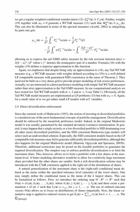
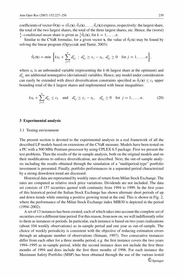
Historical data are represented by weekly rates of return from Milan Stock Exchange. The

rates are computed as relative stock price variations. Dividends are not included. The data

set consists of 157 securities quoted with continuity from 1994 to 1999. In the first years

of this historical period the Italian Stock Exchange has shown alternate short periods of up

and down trends while entering a positive growing trend at the end. This is shown in Fig. 2,

where the performance of the Milan Stock Exchange index MIB30 is depicted in the period

(1994–2002).

A set of 13 instances has been created, each of which takes into account the complete set of

securities over a different time period. For this reason, from now on, we will indifferently refer

to them as instances or periods. In particular, each instance is based on two years realizations

(about 104 weekly observations) as in-sample period and one year as out-of-sample. The

choice of weekly periodicity is consistent with the objective of reducing estimation errors

through an adequate number of observations (Simaan, 1997). Two consecutive instances

differ from each other for a three months period, e.g. the first instance covers the two years

1994–1995 as in-sample period, while the second instance does not include the first three

months of 1994 and does include the first three months of 1996. For each instance the

Maximum Safety Portfolio (MSP) has been obtained through the use of the various tested

Springer

240 Ann Oper Res (2007) 152:227–256

Fig. 2 The Milan Stock Exchange Index MIB30: weekly quotations in the years 1994–2002 (source: DATAS-TREAM)

models. In this section we only summarize and comment the main figures out of the huge

amount of computational results we obtained.

The model introduced by Young (1998), with safety measure the maximization of the

worst realization (7), is identified as Minimax. The model based on the safety measure

corresponding to the Gini’s mean difference (9), i.e. the mean worse return, is referred simply

as GMD. The CVaR model associated to a given tolerance level β is identified as CVaR(β).

We have tested the CVaR model for five different values of β, i.e. CVaR(0.05), CVaR(0.1),

CVaR(0.25), CVaR(0.5) and CVaR(0.75). All the CVaR and the weighted CVaR models have

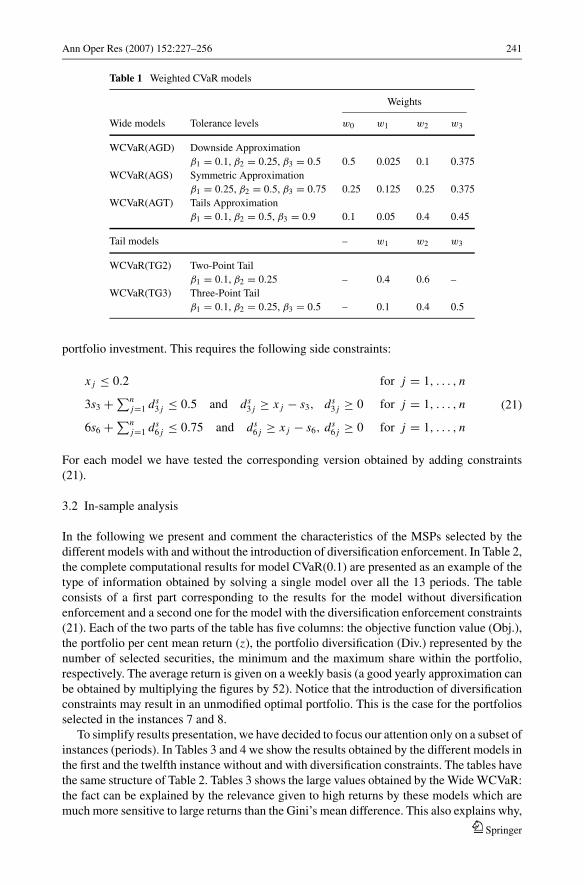
been formulated according to (15). Among the weighted models we have tested three Wide

WCVaR models (with m = 3 tolerance levels) and two Tail WCVaR models (with m = 2

and m = 3, respectively). The corresponding tolerance levels and weights are summarized

in Table 1.

Since SSD consistent models based on the LP computable risk measures may fail to

generate diversified enough portfolios we have added the following additional restrictions

to guarantee sufficient diversification: any stock share cannot exceed 0.20, while any three

shares cannot exceed 0.50 in total and any six shares cannot globally exceed 0.75 of the

Springer

Ann Oper Res (2007) 152:227–256 241

Table 1 Weighted CVaR models

Weights

Wide models Tolerance levels w0 w1 w2 w3

WCVaR(AGD) Downside Approximation

β1 = 0.1, β2 = 0.25, β3 = 0.5 0.5 0.025 0.1 0.375

WCVaR(AGS) Symmetric Approximation

β1 = 0.25, β2 = 0.5, β3 = 0.75 0.25 0.125 0.25 0.375

WCVaR(AGT) Tails Approximation

β1 = 0.1, β2 = 0.5, β3 = 0.9 0.1 0.05 0.4 0.45

Tail models – w1 w2 w3

WCVaR(TG2) Two-Point Tail

β1 = 0.1, β2 = 0.25 – 0.4 0.6 –

WCVaR(TG3) Three-Point Tail

β1 = 0.1, β2 = 0.25, β3 = 0.5 – 0.1 0.4 0.5

portfolio investment. This requires the following side constraints:

x j ≤ 0.2 for j = 1, . . . , n

3s3 + ∑nj=1 ds

3 j ≤ 0.5 and ds3 j ≥ x j − s3, ds

3 j ≥ 0 for j = 1, . . . , n

6s6 + ∑nj=1 ds

6 j ≤ 0.75 and ds6 j ≥ x j − s6, ds

6 j ≥ 0 for j = 1, . . . , n

(21)

For each model we have tested the corresponding version obtained by adding constraints

(21).

3.2 In-sample analysis

In the following we present and comment the characteristics of the MSPs selected by the

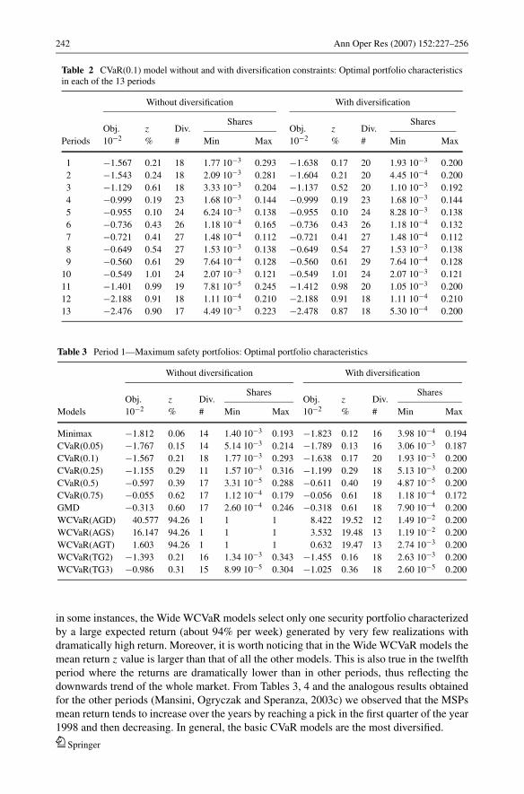
different models with and without the introduction of diversification enforcement. In Table 2,

the complete computational results for model CVaR(0.1) are presented as an example of the

type of information obtained by solving a single model over all the 13 periods. The table

consists of a first part corresponding to the results for the model without diversification

enforcement and a second one for the model with the diversification enforcement constraints

(21). Each of the two parts of the table has five columns: the objective function value (Obj.),

the portfolio per cent mean return (z), the portfolio diversification (Div.) represented by the

number of selected securities, the minimum and the maximum share within the portfolio,

respectively. The average return is given on a weekly basis (a good yearly approximation can

be obtained by multiplying the figures by 52). Notice that the introduction of diversification

constraints may result in an unmodified optimal portfolio. This is the case for the portfolios

selected in the instances 7 and 8.

To simplify results presentation, we have decided to focus our attention only on a subset of

instances (periods). In Tables 3 and 4 we show the results obtained by the different models in

the first and the twelfth instance without and with diversification constraints. The tables have

the same structure of Table 2. Tables 3 shows the large values obtained by the Wide WCVaR:

the fact can be explained by the relevance given to high returns by these models which are

much more sensitive to large returns than the Gini’s mean difference. This also explains why,

Springer

242 Ann Oper Res (2007) 152:227–256

Table 2 CVaR(0.1) model without and with diversification constraints: Optimal portfolio characteristicsin each of the 13 periods

Without diversification With diversification

Shares SharesObj. z Div. Obj. z Div.

Periods 10−2 % # Min Max 10−2 % # Min Max

1 −1.567 0.21 18 1.77 10−3 0.293 −1.638 0.17 20 1.93 10−3 0.200

2 −1.543 0.24 18 2.09 10−3 0.281 −1.604 0.21 20 4.45 10−4 0.200

3 −1.129 0.61 18 3.33 10−3 0.204 −1.137 0.52 20 1.10 10−3 0.192

4 −0.999 0.19 23 1.68 10−3 0.144 −0.999 0.19 23 1.68 10−3 0.144

5 −0.955 0.10 24 6.24 10−3 0.138 −0.955 0.10 24 8.28 10−3 0.138

6 −0.736 0.43 26 1.18 10−4 0.165 −0.736 0.43 26 1.18 10−4 0.132

7 −0.721 0.41 27 1.48 10−4 0.112 −0.721 0.41 27 1.48 10−4 0.112

8 −0.649 0.54 27 1.53 10−3 0.138 −0.649 0.54 27 1.53 10−3 0.138

9 −0.560 0.61 29 7.64 10−4 0.128 −0.560 0.61 29 7.64 10−4 0.128

10 −0.549 1.01 24 2.07 10−3 0.121 −0.549 1.01 24 2.07 10−3 0.121

11 −1.401 0.99 19 7.81 10−5 0.245 −1.412 0.98 20 1.05 10−3 0.200

12 −2.188 0.91 18 1.11 10−4 0.210 −2.188 0.91 18 1.11 10−4 0.210

13 −2.476 0.90 17 4.49 10−3 0.223 −2.478 0.87 18 5.30 10−4 0.200

Table 3 Period 1—Maximum safety portfolios: Optimal portfolio characteristics

Without diversification With diversification

Shares SharesObj. z Div. Obj. z Div.

Models 10−2 % # Min Max 10−2 % # Min Max

Minimax −1.812 0.06 14 1.40 10−3 0.193 −1.823 0.12 16 3.98 10−4 0.194

CVaR(0.05) −1.767 0.15 14 5.14 10−3 0.214 −1.789 0.13 16 3.06 10−3 0.187

CVaR(0.1) −1.567 0.21 18 1.77 10−3 0.293 −1.638 0.17 20 1.93 10−3 0.200

CVaR(0.25) −1.155 0.29 11 1.57 10−3 0.316 −1.199 0.29 18 5.13 10−3 0.200

CVaR(0.5) −0.597 0.39 17 3.31 10−5 0.288 −0.611 0.40 19 4.87 10−5 0.200

CVaR(0.75) −0.055 0.62 17 1.12 10−4 0.179 −0.056 0.61 18 1.18 10−4 0.172

GMD −0.313 0.60 17 2.60 10−4 0.246 −0.318 0.61 18 7.90 10−4 0.200

WCVaR(AGD) 40.577 94.26 1 1 1 8.422 19.52 12 1.49 10−2 0.200

WCVaR(AGS) 16.147 94.26 1 1 1 3.532 19.48 13 1.19 10−2 0.200

WCVaR(AGT) 1.603 94.26 1 1 1 0.632 19.47 13 2.74 10−3 0.200

WCVaR(TG2) −1.393 0.21 16 1.34 10−3 0.343 −1.455 0.16 18 2.63 10−3 0.200

WCVaR(TG3) −0.986 0.31 15 8.99 10−5 0.304 −1.025 0.36 18 2.60 10−5 0.200

in some instances, the Wide WCVaR models select only one security portfolio characterized

by a large expected return (about 94% per week) generated by very few realizations with

dramatically high return. Moreover, it is worth noticing that in the Wide WCVaR models the

mean return z value is larger than that of all the other models. This is also true in the twelfth

period where the returns are dramatically lower than in other periods, thus reflecting the

downwards trend of the whole market. From Tables 3, 4 and the analogous results obtained

for the other periods (Mansini, Ogryczak and Speranza, 2003c) we observed that the MSPs

mean return tends to increase over the years by reaching a pick in the first quarter of the year

1998 and then decreasing. In general, the basic CVaR models are the most diversified.

Springer

Ann Oper Res (2007) 152:227–256 243

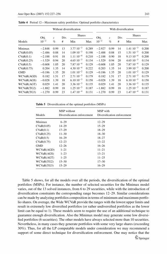
Table 4 Period 12—Maximum safety portfolios: Optimal portfolio characteristics

Without diversification With diversification

Shares SharesObj. z Div. Obj. z Div.

Models 10−2 % # Min Max 10−2 % # Min Max

Minimax −2.848 0.99 13 3.77 10−3 0.289 −2.927 0.99 14 1.41 10−3 0.200

CVaR(0.05) −2.486 0.88 14 1.09 10−3 0.198 −2.488 0.88 15 1.51 10−3 0.200

CVaR(0.1) −2.188 0.91 18 1.11 10−4 0.210 −2.188 0.90 18 9.13 10−4 0.200

CVaR(0.25) −1.529 0.94 20 4.65 10−3 0.134 −1.529 0.94 20 4.65 10−3 0.134

CVaR(0.5) −0.608 1.05 20 7.87 10−4 0.129 −0.608 1.05 20 7.87 10−4 0.129

CVaR(0.75) 0.204 1.35 14 4.30 10−4 0.222 0.203 1.35 14 3.99 10−3 0.200

GMD −0.186 1.35 20 1.01 10−2 0.129 −0.186 1.35 20 1.01 10−2 0.129

WCVaR(AGD) 0.182 1.51 17 2.71 10−3 0.179 0.182 1.51 17 2.71 10−3 0.179

WCVaR(AGS) −0.028 1.39 18 6.10 10−3 0.158 −0.028 1.39 18 6.10 10−3 0.158

WCVaR(AGT) 0.029 1.41 20 3.36 10−3 0.135 0.029 1.41 20 3.36 10−3 0.135

WCVaR(TG2) −1.882 0.99 18 1.25 10−3 0.187 −1.882 0.99 18 1.25 10−3 0.187

WCVaR(TG3) −1.270 0.99 23 1.47 10−4 0.131 −1.270 0.99 23 1.47 10−4 0.131

Table 5 Diversification of the optimal portfolios (MSPs)

MSP without MSP with

Models Diversification enforcement Diversification enforcement

Minimax 6–29 12–29

CVaR(0.05) 14–29 15–29

CVaR(0.1) 17–29 18–29

CVaR(0.25) 11–30 18–30

CVaR(0.5) 16–29 18–27

CVaR(0.75) 12–23 13–22

GMD 12–26 16–26

WCVaR(AGD) 1–21 11–21

WCVaR(AGS) 1–23 13–21

WCVaR(AGT) 1–25 11–25

WCVaR(TG2) 15–30 17–30

WCVaR(TG3) 15–29 16–29

Table 5 shows, for all the models over all the periods, the diversification of the optimal

portfolios (MSPs). For instance, the number of selected securities for the Minimax model

varies, out of the 13 solved instances, from 6 to 29 securities, while with the introduction of

diversification constraints the corresponding range becomes 12–29. Similar considerations

can be made by analyzing portfolios composition in terms of minimum and maximum portfo-

lio shares. On average, the Wide WCVaR provide the ranges with the lowest upper limits and

result in extremely low diversified portfolios (or rather undiversified portfolios as the lower

limit can be equal to 1). These models seem to require the use of an additional technique to

guarantee enough diversification. Also the Minimax model may generate some low diversi-

fied portfolios (6 securities). The other models have always selected more than 10 securities.

Nevertheless, in many cases they generate portfolios with some very large shares (exceeding

30%). Thus, for all the LP computable models under consideration we may recommend a

support of some direct technique for diversification enforcement. One may notice that the

Springer

244 Ann Oper Res (2007) 152:227–256

application of the CVaR based diversification enforcement constraints (21) has resulted in

portfolios always containing at least 10 securities.

3.3 Out-of-sample analysis

In this section the behavior of all the MSPs is examined in the twelve months following the date

of each portfolio selection. To describe out-of-sample results we have used the following nine

ex-post parameters: the minimum, the average, the maximum and the median portfolio return

(rmin, rav, rmax and rmed, respectively); the standard deviation (std) and the semi-standard

deviation (s-std); the mean absolute deviation (MAD) and the mean downside semideviation

(s-MAD); the maximum downside deviation (D-DEV). Such performance criteria have been

computed for all the models over all the periods and can be used to compare the out-of-sample

behavior of the maximum safety portfolios selected by the different models. The minimum,

average, maximum and median ex-post portfolio returns are expressed on a yearly basis. All

the dispersion measures (std, s-std, MAD, s-MAD and D-DEV) have been computed with

respect to the target return μ0 (which is zero for the MSP) to make them directly comparable

in the different models.

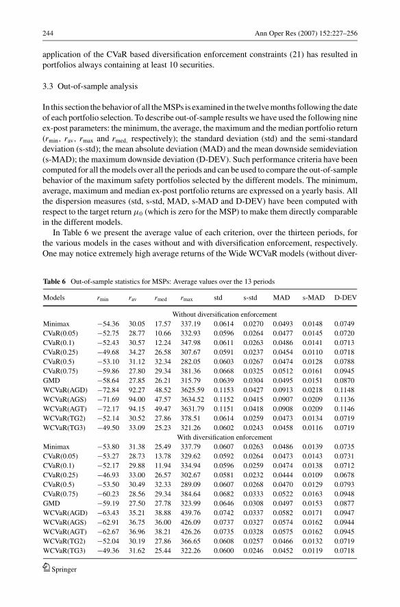
In Table 6 we present the average value of each criterion, over the thirteen periods, for

the various models in the cases without and with diversification enforcement, respectively.

One may notice extremely high average returns of the Wide WCVaR models (without diver-

Table 6 Out-of-sample statistics for MSPs: Average values over the 13 periods

Models rmin rav rmed rmax std s-std MAD s-MAD D-DEV

Without diversification enforcement

Minimax −54.36 30.05 17.57 337.19 0.0614 0.0270 0.0493 0.0148 0.0749

CVaR(0.05) −52.75 28.77 10.66 332.93 0.0596 0.0264 0.0477 0.0145 0.0720

CVaR(0.1) −52.43 30.57 12.24 347.98 0.0611 0.0263 0.0486 0.0141 0.0713

CVaR(0.25) −49.68 34.27 26.58 307.67 0.0591 0.0237 0.0454 0.0110 0.0718

CVaR(0.5) −53.10 31.12 32.34 282.05 0.0603 0.0267 0.0474 0.0128 0.0788

CVaR(0.75) −59.86 27.80 29.34 381.36 0.0668 0.0325 0.0512 0.0161 0.0945

GMD −58.64 27.85 26.21 315.79 0.0639 0.0304 0.0495 0.0151 0.0870

WCVaR(AGD) −72.84 92.27 48.52 3625.59 0.1153 0.0427 0.0913 0.0218 0.1148

WCVaR(AGS) −71.69 94.00 47.57 3634.52 0.1152 0.0415 0.0907 0.0209 0.1136

WCVaR(AGT) −72.17 94.15 49.47 3631.79 0.1151 0.0418 0.0908 0.0209 0.1146

WCVaR(TG2) −52.14 30.52 27.86 378.51 0.0614 0.0259 0.0473 0.0134 0.0719

WCVaR(TG3) −49.50 33.09 25.23 321.26 0.0602 0.0243 0.0458 0.0116 0.0719

With diversification enforcement

Minimax −53.80 31.38 25.49 337.79 0.0607 0.0263 0.0486 0.0139 0.0735

CVaR(0.05) −53.27 28.73 13.78 329.62 0.0592 0.0264 0.0473 0.0143 0.0731

CVaR(0.1) −52.17 29.88 11.94 334.94 0.0596 0.0259 0.0474 0.0138 0.0712

CVaR(0.25) −46.93 33.00 26.57 302.67 0.0581 0.0232 0.0444 0.0109 0.0678

CVaR(0.5) −53.50 30.49 32.33 289.09 0.0607 0.0268 0.0470 0.0129 0.0793

CVaR(0.75) −60.23 28.56 29.34 384.64 0.0682 0.0333 0.0522 0.0163 0.0948

GMD −59.19 27.50 27.78 323.99 0.0646 0.0308 0.0497 0.0153 0.0877

WCVaR(AGD) −63.43 35.21 38.88 439.76 0.0742 0.0337 0.0582 0.0171 0.0947

WCVaR(AGS) −62.91 36.75 36.00 426.09 0.0737 0.0327 0.0574 0.0162 0.0944

WCVaR(AGT) −62.67 36.96 38.21 426.26 0.0735 0.0328 0.0575 0.0162 0.0945

WCVaR(TG2) −52.04 30.19 27.86 366.65 0.0608 0.0257 0.0466 0.0132 0.0719

WCVaR(TG3) −49.36 31.62 25.44 322.26 0.0600 0.0246 0.0452 0.0119 0.0718

Springer

Ann Oper Res (2007) 152:227–256 245

sification enforcement). These performances are produced by single security portfolios with

very high returns. In general, the models are too risky as demonstrated by all the dispersion

measures. When we consider the models with diversification enforcement, the Wide WC-

VaR models are still characterized by the highest average returns and the largest dispersion

parameters but the differences from the other models are not very large. One may notice that

the GMD model, which is the computationally most complex, may be easily outperformed

(in terms of average returns and dispersion) by the simpler Tail WCVaR models or even by

CVaR(0.5).

We have also analyzed each model performance with respect to a long-run portfolio

management. Each of the portfolios selected by a specific model in the 13 instances has been

evaluated ex-post in the three months period following the date of selection. It turned out that

single period ex-post returns quite perfectly represent the upward and downward movements

of the market. For instance, all the models showed negative results from April to July 1996

and then again in October when the market was falling down. However, in such periods

some models (such as CVaR(0.1) and CVaR(0.25)) find portfolios with a better performance

with respect to the market index MIB30. Similarly, many models find higher returns with

respect to the MIB30 index at the beginning of the 1998 when the market showed a positive

trend (see Fig. 2). Full results of this analysis can be found in our technical report (Mansini,

Ogryczak and Speranza, 2003c). Further, we cumulated the returns over the horizon up to

13 periods (39 months) to better analyze each model achievements. The figures shown in

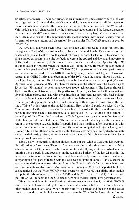
Table 7 are the cumulative returns of the portfolios selected by each model in the case without

diversification enforcement and with diversification enforcement, respectively. Each column

of these tables refers to a period and provides the cumulative returns of the portfolios selected

over the preceding periods. For a better understanding of these figures let us consider the first

line of Table 7 which refers to the model Minimax. Each of the 13 portfolios selected by the

Minimax model in the 13 instances has been evaluated ex-post in the three months investment

period following the date of its selection. Let us define as r1, r2, . . . , r13 the ex-post returns of

these 13 portfolios. Then, the first column of Table 7 gives the ex-post return (after 3 months)

of the first portfolio selected, i.e. r1. The second column of Table 7 gives the cumulative

return of the portfolio selected in the first period and then modified after three months with

the portfolio selected in the second period: the value is computed as (1 + r1)(1 + r2) − 1.

Similarly, for all the other columns of the table. These results have been computed to simulate

a multi-period setting where, at no transaction cost, the portfolio changes over time. Rates

are expressed on a yearly basis.

Table 7 shows extremely high cumulative returns of the Wide WCVaR models (without

diversification enforcement). These performances are due to the single security portfolios

selected in the first 6 periods which resulted in dramatically high returns. Actually, when

ignoring these 6 periods and focusing on the remaining horizon of the last 21 months, the

cumulative returns of the Wide WCVaR models considerably shrink as it is evident when

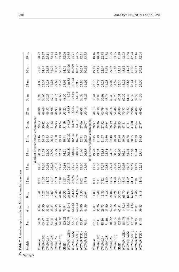
comparing the first part of Table 8 with the last seven columns of Table 7. Table 8 shows the

ex-post cumulative returns over the last 21 months (7 periods) both for the case without and

with diversification enforcement. Moreover, as in column (7–13) of the first part of Table 8, it

can be noticed that the Wide WCVaR models perform much worse than all the other models

except for the Minimax and the extremal CVaR models (β = 0.05 or β = 0.1). Note that both

the Tail WCVaR models and the CVaR(0.5) here have the best cumulative performances.

When the models with diversification enforcement are considered, the Wide WCVaR

models are still characterized by the highest cumulative returns but the differences from the

other models are not very large. When ignoring the first 6 periods and focusing on the last 21

months (second part of Table 8), one may see again the Wide WCVaR models performing

Springer

246 Ann Oper Res (2007) 152:227–256

Tabl

e7

Ou

t-o

f-sa

mp

lere

sult

sfo

rM

SP

s:C

um

ula

tive

retu

rns

Mo

del

s3

m.

6m

.9

m.

12

m.

15

m.

18

m.

21

m.

24

m.

27

m.

30

m.

33

m.

36

m.

39

m.

Wit

ho

ut

div

ersi

fica

tio

nen

forc

emen

t

Min

imax

54

.09

32

.04

13

.41

9.2

31

8.2

02

0.5

92

3.1

62

9.6

34

8.8

03

8.9

72

4.0

02

1.9

02

0.9

7

CV

aR(0

.05

)6

3.8

73

5.3

01

5.2

71

0.5

71

9.3

62

1.5

82

4.0

33

0.4

24

9.6

03

9.6

52

7.3

32

4.4

92

3.2

7

CV

aR(0

.1)

64

.54

35

.63

17

.87

11

.72

20

.91

22

.00

24

.33

30

.04

49

.37

39

.25

27

.28

23

.95

25

.11

CV

aR(0

.25

)7

3.0

53

4.3

31

9.6

71

4.3

02

5.2

32

7.3

92

6.3

33

1.2

25

1.9

84

7.1

93

2.2

53

2.2

23

2.4

3

CV

aR(0

.5)

96

.96

54

.35

23

.46

15

.71

22

.35

25

.29

23

.00

26

.93

48

.93

44

.15

29

.62

30

.43

32

.43

CV

aR(0

.75

)1

48

.85

81

.32

41

.84

23

.07

29

.40

32

.38

29

.23

30

.24

54

.89

48

.60

32

.46

36

.35

33

.60

GM

D1

28

.21

71

.94

36

.35

19

.84

26

.98

34

.21

30

.41

31

.19

53

.25

48

.36

33

.61

34

.71

32

.66

WC

VaR

(AG

D)

32

2.7

36

47

.41

26

4.6

72

05

.56

21

3.2

12

08

.53

16

7.2

21

46

.28

16

8.8

51

44

.28

11

0.5

21

03

.96

94

.55

WC

VaR

(AG

S)

32

2.7

36

47

.41

26

4.6

72

05

.56

21

3.2

12

08

.53

16

5.3

21

44

.96

16

7.4

91

42

.49

10

7.7

41

02

.99

93

.71

WC

VaR

(AG

T)

32

2.7

36

47

.41

26

4.6

72

05

.56

21

3.2

12

08

.53

16

7.2

11

44

.12

16

7.3

81

44

.33

10

9.7

11

02

.87

94

.55

WC

VaR

(TG

2)

53

.17

24

.90

11

.50

8.0

21

9.8

02

1.4

62

2.4

12

7.6

64

8.0

83

9.5

92

7.8

02

6.2

73

2.7

1

WC

VaR

(TG

3)

78

.91

41

.59

20

.94

13

.41

23

.99

26

.85

26

.05

29

.07

50

.19

45

.29

31

.02

30

.92

33

.35

Wit

hd

iver

sifi

cati

on

enfo

rcem

ent

Min

imax

67

.81

37

.87

11

.83

8.1

31

7.2

51

9.7

82

2.4

52

8.9

74

8.1

33

8.4

12

3.1

61

9.8

71

8.1

6

CV

aR(0

.05

)5

7.1

13

5.2

61

0.4

27

.11

16

.36

19

.03

21

.79

28

.36

47

.50

37

.88

24

.77

22

.18

20

.88

CV

aR(0

.1)

48

.16

28

.73

11

.86

7.4

21

7.1

71

8.8

52

1.5

72

7.5

24

6.7

93

7.0

82

5.2

32

2.0

92

2.3

8

CV

aR(0

.25

)7

1.1

03

3.5

01

5.8

61

1.5

62

2.8

22

5.3

42

4.5

92

9.6

45

0.3

54

5.7

63

1.2

53

1.3

13

1.5

8

CV

aR(0

.5)

10

0.5

55

2.2

22

1.8

41

4.3

72

1.2

12

4.3

22

2.1

82

6.1

94

8.1

64

3.4

82

9.0

72

9.9

33

1.9

5

CV

aR(0

.75

)1

45

.52

78

.16

40

.21

21

.44

27

.98

30

.95

28

.78

29

.84

54

.46

48

.23

31

.59

35

.63

33

.35

GM

D1

27

.84

65

.51

30

.75

15

.54

23

.25

30

.90

27

.84

28

.93

50

.90

46

.31

32

.10

33

.31

31

.39

WC

VaR

(AG

D)

18

4.7

81

43

.24

65

.70

43

.49

50

.95

56

.21

49

.09

47

.81

70

.77

62

.37

45

.22

45

.12

42

.03

WC

VaR

(AG

S)

17

0.4

91

32

.87

61

.94

41

.25

49

.33

55

.95

48

.38

47

.31

70

.22

61

.44

43

.65

44

.75

41

.88

WC

VaR

(AG

T)

17

3.3

61

34

.87

62

.66

41

.11

50

.59

57

.68

50

.35

47

.60

70

.96

63

.37

45

.44

45

.06

42

.74

WC

VaR

(TG

2)

50

.35

27

.01

11

.46

7.9

91

9.7

82

1.4

42

2.3

92

7.6

44

8.0

63

9.5

82

7.7

52

6.2

33

2.1

6

WC

VaR

(TG

3)

81

.68

39

.85

18

.18

11

.49

22

.31

25

.41

24

.83

27

.97

49

.05

44

.30

29

.50

29

.52

32

.04

Springer

Ann Oper Res (2007) 152:227–256 247

Tabl

e8

Ou

t-o

f-sa

mp

leco

mp

uta

tio

nal

resu

lts:

Cu

mu

lati

ve

retu

rns

over

the

late

st2

1m

on

ths

(7p

erio

ds)

Wit

ho

ut

div

ersi

fica

tio

nW

ith

div

ersi

fica

tio

nP

erio

ds

Mo

del

s7

7–

87

–9

7–

10

7–

11

7–

12

7–

13

77

–8

7–

97

–1

07

–1

17

–1

27

–1

3

Min

imax

39

.77

60

.99

11

5.2

47

1.9

12

8.2

32

3.2

22

2.8

33

9.7

76

0.9

91

15

.24

71

.91

27

.35

19

.96

16

.79

CV

aR(0

05

)3

9.7

76

0.9

91

15

.24

71

.91

34

.59

27

.47

24

.74

39

.77

60

.99

11

5.2

47

1.9

13

2.0

22

5.4

22

2.4

9

CV

aR(0

1)

39

.23

57

.50

11

2.9

26

9.8

13

3.9

32

5.9

32

7.8

43

9.2

35

7.5

01

12

.92

69

.81

33

.34

25

.42

25

.48

CV

aR(0

25

)2

0.1

64

3.4

41

06

.15

8.2

83

8.3

23

7.2

43

6.9

02

0.1

64

3.4

41

06

.15

8.2

83

8.7

03

7.5

53

7.1

7

CV

aR(0

5)

10

.14

32

.00

10

0.8

77

7.9

13

5.0

23

5.7

93

8.8

81

0.1

43

2.0

01

00

.87

77

.91

35

.02

35

.79

38

.88

CV

aR(0

75

)1

1.8

52

4.0

41

02

.30

76

.72

32

.56

40

.44

34

.65

16

.47

26

.58

10

4.8

87

8.5

13

2.3

74

0.4

83

5.4

3

GM

D9

.75

22

.53

91

.36

72

.42

32

.90

35

.21

31

.34

10

.92

23

.18

92

.00

72

.88

33

.55

35

.76

31

.81

WC

VaR

(AG

D)

12

.80

25

.27

95

.24

72

.10

33

.08

34

.84

29

.74

12

.68

25

.20

95

.17

72

.05

33

.05

34

.81

30

.91

WC

VaR

(AG

S)

7.3

02

2.5

99

2.4

86

8.9

72

9.2

33

3.5

62

9.9

81

0.0

62

4.1

59

4.0

17

0.0

43

0.1

63

4.3

63

0.8

4

WC

VaR

(AG

T)

12

.76

20

.93

92

.24

72

.19

31

.94

33

.39

31

.03

13

.00

21

.06

92

.37

72

.28

32

.00

33

.44

31

.07

WC

VaR

(TG

2)

28

.27

48

.21

10

9.5

17

1.9

93

5.8

43

1.2

84

3.1

72

8.2

74

8.2

11

09

.51

71

.99

35

.76

31

.21

42

.10

WC

VaR

(TG

3)

21

.41

35

.97

10

0.9

87

8.1

03

6.2

03

5.1

23

9.1

92

1.4

13

5.9

71

00

.98

78

.10

34

.59

33

.78

38

.00

Springer

248 Ann Oper Res (2007) 152:227–256

much worse than all the other models except for the Minimax and the extremal CVaR models.

It is interesting to notice that, except for the Minimax and the extremal CVaR models, all the

other models resulted in similar cumulative return over the entire horizon of 39 months with

(annual) rate of return exceeding 30%. Also the GMD model is outperformed by simple Tail

WCVaR models and the CVaR models for larger tolerance levels.

To better capture the models behavior over small periods with possibly different market

trends we have analyzed the ex-post cumulative returns over subperiods of length 4, that

is we computed the cumulative returns over the periods 7–10, 8–11, 9–12 and 10–13. In

Table 9 we have shown the minimum, the average and the maximum cumulative return (rcmin,

rcav, and rcmax, respectively) for each model over these subperiods. Note that during the

periods with negative market trend, as during subperiod 10–13, all the models have negative

average cumulative returns. However, GMD and CVaR(0.5) and CVaR(0.25) show the best,

although negative, average performance. Moreover, when the maximum cumulative return is

considered, the three best models are GMD, CVaR(0.25) and WCVaR(TG3), respectively. On

the contrary, in positive market trend periods such as in the subperiod 9-12 (corresponding

to the first part of the year 1998), the CVaR(0.75) has the largest average and maximum

cumulative return while the largest minimum cumulative return is obtained by GMD.

Finally, to show how consistently the composition of the portfolios selected by the same

model over the different periods may change, we have reported, as an example, Table 10

which provides the portfolios composition changes from one period to the other for the

portfolios selected by the different models in the case without diversification enforcement.

For instance, the second line of Table 10 refers to model CVaR(0.05) and can be interpreted

as follows. The first column gives the number of securities selected by this model in the first

period (in this case 14 securities). The second column says that, with respect to the previous

portfolio, the one selected in the second period contains 2 new securities and no securities

have been eliminated from those already selected. Similarly for the other models.

3.4 Models behavior in a strong downward trend period: The years 2000–2002

The Markowitz type models, used without any additional forecasting procedure applied prior

to portfolio selection process itself, do not recognize any market trends and therefore they

are generally not appropriate tools for investment situations with a long lasting market trend.

Nevertheless, due to commonly observed negative trends during recent years, both researchers

and practitioners become more interested in the models behavior under such circumstances.

Therefore, in order to provide a better analysis and comparison of the proposed models when

the market trend is negative and thus the risk control may be relevant, we have decided to

add some computational results on the period (2000–2002). During this period the Italian

market has shown an impressive and continuous down-turn (see Fig. 2) with the MIB30 index

reaching its highest level 50467 on 10.03.2000 and its lowest level 21546 on 4.10.2002. The

following tables provide the relevant results on the analysis of the Maximum Safety Portfolios

(MSPs) selected by the different models with and without diversification enforcement using

the years 2000–2001 (104 weekly returns) as in-sample period and the year 2002 as out-of-

sample. The data set consists of 178 securities quoted with continuity from 2000 to 2002.

The meaning of tables entries is identical to those described in the former sections. Due to

low weekly values, the mean return z has been converted on a yearly basis.

Notice that all the models but CVaR(0.75), GMD and the Wide WCVaR models have

a mean return equal to zero. Thus, as for previous experiments, the Wide WCVaR models

are still among those models with larger mean returns. The use of constraints to enforce

diversification improves, on average, the portfolios performance in terms of mean return:

Springer

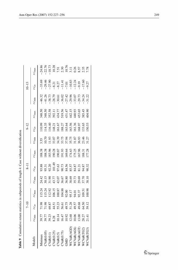
Ann Oper Res (2007) 152:227–256 249

Tabl

e9

Cu

mu

lati

ve

retu

rnst

atis

tics

insu

bp

erio

ds

of

len

gth

4:

Cas

ew

ith

ou

td

iver

sifi

cati

on

7–

10

8–

11

9–

12

10

–1

3

Mo

del

src

min

rcav

rcm

axrc

min

rcav

rcm

axrc

min

rcav

rcm

axrc

min

rcav

rcm

ax

Min

imax

39

.77

71

.98

11

5.2

42

4.4

29

3.8

81

88

.38

3.5

51

10

.99

34

8.5

0−4

6.3

2−3

3.6

9−2

4.8

6

CV

aR(0

.05

)3

9.7

77

1.9

81

15

.24

30

.15

95

.31

18

8.3

81

0.7

01

14

.35

34

8.5

0−4

1.2

6−2

9.4

6−2

2.7

6

CV

aR(0

.1)

39

.23

69

.87

11

2.9

23

1.9

09

2.2

01

83

.96

11

.93

11

6.4

03

52

.58

−38

.73

−27

.90

−18

.73

CV

aR(0

.25

)8

.28

44

.51

10

6.1

54

3.7

71

01

.49

19

0.2

83

3.0

71

48

.21

39

2.1

1−2

8.7

9−8

.21

10

.28

CV

aR(0

.5)

10

.14

55

.23

10

0.8

74

2.0

79

7.6

31

90

.87

34

.39

16

1.6

74

34

.77

−30

.61

−8.2

77

.51

CV

aR(0

.75

)1

6.4

75

6.6

11

04

.88

36

.67

90

.73

19

1.9

33

3.7

51

88

.27

51

9.5

6−3

6.0

2−1

1.4

12

.30

GM

D1

0.9

24

9.7

59

2.0

03

6.8

08

4.5

61

69

.64

37

.94

16

3.6

44

31

.47

−27

.42

−7.0

11

0.7

6

WC

VaR

(AG

D)

12

.68

51

.28

95

.17

38

.69

85

.57

17

4.6

33

5.7

51

63

.56

44

2.1

5−2

9.9

6−1

0.8

33

.11

WC

VaR

(AG

S)

10

.06

49

.57

94

.01

35

.73

84

.87

17

5.2

53

1.8

71

61

.36

44

0.9

3−3

3.0

7−1

2.2

40

.26

WC

VaR

(AG

T)

13

.00

49

.68

92

.37

29

.69

81

.21

16

7.9

63

6.9

31

68

.97

45

3.6

5−2

9.7

3−9

.19

8.5

7

WC

VaR

(TG

2)

28

.27

64

.50

10

9.5

13

7.7

09

4.8

71

88

.31

23

.46

13

3.6

53

85

.45

−34

.24

−17

.60

2.3

5

WC

VaR

(TG

3)

21

.41

59

.12

10

0.9

83

8.1

09

0.3

21

77

.28

31

.27

15

0.5

34

04

.90

−31

.22

−9.2

77

.78

Springer

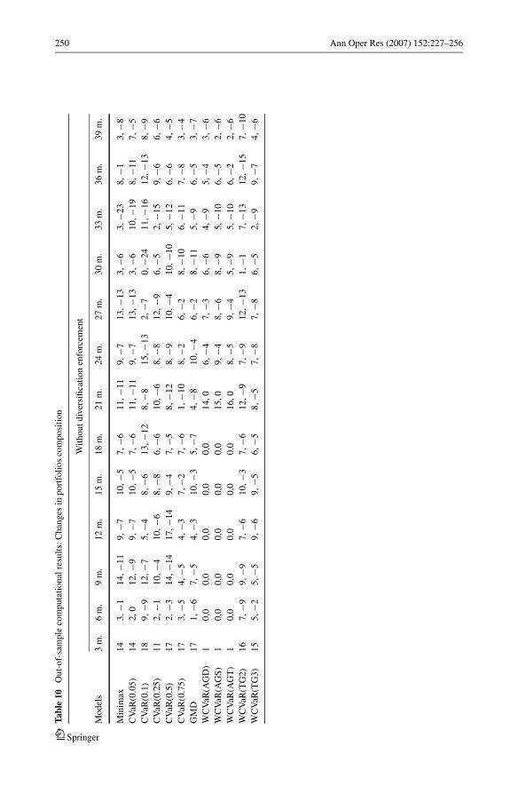
250 Ann Oper Res (2007) 152:227–256

Tabl

e10

Ou

t-o

f-sa

mp

leco

mp

uta

tio

nal

resu

lts:

Ch

ang

esin

po

rtfo

lio

sco

mp

osi

tio

n

Wit

ho

ut

div

ersi

fica

tio

nen

forc

emen

t

Mo

del

s3

m.

6m

.9

m.

12

m.

15

m.

18

m.

21

m.

24

m.

27

m.

30

m.

33

m.

36

m.

39

m.

Min

imax

14

3,−1

14

,−1

19

,−7

10

,−5

7,−6

11

,−1

19

,−7

13

,−1

33

,−6

3,−2

38

,−1

3,−8

CV

aR(0

.05

)1

42

,0

12

,−9

9,−7

10

,−5

7,−6

11

,−1

19

,−7

13

,−1

33

,−6

10

,−1

98

,−1

17

,−5

CV

aR(0

.1)

18

9,−9

12

,−7

5,−4

8,−6

13

,−1

28

,−8

15

,−1

32

,−7

0,−2

41

1,−1

61

2,−1

38

,−9

CV

aR(0

.25

)1

12

,−1

10

,−4

10

,−6

8,−8

6,−6

10

,−6

8,−8

12

,−9

6,−5

2,−1

59

,−6

6,−6

CV

aR(0

.5)

17

2,−3

14

,−1

41

7,−1

49

,−4

7,−5

8,−1

28

,−9

10

,−4

10

,−1

05

,−1

26

,−6

4,−5

CV

aR(0

.75

)1

73

,−5

4,−5

4,−3

7,−2

7,−6

1,−1

08

,−2

6,−2

8,−1

06

,−1

17

,−8

3,−4

GM

D1

71

,−6

7,−5

4,−3

10

,−3

5,−7

4,−8

10

,−4

6,−2

8,−1

15

,−9

6,−5

3,−7

WC

VaR

(AG

D)

10

,00

,00

,00

,00

,01

4,0

6,−4

7,−3

6,−6

4,−9

5,−4

3,−6

WC

VaR

(AG

S)

10

,00

,00

,00

,00

,01

5,0

9,−4

8,−6

8,−9

5,−1

06

,−5

2,−6

WC

VaR

(AG

T)

10

,00

,00

,00

,00

,01

6,0

8,−5

9,−4

5,−9

5,−1

06

,−2

2,−6

WC

VaR

(TG

2)

16

7,−9

9,−9

7,−6

10

,−3

7,−6

12

,−9

7,−9

12

,−1

31

,−1

7,−1

31

2,−1

57

,−1

0

WC

VaR

(TG

3)

15

5,−2

5,−5

9,−6

9,−5

6,−5

8,−5

7,−8

7,−8

6,−5

2,−9

9,−7

4,−6

Springer

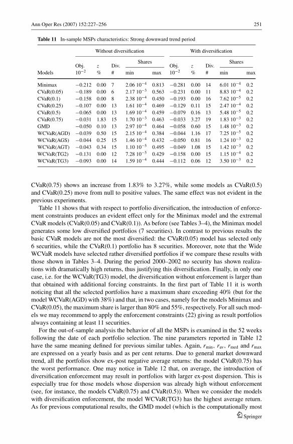
Ann Oper Res (2007) 152:227–256 251

Table 11 In-sample MSPs characteristics: Strong downward trend period

Without diversification With diversification

Shares SharesObj. z Div. Obj. z Div.

Models 10−2 % # min max 10−2 % # min max

Minimax −0.212 0.00 7 2.06 10−4 0.813 −0.281 0.00 14 6.01 10−4 0.2

CVaR(0.05) −0.189 0.00 6 2.17 10−3 0.563 −0.231 0.00 11 8.83 10−4 0.2

CVaR(0.1) −0.158 0.00 8 2.38 10−4 0.450 −0.193 0.00 16 7.62 10−5 0.2

CVaR(0.25) −0.107 0.00 13 1.61 10−4 0.469 −0.129 0.11 15 2.47 10−4 0.2

CVaR(0.5) −0.065 0.00 13 1.69 10−4 0.459 −0.079 0.16 13 5.48 10−5 0.2

CVaR(0.75) −0.031 1.83 15 1.70 10−3 0.463 −0.033 3.27 19 1.83 10−3 0.2

GMD −0.050 0.10 13 2.97 10−4 0.464 −0.058 0.60 15 1.48 10−3 0.2

WCVaR(AGD) −0.039 0.50 15 2.15 10−4 0.384 −0.044 1.16 17 7.25 10−5 0.2

WCVaR(AGS) −0.044 0.25 15 1.46 10−4 0.432 −0.050 0.81 16 1.24 10−3 0.2

WCVaR(AGT) −0.043 0.34 15 1.10 10−5 0.495 −0.049 1.08 15 1.42 10−3 0.2

WCVaR(TG2) −0.131 0.00 12 7.28 10−5 0.429 −0.158 0.00 15 1.15 10−4 0.2

WCVaR(TG3) −0.093 0.00 14 1.59 10−4 0.444 −0.112 0.06 12 3.50 10−3 0.2

CVaR(0.75) shows an increase from 1.83% to 3.27%, while some models as CVaR(0.5)

and CVaR(0.25) move from null to positive values. The same effect was not evident in the

previous experiments.

Table 11 shows that with respect to portfolio diversification, the introduction of enforce-

ment constraints produces an evident effect only for the Minimax model and the extremal

CVaR models (CVaR(0.05) and CVaR(0.1)). As before (see Tables 3–4), the Minimax model

generates some low diversified portfolios (7 securities). In contrast to previous results the

basic CVaR models are not the most diversified: the CVaR(0.05) model has selected only

6 securities, while the CVaR(0.1) portfolio has 8 securities. Moreover, note that the Wide

WCVaR models have selected rather diversified portfolios if we compare these results with

those shown in Tables 3–4. During the period 2000–2002 no security has shown realiza-

tions with dramatically high returns, thus justifying this diversification. Finally, in only one

case, i.e. for the WCVaR(TG3) model, the diversification without enforcement is larger than

that obtained with additional forcing constraints. In the first part of Table 11 it is worth

noticing that all the selected portfolios have a maximum share exceeding 40% (but for the

model WCVaR(AGD) with 38%) and that, in two cases, namely for the models Minimax and

CVaR(0.05), the maximum share is larger than 80% and 55%, respectively. For all such mod-

els we may recommend to apply the enforcement constraints (22) giving as result portfolios

always containing at least 11 securities.

For the out-of-sample analysis the behavior of all the MSPs is examined in the 52 weeks

following the date of each portfolio selection. The nine parameters reported in Table 12

have the same meaning defined for previous similar tables. Again, rmin, rav, rmed and rmax

are expressed on a yearly basis and as per cent returns. Due to general market downward

trend, all the portfolios show ex-post negative average returns: the model CVaR(0.75) has

the worst performance. One may notice in Table 12 that, on average, the introduction of

diversification enforcement may result in portfolios with larger ex-post dispersion. This is

especially true for those models whose dispersion was already high without enforcement

(see, for instance, the models CVaR(0.75) and CVaR(0.5)). When we consider the models

with diversification enforcement, the model WCVaR(TG3) has the highest average return.

As for previous computational results, the GMD model (which is the computationally most

Springer

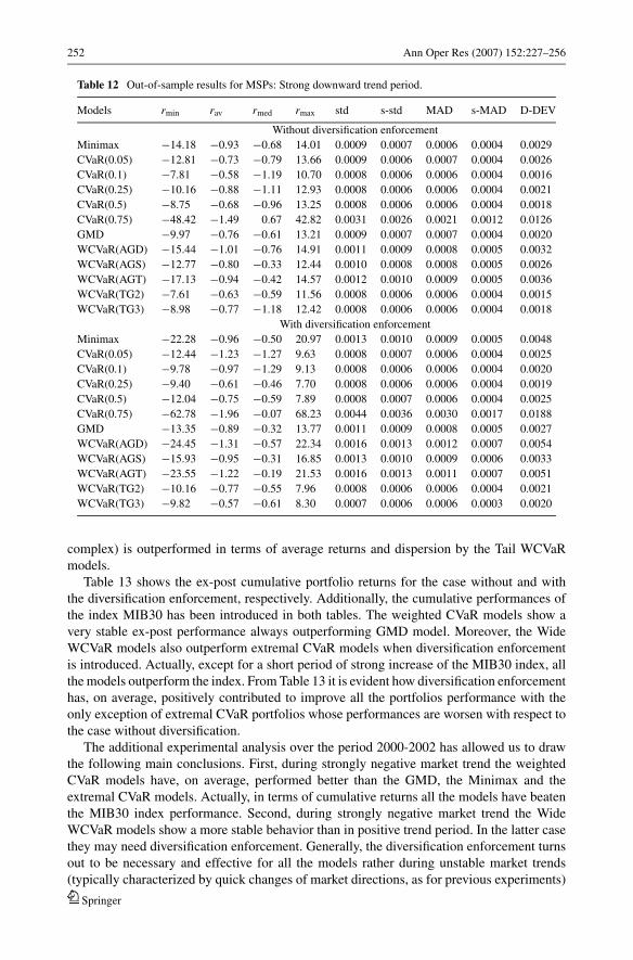
252 Ann Oper Res (2007) 152:227–256

Table 12 Out-of-sample results for MSPs: Strong downward trend period.

Models rmin rav rmed rmax std s-std MAD s-MAD D-DEV

Without diversification enforcement

Minimax −14.18 −0.93 −0.68 14.01 0.0009 0.0007 0.0006 0.0004 0.0029

CVaR(0.05) −12.81 −0.73 −0.79 13.66 0.0009 0.0006 0.0007 0.0004 0.0026

CVaR(0.1) −7.81 −0.58 −1.19 10.70 0.0008 0.0006 0.0006 0.0004 0.0016

CVaR(0.25) −10.16 −0.88 −1.11 12.93 0.0008 0.0006 0.0006 0.0004 0.0021

CVaR(0.5) −8.75 −0.68 −0.96 13.25 0.0008 0.0006 0.0006 0.0004 0.0018

CVaR(0.75) −48.42 −1.49 0.67 42.82 0.0031 0.0026 0.0021 0.0012 0.0126

GMD −9.97 −0.76 −0.61 13.21 0.0009 0.0007 0.0007 0.0004 0.0020

WCVaR(AGD) −15.44 −1.01 −0.76 14.91 0.0011 0.0009 0.0008 0.0005 0.0032

WCVaR(AGS) −12.77 −0.80 −0.33 12.44 0.0010 0.0008 0.0008 0.0005 0.0026

WCVaR(AGT) −17.13 −0.94 −0.42 14.57 0.0012 0.0010 0.0009 0.0005 0.0036

WCVaR(TG2) −7.61 −0.63 −0.59 11.56 0.0008 0.0006 0.0006 0.0004 0.0015

WCVaR(TG3) −8.98 −0.77 −1.18 12.42 0.0008 0.0006 0.0006 0.0004 0.0018

With diversification enforcement

Minimax −22.28 −0.96 −0.50 20.97 0.0013 0.0010 0.0009 0.0005 0.0048

CVaR(0.05) −12.44 −1.23 −1.27 9.63 0.0008 0.0007 0.0006 0.0004 0.0025

CVaR(0.1) −9.78 −0.97 −1.29 9.13 0.0008 0.0006 0.0006 0.0004 0.0020

CVaR(0.25) −9.40 −0.61 −0.46 7.70 0.0008 0.0006 0.0006 0.0004 0.0019

CVaR(0.5) −12.04 −0.75 −0.59 7.89 0.0008 0.0007 0.0006 0.0004 0.0025

CVaR(0.75) −62.78 −1.96 −0.07 68.23 0.0044 0.0036 0.0030 0.0017 0.0188

GMD −13.35 −0.89 −0.32 13.77 0.0011 0.0009 0.0008 0.0005 0.0027

WCVaR(AGD) −24.45 −1.31 −0.57 22.34 0.0016 0.0013 0.0012 0.0007 0.0054

WCVaR(AGS) −15.93 −0.95 −0.31 16.85 0.0013 0.0010 0.0009 0.0006 0.0033

WCVaR(AGT) −23.55 −1.22 −0.19 21.53 0.0016 0.0013 0.0011 0.0007 0.0051

WCVaR(TG2) −10.16 −0.77 −0.55 7.96 0.0008 0.0006 0.0006 0.0004 0.0021

WCVaR(TG3) −9.82 −0.57 −0.61 8.30 0.0007 0.0006 0.0006 0.0003 0.0020

complex) is outperformed in terms of average returns and dispersion by the Tail WCVaR

models.

Table 13 shows the ex-post cumulative portfolio returns for the case without and with

the diversification enforcement, respectively. Additionally, the cumulative performances of

the index MIB30 has been introduced in both tables. The weighted CVaR models show a

very stable ex-post performance always outperforming GMD model. Moreover, the Wide

WCVaR models also outperform extremal CVaR models when diversification enforcement

is introduced. Actually, except for a short period of strong increase of the MIB30 index, all

the models outperform the index. From Table 13 it is evident how diversification enforcement

has, on average, positively contributed to improve all the portfolios performance with the

only exception of extremal CVaR portfolios whose performances are worsen with respect to

the case without diversification.

The additional experimental analysis over the period 2000-2002 has allowed us to draw

the following main conclusions. First, during strongly negative market trend the weighted

CVaR models have, on average, performed better than the GMD, the Minimax and the

extremal CVaR models. Actually, in terms of cumulative returns all the models have beaten

the MIB30 index performance. Second, during strongly negative market trend the Wide

WCVaR models show a more stable behavior than in positive trend period. In the latter case

they may need diversification enforcement. Generally, the diversification enforcement turns

out to be necessary and effective for all the models rather during unstable market trends

(typically characterized by quick changes of market directions, as for previous experiments)

Springer

Ann Oper Res (2007) 152:227–256 253

than during strong downward periods where for some models, as for the extremal CVaR

models, diversification enforcement has made performances even worse.

4 Concluding remarks

In this paper we have studied LP solvable portfolio optimization models based on exten-

sions of the Conditional Value at Risk (CVaR) measure. The models use multiple CVaR

measures thus allowing for more detailed risk aversion modeling. All the studied models

are SSD consistent and may be considered some approximations to the Gini’s mean dif-

ference with the advantage of being computationally much simpler than the GMD model

itself. Our analysis has been focused on the weighted CVaR measures defined as sim-

ple combinations of a very few CVaR measures. We have introduced two specific types

of weight-settings which relate the WCVaR measure to the Gini’s mean difference (the

Wide WCVaR) and its tail version (the Tail WCVaR). This allows us to use a few tolerance

levels as only parameters specifying the entire WCVaR measures while the correspond-

ing weights are automatically predefined by the requirements of the corresponding Gini’s

measures.

Our experimental analysis of the models performance on the real-life data from the Mi-

lan Stock Exchange has confirmed their attractiveness. The WCVaR models have usually

performed better than the GMD, the Minimax or the extremal CVaR models. These promis-

ing results show a need for further comprehensive experimental studies analyzing practical

performances of the WCVaR models within specific areas of financial applications. It is im-

portant to notice that although the quantile risk measures (VaR and CVaR) were introduced in

banking as extreme risk measures for small tolerance levels (like β = 0.05), for the portfolio

optimization good results have been provided by rather larger tolerance levels. Additional

experimental analysis over the period with strongly negative market trend has confirmed

good achievements of the WCVaR models. In terms of cumulative returns all the models

have outperformed the MIB30 index.

While the Tail WCVaR models have always generated well diversified portfolios,

the Wide WCVaR models require some diversification enforcement to avoid too small

portfolios. Our experiments have also confirmed effectiveness of our CVaR based tech-

nique for a direct diversification enforcement. Although, the diversification enforce-

ment turns out to be necessary and effective rather during unstable market trends (typi-

cally characterized by quick changes of market directions) than during strong downward

periods.

Appendix

The spectral risk measures have been shown to be coherent in the sense of Artzner et al.

(1999). These coherence axioms are based on the standard ‘monotonicity’ (X ≥ Y a.s. ⇒ρ(X ) ≤ ρ(Y )). Since the measures represent the dual theory of choice (Yaari, 1987), they

should also satisfy stronger monotonicity related to the SSD dominance. Indeed, the following

SSD consistency results can be shown.

Theorem 3. If a nonnegative real function φ on the interval [0, 1] is weakly decreasing (i.e.,α1 < α2 implies φ(α1) ≥ φ(α2)), then the spectral measure Mφ(x) = ∫ 1

0φ(α)F (−1)

x (α)dα is

Springer

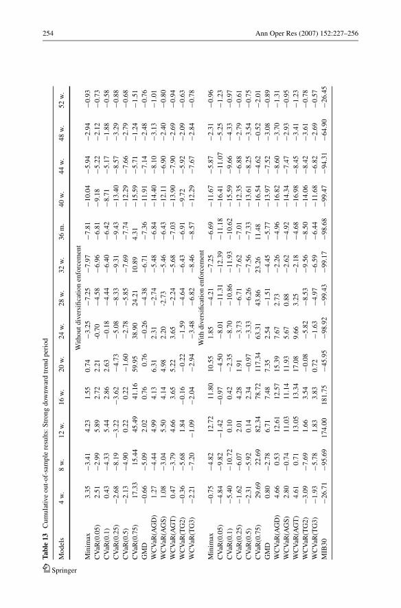
254 Ann Oper Res (2007) 152:227–256

Tabl

e13

Cu

mu

lati

ve

ou

t-o

f-sa

mp

lere

sult

s:S

tro

ng

dow

nw

ard

tren

dp

erio

d

Mo

del

s4

w.

8w

.1

2w

.1

6w

.2

0w

.2

4w

.2

8w

.3

2w

.3

6m

.4

0w

.4

4w

.4

8w

.5

2w

.

Wit

ho

ut

div

ersi

fica

tio

nen

forc

emen

t

Min

imax

3.3

5−3

.41

4.2

31

.55

0.7

4−3

.25

−7.2

5−7

.97

−7.8

1−1

0.0

4−5

.94

−2.9

4−0

.93

CV

aR(0

.05

)2

.51

−2.9

95

.89

2.7

22

.21

-0.7

0−4

.58

−6.9

6−6

.81

−9.1

8−5

.22

−2.1

2−0

.73

CV

aR(0

.1)

0.4

3−4

.33

5.4

42

.86

2.6

3−0

.18

−4.4

4−6

.40

−6.4

2−8

.71

−5.1

7−1

.88

−0.5

8

CV

aR(0

.25

)−2

.68

−8.1

9−3

.22

−3.6

2−4

.73

−5.0

8−8

.33

−9.3

1−9

.43

−13

.40

−8.5

7−3

.29

−0.8

8

CV

aR(0

.5)

−2.1

3−4

.90

0.2

20

.22

−1.6

0−2

.78

−5.8

5−7

.69

−7.7

4−1

2.2

9− 7

.66

−2.7

9−0

.68

CV

aR(0

.75

)1

7.3

31

5.4

44

5.4

94

1.1

65

9.9

53

8.9

02

4.2

11

0.8

94

.31

−15

.59

−5.7

1−1

.24

−1.5

1

GM

D−0

.66

−5.0

92

.02

0.7

60

.76

−0.2

6−4

.38

−6.7

1−7

.36

−11

.91

−7.1

4−2

.48

−0.7

6

WC

VaR

(AG

D)

1.2

7−4

.44

4.9

94

.13

6.3

12

.31

−2.7

4−5

.48

−6.8

4−1

4.4

0−8

.10

−3.1

3−1

.01

WC

VaR

(AG

S)

1.0

8−3

.04

5.5

04

.14

4.9

82

.20

-2.7

3−5

.46

−6.4

3−1

2.1

1−6

.90

−2.4

0−0

.80

WC

VaR

(AG

T)

0.4

7−3

.79

4.6

63

.65

5.2

23

.65

−2.2

4−5

.68

−7.0

3−1

3.9

0−7

.90

−2.6

9−0

.94

WC

VaR

(TG

2)

−0.3

6−5

.68

1.8

4−0

.16

−0.2

2−1

.59

−4.6

4−6

.43

−6.9

1−9

.72

−5.9

2−2

.09

−0.6

3

WC

VaR

(TG

3)

−2.2

1−7

.20

−1.0

9−2

.04

−2.9

4−3

.48

−6.8

2−8

.46

−8.5

7−1

2.2

9−7

.67

−2.8

4−0

.78

Wit

hd

iver

sifi

cati

on

enfo

rcem

ent

Min

imax

−0.7

5−4

.82

12

.72

11

.80

10

.55

1.8

5−4

.21

−7.2

5−6

.69

−11

.67

−5.8

7−2

.31

−0.9

6

CV

aR(0

.05

)−4

.84

−9.8

2−1

.42

−0.9

7−4

.50

−8.0

1−1

1.3

1−1

2.3

9−1

1.1

8−1

6.4

1−1

1.0

7−5

.25

−1.2

3

CV

aR(0

.1)

−5.4

0−1

0.7

20

.10

0.4

2−2

.35

−8.7

0−1

0.8

6−1

1.9

3−1

0.6

2−1

5.5

9−9

.66

−4.3

3−0

.97

CV

aR(0

.25

)−1

.62

−6.0

72

.01

4.2

81

.91

−3.7

3−6

.71

−7.6

2−7

.01

−12

.35

−6.8

8−2

.79

−0.6

1

CV

aR(0

.5)

−2.3

1−5

.92

0.1

42

.34

−0.9

7−3

.33

−6.2

6−7

.56

−7.3

3−1

3.6

1−8

.25

−3.5

4−0

.75

CV

aR(0

.75

)2

9.6

92

2.6

98

2.3

47

8.7

21

17

.34

63

.31

43

.86

23

.26

11

.48

−16

.54

−4.6

2−0

.52

−2.0

1

GM

D0

.80

−2.7

86

.71

7.4

87

.35

2.5

4−1

.51

−4.4

5−5

.77

−13

.97

−7.5

2−3

.08

−0.8

9

WC

VaR

(AG

D)

4.6

60

.53

12

.61

12

.57

15

.39

7.6

72

.73

−2.2

6−4

.96

−16

.82

−8.6

0−3

.70

−1.3

1

WC

VaR

(AG

S)

2.8

0−0

.74

11

.03

11

.14

11

.93

5.6

70

.88

−2.6

2−4

.92

−14

.34

−7.4

7−2

.93

− 0.9

5

WC

VaR

(AG

T)

4.6

10

.71

13

.05

13

.34

17

.08

9.6

63

.25

−2.1

8−4

.68

−16

.98

−8.4

5−3

.41

−1.2

3

WC

VaR

(TG

2)

−3.0

9−7

.69

1.6

63

.54

−0.0

8−5

.82

−8.5

3−9

.56

−8.5

0−1

4.0

6−8

.42

−3.6

1−0

.78

WC

VaR

(TG

3)

−1.9

3−5

.78

1.8

33

.83

0.7

2−1

.63

−4.9

7−6

.59

−6.4

4−1

1.6

8−6

.82

−2.6

9−0

.57

MIB

30

−26

.71

−95

.69

17

4.0

01

81

.75

−45

.95

−98

.92

−99

.43

−99

.17

−98

.68

−99

.47

−94

.31

−64

.90

−26

.45

Springer

Ann Oper Res (2007) 152:227–256 255

SSD consistent, i.e.,

Rx′ �SSD Rx′′ ⇒ Mφ(x′) ≥ Mφ(x′′).

Proof: Note that Mφ(x′) − Mφ(x′′) = ∫ 1

0φ(α)(F (−1)

x′ (α) − F (−1)x′′ (α))dα and integrating by

parts one gets

Mφ(x′) − Mφ(x′′) = φ(1)(F (−2)

x′ (1) − F (−2)x′′ (1)

) −∫ 1

0

(F (−2)

x′ (α) − F (−2)x′′ (α)

)dφ(α) (22)

If Rx′ �SSD Rx′′ , then F (−2)x′ (α) ≥ F (−2)

x′′ (α) for all α ∈ [0, 1] and, in particular, F (−2)x′ (1) −

F (−2)x′′ (1) = μ(x′) − μ(x′′) ≥ 0. Hence, due to assumed properties of function φ, one gets

Mφ(x′) − Mφ(x′′) ≥ 0. �

Theorem 4. If a nonnegative real function φ on the interval [0, 1] is strictly decreasing (i.e.,α1 < α2 implies φ(α1) > φ(α2)), then the spectral measure Mφ(x) = ∫ 1

0φ(α)F (−1)

x (α)dα isstrictly SSD consistent, i.e.,

Rx′ SSD Rx′′ ⇒ Mφ(x′) > Mφ(x′′).

Proof: If Rx′ SSD Rx′′ , then F (−2)x′ (α) ≥ F (−2)

x′′ (α) for all α ∈ [0, 1] with at least one strict

inequality for some α0 ∈ (0, 1]. Moreover, F (−2)x are continuous functions (Ogryczak and

Ruszczynski, 2002a). Therefore, there exist ε > 0 such that F (−2)x′ (α) > F (−2)

x′′ (α) for all α ∈(α0 − ε, α0]. Hence, due to assumed properties of function φ, using (22) one gets Mφ(x′) −Mφ(x′′) > 0, which completes the proof. �

Acknowledgements The authors wish to thank Gianfranco Guastaroba for valuable help in carrying outcomputational results. Research conducted by W. Ogryczak was supported by the grant 3T11C 005 27 fromThe State Committee for Scientific Research (Poland).

References

Acerbi, C. (2002).“Spectral Measures of Risk: A Coherent Representation of Subjective Risk Aversion.”Journal of Banking & Finance, 26, 1505–1518.

Acerbi, C. and P. Simonetti. (2002). “Portfolio Optimization with Spectral Measures of Risk.” Working Paper(http://gloriamundi.org).

Andersson, F., H. Mausser, D. Rosen, and S. Uryasev. (2001). “Credit Risk Optimization with ConditionalValue-at-Risk Criterion.” Mathematical Programming, 89, 273–291.

Artzner, P., F. Delbaen, J.-M. Eber, and D. Heath. (1999). “Coherent Measures of Risk.” Mathematical Finance,9, 203–228.

Chiodi, L., R. Mansini, and M.G. Speranza. (2003). “Semi-Absolute Deviation Rule for Mutual Funds PortfolioSelection.” Annals of Operations Research, 124, 245–265.

Embrechts, P., C. Kluppelberg, and T. Mikosch. (1997). Modelling Extremal Events for Insurance and Finance.New York: Springer-Verlag.

Haimes, Y.Y. (1993). “Risk of Extreme Events and the Fallacy of the Expected Value.” Control and Cybernetics,22, 7–31.

Jorion, P. (2001). Value-at-Risk: The New Benchmark for Managing Financial Risk. NY: McGraw-Hill.Kellerer, H., R. Mansini, and M.G. Speranza. (2000). “Selecting Portfolios with Fixed Costs and Minimum

Transaction Lots.” Annals of Operations Research, 99, 287–304.Konno, H., and H. Yamazaki. (1991). “Mean-Absolute Deviation Portfolio Optimization Model and Its Ap-

plication to Tokyo Stock Market.” Management Science, 37, 519–531.Konno, H., and A. Wijayanayake. (2001). “Portfolio Optimization Problem under Concave Transaction Costs

and Minimal Transaction Unit Constraints.” Mathematical Programming, 89, 233–250.Levy, H., and Y. Kroll. (1978). “Ordering Uncertain Options with Borrowing and Lending.” Journal of Finance,

33, 553–573.

Springer

256 Ann Oper Res (2007) 152:227–256

Mansini, R., W. Ogryczak, and M.G. Speranza. (2003a). “On LP Solvable Models for Portfolio Selection.”Informatica, 14, 37–62.

Mansini, R., W. Ogryczak, and M.G. Speranza. (2003b). “LP Solvable Models for Portfolio Optimization: AClassification and Computational Comparison.” IMA J. of Management Mathematics, 14, 187–220.

Mansini, R., W. Ogryczak, and M.G. Speranza. (2003c). “Conditional Value at Risk and Related LinearProgramming Models for Portfolio Optimization.” Tech. Report 03–02, Warsaw Univ. of Technology.

Mansini, R. and M.G. Speranza. (1999). “Heuristic Algorithms for the Portfolio Selection Problem withMinimum Transaction Lots.” European J. of Operational Research, 114, 219–233.

Mansini, R. and M.G. Speranza. (2005). “An Exact Approach for the Portfolio Selection Problem with Trans-action Costs and Rounds.” IIE Transactions, 37, 919–929.

Markowitz, H.M. (1952). “Portfolio Selection.” Journal of Finance, 7, 77–91.Ogryczak, W. (1999). “Stochastic Dominance Relation and Linear Risk Measures.” In A.M.J. Skulimowski

(ed.), Financial Modelling—Proceedings of the 23rd Meeting of the EURO Working Group on FinancialModelling. Cracow: Progress & Business Publ., 191–212.

Ogryczak, W. (2000). “Multiple Criteria Linear Programming Model for Portfolio Selection.” Annals ofOperations Research, 97, 143–162.

Ogryczak, W. (2002). “Multiple Criteria Optimization and Decisions under Risk.” Control and Cybernetics,31, 975–1003.

Ogryczak, W. and A. Ruszczynski. (1999). “From Stochastic Dominance to Mean-Risk Models: Semidevia-tions as Risk Measures.” European J. of Operational Research, 116, 33–50.

Ogryczak, W. and A. Ruszczynski. (2001). “On Stochastic Dominance and Mean-Semideviation Models.”Mathematical Programming, 89, 217–232.

Ogryczak, W. and A. Ruszczynski. (2002a). “Dual Stochastic Dominance and Related Mean-Risk Models.”SIAM J. on Optimization, 13, 60–78.

Ogryczak, W. and A. Ruszczynski. (2002b). “Dual Stochastic Dominance and Quantile Risk Measures.”International Transactions in Operational Research, 9, 661–680.

Ogryczak, W. and A. Tamir. (2003). “Minimizing the Sum of the k-Largest Functions in Linear Time.”Information Processing Letters, 85, 117–122.

Pflug, G.Ch. (2000). “Some Remarks on the Value-at-Risk and the Conditional Value-at-Risk.” In S.Uryasev(ed.), Probabilistic Constrained Optimization: Methodology and Applications, Dordrecht: Kluwer A.P.

Rockafellar, R.T. and S. Uryasev. (2000). “Optimization of Conditional Value-at-Risk.” Journal of Risk, 2,21–41.

Rockafellar, R.T. and S. Uryasev. (2002). “Conditional Value-at-Risk for General Distributions.” Journal ofBanking & Finance, 26, 1443–1471.

Rockafellar, R.T., S. Uryasev, and M. Zabarankin. (2002). “Deviation Measures in Generalized Linear Re-gression.” Research Report 2002-9, Univ. of Florida, ISE.

Rothschild, M. and J.E. Stiglitz. (1969). “Increasing Risk: I. A Definition.” Journal of Economic Theory, 2,225–243.

Shalit, H. and S. Yitzhaki. (1994). “Marginal Conditional Stochastic Dominance.” Management Science, 40,670–684.

Sharpe, W.F. (1971a). “A Linear Programming Approximation for the General Portfolio Analysis Problem.”Journal of Financial and Quantitative Analysis, 6, 1263–1275.

Sharpe, W.F. (1971b). “Mean-Absolute Deviation Characteristic Lines for Securities and Portfolios.” Man-agement Science, 8, B1–B13.

Shorrocks, A.F. (1983). “Ranking Income Distributions.” Economica, 50, 3–17.Simaan, Y. (1997). “Estimation Risk in Portfolio Selection: The Mean Variance Model and the Mean-Absolute

Deviation Model.” Management Science, 43, 1437–1446.Speranza, M.G. (1993). “Linear Programming Models for Portfolio Optimization.” Finance, 14, 107–123.Topaloglou, N., H. Vladimirou, and S.A. Zenios. (2002). “CVaR Models with Selective Hedging for Interna-

tional Asset Allocation.” Journal of Banking & Finance, 26, 1535–1561.Whitmore, G.A., and M.C. Findlay (eds.). (1978). Stochastic Dominance: An Approach to Decision–Making

Under Risk. Lexington MA: D.C.Heath.Yaari, M.E. (1987). “The Dual Theory of Choice under Risk.” Econometrica, 55, 95–115.Yitzhaki, S. (1982). “Stochastic Dominance, Mean Variance, and Gini’s Mean Difference.” American Eco-

nomic Revue, 72, 178–185.Young, M.R. (1998). “A Minimax Portfolio Selection Rule with Linear Programming Solution.” Management

Science, 44, 673–683.

Springer