Conditional Gaussian Distributions

Bayesian Scientific Computing, Spring 2013 (N. Zabaras)

Conditional Gaussian Distributions

Prof. Nicholas Zabaras

Materials Process Design and Control Laboratory

Sibley School of Mechanical and Aerospace Engineering

101 Frank H. T. Rhodes Hall

Cornell University

Ithaca, NY 14853-3801

Email: [email protected]

URL: http://mpdc.mae.cornell.edu/

January 23, 2014

1

mailto:[email protected]

http://mpdc.mae.cornell.edu/



The Precision Matrix

Completing the Square

The Conditional Distribution, Conditional Mean and Variance Formulas,

The Marginal Distribution, Summary of Marginals/Conditionals

2D Distributions Example

Interpolating Noise-Free Data

Data Imputation

Contents

2

Chris Bishop, Pattern Recognition and Machine Learning, Chapter 2

Kevin Murphy, Machine Learning: A probabilistic Perspective, Chapter 4

http://research.microsoft.com/en-us/um/people/cmbishop/prml/

http://www.cs.ubc.ca/~murphyk/MLbook/


If two sets of variables are jointly Gaussian, then the

conditional distribution of one set conditioned on the other is

again Gaussian.

Suppose x is a D-dimensional vector with Gaussian

distribution N(x|μ,Σ) and that we partition x into two disjoint

subsets xa (M components) and xb (D-M components).


3

a

b

xx =

x


This partition also implies similar partitions for the mean and

covariance.

ΣT = Σ implies that Σaa and Σbb are symmetric and


4

,a aa ab

b ba bb

=

T

ba ab


We define the precision matrix L as -1.

Its partition is given as above

where from ΣT = Σ we conclude that Laa and Lbb are

symmetric (the inverse of a symmetric matrix is symmetric)

and

Note that the above partition does NOT imply that Laa is the

inverse of aa , etc.

The Precision Matrix

5

aa ab

ba bb

L LL

L L

T

ba abL L


We are given a quadratic form defining the exponent terms in

a Gaussian distribution, and we determine the corresponding

mean and covariance.

The constant term denotes terms independent of x.

If we are given only the right hand side, we can immediately

identify from the 1st quadratic in x term the inverse of the

covariance matrix and subsequently from the 2nd linear in x

term the mean of the distribution.

This approach is used often in analytical calculations.

Completing the Square

6

1 1 11 1( ) ( )

2 2

T T T constant- - -- - - - x x x x x


We are now interested to compute p(xa|xb).

An easy way to do that is to look at the joint distribution

p(xa,xb) considering xb constant.

Using the partition of the precision matrix, we can write:

The Conditional Distribution

7

11 1 1( ) ( ) ( ) ( ) ( ) ( )

2 2 2

1 1( ) ( ) ( ) ( )

2 2

T T T

a a aa a a a a ab b b

T T

b b ba a a b b bb b b

-- - - - - - - - -

- - - - - -

x x x x x x

x x x x

L L

L L


We fix xb and consider the distribution above in terms of xa. It

is quadratic so we have a Gaussian. We need to complete the

square in xa.

In conclusion:


8

11 1 1( ) ( ) ( ) ( ) ( ) ( )

2 2 2

1 1( ) ( ) ( ) ( )

2 2

T T T


T T


-- - - - - - - - -

- - - - - -

x x x x x x

x x x x

L L

L L

1

| ( )a b a aa ab b b

- - -x L L

1

|

1:

2

T

a aa a a b aaQuadratic term -- x xL L

1

| |: ( ) ( )T

a aa a ab b b a b a b aa a ab b bLinear term -- - - - x x x L L L L

1

|| | , -a b a a b aap Nx x x L 1


- - -x L L


We can also write (with more complicated expressions) the

previous results in terms of the partitioned covariance

matrix.

We can show that the following result holds:

where

This is called the partitioned inverse formula. M is the

Schur complement of our matrix with respect to D.

The Partitioned Inverse Formula

9

1 1 1

1 1,

-- - -

- -

-1

-1 -1 -1 -1

A B M M BD

C D -D CM D D CM BD

-1M A - BD C


Step 1.

Step 2.

Step 3. Combining the steps above (with ):

Partitioned Inverse Formula: Proof

10

1 1 1

1 1

-- - -

- -

-1

-1 -1 -1 -1

A B M M BD

C D -D CM D D CM BD

-1M A - BD C

1 1- -- -

0A BI BD A BD C

C D0 I C D

1 1

1

- -

-

- -

-

00 0

0

IA BD C A BD C

D C IC D D

11 11 1 1 1

1 1 1

- - -

- -

0 00 0

0 0

-- -- - - -

- - -

A B I I A BI BD A BD C I BD M

C D D C I D C I C D0 I D 0 I D

1 1 1

1 1

-

-

0 0

0

- - -

- -

A B I M I BD

C D D C I D 0 I


We can also use the Schur complement with respect to A.

This leads to:

We easily test with direct multiplication that the following

result holds:

where

Partitioned Inverse Formula

11

1 1

1 1,

-- -

- -

-1 -1 -1 -1 -1

-1

A B A A BM CA A BM

C D -M CA M

-1M D - CA B


From the two expressions of the inverse formula, we can

derive useful identities

From equating the upper left blocks we obtain:

Similarly equating the top right blocks we obtain:

Finally one can show:

Matrix Inversion Lemma – Sherman Morrison Woodbury Formula

12

1 11

1 1

1 1

1 11

,

-

-

- --

- -

- -

- --

-1 -1 -1

-1 -1 -1 -1 -1 -1

-1 -1 -1 -1 -1 -1

-1 -1

A - BD C A - BD C BDA B

C D -D C A - BD C D D C A - BD C BD

A A B D - CA B CA A B D - CA B

- D - CA B CA D - CA B

1 1- -

-1 -1 -1 -1 -1A - BD C A A B D - CA B CA

1 1- -

-1 -1 -1 -1A - BD C BD A B D - CA B

-1 -1 -1A - BD C D - CA B D A


Woodbury Matrix Inversion Formula

13

In addition to completing the square and the matrix

inversion formula for a partitioned matrix discussed earlier,

the Woodbury matrix inversion formula is quite useful for

manipulating Gaussians:

Consider the following application. Let A= be an NxN

diagonal matrix and let B=CT=X of size NxD where N>>D,

and let D−1 =- IDxD. Then we have

The LHS takes O(N3) time to compute, the RHS takes time

O(D3) to compute.

1 1

1 1 1 1T T T

N N D D

- -

- - - -

-

XX X I X X X

1 1- -

-1 -1 -1 -1 -1A - BD C A A B D - CA B CA


Rank One Update of an Inverse

14

Another useful application arises in computing the rank 1

update of an inverse matrix. Select B=u (a column vector)

and C=vT (a row vector), and let D=-1 (scalar). Then using

We obtain

This is important when we incrementally add (or subtract)

one data point at a time to the design matrix and we want

to update the sufficient statistics.

1 1

1 11 1 1 1 1

11

1

TT T T

T

- -- -

- - - - -

- - -

A uv AA uv A A u v A u v A A

v A u

1 1- -

-1 -1 -1 -1 -1A - BD C A A B D - CA B CA


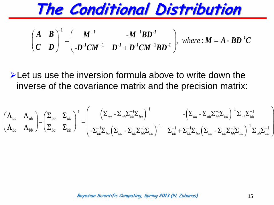
Let us use the inversion formula above to write down the

inverse of the covariance matrix and the precision matrix:


15

1 1 1

1 1, :

-where

- - -

- -

-1

-1

-1 -1 -1 -1

A B M M BDM A - BD C

C D -D CM D D CM BD

1 11 1 11

1 11 1 1 1 1 1

aa ab bb ba aa ab bb ba ab bbaa ab aa ab

ba bb ba bbbb ba aa ab bb ba bb bb ba aa ab bb ba ab bb

-- -

- - --

- -- - - - - -

- -

- - -

L L

L L


We can reverse the previous results as well and write the

partitioned covariance matrix in terms of the inverse of the

partitioned precision matrix:


16

1 1 1

1 1, :

-where

- - -

- -

-1

-1

-1 -1 -1 -1

A B M M BDM A - BD C

C D -D CM D D CM BD

1 11 1 11

1 11 1 1 1 1 1

- -- - --

- -- - - - - -



-- -

- - -

L L L L L L L L L L L L

L L L L L L L L L L L L L L L L L


From the earlier expressions of the conditional mean and

variance, we can write:

Note that the conditional mean is linear in xb and the

conditional variance is independent of xb.


17

1 1

| ( ) ( )a b a aa ab b b a ab bb b b

- - - - -x x L L

1 1

|a b aa aa ab bb ba

- - - L

1 11 1 11

1 11 1 1 1 1 1



-- -

- - --

- -- - - - - -

- -

- - -

L L

L L

| || | ,a b a a b a bp Nx x x


We are now interested to compute p(xa). An easy way to do

this is to look at the joint distribution p(xa,xb) integrating xb out.

Using the partition of the precision matrix, we can write:

The Marginal Distribution

18

11 1 1( ) ( ) ( ) ( ) ( ) ( )

2 2 2

1 1( ) ( ) ( ) ( )

2 2

1( )

2

T T T


T T


T T

b bb b b bb b ba a a bnon dependent terms

-- - - - - - - - -

- - - - - -

- -

m

x x x x x x

x x x x

x x + x - x x

L L

L L

L L L


To integrate xb out, we complete the square in xb.

The first term gives a normalization factor when integrating in

xb.


19

1

( )2

T T

b bb b b bb b ba a a bnon dependent terms- -

m

x x + x - x x L L L

1 1 11 1 1( ) ( )

2 2 2

T T T T

b bb b b b bb bb b bb bb

- - -- - - - x x + x m x m x m m mL L L L L


We are left with the following terms that depend on xa:


20

1

1

1 1

1( ) ( ) ( )

2

1( ) ( )

2

1 1( ) ( )

2 2

1

2

T T

a a aa a a a a ab b

T

bb b ba a a bb bb b ba a a

TT T

a aa a a aa a ab b bb b ba a a bb bb b ba a a

T T

a aa ab bb ba a a aa a ab b ab bb bb b b

-

-

- -

- - - -

- -

- - -

-

x x x

- x - x

x x x x - x

x - x x +

L L

L L L L L

L L L L - L L L L

L L L L L L - L L L L

1 1

...

1...

2

a a

T T

a aa ab bb ba a a aa ab bb ba a

- -

- x - x x

L L L L L - L L L


By completing the square in xa, we can find the covariance

and mean of the marginal:


21

1 11...

2

T T

a aa ab bb ba a a aa ab bb ba a

- -- x - x x L L L L L - L L L

a a x

1

1 11:

2

T

a aa ab bb ba a a aa ab bb ba aaQuadratic term-

- -- x - x -L L L L L L L L

1 1 1: T

a aa ab bb ba a a a aa ab bb ba aLinear term - - - x x L - L L L L - L L L


Conditional and Marginals Distribution

22

For a marginal distribution, the mean and covariance are

most simply expressed in terms of the partitioned covariance

matrix.

In the conditional distribution, the partitioned precision matrix

gives rise to simpler expressions.

1


- - -x L L

| ,a a a aap Nx x

1

|| | , -a b a a b aap Nx x x L


Conditional & Marginals of 2D Gaussians

23

Consider the 2D Gaussian with covariance

Applying our previous results, we can write:

For s1=s2=s, we simplify further as:

2

1 1 2

2

1 2 2

s s s

s s s

2

1 22 21 21 1 1 1 1 2 1 1 2 2 12 2

2 2

| , , | | ( ),p x x p x x x xs ss s

s ss s

- -

N N

2 2

1 2 1 1 2 2| | ( ), (1 )p x x x x s - -N

-5 0 5

-10

-5

0

5

10

x1

x2

p(x1,x2)

-5 0 50

0.01

0.02

0.03

0.04

0.05

0.06

0.07

0.08

x1

x2

p(x1)

-5 0 50

1

2

3

4

5

6

7

x1

x2

p(x1|x2=1)

gaussCondition2Ddemo2

from PMTK

0.8, 1, s 0

https://code.google.com/p/pmtk3/source/browse/trunk/demos/gaussCondition2Ddemo2.m?r=2779&spec=svn2779

https://code.google.com/p/pmtk3/


01

23

45

0

1

2

3

4

50

0.2

0.4

0.6

0.8

1

x

Marginal bivariate normal pdf

y

Pro

babili

ty D

ensity

x

y

Marginal bivariate normal pdf

0 0.5 1 1.5 2 2.5 3 3.5 4 4.5 50

0.5

1

1.5

2

2.5

3

3.5

4

4.5

5

conditional bivariate normal pdf

0 0.5 1 1.5 2 2.5 3 3.5 4 4.5 50

0.5

1

1.5

2

2.5

3

3.5

4

4.5

5

Marginal

Conditional

Ellipsoids :

equiprobability

curves of p(x, y)

.

p(x|y=2)

p(x) Link here for a MatLab program

to generate these figures

Conditional and Marginal Probability Densities

24

01

23

45

0

1

2

3

4

50

0.2

0.4

0.6

0.8

1

x

conditional bivariate normal pdf

y

Pro

babili

ty D

ensity

Software/Cond_Marg_Normal.m


Suppose we want to estimate a 1d function, defined on the interval

[0, T], such that yi = f(ti) for N points ti.

To start with, we assume that the data is noise-free and thus our task

is to simply interpolate.

We assume that the unknown function is smooth.

One needs priors over functions, and updating such a prior with

observed values to obtain a posterior over functions.

Here we discuss MAP estimation of functions defined on 1d inputs.

25


D. Calvetti and E. Somersalo, Introduction to Bayesian Scientific Computing, 2007

http://www.amazon.com/Introduction-Bayesian-Scientific-Computing-Mathematical/dp/0387733930


We discretize the function as follows:

As smoothness prior, we assume the following:

The precision l encodes our belief on the function smoothness:

Small l corresponds to wiggly function, large l to a smooth function.

In matrix form, we can summarize the above equ. as follows:

26


D. Calvetti and E. Somersalo, Introduction to Bayesian Scientific Computing, 2007

( ), , / ,1j j jx f s s jh h T D j D

1 1

1 1, 2,..., 1, ~ ,

2j j j jx x x j D 0

l-

-

N I

1 2 1

1 2 11, 2

2

1 2 1

D D matrix

- -

- - -

- -

L

http://www.amazon.com/Introduction-Bayesian-Scientific-Computing-Mathematical/dp/0387733930


The corresponding prior is:

L=l2LTL is the precision matrix (one can incorporate l in L). It has

rank (D-2) and so it is an improper prior. For data N≥2, the posterior

is however proper.

Partition x in a vector x1 (D-N unknown components) and x2 (N noise

free components). This results in a partition of L=[L1,L2] with (D-

2)x(D-N) and (D-2)xN sizes.

The corresponding partition of the precision matrix L=LTL is then:

27


2

1 22

2( ) , exp

2

Tpl

l-

-

0x L L LxN

11 12 1 1 1 2

12 22 2 1 2 2

T T

T T

L LL

L L

L L L L

L L L L


Let us use the form of the joint distribution

The conditional distribution can be computed directly from above

(keep x2 fixed) or using earlier results:

It is easy to compute the posterior mean noticing that L1 is tridiagonal

and (x2 is hold to its prescribed values):

Note that the posterior mean is equal to the observed data at the

specified locations and smoothly interpolates in between.

28


1

1 2 1 1|2 11 11 1 12

1| | , , Tp

l

-

x x x L LN L L

1

1|2 1 2 2

- -L L x

1 1|2 2 2 -L L x

2 2

1 1

1 1 2 2 1 1 1 1 2 2( ) exp exp2 2

TT T Tp

l l- - - -

x x L Lx x L L x L L x L L x


Prior Modeling: Smoothness Prior

29

0 0.1 0.2 0.3 0.4 0.5 0.6 0.7 0.8 0.9 1-5

-4

-3

-2

-1

0

1

2

3

4

5l=30

0 0.1 0.2 0.3 0.4 0.5 0.6 0.7 0.8 0.9 1-5

-4

-3

-2

-1

0

1

2

3

4

5l=0p1

The variance goes up as we move away from the data.

Also the variance goes up as we decrease the precision of the prior,

λ.

λ has no effect on the posterior mean, since it cancels out when

multiplying Λ11 and Λ12 (again for noise free data).


Prior Modeling: Smoothness Prior

30

0 0.1 0.2 0.3 0.4 0.5 0.6 0.7 0.8 0.9 1-5

-4

-3

-2

-1

0

1

2

3

4

5l=30

0 0.1 0.2 0.3 0.4 0.5 0.6 0.7 0.8 0.9 1-5

-4

-3

-2

-1

0

1

2

3

4

5l=0p1

The marginal credibility intervals do not capture the

fact that neighboring locations are correlated. We can represent that

by drawing complete functions (i.e., vectors x) from the posterior, and

plotting them (thin lines). These are not as smooth as the posterior

mean itself since the prior only penalizes first-order differences.

1|2,2j jj

gaussInterpDemo

from PMTK

https://code.google.com/p/pmtk3/source/browse/trunk/demos/gaussInterpDemo.m?spec=svn2803&r=2779



Data Imputation

31

Suppose we are missing some entries in a design matrix. If the

columns are correlated, we can use the observed entries to predict the

missing entries.

In the Figure, we sample some data from a

20 dimensional Gaussian, and then deliberately

“hid” 50% of the data in each row.

We then infer the missing entries given the

observed entries, using the true (generating) model.

More precisely, for each row i, we compute p(xhi|xvi

, θ), where hi and vi

are the indices of the hidden and visible entries in case i.

From this, we compute the marginal distribution of each missing

variable, p(xhij|xvi

, θ). We then plot the mean of this distribution.


Data Imputation

32

The mean

represents our “best guess” about the true value of that entry, in the

sense that it minimizes our expected squared error.

The Figure shows

that the estimates are

quite close to the truth.

(If j ∈ vi, the expected

value is equal to the

observed value,

)

We can use as a measure of confidence in this

guess (not shown). Alternatively, we could draw multiple samples from

p(xhi|xvi

, θ) (multiple imputation).

| ,i

ij j vx x x

ij ijx x

var | ,ij ih vx

x


Data Imputation

33

0 10 20-10

0

10observed

0 10 20-10

0

10imputed

0 10 20-10

0

10truth

0 10 20-10

0

10observed

0 10 20-10

0

10imputed

0 10 20-10

0

10truth

0 10 20-10

0

10observed

0 10 20-10

0

10imputed

0 10 20-10

0

10truth

gaussImputationDemo

from PMTK

Left column: visualization of

three rows of the data matrix

with missing entries.

Middle: mean of the posterior

predictive, based on partially

observed data in that row,

but the true model

parameters.

Right: true values.

We may also be interested in computing the likelihood of each partially

observed row in the table, p(xvi|θ), which can be computed using

. This is useful for detecting outliers. | ,i i i i iv v v v vp x x N

https://code.google.com/p/pmtk3/source/browse/trunk/demos/gaussImputationDemo.m?r=2796


Documents

Conditional Gaussian Distributions