Embed Size (px)
Citation preview

Conditional Bias in Kriging – Let’s Keep It
M. Nowak1 and O. Leuangthong2
Abstract Mineral resource estimation has long been plagued with the inher-ent challenge of conditional bias. Estimation requires the specification of a num-ber of parameters such as block model block size, minimum and maximum num-ber of data used to estimate a block, and search ellipsoid radii. The choice of estimation parameters is not an objective procedure that can be followed from one deposit to the next. Several measures have been proposed to assist in the choice of kriging estimation parameters to lower the conditional bias. These include the slope of regression and kriging efficiency
The objective of this paper is to demonstrate that both slope of regression and kriging efficiency should be viewed with caution. Lowering conditional bias may be an improper approach to estimating metal grades, especially in deposits for which high cut-off grades are required for mining. A review of slope of regression and kriging efficiency as tools for optimization of estimation parameters is pre-sented and followed by a case study of these metrics applied to an epithermal gold deposit. The case study compares block estimated grades with uncertainty distri-butions of global tonnes and grade at specified cut-offs. The estimated grades are designed for different block sizes, different data sets and different estimation pa-rameters, i.e., those geared towards lowering the conditional bias and those de-signed for higher block grade variability with high conditional biases.
Introduction
When resource modelling by kriging, a number of estimation parameters must be
established such as block model block size, minimum and maximum number of
data used to estimate a block or search ellipsoid radii. Arik (1990) studied the im-
pact of search parameters in two case studies for gold and molybdenum, and con-
sidered the drill density, skewness of the grade distribution and availability of a
suitable geology model. The studies involved estimating with drillhole data and
comparing against blasthole data. As Arik demonstrated and many resource mod-
ellers know, the choice of the estimation parameters is by no means an objective
procedure that provides a simple recipe for all types of deposits.
1 SRK Consulting (Canada) Inc., Oceanic Plaza, 22nd Floor, 1066 West Hastings Street,
Vancouver, BC V6E 3X2 Canada, [email protected]
2 SRK Consulting (Canada) Inc., Suite 1300, 151 Yonge Street, Toronto, ON M5C 2W7
Canada, [email protected]

2
This long-standing topic is not new and has been addressed by many authors.
At the centre of the discussion is the issue of conditional bias, wherein the ex-
pected value of the true grade conditioned on the estimates is not equal to the es-
timated grade (Journel & Huijbregts, 1978; Olea, 1991):
𝐸{𝑍|𝑍∗ = 𝑧} − 𝑧 ≠ 0
The discussion among both theoreticians and practitioners revolves around how
conditional bias affects the quality of the block grade estimates (McLennan &
Deutsch, 2002). The first school of thought insists that the conditional bias should
be as small as possible and must be dealt with, and the second school of thought
believes that the conditional bias should be ignored and the variability of block es-
timates should be as high as the variability of underlying true block grades.
Rivoirard (1987) suggested that the size of the kriging neighborhood should
consider the weight given to the mean. If the mean is given a large weight, then
the neighborhood should be expanded so as to increase the slope of regression and
thereby reduce conditional bias. Conversely, if the weight of the mean is low, then
a localized neighborhood is adequate. Krige introduced a metric called kriging ef-
ficiency (Krige, 1997), that correlates to the slope of regression. He contends that
one should never accept conditional bias in an effort to reduce the smoothing ef-
fect of kriging (Krige, 1997; Krige et al., 2005). Deutsch et al. (2014) further ex-
panded on potential sub-optimality of the estimates due to large conditional biases
reflected in slope of regression and in kriging efficiency measures. Deutsch pro-
posed a new expression of kriging efficiency to aid in the assessment of quality of
estimated block grades.
From a procedural perspective, Vann et al. (2003) introduced quantitative
kriging neighborhood analysis (QKNA) to optimize the estimation parameters for
selection of the minimum/maximum of number of samples, quadrant search,
search neighbourhood, and block size. The proposed criteria for evaluating quality
of block grade estimates include: slope of regression of true block grades on esti-
mated block grades; weight attached to the mean in simple kriging; distribution of
kriging weights, and kriging variance.
All of the above contributors have focused on metrics and efforts to minimize
conditional bias. On the other end of the spectrum of this discussion, Isaaks (2005)
argued that estimates cannot be both conditionally unbiased and globally accurate
at the same time. The estimates may be close to conditionally unbiased but the his-
togram of block estimates is smoothed, which results in inaccurate predictions of
the recoverable tonnes and grade above cut-off grades. He advocates that a condi-
tionally biased estimate is necessary to obtain a globally unbiased recoverable re-
source above cut-off grade. There is support that during the early stages of project
feasibility assessments, it is more important to accurately predict the global recov-
erable reserves than to produce locally accurate estimates (Journel & Kyriakidis,
2004).
Despite valid points on both ends of the spectrum, it appears that the first
school of thought has been winning the discussion in recent years. The authors no-

3
ticed a substantial increase in application of those measures for optimization of es-
timation parameters. Some of the proposed measures for optimization of kriging
estimates, such as slope of regression and kriging efficiency, are currently readily
available in most commercial software. In some organizations, this quantitative approach has become standard in the resource estimation process irrespective of the stage of exploration and/or development of the mineral deposit.
It appears that Isaaks’ sound argument for recoverable resources above an eco-nomic cut-off grade, particularly in early stage projects, appears to have been for-gotten in the popularization of a quantitative approach because of software acces-sibility. In the wake of convenience, we seem to have lost the idea of a fit-for-purpose model, including consideration for the stage of the project.
The objective of this paper is to demonstrate that both slope of regression and kriging efficiency should be viewed with caution for optimizing estimation param-ters. Lowering conditional bias may be an improper approach to estimating metal grades. In fact, it might be outright wrong especially in deposits for which high
cut-off grades are required for mining.
This paper presents a summary of the two typical tools, suggested for optimiza-
tion of estimation parameters, slope of regression and kriging efficiency, followed
by application of these metrics applied to an epithermal gold deposit. The case study compares block estimated grades with uncertainty distributions of global tonnes and grade at specified cut-offs. The estimated grades are designed for dif-ferent block sizes, different data sets and different estimation parameters, i.e., those geared towards lowering the conditional bias and those designed for higher block grade variability with high conditional biases.
Two Proposed Measures for Optimization of Estimation
Parameters
Block ordinary kriging is one of the most common estimation methods used for
resource modeling in the mining industry (Journel & Huijbregts, Mining
Geostatistics, 1978) (Sinclair & Blackwell, 2002). Each block estimate can be
written as:
𝑍∗(u) = ∑ 𝜆𝑖𝑍(u𝑖)
𝑛
𝑖=1
Where Z*(u) represents the estimated block grade at location vector u, i is the
kriging weight assigned to sample Z(ui). The resource model, comprised of esti-
mated block grade at all relevant locations, forms the distribution of estimated
grades that is the basis for a mineral resource statement.
Amongst other considerations, such as geologic confidence, grade continuity
and database quality, a cut-off grade is used to differentiate between those blocks

4
that are reported as a mineral resource (Sinclair and Blackwell, 2002). This cut-off
grade is applied throughout a project, depending on the method of mineral extrac-
tion. The smoothness of this estimated grade distribution, relative to the cut-off
grade, is then paramount to this discussion of accurately predicting the global
mineral resource for a project.
The smoothness of the estimated grade distribution depends not only on the
quantity and location of conditioning data, and the modelled variogram, but also
on the estimation parameters such as minimum/maximum number of samples, size
of search neighbourhood and type of search. While there are a number of suggest-
ed measures for assistance in the choice of optimal kriging estimation parameters,
such as slope of regression, kriging efficiency, or weight of the mean from simple
kriging, this paper will only focus on the first two due to their prominent use in the
mineral resources sector.
Slope of Regression
When kriged estimated Z* block grades are plotted on X axis and unknown true Z
block grade are plotted on Y axis, then the regression of true values given the es-
timates is an indication of the conditional bias in the estimate (Journel &
Huijbregts, 1978) (Figure 1). Conditional bias takes place when the expected val-
ue of true block grade Z conditional to estimated block grade Z* is not equal to the
estimated grade. The slope of the regression b is often used to summarize the con-
ditional bias of the kriging estimate:
𝐸{𝑍|𝑍∗ = 𝑧} ≈ a + bz (1)

5
Figure 1. Schematic illustration of conditional bias (McLennan & Deutsch, 2002). The es-
timates Z* are on the X axis, and the true block grades Z are on the Y axis
Naturally, the block true values are unknown, but the slope b can be calculated
once a variogram model is known by the following formula:
𝑏 =𝐶𝑜𝑣 (𝑍,𝑍∗)
𝜎𝑍∗2 (2)
To calculate the slope from formula (2) it is enough to know kriging weights
attached to samples used to estimate a block and to know covariances between
samples, and samples and the block. Note that actual sample grades are not taken
into account in the calculation. The slope will be identical in both lower and high-
er grade areas, although potentially higher conditional bias, and by extension low-
er slope of regression, could be expected in the high grade areas.
Kriging Efficiency
Kriging efficiency, introduced by Krige (1997), is considered a good measure of
effectiveness of kriging estimates. The kriging efficiency can be calculated from
two byproducts of kriging procedure, block variance (𝜎𝐵𝑙2 ) and kriging variance
(𝜎𝑘𝑟2 ):
𝐾𝐸 =𝜎𝐵𝑙
2 − 𝜎𝑘𝑟2
𝜎𝐵𝑙2 (3)

6
Kriging efficiency values can range from negative (poor estimates) to a maxi-
mum value of 1 (very good estimates). As with the slope of regression, actual as-
say data do not get used in the calculation. The results are purely dependent on a
variogram model and on data locations used to estimate the blocks. Krige men-
tions that based on a number of case studies he conducted there is a correlation be-
tween the efficiency and the slope of regression (Krige, 1997). For the increased
slope value there is also an increase in kriging efficiency.
Case Study
This case study is based on an epithermal gold deposit in British Columbia, local-
ized along a major fault. Gold bearing breccia, vein and stockwork development
occurs along the fault and in subsidiary dilational structures, Gold mineralization
roughly parallels the fault. The deposit has been drilled out by more than 500
closely spaced holes drilled roughly on a 25x25 m grid. At one time, originally
modelled from the full set of data, the lowest grade domain in the deposit had an
average grade close to 0.7 g/t and the highest grade domain had an average gold
grade more than 2 g/t with relatively low coefficient of variation at 1.3.
A portion of the deposit has been chosen for simulating gold grades on a dense
4x4x4 m grid. The chosen portion of the deposit does not differentiate between
different geological units. This simplified approach, considering closely spaced
large number of drill holes, is not considered detrimental to the results of the
study. A typical realization with average grades very similar to declustered assay
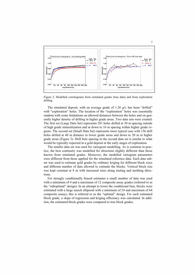
grades from the drill holes has been chosen for this study. Maximum range of gold
continuity is at 160° azimuth and is much shorter in vertical direction and at 70°
azimuth (Figure 2). The relative nugget effect of 25% and ranges of continuity
spanning from 40 to 60 m are quite typical and encountered in many gold depos-
its. Note that although the following analysis is based on simulated grades, con-
sidering a large number of drill holes in a relatively small area from which the
simulated grades are derived, the simulated grades do represent a distribution that
closely resembles actual grades in this deposit.
7
Figure 2: Modelled correlograms from simulated grades (true data) and from exploration
drilling
The simulated deposit, with an average grade of 1.26 g/t, has been “drilled”
with “exploration” holes. The location of the “exploration” holes was essentially
random with some limitations on allowed distances between the holes and on gen-
erally higher density of drilling in higher grade areas. Two data sets were created:
The first set (Large Data Set) represents 281 holes drilled at 30 m spacing outside
of high grade mineralization and at down to 16 m spacing within higher grade re-
gions. The second set (Small Data Set) represents more typical case with 156 drill
holes drilled at 40 m distance in lower grade areas and down to 20 m in higher
grade areas (Figure 3). Drill hole spacing in the second data set is similar to what
would be typically expected in a gold deposit at the early stages of exploration.
The smaller data set was used for variogram modelling. As is common in prac-
tice, the best continuity was modelled for directions slightly different than those
known from simulated grades. Moreover, the modelled variogram parameters
were different from those applied for the simulated reference data. Each data sub-
set was used to estimate gold grades by ordinary kriging for different block sizes
and different number of data allowed to estimate the blocks. Vertical block size
was kept constant at 8 m with increased sizes along easting and northing direc-
tions.
For strongly conditionally biased estimates a small number of data was used
with a minimum of 4 and a maximum of 12 composite assay grades (referred to as
the “suboptimal” design). In an attempt to lower the conditional bias, blocks were
estimated with a large search ellipsoid with a minimum of 24 and maximum of 64
composite assays; this is referred to as the “optimal” design. For each estimated
block grade, a slope of regression and kriging efficiency was calculated. In addi-
tion, the estimated block grades were compared to true block grades.

8
Figure 3: Plan view of true block grades and data locations: (a) large data set; (b) small,
more typical, data set
Results
Figure 4 shows how slope of regression and kriging efficiency change for different
block sizes, different data sets, and estimation parameters used. As discussed,
modification to the estimation parameters was limited to a number of data used
starting from “poorly-designed” not optimal estimation procedure with small
number of data used for the estimation, and ending with “well-designed” optimal
process with large number of data used for the estimation. As expected, the opti-
mal estimation procedure results in higher slope of regression and increases
kriging efficiency.
It is interesting that for the small data set used in the estimation, the actual
block size did not have any effect on the slope of regression and kriging efficien-
cy. On the other hand, when the large data set was used there was gradual increase
in kriging efficiency with the increased block size. Note that kriging efficiency is
quite low regardless of the estimation type. As expected, using the large number
of data (optimal case) to estimate block grades resulted in a substantial increase in
the slope of regression, i.e., it resulted in substantial decrease of conditional bias.
Not surprisingly, the slope of regression is quite high for the large data set and

9
large number of data used for the estimation. These graphs clearly indicate that us-
ing a lot of data during the estimation process lowers conditional bias and increas-
es kriging efficiency.
Now that it has been established that applying more data to the block estimates
increases slope of regression and by extension decreases conditional bias, the next
step involved comparisons of actual true block grades with the estimated grades
for different cut-offs. Figures 5 and 6 show relative tonnage and grade differences
between true and estimated block grades at the 1.0 g/t cut-off for optimal and not
optimal estimates from the small data and the large data sets, respectively. Both
figures show that despite high conditional bias in the suboptimal design, the esti-
mated tonnes and grades are closer to reference tonnage and grade in the deposit.
This is also true for the estimates from the large data set, although here the differ-
ences between the not optimal and optimal models are smaller. Note that, as pre-
sented in Figure 6, at 20 m block size estimated tonnes and grade are very similar
to reference tonnes and grade. At the same time it would be misleading to con-
clude that this block size produced superior estimates.
In fact, the reported tonnage and grade from different block sizes is quite simi-
lar (Figure 7). It just happens that the estimated tonnes and grade in this specific
deposit are comparable to recoverable tonnes and grade at the selective mining
unit (SMU) size higher than 20 m; roughly the size of half of drill hole spacing.
This is an important observation that suggests it does not matter what block size is
used for estimating resources. Reported resource at 8 m or 20 m block size will be
similar, but the 20 m block appears to approach the size that, if successfully ap-
plied during mining operation, would result in actually recovered tonnes and grade
very similar to those estimated. As long as there is no connection made between a
block size used and actual SMU considered for mining there is nothing particular-
ly wrong with estimates based on a small block size.
Figure 4: Slope of regression (a) and kriging efficiency (b) for blocks estimated from two
data sets for different block sizes and different estimation parameters

10
Figure 5: Relative tonnage and grade differences between estimated and true block grades
at 1.0 g/t cut-off. The blocks were estimated from typical, smaller data set.
Figure 6: Relative tonnage and grade differences between estimated and true block grades
at 1.0 g/t cut-off. The blocks were estimated from large data set
An important result of the optimization of the estimation process is high
smoothing of the estimated block grades. The smoothing effect may result in large
differences between estimated and actual metal content at higher cut-off values.
For block estimates from the typical (smaller) data set, the estimated metal content
at higher cut-offs may be as much as 70-80% lower than the actual metal content
(Figure 8) for the ‘optimized’ parameters, while the ‘sub-optimal’ model yields
50-60% less metal content relative to the reference. Similar conclusions can be
made for the larger data set, with percent differences ranging from 20-30% for the
sub-optimal model and 30-50% for the optimal model. Therefore, it is obvious that
the lower the conditional bias the higher the smoothing effect that can be expected
when estimating from sparsely spaced data. The interesting trend, however, is that
for both the sparsely and densely sampled data sets, the sub-optimal set of parame-
ters yield the closest estimate of contained metal for cut-off grades above the 1.25
g/t mean grade.

11
Figure 7: Estimated from small data set grade and proportion of tonnage above 1.0 g/t cut-
off for different block sizes
Figure 8: Relative metal losses in estimated block grade models for different cut-offs in 16
m block models
The final task considered comparison of the estimation models with conditional
simulation of the small data set. The purpose of this exercise was to compare the
estimation model to a model constructed using a method that is considered to
avoid conditional bias altogether (McLennan & Deutsch, 2002) (Journel &
Kyriakidis, 2004). The reference distribution was obtained via p-field simulation
wherein the local distributions of uncertainty considered a local trend model. For
this task, sequential Gaussian simulation was performed with no consideration for
any trends, and variograms were calculated based on the small data set. As with

12
the estimation models, the continuity directions vary slightly from those of the
reference model. Multiple realizations were then generated at a 2x2x2 m resolu-
tion, and subsequently block averaged to various block sizes: 8, 12, 16 and 20 m.
The uncertainty in grades and tonnage at a series of different cut-off grades
were assessed, and the combined impact is summarized as contained metal at dif-
ferent cut-off grades (Figure 9). The corresponding sensitivity curves for the sub-
optimal and optimal estimation models, along with the reference model, are shown
for comparison. Three interesting observations are made. Firstly, at a cut-off grade
up to the mean grade of 1.25 g/t, there is no appreciable difference between the
contained metal estimated using the optimal or sub-optimal parameters. Secondly,
for the four block sizes considered, the sub-optimal parameters yield estimates
closest to the reference model at higher cut-off grades. Thirdly, the simulation ap-
proach, which is considered to be a non-biased method, yields the distributions of
uncertainty in contained metal that encompasses the reference data. This latter ob-
servation is important, particularly as a reference model is never available in prac-
tice for benchmarking purposes. This indicates that a conditional simulation ap-
proach can be used to validate the estimated tonnage, grades and ultimately metal
when determining an appropriate set of estimation parameters.

13
Figure 9: Contained metal curves for estimated block models for different cut-off grades at
8m, 12m, 16m and 20m block sizes.
Discussion
Both slope of regression and kriging efficiency assume global stationarity within a
specifically modelled domain. Mineral deposits are not stationary, even within a
specific estimation domain. In an estimation domain there are always small re-
gions of high and small regions of very low grades. Slope of regression and
kriging efficiency formulas do not take into account the fact that true variance of
estimation errors depends on data values. In regions with higher grade or in re-
gions with local data having more variance than in the whole domain, fluctuation
of errors is larger. Disregarding these local changes in variability may lead to es-
timated resources that steer away from what would be expected of a typical re-
source estimate.

14
A resource block model should not be designed to produce an inventory of re-
coverable resource that is based on SMU size much larger than would generally be
considered for mining, only because for this SMU size, when mined, the resource
model will turn out to be correct. A deposit is never mined according to a resource
block model. A decision on what will be mined will be based on grade control
drilling, necessary both in open pit and underground mining. A resource geologist
should strive to produce a block model that predicts, reasonably well, the tonnage
and grade that a mine can expect to achieve over the life of the mine, once it has
sorted out its grade control procedures. In addition, the resource block models are
often used for dilution calculations, or blending issues. A block model designed
from optimizing slope of regression, or block size will not serve this purpose.
In short, optimizing kriged block estimates with slope of regression or kriging
efficiency measures may lead to block models that do not adequately reflect true
block grades. It is tempting and easy to use slope of regression and kriging effi-
ciency for validation of block estimated grades. Those measures are commonly
available in commercial software packages. Although theoretically high slope of
regression, i.e. low conditional bias, is considered necessary for good quality es-
timates, in practice this approach may be outright harmful if the objective of the
study is to predict global resource quantities above an economic cut-off grade.
Both measures are a reflection of a modelled variogram and data locations and do
not take into account actual assay values, or their variability in the vicinity of an
estimated block. Moreover, it is often quite difficult to construct a reliable vario-
gram model, particularly in early exploration stages, and relying on its metrics to
design “best” resource estimates cannot be considered best practice.
Based on the presented case study, there is strong indication that it is better to
have conditionally biased block estimates for global resource quantities required
for a potential investment decision, life-of-mine planning and/or development de-
cisions. Once a cut-off is applied to block estimated grades for reporting or further
mining studies, it is better to have unsmoothed conditionally biased block esti-
mates. In this context of achieving globally accurate predictions, it looks like the
onus is back on a resource geologist to design estimation parameters that produce
a realistic block model that reflects the underlying true block grades the best way
possible.
Bibliography
Arik, A. (1990). Effects of Search Parameters on Kriged Reserve Estimates.
International Journal of Mining and Geological Engineering, 8(4), 305-
318. Deutsch, J., Szymanski, J., & Deutsch, C. (2014). Checks and Measures of
Performance for Kriging Estimates. Journal of the South African Institute
of Mining and Metallurgy, 223-230.

15
Isaaks, E. (2005). The Kriging Oxymoron: A Conditionally Unbiased and
Accurate Predictor (2nd Edition). Geostatistics Banff 2004 (pp. 363-374).
Dordrecht: Springer.
Journel, A., & Huijbregts, C. (1978). Mining Geostatistics. London: Academic
Press.
Journel, A., & Kyriakidis, P. (2004). Evaluation of Mineral Reserves: A
Simulation Approach. New York: Oxford University Press.
Krige, D. (1997). A practical analysis of the effects of spatial structure and of data
available and accessed, on conditional biases in ordinary kriging.
Geostatistics Wollongong '96, Fifth International Geostatistics Congress
(pp. 799-810). Dordrecht: Kluwer.
Krige, D., Assibey-Bonsu, W., & Tolmay, L. (2005). Post Processing of SK
Estimators and Simulations for Assessment of Recoverable Resources
and Reserves for South African Gold Mines. Geostatistics Banff 2004
(pp. 375-386). Dordrecht: Springer.
McLennan, J., & Deutsch, C. (2002). Conditional Bias of Geostatistical
Simulation for Estimation of Recoverable Reserves. CIM Proceedings
Vancouver 2002. Vancouver: CIM Proceedings Vancouver 2002.
Olea, R. (1991). Geostatistical Glossary and Multilingual Dictionary. New York:
Oxford University Press.
Rivoirard, J. (1987). Teacher's Aide: Two Key Parameters when Choosing the
Kriging Neighborhood. Mathematical Geology, 851-856.
Sinclair, A., & Blackwell, G. (2002). Applied Mineral Inventory Estimation.
Cambridge: Cambridge University Press.
Vann, J., Jackson, S., & Bertoli, O. (2003). Quantitative Kriging Neighbourhood
Analysis for the Mining Geologist - A description of the method with
worked case examples. 5th International Mining Geology Conference,
(pp. 1-9). Bendigo.