Embed Size (px)
Citation preview

Confidence Intervals
List of things to Do:-
• Compute the point estimate of µ
• Compute the confidence intervals about µ with σ known
• Error term in the confidence interval
• Determine the sample size n for estimating the population means
• Explain the meaning of Confidence interval
• SAS command to calculate C.I (Confidence Interval)
1

Basics
• A Population is any entire collection of
people, animals, plants or things from which we
may collect data. It is the entire group we are
interested in, which we wish to describe or draw
conclusions about.
Example:- The population for a study of infant
health might be all children born in the U.K. in the
2000′s.
• A Sample is a group of units selected from a
larger group (the population). By studying the
sample it is hoped to draw valid conclusions about
the larger group.
Example:- The population for a study of infant
health might be all children born in the U.K. in the
1980′s. The sample might be all babies born on 7th
May in any of the years.
2

Basics
• A Parameter is a value, usually unknown (and
which therefore has to be estimated), used to
represent a certain population characteristic.
For example, the population mean is a parameter
that is often used to indicate the average value of a
quantity.
µ represents the population mean.
σ represents the population standard deviation.
p represents the population proportion.
• A Statistic is a quantity that is calculated from a
sample of data. It is used to give information about
unknown values in the corresponding population.
For example, the average of the data in a sample is
used to give information about the overall average
in the population from which that sample was
drawn.
x will estimate µ.
s will estimate σ.p will estimate p.
3

Basics Continued...
About Normal Distribution
A normal distribution with mean µ and variance σ2 is a
statistic distribution with probability function
N(µ, σ) = P (X) =1
σ√
2πe− (x−µ)2
2σ2
where x ∈ (−∞,∞), µ ∈ R and σ ≥ 0 .
While statisticians and mathematicians uniformly use
the term ’Normal Distribution’ for this
distribution, physicists sometimes call it a Gaussian
distribution and, because of its curved flaring shape,
social scientists refer to it as the Bell Curve.’
4

Basics Continued...
Normal to Standard Normal
Let ,
Z =X − µ
σ
N(0, 1) = P (Z) =1√2π
e−Z22
At the back of the book the normal table used is based
on the above formula.
5

Basics Continued...
Finding the Area under theStandard Normal Curve
6

Basics Continued...
Finding the value of Zα
7

Basics Continued...
Binomial to Standard Normal
B(n, p) =
n
x
px(1− p)n−x
where n is the number of trials, r is the number of
success and p is the probability of success.
If np(1− p) ≥ 10, the binomial experiment is
approximately Normal, with mean µ = np and standard
deviation σ =√np(1− p).
Standardize the Binomial random variable X we obtain,
Z =x− µ
σ=
x− np√np(1− p)
8

Point Estimates
Def:- A point estimate of a parameter is the value of a
statistic that estimates the value of the parameter.
Example:- Suppose X1, X2, , X10 are random samples
which follow normal distribution with mean µ and
standard deviation s = 2.5. Hence in this problem the
parameter µ is unknown and we want to estimate µ
from the given 10 samples. In order to understand this
fact more clearly we need following definition:-
Unbiased Estimator:- An estimate s is said to be
an unbiased estimator of the parameter µ if E(S) = µ.
9

Theorem:- Let X1, X2, ..., Xn be the random sample
from the population with mean µ. The sample mean X
is an unbiased estimator for the population mean µ.
Solution:- We have to show that E(X) = µ.
E(X) = E(∑
Xi
n) =
1
nE(
∑Xi) =
1
n
∑E(Xi)
But we know that E(Xi) = µ. Therefore the above
equation boils down to
E(X) =nµ
n= µ.
Note:- From the above proof we observed that X ′is
and X are the unbiased estimators of µ. Which one is
the best one, the X ′is or the X . The answer is X is the
better unbiased estimator, also note that we can find
many unbiased estimators. A good question is which is
the best. The answer to this question is beyond the
reach of this Class.
10

Hence for your example the
X1 + X2 + ... + X10
10= X
estimates µ. Hence the unknown population mean has
been estimated by some known fact. Isn’t it great!!!!!
11

Computing the confidence intervals about µ
with σ known.
Assumption:- The data should be from a normal
population or the sample size is greater than 30. The
way to check the normality of the data if sample size is
less than 30, is to plot the data and see whether it is
approximately a straight line with no outliers. I will
talk about outliers in SAS.
Confidence Interval:- A confidence interval
estimate of a parameter consists of an interval of
numbers, along with the measure of the likelihood that
the interval contains the unknown parameter.
(x− zα2∗ σ√
n, x + zα
2∗ σ√
n)
• x is the point estimate for µ.
• α our level of confidence.
• the standard deviation of the sample mean. (What
represents standard deviation of the sample mean
x?)
C.I can be rewritten as
Point Estimate ± Margin of Error
12

Interpretation of ConfidenceInterval
Let X1,..., Xk denote K samples, each of size n, from a
population with mean µ and standard deviation
σ(Known). Let us construct (1− α)100% C.I for each
of these samples of size n. Let the C.I’s are denoted by
C1,...,Ck. We will observe that, approximately
(1− α)100% of the C.I’s will contain µ.
Suppose k = 20 and α = .10. Suppose 90% confidence
interval for µ is calculated as (25, 36). That means ”we
are 90% confident” that µ lies between 25 and 36. In
other words out of 20 C.I’s approximately 18 of C ′ks will
contain µ.
13

Error term in the confidence interval
The margin of error term in confidence interval is
denoted as E.
E = zα2∗ σ√
n
The error E suggests that if we increase the sample size
then we will expect less error, that means the confidence
interval will become more shallower, hence will be a
good estimator of the unknown population parameter.
Determining the sample size n
The sample size required to estimate the population
mean µ, with a given level of confidence and with a
specified margin of error(or minimum error tolerance) E
is given by
n = (zα
2∗ σ
E)2
14

Miles on Cavalier
A researcher is interested in approximating
the mean number of miles on three-year old
Chevy Cavaliers. She finds a random sample
in Orlando, Florida area and obtained the
following result
37,815 20,000 57,103 46,585 24,822
49,678 30,983 52,969 8,000 39,862
6,000 65,192 34,285 30,906 41,841
39,851 43,000 74,362 52,664 33,587
52,896 45,280 30,000 41,713 76,315
22,442 43,301 52,899 41,526 28,381
55,163 51,812 36,500 31,947 16,529
15

• Obtain a point estimate of the
population mean number of miles on a
three-year old Cavalier.
Ans:- x = 40, 463.11 miles is the point estimate for
population mean. That means we can roughly
claim that a three-year old Cavalier will have
40,463.11 miles on it.
• Construct a 99% confidence interval for
the population mean number of miles on a
three-year old Cavalier assuming that
σ = 16, 100.
Ans:- The 99% confidence interval is given by
(40463.11−z0.012∗ 16100√
35, 40463.11+z0.01
2∗ 16100√
35)
or
(33456.14 , 47469.97).
Hence we are 99% confident that the population
mean number of miles will lie between 33456.14 and
47469.97.
16

• From the above result can we say
something regarding the population mean
number of miles in U.S.A. If not then
how nicely the data describes the mean
population miles for a three-year old
car in an around Florida.
Ans:- No. As this is a local Florida data.
The confidence interval is pretty big. Hence we can
say that this interval is a moderate estimate of the
population mean at 99% level of significance. In
order to estimate the population mean more
accurately we need to look at other factors, like sex,
driving conditions, age group and so on.. .
17

Computing the confidence intervals about µ
with σ uknown.
Assumption:- The data should be from a normal
population or the sample size is greater than 30.
Confidence Interval in this case is given by
(x− tα2∗ s√
n, x + tα
2∗ s√
n)
where t denotes the Student’s-t distribution with n-1
degrees of freedom. Everything remains the same as
above.
18

Using the same data set from the previous
problem Construct a 99% confidence interval
for the population mean number of miles on
a three-year old Cavalier assuming that
σ = unknown.
Ans:- The 99% confidence interval is given by
(40463.11− t0.012∗ s√
35, 40463.11 + t0.01
2∗ s√
35)
= (40463.11−t0.012∗ 16149.65√
35, 40463.11+t0.01
2∗ 16149.65√
35)
(33015.17 , 47911.06).
Hence we are 99% confident that the population mean
number of miles will lie between 33015 and 47911, when
σ is unknown.
19

SAS Program
options linesize=80 nodate; run;
title ’Miles in Three-Year old Chevy Cavalier’;
data Chevy;
input miles;
cards;37815200005710346585248224967830983529698000398626000651923428530906418413985143000743625266433587528964528030000417137631522442433015289941526283815516351812365003194716529 ;
proc print data=Chevy;run;proc means data=chevy;
proc means data=Chevy lclm uclm alpha=0.01 ;VAR miles;run;
20

SAS Output
Miles in Three-Year old Chevy Cavalier in Orlando, Florida
Obs miles1 378152 200003 571034 465855 248226 496787 309838 529699 800010 3986211 600012 6519213 3428514 3090615 4184116 3985117 4300018 7436219 5266420 3358721 5289622 4528023 3000024 4171325 7631526 2244227 4330128 5289929 4152630 2838131 5516332 5181233 3650034 3194735 16529
21

SAS Output Continued...
The MEANS Procedure
N Mean Std Dev Maximum Minimum
35 40463.11 16149.65 6000 76315.00
Lower 99% CL for Mean Upper 99% CL for Mean
33015.17 47911.06
22

Problem on Sample Size Determination
The dean of a college wants to use the mean of a randomsample to estimate the average amount of time students taketo get from one class to the next, and she wants to be able toassert with probability 0.95 that her error will be at most 0.30minute. If she knows from studies of a similar kind that it isreasonable to let σ = 1.50 minute, how large a sample will sheneed?
Ans:- The things that are given to us
• E = 0.30
• σ = 1.50
• z .052 = 1.96
We need to find the sample size n.
n = (zα
2∗ σ
E)2 = (
z 0.052∗ 1.50
0.30)2 = 96.04
23

Computing the confidence intervals about a
Population proportion.
Let p denote the population proportion. The best point
estimate for p is denoted by p.
x
n= p → p
The Confidence Interval in this case is denoted by
(p− zα2∗
√√√√√p(1− p)
n, p + zα
2∗
√√√√√p(1− p)
n)
Determining the Sample size n The sample size
required to obtain a (1− α)%100 confidence interval for
p with a given margin of error E, is given by
n = p(1− p)(zα
2
E)2
24

The Death Penalty(8.3 Problem 21)
In a Harris Poll conducted in July, 2000, 64% of the
people polled answered yes to the following question:
”Do you believe in capital punishment, that is the death
penalty, or are you opposed to it?” The margin of Error
was ±3%, and the estimate was made with 95%
confidence. How many people were surveyed?
Ans:- The things that are given to us
• E = 0.03
• p = 0.64
• z .052
= 1.96
We need to find the sample size n.
n = p(1− p)(zα
2
E)2 = 0.64(1− 0.64)(
1.96
0.03)2 = 983.4
Hence 984 people were surveyed.
25

Computing the confidence intervals about a
Population Variance.
If a random sample of size n is obtained from a
normally distributed population with mean µ and
standard deviation σ, then
χ2 =(n− 1)s2
σ2
has a chi-square distribution with n− 1 degrees of
freedom.
The Confidence Interval about σ2 is given by
((n− 1)s2
χ2α2
,(n− 1)s2
χ21−α
2
)
26

Tests of Hypothesis
List of things to do:-
• Determine the null and alternative hypothesis from
a claim
• Type I and Type II error
• Calculation of Power
27

Basic Definitions:- The Null Hypothesis is,
denoted by H0, is a statement to be tested. The null
hypothesis is assumed to be true until we have evidence
against it.
The Alternative Hypothesis denoted by H1, is a
claim to be tested.
Ways to set up H0 and H1:-
28

Figuring out Null and Alternative Hypothesis
from a given data.
The following data is a survey of 15 Blood pressure
patients before and after taking B.P medication for 6
months.
No. of Observations Before Medication After Medication
1 140 134
2 123 126
3 150 130
4 174 140
5 134 120
6 147 142
7 132 125
8 150 120
9 190 150
10 162 133
11 167 135
12 168 142
13 145 129
14 145 120
15 159 130
29

Let µ0 denote the mean Blood Pressure before taking
Medication.
Let µ1 denote the mean Blood Pressure after taking
Medication.
H0 : µ0 = µ1
H1 : µ0 > µ1
Hence we claim that after taking medication the Blood
Pressure will go down.
30

Different Types of Hypothesis Testing
• Simple vs Simple
Example:-
H0 : µ = 0
H1 : µ = 3
• Simple vs Composite
Example:-
H0 : µ = 0
H1 : µ ≥ 0
• Composite vs Composite
Example:-
H0 : µ < 0
H1 : µ ≥ 0
31

Type I and Type II Error
H0 Is true H1 Is True
Do not Reject H0√
Type II Error
Reject H0 Type I Error√
• Hence a Type I Error would occur if the Null
Hypothesis is Rejected when, in Reality the Null
Hypothesis is True.
• Power of a Hypothesis Test is the Probability of
Rejecting Null Hypothesis when, in reality H0 is
False. Hence its a correct decision.
We are now ready to define the Level of Significance
and Power of a Hypothesis Test.
32

Level of Significance:- The level of Significance, α,
is the probability of making a Type I Error.
α = P (RejectingH0|H0isTrue)
Probability of type II Error:- Probability of Type
II Error is denoted by β and is defined as
β = P (NotRejectingH0 | H1istrue).
Probability of type II Error:-
Remarks:- In problems we fix α, as
.05(95%), .01(99%), .1(90%) . That means we fix the
margin of error and the small it is , the good for the
experiment. In general it is known that Type I error is
more severe than Type II error, hence always want a
small α. On the other hand we will like to get a bigger
Power to decide how powerful the test is.
33

Problem 27. Potato Consumption:- According to
the Statistical Abstract of the United States, the mean
per capita consumption of potatoes in 1999 was 48.3
pounds. A Researcher believes that the potatoes
consumption has risen since then.
1. Determine the Null and the Alternative Hypothesis.
Ans:-
H0 : µ = 48.3
H1 : µ > 48.3
2. Suppose, in reality the mean capita consumption of
potatoes is 48.3 pounds. Was a Type I or Type II
error committed. If we test this hypothesis at the
α = 0.05 level of significance, what is the
probability of committing a Type I error.
Ans:- Hence H0 is true and its rejected, we are
committing a Type I Error. And the Probability of
Type I Error is α = 0.05.
34
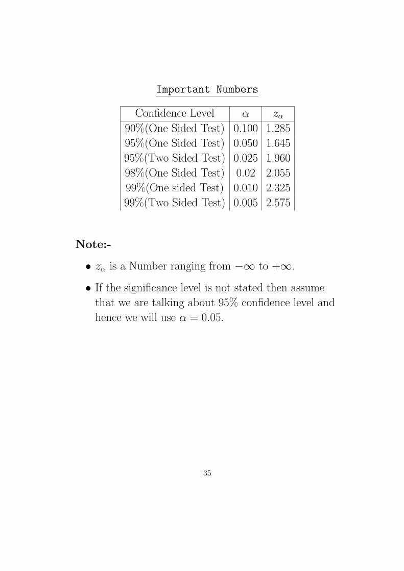
Important Numbers
Confidence Level α zα
90%(One Sided Test) 0.100 1.285
95%(One Sided Test) 0.050 1.645
95%(Two Sided Test) 0.025 1.960
98%(One Sided Test) 0.02 2.055
99%(One sided Test) 0.010 2.325
99%(Two Sided Test) 0.005 2.575
Note:-
• zα is a Number ranging from −∞ to +∞.
• If the significance level is not stated then assume
that we are talking about 95% confidence level and
hence we will use α = 0.05.
35
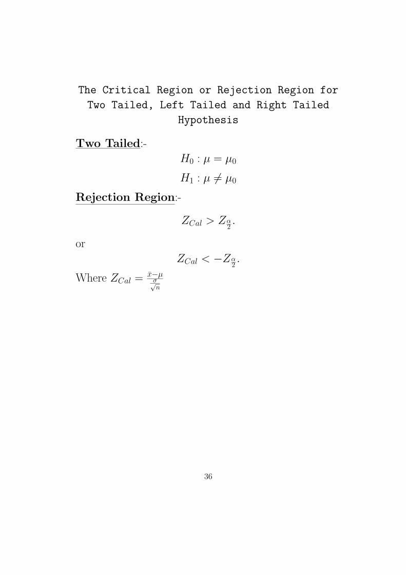
The Critical Region or Rejection Region for
Two Tailed, Left Tailed and Right Tailed
Hypothesis
Two Tailed:-
H0 : µ = µ0
H1 : µ 6= µ0
Rejection Region:-
ZCal > Zα2.
or
ZCal < −Zα2.
Where ZCal = x−µσ√n
36

Left Tailed:-
H0 : µ = µ0
H1 : µ < µ0
Rejection Region:-
ZCal < −Zα.
Where ZCal = x−µσ√n
37

Right Tailed:-
H0 : µ = µ0
H1 : µ > µ0
Rejection Region:-
ZCal > Zα.
Where ZCal = x−µσ√n
38

Problems of Power
For a given population with σ = $12, we want to test
the null hypothesis µ = $75 on the basis of random
sample of size n = 100. If the Null hypothesis is
rejected when x is greater than or equal to $76.50. and
otherwise it is accepted, find
• the probability of Type I error.
Ans:-
α = Probability of Type I Error = P(Reject H0|H0
is True)
The rejection region is given as x ≥ 76.50.
Mathematically,
α = P (x ≥ 76.50 | H0isTrue)
α = P (x ≥ 76.50| µ0 = $75)
α = P (Z = x−µ0σ√n≥ 76.50−µ0
σ√n
) = P (Z ≥ 76.50−7512√100
)
α = P (Z ≥ 76.50−7512√100
) = P (Z ≥ 1.25) = 0.1056
Hence level of confidence is approx. 90%.
39

• The power of the hypothesis when µ0 = 75.30. Is it
a good power?
Ans:-
Power = P(Reject H0|H1 is True)
Mathematically, Power = P (x ≥ 76.50| µ0 = 75.30)
Power = P (Z =x− µ0
σ√n
≥ 76.50− µ0σ√n
)
= P (Z ≥ 76.50− 75.3012√100
)
= P (Z ≥ 76.50− 75.3012√100
)
= P (Z ≥ 1) = 0.1587
Conclusion:- Its a Awful Power. A good Power
should be close to 1. And .1587 is not.
40

• The probability of Type II Error when µ = 77.22.
Is it good?
Ans:-
Power = P(Reject H0|H1 is True)
Mathematically, Power = P (x ≥ 76.50| µ0 = 77.22)
Power = P (Z =x− µ0
σ√n
≥ 76.50− µ0σ√n
)
= P (Z ≥ 76.50− 77.2212√100
)
= P (Z ≥ 76.50− 77.2212√100
)
= P (Z ≥ −0.6) = 0.7257
Conclusion:- Its a Good Power. A good Power
should be close to 1. And .7257 is close to 1.
41

Problem 5, Sec 9.6:- In order to test H0 : µ = 20 v.s
H1 : µ < 20, a simple random sample of size n = 18 is
obtained from a population that is known to be
normally distributed with σ = 3.
• What would it mean to make a Type II Error?
Ans:- A Type II Error would occur if the sample
data led to a conclusion of not rejecting µ = 20
when in fact µ < 20.
42

• If the researcher decides to test this hypothesis at
α = 0.05 level of significance, compute the Power of
the test if the true population mean is 17.4. What
is P(Type II Error)?
Ans:-
Power = P(Reject H0|H1 is True)
Computing The Rejection Region:- Observe
that this is a Left Tailed Test , hence the
rejection region is given in terms of x as follows
x < µ− zασ√n
or
x < 20− 1.6453√18
= 18.84
Power = P(Reject H0|H1 is True)
= P(x < 18.84 | µ = 17.40)
Standardizing we get
= P (Z = x−µ0σ√n≤ 18.84−µ0
σ√n
) = P (Z ≤ 18.84−17.403√18
)
= P (Z ≤ 2.04)
= 0.9793
43

Geometrically:-
44

• Redo part b if the true population mean is 19.2.
45

Problem 12, Sec 9.6:- A school administrator states
that students whose first language learned is not english
do not score differently on the Math portion of the SAT
Exam from students whose first language is English.
The mean SAT math score of students whose first
language is english is 516., according to the data
obtained from the College Board. Suppose the
researcher obtains a simple random sample of 20
students whose first language learned was not english,
SAT math scores are normally distributed with a
population standard standard deviation of 109.
• What would it mean to make a Type II Error?
Ans:- A Type II Error would occur if the sample
data led to a conclusion of not rejecting µ = 516
when in fact µ 6= 516.
46

• If the researcher decides to test this hypothesis at
α = 0.05 level of significance, compute the
Probability of Type II Error if the true population
mean is 505. What is Power of the test?
Ans:-
P(Type II Error) = P(Do Not Reject H0|H1 is True)
Computing The Rejection Region:- Observe that
this is a Two Tailed Test , hence the rejection region
is given in terms of x as follows
x > µ + zα2
σ√n or x < µ− zα
2σ√n
Hence do not reject H0 if , µ− zα2
σ√n < x < µ + zα
2σ√n
or
516− z0.052
109√20
< x < 516 + z0.052
109√20
516− 1.96 109√20
< x < 516 + 1.96 109√20
Hence D not reject Reject H0 if x lies (468.23, 563.77).
47

P(Type II Error) = P(Do Not Reject H0|H1 is True)
= P(468.23 < x < 563.77|µ = 505)
Standardizing we get..
= P (468.23−505109√
20< Z < 563.77−505
109√20
)
= P (−1.51 < Z < 2.41)
= .9920− 0.0655 = 0.9265 = β
Hence the Power of this Two Tailed Test is
1− .9265 = 0.0735. Which is a Bad Power.
48

The Classical method of Testing Hypothesis
about µ, σ known
Steps used in Classical method of Testing Hypothesis
about µ, σ known...
Step 1 Figuring out the Null and Alternative
Hypothesis.
Step 2 Write down α value given in the problem and
find the Critical Value Ztab, zα or zα2
depending on
the nature of the test. Also Draw the rejection
region or the critical region.
Step 3 Compute the test Statistic
Z = ZCal =x− µ
σ√n
Step 4 Compare the critical value from the test
Statistic. In other words compare ZCal with Ztab.
Step 5 State the conclusion.
Note:- The procedure presented requires that the data
comes from a population that is Normally distributed or
the sample size is more that 30.
49

Problem 12, Sec 9.2:- A school administrator states
that students whose first language learned is not english
do not score differently on the Math portion of the SAT
Exam from students whose first language is English.
The mean SAT math score of students whose first
language is english is 516., according to the data
obtained from the College Board. Suppose a simple
random sample of 20 students whose first language
learned was not english, results in a sample mean SAT
math score of 518. SAT math scores are normally
distributed with a population standard standard
deviation of 109.
• Why it is necessary for SAT math scores to be
normally distributed in order to test the claim using
the Steps?
Ans:- Since the sample size is less than 20, we need
the SAT math scores to be Normally distributed.
50

• Test the Researcher’s claim using the Classical
Approach at the α = 0.10 level of significance.
Ans:-
The Classical Approach
Step 1
H0 : µ = 516
H1 : µ 6= 516
Step 2 α = 0.10. As this is a two tailed test the
rejection region is given as Z ≥ Zα2
= 1.645 or
Z ≤ −Zα2
= −1.645. Geometrically
Step 3 The Test Statistic
ZCal =x− µ
σ√n
=518− 516
109√20
= 0.08
Step 4 As the test statistic ZCal doesn’t lie in the
critical region, we do not reject the Null
Hypothesis.
Step 5 Hence there is not enough evidence to
support the claim that the mean SAT math
score of Students whose first language is not
english is different from 516.
51

Testing a Hypothesis about µ, σ known,
p- Value Approach
Steps used in Testing Hypothesis about µ, σ known,
p-value approach...
Step 1 Figuring out the Null and Alternative
Hypothesis.
Step 2 Compute the test Statistic
Z = ZCal =x− µ
σ√n
Step 3 Determine the p- value.
For Two tailed test the P-Value is
2P (Z > |ZCal|).For Left tailed test the P-Value is P (Z < ZCal).
For Right tailed test the P-Value is
P (Z > ZCal).
Step 4 Reject the Null Hypothesis if the P-Value is
less than the level of Significance α.
Step 5 State the conclusion.
52
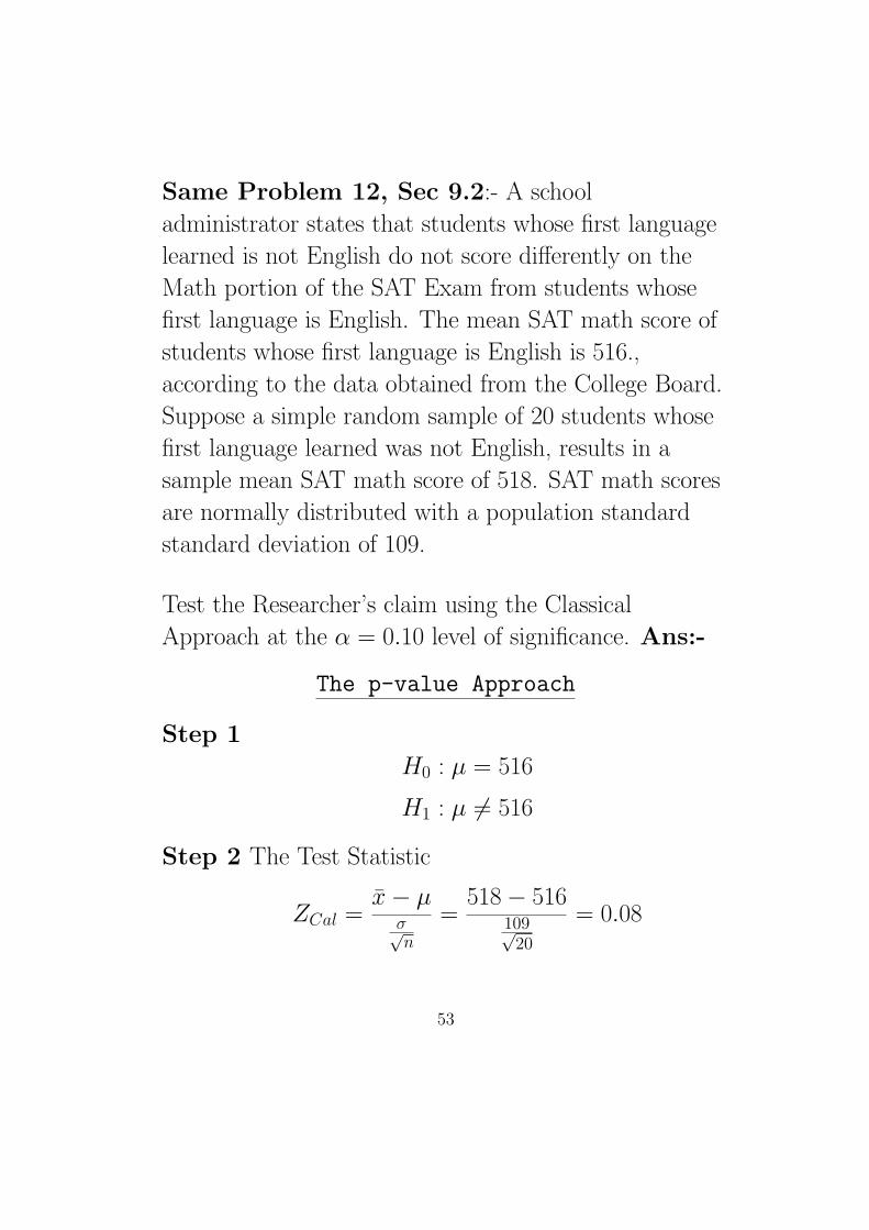
Same Problem 12, Sec 9.2:- A school
administrator states that students whose first language
learned is not English do not score differently on the
Math portion of the SAT Exam from students whose
first language is English. The mean SAT math score of
students whose first language is English is 516.,
according to the data obtained from the College Board.
Suppose a simple random sample of 20 students whose
first language learned was not English, results in a
sample mean SAT math score of 518. SAT math scores
are normally distributed with a population standard
standard deviation of 109.
Test the Researcher’s claim using the Classical
Approach at the α = 0.10 level of significance. Ans:-
The p-value Approach
Step 1
H0 : µ = 516
H1 : µ 6= 516
Step 2 The Test Statistic
ZCal =x− µ
σ√n
=518− 516
109√20
= 0.08
53

Step 3 p- Value is 2P (Z > |0.08|) = 2P (Z > 0.08) =
2(1− 0.5319) = 2(0.4681) = 0.9362
Step 4 As the test statistic p-value is not less than
α = 0.05, we do not reject the Null Hypothesis.
Step 5 Hence there is not enough evidence to
support the claim that the mean SAT math score of
Students whose first language is not English is
different from 516.
54

T Test
The Classical method of Testing Hypothesis
about µ, σ unknown
Steps used in Classical method of Testing Hypothesis
about µ, σ unknown...
Step 1 Figuring out the Null and Alternative
Hypothesis.
Step 2 Write down α value given in the problem and
find the Critical Value ttab, tα or tα2
and also
mention the degrees of freedom. Also Draw the
rejection region or the critical region.
Step 3 Compute the test Statistic
t = tCal =x− µ
s√n
Step 4 Compare the critical value from the test
Statistic. In other words compare tCal with ttab.
Step 5 State the conclusion.
Note:- The procedure presented requires that the data
comes from a population that is Normally distributed or
the sample size is more that 30.
55

Testing a Hypothesis about µ, σ unknown,
p- Value Approach
Steps used in Testing Hypothesis about µ, σ unknown,
p-value approach...
Step 1 Figuring out the Null and Alternative
Hypothesis.
Step 2 Compute the test Statistic
t = tCal =x− µ
s√n
Step 3 Determine the p- value.
Step 4 Reject the Null Hypothesis if the P-Value is
less than the level of Significance α.
Step 5 State the conclusion.
56

Problem 15, Sec 9.3:- In 1989, the average age of an
inmate on a death row was 36.2 years of age, according
to the data obtained from U.S Department of justice. A
sociologist wants to test the Claim that the
average age of a death row inmate has
changed since then. She randomly selects 32 death
row inmates and finds that there mean age is 38.9,
with a standard deviation of 9.6.
• Using the Classical approach test the sociologist’s
claim at the α = 0.05 level of significance.
Ans:-
Step 1
H0 : µ = 36.2
H1 : µ 6= 36.2
Step 2 This is a two sided test, with 31 df and so
the critical values are ±t0.025 = ±2.040.
57

Step 3
t = tCal =x− µ
s√n
=38.9− 36.2
9.6√32
= 1.591
.
Step 4 1.591 doesn’t lie in the critical region,
hence we will not reject the NULL
HYPOTHESIS.
Step 5 Hence there is not enough evidence to
support the claim that the mean age of death
-row inmates is different from 36.2 years.
58

• Determine and Interpret the P-value.
Ans:-
How to find the P value from given tCal
and df?
59

Solution to Problem 20, Sec 9.3:-
Step 1
H0 : µ = 1.62
H1 : µ < 1.62
Step 2 This is a one sided test, with 11 df and so the
critical values are −t0.10 = −1.363.
Step 3
t = tCal =x− µ
s√n
=1.6141− 1.62
0.0053√12
= −3.856
.
Step 4 -1.363 lie in the critical region, hence we reject
the NULL HYPOTHESIS.
Step 5 Hence there is enough evidence to support the
claim that the mean wt of Maxfli XS Golf balls is
less than 1.62 ounces.
60

Determine and Interpret the P-value.
Ans:-
How to find the P value from given tCal and
df?
61

The Classical method of Testing Hypothesis
about population proportion
Steps used in Classical method of Testing Hypothesis
about population proportion
Step 1 Figuring out the Null and Alternative
Hypothesis.
Step 2 Write down α value given in the problem and
find the Critical Value Ztab, zα or zα2
depending on
the nature of the test. Also Draw the rejection
region or the critical region.
Step 3 Compute the test Statistic
Z = ZCal =p− p0√p0(1−p0)
n
Where p is the sample Proportion.
Step 4 Compare the critical value from the test
Statistic. In other words compare ZCal with Ztab.
Step 5 State the conclusion.
Note:- For Normality you should check np0(1− p0) ≥ 10
62

Solution to Problem 12, Sec 9.4:-
Step 1
H0 : p0 = 0.249
H1 : p0 < 0.249
Note:-
np0(1− p0) = 150 ∗ 0.249(1− 0.249) = 28 ≥ 10,
hence the normality requirement is fulfilled.
Step 2 α = 0.05. As this is a Left tailed test the
rejection region is given as Z ≤ −Zα = −1.645.
From the Survey, p = 28150 = 0.187
Step 3 The Test Statistic
ZCal =p− p0√p0(1−p0)
n
=0.187− 0.249√
0.249(1−0.249)150
= −1.76
Step 4 As the test statistic ZCal lies in the critical
region, we reject the Null Hypothesis.
Step 5 Hence there is enough evidence to support
the claim that the percentage of 30-40 year old male
who do not exercise has decreased from its 1998
level.
63

Inference on Two Samples
• Paired Tests(Dependent Samples).
• Welch’s t test(Independent Samples).
• Pooled Two sample t test.
• F Test
64

Paired Tests(Dependent Samples).
Definition:- The sampling method is dependent
when the individuals selected in one sample are used to
determine the individuals to be in the second sample.
As an example we use Paired T test, when, Before and
After kinds of comparison, the ages of Husbands and
wives, first half and second half of the exam, cars
stocked and sold by used car dealers, and numerous
other kinds of situations in which data are naturally
Paired. Steps..
Assumptions:-
1.The sample is obtained using simple random sampling.
2.the sample data are paired.
3. the differences are normally distributed or , the
sample size is greater than 30.
Step 1 Figuring out the Null and Alternative
Hypothesis.
Step 2 Write down α value given in the problem and
find the Critical Value ttab, tα or tα2
and also
mention the degrees of freedom. Also Draw the
rejection region or the critical region.
65

Step 3 Compute the test Statistic
t = tCal =d− 0
sd√n
=dsd√n
Step 4 Compare the critical value with the test
Statistic. In other words compare tCal with ttab.
Step 5 State the conclusion.
Confidence Intervals
A (1− α).100% confidence interval for µd is given by
(d− tα2.sd√n, d + tα
2.sd√n
)
66

Problem 8, Sec 10.1:-Observations 1 2 3 4 5 6 7 8
X1 19.4 18.3 22.1 20.7 19.2 11.8 20.1 18.6
X2 19.8 16.8 21.1 22.0 21.5 18.7 15.0 23.9
1. Determine di = X1 −X2.
Ans:-
X1 X2 X1 −X2
19.4 19.9 -0.4
18.3 16.8 1.5
22.1 21.1 1.0
20.7 22.0 -1.3
19.2 21.5 -2.3
11.8 18.7 -6.9
20.1 15.0 5.1
18.6 23.9 -5.3
2. Compute d and sd.
Ans:-
options linesize=80 nodate; run;
data pair;
infile ’path’
input chaos;
proc means data=pair ;
var chaos;
run;
67

Output
3. Test the claim that µd 6= 0 at the α = 0.01 level of
significance.
4. Compute the 99% confidence Interval about the
population mean difference µd = µ1 − µ2.
68

Welch’s t test(Independent Samples).
Definition:- The sampling method is independent
when the individuals selected in one sample do not
dictate which individuals are to be in the second sample.
Assumptions:-
1.The sample is obtained using simple random sampling.
2.the samples are independent.
3. the population from which the samples are drawn are
normally distributed or the sample sizes are greater
than 30.
Step 1 Figuring out the Null and Alternative
Hypothesis.
Step 2 Write down α value given in the problem and
find the Critical Value ttab, tα or tα2
and the degrees
of freedom will be smaller of n1 − 1 or n2 − 1. Also
Draw the rejection region or the critical region.
Step 3 Compute the test Statistic
t = tCal =(x1 − x2)− (µ1 − µ2)√
s12
n1+ s22
n2
Step 4 Compare the critical value with the test
Statistic. In other words compare tCal with ttab.
Step 5 State the conclusion.
69

Improving the Conservative df of Welch’s t
test
The Welch’s t test is conservative, in order to get
accurate answer we should use
df =(s1
2
n1+ s2
2
n2)2
(s12n1
)2
n1−1 +(s22n2
)2
n2−2
Software will use this particular formula for more
accurate answer.
70

Confidence Intervals about the difference of
two means
A (1− α).100% confidence interval for µd is given by
(x1 − x2)± tα2∗
√√√√√s12
n1+
s22
n2.
where tα2
is obtained using smaller of n1 − 1 or n2 − 1
degrees of freedom or the improved formula.
71

Problem 9, Sec 10.2:- An engineer wanted to know
whether the strength of two different concentrate mix
designs differed significantly. He randomly selected 9
cylinders, measuring 6 inches in diameter and 12 inches
in height, into which mixture 67-0-301 was poured.
After 28 days, he measured the strength(in pounds per
square inch) of the cylinder. He also randomly selected
10 cylinders of mixture 67-0-400 and performed the
same test. the results are as follows:-
Mixture 67-0-301 Mixture 67-0-400
3960 4070
4090 4890
3100 5020
3830 4330
3200 4640
3780 5220
4080 4190
4040 3730
2940 4120
— 4620
1. The data are obtained from simple random sample
that are independent.
2. test the claim that mixture 67-0-400 is stronger
than 67-0-301 at α = 0.05 level of significance.
72

Ans:-
Step 1
H0 : µ400 = µ301
H1 : µ400 > µ301
µ400 = Mean strength of mixture 67-0-400 .
µ400 = Mean strength of mixture 67-0-301 .
Step 2 This is a right tailed test. df = min{9, 8}.tcri = 1.860. Hence Reject H0 if ttab > 1.860.
Step 3 x400 = 4483, n400 = 10
x301 = 3669, n301 = 9
t = tCal =(x400 − x301)− (µ400 − µ301)√
s2400
n400+
s2301
n301
= 3.8
Step 4 As 3.8 > 1.860 , we reject H0.
Step 5 Hence there is enough evidence to conclude
that the mixture 67-0-400 is stronger than
67-0-301.
73

3. Construct a 90% confidence interval about
µ400 − µ301, and interpret the result.
Ans:- The confidence interval is given by
(x400 − x301)± tα2∗
√√√√√√s2400
n400+
s2301
n301.
= 814± 398
= (416, 1212)
We are 90% confident that the the true mean
difference is between 416 and 1212.
74

Pooled Two sample t test.
Pooled t-test is used for independent sample case and it
assumes equal population variance. While Welch’s t-test
doesn’t assume any thing about the population variance.
Comparison between Welch’s t-test and Pooled t-test,
Pooled t-test
Assumes that population variance is same
df = n1 + n2 − 2
t = tCal = (x1−x2)−(µ1−µ2)
sp
√1n1
+ 1n2
where sp =√
(n1−1)s21+(n2−1)s2
2n1+n2−2
Not conservative as compared to Welch’s t-test
P(Type II Error) is normally not so high as
Welch’s t-test
Disadvantage is how to find out the fact that the
population variance are the same? The answer is F-Test which
we will learn later in this section.
75

Problems of Pooled t-test
The following random samples are measurements of the
heat-producing capacity (in millions per calories of tons)
of coal from two mines:-
Mine 1:- 8380 8180 8500 7840 7990
Mine 2:- 7660 7510 7910 8070 7790
Use the 0.05 level of significance to test wether the
difference between the means of these two samples is
significant, assuming that σ1 = σ2.
Ans:-
Step 1
H0 : µ1 = µ2
H1 : µ1 6= µ2
Step 2 α = 0.05, df = n1 + n2 − 2 = 8, Reject H0 if
|tcal| > tcri = 2.306.
Step 3 x1 = 8178, s1 = 271.1,x2 = 7788, s2 = 216.8.
sp =
√√√√√√(n1 − 1)s21 + (n2 − 1)s2
2
n1 + n2 − 2= 245.5
76

tCal =(x1 − x2)
sp
√1n1
+ 1n2
= 2.51
Step 4 As 2.51 > 2.306, we Reject the Null
Hypothesis.
Step 5 Hence there is enough evidence to conclude
that the difference between the two sample mean is
significant.
77

Inference about Two Sample Population
Standard Deviation
When to decide that the population
Variances are Equal?
In order to answer this question we need the following
assumption:-
• The samples are independent simple random
samples.
• The population from which the samples are drawn
must be normally distributed.
78

Introduction of Fisher’s F-distribution
If σ21 = σ2
2 and s21 and s2
2 are sample variances from
independent simple random samples of size n1 and n2
respectively, drawn from normal populations, then
F =s2
1
s22
follows F-Distribution with n1 − 1 numerator degrees of
freedom and n2 − 1 denominator degrees of freedom.
About critical values of F-Distribution:-
79

Steps for Hypothesis Tests on Two
Population Standard Deviation
Step 1 Figuring out the Null and Alternative
Hypothesis.
Step 2 Write down α value given in the problem and
find the Critical Value Fcri as follows:-
• Two Tailed
Fcri = F1−α2 ,n1−1,n2−1 and Fcri = Fα
2 ,n1−1,n2−1.
• Left Tailed
Fcri = F1−α,n1−1,n2−1.
• Right Tailed
Fcri = Fα,n1−1,n2−1.
80

Step 3
Fcal =s2
1
s22
Step 4 Fcal lies in the critical region or not?
Step 5 State the conclusion.
81

Calculate F0.975,12,14
82

Problem 11, Sec 10.4:-
Sample for population 1 Sample for Population 2
n 26 19
s 9.9 6.4
Test the claim that σ1 > σ2 at α = 0.01 level of
significance for the given sample data.
Ans:-
Step 1
H0 : σ1 = σ2
H1 : σ1 > σ2
Step 2 α = 0.01. Right tailed test. Therefore
Fcri = F0.01,26−1,19−1 = F0.01,25,18 = 2.84. Reject H0
if Fcal > 2.84.
Step 3
Fcal =s2
1
s22
=9.92
6.42= 2.39
Step 4 As Fcal is not in the critical region , we do not
reject H0.
Step 5 There is not enough evidence to support the
claim that σ1 > σ2.
83

χ2 Goodness of fit Test
Definition:- A goodness-of-fit test is an
inferential procedure used to determine whether a
frequency distribution follows a claimed distribution.
In other words A statistical test in which the validity of
one hypothesis is tested without specification of an
alternative hypothesis is called a goodness-of-fit
test.The idea behind the chi-square goodness-of-fit test
is to see if the sample comes from the population with
the claimed distribution. Another way of looking at
that is to ask if the frequency distribution fits a
specific pattern.
Two values are involved, an observed value, which is
the frequency of a category from a sample, and the
other is expected frequency, which is calculated based
upon the claimed distribution.( Sometimes know as
expected counts Ei = npi)
The idea is that if the observed frequency is
really close to the claimed (expected)
frequency, then the square of the deviations will be
small. The square of the deviation is divided by the
expected frequency to weight frequencies.
84

The test statistics
χ2 =∑ (Oi − Ei)
2
Eii = 1, 2, ..., k
approximately follows a Chi-Square Distribution with
n− 1 degrees of freedom if the following assumptions
are met.
• The data are obtained from a random sample.
• All expected frequency must be at least 1.
• At most 20% of the expected frequencies are less
than 5.
The following are properties of the
goodness-of-fit test
1. The data are the observed frequencies. This means
that there is only one data value for each category.
2. The degrees of freedom is one less than the number
of categories, not one less than the sample size.
3. It is always a right tail test.
4. It has a chi-square distribution. The value of the
test statistic doesn’t change if the order of the
categories is switched.
85

Steps for Testing A Claim Using a
Goodness-of-Fit Test:-
Step 1 A claim is made regarding a distribution. The
claim is used to determine Null and Alternative
Hypothesis.
H0: The random variable follows the claimed
distribution.
Step 2 Calculate the Expected frequency for each of
the K categories.
Step 3 Verify the assumptions for goodness -of- fit
Test.
Step 4 Compute the test Statistic
χ2Cal =
∑ (Oi − Ei)2
Ei.
Step 5 Find χ2cri = χ2
α with k − 1 degrees of
freedom.
Step 6 Reject H0 if χ2cal > χ2
cri.
Step 7 State the conclusion.
86

Bicycle Deaths:- A researcher wanted to determine
whether bicycle deaths were uniformly distributed over
the days of the week. She randomly selected 200 deaths
that involved a bicycle, recorded the day of the week on
which the day occurred, and obtained the following
results:
Day of week Frequency
Sunday 16
Monday 35
Tuesday 16
Wednesday 28
Thursday 34
Friday 41
Saturday 30
Is there reason to believe that the day of the week on
which a fatality occurs on a bicycle occurs with equal
frequency at the α = 0.05 level of significance?
Ans:-
Step 1
H0 : p1 = p2 = p3 = p4 = p5 = p6 = p7 =1
7
H0: at least one of the pi will is different from 17.
87

Step 2,3,4 will follow from the following diagram.
Observed Count(Oi) Expected Count(Ei) (Oi − Ei)2 (Oi−Ei)
2
Ei
16 200(17) = 28.57
35 28.57
16 28.57
28 28.57
34 28.57
41 28.57
30 28.57
Step 5 df = 7− 1 = 6, χ20.05 = 12.592
88

Problems of χ2 Goodness of fit Test
1. H0 : The random variable X is binomial with
n = 4, p = 0.3.
H1 : The random variable X is not binomial with n = 4,
p = 0.3.X 0 1 2 4 5
Observed 260 400 280 50 10
• Find the Expected Frequency.
• Determine the χ2 test Statistic.
• Determine the degrees of freedom.
• Test the hypothesis at the α = 0.05 level of
significance.
89

Problems of χ2 Goodness of fit Test
2.According to the manufacturer of M&Ms, 30% of
the plain M&Ms in a bag should be brown, 20%
yellow, 20% red, 10% orange, 10% blue, 10% green. A
student wanted to determine whether a randomly
selected bag of plain M&Ms had contents that followed
this distribution. He counted the number of M&Ms
that were colored and obtained the following results.Color Frequency
Brown 125
Yellow 77
Red 90
Blue 31
Orange 42
Green 35Test the claim that plain M&Ms follow the
distribution stated by manufacturer of M&Ms at 0.05
level of significance.
90

Problems of χ2 Goodness of fit Test
3.Number of Radio Messages Observed Frequency
0 70
1 57
2 46
3 20
4 5
5 2
Number of Radio Messages Expected Frequency
0 44.6
1 66.9
2 50.2
3 25.1
4 or more 13.1
Note:- The expected frequency table was
constructed using Poisson Distribution with
λ = 1.5.
H0 : The population sampled has the Poisson
distribution with λ = 1.5.
Test the claim at 0.01 level of significance.
91

Curve Fitting
Model : Yi = β0 + β1Xi + εi
Where
1.Xi is the independent variable (predictor variable)
2.Yi is the dependent variable or (response variable)
3. β1 is the slope and β0 is the Y-intercept.
4. εi is the Error term which follows N(0, σ2).
This model is a population (notice the Greek β′s and ε
known as estimators) simple (meaning one X variable)
linear (meaning straight line) regression model.
If we take the expected value (average) of the
Regression model it becomes E(Yi) = β0 + β1Xi.
(1) The disappears because E(εi) = 0, that is we expect
our error to be zero.
(2) This model indicates that given a level of Xi , you
can generate the mean of the probability distribution of
the Y ′i s at that Xi level.
92

We must estimate the population Regression
line using sample data.
The equation of the Least-squares Regression Line is
given by
Yi = b1x + b0
b1 and b0 are the estimates for β1 and β0 respectively.
We can calculate b1 and b0 from Normal equations.
(”y-hat” is the Predicted Value for any given x.)
Normal Equations
∑y = nb0 + b1
∑x∑
xy = b0∑
x + b1∑
x2
where∑
means summing over all the data points.
Solving the above Normal equations we obtained b1 and
b0 as follows.
b1 =∑
xy − 1n(
∑x)(
∑y)∑
x2 − 1n(
∑x)2
=Sxy
Sxx
b0 =∑
y − b1(∑
x)
n
93

Where
Sxx =∑
x2 − 1
n(∑
x)2
is the variance of observed x′is multiplied by the factor
n− 1.
We will use similar notations later on like
Syy =∑
y2 − 1
n(∑
y)2
is the variance of observed y′is multiplied by the factor
n− 1.
A few more Notations...
Standard Deviation of x′is is denoted by sx =√
Sxxn−1.
Standard Deviation of y′is is denoted by sy =√
Syy
n−1.
94
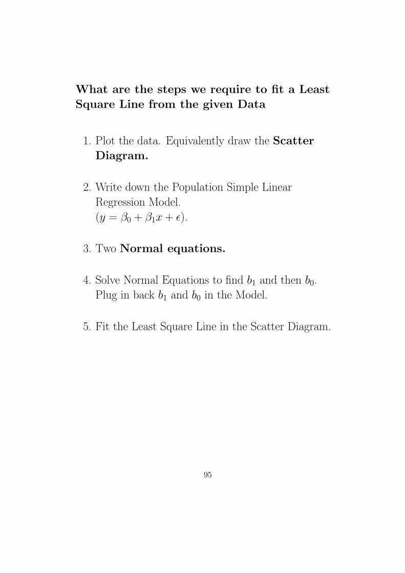
What are the steps we require to fit a Least
Square Line from the given Data
1. Plot the data. Equivalently draw the Scatter
Diagram.
2. Write down the Population Simple Linear
Regression Model.
(y = β0 + β1x + ε).
3. Two Normal equations.
4. Solve Normal Equations to find b1 and then b0.
Plug in back b1 and b0 in the Model.
5. Fit the Least Square Line in the Scatter Diagram.
95

Problems on Curve Fitting
Number of weeks Hearing Range
x y
47 15.1
56 14.1
116 13.2
178 12.7
19 14.6
75 13.8
160 11.9
31 14.8
12 15.3
164 12.6
43 14.7
74 14.0
Here x is the length of time that a person has been
living near a major airport directly in the flight path of
departing jets, and y is his or her hearing range(in
thousands of cycles per second)
Solution:- Solved in the class.
96

Multiple regression
Model:- Y = β0 + β1X1 + β2X2 + ε
The least square multiple regression line is
Y = b0 + b1X1 + b2X2
The normal equations from which b0, b1, b2 are obtained
are,
∑y = nb0 + b1
∑x1 + b2
∑x2∑
yx1 = b0∑
x1 + b1∑
x21 + b2
∑x1x2∑
yx2 = b0∑
x2 + b1∑
x1x2 + b2∑
x22
97
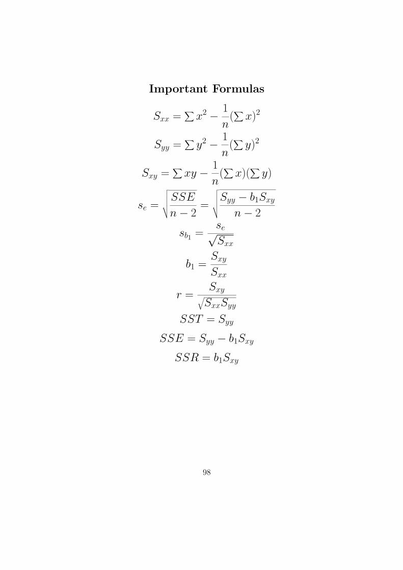
Important Formulas
Sxx =∑
x2 − 1
n(∑
x)2
Syy =∑
y2 − 1
n(∑
y)2
Sxy =∑
xy − 1
n(∑
x)(∑
y)
se =
√√√√√ SSE
n− 2=
√√√√√Syy − b1Sxy
n− 2
sb1 =se√Sxx
b1 =Sxy
Sxx
r =Sxy√
SxxSyy
SST = Syy
SSE = Syy − b1Sxy
SSR = b1Sxy
98

ANALYSIS OF VARIANCE
Motivation:- Suppose we are asked to compare the
cleansing action on the basis of following whiteness
reading of three Detergents on 15 dinner plates. The
data is listed below.
Detergent X 77 81 71 76 80
Detergent Y 72 58 74 66 70
Detergent Z 76 85 82 80 77
Other factors at the time of washing the
dinner plates :-
• how dirty the plates were?
• washing time?
• water temperature and hardness while cleaning.
• what kind of instrument used for washing?
If we calculate the means of whiteness reading we will
have 77 for detergent X, 68 for detergent Y, 80 for
detergent Z.
Remember that a significant test may show
that the differences between sample means
are too large to be attributed to chance,
99

but cannot say why the differences
occurred?
Hence we should introduce a Controlled Experiment
procedure , where every above factors remain the
same during the washing process. That means same
washing time, same dirty ness, use water of exactly the
same temperature and hardness , inspecting the
instrument after each use and so many other factors... .
Isn’t the above Controlled Experiment
tedious?
Ans:-
So what we do to get rid of this Controlled Factors?
We can conduct an experiment in which none of these
factors is controlled , but in which we protect ourselves
against their effect by RANDOMIZATION. That is
we design, or plan, the experiment in such a way that
the variation caused by these factors can be combined
under the general heading of ”Chance”.
Mathematically what we do?
Def:- An analysis of variance expresses a measure
of the total variation in a set of data as a sum of terms,
each attributed to a specific source, or cause, of
variation.
100

The Assumptions of Analysis of Variance
1. Treatment effects are additive.
2. Experimental errors - are random.
3. Experimental errors are independently distributed.
4. Experimental errors follow a normal distribution.
5. Experimental errors have mean zero and constant
variance.
101

Source
Treatment 1 x11 x12 x13 ... x1n
Treatment 2 x21 x22 x23 ... x2n
... ... ... ... ... ...
Treatment K xK1 xK2 xK3 ... xKn
notations:-
Sample in ith row and jth coloumn = xij
Treatment K variance = s2i
Grand Mean = x =x11 + x12 + ... + xKn
Kn
Mean Treatment 1 = x1 =x11 + x12 + ... + x1n
n
Mean Treatment 2 = x2 =x21 + x22 + ... + x2n
n.
.
Mean Treatment K = xk =xk1 + xk2 + ... + xkn
n
102

SST = SS(Tr) + SSE
Equivalently we can re-write the above equations;
SST = SSB + SSW
Mathematically
SST =∑ ∑
(xij − x)2
SSB = n∑
(xi − x)2
SSW =∑ ∑
(xij − xi)2 = (n− 1)(s2
1 + s22 + ... + s2
K)
103

Test H0 : µ1 = µ2 = µ3 = ... = µK
AnOVA TABLE
Source DF Sum of Squares Mean Square F
Treatments K-1 SSB MSB = SSBK−1 F = MSB
MSW
Error K(n-1) SSW MSW = SSWK(n−1)
Total nK-1 SST
note:- This AnOVA works when each Treatment have
same number of observations. The Formulas for SSB,
and SSW will slightly change when we have different
observations in each treatments.
104

COMPUTInG FORMULAS FOR SUM OF
SQUARES (Equal Sample Size)
T = x11 + x12 + ... + xKn
Ti = xi1 + xi2 + ... + xin
SST =∑ ∑
x2ij − 1
KnT 2
SSB = 1n
∑Ti
2 − 1KnT 2
SSW = SST − SSB
105
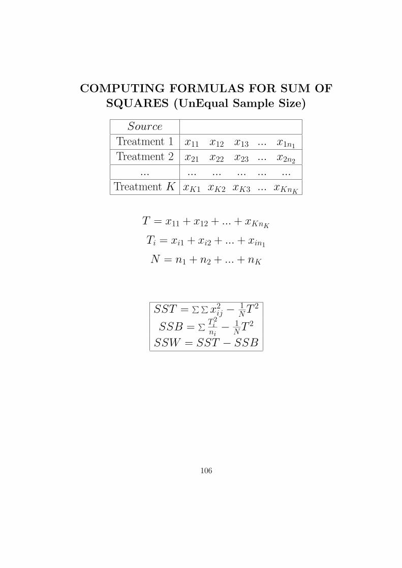
COMPUTING FORMULAS FOR SUM OF
SQUARES (UnEqual Sample Size)
Source
Treatment 1 x11 x12 x13 ... x1n1
Treatment 2 x21 x22 x23 ... x2n2
... ... ... ... ... ...
Treatment K xK1 xK2 xK3 ... xKnK
T = x11 + x12 + ... + xKnK
Ti = xi1 + xi2 + ... + xin1
N = n1 + n2 + ... + nK
SST =∑ ∑
x2ij − 1
N T 2
SSB =∑ T 2
ini− 1
N T 2
SSW = SST − SSB
106

WILCOXON SIGNED RANK TEST FORDEPENDENT SAMPLES (Small (n ≤ 30))
Null Hypothesis H0 : MD = 0 H0 : MD = 0 H0 : MD = 0Alternate Hypothesis H0 : MD 6= 0 H0 : MD > 0 H0 : MD < 0
Test Statistic Smaller(T−, T+) T− T+
Rejection Region T ≤ T0 T− ≤ T0 T+ ≤ T0
1. T− = Sum of Ranks of all negative differences.
2. T+ = Sum of Ranks of all positive differences.
3. T0 = Critical Value.
WILCOXON SIGNED RANK TEST FORDEPENDENT SAMPLES (Large(n > 30))
Null Hypothesis H0 : MD = 0 H0 : MD = 0 H0 : MD = 0Alternate Hypothesis H0 : MD 6= 0 H0 : MD > 0 H0 : MD < 0
Test Statistic zcal zcal zcal
Rejection Region |z| > zα2
z < −zα z > zα
Where T+ is sum of Ranks of all positive differences.
z =T+ − n(n+1)
4√n(n+1)(2n+1)
24
107

Problem WILCOXON SIGNED RANK TEST FORDEPENDENT SAMPLES (Small (n ≤ 30))
A B A-B |A−B| Dummy Ranking Ranking
7 9
4 5
8 8
9 8
3 6
6 10
8 9
10 8
9 4
5 9
108

COMPARING TWO POPULATIONINDEPENDENT SAMPLES
orWILCOXON RANK SUM TEST
(SMALL(n1 ≤ 20 , n2 ≤ 20))
Location 1:- 0.37 0.70 0.75 0.30 0.45 0.16 0.62 0.73
0.33
Location 2:- 0.86 0.55 0.80 0.42 0.97 0.84 0.24 0.51
x
109
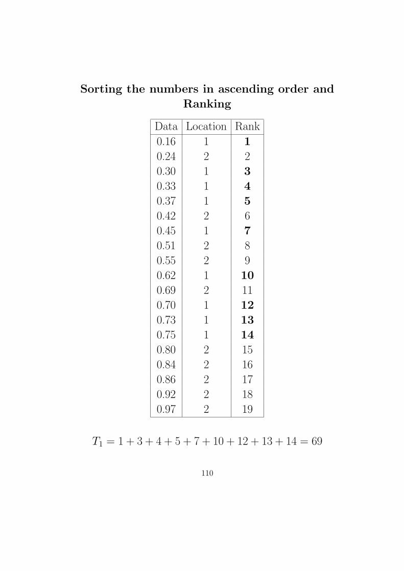
Sorting the numbers in ascending order and
Ranking
Data Location Rank
0.16 1 1
0.24 2 2
0.30 1 3
0.33 1 4
0.37 1 5
0.42 2 6
0.45 1 7
0.51 2 8
0.55 2 9
0.62 1 10
0.69 2 11
0.70 1 12
0.73 1 13
0.75 1 14
0.80 2 15
0.84 2 16
0.86 2 17
0.92 2 18
0.97 2 19
T1 = 1 + 3 + 4 + 5 + 7 + 10 + 12 + 13 + 14 = 69
110
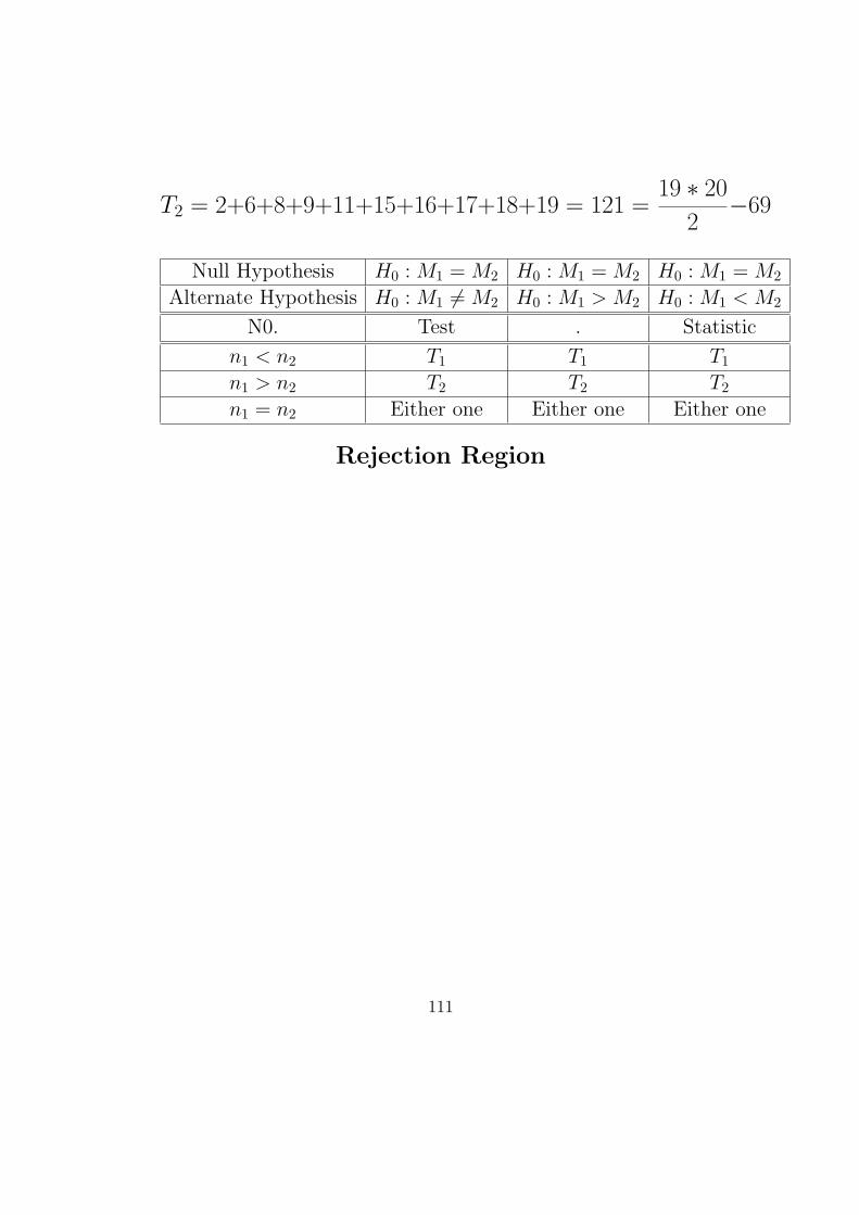
T2 = 2+6+8+9+11+15+16+17+18+19 = 121 =19 ∗ 20
2−69
Null Hypothesis H0 : M1 = M2 H0 : M1 = M2 H0 : M1 = M2
Alternate Hypothesis H0 : M1 6= M2 H0 : M1 > M2 H0 : M1 < M2
N0. Test . Statistic
n1 < n2 T1 T1 T1
n1 > n2 T2 T2 T2
n1 = n2 Either one Either one Either one
Rejection Region
111

Problem:
The following are the burning times of random samples
of two kinds of emergency flares:Brand 1 Brand 2
17.2 13.6
18.1 19.1
19.3 11.8
21.1 14.6
14.4 14.3
13.7 22.5
18.8 12.3
15.2 13.5
20.3 10.9
17.5 14.8
Use the Wilcoxon Rank Sum Test at 0.05 l.o.s to test
whether it is reasonable to say that on the average brand
1 flares are better than Brand 2 flares.
112

Summary of Non Parametric Tests for Final Exam
• ONE SAMPLE SIGN TEST FOR A POPULATIONMEDIAN (Small (n ≤ 30))We are testing , Null Hypothesis H0 : M = 0, M is thepopulation Median.
• WILCOXON SIGNED RANK TEST FOR DEPEN-DENT SAMPLES (Small (n ≤ 30))We are testing , Null Hypothesis H0 : MD = 0, MD is thepopulation Median difference.
• WILCOXON SIGNED RANK TEST FOR DEPEN-DENT SAMPLES (Large (n > 30))We are testing , Null Hypothesis H0 : MD = 0
• COMPARING TWO POPULATION INDEPEN-DENT SAMPLES or WILCOXON RANK SUMTEST (SMALL(n1 ≤ 20 , n2 ≤ 20))We are testing , Null Hypothesis H0 : M1 = M2
M1 and M2 are Population median for sample 1 and sample2 respectively.
• KRUSKAL-WALLIS H-TEST FOR COMPLETELYRANDOMIZED DESIGN (ONE WAY ANOVA)We are testing , Null Hypothesis H0 : M1 = M2 = M3 =... = Mk
113

• FRIEDMAN Fr-TEST FOR COMPLETELY RAN-DOMIZED BLOCK DESIGN (TWO WAY ANOVA)We are testing , Null Hypothesis H0 : Effects of Each Treat-ment = 0, Effect of Each Block = 0
• SPEARMAN’S RANK CORRELATION COEFFI-CIENTWe are testing , Null Hypothesis H0 : ρ = 0, where ρ isthe population correlation between x and y.
114