Embed Size (px)
Citation preview

Roland Meyer
Concurrency Theory
– Lecture Notes –
February 17, 2012
University of Kaiserslautern


Contents
Part I Concurrent Programs and Petri Nets
1 Introduction to Petri Nets . . . . . . . . . . . . . . . . . . . . . . . . . . . . . . . . . . . . . . . 31.1 Syntax and Semantics . . . . . . . . . . . . . . . . . . . . . . . . . . . . . . . . . . . . . . . 31.2 Boundedness . . . . . . . . . . . . . . . . . . . . . . . . . . . . . . . . . . . . . . . . . . . . . . 5
2 Invariants . . . . . . . . . . . . . . . . . . . . . . . . . . . . . . . . . . . . . . . . . . . . . . . . . . . . . 112.1 Marking Equation . . . . . . . . . . . . . . . . . . . . . . . . . . . . . . . . . . . . . . . . . . 112.2 Structural and Transition Invariants . . . . . . . . . . . . . . . . . . . . . . . . . . . . 132.3 Traps and Siphons . . . . . . . . . . . . . . . . . . . . . . . . . . . . . . . . . . . . . . . . . . 152.4 Verification by Linear Programming . . . . . . . . . . . . . . . . . . . . . . . . . . . 17
3 Unfoldings . . . . . . . . . . . . . . . . . . . . . . . . . . . . . . . . . . . . . . . . . . . . . . . . . . . . 233.1 Branching Processes . . . . . . . . . . . . . . . . . . . . . . . . . . . . . . . . . . . . . . . . 243.2 Configurations and Cuts . . . . . . . . . . . . . . . . . . . . . . . . . . . . . . . . . . . . . 263.3 Finite and Complete Prefixes . . . . . . . . . . . . . . . . . . . . . . . . . . . . . . . . . 27
3.3.1 Constructing a finite and complete prefix . . . . . . . . . . . . . . . . 27
4 Coverability . . . . . . . . . . . . . . . . . . . . . . . . . . . . . . . . . . . . . . . . . . . . . . . . . . . 294.1 Coverability Graphs . . . . . . . . . . . . . . . . . . . . . . . . . . . . . . . . . . . . . . . . 29
Part II Network Protocols and Lossy Channel Systems
5 Introduction to Lossy Channel Systems . . . . . . . . . . . . . . . . . . . . . . . . . . . 355.1 Syntax and Semantics . . . . . . . . . . . . . . . . . . . . . . . . . . . . . . . . . . . . . . . 35
6 Well Structured Transition Systems . . . . . . . . . . . . . . . . . . . . . . . . . . . . . . 396.1 Well Quasi Orderings . . . . . . . . . . . . . . . . . . . . . . . . . . . . . . . . . . . . . . . 396.2 Upward and downward closed sets . . . . . . . . . . . . . . . . . . . . . . . . . . . . 416.3 Constructing well quasi orderings . . . . . . . . . . . . . . . . . . . . . . . . . . . . . 426.4 Well Structured Transition Systems . . . . . . . . . . . . . . . . . . . . . . . . . . . 436.5 Abdulla’s Backwards Search . . . . . . . . . . . . . . . . . . . . . . . . . . . . . . . . . 44
v

vi Contents
7 Simple Regularity and Symbolic Forward Analysis . . . . . . . . . . . . . . . . 497.1 Simple Regular Expressions and Languages . . . . . . . . . . . . . . . . . . . . 497.2 Inclusion among simple regular languages . . . . . . . . . . . . . . . . . . . . . . 527.3 Computing the Effect of Transitions . . . . . . . . . . . . . . . . . . . . . . . . . . . 537.4 Computing the Effect of Loops . . . . . . . . . . . . . . . . . . . . . . . . . . . . . . . 547.5 A Symbolic Forward Algorithm for Coverability . . . . . . . . . . . . . . . . 56
8 Undecidability Results for Lossy Channel Systems . . . . . . . . . . . . . . . . . 59
9 Expand, Enlarge, and Check . . . . . . . . . . . . . . . . . . . . . . . . . . . . . . . . . . . . 639.1 Domains of Limits . . . . . . . . . . . . . . . . . . . . . . . . . . . . . . . . . . . . . . . . . 649.2 Underapproximation . . . . . . . . . . . . . . . . . . . . . . . . . . . . . . . . . . . . . . . . 659.3 Overapproximation . . . . . . . . . . . . . . . . . . . . . . . . . . . . . . . . . . . . . . . . . 65
9.3.1 And-Or Graphs . . . . . . . . . . . . . . . . . . . . . . . . . . . . . . . . . . . . . . 669.3.2 Over(TS,Γ ′,L′) . . . . . . . . . . . . . . . . . . . . . . . . . . . . . . . . . . . . . 66
9.4 Overall Algorithm . . . . . . . . . . . . . . . . . . . . . . . . . . . . . . . . . . . . . . . . . . 68
Part III Dynamic Networks and π-Calculus
10 Introduction to π-Calculus . . . . . . . . . . . . . . . . . . . . . . . . . . . . . . . . . . . . . . 7310.1 Syntax . . . . . . . . . . . . . . . . . . . . . . . . . . . . . . . . . . . . . . . . . . . . . . . . . . . . 7410.2 Names and Substitutions . . . . . . . . . . . . . . . . . . . . . . . . . . . . . . . . . . . . 7510.3 Structural Congruence . . . . . . . . . . . . . . . . . . . . . . . . . . . . . . . . . . . . . . 7610.4 Transition Relation . . . . . . . . . . . . . . . . . . . . . . . . . . . . . . . . . . . . . . . . . 77
11 A Petri Net Translation of π-Calculus . . . . . . . . . . . . . . . . . . . . . . . . . . . . 7911.1 Restricted Form . . . . . . . . . . . . . . . . . . . . . . . . . . . . . . . . . . . . . . . . . . . . 8011.2 Structural Semantics . . . . . . . . . . . . . . . . . . . . . . . . . . . . . . . . . . . . . . . . 82
12 Structural Stationarity . . . . . . . . . . . . . . . . . . . . . . . . . . . . . . . . . . . . . . . . . . 8712.1 Structural Stationarity and Finiteness . . . . . . . . . . . . . . . . . . . . . . . . . . 8712.2 Derivatives . . . . . . . . . . . . . . . . . . . . . . . . . . . . . . . . . . . . . . . . . . . . . . . . 8812.3 First Characterization of Structural Stationarity . . . . . . . . . . . . . . . . . . 8912.4 Second Characterization of Structural Stationarity . . . . . . . . . . . . . . . 91
13 Undecidability Results . . . . . . . . . . . . . . . . . . . . . . . . . . . . . . . . . . . . . . . . . . 9513.1 Counter Machines . . . . . . . . . . . . . . . . . . . . . . . . . . . . . . . . . . . . . . . . . . 9513.2 From Counter Machines to Bounded Breadth . . . . . . . . . . . . . . . . . . . 9613.3 Undecidability of Structural Stationarity . . . . . . . . . . . . . . . . . . . . . . . 9813.4 Undecidability of Reachability in Depth 1 . . . . . . . . . . . . . . . . . . . . . . 100

List of Figures
1.1 Tree computation in the decision procedure for boundedness. . . . . . . . 71.2 Petri net N0 computing A0(x) := x+1. . . . . . . . . . . . . . . . . . . . . . . . . . . 91.3 Petri net Nn+1 computing An+1(x+1) := An(An+1(x)). . . . . . . . . . . . . 10
3.1 Unfolding procedure. . . . . . . . . . . . . . . . . . . . . . . . . . . . . . . . . . . . . . . . . 28
4.1 Coverability graph computation. . . . . . . . . . . . . . . . . . . . . . . . . . . . . . . . 31
7.1 Symbolic forward algorithm for coverability in LCS. . . . . . . . . . . . . . . 57
8.1 Sketch of the lossy channel system in the encoding of CPCP . . . . . . . 608.2 Non-computability of channel contents . . . . . . . . . . . . . . . . . . . . . . . . . 62
9.1 Expand, Enlarge, and Check. . . . . . . . . . . . . . . . . . . . . . . . . . . . . . . . . . 69
11.1 Graph interpretation of a π-Calculus process . . . . . . . . . . . . . . . . . . . . . 8011.2 Illustration of unnecessary transitions . . . . . . . . . . . . . . . . . . . . . . . . . . . 8411.3 Structural semantics of an example process . . . . . . . . . . . . . . . . . . . . . . 8511.4 Illustration of the transition system isomorphism in Theorem 11.1 . . . 86
12.1 Transition sequence illustrating unbounded breadth . . . . . . . . . . . . . . . 9112.2 Transition sequence illustrating unbounded depth . . . . . . . . . . . . . . . . . 92
13.1 Proof of undecidability of structural stationarity . . . . . . . . . . . . . . . . . . 98
vii


Part IConcurrent Programs and Petri Nets

Concurrent programs, communicating asynchronously over a shared memory orsynchronously via remote method invocation, can be conveniently modelled interms of Petri nets. We introduce the basics of place/transition Petri nets, discussfundamental verification problems, and study related analysis algorithms.

Chapter 1Introduction to Petri Nets
Abstract First definitions on Petri nets and the notion of boundedness.
1.1 Syntax and Semantics
We present the basic concepts of Petri nets along the lines of [?, ?, ?]. Differentfrom classical textbooks, we put some emphasis verification problems like deadlockfreedom, reachability, coverability, and boundedness.
Definition 1.1 (Petri net). A Petri net is a triple N = (S,T,W ) where S is a finiteset of so-called places, T a finite set of transitions, and W : (S×T )∪ (T ×S)→ Na weight function. Places and transitions are disjoint, S∩T = /0.
Graphically, we represent places by circles, transitions by boxes, and the weightfunction by directed edges. More precisely, for W (s, t) = k with k ∈ N we draw anedge from s to t that is labelled by k, and similar for edges W (t,s) from t to s. Weomit edges weighted zero, and draw unlabelled ones if the weight is one.
The preset •s of a place s ∈ S contains the transitions with an arc leading tothis place, •s := t ∈ T | W (t,s) > 0. Those transitions act productive on s. Thetransitions that consume from s are in the postset of s, s• := t ∈ T | W (s, t)> 0.For transitions t ∈ T , the notions are similar. They operate upon the places in theirpreset •t := s ∈ S | W (s, t)> 0 and in their postset t• := s ∈ S | W (t,s)> 0.
Petri nets are automata comparable to finite state automata or Turing machines.Like every automaton model, they come equipped with a notion of state — called amarking in Petri nets — that influences the actions taken along a computation. Whatdifferentiates Petri nets from the remaining automata is the concurrency they reflect.A single Petri net typically captures the interaction of several programs. Therefore, amarking has to determine the next actions in all programs. The solution is to collectthe places the different programs are currently in.
Definition 1.2 (Marking and marked Petri net). Let N = (S,T,W ). A marking is afunction M ∈NS that assigns a natural number to every place. A marked Petri net is a
3

4 1 Introduction to Petri Nets
pair (N,M0) of a Petri net and an initial marking M0. We also write N =(S,T,W,M0)for a marked Petri net.
Markings are visualised by tokens, dots inserted into the circles that represent theplaces of a Petri net. For M(s) = k with k ∈ N we put k dots into the correspondingcircle and say that place s contains k tokens.
To assess the complexity of verification problems for Petri nets, we measure theirsize by counting the number of places, transitions, arcs, and tokens.
Definition 1.3 (Size of a Petri net). The size of N = (S,T,W,M0) is ||N|| := |S|+|T |+∑s∈S ∑t∈T (W (s, t)+W (t,s))+∑s∈S M0(s).
The execution of transitions, called firing and denoted by1 M1[t〉M2, changes thetoken count. But as markings are defined to be semi-positive, there is a restriction.A transition can only be fired if the places in its preset contain enough tokens.
Definition 1.4 (Enabledness and deadlock). Consider N = (S,T,W ) and M ∈ NS.Transition t ∈ T is enabled in M if M ≥W (−, t). Marking M is a deadlock of N if itdoes not enable any transition.
The detection of deadlocks in a concurrent program is a fundamental problem inverification. Deadlocks point to incorrect assumptions on the synchronisation be-haviour and thus to major flaws in the system of interest.
If transition t is enabled, its firing produces W (t,s) tokens on every place s in itspostset and, at the same time, consumes W (s, t) tokens from the places in its preset.
Definition 1.5 (Firing relation). Let N =(S,T,W ). By definition, the firing relation[〉 ⊆NS×T ×NS contains the triple (M1, t,M2), denoted by M1[t〉M2, if t is enabledin M1 and M2 = M1−W (−, t)+W (t,−).
We extend the firing relation to finite sequences of transitions σ ∈ T ∗ inductivelyas follows. The empty word ε does not change a marking, M[ε〉M for all M ∈ NS.For any two markings M1,M2 ∈NS we then have M1[σ .t〉M2 if there is M ∈NS withM1[σ〉M and M[t〉M2. The syntax M1[σ〉 indicates that transition sequence σ ∈ T ∗
is enabled in M1, which means there is a marking M2 ∈ NS so that M1[σ〉M2. Aninfinite transition sequence σ ∈ T ω is enabled in M1, if so are all its finite prefixes.This means for all σa ∈ T ∗ and σb ∈ T ω with σ = σa.σb we have M1[σa〉.
Definition 1.6 (Termination). A Petri net N =(S,T,W,M0) terminates if no infinitetransition sequence is enabled in M0.
Termination is a second elementary problem in verification. Infinite transition se-quences point to livelocks in a concurrent program, where components fail to leavecertain commands.
A marking M2 is said to be reachable from marking M1, if there is a firing se-quence leading from M1 to M2. We denote the set of all markings reachable fromM1 by R(M1) := M2 ∈ NS | M1[σ〉M2 for some σ ∈ T ∗. For the initial marking,
1 Automata theory commonly uses the syntax M1t→M2 for the execution of transitions.
1.2 Boundedness 5
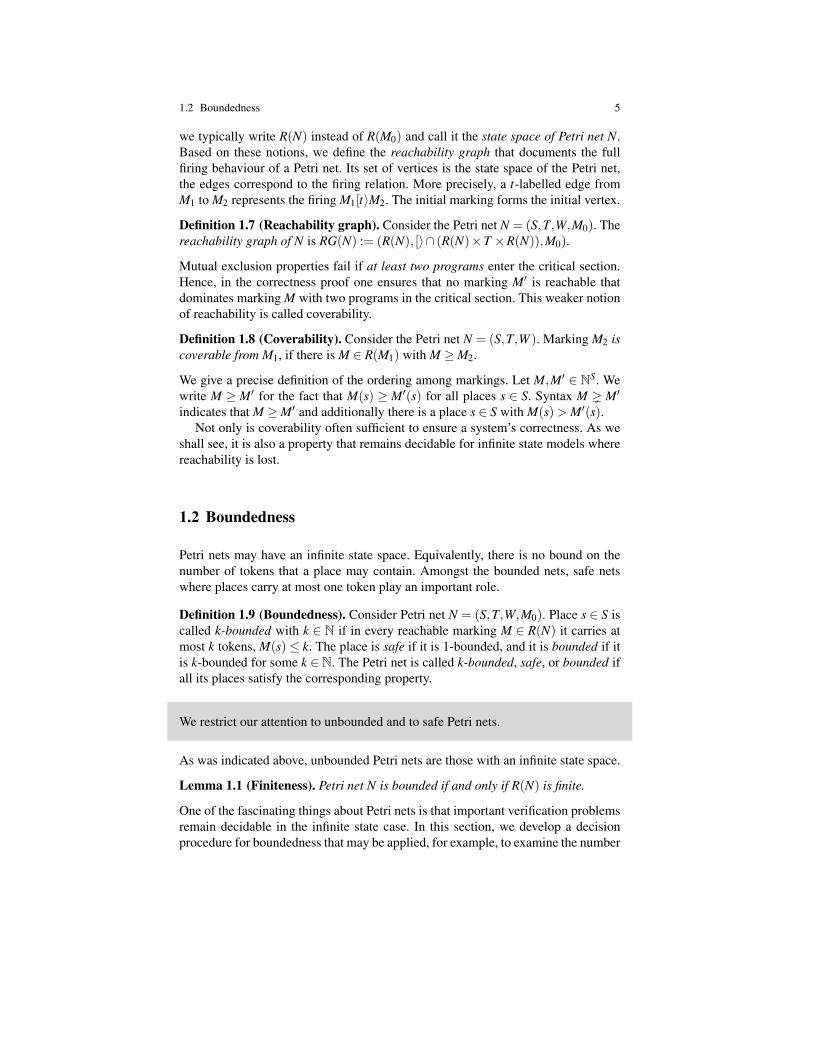
we typically write R(N) instead of R(M0) and call it the state space of Petri net N.Based on these notions, we define the reachability graph that documents the fullfiring behaviour of a Petri net. Its set of vertices is the state space of the Petri net,the edges correspond to the firing relation. More precisely, a t-labelled edge fromM1 to M2 represents the firing M1[t〉M2. The initial marking forms the initial vertex.
Definition 1.7 (Reachability graph). Consider the Petri net N = (S,T,W,M0). Thereachability graph of N is RG(N) := (R(N), [〉∩ (R(N)×T ×R(N)),M0).
Mutual exclusion properties fail if at least two programs enter the critical section.Hence, in the correctness proof one ensures that no marking M′ is reachable thatdominates marking M with two programs in the critical section. This weaker notionof reachability is called coverability.
Definition 1.8 (Coverability). Consider the Petri net N = (S,T,W ). Marking M2 iscoverable from M1, if there is M ∈ R(M1) with M ≥M2.
We give a precise definition of the ordering among markings. Let M,M′ ∈ NS. Wewrite M ≥ M′ for the fact that M(s) ≥ M′(s) for all places s ∈ S. Syntax M M′
indicates that M ≥M′ and additionally there is a place s ∈ S with M(s)> M′(s).Not only is coverability often sufficient to ensure a system’s correctness. As we
shall see, it is also a property that remains decidable for infinite state models wherereachability is lost.
1.2 Boundedness
Petri nets may have an infinite state space. Equivalently, there is no bound on thenumber of tokens that a place may contain. Amongst the bounded nets, safe netswhere places carry at most one token play an important role.
Definition 1.9 (Boundedness). Consider Petri net N = (S,T,W,M0). Place s ∈ S iscalled k-bounded with k ∈ N if in every reachable marking M ∈ R(N) it carries atmost k tokens, M(s)≤ k. The place is safe if it is 1-bounded, and it is bounded if itis k-bounded for some k ∈ N. The Petri net is called k-bounded, safe, or bounded ifall its places satisfy the corresponding property.
We restrict our attention to unbounded and to safe Petri nets.
As was indicated above, unbounded Petri nets are those with an infinite state space.
Lemma 1.1 (Finiteness). Petri net N is bounded if and only if R(N) is finite.
One of the fascinating things about Petri nets is that important verification problemsremain decidable in the infinite state case. In this section, we develop a decisionprocedure for boundedness that may be applied, for example, to examine the number

6 1 Introduction to Petri Nets
of threads a server may generate. The argumentation serves as an appetiser for theproofs that are about to follow in this lecture. In particular, the idea of monotonicityappears in different flavours. Technically, monotonicity states that larger markingsare able to imitate the behaviour of smaller ones.
Lemma 1.2 (Monotonicity). Consider a Petri net N = (S,T,W ) and markingsM,M1,M2 ∈ NS. If M1[σ〉M2 then (M1 +M)[σ〉(M2 +M).
Monotonicity shows that sequences of increasing markings point to an infinite statespace.
Lemma 1.3 (From increasing markings to unboundedness). Consider some Petrinet N. If there are M1 ∈ R(N) and M2 ∈ R(M1) with M2 M1, then N is unbounded.
Idea. By monotonicity, a transition sequence σ from M1 to M2 with M2 M1 can berepeated in M2. It leads to a marking M3 with M3 M2 for which the argumentationagain holds. We thus obtain
M0[τ〉M1[σ〉M2[σ〉M3[σ〉 . . . with M1 M2 M3 . . .
The sequence adds an unbounded number of tokens to at least one place.
Proof. Assume M0[τ〉M1[σ〉M2 with M2 M1 and σ ,τ ∈ T ∗. Since M2 M1, thedifference M := M2−M1 is greater zero, M 0. The observation that M2 = M1+Mnow justifies M1[σ〉(M1 +M). With monotonicity in Lemma 1.2, we add M to M1and have (M1 + M)[σ〉(M1 + 2M). This means, sequence σ can also be fired inM1 +M. Repeating the argumentation shows that M1[σ
i〉(M1 + iM) for every i ∈N.To establish unboundedness, we proceed by contradiction. Let k ∈ N bound
the token count in all markings on all places. Since M 0, there is a places ∈ S with M(s) > 0. We argued above that firing σ for (k + 1)-times is feasi-ble and yields M1[σ
k+1〉(M1 +(k+ 1)M). In the resulting marking, place s carries(M1 +(k+ 1)M)(s) = M1(s)+ (k+ 1)M(s) ≥ k+ 1 tokens, which contradicts theboundedness assumption. ut
Interestingly, also the reverse holds. If a Petri net is unbounded, one finds the tokencount increasing on some path. The proof relies on the fact that NS is well-quasi-ordered. Every infinite sequence of markings (Mi)i∈N contains comparable elementsi < j with Mi ≤M j. We devote the full Section ?? to well-quasi-orderings and takethis fact for granted.
Lemma 1.4 (Comparable elements). Consider Petri net N. Every infinite sequence(Mi)i∈N of markings in R(N) contains indices i < j with Mi ≤M j.
Lemma 1.5 (From unboundedness to increasing markings). If N is unbounded,then there are M1 ∈ R(N) and M2 ∈ R(M1) with M2 M1.
Idea. We summarise all transition sequences that do not repeat markings in a tree.To be precise, we say that a transition sequence M0[t1〉M1[t2〉 . . . [tn〉Mn does notrepeat markings, if Mi 6= M j for all i 6= j. Note that every reachable marking can

1.2 Boundedness 7
be obtained without repetitions. Hence, as we have an infinite state space, the treeis infinite. The outdegree is bounded by the number of transitions. An applicationof Konig’s lemma2 now shows the existence of an infinite path (Mi)i∈N in this tree.Lemma 1.4 gives two comparable elements i < j with Mi ≤ M j on the path. Byconstruction, the markings are distinct, Mi M j, as required.
Proof. Consider the unbounded Petri net N = (S,T,W,M0). We construct a tree(Q,→,q0, lab) with vertices Q, edges→⊆Q×T ×Q, root q0, and vertex labellinglab that assigns to every q ∈ Q a marking M ∈ NS. The procedure, stated in pseudocode in Figure 1.1, works as follows. The root q0 is labelled by the initial marking.For every vertex q1 ∈Q labelled by M1 and every transition t ∈ T , compute M2 withM1[t〉M2. If M2 does not label a vertex on the path from q0 to q1, add a new vertexq2 to the tree and label it by M2. Add the edge (q1, t,q2). If transition t is disabledin M1 or M2 has already been seen, consider the next transition.
lab(q0) = M0
for all q1 ∈ Q dofor all t ∈ T do
let lab(q1) = M1
if M1[t〉M2 and M2 does not label a vertex on the path from q0 to q1 thenadd new vertex q2 to Q with lab(q2) = M2
add edge (q1, t,q2) to→(♠) //decision procedure in Theorem 1.1
end ifend for all
end for all(♣) //decision procedure in Theorem 1.1
Fig. 1.1 Tree computation in the decision procedure for boundedness.
Since N is unbounded, its state space is infinite according to Lemma 1.1. Everymarking M ∈ R(N) is reachable without repetitions and thus labels some q ∈ Q.Therefore, the tree computed above is infinite. Its outdegree is bounded by thenumber of transitions, hence finite. By Konig’s lemma, there is an infinite pathq0, t1,q1, t2,q2, t3 . . . in the tree with (qi, ti+1,qi+1) ∈ → for all i ∈ N. Its vertexlabelling lab(qi) = Mi forms an infinite sequence of markings (Mi)i∈N for whichLemma 1.4 finds two comparable elements Mi≤M j with i< j. They are different byconstruction, Mi M j. The observation that edges represent transition firings yieldsM0[t1〉M1[t2〉M2[t3〉 . . . and allows us to conclude Mi ∈ R(M0) and M j ∈ R(Mi). ut
The proof of Lemma 1.5 suggests the following decision procedure for bounded-ness. Compute the tree of all transition sequences and report unboundedness at (♠)
2 Konig’s lemma states that every infinite tree of finite outdegree contains an infinite path.

8 1 Introduction to Petri Nets
when increasing markings are found. If no such markings exist, the computationeventually stops and returns boundedness at (♣). The procedure is correct for both,depth-first and breadth-first implementations of the tree computation.
Theorem 1.1 (Decidability of boundedness). It is decidable, whether a Petri net Nis bounded.
To turn the algorithm given in Figure 1.1 into a decision procedure for boundedness,add the following commands at the points specified:
(♠) if M2 M for some M labelling a vertex on the path from q0 to q1 thenreturn unbounded
end if
(♣) return bounded
Proof. To establish correctness, assume the decision procedure is applied to anunbounded Petri net. By Lemma 1.5, there are M1 ∈ R(N) and M2 ∈ R(M1) withM2 M1. Hence, a breadth-first implementation of the tree computation will findvertices q1 reachable from q0 and labelled by M1 as well as q2 reachable from q1and labelled by M2. The if condition in (♠) applies and returns unbounded.
The proof of Lemma 1.5 actually shows that every infinite path contains twocomparable elements M2 M1. Hence, a depth-first implementation either finds(♠) satisfied or backtracks from a finite path. As the tree contains an infinite path,the search eventually returns the correct answer.
If the algorithm is applied to a bounded Petri net, by Lemma 1.3 (contraposition)there are no M1 ∈R(N) and M2 ∈R(M1) with M2 M1. Condition (♠) never applies.However, as the Petri net is bounded its state space is finite by Lemma 1.1. The treecomputation eventually stops and returns bounded at (♣). ut
For bounded Petri nets, the decision procedure determines the full state space. Todemonstrate that this leads to unacceptable runtimes, we present a construction byErnst Mayr (∗1950) and Albert Meyer (∗1941). It provides bounded Petri nets of sizeO(n) that generate the astronomic number of A(n) tokens. The Ackermann functionA(n) is well known to be not primitive recursive.
Definition 1.10 (Ackermann function). Consider the functions Ai ∈NN defined by
A0(x) := x+1 An+1(0) := An(1) An+1(x+1) := An(An+1(x))
The Ackermann function A ∈ NN is defined as A(n) := An(n).
Theorem 1.2 (Mayr and Meyer [?]). For every n ∈N, there is a bounded Petri netNn of size O(n) that generates A(n) tokens on some place.
As a consequence, there is no primitive recursive relationship between the size of abounded Petri net and the size of its state space.

1.2 Boundedness 9
Corollary 1.1. For bounded Petri nets N, the size of R(N) and thus RG(N) is notbounded by a primitive recursive function in the size of N.
Proof (of Theorem 1.2). We follow the presentation in [?]. The sequence of Petrinets Nn is constructed inductively. To this end, we equip them with four interfaceplaces. A starting and a halting place control the computation so that the Petri netsterminate when the halting place gets marked. The input place expects x ∈N tokensand the transition sequences produce up to An(x) tokens on the output place.
Let Nn(x) mean that the input of Nn contains x ∈N tokens and the start place hasa single token. The remaining places are unmarked. To make our statement precise,we require that Nn(x) is bounded by An(x). The Petri net terminates. Moreover,M ∈ R(Nn(x)) is a deadlock if and only if M(stop) = 1 and M(start) = 0. There issuch a deadlock with M(stop) = 1, M(out) = An(x), and M(s) = 0 otherwise.
Petri net N0 is depicted in Figure 1.2. It moves all tokens on the input placeto the output place, and finally adds one token before halting. The conditions onboundedness and termination are readily checked.
Fig. 1.2 Petri net N0 comput-ing A0(x) := x+1.
start
in
stop
out
Petri net Nn+1 extends Nn by connecting to the interface places. The construction,given in Figure 1.3, exploits the equation
An+1(x) = An(. . .An(An︸ ︷︷ ︸(x+1)−times
(1)) . . .).
To compute An+1(x) with Nn+1(x), observe that by the induction hypothesis Nn(1)always terminates with a token on stop. Among the transition sequences there is onethat, upon halting, gives An(1) tokens on the output place and an otherwise (up tostop) empty net Nn. We transfer the tokens back to the input place of Nn, therebydecrementing x. This restarts Nn with input An(1), Nn(An(1)). We again apply thehypothesis to find a terminating run that produces An(An(1)) tokens on the outputplace of Nn. This means, we have An+1(1) tokens on the output place of Nn and stillx− 1 tokens in the input place of Nn+1. Repeating the computation and transfer ofNn for another (x−1)-times provides An+1(x) tokens on the output place of Nn. ThePetri net cannot be restarted as no tokens are left on the input of Nn+1. Instead theAn+1(x) tokens on the output of Nn are transferred to the output of Nn+1. Petri netNn+1(x) then halts with the required token count. In Figure 1.3, the start of Nn on 1as well as the loop construction from the output place of Nn back to its input placeare highlighted in red and blue, respectively.
Petri net Nn+1(x) does not guarantee that all tokens on the output place of Nnare transferred back to the input. This does not lead to a bound larger than An+1(x).Assume we transfer y tokens and x tokens remain in the output place of Nn. After

10 1 Introduction to Petri Nets
start
in
strt
inNn
stp
out
stop
out
Fig. 1.3 Petri net Nn+1 computing An+1(x+1) := An(An+1(x)).
the computation of Nn(y), we find at best An(y)+ x tokens on the output of Nn. ByAn(y)+x≤ An(y+x), keeping tokens in the output place only decreases the overalltoken count. Hence, An+1(x) in fact bounds the token count of Nn+1(x).
The size of N0 is 17. For Nn, we add 33 items to the size of Nn−1 and obtain
||Nn||= 33+ ||Nn−1||= 33n+17.
Initially, the input place of Nn carries n tokens and the start place has a single token.The marked Petri net thus has a size of 34n+18 ∈ O(n). ut

Chapter 2Invariants
Abstract Linear programming techniques for Petri net verification.
2.1 Marking Equation
Our goal is to exploit linear algebraic techniques for reasoning about (un)reachabilityand (non)coverability of markings. To this end, we rephrase the firing relation as alinear algebraic operation. As a first step, equip the set of places in N = (S,T,W,M0)with a total ordering that we indicate by indices S = s1, . . . ,sn. It turns markingM ∈ NS into a vector M ∈ N|S| of dimension |S|. Similarly, for a fixed transitiont ∈ T the weight function W : (S×T )∪(T ×S)→N is expressed by the two vectors
W (−, t) :=
W (s1, t)...
W (sn, t)
W (t,−) :=
W (t,s1)...
W (t,sn)
in N|S|.
With an additional ordering on transitions, T = t1, . . . , tm, the weight function Wyields two matrices. The forward matrix F ∈ N|S|×|T | contains the weights on arcsfrom places to transitions, i.e., forward relative to the places. The backwards matrixB ∈ N|S|×|T | gives the arcs from transitions to places:
F :=(
W (−, t1) . . . W (−, tm))
B :=(
W (t1,−) . . . W (tm,−)).
Together, forward and backward matrix contain full information about the weightfunction so that we may alternatively give N = (S,T,W ) as N = (S,T,F,B).
Definition 2.1 (Connectivity matrix). Let N = (S,T,F,B). Its connectivity matrixis C := B−F ∈ Z|S|×|T |.
11

12 2 Invariants
The connectivity matrix does not indicate loops in the Petri net. If there are arcsfrom place s to transition t and vice versa, W (s, t) = 1 =W (t,s), we get C(s, t) = 0.Missing arcs with W (s, t) = 0 =W (t,s) have the same entry.
The i-th column of C gives the difference W (ti,−)−W (−, ti), which is preciselythe vector added to a marking upon firing of ti. With this insight, we can determinethe goal marking M2 reached from M1 via a full transition sequence σ directly fromM1 and σ , without intermediary firings. The key is that just the number of transitionsbut not their ordering in a firing sequence is important.
Definition 2.2 (Parikh image). Consider transitions T . The Parikh image of σ ∈ T ∗
is the function p(σ) ∈ NT with (p(σ))(t) = number of occurrences of t in σ .
To illustrate the independence of the transition ordering, consider some sequenceσ = t1.t2.t1 over two transitions. If M1[σ〉M2 by definition of firing M2 satisfies
M2 = M1 +C(−, t1)+C(−, t2)+C(−, t1)= M1 +C(−, t1)(p(σ)(t1))+C(−, t2)(p(σ)(t2)).
Taking the Parikh image as a vector, this sum is M0 +C · p(σ).
Lemma 2.1 (Marking equation). Consider N = (S,T,W ) with connectivity matrixC ∈ N|S|×|T |, M1,M2 ∈ N|S|, and σ ∈ T ∗. If M1[σ〉M2 then M2 = M1 +C · p(σ).
As an immediate consequence, if marking M2 is reachable from M1 the equationM2−M1 = C · x has a solution in N|T |. This can be applied in contraposition forverification. If the equation has no solution then M2 is not reachable from M1.
Vice versa, any vector K ∈ N|T | is the Parikh image of a transition sequence,K = p(σ) for some σ ∈ T ∗. This σ has an enabling marking, say M1 ∈N|S|. Hence,the following weak reverse of the above holds. If M = C · x has a natural solution,then there is a marking M1 that reaches M1 +M. We summarise both arguments.
Lemma 2.2. Consider N = (S,T,F,B) with connectivity matrix C∈N|S|×|T | and letM ∈N|S|. There is a marking M1 ∈N|S| with M1+M ∈ R(M1) if and only if M =C ·xhas a solution in N|T |.
Interestingly, in combination with the statements on boundedness from Section 1.2,Lemma 2.2 provides a characterisation of structural boundedness, i.e., boundednessunder any initial marking.
Proposition 2.1 (Characterisation of structural boundedness). Consider Petrinet N =(S,T,F,B) with connectivity matrixC∈N|S|×|T |. There is an initial markingM0 so that (N,M0) is unbounded if and only if C · x 0 has a solution in N|T |.
Proof. For the direction from right to left, assume C · x 0 has a solution in N|T |.This means, there is a marking M 0 with C · x = M. By Lemma 2.2, we find amarking M1 with M1 +M ∈ R(M1). We are thus in a position to apply Lemma 1.3to the Petri net N with initial marking M1, which proves unboundedness. ut

2.2 Structural and Transition Invariants 13
Parametric verification considers families of systems where the instances differ onlyin certain parameters. A typical example are client server architectures that vary inthe number of threads. In this light, Proposition 2.1 can be interpreted as follows.Solving C · x 0 checks for whether the size, for example of buffers, is bounded inall instances of the architectural family.
2.2 Structural and Transition Invariants
In our running example, we noticed that always either the semaphore or the criticalsection carries a token. This can be formulated as
M(pcs)+M(sem) = 1, (2.1)
and the equation holds in every reachable marking. Structural invariants provide ameans to derive such equations. Technically, a structural invariant is a vector I ∈Z|S|with CT · I = 0. Here, CT denotes the transpose of the connectivity matrix, andtherefore I is in fact an |S|-dimensional vector. The intuition is that I gives a weightto the tokens on each place.
Definition 2.3 (Structural invariant). Consider N = (S,T,W ) with connectivitymatrix C ∈ Z|S|×|T |. A structural invariant I ∈ Z|S| is a solution to CT · x = 0.
The main property of structural invariants is that the I-weighted sum of tokens staysconstant under transition firings. This follows, by a beautiful algebraic trick, fromthe marking equation and the requirement that CT · I = 0.
Theorem 2.1 (Invariance of structural invariants). Let I ∈ Z|S| be a structuralinvariant of N = (S,T,W,M0). Then for all M ∈ R(N) we have IT ·M = IT ·M0.
Before we turn to the proof, we show how to derive Equation 2.1 in our examplewith the help of Theorem 2.1. Note that I(pw) = 0 and I(pcs) = 1 = I(sem) is astructural invariant of NM+S. The initial marking is M0(pw) = 2, M0(sem) = 1, andM0(pcs) = 0. An application of Theorem 2.1 yields
IT ·M = 0M(pw)+1M(pcs)+1M(sem) = 1 = IT M0,
as required. The equation holds for all markings reachable in NM+S.
Idea (Theorem 2.1). The proof relies on the marking equation M = M0 +C · p(σ).We multiply the invariant from the left and exploit the laws of transposition
IT · (C · p(σ)) = (CT · I)T · p(σ)
to swap the positions of I and C. The definition of structural invariants concludesthe proof.

14 2 Invariants
Proof. Let N = (S,T,W,M0) be a Petri net with connectivity matrixC∈Z|S|×|T | andstructural invariant I ∈ Z|S|. Assume marking M ∈ R(N) is reachable by M0[σ〉Mfor some σ ∈ T ∗. The marking equation yields M = M0 +C · p(σ). We multiply thetransposed of I to both sides and obtain
IT ·MMarking equation = IT · (M0 +C · p(σ))
Distributivity = IT ·M0 + IT · (C · p(σ))
Associativity, transposition self inverse = IT ·M0 +(IT ·CT T) · p(σ)
Transposition law BT ·AT = (A ·B)T = IT ·M0 +(CT · I)T · p(σ)
Definition structural invariant = IT ·M0 +0T · p(σ).
The latter is IT ·M0 which concludes the proof. utApplied in contraposition, Theorem 2.1 yields a reachability check. If a markingdoes not satisfy the equality stated above, it cannot be reachable.
Corollary 2.1 (Unreachability via structural invariants). Let N = (S,T,W,M0)with structural invariant I ∈ Z|S| and M ∈ N|S|. If IT ·M 6= IT ·M0, then M /∈ R(N).
Structural invariants can be computed in polynomial time using Gauss eliminationwith O(||N||3). Therefore, this test can be performed efficiently prior to heavierreachability analyses. To obtain more expressive structural invariants, they can beadded up and scaled by a constant.
Lemma 2.3. If I1 and I2 are structural invariants of N, so are I1 + I2 and kI1, k ∈ Z.
Invariants also yield bounds for the places that are weighted strictly positive. Thelemma follows from Theorem 2.1 and only holds for non-negative invariants.
Lemma 2.4 (Place boundedness from structural invariants). Let N = (S,T,W )with structural invariant I ∈ N|S|. Let s ∈ S with I(s) > 0. Then s is bounded underany initial marking M0 ∈ N|S|.As a consequence, a Petri net N = (S,T,W ) that has a covering structural invariantI ∈ N|S| with I(s)> 0 for all s ∈ S is bounded under any initial marking.
Corollary 2.2 (Structural boundedness from structural invariants). If N has acovering structural invariant, it is structurally bounded.
Definition 2.4 (Transition invariant). Consider N = (S,T,W ) with connectivitymatrix C ∈ Z|S|×|T |. A transition invariant J ∈ N|T | is a solution to C · x = 0.
Transition sequences with Parikh vector J do not change the marking. Vice versa,if a transition sequence does not change the marking, then its Parikh vector is atransition invariant.
Theorem 2.2 (Invariance of transition invariants). Consider transition sequenceM[σ〉M′ in a Petri net N = (S,T,W ). Then M′ =M if and only if p(σ) is a transitioninvariant of N.
Transition invariants again can be added up and scaled by a constant. Reachabilitygraphs of Petri nets without transition invariants are acyclic.

2.3 Traps and Siphons 15
2.3 Traps and Siphons
Petri nets are bipartite graphs. Up to now, we have used this fact only indirectlywhen we defined the connectivity matrix. In this section, we explictily use the graphstructure to derive inequalities on the token count that are invariant under firings.The corresponding notions of siphons and traps are classical in Petri net theory.They describe regions of places in a Petri net that tokens can never leave or enter.
Traps and siphons can be defined for Petri nets with weighted arcs, but this causesa formal overhead. We therefore assume that transitions are weighted either zero orone. More formally, in this section we consider ordinary Petri nets N = (S,T,W )where W : (S×T )∪ (T ×S)→0,1.
Definition 2.5 (Trap). A trap is a subset Q ⊆ S of places that satisfies Q• ⊆ •Q. Atrap is said to be marked under M ∈ N|S| if M(q)≥ 1 for some q ∈ Q.
Intuitively, whenever a transition intends to remove tokens from a place in the trap,then the transition will also produce tokens in some place in the trap. The placesneed not coincide. As a consequence, initially marked traps remain marked in allreachable markings.
Lemma 2.5 (Trap property). Let Q be a trap of Petri net N = (S,T,W,M0) that ismarked under M0. Then ∑q∈Q M(q) ≥ 1 holds for all M ∈ R(N).
The inequality may be satisfied by sets of places that do not form a trap. Therefore,the reverse of the implication does not hold. The statement may be interpreted as anecessary condition for reachability.
Corollary 2.3. Let Q⊆ S be an initially marked trap of N and M ∈ N|S| a marking.If ∑q∈Q M(q) = 0 then M is not reachable, M /∈ R(N).
It can be shown that the union of traps again forms a trap. As a consequence, wecan restrict ourselves to families of traps that generate the remaining traps by union.On the one hand, this reduces the effort when computing traps. On the other hand,smaller traps yield more precise inequalities in Lemma 2.5.
Definition 2.6 (Generating family of traps). Let Q1, . . . ,Qn be a family of trapsin a Petri net N. The family is said to be generating if every trap Q of N can beobtained as union of traps in the family, Q=
⋃j∈J Q j for some subset J⊆1, . . . ,n.
A trap is called minimal if it does not contain further traps.
A generating family certainly contains all minimal traps in a Petri net. But in turn,the minimal traps do not necessarily form a generating family. Moreover, there arePetri nets with a single family of generating traps that is exponential in the size of thenet. Therefore, to use traps in verification, we should represent them symbolicallyin some formalism instead of computing them explicitly.
As symbolic formalism, we again target linear programming. We set up a systemof linear inequalities

16 2 Invariants
Y T ·CQ ≥ 0 (2.2)Y ≥ 0
whose rational solutions characterize traps. For the technical development, we firstintroduce a variable Y (s) for every place s ∈ S. By definition, traps Q ⊆ S satisfyQ• ⊆ •Q. For every place s1 ∈ Q and every transition t ∈ s•1 some place s2 ∈ t•
belongs to Q. With place variables, we formulate the requirement equivalently as
Y (s1) ≤ ∑s2∈t•
Y (s2).
Fix s1 ∈ S and t ∈ s•1. To rephrase the above inequality with matrix multiplication, letEs1 denote the unit vector for dimension s1. Moreover, we set up the postset vectorVt• ∈ 0,1|S| with Vt•(s) = 1 iff s ∈ t•. The inequality is then equivalent to
ETs1·Y ≤ V T
t• ·Y ⇔ Y T · (Vt• −Es1) ≥ 0.
To check the inclusion Q•⊆ •Q on all places in a trap and all surrounding transitions,we summarize the above vectors Vt• −Es1 in a matrix.
Definition 2.7 (Trap matrix). The trap matrix CQ ∈ Z|S|×|S||T | is defined by settingCQ(−,(s, t)) :=Vt• −Es if t ∈ s• and CQ(−,(s, t)) := 0 otherwise.
In combination with the equivalences derived above, we obtain a linear algebraiccharacterization of traps. For a concise statement, consider Q ⊆ S. The associatedvector is KQ ∈Q|S| with KQ(s) := 1 if s ∈ Q and KQ(s) := 0 otherwise. Vice versa,every vector K ∈Q|S| describes the set QK := s ∈ S | K(s)> 0.
Proposition 2.2. Consider Petri net N. If Q ⊆ S is a trap, then KQ ∈ Q|S| satisfiesInequality 2.2. In turn, if K ∈Q|S| satisfies Inequality 2.2, then QK ⊆ S is a trap.
The concept dual to traps are so-called siphons. They describe regions in a Petri netthat cannot receive tokens. Technically, every transition that acts productive on theplaces in a siphon also consumes tokens from the siphon.
Definition 2.8 (Siphon). A siphon of Petri net N is a subset D ⊆ S of places thatsatisfies •D⊆ D•. A siphon is empty under M ∈ N|S| if M(s) = 0 for all s ∈ D.
A siphon that is initially empty blocks all transitions that produce tokens on it.
Lemma 2.6 (Siphon property). Consider Petri net N = (S,T,W,M0) with siphonD⊆ S that is empty under the initial marking M0 ∈ N|S|. Then ∑s∈D M(s) = 0 holdsfor all M ∈ R(N).
Like for traps, a union of siphons again yields a siphon. Moreover, empty siphonscharacterize deadlock situations in a Petri net. The statement only holds for Petrinets where every transition depends on a place, i.e., in the following we assume thatfor each t ∈ T there is s ∈ S with s ∈ •t.
Lemma 2.7 (Deadlocks and empty siphons). If M ∈ N|S| is a deadlock of N thenthere is a siphon D⊆ S that is empty under M.

2.4 Verification by Linear Programming 17
Set D := s ∈ S | M(s) = 0 to contain the places that are empty in M. Considert ∈ •D. Since t is dead, there is s ∈ •t with M(s) = 0. This means t ∈ D•.
2.4 Verification by Linear Programming
We develop a powerful constraint-based verification algorithm for Petri nets thatis based on the linear algebraic insights obtained so far. Instead of constructingthe Petri net’s state space, the algorithm sets up a system of inequalities whoseinfeasibility proves correctness. As a consequence, the approach circumvents thestate space explosion problem and is rather fast. Moreover, it is not restricted tofinite state systems. On the downside, the algorithm is only sound but not complete.If it finds the constraint system infeasible, it concludes correctness of the Petri net. Inturn, although the Petri net is correct the algorithm may find the constraint systemfeasible. In this case it returns unknown. To begin with, we make the notion ofcorrectness precise.
Definition 2.9 (Property). A property is a function P : N|S| −→ B that assigns aBoolean value to each marking. We write P(M) rather than P(M)= t and similarly¬P(M) for P(M) = f . A property holds for a Petri net N if P(M) holds forall M ∈ R(N). A property is co-linear if its violation can be expressed by a linearinequality: ¬P(M) if and only if A ·M ≥ B for some A ∈ Qk×|S| and B ∈ Qk forsome k ∈ N.
Definition 2.10 (Linear, integer, mixed programming). A linear programmingproblem is a set of linear inequalities A ·X ≤ B with A ∈ Qm×n and B ∈ Qm on aset of variables X ∈ Qn. The inequalities are also called constraints. There may bean additional objective function CT ·X with C ∈ Qn to be maximized. We denote alinear programming problem by
Variables: X (potentially with type)Maximize CT ·X subject to
A ·X ≤ B.
A solution to the problem is a vector K ∈Qn that satisfies A ·X ≤ B. The solution isoptimal if it maximizes CT ·X in the space of all solutions.
If the solution is required to be integer, K ∈Zn, then the problem is called integerprogramming problem. If some variables are to receive integer values while otherscan be evaluated rational, we have a mixed programming problem. A linear, integer,or mixed programming problem is called feasible if it has a solution. Otherwise it iscalled infeasible.
Linear programming is in P while mixed and integer programming are NP-complete.We explain how integer programming helps checking whether a Petri net N satisfiesa property P . Assume this is not the case. Then there is a marking M ∈ R(N) that

18 2 Invariants
violates the property. Recall that the marking equation overapproximates the statespace. This means M satisfies M = M0 +C ·X for some X ∈ N|T |. By co-linearity,violation ¬P(M) is expressed by A ·M ≥ B. To sum up, a reachable marking thatviolates the property solves the following integer programming problem.
Definition 2.11 (Basic verification system). Consider Petri net N = (S,T,W,M0)and a co-linear property P defined by A ·X ≥ B for some A ∈ Qk×|S| and B ∈ Qk
with k ∈ N. The basic verification system (BVS) associated to N and P is
Variables: X ,M integerM = M0 +C ·X
M,X ≥ 0A ·M ≥ B.
We argued that feasibility of BVS is necessary for a violation to the property.
Proposition 2.3. Consider a Petri net N and a property P . If the associated BVS isinfeasible, then P holds for N.
Basic verification systems are too weak for the analysis of concurrent programs thatcommunicate via shared variables. Programs typically rely on tests of the form
c0; if x = 0 then c1; . . . else . . .
to determine the flow of control. These tests are canonically modelled by loopsin Petri nets. There is a transition t leading from a place for command c0 to aplace for command c1. This transition has arcs from and to a place s that reflectsthe valuation x = 0. In consequence, the connectivity matrix has entry C(s, t) =W (t,s)−W (s, t) = 0. Therefore, the connectivity matrix cannot distinguish the testfrom the absence of a test. As a result, Proposition 2.3 often is not applicable and aproof for unreachability of c1 fails. Indeed, the BVS does not change for programc0;c1 where the latter command is reachable.
To strengthen the verification approach, we refine the set of constraints in BVS.We add inequalities that reflect the trap property: all initially marked traps have toremain marked in the marking that solves the mixed programming problem. Theresulting enhanced verification system is sensitive to guards.
To incorporate traps, we construct for a given marking M a trap inequality. Ithas a rational solution if and only if M satisfies the trap property. Note that it isnot obvious how to check a universal quantifier (all initially marked traps remainmarked in M) by means of feasibility (there is a solution to the trap inequality). Theidea is to state the reverse. We set up a constraint system that is feasible iff there is atrap for which M violates the trap property. Then we use Farkas’ lemma to captureby means of feasibility the negation of this statement: for all traps M satisfies thetrap property. We briefly explain the steps in our construction.
1. We exploit the linear algebraic characterization of traps to set up a system ofinequalities. This so-called primal system is feasible if and only if M violates thetrap property for some trap.

2.4 Verification by Linear Programming 19
2. By Farkas’ lemma we then construct a dual system of inequalities that is feasibleif and only if the primal system is infeasible. Together with the first statement,the dual system is thus feasible if and only if M satisfies the trap property for alltraps.
3. In combination with the marking equation, M becomes variable which leads tonon-linearity of the resulting constraints. We manipulate the constraint system todeal with this.
The primal system is a reformulation of the trap property.
Definition 2.12 (Primal system). Consider Petri net N = (S,T,W,M0) with trapmatrix CQ ∈ Z|S|×|S||T |. Let M ∈ N|S| be some marking. The primal system is
Variables: Y rational
Y T ·CQ ≥ 0Y ≥ 0
Y T ·M0 > 0Y T ·M = 0.
By the first two inequalities, Y forms a trap. The strict inequality then requires Y tobe initially marked, and the equality finds Y unmarked at M. As a result, M violatesthe trap property for QY from Proposition 2.2.
Lemma 2.8. The primal system is feasible if and only if M violates the trap property.
For the second phase of our construction, we briefly recall Farkas’ lemma. Certainsystems of inequalities, so-called primal systems, have a dual system that enjoys thefollowing equivalence. The primal system is infeasible if and only if the dual systemis feasible.
Lemma 2.9 (Farkas 1894). One and only one of the following linear programmingproblems is feasible:
Variables: X rational Variables: Y rational
A ·X ≤ B Y T ·A≥ 0X ≥ 0 Y T ·B < 0
Y ≥ 0.
The system from Definition 2.12 is not quite in the form on the right hand side.We apply several transformations to obtain an equivalent constraint system of therequired shape. Equivalent here means that the solutions do not change. To beginwith, note that M ∈ N|S| and thus M ≥ 0. Moreover, we require Y ≥ 0. Hence, wehave Y T ·M = 0 if and only if Y T ·M ≤ 0. Changing the signs inverts the inequality,i.e., Y T ·M≤ 0 holds if and only if Y T ·(−M)≥ 0. We treat M0 similarly and rewritethe system from Definition 2.12 to

20 2 Invariants
Variables: Y rational
Y T ·CQ ≥ 0Y ≥ 0
Y T · (−M0)< 0Y T · (−M)≥ 0.
A last step in constructing the desired shape is to extend CQ by a column for −M,denoted by (CQ −M). This summarize the first and the last inequality. Indeed, wehave Y T ·CQ ≥ 0 and Y T · (−M)≥ 0 if and only if Y T · (CQ −M)≥ 0.
Variables: Y rational
Y T · (CQ −M)≥ 0Y T · (−M0)< 0
Y ≥ 0.
To this system, we apply Farkas’ lemma.
Definition 2.13 (Dual system). Given Petri net N with trap matrix CQ ∈ Z|S|×|S||T |and a marking M ∈ N|S|, the dual system is
Variables: X rational(CQ −M) ·X ≤−M0
X ≥ 0.
Combining Lemma 2.8 with Farkas’ lemma immediately shows:
Lemma 2.10. The dual system is feasible if and only if M satisfies the trap property:all initially marked traps remain marked at M.
Up to now, M was assumed constant. The goal of the enhanced verification system,however, is to overapproximate all reachable markings that satisfy the trap property.To this end, we combine the dual system with the marking equation. The problemin this construction is in the product (−M) ·X that is non-linear, and hence out ofscope for linear programming techniques. The solution is again to manipulate theconstraint system. We turn to the technicalities of the third phase.
Since −M is added to the trap matrix CQ ∈ Z|S|×|S||T |, the dimension of X is|S||T |+1. Hence, vector X is the composition (X ′ x′)T with X ′ ∈Q|S||T | and x′ ∈Q.The product (CQ −M) ·X ≤ −M0 is thus equivalent to x′M ≥ M0 +CQ ·X ′. Werewrite the dual system accordingly:
Variables: X ′,x′ rationalx′M ≥M0 +CQ ·X ′
X ′ ≥ 0x′ ≥ 0.

2.4 Verification by Linear Programming 21
Since M ≥ 0 the system is solvable with x′ = 0 if and only if there is a solution withx′ > 0. This allows us to divide the first and the second inequality by x′. Note alsothat x′ > 0 if and only if 1
x′ > 0:
Variables: X ′,x′ rational
M ≥ 1x′ M0 +CQ · ( 1
x′ X ′)1x′ X ′ ≥ 0
1x′ > 0.
If we set 1x′ to be the rational variable z and use Z for 1
x′ X ′, we obtain the desiredtrap inequality.
Definition 2.14 (Trap inequality). Consider Petri net N = (S,T,W,M0) with trapmatrix CQ ∈ Z|S|×|S||T |. Let M ∈ N|S| be a vector. The trap inequality is
Variables: Z,z rationalM ≥ z M0 +CQ ·ZZ ≥ 0z > 0.
Proposition 2.4. Consider Petri net N and M ∈ N|S|. Marking M satisfies the trapproperty if and only if the trap inequality is feasible.
We are now prepared to combine the trap inequality with the basic verification sys-tem from Definition 2.11 to a mixed programming problem.
Definition 2.15 (Enhanced verification system). Let Petri net N have connectivitymatrix C ∈ Z|S|×|T | and trap matrix CQ ∈ Z|S|×|S||T |. Moreover, let P be a co-linearproperty on N defined by A ·X ≥ B with A ∈Qk×|S| and B ∈Qk for some k ∈N. Theassociated enhanced verification system (EVS) is
Variables: M,X integer Z,z rationalM = M0 +C ·X (2.3)
M,X ≥ 0
M ≥ z M0 +CQ ·Z (2.4)Z ≥ 0z > 0
A ·M ≥ B. (2.5)
Equality 2.3 is the marking equation. It states that M is reachable from M0 via Parikhvector X . The trap inequality is given as 2.4. By Proposition 2.4 it holds for M iffall initially marked traps remain marked in M. Therefore, the enhanced verificationsystem is a more precise approximation to the Petri net’s state space than BVS. Bydefinition of co-linearity, the last Inequality 2.5 captures a violation to the property.

22 2 Invariants
Since we overapproximate the state space, checking EVS for infeasibility provescorrectness. Phrased differently, the analysis is sound.
Theorem 2.3. Consider a Petri net N and a co-linear property P . If the associatedenhanced verification system is infeasible, then P holds for N.
Mixed programming only solves non-strict inequalities z≥ 0 and thus cannot handlez > 0 in Inequality 2.4. To overcome this problem, the idea is to use the objectivefunction. We relax EVS to z≥ 0 and look for a solution that maximizes z. Then EVSis infeasible if and only if the optimal solution is z = 0.

Chapter 3Unfoldings
Abstract Partial order representations of Petri net state spaces.
When linear algebraic verification techniques fail, we have to analyse the Petri net’sstate space. We develop here a compact representation of these state spaces, called afinite and complete unfolding prefix. We also provide suitable operations to evaluateanalysis problems like reachability of marking on such prefixes.
The key idea of unfoldings is to store markings as distributed objects, so-calledcuts. With this distribution, we can determine the effect of transitions locally, i.e.,we only change the marking of the surrounding places. The difference to recha-bility graphs is remarkable. There, a transition firing always yields an overall newmarking, even if the token count is changed only in one place.
From a computational complexity point of view, unfolding prefixes trade sizefor computational hardness of analysis problems like reachability. Indeed, in termsof size and hardness unfolding prefixes lie in between the original Petri net andits reachability graph. The unfolding prefix is larger than the Petri net but morecompact than the reachability graph, often exponentially more succinct. As a result,reachability becomes easier for unfoldings than for Petri nets: NP-complete in thesize of the unfolding in contrast to PSPACE-complete in the size of the Petri net. Inturn, the problem is NL-complete in the size of a given reachability graph.
Technically, unfolding prefixes are themselves Petri nets that have a simplerstructure than the original net. They are acyclic and forward branching, i.e., placeshave a unique input transition. This ease in structure justifies NP-completeness. Infact, on unfolding prefixes reachability queries can be answered by means of off-the-shelf SAT-solvers.
The unfolding is also interesting from a semantical point of view. It preservesmore information about the behaviour of the original net than the reachability graphdoes. It makes explicit causal dependencies between transitions, conflicts that arise
23

24 3 Unfoldings
from competitions about tokens, and finally the independence of transitions, alsoknown as concurrency. This information is lost in the reachability graph. Indeed,from an unfolding prefix, one can recompute the reachability graph. The reversedoes not hold as long as we only take the graph structure into account.
One intuition to the definition of unfoldings stems from finite automata. Onecan unwind a finite automaton into a computation tree as is done in Algorithm 1.1.This unwinding can be stopped at any moment, yielding different trees. However,if we continue the process with a fair selection of transitions, e.g., by choosing abreadth first processing, then we obtain a unique usually infinite tree. Unfoldingsmimick this procedure. To unroll the Petri net, the algorithm first adds places foreach token in the input marking. Then it generates a copy of each transition thatis fired and adds a fresh place for every token that is produced. If the process iscontinued as long as enabled transitions exist, the result is a unique structure similarto the computation tree. It is called the unfolding of the Petri net. The unfolding istypically infinite, stopping it earlier yields an unfolding prefix. The main contrubtionof this section is an algorithm that determines a finite prefix of the unfolding that iscomplete. This means the algorithm stops unrolling so that the resulting prefix isfinite but yet contains all information about the full unfolding.
3.1 Branching Processes
The following definition will only be applied to acyclic Petri nets.
Definition 3.1 (Causality, conflict, and concurrency relation). Let N = (S,T,W )be a Petri net that we consider here as a graph (S∪T,W ). Two vertices x,y ∈ S∪Tare in causal relation, denoted by x ≤ y, if there is a (potentially empty) path fromx to y. They are in conflict relation, denoted by x # y, if there are distinct transitionst1, t2 ∈ T so that •t1 ∩ •t2 6= /0 and t1 ≤ x and t2 ≤ y. The vertices x and y are calledconcurrent, denoted by x co y, if neither x≤ y nor y≤ x nor x # y.
The subclass of Petri nets used for unfolding is the following.
Definition 3.2 (Occurrence nets). An occurrence net is a Petri net O = (B,E,G)with places B, transitions T , and weight function G : (B×E)∪ (E ×B)→ 0,1that satisfies the following constraints.
(O1) O is acyclic.(O2) O is finitely preceeded: the set y ∈ B∪E | y≤ x is finite for all x ∈ B∪E.(O3) O is forward branching: for all b ∈ B we have |•b|= 1.(O4) O is free from self conflicts: for all y ∈ B∪E we do not have y # y.
We assume the existence of a unique ≤-minimal element e⊥ ∈ E. The ≤-minimalplaces are denoted by Min(O).
In occurrence nets, places are typically called conditions and transitions are calledevents. Note that by the requirement for acyclicity (B∪E,≤) is a partial order.

3.1 Branching Processes 25
Lemma 3.1. Consider an occurrence net O=(B,E,G). For two vertices x,y∈B∪Eone and only one of the following holds: x = y, x < y, y < x, x # y, or x co y.
We are interested in occurrence nets that result from unrolling the original Petri net.We establish the relationship between the two by labelling the occurrence net withthe places and transitions of the original net.
Definition 3.3 (Folding homomorphism, branching process). Let O = (B,E,G)be an occurrence net and N = (S,T,W,M0). A folding homomorphism from O to Nis a mapping h : B∪ (E \e⊥) → S∪T that satisfies the following constraints.
(F1) Conditions are labelled by places and events represent transitions: h(B)⊆ Sand h(E \e⊥)⊆ T .
(F2) Transition environments are preserved: h(e•) = h(e)• and h(•e) = •h(e).(F3) Minimal elements represent the initial marking: h(Min(O)) = M0.(F4) No redundancy: for all e, f ∈ E with •e = • f and h(e) = h( f ) we have e = f .
The pair (O,h) is a branching process of N.
The auxiliary event e⊥ ∈ E is not mapped. It helps us shorten formal statementsabout unfoldings, but has no semantical meaning when relating an occurrence netto the original Petri net.
Branching processes differ in how much they unfold the original Petri net. Theprefix relation captures this notion of unfolding more than in a formal way.
Definition 3.4 (Prefix relation). Consider two branching processes (O,h) withO = (B,E,G) and (O′,h′) with O′ = (B′,E ′,G′). Then (O,h) is a prefix of (O′,h′),denoted by (O,h)v (O′,h′), if O is a subnet of O′ and the following holds.
(P1) If b ∈ B and (e,b) ∈ G′ then e ∈ E.(P2) If e ∈ E and (b,e) ∈ G′ or (e,b) ∈ G′ then b ∈ B.(P3) We have h = h′∩ (B∪E).
By our requirement on a unique minimal element, we find e⊥ in both E and E ′. Thenotion of subnet is defined by inclusion, B ⊆ B′, E ⊆ E ′, and G = G′ ∩ ((B×E)∪(E×B)). Requirement (P1) states that the predecessors of conditions in O accordingto O′ have to be in O. For events, (P2) requires that we preserve the full environmentof conditions in the pre- and in the postset. Finally, (P3) states that the labelling ofO is the labelling of O′ restricted to the conditions and events in O.
The unfolding is a branching process that unrolls the given Petri net as much aspossible — a procedure that usually does not terminate. The proof that this object isunique is out of the scope of the techniques we discuss in this lecture.
Theorem 3.1 (Engelfriet 1991). Every Petri net N has an up to isomorphism (re-naming of conditions and events) unique and v-maximal branching process. It iscalled the unfolding of N and denoted by Unf (N).
The unfolding keeps the initial marking in terms of ≤-minimal conditions. It alsohas a representative for each transition that occurs in a firing sequence. Therefore,intuitively the reachable markings in the unfolding should coincide, via the folding

26 3 Unfoldings
homomorphism, with the reachable markings of the original Petri net. Since the un-folding is an infinite but unmarked Petri net with a distinguished transition e⊥ ∈ E,we have to first have to define the notion of reachability for Unf (N). We assume thatevery minimal condition carries precisely one token. Transition e⊥ never executes.All remaining transitions fire as it is defined for finite Petri nets.
Theorem 3.2 (Engelfriet 1991). Let Unf (N) = (O,h) with O = (B,E,G). We haveR(N) = h(R(Unf (N))). Moreover, for M1,M2 ∈ R(Unf (N)) and all e ∈ E we haveM1[e〉M2 if and only if h(M1)[h(e)〉h(M2).
3.2 Configurations and Cuts
The result stated above understands the unfolding as a Petri net. It relies on theclassical sequential semantics defined in terms of transition sequences as they arerepresented in interleaving structures like the reachability graph. But this view doesnot take the partial order of events into account. In an unfolding, the counterpart ofa transition sequence is called a configuration. A configuration is a set of events thatusually allows for different sequential executions. This means a single configurationreflects multiple transition sequences in the unfolding and, with Theorem 3.2, alsoin the Petri net. Configurations are at the heart of why unfolding-based approachesto verification scale well with an increasing degree of concurrency, whereas reacha-bility graph exploration suffers from the state space explosion problem.
Definition 3.5 (Configuration). A configuration of (O,h) with O = (B,E,G) is anon-empty set C ⊆ E of events that is
C1 causally closed: if f ∈C and e≤ f then e ∈C andC2 conflict free: for all e, f ∈C we do not have e # f .
By Cfin(O,h) we denote the set of all finite configurations of (O,h).
Transition sequences lead to markings. For configurations, the analogue is called acut of the branching process.
Definition 3.6 (Cut). Consider (O,h) with O= (B,E,G). A set B′⊆B of conditionsis concurrent if b1 co b2 for all b1,b2 ∈ B′. A cut is an ⊆-maximal concurrent set.
The relationship between cuts and markings is again given via folding.
Lemma 3.2 (and definition). Let (O,h) be a branching process of Petri net N andlet C ∈ Cfin(O,h). Then C• \ •C is a cut, denoted by Cut(C). The final marking of Cis Mark(C) := h(Cut(C)). A marking is said to be represented in (O,h) if there is aconfiguration C ∈ Cfin(O,h) with M = Mark(C).
A transition sequence M0[σ〉M yields a finite configuration C in the unfolding thatrepresents the marking, M =Mark(C). In turn, every configuration can be linearizedto a transition sequence. As a result, final markings are reachable.

3.3 Finite and Complete Prefixes 27
Lemma 3.3. Every M ∈ R(N) is represented in Unf (N). Every marking representedin a branching process is reachable.
Definition 3.7 (Extension). Given configuration C ∈ Cfin(O,h) and set of events E.We denote by C⊕E the fact that C∪E is a configuration and C∩E = /0. We callC⊕E the extension of C. Moreover, E is also called the suffix of C.
Lemma 3.4. If C (C′ then there is a non-empty suffix E of C so that C⊕E =C′.
3.3 Finite and Complete Prefixes
We study algorithmic aspects related to unfoldings. To this end, we first developa data structure for branching processes. Consider branching process (O,h) withO=(B,E,G) of Petri net N =(S,T,W,M0). We represent (O,h) as a list n1, . . . ,nkof nodes. The list contains both, conditions and events. More precisely, a conditionb ∈ B yields a record node b = (s,e). It contains the place s ∈ S that labels b, whichmeans h(b) = s. Moreover, e is the input event of b, •b = e. Events e ∈ E arestored similarly as record nodes e = (t,X) with h(e) = t and •e = X ⊆ B. So againthe first entry is the label and the second entry is a set of pointers to the conditionsin the preset. Note that the list representation contains the weight function as wellas the labelling. This means we can use (O,h) and n1, . . . ,nk interchangably.
We describe the events that can be added to a branching process.
Definition 3.8 (Possible extensions). Let (O,h) with O = (B,E,G) be a branchingprocess of Petri net N. A pair (t,X) with t ∈ T and X ⊆ B is a possible extensionof (O,h) if h(X) = •t and (t,X) does not already belong to (O,h). We denote byPe(O,h) the set of possible extensions of (O,h).
Lemma 3.5. Let (O,h) = n1, . . . ,nk be a branching process of Petri net N. Lett ∈ T have postset t• = s1, . . . ,sn. If e = (t,X) is a possible extension of (O,h)then n1, . . . ,nk,e,(s1,e), . . . ,(sn,e) is a branching process of N.
The algorithm to compute the unfolding is given in Figure 3.1. The procedure isinitialized with the minimal conditions. It keeps adding possible extensions togetherwith their outputs as long as there are some. The unfolding computation terminatesif and only if N terminates, i.e., the net does not enable an infinite run. Moreover, forcorrectness of the procedure we have to impose the following fairness requirement:every event e ∈ pe is eventually chosen to extend the unfolding.
3.3.1 Constructing a finite and complete prefix
For algorithmic analyses, we require a finite object that allows for an exhaustiveanalysis. We now construct a finite prefix (O,h) of the unfolding of N that is still

28 3 Unfoldings
Unf := e⊥,(s1,e⊥), . . . ,(sn,e⊥)pe := Pe(Unf )
while pe 6= /0 doadd to Unf event e = (t,X) ∈ pe
add to Unf condition (s,e) for all s ∈ t•
pe := Pe(Unf )
end while
Fig. 3.1 Unfolding procedure.
complete: it contains as much information as Unf (N). Technically, the notion ofcompleteness that we rely on is the following.
Definition 3.9 (Complete Prefix). Let N = (S,T,W,M0) be a Petri net and (O,h)one of its branching processes. We say (O,h) is complete or a complete prefix ofUnf (N) if for all M ∈ R(N) there is a configuration C ∈ Cfin(O,h) so that
• Mark(C) = M and• for all t ∈ T with M[t〉 there is C⊕e ∈ Cfin(O,h) with h(e) = t.
The first requirement states that every marking M reachable in the Petri net is rep-resented by a configuration C in the complete prefix. The second requirement asksthis configuration to also preserve the transitions. If t ∈ T is enabled in M, then acorresponding event can be appended to the configuration without leaving the com-plete prefix. Note that a marking may be represented by several configurations, butonly one of them needs to reflect the transition environment.
Note that the unfolding can be reconstructed from a complete prefix. Indeed, bydefinition all markings together with their firings are present in this smaller object.It can be shown that the preservation of reachable markings themselves is not suf-ficient to obtain the unfolding, simply because some transitions may be forgotten ifthere are several paths leading to a marking.
The key observation to the theory that we develop is the following. Since Petrinet N is assumed to be safe, it has finitely many reachable markings. This means,the unfolding eventually starts repeating markings. Therefore, intuitively it shouldcontain a complete prefix that is yet finite. We give a procedure for computing such afinite and complete unfolding prefix. We reuse the procedure in Figure 3.1 but iden-tify events at which the computation can be stopped without loosing information.These events are called cut-offs and their detection is at the heart of the unfoldingtheory.

Chapter 4Coverability
Abstract Decidability of coverability
We develop a decision procedure for the coverability problem. The problem takesas input a Petri net N and a marking M ∈ NS. The question is whether there is anM′ ∈ R(N) that dominates M, M′ ≥ M. If the state space of the Petri net is finite,an immediate solution is to compute the reachable states and look for a coveringmarking M′. If the state space is infinite, however, the problem is non-trivial. Thereachability graph cannot be used for the analysis as it is no longer finite. Moreover,also an analysis by means of linear algebraic techniques may fail.
4.1 Coverability Graphs
The solution is to define a finite structure, the so-called coverability graph of a Petrinet, that an algorithm can analyze exhaustively. Coverability graph are similar toreachability graphs in that they reflect the firing of transitions along markings. Butdifferent from reachability graphs, coverability graphs may abstract away the precisetoken count. They use entries ω in a marking to indicate that a place may carryarbitrarily many tokens.
Technically, we first generalize the natural numbers N to Nω := N∪ω. Withthe number of tokens in mind, the new element ω stands for unbounded. To extendthe operations < and + to Nω , we set
m < ω and ω +m := ω =: ω−m for all m ∈ N.
29

30 4 Coverability
We do not define the subtraction ω−ω and will not need it for the development inthis section.
Definition 4.1 (Generalized marking). Consider Petri net N = (S,T,W,M0). Theset of generalized markings is NS
ω . For every marking Mω ∈ NSω , we denote by
Ω(Mω) := s ∈ S | Mω(s) = ω the set of places marked ω . The operations on NSω
are taken componentwise, so also the following notions are defined:
Mω [t〉 if Mω ≥W (−, t)Mω [t〉M′ω if Mω ≥W (−, t) and M′ω = Mω −W (−, t)+W (t,−).
Note that firing a transition does not remove ω-entries. This means, Mω(s) = ω andMω [t〉M′ω implies M′ω(s) = ω for all Mω ,M′ω ∈ NS
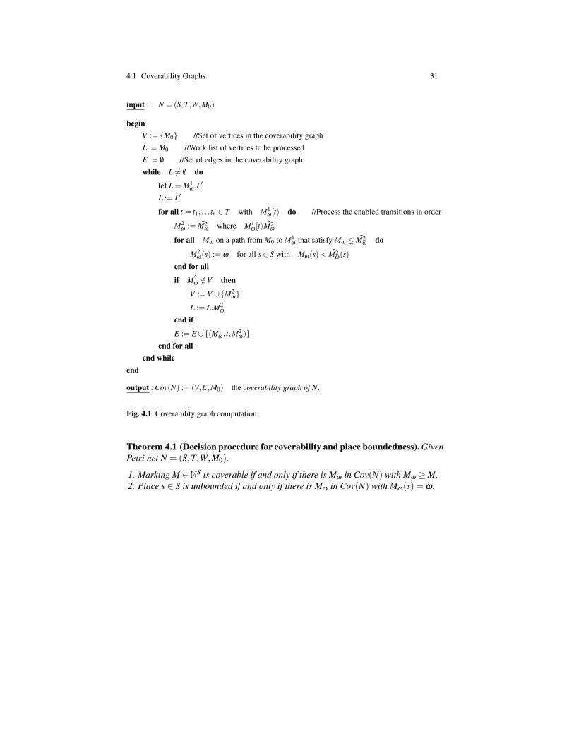
ω , s ∈ S, and t ∈ T .The coverability graph is computed (and defined) by the algorithm in Figure 4.1.
It introduces ω whenever a path strictly increases the token count. To make theoutcome of the computation deterministic, we use a FIFO buffer for the work listand an ordering on the transitions. Without this restriction, the resulting coverabilitygraph would depend on the processing order for markings and transitions.
Lemma 4.1 (Finiteness). For every Petri net N, Cov(N) is finite.
The proof bears similarities to the decision procedure for boundedness discussed inSection 1.2. To turn coverability graphs into a decision procedure for coverability,we need an equivalence of the following form. Marking M is coverable in N if andonly if there is Mω ∈ Cov(N) with M ≤Mω . The next lemmas provide the requiredimplications.
Lemma 4.2 (From N to Cov(N)). Consider Petri net N = (S,T,W,M0) and a tran-sition sequence σ ∈ T ∗ with M0[σ〉M for some M ∈R(N). Then there is a σ -labelledpath M0
σ−→Mω in Cov(N) that leads to Mω ≥M.
Thus, if a marking M is coverable in N then there is a larger marking Mω ≥ M inthe coverability graph. The following lemma states the reverse. Larger markings inthe coverability graph indeed indicate coverability in N.
Lemma 4.3 (From Cov(N) to N). Consider Petri net N = (S,T,W,M0). For everyMω ∈ Cov(N) and every k ∈ N there is a marking M ∈ R(N) with M(s) ≥ k for alls ∈Ω(Mω) and M(s) = Mω(s) for all s ∈ S\Ω(Mω).
The lemma states that the number of tokens on ω-marked places can exceed anybound k ∈N. The remaining places receive the exact token count as it is required bythe given marking Mω . The proof exploits the fact that sequences which introduceω-entries in the coverability graph can be repeated arbitrarily. Consider
M0τ−→M1
ω
σ−→M2ω with M1
ω M2ω .
By repeating σ , an arbitrary token count can be generated on the places s ∈ S withM1
ω(s)< M2ω(s). The proof is by induction on the length of the shortest path leading
to Mω . It requires some effort in case a new ω is introduced in the induction step.
4.1 Coverability Graphs 31
input : N = (S,T,W,M0)
beginV := M0 //Set of vertices in the coverability graph
L := M0 //Work list of vertices to be processed
E := /0 //Set of edges in the coverability graph
while L 6= /0 do
let L = M1ω .L′
L := L′
for all t = t1, . . . tn ∈ T with M1ω [t〉 do //Process the enabled transitions in order
M2ω := M2
ω where M1ω [t〉M2
ω
for all Mω on a path from M0 to M1ω that satisfy Mω M2
ω do
M2ω (s) := ω for all s ∈ S with Mω (s)< M2
ω (s)
end for all
if M2ω /∈V then
V :=V ∪M2ω
L := L.M2ω
end if
E := E ∪(M1ω , t,M
2ω )
end for allend while
end
output : Cov(N) := (V,E,M0) the coverability graph of N.
Fig. 4.1 Coverability graph computation.
Theorem 4.1 (Decision procedure for coverability and place boundedness). GivenPetri net N = (S,T,W,M0).
1. Marking M ∈NS is coverable if and only if there is Mω in Cov(N) with Mω ≥M.2. Place s ∈ S is unbounded if and only if there is Mω in Cov(N) with Mω(s) = ω .


Part IINetwork Protocols and Lossy Channel
Systems

Network protocols define the interaction among finite state components that com-municate asynchronously by package transfer. We introduce a corresponding modelof lossy channel systems and investigate algorithms for the automatic verificationof network protocols. Decidability of the analysis follows from monotonicity of themodels’ behaviour with respect to an ordering on the configurations. We extend thisinsight towards a theory of well structured transition systems.

Chapter 5Introduction to Lossy Channel Systems
Abstract Lossy Channel Systems
Lossy channel systems (LCS) formalize network protocols like the alternating bitprotocol or more general sliding window protocols that are located at the datalink layer of the ISO OSI reference model. In recent developments, LCS have alsoproven adequate for modelling programs running on relaxed memory models liketotal store ordering used in x86 processors.
Technically, LCS are finite state programs that communicate via asynchronousmessage transfer over unbounded FIFO channels. Without restrictions, such a modelof channel systems is Turing complete. Channels immediately reflect the tape of aTuring machine. The restriction we impose is inspired by the following observationabout the application domain of our analysis. Network protocols are designed tooperate correctly in the presence of package loss. Therefore, a weaker model withunreliable channels should be sufficient for their verification. Lossy channel systemsformalize unreliability by lossiness: channels may drop packages at any moment.This weakness indeed yields decidability of the resulting model.
5.1 Syntax and Semantics
Definition 5.1 (Lossy Channel Systems). A lossy channel system (LCS) is a tupleL = (Q,q0,C,M,→) where Q is a finite set of states with initial state q0 ∈Q. More-over, C is a finite set of channels over which we transfer messages in the finite setM. Transitions in→⊆ Q×OP×Q perform operations in OP :=C×!,?×M.
35

36 5 Introduction to Lossy Channel Systems
A transition (q1,op,q2) ∈ →, typically denoted by q1op−→ q2 yields a change in the
control state from q1 to q2 while performing operation op. A send operation c!a inOP appends message a to the current content of channel c. A receive operation c?a∈OP removes message a from the head of channel c. Therefore, the two operationsindeed define a FIFO channel.
In our examples, we often represent LCS by several automata. This matches theabove formal definition by taking as set of states the Cartesian product of the statesin the single automata. The initial state is the tuple of initial states. Every transitionsrepresents the state change in a single automaton.
Like every automaton model, the semantics of LCS relies on a notion of stateat runtime. For LCS, they are called configurations and should be understood asanalogue of markings in Petri nets.
Definition 5.2 (Configuration). Let L = (Q,q0,C,M,→). A configuration of L is apair γ = (q,W ) ∈Q×M∗C. It consists of a state q ∈Q and a function W ∈M∗C thatassigns to each channel c ∈C a finite word W (c) ∈M∗. The initial configuration ofL is γ0 := (q0,ε) where ε assigns the empty word (ε) to every channel.
Transitions change the channel content. We capture this by update operations onvectors of words. Lossiness is formalized by an ordering on configurations. For thedefinition of this ordering, we first compare words by Higman’s subword ordering. Itsets u∗ v if u is a not necessarily contiguous subword of v. With a componentwisedefinition, we lift the ordering to vectors of words, W1 ∗ W2. For configurations,we pose the additional requirement that the states coincide.
Definition 5.3 (Updates and on configurations). Updates take the form [c := x]with c ∈C and x ∈M∗. They are applied to channel contents W ∈M∗C. The resultof this application is a new content W [c := x] ∈M∗C defined by W [c := x](c) := xand W [c := x](c′) :=W (c′) for all c′ 6= c with c′ ∈C.
For the definition of the subword ordering ∗⊆M∗×M∗, let u = u1 . . .um and v =v1 . . .vn in M∗. We have u∗ v if there are indices 1≤ i1 < .. . < im ≤ n with u j = vi j
for all 1≤ j≤m. For W1,W2 ∈M∗C, we set W1∗W2 if W1(c)∗W2(c) for all c∈C.Finally, for configurations (q1,W1),(q2,W2)∈Q×M∗C we have (q1,W1) (q2,W2)if q1 = q2 and W1 ∗W2.
The semantics of LCS is defined in terms of transitions between configurations.
Definition 5.4 (Transition relation between configurations). Consider the LCSL = (Q,q0,C,M,→). It defines a transition relation→ ⊆ (Q×M∗C)× (Q×M∗C)between configurations as follows:
(q1,W )→ (q2,W [c :=W (c).m]) if q1c!m−−→ q2
(q1,W [c := m.W (c)])→ (q2,W ) if q1c?m−−→ q2
γ′1→ γ
′2 if γ
′1 γ1→ γ2 γ
′2
for some configurations γ1,γ2 ∈ Q×M∗C.
5.1 Syntax and Semantics 37
For a lossy transition (q1,W ′1)→ (q2,W ′2) that is derived with the third condition, wealready have a transition (q1,W1)→ (q2,W2) with W ′1 ∗ W1 and W2 ∗ W ′2. Intu-itively, the messages in W ′1 but outside W1 are lost immediately before the transitionand the messages in W2 but outside W ′2 are lost immediately afterwards.
Interestingly, for LCS the notions of reachability and coverability coincide. How-ever, as refer to coverability in the context of well structured transition systems, wedefine both notions.
Definition 5.5 (Reachability and Coverability). Let L = (Q,q0,C,M,→) be anLCS and γ1,γ2 ∈Q×M∗C. We say γ2 is reachable from γ1 if γ1→∗ γ2. The set of allconfigurations reachable from γ1 is R(γ1) := γ ∈ Q×M∗C | γ1→∗ γ. We denotethe reachable configurations of L by R(L) := R(γ0). Configuration γ2 is coverablefrom γ1 if there is γ ∈ R(γ1) with γ γ2.


Chapter 6Well Structured Transition Systems
Abstract Well Structured Transition Systems
6.1 Well Quasi Orderings
In computer science, quasi orderings that are not partial orderings result from syn-tactically different representations of semantically equivalent elements. To give anexample, let ≤ denote language inclusion. Then the regular expressions a+ b andb+a can be ordered by a+b≤ b+a as well as b+a≤ a+b. The terms, however,do not coincide.
Formally, a quasi ordering (qo) is a reflexive and transitive relation ≤ ⊆ A×A.We also call the pair (A,≤) a quasi ordering. In a qo, we write a > b for a≥ b andb a. Note that a ≥ b and b ≥ a need not imply a = b. In this case, ≤ is called apartial ordering. In the theory of well structured transition systems, so-called wellquasi orderings (wqos) play a key role. In a wqo, every infinite sequence containstwo comparable elements.
Definition 6.1 (Well quasi ordering). A qo (A,≤) is a well quasi ordering (wqo) iffor every infinite sequence (ai)i∈N in A there are indices i < j with ai ≤ a j.
We exploit the unavoidability of repetitions to establish termination of verificationalgorithms. Indeed, classical termination proofs rely on well founded relations thatdecrease with every transition. Recall that a quasi ordering (A,≤) is well foundedif it does not contain infinite sequences (ai)i∈N that strictly decrease, a0 > a1 > .. .Wqos additionally impose the absence of antichains. An antichain is a set B⊆ A ofincomparable elements, a 6≤ b for all a,b ∈ B.
Theorem 6.1 (Characterization of wqos). Consider the qo (A,≤). The followingstatements are equivalent:
39

40 6 Well Structured Transition Systems
1. (A,≤) is a wqo.2. Every infinite sequence (ai)i∈N in A contains an infinite non-decreasing subse-
quence (aϕ(i))i∈N with aϕ(i) ≤ aϕ(i+1) for all i ∈ N.3. There is no infinite strictly decreasing sequence and no infinite antichain in A.
Proof. (1)⇒ (2) Consider an infinite sequence (ai)i∈N in A. Take the subsequence(and(i))i∈N of elements that are not dominated by successors, i.e., for all and(i) thereis no a j with nd(i) < j and and(i) ≤ a j. The sequence has to be finite by the wellquasi ordering assumption. Let n := nd(k) be the maximal index in this sequence.Starting from n+ 1 one finds an infinite non-decreasing subsequence since everyelement after an is dominated by (≤) some successor.
(2)⇒ (3) By definition.
(3)⇒ (1) Consider an infinite sequence (ai)i∈N. We show that there are i < j withai ≤ a j. The idea is to descend strictly decreasing sequences and gather the leastelements in an antichain. By the well foundedness assumption and the absence ofinfinite antichains, the procedure terminates and finds two comparable elements.
Consider the first element a0. If there is a successor a j with a0 ≤ a j we aredone. Otherwise, we find the first successor aϕ(1) with a0 > aϕ(1). We repeat theargumentation for aϕ(1). If there is a successor a j with aϕ(1) ≤ a j, we found twocomparable elements. Otherwise, we find the first successor aϕ(2) with
a0 > aϕ(1) > aϕ(2).
The search eventually terminates because there are no infinite strictly decreasingsequences. Let aϕ(n0) be the element that has no successor a j with aϕ(n0) ≤ a j andno successor a j with aϕ(n0) > a j. Add aϕ(n0) as first element to an antichain.
We proceed with aϕ(n0)+1. Again we search for aϕ(n1) that has no successor a jwith aϕ(n1) ≤ a j and no successor a j with aϕ(n1) > a j. By construction
aϕ(n0) 6≤ aϕ(n1) and aϕ(n0) 6> aϕ(n1).
Hence, the set aϕ(n0),aϕ(n1) is an antichain of size two. Repeating the procedureindefinitely yields an infinite antichain. A contradiction to the assumption that noinfinite antichains exists. We have to find i < j with ai ≤ a j. ut
A reader familiar with Ramsey’s theorem will find a more elegant proof of the lastimplication (3)⇒ (1), in fact even of the stronger statement (3)⇒ (2). Ramsey’stheorem considers infinite complete graphs where the edges are labelled by finitelymany colors. It states that such a graph contains an infinite complete subgraph thatis labelled by a single color. To apply the theorem, note that an infinite sequence(ai)i∈N induces the infinite complete graph where the elements ai are the vertices.The edges are labelled by the relations ≤,>, incomparable. Let i< j and considerthe edge between ai and a j. We label it by ≤ if ai ≤ a j. We label it by > if ai > a j.Otherwise, we label it by incomparable. Ramsey’s theorem applies and yields aninfinite complete subgraph labelled by a single color. By the assumptions, the color

6.2 Upward and downward closed sets 41
cannot be > and not incomparable. Hence, we found an infinite non-decreasingsubsequence.
6.2 Upward and downward closed sets
In wqos, every set B contains finitely many minimal elements min(B). Minimalelements are interesting as they represent, in a precise way, so-called upward closedsets.
Definition 6.2 (Minimal elements). Let (A,≤) be a wqo and let B ⊆ A. A set ofminimal elements is a subset min(B) ⊆ B that contains for every b ∈ B an elementm ∈ min(B) with m≤ b and that is an antichain.
Lemma 6.1 (Existence and finiteness of minimal elements). Let (A,≤) be a wqoand B⊆ A. There is a finite set of minimal elements min(B).
Proof. To the contrary, assume there is no finite set of minimal elements. We forman infinite sequence (bi)i∈N starting with some b0 ∈B. As bi+1 we choose an elementthat is no larger than any predecessor, b j 6≤ bi+1 for all 0 ≤ j ≤ i. Such an elementexists, otherwise we can construct a finite set of minimal elements from b0, . . . ,bi.The resulting infinite sequence (bi)i∈N violates the wqo assumption. ut
Note that min(B) need not be unique as antisymmetry is missing. With an algorith-mic point of view, the lemma can be understood as follows. Sets min(B) of minimalelements are good candidates for finite representations of infinite sets. The sets thatcan be captured precisely by their minimal elements are upward closed.
Definition 6.3 (Upward and downward closure). Let (A,≤) be a wqo. A set I ⊆ Ais upward closed if x ∈ I and a ≥ x for a ∈ A implies a ∈ I. The upward closure ofa set B ⊆ A is B ↑ := a ∈ A | a ≥ b for some b ∈ B. Similarly, a set D ⊆ A isdownward closed if x∈D and a≤ x for a∈ A implies a∈D. The downward closureof B⊆ A is B↓ := a ∈ A | a≤ b for some b ∈ B.
Lemma 6.2 (Representation of upward closed sets by minimal elements). Let(A,≤) be a wqo and consider an upward closed set I ⊆ A. Let min(I) be a finite setof minimal elements. Then I = min(I)↑.
The decision procedure for coverability in wsts deals with increasing sequences ofupward closed sets. The wqo assumption guarantees that these sequences stabilize,which in turn ensures termination of the algorithm.
Theorem 6.2 (Chains of upward closed sets stabilize). Consider a qo (A,≤). Thefollowing statements are equivalent:
1. (A,≤) is a wqo.2. For every infinite increasing sequence I0 ⊆ I1 ⊆ I2 ⊆ . . . of upward closed sets
I j ⊆ A there is a k ∈ N with Ik = Ik+1.

42 6 Well Structured Transition Systems
3. For every infinite increasing sequence I0 ⊆ I1 ⊆ I2 ⊆ . . . of upward closed setsI j ⊆ A there is an l ∈ N with Il = Il+1 = Il+2 = . . .
Proof. (1)⇒ (2) Towards a contradiction, assume there is an infinite sequenceI0 ( I1 ( I2 ( . . . Then there are elements a0 ∈ I1 \ I0, a1 ∈ I2 \ I1, a2 ∈ I3 \ I2, . . .Since the sets I j are upward closed, we can conclude ai 6≤ a j for all i, j ∈ N withi < j. The sequence (ai)i∈N violates the wqo assumption.
(2)⇒ (3) Again we proceed by contradiction and assume (3) does not hold. Thismeans there is an infinite sequence I0 ⊆ I1 ⊆ I2 ⊆ . . . so that for every k ∈ N thereis k1 with k < k1 and Ik ( Ik1 . For k1 there is again a later k1 < k2 with Ik1 ( Ik2 etc.We single out this infinite strictly increasing subsequence.
Ik ( Ik1 ( Ik2 ( . . .
By assumption (2), the sequence contains Ik j = Ik j+1 . A contradiction.
(3)⇒ (1) Consider sequence (ai)i∈N in A. We define a sequence of upward closedsets: I0 := a0↑, I1 := a0,a1↑, etc. Since I0 ⊆ I1 ⊆ . . . there is a smallest l ∈ Nwith Il = Il+1 = . . . This means there is j < l +1 with a j ≤ al+1. ut
6.3 Constructing well quasi orderings
The importance of well structured transition systems stems from the fact that manysets are well quasi ordered. This in turn is based on the observation that wqos can becomposed into new ones. We present an algebraic toolkit to derive the wqos neededin this lecture. The list is not complete. We skip Kruskal’s theorem on a well quasiordering on trees and also the graph minor theorem.
Every finite set is well quasi ordered by equality. Moreover, the natural numbersare well quasi ordered by ≤.
Lemma 6.3. If A is finite, then (A,=) is a wqo. Moreover, (N,≤) is a wqo.
Well quasi orderings are stable under Cartesian products.
Lemma 6.4. Consider two wqos (A,≤A) and (B,≤B). Then (A×B,≤A×B) is a wqowhere (a1,b1)≤A×B (a2,b2) if a1 ≤A a2 and b1 ≤B b2.
Proof. Consider an infinite sequence (ai,bi)i∈N in A×B. As (ai)i∈N is an infinitesequence in A and A is a wqo by the assumption, there is (Theorem 6.1) an infinitenon-decreasing subsequence (aϕ(i))i∈N with aϕ(i) ≤A aϕ(i+1) for all i ∈ N.
Consider the sequence (aϕ(i),bϕ(i))i∈N. As (bϕ(i))i∈N is an infinite sequence inB, by the wqo assumption there are i < j with bϕ(i) ≤B bϕ( j). By the definition ofsubsequences, i < j implies ϕ(i)< ϕ( j). So we found indices ϕ(i)< ϕ( j) with
aϕ(i) ≤A aϕ( j) and bϕ(i) ≤B bϕ( j).
We conclude (aϕ(i),bϕ(i))≤A×B (aϕ( j),bϕ( j)) as required. ut

6.4 Well Structured Transition Systems 43
Words can be understood as an unbounded version of Cartesian products. Higmanhas shown that also words are well quasi ordered (by the subword relation).
Lemma 6.5 (Higman 1952). If (A,≤) is a wqo, so is (A∗,≤∗). Here, u ≤∗ v withu = u1 . . .um and v = v1 . . .vn if there are 1≤ i1 < .. . < im ≤ n with u j ≤ vi j for all1≤ j ≤ m.
Proof. To the contrary, assume there are infinite sequences that are bad, i.e., thatdo not contain comparable elements. We rely on a combinatorial construction toderive the contradiction. It forms an infinite bad sequence (ui)i∈N that is particularlysmall as follows. Select the shortest word u0 that starts a bad sequence. Assume weconstructed the sequence u0, . . . ,un. We then append the shortest word un+1 so thatthe result u0, . . . ,un+1 still forms a prefix of a bad sequence.
The infinite sequence (ui)i∈N is bad. Let ui = ai.vi with ai ∈ A and vi ∈ A∗. By thewell quasi ordering assumption on A and Theorem 6.1, sequence (ai)i∈N containsan infinite non-decreasing subsequence (aϕ(i))i∈N. Consider now the sequence
u0, . . . ,uϕ(0)−1,vϕ(0),vϕ(1), . . .
Since vϕ(0) is strictly shorter than uϕ(0), the sequence has to be good (otherwise wewould have selected vϕ(0) instead of uϕ(0)). This means, there are two comparableelements. They cannot be among u0, . . . ,uϕ(0)−1, otherwise the sequence (ui)i∈Nwould have been good. Moreover, the ordering cannot be between ui and vϕ( j).Otherwise, we had ui ≤∗ vϕ( j) ≤∗ uϕ( j) and so ui ≤∗ uϕ( j). Again a contradictionto the assumption that (ui)i∈N is bad. Hence, we have vϕ(i) ≤∗ vϕ( j) with i < j.By monotonicity, this means ϕ(i) < ϕ( j). But since also aϕ(i) ≤ aϕ( j), we deriveuϕ(i) = aϕ(i).vϕ(i) ≤∗ aϕ( j).vϕ( j) = uϕ( j). A contradiction. ut
6.4 Well Structured Transition Systems
Well structured transition systems are a framework for the automatic verificationof infinite state systems. The concept was found independently by Alain Finkel(Cachan) and Parosh Abdulla (Uppsala) when they worked on generalizations ofdecision procedures that were known for particular models. Finkel strived for anextension of coverability graphs in order to decide termination and boundednessproblems. Abdulla was interested in coverability and simulation problems for lossychannel systems.
Technically, wsts are (usually infinite) transition systems where the configura-tions are equipped with a well quasi ordering. This wqo has to be compatible withthe transitions, i.e., larger configurations can imitate the transitions of smaller ones.Imitation is formalized by so-called simulation relations.
Definition 6.4 (Well structured transition system (wsts), simulation relation).A transition systems is a triple TS = (Γ ,γ0,→) with a (typically infinite) set ofconfigurations Γ , an initial configuration γ0 ∈ Γ , and a transition relation → ⊆

44 6 Well Structured Transition Systems
Γ ×Γ . The transition system is well structured if there is ≤ ⊆ Γ ×Γ that is a wqoand a simulation relation. We also write TS = (Γ ,γ0,→,≤) for a wsts.
Recall that ≤ ⊆ Γ ×Γ is a simulation (relation) if for all γ1,γ2,γ3 ∈ Γ withγ1→ γ2 and γ1 ≤ γ3 there is γ4 ∈ Γ with γ3→ γ4 and γ2 ≤ γ4.
With the ordering ⊆ (Q×M∗C)× (Q×M∗C) from Definition 5.3, lossy channelsystems are indeed well structured.
Theorem 6.3 (Lcs are wsts). Consider the lcs L = (Q,q0,C,M,→). The transitionsystem (Q×M∗C,γ0,→,) is well structured.
For the proof, it remains to be shown that is a wqo and a simulation.
6.5 Abdulla’s Backwards Search
Our goal is to decide coverability in lossy channel systems. Recall that configuration(q,W ) ∈ Q×M∗C is coverable in L = (Q,q0,C,M,→) if there is a configurationγ ∈ R(L) with γ (q,W ). With upward closed sets, the problem can be rephrasedas follows. Is the upward closed set (q,W )↑ reachable?
We present an algorithm that solves reachability of upward closed sets in a wsts.Formally, the problem takes as input a wsts TS=(Γ ,γ0,→,≤) and an upward closedset I ⊆ Γ . The question is whether I is reachable from γ0. More precisely, is therean element γ ∈ I with γ0→∗ γ . We first discuss the general decision procedure forwsts and then instantiate it to lossy channel systems.
Before we plunge into the details, we sketch the procedure and mention the keyarguments. The idea is to perform the reachability analysis backwards. We start withthe set I0 = I of interest. Then we compute the set of configurations I1 that reach Iin at most one step. We continue with the configurations I2 that lead to I in up totwo steps and so on. The procedure allows us to reformulate reachability as follows.The set I is reachable form γ0 if and only if γ0 ∈
⋃j≥0 I j.
The sets I j can be shown to be upward closed. Moreover, they form an infinitechain I0 ⊆ I1 ⊆ I2 ⊆ . . . Therefore, Theorem 6.2 applies and states that the chainstabilizes in some k ∈ N: Ik = Ik+1 = Ik+2 = . . . With reference to the infinite unionabove, we get
⋃j≥0 I j = Ik. This equation suggests the following procedure to decide
upward closed reachability:
• Generate the sequence of upward closed sets I0 ⊆ I1 ⊆ I2 ⊆ . . .• Check for stabilization, Ik = Ik+1.• If the sequence stabilized, check for membership γ0 ∈ Ik.
The problem is that the sets I j are infinite. This means neither equality Ik = Ik+1nor membership γ0 ∈ Ik can be checked algorithmically without further assumptionson the I j. The solution is to represent these sets symbolically by means of minimalelements M j and exploit the equation I j = M j ↑. This allows us to store and updateonly finite sets.
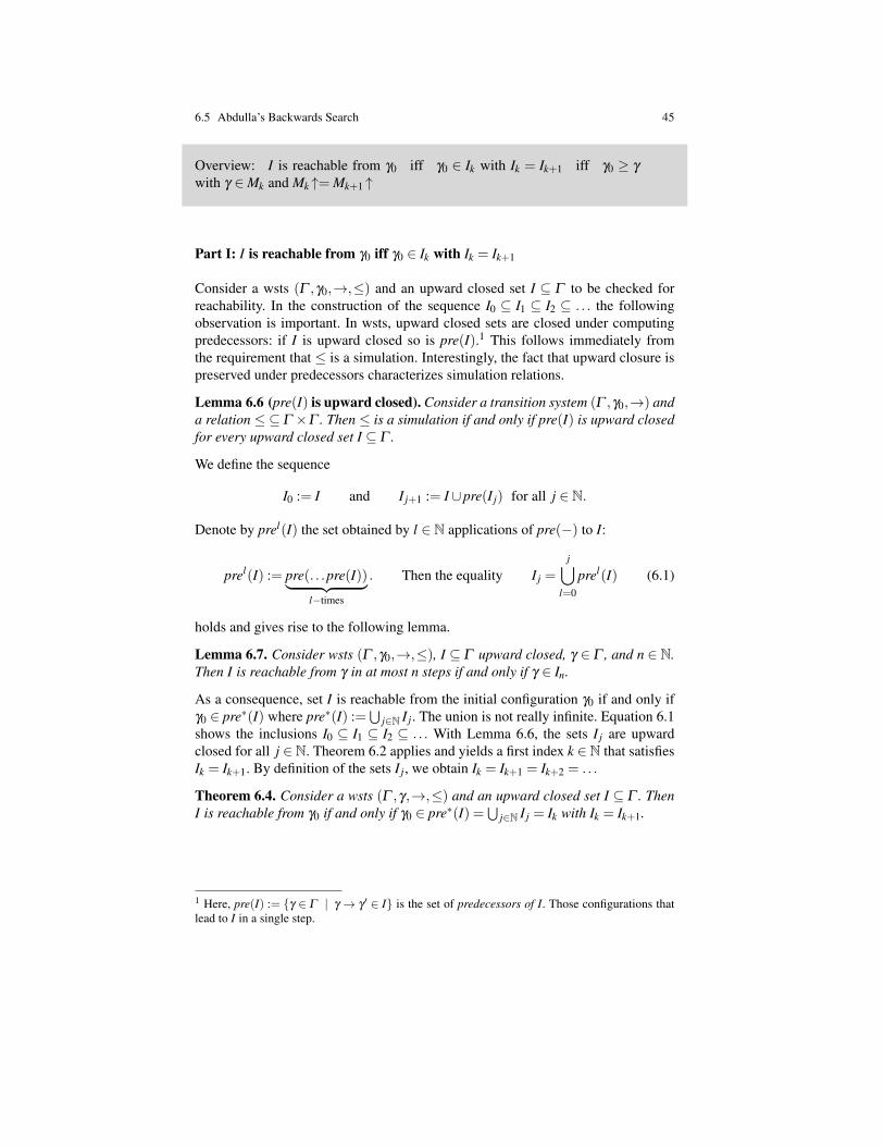
6.5 Abdulla’s Backwards Search 45
Overview: I is reachable from γ0 iff γ0 ∈ Ik with Ik = Ik+1 iff γ0 ≥ γ
with γ ∈Mk and Mk ↑= Mk+1 ↑
Part I: I is reachable from γ0 iff γ0 ∈ Ik with Ik = Ik+1
Consider a wsts (Γ ,γ0,→,≤) and an upward closed set I ⊆ Γ to be checked forreachability. In the construction of the sequence I0 ⊆ I1 ⊆ I2 ⊆ . . . the followingobservation is important. In wsts, upward closed sets are closed under computingpredecessors: if I is upward closed so is pre(I).1 This follows immediately fromthe requirement that ≤ is a simulation. Interestingly, the fact that upward closure ispreserved under predecessors characterizes simulation relations.
Lemma 6.6 (pre(I) is upward closed). Consider a transition system (Γ ,γ0,→) anda relation ≤ ⊆ Γ ×Γ . Then ≤ is a simulation if and only if pre(I) is upward closedfor every upward closed set I ⊆ Γ .
We define the sequence
I0 := I and I j+1 := I∪pre(I j) for all j ∈ N.
Denote by prel(I) the set obtained by l ∈ N applications of pre(−) to I:
prel(I) := pre(. . .pre(I))︸ ︷︷ ︸l−times
. Then the equality I j =j⋃
l=0
prel(I) (6.1)
holds and gives rise to the following lemma.
Lemma 6.7. Consider wsts (Γ ,γ0,→,≤), I ⊆ Γ upward closed, γ ∈ Γ , and n ∈ N.Then I is reachable from γ in at most n steps if and only if γ ∈ In.
As a consequence, set I is reachable from the initial configuration γ0 if and only ifγ0 ∈ pre∗(I) where pre∗(I) :=
⋃j∈N I j. The union is not really infinite. Equation 6.1
shows the inclusions I0 ⊆ I1 ⊆ I2 ⊆ . . . With Lemma 6.6, the sets I j are upwardclosed for all j ∈N. Theorem 6.2 applies and yields a first index k ∈N that satisfiesIk = Ik+1. By definition of the sets I j, we obtain Ik = Ik+1 = Ik+2 = . . .
Theorem 6.4. Consider a wsts (Γ ,γ,→,≤) and an upward closed set I ⊆ Γ . ThenI is reachable from γ0 if and only if γ0 ∈ pre∗(I) =
⋃j∈N I j = Ik with Ik = Ik+1.
1 Here, pre(I) := γ ∈ Γ | γ → γ ′ ∈ I is the set of predecessors of I. Those configurations thatlead to I in a single step.
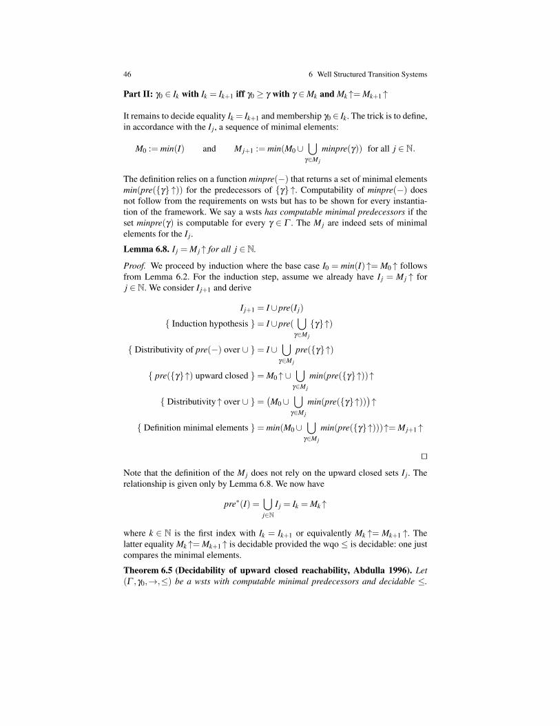
46 6 Well Structured Transition Systems
Part II: γ0 ∈ Ik with Ik = Ik+1 iff γ0 ≥ γ with γ ∈Mk and Mk ↑= Mk+1 ↑
It remains to decide equality Ik = Ik+1 and membership γ0 ∈ Ik. The trick is to define,in accordance with the I j, a sequence of minimal elements:
M0 := min(I) and M j+1 := min(M0∪⋃
γ∈M j
minpre(γ)) for all j ∈ N.
The definition relies on a function minpre(−) that returns a set of minimal elementsmin(pre(γ ↑)) for the predecessors of γ ↑. Computability of minpre(−) doesnot follow from the requirements on wsts but has to be shown for every instantia-tion of the framework. We say a wsts has computable minimal predecessors if theset minpre(γ) is computable for every γ ∈ Γ . The M j are indeed sets of minimalelements for the I j.
Lemma 6.8. I j = M j ↑ for all j ∈ N.
Proof. We proceed by induction where the base case I0 = min(I)↑= M0 ↑ followsfrom Lemma 6.2. For the induction step, assume we already have I j = M j ↑ forj ∈ N. We consider I j+1 and derive
I j+1 = I∪pre(I j)
Induction hypothesis = I∪pre(⋃
γ∈M j
γ↑)
Distributivity of pre(−) over ∪ = I∪⋃
γ∈M j
pre(γ↑)
pre(γ↑) upward closed = M0 ↑ ∪⋃
γ∈M j
min(pre(γ↑))↑
Distributivity↑ over ∪ =(M0∪
⋃γ∈M j
min(pre(γ↑)))↑
Definition minimal elements = min(M0∪⋃
γ∈M j
min(pre(γ↑)))↑= M j+1 ↑
ut
Note that the definition of the M j does not rely on the upward closed sets I j. Therelationship is given only by Lemma 6.8. We now have
pre∗(I) =⋃j∈N
I j = Ik = Mk ↑
where k ∈ N is the first index with Ik = Ik+1 or equivalently Mk ↑= Mk+1 ↑. Thelatter equality Mk ↑= Mk+1 ↑ is decidable provided the wqo ≤ is decidable: one justcompares the minimal elements.
Theorem 6.5 (Decidability of upward closed reachability, Abdulla 1996). Let(Γ ,γ0,→,≤) be a wsts with computable minimal predecessors and decidable ≤.

6.5 Abdulla’s Backwards Search 47
Consider the upward closed set I ⊆ Γ given by its minimal elements min(I). Then itis decidable whether I is reachable from γ0.
Proof. The algorithm computes the sequence of minimal elements as defined above.When it finds Mk ↑= Mk+1 ↑, it terminates as now pre∗(I) = Mk ↑. By Theorem 6.4,γ0 reaches I iff γ0 ≥ γ with γ ∈Mk. ut
To instantiate the algorithm to LCS, we need a suitable minpre(−) function. LetL = (Q,q0,C,M,→). We take as minpre(q2,W2) := min(T ), where T is the smallestset so that
(q1,W1) ∈ T if q1c!m−−→ q2 and W2 =W1[c :=W1.m]
(q1,W2) ∈ T if q1c!m−−→ q2 and the last element of W2(c) 6= m (or W2(c) is empty)
(q1,W1) ∈ T if q1c?m−−→ q2 and W1 =W2[c := m.W2(c)]
Lemma 6.9. Consider LCS L = (Q,q0,C,M,→) and configuration γ ∈ Q×M∗C.Then minpre(γ) = min(pre(γ↑)).
One may be skeptical about (q1,W2) ∈ T if q1c!m−−→ q2 and the last element of W2(c)
is different from m. We have (q1,W2)→ (q2,W2[c :=W2(c).m])≥ (q2,W2). Hence,(q1,W2) ∈ pre((q2,W2)↑).
There is no configuration (q1,W ′2) with W ′2 ≺∗W2 (in case last W2(c) 6= m). Oneadds m in order to take the transition. The letter is lost to get W2(c). Since only asingle letter can be added, W2(c) cannot be constructed from W ′2(c)≺∗W2(c).


Chapter 7Simple Regularity and Symbolic ForwardAnalysis
Abstract Symbolic forward analysis of lossy channel systems
7.1 Simple Regular Expressions and Languages
Recall that the regular expressions over an alphabet M are defined by finite unions,concatenation, and Kleene star of single letters:
re ::= /0 | ε | a | re1 + re2 | re1.re2 | re∗ where a ∈M.
Regular expressions re denote languages L (re)⊆M∗ in the standard way:
L ( /0) := /0 L (re1 + re2) := L (re1)∪L (re2)
L (ε) := ε L (re1.re2) := L (re1).L (re2)
L (a) := a L (re∗) := L (re)∗ :=⋃j∈N
L (re) j
Here, L (re) j denotes j ∈ N concatenations of L (re) where we fix L (re)0 := ε .Simple regular expressions are designed to represent languages that are downwardclosed wrt. Higman’s subword ordering ∗. Therefore, every occurrence of a letteralso offers the choice of loss.
Definition 7.1 (Simple regular expression). Consider some underlying alphabetM. Atomic expressions e allow for choices among letters and form the base case.They are concatenated to products p. Simple regular expressions (sres) r are thenchoices among products:
e ::= (a+ ε) | (a1 + . . .+am)∗ p ::= ε | e.p r ::= /0 | p+ r
49

50 7 Simple Regularity and Symbolic Forward Analysis
where a,a1, . . . ,am ∈M. A language L ⊆M∗ is simple regular if there is a simpleregular expression r with L = L (r).
Haines showed that downward closed languages are regular. We first establish thisresult and then sharpen it as follows. Downward closed languages are precisely thelanguages represented by sres.
Theorem 7.1 (Haines ’69). Let L ⊆M∗ be any language. Then L ↓ is regular.
Proof. Since L ↓ is downward closed, the complement L ↓ is upward closed. SinceHigman’s ordering ∗ is a wqo, this upward closed language can be represented byits (finitely many) minimal elements:
L ↓ = min(L ↓)↑ =⋃
w∈min(L↓)
w↑ . (7.1)
Note that the upward closure of a word w = w1 . . .wn is the language
w↑ = y ∈M∗ | w∗ y = L (M∗.w1.M∗ . . .M∗.wn.M∗)
where M∗ denotes the choice Σm∈Mm. This means w↑ is regular. Since min(L ↓)is finite by Lemma 6.1 and since regular languages are closed under finite unions, weconclude with Equation 7.1 that L ↓ is regular. Regular languages are also closedunder complementation, so L↓= L ↓ is regular. ut
The result is indeed surprising. If we define the language of a Turing machine tocontain all sequences of transitions that lead to a halting state, we get that L (TM)↓is regular. This in turn means that the downward closure of languages cannot becomputable in general. In the example of Turing machines, we would obtain
TM halts iff L (TM)↓6= /0 iff ε ∈L (TM)↓ .
So there is no algorithm to compute a representation of L (TM)↓ (more precisely,no representation which allows us to evaluate emptiness or membership of ε).
There are interesting classes of languages for which the downward closure iscomputable. Van Leeuwen has shown in 1978 that the downward closure of contextfree languages is effectively computable. For Petri nets, the problem remained openuntil 2010 when it was solved positively by Habermehl, Wimmel, and the author.Establishing such computability results is a beautiful theoretical challenge that findsapplications in decidability results for asynchronous hardware. Indeed, consider ashared memory architecture with a writer and a reader. The reader always sees thedownward closure of the writers actions. If the reader process is slower than thewriter, it may miss intermediary instructions. It was Ahmed Bouajjani who realizedthis applications of downward closed languages in modelling and verification.
Theorem 7.2 (Bouajjani ’98). Language L is downward closed if and only if it issimple regular.

7.1 Simple Regular Expressions and Languages 51
Proof. For the if direction, recall that simple regularity means L = L (r) for somesre r. Therefore, an induction along the structure of sres is sufficient that showsL (r) is downward closed for all sres.
For the only if direction, we apply Haines’ theorem and obtain
L = L =⋃
w∈min(L )
w↑ =⋂
w∈min(L )
w↑. (7.2)
To find an sre for w↑, we take a detour and represent w↑ by a finite automaton.This allows us to apply the standard construction for complementation, which hintsto the required expression. Let w = w1 . . .wn with M as underlying alphabet. Thelanguage w↑ is accepted by
q0
M
Aw↑
q1
M
. . . . . .
qn
M
w1 w2 wn
The M labelled loops denote |M| loops, one for each letter in M. We determinize theautomaton with the powerset construction of Rabin and Scott. Switching then finaland non-final states yields an automaton for the complement language:
q0
M \w1
det(Aw↑)
q0,q1
M \w2
. . . . . .
q0, . . . ,qn−1
M \wn
q0, . . . ,qn
M
w1 w2 wn−1 wn
The automaton operations are known to reflect the operations on languages. Thus,the language of det(Aw↑) is as desired:
L (det(Aw↑)) = L (det(Aw↑)) = L (Aw↑) = w↑.
The language is characterized by the sre
(M \w1)∗.(w1 + ε).(M \w2)∗.(w2 + ε) . . .(wn−1 + ε).(M \wn)∗
According to Equation 7.2, we need an sre for the intersection⋂
w∈min(L ) w↑.On automata, this intersection is reflected by a parallel composition
∏w∈min(L )
det(Aw↑).
The result is an, up to loops, acyclic automaton. We decompose it into its maximalpaths and reuse the above construction. ut

52 7 Simple Regularity and Symbolic Forward Analysis
7.2 Inclusion among simple regular languages
We intend to use sres to represent sets of configurations in a lossy channel system.More precisely, we develop a concept of symbolic configurations (q,R) where Ris a function that assings to each channel c an sre R(c). Based on such symbolicconfigurations, we again develop a fixed point algorithm of the form
I0 ⊆ I1 ⊆ I2 ⊆ . . . until Ik+1 = Ik for some k ∈ N.
As the sequence already is increasing, we only need to check Ik+1 ⊆ Ik. Thiscalls for an inclusion check L (r1) ⊆L (r2) among simple regular languages. Thefollowing result is key to making this inclusion check efficient. It states that we onlyneed to compare products with products.
Lemma 7.1. Consider a product p and an sre r = p1 + . . .+ pk. If L (p) ⊆L (r)then L (p)⊆L (pi) for some 1≤ i≤ k.
Proof. The proof approach is interesting. We devise a single word y ∈L (p) thatis demanding enough so as to ensure inclusion of the full language L (p). Moreprecisely, the word will guarantee that
y ∈L (pi) implies L (p)⊆L (pi)
for every product pi with 1≤ i≤ k. This proves the lemma as
y ∈ L (p) ⊆ L (r) =k⋃
i=1
L (pi)
yields y ∈ L (pi) for some 1 ≤ i ≤ k. With the above implication, we concludeL (p)⊆L (pi) for this pi. All that remains is to give the construction of y.
Let p = e1 . . .en and let j be the maximal number of atomic expressions in theproducts in r = p1 + . . .+ pk. The goal is to enforce L (p) ⊆L (pi) if y ∈L (pi).We set y = y1 . . .yn with
yi := a if ei = (a+ ε) yi := (a1 . . .am)j+1 if ei = (a1 + . . .+am)
∗.
This means we have a word for every atomic expression. For a choice ei = (a+ ε)we select yi = a to demand the occurrence of letter a. For ei = (a1 + . . .am)
∗ weapply the pigeonhole principle. Let the longest product in r be e′1 . . .e
′j. We choose
yi = (a1 . . .am)j+1. This means at least two iterations of a1 . . .am have to be in the
language of a same expression, (a1 . . .am)2 ∈L (e′l) for some 1≤ l≤ j. This implies
e′l = (. . .+ a1 + . . .+ am)∗ and guarantees L (ei) ⊆ L (e′l). Inclusion of the full
product p = e1 . . .en iterates the argument for single expressions. ut
We now develop a recursive algorithm that checks inclusion among products inlinear time. If one of the products is the empty word, we have L (ε) ⊆L (p) forevery product p and L (p) 6⊆L (ε) for all p 6= ε . For atomic expressions, we have

7.3 Computing the Effect of Transitions 53
L (a+ ε)⊆L ((a1 + . . .+am)∗) if a ∈ a1, . . . ,am
L ((a1 + . . .+am)∗)⊆L ((b1 + . . .+bn)
∗) if a1, . . . ,am ⊆ b1, . . . ,bn.
It remains to set up the recursion for proper products e1.p1 and e2.p2. We returnL (e1.p1)⊆L (e2.p2) if one of the following holds:
L (e1) 6⊆L (e2) and L (e1.p1)⊆L (p2)
L (e1) = L (e2) = L (a+ ε) and L (p1)⊆L (p2)
L (e1)⊆L (e2) = L ((a1 + . . .+am)∗) and L (p1)⊆L (e2.p2).
Lemma 7.2. Inclusion among products can be checked in linear time.
To check inclusion L (p1 + . . .+ pm)⊆L (p′1 + . . .+ p′n) among sres, we compareeach product pi with every product p′j until we find L (pi) ⊆ L (p′j). This localcheck among products is sufficient according to Lemma 7.1.
Lemma 7.3. Inclusion among sres can be checked in quadratic time.
7.3 Computing the Effect of Transitions
The result of applying an operation like c!a to an sre r should again be an sre. Weshow how to compute this sre. In the next section, we obtain a similar computabilityresult for the application of iterated sequences of operations.
We fix the channel c to which we apply the operations and write !a and ?a insteadof c!a and c?a. Let M be the alphabet of messages that are sent and received. Wedefine the effect of performing a send operation !a on L ⊆M∗ to be the languageL⊕!a := y ∈ M∗ | y = x.a for some x ∈ L . Similarly, the effect of receivingfrom L is defined by L⊕?a := y∈M∗ | x = a.y for some x∈L . The languagesL we are concerned with are represented by sres r. The following lemma showshow to compute an sre that represents L (r)⊕op.
Lemma 7.4. Consider an sre r and an operation op∈!a,?a. There is an sre r⊕opwith L (r⊕op) = L (r)⊕op. Moreover, r⊕op can be computed in linear time.
Proof. We first consider products. For send operations, we set p⊕!a := p.(a+ ε).For receive operations, the base case is ε⊕?a := /0. In the induction step, we have
(e.p)⊕?a :=
e.p if e = (a1 + . . .+am)
∗ and a ∈ a1, . . . ,amp if e = (a+ ε)
p⊕?a otherwise.
This means the operation is applied to the remaining product p provided letter acannot be served by the first atomic expression e.

54 7 Simple Regularity and Symbolic Forward Analysis
For an sre r = p1 + . . .+ pk we set r⊕op := (p1⊕op)+ . . .+(pk⊕op) to applythe operation to all products. It is readily checked that language equality holds andthat r⊕op can be computed in time linear in the size of r. ut
7.4 Computing the Effect of Loops
Our goal is to accelerate the coverability analysis in lossy channel systems. The termacceleration means we determine the effect of arbitrary iterations of control loopsin a single computation, rather than calculating the effect of every transition.
Technically, a control loop is a sequence of transitions that starts and ends in asame state:
q0op1−−→ q1
op2−−→ . . .opn−−→ qn with q0 = qn.
We assume that all operations in ops = op1 . . .opn act on the same channel c.1 Themain contribution is an algorithm which, given an sre r and sequence ops, computesa new sre r⊕ops∗. The latter reflects the effect of arbitrary iterations of ops on r.
The key insight is that the effect of loops stabilizes. For every sre r and sequenceops, there is an n ∈ N that satisfies the following. The language obtained by at leastn iterations of ops on r is characterized by an sre r⊕ops≥n. As a consequence, theeffect of arbitrary iterations of ops on r can be captured by the sre
r⊕ops∗ := r+(r⊕ops)+ . . .+(r⊕opsn−1)+(r⊕ops≥n).
Theorem 7.3 (Bouajjani 1998). Consider product p and a sequence of operationsops. There is an n ∈ N and a product p⊕ops≥n so that either L (p⊕opsn) = /0 orL (p⊕ ops≥n) =
⋃j≥n L (p⊕ ops j). The value of n is linear in the size of p and
p⊕ops≥n can be computed in quadratic time.
Before we turn to the proof, we define notions that help us shorten the presentation.Consider a sequence ops of operations !a or ?a where a is in the alphabet M. Wedenote by ops? the subword of receive operations. Similarly, ops! yields the subwordof send operations. We assume the symbol of operation to be removed. So for ops =!a.?b.?c.!d we have ops? = b.c and ops! = a.d. We use M(ops?) and M(ops!) torestrict alphabet M to the letters in ops? and ops!, respectively.
We extend Higman’s ordering into two directions. We use the growing subwordordering x∗grow y with x,y ∈M∗ to indicate that there is m ∈N so that xm+1 ∗ ym.Not only does x ∗grow y imply x ∗ y. It indeed shows that y is large enough so asto accommodate several instances of x. If both words are iterated m+1 times, thenxm+1 fits into only m iterations of y. The (m+1)st iteration of y is left untouched bythe subword ordering. Ordering ∗grow can be checked in quadratic time.
If we iterate a control loop, ops can be understood as a cycle. Indeed, whenthe last operation opn in the control loop is reached, the word will continue with
1 If this is not the case, we first decompose ops into the subwords opsc for the single channels.
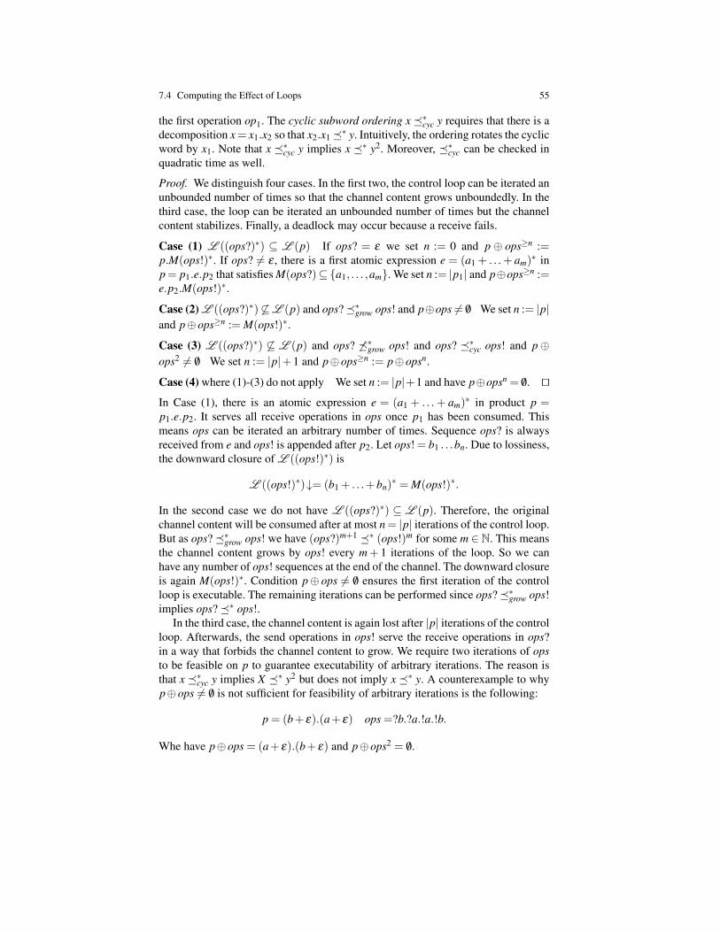
7.4 Computing the Effect of Loops 55
the first operation op1. The cyclic subword ordering x∗cyc y requires that there is adecomposition x= x1.x2 so that x2.x1∗ y. Intuitively, the ordering rotates the cyclicword by x1. Note that x ∗cyc y implies x ∗ y2. Moreover, ∗cyc can be checked inquadratic time as well.
Proof. We distinguish four cases. In the first two, the control loop can be iterated anunbounded number of times so that the channel content grows unboundedly. In thethird case, the loop can be iterated an unbounded number of times but the channelcontent stabilizes. Finally, a deadlock may occur because a receive fails.
Case (1) L ((ops?)∗) ⊆ L (p) If ops? = ε we set n := 0 and p⊕ ops≥n :=p.M(ops!)∗. If ops? 6= ε , there is a first atomic expression e = (a1 + . . .+ am)
∗ inp= p1.e.p2 that satisfies M(ops?)⊆a1, . . . ,am. We set n := |p1| and p⊕ops≥n :=e.p2.M(ops!)∗.
Case (2) L ((ops?)∗) 6⊆L (p) and ops?∗grow ops! and p⊕ops 6= /0 We set n := |p|and p⊕ops≥n := M(ops!)∗.
Case (3) L ((ops?)∗) 6⊆ L (p) and ops? 6∗grow ops! and ops? ∗cyc ops! and p⊕ops2 6= /0 We set n := |p|+1 and p⊕ops≥n := p⊕opsn.
Case (4) where (1)-(3) do not apply We set n := |p|+1 and have p⊕opsn = /0. ut
In Case (1), there is an atomic expression e = (a1 + . . .+ am)∗ in product p =
p1.e.p2. It serves all receive operations in ops once p1 has been consumed. Thismeans ops can be iterated an arbitrary number of times. Sequence ops? is alwaysreceived from e and ops! is appended after p2. Let ops! = b1 . . .bn. Due to lossiness,the downward closure of L ((ops!)∗) is
L ((ops!)∗)↓= (b1 + . . .+bn)∗ = M(ops!)∗.
In the second case we do not have L ((ops?)∗) ⊆ L (p). Therefore, the originalchannel content will be consumed after at most n = |p| iterations of the control loop.But as ops?∗grow ops! we have (ops?)m+1 ∗ (ops!)m for some m ∈N. This meansthe channel content grows by ops! every m+ 1 iterations of the loop. So we canhave any number of ops! sequences at the end of the channel. The downward closureis again M(ops!)∗. Condition p⊕ ops 6= /0 ensures the first iteration of the controlloop is executable. The remaining iterations can be performed since ops?∗grow ops!implies ops?∗ ops!.
In the third case, the channel content is again lost after |p| iterations of the controlloop. Afterwards, the send operations in ops! serve the receive operations in ops?in a way that forbids the channel content to grow. We require two iterations of opsto be feasible on p to guarantee executability of arbitrary iterations. The reason isthat x ∗cyc y implies X ∗ y2 but does not imply x ∗ y. A counterexample to whyp⊕ops 6= /0 is not sufficient for feasibility of arbitrary iterations is the following:
p = (b+ ε).(a+ ε) ops =?b.?a.!a.!b.
Whe have p⊕ops = (a+ ε).(b+ ε) and p⊕ops2 = /0.

56 7 Simple Regularity and Symbolic Forward Analysis
If cases (1) to (3) fail, the loop can be iterated at most |p| times. Then the channelis empty and the next iteration enters a deadlock as a receive fails.
7.5 A Symbolic Forward Algorithm for Coverability
Consider an lcs L = (Q,q0,C,M,→) and a set of configurations ΓF ⊆ Q×M∗C.Harnessing the algorithms from Section 7.2 to 7.4, we now design a procedure thatchecks reachability of ΓF from the initial configuration of L. Different from thebackwards search from Section 6.5, the new algorithm no longer stores minimalelements to describe upward closed sets. The idea is to store symbolic configurations(q,R) where function R assigns an sre R(c) to every channel c ∈ C. The symbolicconfiguration denotes the set of (standard) configurations
L ((q,R)) := (q,W ) ∈ Q×M∗C | W (c) ∈L (R(c)) for all c ∈C.
The overall verification algorithm is given in Figure 7.1. It maintains a set Vof symbolic configurations computed so far. When we calculate the effect of tran-sitions and control loops, we find new symbolic configurations γ . We add γ to Vprovided it denotes new standard configurations that are not represented by V sofar. When a configuration in ΓF is found, the algorithm returns reachable. When nomore symbolic configurations are found (V0 ⊆V1 ⊆ . . .⊆Vk =Vk+1), the procedurereturns unreachable. The algorithm expects a finite set loops of control loops to beaccelerated. A canonical choice for loops are the simple control loops that do notrepeat states.
The algorithm requires two comments. First, note that a symbolic configurationγ may be added to V and L although it does not represent new configurations. Thishappens if
L (γ)⊆⋃
γ ′∈V
L (γ ′) but there is no single γ′ ∈V so that L (γ)⊆L (γ ′).
We stick with the local comparison as it can be checked in polynomial time.A second comment is that the algorithm is sound but incomplete. If it returns
reachable or unreachable the answer is correct. But the procedure may run forever.More precisely, with a breadth-first processing of configurations the algorithm is asemidecider for reachable instances: if ΓF is reachable, it will find a configurationin ΓF and terminate. (Indeed the algorithm only finds reachable configurations.)However, it may fail to terminate when ΓF is unreachable. We discuss the underlyingcomputability theoretic reasons in the following chapter.

7.5 A Symbolic Forward Algorithm for Coverability 57
input : L = (Q,q0,C,M,→), ΓF ⊆ Q×M∗C,
loops a finite set of control loops to be accelerated
beginV := γ0L := γ0while L 6= /0 do
let γ1 = (q1,R1) ∈ L
L := L\γ1
for all transitions q1c,op−−→ q2 do
γ := (q2,R1[c := R1(c)⊕op])
if L (γ) 6⊆L (γ ′) for all γ′ ∈V then
V :=V ∪γL := L∪γ
end ifend for all
for all control loops q1ops−−→ q1 with ops ∈ loops do
γ := (q1,R) where R(c) := R1(c)⊕ops∗c for all c ∈C
if L (γ) 6⊆L (γ ′) for all γ′ ∈V then
V :=V ∪γL := L∪γ
end ifend for allif L (V )∩L (ΓF ) 6= /0 then
return reachable
end ifend while
return unreachable
Fig. 7.1 Symbolic forward algorithm for coverability in LCS.


Chapter 8Undecidability Results for Lossy ChannelSystems
Abstract Undecidability and non-computability results for lossy channel systems.
We establish a fundamental undecidability result for lossy channel systems. As mainconsequence, we derive incompleteness of the previous acceleration algorithm. Theproblem we consider asks for whether a given control state in a lossy channel systemcan be visited infinitely often. Consider an LCS L = (Q,q0,C,M,→) and a stateq ∈ Q. More formally, the recurrent state problem (RSP) asks for whether there isan infinite sequence of configurations γ0→ γ1→ . . . with γi = (qi,Wi) so that qi = qfor infinitely many i ∈ N.
We show that RSP is undecidable. This is interesting for several reasons. First, theinfinite repetition of a designated state corresponds to the acceptance condition inBuchi automata.1 Like finite automata serve as monitors for safety properties, Buchiautomata act as observers for liveness properties: is a desirable situation guaran-teed to happen? Undecidability of RSP rules out decidability of liveness propertiesfor LCS. As a consequence, liveness properties are undecidable for general WSTS.Surprisingly, liveness properties can be shown to be decidable for Petri nets. It isan open research problem to find a natural subclass of WSTS that has a decidableliveness problem. A good restriction to general WSTS should extend and at bestexplain the positive result for Petri nets, and illustrate the strength of LCS.
As second consequence of this undecidability result for RSP, we prove that thechannel content is not computable for LCS. This shows Bouajjani’s accelerationapproach has to be incomplete.
We obtain undecidability by a reduction from the cyclic Post’s correspondenceproblem (CPCP). It takes as input a finite alphabet M and a finite list of pairs
1 Syntactically, Buchi automata are finite state automata. Their semantics, however, is defined interms of infinite words.
59

60 8 Undecidability Results for Lossy Channel Systems
(x1,y1), . . . ,(xn,yn) with xi,yi ∈ M∗. The question is whether there is a finite andnon-empty sequence of indices i1, . . . , im ∈ 1, . . . ,n so that
xi1 . . .xim =cyc yi1 . . .yim.
Here, x =cyc y if there are x′,x′′ ∈M∗ so that x = x′.x′′ and y = x′′.x′. Intuitively, xand y are equal when considered as circles.
Theorem 8.1 (Ruohonen 1983). CPCP is undecidable.
We reduce CPCP to RSP in order to establish
Theorem 8.2 (Abdulla, Jonsson). RSP is undecidable.
Proof. Consider an instance of CPCP with alphabet M and list (x1,y1), . . . ,(xn,yn).We construct an LCS L = (Q,q0,C,M,→) with a designated state q ∈ Q so that thefollowing equivalence holds: CPCP has a solution if and only if L has a transitionsequence γ0→ γ1→ . . . that visits q infinitely often. The construction, illustrated inFigure 8.1, is as follows.
q0 q
c!m
d!m
1≤ i≤ n
change c from yi.z to z.xi
change d from xi.z′ to z′.yi
c!m
d!m
Fig. 8.1 Sketch of the lossy channel system in the encoding of CPCP. There are loops labelled byc!m and d!m for every m ∈M, and similar for the transitions from q0 to q.
The LCS takes as messages the alphabet M of the CPCP instance. It has twochannels c,d =: C. In the initial state q0, the LCS guesses channel contents forc and d via loops labelled by c!m and d!m for every m ∈M. The channel contentsare supposed to solve the CPCP instance. With a transition from q0 to the stateq of interest, the LCS stops guessing and starts validating the proposed solution.To this end, it has a cycle for every pair (xi,yi) with 1 ≤ i ≤ n. Cycle i changesthe content of channel c from yi.z to z.xi for every z ∈ M∗. A similar change isperformed on d. It is immediate to implement the changes via sequences of receiveand send operations. We now argue that the CPCP instance has a solution iff Ladmits a transition sequence that visits q infinitely often.
⇒ Assume that i1, . . . , im solves the CPCP instance. The words are
x := xi1 . . .xim y := yi1 . . .yim so that x =cyc y.
By definition of =cyc, we have x = x′.x′′ so that y = x′′.x′ for some x′,x′′ ∈M∗. Weconstruct a transition sequence that visits q infinitely often. In state q0, we send y.x′′

8 Undecidability Results for Lossy Channel Systems 61
to channel c and x.x′ to channel d. With this channel content, we move to q. The i1stcycle transforms
y.x′′ = yi1.yi2 . . .yim.x′′ into yi2 . . .yim.x′′.xi1 for channel cx.x′ = xi1.xi2 . . .xim.x′ into xi2 . . .xim.x′.yi1 for channel d.
Then we continue with the i2nd cycle in the expected way. Eventually, channel ccontains x′′.x and d holds x′.y. We now observe that
x′′.x = x′′.x′.x′′ = y.x′′
x′.y = x′.x′′.x′ = x.x′.
This means m-iterations of the cycles recreate the initial channel contents y.x′′ for cand x.x′ for d. To visit q infinitely often, we repeat the m-iterations infinitely often.Note that the transition sequence we chose does not loose messages.
⇐ For the reverse direction, one can show that if CPCP has no solution, then everytransition sequence that leads to q eventually deadlocks. ut
The above proof relies on two channels, and one may ask whether LCS with a singlechannel have a decidable RSP. The answer is negative and sheds some light on theexpressiveness of LCS.
Lemma 8.1. RSP is undecidable even for LCS with one channel.
Idea. Consider the above LCS L with two channels c and d. We construct a newLCS L′ with a single channel s. The new alphabet is C×M. This means the newmessages (c,m) and (d,m) keep track of the channel c or d that message m stemsfrom. The configurations γ = (q,(wc,wd)) of L are imitated in the new LCS byconfigurations γ ′ = (q,w). So the state q coincides, but the content of γ ′ is a shufflew∈ ((c×wc) (d×wd)) of the contents in both channels.2 A send action c!mof L yields s!(c,m) in L′. Imitating a receive c?m of L is more delicate. The problemis that, due to shuffling, L′ may not have (c,m) at the head of channel s. The rotationconstruction from the exercises solves this problem. ut
Theorem 8.2 yields our main result. The channel content in LCS is not computable.Therefore, the acceleration procedure from Chapter 7 has to be incomplete.
Theorem 8.3. For an LCS L = (Q,q0,C,M,→) with state q ∈ Q and channel c ∈Cthere is no algorithm to compute an SRE that represents
W (q,c) := w ∈M∗ | γ0→∗ (q,W ) with W (c) = w.
Note, however, that W (q,c) is simply regular by Theorem 7.2.
2 The shuffle operator is well known in formal language theory. Consider M as underlying alphabet.The operator is defined inductively by w ε := w =: ε w for all w ∈ M∗ and a1.w1 a2.w2 :=a1.(w1 a2.w2) ∪ a2.(a1.w1 w2) for all a1,a2 ∈M, w1,w2 ∈M∗.

62 8 Undecidability Results for Lossy Channel Systems
Proof. The result follows from a reduction of RSP. Consider as instance the LCSL = (Q,q0,C,M,→) and state q ∈ Q. We construct a modified LCS L′ with a newchannel n ∈C so that the content of n reflects the repetition of q as follows. Thereis a transition sequence γ0 → γ1 → . . . that visits q infinitely often iff W (q,c) isinfinite. Essentially, L′ keeps track of when q is entered by adding a message to thenew channel n. More precisely, L′ adds to L a new state q′. Every transition thatleads to q is redirected to q′. From q′, a single transition labelled n!x leads to q.Here, x ∈ M is an arbitrary but fixed message. The remaining transitions of L areleft unchanged in L′. In particular there are no transitions that consume messagesfrom the new channel n. Figure 8.2 illustrates the construction.
We show that there is a run visiting q infinitely often if and only if W (q,n) isinfinite. The direction from left to right is immediate. For the reverse, one forms atree of all transition sequences that end in a configuration (q,W ). Since languageW (q,n) is infinite, there are infinitely many transition sequences leading to q. Thus,the tree is infinite. Moreover, the tree is finitely branching. Konig’s lemma appliesand yields an infinite path γ0→ γ1→ . . . in the tree. State q is visited infinitely oftenon this path. To see this, assume there was a last configuration with state q. Then,by construction, the path would end in this configuration. A contradiction.
. . .
qc1!m1 ck!mk
. . .
q′
q
c1!m1 ck!mk
n!x
Fig. 8.2 Reduction from RSP to the computation of channel contents. The original transitions in Lare given to the left, the modification in L′ is depicted to the right.
We now derive the desired non-computability result for channel contents. If anSRE was computable for W (q,n), then we could also decide finiteness of W (q,n)using this SRE. With the previous reduction, this decides RSP. Hence, such an SREis not computable. ut
The proof shows more. No representation of W (q,n) is computable that allows usto decide finiteness of the language.

Chapter 9Expand, Enlarge, and Check
Abstract EEC
We are still looking for a forward algorithm that solves upward closed reachabilityin WSTS in a complete way. The strong motivation for forward algorithms is in theirefficiency. Backwards algorithms often encounter search trees with high outdegree.Forward algorithms are more deterministic. Moreover, verification techniques likepartial order reduction immediately apply to forward algorithms while their designis difficult for backwards searches.
To circumvent the non-computability result from Theorem 8.3, we refrain fromcomputing the precise set of reachable configurations in a WSTS. We rather employtwo sequences of approximations
Under(TS,Γ0),Under(TS,Γ1), . . . and Over(TS,Γ0,L0),Over(TS,Γ1,L1), . . .
Sequence Under(TS,Γ0),Under(TS,Γ1), . . . provides more and more precise under-approximations of the WSTS TS. They are used to decide the positive instances ofupward closed reachability: if the upward closed set is reachable from the initialconfiguration, some underapproximation Under(TS,Γi) will report this. The secondsequence gives more and more precise overapproximations of the WSTS. They willdecide the negative instances. Since we have two semi-decision procedures, thecombination of both algorithms decides upward closed reachability.
The construction enjoys a beautiful analogy. Abdulla’s algorithm is a backwardssearch that manipulates upward closed sets represented by minimal elements. EECin turn is a forward algorithm that manipulates downward closed sets. The followingsection shows how to represent downward closed sets by limit elements.
63
64 9 Expand, Enlarge, and Check
9.1 Domains of Limits
Consider the WQO (C,≤). Upward closed sets I⊆C are finitely represented by theirminimal elements: min(I)↑= I. The representation is effective. Membership in andinclusion among upward closed sets can be checked via ≤. What is a finite andeffective representation of downward closed sets? We propose to use limit elementsl /∈C. The idea is to reflect infinite non-decreasing sequences
c0 ≤ c1 ≤ c2 ≤ . . .
For example, the sequence (0,0),(0,1),(0,2), . . . in N2 is represented by (0,ω).Similarly, the sequence of languages
L (a+ ε),L ((a+ ε).(b+ ε)),L ((a+ ε).(b+ ε).(a+ ε)), . . .
yields as limit the language L ((a+ b)∗). To be useful in a decision procedure forupward closed reachability, limit elements should satisfy some constraints.
Definition 9.1 (Adequate domain of limits). Let (C,≤) be a WQO. A pair (L,r)consisting of a set of limit elements L with L∩C = /0 and a representation functionr : L∪C→ P(C) is called an adequate domain of limits (ADL) for (C,≤) providedthe following conditions hold.
(L1) For l ∈ L, r(l) is downward closed. Moreoever, r(c) := c↓ f.a. c ∈C.(L2) There is a top element > ∈ L with r(>) =C.(L3) For any downward closed set D ⊆ C there is a finite set D′ ⊆ C ∪ L with
r(D′) = D. Condition (L3) is also called completeness.
The domain of limits has to be compatible with the transition relation in the WSTS.
Definition 9.2 (Effectiveness). A WSTS (Γ ,γ,→,≤) and an ADL (L,r) for (Γ ,≤)are called effective if
(E1) For all d ∈ Γ ∪L, finite D⊆ Γ ∪L, inclusion suc(r(d))⊆ r(D) is decidable.(E2) For all finite D1,D2 ⊆ Γ ∪L, inclusion r(D1)⊆ r(D2) is decidable.
We observed that Petri nets are WSTS. The limit elements are extended markingsin N|S|ω . That this domain is adequate and effective is not hard to check. For LCS,the symbolic configurations from Chapter 7 form an ADL that can be shown to beeffective. Recall that symbolic configurations assign an SRE to every channel.
Consider WSTS TS = (Γ ,γ0,→,≤) and an upward closed set I ⊆ Γ . To solveupward closed reachability means to decide R(TS)∩ I = /0. The following lemmashows that downward closed sets are sufficient for this task.
Lemma 9.1. We have R(TS)∩ I = /0 if and only if R(TS)↓ ∩ I = /0.
Note that Definition 9.1 yields a finite representation for R(TS)↓. By (L3), there is afinite set CS(TS)⊆Γ ∪L so that r(CS(TS)) = R(TS)↓. We call R(TS)↓ the coveringset of R(TS). The finite set CS(TS) is the coverability set of R(TS).

9.3 Overapproximation 65
Combined with Lemma 9.1 this finiteness brings us closer to a decision procedurefor coverability. Indeed, the term coverability set is chosen intentionally: the EECalgorithm can be understood as an advanced version of coverability graphs. Buthow to circumvent the non-computability of coverability sets for LCS? The trick isto approximate CS(TS) rather than to compute it precisely.
9.2 Underapproximation
We construct an underapproximation of a transition system TS = (Γ ,γ0,→) wrt. afinite subset of configurations Γ ′ ⊆ Γ . The idea is to reflect the transition sequencesthat visit configurations in Γ ′, only.
Definition 9.3 (Underapproximation wrt. Γ ′). Let TS = (Γ ,γ0,→) and consider afinite set Γ ′⊆Γ with γ0 ∈Γ ′. The underapproximation of TS wrt. Γ ′ is the transitionsystem Under(TS,Γ ′) := (Γ ′,γ0,→ ∩ (Γ ′×Γ ′)).
With Γ ′ large enough, this underapproximation decides the positive instances ofupward closed reachability. To begin with, we argue that the underapproximationreports correctly on reachability. If it finds an upward closed set I ⊆ Γ reachable,then the set is reachable in the original transition system.
Lemma 9.2 (Soundness). If R(Under(TS,Γ ′))∩ I 6= /0 then R(TS)∩ I 6= /0.
Moreover, if set I is reachable in TS then some underapproximation will detect this.
Lemma 9.3 (Completeness). If R(TS)∩ I 6= /0 then there is a finite set Γ ′ ⊆ Γ withγ0 ∈ Γ ′ so that R(Under(TS,Γ ′))∩ I 6= /0.
9.3 Overapproximation
For the following development, we assume that the WSTS TS = (Γ ,γ0,→,≤) to beapproximated is deadlock free: for all γ1 ∈ Γ there is γ2 ∈ Γ so that γ1→ γ2. In thecase of LCS, deadlock freeness can always be achieved by adding a loop to eachstate that sends to a fresh channel.
The underapproximation of TS is parameterized by a finite set of configurationsΓ ′ ⊆ Γ . The overapproximation Over(TS,Γ ′,L′) additionally relies on a finite setof limit elements L′ from an ADL (L,r). Intuitively, transition sequences that staywithin Γ ′ are represented precisely by Over(TS,Γ ′,L′). When we encounter a con-figuration outside Γ ′, we overapproximate it using limits from L′.
The problem is in the choice of limits. There may be two sets E1,E2 ⊆ Γ ′ ]L′
that overapproximate suc(r(d)) with d ∈Γ ′]L′. This means suc(r(d))⊆ r(E1) andsuc(r(d)) ⊆ r(E2). If the sets are incomparable, r(E1) 6⊆ r(E2) and r(E2) 6⊆ r(E1),both overapproximation are reasonable. The trick is to avoid a choice but considerall overapproximations. As a result, Over(TS,Γ ′,L′) will be an and-or graph ratherthan a transition system.

66 9 Expand, Enlarge, and Check
9.3.1 And-Or Graphs
And-or graphs are bipartite graphs with an initial or-vertex.
Definition 9.4 (And-or graph). An and-or graph is a graph G = (VA ]VO,vO,→)with disjoint sets of and vertices VA, or vertices V0 with initial vertex vO ∈ VO, andedges→ ⊆ (VA×VO)∪ (VO×VA). We assume that for every v1 ∈ VA ]VO there isv2 ∈VO]VA with v1→ v2.
For and-or graphs, the analogue of a transition sequence is an execution tree.
Definition 9.5 (Execution tree). Consider G = (VA]VO,vO,→). An execution treeof G is an infinite tree T = (N,nr, ,λ ) with node labelling λ : N → VA ]VO thatsatisfies the following compatibility requirements:
(i) λ (nr) = vO(ii) For all n1 ∈ N with λ (n1) ∈ VO there is precisely one n2 ∈ N with n1 n2.
Moreover, the nodes satisfy λ (n1)→ λ (n2).(iii) For all n1 ∈ N with λ (n1) ∈VA we have that
(a)for all v2 ∈ VO with λ (n1)→ v2 there is precisely one n2 ∈ N with n1 n2and λ (n2) = v2.
(b)for all n2 ∈ N with n1 n2 there is v2 ∈VO with λ (n1)→ v2 and λ (n2) = v2.
We relate unreachability of upward closed sets in WSTS to the avoidability problemin and-or graphs. The problem takes as input an and-or graph G = (VA]VO,vO,→)and a set of vertices E ⊆VA]VO. The question is whether there is an execution treeT = (N,nr, ,λ ) so that λ (N)∩E = /0. In this case, we say E is avoidable in G.The avoidability problem can be shown to be complete for polynomial time P.
9.3.2 Over(TS,Γ ′,L′)
Let TS = (Γ ,γ0,→,≤) be a WSTS with ADL (L,r) wrt. (Γ ,≤). Consider finite setsΓ ′ ⊆ Γ with γ0 ∈ Γ ′ and L′ ⊆ L with > ∈ L′.
Definition 9.6 (Overapproximation wrt. Γ ′ and L′). The overapproximation of TSwrt. Γ ′ and L′ is the and-or graph Over(TS,Γ ′,L′) := (VA]VO,vO,→) defined by
(A1) V0 := Γ ′]L′
(A2) VA := E ⊆ Γ ′]L′ | E 6= /0 and 6 ∃ d1,d2 ∈ E : r(d1)⊆ r(d2)(A3) vO := γ0(A4) For all v1 ∈VA and v2 ∈VO we have v1→ v2 iff v2 ∈ v1.(A5) For all v1 ∈VO and v2 ∈VA we have v1→ v2 iff suc(r(v1))⊆ r(v2) and there
is no v ∈VA with suc(r(v1))⊆ r(v)( r(v2).

9.3 Overapproximation 67
By Condition (A1), or-nodes are configurations in Γ ′ or limits in L′. And-nodes,defined by (A2), are sets of configurations and limit elements. Sets arise for tworeasons. First, due to non-determinism a configuration may have several successors.Second, as discussed above it may be unclear which limit elements to choose forthe overapproximation of successors. By Condition (A5), we select the most preciseoverapproximations of suc(r(v1)).
The definition of and-or graphs requires each vertex to have a successor. To seethat Over(TS,Γ ′,L′) obeys this constraint, consider an and-node. By definition, thisis a non-empty set E ⊆ Γ ′ ] L′. By Condition (A4), the transitions leaving and-nodes just select an element from E. For an or-node, observe that > is an and-node. It can be used to overapproximate suc(r(v)) 6= /0 for any or-node v ∈VO. Non-emptiness holds by deadlock freedom.
To link unreachability of I ⊆ Γ to avoidability in Over(TS,Γ ′,L′), we define theset of vertices VI ⊆VA]VO that represent elements in I:
VI := v ∈VA]VO | r(v)∩ I 6= /0.
To prove the overapproximation sound, we first show that it imitates the behaviourof TS. Note that the following statements holds for any choice of Γ ′ and L′.
Lemma 9.4. Let γ0→ . . .→ γk in TS. Then in every execution tree T = (N,nr, ,λ )of Over(TS,Γ ′,L′) there is a path nr n1 . . . n2k so that γi ∈ r(λ (n2i)).
So we use or-vertices λ (n2i) to reflect configurations.
Theorem 9.1 (Soundness). If VI is avoidable in Over(TS,Γ ′,L′) then R(TS)∩I = /0.
Proof. We proceed by contraposition and assume R(TS)∩ I 6= /0. Then there is a pathγ0→+ γk with γk ∈ I in TS. By Lemma 9.4, every execution tree T = (N,nr, ,λ )of Over(TS,Γ ′,L′) contains a path nr + n2k with γi ∈ r(λ (n2i)). We concluder(λ (n2k))∩ I 6= /0 and so λ (N)∩VI 6= /0. ut
The overapproximation is actually complete. In case of unreachability, the sets Γ ′
and L′ can be chosen precise enough so as to avoid VI . Precise enough here meansthat CS(TS) ⊆ Γ ′]L′. This is the key observation that distinguishes EEC from theacceleration approach. It is sufficient to overapproximate the coverability set, it isnot necessary to compute it precisely.
Theorem 9.2 (Completeness). Let CS(TS) ⊆ Γ ′ ] L′. If R(TS)∩ I = /0 then VI isavoidable in Over(TS,Γ ′,L′).
Proof. We compute an execution tree T = (N,nr, ,λ ) so that all n ∈ N satisfy
r(λ (n))⊆ r(CS(TS)).
Since r(CS(TS)) = R(TS)↓ and since R(TS)↓ ∩ I = /0 if and only if R(TS)∩ I = /0,we conclude r(λ (n))∩ I = /0. This means λ (N)∩VI = /0, tree T avoids VI .
We construct the tree by induction on the number of layers of or- and and-vertices.In the base case, we start from the root with

68 9 Expand, Enlarge, and Check
r(λ (nr)) = r(vO) = r(γ0) = γ0↓ ⊆ r(CS(TS)).
We have to determine an and-vertex v ∈ VA with v0 → v so that r(v) ⊆ r(CS(TS)).With such an and-vertex, we extend the execution tree by nr n so that λ (n) = v.
To find a suitable and-vertex, it is sufficient to show that
suc(r(γ0))⊆ r(CS(TS)).
Since and-vertices are most precise overapproximations, there is v∈VA with vO→ vthat satisfies r(v)⊆ CS(TS). In the worst case, we select CS(TS) itself.
To establish the inclusion, consider γ ∈ r(γ0) = γ0 ↓ that takes a transitionγ → γ ′ for some γ ′ ∈ Γ . By definition of WSTS, ≤ is a simulation relation andso γ0 can imitate the transition. There is γ ′′ ∈ Γ with γ0 → γ ′′ and γ ′′ ≥ γ ′. Sinceγ ′′ ∈ r(CS(TS)) and since r(CS(TS)) is downward closed, we have γ ′ ∈ r(CS(TS)).
The induction step is along similar lines. ut
9.4 Overall Algorithm
EEC expects as input a WSTS (Γ ,γ0,→,≤) with an ADL (L,r) that are effective.For the iterative construction of under- and overapproximations, we additionallyrequire Γ and L to be recursively enumerable. As a consequence of this, there is aninfinite sequence of finite sets of configurations
Γ0 ⊆ Γ1 ⊆ . . .
with γ0 ∈Γ0 that satisfies the following. For every γ ∈Γ there is i ∈N so that γ ∈Γi.Likewise, there is an infinite sequencce of finite sets of limits
L0 ⊆ L1 ⊆ . . .
so that > ∈ L0 and for every l ∈ L there is i ∈ N so that l ∈ Li. Then for any finiteΓ ′]L′ ⊆ Γ ]L there is j ∈ N so that
Γ′]L′ ⊆ Γj ]L j.
Theorem 9.3. EEC terminates and returns reachable if R(TS)∩ I 6= /0 and unreach-able otherwise.
Proof. Provided→ is decidable, Under(TS,Γi) is computable due to finiteness of Γi.With a decidable ≤, the test R(Under(TS,Γi))∩ I 6= /0 is also decidable. Similarly,Over(TS,Γi,Li) and VI are computable due to effectiveness. Avoidability of VI canthen be checked in polynomial time.

9.4 Overall Algorithm 69
input :
Finite representation of WSTS TS = (Γ ,γ0,→,≤) with ADL (L,r) for (Γ ,≤) that are effective
Upward closed set I ⊆ Γ represented by min(I)
Infinite sequence Γ0 ⊆ Γ1 ⊆ . . . of finite subsets of Γ as discussed above
Infinite sequence L0 ⊆ L1 ⊆ . . . of finite subsets of L as discussed above
begini := 0
while true doCompute Under(TS,Γi) //Expand
Compute Over(TS,Γi,Li) //Enlarge
if R(Under(TS,Γi))∩ I 6= /0 then //Check
return reachable
else if VI avoidable in Over(TS,Γi,Li) thenreturn unreachable
end ifi := i+1
end whileend
Fig. 9.1 Expand, Enlarge, and Check.
For correctness, let R(TS)∩ I 6= /0. Then VI is not avoidable in all Over(TS,Γi,Li)by soundness of overapproximation (applied in contraposition). By completeness ofunderapproximation, there is j ∈ N so that R(Under(TS,Γj))∩ I 6= /0. EEC returnsreachable.
Let R(TS)∩ I = /0. We have R(Under(TS,Γi))∩ I = /0 for all i ∈N by soundnessof underapproximation. But there is j ∈N with CS(TS)⊆ L j ]Γj. By completenessof overapproximation, VI is avoidable in Over(TS,Γj,L j). EEC returns unreachableas desired. ut


Part IIIDynamic Networks and π-Calculus

Text.

Chapter 10Introduction to π-Calculus
Abstract π-Calculus
The π-Calculus is a process algebra for modelling dynamic networks. The originsof process algebras date back to the 1970s with Hoare’s Communicating SequentialProcesses (CSP) and Milner’s Calculus of Communicating Systems (CCS). Bothlines of research were devoted to the study of the semantics of concurrency — withthe following observation. Communication, sending and simultaneous receiving ofmessages, is the fundamental computation mechanism in concurrent systems. Morecomplex mechanisms, e.g., semaphores, can be derived from communications.
Communications exchange messages over channels. To transmit its IP addressto a server located at some URL, a client uses the output action url〈ip〉. It sendsthe message ip on the channel url. The input action url(x) of the server listens onchannel url and replaces variable x by the incoming message. The key idea is to letmessage and channel have the same type: they are just names. Therefore, a messagethat is received in one communication may serve as the channel in the following. Weextend the model of the server to S = url(x).x〈ses〉. The server receives a channel xon url from the client. As a reply it sends a session ses on the received channel, i.e.,to the client. We also extend the client to receive the session: C = url〈ip〉.ip(y).
Concurrent execution of client and server is reflected by parallel composition. Inthe scenario, the parallel composition is C | S = url〈ip〉.ip(y) | url(x).x〈ses〉. Since acommunication of C and S forms a computation step, we derive the transition
url〈ip〉.ip(y) | url(x).x〈ses〉 → ip(y) | ip〈ses〉.
Note that the communication changes the link structure. While in C | S clientand server share channel url, they are connected by ip in the next step. The numberof entities in the system stays constant. To also model object creation, the parallel
73

74 10 Introduction to π-Calculus
composition can be nested under action prefixes. Therefore, the two characteristicfeatures of dynamic networks are well-reflected in π-Calculus.
We focus on the computational expressiveness of dynamic networks, i.e., westudy restrictions of π-Calculus that yield system classes with decidabile verificationproblems. Interestingly, dynamic networks require a new correctness criterion. Theyask for proper connections among entities, different from the earlier systems wherewe focussed on proper interaction. As we shall see, also linkage problems relate tocoverability.
The main insight is that, despite the unbounded number of components and linksthat may be generated, dynamic networks often feature a strong similarity inside itsconfigurations. There often is a finite set of connection patterns that all componentsmake use of. We exploit this observation to derive finite representation of dynamicnetworks. As we shall see, the requirement can also be weakened. We later considerarchitectures where only certain dependency chains are bounded, similar to what isthe case in n-tier architectures.
10.1 Syntax
The basic elements of processes are names a,b,x,y in the infinite set of names N .They are used as channels and messages. The previously introduced output and inputactions are prefixes
π ::= x〈y〉 | x(y) | τ.
The silent prefix τ performs an internal action.Let a abbreviate a finite sequence of names a1, . . . ,an. To define parameterized
recursion, we use process identifiers K,L. A process identifier represents a processP via a recursive definition K(x) := P, where the elements in x are pairwise distinct.The term Kbac is a call to the process identifier, which results in the process P withthe names x replaced by a. The remaining operators are as follows.
Symbol 0 is the stop process without behaviour. A prefixed process π.P offers π
for communication and behaves like P when π is consumed. The choice betweenprefixed processes is represented by π.P+M. If π.P is chosen, the alternatives in Mare forgotten. In a parallel composition P | Q, the processes P and Q communicatevia pairs of send and receive prefixes. The restriction operator νa.P converts thename a in P into a private name. It is different from all other names.
Definition 10.1. The set of all π-Calculus processes P is defined inductively by
M ::= 0 | π.P+M P ::= M | Kbac | P1 | P2 | νa.P.
Every process relies on finitely many process identifiers K, each of which definedby an equation K(x) := Q.

10.2 Names and Substitutions 75
We write π instead of π.0. A sequence of restrictions νa1 . . .νan.P is abbreviatedby ν a.P with a := a1, . . . ,an. To avoid brackets, we define that (1) prefix π andrestriction νa bind stronger than choice composition + and (2) choice compositionbinds stronger than parallel composition | .
10.2 Names and Substitutions
We mentioned that a restricted name νa is different from all other names in theprocess P ∈P under consideration. To ensure this, we define ν to bind the name a.We then allow for renaming bound names by α-conversion. Similarly, in a prefixedprocess a(y).Q the receive action a(y) binds the name y. Intuitively, y is a variablewhich has not yet received a concrete value and therefore should be different fromall other names in P. We refer to the set of bound names by bn(P). A name that isnot bound is said to be free and we denote the set of free names in P by fn(P).
Of particular interest to the theory we develop are the restricted names that arenot covered by a prefix in the syntax tree. We call them active restricted names anddenote them by arn(P). In
νa.(a〈b〉.νc.a〈c〉 | a(x) | Kbbc)
the restriction νa is active while νc is not as it is covered by the prefix a〈b〉. Notethat active restricted names are bound, arn(P)⊆ bn(P). Active restrictions connectthe processes that use the name. In the example, νa connects a〈b〉.νc.a〈c〉 and a(x),but not Kbbc. We formalise the idea of connecting processes by active restrictionsin Section 11.1. Formally, we say process P uses name a if a ∈ fn(P).
Since we will permit α-conversion of bound names, the following constraints (1)and (2) can always be achieved.
We assume wlog. (1) that all bound names are different and (2) that boundnames and free names do not interfere. (3) Defining equations K(x) := Pshould not contribute names. Therefore, we require that fn(P)⊆ x.
Technically, α-conversion of a bound name a to c means changing νa.P to νc.P′,where every free occurrence of a in P is replaced by c in P′. For example, νa.a(x)is α-converted to νc.c(x). To rename free names in a process, we use substitutions.
Definition 10.2 (σ : N →N ). A substitution is a mapping from names to names,σ : N → N . Let xσ denote the image of x under σ . If we give domain andcodomain, σ : A→ B with A,B ⊆ N , we demand xσ ∈ B if x ∈ A and xσ = xotherwise. An explicitly defined substitution σ = a1, . . . ,an/x1, . . . ,xn maps xi toai, i.e., σ : x1, . . . ,xn→ a1, . . . ,an with xiσ = ai.
An application of a substitution σ : A→ B to a process P results in a new processPσ , where all free names in P are changed according to σ .

76 10 Introduction to π-Calculus
To ensure that substitution σ : A → B does not introduce new bindings inprocess P ∈P , we assume that the names in σ do not interfere with thebound names: (A∪B)∩bn(P) = /0.
We formalize the application of substitutions.
Definition 10.3 (Application of Substitutions). Consider σ : A→ B and P ∈Pwith (A∪B)∩bn(P) = /0. The application of σ to P yields Pσ ∈P defined by
0σ := 0 (π.P+M)σ := (πσ).(Pσ)+(Mσ)
τσ := τ Kbacσ := Kbaσcx(y)σ := xσ(y) (P | Q)σ := Pσ | Qσ
x〈y〉σ := xσ〈yσ〉 (νa.P)σ := νa.(Pσ).
10.3 Structural Congruence
To give an operational semantics to a process algebra, the behaviour of every processhas to be defined. To keep the definition of the transition relation simple, Berry andBoudol suggested to define only the transitions of representative terms and use asecond relation to link processes with representatives. By definition, a process thenbehaves like its representative. Intuitively, the definition of the operational semanticsis factorized into the definition of a transition and a structural relation.
Berry and Boudol called the approach chemical abstract machine with the fol-lowing idea. Processes are chemical molecules that change their structure. Changingthe structure heats molecules up or cools them down. Only heated molecules reactwith one another, which changes their state.
The π-Calculus semantics that exploits the chemical abstract machine idea wasintroduced by Milner. He called the relation to identify processes with representa-tives structural congruence and the name is still in use. Many results in this part ofthe lecture exploit invariance of the transition relation under structural rewriting.
Before we turn to the definition of structural congruence ≡ ⊆P×P , we recallthat a congruence relation is an equivalence which is compatible with the operatorsof the algebra under study. That ≡ is an equivalence means we have
∀P ∈P : P≡ P (Reflexivity)∀P,Q ∈P : P≡ Q implies Q≡ P (Symmetry)∀P,Q,R ∈P : P≡ Q and Q≡ R implies P≡ R. (Transitivity)
That structural congruence is a congruence means it is preserved under composition,using any of the operators:

10.4 Transition Relation 77
∀P,Q,M ∈P : ∀π : P≡ Q implies π.P+M ≡ π.Q+M
∀P,Q,R ∈P : P≡ Q implies P | R≡ Q | R∀P,Q ∈P : ∀a ∈N : P≡ Q implies νa.P≡ νa.Q.
Definition 10.4 (Structural Congruence). Structural congruence ≡ ⊆P ×P isthe least congruence on processes which allows for α-converting bound names
νx.P≡ νy.(Py/x) a(x).P≡ a(y).(Py/x),
where in both cases y∩(fn(P)∪bn(P)) = /0. Moreover, + and | are commutativeand associative with 0 as neutral element,
M+0≡M M1 +M2 ≡M2 +M1
M1 +(M2 +M3)≡ (M1 +M2)+M3
P | 0≡ P P1 | P2 ≡ P2 | P1
P1 | (P2 | P3)≡ (P1 | P2) | P3,
and restriction is a commutative quantifier that is absorbed by 0 and whose scopecan be shrunk and extruded over processes not using the quantified name:
νx.νy.P≡ νy.νx.P νx.0≡ 0νx.(P | Q)≡ P | (νx.Q), if x /∈ fn(P).
The latter law is called scope extrusion.
Structural congruence preserves the free names in a process.
Lemma 10.1 (Invariance of fn under ≡). P≡ Q implies fn(P) = fn(Q).
10.4 Transition Relation
To define the behaviour of π-Calculus processes, we employ the structural approachto operational semantics. Plotkin argues that the states of a transition system, likethat of a program or that of a π-Calculus process, have a syntactic structure. Theyare compositions of basic elements using a set of operators. He then proposes todefine transitions between these structured states by a proof system: a transitionexists iff it is provable in the proof system. In order to define the behaviour of everystate, the proof system uses induction on their structure. It comprises (1) axioms thatdefine the transitions of basic elements and (2) proof rules that define the transitionsof composed states from the transitions of the operands. The benefit of structuraloperational semantics is their simplicity and elegance, combined with the ability toestablish properties of transitions by induction on the derivations.
Definition 10.5 (Transition Relation and System). The transition relation → ⊆P×P is defined by the rules in Table 10.1. For a process P∈P , we define the set

78 10 Introduction to π-Calculus
of reachable processes to be R(P) := Q∈P | P→∗ Q. The transition system of Pfactorizes along structural congruence, T (P) := (R(P)/≡,→, [P]) where [Q]→ [Q′]iff Q→ Q′.
(Tau) τ.P+M→ P
(React) x(y).P+M | x〈z〉.Q+N→ Pz/y | Q
(Const) Kbac → Pa/x, if K(x) := P
(Par)P→ P′
P | Q→ P′ | Q(Res)
P→ P′
νa.P→ νa.P′
(Struct)P→ P′
Q→ Q′, if P≡ Q and P′ ≡ Q′.
Table 10.1 Rules defining the transition relation→⊆P×P .
Different from Plotkin’s classical approach where the proof system only relies on thetransition relation, Definition 10.5 makes use of the chemical abstract machine idea(cf. Section 10.3). All rules except for (Struct) define the transitions of representativeprocesses. Rule (Struct) then postulates that a process can do all transitions of therepresentative it is related to by structural congruence.

Chapter 11A Petri Net Translation of π-Calculus
Abstract From π-Calculus to Petri nets
We develop a translation of π-Calculus processes into Petri nets. This allows us toreuse the techniques and tools that have been developed for the analysis of Petri netsfor the verification of dynamic networks. The π-Calculus is Turing complete whilefinite Petri nets are not. Therefore, the translation yields infinite Petri nets for someprocesses. This means we relax the definition of Petri nets N = (S,T,W,M0) in thatS, T , or W may be infinite sets.
For process algebras, the investigation of automata-theoretic models has a longstanding tradition. The classic question was to find representations that reflect theconcurrency of processes. The translation considered here exploits the connectionsinduced by restricted names, instead. Rather than understanding a process as a set ofprograms running concurrently, we understand it as a graph where the references torestricted names connect processes. We call this translation a structural semantics todistinguish it from classical concurrency semantics. The benefit of taking the view-point of structure instead of concurrency are finite net representations for processeswith unboundedly many restricted names and unbounded parallelism. We outlinethe intuition behind the translation.
The graph interpretation of a π-Calculus process P ∈P is a hypergraph G (P)that makes the use of active restricted names explicit. A hypergraph is a graph whereseveral vertices may be connected to a single so-called hyperedge. The interpretationof a process is obtained as follows. We draw a vertex labelled by Q for every processQ = M with M 6= 0 and for every Q = Kbac in P. We then add a hyperedge labelledby a for every active restricted name νa. An arc is inserted between a vertex Q andan edge a if the name is free in the process, a ∈ fn(Q). Due to process creation,process destruction, and name passing this graph structure changes during systemexecution. We illustrate the interpretation on an example.
79

80 11 A Petri Net Translation of π-Calculus
a〈a〉.νb.b(x)+ c〈c〉
a d
c(x).Kbac Kbdc
Fig. 11.1 Graph interpretation of a π-Calculus process
Example 11.1. Let P = νa.(a〈a〉.νb.b(x)+ c〈c〉 | c(x).Kbac | νd.Kbdc). The graphinterpretation G (P) is given in Figure 11.1. Note that the choice a〈a〉.νb.b(x)+c〈c〉is represented by one vertex which is connected with a, although the alternative c〈c〉does not contain a as a free name. Furthermore, there is no hyperedge c as the nameis free in the process.
In the example, process P is represented by two unconnected graphs. This meansdynamic networks consist of independent parts that only communicate over publicchannels. The idea of the structural semantics is to represent each such graph bya place in a Petri net. We then obtain the current process by putting tokens on theplaces, one for each occurrence of the corresponding graph. Technically, we do notwork with graphs but transform every process into a normal form.
11.1 Restricted Form
The restricted form captures the intuition of unconnected graphs discussed above.It serves the definition of the structural semantics and also helps in the definition ofthe characteristic functions depth and breadth. The idea of the restricted form is tominimize the scopes of active restricted names. This results in a process where thetopmost parallel components correspond to the unconnected graphs. We call themfragments. The decomposition function that we define in Section 11.2 then countshow often a fragment occurs in a process in restricted form. It acts as a marking inthe structural semantics.
Definition 11.1 (Fragments and Restricted Form). Fragments in the set Pfg aredefined inductively by
F ::= M | Kbac | νa.(F1 | . . . | Fn),
where M 6= 0 and a∈ fn(Fi) for all 1≤ i≤ n. A process Prf = Πi∈IFi is in restrictedform. The set of all processes in restricted form is Prf .
In case the index set is empty, we define Prf = Πi∈ /0Fi to be 0. This means 0 ∈Prf .Function fg
(Prf)
determines the set of fragments in a process in restricted form.

11.1 Restricted Form 81
For Πi∈IFi, we often refer (1) to the fragments Fi that contain some name a and(2) to those that are structurally congruent with a given fragment F . To determinethese fragments, we define subsets Ia and IF of the index set I.
Definition 11.2 (Ia, IF ). Consider process Πi∈IFi in Prf . For every name a ∈ N ,we define the index set Ia ⊆ I by i ∈ Ia if and only if a ∈ fn(Fi). For every fragmentF ∈Pfg, we define IF ⊆ I by i ∈ IF if and only if F ≡ Fi.
To transform a process into restricted form via structural congruence, we employthe recursive function rf : P →Prf . It uses the rule for scope extrusion to shrinkthe scopes of restrictions and removes parallel compositions of stop processes 0.
Definition 11.3 (rf : P →Prf ). The function rf in Table 11.1 computes for anyprocess P ∈P a process rf (P) in restricted form, i.e., rf (P) ∈Prf . We call rf (P)the restricted form of P.
rf (M) := M rf (Kbac) := Kbac
rf (P | Q) :=
0, if rf (P) = 0 = rf (Q)
rf (P), if rf (P) 6= 0 = rf (Q)
rf (Q), if rf (P) = 0 6= rf (Q)
rf (P) | rf (Q), if rf (P) 6= 0 6= rf (Q)
rf (νa.P) :=
rf (P), if a /∈ fn(P)νa.rf (P), if a ∈ fn(P) and (1)νa.(Πi∈Ia Fi) |Πi∈I\Ia Fi, if a ∈ fn(P) and (2)
Table 11.1 Definition of function rf . With rf (P) = Πi∈I 6= /0Fi, condition (1) requires that Ia = I and(2) states that Ia 6= I.
The following lemma states that rf (P) is in fact in restricted form and structurallycongruent with P.
Lemma 11.1. For process P ∈P we have rf (P) ∈Prf and rf (P)≡ P.
The restricted form is only invariant under structural congruence up to reorderingand rewriting of fragments. So P ≡ Q does not imply rf (P) = rf (Q) but it impliesrf (P)≡rf rf (Q). Relation ≡rf is defined as follows.
Definition 11.4 (Restricted Equivalence). The restricted equivalence relation ≡rf⊆Prf ×Prf is the smallest equivalence on processes in restricted form that satisfiescommutativity and associativity of parallel compositions,
Prf1 | P
rf2 ≡rf Prf
2 | Prf1 Prf
1 | (Prf2 | P
rf3 )≡rf (P
rf1 | P
rf2 ) | Prf
3 ,
and that replaces fragments by structurally congruent ones,

82 11 A Petri Net Translation of π-Calculus
F | Prf ≡rf G | Prf ,
where F ≡ G and Prf is optional.
We illustrate the indicated relationship between P ≡ Q and rf (P) and rf (Q) on anexample.
Example 11.2 (Invariance of rf under ≡ up to ≡rf ). Consider the processes
P = νa.(a〈a〉.νb.b(x)+ c〈c〉 | c(x).Kbac | νd.Kbdc)≡ νa.(c(x).Kbac | a〈a〉.νb.b(x)+ c〈c〉 | νd.Kbdc) = Q.
We compare the restricted forms:
rf (P) = νa.(a〈a〉.νb.b(x)+ c〈c〉 | c(x).Kbac) | νd.Kbdc≡rf νa.(c(x).Kbac | a〈a〉.νb.b(x)+ c〈c〉) | νd.Kbdc= rf (Q).
We have rf (P) 6= rf (Q) but rf (P)≡rf rf (Q).
Proposition 11.1 states invariance of the restricted form up to restricted equivalence,P ≡ Q implies rf (P) ≡rf rf (Q). Even more, restricted equivalence characterizesstructural congruence, i.e., also rf (P)≡rf rf (Q) implies P≡ Q.
Proposition 11.1 (Characterisation of ≡ with ≡rf ). For P,Q ∈P we have P≡ Qif and only if rf (P)≡rf rf (Q).
Proof. To show the implication from right to left we observe that all rules making upequivalence ≡rf also hold for structural congruence. Thus, rf (P)≡rf rf (Q) impliesrf (P) ≡ rf (Q). Combined with P ≡ rf (p) from Lemma 11.1, we get P ≡ Q bytransitivity of structural congruence. The reverse direction uses an induction on thederivations of structural congruence. ut
11.2 Structural Semantics
We assign to every process P a Petri net N(P) as illustrated in Example 11.4. Theplaces of the net are the fragments of all reachable processes. More precisely, wedeal with classes of fragments under structural congruence.
We use two disjoint sets of transitions. Transitions of the first kind are pairs([F ], [Q]) of places [F ] and processes [Q], with the condition that F → Q. Thesetransitions reflect communications inside fragments. The second set of transitionscontains pairs ([F1 | F2], [Q]) where [F1] and [F2] are places and F1 | F2→ Q. Thesetransitions represent communications between fragments using public channels.
There is an arc from place [G] to transition ([F ], [Q]) provided G ≡ F . If G isstructurally congruent with F1 and F2, there is an arc weighted two from place [G]to transition ([F1 | F2], [Q]). This models a communication of fragment F1 with thestructurally congruent fragment F2 on a public channel. If G is structurally congruent
11.2 Structural Semantics 83
with F1 or F2, there is an arc weighted one from place [G] to transition ([F1 |F2], [Q]).In case F1 6≡ G 6≡ F2, there is no arc.
The number of arcs from ([F ], [Q]) to place [G] is determined by the number ofoccurrences of G in the decomposition of Q. Similarly, the initial marking of the netis determined by the decomposition of the initial process P.
To capture the notion of process decomposition we define function dec(Prf ). Itcounts how many fragments of class [F ] are present in Prf . For Prf = F | G | F ′with F ≡ F ′ and F 6≡ G we have (dec(Prf ))([F ]) = 2, (dec(Prf ))([G]) = 1, and(dec(Prf ))([H]) = 0 with F 6≡ H 6≡ G.
Definition 11.5 (dec : Prf → NPfg/≡). Consider Prf = Πi∈IFi. We assign to Prf thefunction dec(Prf ) : Pfg/≡→ N via (dec(Prf ))([F ]) := |IF |.
The support of dec(Prf ) is always finite. This ensures process
Π[H]∈supp(dec(Prf ))Π(dec(Prf ))([H])H
is defined. Intuitively, the term selects a representative for each fragment and thenrearranges the fragments so that the same representatives lie next to each other.
Example 11.3 (Elementary Equivalence). For process Prf = F | G | F ′ we choose Fas representative for F ≡ F ′ and let G 6≡ F represent itself. We then have
F | G | F ′ ≡rf Π2F |Π 1G = Π
(dec(Prf ))([F ])F |Π (dec(Prf ))([G])G.
This relationship holds in general.
Lemma 11.2 (Elementary Equivalence). For Prf ∈Prf we have
Prf ≡rf Π[H]∈supp(dec(Prf ))Π(dec(Prf ))([H])H .
That dec is invariant under restricted equivalence ensures the structural semanticsis well-defined. That it even characterizes restricted equivalence is exploited in theproof of Theorem 11.1.
Lemma 11.3. Prf ≡rf Qrf if and only if dec(Prf ) = dec(Qrf ).
We are now prepared to define the structural semantics.
Definition 11.6. The structural semantics translates process P into the Petri netN(P) as defined in Table 11.2. We call N(P) the structural semantics of P.
Consider fragment F1 with F1 → Q. It yields a transition ([F1], [Q]). But F1 | F2also leads to Q | F2 for every fragment F2. Thus, we additionally have transitions([F1 | F2], [Q | F2]) for every reachable fragment [F2]. The situation is illustrated inFigure 11.2. The additional transitions do not change the transition system and wedo not compute them. Excluding them by a side condition would complicate theproof of Theorem 11.1.
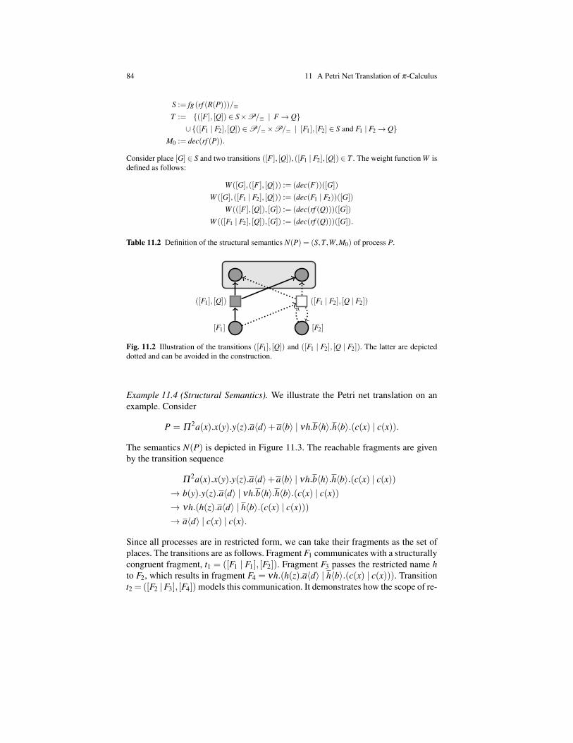
84 11 A Petri Net Translation of π-Calculus
S := fg(rf (R(P)))/≡T := ([F ], [Q]) ∈ S×P/≡ | F → Q∪([F1 | F2], [Q]) ∈P/≡×P/≡ | [F1], [F2] ∈ S and F1 | F2→ Q
M0 := dec(rf (P)).
Consider place [G] ∈ S and two transitions ([F ], [Q]),([F1 | F2], [Q]) ∈ T . The weight function W isdefined as follows:
W ([G],([F ], [Q])) := (dec(F))([G])
W ([G],([F1 | F2], [Q])) := (dec(F1 | F2))([G])
W (([F ], [Q]), [G]) := (dec(rf (Q)))([G])
W (([F1 | F2], [Q]), [G]) := (dec(rf (Q)))([G]).
Table 11.2 Definition of the structural semantics N(P) = (S,T,W,M0) of process P.
([F1], [Q]) ([F1 | F2], [Q | F2])
[F1] [F2]
Fig. 11.2 Illustration of the transitions ([F1], [Q]) and ([F1 | F2], [Q | F2]). The latter are depicteddotted and can be avoided in the construction.
Example 11.4 (Structural Semantics). We illustrate the Petri net translation on anexample. Consider
P = Π2a(x).x(y).y(z).a〈d〉+a〈b〉 | νh.b〈h〉.h〈b〉.(c(x) | c(x)).
The semantics N(P) is depicted in Figure 11.3. The reachable fragments are givenby the transition sequence
Π2a(x).x(y).y(z).a〈d〉+a〈b〉 | νh.b〈h〉.h〈b〉.(c(x) | c(x))
→ b(y).y(z).a〈d〉 | νh.b〈h〉.h〈b〉.(c(x) | c(x))→ νh.(h(z).a〈d〉 | h〈b〉.(c(x) | c(x)))→ a〈d〉 | c(x) | c(x).
Since all processes are in restricted form, we can take their fragments as the set ofplaces. The transitions are as follows. Fragment F1 communicates with a structurallycongruent fragment, t1 = ([F1 | F1], [F2]). Fragment F3 passes the restricted name hto F2, which results in fragment F4 = νh.(h(z).a〈d〉 | h〈b〉.(c(x) | c(x))). Transitiont2 =([F2 |F3], [F4]) models this communication. It demonstrates how the scope of re-

11.2 Structural Semantics 85
stricted names influences the Petri net semantics. A pair of processes is representedby a single token on place [F4]. Fragment F4 lets its two processes communicateon the restricted channel h, which yields Q = a〈d〉 | c(x) | c(x) = F6 | F5 | F5. Bydefinition, we get the transition t3 = ([F4], [Q]). The transition shows how fragmentsconsisting of several processes break up when restricted names are forgotten.
[F1]
t1
[F2]
t2 [F3][F4]
t3[F5]
[F6]
t4
2
2
F1 = a(x).x(y).y(z).a〈d〉+a〈b〉 F2 = b(y).y(z).a〈d〉
F3 = νh.b〈h〉.h〈b〉.(c(x) | c(x)) F4 = νh.(h(z).a〈d〉 | h〈b〉.(c(x) | c(x)))F5 = c(x) F6 = a〈d〉
Fig. 11.3 The structural semantics N(P) of process P in Example 11.4. The meaning of transitionsis explained in the text.
The definition of the set of transitions does not take the overall process behaviourinto account. The Petri net may contain transitions that are never enabled. Transitiont4 illustrates this fact. The fragments F1 and F6 communicate to G = d(y).y(z).a〈d〉.This results in t4 = ([F1 | F6], [G]). The transition is never executed since the reactionis not possible in P. Since G is no reachable fragment, (dec(G))([F ]) = 0 for allplaces [F ], so transition t4 has no places in its postset.
The example suggests the following rules of thumb for the structural semantics.
Remark 11.1. Passing restricted names merges fragments. If fragment F passes arestricted name νa to fragment G, this may result in a new fragment νa.(F ′ |G′) andwe have a transition from the places [F ] and [G] to place [νa.(F ′ | G′)]. Transitiont2 in Example 11.4 illustrates the behaviour.
Forgetting restricted names splits fragments. If fragment F forgets the restrictedname a when it evolves to F ′, fragment νa.(F | G) reacts to F ′ | νa.G. This resultsin a transition with [νa.(F | G)] in its preset and [F ′] and [νa.G] in its postset.Transition t3 in Example 11.4 serves as an example.
To ensure that our semantics is a suitable representation of π-Calculus processes,we show that we can retrieve all information about a process and its transitions fromthe semantics. To relate a marking in the Petri net N(P) and a process, we definethe function retrieve : R(N(P))→P/≡. It constructs a process from a marking by

86 11 A Petri Net Translation of π-Calculus
composing (1) the fragments that are marked in parallel (2) as often as required bythe marking. This mimics the construction in the elementary equivalence.
Definition 11.7. Given a process P ∈P , the function retrieve : R(N(P))→P/≡associates with every marking reachable in the structural semantics, M ∈ R(N(P)),a process class [Q] ∈P/≡ as follows:
retrieve(M) := [Π[H]∈supp(M)ΠM([H])H].
The support of M has to be finite to ensure retrieve(M) is a process. This holds sinceevery transition has a finite postset and the initial marking is finite.
The transition systems of P and N(P) are isomorphic. Furthermore, the states inboth transition systems correspond using the retrieve function. This relationship isillustrated in Figure 11.4.
[F1 | F1 | F3] (2 0 1 0 0 0)
[F2 | F3] (0 1 1 0 0 0)
[F4] (0 0 0 1 0 0)
[F5 | F5 | F6] (0 0 0 0 2 1)
iso
Fig. 11.4 Illustration of the transition system isomorphism in Theorem 11.1 on process P fromExample 11.4. The transition system T (P) is depicted to the left, T (N(P)) is depicted to the right.The isomorphism iso : R(P)/≡→ R(N(P)) is represented by dotted arrows.
Theorem 11.1. The transition systems of P ∈P and its structural semantics N(P)are isomorphic. The isomorphism iso : R(P)/≡→ R(N(P)) maps [Q] to dec(rf (Q)).A process is reconstructed from a marking by retrieve(iso([Q])) = [Q].
To prove the theorem one shows that retrieve is the inverse of iso and that iso is anisomorphism between the transition systems, i.e., iso maps the initial process to theinitial marking, iso is bijective, and iso is a strong graph homomorphism. A stronggraph homomorphism requires that [P1]→ [P2] in the transition system of P if andonly if iso([P1])→ iso([P2]) in the transition system of N(P).
The definition of the structural semantics is declarative as it refers to the set ofall reachable fragments and adds transitions where appropriate. In the followingsection, we comment on the implementation.

Chapter 12Structural Stationarity
Abstract Finiteness of N(P)
We proposed a Petri net semantics of π-Calculus that highlights the connectionstructure of processes. Since the π-Calculus is Turing complete but finite Petri netsare not, such a semantics has to yield infinite nets for some processes. The goalof this section is to understand the sources of infinity for the structural semantics.Our interest in finiteness is based on the observation that all automated verificationmethods for Petri nets rely on this constraint. Ultimately this research will lead usto the borderline of decidability for dynamic networks.
For simplicity, call a process P∈P structurally stationary if its Petri net N(P) isfinite. We obtain two alternative characterizations of structural stationarity that referto the parallel composition and to the restriction operator, respectively. The firstcharacterization eases the proof of structural stationarity. The second one revealsthat infinity of the semantics has two sources: unbounded breadth and unboundeddepth. Unbounded breadth is caused by unbounded distribution of restricted names.Unbounded depth is caused by unboundedly long chains of processes connected byrestricted names. In particular, unbounded name and unbounded process creation donot necessarily imply infinite automata-theoretic representations.
12.1 Structural Stationarity and Finiteness
Intuitively, a process is structurally stationary if there is a finite number of fragmentsin the system. Technically, there is a finite set of fragments so that the restricted formof all reachable processes is a parallel composition of those fragments.
Definition 12.1. Process P ∈P is structurally stationary if
∃F1, . . . ,Fn ⊆Pfg : ∀Q ∈ R(P) : ∀F ∈ fg(rf (Q)) : ∃i ∈ [1,n] : F ≡ Fi.
The set of all structurally stationary processes is Pfg<∞.
87

88 12 Structural Stationarity
Lemma 12.1 states the equivalence between finiteness of the structural semanticsand structural stationarity mentioned in the introduction.
Lemma 12.1 (Finiteness). N(P) is finite if and only if P ∈Pfg<∞.
Proof. Finiteness of N(P) = (S,T,W,M0) is equivalent to finiteness of the set ofplaces S = fg(rf (R(P)))/≡. Finiteness of fg(rf (R(P)))/≡ is equivalent to structuralstationarity. ut
To prove structural stationarity is not easy. The difficult part is to come up with asuitable set of fragments F1, . . . ,Fn. The characterization in Section 12.3 reducesthis task to finding a bound on the number of sequential processes in every reachablefragment. To establish completeness of this characterization, i.e., to show structuralstationarity from boundedness, we in fact have to construct a finite set of fragments.The benefit is that we do this construction once when proving Theorem 12.1. Whenthe characterization has been established, we simply apply it whenever we showstructural stationarity. The construction relies on the notion of derivatives.
12.2 Derivatives
The derivatives of a process P can be understood as a finite skeleton for all reachableprocesses. More formally, we show that all reachable processes are created fromderivatives via parallel composition, restriction, and substitution. The correspondingProposition 12.1 is crucial in the proof of Theorem 12.1.
The derivatives are constructed by recursively removing all prefixes from P as ifthey were consumed in communications. If a process identifier K is called, directlyin P or indirectly in one of its defining equations, we also add the derivatives of theprocess defining K.
Definition 12.2. We rely on the auxiliary function der : P → P(P) defined by
der(0) := /0 der(Kbac) := Kbacder(π.P+M) := π.P+M∪der(P)∪der(M) der(P | Q) := der(P)∪der(Q)
der(νa.P) := der(P).
The set of derivatives of P ∈P , denoted by derivatives(P), is the smallest set sothat (1) der(P) ⊆ derivatives(P) and (2) if Kbac ∈ derivatives(P) and K(x) := Qthen also der(Q)⊆ derivatives(P).
There are two differences between the derivatives and the processes obtained bytransitions. Names y that are replaced by received names when an action b(y) isconsumed remain unchanged in the derivatives. Parameters x that are instantiated toa in a call Kbac are not replaced in the derivatives. Both shortcomings are correctedby substitutions applied to the free names in the derivatives. Proposition 12.1 showsthat this yields all reachable processes.

12.3 First Characterization of Structural Stationarity 89
Proposition 12.1. Every process Q ∈ R(P) and every fragment F ∈ fg(rf (Q)) isstructurally congruent to a process ν a.
(Πi∈I Qiσi
)where Qi ∈ derivatives(P) and
σi : fn(Qi)→ fn(P) ∪ a.
The following example provides some intuition to this technical statement.
Example 12.1. Consider P = νb.a〈b〉.b(x) | a(y).Kba,yc with K(a,y) := y〈a〉. Theonly transition sequence is
νb.a〈b〉.b(x) | a(y).Kba,yc → νb.(b(x) | Kba,bc)→ νb.(b(x) | b〈a〉)→ 0.
We compute the set of derivatives:
derivatives(P) = a〈b〉.b(x),b(x),a(y).Kba,yc,Kba,yc,y〈a〉.
The following congruences show that every reachable fragment can be constructedfrom the derivatives as stated in Proposition 12.1:
νb.a〈b〉.b(x)≡ νb.((a〈b〉.b(x))a,b/a,b)a(y).Kba,yc ≡ (a(y).Kba,yc)a/a
νb.(b(x) | Kba,bc)≡ νb.(b(x)b/b | Kba,yca,b/a,y)νb.(b(x) | b〈a〉)≡ νb.(b(x)b/b | y〈a〉b,a/y,a).
In the proof of Theorem 12.1, finiteness of the set of derivatives is important.
Lemma 12.2. The set derivatives(P) is finite for all P ∈P .
12.3 First Characterization of Structural Stationarity
We characterize structural stationarity as mentioned above: structural stationarity isequivalent to boundedness of all reachable fragments in the number of sequentialprocesses. The number of sequential processes in P ∈P is ||P||S ∈ N defined by||0||S := 0 and (with M 6= 0):
||M||S := 1 ||P | Q||S := ||P||S + ||Q||S||Kbac||S := 1 ||νa.P||S := ||P||S.
The function is invariant under structural congruence: P≡ Q implies ||P||S = ||Q||S.Bounding this number means we actually restrict the use of parallel composition. InSection 12.4, we establish a second characterization of structural stationarity, whichrestricts the use of operator ν instead. While the present characterization provides ahandle to proving structural stationarity, the second characterization explains whichprocesses fail to be structurally stationary.
Definition 12.3. A process P ∈P is bounded in the sequential processes if there isa bound on the number of sequential processes in all reachable fragments:

90 12 Structural Stationarity
∃kS ∈ N : ∀Q ∈ R(P) : ∀F ∈ fg(rf (Q)) : ||F ||S ≤ kS.
The set of all processes that are bounded in the sequential processes is PS<∞.
Theorem 12.1. Pfg<∞ = PS<∞.
Proof. ⇒ If P ∈Pfg<∞ then all reachable processes are made up of finitely manyfragments F1, . . . ,Fn. Thus, the number of sequential processes in all reachable frag-ments is bounded by max||Fi||S | 1≤ i≤ n.
⇐ Let P ∈PS<∞ where kS ∈ N is a bound on the number of sequential processesin fragments. We construct a finite set of fragments FG that includes up to structuralcongruence every reachable fragment. The set FG is defined as a union
FG :=kS⋃
i=1
FGi.
The idea is that FGi only contains fragments with i ∈ N sequential processes. Forthe construction of suitable such fragments, we rely on Proposition 12.1. It providesprocesses ν a.(Π i
j=1Q jσ′j) that are sufficient to represent every reachable fragment.
To ensure finiteness, we rename a to distinguished names ui that we define below.We add the restricted form of ν ui.(Π
ij=1Q jσ j) to FGi provided it is a fragment:
FGi :=
rf (ν ui.(Πij=1Q jσ j)) | Q j ∈ derivatives(P), σ j : fn(Q j)→ fn(P)∪ ui,
and rf (ν ui.(Πij=1Q jσ j)) is a fragment
.
We first show that FGi is finite for every i ∈N. The Q j are derivatives of P. This setis finite by Lemma 12.2. The same finiteness means that the maximum maxFN :=max|fn(Q)| | Q ∈ derivatives(P) exists. A parallel composition of i derivativesthus restricts at most i ·maxFN names. Hence, the names ui := u1, . . . ,ui·maxFNare sufficient to reflect all restrictions. There are finitely many substitutions σ j :fn(Q j)→ fn(P)∪ ui between the finite sets fn(Q j) and fn(P)∪ ui. This concludesthe proof of finiteness for FGi. Finiteness of FG follows immediately.
It remains to show that up to structural congruence every reachable fragment F isincluded in FG. With Proposition 12.1, F is structurally congruent with a fragmentrf (ν u|I|.(Πi∈IQiσi)) in FG|I|. The inclusion FG|I| ⊆ FG then follows from
|I|= ||ν u|I|.(Πi∈IQiσi)||S = ||F ||S ≤ kS.
The second equality is due to the invariance of ||− ||S under structural congruence.The inequality is the boundedness assumption. ut
We explain the construction of FG on an example.
Example 12.2 (FG). Reconsider P= νb.a〈b〉.b(x) | a(y).Kba,yc from Example 12.1with K(a,y) := y〈a〉 . The number of sequential processes in all reachable fragmentsis bounded by kS = 2. The set FG is therefore defined as FG = FG1 ∪FG2. The

12.4 Second Characterization of Structural Stationarity 91
maximal number of free names in derivatives is maxFN = 2. Thus, FG1 and FG2contain fragments
rf (νu1,u2.(Qσ)) and rf (νu1, . . . ,u4.(Q1σ1 | Q2σ2)),
where Q ∈ derivatives(P) with σ : fn(Q) → u1,u2,a and Q j ∈ derivatives(P)with σ j : fn(Q j)→ u1, . . . ,u4,a, for j = 1,2. As an example, consider processQ = a〈b〉.b(x) ∈ derivatives(P). Applying the substitutions σ : a,b→ u1,u2,ayields amongst others
νu1.((a〈b〉.b(x))a,u1/a,b) = νu1.a〈u1〉.u1(x) ∈ FG1.
The process is structurally congruent with the reachable fragment νb.a〈b〉.b(x).
Several known subclasses of π-Calculus are immediately shown to be structurallystationary with Theorem 12.1. Furthermore, the proof of Theorem 12.2 underlinesits importance.
12.4 Second Characterization of Structural Stationarity
The characterization of structural stationarity we develop in this section refers tothe restriction operator. We observe that a bounded number of restricted names doesnot imply structural stationarity. In fact, a process with only one restricted namemay not be structurally stationary. Consider νa.Kbac with K(x) := x〈x〉 | Kbxc. Itgenerates processes sending on the restricted channel a. The transition sequence
νa.Kbac → νa.(a〈a〉 | Kbac)→ νa.(a〈a〉 | a〈a〉 | Kbac)→ . . .
forms infinitely many fragments that are pairwise not structurally congruent. In thegraph interpretation in Figure 12.1 there is no bound on the number of verticesconnected with the hyperedge of name a, i.e., the degree of this edge is not bounded.
The degree of a hyperedge is the number of processes that share the name. Toimitate this value at process level, we define ||F || | the maximal number of fragmentsunder a restriction. For example ||νa.Kbac|| | = 1 and ||νa.(a〈a〉 | Kbac)|| | = 2. Toreflect the maximum of the edge degrees, we search for the widest representation FBof a fragment F . Widest means that ||FB|| | is maximal in the congruence class.
Kbac a → Kbac a
a〈a〉
→ Kbac a
a〈a〉
a〈a〉 → . . .
Fig. 12.1 Transition sequence illustrating unbounded breadth

92 12 Structural Stationarity
Definition 12.4. The maximal number of fragments under a restriction is definedinductively by ||M|| | := 1, ||Kbac|| | := 1, and
||νa.(F1 | . . . | Fn)|| | := maxn, ||F1|| | , . . . , ||Fn|| | .
The breadth of fragment F is ||F ||B := max||G|| | | G ≡ F. Process P ∈P isbounded in breadth, denoted by P∈PB<∞, if the breadth of all reachable fragmentsis bounded:
∃kB ∈ N : ∀Q ∈ R(P) : ∀F ∈ fg(rf (Q)) : ||F ||B ≤ kB.
By definition, the breadth is invariant under structural congruence: F ≡ G implies||F ||B = ||G||B. As it refers to all fragments in the congruence class, the notion is hardto grasp. We provide an example that illustrates the definition.
Example 12.3 (Breadth). Consider νa.Lbacwith L(x) := νb.(x〈b〉 | x〈b〉 | Lbxc). Theonly transition sequence is
νa.Lbac → νa.(νa1.(a〈a1〉 | a〈a1〉) | Lbac)→ νa.(νa1.(a〈a1〉 | a〈a1〉) | νa2.(a〈a2〉 | a〈a2〉) | Lbac)→ . . .
After n ∈ N transitions we have the following fragment FD ≡ FB:
FD = νa.(Π ni=1νai.(a〈ai〉 | a〈ai〉) | Lbac)
FB = νa1.(. . .(νan.(νa.(Π ni=1(a〈ai〉 | a〈ai〉) | Lbac))) . . .).
We have ||FD|| | = n+1 and ||FB|| | = 2n+1. In FB the number of fragments undera restriction is maximal in the congruence class of FD ≡ FB. So after n transitionswe have ||FD||B = ||FB||B = ||FB|| | = 2n+1. There is no bound on the breadth of thereachable fragments, νa.Lbac /∈PB<∞.
aKbac
→ ab〈a〉
bKbbc
→ ab〈a〉
bc〈b〉
cKbcc
→ . . .
Fig. 12.2 Transition sequence illustrating unbounded depth
Bounding the breadth of fragments is not sufficient to show structural stationarity.Consider νa.Kbac with K(x) := νb.(b〈x〉 | Kbbc). The process generates infinitelymany fragments that are pairwise not structurally congruent but have breadth two:
νa.Kbac → νa.(νb.(b〈a〉 | Kbbc))→ νa.(νb.(b〈a〉 | νc.(c〈b〉 | Kbcc)))→ . . .
In the graphs in Figure 12.2, the length of the simple paths is not bounded. Recallthat a path is simple if it does not repeat hyperedges. At process level, we mimicthis length by the nesting of restrictions ||F ||ν . In the example, ||νa.Kbac||ν = 1 and

12.4 Second Characterization of Structural Stationarity 93
||νa.(νb.(b〈a〉 |Kbbc))||ν = 2. To ensure the restrictions contribute to a simple path,we consider the flattest representation FD of F where ||FD||ν is minimal.
Definition 12.5. The nesting of restrictions ||F ||ν is defined by ||M||ν := 0 whereM 6= 0, ||Kbac||ν := 0, and
||νa.(F1 | . . . | Fn)||ν := 1+max||F1||ν , . . . , ||Fn||ν.
With this auxiliary function, the depth of F is ||F ||D :=min||G||ν | G≡F. ProcessP ∈P is bounded in depth, P ∈PD<∞, if
∃kD ∈ N : ∀Q ∈ R(P) : ∀F ∈ fg(rf (Q)) : ||F ||D ≤ kD.
Also the depth of fragments is invariant under structural congruence, ||F ||D = ||G||Dfor fragments F ≡ G. We continue with process νa.Lbac from Example 12.3.
Example 12.4 (Depth). After n ∈ N transitions we have FD ≡ FB:
FD = νa.(Π ni=1νai.(a〈ai〉 | a〈ai〉) | Lbac)
FB = νa1.(. . .(νan.(νa.(Π ni=1(a〈ai〉 | a〈ai〉) | Lbac))) . . .).
We have ||FD||ν = 2 and ||FB||ν = n+ 1.The nesting in FD is minimal in the class.Thus, ||FB||D = ||FD||D = ||FD||ν = 2. So the depth of all fragments reachable fromνa.Lbac is bounded by two, νa.Lbac ∈PD<∞.
There are at most ||F || | fragments under a restriction. The nesting of restrictions isat most ||F ||ν . Thus, the number of sequential processes in F is bounded as follows.
Lemma 12.3. ||F ||S ≤ ||F ||||F ||ν| .
Proof. We proceed by an induction on the structure of fragments. In the base case,we have F = M 6= 0 and F = Kbac. The desired inequality holds with
||F ||S = 1 = 10 = ||F ||||F ||ν| .
For the induction step, assume ||Fi||S ≤ ||Fi||||Fi||ν| for all Fi with 1 ≤ i ≤ n. We then
have for F = νa.(F1 | . . . | Fn):
||F ||S Def. ||F ||S = Σ
ni=1||Fi||S
Hypothesis ≤ Σni=1||Fi||||Fi||ν
|
Def. max ≤ Σni=1max||Fi|| | | 1≤ i≤ nmax||Fi||ν | 1≤i≤n.
Abbreviate max| := max||Fi|| | | 1≤ i≤ n and maxν := max||Fi||ν | 1≤ i≤ n.With this, the above term equals

94 12 Structural Stationarity
n ·maxmaxν
|
Def. max ≤ maxn,max| ·maxn,max|maxν
= maxn,max|1+maxν
Def. ||F ||ν and ||F || | = ||F ||||F ||ν| .
ut
Together, boundedness in breadth and in depth yield structural stationarity — themain result in this section. While the previous proof of structural stationarity fromboundedness in the sequential processes was direct and cumbersome, Theorem 12.1now yields an elegant proof of Theorem 12.2: a process is structurally stationary ifand only if it is bounded in breadth and bounded in depth.
Theorem 12.2. Pfg<∞ = PB<∞∩PD<∞.
Proof. ⇒ If the process is structurally stationary, there is a finite set of fragmentsF1, . . . ,Fn so that every reachable fragment is structurally congruent with an Fi.Then the maxima max||Fi||D | 1 ≤ i ≤ n and max||Fi||B | 1 ≤ i ≤ n exist andbound the depth and the breadth of all reachable fragments.
⇐ If we assume boundedness in breadth and depth there are kB and kD so thatfor all Q ∈ R(P) and all F ∈ fg(rf (Q)) we have ||F ||B ≤ kB and ||F ||D ≤ kD. Weshow that kkD
B is a bound on the number of sequential processes. Consider Q ∈ R(P)and F ∈ fg(rf (Q)). We determine the flattest representation FD ≡ F that satisfies||FD||ν = min||G||ν | G≡ F= ||F ||D. We now have
||F ||S ||− ||S invariant under ≡ = ||FD||S
Lemma 12.3 ≤ ||FD||||FD||ν|
||FD|| | ≤ max||G|| | | G≡ F= ||F ||B ≤ ||F ||||FD||νB
Observation ||FD||ν = ||F ||D = ||F ||||F ||DB
kB and kD bounds on breadth and depth ≤ kkDB .
This proves P is bounded in the number of sequential processes. With Theorem 12.1,P is structurally stationary. ut
Theorem 12.2 helps disproving structural stationarity. A process is not structurallystationary if and only if it is not bounded in breadth or not bounded in depth. Thus,there are two sources of infinity for the structural semantics.
For processes of bounded depth but unbounded breadth, termination can beshown to be decidable by an instantiation of the WSTS framework. Processes ofbounded breadth but unbounded depth are Turing complete. This follows from anencoding of counter machines that we present in the following chapter.
Chapter 13Undecidability Results
Abstract Undecidability results for π-Calculus
There are several machine models with the ability to perform arithmetic operationson data variables, which are known to be Turing complete. For the undecidabilityproofs in this chapter, we use a model introduced by Minsky. Although Minskycalled his formalism a program machine that operates on registers, the model isnowadays well-known under the name of (2-)counter machines acting on countervariables. We exploit Turing completeness of counter machines to show Turingcompleteness for processes of bounded breadth. As a consequence, we obtain un-decidability of structural stationarity, boundedness in depth, and boundedness inbreadth. We then change the encoding to establish undecidability of reachability forprocesses of depth one.
13.1 Counter Machines
A counter machine has two counters c1 and c2 that store arbitrarily large naturalnumbers and a finite sequence of labelled instructions l : op. There are two kinds ofoperations op. The first increments a counter, say c1, by one and then jumps to theinstruction labelled by l′:
c1 := c1 +1 goto l′ (13.1)
The second operation has the form
if c1 = 0 then goto l′; else c1 := c1−1; goto l′′; (13.2)
95
96 13 Undecidability Results
It checks counter c1 for being zero and—if this is the case—jumps to the instructionlabelled by l′. If the value of c1 is positive, the counter is decremented by one andthe machine jumps to l′′.
Definition 13.1. A counter machine is a triple CM = (c1,c2, instr) where c1,c2 arecounters and instr = l0 : op0; . . . , ln : opn; ln+1 : halt is a finite sequence of the labelledinstructions defined above. The sequence ends with operation halt to terminate theexecution.
To define the operational semantics of a counter machine CM, we define the notionof a configuration. A configuration of CM is a triple cf = (v1,v2, l), where vi ∈ Nis the current value of counter ci with i = 1,2 and l ∈ l0, . . . , ln+1 is the label ofthe operation to be executed next. A run of CM is a finite or infinite sequence ofconfigurations
cf 0→ cf 1→ cf 2→ . . .
subject to the following constraints. Initially, the counter values are zero and l0 is thenext instruction to be executed, cf 0 = (0,0, l0). For every transition cf i→ cf i+1 withcf i = (v1,v2, l) the values of the counters and the instruction are changed accordingto the current operation op with l : op. In case op is an increment operation for thefirst counter as defined in (13.1), we have cf i+1 = (v1 +1,v2, l′). This means valuev1 is incremented, v2 is not changed, and the current label is changed to l′. Thedecrement operation on c1 in (13.2) depends on whether v1 = 0 holds. In this case,we jump to l′ without modifying the counter values, cf i+1 = (v1,v2, l′). If the contentof c1 is positive, we decrement it and jump to l′′, which yields cf i+1 = (v1−1,v2, l′′).Action halt does not yield a transition.
We say CM terminates if all its runs are finite. A configuration cf = (v1,v2, l) isreachable in CM if there is a run cf 0→ . . .→ cf k = cf for some k∈N. Since countermachines are Turing complete, termination and reachability are undecidable.
Theorem 13.1 (Minsky 1967). Counter machines are Turing complete. Hence, fora counter machine CM it is undecidable whether (1) CM terminates and (2) whethera given configuration cf is reachable in CM.
13.2 From Counter Machines to Bounded Breadth
The idea is to encode counters by lists. To fix the terminology, a list consists oflist elements, namely several list items and one list end. The number of list itemsrepresents the value of the counter. Every list item and the list end has three channelsto communicate on—reflecting the three operations on counters. Channel i is usedfor increment operations. Thus, a communication on i appends a list item to the list.Communications on channel d decrement the counter value. A message on t is atest for zero. We first explain the behaviour of a list item. To keep the definitionshort, we abbreviate i,d, t by c. Similarly, the channels i′,d′, t ′ of the following list

13.2 From Counter Machines to Bounded Breadth 97
element are abbreviated by c′. Since we are only interested in the channels, we omitparameters x in send and receive actions i〈x〉 and i(x):
LI(c, c′) := i.i′.LIbc, c′c+d.(d′.LIbc, c′c+ t ′.LEbcc
).
An increment operation received on channel i is passed to the following list elementwith the send action i′. As a list item stands for a positive counter value, the test forzero fails. A list item does not communicate on channel t. If a list item receives adecrement, it contacts the following list element. Since it is unknown whether thisis a list item LI or a list end LE, the current list item tries to communicate on bothchannels d′ and t ′. If the next element is a list item, it answers the decrement call. Alist end receives the t ′ message and, as a reaction, terminates. Now the current listitem is the last element and therefore calls the defining equation LEbcc.
A list end answers a test for zero and terminates. As it represents value zero, itdoes not listen on the decrement channel. If the list end receives an increment, itcreates new control channels c′ = i′,d′, t ′ and a new list end process LEbc′c. Theformer list end becomes a list item by calling the defining equation LIbc, c′c:
LE(c) := t + i.ν c′.(LIbc, c′c | LEbc′c).
Every instruction l : op of the counter machine translates into a process identifierKl whose defining process is determined by the operation op. For the incrementoperation (13.1) on counter c1, we get
Kl(c1, c2) := i1.Kl′bc1, c2c.
The parameters c1 = i1,d1, t1 and c2 = i2,d2, t2 are the control channels of the liststhat represent the counters c1 and c2, respectively.
The encoding of the decrement operation in (13.2) contains a subtlety. If the testfor zero is successful, we delete the list end of counter c1 and have to create a newone. This yields
Kl(c1, c2) := t1.ν c′1.(Kl′bc′1, c2c | LEbc′1c
)+d1.Kl′′bc1, c2c.
The instruction l : halt is translated into Kl(c1, c2) := halt. The send action will behelpful later to prove undecidability of boundedness in breadth.
To sum up, the counter machine CM is translated into the process
P(CM) := ν c1.ν c2.(LEbc1c | LEbc2c | Kl0bc1, c2c)
Example 13.1. Configuration (2,0, l) of a counter machine is represented by
ν c1.[ν c′1.
(LIbc1, c′1c | ν c′′1 .(LIbc′1, c′′1c | LEbc′′1c)
)| ν c2.
(LEbc2c | Klbc1, c2c
)].
There are two list items in the list for c1 to represent counter value two. Similarly,the list of counter c2 consists of a single list end. The label of the current instructioncan be deduced from the process identifier Kl.

98 13 Undecidability Results
Example 13.1 suggests a tight relationship between the configurations reachable ina counter machine CM and the processes reachable in its encoding P(CM). We shallonly need that the encoding preserves termination.
Proposition 13.1. CM terminates if and only if P(CM) terminates.
The process representation of a counter machine is bounded in breadth by two.We exploit this observation in the following section to establish undecidability ofboundedness in depth and breadth.
Lemma 13.1. For every counter machine CM we have P(CM) ∈PB<∞.
With proper synchronization mechanisms, the construction can be modified so thatthe steps of the counter machine coincide with step sequences of the correspondingprocess.
Remark 13.1. Processes of bounded breadth PB<∞ are Turing complete.
13.3 Undecidability of Structural Stationarity
To show undecidability of structural stationarity for processes of bounded breadth,we reduce the termination problem for counter machines. This works as terminatingprocesses are structurally stationary or, in contraposition, non-structurally stationaryprocesses do not terminate. For structurally stationary processes we can use thestructural semantics to decide termination.
Proposition 13.2 (Undecidability of Structural Stationarity). For P∈PB<∞ it isundecidable whether P ∈Pfg<∞ holds.
input : CM a counter machine
begincompute P(CM)
if ¬isStructurallyStationary(P(CM)) thenreturn CM does not terminate
elsecompute N(P(CM))
return terminates(N(P(CM)))
end
Fig. 13.1 Proof of undecidability of structural stationarity. The procedure checks whether acounter machine terminates, assuming isStructurallyStationary(−) decides structural stationarityfor PB<∞. Procedure terminates(−) decides termination for Petri nets.
13.3 Undecidability of Structural Stationarity 99
Proof. Assume structural stationarity is decidable for processes of bounded breadthusing the procedure isStructurallyStationary(−). Figure 13.1 gives an algorithm thatthen decides termination of a given counter machine CM as follows. We computethe process P(CM) ∈PB<∞. If the process is not structurally stationary it does notterminate. By Proposition 13.1, CM does not terminate.
If P(CM) is a structurally stationary process, the structural semantics N(P(CM))is a finite Petri net by Lemma 12.1. For finite Petri nets, termination is decidable.Moreover, the net terminates if and only if the counter machine does:
CM terminates Proposition 13.1 ⇔ P(CM) terminates Theorem 11.1 ⇔ N(P(CM)) terminates.
Since termination of counter machines is undecidable, the assumption that structuralstationarity is decidable for PB<∞ has to be false. ut
For a process of bounded breadth the condition of structural stationarity is equivalentto boundedness in depth according to Theorem 12.2. Since structural stationarity isundecidable, boundedness in depth is.
Corollary 13.1 (Undecidability of Boundedness in Depth). Consider P ∈PB<∞.It is undecidable whether P ∈PD<∞ holds.
To conclude the section, we reduce termination of CM to deciding boundedness inbreadth. We again exploit the fact that our process representation P(CM) of countermachines is bounded in breadth. The idea of the reduction is to compose P(CM) inparallel with
halt.νa.KB=∞bac.
When this process consumes halt it generates fragments of unbounded breadth.Consequently, CM terminates if and only if the parallel composition is not boundedin breadth.
Lemma 13.2 (Undecidability of Boundedness in Breadth). For a process P ∈Pit is undecidable whether P ∈PB<∞ holds.
Proof. Consider the counter machine CM and the process
P(CM) | halt.νa.KB=∞bac
with KB=∞(a) := a〈a〉 | KB=∞bac. The counter machine terminates if and only if itreaches its halt operation. This is the case if and only if process P(CM) sends halt.Since P(CM) is bounded in breadth, reachability of halt is equivalent to unbound-edness in breadth for P(CM) | halt.νa.KB=∞bac. ut

100 13 Undecidability Results
13.4 Undecidability of Reachability in Depth 1
To establish undecidability of reachability for processes of depth one, we reduce thecorresponding problem for counter machines. Since the resulting processes have tobe bounded in depth, we can no longer represent counter values by lists. Instead,we use a different encoding that reflects counter values by parallel composition. Forexample, c1 = 3 yields a | a | a.
The problem with this representation is that parallel compositions, very similarto Petri nets, cannot faithfully model a test for zero:
l : if c1 = 0 then goto l′; else c1 := c1−1 goto l′′;
To overcome this problem, we use the following trick. We implement a test for zeroby a nondeterministic choice between a decrement and a test operation. If the testwas done incorrectly (we branch to l′ although c1 > 0), we reach an error process.From an error process we can never get back to a counter machine configuration.Technically, an error process leaves garbage νa.(a | a | a) that cannot be removed.We turn to the construction.
We attach the processes a to a so-called process bunch PBba, ic1 ,dc1 , tc1c. To setup this link, we simply restrict the name a. For counter value c1 = 3, this gives
νa.(PBba, ic1 ,dc1 , tc1c | a | a | a).
Due to the restriction, the process bunch PBba, ic1 ,dc1 , tc1c has exclusive access toits processes a. It offers three operations to modify their numbers: ic1 , dc1 , and tc1 .Communications on ic1 stand for increment and create a new process a. Similarly,a message on dc1 decrements the process number by consuming a process a. Atest for zero on tc1 creates a new and empty process bunch for counter c1. Theold process bunch terminates. A term νa.(a | a | a) without process bunch is thegarbage that was mentioned above. The names ic1 , dc1 , and tc1 are free. Their indexc1 indicates that the process bunch models counter c1. We abbreviate the parameterlist by cx = icx ,dcx , tcx for x ∈ 1,2 and define
PB(a, cx) := ix.(PBba, cxc | a) + dx.a.PBba, cxc + tx.νb.PBbb, cxc.
The computational strength in this construction is in the process bunch deletion. Thischanges the linkage of an arbitrary number of processes a with a single transition.
The translation of the labelled instructions is similar to the one in Section 13.2.An increment operation l : c1 := c1 +1 goto l′ yields a process identifier
Kl(c1, c2) := ic1 .Kl′bc1, c2c.
The test for zero discussed above yields a nondeterministic choice
Kl(c1, c2) := tc1 .Kl′bc1, c2c + dc1 .Kl′′bc1, c2c.

13.4 Undecidability of Reachability in Depth 1 101
A process bunch may accept a decrement although it is empty. In this case, thesystem deadlocks and reachability is preserved. A halt l : halt translates intoKl(c1, c2) := halt. The full translation of counter machine CM is the process
P1(CM) := νa.PBba, c1c | νb.PBbb, c2c | Kl0bc1, c2c. (13.3)
Example 13.2. Consider counter machine CM = (c1,c2, instr) with
instr :l0 : c1 := c1 +1 goto l1;l1 : if c1 = 0 then goto l1; else c1 := c1−1 goto l2;l2 : halt.
The machine sets c1 to one, the following check for zero fails, c1 is decremented,and the machine stops. The associated process P1(CM) has the form in (13.3) withthe following defining equations:
Kl0(c1, c2) := ic1 .Kl1bc1, c2cKl1(c1, c2) := tc1 .Kl1bc1, c2c + dc1 .Kl2bc1, c2cKl2(c1, c2) := halt.
The reachable states of CM can be computed from the reachable processes ofP1(CM). More precisely, the counter machine CM reaches the state (v1,v2, l) if andonly if its encoding reaches the process
νa.(PBba, c1c |Π v1a) | νb.(PBbb, c2c |Π v2b) | Klbc1, c2c.
Combined with the observation that P1(CM) is always bounded in depth by one, wearrive at the desired undecidability.
Theorem 13.2. Consider two processes P,Q ∈PD<∞ where the depth is boundedby one. The problem whether [Q] ∈ R(P)/≡ is undecidable.
Theorem 13.2 implies undecidability of reachability for processes of bounded depth.Termination, in turn, can be shown to be decidable for PD<∞. Since terminationis undecidable for counter machines, the above encoding P1(CM) cannot preservetermination. Example 13.2 gives a counter machine CM that terminates but whoseprocess representation P1(CM) has an infinite run.
Since reachability is decidable for Petri nets, we conclude that there is noreachability-preserving translation into Petri nets for any class of processes thatsubsumes those of depth one.