Embed Size (px)
Citation preview

Oasys Concrete Code Reference

13 Fitzroy Street
London
W1T 4BQ
Telephone: +44 (0) 20 7755 3302
Facsimile: +44 (0) 20 7755 3720
Central Square
Forth Street
Newcastle Upon Tyne
NE1 3PL
Telephone: +44 (0) 191 238 7559
Facsimile: +44 (0) 191 238 7555
e-mail: [email protected]
Website: oasys-software.com
Oasys
© Oasys 1985 – 2017
All rights reserved. No parts of this work may be reproduced in any form or by any means - graphic, electronic,
or mechanical, including photocopying, recording, taping, or information storage and retrieval systems - without
the written permission of the publisher.
Products that are referred to in this document may be either trademarks and/or registered trademarks of the
respective owners. The publisher and the author make no claim to these trademarks.
While every precaution has been taken in the preparation of this document, the publisher and the author
assume no responsibility for errors or omissions, or for damages resulting from the use of information
contained in this document or from the use of programs and source code that may accompany it. In no event
shall the publisher and the author be liable for any loss of profit or any other commercial damage caused or
alleged to have been caused directly or indirectly by this document.

Oasys
© Oasys Ltd 2016
Contents
Notation 6
Design Codes 7
Concrete material models 8
Units 8
Parabola-rectangle 10
EC2 Confined 11
Rectangle 11
Bilinear 13
FIB 13
Popovics 14
Mander & Mander confined curve 16
BS8110-2 tension curve 17
TR59 18
Interpolated 19
Concrete properties 20
ACI 21
AS 22
BS 5400 23
BS 8110 25
CSA A23.3 / CSA S6 26
EN 1992 27
HK CP 29
IRS Bridge 33
Rebar material models 36
Rebar material models for different codes 36
Elastic-plastic 37
Elastic-hardening 37
Progressive yield 39
Park 40
Linear 41
Creep 42
EN 1992-1-1 42
Oasys
© Oasys Ltd 2016
AS 3600 – 2009 43
Hong Kong Code of Practice 44
ACI 209.2R-18 46
IRC : 112-2011 47
IS 456 : 2000 48
IRS Concrete Bridge Code : 1997 48
Oasys
© Oasys Ltd 2016
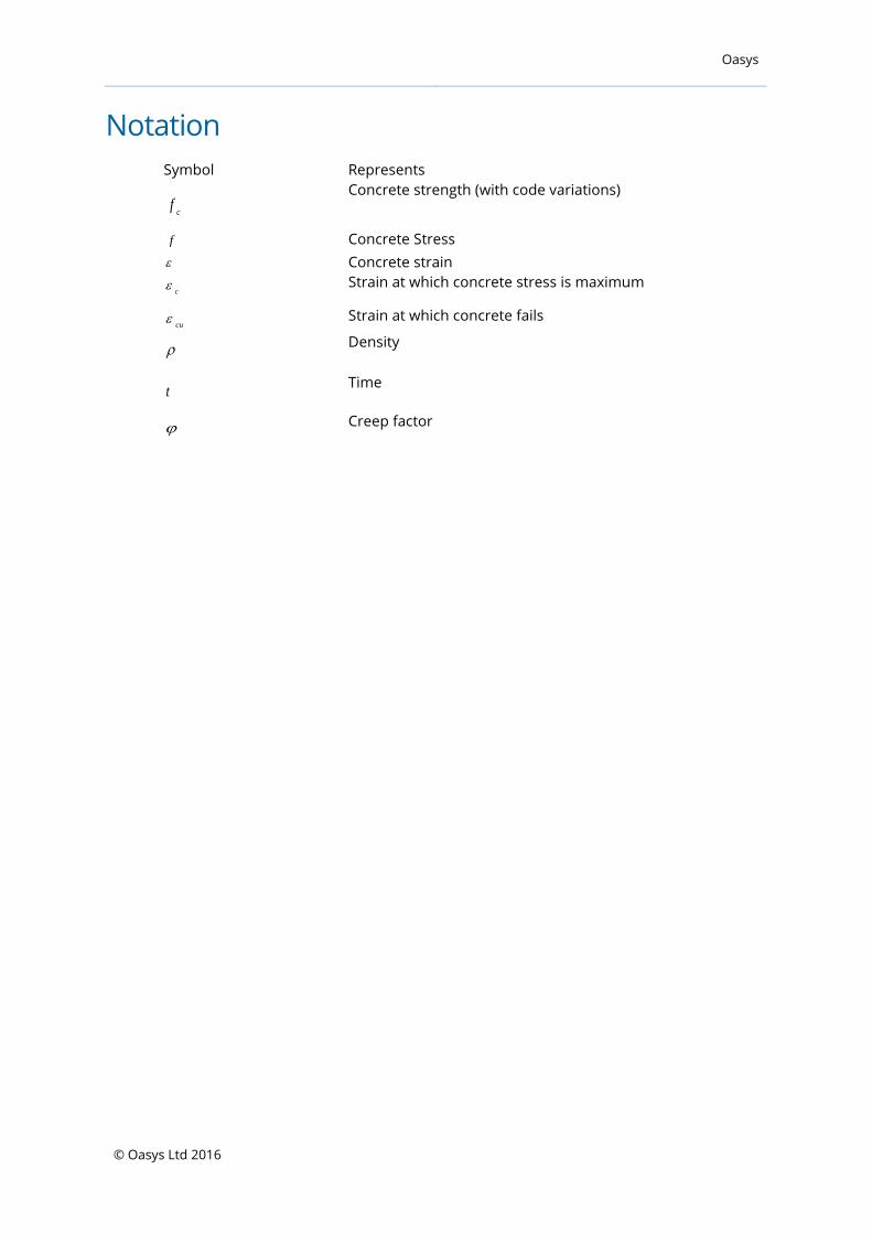
Notation
Symbol Represents
cf
Concrete strength (with code variations)
f
Concrete Stress
Concrete strain
c
Strain at which concrete stress is maximum
cu
Strain at which concrete fails
Density
t Time
Creep factor

Oasys
© Oasys Ltd 2016
Design Codes
The following design codes are supported to varying degrees in the Oasys software
products.
Code Title Country Date Other
versions
ACI318 Building Code Requirements for
Structural Concrete (ACI318-14)
USA 2014 2011, 2008,
2005, 2002
ACI318M Building Code Requirements for
Structural Concrete (ACI318M-14)
(metric version)
USA 2014 2011, 2008,
2005, 2002
AS3600 Australian Standard Concrete
Structures 2009
Australia 2009 2001
BS5400-4 Steel, concrete and composite bridges
– Code of practice for design of
concrete bridges
UK 1990 IAN70/06
BS8110-1 Structural Use of Concrete Part 1.
Code of practice for design and
construction (Incorporating
Amendments Nos. 1, 2 and 3)
UK 2005 1997, 1985
BS EN 1992-1-1 Eurocode 2-1 UK 2004 PD6687:2006
BS EN 1992-2 Eurocode 2-2 UK 2005
CAN CSA A23.3 Design of Concrete Structures Canada 2014 2004
CAN CSA S6 Canadian Highway Bridge Design Code Canada 2014
CYS EN 1992-1-1 Eurocode 2-1-1 Cyprus 2004
DIN EN 1992-1-1 Eurocode 2-1-1 Germany 2004
DIN EN 1992-2 Eurocode 2-2 Germany 2010
DS/EN 1992-1-1 Eurocode 2-1-1 Denmark 2004
DS/EN 1992-2 Eurocode 2-2 Denmark 2005
EN1992-1-1 Eurocode 2: Design of concrete
structures – Part 1-1: General rules
and rules for buildings
2004
EN 1992-2 Eurocode 2: Design of concrete
structures. Concrete bridges - Design
and detailing rules
2005
Hong Kong Code
of Practice
Code of Practice for the Structural Use
of Concrete
Hong Kong 2013 2004 (AMD
2007), 2004,
1987
Oasys
© Oasys Ltd 2016
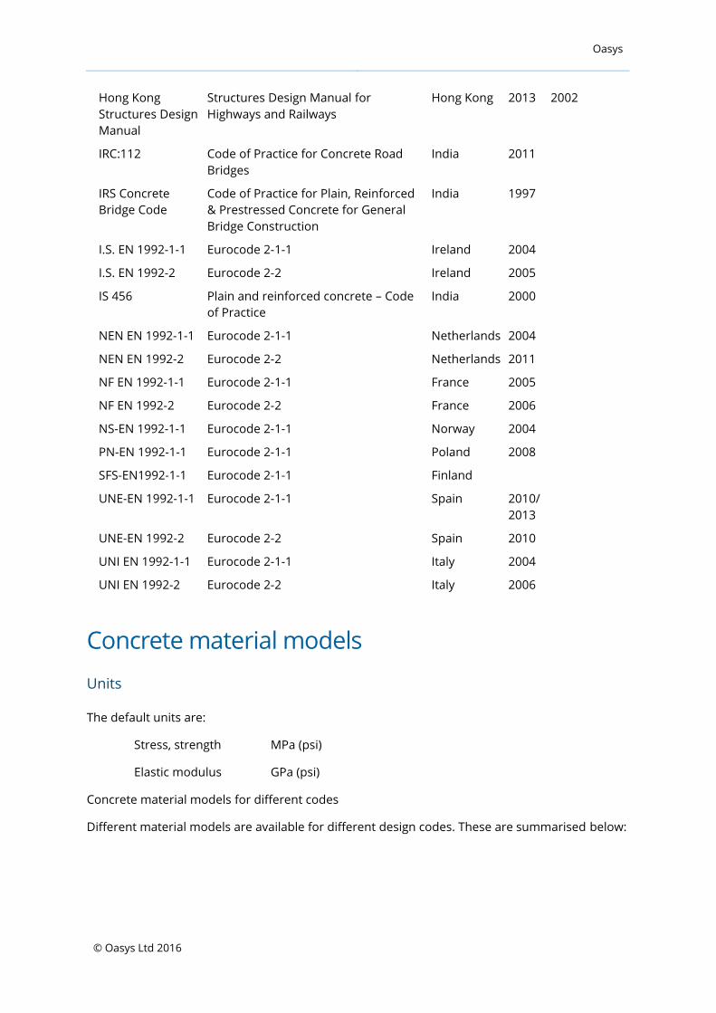
Hong Kong
Structures Design
Manual
Structures Design Manual for
Highways and Railways
Hong Kong 2013 2002
IRC:112 Code of Practice for Concrete Road
Bridges
India 2011
IRS Concrete
Bridge Code
Code of Practice for Plain, Reinforced
& Prestressed Concrete for General
Bridge Construction
India 1997
I.S. EN 1992-1-1 Eurocode 2-1-1 Ireland 2004
I.S. EN 1992-2 Eurocode 2-2 Ireland 2005
IS 456 Plain and reinforced concrete – Code
of Practice
India 2000
NEN EN 1992-1-1 Eurocode 2-1-1 Netherlands 2004
NEN EN 1992-2 Eurocode 2-2 Netherlands 2011
NF EN 1992-1-1 Eurocode 2-1-1 France 2005
NF EN 1992-2 Eurocode 2-2 France 2006
NS-EN 1992-1-1 Eurocode 2-1-1 Norway 2004
PN-EN 1992-1-1 Eurocode 2-1-1 Poland 2008
SFS-EN1992-1-1 Eurocode 2-1-1 Finland
UNE-EN 1992-1-1 Eurocode 2-1-1 Spain 2010/
2013
UNE-EN 1992-2 Eurocode 2-2 Spain 2010
UNI EN 1992-1-1 Eurocode 2-1-1 Italy 2004
UNI EN 1992-2 Eurocode 2-2 Italy 2006
Concrete material models
Units
The default units are:
Stress, strength MPa (psi)
Elastic modulus GPa (psi)
Concrete material models for different codes
Different material models are available for different design codes. These are summarised below:

Oasys
© Oasys Ltd 2016
AC
I 3
18
AS
36
00
BS
54
00
BS
81
10
CS
A A
23
.3
CS
A S
6
EN
19
92
HK
CP
HK
SD
M
IRC
:11
2
IRS
Bri
dg
e
IS 4
56
Compression
Parabola-
rectangle ● ● ● ● ● ● ● ● ● ● ● ●
Rectangle ● ● ● ● ● ● ● ● ●
Bilinear ● ●
Linear ● ● ● ● ● ● ● ● ● ● ● ●
FIB ● ● ● ● ●
Popovics ● ● ● ●
EC2
Confined ● ●
AISC 360
filled tube ●
Explicit ● ● ● ● ● ● ● ● ● ● ● ●
Tension
No-tension ● ● ● ● ● ● ● ● ● ● ● ●
Linear ● ● ● ● ● ● ● ● ●
Interpolate
d ● ● ● ● ● ●
BS8110 - 2 ● ● ●
Oasys
© Oasys Ltd 2016
TR 59 ● ● ●
PD 6687 ●
Explicit ● ● ● ● ● ● ● ● ● ● ● ●
Explicit
envelope ● ● ● ● ● ● ● ● ● ● ● ●
inferred from rectangular block
PD 6687 variant of EN 1992 only
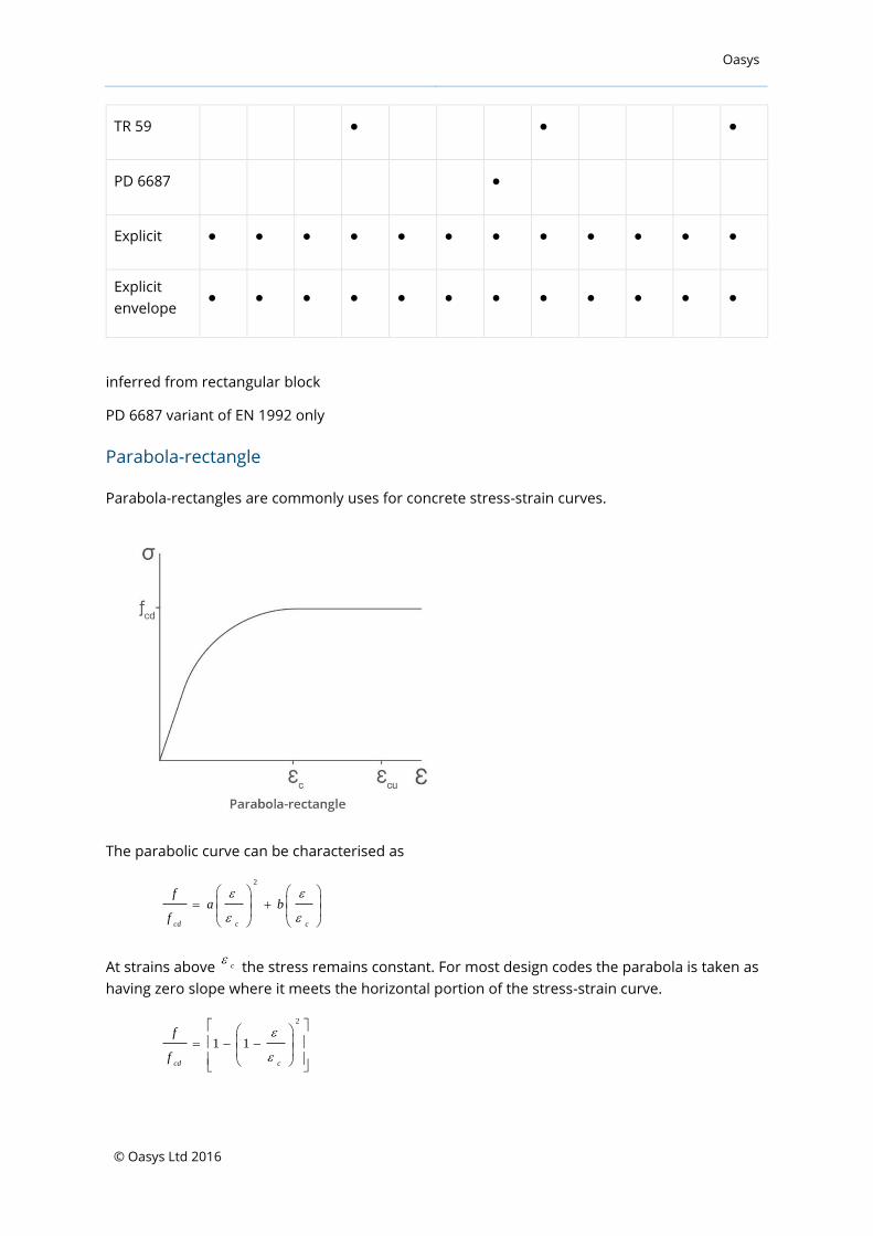
Parabola-rectangle
Parabola-rectangles are commonly uses for concrete stress-strain curves.
The parabolic curve can be characterised as
cccd
baf
f
2
At strains above c
the stress remains constant. For most design codes the parabola is taken as
having zero slope where it meets the horizontal portion of the stress-strain curve.
2
11
ccdf
f

Oasys
© Oasys Ltd 2016
The Hong Kong Code of Practice (supported by the Hong Kong Institution of Engineers) interpret
the curve so that the initial slope is the elastic modulus (meaning that the parabola is not
tangent to the horizontal portion of the curve).
cscscdE
E
E
E
f
f
2
1
where the secant modulus is
c
cd
s
fE
In Eurocode the parabola is modified
n
ccdf
f
11
and
2n cf
≤ 50MPa
4
100904.234.1c
fn c
f> 50MPa
EC2 Confined
The EC2 confined model is a variant on the parabola-rectangle. In this case the confining stress increases the compressive strength and the plateau and failure strains.
ccc
ccc
cc
fff
ffff
05.05.2125.1
05.051
,
ccuccu
cccccc
f
ff
2.0,
2
,,
Rectangle
The rectangular stress block has zero stress up to a strain of c
(controlled by
) and then a
constant stress of cdf
.

Oasys
© Oasys Ltd 2016
α β
ACI 318 1 0.85 - 0.05(fc - 30)/7 [0.65:0.85]
AS3600 2001 1 0.85 - 0.07(fc - 28) [0.65:0.85]
AS3600 2009 1 1.05 - 0.007fc [0.67:0.85]
BS5400 0.6/0.67 1
BS8110 1 0.9
CSA A23.3 1 max(0.67, 0.97 - 0.0025 fc)
CSA S6 1 max(0.67, 0.97 - 0.0025 fc)
EN 1992 1 fc ≤ 50MPa
1 - (fc - 50)/200 fc> 50MPa
0.8 fc ≤ 50MPa
0.8 - (fc - 50)/400 fc > 50MPa
HK CP > 2004 1 0.9
HK CP 2007 > 1
0.9 fc ≤ 45MPa
0.8 fc ≤ 70MPa
0.72 fc ≤ 100MPa

Oasys
© Oasys Ltd 2016
HK SDM 0.6/0.67 1
IRC:112 1 fc≤ 60MPa
1 - (fc - 60)/250 fc> 60MPa
0.8 fc≤ 60MPa
0.8 - (fc - 60)/500 fc> 60MPa
IRS Bridge 0.6/0.67 1
IS 456 0.8 0.84
Bilinear
The bilinear curve is linear to the point
cdcf,
and then constant to failure.
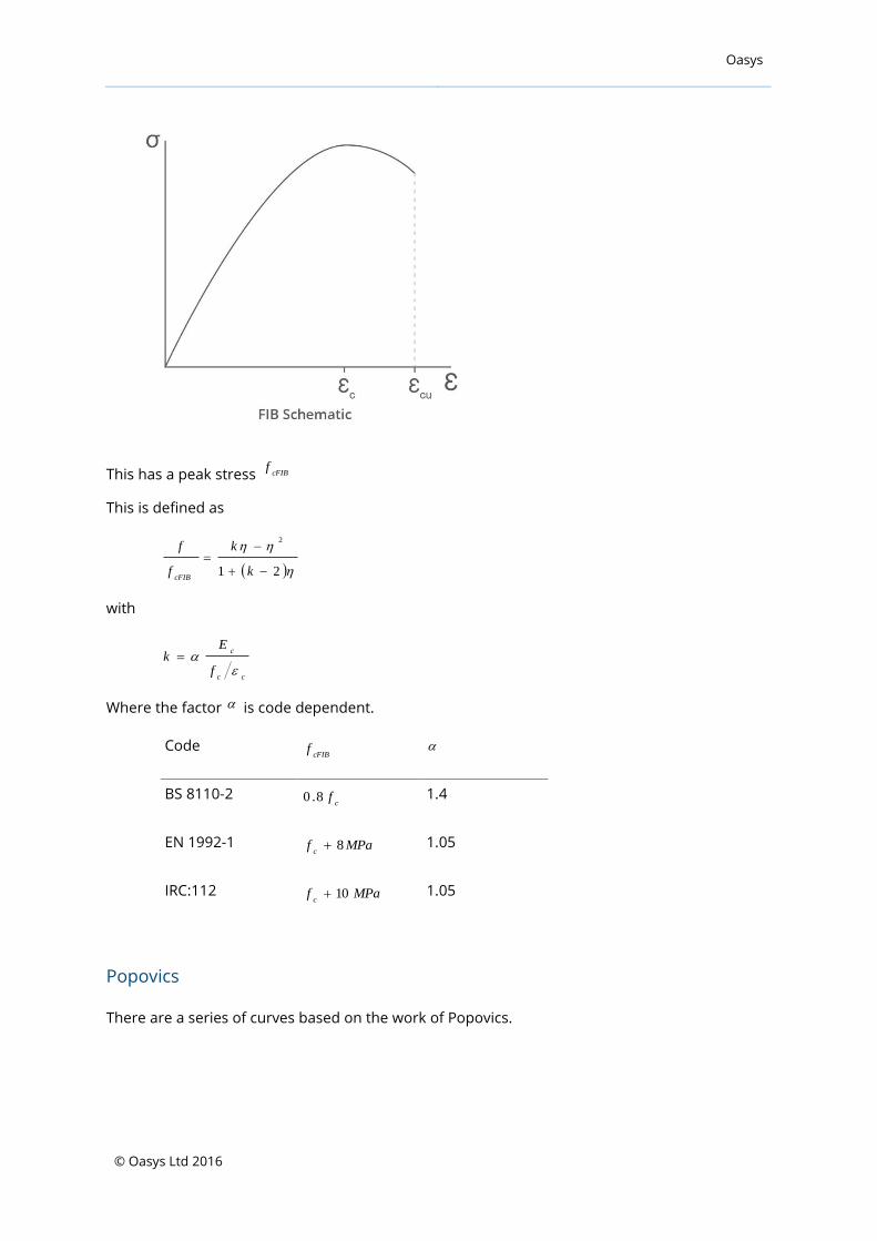
FIB
The FIB model code defines a schematic stress-strain curve. This is used in BS 8110-2, EN1992-1
and IRC:112.
Oasys
© Oasys Ltd 2016
This has a peak stress cFIBf
This is defined as
21
2
k
k
f
f
cFIB
with
cc
c
f
Ek
Where the factor is code dependent.
Code cFIB
f
BS 8110-2 c
f8.0
1.4
EN 1992-1 MPafc
8
1.05
IRC:112 MPafc
10
1.05
Popovics
There are a series of curves based on the work of Popovics.

Oasys
© Oasys Ltd 2016
These have been adjusted and are based on the Thorenfeldt base curve.
In the Canadian offshore code (CAN/CSA S474-04) this is characterised by
nk
cn
nk
f
f
13
with (in MPa)
c
cf
k10
6.03
178.0
cf
n
1
n
n
E
f
c
c
c
1
6267.0
11
cfk
The peak strain is referred to elsewhere as pop
.
cpop
All the concrete models require a strength value and a pair of strains: the strain at peak stress or
transition strain and the failure strain.

Oasys
© Oasys Ltd 2016
Mander & Mander confined curve
The Mander1 curve is available for both strength and serviceability analysis and the Mander
confined curve for strength analysis.
For unconfined concrete, the peak of the stress-strain curve occurs at a stress equal to the
unconfined cylinder strength cf
and strain c
generally taken to be 0.002. Curve constants are
calculated from
ccfE
sec
and
secEE
Er
Then for strains c 20
the stress can be calculated from:
rc
r
rf
1
where
c
1 Mander J, Priestly M, and Park R. Theoretical stress-strain model for confined concrete. Journal
of Structural Engineering, 114(8), pp1804-1826, 1988.

Oasys
© Oasys Ltd 2016
The curve falls linearly from c2
2eco to the ‘spalling’ strain cu
. The spalling strain can be taken
as 0.005-0.006.
To generate the confined curve the confined strength ccf
, must first be calculated. This will
depend on the level of confinement that can be achieved by the reinforcement. The maximum
strain ccu ,
also needs to be estimated. This is an iterative calculation, limited by hoop rupture,
with possible values ranging from 0.01 to 0.06. An estimate of the strain could be made from EC2
formula (3.27) above with an upper limit of 0.01.
The peak strain for the confined curve cc ,
is given by:
151
,
,
c
cc
ccc
f
f
Curve constants are calculated from
ccccfE
,,sec
and
secEE
Er
as before.
E is the tangent modulus of the unconfined curve, given above.
Then for strains ccu ,0
the stress can be calculated from:
rcc
r
rf
1,
where
cc ,
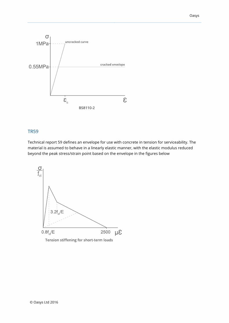
BS8110-2 tension curve
BS8110-2 define a tension curve for serviceability
Oasys
© Oasys Ltd 2016
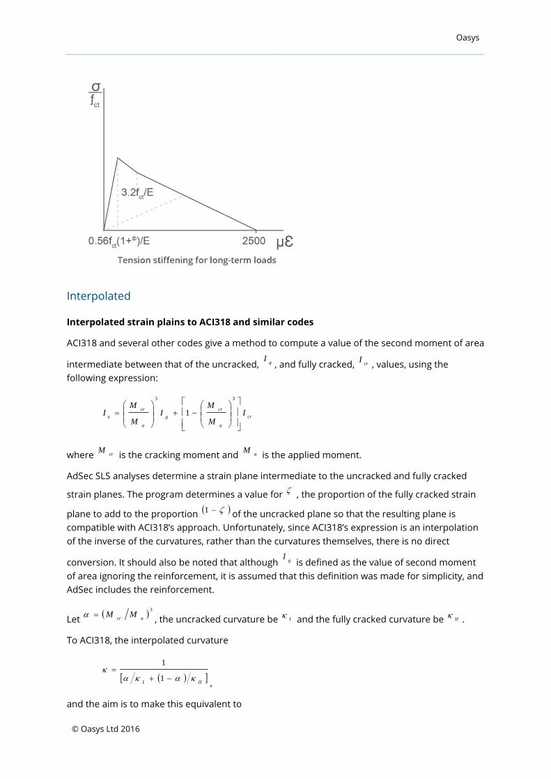
TR59
Technical report 59 defines an envelope for use with concrete in tension for serviceability. The
material is assumed to behave in a linearly elastic manner, with the elastic modulus reduced
beyond the peak stress/strain point based on the envelope in the figures below
Oasys
© Oasys Ltd 2016
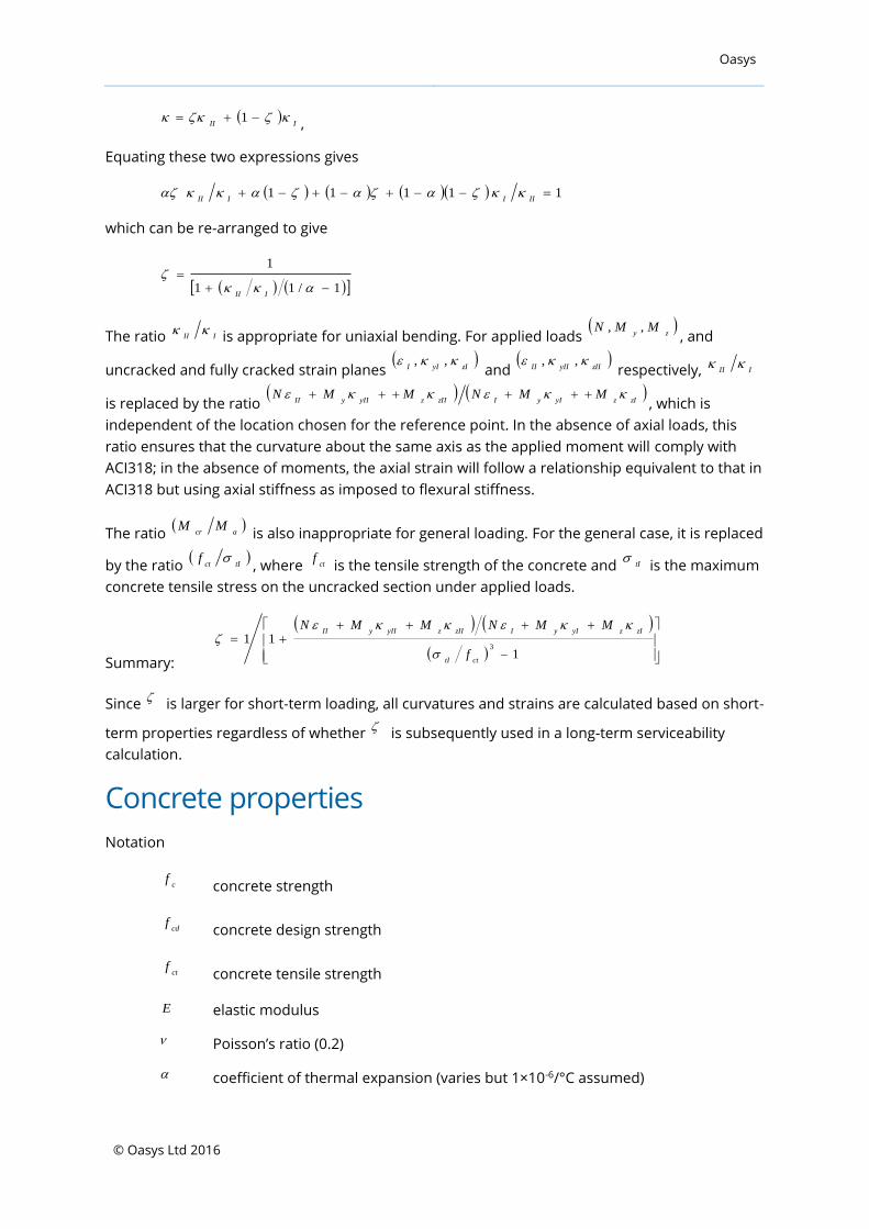
Interpolated
Interpolated strain plains to ACI318 and similar codes
ACI318 and several other codes give a method to compute a value of the second moment of area
intermediate between that of the uncracked, gI
, and fully cracked, crI
, values, using the
following expression:
cr
a
cr
g
a
cr
eI
M
MI
M
MI
33
1
where crM
is the cracking moment and aM
is the applied moment.
AdSec SLS analyses determine a strain plane intermediate to the uncracked and fully cracked
strain planes. The program determines a value for
, the proportion of the fully cracked strain
plane to add to the proportion 1
of the uncracked plane so that the resulting plane is
compatible with ACI318’s approach. Unfortunately, since ACI318’s expression is an interpolation
of the inverse of the curvatures, rather than the curvatures themselves, there is no direct
conversion. It should also be noted that although gI
is defined as the value of second moment
of area ignoring the reinforcement, it is assumed that this definition was made for simplicity, and
AdSec includes the reinforcement.
Let
3
acrMM
, the uncracked curvature be I
and the fully cracked curvature be II
.
To ACI318, the interpolated curvature
III
1
1
,
and the aim is to make this equivalent to
Oasys
© Oasys Ltd 2016
III 1 ,
Equating these two expressions gives
11111
IIIIII
which can be re-arranged to give
1/11
1
III
The ratio III is appropriate for uniaxial bending. For applied loads
zy
MMN ,,, and
uncracked and fully cracked strain planes
zIyII ,,
and
zIIyIIII ,,
respectively, III
is replaced by the ratio
zIzyIyIzIIzyIIyIIMMNMMN
, which is
independent of the location chosen for the reference point. In the absence of axial loads, this
ratio ensures that the curvature about the same axis as the applied moment will comply with
ACI318; in the absence of moments, the axial strain will follow a relationship equivalent to that in
ACI318 but using axial stiffness as imposed to flexural stiffness.
The ratio
acrMM
is also inappropriate for general loading. For the general case, it is replaced
by the ratio
tIctf
, where ctf
is the tensile strength of the concrete and tI
is the maximum
concrete tensile stress on the uncracked section under applied loads.
Summary:
1
113
cttI
zIzyIyIzIIzyIIyII
f
MMNMMN
Since
is larger for short-term loading, all curvatures and strains are calculated based on short-
term properties regardless of whether
is subsequently used in a long-term serviceability
calculation.
Concrete properties
Notation
cf
concrete strength
cdf
concrete design strength
ctf
concrete tensile strength
E elastic modulus
Poisson’s ratio (0.2)
coefficient of thermal expansion (varies but 1×10⁻⁶/°C assumed)
Oasys
© Oasys Ltd 2016
cu
strain at failure (ULS)
ax
compressive strain at failure (ULS)
plas
strain at which maximum stress is reached (ULS)
max
assumed maximum strain (SLS)
peak
strain corresponding to (first) peak stress (SLS)
pop
strain corresponding to peak stress in Popovics curve (SLS)
u
1
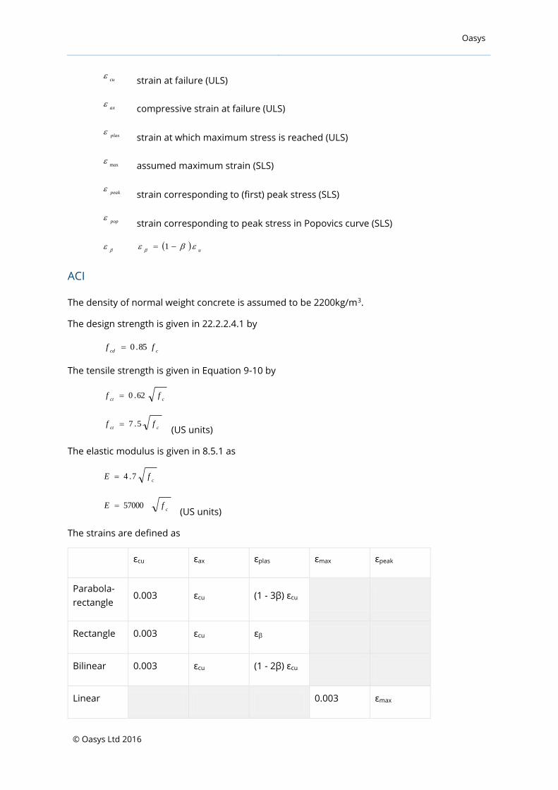
ACI
The density of normal weight concrete is assumed to be 2200kg/m3.
The design strength is given in 22.2.2.4.1 by
ccdff 85.0
The tensile strength is given in Equation 9-10 by
cctff 62.0
cctff 5.7
(US units)
The elastic modulus is given in 8.5.1 as
cfE 7.4
cfE 57000
(US units)
The strains are defined as
εcu εax εplas εmax εpeak
Parabola-
rectangle 0.003 εcu (1 - 3β) εcu
Rectangle 0.003 εcu εβ
Bilinear 0.003 εcu (1 - 2β) εcu
Linear 0.003 εmax
Oasys
© Oasys Ltd 2016
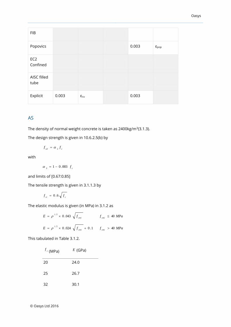
FIB
Popovics 0.003 εpop
EC2
Confined
AISC filled
tube
Explicit 0.003 εcu 0.003
AS
The density of normal weight concrete is taken as 2400kg/m3(3.1.3).
The design strength is given in 10.6.2.5(b) by
ccdff
2
with
cf003.01
2
and limits of [0.67:0.85]
The tensile strength is given in 3.1.1.3 by
cctff 6.0
The elastic modulus is given (in MPa) in 3.1.2 as
MPaffE
cmicmi40043.0
5.1
MPaffE
cmicmi401.0024.0
5.1
This tabulated in Table 3.1.2.
cf
(MPa) E (GPa)
20 24.0
25 26.7
32 30.1

Oasys
© Oasys Ltd 2016
40 32.8
50 34.8
65 37.4
80 39.6
100 42.2
The strains are defined as
εcu εax εplas εmax εpeak
Parabola-
rectangle
Rectangle 0.003 0.0025 εβ 0.003 εβ
Bilinear
Linear 0.003 εmax
FIB
Popovics εmax εpop
EC2
Confined
AISC filled
tube
Explicit 0.003 0.0025 0.003
BS 5400
The density of normal weight concrete is given in Appendix B as 2300kg/m3.
The design strength is given in Figure 6.1 by
ccdff 6.0

Oasys
© Oasys Ltd 2016
The tensile strength is given in 6.3.4.2 as
cctff 36.0
but A.2.2 implies a value of 1MPa should be used at the position of tensile reinforcement.
The elastic modulus tabulated in 4.3.2.1 Table 3
cf
(MPa) E (GPa)
20 25.0
25 26.0
32 28.0
40 31.0
50 34.0
60 36.0
The strains are defined as
εcu εax εplas εmax εpeak
Parabola-
rectangle 0.0035 εcu εRP
Rectangle
Bilinear
Linear 0.0035 εmax
FIB
Popovics
EC2
Confined
AISC filled
tube

Oasys
© Oasys Ltd 2016
Explicit 0.0035 εcu 0.0035
c
RP
f4
104.2
BS 8110
The density of normal weight concrete is given in section 7.2 of BS 8110-2 as 2400kg/m3.
The design strength is given in Figure 3.3 by
ccdff 67.0
The tensile strength is given in 4.3.8.4 as
cctff 36.0
but Figure 3.1 in BS 8110-2 implies a value of 1MPa should be used at the position of tensile
reinforcement.
The elastic modulus is given in Equation 17
cfE 2.020
The strains are defined as
εcu εax εplas εmax εpeak
Parabola-
rectangle εu εcu εRP 0.0035* εRP
Rectangle εu εcu εβ
Bilinear
Linear εu εmax
FIB εu 0.0022
Popovics
EC2
Confined

Oasys
© Oasys Ltd 2016
AISC filled
tube
Explicit εu εcu εu
50
60001.00035.0
600035.0
c
c
uf
MPaf
c
RP
f4
104.2
CSA A23.3 / CSA S6
The density of normal weight concrete is assumed to be 2300 kg/m3; see 8.6.2.2 (A23.3) and
8.4.1.7 (S6).
The design strength is given in 10.1.7 by
cccdfff 0015.085.0,67.0max
The tensile strength is given in Equation 8.3 (A23.3) and 8.4.1.8.1 in (S6)
cctff 6.0
(for CSA A23.3)
cctff 4.0
(for CSA S6)
For normal weight concrete the modulus is given in A23.3 Equation 8.2.
cfE 5.4
and in CSA S6 8.4.1.7
9.60.3
cfE
The strains are defined as
εcu εax εplas εmax εpeak
Parabola-
rectangle 0.0035 εcu (1 - 3β) εu
Rectangle 0.0035 εcu εβ

Oasys
© Oasys Ltd 2016
Bilinear 0.0035 εcu (1 - 2β) εu
Linear 0.0035 εmax
FIB
Popovics 0.0035 εpop
EC2
Confined
AISC filled
tube
Explicit 0.0035 εcu 0.0035
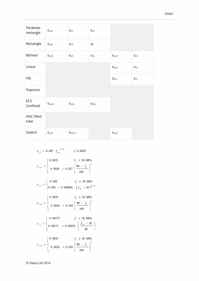
EN 1992
The density of normal weight concrete is specified in 11.3.2 as 2200 kg/m3.
The design strength is given in 3.1.6 by
ccccdff
For the rectangular stress block this is modified to
ccccdff
MPaf
c50
cccccdfff 250125.1
MPaf
c50
The tensile strength is given in Table 3.1 as
3
2
3.0cct
ff
MPafc
50
1081ln12.2
cctff
MPaf
c50
The modulus is defined in Table 3.1
3.0
10
822
cf
E
The strains are defined as
εcu εax εplas εmax εpeak
Oasys
© Oasys Ltd 2016
Parabola-
rectangle εcu2 εc2 εc2
Rectangle εcu3 εc3 εβ
Bilinear εcu3 εc3 εc3 εcu3 εc3
Linear εcu2 εc2
FIB εcu1 εc1
Popovics
EC2
Confined εcu2,c εc2,c εc2,c
AISC filled
tube
Explicit εcu2 εcu2 ? εcu2
0028.0007.0
31.0
1
cmcf
4
1
100
90027.00028.0
500035.0
c
c
cuf
MPaf
53.02
50000085.0002.0
50002.0
ck
c
c
f
MPaf
4
2
100
90035.00026.0
500035.0
c
c
cuf
MPaf
40
5000055.000175.0
5000175.0
3 ck
c
cf
MPaf
4
3
100
90035.00026.0
500035.0
c
c
cuf
MPaf

Oasys
© Oasys Ltd 2016
HK CP
The density of normal weight concrete is assumed to be 2400kg/m3.
The design strength is given in Figure 6.1 by
ccdff 67.0
The tensile strength is given in 12.3.8.4 as
cctff 36.0
but 7.3.6 implies a value of 1MPa should be used at the position of tensile reinforcement.
The elastic modulus is defined in 3.1.5
21.346.3 fcE
The strains are defined as
εcu εax εplas εmax εpeak
Parabola-
rectangle εu εcu εRP
Rectangle εu εcu εβ
Bilinear
Linear εu εu
FIB εu 0.0022
Popovics
EC2
Confined
AISC filled
tube
Explicit εu εcu εu
MPaff
ccu606000006.00035.0

Oasys
© Oasys Ltd 2016
d
c
RP
c
d
E
f
GPaf
E
34.1
21.346.3
HK SDM
The density of normal weight concrete is assumed to be 2400kg/m3.
The design strength is given in 5.3.2.1(b) of BS 5400-4 by
ccdff 6.0
The tensile strength is given in 6.3.4.2 as
cctff 36.0
but from BS5400 a value of 1MPa should be used at the position of tensile reinforcement.
The elastic modulus is tabulated in Table 21
cf
(MPa) E (GPa)
20 18.9
25 20.2
32 21.7
40 24.0
45 26.0
50 27.4
55 28.8
60 30.2
The strains are defined as
εcu εax εplas εmax εpeak
Parabola-
rectangle 0.0035 εcu εRP

Oasys
© Oasys Ltd 2016
Rectangle
Bilinear
Linear 0.0035 εmax
FIB
Popovics
EC2
Confined
AISC filled
tube
Explicit 0.0035 εcu 0.0035
c
RP
f4
104.2
IRC 112
The density of normal eight concrete is assume to be 2200kg/m3.
The design strength is given in 6.4.2.8
ccdff 67.0
In A2.9(2) the strength is modified for the rectangular stress block to
ccdff 67.0
MPaf
c60
cccdfff 25024.167.0
MPaf
c60
The tensile strength is given in by A2.2(2) by
3
2
259.0cct
ff
MPafc
60
5.12101ln27.2
cctff
MPaf
c60
The elastic modulus is given in A2.3, equation A2-5
3.0
5.12
1022
cf
E

Oasys
© Oasys Ltd 2016
The strains are defined as
εcu εax εplas εmax εpeak
Parabola-
rectangle εcu2 εc2 εc2 εcu2 εc2
Rectangle εcu3 εc3 εβ
Bilinear εcu3 εc3 εc3 εcu3 εc3
Linear εcu2 εc2
FIB εcu1 εc1
Popovics
EC2
Confined εcu2,c εc2,c εc2,c
AISC filled
tube
Explicit εcu2 εcu2 ? εcu2
0028.01000653.0
31.0
1
ccf
4
1
100
8.090027.00028.0
600035.0
c
c
cuf
MPaf
53.02
508.0000085.0002.0
60002.0
ck
c
c
f
MPaf
4
2
100
8.090035.00026.0
600035.0
c
c
cuf
MPaf
40
508.000055.000175.0
6000175.0
3 ck
c
cf
MPaf

Oasys
© Oasys Ltd 2016
4
3
100
8.090035.00026.0
500035.0
c
c
cuf
MPaf
IRS Bridge
The density is assumed to be 2300kg/m3.
The design strength is given in 15.4.2.1(b) by
ccdff 6.0
The tensile strength is given in 16.4.4.3 as
cctff 37.0
The elastic modulus is tabulated in 5.2.2.1
cf
(MPa) E (GPa)
20 25.0
25 26.0
32 28.0
40 31.0
50 34.0
60 36.0
The strains are defined as
εcu εax εplas εmax εpeak
Parabola-
rectangle 0.0035 εcu εRP
Rectangle
Bilinear
Oasys
© Oasys Ltd 2016
Linear 0.0035 εmax
FIB
Popovics
EC2
Confined
AISC filled
tube
Explicit 0.0035 εcu 0.0035
c
RP
f4
104.2
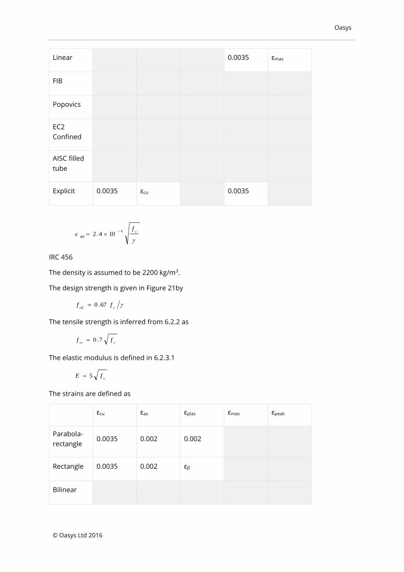
IRC 456
The density is assumed to be 2200 kg/m3.
The design strength is given in Figure 21by
ccdff 67.0
The tensile strength is inferred from 6.2.2 as
cctff 7.0
The elastic modulus is defined in 6.2.3.1
cfE 5
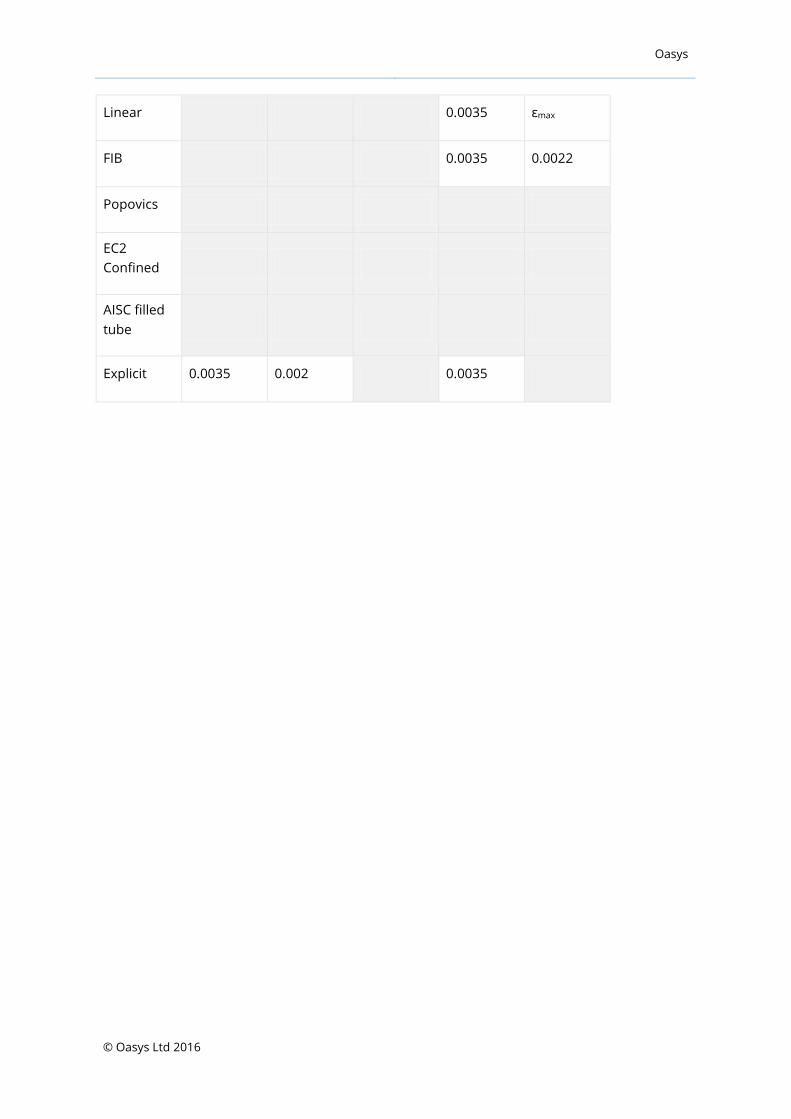
The strains are defined as
εcu εax εplas εmax εpeak
Parabola-
rectangle 0.0035 0.002 0.002
Rectangle 0.0035 0.002 εβ
Bilinear
Oasys
© Oasys Ltd 2016
Linear 0.0035 εmax
FIB 0.0035 0.0022
Popovics
EC2
Confined
AISC filled
tube
Explicit 0.0035 0.002 0.0035
Oasys
© Oasys Ltd 2016
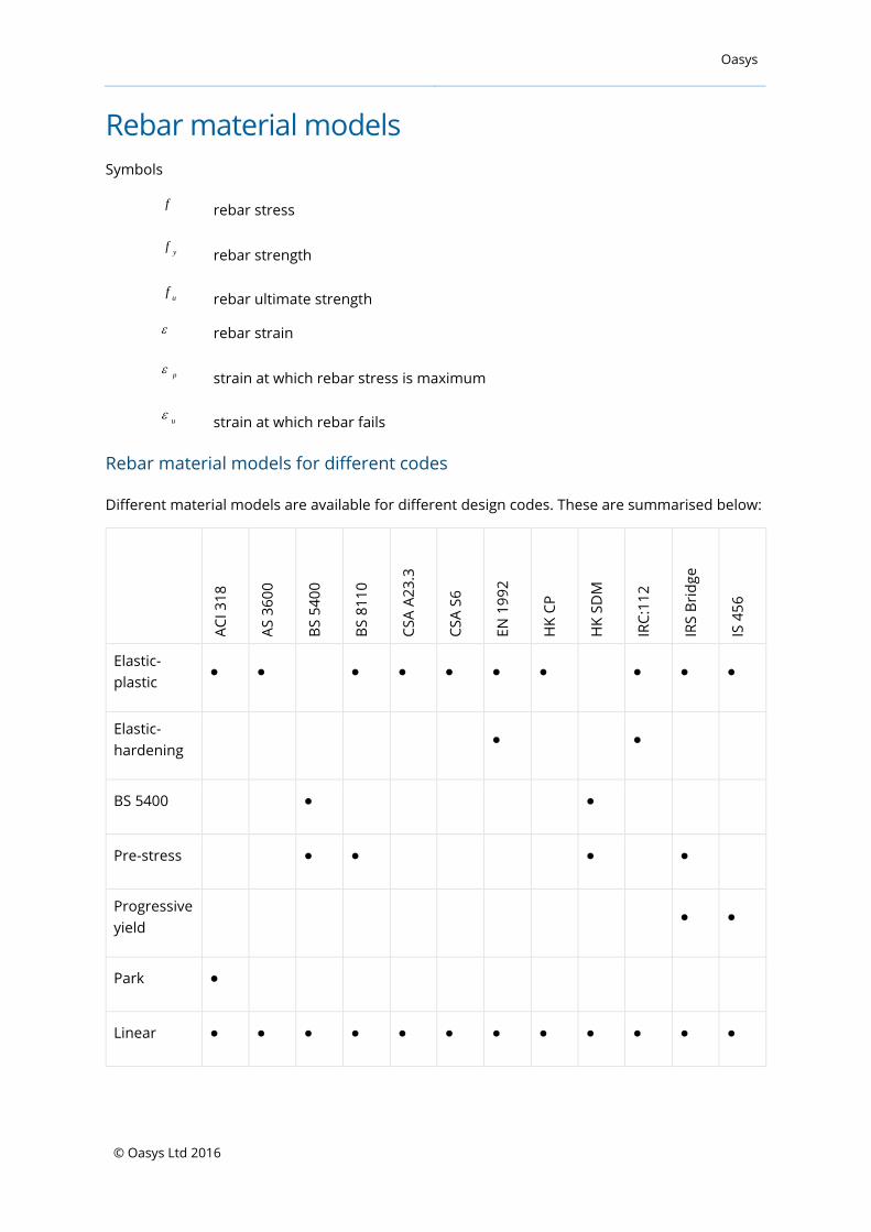
Rebar material models
Symbols
f rebar stress
yf
rebar strength
uf
rebar ultimate strength
rebar strain
p
strain at which rebar stress is maximum
u
strain at which rebar fails
Rebar material models for different codes
Different material models are available for different design codes. These are summarised below:
AC
I 3
18
AS
36
00
BS
54
00
BS
81
10
CS
A A
23
.3
CS
A S
6
EN
19
92
HK
CP
HK
SD
M
IRC
:11
2
IRS
Bri
dg
e
IS 4
56
Elastic-
plastic ● ● ● ● ● ● ● ● ● ●
Elastic-
hardening ● ●
BS 5400 ● ●
Pre-stress ● ● ● ●
Progressive
yield ● ●
Park ●
Linear ● ● ● ● ● ● ● ● ● ● ● ●

Oasys
© Oasys Ltd 2016
No-
compressio
n
● ● ● ● ● ● ● ● ● ● ● ●
ASTM
strand ● ●
Explicit ● ● ● ● ● ● ● ● ● ● ● ●
Elastic-plastic
The initial slope is defined by the elastic modulus, E . Post-yield the stress remains constant until
the failure strain, u
, is reached.
For some codes (CAN/CSA) the initial slope is reduced to E
.
Elastic-hardening
The initial slope is defined by the elastic modulus, E , after yield the hardening modulus hE
governs as stress rises from
ydyf,
to
uuf,
. For EN 1992 the hardening modulus is defined
in terms of a hardening coefficient k and the final point is
ydukkf,
where the failure strain is
reduced to ud
(typically uk9.0
).
The relationship between hardening modulus and hardening coefficient is:

Oasys
© Oasys Ltd 2016
Ef
fkE
yuk
y
h
1
1
y
yukh
f
EfEk
The material fails at ud
where ukud
. This is defined in Eurocode and related codes.
BS 5400
In tension the initial slope is defined by the elastic modulus, E , until the stress reaches ydefk
.
The slope then reduces until the material is fully plastic, ydf
, at Ef
ydoff
. Post-yield the

Oasys
© Oasys Ltd 2016
stress remains constant until the failure strain, u
, is reached. For BS5400 8.0
ek
and
002.0off
.
In compression the initial slope is defined by the elastic modulus, E , until the stress reaches
ydefk
or a strain of off
. It then follows the slope of the tension curve post-yield and when the
strain reaches off
the stress remain constant until failure
Pre-stress
The initial slope is defined by the elastic modulus, E , until the stress reaches ydefk
. The slope
then reduces until the material is fully plastic, ydf
, at Ef
ydoff
. Post-yield the stress
remains constant until the failure strain, u
, is reached. For BS8110 and related codes 8.0
ek
and 005.0
off
.
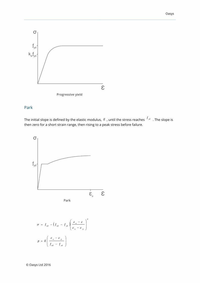
Progressive yield
The initial slope is defined by the elastic modulus, E , until the stress reaches ydefk
. The slope
then reduces in a series of steps until the material is fully plastic, after which the stress remain
constant. The points defining the progressive yield are code dependent.
Oasys
© Oasys Ltd 2016
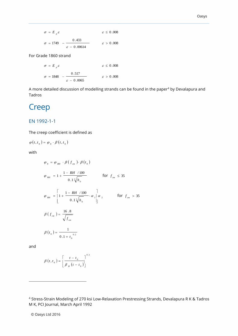
Park
The initial slope is defined by the elastic modulus, E , until the stress reaches ydf
. The slope is
then zero for a short strain range, then rising to a peak stress before failure.
p
pu
u
ydududfff
ydud
pu
ffEp

Oasys
© Oasys Ltd 2016
Linear
The initial slope is defined by the elastic modulus, E , until the failure strain is reached.
No-compression
This is a linear model when in tension which has no compressive strength.
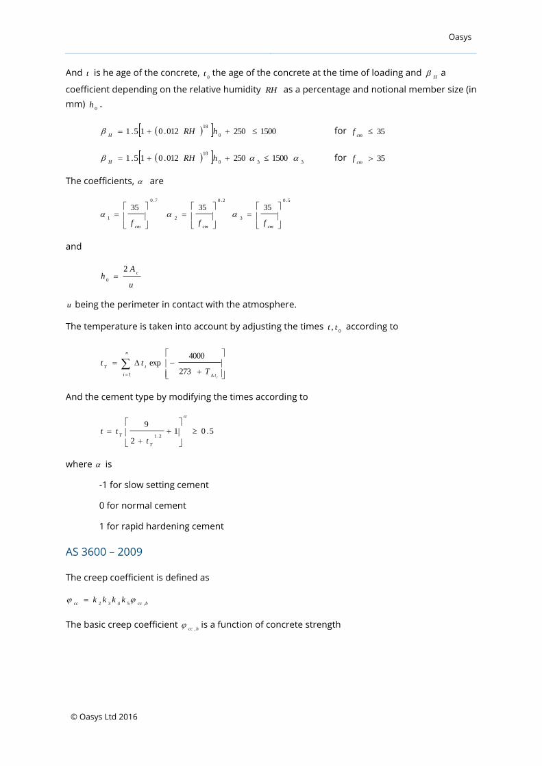
ASTM strand
The ASTM A 416 defines a stress-strain curve doe seven-wire strands. This has an initial linear
relationship up to a strain of 0.008 with progressive yield till failure.
The stress strain curves are defined for specific strengths.
For Grade 2502 (1725 MPa) the stress-strain curve is defined as
008.0
006.0
4.01710
008.0197000
For Grade 270 (1860 MPa) the stress-strain curve is defined as
008.0
003.0
517.01848
008.0197000
In the Commentary to the Canadian Bridge 3 code a similar stress-strain relationship is defined.
For Grade 1749 strand
2 Bridge Engineering Handbook, Ed. Wah-Fah Chen, Lian Duan, CRC Press 1999 3 Commentary on CSA S6-14, Canadian Highway Bridge Design Code, CSA Group, 2014
Oasys
© Oasys Ltd 2016
008.0
00614.0
433.01749
008.0
p
E
For Grade 1860 strand
008.0
0065.0
517.01848
008.0
p
E
A more detailed discussion of modelling strands can be found in the paper4 by Devalapura and
Tadros
Creep
EN 1992-1-1
The creep coefficient is defined as
000
,, tttt
with
00
tfcmRH
3
01.0
100/11
h
RH
RH
for 35
cmf
21
3
01.0
100/11
h
RH
RH for 35
cmf
cm
cm
f
f8.16
2.0
0
0
1.0
1
t
t
and
3.0
0
0
0,
tt
tttt
H
4 Stress-Strain Modeling of 270 ksi Low-Relaxation Prestressing Strands, Devalapura R K & Tadros
M K, PCI Journal, March April 1992
Oasys
© Oasys Ltd 2016
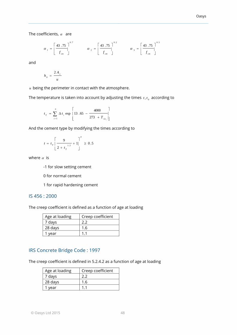
And t is he age of the concrete, 0
t the age of the concrete at the time of loading and H
a
coefficient depending on the relative humidity RH as a percentage and notional member size (in
mm) 0
h .
1500250012.015.10
18
hRHH
for 35cm
f
330
18
1500250012.015.1 hRHH
for 35cm
f
The coefficients, are
5.0
3
2.0
2
7.0
1
353535
cmcmcmfff
and
u
Ah
c2
0
u being the perimeter in contact with the atmosphere.
The temperature is taken into account by adjusting the times 0
, tt according to
i
t
n
i
iT
Ttt
273
4000exp
1
And the cement type by modifying the times according to
5.01
2
9
2.1
T
T
t
tt
where is
-1 for slow setting cement
0 for normal cement
1 for rapid hardening cement
AS 3600 – 2009
The creep coefficient is defined as
bcccckkkk
,5432
The basic creep coefficient bcc ,
is a function of concrete strength

Oasys
© Oasys Ltd 2015 44
Concrete strength, '
cf (MPa) 20 25 32 40 50 65 80 100
Basic creep coefficient bcc ,
5.2 4.2 3.4 2.8 2.4 2.0 1.7 1.5
And
htt
tk
15.08.0
8.0
2
2
h
t008.0exp12.10.12
3k is the maturity coefficient from Figure 3.1.8.3(B). This can be tabulated as
Age of concrete at time of loading Maturity coefficient 3
k
7 days 1.76
28 days 1.1
365 days 0.9
> 365 days 0.9
4k is the environmental coefficient
0.70 – arid
0.65 – interior
0.6 – temperate inland
0.5 – tropical or near coast
Concrete strength factor 5
k is
0.15k for MPaf
c50
'
'
3350.102.02
cfk for MPafMPa
c10050
'
With
24
3
7.0
k
Hong Kong Code of Practice
The creep coefficient is defined as
jecmLc
KKKKK

Oasys
© Oasys Ltd 2015 45
Where the factors are derived from code charts.
mK and
jK can be approximated by5
5 Allowance for creep under gradually applied loading, John Blanchard, 1998 NST 04

Oasys
© Oasys Ltd 2015 46
2
01 cLbLtK
m
with
Cement a b c
OPC 1.36 0.276 0.0132
RHPC 1.09 0.333 0.0366
and
0
0
0
tt
ttttKj
with
Effective
thickness (mm)
50 100 200 400 800
0.72 0.8 0.88 0.94 1
2.1 4.7 12.6 39.4 163
where 0
, tt are defined in weeks
ACI 209.2R-18
The creep coefficient is defined in Appendix A as
u
ttd
tttt
0
0
0,
Where t is the concrete age, 0
t the age at loading and d is the average thickness and are
constants for member shape and size.
,,,,,,0
35.2
ccscdcRHctcc
cu
with
118.0
00,25.1
ttc
for moist curing
094.0
00,13.1
ttc
for steam curing
hRHc
67.027.1,
for relative humidity, 4.0h
ddc
00092.014.1,
for 10
tt year
ddc
00067.010.1,
for 10
tt year

Oasys
© Oasys Ltd 2015 47
ssc
00264.082.0,
where s is the slump in mm
0024.088.0,
c
where is the ratio of fine to total aggregate
09.046.0 where is the air content in percent
IRC : 112-2011
The creep coefficient is defined as
000
,, tttt
with
00
tfcmRH
3
01.0
100/11
h
RH
RH
for 45
cmf
21
3
01.0
100/11
h
RH
RH for 45
cmf
cm
cm
f
f78.18
2.0
0
0
1.0
1
t
t
and
3.0
0
0
0,
tt
tttt
H
And t is he age of the concrete, 0
t the age of the concrete at the time of loading and H
a
coefficient depending on the relative humidity as a percentage and notional member size (in
mm) 0
h .
1500250012.015.10
18
hRHH
for 45cm
f
330
18
1500250012.015.1 hRHH
for 45cm
f 6
6 Code specifies a value of 35MPa, but 45MPa seems more correct.
Oasys
© Oasys Ltd 2015 48
The coefficients, are
5.0
3
2.0
2
7.0
1
75.4375.4375.43
cmcmcmfff
and
u
Ah
c2
0
u being the perimeter in contact with the atmosphere.
The temperature is taken into account by adjusting the times 0
, tt according to
i
t
n
i
iT
Ttt
273
400065.13exp
1
And the cement type by modifying the times according to
5.01
2
9
2.1
T
T
t
tt
where is
-1 for slow setting cement
0 for normal cement
1 for rapid hardening cement
IS 456 : 2000
The creep coefficient is defined as a function of age at loading
Age at loading Creep coefficient
7 days 2.2
28 days 1.6
1 year 1.1
IRS Concrete Bridge Code : 1997
The creep coefficient is defined in 5.2.4.2 as a function of age at loading
Age at loading Creep coefficient
7 days 2.2
28 days 1.6
1 year 1.1
Oasys
© Oasys Ltd 2015 49