Conceptualizing and Testing Random Indirect Effects … · Conceptualizing and Testing Random Indirect Effects and Moderated ... we would expect their scores on the outcome vari-

Conceptualizing and Testing Random Indirect Effects and ModeratedMediation in Multilevel Models: New Procedures

and Recommendations

Daniel J. Bauer, Kristopher J. Preacher, and Karen M. GilUniversity of North Carolina at Chapel Hill

The authors propose new procedures for evaluating direct, indirect, and total effects inmultilevel models when all relevant variables are measured at Level 1 and all effects arerandom. Formulas are provided for the mean and variance of the indirect and total effects andfor the sampling variances of the average indirect and total effects. Simulations show that theestimates are unbiased under most conditions. Confidence intervals based on a normalapproximation or a simulated sampling distribution perform well when the random effects arenormally distributed but less so when they are nonnormally distributed. These methods arefurther developed to address hypotheses of moderated mediation in the multilevel context. Anexample demonstrates the feasibility and usefulness of the proposed methods.

Keywords: multilevel model, hierarchical linear model, indirect effect, mediation, moderatedmediation

In psychology and other social sciences, hypotheses oftenconcern the causal pathways through which key predictorstransmit their effects to specific outcomes. For example,Wei, Mallinckrodt, Russell, and Abraham (2004) examinedthe extent to which attachment anxiety and avoidance wererelated to maladaptive perfectionism and, in turn, depressivemood. Similarly, Catanzaro and Laurent (2004) hypothe-sized that alcohol expectancies play a role in drinking as ameans of coping, which then predicts a number of drinkingbehaviors. In both of these cases, the causal effects of theoriginal predictor are transmitted at least partially throughan intervening variable, as diagrammed in Figure 1. In the

diagram, the product of the paths labeled a and b representsthe indirect effect of X on Y, the path labeled c� representsthe direct effect of X on Y, and c � ab � c� is the total effectof X on Y (Alwin & Hauser, 1975; Bollen, 1987, 1989).Depending on the pattern of these effects, the variable Mmay be called a mediator, a suppressor, or simply an inter-vening variable (MacKinnon, Krull, & Lockwood, 2000).We generally use the terms mediator and mediation to beconsistent with the focus of much of the literature on indi-rect effects, although our exposition also pertains to otherpatterns of indirect effects.

Within the context of linear regression and path analysis,a number of methods have been proposed for evaluatingmediation, and this remains an active area of research (e.g.,MacKinnon, Lockwood, Hoffman, West, & Sheets, 2002;MacKinnon, Lockwood, & Williams, 2004; Shrout &Bolger, 2002). Such methods are, however, inappropriate ifthe analyzed data are actually hierarchical in nature (i.e.,composed of two or more nested levels). Two forms ofhierarchical data are common in psychological research.First, individuals may be assessed from a number of groups.Individuals are then said to be nested within groups. To theextent that individuals within a group share common expe-riences, we would expect their scores on the outcome vari-able to be correlated across members of the group, whichviolates the independence assumption of many statisticalmodels. Second, repeated observations may be made on thesame individuals. In this case, the repeated measurementsare said to be nested within individuals. Repeated measure-ments are typically correlated within persons, which again

Daniel J. Bauer, Kristopher J. Preacher, and Karen M. Gil,Department of Psychology, University of North Carolina at ChapelHill.

Additional materials are on the Web at http://dx.doi.org/10.1037/1082-989X.11.2.142.supp

This work was funded in part by National Institute on DrugAbuse Grant F32 DA16883 awarded to Kristopher J. Preacher. Inaddition, the study of sickle cell disease that formed the basis ofthe applied analyses was supported by National Institutes of HealthGrant R01 HL6217 awarded to Karen M. Gil, principal investiga-tor. We also thank Greg Stonerock for assisting in the preparationof the sickle cell disease data and Li Cai for assisting with thetechnical appendix.

Correspondence concerning this article should be addressed toDaniel J. Bauer, Department of Psychology, Davie Hall 337-A,University of North Carolina at Chapel Hill, Chapel Hill, NC27599-3270. E-mail: [email protected]

Psychological Methods2006, Vol. 11, No. 2, 142–163

Copyright 2006 by the American Psychological Association1082-989X/06/$12.00 DOI: 10.1037/1082-989X.11.2.142

142

compromises the independence assumption. For both types ofhierarchical data, we refer to the lower level as Level 1 and theupper level as Level 2. More than two levels of data arepossible, but we restrict our attention to two-level models.

Because the independence assumption is violated forthese data structures, multiple linear regression and pathanalysis will produce biased tests of the effects in the model(Hox, 2002; Kreft & de Leeuw, 1998; Raudenbush & Bryk,2002). One way to appropriately model such data is to usea multilevel model, also known as a hierarchical linearmodel or a mixed-effects model. A key advantage of themultilevel model is that it captures the correlations amongthe Level 1 observations through the estimation of randomeffects. These random effects can take the form of randomintercepts, reflecting differences in the overall level of theoutcome variable across Level 2 units; random slopes, re-flecting differences in the effects of predictors across Level2 units; or both. For instance, a multilevel model with arandom intercept produces a compound symmetric correla-tion structure for the Level 1 observations. In addition to thestatistical advantages of multilevel models for correlateddata, random effects can have quite interesting substantiveinterpretations. A random slope, for example, indicates thatthe causal effect of the predictor on the outcome differs overLevel 2 units. This may then initiate the search for potentialmoderators of the effect.

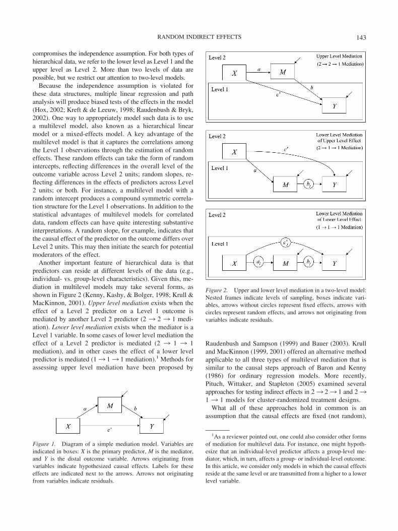
Another important feature of hierarchical data is thatpredictors can reside at different levels of the data (e.g.,individual- vs. group-level characteristics). Given this, me-diation in multilevel models may take several forms, asshown in Figure 2 (Kenny, Kashy, & Bolger, 1998; Krull &MacKinnon, 2001). Upper level mediation exists when theeffect of a Level 2 predictor on a Level 1 outcome ismediated by another Level 2 predictor (2 3 2 3 1 medi-ation). Lower level mediation exists when the mediator is aLevel 1 variable. In some cases of lower level mediation theeffect of a Level 2 predictor is mediated (2 3 1 3 1mediation), and in other cases the effect of a lower levelpredictor is mediated (13 13 1 mediation).1 Methods forassessing upper level mediation have been proposed by

Raudenbush and Sampson (1999) and Bauer (2003). Krulland MacKinnon (1999, 2001) offered an alternative methodapplicable to all three types of multilevel mediation that issimilar to the causal steps approach of Baron and Kenny(1986) for ordinary regression models. More recently,Pituch, Wittaker, and Stapleton (2005) examined severalapproaches for testing indirect effects in 23 23 1 and 231 3 1 models for cluster-randomized treatment designs.

What all of these approaches hold in common is anassumption that the causal effects are fixed (not random),

1As a reviewer pointed out, one could also consider other formsof mediation for multilevel data. For instance, one might hypoth-esize that an individual-level predictor affects a group-level me-diator, which, in turn, affects a group- or individual-level outcome.In this article, we consider only models in which the causal effectsreside at the same level or are transmitted from a higher to a lowerlevel variable.

Figure 1. Diagram of a simple mediation model. Variables areindicated in boxes: X is the primary predictor, M is the mediator,and Y is the distal outcome variable. Arrows originating fromvariables indicate hypothesized causal effects. Labels for theseeffects are indicated next to the arrows. Arrows not originatingfrom variables indicate residuals.

Figure 2. Upper and lower level mediation in a two-level model:Nested frames indicate levels of sampling, boxes indicate vari-ables, arrows without circles represent fixed effects, arrows withcircles represent random effects, and arrows not originating fromvariables indicate residuals.

143RANDOM INDIRECT EFFECTS

meaning that the magnitude of the effects is equal for allLevel 2 units. In lower level mediation, however, the causaleffects can be random because some predictors reside atLevel 1. In 23 13 1 mediation, the effect of the mediatoron the outcome may be random; in 1 3 1 3 1 mediation,all three causal effects can be random. These random effectsare indicated in Figure 2 as circles on the causal paths. Theyrepresent heterogeneity in the causal effects across Level 2units and may be of considerable substantive interest. Forinstance, in the empirical analysis to be presented later, weanalyze daily diary data to assess whether emotional reac-tions to pain mediate the relation between physical pain andstress in patients with sickle cell disease (SCD) and whetherthe strength of mediation differs across participants.

Kenny, Korchmaros, and Bolger (2003) first called atten-tion to the importance of random effects in lower levelmediation models, in particular in 1 3 1 3 1 models.Furthermore, they proposed a method for fitting 13 13 1models when all three causal pathways are random effects,as depicted in the lower panel of Figure 2. The purpose ofthe present article is to expand on this prior research toimprove the conceptualization and estimation of lower levelmediation with random effects in multilevel models. Webegin by showing how one can estimate the 1 3 1 3 1model simultaneously using conventional multilevel ormixed modeling software. We then clarify that, in the pres-ence of random indirect effects, one may be interested intwo related but different questions. First, is there heteroge-neity in the strength of the indirect, direct, and total effectsacross units of the population? Second, how precisely canwe estimate the average effects in the population? Afterdistinguishing these questions, we proceed to a small sim-ulation study designed to evaluate the quality of the averageeffect estimates and their confidence intervals (CIs). Next,we extend the model to include predictors of heterogeneityin the indirect and direct effects. Last, we demonstrate thevalue of estimating and predicting random indirect effects in1 3 1 3 1 models with an empirical example. Our focusthroughout is on the estimation and testing of the indirect,direct, and total effects of the distal predictor on the out-come, not on the broader causal steps approach to mediationoutlined by Baron and Kenny (1986).

Lower Level Mediation Models With RandomIndirect Effects

Loosely following the notation of Kenny et al. (2003),one can write the lower level mediation model depicted inthe lower panel of Figure 2 with two Level 1 equations as

Mij � dMj � ajXij � eMij

Yij � dYj � bjMij � c�j Xij � eYij . (1)

The terms eMij and eYij are Level 1 residuals for M and Y,respectively. The other five terms are interpreted similarlyto the intercepts and slopes of a standard regression model,with the caveat that each coefficient is random, meaning thatthe value of the coefficient varies across Level 2 units (asindicated by the j subscript). That is, the intercepts for Mand Y are designated dMj and dYj, respectively, the effect ofX on M is designated aj, the effect of M on Y is designatedbj, and the direct effect of X on Y is designated c�j . Therandom effects of the model permit heterogeneity in thecausal effects. For instance, if Level 1 represents repeatedmeasures, indexed by i, and Level 2 represents persons,indexed by j, then this model can be used to assess how thestrength of the hypothesized causal relations among X, M,and Y vary across individuals. For simplicity, we assume forthe time being that there are no Level 2 predictors of theserandom effects.

A number of assumptions are required to make the modelestimable and ensure that the effects are unbiased. Theseassumptions are inclusive of those that apply to all multi-level models (as conventionally estimated) but includefeatures that are unique to multivariate multilevel models,such as the lower level mediation model in Equation 1.These unique features are italicized in the following list ofassumptions:2

1. The predictors are uncorrelated with the random effects(intercepts and slopes) and residuals, both within and acrossequations (e.g., Xij must be uncorrelated with dMj, aj, andeMj and uncorrelated with dYj , bj , c�j , and eYij).

2. The residuals eMj and eYij are each normally distributedwith an expected value of zero, and they are uncorrelatedwith one another. Typically, the residuals for each outcomeare assumed to be independent and homoscedastic across iwithin j, but these restrictions can and should be relaxed incertain circumstances (e.g., when residuals are expected toautocorrelate with repeated measures). The additional as-sumption that the residuals are uncorrelated across out-comes is required to identify the effect of M on Y.

3. The random effects are normally distributed withmeans equal to the average effects in the population. Al-though other assumptions are possible, we also assume that

2 Another assumption that is sometimes listed for these modelsis that the predictors are fixed. This assumption seems to present aproblem for the model in Equation 1 because M appears in thesecond equation as a fixed predictor but also appears in the firstequation as a random outcome variable. Like ordinary regression,however, the assumption that the predictors are fixed is unneces-sary as long as the predictors are uncorrelated with the errors, aswe note in Assumption 1 (Demidenko, 2004, p. 143). We can thusconsider M to be a random variable in both equations. Conse-quently, we must now assume a distribution for M, namely that itis conditionally normal (conditional on the random effects and X),as indicated in Assumption 5.

144 BAUER, PREACHER, AND GIL

all of the random effects covary with one another. (Note thatthe random effects of a multilevel model are often expressedin deviation form, with the means subtracted, so that theexpected values of the random effects are zero.)

4. The Level 1 residuals are uncorrelated with the randomeffects both within and across equations (e.g., eMj is uncor-related with dMj, aj, dYj, bj, and c�j ).

5. Assumptions 2 and 3 imply that the distributions of Mand Y are conditionally normal. That is, the distribution ofM is normal conditional on X and the distribution of Y isnormal conditional on M and X.3

We show that Assumption 3 is particularly important forderiving estimates of the indirect effects. We can writeAssumption 3 more formally as

�dMj

aj

dYj

bj

c�j�

� N ��dM

adY

bc�

�, ��dMj

2

�dMj,aj�a

2j

�dMj,dYj�aj,dYj

�dYj

2

�dMj,bj�aj,bj

�dYj,bj�bj

2

�dMj,c�j �aj,c�j �dYj,c�j �bj,c�j �c�j2��. (2)

The means of the random effects are designated with thesame symbols as the random effects, absent the subscript jto indicate they are constant over Level 2 units (e.g., a is themean of aj). These are the fixed effects of the model. Thecovariance matrix for the random effects captures the non-independence of the observations collected at Level 1 and,together with the variances of the Level 1 residuals, consti-tutes the variance components of the model. The diagonalelements of this matrix, the variances, characterize hetero-geneity in the causal effects of the model across Level 2units. For instance, �c�j

2 is the variance of the direct effect�c�j ), indicating the extent to which the strength of the directeffect differs over Level 2 units. The off-diagonal elementsof the matrix capture the covariance among the randomeffects. For instance, a positive value for �aj,bj

would indi-cate that for Level 2 units for which the effect of X on M (aj)is high, the effect of M on Y (bj) is often also high.

To examine lower level mediation, Kenny et al. (2003)estimated each Level 1 model in Equation 1 separately.Unfortunately, this two-step approach sacrifices some im-portant information. First, one cannot estimate directly thecovariance of random effects residing in different Level 1models, including all of the elements enclosed in the dottedsquare in Equation 2. As we show, this makes it difficult tocapture the dispersion of the indirect and total effects of themodel. Kenny et al. (2003) proposed an ad hoc solution tothe problem that involved estimating ordinary least squares

regression models for M and Y separately for each unit j,collecting the slope estimates, and then calculating the sam-ple covariance of the slope estimates. They acknowledged,however, that this was not an optimal strategy. A secondlimitation of the two-step approach is that the asymptoticcovariance matrix of the model estimates is similarly in-complete. This matrix captures the sampling variability inthe estimates, and some of its missing elements are neededto capture the standard errors of the average indirect andtotal effects in the model.

The solution that we propose is to formulate the modelwith a single Level 1 equation through the use of selection(or indicator) variables. Researchers have used this strategyin the past to aid in the estimation of other kinds of multi-variate multilevel models (e.g., MacCallum, Kim, Malar-key, & Kiecolt-Glaser, 1997), and it is equally useful in thiscontext. The basic idea is to form a new outcome variable—for instance, Z—by stacking Y and M for each unit i withinj. This single outcome variable allows us to fit a “multivar-iate” model using univariate multilevel modeling software.To distinguish the two variables stacked in Z, we also createtwo selection variables—for instance, SM and SY. The vari-able SM is set equal to 1 when Z refers to M and is 0otherwise. Similarly, the variable SY is set equal to 1 whenZ refers to Y and is 0 otherwise. We retain the variables Xand M in the new data set, as they are needed as predictorsof Z. An example of this data rearrangement is presented inFigure 3.

The purpose of rearranging the data in this fashion is thatwe can now specify the lower level mediation model with asingle equation:

Zij � SMij�dMj � ajXij� � SYij

�dYj � bjMij � c�j Xij� � eZij. (3)

Notice that the two selection variables essentially togglefrom the model for M to the model for Y in Equation 3. Forinstance, when Z is a value of M, then SM � 1 and SY � 0,and Equation 3 simplifies to Zij � dMj � ajXij � eZij . Thisis the model for M from Equation 1. Similarly, when Z is avalue of Y, then SY � 1 and SM � 0, and Equation 3simplifies to Zij � dYj � bjMij � c�j Xij � eZij , or the modelfor Y from Equation 1. Thus, although we have stacked Yand M into a single dependent variable for the purpose of

3 A reviewer correctly noted that the unconditional joint distri-bution of M and Y would not be normal, given the contribution ofthe ajbj product to Y. However, it is important to note that theconditional distribution of M given X and Y given M and X can stillbe normal and that it is this conditional distribution for whichnormality is assumed. Although this assumption is common to alllinear multilevel models, it may often be unrealistic in practice.Therefore, in our simulation study, we consider the consequencesof violating this assumption when the random effects are nonnor-mally distributed.


fitting the model, the two outcomes continue to be distin-guished in the model equations by the selection variables.

To aid in specifying the model, it is helpful to distributethe selection variables in Equation 3 as follows:

Zij � dMjSMij � aj�SMijXij� � dYjSYij

� bj�SYijMij� � c�j (SYij

Xij) � eZij . (4)

Equation 4 shows that one would specify a model for Z withno intercept but with random effects for SM and SY (dMj anddYj, respectively) and with random effects for the productvariables SMX, SYM, and SYX (aj, bj, and c�j , respectively). Inaddition, one must use some method to allow the residualvariance Var(eZij) to differ depending on SM (or, equiva-lently, SY). This represents a form of heteroscedasticitybecause the residual variance for Z is then conditional onSM. Fortunately, most multilevel modeling software pro-grams offer one or more options for modeling heterosce-dasticity. Depending on the substantive context, more com-plicated Level 1 residual variance (or covariance) structurescan also be entertained (see the example we provide later in the

article). Generic syntax for rearranging the data and fittingthe model in Equation 4 in SAS is provided on the Webat http://dx.doi.org/10.1037/1082-989X.11.2.142.supp, al-though other programs, such as SPSS, HLM, or MLwiN,could also be used to fit the model.

Note that this specification strategy generalizes to modelswith more than one mediator through the creation of addi-tional selection variables. The key is to “trick” the softwareinto estimating a multivariate system of equations throughthe creation of a single outcome variable Z. Given thisset-up, one can estimate the entire model simultaneouslyusing conventional software for univariate multilevel mod-els. The resulting output includes the full covariance matrixof the random effects and the full asymptotic covariancematrix of the fixed effects estimates and variance compo-nents, both of which are critical for our next developments.

To summarize to this point, we note that by using theselection variable approach, we can estimate the completelower level mediation model simultaneously, providing allof the necessary information for evaluating the hypothe-sized causal effects of the model. We now turn to methodsfor quantifying and testing variability in these causal effects.

Evaluating Random Indirect and Total Effects inMultilevel Models

In this section, we consider two related questions: Giventhe presence of random effects in a lower level mediationmodel, how does one quantify variability in the indirect andtotal effects across Level 2 units of the population, and howdoes one obtain CIs for the average indirect and totaleffects? Although these are related questions, they are quitedifferent in purpose. For the first question, we are interestedin variability across Level 2 units (i.e., heterogeneity incausal effects). For the second question, we are interested invariability in our estimates of the average effects acrossLevel 2 units (i.e., the precision of the average causaleffects). This distinction is analogous to the difference be-tween the standard deviation of a variable and the standarderror of its mean. We now present the technical details forevaluating each question. Additional details on the deriva-tion of the results presented in this section are provided inthe Appendix. Readers who wish to see only the conclusionsof these developments can skip to the Summary of Proce-dures subsection.

Investigating Heterogeneity in Causal Effects

The first question concerns how to characterize heteroge-neity in the causal effects over Level 2 units. Let us considerthe indirect effect first. The indirect effect for a given unit jis ajbj. As Kenny et al. (2003) noted, because aj and bj arenot necessarily independent, the expected value or averageof ajbj is (Goodman, 1960, p. 712):

Figure 3. In the top diagram, data are shown for two upper levelunits (j � 1 and j � 2) for an outcome (Y), a mediator (M), and apredictor (X) whose effect on Y is thought to be mediated by M.This data set is then rearranged into the lower diagram through thecreation of a new variable Z that represents Y whenever theselection variable SY � 1 (and SM � 0) and represents M wheneverthe selection variable SM � 1 (and SY � 0). For each observationin the top diagram, there are then two rows in the bottom diagram.The values of M and X are repeated for these two rows.


E�ajbj� � ab � �aj ,bj. (5)

As such, the average indirect effect in the population is afunction of the average effect of X on M (or a), the averageeffect of M on Y (or b), and the covariance between the tworandom effects (or �aj ,bj

). One interesting implication of thisformula is that even if a and b are zero, the average indirecteffect can be nonzero through the contribution of �aj ,bj

. Wenote that this formula does not require any assumptions onthe distributions of the random effects (Kendall & Stuart,1969, p. 283).

Making the assumption that aj and bj are normally dis-tributed, Kenny et al. (2003) showed that the variance ofajbj is

Var�ajbj� � b2�aj

2 � a2�bj

2 � �aj

2 �bj

2 � 2ab�aj ,bj� �aj ,bj

2 . (6)

This variance quantifies heterogeneity in the strength of theindirect effect at Level 2. This value may be of considerableinterest, as it indicates the extent to which the indirect effectof X on Y varies across the Level 2 sampling units. Simi-larly, Kenny et al. (2003) noted that the average total effect,ajbj �c�j , can be expressed as

E�ajbj � c�j � � ab � �aj ,bj� c�. (7)

Again with the assumption of normality of the randomeffects, the variance of the random total effect can beexpressed as

Var�ajbj � c�j � � b2�aj

2 � a2�bj

2 � �aj

2 �bj

2 � 2ab�aj ,bj

� �aj ,bj

2 � �c�j2 � 2b�aj ,c�j � 2a�bj ,c�j . (8)

This variance, in turn, quantifies heterogeneity at Level 2 inthe strength of the total effect.

One nice property of maximum likelihood estimation, thetypical method for fitting multilevel models, is that anyfunction of maximum likelihood estimates (MLEs) is itselfan MLE (Raudenbush & Bryk, 2002, p. 52). As such, wecan obtain MLEs for the quantities in Equations 5 through8 by inserting the estimates from the fitted model in place oftheir population values. The simultaneous modeling ap-proach we have described generates all of these estimatesfrom a single model. Of particular interest may be theestimated average indirect and total effects, which we canobtain by inserting the model estimates into Equations 5 and7. Our second question is concerned with the precision ofthese estimated average indirect and total effects.

Quantifying the Precision of the Estimated AverageCausal Effects

We begin by emphasizing that Equations 6 and 8 captureheterogeneity in the indirect effects and total effects in thepopulation of Level 2 units.4 If we are instead interested in

the precision of the estimated average indirect effect, ab ��aj ,bj

, and estimated average total effect, ab � �aj ,bj� c�j ,

then we can calculate the sampling variances of these esti-mates as

Var�ab � �aj ,bj� � b2Var�a� � a2Var(b)

� Var�a�Var�b� � 2abCov�a, b�

� Cov�a, b�2 � Var��aj ,bj� (9)

and

Var�ab � �aj ,bj� c�� b2Var�a� � a2Var�b�

� Var�a�Var�b� � 2abCov�a, b� � Cov�a, b�2 � Var�c��

� 2bCov�a, c�� 2aCov�b, c�� Var ��aj ,bj�. (10)

The variances and covariances in these equations (desig-nated Var and Cov) represent the asymptotic samplingvariances and covariances of the fixed effect estimates a, b,and c� and the covariance estimate �aj ,bj

.In practice, one must replace the population values in

Equations 9 and 10 with their sample estimates (the modelestimates and estimated asymptotic variances and covari-ances of the estimates) to obtain the estimated samplingvariances of the average direct and indirect effects. Mostmultilevel or mixed modeling software programs provide anoption to output the estimated variance–covariance matrixof the model estimates. Note that only by estimating the fullmodel simultaneously can one estimate covariances be-tween fixed effects residing in different equations—for ex-ample, Cov(a, b) and Cov(a, c�).

To make inferences concerning the average indirect andtotal effects, we can form CIs for the estimates. One methodfor constructing CIs assumes normality for the samplingdistributions of the estimates. Under this assumption, 95%CIs for the average indirect effect and average total effectare obtained as

�ab � �aj ,bj� � 1.96 �Var�ab � �aj ,bj

��1/ 2 (11)

and

�ab � �aj ,bj� c�� 1.96 �Var�ab � �aj ,bj

� c��1/ 2, (12)

where �1.96 is the critical value of the z distribution and

Var is used to indicate the estimated sampling varianceobtained when the sample-based estimates are inserted into

4 Kenny et al. (2003) sometimes interpreted these equations togive the sampling variances of the estimated average indirect andtotal effects.


Equation 9 or 10. Alternatively, one could perform a nullhypothesis test by forming the critical ratio of each estimateto its standard error and comparing the result with thecritical value of the z distribution. In either case, the as-sumption of normality for the sampling distributions willnot hold exactly, given that ab is a product of normallydistributed estimates (and hence will not be normal). Thedeviation from normality may be small enough, however,that the CIs or significance tests will still be reasonablyaccurate.

An alternative method for constructing CIs that may holdpromise is the Monte Carlo (MC) method of MacKinnon etal. (2004). In this approach, the sampling distribution for theeffect of interest is not assumed to be normal and is insteadsimulated from the model estimates and their asymptoticvariances and covariances (a form of parametric bootstrap-ping). For instance, to simulate the sampling distribution ofthe average indirect effect, one would define a multinormaldistribution with means equal to a, b, and �aj ,bj

and covari-ance matrix equal to the estimated covariance matrix ofthese estimates. One would then take random values fromthis multinormal distribution and plug them into Equation 5to compute the average indirect effect. Collecting the resultsover many draws provides a simulated sampling distributionfor the average indirect effect. One would then obtain con-fidence limits for the average indirect effect by taking thecorresponding percentiles of this simulated sampling distri-bution (e.g., 2.5th and 97.5th for a 95% CI). The advantageof this approach is that it does not assume normality for thesampling distributions of the average indirect and totaleffects.

Summary of Procedures

In conclusion, when one estimates lower level mediationmodels with random effects, interest may center on both theaverage causal effects and potential heterogeneity in thesecausal effects across the Level 2 units of the population. Theaverage indirect and total effects can be computed viaEquations 5 and 7. Estimates obtained from these equationsindicate the strength of the indirect and total effects for anaverage Level 2 unit in the population. Allowing the indirectand total effects to be random, however, also implies thatthere is variability about these average values across Level2 units. This heterogeneity in the strength of the indirect andtotal effects in the population can be characterized by thevariance formulas given in Equations 6 and 8. Therefore, forinstance, the variance obtained from Equation 6 indicatesthe extent to which the magnitude of the indirect effectdiffers across Level 2 units.

We have also suggested two possible ways to makeinferences for the average indirect and total effect estimates.In the first approach, the standard errors of the averageindirect and total effects are computed as the square roots of

Equations 9 and 10. One can then use these standard errorsto form CIs (or significance tests) by assuming that theestimates of the average indirect and total effects havenormal sampling distributions, as shown in Equations 11and 12. A second approach is to simulate the samplingdistributions of the average indirect and total effects. Thissecond approach is more difficult to implement, but it hasthe advantage that the simulated sampling distributions ofthe average indirect and total effect estimates will have thetheoretically correct (nonnormal) forms. Both tests are im-plemented in a SAS macro available on the Web at http://dx.doi.org/10.1037/1082-989X.11.2.142.supp. Given thetrade-offs involved, we now turn to a comparison of theperformance of these two alternative procedures for makinginferences about the average indirect and total effects.

Performance With Simulated Data

As a preliminary investigation of the accuracy of theestimates and CIs just described, we conducted a modestsimulation study based on the example presented in Kennyet al. (2003, pp. 122–123). In their example, the randomintercept for the M equation, dMj, had a mean of 0 and avariance of .6, and the random intercept for the Y equation,dYj, had a mean of zero and a variance of .4. These tworandom effects were normally distributed and were uncor-related with each other and with the other random effects inthe model. For the M equation, the Level 1 residual variancewas set to �eM

2 � .65; for the Y equation, it was set to�eY

2 � .45. The causal paths were simulated as follows: aj

and bj were both normally distributed with means of a �b � .6 and variances of �aj

2 � �bj

2 � .16 and c�j wasnormally distributed with a mean of c� � .2 and a varianceof �c� j

2 � .04. The covariance between aj and bj was �aj ,bj

� .113, yielding a correlation of .706. Neither aj nor bj wascorrelated with c�j . Last, the predictor X was simulated fromthe equation Xij � X� j � eXij , where X� j � N �0, 1� andeXij � N �0, 1�.

To generate our own simulated data, we used this modelas a base from which we varied four design factors. Invarying these factors, we focused specifically on how theymight influence the average indirect effect estimate, as thiseffect is typically of most interest (results differed little forthe average total effect). We chose the first two factors ofthe simulation study to manipulate the effect size of theaverage indirect effect as expressed in Equation 5. First, themagnitude of the a and b parameters was set to either a �b � .3 or a � b � .6. The higher values for a and b areidentical to those used by Kenny et al. (2003), whereas thelower values are close to the smaller effect sizes consideredby Krull and MacKinnon (2001) for similar models. Thesecond design factor was the magnitude of the covariancebetween aj and bj. This parameter was set to one of threevalues, �aj ,bj

� � .113, 0, or .113 (correlations of .706,


.000, and .706, respectively). The next two design factorsmanipulated the total sample size. We first set the number ofLevel 2 units to N � 25, 50, 100, or 200. We then set thenumber of observations per Level 2 unit to nj � 4, 8, 16, or32. These sample sizes are consistent with those used byKrull and MacKinnon (2001). The final design factor con-cerned the distributions of the random effects aj and bj. Toevaluate the robustness of the estimates, we simulated aj andbj either from normal distributions or from �2(3) distribu-tions, having skew 1.63 and kurtosis 4.

Together, these four factors combined to yield 144 con-ditions in a fully factorial design. In addition, to investigateType I errors, we simulated supplemental data where a �b � 0 and �aj ,bj

� 0 at each sample size and for bothdistributional conditions, which resulted in an additional 24conditions. Within each cell of the design, we simulated 500samples of data, which resulted in a total of 84,000 repli-cations (further details on the data generation are availablefrom Daniel J. Bauer on request). We then fitted the modelspecified in Equation 4 to each data set using SAS PROCMIXED with the restricted maximum likelihood estimatorand a maximum of 1,000 iterations.

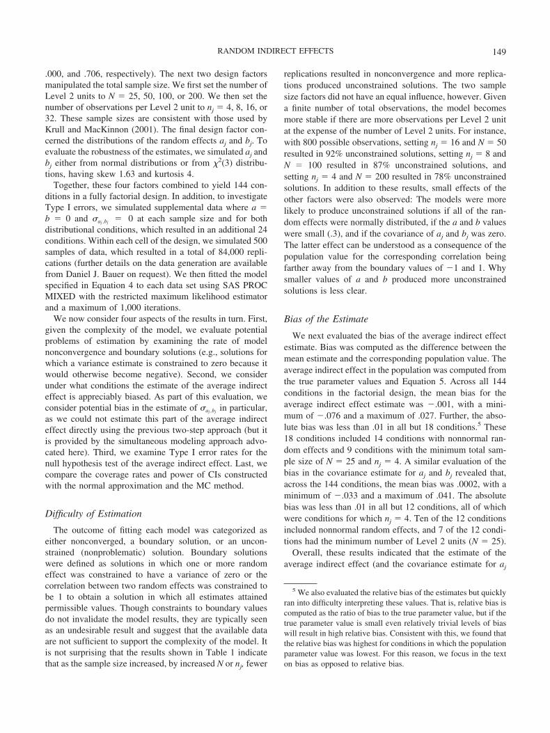
We now consider four aspects of the results in turn. First,given the complexity of the model, we evaluate potentialproblems of estimation by examining the rate of modelnonconvergence and boundary solutions (e.g., solutions forwhich a variance estimate is constrained to zero because itwould otherwise become negative). Second, we considerunder what conditions the estimate of the average indirecteffect is appreciably biased. As part of this evaluation, weconsider potential bias in the estimate of �aj ,bj

in particular,as we could not estimate this part of the average indirecteffect directly using the previous two-step approach (but itis provided by the simultaneous modeling approach advo-cated here). Third, we examine Type I error rates for thenull hypothesis test of the average indirect effect. Last, wecompare the coverage rates and power of CIs constructedwith the normal approximation and the MC method.

Difficulty of Estimation

The outcome of fitting each model was categorized aseither nonconverged, a boundary solution, or an uncon-strained (nonproblematic) solution. Boundary solutionswere defined as solutions in which one or more randomeffect was constrained to have a variance of zero or thecorrelation between two random effects was constrained tobe 1 to obtain a solution in which all estimates attainedpermissible values. Though constraints to boundary valuesdo not invalidate the model results, they are typically seenas an undesirable result and suggest that the available dataare not sufficient to support the complexity of the model. Itis not surprising that the results shown in Table 1 indicatethat as the sample size increased, by increased N or nj, fewer

replications resulted in nonconvergence and more replica-tions produced unconstrained solutions. The two samplesize factors did not have an equal influence, however. Givena finite number of total observations, the model becomesmore stable if there are more observations per Level 2 unitat the expense of the number of Level 2 units. For instance,with 800 possible observations, setting nj � 16 and N � 50resulted in 92% unconstrained solutions, setting nj � 8 andN � 100 resulted in 87% unconstrained solutions, andsetting nj � 4 and N � 200 resulted in 78% unconstrainedsolutions. In addition to these results, small effects of theother factors were also observed: The models were morelikely to produce unconstrained solutions if all of the ran-dom effects were normally distributed, if the a and b valueswere small (.3), and if the covariance of aj and bj was zero.The latter effect can be understood as a consequence of thepopulation value for the corresponding correlation beingfarther away from the boundary values of 1 and 1. Whysmaller values of a and b produced more unconstrainedsolutions is less clear.

Bias of the Estimate

We next evaluated the bias of the average indirect effectestimate. Bias was computed as the difference between themean estimate and the corresponding population value. Theaverage indirect effect in the population was computed fromthe true parameter values and Equation 5. Across all 144conditions in the factorial design, the mean bias for theaverage indirect effect estimate was .001, with a mini-mum of .076 and a maximum of .027. Further, the abso-lute bias was less than .01 in all but 18 conditions.5 These18 conditions included 14 conditions with nonnormal ran-dom effects and 9 conditions with the minimum total sam-ple size of N � 25 and nj � 4. A similar evaluation of thebias in the covariance estimate for aj and bj revealed that,across the 144 conditions, the mean bias was .0002, with aminimum of .033 and a maximum of .041. The absolutebias was less than .01 in all but 12 conditions, all of whichwere conditions for which nj � 4. Ten of the 12 conditionsincluded nonnormal random effects, and 7 of the 12 condi-tions had the minimum number of Level 2 units (N � 25).

Overall, these results indicated that the estimate of theaverage indirect effect (and the covariance estimate for aj

5 We also evaluated the relative bias of the estimates but quicklyran into difficulty interpreting these values. That is, relative bias iscomputed as the ratio of bias to the true parameter value, but if thetrue parameter value is small even relatively trivial levels of biaswill result in high relative bias. Consistent with this, we found thatthe relative bias was highest for conditions in which the populationparameter value was lowest. For this reason, we focus in the texton bias as opposed to relative bias.


and bj) was largely unbiased except for a few of the non-normal random effects or very small sample conditions. It isnoteworthy that these are also the conditions for which itwas difficult to estimate the model, which provides con-verging evidence that we need larger samples to obtainreliable results.

Type I Errors

Using the 24 supplementary cells of the simulation designfor which the population value of the average indirect effectwas zero, we next considered the Type I error rates for testsof the average indirect effect (setting the nominal error rateat 5%). We calculated 95% CIs using the normal approxi-mation in Equation 11 and the MC method of MacKinnon etal. (2004). The latter method involved taking 50,000 ran-dom draws from the estimated sampling distribution of theestimates (i.e., the multivariate normal sampling distribu-tion of a, b, and �aj ,bj

), calculating Equation 5 for eachdraw, and then computing the 2.5th and 97.5th percentilesof the resulting values. Both the normal approximation andthe MC method require an estimate of the covariance matrixof the fixed effects (e.g., a and b). Typically, one computesthese values by taking the inverse of the information matrixfor the estimates. For multilevel models, however, this

procedure is known to underestimate the sampling variabil-ity of the fixed effect estimates because the variance com-ponents of the model are treated as known (when they are,in fact, estimated). Kackar and Harville (1984) provided amethod for inflating the elements of the covariance matrixof the fixed effects to correct for this bias. We compare theCIs we obtained by using the default covariance matrix ofthe fixed effects versus the inflated Kackar–Harville (K-H)covariance matrix of the fixed effects. To do so, we calcu-lated Type I error rates as the percentage of replications inwhich the 95% CI for the average indirect effect failed tocover zero.

Tables 2 and 3 compare the Type I error rates for the fourtypes of CIs for normally and nonnormally distributed ran-dom effects, respectively. The results indicate that all fourCIs tended to produce Type I error rates below the nominallevel, especially at the lower sample sizes. CIs based on theMC method, however, reflected the nominal Type I errorrate better than the other CIs. Further examination of thedata indicated that, at the smallest sample sizes, the standarderrors of the average indirect effect estimate were overesti-mated, producing CIs that were too wide and thus morelikely to include zero. We now consider whether this is alsothe case when the null hypothesis is false.

Table 1Result of Fitting the Lower Level Mediation Model With Random Causal Effects as a Functionof the Number of Level 2 Units (N) and the Number of Level 1 Units Within Each Level 2 Unit(nj)

Observations

Result of model fitting (% of replications)

Failed toconverge

Boundarysolution

Unconstrainedsolution

N � 25

nj � 4 93.03 4.90 2.07nj � 8 56.63 23.10 20.27nj � 16 16.18 23.02 60.80

N � 50

nj � 4 54.70 26.93 18.37nj � 8 13.93 28.10 57.97nj � 16 1.18 6.72 92.10

N � 100

nj � 4 16.52 34.13 49.35nj � 8 1.80 10.97 87.23nj � 16 0.37 0.67 98.97

N � 200

nj � 4 2.50 19.52 77.98nj � 8 0.58 1.70 97.72nj � 16 0.27 0.00 99.73

Note. Results are collapsed over conditions that vary in the population parameter values and in the distributionsof the random effects (normal or nonnormal).


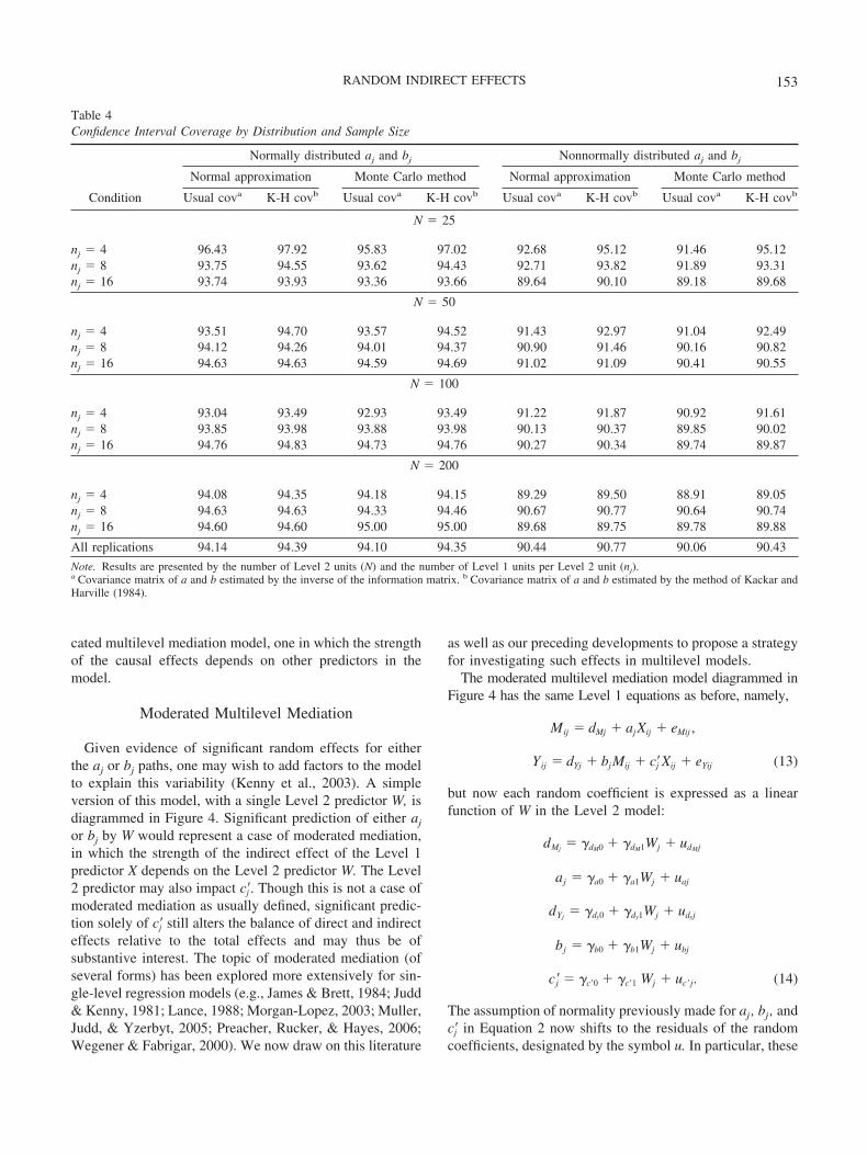
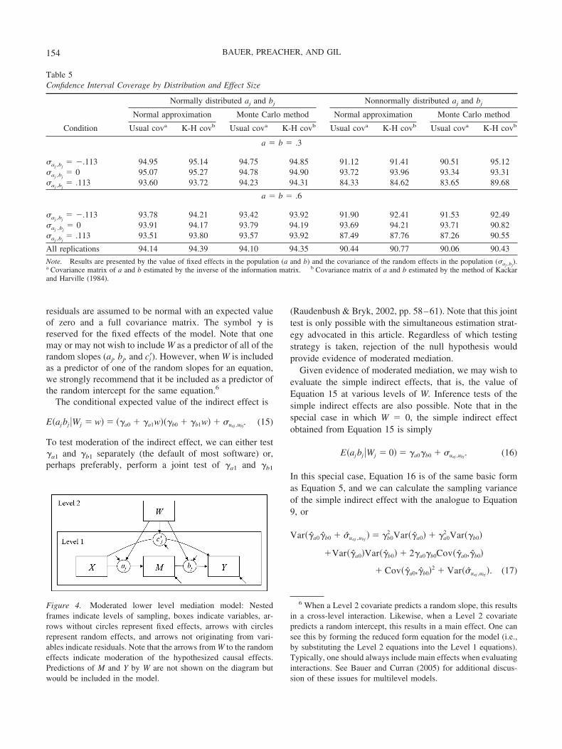
CI Coverage Rates

Coverage rates for the CIs are presented in Table 4 bysample size and in Table 5 by the magnitude of the param-eter values in the population model. Consistent with theresults on Type I errors, the CIs were too wide in thesmallest sample condition (N � 25, nj � 4) when therandom effects were normal. Outside of this condition,however, the CIs actually tended to be too narrow, produc-ing slightly lower than 95% coverage of the true populationparameter values. The dominant factor determining the cov-erage rates of the CIs was the distribution of the randomeffects. In general, regardless of the method for computingthe CIs, the coverage rates hovered around 94% when therandom effects were normally distributed and dropped toabout 90% when the random effects were nonnormallydistributed. The lower coverage rates for the nonnormalconditions reflected a general underestimation of the sam-pling variances of all of the estimates in the model.

Tables 4 and 5 also point to some clear differences betweenmethods for computing the CIs. Across replications, the CIsconstructed via Equation 11 performed slightly better thanthose computed via the MC method. This advantage of thenormal approximation method was seen for 105 of 144conditions (73%) but was stronger when the random effectswere nonnormal. Additionally, Tables 4 and 5 show that theK-H covariance matrix of the fixed effects produced CIswith better coverage rates. Overall, we attained the bestcoverage rates by combining the normal approximation ofEquation 11 with the K-H procedure. The MC method withthe K-H procedure performed nearly as well.

Finally, Tables 4 and 5 indicate that the effect of nonnor-mal random effects on the coverage rates of the CIs wasmoderated by several factors. First, the coverage rates wereslightly better at the smallest sample sizes (low N combinedwith low nj). Second, the coverage rates were least affectedby nonnormality when the covariance of the random effects

Table 2Type I Error Rates: Normal Random Effects

Condition Replicationsa

Normal approximation Monte Carlo method

Usual covb K-H covc Usual covb K-H covc

N � 25

1. nj � 4 70 0.00 0.00 0.00 0.002. nj � 8 337 2.97 2.97 5.34 5.343. nj � 16 484 2.48 2.48 4.34 4.13

N � 50

4. nj � 4 351 4.27 4.27 4.84 4.565. nj � 8 486 3.70 3.70 4.12 4.126. nj � 16 500 3.20 3.20 4.20 4.20

N � 100

7. nj � 4 482 4.98 4.98 5.39 5.398. nj � 8 499 4.41 4.41 4.61 4.619. nj � 16 500 6.00 6.00 6.20 6.00

N � 200

10. nj � 4 500 4.00 4.00 4.00 4.0011. nj � 8 500 6.00 6.00 6.20 6.2012. nj � 16 500 4.80 4.60 5.00 4.60

Collapsing

1 through 12 5,209 4.24 4.22 4.86 4.762 through 12 5,139 4.30 4.28 4.92 4.834 through 12 4,318 4.61 4.59 4.96 4.86

Note. Results are presented by the number of Level 2 units (N) and the number of Level 1 units per Level 2unit (nj). The nominal Type I error rate was set at 5%.a Number of replications resulting in a converged solution from which Type I error rates were calculated (outof 500, except for results collapsed over conditions). b Covariance matrix of a and b estimated by the inverseof the information matrix. c Covariance matrix of a and b estimated by the method of Kackar and Harville(1984).


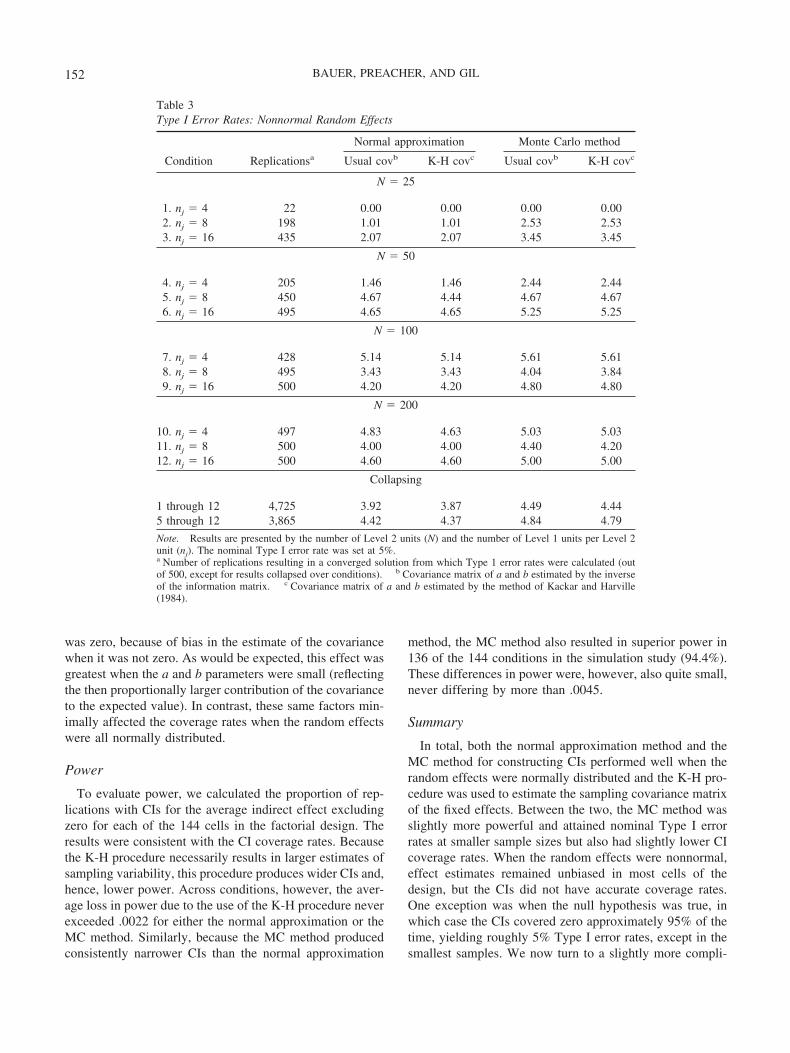
was zero, because of bias in the estimate of the covariancewhen it was not zero. As would be expected, this effect wasgreatest when the a and b parameters were small (reflectingthe then proportionally larger contribution of the covarianceto the expected value). In contrast, these same factors min-imally affected the coverage rates when the random effectswere all normally distributed.

Power

To evaluate power, we calculated the proportion of rep-lications with CIs for the average indirect effect excludingzero for each of the 144 cells in the factorial design. Theresults were consistent with the CI coverage rates. Becausethe K-H procedure necessarily results in larger estimates ofsampling variability, this procedure produces wider CIs and,hence, lower power. Across conditions, however, the aver-age loss in power due to the use of the K-H procedure neverexceeded .0022 for either the normal approximation or theMC method. Similarly, because the MC method producedconsistently narrower CIs than the normal approximation

method, the MC method also resulted in superior power in136 of the 144 conditions in the simulation study (94.4%).These differences in power were, however, also quite small,never differing by more than .0045.

Summary

In total, both the normal approximation method and theMC method for constructing CIs performed well when therandom effects were normally distributed and the K-H pro-cedure was used to estimate the sampling covariance matrixof the fixed effects. Between the two, the MC method wasslightly more powerful and attained nominal Type I errorrates at smaller sample sizes but also had slightly lower CIcoverage rates. When the random effects were nonnormal,effect estimates remained unbiased in most cells of thedesign, but the CIs did not have accurate coverage rates.One exception was when the null hypothesis was true, inwhich case the CIs covered zero approximately 95% of thetime, yielding roughly 5% Type I error rates, except in thesmallest samples. We now turn to a slightly more compli-

Table 3Type I Error Rates: Nonnormal Random Effects

Condition Replicationsa

Normal approximation Monte Carlo method

Usual covb K-H covc Usual covb K-H covc

N � 25

1. nj � 4 22 0.00 0.00 0.00 0.002. nj � 8 198 1.01 1.01 2.53 2.533. nj � 16 435 2.07 2.07 3.45 3.45

N � 50

4. nj � 4 205 1.46 1.46 2.44 2.445. nj � 8 450 4.67 4.44 4.67 4.676. nj � 16 495 4.65 4.65 5.25 5.25

N � 100

7. nj � 4 428 5.14 5.14 5.61 5.618. nj � 8 495 3.43 3.43 4.04 3.849. nj � 16 500 4.20 4.20 4.80 4.80

N � 200

10. nj � 4 497 4.83 4.63 5.03 5.0311. nj � 8 500 4.00 4.00 4.40 4.2012. nj � 16 500 4.60 4.60 5.00 5.00

Collapsing

1 through 12 4,725 3.92 3.87 4.49 4.445 through 12 3,865 4.42 4.37 4.84 4.79

Note. Results are presented by the number of Level 2 units (N) and the number of Level 1 units per Level 2unit (nj). The nominal Type I error rate was set at 5%.a Number of replications resulting in a converged solution from which Type 1 error rates were calculated (outof 500, except for results collapsed over conditions). b Covariance matrix of a and b estimated by the inverseof the information matrix. c Covariance matrix of a and b estimated by the method of Kackar and Harville(1984).


cated multilevel mediation model, one in which the strengthof the causal effects depends on other predictors in themodel.

Moderated Multilevel Mediation

Given evidence of significant random effects for eitherthe aj or bj paths, one may wish to add factors to the modelto explain this variability (Kenny et al., 2003). A simpleversion of this model, with a single Level 2 predictor W, isdiagrammed in Figure 4. Significant prediction of either aj

or bj by W would represent a case of moderated mediation,in which the strength of the indirect effect of the Level 1predictor X depends on the Level 2 predictor W. The Level2 predictor may also impact c�j . Though this is not a case ofmoderated mediation as usually defined, significant predic-tion solely of c�j still alters the balance of direct and indirecteffects relative to the total effects and may thus be ofsubstantive interest. The topic of moderated mediation (ofseveral forms) has been explored more extensively for sin-gle-level regression models (e.g., James & Brett, 1984; Judd& Kenny, 1981; Lance, 1988; Morgan-Lopez, 2003; Muller,Judd, & Yzerbyt, 2005; Preacher, Rucker, & Hayes, 2006;Wegener & Fabrigar, 2000). We now draw on this literature

as well as our preceding developments to propose a strategyfor investigating such effects in multilevel models.

The moderated multilevel mediation model diagrammed inFigure 4 has the same Level 1 equations as before, namely,

Mij � dMj � ajXij � eMij ,

Yij � dYj � bjMij � c�j Xij � eYij (13)

but now each random coefficient is expressed as a linearfunction of W in the Level 2 model:

dMj� �dM0 � �dM1Wj � udMj

aj � �a0 � �a1Wj � uaj

dYj� �dy0 � �dy1Wj � udyj

bj � �b0 � �b1Wj � ubj

c�j � �c�0 � �c�1 Wj � uc�j. (14)

The assumption of normality previously made for aj , bj , andc�j in Equation 2 now shifts to the residuals of the randomcoefficients, designated by the symbol u. In particular, these

Table 4Confidence Interval Coverage by Distribution and Sample Size

Condition

Normally distributed aj and bj Nonnormally distributed aj and bj

Normal approximation Monte Carlo method Normal approximation Monte Carlo method

Usual cova K-H covb Usual cova K-H covb Usual cova K-H covb Usual cova K-H covb

N � 25

nj � 4 96.43 97.92 95.83 97.02 92.68 95.12 91.46 95.12nj � 8 93.75 94.55 93.62 94.43 92.71 93.82 91.89 93.31nj � 16 93.74 93.93 93.36 93.66 89.64 90.10 89.18 89.68

N � 50

nj � 4 93.51 94.70 93.57 94.52 91.43 92.97 91.04 92.49nj � 8 94.12 94.26 94.01 94.37 90.90 91.46 90.16 90.82nj � 16 94.63 94.63 94.59 94.69 91.02 91.09 90.41 90.55

N � 100

nj � 4 93.04 93.49 92.93 93.49 91.22 91.87 90.92 91.61nj � 8 93.85 93.98 93.88 93.98 90.13 90.37 89.85 90.02nj � 16 94.76 94.83 94.73 94.76 90.27 90.34 89.74 89.87

N � 200

nj � 4 94.08 94.35 94.18 94.15 89.29 89.50 88.91 89.05nj � 8 94.63 94.63 94.33 94.46 90.67 90.77 90.64 90.74nj � 16 94.60 94.60 95.00 95.00 89.68 89.75 89.78 89.88

All replications 94.14 94.39 94.10 94.35 90.44 90.77 90.06 90.43

Note. Results are presented by the number of Level 2 units (N) and the number of Level 1 units per Level 2 unit (nj).a Covariance matrix of a and b estimated by the inverse of the information matrix. b Covariance matrix of a and b estimated by the method of Kackar andHarville (1984).


residuals are assumed to be normal with an expected valueof zero and a full covariance matrix. The symbol � isreserved for the fixed effects of the model. Note that onemay or may not wish to include W as a predictor of all of therandom slopes (aj, bj, and c�j ). However, when W is includedas a predictor of one of the random slopes for an equation,we strongly recommend that it be included as a predictor ofthe random intercept for the same equation.6

The conditional expected value of the indirect effect is

E�ajbj �Wj � w� � ��a0 � �a1w��b0 � �b1w� � �uaj ,ubj. (15)

To test moderation of the indirect effect, we can either test�a1 and �b1 separately (the default of most software) or,perhaps preferably, perform a joint test of �a1 and �b1

(Raudenbush & Bryk, 2002, pp. 58–61). Note that this jointtest is only possible with the simultaneous estimation strat-egy advocated in this article. Regardless of which testingstrategy is taken, rejection of the null hypothesis wouldprovide evidence of moderated mediation.

Given evidence of moderated mediation, we may wish toevaluate the simple indirect effects, that is, the value ofEquation 15 at various levels of W. Inference tests of thesimple indirect effects are also possible. Note that in thespecial case in which W � 0, the simple indirect effectobtained from Equation 15 is simply

E�ajbj �Wj � 0� � �a0�b0 � �uaj ,ubj. (16)

In this special case, Equation 16 is of the same basic formas Equation 5, and we can calculate the sampling varianceof the simple indirect effect with the analogue to Equation9, or

Var��a0�b0 � �uaj ,ubj� � �b0

2 Var��a0� � �a02 Var��b0�

�Var��a0�Var��b0� � 2�a0�b0Cov��a0,�b0�

� Cov��a0,�b0�2 � Var��uaj ,ubj

�. (17)

6 When a Level 2 covariate predicts a random slope, this resultsin a cross-level interaction. Likewise, when a Level 2 covariatepredicts a random intercept, this results in a main effect. One cansee this by forming the reduced form equation for the model (i.e.,by substituting the Level 2 equations into the Level 1 equations).Typically, one should always include main effects when evaluatinginteractions. See Bauer and Curran (2005) for additional discus-sion of these issues for multilevel models.

Figure 4. Moderated lower level mediation model: Nestedframes indicate levels of sampling, boxes indicate variables, ar-rows without circles represent fixed effects, arrows with circlesrepresent random effects, and arrows not originating from vari-ables indicate residuals. Note that the arrows from W to the randomeffects indicate moderation of the hypothesized causal effects.Predictions of M and Y by W are not shown on the diagram butwould be included in the model.

Table 5Confidence Interval Coverage by Distribution and Effect Size

Condition

Normally distributed aj and bj Nonnormally distributed aj and bj

Normal approximation Monte Carlo method Normal approximation Monte Carlo method

Usual cova K-H covb Usual cova K-H covb Usual cova K-H covb Usual cova K-H covb

a � b � .3

�aj ,bj� .113 94.95 95.14 94.75 94.85 91.12 91.41 90.51 95.12

�aj ,bj� 0 95.07 95.27 94.78 94.90 93.72 93.96 93.34 93.31

�aj ,bj� .113 93.60 93.72 94.23 94.31 84.33 84.62 83.65 89.68

a � b � .6

�aj ,bj� .113 93.78 94.21 93.42 93.92 91.90 92.41 91.53 92.49

�aj ,bj� 0 93.91 94.17 93.79 94.19 93.69 94.21 93.71 90.82

�aj ,bj� .113 93.51 93.80 93.57 93.92 87.49 87.76 87.26 90.55

All replications 94.14 94.39 94.10 94.35 90.44 90.77 90.06 90.43

Note. Results are presented by the value of fixed effects in the population (a and b) and the covariance of the random effects in the population (�aj ,bj).

a Covariance matrix of a and b estimated by the inverse of the information matrix. b Covariance matrix of a and b estimated by the method of Kackarand Harville (1984).


Replacing the population values in Equation 17 with our sampleestimates, we can use the normal approximation or MC methodto construct a CI for the simple indirect effect at W � 0.

Given these simplifications, one way to conduct tests ofsimple indirect effects at other levels of W is to rescale W sothat the value of interest is equal to zero, much as is oftendone to evaluate other types of simple effects (e.g., seeAiken & West, 1991). For example, suppose w is theconditional value of W that is of interest. We can form a newvariable WCV � W w that is centered on this value. If wereestimate the model, replacing W with WCV, the coeffi-cients for the fixed effects will adjust to account for thechange in scale, but the model will be equivalent. Withthese new coefficients, we can now apply Equations 16 and17 to obtain the estimate and sampling variance of thesimple indirect effect at W � w (or WCV � 0). In this way,we can compute a CI for the simple indirect effect at W �w. The simulation study conducted in the prior sectionsuggests that these CIs will be reasonably accurate when thedistributions of the random effects are fairly normal but lessso when these distributions are nonnormal.

Similarly, the simple direct effect is

E�c�j �Wj � w� � �c �0 � �c �1 w. (18)

Here, the test of moderation is carried by a single parameterestimate, �c�1. If this estimate is significantly different fromzero, we may wish to probe the simple direct effects of X onY. Again, by forming a new variable WCV, centered at aconditional value of interest for W, we can obtain tests of thesimple direct effects through the test of �c �0 . The simple totaleffects of X on Y are the sum of the simple indirect anddirect effects, and inference tests can be conducted on thesummed estimates in a similar fashion. More complex methodsfor probing moderation effects in multilevel models, includingthe calculation of regions of significance, are given in Bauerand Curran (2005) and could also be extended to moderatedmediation models (Preacher et al., 2006).

Empirical Example

We now implement the procedures we have outlined withdata from a study concerning perceptions of pain and stressin African American adolescents and adults with SCD (Gilet al., 2003, 2004). As noted in the introduction, multilevelmodels are applicable both to the case of individuals nestedwithin groups and to the case of repeated measures nestedwithin individuals. In this application, the latter structure ispresent. The 94 participants first completed a baseline in-terview and were then asked to complete a daily diary eachevening for up to 6.5 months. The number of days diarieswere completed ranged from 2 to 196, with a median of 69days (a 75% completion rate). Diaries included three100-mm visual analogue scales designed to measure the

average physical sensation of pain (PHYS), emotional dis-comfort of the pain (EMOT), and level of stress (STRESS)that the participant experienced over the day. Scores werescaled to range from 0 to 10, with higher values indicatinggreater pain or stress.

Given the study design, the Level 1 units are the dailyreports of pain and stress by the participants, and the Level2 units are the participants. The model under investigationposits that the experience of physical pain will increasestress but that this effect will be largely mediated by theemotional response to the pain, that is, its perceived un-pleasantness. Further, given evidence of individual differ-ences in the direct and indirect effects of physical pain, weseek to explain these differences on the basis of Level 2covariates collected at the baseline interview (i.e., extendingto a moderated mediation model). To simplify our analysisof the data, the model we fit assumes that missing data,including data that are missing due to attrition, are missingat random (Raudenbush & Bryk, 2002, pp. 199–200). Inactuality this may be untrue, and a more complex analysismay be required (Schafer & Graham, 2002, provided areview of current approaches to modeling nonignorablymissing data). Finally, we used the K-H method for esti-mating the covariance matrix of the fixed effects and theMC method for estimating 95% CIs for the average indirectand total effects, although in all cases the inferences madewould have been identical if we had used the normal ap-proximation method. SAS code for implementing the mod-els presented here is listed on the Web at http://dx.doi.org/10.1037/1082-989X.11.2.142.supp.

For our initial model, the Level 1 equations were speci-fied as

Emotij � dEj � ajPhysij � eEij

Stressij � dSj � bjEmotij � c�j Physij � eSij (19)

where the subscript i references the repeated assessment andthe subscript j references the participant. The coefficients aj,bj, and c�j were all also allowed to be random, and all of therandom effects were allowed to covary. Homogeneity ofvariance of the Level 1 residuals was assumed within eachequation, but the residual variances were allowed to differacross equations, as shown here:

Var�eEij � � �E2

Var�eSij � � �S2 . (20)

Aside from the random effects of the model, serial autocor-relation is a second common source of dependence in dailydiary data (Schwartz & Stone, 1998; West & Hepworth,1991). That is, ratings made close in time to one another aretypically more highly correlated than ratings made fartherapart in time. Although a variety of methods can be used to


account for serial autocorrelation (Beal & Weiss, 2003;West & Hepworth, 1991), in the present case we assumed acontinuous-time autoregressive structure for both outcomesin Equation 19 following the recommendation of Schwartzand Stone (1998). This error structure assumes that thecorrelation between the residuals across assessments de-clines as an exponential function of the time lag betweenassessments and allows for varying time intervals betweenassessments. More formally, for any two observations i andi�, the covariance between the residuals was specified as

Cov�eEij ,eEi�j � � �E2�E

dii�

Cov�eSij ,eSi�j � � �S2�S

dii� , (21)

where dii� is the number of days elapsed between observa-tions i and i�, �E is the autoregressive parameter for emo-tional reactions to pain, and �S is the autoregressive param-eter for stress ratings. We estimated the full model withrestricted maximum likelihood using the specification strat-egy detailed earlier in the article.

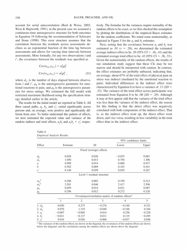
The results for the initial model are reported in Table 6. Allthree causal paths, aj, bj, and c�j , varied significantly acrosspersons and, on average, were positive and significantly dif-ferent from zero. To better understand this pattern of effects,we next estimated the expected value and variance of therandom indirect and total effects, ajbj and ajbj � c�j , respec-

tively. The formulas for the variances require normality of therandom effects to be exact, so we first checked this assumptionby plotting the distributions of the empirical Bayes estimatesfor the random coefficients. We noted some nonnormality, asdepicted in Figure 5 for the aj and bj estimates.

Next, noting that the covariance between aj and bj wasestimated as .01 (r � .26), we determined the estimatedaverage indirect effect to be .29 (95% CI � .16, .41) and theestimated average total effect to be .43 (95% CI � .36, .51).Given the nonnormality of the random effects, the results ofour simulation study suggest that these CIs may be toonarrow and should be interpreted with caution. In contrast,the effect estimates are probably unbiased, indicating that,on average, about 67% of the total effect of physical pain onstress was indirect (mediated by the emotional reaction topain). Individual differences in the indirect effect werecharacterized by Equation 6 to have a variance of .11 (SD �.33). The variance of the total effect across participants wasestimated from Equation 8 to be .08 (SD � .29). Althoughit may at first appear odd that the variance of the total effectwas less than the variance of the indirect effect, the reasonfor this finding is that the direct effect was negativelycorrelated with both components of the indirect effect. Thatis, as the indirect effect went up, the direct effect wentdown, and vice versa, resulting in less variability in the totaleffect than in the indirect effect.

Table 6Empirical Analysis Results

Effect Estimate SE

95% confidence limits

Lower Upper

Fixed (average) effects

dE 0.028 0.026 0.025 0.081dS 1.050 0.013 0.794 1.306a 0.909 0.014 0.880 0.937b 0.302 0.069 0.163 0.441c� 0.148 0.059 0.029 0.267

Level 1 residual structure

�E2 0.206 0.003 0.199 0.212

�S2 2.501 0.046 2.417 2.596

�E 0.059 0.014 0.031 0.087�S 0.296 0.012 0.272 0.320

Covariance/correlation matrix of random effectsa

1 2 3 4 5

1. dEj0.050 0.275 0.276 0.140 0.321

2. dSj0.070 1.319 0.040 0.346 0.104

3. aj 0.007 0.005 0.014 0.258 0.2284. bj 0.011 0.137 0.011 0.119 0.4955. c�j 0.016 0.026 0.006 0.037 0.048a The variances of the random effects are shown on the diagonal, the covariances of the random effects are shownbelow the diagonal, and the correlations among the random effects are shown above the diagonal.


To better understand individual differences in thestrength of the direct, indirect, and total effects, we nextextended the model we have described by adding a Level 2predictor. The predictor of interest was the number of majoracute complications of SCD (ACUTE) the patient reportedhaving experienced within the past year. This predictor wasadded to the equation for each random effect. Of greatestinterest was whether acute complications of SCD wouldmoderate the indirect effect, or ajbj. The coefficient esti-mates indicated that higher levels of acute complicationsreduced the role of emotional reactions to pain as a mediatorbetween physical pain and stress; however, the simulta-neous test of these coefficients was not significant, �2(2) �4.75, p � .093. In contrast, higher levels of acute compli-cations appeared to increase the direct effect of physicalpain on stress, but this was also not significant, t(24.4) �1.82, p � .080.

Given that the moderating effects of ACUTE on the threecausal paths were nonsignificant, the analysis would typi-cally end here. However, simply to demonstrate the meth-odology described in the preceding section, we proceeded toprobe the simple direct, indirect, and total effects of phys-ical pain on stress at each observed count of acute compli-cations, zero through six. As can be seen in Figure 6,although the total effect was relatively unaffected by themoderator, the balance of the direct and indirect effectsshifted markedly. For participants reporting zero acute SCDcomplications in the past year, the effect of physical pain onstress was essentially all indirect. As the number of acuteSCD complications reported by the participant rose, how-ever, this indirect effect diminished to nearly zero, and thedirect effect of physical pain on stress increased to higherlevels. Inferential tests of the simple direct and indirecteffects revealed significant indirect effects for participants

Figure 5. Diagnostic plots for judging the normality assumption for the random slopes involvedin the indirect effect estimate. Top panels are histograms for the empirical Bayes (EB) estimates ofthe random effects obtained by fitting the initial model to the sickle cell disease data; bottom panelsare normal quantile–quantile plots for the EB estimates.


reporting four or fewer acute SCD complications in the pastyear and significant direct effects for participants reportingthree or more complications. The simple total effects wererelatively stable and statistically significant across all ob-served levels of acute SCD complications.

Epistemological Issues in Assessing Mediation

Having established and demonstrated procedures for eval-uating hypotheses of lower level mediation in multilevelmodels, we now review several important epistemologicalissues that must be considered whenever mediation is to beassessed. The foremost assumption of any mediation modelis that the distal predictor and the mediator exert causaleffects on their respective dependent variables. Necessarypreconditions for causal inference are that (a) the variablesinvolved must covary with each other, (b) causes must occurbefore their presumed effects, and (c) sources of spuriouscovariation should be eliminated (Frazier, Tix, & Barron,2004). To satisfy the second condition, X should be mea-sured prior to M and M should be measured prior to Ywhenever possible (Gollob & Reichardt, 1987, 1991). Ex-perimental manipulation of X can greatly strengthen thecausal inference, as can secondary manipulation of M(Spencer, Zanna, & Fong, 2005). With respect to the thirdcondition, MacKinnon et al. (2002) and Holland (1988)noted that the independence assumption made for the cross-equation residuals in Equation 1 is particularly question-able. Violation of this assumption can occur in a number ofways, including the omission of important variables, thepresence of common method variance, and model misspeci-

fication. The result may be bias in the indirect effect esti-mate. Confidence in the independence assumption can beincreased through the inclusion of potential common causesof Y and M (other than X) in the model and through the useof multiple methods of data collection. Further recommen-dations for improving causal inferences can be found inBerk (1988, 2004), Cole and Maxwell (2003), Gollob andReichardt (1987, 1991), and Hoyle and Robinson (2004).

With regard to model specification, one issue that isunique to the lower level mediation model is the partitioningof the covariance structure for the Level 1 observations. Ifthe Level 1 residual covariance structure is not correctlyspecified, then this may lead one to overestimate the vari-ance components for the random effects. As a consequence,one could conclude that there is more heterogeneity in thehypothesized causal effects of the model than is in factpresent in the population of Level 2 units. A second spec-ification issue unique to the multilevel setting is whicheffects should have random versus fixed components. Thisissue is important because misspecification of the randomeffects could also bias the indirect effect estimate. Ideally,the theoretical model of the causal processes will indicatewhich of the causal effects may show heterogeneity acrossLevel 2 units. If, however, theory does not provide strongguidance, then researchers may wish to empirically evaluatethe issue by including random effects for each causal pathand assessing the magnitude of the estimated variance com-ponents for these effects.

In our view, it is rarely the case that an investigator is ableto address all of the aforementioned issues simultaneously.For instance, for the SCD analyses we have presented, the

Figure 6. Bars indicate the decomposition of the average causal effect of physical pain on stressinto a direct effect and an indirect effect through emotional reactions to pain. The total height of eachcolumn conveys the magnitude of the total effect, with the exception of the first column, where thedirect effect is negative and the total effect is indicated with a white horizontal line. Note that thetotal effect of physical pain on stress is relatively constant but that the mediation of this effect byemotional reactions to pain wanes as the severity of sickle cell disease (SCD) increases.


measures are contemporaneous, and questions could beraised about whether the causal effects are in the correctdirection (or bidirectional), whether the estimates are in-flated by common method variance, and whether an autore-gressive structure was sufficient to capture the over-timeresidual correlations. Like the SCD analyses, definitive ev-idence of mediation is often not obtained from a singlemodel; instead, multiple studies are typically necessary.

Limitations and Future Directions

Although we believe that the simultaneous approach wehave proposed to modeling random indirect effects in 1 31 3 1 multilevel mediation models has a number ofstrengths, we would be remiss if we did not also note itslimitations. First, our simulation study considers only asmall set of the possible conditions that might be encoun-tered in practice. Indeed, our own analysis of the SCD datainvolves unbalanced data, potentially nonrandom attrition,and serial dependence, none of which is considered in thesimulation study. We thus view our results as a preliminaryindication of when and where the performance of the pro-posed procedures can be expected to suffer when the as-sumptions of the model are unmet, but more studies areneeded to make more definitive conclusions.

One clear implication of our simulation study is thatadditional thought must be given to the best way to accom-modate nonnormal random effects. One possibility is toretain the current model but implement a nonparametricbootstrap. Recently, Pituch, Stapleton, and Kang (in press)evaluated bootstrapping for conducting tests of mediation inmultilevel models and obtained promising results. Theirresearch was, however, restricted to models with normallydistributed random effects and without random indirecteffects. Unfortunately, the computational burden involvedin bootstrapping the more complex models we consider maybe prohibitive. For instance, the initial model we fitted to theSCD data took 40 min to estimate. Running the same modelon 1,000 resampled data sets would thus take about 28 daysof computing time. Some way must be found to improve theefficiency of the process if bootstrapping is to be a feasibleoption for these models.

An additional limitation of the present approach is that themodel requires that the residuals for the mediator and thedistal outcome be uncorrelated, an assumption that may nothold for reasons discussed in the prior section. For single-level models, one can potentially address this assumption byusing a structural equation model (SEM) in which M and Yare latent variables and the residuals of the indicators for thelatent variables covary across constructs (see, e.g., Bollen,1989, p. 324). SEMs also account for potential measure-ment error in the observed variables and can be used topartial out common method variance (Bollen & Paxton,1998; Kenny & Zautra, 2001). Despite many recent ad-

vances in multilevel structural equation modeling, however,it is currently infeasible to estimate a 13 13 1 mediationmodel with random direct and indirect effects among thelatent variables. The principal difficulty is that the typicalestimators for multilevel SEMs allow for random interceptsbut not random slopes (Bentler & Liang, 2003; Goldstein &MacDonald, 1988; B. O. Muthen, 1994; B. O. Muthen &Satorra, 1995). In principle, maximum likelihood with numer-ical integration (L. K. Muthen & Muthen, 2004) or Bayesianestimation techniques (Ansari, Jedidi, & Dube, 2002) can beused to include random slopes in a multilevel SEM. Futureresearch should explore the potential use of these new methodswith 13 13 1 models for latent variables.

A number of practical difficulties may also be encoun-tered by applied researchers wishing to fit these models.Foremost, in prototypical form, the model includes tworandom intercepts and three random slopes. In general, theestimation of a multilevel model becomes more difficult andcomputationally demanding as the number of random ef-fects increases, and the present case is no exception. Theidentification of the variance components depends heavilyon the number of Level 1 observations per Level 2 unit,whereas the accuracy with which they are estimated de-pends on the number of Level 2 units (Hox, 2002). In oursimulation study, we encountered serious difficulty estimat-ing the model when the number of Level 1 observations wassmall (e.g., four). Given this, certain kinds of study designsare more likely to permit the estimation of this model thanothers. For instance, studies using ecological momentaryassessment (e.g., diary studies) typically yield many observa-tions per unit and hence may be ideally suited for the estima-tion of lower level mediation models. In contrast, studies withfewer observations per unit may not support the estimation offive random effects, forcing the investigator to simplify themodel by removing one or more random effects.

Conclusions

The ability to investigate heterogeneity in causal effects isone of the most attractive features of multilevel models.Most approaches for investigating mediation in multilevelmodels have, however, exclusively focused on fixed causaleffects. In an important next step, Kenny et al. (2003)proposed an approach to evaluating 1 3 1 3 1 mediationwhen the causal paths are random. In this model, the direct,indirect, and total effects vary in strength across the Level 2units of the population. The present article extends the workof Kenny et al. (2003) in two important ways. First, wepresent a simultaneous modeling approach that provides allof the necessary information to calculate the variances ofthe random indirect and total effects as well as the standarderrors of the average indirect and total effects. We believethat the formulas for calculating these standard errors arenew results. Additionally, this simultaneous modeling ap-


proach offers the opportunity to conduct tests of moderatedmediation when the components of the random indirecteffect are predicted by a Level 2 variable. Second, weprovide an initial study of the robustness of the estimatesand CIs for the average indirect effect using simulationmethodology. This study indicates that the estimate of theaverage indirect effect was unbiased under most conditions.The CIs also provided fairly accurate coverage rates whenthe random effects were normal, although they were toonarrow when the random effects were nonnormal. With thiscaveat in mind, we believe that the developments we havepresented offer applied researchers an improved approachfor estimating indirect effects in 1 3 1 3 1 multilevelmediation models. Future developments such as those wehave suggested may offer further improvements, enablingapplied researchers to more fully address hypotheses ofmediation in multilevel data structures.

References

Aiken, L. S., & West, S. G. (1991). Multiple regression: Testingand interpreting interactions. Newbury Park, CA: Sage.

Alwin, D. F., & Hauser, R. M. (1975). The decomposition ofeffects in path analysis. American Sociological Review, 40,37–47.

Ansari, A., Jedidi, K., & Dube, L. (2002). Heterogeneous factoranalysis models: A Bayesian approach. Psychometrika, 67, 49–78.

Baron, R. M., & Kenny, D. A. (1986). The moderator–mediatorvariable distinction in social psychological research: Concep-tual, strategic, and statistical considerations. Journal of Person-ality and Social Psychology, 51, 1173–1182.

Bauer, D. J. (2003). Estimating multilevel linear models as struc-tural equation models. Journal of Educational and BehavioralStatistics, 28, 135–167.

Bauer, D. J., & Curran, P. J. (2005). Probing interactions in fixedand multilevel regression: Inferential and graphical techniques.Multivariate Behavioral Research, 40, 373–400.

Beal, D. J., & Weiss, H. M. (2003). Methods of ecological mo-mentary assessment in organizational research. OrganizationalResearch Methods, 6, 440–464.

Bentler, P. M., & Liang, J. (2003). Two-level mean and covariancestructures: Maximum likelihood via an EM algorithm. In S. P.Reise & N. Duan (Eds.), Multilevel modeling: Methodologicaladvances, issues, and applications (pp. 53–70). Mahwah, NJ: Erl-baum.

Berk, R. A. (1988). Causal inference for sociological data. In N. J.Smelser (Ed.), Handbook of sociology (pp. 155–172). NewburyPark, CA: Sage.

Berk, R. A. (2004). Regression analysis: A constructive critique.Thousand Oaks, CA: Sage.

Bollen, K. A. (1987). Total, direct, and indirect effects in structuralequation models. Sociological Methodology 1987, 17, 37–69.

Bollen, K. A. (1989). Structural equations with latent variables.New York: Wiley.

Bollen, K. A., & Paxton, P. (1998). Detection and determinants ofbias in subjective measures. American Sociological Review, 63,465–478.

Catanzaro, S. J., & Laurent, J. (2004). Perceived family support,negative mood regulation expectancies, coping, and adolescentalcohol use: Evidence of mediation and moderation effects.Addictive Behaviors, 29, 1779–1797.

Cole, D. A., & Maxwell, S. E. (2003). Testing mediational modelswith longitudinal data: Questions and tips in the use of structuralequation modeling. Journal of Abnormal Psychology, 112, 558–577.

Demidenko, E. (2004). Mixed models: Theory and applications.Hoboken, NJ: Wiley.

Frazier, P. A., Tix, A. P., & Barron, K. E. (2004). Testing mod-erator and mediator effects in counseling psychology research.Journal of Counseling Psychology, 51, 115–134.

Gil, K. M., Carson, J. W., Porter, L. S., Ready, J., Valrie, C.,Redding-Lallinger, R., & Daeschner, C. (2003). Daily stress andmood and their association with pain, health-care use and schoolactivity in adolescents with sickle cell disease. Journal of Pe-diatric Psychology, 28, 363–373.

Gil, K. M., Carson, J. W., Porter, L. S., Scipio, C., Bediako, S. M.,& Orringer, E. (2004). Daily mood and stress predict pain,health care use, and work activity in African American adultswith sickle-cell disease. Health Psychology, 23, 267–274.

Goldstein, H. I., & McDonald, R. P. (1988). A general model forthe analysis of multilevel data. Psychometrika, 53, 455–467.

Gollob, H. F., & Reichardt, C. S. (1987). Taking account of timelags in causal models. Child Development, 58, 80–92.

Gollob, H. F., & Reichardt, C. S. (1991). Interpreting and estimat-ing indirect effects assuming time lags really matter. In L. M.Collins & J. L. Horn (Eds.), Best methods for the analysis ofchange (pp. 243–259). Washington, DC: American Psycholog-ical Association.

Goodman, L. A. (1960). On the exact variance of products. Jour-nal of the American Statistical Association, 55, 708–713.

Holland, P. W. (1988). Causal inference, path analysis, and recur-sive structural equations models. Sociological Methodology1988, 18, 449–484.

Hox, J. (2002). Multilevel analysis: Techniques and applications.Mahwah, NJ: Erlbaum.

Hoyle, R. H., & Robinson, J. C. (2004). Mediated and moderatedeffects in social psychological research: Measurement, design,and analysis issues. In C. Sansone, C. C. Morf, & A. T. Panter(Eds.), The Sage handbook of methods in social psychology (pp.213–233). Thousand Oaks, CA: Sage.

James, L. R., & Brett, J. M. (1984). Mediators, moderators, and testsfor mediation. Journal of Applied Psychology, 69, 307–321.

Judd, C. M., & Kenny, D. A. (1981). Process analysis: Estimatingmediation in treatment evaluations. Evaluation Review, 5, 602–619.

Kackar, R. N., & Harville, D. A. (1984). Approximations forstandard errors of estimators of fixed and random effects in


mixed linear models. Journal of the American Statistical Asso-ciation, 79, 853–862.

Kendall, M. G., & Stuart, A. (1969). The advanced theory ofstatistics (3rd ed., Vol. 2). London: Charles Griffen & Co.

Kenny, D. A., Kashy, D. A., & Bolger, N. (1998). Data analysis insocial psychology. In D. Gilbert, S. T. Fiske, & G. Lindzey(Eds.), The handbook of social psychology (4th ed., Vol. 1, pp.223–265). New York: McGraw-Hill.

Kenny, D. A., Korchmaros, J. D., & Bolger, N. (2003). Lowerlevel mediation in multilevel models. Psychological Methods, 8,115–128.

Kenny, D. A., & Zautra, A. (2001). Trait-state models for longi-tudinal data. In L. M. Collins & A. G. Sayer (Eds.), Newmethods for the analysis of change (pp. 243–269). Washington,DC: American Psychological Association.

Kreft, I., & de Leeuw, J. (1998). Introduction to multilevel mod-eling. London: Sage.

Krull, J. L., & MacKinnon, D. P. (1999). Multilevel mediationmodeling in group-based intervention studies. Evaluation Re-view, 23, 418–444.

Krull, J. L., & MacKinnon, D. P. (2001). Multilevel modeling ofindividual and group level mediated effects. Multivariate Be-havioral Research, 36, 249–277.

Lance, C. E. (1988). Residual centering, exploratory and confir-matory moderator analysis, and decomposition of effects in pathmodels containing interactions. Applied Psychological Mea-surement, 12, 163–175.

MacCallum, R. C., Kim, C., Malarkey, W., & Kiecolt-Glaser, J.(1997). Studying multivariate change using multilevel modelsand latent curve models. Multivariate Behavioral Research, 32,215–253.

MacKinnon, D. P., Krull, J. L., & Lockwood, C. M. (2000).Equivalence of the mediation, confounding, and suppressioneffect. Prevention Science, 1, 173–181.

MacKinnon, D. P., Lockwood, C. M., Hoffman, J. M., West, S. G.,& Sheets, V. (2002). A comparison of methods to test mediationand other intervening variable effects. Psychological Methods,7, 83–104.

MacKinnon, D. P., Lockwood, C. M., & Williams, J. (2004).Confidence limits for the indirect effect: Distribution of theproduct and resampling methods. Multivariate Behavioral Re-search, 39, 99–128.

Morgan-Lopez, A. A. (2003). A simulation study of the mediatedbaseline by treatment interaction effect in preventive interven-tion trials. Unpublished doctoral dissertation, Arizona StateUniversity.

Muller, D., Judd, C. M., & Yzerbyt, V. Y. (2005). When moder-ation is mediated and mediation is moderated. Journal of Per-sonality and Social Psychology, 89, 852–863.

Muthen, B. O. (1994). Multilevel covariance structure analysis.Sociological Methods & Research, 22, 376–398.

Muthen, B. O., & Satorra, A. (1995). Complex sample data instructural equation modeling. Sociological Methodology, 1995,216–316.

Muthen, L. K., & Muthen, B. O. (2004). Mplus user’s guide (3rded.). Los Angeles: Muthen & Muthen.

Pituch, K. A., Stapleton, L. M. & Kang, J. Y. (in press). Acomparison of single sample and bootstrap methods to assessmediation in cluster randomized trials. Multivariate BehavioralResearch.

Pituch, K. A., Whittaker, T. A., & Stapleton, L. M. (2005). Acomparison of methods to test for mediation in multisite exper-iments. Multivariate Behavioral Research, 40, 1–24.

Preacher, K. J., Rucker, D. D., & Hayes, A. F. (2006). Suggestedprocedures for addressing moderated mediation hypotheses.Manuscript submitted for publication.

Rao, C. R. (1965). Linear statistical inference and its applications.New York: Wiley.

Raudenbush, S. W., & Bryk, A. S. (2002). Hierarchical linearmodels: Applications and data analysis methods (2nd ed.).Newbury Park, CA: Sage.

Raudenbush, S. W., & Sampson, R. (1999). Assessing direct andindirect effects in multilevel designs with latent variables. So-ciological Methods & Research, 28, 123–153.

Schafer, J. L., & Graham, J. W. (2002). Missing data: Our view ofthe state of the art. Psychological Methods, 7, 147–177.

Schwartz, J. E., & Stone, A. A. (1998). Strategies for analyzingecological momentary assessment data. Health Psychology, 17,6–16.

Shrout, P. E., & Bolger, N. (2002). Mediation in experimental andnonexperimental studies: New procedures and recommenda-tions. Psychological Methods, 7, 422–445.

Spencer, S. J., Zanna, M. P., & Fong, G. T. (2005). Establishing acausal chain: Why experiments are often more effective thanmediational analyses in examining psychological processes.Journal of Personality and Social Psychology, 89, 845–851.

Wegener, D. T., & Fabrigar, L. R. (2000). Analysis and design fornonexperimental data: Addressing causal and noncausal hypoth-eses. In H. T. Reis & C. M. Judd (Eds.), Handbook of researchmethods in social and personality psychology (pp. 412–450).Cambridge, England: Cambridge University Press.

Wei, M., Mallinckrodt, B., Russell, D. W., & Abraham, W. T.(2004). Maladaptive perfectionism as a mediator and moderatorbetween adult attachment and depressive mood. Journal ofCounseling Psychology, 51, 201–212.

West, S. G., & Hepworth, J. T. (1991). Statistical issues in thestudy of temporal data: Daily experiences. Journal of Person-ality, 59, 609–662.

(Appendix follows on next page)


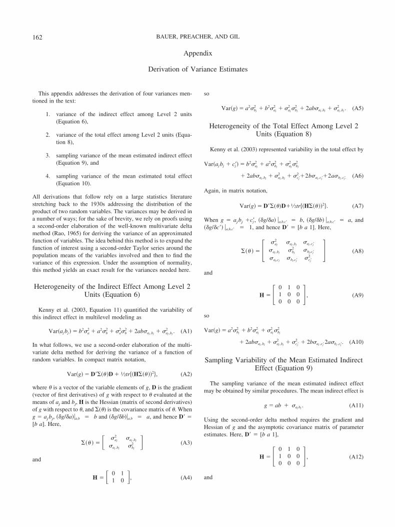
Appendix

Derivation of Variance Estimates

This appendix addresses the derivation of four variances men-tioned in the text:

1. variance of the indirect effect among Level 2 units(Equation 6),

2. variance of the total effect among Level 2 units (Equa-tion 8),

3. sampling variance of the mean estimated indirect effect(Equation 9), and

4. sampling variance of the mean estimated total effect(Equation 10).

All derivations that follow rely on a large statistics literaturestretching back to the 1930s addressing the distribution of theproduct of two random variables. The variances may be derived ina number of ways; for the sake of brevity, we rely on proofs usinga second-order elaboration of the well-known multivariate deltamethod (Rao, 1965) for deriving the variance of an approximatedfunction of variables. The idea behind this method is to expand thefunction of interest using a second-order Taylor series around thepopulation means of the variables involved and then to find thevariance of this expression. Under the assumption of normality,this method yields an exact result for the variances needed here.

Heterogeneity of the Indirect Effect Among Level 2Units (Equation 6)

Kenny et al. (2003, Equation 11) quantified the variability ofthis indirect effect in multilevel modeling as

Var�aj bj � � b2�a2 � a2�b

2 � �a2�b

2 � 2ab�aj ,bj � �aj ,bj

2 . (A1)

In what follows, we use a second-order elaboration of the multi-variate delta method for deriving the variance of a function ofrandom variables. In compact matrix notation,

Var�g� � D��D � 1⁄2tr��H��2�, (A2)

where is a vector of the variable elements of g, D is the gradient(vector of first derivatives) of g with respect to evaluated at themeans of aj and bj, H is the Hessian (matrix of second derivatives)of g with respect to , and () is the covariance matrix of . Wheng � aj bj, �g/a��a,b � b and �g/b��a,b � a, and hence D� �[b a]. Here,

� � � � �aj

2 �aj ,bj

�aj ,bj �bj

2 � (A3)

and

H � � 0 11 0 �, (A4)

so

Var�g� � a2�bj

2 � b2�aj

2 � �aj

2 �bj

2 � 2ab�aj ,bj � �aj ,bj

2 . (A5)

Heterogeneity of the Total Effect Among Level 2Units (Equation 8)

Kenny et al. (2003) represented variability in the total effect by

Var�aj bj � c�j � � b2�aj

2 � a2�bj

2 � �aj

2 �bj

2

� 2ab�aj ,bj � �aj ,bj

2 � �c�j2 �2b�aj ,c�j �2a�bj ,c�j . (A6)

Again, in matrix notation,

Var�g� � D�()D�1⁄2tr��H��2�. (A7)

When g � ajbj �c�j , �g/a� �a,b,c� � b, �g/b� �a,b,c� � a, and�g/c�� a,b,c� � 1, and hence D� � [b a 1]. Here,

� � � � �aj

2 �aj ,bj�aj ,c�j

�aj ,bj �bj

2 �bj,c�j

�aj,cj�bj,c�j �c�j

2 � (A8)

and

H � � 0 1 01 0 00 0 0

� , (A9)

so

Var�g� � a2�bj

2 � b2�aj

2 � �aj

2 �bj

2

� 2ab�aj ,bj � �aj ,bj

2 � �c�j2 � 2b�aj ,c�j 2a�bj ,c�j . (A10)

Sampling Variability of the Mean Estimated IndirectEffect (Equation 9)

The sampling variance of the mean estimated indirect effectmay be obtained by similar procedures. The mean indirect effect is

g � ab � �aj bj . (A11)

Using the second-order delta method requires the gradient andHessian of g and the asymptotic covariance matrix of parameterestimates. Here, D� � [b a 1],

H � � 0 1 01 0 00 0 0

� , (A12)

and


� � � � � a2 � a,b 0

� a,b � b2 0

0 0 ��aj ,bj

2 � (A13)

(asymptotic covariances between fixed and random effect param-eters are zero). Thus,

Var�g� � D�()D � 1⁄2tr��H��2� � b2�a2

� a2�b2

� �a2�b

2� 2ab�a,b� ��a,b�

2 � ��aj ,bj

2 . (A14)

In practice, the sample estimates of these quantities are substitutedfor their population counterparts.

Sampling Variability of the Mean Estimated TotalEffect (Equation 10)

The mean estimated total effect is

g � ab � c� � �aj ,bj . (A15)

Using the second-order delta method requires the gradient andHessian of g and the asymptotic covariance matrix of parameterestimates. Here, D� �[b a 1 1],

H � �0 1 0 01 0 0 00 0 0 00 0 0 0

� , (A16)

and

� � � �� a

2 �a,b �a,c� 0�a,b �b

2�b,c� 0

�a,c� �b,c� �c�2 0

0 0 0 � �aj ,bj

2� . (A17)

Thus,

Var�g� � D��D � 1⁄2tr��H��2�

� b2�a2 � a2�b

2� 2ab�a,b� 2b�a,c� � 2a�b,c�

� ��aj ,bj

2 � �c�2 � �a

2�b2

� ��a,b�2. (A18)

In practice, the sample estimates are substituted for their popula-tion counterparts.

Received March 16, 2005Revision received March 1, 2006

Accepted March 1, 2006 �


Documents

Conceptualizing and Testing Random Indirect Effects … · Conceptualizing and Testing Random Indirect Effects and Moderated ... we would expect their scores on the outcome vari-