Embed Size (px)
Citation preview
Conceptual Linearization of Euler GoverningEquations to Solve High Speed CompressibleFlow Using a Pressure-Based MethodMasoud Darbandi,1 Ehsan Roohi,1 Vahab Mokarizadeh2
1Department of Aerospace Engineering, Sharif University of Technology, Tehran,P.O. Box 11365-8639, Iran
2Energy & Environmental Research Center, Niroo Research Institute, Tehran,P.O. Box 14665-517, Iran
Received 26 February 2006; revision 30 November 2006; accepted 4 May 2007Published online in Wiley InterScience (www.interscience.wiley.com).DOI 10.1002/num.20275
The main objective of the current work is to introduce a new conceptual linearization strategy to improvethe performance of a primitive shock-capturing pressure-based finite-volume method. To avoid a spuriousoscillatory solution in the chosen collocated grids, both the primitive and extended methods utilize twoconvecting and convected momentum expressions at each cell face. The expressions are obtained via aphysical-based discretization of two inclusive statements, which are constructed via a novel incorporation ofthe continuity and momentum governing equations. These two expressions in turn provide a strong couplingamong the Euler conservative statements. Contrary to the primitive work, the linearization in the currentwork respects the definitions and essence of physics behind deriving the Euler governing equations. Theaccuracy and efficiency of the new formulation are then investigated by solving the shock tube as a problemwith moving normal and expansion waves and the converging-diverging nozzle as a problem with strongstationary normal shock. The results show that there is good improvement in performance of the primitivepressure-based shock-capturing method while its superior accuracy is not deteriorated at all. © 2007 WileyPeriodicals, Inc. Numer Methods Partial Differential Eq 00: 000–000, 2007
Keywords: collocated grid; compressible flow; finite volume method; Newton–Raphson linearizationscheme; pressure-based approach; shock-capturing technique
I. INTRODUCTION
The key role of density in high speed flow regimes has resulted in choosing it as a major depen-dent variable in developing numerical algorithms to solve either Euler or Navier–Stokes governingequations. As a preliminary step, the Godunov method was established based on the important roleof density changes in high speed flow regimes [1]. Since the innovation, this primitive method has
Correspondence to: M. Darbandi, Department of Aerospace Engineering, Sharif University of Technology, Tehran,P.O. Box 11365-8639, Iran (e-mail: [email protected])
© 2007 Wiley Periodicals, Inc.
2 DARBANDI, ROOHI, AND MOKARIZADEH
been widely improved from different perspectives including accuracy, conservativity, stability,and consistency, e.g., see Refs. [2–5]. For example, to capture shock more precisely, the primitivemethod has been incorporated with high resolution schemes. Moreover, to reduce the complexityin the high resolution formulations, there have been attempts to compact the computational sten-cil while maintaining the same order of accuracy [6]. Despite such progresses in density-basedmethods, there is major difficulty to solve low Mach number flows efficiently [7–9]. The diffi-culty can be overcome using low Mach number preconditioning, which consequently increasesthe computational cost. Therefore, there has been serious demand to extend new methods capableof solving not only high speed compressible flow but also low Mach number flow with similarefficiencies. In this regard, the pressure-based methods have been practiced to lessen the difficul-ties encountered in solving low Mach flows. As it is known, pressure performs no deficiency insolving low Mach number flow [10–14]. To benefit from this advantage, Rossow [15] developedan alternative method to low speed preconditioning for the computations of nearly incompress-ible flows using a blended pressure/density based method. The evolution of the pressure-basedmethods is described shortly.
From the conservation perspective, the advantages of finite volume method have promotedthe computational fluid dynamics workers to employ it widely. There are two basic choices towrite the finite volume formulation if a pressure-based algorithm is chosen. One choice is thetype of primary dependent variables utilized in the computational algorithm and the other oneis the relative locations of the dependent variables on the computational grids. The primitivefinite-volume work of Patankar and Spalding [16], which is known as SIMPLE, considers thecontinuity equation as a constraint equation for pressure. However, SIMPLE and its variants suf-fer non-physical oscillatory pressure and velocity fields. Staggered grid arrangement has beenemployed as a general remedy to overcome the drawbacks. This arrangement stores the depen-dent variables at two different locations, which are displaced with respect to each other [12, 17].Boundary condition implementation difficulty and excessive book-keeping are two major objec-tions to staggered grid approaches. In addition, the velocities that satisfy mass do not necessarilyconserve momentum in the same control volume. Moreover, more smearing is pronounced arounddiscontinuities [13]. These drawbacks become more crucial in the curvilinear coordinate systemsto solve either laminar [18, 19] or turbulent [20, 21] flow regimes. Therefore, the geometricallysimplicity of the collocated grid arrangement is very attractive and it will be significant if thecause of wavy non-physical pressure field is removed [22].
There are different approaches to suppress the checkerboard problem on a collocated grid. Rhieand Chow [23] used additional momentum-based interpolation to treat the cell face velocities inthe continuity equation. Miller and Schmidt [24] showed that the idea of Ref. [23] would pre-dict spurious cell velocities when local variation of pressure departed considerably from linearity.Askoy and Chen [25] similarly employed momentum weighted interpolation approach to suppressthe checkerboard problem in a finite-analytic scheme. Rahman et al. [26] modified the approachof Ref. [23] by incorporating a non-pressure gradient source term in the face approximations.Date [27] derived a new pressure correction equation, which in turn required a further correctioncalled smoothy pressure correction. Darbandi and Schneider [28] derived both cell face velocitiesvia incorporating the mass and momentum governing equations. Lien [11] adopted the collocatedstorage arrangement for all variables and eliminated the checkerboard oscillations by using apressure-weighted interpolation method, similar to that of Rhie and Chow [23]. As is seen, theabove brief literature review indicates that the dual roles of velocity has been long practiced incollocated schemes. These two velocities can be classified as convected and convecting veloc-ities. They are appropriately substituted in the linearized form of the governing equations. Thesubstitution are normally performed only for the active velocity components in the formulations.
Numerical Methods for Partial Differential Equations DOI 10.1002/num
CONCEPTUAL LINEARIZATION OF EULER EQUATIONS 3
However, the linearization procedure of the governing equations may result in several laggedvelocities, which need to be treated very cautiously.
As it is known, the SIMPLE algorithm was originally developed for solving incompressibleflow. However, there have been major attempts to extend it for compressible flow treatment aswell. Darbandi et al. [12,29–31] have shown that the SIMPLE algorithm can be readily extendedto solve compressible thermobuoyant fields performing high density variation with and withoutemploying the Boussinesq assumption. They have also shown that the extended staggered-basedgrid is capable of solving subsonic Euler flow regimes [14]. In the route of extending incom-pressible flow algorithms to treat high compressible flow regimes, Van Doormal et al. [32] alsoextended SIMPLE and its variants to the solution of compressible flows in the staggered gridcontext. They used a Newton–Raphson linearization strategy [33] to linearize the mass flux in thecontinuity equation. Their linearization scheme considers active role for both density and velocityin the derived formulations. Karki and Patankar [10] provided a pressure-based algorithm usingSIMPLE procedure. They were not able to capture shock precisely in supersonic flow. One ofthe famous variants of SIMPLE is PISO algorithm, which includes one predictor and two cor-rector steps [34]. This algorithm and its variants have been successfully utilized for treating highspeed compressible flow regimes [35, 36]. As was mentioned, Lien [11] developed a pressure-based algorithm on collocated grid incorporating the basic idea of Ref. [23] in his algorithm. vander Heul et al. [13] extended an improved marker-and-cell scheme to treat flow in both com-pressible and incompressible flows. Darbandi and Schneider [28] also developed a fully implicitpressure-based algorithm and solved flow at all speeds on a collocated grid arrangement. Con-trary to Ref. [23], they considered alternative roles for velocity to suppress the spurious solutions.Additionally, they employed the Newton–Raphson linearization strategy to linearize the nonlin-ear convection terms in the momentum equations. Since there are dual roles for the two velocitycomponents in the momentum convection terms, the linearization strategy would be constructedin a manner, which maintains the individual role and conceptual meaning of each velocity in theformulation. This is a key point which has not been taken into account in the preceding collocatedalgorithms.
The major contribution of the current work is to correct the linearization procedure taken ina primitive pressure-based shock-capturing method [37–39] via employing a novel conceptuallinearization, which fully respects the essence of physics behind establishing the flow governingequations. This by itself is a contribution and the new scheme does not necessarily need exhibit-ing a better performance than the primitive method. However, our investigation shows that theefficiency of the extended method is considerably higher than the primitive one while its accu-racy is the same as the primitive one. This outcome can be counted as the second contributionof the current work. To present the achieved outcomes, the extended formulation is evaluatedagainst the primitive one by solving the shock tube and converging-diverging nozzle problems.The accuracy and efficiency of the new algorithm are then compared with those of the primitivework.
II. GOVERNING EQUATIONS
In shock-capturing techniques, it is very customary to present the performance of the newlydeveloped methods by treating the steady quasi-1D and unsteady 1D problems. Similar to manypast investigators, who have chosen either steady flow in converging-diverging nozzle problem[40–42] or unsteady flow in shock tube problem [5, 13, 43], we choose the unsteady quasi-1Dgoverning equations to quantify the performance of our proposed linearization. We have targeted
Numerical Methods for Partial Differential Equations DOI 10.1002/num
4 DARBANDI, ROOHI, AND MOKARIZADEH
both the steady quasi-1D flow and the unsteady Riemann problems in our study. The unsteadyquasi-one-dimensional form of the Euler governing equations is written as
∂q∂τ
+ ∂B(q)
∂x= s (2.1)
where the solution vector q, the convection flux vector B(q), and the source term vector s arerespectively given by
q = (ρA, ρuA, ρeA)T (2.2)
B = (ρuA, ρu2A, ρueA + puA)T (2.3)
s = (0, −A(∂p/∂x), 0)T (2.4)
In the earlier equations, τ , ρ, p, u, and A represent time, density, pressure, velocity, and thecross-section area, respectively. If we neglect the change in potential energy, the total energy perunit mass for a perfect gas is given by e = cvt +u2/2, where t is temperature and cv is the specificheat value at constant volume. Considering this expression, the equation of state p = ρRt relatesthe velocity and pressure fields to the temperature field in compressible flows. The discretizedgoverning equations are simultaneously solved for pressure p, temperature t , and momentumcomponent f (≡ ρu) variables of which the latter one is chosen instead of the velocity variable.Past experience has shown that the use of momentum component as a dependent variable canresult in several important outcomes in a pressure-based shock-capturing method. For example,it provides a strong analogy between the compressible and incompressible governing equations.This in turn enables the solution of compressible flow using incompressible methods [12, 37]. Itsimplifies the required linearization procedure [38]. It suppresses the oscillations occurred pass-ing through a discontinuity [44]. It can also improves the performance of the pressure-basedshock-capturing methods [39].
III. DOMAIN DISCRETIZATION
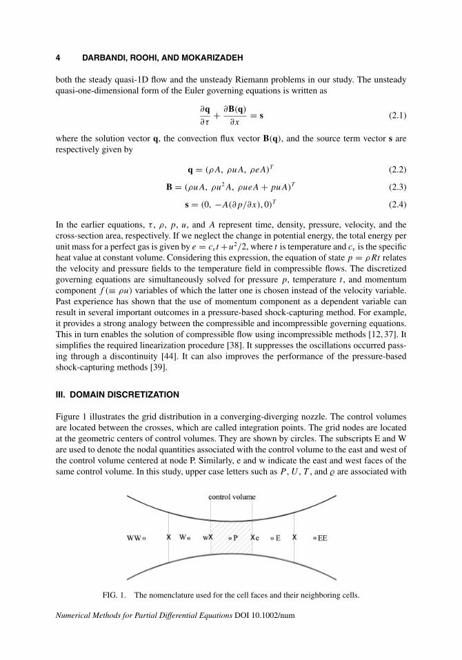
Figure 1 illustrates the grid distribution in a converging-diverging nozzle. The control volumesare located between the crosses, which are called integration points. The grid nodes are locatedat the geometric centers of control volumes. They are shown by circles. The subscripts E and Ware used to denote the nodal quantities associated with the control volume to the east and west ofthe control volume centered at node P. Similarly, e and w indicate the east and west faces of thesame control volume. In this study, upper case letters such as P , U , T , and � are associated with
FIG. 1. The nomenclature used for the cell faces and their neighboring cells.
Numerical Methods for Partial Differential Equations DOI 10.1002/num
CONCEPTUAL LINEARIZATION OF EULER EQUATIONS 5
quantities at main nodes, while lower case letters such as p, u, t , and ρ refer to quantities at thecell faces (or integration points).
IV. COMPUTATIONAL MODELLING
Equation (2.1) can be integrated over an arbitrary control volume, see the shaded volume in Fig. 1.Using the divergence theorem, integration of the continuity equation yields
∫∫A
∂(ρA)
∂τdA +
∫S
(ρuA)dS = 0 (4.1)
where S indicates the integration over the cell faces. Since the current method is fully implicit,the second term is evaluated at the advanced time and the transient term is approximated using amass-lumped approach. The latter treatment yields
∫∫A
∂(ρA)
∂τdA ≈ �x
(�P − �o
P)
�τAP (4.2)
where �o
Pindicates the lumped density of the cell centered at P and its magnitude is obtained
from the preceding time step. The second term in Eq. (4.1) is simply integrated over the boundaryof the cell. It results in ∫
S
(ρuA)dS ≈ (ρuA)e − (ρuA)w (4.3)
Eventually, the discretized form of the mass equation can be written as
�x(�P − �oP)
�τ+ je(ρu)e − jw(ρu)w = 0 (4.4)
The parameters je = Ae/AP and jw = Aw/AP represent the ratios of the east and west cell faceareas respectively to the area at the cell center. Since density is considered as a secondary unknownin our pressure-based algorithm, the transient term in Eq. (4.4) needs to be linearized further. Asimple linearization idea is suggested as � = (1/RT )P , which considers an active role for P anda passive role for T . Alternatively, we may employ a Taylor series of that to consider active rolesfor both P and T , i.e.,
� ≈ � + ∂�
∂P(P − P ) + ∂�
∂T(T − T ) (4.5)
where
∂�
∂P= 1
RT
∂�
∂T= − P
RT 2(4.6)
The integration of the momentum equation over the chosen control volume yields∫∫
A
∂(ρuA)
∂τdA +
∫S
(ρu2A) dS +∫∫
A
[∂(pA)
∂x− p
∂A
∂x
]dA = 0 (4.7)
The use of a mass-lumped approach for the transient term results in∫∫
A
∂(ρuA)
∂τdA ≈ �x[(�U)P − (�U)o
P ]�τ
AP (4.8)
Numerical Methods for Partial Differential Equations DOI 10.1002/num
6 DARBANDI, ROOHI, AND MOKARIZADEH
Additionally, the integration of the momentum convection term over the cell faces yields
∫S
(ρu2A) dS ≈ (ρu2A)e − (ρu2A)w (4.9)
The last term in Eq. (4.7) can be approximated by
∫∫A
[∂(pA)
∂x− p
∂A
∂x
]dA ≈ (pA)e − (pA)w − Pp(Ae − Aw) (4.10)
Eventually, the discretized form of the momentum equation can be presented by
� x[(�U)P − (�U)oP]
�τ+ jeue(ρu)e − jwuw(ρu)w + je pe − jw pw − PP(je − jw) = 0 (4.11)
To be able to use a linear algebraic solver in our fully implicit algorithm, the nonlinear con-vection terms in Eq. (4.11) need to be linearized properly. Assuming the momentum componentρu as a primary dependent variable, a simple linearization scheme suggests
ρuu ≈ u(ρu) (4.12)
However, a more sophisticated linearization, which considers the active impact of the two vari-ables, is obtained using the Newton–Raphson Linearization Scheme, NRLS [33]. The use ofNRLS results in
u(ρu) ≈ u(ρu) + (ρu)u − ρuu (4.13)
If NRLS is further applied to u = ρu/ρ in the second term on the RHS, Eq. (4.13) becomes
ρuu ≈ 2u(ρu) − u2ρ (4.14)
A general expression to include both Eqs. (4.12) and (4.14) can be defined as
ρuu ≈ 2k1u(ρu) − k2u2ρ (4.15)
where k1 and k2 are two constants. If k1 = k2 = 1, it results in NRLS, i.e., Eq. (4.14). On the otherhand, if k1 = 1/2 and k2 = 0, it yields a simple linearization, i.e., Eq. (4.12). Equation (4.14)has been tested in 1D investigation with success [38, 45]. The experience has shown that NRLSwould generally perform better than the simple linearization scheme.
The next step is to treat the energy equation. This equation involves more nonlinear terms thanthe preceding equations. The energy equation can be similarly integrated over the chosen controlvolume. It yields ∫∫
A
∂(ρeA)
∂τdA +
∫S
A(ρue + pu) dS = 0 (4.16)
Similar to the mass and momentum equations, the integrals can be treated properly. Theconservable form can be eventually written as
� x[(� E)P − (� E)oP]
�τ+ (ρuej)e − (ρuej)w + (puj)e − (puj)w = 0 (4.17)
Numerical Methods for Partial Differential Equations DOI 10.1002/num
CONCEPTUAL LINEARIZATION OF EULER EQUATIONS 7
The nonlinear �E in the transient term can be linearized with respect to � and E using NRLS.On the other hand, the internal energy variable E can be linearized to E = cvT + (U/2�)(�U).Our experience shows that these linearizations provide more robust convergence. Using theselinearization strategies, the transient term in Eq. (4.17) is approximated by
� x[(� E)P − (� E)oP]
�τ≈ �x
�τ
[U
2(�U) + E
RTP +
(�cv − (�E)
T
)T − (�E)o
]P
(4.18)
Similarly, using NRLS for ρue term, linearizing it with respect to e and ρu, and utilizing thelinearized form suggested for E (or e) finally yield
ρue ≈(
e + u2
2
)f + (cvf )t − (ef ) (4.19)
The two last terms in the LHS of Eq. (4.17) can be converted to Rtf . This can be achieved via theequation of state. Additionally, Rtf can be linearized with respect to f and t using either simplelinearization or NRLS. The latter choice results in
up = Rtf ≈ (cp − cv)(tf − f t) − Rf t (4.20)
The combination of Eqs. (4.19) and (4.20) is given by
ρue + up ≈ (cp t + u2)f + (cpf )t − (e + Rt)f (4.21)
The substitutions of Eqs. (4.18) and (4.21) in Eq. (4.17), the discretized energy equation is writtenas
�x
�τ
[U
2(�U) + E
RTP +
(�cv − (�E)
T
)T − (�E)o
]P
+[(cp t + u2)f + (cpf )t − (e + Rt)f ]je
− {[(cp t + u2)f + (cpf )t − (e + Rt)f ]j}w = 0 (4.22)
By this derivation, the discretization of the Euler governing equation is finished. The next step isto approximate the magnitudes at cell faces in terms of the magnitudes at the nodes. At this stage,it is worth to mention that there are many different choices to linearize the nonlinear terms in theconservative statements. However, our main objective in this work is not to examine the impactof different possible linearizations but to extend our conceptual linearization, which is applicableto nonlinear convection terms in the momentum equations, see Section C.
A. Integration Point Equations
To make the algebraic system of equations well-posed, this stage of our modelling requires topresent the major dependent variables at cell faces in terms of nodal variables, see f (or ρu) inEq. (4.4), p in Eq. (4.11), and t in Eq. (4.22). Therefore, it is necessary to derive suitable expres-sions for momentum component, pressure, and temperature at the cell faces. Upwind, QUICK, andHYBRID schemes can be nominated as suitable mathematical interpolations [17]. Alternatively,there are more advanced schemes, which include more physics of flow. For example, Prakash andPatankar [46] presented profiles which were attempting to include the relevant physics into theinterpolation functions. Schneider and Raw [47] employed Physical Influence Scheme PIS, which
Numerical Methods for Partial Differential Equations DOI 10.1002/num
8 DARBANDI, ROOHI, AND MOKARIZADEH
considered the flow governing equations, to derive the integration point expressions in incom-pressible flow simulations. Darbandi and Schneider [28,37] extended this model to compressibleflow simulations. The fundamental concepts of PIS will be employed in this work as well.
The expressions for the momentum components can be derived from the momentum equation.In this regard, the momentum equation given in Eq. (2.1) is expanded to
A∂f
∂τ+ u
∂(f A)
∂x+ f A
∂u
∂x+ A
∂p
∂x= 0 (4.23)
The terms in this equation are differenced in certain manners, which respect the correct physicsof flow. To achieve this purpose, they are approximated by
A∂f
∂τ
∣∣∣∣e
≈ Aefe − f o
e
�τ(4.24)
u∂(f A)
∂x
∣∣∣∣e
≈ ue(Af )e − (AF)P
�x/2(4.25)
f A∂u
∂x
∣∣∣∣e
≈ f eAe(fe/ρe − FP/�P)
�x/2(4.26)
A∂p
∂x
∣∣∣∣e
≈ AePE − PP
�x(4.27)
Consistent with their physics, the convection terms are treated in an upwind manner. Anotherpossible form for Eq. (4.26) is f A∂u/∂x ≈ A∂u/∂x f . However, this scheme resulted in poorconvergence of the method. The substitutions of the discretized terms into Eq. (4.23) and itsrearrangement finally result in an expression for the momentum component at integration point.A compact form of that can be written as
fe = 2Ce(AP/Ae + ρe/�P)
1 + 4CeFP + Ce
ue(1 + 4Ce)(PP − PE) + f o
e
1 + 4Ce(4.28)
where the Courant number is defined as C = u�t/�x. Equation (4.28) indicates that the use of aphysical influence scheme produces a strong connection between the integration point variable atface e and its neighboring nodal variables located at P and E. It can be shown that the substitutionsof fe and fw in the mass Eq. (4.4) and momentum Eq. (4.11) equations provide reliable couplingbetween pressure and velocity fields.
The expression for the temperature at integration point can be obtained by suitable discretizationof the energy equation given by Eq. (2.1). This equation is rewritten as
ρcv∂t
∂τ+ ρucv
∂t
∂x+ p
∂u
∂x+ pu
∂[ln(A)]∂x
= 0 (4.29)
The transient term is discretized similar to Eq. (4.24). The upwind and central differences areutilized for the second and third terms, respectively. The last term is treated as a source term.
Numerical Methods for Partial Differential Equations DOI 10.1002/num
CONCEPTUAL LINEARIZATION OF EULER EQUATIONS 9
These considerations yield
ρcv∂t
∂τ
∣∣∣∣e
≈ ρecvte − to
e
�τ(4.30)
ρucv∂t
∂x
∣∣∣∣e
≈ fecvte − TP
�x/2(4.31)
p∂u
∂x
∣∣∣∣e
≈ peUE − UP
�x(4.32)
pu∂[ln(A)]
∂x
∣∣∣∣e
≈ peue∂[ln(A)]
∂x
∣∣∣∣e
(4.33)
Using the earlier approximations, the temperature expression at integration point is obtainedfrom
te ≈ 2Ce
(1 + 2Ce)Tp + Cepe
(ρu)ecv(1 + 2Ce)
(FP
�P− FE
�E
)
− �xCepe
ρecv(1 + 2Ce)
∂[ln(A)]∂x
∣∣∣∣e
+ toe
(1 + 2Ce)(4.34)
Furthermore, the unknown density at integration points can be calculated from the equationof state. In this regard, the equation of state can be firstly linearized with respect to pressure andtemperature using Eq. (4.5). Secondly, the pressure (see the next paragraph) and temperature,Eq. (4.34), expressions are substituted in that.
Schneider and Raw [47] used the pressure Poisson equation as an explicit equation and showedthat the pressure field would be strongly elliptic in incompressible flow. Similarly, we use a linearinterpolation to determine the pressure variable at integration points, i.e., pe ≈ (PP + PE)/2, ifthe local flow is subsonic. However, if the flow is supersonic we utilize an upwind scheme toapproximate the pressure at the cell faces.
B. Checkerboard Problem and Remedy
In the preceding section, we obtained f , p, t , and ρ expressions at the cell faces. The substitutionof these expressions in Eqs. (4.4, 4.11, 4.22) eliminates the unknowns at the cell faces in ourderivations. However, it is necessary to investigate the checkerboard problem in our extendedcollocated formulation. Darbandi and Bostandoost [44] launched their incompressible investiga-tion and showed that the substitution of the derived momentum expression, Eq. (4.28), in bothmass Eq. (4.4) and momentum Eq. (4.11) equations might produce unrealistic wavy pressure andmomentum solutions. Unfortunately, the spurious solutions fully satisfy the governing equationsand their imposed boundary conditions. This instability in the solution is similarly reported byother finite-volume pressure-based investigators [22]. To suppress such non-physical zigzag solu-tions, they suggest and employ a new statement to derive the second expression for the momentumcomponent at the integration point. Their primary purpose has been to include the role of continuityequation in deriving the second momentum component expression. Thus, the second expressionshould be obtained in a manner, which takes into account the roles of not only the mass but alsothe momentum governing equations. To achieve their purpose, they suggested
[(Momentum Eq. Error) − u(Mass Eq. Error)] = 0 (4.35)
Numerical Methods for Partial Differential Equations DOI 10.1002/num
10 DARBANDI, ROOHI, AND MOKARIZADEH
As is seen, this suggestion takes into account the effect of both continuity and momentum equationerrors in the new expression. The justification behind defining and using this special form is toprovide an inclusive statement, very similar to Eq. (4.28), to approximate our second momentumcomponents at the cell faces. To achieve this, we need starting from the basic governing equations,very similar to the one given by Eq. (4.23). In this regard, we suggest a new relation, which ismore meaningful for the compressible flow applications. The new relation is defined as
[A
∂f
∂τ+ u
∂(f A)
∂x+ f A
∂u
∂x+ A
∂p
∂x
]− u
[A
∂ρ
∂τ+ ∂(f A)
∂x
]= 0 (4.36)
The above statement indicates that two types of errors are incorporated in extending the secondcell-face expression. In fact, if a nonexact solution is substituted into the mass and momentumequations, it will result in errors or residuals for both of them. Additionally, if the nonexact solutiondoes not satisfy only the mass equation, the impact is subsequently appeared in the second cellface expression but not the first one. The discretization of the first brackets in Eq. (4.36) is exactlysimilar to what was fulfilled for the momentum integration point equation, see Eqs. (4.24)–(4.27).However, the terms in the second brackets are approximated using
uA∂ρ
∂τ
∣∣∣∣e
≈ ueAe∂ρ
∂τ
∣∣∣∣e
(4.37)
u∂(f A)
∂x
∣∣∣∣e
≈ ueAe fe − AP FP
�x/2(4.38)
The substitutions of Eqs. (4.24)–(4.27) and Eqs. (4.37)–(4.38) in Eq. (4.36) and its suitablerearrangement finally yield
fe = 2Ce
1 + 2Ce
ρe
�P
Fp + Ce
1 + 2Ce(PP − PE) + f o
e
1 + 2Ce+ Ce�x
1 + 2Ce
∂ρ
∂τ
∣∣∣∣e
(4.39)
We call this new expression convecting momentum and refer to the preceding expression givenin Eq. (4.28) as convected momentum. We have labelled the convecting momentum with a hatto distinguish it from the convected one. The substitution of the convecting momentum into thecontinuity equation Eq. (4.4) entirely suppresses the possibility of a zigzag pressure field in thedomain [44]. Moreover, Eq. (4.4) is used to solve the pressure field now. In another words, althoughthe continuity equation in its original form has no trace of active pressure variable, the substitutionof Eq. (4.39) in Eq. (4.4) permits to solve Eq. (4.4) for the pressure field now.
C. Conceptual Linearization Strategy
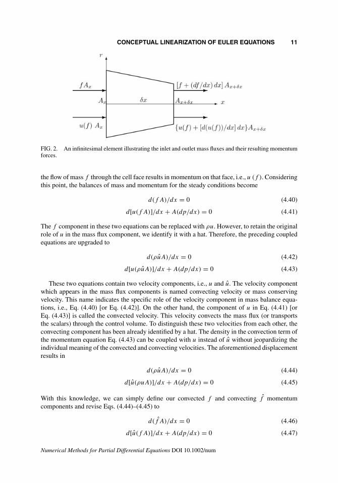
Figure 2 shows an infinitesimal volume with a finite length of δx taken from Fig. 1. The inletand outlet mass flow rates in addition to their resulting momentum forces are indicated at theleft and right faces of the element. Since we are concerned on the role of mass flux, we avoidpresenting the pressure forces around this volume. To emphasize the critical role of momentumcomponent in the continuity equation (and subsequently in our formulations), we have used massflux component f instead of the multiplication of ρ and u, i.e., ρu, in this figure. As it is known,
Numerical Methods for Partial Differential Equations DOI 10.1002/num
CONCEPTUAL LINEARIZATION OF EULER EQUATIONS 11
FIG. 2. An infinitesimal element illustrating the inlet and outlet mass fluxes and their resulting momentumforces.
the flow of mass f through the cell face results in momentum on that face, i.e., u (f ). Consideringthis point, the balances of mass and momentum for the steady conditions become
d(f A)/dx = 0 (4.40)
d[u(f A)]/dx + A(dp/dx) = 0 (4.41)
The f component in these two equations can be replaced with ρu. However, to retain the originalrole of u in the mass flux component, we identify it with a hat. Therefore, the preceding coupledequations are upgraded to
d(ρuA)/dx = 0 (4.42)
d[u(ρuA)]/dx + A(dp/dx) = 0 (4.43)
These two equations contain two velocity components, i.e., u and u. The velocity componentwhich appears in the mass flux components is named convecting velocity or mass conservingvelocity. This name indicates the specific role of the velocity component in mass balance equa-tions, i.e., Eq. (4.40) [or Eq. (4.42)]. On the other hand, the component of u in Eq. (4.41) [orEq. (4.43)] is called the convected velocity. This velocity convects the mass flux (or transportsthe scalars) through the control volume. To distinguish these two velocities from each other, theconvecting component has been already identified by a hat. The density in the convection term ofthe momentum equation Eq. (4.43) can be coupled with u instead of u without jeopardizing theindividual meaning of the convected and convecting velocities. The aforementioned displacementresults in
d(ρuA)/dx = 0 (4.44)
d[u(ρuA)]/dx + A(dp/dx) = 0 (4.45)
With this knowledge, we can simply define our convected f and convecting f momentumcomponents and revise Eqs. (4.44)–(4.45) to
d(f A)/dx = 0 (4.46)
d[u(f A)]/dx + A(dp/dx) = 0 (4.47)
Numerical Methods for Partial Differential Equations DOI 10.1002/num
12 DARBANDI, ROOHI, AND MOKARIZADEH
It is worth to note that an arbitrary switch from the convected component to convecting one orvice versa may jeopardize the original concepts on which the governing equations are founded.Additionally, as was mentioned before, the past researchers have shown that the use of two differ-ent velocities in the continuity and momentum equations has the advantages of suppressing thepossible pressure-velocity decoupling phenomenon in collocated solution domains [23].
Considering the above physical-based definitions, there are two major choices to linearize theconvection term in the momentum equation Eq. (4.11) with respect to the momentum component.A simple linearization choice for the convection terms of the momentum equation permits anactive role only for the convected momentum component. This linearization scheme results in
uf ≈ ¯uf (4.48)
A second linearization choice is to employ a Newton–Raphson Linearization Scheme (NRLS).This scheme considers more active role for the individual components in the nonlinear term. Backto Eq. (4.13), the convection term in Eq. (4.47) can be linearized to
u(f A) ≈ ( ¯uA)f + (f A)u − uf A (4.49)
Since u is not a major unknown in this study, we use NRLS and linearize the convecting velocitycomponent shown in the second term on the LHS in terms of (ρu), i.e.,
u = (ρu)
ρ≈ 1
ρ(ρu) −
¯uρ
ρ + ¯u (4.50)
The substitution of Eq. (4.50) in Eq. (4.49) and performing some more simplifications finallyresult in
uf ≈ ¯u(f ) + u(f ) − uuρ (4.51)
This linearization scheme considers active roles for both convected and convecting momentumcomponents as well as density in the convection term in Eq. (4.11). The density term may besimply lagged and replaced with the known density of the previous iteration. We leave it in therest of our formulations as it is. Considering the two definitions of the momentum components,we present a general expression which includes both the simple Eq. (4.48) and NRLS Eq. (4.51)cases. The general form is suggested as
uf ≈ ¯uf + k′(uf − uuρ) (4.52)
where k′ = 0 results in a simple linearization, i.e., Eq. (4.48), and k′ = 1 represents NRLS,i.e., Eq. (4.51). If we ignore the individual concepts involved in the convected and convectingcomponents, it yields u = u and f = f . Then, Eq. (4.52) can be replaced with a new one givenby
(ρu u = ρuu) ≈ [(2k1 uf − k2 u2ρ) = (2k1¯uf − k2
¯u2ρ)] (4.53)
where k1 and k2 are two constants, which make the two linearizations possible. Equation (4.53)is identical with Eq. (4.15), which was derived without the knowledge of convecting and con-vected components. Similar to Eq. (4.15), the consideration of k1 = k2 = 1 results in NRLS,i.e., Eq. (4.14), and the consideration of k1 = 1
2 and k2 = 0 results in a simple linearization, i.e.,Eq. (4.12).
Numerical Methods for Partial Differential Equations DOI 10.1002/num
CONCEPTUAL LINEARIZATION OF EULER EQUATIONS 13
In the following section, we evaluate the performance of our new developed linearizations insolving unsteady and steady flows using either Eq. (4.53) as Simple Newton–Raphson Lineariza-tion Scheme (SNRL) or Eq. (4.52) as Improved Newton–Raphson Linearization Scheme (INRL)to linearize the convection terms in the momentum equations, i.e., Eq. (4.11).
V. RESULTS AND DISCUSSION
In this section, the conceptual linearization is applied to solve both steady and unsteady flowswith shock. In this regard, the converging-diverging nozzle and shock tube problems are chosento evaluate the extended formulations. The nozzle problem is known as a standard test case toexamine the performance of steady shock-capturing techniques in solving a solution domain witha wide range of Mach numbers including a strong normal shock. Alternatively, the shock tubeproblem is known as a standard test case to evaluate the unsteady shock-capturing techniques.Both the transient flow features (i.e., moving normal shock and expansion waves as well as acontact discontinuity) and a wide range of flow Mach numbers (i.e., subsonic, transonic, andsupersonic regimes) can be targeted in the latter case. To stop the iterations in each time step, theconvergence criterion ε at each time step is checked using
max(|(Pi − Pi)/Pi |, |(Ti − Ti)/Ti |) ≤ (ε = 10−10) (5.1)
where the subscript i represents the node number. The gas properties are cv = 720 J/KgK,R = 287.0 J/KgK, and γ = 1.4.
A. The Accuracy of the Extended Scheme
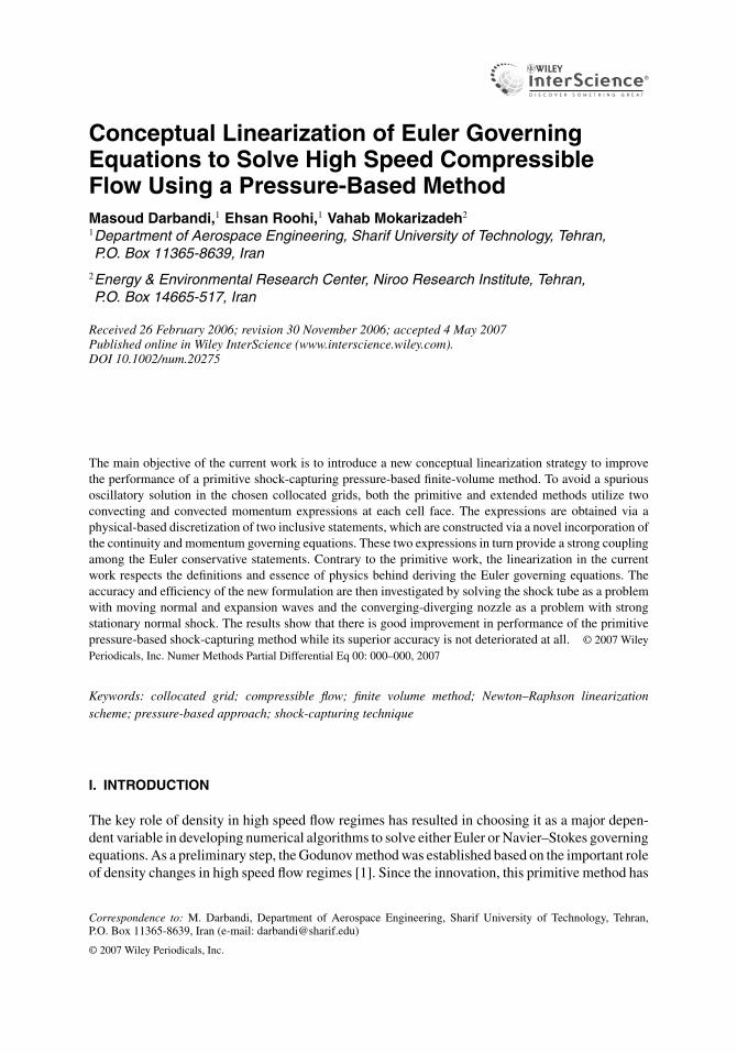
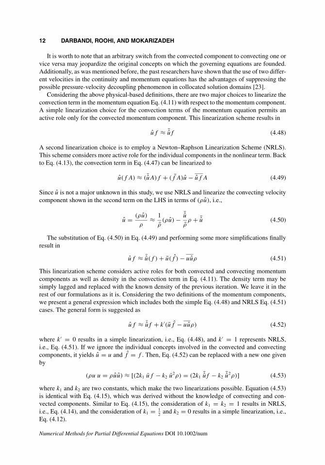
At the first stage, we examine the unsteady shock tube problem. The shock tube length is 1 m anda total of 201 nodes is uniformly distributed along it. The air pressures are 1,000 and 100 KPain the high and low-pressure sides, respectively. The initial temperature is 25◦C in both sides.Following Refs. [38, 45], the results are normally presented at 500 µs after rupturing the sep-arating diaphragm. Figure 3 illustrates the distributions of density, pressure, temperature, andMach number using a Courant number of 0.286. The density, pressure, and temperature are non-dimensionalized using their respective values in the lower pressure side. The figure presents the
FIG. 3. The numerical solutions in the shock tube problem using both SNRL and INRL schemes and theircomparisons with the exact solutions.
Numerical Methods for Partial Differential Equations DOI 10.1002/num
14 DARBANDI, ROOHI, AND MOKARIZADEH
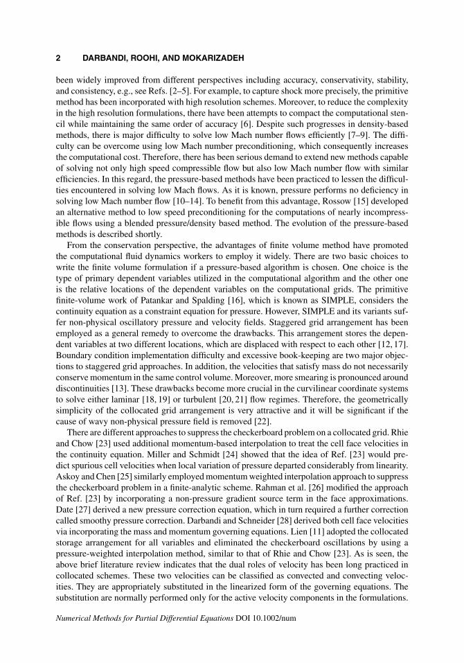
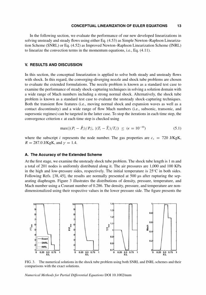
FIG. 4. A comparison of the present solution with that of van der Heul et al. [13].
results of both INRL and SNRL schemes. They are compared with each other and those of ana-lytical solutions. The results of both INRL and SNRL schemes are in good agreement with theanalytical solutions. Additionally, the two INRL and SNRL schemes perform similar accuracies.In another words, the numerical solutions are independent of the selected linearization scheme.This conclusion was definitely predictable because the final results of the two schemes should notbe significantly affected by the choice of scheme to treat the nonlinear convection terms in themomentum equations.
Although it is not a main concern in this work, our study shows that the accuracy achievedin this unsteady solution is comparable and even better than the accuracies presented by a fewother Euler flow solvers. For example, comparing the current results with those of the primitiveGodunov method [1], the artificially upstream flux vector splitting of Sun and Takayama [48], anddifferent weighted essentially nonoscillatory schemes of Titarev and Toro [49], the accuracy ofthe current solution is excellent. It should be noted that the current accuracy is obtained withoutenforcing any additional filters and/or features. Since it is more rational to compare our resultswith those of pressure-based methods, Fig. 4 presents the current Mach distribution and comparesit with that of van der Heul et al. [13], who benefit from the advantages of a pressure-correctionmethod. They solve Sod’s Riemann problem using a few different schemes of which we havechosen the one, which is more consistent with our formulation and its discretization. The Sod’sRiemann problem is solved in similar conditions for both cases.
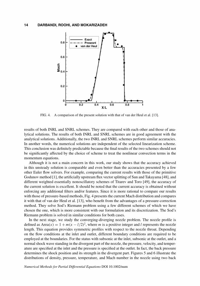
In the next stage, we study the converging-diverging nozzle problem. The nozzle profile isdefined as Area(x) = 1 + m(x − l/2)2, where m is a positive integer and l represents the nozzlelength. This equation provides symmetric profiles with respect to the nozzle throat. Dependingon the flow conditions at the inlet and outlet, different boundary conditions are required to beemployed at the boundaries. For the status with subsonic at the inlet, subsonic at the outlet, and anormal shock wave standing in the divergent part of the nozzle, the pressure, velocity, and temper-ature are specified at the inlet and the pressure is specified at the outlet. In fact, the back pressuredetermines the shock position and its strength in the divergent part. Figures 5 and 6 illustrate thedistributions of density, pressure, temperature, and Mach number in the nozzle using two back
Numerical Methods for Partial Differential Equations DOI 10.1002/num
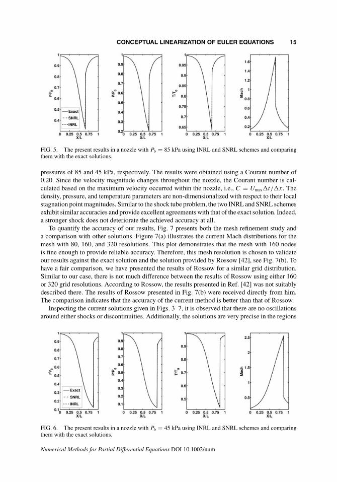
CONCEPTUAL LINEARIZATION OF EULER EQUATIONS 15
FIG. 5. The present results in a nozzle with Pb = 85 kPa using INRL and SNRL schemes and comparingthem with the exact solutions.
pressures of 85 and 45 kPa, respectively. The results were obtained using a Courant number of0.20. Since the velocity magnitude changes throughout the nozzle, the Courant number is cal-culated based on the maximum velocity occurred within the nozzle, i.e., C = Umax�t/�x. Thedensity, pressure, and temperature parameters are non-dimensionalized with respect to their localstagnation point magnitudes. Similar to the shock tube problem, the two INRL and SNRL schemesexhibit similar accuracies and provide excellent agreements with that of the exact solution. Indeed,a stronger shock does not deteriorate the achieved accuracy at all.
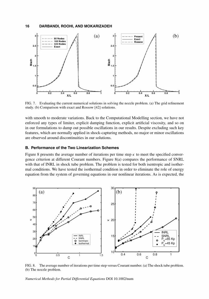
To quantify the accuracy of our results, Fig. 7 presents both the mesh refinement study anda comparison with other solutions. Figure 7(a) illustrates the current Mach distributions for themesh with 80, 160, and 320 resolutions. This plot demonstrates that the mesh with 160 nodesis fine enough to provide reliable accuracy. Therefore, this mesh resolution is chosen to validateour results against the exact solution and the solution provided by Rossow [42], see Fig. 7(b). Tohave a fair comparison, we have presented the results of Rossow for a similar grid distribution.Similar to our case, there is not much difference between the results of Rossow using either 160or 320 grid resolutions. According to Rossow, the results presented in Ref. [42] was not suitablydescribed there. The results of Rossow presented in Fig. 7(b) were received directly from him.The comparison indicates that the accuracy of the current method is better than that of Rossow.
Inspecting the current solutions given in Figs. 3–7, it is observed that there are no oscillationsaround either shocks or discontinuities. Additionally, the solutions are very precise in the regions
FIG. 6. The present results in a nozzle with Pb = 45 kPa using INRL and SNRL schemes and comparingthem with the exact solutions.
Numerical Methods for Partial Differential Equations DOI 10.1002/num
16 DARBANDI, ROOHI, AND MOKARIZADEH
FIG. 7. Evaluating the current numerical solutions in solving the nozzle problem. (a) The grid refinementstudy. (b) Comparison with exact and Rossow [42] solutions.
with smooth to moderate variations. Back to the Computational Modelling section, we have notenforced any types of limiter, explicit damping function, explicit artificial viscosity, and so onin our formulations to damp out possible oscillations in our results. Despite excluding such keyfeatures, which are normally applied in shock-capturing methods, no major or minor oscillationsare observed around discontinuities in our solutions.
B. Performance of the Two Linearization Schemes
Figure 8 presents the average number of iterations per time step κ to meet the specified conver-gence criterion at different Courant numbers. Figure 8(a) compares the performance of SNRLwith that of INRL in shock tube problem. The problem is tested for both isentropic and isother-mal conditions. We have tested the isothermal condition in order to eliminate the role of energyequation from the system of governing equations in our nonlinear iterations. As is expected, the
FIG. 8. The average number of iterations per time step versus Courant number. (a) The shock tube problem.(b) The nozzle problem.
Numerical Methods for Partial Differential Equations DOI 10.1002/num
CONCEPTUAL LINEARIZATION OF EULER EQUATIONS 17
average number of iterations per time step normally increases as Courant increases. Our experi-ence showed that the number of iterations at earlier time steps would be much higher than the nextones. Additionally, the number of iterations may reduce to as low as 3–5 iterations per time step inCourant numbers less than 0.5 if time has elapsed enough. Irrespective of the type of two schemes,their performances show considerable difference as Courant increases. However, the differencesdiminish at lower Courant numbers. A careful comparison indicates that the choice of isothermalcase results in a higher number of iterations with respect to the corresponding isentropic one.Therefore, the advantages of INRL with respect to SNRL are greater if the energy equation iscoupled into the system of governing equations.
One important point shown in Fig. 8(a) is that the range of Courant number applicability iswider for INRL than that of SNRL in both isothermal and isentropic conditions. The difference ismore pronounced in isothermal condition. As is seen, INRL converges to solution within a muchwider range of Courant numbers at isothermal condition. The figure indicates that INRL con-verges to solutions for Courants close to 1.5 in isothermal condition; however, SNRL is restrictedto a maximum Courant of about 0.85. Therefore, it is concluded that SNRL is more restrictedto the range of large Courant number employment than INRL irrespective of employing eitherisentropic or isothermal conditions.
Figure 8(b) similarly compares the performance of SNRL with that of INRL in solving thenozzle problem with two back pressures of Pb = 85 and 45 kPa. Similar to the shock tubecase, INRL generally exhibits greater performance than SNRL. In the other words, INRL schemerequires less number of iterations per time step to meet the convergence criterion at identicalconditions. Comparing the results at the two chosen back pressures, it indicates that the methodis more restricted to the range of large Courant employment as the back pressure decreases. It isbecause the normal shock standing in the divergent part becomes much stronger as Pb decreases.This effect is similarly observed using either INRL or SNRL schemes. However, SNRL is limitedto lower Courants than INRL. As is seen, the number of iterations in case with Pb = 45 kPadrastically increases as Courant approaches 0.55. This ill performance is similarly observed whenPb = 85 kPa as Courant approaches 0.8. Contrary to SNRL, INRL does not perform such illperformances at the two back pressures. Additionally, its range of large Courant employment ismuch wider than SNRL.
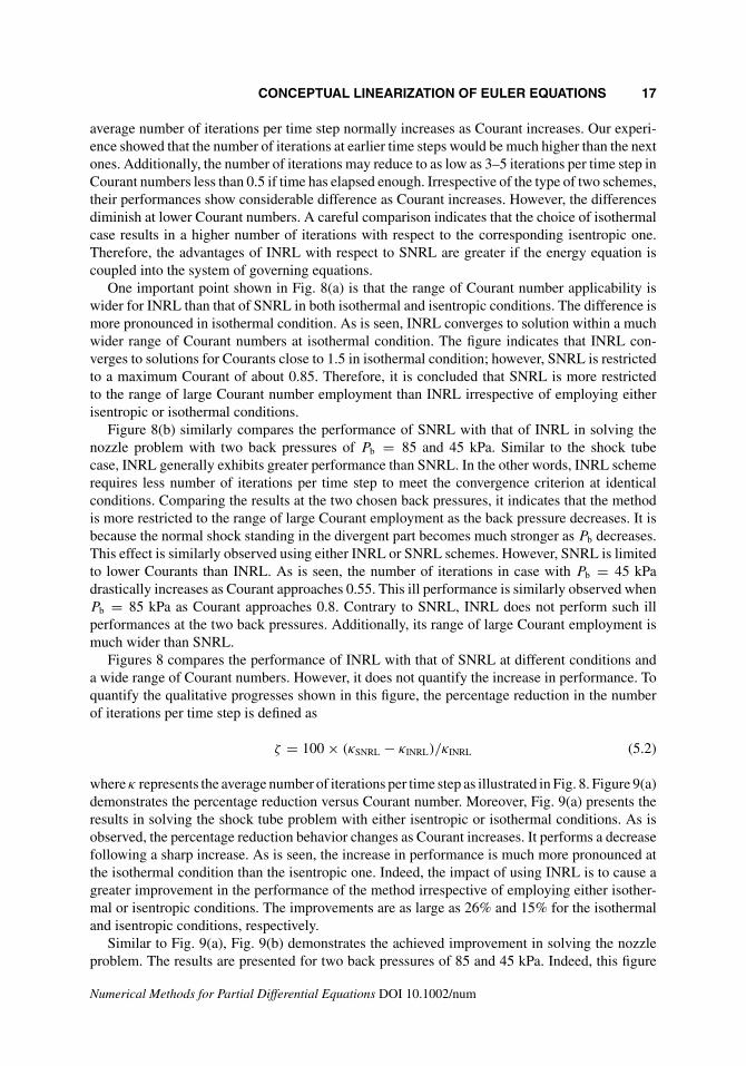
Figures 8 compares the performance of INRL with that of SNRL at different conditions anda wide range of Courant numbers. However, it does not quantify the increase in performance. Toquantify the qualitative progresses shown in this figure, the percentage reduction in the numberof iterations per time step is defined as
ζ = 100 × (κSNRL − κINRL)/κINRL (5.2)
where κ represents the average number of iterations per time step as illustrated in Fig. 8. Figure 9(a)demonstrates the percentage reduction versus Courant number. Moreover, Fig. 9(a) presents theresults in solving the shock tube problem with either isentropic or isothermal conditions. As isobserved, the percentage reduction behavior changes as Courant increases. It performs a decreasefollowing a sharp increase. As is seen, the increase in performance is much more pronounced atthe isothermal condition than the isentropic one. Indeed, the impact of using INRL is to cause agreater improvement in the performance of the method irrespective of employing either isother-mal or isentropic conditions. The improvements are as large as 26% and 15% for the isothermaland isentropic conditions, respectively.
Similar to Fig. 9(a), Fig. 9(b) demonstrates the achieved improvement in solving the nozzleproblem. The results are presented for two back pressures of 85 and 45 kPa. Indeed, this figure
Numerical Methods for Partial Differential Equations DOI 10.1002/num
18 DARBANDI, ROOHI, AND MOKARIZADEH
FIG. 9. The percentage reduction in the number of iterations versus Courant number. (a) The shock tubeproblem. (b) The nozzle problem.
quantifies the improvement illustrated in Fig. 8(b). As is observed, the improvement is excel-lent at both back pressures. Figure shows that INRL performs considerably better than SNRL intreating the steady compressible flow problem with shock, where a strong discontinuity stands inthe domain. The figure also indicates that the performance will be boosted up drastically if thenormal shock standing in the divergent part becomes stronger. In another words, the improvementin performance of INRL is considerable at lower back pressures. The improvement is dramatic asCourant approaches the limiting Courants. The improvements become as large as 42% and 80%for the cases with the weak and strong normal shocks, respectively.
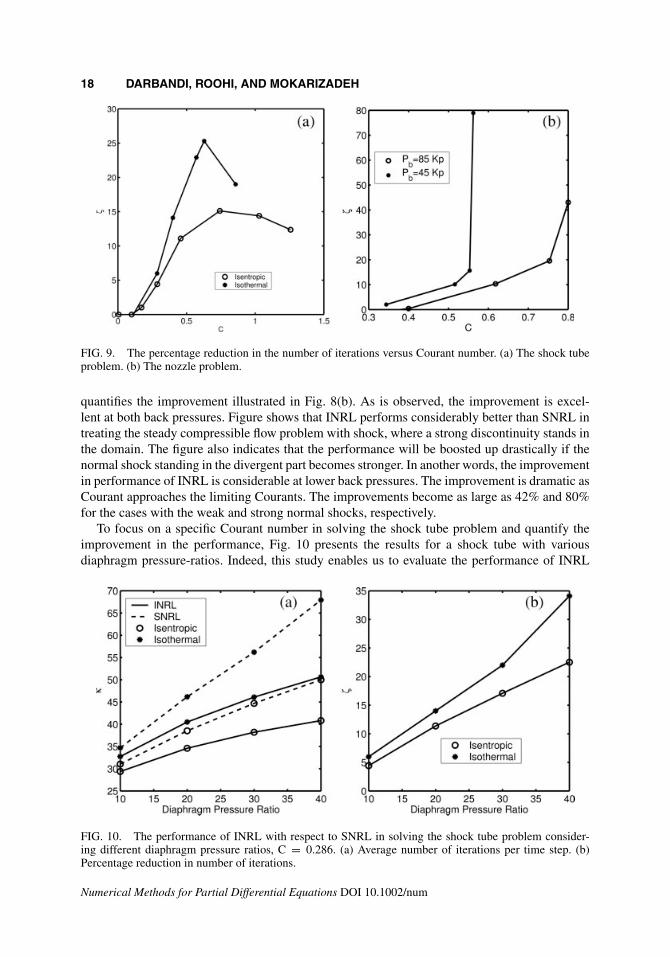
To focus on a specific Courant number in solving the shock tube problem and quantify theimprovement in the performance, Fig. 10 presents the results for a shock tube with variousdiaphragm pressure-ratios. Indeed, this study enables us to evaluate the performance of INRL
FIG. 10. The performance of INRL with respect to SNRL in solving the shock tube problem consider-ing different diaphragm pressure ratios, C = 0.286. (a) Average number of iterations per time step. (b)Percentage reduction in number of iterations.
Numerical Methods for Partial Differential Equations DOI 10.1002/num
CONCEPTUAL LINEARIZATION OF EULER EQUATIONS 19
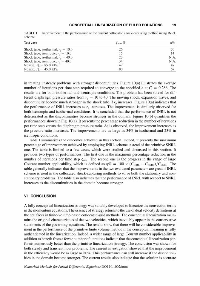
TABLE I. Improvement in the performance of the current collocated shock-capturing method using INRLscheme.
Test case ζmax% η%
Shock tube, isothermal, rp = 10.0 26 70Shock tube, isentropic, rp = 10.0 15 14Shock tube, isothermal, rp = 40.0 23 N.A.Shock tube, isentropic, rp = 40.0 34 N.A.Nozzle, Pb = 85.0 KPa 42 47Nozzle, Pb = 45.0 KPa 80 67
in treating unsteady problems with stronger discontinuities. Figure 10(a) illustrates the averagenumber of iterations per time step required to converge to the specified ε at C = 0.286. Theresults are for both isothermal and isentropic conditions. The problem has been solved for dif-ferent diaphragm pressure ratios from rp = 10 to 40. The moving shock, expansion waves, anddiscontinuity become much stronger in the shock tube if rp increases. Figure 10(a) indicates thatthe performance of INRL increases as rp increases. The improvement is similarly observed forboth isentropic and isothermal conditions. It is concluded that the performance of INRL is notdeteriorated as the discontinuities become stronger in the domain. Figure 10(b) quantifies theperformances shown in Fig. 10(a). It presents the percentage reduction in the number of iterationsper time step versus the diaphragm pressure ratio. As is observed, the improvement increases asthe pressure-ratio increases. The improvements are as large as 34% in isothermal and 23% inisentropic conditions.
Table I summarizes the outcomes achieved in this section. Indeed, it presents the maximumpercentage of improvement achieved by employing INRL scheme instead of the primitive SNRLone. The table is limited to a few cases, which were studied and discussed in this section. Itprovides two types of performances. The first one is the maximum percentage reduction in thenumber of iterations per time step ζmax. The second one is the progress in the range of largeCourant number applicability, which is defined as η% = 100 × (CINRL − CSNRL)/CSNRL. Thetable generally indicates that the improvements in the two evaluated parameters are great if INRLscheme is used in the collocated shock-capturing methods to solve both the stationary and non-stationary problems. The table also indicates that the performance of INRL with respect to SNRLincreases as the discontinuities in the domain become stronger.
VI. CONCLUSION
A fully conceptual linearization strategy was suitably developed to linearize the convection termsin the momentum equations. The essence of strategy returns to the use of dual velocity definitions atthe cell faces in finite-volume-based collocated-grid methods. The conceptual linearization main-tains the original characteristics of the two velocities, which inevitably appear in the conservativestatements of the governing equations. The results show that there will be considerable improve-ment in the performance of the primitive finite volume method if the conceptual meaning is fullyauthenticated in the linearization. Indeed, a wider range of large Courant number applicability inaddition to benefit from a fewer number of iterations indicate that the conceptual linearization per-forms numerously better than the primitive linearization strategy. The conclusion was shown forboth steady and transient flow problems. The current investigation showed that the improvementin the efficiency would be as large as 80%. This performance can still increase if the discontinu-ities in the domain become stronger. The current results also indicate that the solution is accurate
Numerical Methods for Partial Differential Equations DOI 10.1002/num
20 DARBANDI, ROOHI, AND MOKARIZADEH
enough in the regions with smooth to moderate variations and it is non-oscillatory in the regionswith discontinuities. This outcome is achieved without utilizing any types of numerical stabiliz-ers such as explicit artificial viscosity, explicit damping functions, and limiters. The conceptuallinearization does not deteriorate the accuracy at all. The advantages of the current linearizationstrategy can be equally reachable in the other finite-volume pressure-based collocated methods.
References
1. S. K. Godunov, A difference scheme for numerical computation of discontinuous solutions of fluiddynamics, Mat Sb 47 (1959), 271–306.
2. P. L. Roe, Approximate Riemann solvers, parameter vectors, and difference schemes, J Comput Phys43 (1981), 357–372.
3. A. Harten, P. D. Lax, and B. Van Leer, On upstream differencing and Godunov-type schemes forhyperbolic conservation laws, SIAM Rev 25 (1983), 35–61.
4. A. C. Berkenbosch, E. F. Kaasschieter, and J. H. M. Thije Boonkkamp, Finite-difference methodsfor one-dimensional hyperbolic conservation laws, Numer Methods Partial Differential Equations 10(1994), 225–269.
5. E. F. Toro, Riemann solvers and numerical methods for fluid dynamics, 2nd ed., Springer, Berlin, 1999.
6. V. Guinot, High resolution Godunov-type schemes with small stencils, Int J Numer Meth Fluids 44(2004), 1045–1162.
7. D. Choi and C. L. Merkle, Application of time-iterative schemes to incompressible flow, AIAA J 23(1985), 1518–1524.
8. R. Klein, Semi-implicit extension of a Godunov-type scheme based on low Mach number asymptoticsI: One-dimensional flow, J Comput Phys (1995), 213–237.
9. R. Codina, M. Vazquez, and O. C. Zienkiewicz, A general algorithm for compressible and incompressibleflows. III. The semi-implicit form, Int J Numer Methods Fluids 27 (1998), 13–32.
10. K. C. Karki and S. V. Patankar, Pressure based calculation procedure for viscous flows at all speeds inarbitrary configurations, AIAA J 27 (1989), 1167–1173.
11. F. S. Lien, A pressure-based unstructured grid method for all-speed flows, Int J Numer Methods Fluids33 (2000), 355–374.
12. M. Darbandi and S. F. Hosseinizadeh, General pressure-correction strategy to include density variationin incompressible algorithms, J Thermophysics Heat Transfer 17 (2003), 372–380.
13. D. R. van der Heul, C. Vuik, and P. Wesseling, A conservative pressure-correction method for flow atall speeds, Comput Fluids 32 (2003), 1113–1132.
14. S. F. Hosseinizadeh and M. Darbandi, A quasi-one-dimensional pressure-based solution for subsonicEuler flow regime, Far East J Appl Math 21 (2005), 157–171.
15. C. C. Rossow, A blended pressure/density based method for the computation of incompressible andcompressible flows, J Comput Phys 185 (2003), 375–398.
16. S. V. Patankar and D. B. Spalding, A calculation procedure for heat, mass, and momentum transfer inthree-dimensional parabolic flows, Int J Heat Mass Transfer 15 (1972), 1787–1806.
17. H. K. Versteeg and W. Malalasekera, An introduction to computational fluid dynamics; the finite volumemethod, Longman Scientific and Technical, Harlow, Essex, UK, 1995.
18. S. Thangam and D. D. Knight, A computational scheme in generalized coordinates for viscousincompressible flows, Computers Fluids 18 (1990), 317–327.
19. H. Bijl and P. Wesseling, A unified method for computing compressible and incompressible flows inboundary-fitted coordinates, J Comput Phys 141 (1998), 153–173.
Numerical Methods for Partial Differential Equations DOI 10.1002/num
CONCEPTUAL LINEARIZATION OF EULER EQUATIONS 21
20. M. Zijlema, A. Segal, and P. Wesseling, Invariant discretization of k − ε model in general co-ordinatefor prediction of turbulent flow in complicated geometries, Comput Fluids 24 (1995), 209–225.
21. M. Darbandi and M. Zakyani, Solving turbulent flow in curvilinear coordinate system using covariantvelocity calculation procedure, G. R. Liu, V. B. C. Tan, and X. Han, editors, Computational Methods,Springer, The Netherlands, 2006, pp. 161–175.
22. S. Faure, Stability of a colocated finite volume scheme for the Navier–Stokes equations, Numer MethodsPartial Differential Equations 21 (2004), 242–271.
23. C. M. Rhie and W. L. Chow, Numerical study of the turbulent flow past an airfoil with trailing edgeseparation, AIAA J 21 (1983), 1525–1532.
24. T. F. Miller and F. W. Schmidt, Use of a pressure-weighted interpolation method for the solution of theincompressible Navier–Stokes equations on a nonstaggered grid system, Numerical Heat Transfer 14(1988), 213–233.
25. H. Askoy and C. J. Chen, Numerical solution of Navier–Stokes equations with nonstaggered grids usingfinite analytic method, Numerical Heat Transfer B 21 (1992), 287–306.
26. M. M. Rahman, A. Miettinen, and T. Siikonen, Modified SIMPLE formulation on a collocated grid withan assessment of the simplified QUICK scheme, Numerical Heat Transfer B 30 (1996), 291–314.
27. A. W. Date, Complete pressure correction algorithm for solution of incompressible Navier–Stokesequations on a nonstaggered grid, Numerical Heat Transfer B 29 (1996), 441–458.
28. M. Darbandi and G. E. Schneider, Analogy-based method for solving compressible and incompressibleflows, J of Thermophysics and heat Transfer 12 (1998), 239–247.
29. M. Darbandi and S. F. Hosseinizadeh, A two-step modification toward implementing compressiblesource terms in low compressible flows, J Aerospace Science Technology 2 (2005), 37–44.
30. H. Paillère, P. Le Quèrè, C. Weisman, J. Vierendeels, E. Dick, M. Braack, F. Dabbene, A. Beccantini,E. Studer, T. Kloczko, C. Corre, V. Heuveline, M. Darbandi, and S. F. Hosseinizadeh, Modelling of nat-ural convection flows with large temperature differences: A benchmark problem for low mach numbersolvers, Part 2: ESAIM: Mathematical Modelling and Numerical Analysis 39 (2005), 617–621.
31. M. Darbandi and S. F. Hosseinizadeh, Numerical simulation of thermobuoyant flow with largetemperature variation, J Thermophys Heat Transfer 20 (2006), 285–296.
32. J. P. Van Doormal, G. D. Raithby, and B. H. McDonald, The segregated approach to predicting viscouscompressible fluid flows, J Turbomachinery 109 (1987), 268–277.
33. J. C. Tannehill, R. S. Pletcher, and D. A. Anderson, Computational fluid mechanics and heat transfer,Taylor and Francis, Washington, 1997.
34. R. I. Issa, Solution of the implicitly discretized fluid flow equations by operator-splitting, J ComputPhys 62 (1986), 40–65.
35. R. I. Issa and M. H. Javareshkian, Pressure-based compressible calculation method utilizing totalvariation diminishing schemes, AIAA J 36 (1998), 1652–1657.
36. N. W. Bressloff, A parallel pressure implicit splitting of operators algorithm applied to flows at allspeeds, Int J Numer Methods Fluids 36 (2001), 497–617.
37. M. Darbandi and G. E. Schneider, Momentum variable procedure for solving compressible andincompressible flows, AIAA J 35 (1997), 1801–1805.
38. M. Darbandi and G. E. Schneider, Comparison of pressure-based velocity and momentum proceduresfor shock tube problem, Numerical Heat Transfer B 33 (1998), 287–300.
39. M. Darbandi and G. E. Schneider, Performance of an analogy-based all-speed procedure without anyexplicit damping, Comput Mech 26 (2000), 459–469.
40. S. F. Wornom and M. M. Hafez, Implicit conservative schemes for the Euler equations, AIAA J 24(1986), 215–223.
Numerical Methods for Partial Differential Equations DOI 10.1002/num
22 DARBANDI, ROOHI, AND MOKARIZADEH
41. D. A. Venditti and D. L. Darmofal, Adjoint error estimation and grid adaption for functional outputs:application to quasi-one-dimensional flow, J Comput Phys 164 (2000), 204–227.
42. C. C. Rossow, Extension of a compressible code toward the incompressible limit, AIAA J 41 (2003),2379–2386.
43. J. Y. Yang, F. S. Lien, and C. A. Hsu, Non-oscillatory shock capturing finite element methods for theone-dimensional compressible Euler equations, Int J Numer Methods Fluids 11 (1990), 405–426.
44. M. Darbandi and S. M. Bostandoost, A new formulation toward unifying the velocity role in collocatedvariable arrangement, Numerical Heat Transfer B 47 (2005), 361–382.
45. M. Darbandi and V. Mokarizadeh, A modified pressure-based algorithm to solve the flow fields withshock and expansion waves, Numerical Heat Transfer B 46 (2004), 497–504.
46. C. Prakash and S. V. Patankar, A control volume-based finite-element method for solving the Navier–Stokes equations, using equal-order velocity-pressure interpolation, Numerical Heat Transfer 8 (1985),259–280.
47. G. E. Schneider and M. J. Raw, Control volume finite element method for heat transfer and fluid flowusing co-located variables - 1.Computational procedure, Numerical Heat Transfer 11 (1987), 363–390.
48. M. Sun and K. Takayama, An artificially upstream flux vector splitting scheme for the Euler equations,J Comput Phys 189 (2003), 305–329.
49. V. A. Titarev and E. F. Toro, WENO schemes based on upwind and centered TVD fluxes, Comput Fluids34 (2005), 705–720.
Numerical Methods for Partial Differential Equations DOI 10.1002/num