Concepts Review - McGraw Hill Educationhighered.mheducation.com/sites/dl/free/0077454898/838388/EOL_Excel... · Exit Protected View if necessary. e ... Tab to move from one entry

EX-397LESSON 9 Using What-If Analysis ToolsUN

IT 3 LESSON

9True/False QuestionsEach of the following statements is either true or false. Indicate your choice by circling T or F.

1. Color scales are best described as what-if analysis.

2. A scenario summary report is created on its own sheet.

3. Goal Seek uses parameters to set restrictions on each cell.

4. A trendline highlights the most common data points in a series.

5. You can use named ranges or cell addresses to build a scenario.

6. The purpose of what-if analysis is to use an IF statement in more than one formula.

7. The Research tool can include an encyclopedia, a thesaurus, and translation dictionaries.

8. In Solver, you can have more than one adjustable cell.

Short Answer QuestionsWrite the correct answer in the space provided.

1. What Solver term describes a limitation or restriction on a cell?

2. What does the Thesaurus component of the Research tool do?

3. How would you create the following label: José?

4. Name two document properties that you can set and edit.

5. What are the three types of data visualizations that are part of conditional formatting options?

6. In a scenario summary report, what do the expand and collapse buttons do?

Concepts Review

T F

T F

T F

T F

T F

T F

T F

T F

ste31214_ch09_EX366-EX409.indd Page EX-397 20/04/10 9:36 PM user-f467ste31214_ch09_EX366-EX409.indd Page EX-397 20/04/10 9:36 PM user-f467 /Volumes/203/MHRL033/ros69760_disk1of1/0070969760/ros69760_pagefiles/Volumes/203/MHRL033/ros69760_disk1of1/0070969760/ros69760_pagefile

UNIT 3 Presenting and Analyzing Worksheet DataEX-398

7. What term might be described as what-if analysis in reverse?

8. What is a trendline?

Critical ThinkingAnswer these questions on a separate page. There are no right or wrong answers. Support your answers with examples from your own experience, if possible.

1. What types of problems might arise for a company from using the Research tools in a workbook?

2. Think of what-if analysis problems that you face as an employee or a student. How could you use the tools covered in this lesson, such as trendlines, Goal Seek, and Solver?

UNIT

3

LESS

ON 9

Exercise 9-24Monitor workbook security. Create scenarios. Set conditional formatting. Manage scenarios.

AllAround Vision Care sells a specialty eyeglass frame made from environmentally friendly materials. From each sale, a contribution of $3 is made to Better Planet, an ecological nonprofit organization. In the worksheet, you need to calculate the contribution amounts for the fourth quarter. From the projected data, you will create scenarios with a related summary report. The workbook does have a macro and has been marked as final.

1. Monitor workbook security by following these steps:

a. Click the File command tab and choose Options.

b. Click Trust Center. Click Trust Center Settings. Click Macro Settings.

c. Click to select Disable all macros with notification if it is not selected. Click OK to close the Trust Center. Click OK again.

d. Open Excel_SR9-24, a macro-enabled workbook. Exit Protected View if necessary.

e. In the Security Warning bar, click Enable this content.

f. Click Edit Anyway to turn off this property.

g. Click the View command tab. Click the Macros button . Choose CompanyName and click Run. Make the label bold.

h. Press F12 and name the workbook [your initials]9-24.

Skills Review


EX-399LESSON 9 Using What-If Analysis Tools

i. Click the Save as type arrow and choose Excel Workbook.

j. Click Save. Click Yes.

2. Create scenarios by following these steps:

a. Select cells B3:E4. Click the Formulas command tab. Click the Create from Selection button . Use the top row for range names. Click OK.

b. Name cell B5 as OctDollars. Name cell C5 as NovDollars and cell D5 as DecDollars. Name cell E5 as TotalDollars.

c. Click the Name Manager button and choose New. Key Contribution as the name. In the Refers to box, key =3 to create a constant. Close the dialog box.

d. Click cell B6 and key =. Click cell B4 and key *cont. Press Tab and then press Enter . Copy this formula to cell E6. All the formulas use the named range Oct.

e. Click cell B6 and key =b4*cont. Press Tab and then press Enter . Copy this formula to cell E6. Cell references are relative.

f. Format the results as accounting.

g. Select cells B4:D4. Click the Data command tab. Click the What-If Analysis button . Choose Scenario Manager. Click Add.

h. In the Scenario name box, key Modest Sales. Press Tab .

i. In the Changing cells box, note that the selected cells are listed. Press Tab .

j. In the Comment box, key Assumes modest sales. Click OK.

k. Do not change any values. Click OK.

l. Click Add. Key Best Sales as the name. Press Tab . Keep the same Changing cells box.

m. Press Tab . For the Comment, key Assumes high sales. Click OK.

n. Key the following values for each of the changing cells:

Oct 180 Nov 200 Dec 190

o. Click OK. Click Add.

p. Add a scenario named Worst Sales with the Comment Assumes low sales. and the values shown here.

Oct 90 Nov 100 Dec 95

q. Click OK. Click Close.

UNIT 3

LESSON 9

NOTE

This worksheet includes a named constant for the price.

NOTE

Range names are absolute references in a formula.

TIP

While the default comment is selected, key the new one to replace it.

REVIEW

Press Tab to move from one entry box to the next in the Scenario Values

dialog box.



3. Set conditional formatting by following these steps:

a. Select cells B4:D4 and click the Home command tab.

b. Click the Conditional Formatting button and choose Color Scales.

c. Choose the two-color scale Green-Yellow.

d. Select cells B5:D5 and click the Conditional Formatting button . Choose Highlight Cells Rules and More Rules.

e. Choose Cell Value.

f. Choose greater than or equal to.

g. Click in the rightmost text box and key 12000.

h. Click Format. On the Font tab, choose Bold Italic. For Color choose Green from the Standard Colors.

i. Close the dialog boxes.

4. Manage scenarios by following these steps:

a. Click the Data command tab. Click the What-If Analysis button .

b. Choose Scenario Manager.

c. Choose Worst Sales in the list and click Edit.

d. Change the value for October to 75. Click Show.

e. In the Scenario Manager dialog box, click Summary. Choose Scenario summary.

f. In the Result cells box, select the range B5:E5. Click OK.

5. Select cells B7:D7 on the 4thQtr worksheet. Click the Home command tab and click the arrow with the Merge and Center button . Choose the option to merge the cells. Wrap the text and set it for middle and center alignment. Adjust the row height as needed. Center the page horizontally.

6. Prepare and submit your work.

Exercise 9-25Set conditional formatting. Manage scenarios. Forecast with a trendline.

Gas-permeable contact lenses have been sold for many years by eye professionals, and AllAround Vision Care keeps sales data. The workbook includes scenarios, but some of the data have been adjusted, and you need to make those edits. Instead of a color scale, you have decided to use icon sets for your conditional formatting. In a related chart, the company would like to project 6 months’ sales for the higher than expected sales scenario.

1. Open Excel_SR9-25 and remove the Marked as Final property. Save the workbook as [your initials]9-25.

2. Set conditional formatting by following these steps:

a. Select cells B4:D4 and click the Home command tab.

b. Click the Conditional Formatting button and choose Icon Sets.

c. Choose 3 Arrows (Colored).

UNIT

3

LESS

ON 9




a. Click the Data command tab.

b. Click the What-If Analysis button . Choose Scenario Manager.

c. Edit the High Sales scenario to show these changing cells:

Oct 75Nov 85Dec 95

d. Show the High Sales scenario.

e. From the Scenario Manager dialog box, create a Scenario summary report using cells B5:E5 as the Result cells.

f. Expand row 3 to display the scenario comments.

4. Select cells B3:D4 on the 4thQtr sheet and create a column chart sheet. Add a chart title above the chart that displays Projected Sales of Gas Permeable Lenses. Choose chart Style 27.

5. Forecast with a trendline by following these steps:

a. Click the Chart Tools Layout tab.

b. Click the Trendline button . Choose More Trendline Options.

c. Choose Logarithmic in the Trend/Regression Type group.

d. In the Trendline Name group, choose Custom. Key Next 6 Months in the Custom box.

e. In the Forecast Forward box, key 6.

f. Click Line Style.

g. Use a 3-point width. Choose Long Dash for the Type. For the End type in the Arrow settings group, choose Open Arrow. Click Close.

h. On the Chart Tools Design tab, click the Select Data button . Name the first series as Pairs Sold.


Exercise 9-26Use Goal Seek. Use Solver. Manage scenarios.

In this workbook, your first task is to use Goal Seek with two financial functions already calculated by the human resources personnel. One formula determines a monthly car payment for a loan, and you would like to know how much can be borrowed if you can afford a $350 monthly payment. This same worksheet has another formula that calculates how much money you’ll have in an account if you save a particular amount each month. On another worksheet, AllAround Vision Care has tallied the number of gallons of water saved by the new faucets and drinking fountains. You’ve been asked to use Solver to calculate how the company could increase its savings to a specified dollar amount.

UNIT 3

LESSON 9

NOTE

A logarithmic line is a curved line and is suited to values that increase or decrease

quickly and then level out.

ste31214_ch09_EX366-EX409.indd Page EX-401 5/15/10 1:06 PM user-f468ste31214_ch09_EX366-EX409.indd Page EX-401 5/15/10 1:06 PM user-f468 /Users/user-f468/Desktop/Nalini 13.4/Davis/ch07/Users/user-f468/Desktop/Nalini 13.4/Davis/ch07


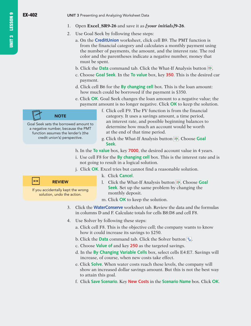
1. Open Excel_SR9-26 and save it as [your initials]9-26.

2. Use Goal Seek by following these steps:

a. On the CreditUnion worksheet, click cell B9. The PMT function is from the financial category and calculates a monthly payment using the number of payments, the amount, and the interest rate. The red color and the parentheses indicate a negative number, money that must be spent.

b. Click the Data command tab. Click the What-If Analysis button .

c. Choose Goal Seek. In the To value box, key 350. This is the desired car payment.

d. Click cell B6 for the By changing cell box. This is the loan amount: how much could be borrowed if the payment is $350.

e. Click OK. Goal Seek changes the loan amount to a negative value; the payment amount is no longer negative. Click OK to keep the solution.

f. Click cell F9. The FV function is from the financial category. It uses a savings amount, a time period, an interest rate, and possible beginning balances to determine how much an account would be worth at the end of that time period.

g. Click the What-If Analysis button . Choose Goal Seek.

h. In the To value box, key 7000, the desired account value in 4 years.

i. Use cell F8 for the By changing cell box. This is the interest rate and is not going to result in a logical solution.

j. Click OK. Excel tries but cannot find a reasonable solution.

k. Click Cancel.

l. Click the What-If Analysis button . Choose Goal Seek. Set up the same problem by changing the monthly deposit.

m. Click OK to keep the solution.

3. Click the WaterConserve worksheet tab. Review the data and the formulas in columns D and F. Calculate totals for cells B8:D8 and cell F8.

4. Use Solver by following these steps:

a. Click cell F8. This is the objective cell; the company wants to know how it could increase its savings to $250.

b. Click the Data command tab. Click the Solver button .

c. Choose Value of and key 250 as the targeted savings.

d. In the By Changing Variable Cells box, select cells E4:E7. Savings will increase, of course, when new costs take effect.

e. Click Solve. When water costs reach these levels, the company will show an increased dollar savings amount. But this is not the best way to attain this goal.

f. Click Save Scenario. Key New Costs in the Scenario Name box. Click OK.

UNIT

3

LESS

ON 9

NOTE

Goal Seek sets the borrowed amount to a negative number, because the PMT

function assumes the lender’s (the credit union’s) perspective.

REVIEW

If you accidentally kept the wrong solution, undo the action.



g. Choose Restore Original Values. Click OK.

h. Click the Solver button . The objective cell and the value setting are the same.

i. In the By Changing Variable Cells box, select cells C4:C7. Some adjustments can be made to the equipment to increase the number of gallons saved per hour.

j. Click Add in the Subject to the Constraints group.

k. In the Cell Reference box, click cell C4. Click the arrow for the middle (operator) box and choose <=. In the Constraint box, key 6. The equipment is limited in how it can be adjusted.

l. Click Add. In the Cell Reference box, select cell C5. Choose <= as the operator. In the Constraint box, key 10. Click Add.

m. In the Cell Reference box, select cell C6. Choose <= as the operator and set 7.5 as the Constraint. Click OK.

n. Click Solve.

o. Click Save Scenario. Key Increased per Hour and click OK.

p. Choose Restore Original Values. Click OK.


a. Click the Data command tab.

b. Click the What-If Analysis button . Choose Scenario Manager.

c. Create a Scenario summary report using cell F8 as the Result cells setting.

6. Click the File command tab. Choose Protect Workbook and then Mark as Final. Click OK in both message boxes. Close Backstage view.


Exercise 9-27Monitor workbook security. Use the Research tool. Work with the Info pane.

As preparation for increased sales from Latin America and Mexico, AllAround Vision Care wants to promote several eyeglass frames on its Web site using Spanish names. You are to use the Translation tool to find substitute Spanish names.

1. Open Excel_SR9-27 and remove the Marked as Final property. Save the workbook as [your initials]9-27.

2. Use the Research tool by following these steps:

a. Click cell A5. Click the Review command tab. Click the Translate button .

b. Click the Expand icon for Translation in the Research task pane.

c. In the To box, choose Spanish (International Sort). Click the Expand icon for Bilingual dictionary if the list is not expanded.

d. Click cell B5 and key Luna Azul.

UNIT 3

LESSON 9

TIP

Key spaces between words in scenario names so that the summary report

includes spaces in the names.

NOTE

Solver can often find more than one solution to a problem; each time you run it, you may see slightly different results.



e. Click cell A6. Click the Translate button . The translation for “cat” is “gato.”

f. In the Search For box, delete Cat leaving Eyes. Click the Start Searching button .

g. Click cell B6 and key Ojos de Gato.

h. Click cell A7. Click the Translate button .

i. Review the results. In cell B7 key Luz del D. Do not complete the entry.

j. In Edit mode for cell B7, click the Insert command tab. In the Symbols group, click the Symbol button .

k. Set the Font to Calibri and the Subset to Basic Latin.

l. Find í, the accented lowercase “i.” This is an acute accent. Click the character and click Insert. Click Close.

m. Key a to complete the entry as “Luz del Día.”

n. Find Spanish words for the remaining two frame names.

o. Insert a row at row 3. In cell A3 key Discovery en Espa. The next character is an accented lowercase n (ñ).

p. In Edit mode for cell A3, click the Insert tab. Click the Symbol button .

q. Set the Font to Calibri and the Subset to Basic Latin.

r. Find ñ, the accented lowercase “n.” This is a tilde accent. Click the character and click Insert. Click Close.

s. Complete the label in cell A3 to show “Discovery en Español.”

3. Work with the Info pane by following these steps:

a. Press Ctrl + Home . Click the File tab.

b. Click the arrow with Properties and choose Advanced Properties.

c. Click the Summary tab. In the Author box, key [your first and last name].

d. In the Title box, key Spanish Frame Names.

e. Key AllAround Vision Care as the company name.

f. Click to select Save Thumbnails for All Excel Documents.

g. Close the dialog box and then close Backstage view.


UNIT

3

LESS

ON 9

NOTE

Translation dictionaries assume that you understand the grammar of the

selected language.


EX-405LESSON 9 Using What-If Analysis ToolsUN

IT 3 LESSON

9

Lesson Applications

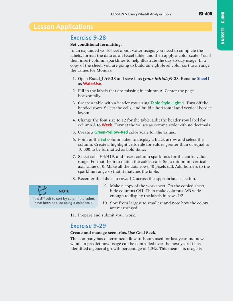
Exercise 9-28Set conditional formatting.

In an expanded worksheet about water usage, you need to complete the labels, format the data as an Excel table, and then apply a color scale. You’ll then insert column sparklines to help illustrate the day-to-day usage. In a copy of the sheet, you are going to build an eight-level color sort to arrange the values for Monday.

1. Open Excel_LA9-28 and save it as [your initials]9-28. Rename Sheet1 as WaterUse.

2. Fill in the labels that are missing in column A. Center the page horizontally.

3. Create a table with a header row using Table Style Light 1. Turn off the banded rows. Select the cells, and build a horizontal and vertical border layout.

4. Change the font size to 12 for the table. Edit the header row label for column A to Week. Format the values as comma style with no decimals.

5. Create a Green-Yellow-Red color scale for the values.

6. Point at the Sat column label to display a black arrow and select the column. Create a highlight cells rule for values greater than or equal to 10,000 to be formatted as bold italic.

7. Select cells H4:H19, and insert column sparklines for the entire value range. Format them to match the color scale. Set a minimum vertical axis value of 0. Make all the data rows 40 pixels tall. Add borders to the sparkline range so that it matches the table.

8. Recenter the labels in rows 1:2 across the appropriate selection.

9. Make a copy of the worksheet. On the copied sheet, hide columns C:H. Then make columns A:B wide enough to display the labels in rows 1:2.

10. Sort from largest to smallest and note how the colors are rearranged.


Exercise 9-29Create and manage scenarios. Use Goal Seek.

The company has determined kilowatt-hours used for last year and now wants to predict how usage can be controlled over the next year. It has identified a general growth percentage of 1.5%. This means its usage is

NOTE

It is difficult to sort by color if the colors have been applied using a color scale.

ste31214_ch09_EX366-EX409.indd Page EX-405 6/10/10 12:43 AM user-f468ste31214_ch09_EX366-EX409.indd Page EX-405 6/10/10 12:43 AM user-f468/Volumes/202/MH00543_r1/hin73516_disk1of1/0073373516/Access_Archive/hin73516_.../Volumes/202/MH00543_r1/hin73516_disk1of1/0073373516/Access_Archive/hin73516_

EX-406 UNIT 3 Presenting and Analyzing Worksheet Data

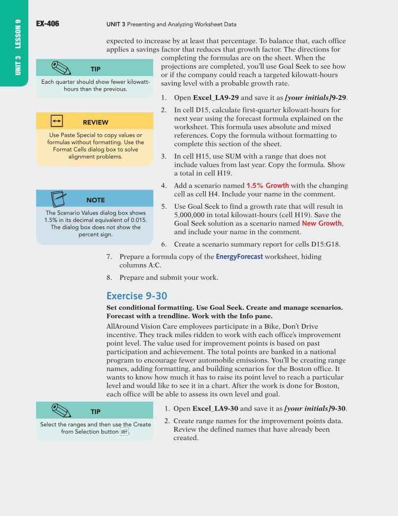
expected to increase by at least that percentage. To balance that, each office applies a savings factor that reduces that growth factor. The directions for

completing the formulas are on the sheet. When the projections are completed, you’ll use Goal Seek to see how or if the company could reach a targeted kilowatt-hours saving level with a probable growth rate.

1. Open Excel_LA9-29 and save it as [your initials]9-29.

2. In cell D15, calculate first-quarter kilowatt-hours for next year using the forecast formula explained on the worksheet. This formula uses absolute and mixed references. Copy the formula without formatting to complete this section of the sheet.

3. In cell H15, use SUM with a range that does not include values from last year. Copy the formula. Show a total in cell H19.

4. Add a scenario named 1.5% Growth with the changing cell as cell H4. Include your name in the comment.

5. Use Goal Seek to find a growth rate that will result in 5,000,000 in total kilowatt-hours (cell H19). Save the Goal Seek solution as a scenario named New Growth, and include your name in the comment.

6. Create a scenario summary report for cells D15:G18.

7. Prepare a formula copy of the EnergyForecast worksheet, hiding columns A:C.


Exercise 9-30Set conditional formatting. Use Goal Seek. Create and manage scenarios. Forecast with a trendline. Work with the Info pane.

AllAround Vision Care employees participate in a Bike, Don’t Drive incentive. They track miles ridden to work with each office’s improvement point level. The value used for improvement points is based on past participation and achievement. The total points are banked in a national program to encourage fewer automobile emissions. You’ll be creating range names, adding formatting, and building scenarios for the Boston office. It wants to know how much it has to raise its point level to reach a particular level and would like to see it in a chart. After the work is done for Boston, each office will be able to assess its own level and goal.


2. Create range names for the improvement points data. Review the defined names that have already been created.

UNIT

3

LESS

ON 9

TIP

Each quarter should show fewer kilowatt-hours than the previous.

TIP

Select the ranges and then use the Create from Selection button .

REVIEW

Use Paste Special to copy values or formulas without formatting. Use the

Format Cells dialog box to solve alignment problems.

NOTE

The Scenario Values dialog box shows 1.5% in its decimal equivalent of 0.015.

The dialog box does not show the percent sign.



3. From the Review command tab, run Spelling and make corrections as needed.

4. Create a highlight cells rule to show improvement points greater than 3,000 in bold green italic.

5. Create a scenario named Boston1 for cell D20.

6. Use Goal Seek to find an improvement point level for Boston that would result in 45,000 in total points (cell F17). This means that Boston is being asked to increase its points but the other cities are not. Save the Goal Seek solution as a scenario named Boston2.

7. Create a scenario summary report for cells B13:E13. In the report, edit the labels in column C to show the quarter names.

8. Show the Boston2 scenario, and create a line chart for cells B12:E13 on a separate sheet. Add a title and format the line chart. Add and format a trendline that projects points for four quarters.

9. Edit the document properties to show your name as the author and AllAround Vision Care as the company. Include a thumbnail.


Exercise 9-31 Challenge YourselfUse Solver. Create and manage scenarios. Work with the Info pane.

The Dallas office of AllAround Vision Care wants to optimize its advertising dollars. It will use Solver to determine the lowest media cost that will result in the most exposures (number of times an ad is heard or seen). The worksheet lists three media with estimated audience numbers and costs. You will complete the worksheet and formulas and use Solver to calculate the best combination of media.


2. Name cell F12 as TotalExposure. Name cells C10:E10 as TotalCost. Name cells C11:E11 as SampleRun. Finally, name cells C8:E8 as EstimatedRun.

3. In row 11, build a formula to calculate how many ads can be run based on the money allocated to the media.

4. In row 12, build a formula to determine the number of exposures if the sample number of ads is run at the indicated cost per ad.

5. In cell F10, build a formula that sums all amounts allocated. In cell F12, build a formula that sums total exposures.

UNIT 3

LESSON 9

NOTE

Although the amount of money to allocate is not yet determined, you can

use that cell in a formula.

REVIEW

Select the cell range and click the Name Box. Key the range name and press Enter . Press F3 to see a list of defined names in

the workbook.



6. Add a scenario named Original for the worksheet as it exists. Set the range named “TotalCost” for the changing cells.

7. Use Solver to find the minimum amount for cell F10 by changing the “TotalCost” range. The constraints are as follows:

C11 >= 8 D11 >= 10 E11 >= 5 TotalCost >= 0 TotalExposure >= 5000000

8. Save the Solver solution as a scenario named Scenario 1 and display it.

9. Create a scenario summary report with cell F10 as a result cell. In rows below the main report, key an explanation for each constraint used in the Solver problem.

10. Insert a new sheet and paste a list of range names. Supply labels and your own formatting. Name this sheet Documentation.

11. Edit document properties to show your name as the author and AllAround Vision Care as the company. Include a thumbnail.


UNIT

3

LESS

ON 9

On Your Own

In these exercises you work on your own, as you would in a real-life work environment. Use the skills you’ve learned to accomplish the task—and be creative.

Exercise 9-32In a new workbook, key labels, values, and formulas for a sports activity with which you are familiar. Use players or team names, scores, or other statistics that you know or can locate. Make your own format choices. Save your first set of scores or statistics as a scenario. Create best-case and worst-case scenarios for your players and teams. Create a scenario summary report. Save the workbook as [your initials]9-32. Prepare and submit your work.



Exercise 9-33Create a workbook that lists dates starting at today and continuing for 30 days from now in one column. In the second column, show the day of the week (Monday, Tuesday). In the third column, enter values to represent the number of phone calls, e-mails, or text messages that you received, either at home or the office. In the fourth column, enter values to represent the number of calls or messages that you sent. Apply a color scale. Then experiment using highlight cells rules that you create. Add labels and other formatting effects to prepare a professional worksheet. Save the workbook as [your initials]9-33. Prepare and submit your work.

Exercise 9-34In a new workbook, key the names and costs of five items or activities that you would like to buy or do (new TV, trip to Paris, donating to a charity, etc.). Sum the cost of purchasing or doing one of each item or activity. Use Solver to find three target totals that are lower than the actual total by changing the price or cost of one or more of the items. If Solver cannot find a solution or finds an unacceptable one, try adding constraints. Solve for reasonable amount, and save each possibility as a scenario. After you have completed your analysis, make a copy of the sheet and translate each item name into a language for which the dictionary is available on your computer. Save the workbook as [your initials]9-34. Prepare and submit your work.

UNIT 3

LESSON 9
