Concepts of DSP (Digital Signal Processing) and use of DTT

1

KAGRA Lecture 3 for students 16.08.2018

Concepts of DSP (Digital Signal Processing) and use of DTT (diaggui) for

TF measurements

Enzo TapiaLecture 3

2


What is Digital Signal Prossesing?

DSP is different from other areas of computer science because it uses signals. And we get these signals normally using a sensor that measures data from real world, like vibrations, images, sound, etc. An analog-to-digital converter is needed in the real world to take analog signals and convert them into 0's and 1's for a digital format.

DSP is the mathematics, algorithms and the techniques used to manipulate this signals.

While an analog system (filter as example) would use amplifiers, capacitors, inductors, or resistors, and be affordable and easy to assemble, it would be difficult to calibrate or modify the filter order. However, the same things can be done with a DSP system, which is easier to design and modify (Software-based).

3


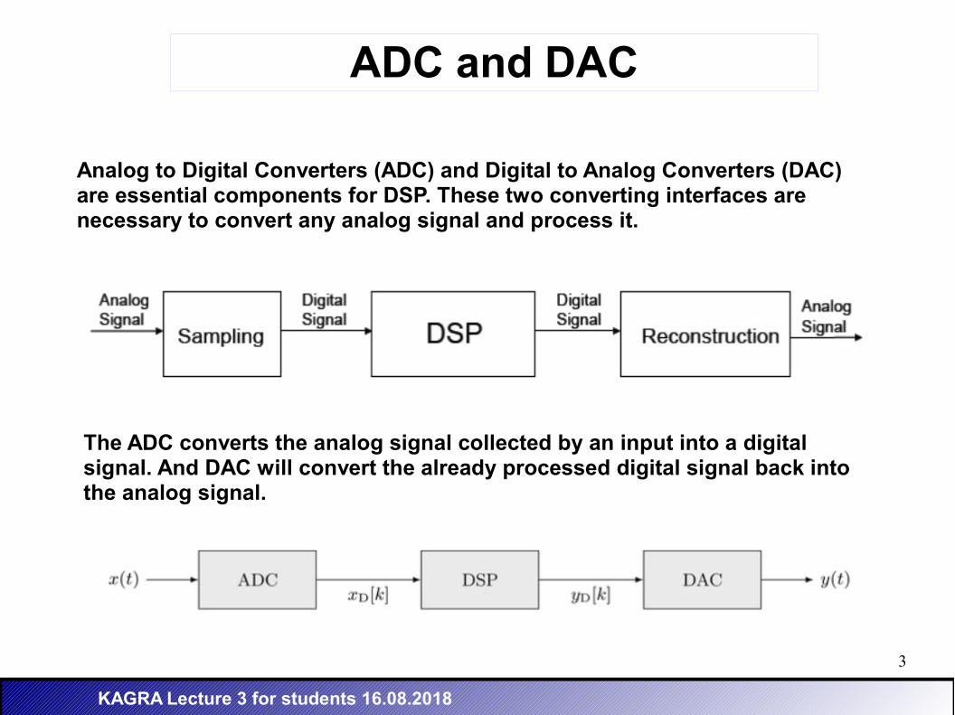
ADC and DAC

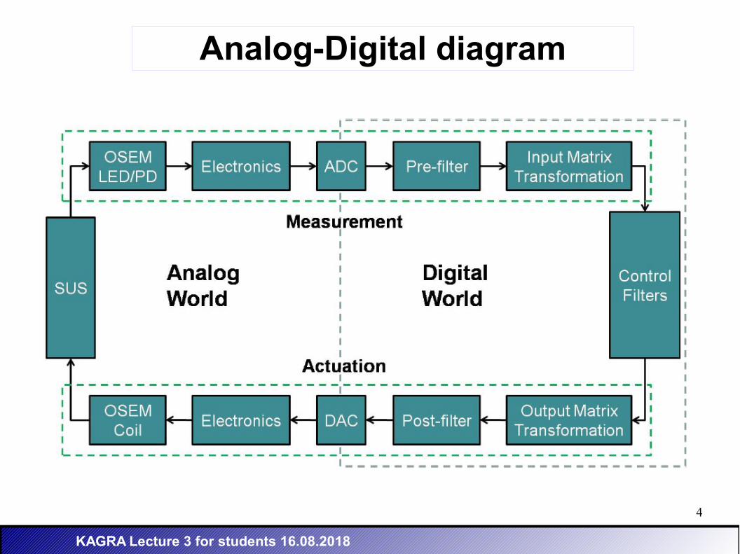
Analog to Digital Converters (ADC) and Digital to Analog Converters (DAC) are essential components for DSP. These two converting interfaces are necessary to convert any analog signal and process it.

The ADC converts the analog signal collected by an input into a digital signal. And DAC will convert the already processed digital signal back into the analog signal.

4


Analog-Digital diagram

5


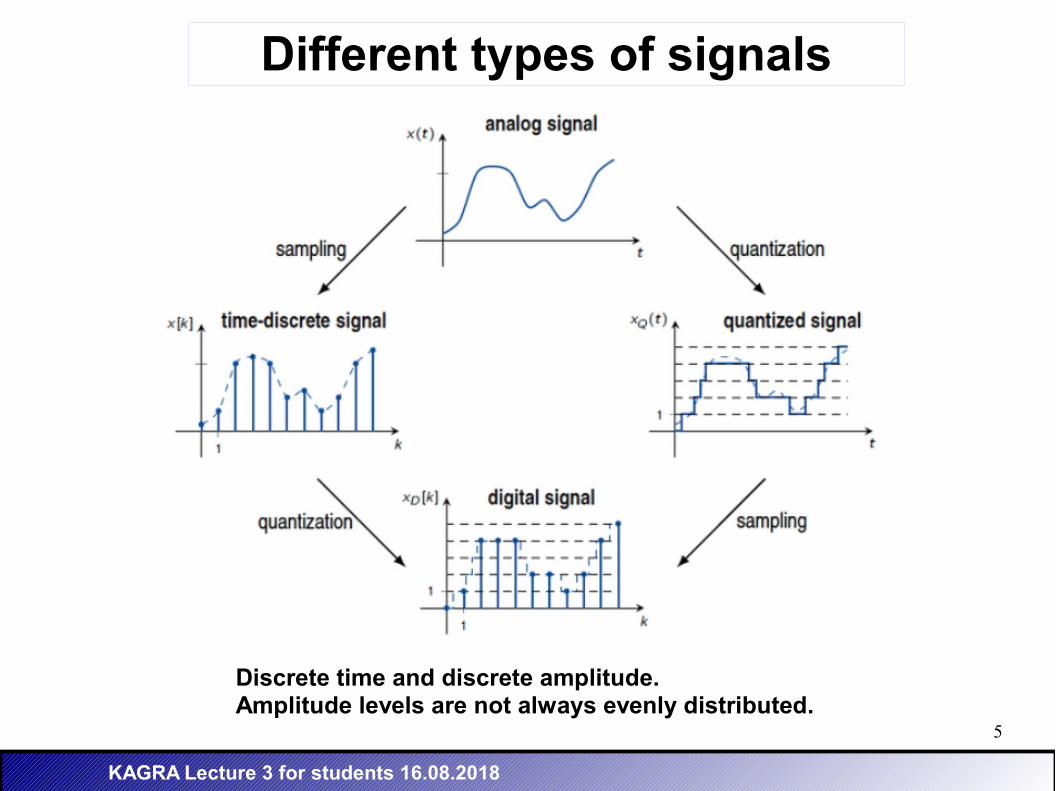
Different types of signals

Discrete time and discrete amplitude.Amplitude levels are not always evenly distributed.

6


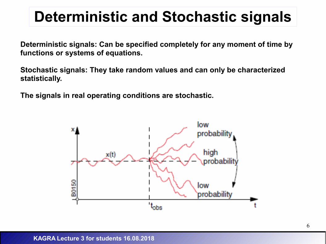
Deterministic and Stochastic signals

Deterministic signals: Can be specified completely for any moment of time by functions or systems of equations.

Stochastic signals: They take random values and can only be characterized statistically.

The signals in real operating conditions are stochastic.

7


Analysis in frequency domain 1

There are two ways to perform the analysis in frequency, one is through the FFT analyzer and another is through digital filtering. The principle of Fourier analysis is that every periodic function can be represented by a series of sines and cosines.

To obtain the vibration amplitudes of each frequency it is necessary perform a frequency analysis. For this purpose a filter is used that only allows pass those parts of the vibration that are contained in a narrow range of frequencies. The bandwidth of the filter used moves continuously throughout of the entire frequency range of interest to obtain the separate vibration levels for each frequency band.

8



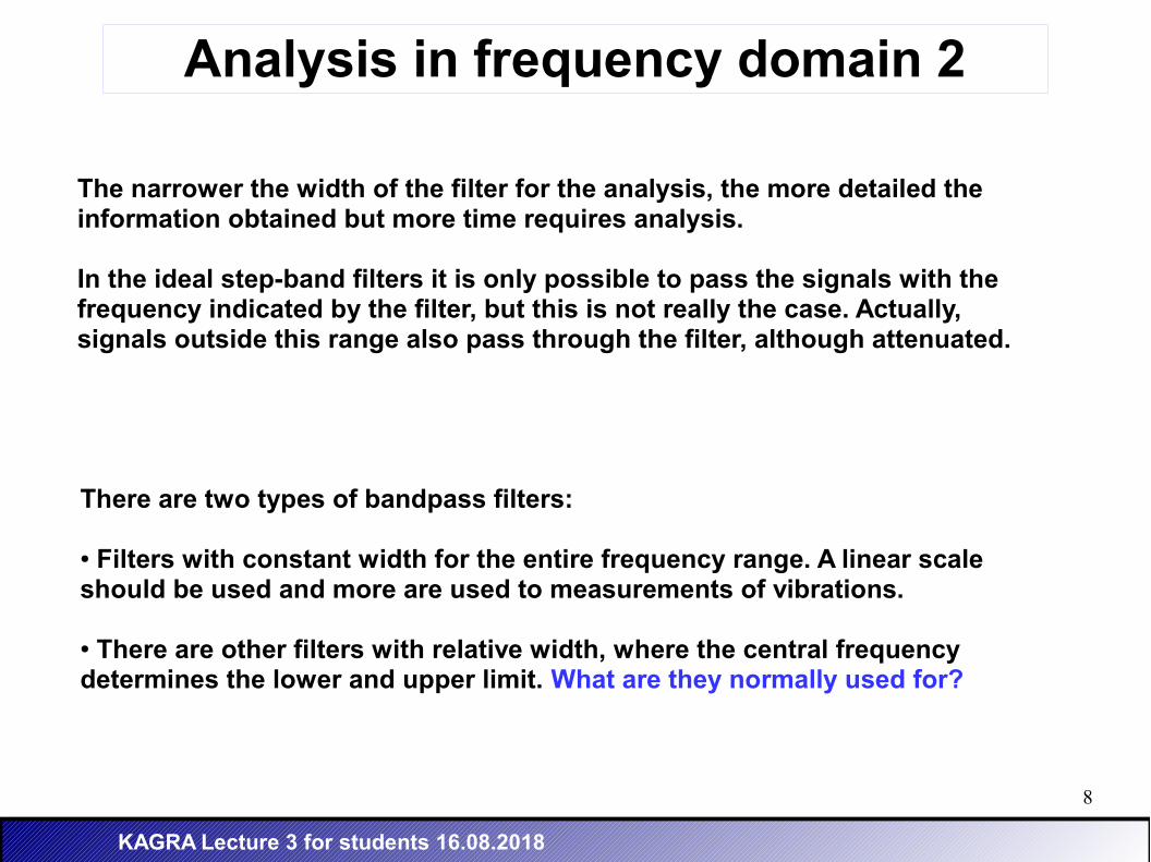
The narrower the width of the filter for the analysis, the more detailed the information obtained but more time requires analysis.

In the ideal step-band filters it is only possible to pass the signals with the frequency indicated by the filter, but this is not really the case. Actually, signals outside this range also pass through the filter, although attenuated.

There are two types of bandpass filters:

● Filters with constant width for the entire frequency range. A linear scale should be used and more are used to measurements of vibrations.

● There are other filters with relative width, where the central frequency determines the lower and upper limit. What are they normally used for?

9



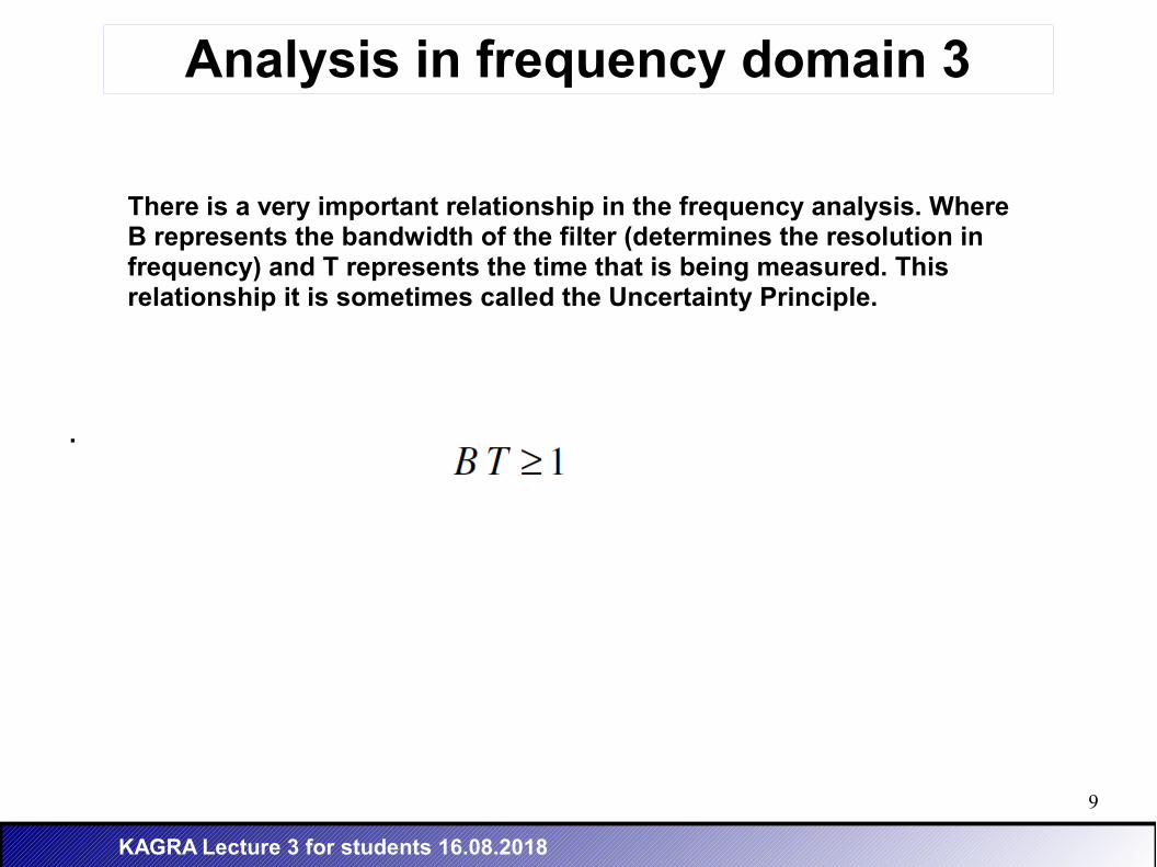
There is a very important relationship in the frequency analysis. Where B represents the bandwidth of the filter (determines the resolution in frequency) and T represents the time that is being measured. This relationship it is sometimes called the Uncertainty Principle.

.

10


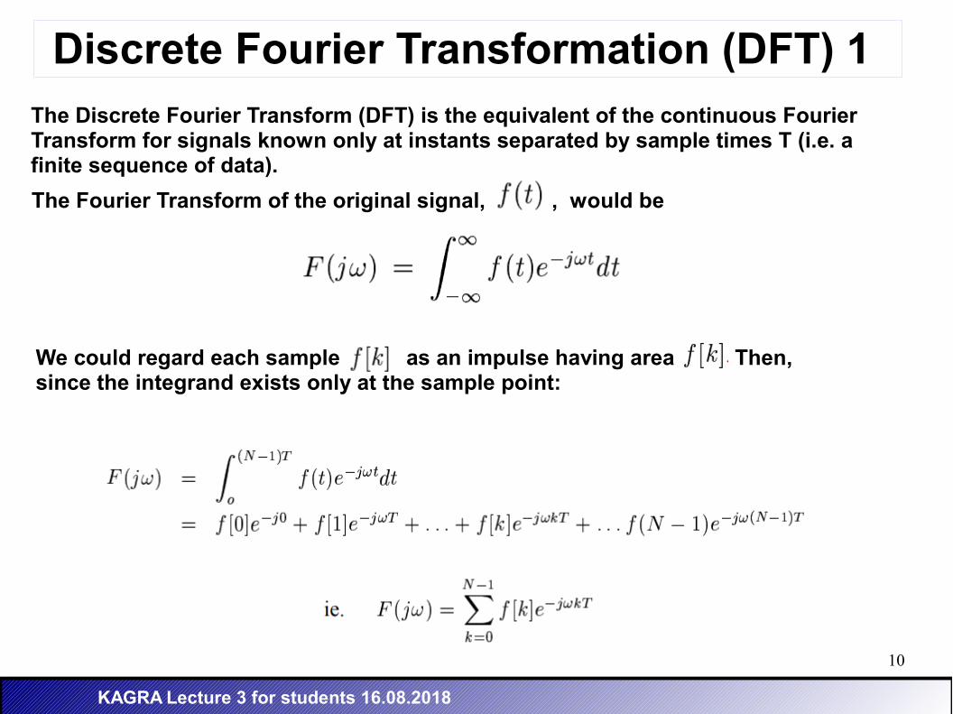
Discrete Fourier Transformation (DFT) 1 The Discrete Fourier Transform (DFT) is the equivalent of the continuous Fourier Transform for signals known only at instants separated by sample times T (i.e. a finite sequence of data).

The Fourier Transform of the original signal, , would be

We could regard each sample as an impulse having area . Then, since the integrand exists only at the sample point:

11


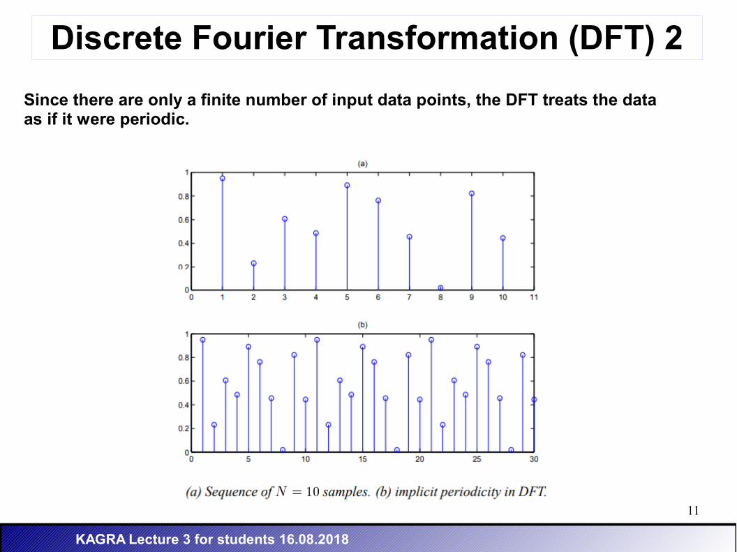
Since there are only a finite number of input data points, the DFT treats the data as if it were periodic.

Discrete Fourier Transformation (DFT) 2

12


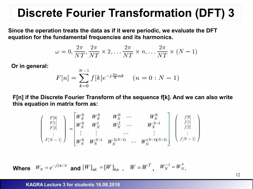
Since the operation treats the data as if it were periodic, we evaluate the DFT equation for the fundamental frequencies and its harmonics.

Discrete Fourier Transformation (DFT) 3

Or in general:

F[n] if the Discrete Fourier Transform of the sequence f[k]. And we can also write this equation in matrix form as:

Where and , , .

13


Fast Fourier Transformation (FFT) 1

Summary:

A Discrete Fourier Transform (DFT) is the name given to the transform of Fourier when applied to a digital (discrete) signal instead of an analog one (continuous).

A Fast Fourier Transform (FFT) is a faster version of the DFT that can be applied when the number of samples of the signal is a power of 2.

The FFT functions are symmetrical, which means that their output includes negative frequencies, that exist purely as mathematical properties of the Fourier Transform.

The first half of the FFT output contains frequencies from 0 Hz to the Nyquist frequency, and the second half is an image with negative frequencies.

14


Fast Fourier Transformation (FFT) 2

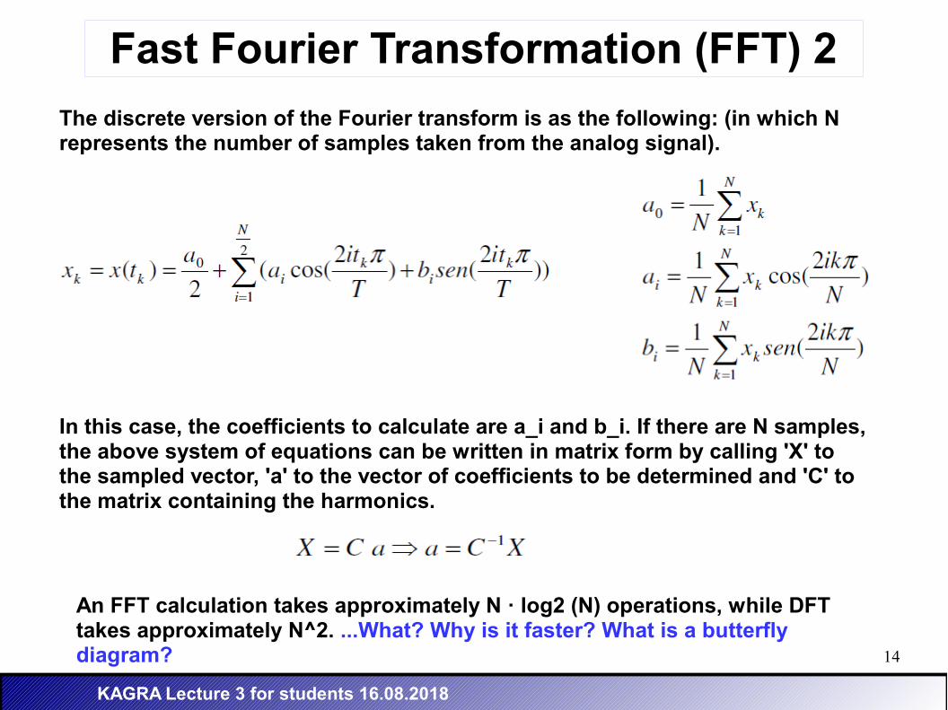
The discrete version of the Fourier transform is as the following: (in which N represents the number of samples taken from the analog signal).

An FFT calculation takes approximately N · log2 (N) operations, while DFT takes approximately N^2. ...What? Why is it faster? What is a butterfly diagram?

In this case, the coefficients to calculate are a_i and b_i. If there are N samples, the above system of equations can be written in matrix form by calling 'X' to the sampled vector, 'a' to the vector of coefficients to be determined and 'C' to the matrix containing the harmonics.

15


Sampling Theorem

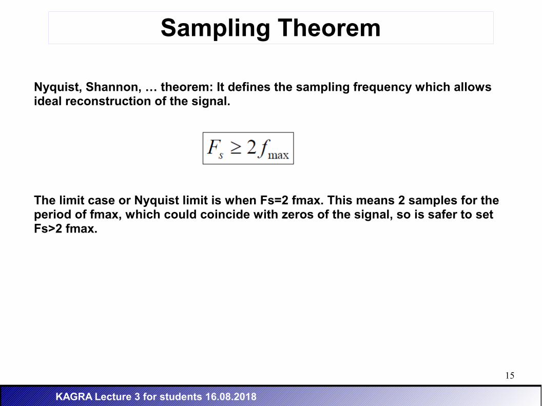
Nyquist, Shannon, … theorem: It defines the sampling frequency which allows ideal reconstruction of the signal.

The limit case or Nyquist limit is when Fs=2 fmax. This means 2 samples for the period of fmax, which could coincide with zeros of the signal, so is safer to set Fs>2 fmax.

16


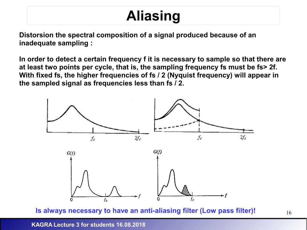
AliasingDistorsion the spectral composition of a signal produced because of an inadequate sampling :

In order to detect a certain frequency f it is necessary to sample so that there are at least two points per cycle, that is, the sampling frequency fs must be fs> 2f. With fixed fs, the higher frequencies of fs / 2 (Nyquist frequency) will appear in the sampled signal as frequencies less than fs / 2.

Is always necessary to have an anti-aliasing filter (Low pass filter)!

17


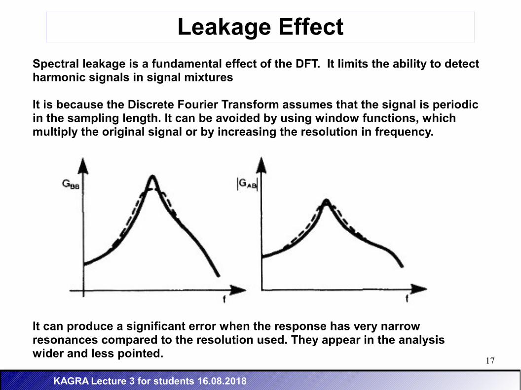
Leakage EffectSpectral leakage is a fundamental effect of the DFT. It limits the ability to detect harmonic signals in signal mixtures

It is because the Discrete Fourier Transform assumes that the signal is periodic in the sampling length. It can be avoided by using window functions, which multiply the original signal or by increasing the resolution in frequency.

It can produce a significant error when the response has very narrow resonances compared to the resolution used. They appear in the analysis wider and less pointed.

18


Transfer functions 1

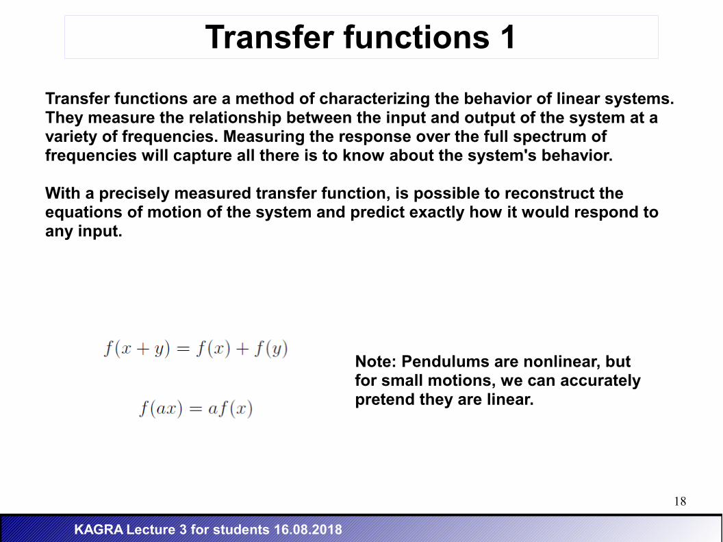
Transfer functions are a method of characterizing the behavior of linear systems. They measure the relationship between the input and output of the system at a variety of frequencies. Measuring the response over the full spectrum of frequencies will capture all there is to know about the system's behavior.

With a precisely measured transfer function, is possible to reconstruct the equations of motion of the system and predict exactly how it would respond to any input.

Note: Pendulums are nonlinear, but for small motions, we can accurately pretend they are linear.

19



When a system first receives an input excitation there are usually some temporary transient behaviors, related to motion at the resonance frequencies. This transient response will decay due to the natural damping of the system leaving behind only the forced response at the frequency of the input. The time after the transient response decays is called the steady state.

The simplest way to measure a transfer function is to inject a force into the suspension in the form of a sine wave at some frequency and amplitude. After some amount of time the suspension responds by moving at this same frequency. From this response we can get the amplitude and phase (or 'time-delay'). Often, the suspension will not respond immediately to the input so the response sine wave will be shifted out of phase with the input sine wave. This time delay is typically measured in units of degrees.

20



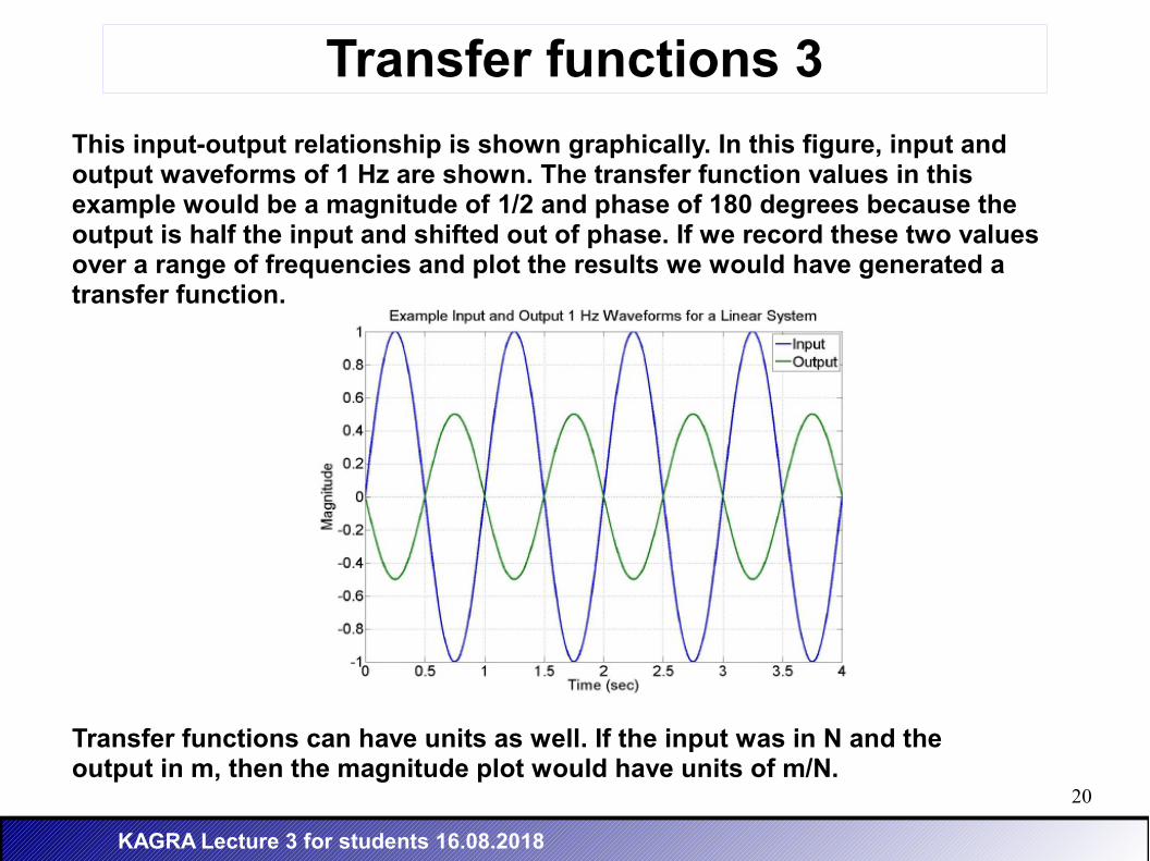
This input-output relationship is shown graphically. In this figure, input and output waveforms of 1 Hz are shown. The transfer function values in this example would be a magnitude of 1/2 and phase of 180 degrees because the output is half the input and shifted out of phase. If we record these two values over a range of frequencies and plot the results we would have generated a transfer function.

Transfer functions can have units as well. If the input was in N and the output in m, then the magnitude plot would have units of m/N.

21



This method of measuring a transfer function is called a swept-sine or stepped-sine because individual sine waves are tested in increments of frequency. It has the advantage of being very precise, but slow.

A faster method is to inject an input that has a spectrum of frequencies. The transfer function is then the spectrum of the output divided by the spectrum of the input. Since each signal is spread over an entire space of frequencies the measurement is less precise because each frequency has a weaker signal and any noise present becomes more signicant.

One can limit the range of frequencies injected to a limited band to improve the accuracy (As the bandwidth goes to zero reconstructs the swept-sine case). Also, one can repeat this measurement a number of times and then average all the results together to get a more accurate measurement. Then you only need to take enough averages to get the precision you need.

Diaggui (DTT) can measure transfer functions using both of these methods.

22


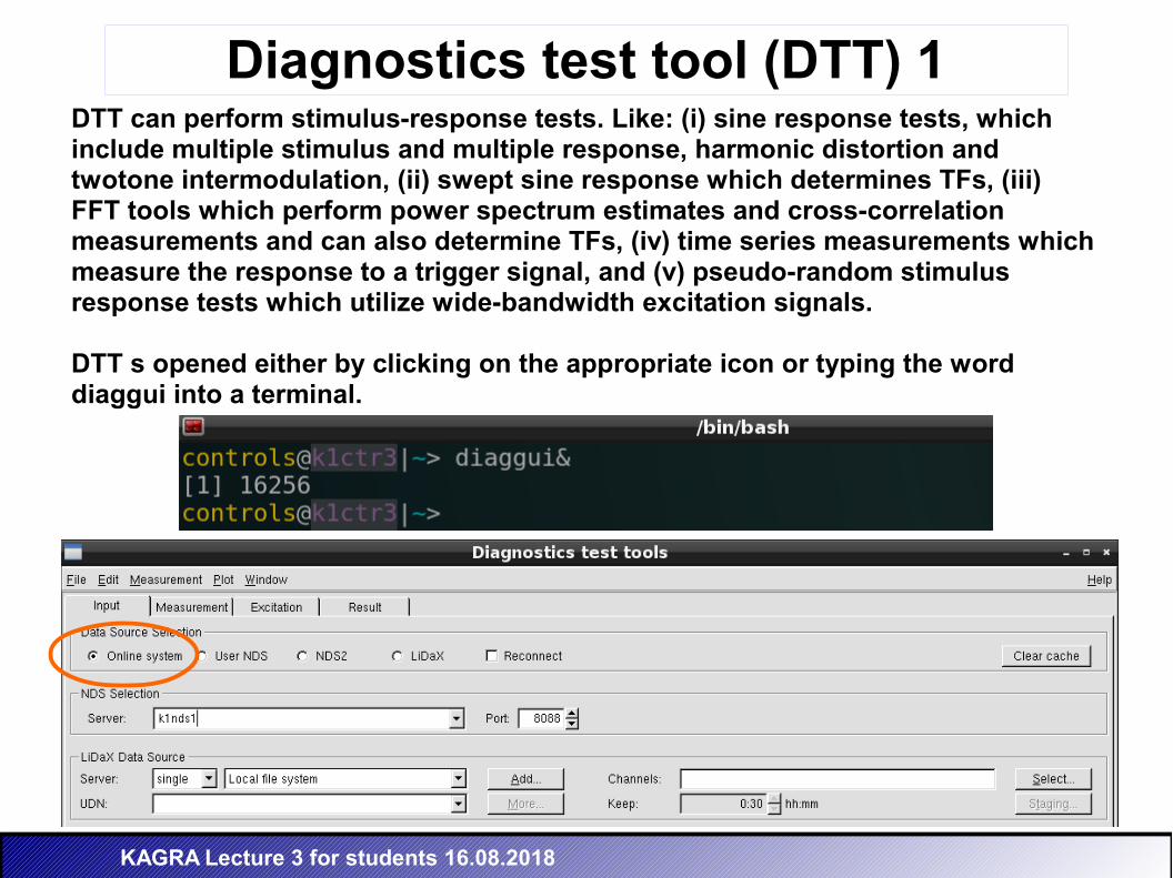
Diagnostics test tool (DTT) 1DTT can perform stimulus-response tests. Like: (i) sine response tests, which include multiple stimulus and multiple response, harmonic distortion and twotone intermodulation, (ii) swept sine response which determines TFs, (iii) FFT tools which perform power spectrum estimates and cross-correlation measurements and can also determine TFs, (iv) time series measurements which measure the response to a trigger signal, and (v) pseudo-random stimulusresponse tests which utilize wide-bandwidth excitation signals.

DTT s opened either by clicking on the appropriate icon or typing the word diaggui into a terminal.

23


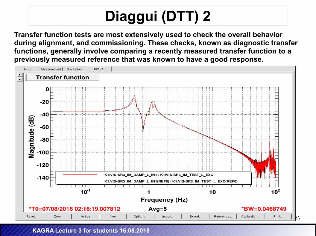
Diaggui (DTT) 2Transfer function tests are most extensively used to check the overall behavior during alignment, and commissioning. These checks, known as diagnostic transfer functions, generally involve comparing a recently measured transfer function to a previously measured reference that was known to have a good response.

24


Diaggui (DTT) 3

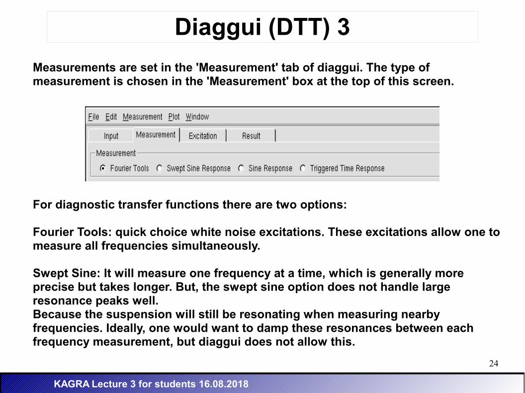
Measurements are set in the 'Measurement' tab of diaggui. The type of measurement is chosen in the 'Measurement' box at the top of this screen.

For diagnostic transfer functions there are two options:

Fourier Tools: quick choice white noise excitations. These excitations allow one to measure all frequencies simultaneously. Swept Sine: It will measure one frequency at a time, which is generally more precise but takes longer. But, the swept sine option does not handle large resonance peaks well. Because the suspension will still be resonating when measuring nearby frequencies. Ideally, one would want to damp these resonances between each frequency measurement, but diaggui does not allow this.

25


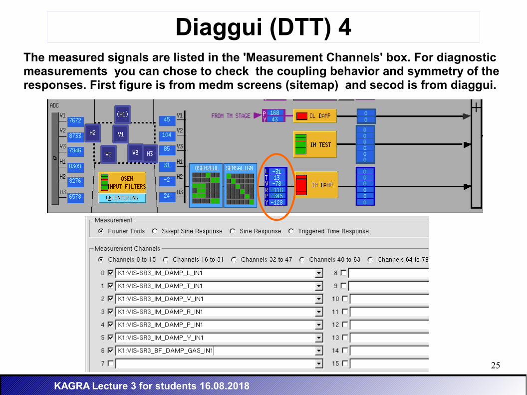
Diaggui (DTT) 4The measured signals are listed in the 'Measurement Channels' box. For diagnostic measurements you can chose to check the coupling behavior and symmetry of the responses. First figure is from medm screens (sitemap) and secod is from diaggui.

26


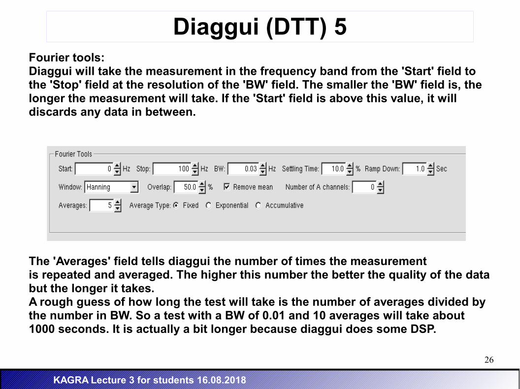
Diaggui (DTT) 5Fourier tools:Diaggui will take the measurement in the frequency band from the 'Start' field to the 'Stop' field at the resolution of the 'BW' field. The smaller the 'BW' field is, the longer the measurement will take. If the 'Start' field is above this value, it will discards any data in between.

The 'Averages' field tells diaggui the number of times the measurementis repeated and averaged. The higher this number the better the quality of the data but the longer it takes. A rough guess of how long the test will take is the number of averages divided by the number in BW. So a test with a BW of 0.01 and 10 averages will take about 1000 seconds. It is actually a bit longer because diaggui does some DSP.

27


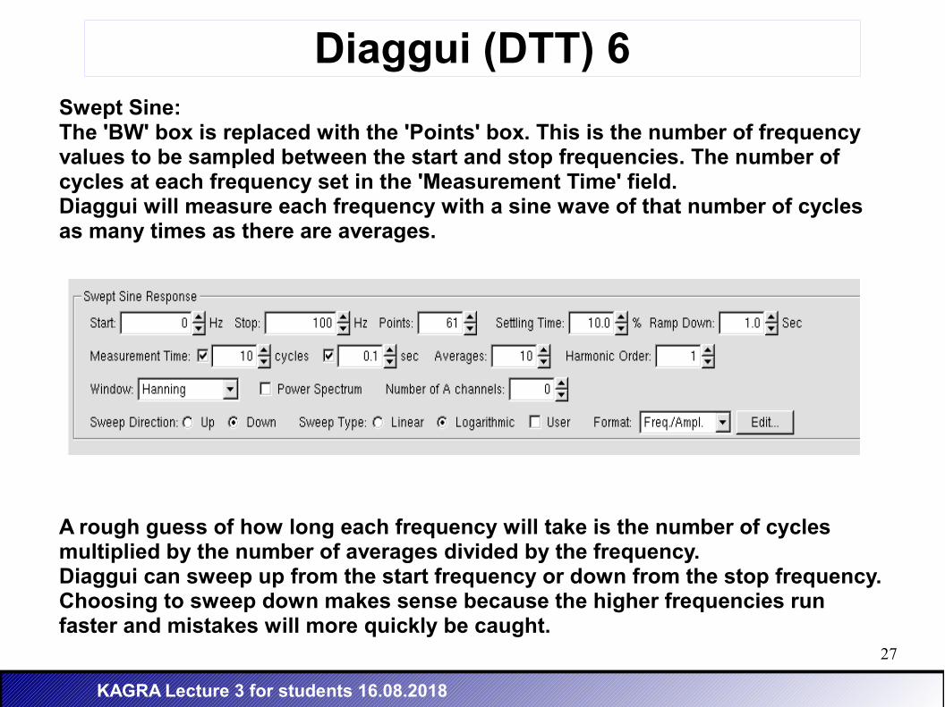
Diaggui (DTT) 6Swept Sine:The 'BW' box is replaced with the 'Points' box. This is the number of frequency values to be sampled between the start and stop frequencies. The number of cycles at each frequency set in the 'Measurement Time' field. Diaggui will measure each frequency with a sine wave of that number of cycles as many times as there are averages.

A rough guess of how long each frequency will take is the number of cycles multiplied by the number of averages divided by the frequency. Diaggui can sweep up from the start frequency or down from the stop frequency. Choosing to sweep down makes sense because the higher frequencies run faster and mistakes will more quickly be caught.

28


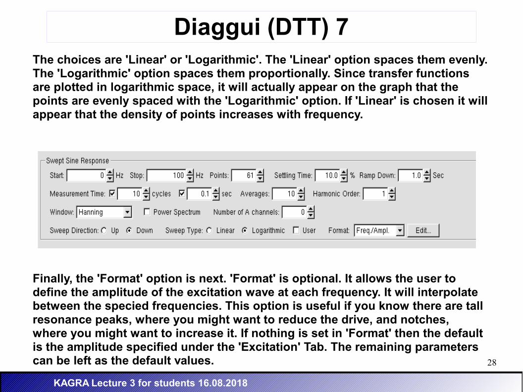
Diaggui (DTT) 7The choices are 'Linear' or 'Logarithmic'. The 'Linear' option spaces them evenly. The 'Logarithmic' option spaces them proportionally. Since transfer functions are plotted in logarithmic space, it will actually appear on the graph that the points are evenly spaced with the 'Logarithmic' option. If 'Linear' is chosen it will appear that the density of points increases with frequency.

Finally, the 'Format' option is next. 'Format' is optional. It allows the user to define the amplitude of the excitation wave at each frequency. It will interpolate between the specied frequencies. This option is useful if you know there are tall resonance peaks, where you might want to reduce the drive, and notches, where you might want to increase it. If nothing is set in 'Format' then the default is the amplitude specified under the 'Excitation' Tab. The remaining parameters can be left as the default values.

29


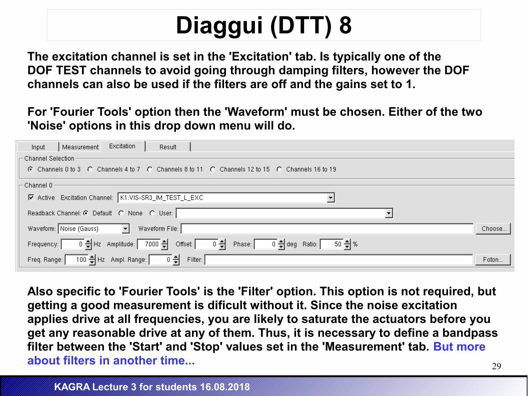
Diaggui (DTT) 8The excitation channel is set in the 'Excitation' tab. Is typically one of theDOF TEST channels to avoid going through damping filters, however the DOF channels can also be used if the filters are off and the gains set to 1.

For 'Fourier Tools' option then the 'Waveform' must be chosen. Either of the two 'Noise' options in this drop down menu will do.

Also specific to 'Fourier Tools' is the 'Filter' option. This option is not required, but getting a good measurement is dificult without it. Since the noise excitation applies drive at all frequencies, you are likely to saturate the actuators before you get any reasonable drive at any of them. Thus, it is necessary to define a bandpass filter between the 'Start' and 'Stop' values set in the 'Measurement' tab. But more about filters in another time...

30


Diaggui (DTT) 9

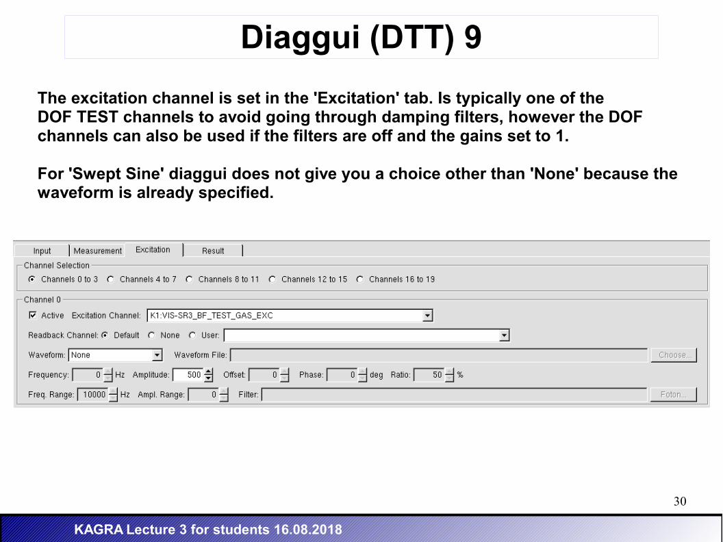
The excitation channel is set in the 'Excitation' tab. Is typically one of theDOF TEST channels to avoid going through damping filters, however the DOF channels can also be used if the filters are off and the gains set to 1.

For 'Swept Sine' diaggui does not give you a choice other than 'None' because the waveform is already specified.

31


Diaggui (DTT) 10

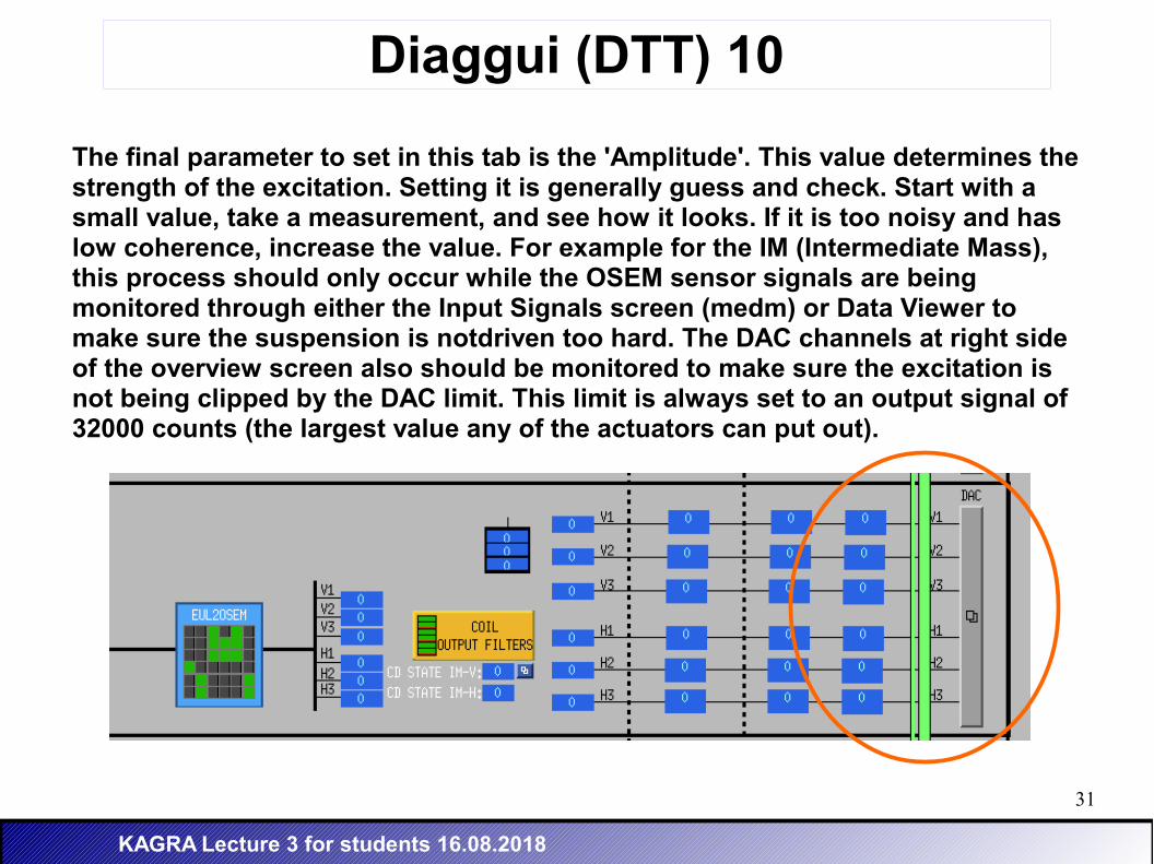
The final parameter to set in this tab is the 'Amplitude'. This value determines the strength of the excitation. Setting it is generally guess and check. Start with a small value, take a measurement, and see how it looks. If it is too noisy and has low coherence, increase the value. For example for the IM (Intermediate Mass), this process should only occur while the OSEM sensor signals are being monitored through either the Input Signals screen (medm) or Data Viewer to make sure the suspension is notdriven too hard. The DAC channels at right side of the overview screen also should be monitored to make sure the excitation is not being clipped by the DAC limit. This limit is always set to an output signal of 32000 counts (the largest value any of the actuators can put out).

32


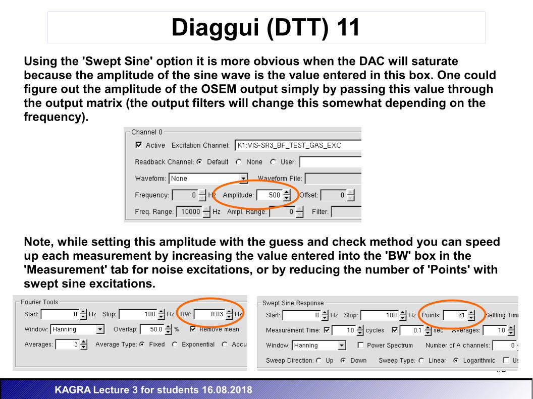
Diaggui (DTT) 11Using the 'Swept Sine' option it is more obvious when the DAC will saturate because the amplitude of the sine wave is the value entered in this box. One could figure out the amplitude of the OSEM output simply by passing this value through the output matrix (the output filters will change this somewhat depending on the frequency).

Note, while setting this amplitude with the guess and check method you can speed up each measurement by increasing the value entered into the 'BW' box in the 'Measurement' tab for noise excitations, or by reducing the number of 'Points' with swept sine excitations.

33


Diaggui (DTT) 12

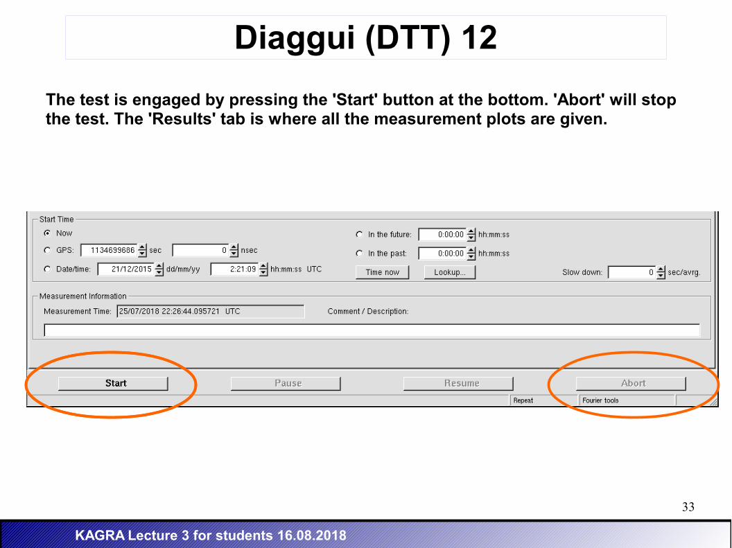
The test is engaged by pressing the 'Start' button at the bottom. 'Abort' will stop the test. The 'Results' tab is where all the measurement plots are given.

34


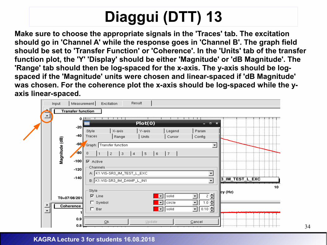
Diaggui (DTT) 13Make sure to choose the appropriate signals in the 'Traces' tab. The excitation should go in 'Channel A' while the response goes in 'Channel B'. The graph field should be set to 'Transfer Function' or 'Coherence'. In the 'Units' tab of the transfer function plot, the 'Y' 'Display' should be either 'Magnitude' or 'dB Magnitude'. The 'Range' tab should then be log-spaced for the x-axis. The y-axis should be log-spaced if the 'Magnitude' units were chosen and linear-spaced if 'dB Magnitude' was chosen. For the coherence plot the x-axis should be log-spaced while the y-axis linear-spaced.

35


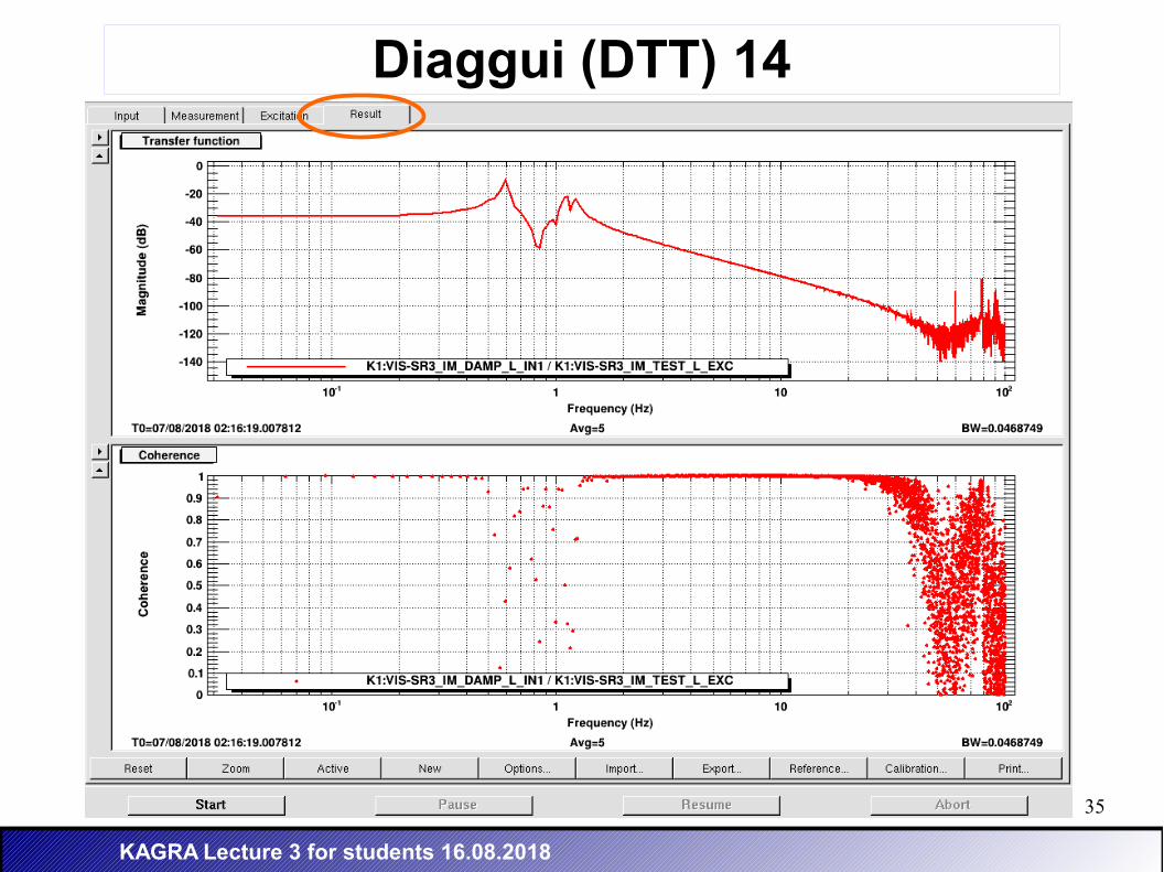
Diaggui (DTT) 14

36


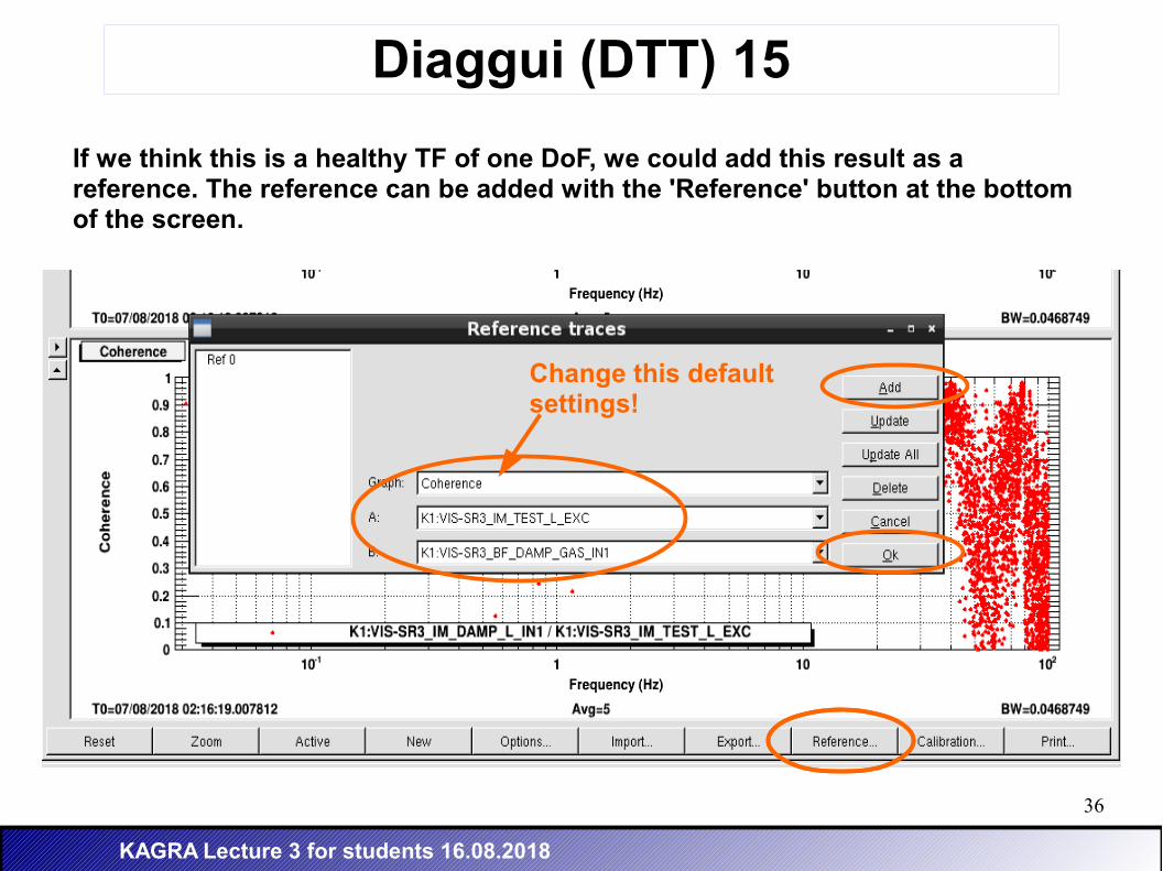
Diaggui (DTT) 15

If we think this is a healthy TF of one DoF, we could add this result as a reference. The reference can be added with the 'Reference' button at the bottom of the screen.

Change this default settings!

37


Tasks

(1) Why is it faster the FFT? What is butterfly diagram of FFT?

(2) What does the coherence mean in a TF measurement?

(3) Take TF using fourier tools for the BF, SF and F0 of the BS. Include the amplitude, phase and coherence. Do not use any template and estimate the amplitude necessary of the excitation for that DoF using Data Viewer. As we discussed before, this is generally guess and check. Start with a small value, take a measurement, and see how it looks. If it is too noisy and has low coherence, increase the value.

38


Next Lectures

● GAS Filters details. ◯● FFTs, windowing, aliasing,

leakage, … ◯

● Use of diaggui. ◯

● Transfer Functions (TF).◯● OSEMs details by Enzo and

Oplev details by Terrence.

● Payload modelling by Kozu.

● Inverted pendulum modelling.

● Explanation of Medm screens in general for VIS.

● Explanation about OSEMs.

● RTM implementation (Simulink).

Plan for next weeks: Suggestions for next weeks?

39


Bibliography

●DFT/FFT Transforms and Applications.

● Diagnostics Test Software by D. Sigg and P. Fritschel.

● Electronics Setup and testing LIGO by B. Shapiro.

You can get these and more documents from the KAGRA wiki page:

http://gwwiki.icrr.u-tokyo.ac.jp/JGWwiki/KAGRA/Subgroups/VIS/Introduction

Documents

Concepts of DSP (Digital Signal Processing) and use of DTT