Journal of Coastal Research 21 2 307–322 West Palm Beach, Florida March 2005

Concepts in Sediment Budgets Julie Dean Rosati

U.S. Army Corps of Engineers Engineer Research Development Center Coastal and Hydraulics Laboratory Vicksburg, MS 39180-6199, U.S.A.

ABSTRACT

ROSATI, J.D., 2005, Concepts in sediment budgets. Journal of Coastal Research, 21(2), 307–322. West Palm Beach (Florida), ISSN 0749-0208.

The sediment budget is fundamental in coastal science and engineering. Budgets allow estimates to be made of the volume or volume rate of sediment entering and exiting a defined region of the coast and the surplus or deficit remaining in that region. Sediment budgets have been regularly employed with variations in approaches to determine the sources and sinks through application of the primary conservation of mass equation. Historically, sediment budgets have been constructed and displayed on paper or maps. Challenges in constructing a sediment budget include deter­mining the appropriate boundaries of the budget and interior cells; defining the possible range of sediment transport pathways, and the relative magnitude of each; representing the uncertainty associated with values and assumptions in the budget; and testing the sensitivity of the series of budgets to variations in the unknown and temporally-changing values. These challenges are usually addressed by representing a series of budget alternatives that are ultimately drawn on paper, maps, or graphs. Applications of the methodology include detailed local-scale sediment budgets, such as for an inlet or beach fill project, and large-scale sediment budgets for the region surrounding the study area. The local-scale budget has calculation cells representing features on the order of 10s to 100s of meters, and it must be shown separately from the regional sediment budget, with cells ranging from 100s of meters to kilometers.

This paper reviews commonly applied sediment budget concepts and introduces new considerations intended to make the sediment budget process more reliable, streamlined, and understandable. The need for both local and regional sediment budgets is discussed, and the utility of combining, or collapsing, cells is shown to be beneficial for local budgets within a regional system. Collapsing all cells within the budget creates a ‘‘macrobudget,’’ which can be applied to check for overall balance of values. An automated means of changing the magnitude of terms, while main­taining the same dependency on other values within the sediment budget, is presented. Finally, the need for and method of tracking uncertainty within the sediment budget, and a means for conducting sensitivity analyses, are discussed. These new concepts are demonstrated within the Sediment Budget Analysis System with an application for Long Island, New York, and Ocean City Inlet, Maryland.

ADDITIONAL INDEX WORDS: Uncertainty, sensitivity testing, Long Island, New York, Ocean City Inlet, Maryland, regional scale, computer program, beaches.

INTRODUCTION

Sediment budgets are regularly created in coastal engi­neering and science studies to develop understanding of the sediment sources, sinks, transport pathways and magnitudes for a selected region of coast and within a defined period of time. The sediment budget is a balance of volumes (or volume rates of change) for sediments entering (source) and leaving (sink) a selected region of coast, and the resulting erosion or accretion in the coastal area under consideration. The sedi­ment budget may be constructed to represent short-term con­ditions, such as for a particular season of the year, to longer time periods representing a particular historical time period or existing conditions at the site. Once the sediment budget has been developed, values in the budget may be altered to explore possible erosional or accretionary aspects of a pro­posed engineering project, or variations in assumed terms. Sediment budgets are a fundamental tool for project man-

DOI: 10.2112/02-475A.1 received 10 October 2002; accepted in revi­sion 12 July 2003.

agement, and they often serve as a common framework for discussions with colleagues and sponsors involved in a study.

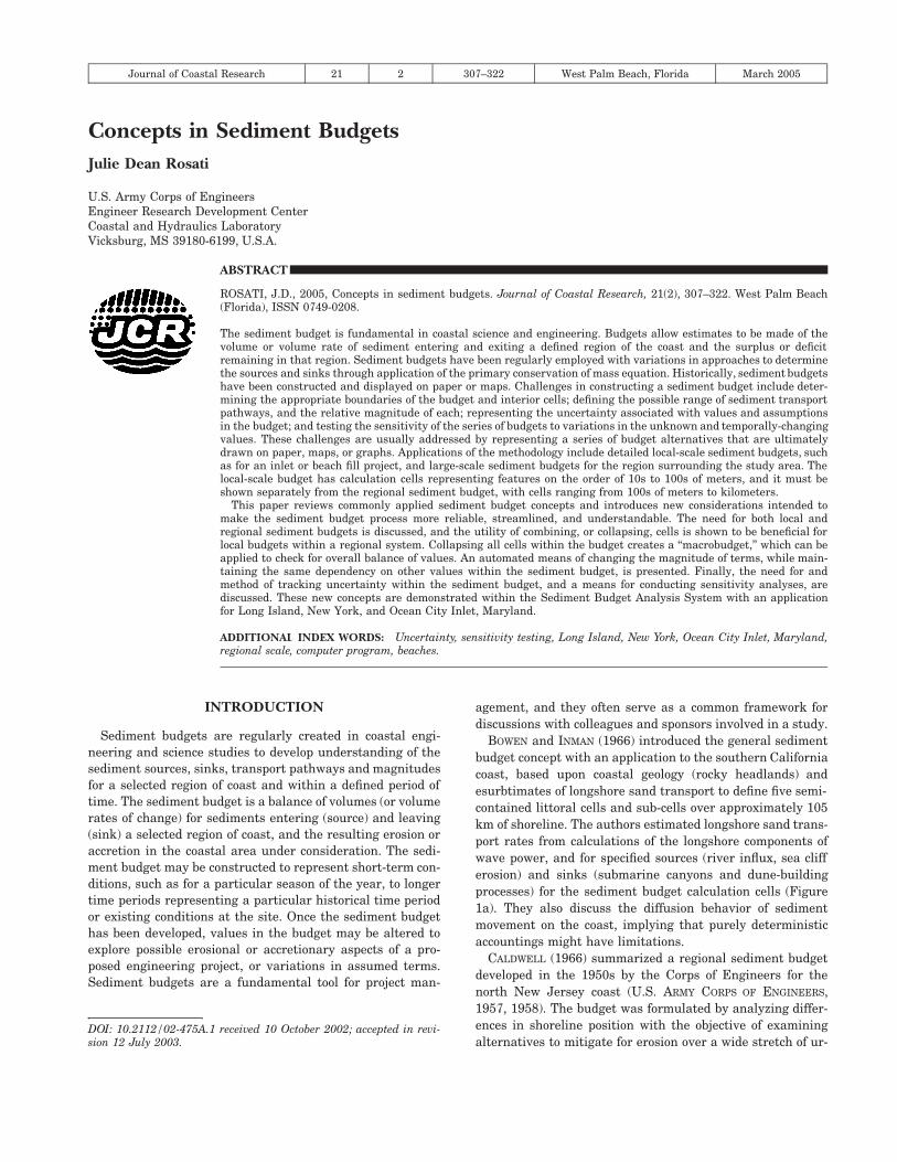
BOWEN and INMAN (1966) introduced the general sediment budget concept with an application to the southern California coast, based upon coastal geology (rocky headlands) and esurbtimates of longshore sand transport to define five semi-contained littoral cells and sub-cells over approximately 105 km of shoreline. The authors estimated longshore sand trans­port rates from calculations of the longshore components of wave power, and for specified sources (river influx, sea cliff erosion) and sinks (submarine canyons and dune-building processes) for the sediment budget calculation cells (Figure 1a). They also discuss the diffusion behavior of sediment movement on the coast, implying that purely deterministic accountings might have limitations.

CALDWELL (1966) summarized a regional sediment budget developed in the 1950s by the Corps of Engineers for the north New Jersey coast (U.S. ARMY CORPS OF ENGINEERS, 1957, 1958). The budget was formulated by analyzing differ­ences in shoreline position with the objective of examining alternatives to mitigate for erosion over a wide stretch of ur­

308 Rosati

Figure 1. Early sediment budgets (a) Southern California sediment bud­get (adapted from Bowen and Inman 1966), (b) North New Jersey sedi­ment budget (adapted from Caldwell 1966).

banized and semiurbanized beach. This study deduced the existence of a regional divergent nodal area in net longshore transport direction at Mantoloking, located just north of Do­ver Township. Net longshore transport to the north increased with distance north from Mantoloking because of the wave

sheltering by Long Island, New York. The budget covered average annual net and gross longshore sand transport rates for this 190-km reach, including ten inlets, over time inter­vals of 50 to 115 years. Both the magnitudes and directions of transport, including location of the nodal area, are still considered to be valid (Figure 1b).

Today, sediment budgets are a fundamental element of coastal sediment processes studies encompassing many ap­plications (KOMAR, 1998). Budgets typically start from docu­mented accretion and erosion to estimate other contributions with higher uncertainty. Budgets serve as a common frame­work to evaluate alternative project designs, develop an un­derstanding of sediment transport pathways through time, or estimate future rates of sediment accretion or erosion. This paper reviews sediment budget concepts and introduces new considerations intended to streamline the sediment budget evaluation and presentation process. Estimation of uncer­tainty in sediment budgets is considered a central element of a modern treatment. The state of personal computer tech­nology has allowed automation of many convenient, if not essential, features of the new concepts. Basic and new sedi­ment budget methods are demonstrated with applications for Long Island, New York and Ocean City Inlet, Maryland.

REVIEW OF SEDIMENT BUDGET CONCEPTS

Theory and Definitions

A sediment budget is a tally of sediment gains and losses, or sources and sinks, within a specified control volume (or cell), or in a series of connecting calculation cells, over a given time. As with any accounting system, the algebraic difference between sediment sources and sinks in each cell, hence for the entire sediment budget, must equal the rate of change in sediment volume occurring within that region, accounting for possible engineering activities. Expressed in terms of vari­ables consistent as volume or as volumetric rate of change, the sediment budget equation is,

2 Q - 2 Q - LV + P - R = Residual (1)source sink

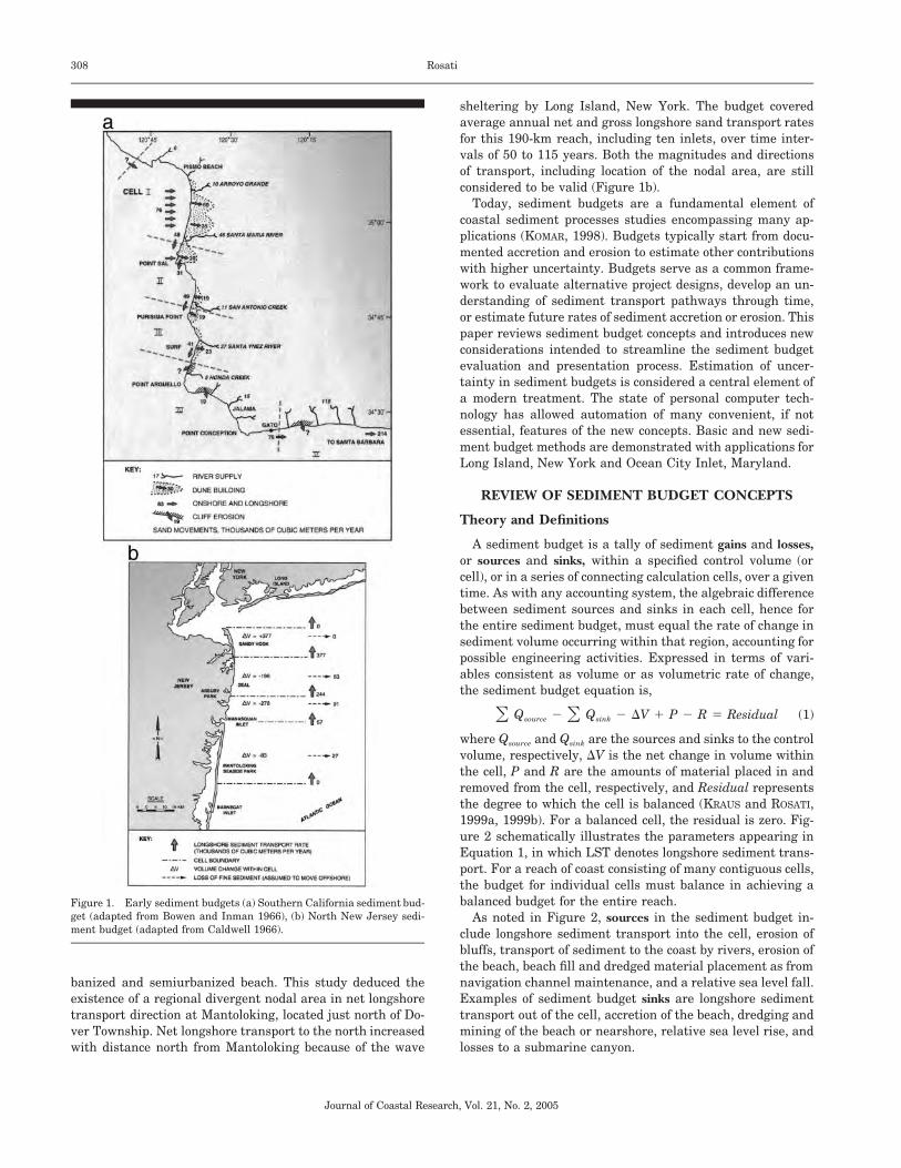
where Qsource and Qsink are the sources and sinks to the control volume, respectively, LV is the net change in volume within the cell, P and R are the amounts of material placed in and removed from the cell, respectively, and Residual represents the degree to which the cell is balanced (KRAUS and ROSATI, 1999a, 1999b). For a balanced cell, the residual is zero. Fig­ure 2 schematically illustrates the parameters appearing in Equation 1, in which LST denotes longshore sediment trans­port. For a reach of coast consisting of many contiguous cells, the budget for individual cells must balance in achieving a balanced budget for the entire reach.

As noted in Figure 2, sources in the sediment budget in­clude longshore sediment transport into the cell, erosion of bluffs, transport of sediment to the coast by rivers, erosion of the beach, beach fill and dredged material placement as from navigation channel maintenance, and a relative sea level fall. Examples of sediment budget sinks are longshore sediment transport out of the cell, accretion of the beach, dredging and mining of the beach or nearshore, relative sea level rise, and losses to a submarine canyon.

Journal of Coastal Research, Vol. 21, No. 2, 2005

309 Concepts in Sediment Budgets

Figure 2. Sediment budget parameters as may enter Equation (1).

Longshore transport rates may be defined as left- and right-directed or as net and gross. The net longshore trans­port rate is defined as the difference between the right-di­rected and left-directed littoral transport over a specified time interval for a seaward-facing observer,

Qnet = QR - QL (2)

in which both the leftward-directed transport QL and right­ward-directed transport QR are taken as positive. The gross longshore transport rate is defined as the sum of the right-directed and left-directed transport rates over a specified time interval for a seaward-facing observer,

Qgross = QR + QL (3)

An inlet channel may capture much of the left- and right-directed components of the longshore transport, and the inlet system may bypass left- and right-directed longshore trans­port. Thus, knowledge of the net and gross transport rates, as well as pathways of sediment transport for left- and right-directed dominance (as might occur during seasons of net transport reversal), are required to accurately represent transport within the vicinity of inlets (BODGE, 1993). The net or predominant direction of longshore sediment transport at an inlet or at a groin or jetty can usually be inferred by the asymmetry in geomorphology at the site (CARR and KRAUS, 2001). The asymmetry can be related to the ratio of net to gross longshore transport Qnet/Qgross which varies from zero (balanced left- and right-directed longshore transport, hence near-symmetrical morphology) to unity (unidirectional long-shore transport).

Estimating Values in the Sediment Budget

Overview. Several approaches have been developed that ap­ply a form of Equation (1). Generally, these methods estimate a likely range of values for the best-known quantities and solve for the lesser-known terms. Volume change data, and removal and placement records usually provide the founda­tion for the sediment budget. Then, a range of ‘‘accepted’’ longshore transport rates and a range in relative magnitude of other fluxes are applied to solve the budget. Imbalance of the equation is addressed by varying these parameters, and other terms with great uncertainty, such as offshore losses

and wind-blown transport, and uncertainty in the values of the best-known quantities.

Conceptual Budget. DOLAN et al. (1987) and KANA and STE­

VENS (1992) discuss a ‘‘conceptual sediment budget,’’ which they recommend developing in the planning stage prior to making detailed calculations. The conceptual sediment bud­get is a qualitative model giving a regional perspective of beach and inlet processes, containing the effects of offshore bathymetry (particularly shoals and, therefore, wave-driven sources and sinks), and incorporating natural morphologic in­dicators of net (and gross) sand transport. The conceptual model may be put together in part by adopting sediment bud­gets developed for other sites in similar settings, and incor­porates all sediment sinks, sources, and pathways. The con­ceptual model is developed initially, perhaps based upon a reconnaissance study at the site as part of the initial data set. Once the conceptual sediment budget has been complet­ed, data are assimilated to validate the conceptual model rather than to develop the model.

Delineating Sediment Budget Cells. Sediment budget cal­culation cells or ‘‘control volumes’’ define the boundaries for each sediment budget calculation and denote the existence of a complete self-contained sediment budget within its bound­aries (DOLAN et al., 1987). Cells are defined by geologic con­trols, available data resolution, coastal structures, knowledge of the site, and to isolate known quantities or the quantity of interest. From one to a nearly unlimited number of cells may be defined using one or more of these means to characterize the sediment transport regime of a region. BOWEN and INMAN

(1966) introduced the concept of littoral cells (INMAN and FRAUTSCHY, 1966) within a sediment budget. The southern California coast lends itself to this concept, with evident sources (river influx, sea cliff erosion), sinks (submarine can­yons), and coastal geology (rocky headlands) defining semi-contained littoral cells and subcells (KOMAR, 1996, 1998). A littoral cell can also be defined to represent a region bounded by assumed or better known transport conditions, or by en­gineered or natural features such as by a long jetty or by the average location of a nodal region (zone in which Qnet � 0) in net longshore transport direction.

Defining Sediment Budget Pathways. Sediment budget pathways specify the significant transport transfers between cells within a sediment budget. Pathways can be estimated through knowledge of the site, by examining aerial photo­graphs, field observation of drogue or dye movement, through interpretation of engineering activities such as channel dredging and evolution of beach fill, and mapping of bedforms on the sea floor using side scan sonar (e.g., BLACK and HEALY

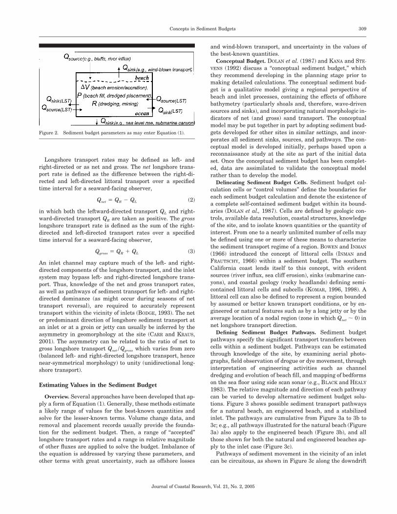
1983). The relative magnitude and direction of each pathway can be varied to develop alternative sediment budget solu­tions. Figure 3 shows possible sediment transport pathways for a natural beach, an engineered beach, and a stabilized inlet. The pathways are cumulative from Figure 3a to 3b to 3c; e.g., all pathways illustrated for the natural beach (Figure 3a) also apply to the engineered beach (Figure 3b), and all those shown for both the natural and engineered beaches ap­ply to the inlet case (Figure 3c).

Pathways of sediment movement in the vicinity of an inlet can be circuitous, as shown in Figure 3c along the downdrift

Journal of Coastal Research, Vol. 21, No. 2, 2005

310 Rosati

Figure 3. Possible sediment transport pathways for different types of coastal regions (a) Natural beach, (b) Engineered beach, (c) Inlet and ad­jacent beaches (Note: All pathways illustrated for the natural beach (a) also apply to the engineered beach (b), and all those shown for both the natural and engineered beaches apply to the inlet case (c)).

beach. Thus, equations describing the sediment budget for regions directly adjacent to the inlet are not unique (i.e., dif­ferent formulations are possible). For natural and engineered beaches (Figures 3a and 3b), determining the magnitude of sediment transport may present a challenge, but the path­ways are relatively simple to define. An inlet channel has the potential to capture the left- and right-directed components of the gross longshore transport of sediment, and the inlet system may bypass left- and right-directed longshore trans­port. Thus, knowledge of the net and gross transport rates, as well as the potential behavior of the inlet with respect to the transport pathways, may be required to correctly repre­sent transport conditions within the vicinity of inlets, as em­phasized by BODGE (1993).

BODGE (1999) presents an algebraic method with which a range of sediment budget solutions can be developed to nu­merically bound and describe sediment transport pathways at inlets. The method incorporates examination of the sedi­ment budget based on a range in the following variables: net and gross longshore sediment transport rates, permeability of jetties to sediment transport, natural bypassing rate from both the updrift and downdrift beaches, and the magnitude of local inlet-induced transport on both the updrift and down-drift beaches. The method also accounts for riverine input, dredging and placement, and mechanical bypassing. Because ranges of values are involved, the final result is a family of solutions that balance the sediment budget. One or several of these solutions may be selected to represent typical sedi­ment transport conditions at the site. Viewing the area de­fined by the ranges allows one to judge, at least subjectively, the reasonability of selecting various values to represent a particular budget.

Volume Change, Removal, and Placement. Volume change, removal and placement of dredged material or beach fill must be included in the sediment budget if pertinent to the time period being analyzed. Volume change magnitudes and rates may be estimated for each cell of the sediment budget using shoreline position data, beach profile data, bathymetric change data, or shoreline change rates. Alternatively, Equa­tion (1) can be applied with estimates of longshore transport rates to solve for the net volume change within each cell. Because many sediment budgets are formulated based on his­torical data, the dredging and placement methods used at the time the data were collected must be known. The following is summarized from KRAUS and ROSATI (1999a, 1999b).

Estimating the actual volume dredged and subsequent placement of the material is dependent on the type of equip­ment used, time frame of removal and placement, and type of material. For example, a hopper dredge may have been filled to capacity while allowing overflow of fine sediments, which theoretically would be transported away from an inlet channel by tidal and other currents. In this situation, consid­eration should be given to the possibility that some littoral material may not have been included in the dredging esti­mates, or potentially that the material was rehandled if it settled within the channel. The period of the dredging cycle must also be considered. If the dredging occurred over several months, seasons, or years, a dredging quantity based on pre­dredging and post-dredging bathymetry surveys could rep-

Journal of Coastal Research, Vol. 21, No. 2, 2005

�

311 Concepts in Sediment Budgets

resent additional shoaling of the channel after the initial dredging cycle. The type of material dredged and placed may alter the estimate of the true volume: fine sediments may be suspended during nearshore placement, and thereby overes­timate the quantity introduced to the budget; dredging of or­ganic material may tend to overestimate the volume dredged; and the volume of littoral sediments (e.g., sand, gravel) with­in a mixed material including clays and silts must account for the percentage of non-littoral material in estimations of volumes within the sediment budget.

Practical details may skew an average-annual rate of vol­ume change associated with dredging. For example, some­times overdredging or additional dredging is performed sim­ply because equipment is available. Gross rates of longshore transport inferred from such dredging records will be over­estimates. Similarly, if dredging equipment is damaged in the course of work or must leave a site because of weather, scheduling, or closure of environmental windows, the resul­tant volumes might underestimate the gross rate for that particular period.

One of the more accurate dredging estimates comes from comparison of pre-dredging and post-dredging surveys. The estimates can have significantly different degrees of reliabil­ity and can vary greatly. For example, a dredging contractor is usually paid only for the volume taken out of the design template. If a dredger digs outside the template (whether too deep or to the side of the template), then the reported pay quantity will be less than the volume removed and placed in the disposal area. In calm seas, the reported pay quantity may be only slightly greater than the pay quantity (<+ 20%), whereas in rough seas and intermittent calm and rough seas (when material can move back into the dredging area), the reported quantity might be double the pay quantity ( +100%).

Another method for estimating dredged quantity referenc­es the volume of the storage bin or hopper on a dredge. A typical volume is 765 cu m (1,000 cu yd). One method of de­termining the dredged material volume is to fill the hopper, allow the sediments within the hopper to settle (with excess water spilling over the hopper sides), and measure the ver­tical distance from the top of the hopper to the sediment sur­face. The hopper volume can then be calculated with a rela­tively low uncertainty, estimated at ±10% of the total vol­ume.

A third method of volume calculation is to survey the placed material, whether as an offshore mound or as a beach fill. Uncertainty enters through the insitu voids ratio and whether fine sediments or any of the placed material has run off or slumped beyond the construction template. In this method, the contractor is paid based on surveys aimed to demonstrate that the construction template was filled. Typ­ically, more material must be dredged and placed to meet the survey requirement.

Sidecasting of dredged material is occasionally performed. Typically, an average production rate for the dredge is mul­tiplied by the slurry flow and the time the dredge has oper­ated to obtain a volume. Occasionally, a nuclear-density me­ter operates on the sidecasting arm and can more accurately estimate the percentage of sediment in the dredged slurry.

The uncertainty estimate for these methods is expected to be relatively large, perhaps ±30%.

Sometimes the only estimate of dredged volume is the per­mitted quantity or the design quantity specified to meet depth requirements for navigation, and this ‘‘paper’’ quantity may not provide a reliable estimate of the actual volume dredged. Typically, the permitted or design quantity will be exceeded, but the amount of exceedance is unknown.

In summary, dredged volume inaccuracies can enter as (a) uncertainty in the pre-dredging condition; (b) uncertainty in the volume-estimation process; (c) unquantified sediment shoaling that occurs between the pre- and post-dredging sur­veys; (d) failure to include nonpay volume (material removed from side slopes beyond the design channel location and un­intentional overdepth dredging); and (e) changes in bulk den­sity between the site where the volume was measured and the site or budget compartment where the volume is placed.

Fill can be placed either as an authorized shore-protection (beachfill) project or as a beneficial use of dredged material. For an authorized beachfill project, the fill is surveyed in place to ensure that the design cross-section is met along the shore. For a beneficial-uses project, the placed material will typically not be measured in place, and the volume will be estimated as that from the dredging site. In both cases, con­siderations as discussed above for dredged material will ap­ply.

Fluxes. Sand fluxes within the sediment budget may rep­resent, for example, longshore sand transport due to waves and currents; cross-shore transport, perhaps due to storm-induced transport or relative sea level change; riverine input; aeolian transport; and bluff erosion.

The rate of longshore sand transport along a particular beach is a term that is typically varied in Equation (1) to develop alternative sediment budgets. Longshore transport rates may be estimated through local knowledge of the site; history of engineering activities and the subsequent beach response, such as impoundment at a groin or jetty; and cal­culation of the longshore energy flux due to the site’s wave climate.

Sediment-transport fluxes are difficult to define at inlets, even in a relative sense. Flood and ebb currents, combined waves and currents, wave refraction and diffraction over com­plex bathymetry, and engineering activities complicate trans­port rate directions and may increase or decrease their mag­nitudes.

The Longshore Energy Flux sediment budget method in­corporates incident wave climatology, shoreline position and beach profile data, and bathymetry to develop estimates of breaking wave parameters (JARRETT, 1977, 1991). From these parameters, the longshore energy flux factor may be related to the longshore transport rate by solving Equation (1) at each sediment budget calculation cell. In JARRETT’s (1977, 1991) applications along the South Carolina coast, a relative­ly consistent proportionality constant was found for each cell, and the mean value was applied to all cells in developing the final sediment budget. The proportionality constant in the calculated energy flux serves as a free parameter for which to solve.

Journal of Coastal Research, Vol. 21, No. 2, 2005

312 Rosati

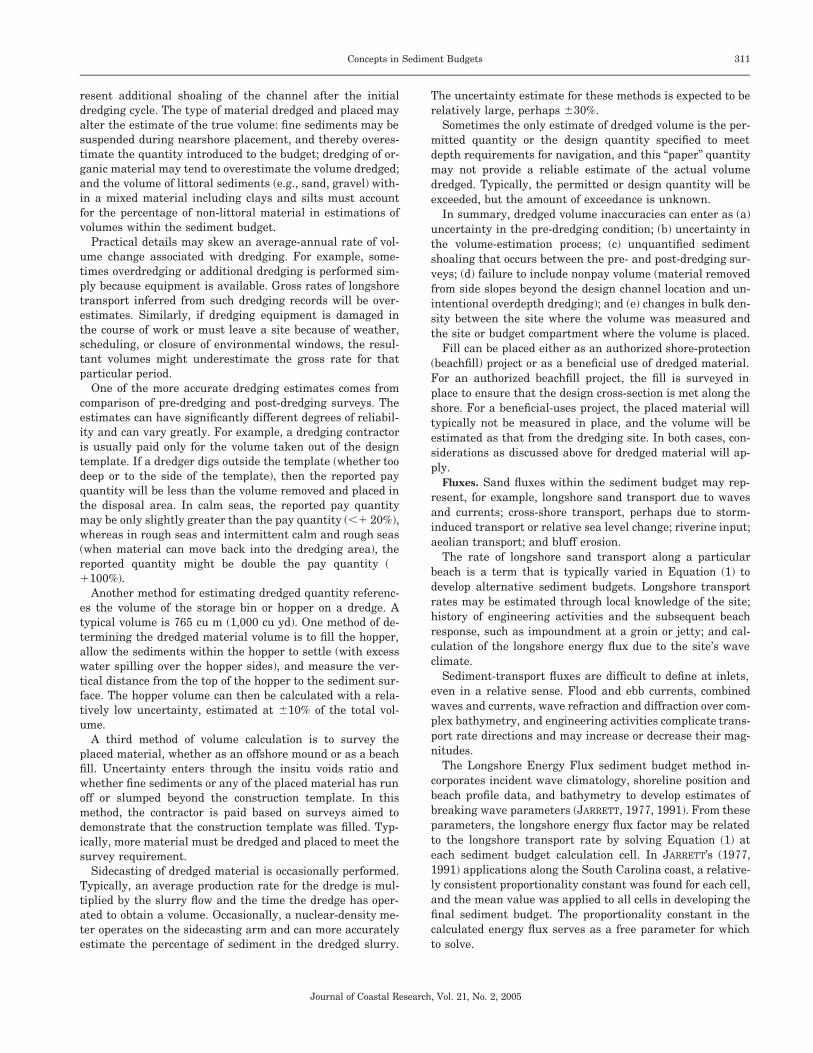
Figure 4. Example conceptual budget for Shinnecock Inlet, New York (color is specified by the user to represent either cell balance or cell erosion/ accretion).

NEW SEDIMENT BUDGET CONSIDERATIONS

The following section introduces new considerations as they apply to the formulation of sediment budgets. Some of these topics are not original to this paper, but are innovative applications of existing concepts, or represent a new empha­sis on a traditional method. Each of these approaches is dem­onstrated within the Sediment Budget Analysis System (SBAS) (KRAUS and ROSATI, 1999b; ROSATI and KRAUS 1999c, 2001), a personal computer-based program for constructing and presenting sediment budgets within a geo-referenced framework. In the next section, a short overview of SBAS1 is given.

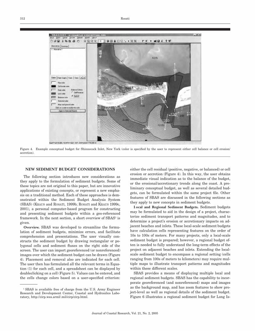
Overview. SBAS was developed to streamline the formu­lation of sediment budgets, minimize errors, and facilitate comprehension and presentations. The user visually con­structs the sediment budget by drawing rectangular or po­lygonal cells and sediment fluxes on the right side of the screen. The user can import georeferenced (or nonreferenced) images over which the sediment budget can be drawn (Figure 4). Placement and removal also are indicated for each cell. The user then has formulated all the relevant terms in Equa­tion (1) for each cell, and a spreadsheet can be displayed by doubleclicking on a cell (Figure 5). Values can be entered, and the cells change colors based on a user-specified criterion:

1 SBAS is available free of charge from the U.S. Army Engineer Research and Development Center, Coastal and Hydraulics Labo­ratory, http://cirp.wes.arml/.mil/cirp/cirp.html.

either the cell residual (positive, negative, or balanced) or cell erosion or accretion (Figure 4). In this way, the user obtains immediate visual indication as to the balance of the budget, or the erosional/accretionary trends along the coast. A pre­liminary conceptual budget, as well as several detailed bud­gets, can be formulated within the same project file. Other features of SBAS are discussed in the following sections as they apply to new concepts in sediment budgets.

Local and Regional Sediment Budgets. Sediment budgets may be formulated to aid in the design of a project, charac­terize sediment transport patterns and magnitudes, and to determine a project’s erosion or accretionary impacts on ad­jacent beaches and inlets. These local-scale sediment budgets have calculation cells representing features on the order of 10s to 100s of meters. For many projects, only a local-scale sediment budget is prepared; however, a regional budget of­ten is needed to fully understand the long-term effects of the project on adjacent beaches and inlets. Extending the local-scale sediment budget to encompass a regional setting (cells ranging from 100s of meters to kilometers) may require mul­tiple maps to illustrate transport patterns and magnitudes within these different scales.

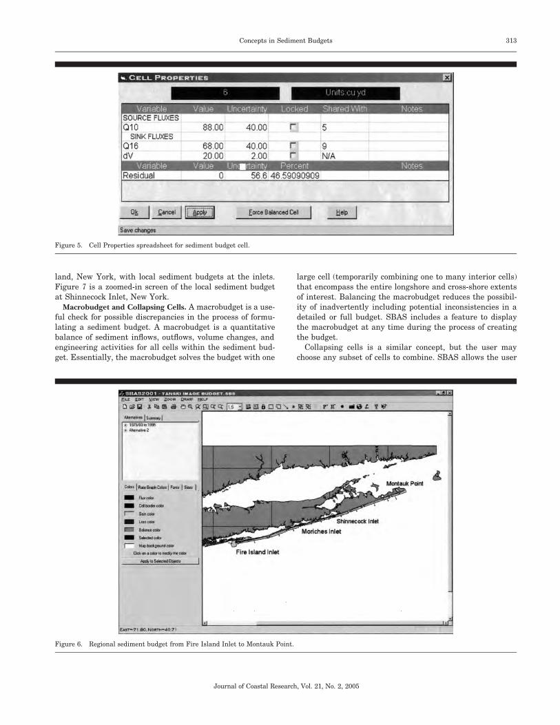
SBAS provides a means of displaying multiple local and regional sediment budgets. SBAS has the capability to incor­porate georeferenced (and nonreferenced) maps and images as the background map, and has zoom features to show pro­ject-level as well as regional details of the sediment budget. Figure 6 illustrates a regional sediment budget for Long Is-

Journal of Coastal Research, Vol. 21, No. 2, 2005

313 Concepts in Sediment Budgets

Figure 5. Cell Properties spreadsheet for sediment budget cell.

land, New York, with local sediment budgets at the inlets. Figure 7 is a zoomed-in screen of the local sediment budget at Shinnecock Inlet, New York.

Macrobudget and Collapsing Cells. A macrobudget is a use­ful check for possible discrepancies in the process of formu­lating a sediment budget. A macrobudget is a quantitative balance of sediment inflows, outflows, volume changes, and engineering activities for all cells within the sediment bud­get. Essentially, the macrobudget solves the budget with one

large cell (temporarily combining one to many interior cells) that encompass the entire longshore and cross-shore extents of interest. Balancing the macrobudget reduces the possibil­ity of inadvertently including potential inconsistencies in a detailed or full budget. SBAS includes a feature to display the macrobudget at any time during the process of creating the budget.

Collapsing cells is a similar concept, but the user may choose any subset of cells to combine. SBAS allows the user

Figure 6. Regional sediment budget from Fire Island Inlet to Montauk Point.

Journal of Coastal Research, Vol. 21, No. 2, 2005

314 Rosati

Figure 7. Local sediment budget for Shinnecock Inlet, New York.

to select cells and fluxes to combine within the area of a user-specified rectangle or polygon (Figure 8a). The selected items are then combined into one cell that is shaded to show wheth­er it is balanced (Figure 8b). The Collapsing cells feature is useful for presenting detailed local budgets within a regional budget. For presentation of the regional budget, the local budget can be collapsed into one cell by activating a rectan­gular or polygonal selection tool, thereby presenting the local budget at the same spatial scale as the regional budget. When presenting the local budget, the user can zoom-in and reinstate the combined cell to the original form.

Propagating Longshore Transport Rates. In some applica­tions, one of the more uncertain quantities in a sediment bud­get is the rate of longshore sediment transport. In creating the sediment budget, a range of feasible longshore sand transport rates is typically specified to create a series of ‘‘rep­resentative’’ budgets. However, the relationships between some of the fluxes in the budget may remain the same re­gardless of their magnitudes. For example, the transport through and over a jetty structure might be represented by 50% of the incoming transport. The capability to set these dependencies within the budget allows changes in the trans­port rate entering the sediment budget to propagate through all cells. SBAS has an option to define a linear relationship between one or more fluxes.

Uncertainty and Sensitivity Testing

Every measurement has limitations in accuracy (see KRAUS

and ROSATI, 1999a). For coastal and inlet processes, typically

direct measurement of many quantities cannot be made, such as the long-term longshore sand transport rate or the amount of material bypassing a jetty. Values of such quantities are inferred from shoreline change or bathymetric change data, obtained with predictive formulas, or through estimates based on experience and judgment, which integrate over the system. Therefore, measured or estimated values entering a sediment budget consist of a best estimate and its uncertain­ty. Uncertainty, in turn, consists of error and true uncertainty. A general source of error is limitation in the measurement process or instrument. True uncertainty is the error contrib­uted by unknowns that may not be directly related to the measurement process. Significant contributors to true uncer­tainty enter through natural variability and unknowns in the measurement process.

In coastal processes, significant contributors to true uncer­tainty enter through natural variability. Such variability in­cludes (a) temporal variability (daily, seasonal, and annual beach change), (b) spatial variability (alongshore and across shore), (c) selection of definitions (e.g., shoreline orientation, direction of random seas), and (d) unknowns such as grain size and porosity of the sediment (especially true in place­ment of dredged material). For example, a survey of the beach profile is capable of specifying the horizontal position of the mean high-water shoreline with an error less than a few centimeters with respect to a local benchmark (measure­ment error). However, a measurement made days before or after the original measurement or 50 m upcoast or downcoast may record a shoreline position differing by several meters

Journal of Coastal Research, Vol. 21, No. 2, 2005

315 Concepts in Sediment Budgets

Figure 8. Collapsing cells within SBAS. (a) Polygonal selection for collapsing cells, (b) collapsed sediment budge cells for Shinnecock Inlet.

Journal of Coastal Research, Vol. 21, No. 2, 2005

316 Rosati

from the original measurement (true uncertainty), creating ambiguity about the representative or true value. Error and uncertainty themselves are typically best estimates.

In inlet processes, uncertainty enters several ways. Two prominent ways are through limited knowledge of (a) changes in ebb- and flood-tidal delta sand volumes, and (b) the paths and relative magnitudes of transport, such as transport through and around jetties and to the tidal shoals.

Let X denote a coastal parameter to be estimated for a sed­iment budget, and suppose X is a function of several inde­pendent variables or measurements. An example is volume change for a sediment budget cell as calculated from shore­line position and profile data. Let oX denote an uncertainty in X. The uncertainty oX is considered to be an extreme plau­sible error, and it carries a sign, that is,

oX = ±loXl (4)

If X is a function of the independent variables x, y, and z, by assuming the uncertainty in each variable is reasonably small, a Taylor series gives to lowest order,

aX aX aXX + oX = X + ox + oy + oz (5)rms rms aX ay az

so that the maximum uncertainty in X is

aX aX aX oX = ox + oy + oz (6)max ax ay az

to lowest order. Because the ox, oy, oz, etc., each contain a sign (±), the partial derivatives in Equations 5 and 6 are interpreted as absolute (positive) values. That is, in uncer­tainty analysis we form extreme values by consistently ap­plying (±) to each term to avoid cancellation between and among terms.

From Equations 5 and 6, and other assumptions (see TAY­

LOR, 1997), general relationships can be derived. If the vari­able X is a sum or difference of several independent param­eters as X = x + y - z + . . . - . . . , then the root-mean­square (rms) uncertainty is

2 2 2oXrms = Y(ox) + (oy) + (oz) + · · · (7)

The validity of this expression rests on the assumptions that the individual uncertainties are independent and random. The rms error accounts for the uncertainty in uncertainty by giving a value that is not an extreme, such as oXmax.

If the variable X is expressed as another variable raised to a power, X = axn, where a is a constant and has no uncer­tainty, then, from Equation 6,

oX ox = ln l (8)

lX l x ll

Equation 8 conveniently expresses error as a fractional un­certainty or percentage ratio of uncertainty.

Suppose the quantity entering the budget is expressed as a product or quotient of independent variables as X = xyz or as xy/z. In either case, the uncertainty in X is

2 2 2oX ox oy oz

= + + (9) Xrms

x y z

The errors are additive whether a variable enters as a prod-

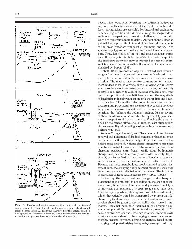
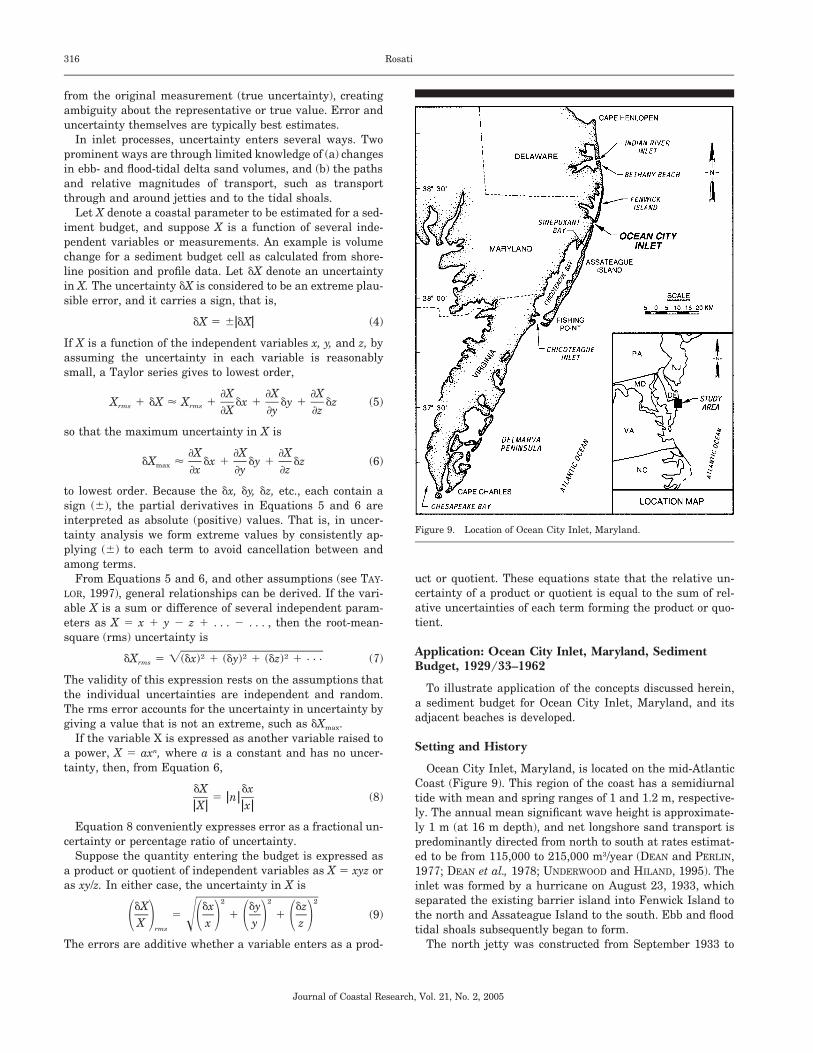
Figure 9. Location of Ocean City Inlet, Maryland.

uct or quotient. These equations state that the relative un­certainty of a product or quotient is equal to the sum of rel­ative uncertainties of each term forming the product or quo­tient.

Application: Ocean City Inlet, Maryland, Sediment Budget, 1929/33–1962

To illustrate application of the concepts discussed herein, a sediment budget for Ocean City Inlet, Maryland, and its adjacent beaches is developed.

Setting and History

Ocean City Inlet, Maryland, is located on the mid-Atlantic Coast (Figure 9). This region of the coast has a semidiurnal tide with mean and spring ranges of 1 and 1.2 m, respective­ly. The annual mean significant wave height is approximate­ly 1 m (at 16 m depth), and net longshore sand transport is predominantly directed from north to south at rates estimat­ed to be from 115,000 to 215,000 m3/year (DEAN and PERLIN, 1977; DEAN et al., 1978; UNDERWOOD and HILAND, 1995). The inlet was formed by a hurricane on August 23, 1933, which separated the existing barrier island into Fenwick Island to the north and Assateague Island to the south. Ebb and flood tidal shoals subsequently began to form.

The north jetty was constructed from September 1933 to

Journal of Coastal Research, Vol. 21, No. 2, 2005

Concepts in Sediment Budgets 317

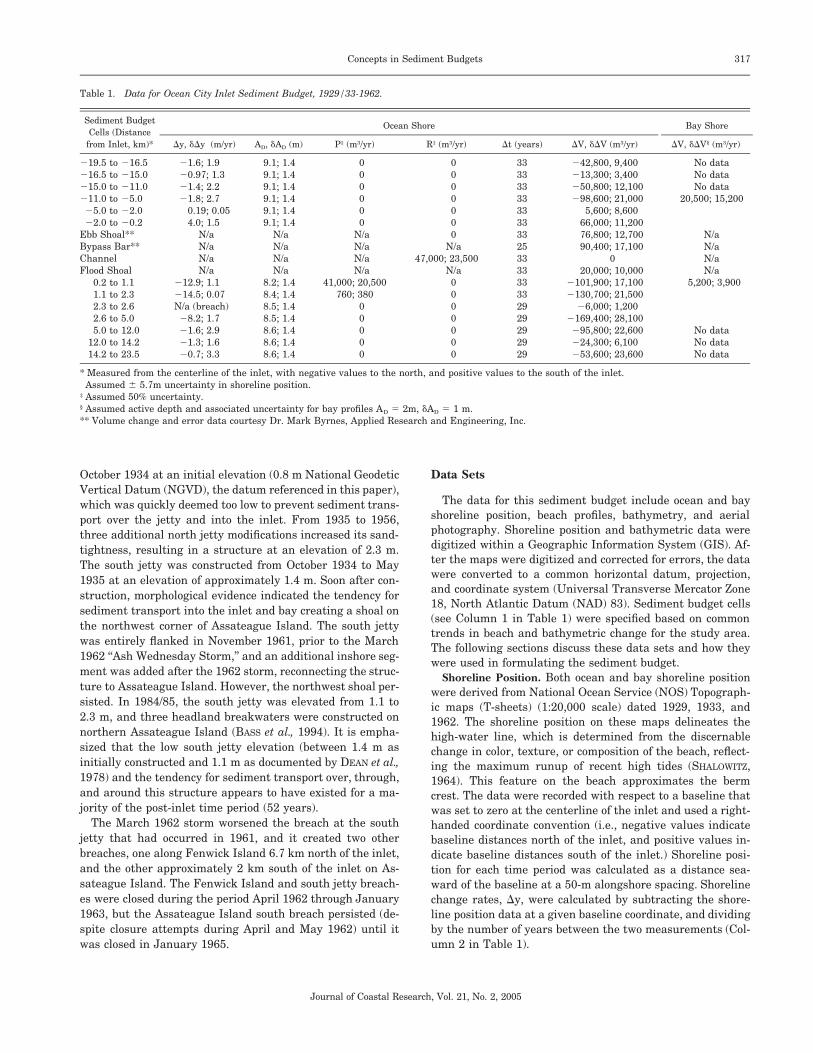
Table 1. Data for Ocean City Inlet Sediment Budget, 1929/33-1962.

Sediment Budget Cells (Distance

from Inlet, km)* Ly, oLy† (m/yr) AD, oAD (m) P‡ (m3/yr)

Ocean Shore

R‡ (m3/yr) Lt (years) LV, oLV (m3/yr)

Bay Shore

LV, oLV§ (m3/yr)

-19.5 to -16.5 -16.5 to -15.0 -15.0 to -11.0 -11.0 to -5.0 -5.0 to -2.0 -2.0 to -0.2

Ebb Shoal** Bypass Bar** Channel Flood Shoal

0.2 to 1.1 1.1 to 2.3 2.3 to 2.6 2.6 to 5.0 5.0 to 12.0

12.0 to 14.2 14.2 to 23.5

-1.6; 1.9 -0.97; 1.3 -1.4; 2.2 -1.8; 2.7

0.19; 0.05 4.0; 1.5

N/a N/a N/a N/a

-12.9; 1.1 -14.5; 0.07 N/a (breach) -8.2; 1.7 -1.6; 2.9 -1.3; 1.6 -0.7; 3.3

9.1; 1.4 9.1; 1.4 9.1; 1.4 9.1; 1.4 9.1; 1.4 9.1; 1.4

N/a N/a N/a N/a

8.2; 1.4 8.4; 1.4 8.5; 1.4 8.5; 1.4 8.6; 1.4 8.6; 1.4 8.6; 1.4

0 0 0 0 0 0

N/a N/a N/a N/a

41,000; 20,500 760; 380

0 0 0 0 0

0 0 0 0 0 0 0

N/a 47,000; 23,500

N/a 0 0 0 0 0 0 0

33 33 33 33 33 33 33 25 33 33 33 33 29 29 29 29 29

-42,800, 9,400 -13,300; 3,400 -50,800; 12,100 -98,600; 21,000

5,600; 8,600 66,000; 11,200 76,800; 12,700 90,400; 17,100

0 20,000; 10,000

-101,900; 17,100 -130,700; 21,500

-6,000; 1,200 -169,400; 28,100 -95,800; 22,600 -24,300; 6,100 -53,600; 23,600

No data No data No data

20,500; 15,200

N/a N/a N/a N/a

5,200; 3,900

No data No data No data

* Measured from the centerline of the inlet, with negative values to the north, and positive values to the south of the inlet. † Assumed ± 5.7m uncertainty in shoreline position. ‡ Assumed 50% uncertainty. § Assumed active depth and associated uncertainty for bay profiles AD = 2m, oAD = 1 m. ** Volume change and error data courtesy Dr. Mark Byrnes, Applied Research and Engineering, Inc.

October 1934 at an initial elevation (0.8 m National Geodetic Vertical Datum (NGVD), the datum referenced in this paper), which was quickly deemed too low to prevent sediment trans­port over the jetty and into the inlet. From 1935 to 1956, three additional north jetty modifications increased its sand-tightness, resulting in a structure at an elevation of 2.3 m. The south jetty was constructed from October 1934 to May 1935 at an elevation of approximately 1.4 m. Soon after con­struction, morphological evidence indicated the tendency for sediment transport into the inlet and bay creating a shoal on the northwest corner of Assateague Island. The south jetty was entirely flanked in November 1961, prior to the March 1962 ‘‘Ash Wednesday Storm,’’ and an additional inshore seg­ment was added after the 1962 storm, reconnecting the struc­ture to Assateague Island. However, the northwest shoal per­sisted. In 1984/85, the south jetty was elevated from 1.1 to 2.3 m, and three headland breakwaters were constructed on northern Assateague Island (BASS et al., 1994). It is empha­sized that the low south jetty elevation (between 1.4 m as initially constructed and 1.1 m as documented by DEAN et al., 1978) and the tendency for sediment transport over, through, and around this structure appears to have existed for a ma­jority of the post-inlet time period (52 years).

The March 1962 storm worsened the breach at the south jetty that had occurred in 1961, and it created two other breaches, one along Fenwick Island 6.7 km north of the inlet, and the other approximately 2 km south of the inlet on As­sateague Island. The Fenwick Island and south jetty breach­es were closed during the period April 1962 through January 1963, but the Assateague Island south breach persisted (de­spite closure attempts during April and May 1962) until it was closed in January 1965.

Data Sets

The data for this sediment budget include ocean and bay shoreline position, beach profiles, bathymetry, and aerial photography. Shoreline position and bathymetric data were digitized within a Geographic Information System (GIS). Af­ter the maps were digitized and corrected for errors, the data were converted to a common horizontal datum, projection, and coordinate system (Universal Transverse Mercator Zone 18, North Atlantic Datum (NAD) 83). Sediment budget cells (see Column 1 in Table 1) were specified based on common trends in beach and bathymetric change for the study area. The following sections discuss these data sets and how they were used in formulating the sediment budget.

Shoreline Position. Both ocean and bay shoreline position were derived from National Ocean Service (NOS) Topograph­ic maps (T-sheets) (1:20,000 scale) dated 1929, 1933, and 1962. The shoreline position on these maps delineates the high-water line, which is determined from the discernable change in color, texture, or composition of the beach, reflect­ing the maximum runup of recent high tides (SHALOWITZ, 1964). This feature on the beach approximates the berm crest. The data were recorded with respect to a baseline that was set to zero at the centerline of the inlet and used a right-handed coordinate convention (i.e., negative values indicate baseline distances north of the inlet, and positive values in­dicate baseline distances south of the inlet.) Shoreline posi­tion for each time period was calculated as a distance sea­ward of the baseline at a 50-m alongshore spacing. Shoreline change rates, Ly, were calculated by subtracting the shore­line position data at a given baseline coordinate, and dividing by the number of years between the two measurements (Col­umn 2 in Table 1).

Journal of Coastal Research, Vol. 21, No. 2, 2005

318 Rosati

After 1920, NOS T-sheets were compiled from rectified ae­rial photography, a procedure which has a potential error of ± 5 m due to the interpretation of the remotely-obtained shoreline position. There are also errors in digitizing the shoreline from the T-sheets associated with equipment and operation accuracy and precision. Digitizing tables used in this study have an absolute accuracy of 0.1 mm, which trans­lates to ± 2 m for a 1:20,000 scale map. In addition, errors associated with the digitizing process itself were is estimated to be ± 2 m, for a total root-mean-square (rms) uncertainty associated with the shoreline position data, oLy = Y52 + 22 + 22 = 5.7 m. If we assume that errors associated with the digitizing process are random, i.e., they tend to can­cel for a large number of data points, then this value of un­certainty represents an upper limit.

Beach Profiles. Beach profiles for Fenwick and Assateague Islands dated June 1976 (earliest data set available) were used to define the active depth of the ocean beach, AD. These profiles were taken by a field crew using a rod and level. Erosion of the beaches, including overwash of the barriers was significant during the 1962 Ash Wednesday storm, es­pecially on Assateague Island. However, in the absence of other data, it was assumed that the 1976 profile data were representative of the period 1933 to 1962.

Active depth represents the part of the beach profile that is eroding or accreting during the time period of consider­ation, and is typically defined as the absolute sum of the berm crest elevation, B, and depth of closure, Dc,

AD = B + Dc (11)

Berm crest, depth of closure, and average active depth values were calculated (oceanside) or estimated (bayside) for each sediment budget cell.

The uncertainties associated with determination of, B, and, Dc, include errors due to the measurement method and errors in interpreting the values. KRAUS and HEILMAN (1988) mea­sured the accuracy in elevation measurements for distances from the survey station ranging from 10 m to 1 km. They determined that potential error in elevation measurements was between 2 and 8 mm for measurements located from 10 m to 1 km from the survey station. The Ocean City profile data analyzed herein transverse less than 1 km, and thus these error estimates are adopted for the present study. For ocean profiles, B (ocean) ranged from 2.1 to 3.0 m, with an associated variation for a given sediment budget cell ranging from 0.4 to 0.6 m. Thus, the rms uncertainty associated with the ocean berm crest elevation is estimated to be oB(ocean) = Y0.0082 + 0.42 to 0.62 = 0.4 to 0.6 m. Uncertainty in hor­izontal position is assumed to be negligible.

Profile data for the bay shoreline were not available. Based on interviews with people familiar with the site, and those who have conducted previous field measurements at Ocean City Inlet, it was estimated that a reasonable estimate for

←

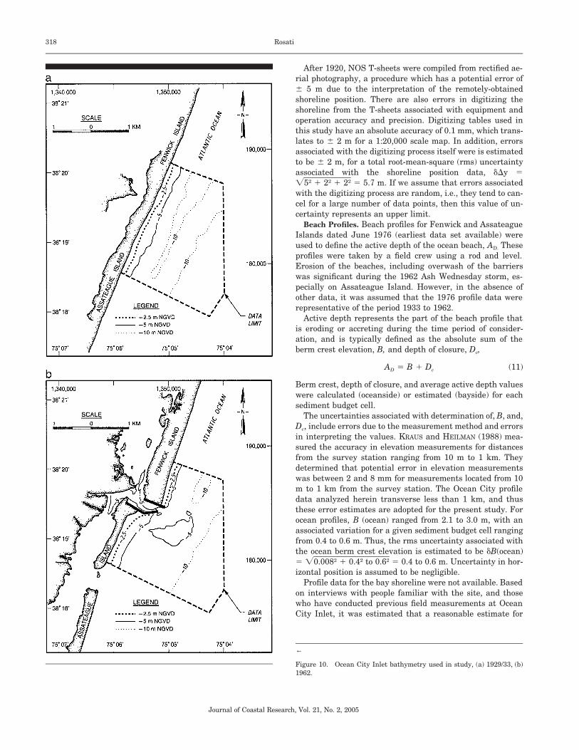
Figure 10. Ocean City Inlet bathymetry used in study, (a) 1929/33, (b) 1962.

Journal of Coastal Research, Vol. 21, No. 2, 2005

319 Concepts in Sediment Budgets

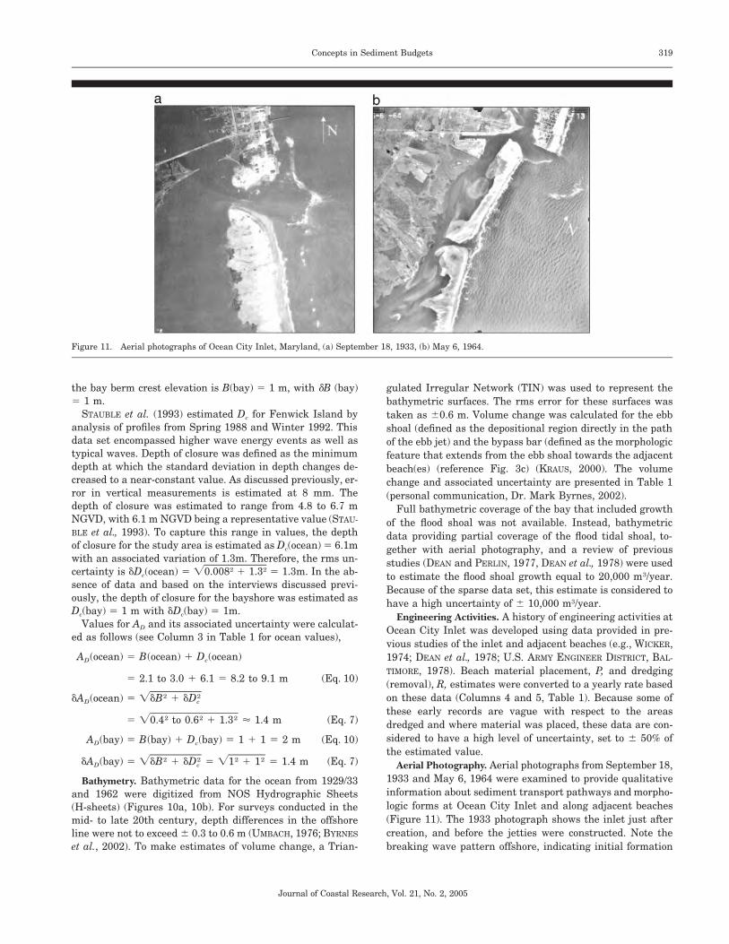
Figure 11. Aerial photographs of Ocean City Inlet, Maryland, (a) September 18, 1933, (b) May 6, 1964.

the bay berm crest elevation is B(bay) = 1 m, with oB (bay) = 1 m.

STAUBLE et al. (1993) estimated Dc for Fenwick Island by analysis of profiles from Spring 1988 and Winter 1992. This data set encompassed higher wave energy events as well as typical waves. Depth of closure was defined as the minimum depth at which the standard deviation in depth changes de­creased to a near-constant value. As discussed previously, er­ror in vertical measurements is estimated at 8 mm. The depth of closure was estimated to range from 4.8 to 6.7 m NGVD, with 6.1 m NGVD being a representative value (STAU­

BLE et al., 1993). To capture this range in values, the depth of closure for the study area is estimated as Dc(ocean) = 6.1m with an associated variation of 1.3m. Therefore, the rms un­certainty is oDc(ocean) = Y0.0082 + 1.32 = 1.3m. In the ab­sence of data and based on the interviews discussed previ­ously, the depth of closure for the bayshore was estimated as Dc(bay) = 1 m with oDc(bay) = 1m.

Values for AD and its associated uncertainty were calculat­ed as follows (see Column 3 in Table 1 for ocean values),

AD(ocean) = B(ocean) + Dc(ocean)

= 2.1 to 3.0 + 6.1 = 8.2 to 9.1 m (Eq. 10)

oAD(ocean) = YoB2 + oDc 2

2 2 2= Y0.4 to 0.6 + 1.3 = 1.4 m (Eq. 7)

AD(bay) = B(bay) + Dc(bay) = 1 + 1 = 2 m (Eq. 10)

2 2 2 2oAD(bay) = YoB + oDc = Y1 + 1 = 1.4 m (Eq. 7)

Bathymetry. Bathymetric data for the ocean from 1929/33 and 1962 were digitized from NOS Hydrographic Sheets (H-sheets) (Figures 10a, 10b). For surveys conducted in the mid- to late 20th century, depth differences in the offshore line were not to exceed ± 0.3 to 0.6 m (UMBACH, 1976; BYRNES

et al., 2002). To make estimates of volume change, a Trian­

gulated Irregular Network (TIN) was used to represent the bathymetric surfaces. The rms error for these surfaces was taken as ±0.6 m. Volume change was calculated for the ebb shoal (defined as the depositional region directly in the path of the ebb jet) and the bypass bar (defined as the morphologic feature that extends from the ebb shoal towards the adjacent beach(es) (reference Fig. 3c) (KRAUS, 2000). The volume change and associated uncertainty are presented in Table 1 (personal communication, Dr. Mark Byrnes, 2002).

Full bathymetric coverage of the bay that included growth of the flood shoal was not available. Instead, bathymetric data providing partial coverage of the flood tidal shoal, to­gether with aerial photography, and a review of previous studies (DEAN and PERLIN, 1977, DEAN et al., 1978) were used to estimate the flood shoal growth equal to 20,000 m3/year. Because of the sparse data set, this estimate is considered to have a high uncertainty of ± 10,000 m3/year.

Engineering Activities. A history of engineering activities at Ocean City Inlet was developed using data provided in pre­vious studies of the inlet and adjacent beaches (e.g., WICKER, 1974; DEAN et al., 1978; U.S. ARMY ENGINEER DISTRICT, BAL­

TIMORE, 1978). Beach material placement, P, and dredging (removal), R, estimates were converted to a yearly rate based on these data (Columns 4 and 5, Table 1). Because some of these early records are vague with respect to the areas dredged and where material was placed, these data are con­sidered to have a high level of uncertainty, set to ± 50% of the estimated value.

Aerial Photography. Aerial photographs from September 18, 1933 and May 6, 1964 were examined to provide qualitative information about sediment transport pathways and morpho­logic forms at Ocean City Inlet and along adjacent beaches (Figure 11). The 1933 photograph shows the inlet just after creation, and before the jetties were constructed. Note the breaking wave pattern offshore, indicating initial formation

Journal of Coastal Research, Vol. 21, No. 2, 2005

320 Rosati

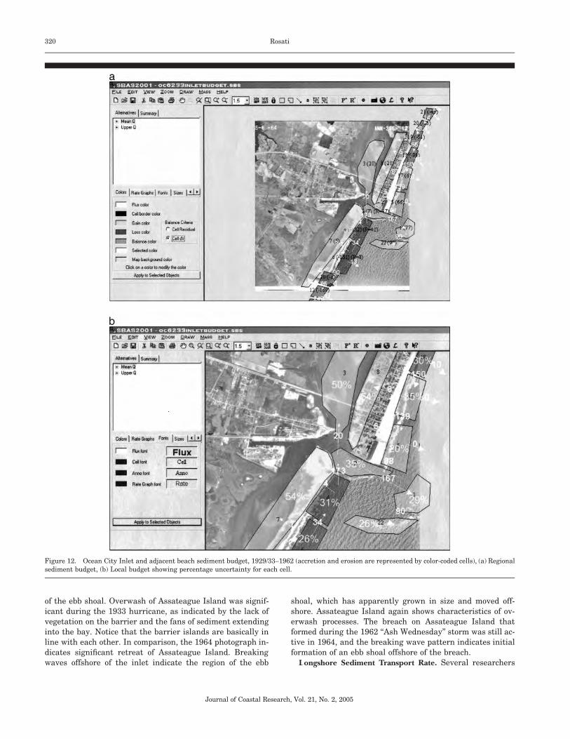
Figure 12. Ocean City Inlet and adjacent beach sediment budget, 1929/33–1962 (accretion and erosion are represented by color-coded cells), (a) Regional sediment budget, (b) Local budget showing percentage uncertainty for each cell.

of the ebb shoal. Overwash of Assateague Island was signif­icant during the 1933 hurricane, as indicated by the lack of vegetation on the barrier and the fans of sediment extending into the bay. Notice that the barrier islands are basically in line with each other. In comparison, the 1964 photograph in­dicates significant retreat of Assateague Island. Breaking waves offshore of the inlet indicate the region of the ebb

shoal, which has apparently grown in size and moved off­shore. Assateague Island again shows characteristics of ov­erwash processes. The breach on Assateague Island that formed during the 1962 ‘‘Ash Wednesday’’ storm was still ac­tive in 1964, and the breaking wave pattern indicates initial formation of an ebb shoal offshore of the breach.

Longshore Sediment Transport Rate. Several researchers

Journal of Coastal Research, Vol. 21, No. 2, 2005

321 Concepts in Sediment Budgets

have estimated values of longshore sediment transport for Ocean City. DEAN and PERLIN (1977) estimated that the north jetty was fully impounded by 1972, with an impoundment rate ranging from 115,000 to 153,000 cu m/year. There is also a generally-accepted nodal area in the net longshore sedi­ment transport at the Maryland-Delaware state line. The lo­cation of this nodal area can vary annually. DOUGLASS (1985) estimated an average net longshore sediment transport rate equal to 214,000 cu m/year based on hindcast data from 1956–1975. Based on this work and the growth of the ebb and flood shoals, UNDERWOOD and HILAND (1995) adopted a southerly-directed net transport equal to 212,800 cu m/year. In an application of a morphologic change model, KRAUS

(2000) specified 150,000 cu m/year as an upper limit to the net longshore sediment transport rate.

For the sediment budget herein, an average net longshore sediment transport rate north of the inlet, outside the im­poundment zone of the north jetty, was taken as 150,000 cu m/yr with an uncertainty of ± 50,000 cu m/year.

Transport rates to the offshore were estimated to be 10% of the volume change within the cell, with an uncertainty of 10%.

Calculations

The shoreline position data were used to calculate volume change, LV (m3/year), for each ocean and bay shoreline cell,

LV = LyADLx (11)

where Ly is the average shoreline change rate for the sedi­ment budget cell (m/year), AD is the average active depth for the cell (m), and Lx represents the length of the sediment budget cell (m).

These data were entered into SBAS, and a regional sedi­ment budget was developed as shown in Figure 12. Cells may be color coded to indicate net accretion or erosion of the cell. The net volume change from 1933 to 1962 resulted in accre­tion areas in the vicinity of the inlet channels and shoals, on the updrift beach, and overwash of the barrier islands into the bay. The remaining adjacent beaches lost sediment through longshore transport and overwash processes.

SBAS allows the user to record uncertainty for each value entered in the sediment budget. Then, for each cell, collapsed cell, and the entire budget, SBAS calculates the root-mean­square (rms) uncertainty. The user can apply the rms uncer­tainty to indicate the relative confidence that can be given to each cell in the sediment budget, and in comparing alterna­tives that represent different assumptions about the sedi­ment budget. Figure 12b shows the percentage uncertainty for each cell. The percentage of uncertainty is calculated as the total magnitude of uncertainty for that cell divided by the absolute value summation of the fluxes, volume change, placement, and removal for that cell. Uncertainty for the bay cells and flood shoal is greater than uncertainty in the vicin­ity of the inlet and adjacent beaches, indicating the level of confidence we can use when interpreting the budget. A sed­iment budget formulated with a more extensive bay data set would have a lower value of uncertainty. Integrating uncer­tainty into the sediment budget allows engineers, managers,

local government officials, and community members to read­ily grasp an understanding of the reliability of values within the budget.

CONCLUSIONS

Sediment budgets are a time-tested means of understand­ing the sediment patterns and magnitudes for riverine and coastal areas. With knowledge gained through numerous ap­plications and the advent of visually-based computer inter­faces, several new concepts have emerged that streamline the formulation process and improve the reliability of sediment budgets. These concepts were demonstrated for regional sed­iment budgets at Long Island, New York, and Ocean City Inlet, Maryland within the Sediment Budget Analysis Sys­tem (SBAS). Considering the regional budget and developing values of root-mean-square uncertainty are an essential com­ponent of modern sediment budgets. Calculation of the un­certainty together with the sediment budget itself allows the reliability of this methodology to be estimated, and to im­prove its value as a framework for coastal and riverine plan­ning and project design.

ACKNOWLEDGMENTS

This paper was prepared as an activity of the Inlet Chan­nels and Adjacent Shorelines Work Unit of the Coastal Inlets Research Program conducted at the Coastal and Hydraulics Laboratory. Dr. Nicholas C. Kraus and Dr. Mark R. Byrnes are thanked for stimulating discussions and review of the manuscript. Collaboration with the New York and Baltimore Districts is much appreciated in preparation of the respective sediment budgets. Thanks to Dr. Terry Healy for helpful re­view comments. Permission was granted by Headquarters, U.S. Army Corps of Engineers, to publish this information.

NOTATION

The following symbols are used in this paper:

a = constant with no uncertainty AD = active depth for sediment budget cell B = berm crest elevation for sediment budget cell

Dc = depth of closure for sediment budget cell n = exponential constant P = placement of sediment within sediment budget

cell Qgross = gross longshore sediment transport rate

QL = longshore sediment transport rate to the left (seaward-facing observer)

Qnet = net longshore sediment transport rate QR = longshore sediment transport rate to the right

(seaward-facing observer) Qsink = sediment flux exiting a sediment budget cell

Qsource = sediment flux entering a sediment budget cell R = removal of sediment from sediment budget cell

Residual = balance for sediment budget cell t = time

X = engineering quantity to be estimated x = independent variable y = independent variable

Journal of Coastal Research, Vol. 21, No. 2, 2005

322 Rosati

z = independent variable oAD = uncertainty in active depth oB = uncertainty in berm crest elevation

oDc = uncertainty in depth of closure LV = volume change rate for sediment budget cell Lt = time period of calculation ox = uncertainty in independent variable x oX = uncertainty in engineering quantity X Lx = length of sediment budget cell

oLx = uncertainty in length of sediment budget cell oy = uncertainty in independent variable y Ly = average shoreline change rate for sediment bud­

get cell oLy = uncertainty in average shoreline change rate for

sediment budget cell oz = uncertainty in independent variable z

Subscript max = maximum rms = root-mean-square

LITERATURE CITED

BASS, G.P.; FULFORD, E.T.; UNDERWOOD, S.G., and PARSON, L.E., 1994. Rehabilitation of the South Jetty, Ocean City, Maryland. Technical Report CERC-94-6, Coastal Engineering Research Cen­ter, Vicksburg, MS, 60p.

BLACK, K. and HEALY, T.R. 1983. Side-scan Sonar Survey, Northland Forestry Port Investigation. Northland Harbour Board, 88p.

BODGE, K.R., 1993. Gross Transport Effects at Inlets. Proceedings of the 6th Annual National Conference on Beach Preservation Tech­nology (Tallahassee, FL, Florida Shore & Beach Preservation As­sociation), pp. 112–127.

BODGE, K.R., 1999. Inlet Impacts and Families of Solutions for Inlet Sediment Budgets. Proceedings, Coastal Sediments ’99, (Reston, VA, ASCE,) pp. 703–718.

BOWEN, A.J. and INMAN, D.L., 1966. Budget of Littoral Sand in the Vicinity of Point Arguello, California. U.S. Army Coastal Engi­neering Research Center, Technical Memorandum No. 19, 56p.

BYRNES, M.R.; LI, F., and BAKER, J.L., 2002. Quantifying Potential Measurement Errors Associated with Bathymetric Change Anal­ysis. Coastal Engineering Technical Note IV-50, U.S. Army Engi­neer Research and Development Center, Coastal and Hydraulics Laboratory, Vicksburg, MS, 17p.

CALDWELL, J.M., 1966. Coastal Processes and Beach Erosion. Journal of the Society of Civil Engineers, 53 (2), 142–157.

CARR, E.E. and KRAUS, N.C., 2001. Morphologic Asymmetries at En­trances to Tidal Inlets. Coastal Engineering Technical Note IV-33, U.S. Army Engineer Waterways Experiment Station, Coastal and Hydraulics Laboratory, Vicksburg, MS, 16p.

DEAN, R.G. and PERLIN, M., 1977. Coastal Engineering Study of Ocean City Inlet, Maryland. Proceedings, Coastal Sediments ’77 (Reston, VA, ASCE), pp. 520–540.

DEAN, R. G.; PERLIN, M., and DALLY, W., 1978. A Coastal Engineering Study of Shoaling in Ocean City Inlet. Prepared for U.S. Army Engineer District, Baltimore, under contract with the University of Delaware, Newark, DE, 135p.

DOLAN, T.J.; CASTENS, P.G.; SONU, C.J., and EGENSE, A.K., 1987. Re­view of Sediment Budget Methodology: Oceanside Littoral Cell, Cal­ifornia. Proceedings, Coastal Sediments ’87 (Reston, VA, ASCE), pp. 1289–1304.

INMAN, D.L. and FRAUTSCHY, J.D., 1966. Littoral Processes and the Development of Shorelines. Proceedings Coastal Engineering Spe­cialty Conference (Reston, VA, ASCE), pp. 511–536.

JARRETT, J.T., 1977. Sediment Budget Analysis Wrightsville Beach

to Kure Beach, N.C. Proceedings Coastal Sediments 77 (Reston, VA, ASCE), pp. 986–1005.

JARRETT, J.T., 1991. Coastal Sediment Budget Analysis Techniques. Proceedings Coastal Sediments ’91 (Reston, VA, ASCE), pp. 2223– 2233.

KANA, T. and STEVENS, F., 1992. Coastal Geomorphology and Sand Budgets Applied to Beach Nourishment. Proceedings Coastal En­gineering Practice ’92 (Reston, VA, ASCE), pp. 29–44.

KOMAR, P.D., 1996. The Budget of Littoral Sediments, Concepts and Applications. Shore and Beach, 64(3), 18–26.

KOMAR, P.D., 1998. Beach Processes and Sedimentation. Prentice-Hall, Inc., Simon & Schuster, Upper Saddle River, NJ, pp. 66–72.

KRAUS, N.C., 2000. Reservoir Model of Ebb-Tidal Shoal Evolution and Sand Bypassing. Journal of Waterway, Port, Coastal, and Ocean Engineering, 126(6), 305–313.

KRAUS, N.C. and HEILMAN, D.J., 1998. Comparison of Beach Profiles at a Seawall and Groins, Corpus Christi, Texas. Shore and Beach, 63(2), pp. 4–13.

KRAUS, N.C. and ROSATI, J.D., 1999a. Estimation of Uncertainty in Coastal-Sediment Budgets at Inlets. Coastal Engineering Techni­cal Note CETN IV-16, U.S. Army Engineer Research and Devel­opment Center, Coastal and Hydraulics Laboratory, Vicksburg, MS, 12p.

KRAUS, N.C. and ROSATI, J.D., 1999b. Estimating Uncertainty in Coastal Inlet Sediment Budgets. Proceedings, 12th Annual Nation­al Conference on Beach Preservation Technology (Tallahassee, FL, Florida Shore & Beach Preservation Association), pp. 287–302.

ROSATI, J. D. and KRAUS, N.C., 1999c. Formulation of Sediment Bud­gets at Inlets. Coastal Engineering Technical Note CETN-IV-15, U.S. Army Engineer Research and Development Center, Coastal and Hydraulics Laboratory, Vicksburg, MS, 20p.

ROSATI, J.D. and KRAUS, N.C., 2001. Sediment Budget Analysis Sys­tem: Upgrade for Regional Applications. Coastal and Hydraulics Engineering Technical Note CHETN-XIV-3, U.S. Engineer Re­search and Development Center, Vicksburg, MS, 13p.

SHALOWITZ, A.L., 1964. Shore and Sea Boundaries. Volume Two: In­terpretation and Use of Coast and Geodetic Survey Data, Publi­cation 10-1, US Department of Commerce, Coast and Geodetic Survey, 749p.

STAUBLE, D.K.; GARCIA, A.W.; KRAUS, N.C.; GROSSKOPF, W.G., and BASS, G.P., 1993. Beach Nourishment Project Response and Design Evaluation: Ocean City, Maryland. Report 1, 1988–1992. Technical Report CERC-93-13, USAE Waterways Experiment Station, Vicksburg, MS, 372p.

TAYLOR, J. R., 1997. An introduction to error analysis. 2nd ed., Uni­versity Science Books, Sausolito, CA, 327p.

UMBACH, M.J., 1976. Hydrographic Manual—Fourth Edition. U.S. Department of Commerce, Rockville, MD, 400p.

UNDERWOOD, S.G. and HILAND, M.W., 1995. Historical development of Ocean City Inlet Ebb Shoal and its effect on Northern Assateague Island. Report prepared for the U.S. Army Engineer Waterways Experiment Station, Coastal Engineering Research Center, Vicks­burg, MS, 130p.

U.S. ARMY CORPS OF ENGINEERS, 1957. Shore of New Jersey from Sandy Hook to Barnegat Inlet, Beach Erosion Control Study. Letter from the Secretary of the Army, House Document No. 361, 84th Congress, 2nd Session, U.S. Government Printing Office, Wash­ington, DC.

U.S. ARMY CORPS OF ENGINEERS, 1958. Shore of New Jersey from Sandy Hook to Barnegat Inlet, Beach Erosion Control Study. Letter from the Secretary of the Army, House Document No. 362, 85th Congress, 2nd Session, U.S. Government Printing Office, Wash­ington, DC.

U.S. ARMY ENGINEER DISTRICT, BALTIMORE, 1978. Ocean City, Mary­land—Reconnaissance Report for Major Rehabilitation Program. Baltimore, MD.

WICKER, C.F., 1974. Report on Shoaling, Ocean City Inlet Maryland to Commercial Fish Harbor. Unpublished document, U.S. Army Engineer District, Baltimore, Baltimore, MD.

Journal of Coastal Research, Vol. 21, No. 2, 2005