Embed Size (px)
DESCRIPTION
Concepts and Methods for Assessing and Evaluating Water System Response to Climate Change. Capacity Building Programme on the Economics of Climate Change Adaptation (ECCA) Supporting National/Sub-national Adaptation Planning and Action Siem Reap, Cambodia 17-20 Sept. 2014. - PowerPoint PPT Presentation
Citation preview

Concepts and Methods for Assessing and Evaluating Water System Response to Climate Change
Capacity Building Programme on the Economics of Climate Change Adaptation (ECCA)
Supporting National/Sub-national Adaptation Planning and Action
Siem Reap, Cambodia17-20 Sept. 2014
Brian H. HurdProfessor of Agricultural Economics & Agricultural BusinessNew Mexico State University bhurd @ nmsu.edu http://agecon.nmsu.edu/bhurd

Overview• Overview of adaptation concepts• Current water issues and problems
along America’s Rio Grande • Conjunctive-use externalities• Basic concepts and strategies in Hydro-
Economic Modeling• Case Study: Rio Grande
Break
• Systems modeling basic structure, concepts and application • Case Study: Systems modeling of small community irrigation systems in New Mexico• Ideas and strategies for modeling adaptation in watershed assessments

Changing Hydrographs
• Water storage and distribution systems?
• Urban and rural water users?
• Water quality?• Hydropower?• Recreational and cultural
functions?• Riparian ecosystems and
migratory patterns?
What does it mean for?
Model assumptions
temperature ↑ 4°C
Precipitation ↑ 10%

Droughts and FloodsRio Grande Drought: Elephant Butte Reservoir
(1) 89% June 2, 1994
• (2) 3% July 8, 2013
Sept 2014, Pakistan

Climate Adaptation Related Terms and Concepts • Climatic Vulnerability - Measures a system’s susceptibility to climate change as a function of exposure to climate,
sensitivity to climatic changes, and adaptive capacity
• Adaptive Capacity - The ability of systems, organizations, and individuals to:
– Adjust to realized and potential changes and disturbance events
– Take advantage of existing and emerging opportunities
– Successfully cope with adverse consequences, mitigate damages, and/or recover
from system failures
• Adaptation - A deliberate change in system design, function or behavior in
response to or anticipation of external events or changing conditions.
– Reactive (autonomous) adaptation – disturbance occurs and systems absorb impacts
and attempt restoration to pre-disturbed conditions
– Proactive (anticipatory) adaptation – nature and timing of disturbance is anticipated and
systems are appropriately reorganized to improve their capacity to avert adverse damages
and to leverage resulting opportunities
• Adaptation is successful if, following a change or disturbance, the level of services and functionality (i.e., social value) is
approximately maintained or restored.

Timing Adaptations: the Relative Cost and Success of Reactive versus Proactive Adaptation
• Benefits of delayed action – Increased accuracy based on evolving
knowledge and information– Postponed expenditures and possibly
better technologies and lower unit costs
• Risks of delayed action– Less successful adaptation
• More welfare losses and service disruptions
• Greater likelihood of irreversible losses
– Reduced adjustment time
Time
Net Social Value
+
-
Reactive
Proactive

Elephant Butte Irrigation District (EBID)
El Paso County WaterImprovement District #1
(EP No. 1)
Rio Grande Compact (Colorado, New Mexico, Texas, 1939)
1906 Treaty with Mexico (for “Equitable Distribution of the Waters of
the Rio Grande” delivers 60 (kaf/yr) to Ciudad Juárez)
Rio Grande Project (U.S. Bureau of Reclamation project;
initiated 1905; Elephant Butte Dam, 1916; Caballo Dam, 1938)
Water in the Southwest United States: Rio Grande
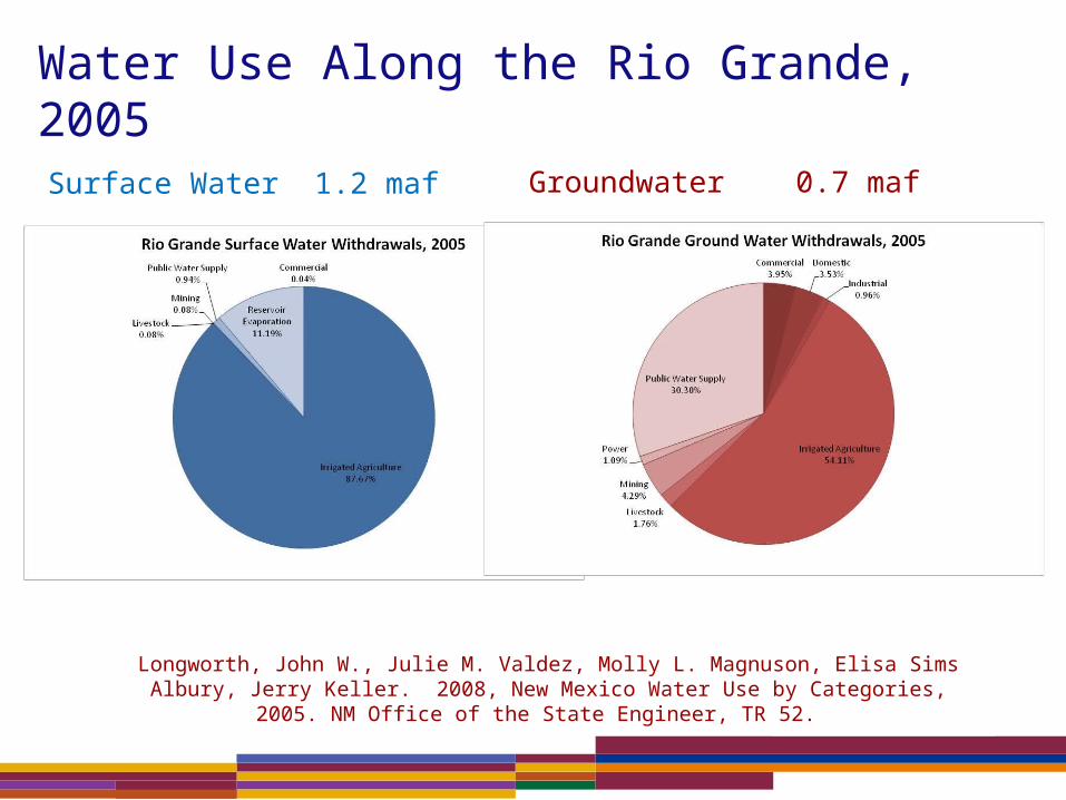
Water Use Along the Rio Grande, 2005
Longworth, John W., Julie M. Valdez, Molly L. Magnuson, Elisa Sims Albury, Jerry Keller. 2008, New Mexico Water Use by Categories, 2005. NM Office of the State Engineer, TR 52.
Surface Water 1.2 maf Groundwater 0.7 maf


Timing and Mixture of Surface and Groundwater in El Paso

Rio Grande Drought: Elephant Butte Reservoir (1) 89% June 2, 1994 (2) 3% July 8, 2013
source: http://climate.nasa.gov/state_of_flux#Elephant_Butte_930x607.jpg
Climate Change or Climate Variability
Watershed Assessment Goals and Objectives• Describe the important hydrological, bio-physical, economic, and institutional
characteristics at appropriate spatial and temporal scales
• Identify and characterize plausible alternative environmental and management scenarios and/or system changes
• Assess, analyze and describe the bio-physical and economic consequences of modeled scenarios and changes in environment, management, technology, infrastructure etc.
Models are tools that help plannersexamine data integrate concernsanalyze alternativesevaluate outcomes

Objectives of Hydro-Economic Watershed Models
• Represent major spatial, physical, and economic characteristics of water supply and use
• Evaluate welfare, allocation, and implicit price changes associated with alternative hydrologic, management, and institutional conditions
• Identify opportunities to improve water management systems from a watershed perspective
Hydro-Economic Modeling Basics
• Develop a schematic diagram of the watershed system– Describes physical structure (tributaries, inflows, and
reservoirs– Identifies and locates watershed services – Show diversion points and instream uses
• Derive estimates for the model’s objective function– Develop demand and supply curves for each service
based on water diversion or instream flow• Describe model constraints
– Mass balance (upstream to downstream flow)– Intertemporal storage in reservoirs– Institutional flow restrictions

Rio Grande Hydro-Economic Model Schematic Diagram

Model Objective FunctionGiven water supply, expected streamflows, and water demands in the watershed, the model objective is to choose (manage) all water diversions (allocations), reservoir storage and releases in order to:
Maximize present value of total long-run net economic welfare ($) defined as the sum of all net benefits less the sum of all costs and damages
( ) ( ) ( ) ( ) ( ) ( )t nit nit nit nit nt nt nt nt nt nt nt nt
t n i
PVNB d B W C W Q S H R E F D F
where Bint and Cnit define benefits and costs as a function of diverted water Wnit, Qnt and Hnt generate value from water stored Snt and released Rnt, Ent environmental services and flood damages Dnt are functions of flow Fnt.

Model Constraints: River Flow Mass Balance
Instream Flow Balance at each node (n) models the contemporaneous flow, storage and distribution of water.
where streamflow Fnt equals previous streamflow Fn-1,t plus additional rainfall and tributary inflow Int, net reservoir-release Rnt, upstream return-flow rni, and less diversions Wnit.
1, 1,n t nt nt ni n it nitnti
F F I R r W W

Model Constraints: Reservoir Storage Mass Balance
Reservoir (aquifer) Storage Balance for each time period (t):
where storage Snt equals previous period storage Sn,t-1 plus net additions from inflow Int and net-seepage from upstream diversions nniWn-1,it, less net amounts pumped or released Rnt and evaporation losses Lnt.
, 1 1,nt n t nt ni n it nt nt
i
S S I n W R L

Drought Damages
WB1 WA1
P1
W1 (drought)
WB0 WA0
P0
W0 (normal)
NBT
NBB
NBA
$($/m3)
Water
A Two-Sector Model of Efficient Water Distribution, Use and Drought Damages
Note: NB1 and NB2 are marginal net benefit curves that illustrate marginal benefits for water (water demand) after all associated marginal costs (e.g., conveyance, treatment, distribution) have been subtracted.

Water Demand Estimation
• A basic inverse linear water demand function:
• Pw = b0 + b1 Qw + b2 Z
• Pw = unit price of water ($/m3)
• Qw = quantity of water consumed (volumetric units e.g., m3)
• Z = other important factor(s) – could be several. E.g., land quality, seasons, irrigation technology.
• b0, b1 and b2 = parameters to be estimated
• Estimating water demand functions

Simple Water Demand Model
• With minimal data – i.e., a single data point and an estimate of the price-elasticity of water demand – a water demand function can still be approximated.
Example:
• Total annual sector water use = 250 MCM
• Estimated water value or price (marginal value of water) = $20 / MCM
• Estimate of price elasticity of demand in sector = 1.5

Elasticity: In Mathematical Notation
0
01
0
01
)(
)(
%
%
PPP
QQQ
Pchange
Qchange
Where: E is the elasticity of Q with respect to PQ1 is the new level of QQ0 is the old level of Qditto for P

Estimate Linear Demand Parameters: b0 and b1
• Linear demand function: Pw = b0 + b1 Qw
• Recall definitions:– ε = (Δ Q / Δ P) * (P0 / Q0)
– b1 = (P1 – P0) / (Q1 – Q0 )
• Data: P0, Q0, and ε
• Therefore, parameter are estimated as:– b1 = 1/ε * P0 / Q0 question: what should be the sign of b1?)
– b0 = P0 * (1 – 1 / ε)
•

Merci’ Beaucoup!GrazieThank YouGracias
Brian H. Hurd, PhDDepartment of Agricultural Economics & Agricultural BusinessGerald Thomas Hall Rm. 350New Mexico State UniversityTel : (575) 646-2674Email: [email protected]: http://agecon.nmsu.edu/bhurd