Embed Size (px)
Citation preview
Oracle® Data MiningConcepts
10g Release 1 (10.1)
Part No. B10698-01
December 2003
Oracle Data Mining Concepts, 10g Release 1 (10.1)
Part No. B10698-01
Copyright © 2003 Oracle. All rights reserved.
Primary Authors: Margaret Taft, Ramkumar Krishnan, Mark Hornick, Denis Mukhin, George Tang, Shiby Thomas.
Contributors: Charlie Berger, Marcos Campos, Boriana Milenova, Pablo Tamayo, Gina Abeles, Joseph Yarmus, Sunil Venkayala.
The Programs (which include both the software and documentation) contain proprietary information of Oracle Corporation; they are provided under a license agreement containing restrictions on use and disclosure and are also protected by copyright, patent and other intellectual and industrial property laws. Reverse engineering, disassembly or decompilation of the Programs, except to the extent required to obtain interoperability with other independently created software or as specified by law, is prohibited.
The information contained in this document is subject to change without notice. If you find any problems in the documentation, please report them to us in writing. Oracle Corporation does not warrant that this document is error-free. Except as may be expressly permitted in your license agreement for these Programs, no part of these Programs may be reproduced or transmitted in any form or by any means, electronic or mechanical, for any purpose, without the express written permission of Oracle Corporation.
If the Programs are delivered to the U.S. Government or anyone licensing or using the programs on behalf of the U.S. Government, the following notice is applicable:
Restricted Rights Notice Programs delivered subject to the DOD FAR Supplement are "commercial computer software" and use, duplication, and disclosure of the Programs, including documentation, shall be subject to the licensing restrictions set forth in the applicable Oracle license agreement. Otherwise, Programs delivered subject to the Federal Acquisition Regulations are "restricted computer software" and use, duplication, and disclosure of the Programs shall be subject to the restrictions in FAR 52.227-19, Commercial Computer Software - Restricted Rights (June, 1987). Oracle Corporation, 500 Oracle Parkway, Redwood City, CA 94065.
The Programs are not intended for use in any nuclear, aviation, mass transit, medical, or other inherently dangerous applications. It shall be the licensee's responsibility to take all appropriate fail-safe, backup, redundancy, and other measures to ensure the safe use of such applications if the Programs are used for such purposes, and Oracle Corporation disclaims liability for any damages caused by such use of the Programs.
Oracle is a registered trademark, and PL/SQL and SQL*Plus are trademarks or registered trademarks of Oracle Corporation. Other names may be trademarks of their respective owners.
iii
Contents
Send Us Your Comments ................................................................................................................... ix
Preface............................................................................................................................................................ xi
1 Introduction to Oracle Data Mining
1.1 What is Data Mining? ........................................................................................................... 1-11.2 What Is Oracle Data Mining? .............................................................................................. 1-11.2.1 Oracle Data Mining Programming Interfaces............................................................ 1-21.2.2 ODM Data Mining Functions....................................................................................... 1-2
2 Data for Oracle Data Mining
2.1 ODM Data, Cases, and Attributes....................................................................................... 2-12.2 ODM Data Requirements..................................................................................................... 2-22.2.1 ODM Data Table Format............................................................................................... 2-22.2.1.1 Single-Record Case Data........................................................................................ 2-22.2.1.2 Multi-Record Case Data in the Java Interface..................................................... 2-32.2.1.3 Wide Data in DBMS_DATA_MINING................................................................ 2-32.2.2 Column Data Types Supported by ODM................................................................... 2-52.2.2.1 Unstructured Data in ODM................................................................................... 2-52.2.2.2 Dates in ODM.......................................................................................................... 2-52.2.3 Attribute Type for Oracle Data Mining ...................................................................... 2-62.2.3.1 Target t Attribute .................................................................................................... 2-72.2.4 Data Storage Issues ........................................................................................................ 2-72.2.5 Missing Values in ODM ................................................................................................ 2-7
iv
2.2.5.1 Missing Values and Null Values in ODM ........................................................... 2-72.2.5.2 Missing Values Handling....................................................................................... 2-72.2.6 Sparse Data in Oracle Data Mining ............................................................................. 2-82.2.7 Outliers and Oracle Data Mining................................................................................. 2-82.3 Prepared and Unprepared Data ........................................................................................ 2-102.3.1 Data Preparation for the ODM Java Interface.......................................................... 2-102.3.2 Data Preparation for DBMS_DATA_MINING ........................................................ 2-102.3.3 Binning (Discretization) in Data Mining................................................................... 2-102.3.3.1 Methods for Computing Bin Boundaries .......................................................... 2-112.3.4 Normalization in Oracle Data Mining ...................................................................... 2-12
3 Predictive Data Mining Models
3.1 Classification .......................................................................................................................... 3-13.1.1 Costs ................................................................................................................................. 3-23.1.2 Priors ................................................................................................................................ 3-33.1.3 Naive Bayes Algorithm ................................................................................................. 3-33.1.4 Adaptive Bayes Network Algorithm........................................................................... 3-43.1.4.1 ABN Model Types................................................................................................... 3-53.1.4.2 ABN Rules ................................................................................................................ 3-53.1.4.3 ABN Build Parameters ........................................................................................... 3-63.1.4.4 ABN Model States ................................................................................................... 3-83.1.5 Comparison of NB and ABN Models.......................................................................... 3-83.1.6 Support Vector Machine................................................................................................ 3-93.1.6.1 Data Preparation and Settings Choice for Support Vector Machines ............. 3-93.2 Regression............................................................................................................................. 3-103.2.1 SVM Algorithm for Regression .................................................................................. 3-103.3 Attribute Importance .......................................................................................................... 3-103.3.1 Minimum Descriptor Length...................................................................................... 3-113.4 ODM Model Seeker (Java Interface Only) ....................................................................... 3-12
4 Descriptive Data Mining Models
4.1 Clustering in Oracle Data Mining ....................................................................................... 4-14.1.1 Enhanced k-Means Algorithm ..................................................................................... 4-24.1.1.1 Data for k-Means ..................................................................................................... 4-44.1.1.2 Scalability through Summarization...................................................................... 4-5
v
4.1.1.3 Scoring (Applying Models) ................................................................................... 4-54.1.2 Orthogonal Partitioning Clustering (O-Cluster) ....................................................... 4-54.1.2.1 O-Cluster Data Use ................................................................................................. 4-64.1.2.2 Binning for O-Cluster ............................................................................................. 4-64.1.2.3 O-Cluster Attribute Type....................................................................................... 4-64.1.2.4 O-Cluster Scoring.................................................................................................... 4-64.1.3 K-Means and O-Cluster Comparison.......................................................................... 4-74.2 Association Models in Oracle Data Mining....................................................................... 4-74.2.1 Finding Associations Involving Rare Events ............................................................. 4-84.2.2 Finding Associations in Dense Data Sets.................................................................... 4-94.2.3 Data for Association Models ........................................................................................ 4-94.2.4 Apriori Algorithm........................................................................................................ 4-104.3 Feature Extraction in Oracle Data Mining....................................................................... 4-104.3.1 Non-Negative Matrix Factorization .......................................................................... 4-114.3.1.1 NMF for Text Mining ........................................................................................... 4-11
5 Data Mining Using the Java Interface
5.1 Building a Model ................................................................................................................... 5-25.2 Testing a Model ..................................................................................................................... 5-35.2.1 Computing Lift ............................................................................................................... 5-35.3 Applying a Model (Scoring) ................................................................................................ 5-45.4 Model Export and Import .................................................................................................... 5-5
6 Objects and Functionality in the Java Interface
6.1 Physical Data Specification .................................................................................................. 6-16.2 Mining Function Settings ..................................................................................................... 6-16.3 Mining Algorithm Settings .................................................................................................. 6-26.4 Logical Data Specification.................................................................................................... 6-36.5 Mining Attributes.................................................................................................................. 6-36.6 Data Usage Specification...................................................................................................... 6-46.6.1 ODM Attribute Names and Case................................................................................. 6-46.7 Mining Model ........................................................................................................................ 6-46.8 Mining Results ....................................................................................................................... 6-56.9 Confusion Matrix................................................................................................................... 6-56.10 Mining Apply Output........................................................................................................... 6-6
vi
7 Data Mining Using DBMS_DATA_MINING
7.1 DBMS_DATA_MINING Application Development........................................................ 7-17.2 Building DBMS_DATA_MINING Models ........................................................................ 7-27.2.1 DBMS_DATA_MINING Models ................................................................................. 7-27.2.2 DBMS_DATA_MINING Mining Functions ............................................................... 7-27.2.3 DBMS_DATA_MINING Mining Algorithms ............................................................ 7-27.2.4 DBMS_DATA_MINING Settings Table...................................................................... 7-37.2.4.1 DBMS_DATA_MINING Prior Probabilities Table ............................................ 7-47.2.4.2 DBMS_DATA_MINING Cost Matrix Table........................................................ 7-57.3 DBMS_DATA_MINING Mining Operations and Results .............................................. 7-57.3.1 DBMS_DATA_MINING Build Results ....................................................................... 7-67.3.2 DBMS_DATA_MINING Apply Results ..................................................................... 7-67.3.3 Evaluating DBMS_DATA_MINING Classification Models .................................... 7-67.3.3.1 Confusion Matrix .................................................................................................... 7-77.3.3.2 Lift ............................................................................................................................. 7-87.3.3.3 Receiver Operating Characteristics ...................................................................... 7-87.3.4 Test Results for DBMS_DATA_MINING Regression Models............................... 7-107.3.4.1 Root Mean Square Error....................................................................................... 7-107.3.4.2 Mean Absolute Error ............................................................................................ 7-117.4 DBMS_DATA_MINING Model Export and Import ...................................................... 7-11
8 Text Mining Using Oracle Data Mining
8.1 What Text Mining Is.............................................................................................................. 8-18.1.1 Document Classification................................................................................................ 8-28.1.2 Combining Text and Numerical Data ......................................................................... 8-28.2 ODM Technologies Supporting Text Mining.................................................................... 8-28.2.1 Classification and Text Mining..................................................................................... 8-38.2.2 Clustering and Text Mining.......................................................................................... 8-38.2.3 Feature Extraction and Text Mining............................................................................ 8-48.2.4 Association and Regression and Text Mining............................................................ 8-48.3 Oracle Support for Text Mining .......................................................................................... 8-4
9 Oracle Data Mining Scoring Engine
9.1 Oracle Data Mining Scoring Engine Features ................................................................... 9-1
vii
9.2 Data Mining Scoring Engine Installation........................................................................... 9-19.3 Scoring in Data Mining Applications................................................................................. 9-19.4 Moving Data Mining Models .............................................................................................. 9-29.4.1 PMML Export and Import ............................................................................................ 9-29.4.2 Native ODM Export and Import.................................................................................. 9-29.5 Using the Oracle Data Mining Scoring Engine ................................................................. 9-3
10 Sequence Similarity Search and Alignment (BLAST)
10.1 Bioinformatics Sequence Search and Alignment............................................................ 10-110.2 BLAST in the Oracle Database .......................................................................................... 10-210.3 Oracle Data Mining Sequence Search and Alignment Capabilities............................. 10-2
A ODM Interface Comparison
A.1 Target Users of the ODM Interfaces ................................................................................... A-1A.2 Feature Comparison of the ODM Interfaces ..................................................................... A-2A.3 The ODM Interfaces in Different Programming Environments..................................... A-4
Glossary
Index

viii
ix
Send Us Your Comments
Oracle Data Mining Concepts, 10g Release 1 (10.1)
Part No. B10698-01
Oracle Corporation welcomes your comments and suggestions on the quality and usefulness of this document. Your input is an important part of the information used for revision.
■ Did you find any errors?■ Is the information clearly presented?■ Do you need more information? If so, where?■ Are the examples correct? Do you need more examples?■ What features did you like most?
If you find any errors or have any other suggestions for improvement, please indicate the document title and part number, and the chapter, section, and page number (if available). You can send com-ments to us in the following ways:
■ Electronic mail: [email protected] ■ FAX: 781-238-9893 Attn: Oracle Data Mining Documentation■ Postal service:
Oracle Corporation Oracle Data Mining Documentation10 Van de Graaff DriveBurlington, Massachusetts 01803U.S.A.
If you would like a reply, please give your name, address, telephone number, and (optionally) elec-tronic mail address.
If you have problems with the software, please contact your local Oracle Support Services.

x
xi
Preface
This manual discusses the basic concepts underlying Oracle Data Mining (ODM). Details of programming with the Java and PL/SQL interfaces are presented in the Oracle Data Mining Application Developer’s Guide.
Intended AudienceThis manual is intended for anyone planning to write data mining programs using the Oracle Data Mining interfaces. Familiarity with Java, PL/SQL, databases, and data mining is assumed.
StructureThis manual is organized as follows:
■ Chapter 1, "Introduction to Oracle Data Mining"
■ Chapter 2, "Data for Oracle Data Mining"
■ Chapter 3, "Predictive Data Mining Models"
■ Chapter 4, "Descriptive Data Mining Models"
■ Chapter 5, "Data Mining Using the Java Interface"
■ Chapter 6, "Objects and Functionality in the Java Interface"
■ Chapter 7, "Data Mining Using DBMS_DATA_MINING"
■ Chapter 8, "Text Mining Using Oracle Data Mining"
■ Chapter 9, "Oracle Data Mining Scoring Engine"
■ Chapter 10, "Sequence Similarity Search and Alignment (BLAST)"
xii
■ Appendix A, "ODM Interface Comparison"
■ Glossary
Sample applications and detailed uses cases are provided in the Oracle Data Mining Application Developer’s Guide.
Where to Find More InformationThe documentation set for Oracle Data Mining is part of the Oracle Database 10g Documentation Library. The ODM documentation set consists of the following documents, available online:
■ Oracle Data Mining Administrator’s Guide, 10g Release 1 (10.1)
■ Oracle Data Mining Concepts, 10g Release 1 (10.1) (this document)
■ Oracle Data Mining Application Developer’s Guide, 10g Release 1 (10.1)
Last-minute information about ODM is provided in the platform-specific release notes or README files.
For detailed information about the ODM Java interface, see the ODM Javadoc documentation in the directory $ORACLE_HOME/dm/doc/jdoc (UNIX) or %ORACLE_HOME%\dm\doc\jdoc (Windows) on any system where ODM is installed.
For detailed information about the PL/SQL interface, see the Supplied PL/SQL Packages and Types Reference.
For information about the data mining process in general, independent of both industry and tool, a good source is the CRISP-DM project (Cross-Industry Standard Process for Data Mining) (http://www.crisp-dm.org/).
Related ManualsFor more information about the database underlying Oracle Data Mining, see:
■ Oracle Administrator’s Guide, 10g Release 1 (10.1)
■ Oracle Database Installation Guide for your platform.
For information about developing applications to interact with the Oracle Database, see
■ Oracle Application Developer’s Guide — Fundamentals, 10g Release 1 (10.1)
xiii
For information about upgrading from Oracle Data Mining release 9.0.1 or release 9.2.0, see
■ Oracle Database Upgrade Guide, 10g Release 1 (10.1)
■ Oracle Data Mining Administrator’s Guide, 10g Release 1 (10.1)
For information about installing Oracle Data Mining, see
■ Oracle Installation Guide, 10g Release 1 (10.1)
■ Oracle Data Mining Administrator’s Guide, 10g Release 1 (10.1)
ConventionsIn this manual, Windows refers to the Windows 95, Windows 98, Windows NT, Windows 2000, and Windows XP operating systems.
The SQL interface to Oracle is referred to as SQL. This interface is the Oracle implementation of the SQL standard ANSI X3.135-1992, ISO 9075:1992, commonly referred to as the ANSI/ISO SQL standard or SQL92.
In examples, an implied carriage return occurs at the end of each line, unless otherwise noted. You must press the Return key at the end of a line of input.
The following conventions are also followed in this manual:
Convention Meaning
. . .
Vertical ellipsis points in an example mean that information not directly related to the example has been omitted.
. . . Horizontal ellipsis points in statements or commands mean that parts of the statement or command not directly related to the example have been omitted
boldface Boldface type in text indicates the name of a class or method.
italic text Italic type in text indicates a term defined in the text, the glossary, or in both locations.
typewriter In interactive examples, user input is indicated by bold typewriter font, and system output by plain typewriter font.
typewriter Terms in italic typewriter font represent placeholders or variables.
< > Angle brackets enclose user-supplied names.
xiv
Documentation Accessibility
Documentation Accessibility Our goal is to make Oracle products, services, and supporting documentation accessible, with good usability, to the disabled community. To that end, our documentation includes features that make information available to users of assistive technology. This documentation is available in HTML format, and contains markup to facilitate access by the disabled community. Standards will continue to evolve over time, and Oracle Corporation is actively engaged with other market-leading technology vendors to address technical obstacles so that our documentation can be accessible to all of our customers. For additional information, visit the Oracle Accessibility Program Web site at http://www.oracle.com/accessibility/.
Accessibility of Code Examples in DocumentationJAWS, a Windows screen reader, may not always correctly read the code examples in this document. The conventions for writing code require that closing braces should appear on an otherwise empty line; however, JAWS may not always read a line of text that consists solely of a bracket or brace.
[ ] Brackets enclose optional clauses from which you can choose one or none
Convention Meaning
Introduction to Oracle Data Mining 1-1
1Introduction to Oracle Data Mining
This chapter describes what data mining is, what Oracle Data Mining is, and outlines the data mining process.
1.1 What is Data Mining?Too much data and not enough information — this is a problem facing many businesses and industries.
A solution lies here, with data mining. Most businesses have an enormous amount of data, with a great deal of information hiding within it, but "hiding" is usually exactly what it is doing: So much data exists that it overwhelms traditional methods of data analysis.
Data mining provides a way to get at the information buried in the data. Data mining finds hidden patterns in large, complex collections of data, patterns that elude traditional statistical approaches to analysis.
1.2 What Is Oracle Data Mining?Oracle Data Mining (ODM) embeds data mining within the Oracle database. There is no need to move data out of the database into files for analysis and then back from files into the database for storing. The data never leaves the database — the data, data preparation, model building, and model scoring results all remain in the database. This enables Oracle to provide an infrastructure for application developers to integrate data mining seamlessly with database applications.
ODM is designed to support production data mining in the Oracle database. Production data mining is most appropriate for creating applications to solve problems such as customer relationship management, churn, etc., that is, any data mining problem for which you want to develop an application.
What Is Oracle Data Mining?
1-2 Oracle Data Mining Concepts
ODM provides single-user milt-session access to models. Model building is either synchronous in the PL/SQL interface or asynchronous in the Java interface.
1.2.1 Oracle Data Mining Programming InterfacesODM integrates data mining with the Oracle data base and exposes data mining through the following interfaces:
■ Java interface: Allows users to embed data mining in Java applications.
■ DBMS_DATA_MINING and DBMS_DATA_MINING_TRANSFORM: Allow users to embed data mining in PL/SQL applications.
The ODM Java interface and DBMS_DATA_MINING have similar, but not identical, capabilities. For a comparison of the interfaces, see Appendix A.
1.2.2 ODM Data Mining FunctionsData mining functions are based on two kinds of learning: supervised (directed) and unsupervised (undirected).
Supervised learning functions are typically used to predict a value, and are sometimes referred to as predictive models. Unsupervised learning functions are typically used to find the intrinsic structure, relations, or affinities in data but no classes or labels are assigned aprioi. These are sometimes referred to as descriptive models.
Oracle Data Mining supports the following data mining functions:
■ Predictive models (supervised learning):
– Classification: grouping items into discrete classes and predicting which class an item belongs to
– Regression: function approximation and forecast of continuous values
– Attribute importance: identifying the attributes that are most important in predicting results (Java interface only)
■ Descriptive models (unsupervised learning):
Note: The Java and PL/SQL interfaces do not produce models that are interoperable. For example, you cannot produce a model with Java and apply it using PL/SQL, or vice versa, in this release.
What Is Oracle Data Mining?
Introduction to Oracle Data Mining 1-3
– Clustering: finding natural groupings in the data
– Association models: "market basket" analysis
– Feature extraction: create new attributes (features) as a combination of the original attributes
■ Multimedia (TEXT)
■ Bioinformatics (BLAST)

What Is Oracle Data Mining?
1-4 Oracle Data Mining Concepts
Data for Oracle Data Mining 2-1
2Data for Oracle Data Mining
This chapter describes data requirements and how the data is to be prepared before you can begin mining it using either of the Oracle Data Mining (ODM) interfaces. The data preparation required depends on the type of model that you plan to build and the characteristics of the data. For example data that only takes on a small number of values may not require binning.
The following topics are addressed:
■ Data, cases, and attributes
■ Data Requirements
■ Data Format
■ Attribute Type
■ Missing Values
■ Prepared and unprepared data
■ Normalizing
■ Binning
2.1 ODM Data, Cases, and AttributesData used by ODM consists of tables stored in an Oracle database. The rows of a data table are referred to as cases, records, or examples. The columns of the data tables are referred to as attributes (also known as fields); each attribute in a record holds an item of information. The attribute names are constant from record to record; the values in the attributes can vary from record to record. For example, each record may have an attribute labeled "annual income". The value in the annual income attribute can vary from one record to another.
ODM Data Requirements
2-2 Oracle Data Mining Concepts
ODM distinguishes two types of attributes: categorical and naumerical. Categorical attributes are those that define their values as belonging to a small number of discrete categories or classes; there is no implicit order associated with them. If there are only two possible values, for example yes and no, or male and female, the attribute is said to be binary. If there are more than two possible values, for example, small, medium, large, extra large, the attribute is said to be multiclass.
Numerical attributes are those that take on continuous values, for example, annual income or age. Annual income or age could theoretically be any value from zero to infinity, though of course in practice each usually occupies a more realistic range.
Numerical attributes can be treated as categorical: Annual income, for example, could be divided into three categories: low, medium, high.
Certain ODM algorithms also support unstructured attributes. Currently only one type of unstructured attribute type Text is supported. At most one attribute of type Text is allowed in ODM data.
2.2 ODM Data RequirementsODM has requirements on several aspects of input data: data table format, column data type, and attribute type.
2.2.1 ODM Data Table FormatODM data can be in one of two formats:
■ Single-record case (also known as nontransactional; these are ordinary relational tables)
■ Multi-record case (also know as transactional), used for data with many attributes (DBMS_DATA_MINING uses nested tables; see Section 2.2.1.3.)
The Java interface for ODM provides a transformation utility reversePivot() that converts multiple data sources that are in single-record case format to one table that is in multi-record case format. Reverse pivoting can be used to create tables that exceed the 1000 column limit on Oracle tables by combining multiple tables that have a common key.
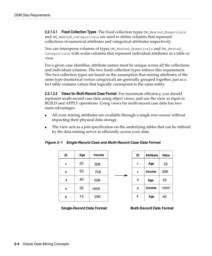
2.2.1.1 Single-Record Case DataIn single-record case (nontransactional) format, each case is stored as one row in a table. Single-record-case data is not required to provide a key column to uniquely
ODM Data Requirements
Data for Oracle Data Mining 2-3
identify each record. However, a key is needed to associate cases with resulting scores for supervised learning. This format is also referred to as nontransactional.
Note that certain algorithms in the ODM Java interface automatically and internally (that is, in a way invisible to the user) convert all single-record case data to multi-record case data prior to model building. If data is already in multi-record case format, algorithm performance might be enhanced over performance with data in single-record case format.
2.2.1.2 Multi-Record Case Data in the Java InterfaceOracle tables support at most 1,000 columns. This means that a case can have at most 1,000 attributes. Data that has more than 1,000 attributes is said to be wide. Certain classes of problems, especially problems in Bioinformatics, are associated with wide data.
The Java interface requires that wide data be in multi-record case format.
In multi-record case data format, each case is stored as multiple records (rows) in a table with columns sequence ID, attribute name, and value (these are user-defined names). This format is also referred to as transactional.
SequenceID is an INTEGER or NUMBER that associates the records that make up a single case in a multi-record case table, attribute name is a string containing the name of the attribute, and value is a number representing the value of the attribute. Note that the values in the value column must be of type NUMBER; non-numeric data must be converted to numeric data, usually by binning or explosion.
2.2.1.3 Wide Data in DBMS_DATA_MININGIn the domains of bioinformatics, text mining, and other specialized areas, the data is wide and shallow — relatively few cases, but with one thousand or more mining attributes.
Wide data can be represented in a multi-record case format, where attribute/value pairs are grouped into collections (nested tables) associated with a given case ID. Each row in the multi-record collection represents an attribute name (and its corresponding value in another column in the nested table).
DBMS_DATA_MINING includes fixed collection types for defining columns.
It is most efficient to represent multi--record case data as a view.
ODM Data Requirements
2-4 Oracle Data Mining Concepts
2.2.1.3.1 Fixed Collection Types The fixed collection types DM_Nested_Numericals and DM_Nested_Categoricals are used to define columns that represent collections of numerical attributes and categorical attributes respectively.
You can intersperse columns of types DM_Nested_Numericals and DM_Nested_Categoricals with scalar columns that represent individual attributes in a table or view.
For a given case identifier, attribute names must be unique across all the collections and individual columns. The two fixed collection types enforce this requirement. The two collection types are based on the assumption that mining attributes of the same type (numerical versus categorical) are generally grouped together, just as a fact table contains values that logically correspond to the same entity.
2.2.1.3.2 Views for Multi-Record Case Format For maximum efficiency, you should represent multi-record case data using object views, and use the view as input to BUILD and APPLY operations. Using views for multi-record case data has two main advantages:
■ All your mining attributes are available through a single row-source without impacting their physical data storage.
■ The view acts as a join specification on the underlying tables that can be utilized by the data mining server to efficiently access your data.
Figure 2–1 Single-Record Case and Multi-Record Case Data Format
ODM Data Requirements
Data for Oracle Data Mining 2-5
2.2.2 Column Data Types Supported by ODMODM does not support all the data types that Oracle supports. ODM attributes must have one of the following data types:
■ VARCHAR2
■ CHAR
■ NUMBER
■ CLOB
■ BLOB
■ BFILE
■ XMLTYPE
■ URITYPE
The supported attribute data types have a default attribute type (categorical or numerical); Table 2–1 lists the default attribute type for each of these data types.
2.2.2.1 Unstructured Data in ODMSome ODM algorithms (Support Vector Machine, Non-Negative Matrix Factorization, Association, and the implementation of k-means Clustering in DBMS_DATA_MINING) permit one column to be unstructured of type Text. For information about text mining, see Chapter 8.
2.2.2.2 Dates in ODMODM does not support the DATE data type. Depending on the meaning of the item, you convert items of type DATE to either type VARCHAR2 or NUMBER.
If, for example, the date serves as a timestamp indicating when a transaction occurred, converting the date to VARCHAR2 makes it categorical with unique values, one per record. These types of columns are known as "identifiers" and are not useful in model building. However, if the date values are coarse and significantly fewer than the number of records, this mapping may be fine.
One way to convert a date to a number is as follows: select a starting date and subtract the starting date from each date value. This result produces a NUMBER column, which can be treated as a numerical attribute, and then binned as necessary.
ODM Data Requirements
2-6 Oracle Data Mining Concepts
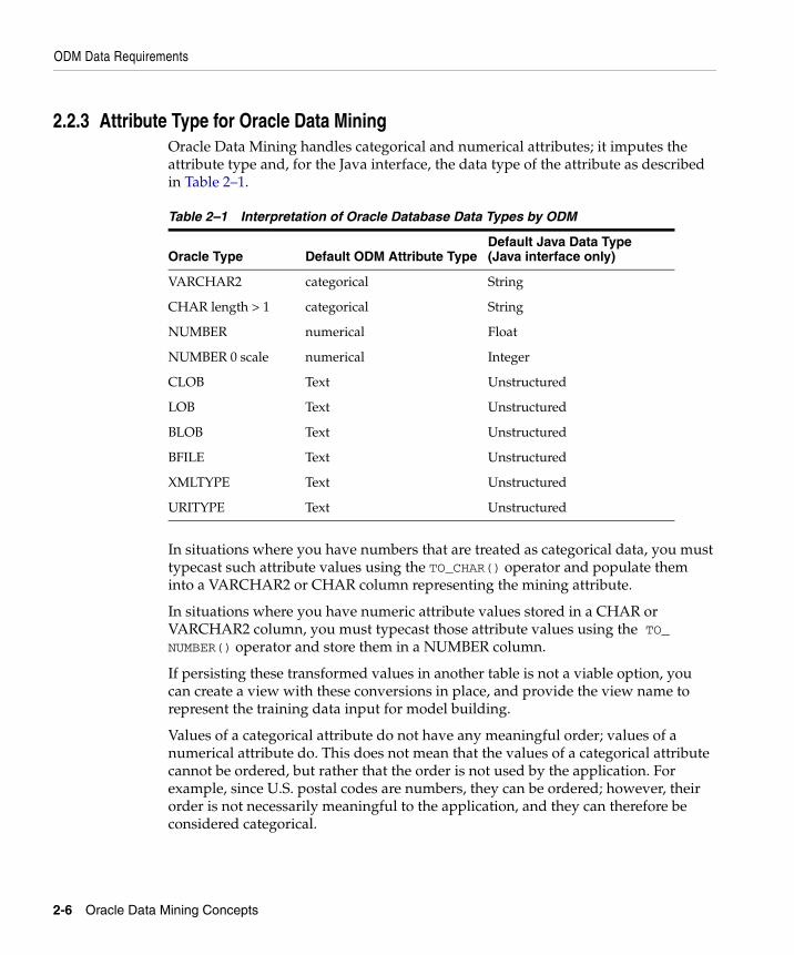
2.2.3 Attribute Type for Oracle Data MiningOracle Data Mining handles categorical and numerical attributes; it imputes the attribute type and, for the Java interface, the data type of the attribute as described in Table 2–1.
In situations where you have numbers that are treated as categorical data, you must typecast such attribute values using the TO_CHAR() operator and populate them into a VARCHAR2 or CHAR column representing the mining attribute.
In situations where you have numeric attribute values stored in a CHAR or VARCHAR2 column, you must typecast those attribute values using the TO_NUMBER() operator and store them in a NUMBER column.
If persisting these transformed values in another table is not a viable option, you can create a view with these conversions in place, and provide the view name to represent the training data input for model building.
Values of a categorical attribute do not have any meaningful order; values of a numerical attribute do. This does not mean that the values of a categorical attribute cannot be ordered, but rather that the order is not used by the application. For example, since U.S. postal codes are numbers, they can be ordered; however, their order is not necessarily meaningful to the application, and they can therefore be considered categorical.
Table 2–1 Interpretation of Oracle Database Data Types by ODM
Oracle Type Default ODM Attribute TypeDefault Java Data Type (Java interface only)
VARCHAR2 categorical String
CHAR length > 1 categorical String
NUMBER numerical Float
NUMBER 0 scale numerical Integer
CLOB Text Unstructured
LOB Text Unstructured
BLOB Text Unstructured
BFILE Text Unstructured
XMLTYPE Text Unstructured
URITYPE Text Unstructured
ODM Data Requirements
Data for Oracle Data Mining 2-7
2.2.3.1 Target t AttributeClassification and Regression algorithms require a target attribute. A DBMS_DATA_MINING predictive model can on predict a single target attribute. The target attribute for all classification algorithms can be numerical or categorical. SVM Regression supports only numerical target attributes.
2.2.4 Data Storage IssuesIf there are a few hundred mining attributes and your application requires the attributes to be represented as columns in the same row of the table, data storage must be carefully designed. For a table with several columns, the key question to consider is the (average) row length, not the number of columns. Having more than 255 columns in a table built with a smaller block size typically results in intrablock chaining. Oracle stores multiple row pieces in the same block, but the overhead to maintain the column information is minimal as long as all row pieces fit in a single data block. If the rows don't fit in a single data block, you may consider using a larger database block size (or use multiple block sizes in the same database). For more details, consult Oracle Database Concepts and Oracle Database Performance Tuning Guide.
2.2.5 Missing Values in ODMData tables often contain missing values.
2.2.5.1 Missing Values and Null Values in ODMThe following algorithms assume that a null values indicate missing values (and not as indicators of sparse data): NB, ABN, AI, k-Means (Java interface), and O-Cluster.
2.2.5.2 Missing Values HandlingODM is robust in handling missing values and does not require users to treat missing values in any special way. ODM will ignore missing values but will use non-missing data in a case.
In some situations you must be careful, for example, in transactional format, to distinguish between a "0" that has an assigned meaning and an empty cell.
Note: Do not confuse missing values with sparse data.
ODM Data Requirements
2-8 Oracle Data Mining Concepts
2.2.6 Sparse Data in Oracle Data MiningData is said to be sparse if only a small fraction (no more than 20%, often 3% or less) of the attributes are non-zero or non-null for any given case. Sparse data occurs, for example, in market basket problems. In a grocery store, there might be 10,000 products in the store, and the average size of a basket (the collection of distinct items that a customer purchases in a typical transaction) is 50 or fewer products. In this example, a transaction (case or record) has at most 50 out of 10,000 attributes that are not null. This implies that the fraction of non-zero attributes in the table (or the density) is 50/10,000, or 0.5%. This density is typical for market basket and text processing problems.
Association models are designed to process sparse data; indeed, if the data is not sparse, the algorithm may require a large amount of temporary space and may not be able to build a model.
Different algorithms make different assumptions about what indicates sparse data as follows:
■ Support Vector Machine, Non-Negative Matrix Factorization, k-Means in DBMS_DATA_MINING: NULL values indicate sparse data. Missing values are not automatically handled. If the data is not sparse and the values are indeed missing at random, it is necessary to perform missing data imputation (that is, perform some kind of missing values "treatment") and substitute the nulls value for a non-null value. One simple approach is to substitute the mean for numerical attributes and the mode for categorical attributes. If you do not treat missing values, the algorithm will not handle the data correctly.
■ All other algorithms (including k-Means in the Java interface): NULL values are treated as missing and not indicators of sparse data.
2.2.7 Outliers and Oracle Data MiningAn outlier is a value that is far outside the normal range in a data set, typically a value that is several standard deviations from the mean. The presence of outliers can have a significant impact on ODM models.
Outliers affect ODM during data pre-processing either when it is performed by the user or automatically during model build.
Outliers affect the different algorithms as follows:
■ Attribute Intelligence, Naive Bayes, Adaptive Bayes Network: The presence of outliers, when automatic data preparation or external equal-width bining is used, makes most of the data concentrate in a few bins (a single bin in extreme
ODM Data Requirements
Data for Oracle Data Mining 2-9
cases). As a result, the discriminating power of these algorithms may be significantly reduced. In the case of ABN, if all attributes have outliers, ABN may not even be able to build a tree beyond a first split.
■ Association Models: The presence of outliers, when automatic data preparation or external equal-width bining is used, makes most of the data concentrate in a few bins (a single bin in extreme cases). As a result, the ability of AR to detect differences in numerical attributes may be significantly lessened. For example, a numerical attribute such as income may have all the data belonging to a single bin except for one entry (the outlier) that belongs to a different bin. As a result, there won't be any rules reflecting different levels of income. All rules containing income will only reflect the range in the single bin; this range is basically the income range for the whole population
■ O-Cluster: The presence of outliers, when automatic data preparation or external equal-width bining is used, will make most of the data concentrate in a few bins (a single bin in extreme cases). As a result, the ability of O-Cluster to detect clusters may be significantly impacted. If the whole data is divided among a few bins, it may look as if there are no clusters, that is, that the whole population falls in a single cluster.
■ k-Means (Java interface): The presence of outliers, when automatic data preparation or external equal-width bining is used, will make most of the data concentrate in a few bins (a single bin in extreme cases). As a result, the ability of k-Means to create clusters that are different in content may be significantly impacted. If the whole data is divided among a few bins, then clusters may have very similar centroids, histograms, and rules.
■ k-Means (PL/SQL interface): The presence of outliers, when automatic data preparation or min-max normalization is used, will make most of the data concentrate in a small range. As a results the ability of k-Means to create clusters that are different in content may be significantly impacted. If the whole data is concentrated in a small range, then clusters may have very similar centroids, histograms, and rules.
■ Support Vector Machine: The presence of outliers, when automatic data preparation or min-max normalization is used, will make most of the data concentrate in a small range. As a result it will make learning harder and lead to longer training times.
■ Non-Negative Matrix Factorization: The presence of outliers, when automatic data preparation or min-max normalization is used, will make most of the data concentrate in a small range. This will result in poor matrix factorization in
Prepared and Unprepared Data
2-10 Oracle Data Mining Concepts
general. To improve the matrix factorization the error tolerance would need to be decreased. This in turn would lead to longer build times.
2.3 Prepared and Unprepared DataData is said to be prepared or unprepared, depending on whether certain data transformations required by a data mining algorithm were performed by the user.
For the Java interface, data can be either unprepared (the default) or prepared; data for DBMS_DATA_MINING must be prepared.
2.3.1 Data Preparation for the ODM Java InterfaceThe ODM Java interface assumes data is unprepared and automatically performs the transformations necessary to prepare the data. This means different things to different algorithms. For most of the algorithms ODM, prepared data is binned data. Unbinned data is said to be unprepared. See Section 2.3.3 for information about binning in the java interface.
For the SVM and NMF algorithms, prepared data is normalized data. See Section 2.3.4 for information about normalization.
The user can specify the data’s status (prepared or unprepared) in the DataPreparationStatus setting for each attribute. For example, if the user has already binned the data for an attribute, the data’s status for that attribute should be set to prepared using so that ODM will not bin the data for that attribute again. If the user wants ODM to do the binning for all attributes, the status should be set to unprepared for all attributes.
Support Vector Machine models require especially careful data preparation. For more information, see Section 3.1.6.1.
2.3.2 Data Preparation for DBMS_DATA_MININGThe PL/SQL interface assumes that all data is prepared. The user must perform any required data preparation.
2.3.3 Binning (Discretization) in Data MiningSome ODM algorithms may benefit from binning (discretizing) both numeric and categorical data. Naive Bayes, Adaptive Bayes Network, Clustering, Attribute Importance, and Association Rules algorithms may benefit from binning.
Prepared and Unprepared Data
Data for Oracle Data Mining 2-11
Binning means grouping related values together, thus reducing the number of distinct values for an attribute. Having fewer distinct values typically leads to a more compact model and one that builds faster, but it can also lead to some loss in accuracy.
2.3.3.1 Methods for Computing Bin Boundaries ODM utilities provide three methods for computing bin boundaries from the data:
■ Top N most frequent items: For categorical attributes only, the user selects the value N and the name of the "other" category. ODM determines the N most frequent values and puts all other values in the "other" category.
■ Equi-Width Binning: For numerical attributes, ODM finds min, max values for every attribute in the data. Then ODM divides the [min, max] range into N (specified by the user) equal regions of size d=(max-min)/N. Thus bin 1 is [min, min+d), bin 2 is [min+d, min+2d) and bin N is [min+(N-1)*d,max].
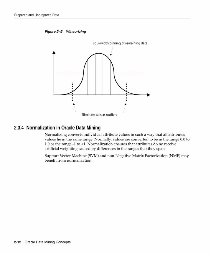
■ Equi-Width Binning with Winsorizing: The difference between equi-width binning and equi-width binning with winsorizing is in the computation of min and max values that are computed not on the original but on the winsorized data. Winsorizing is accomplished by ordering the data and then excluding the data points from the beginning and end of the ordered set. The number of data points excluded from both ends is specified as a percentage of non-NULL values in the column. For example, if there are 200 non-NULL values in the column and tail percentage = 1.5, then 6 data points in total are removed, 3 from each end (3 smallest and 3 largest). See Figure 2–2.
Prepared and Unprepared Data
2-12 Oracle Data Mining Concepts
Figure 2–2 Winsorizing
2.3.4 Normalization in Oracle Data MiningNormalizing converts individual attribute values in such a way that all attributes values lie in the same range. Normally, values are converted to be in the range 0.0 to 1.0 or the range -1 to +1. Normalization ensures that attributes do no receive artificial weighting caused by differences in the ranges that they span.
Support Vector Machine (SVM) and non-Negative Matrix Factorization (NMF) may benefit from normalization.
Predictive Data Mining Models 3-1
3Predictive Data Mining Models
This chapter describes the predictive models, that is, the supervised learning functions. These functions predict a target value. The Oracle Data Mining Java interface supports the following predictive functions and associated algorithms:
This chapter also describes ODM Model Seeker (Section 3.4), which builds several Naive Bayes and Adaptive Bayes Network models and selects the best one.
3.1 ClassificationIn a classification problem, you typically have historical data (labeled examples) and unlabeled examples. Each labeled example consists of multiple predictor attributes and one target attribute (dependent variable). The value of the target attribute is a class label. The unlabeled examples consist of the predictor attributes only. The goal of classification is to construct a model using the historical data that accurately predicts the label (class) of the unlabeled examples.
A classification task begins with build data (also know as training data) for which the target values (or class assignments) are known. Different classification algorithms use different techniques for finding relations between the predictor
Function Algorithm
Classification (Section 3.1) Naive Bayes (Section 3.1.3)
Adaptive Bayes Network (Section 3.1.4)
Support Vector Machine (Section 3.1.6)
Regression (Section 3.2) Support Vector Machine (Section 3.2.1)
Attribute Importance (Section 3.3)
Minimal Descriptor Length (Section 3.3.1)
Classification
3-2 Oracle Data Mining Concepts
attributes’ values and the target attribute's values in the build data. These relations are summarized in a model, which can then be applied to new cases with unknown target values to predict target values. A classification model can also be used on build data with known target values, to compare the predictions to the known answers; such data is also known as test data or evaluation data. This technique is called testing a model, which measures the model's predictive accuracy. The application of a classification model to new data is called applying the model, and the data is called apply data or scoring data. Applying data is often called scoring the data.
Classification is used in customer segmentation, business modeling, credit analysis, and many other applications. For example, a credit card company may wish to predict which customers will default on their payments. Each customer corresponds to a case; data for each case might consist of a number of attributes that describe the customer's spending habits, income, demographic attributes, etc. These are the predictor attributes. The target attribute indicates whether or not the customer has defaulted; that is, there are two possible classes, corresponding to having defaulted or not. The build data is used to build a model that you then use to predict, for new cases, whether these new customers are likely to default.
3.1.1 CostsIn a classification problem, it may be important to specify the costs involved in making an incorrect decision. Doing so can be useful when the costs of different misclassifications vary significantly.
For example, suppose the problem is to predict whether a user will respond to a promotional mailing. The target has two categories: YES (the customer responds) and NO (the customer does not respond). Suppose a positive response to the promotion generates $500 and that it costs $5 to do the mailing. If the model predicts YES and the actual value is YES, the cost of misclassification is $0. If the model predicts YES and the actual value is NO, the cost of misclassification is $5. If the model predicts NO and the actual value is YES, the cost of misclassification is $500. If the model predicts NO and the actual value is NO, the cost is $0.
The row indexes of a cost matrix correspond to actual values; the column indexes correspond to predicted values. For any pair of actual/predicted indexes, the value indicates the cost of misclassification.
Classification algorithms apply the cost matrix to the predicted probabilities during scoring to estimate the least expensive prediction. If a cost matrix is specified for apply, the output of the scoring run is prediction and cost., rather than predication and probability
Classification
Predictive Data Mining Models 3-3
3.1.2 PriorsIn building a classification model, priors can be useful when the training data does not accurately reflect the real underlying population. A priors vector is used to inform the model of the true underlying distribution of target classes in the underlying population. The model build adjusts its predicted probabilities for Adaptive Bayes Network and Naive Bayes or relative Complexity factor for Support Vector Machine.
3.1.3 Naive Bayes AlgorithmThe Naive Bayes algorithm (NB)N can be used for both binary and multiclass classification problems to answer questions such as "Which customers will switch to a competitor? Which transaction patterns suggest fraud? Which prospects will respond to an advertising campaign?" For example, suppose a bank wants to promote its mortgage offering to its current customers and that, to reduce promotion costs, it wants to target the most likely prospects. The bank has historical data for its customers, including income, number of household members, money-market holdings, and information on whether a customer has recently obtained a mortgage through the bank. Using NB, the bank can predict how likely a customer is to respond positively to a mortgage offering. With this information, the bank can reduce its promotion costs by restricting the promotion to the most likely candidates.
NB affords fast model building and scoring for relatively low volumes of data.
NB makes predictions using Bayes’ Theorem, which derives the probability of a prediction from the underlying evidence.Bayes’ Theorem states:
P(A | B) = (P(B | A) P(A))/P(B)
That is, the probability of event A occurring given that event B has occurred is equal to the probability of event B occurring given that event A has occurred, multiplied by the probability of event A occurring and divided by the probability of event B occurring.
NB assumes that each attribute is conditionally independent of the others: given a particular value of the target, the distribution of each predictor is independent of the other predictors.
In practice, this assumption, even when violated, does not degrade the model’s predictive accuracy significantly, and makes the difference between a fast, computationally feasible algorithm and an intractable one.
Classification
3-4 Oracle Data Mining Concepts
Naive Bayes lets you, using cross-validation, test model accuracy on the same data that was used to build the model, rather than building the model on one portion of the data and testing it on a different portion. Not having to hold aside a portion of the data for testing is especially useful if the amount of build data is relatively small.
"Leave-one-out cross-validation" is a special case of cross-validation in which one record is left out of the build data when building a model. The number of models built equals the number of records (omitting a different build record for each model), which makes this procedure computationally expensive. With Naive Bayes models, however, the approach can be modified such that all build records are used for building a single model. Then, the model is repeatedly modified to quickly remove the effects of one build record, incrementally "unbuilding" the model for that record, as though that record had been omitted when building the model in the first place. The accuracy of the prediction for each build record can then be assessed against the model that would have been built from all the build records except that one, without having had to actually build a separate model for each build record.
To use Naive Bayes cross-validation, the user executes a CrossValidate task object, specifying that a Naive Bayes model is to be tested. The execution of the cross-validate task creates a ClassificationTestResult associated with classification test metrics.
See Table 3–1, below, for a comparison of the main characteristics of ABN and NB.
3.1.4 Adaptive Bayes Network AlgorithmAdaptive Bayes Network (ABN) is an Oracle proprietary algorithm that provides a fast, scalable, non-parametric means of extracting predictive information from data with respect to a target attribute. (Non-parametric statistical techniques avoid assuming that the population is characterized by a family of simple distributional models, such as standard linear regression, where different members of the family are differentiated by a small set of parameters.)
ABN, in single feature build mode, can describe the model in the form of human-understandable rules. The rules produced by ABN are one of its main advantages over Naive Bayes. The business user, marketing professional, or business analyst can understand the basis of the model’s predictions and can therefore be comfortable acting on them and explaining them to others.
In addition to explanatory rules, ABN provides performance and scalability, which are derived via a collection of user parameters controlling the trade-off of accuracy and build time.
Classification
Predictive Data Mining Models 3-5
ABN predicts binary as well as multiclass targets. Binary targets are those that take on only two values, for example, buy and not buy. Multiclass targets have more than two values, for example, products purchased (product A or product B or product C). Multiclass target values are not assumed to exist in an ordered relation to each other, for example, hair brush is not assumed to be greater or less than comb.
ABN can use costs and priors for both building and scoring (see Section 3.1.1 and Section 3.1.2).
3.1.4.1 ABN Model TypesAn ABN model is an (adaptive conditional independence model that uses the minimum description length principle to construct and prune an array of conditionally independent Network Features. Each Network Feature consists of one or more Conditional Probability Expressions. The collection of Network Features forms a product model that provides estimates of the target class probabilities. There can be one or more Network Features. The number and depth of the Network Features in the model determine the model mode. There are three model modes for ABN:
■ Pruned Naive Bayes (Naive Bayes Build)
■ Simplified decision tree (Single Feature Build)
■ Boosted (Multi Feature Build)
Users can select the ABN model type. Rules are available only for Single Feature Build; see Section 3.1.4.2 for information about rules.
Each Network Feature consists of one or more attributes included in a Conditional Probability Expression. An array of single attribute Network Features is an MDL-pruned Naive Bayes model. A single multi-attribute Network Feature model is equivalent to a simplified C4.5 decision tree; such a model is simplified in the sense that numerical attributes are binned and treated as categorical. Furthermore, a single predictor is used to split all nodes at a given tree depth. The splits are k-way, where k is the number of unique (binned) values of the splitting predictor. Finally, a collection of multi-attribute Network Features forms a product model (boosted mode). All three types provide estimates of the target class probabilities.
3.1.4.2 ABN RulesRules can be extracted from the Adaptive Bayes Network Model as Compound Predicates. Rules form a human-interpretable depiction of the model and include statistics indicating the number of the relevant training data instances in support of
Classification
3-6 Oracle Data Mining Concepts
the rule. A record apply instance specifies a pathway in a network feature taking the form of a compound predicate.
For example, suppose the feature consists of two training attributes: Age {20-40, 40-60, 60-80} and Income {<=50K, >50K}. A record instance consisting of a person age 25 and income $42K is expressed as
IF AGE IN (20-40) and INCOME IN (<=50K)
Suppose that the associated target (for example, response to a promotion) probabilities are {0.8 (no), 0.2 (yes)}. Then we have a detailed rule of the form
IF AGE IN (20-40) and INCOME IN (<=50K) => Prob = {0.8, 0.2}
In addition to the probability distribution, there are the associated training data counts, e.g. {400, 100}. Suppose there is a cost matrix specifying that it is 6 times more costly to incorrectly predict a no than to incorrectly predict a yes. Then the cost of predicting yes for this instance is 0.8 * 1 = 0.8 (because the model is wrong in this prediction 80% of the time) and the cost of predicting no is 0.2 * 6 = 1.2. Thus, the minimum cost (best) prediction is yes.
Without the cost matrix and the decision is reversed. Implicitly, all errors are equal and we have: 0.8 * 1 = 0.8 for yes and 0.2 * 1 = 0.2 for no.
The order of the predicates in the generated rules implies relative importance.
When you apply an ABN model for which rules were generated, with a single feature, you get the same result that you would get if you wrote an external program that applied the rules.
3.1.4.3 ABN Build ParametersTo control the execution time of a build, ABN provides the following user-settable parameters:
■ MaximumNetworkFeatureDepth: NetworkFeatures are like individual decision trees. This parameter restricts the depth of any individual NetworkFeature in the model. At each depth for an individual NetworkFeature there is only one predictor chosen. Each level built requires an additional scan of the data, so the computational cost of deep feature builds is high. The range for this parameter consists of the positive integers. The NULL or 0 value setting has special meaning: unrestricted depth. Builds beyond depth 7 are rare. Default is 10.
■ MaximumConsecutivePrunedNetworkFeatures: The maximum number of consecutive pruned features before halting the stepwise selection process. Default is 1.
Classification
Predictive Data Mining Models 3-7
■ MaximumBuildTime: The maximum build time (in minutes) parameter allows the user build quick, possibly less accurate models for immediate use or simply to get a sense of how long it will take to build a model with a given set of data. To accomplish this, the algorithm divides the build into milestones (model states) representing complete functional models (see ABNModelBuildState for details). The algorithm completes at least a single milestone and then projects whether it can reach the next one within the user-specified maximum build time. This decision is revisited at each milestone achieved until either the model build is complete or the algorithm determines it cannot reach the next milestone within the user-specified time limit. The user has access to the statistics produced by the time estimation procedure (see ABNModelBuildState for details). Default is NULL (no time limit).
■ MaximumPredictors: The maximum number of predictors is a feature selection mechanism that can provide a substantial performance improvement, especially in the instance of training tables where the number of attributes is high (but less than 1000) and is represented in single-record format. Note that the predictors are rank ordered with respect to an MDL measure of their correlation to the target, which is a greedy measure of their likelihood of being incorporated into the model. Default is 25.
■ NumberPredictorsInNBModel: The number of predictors in the NB model. The actual number of predictors will be the minimum of the parameter value and the number of active predictors in the model. If the value is less than the number of active predictors in the model, the predictors are chosen in accordance with their MDL rank. Default is 10.
■ Model Types: You can specify one of the following types when building an ABN model:
– MultiFeatureBuild: The model search space includes an NB model and single and multi-feature product probability models. Rules are produced only if the single feature model is best. No rules are produced for multi-feature or NB models.
– SingleFeatureBuild: The model search space includes only a single feature model with one or more predictors. Rules are produced.
– NaiveBayesBuild: Only a single model is built, an NB model. It is compared with the global sample prior (the distribution of target values in the sample). If the NB model is a better predictor of the target values than the global prior, then the NB model is output. Otherwise no model is output. No rules are produced.
Note that only single feature model results in rules.
Classification
3-8 Oracle Data Mining Concepts
3.1.4.4 ABN Model StatesWhen you specify MaxBuildTime for a boosted mode ABN model, the ABN build terminates in one of the following states:
■ CompleteMultiFeature: Multiple features have been tested for inclusion in the model. MDL pruning has determined whether the model actually has one or more features. The model may have completed either because there is insufficient time to test an additional feature or because the number of consecutive features failing the stepwise selection criteria exceeded the maximum allowed or seed features have been extended and tested.
■ CompleteSingleFeature: A single feature has been built to completion.
■ IncompleteSingleFeature: The model consists of a single feature of at least depth two (two predictors) but the attempts to extend this feature have not completed.
■ NaiveBayes: The model consists of a subset of (single-predictor) features that individually pass MDL correlation criteria. No MDL pruning has occurred with respect to the joint model.
The algorithm outputs its current model state and statistics that provide an estimate of how long it would take for the model to build (and prune) a feature.
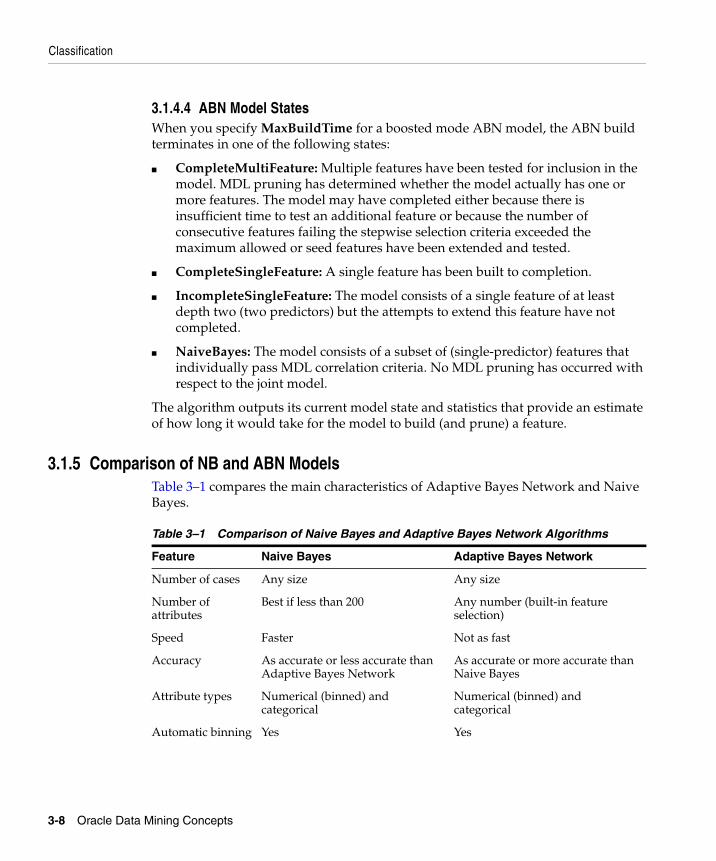
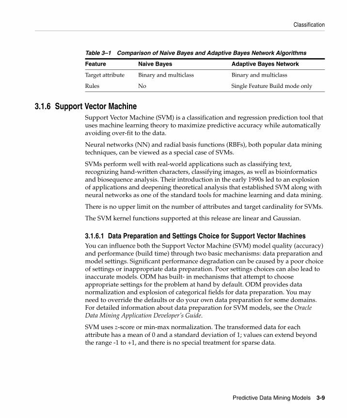
3.1.5 Comparison of NB and ABN ModelsTable 3–1 compares the main characteristics of Adaptive Bayes Network and Naive Bayes.
Table 3–1 Comparison of Naive Bayes and Adaptive Bayes Network Algorithms
Feature Naive Bayes Adaptive Bayes Network
Number of cases Any size Any size
Number of attributes
Best if less than 200 Any number (built-in feature selection)
Speed Faster Not as fast
Accuracy As accurate or less accurate than Adaptive Bayes Network
As accurate or more accurate than Naive Bayes
Attribute types Numerical (binned) and categorical
Numerical (binned) and categorical
Automatic binning Yes Yes
Classification
Predictive Data Mining Models 3-9
3.1.6 Support Vector MachineSupport Vector Machine (SVM) is a classification and regression prediction tool that uses machine learning theory to maximize predictive accuracy while automatically avoiding over-fit to the data.
Neural networks (NN) and radial basis functions (RBFs), both popular data mining techniques, can be viewed as a special case of SVMs.
SVMs perform well with real-world applications such as classifying text, recognizing hand-written characters, classifying images, as well as bioinformatics and biosequence analysis. Their introduction in the early 1990s led to an explosion of applications and deepening theoretical analysis that established SVM along with neural networks as one of the standard tools for machine learning and data mining.
There is no upper limit on the number of attributes and target cardinality for SVMs.
The SVM kernel functions supported at this release are linear and Gaussian.
3.1.6.1 Data Preparation and Settings Choice for Support Vector Machines You can influence both the Support Vector Machine (SVM) model quality (accuracy) and performance (build time) through two basic mechanisms: data preparation and model settings. Significant performance degradation can be caused by a poor choice of settings or inappropriate data preparation. Poor settings choices can also lead to inaccurate models. ODM has built- in mechanisms that attempt to choose appropriate settings for the problem at hand by default. ODM provides data normalization and explosion of categorical fields for data preparation. You may need to override the defaults or do your own data preparation for some domains. For detailed information about data preparation for SVM models, see the Oracle Data Mining Application Developer’s Guide.
SVM uses z-score or min-max normalization. The transformed data for each attribute has a mean of 0 and a standard deviation of 1; values can extend beyond the range -1 to +1, and there is no special treatment for sparse data.
Target attribute Binary and multiclass Binary and multiclass
Rules No Single Feature Build mode only
Table 3–1 Comparison of Naive Bayes and Adaptive Bayes Network Algorithms
Feature Naive Bayes Adaptive Bayes Network
Regression
3-10 Oracle Data Mining Concepts
3.2 Regression Regression creates predictive models. The difference between regression and classification is that regression deals with numerical/continuous target attributes, whereas classification deals with discrete/categorical target attributes. In other words, if the target attribute contains continuous (floating-point) values, a regression technique is required. If the target attribute contains categorical (string or discrete integer) values, a classification technique is called for.
The most common form of regression is linear regression, in which a line that best fits the data is calculated, that is, the line that minimizes the average distance of all the points from the line.
This line becomes a predictive model when the value of the dependent variable is not known; its value is predicted by the point on the line that corresponds to the values of the independent variables for that record.
3.2.1 SVM Algorithm for RegressionSupport Vector Machine (SVM) builds both classification and regression models. SVM is described in the section on classification; see Section 3.1.6, "Support Vector Machine".
3.3 Attribute ImportanceAttribute Importance (AI) provides an automated solution for improving the speed and possibly the accuracy of classification models built on data tables with a large number of attributes.
Attribute Importance ranks the predictive attributes by eliminating redundant, irrelevant, or uninformative attributes and identifying those predictor attributes that may have the most influence in making predictions. ODM examines data and constructs classification models that can be used to make predictions about subsequent data. The time required to build these models increases with the number of predictors. Attribute Importance helps a user identify a proper subset of these attributes that are most relevant to predicting the target. Model building can proceed using the selected attributes (predictor attributes) only.
Using fewer attributes decreases model building time, although sometimes at a cost in predictive accuracy. Using too many attributes (especially those that are "noise") can affect the model and degrade its performance and accuracy. By extracting as much information as possible from a given data table using the smallest number of attributes, a user can save significant computing time and often build better models.
Attribute Importance
Predictive Data Mining Models 3-11
Attribute Importance permits the user to specify a number or percentage of attributes to use; alternatively the user can specify a cutoff point. After an Attribute Importance model is built, the user can select the subset of attributes based on the ranking or the predictive value.
Attribute Importance can be applied to data tables with a very large set of attributes. However, the DBA may have to tune the database in various ways to ensure that Attribute Importance build executes efficiently. For example, it is important to ensure that there is adequate swap space and table space.
3.3.1 Minimum Descriptor LengthMinimum Description Length (MDL) is an information theoretic model selection principle. MDL assumes that the simplest, most compact representation of data is the best and most probable explanation of it.
With MDL, the model selection problem is treated as a communication problem. There is a sender, a receiver, and data to be transmitted. For classification models, the data to be transmitted is a model and the sequence of target class values in the training data. Typically, each model under consideration comes from a list of potential candidate models. The sizes of the lists vary. The models compute probabilities for the target class of each training data set row. The model's predicted probability is used to encode the training data set target values. From Shannon's noiseless coding theorem, it is known that the most compact encoding uses a number of bits equal to -log2(pi), where pi is probability of the target value in the i-th training data set row for all rows in the data set.
The sender and receiver agree on lists of potential candidate models for each model under consideration. A model in a list is represented by its position in the list (for example, model #26). The position is expressed as a binary number. Thus, for a list of length m, the number of bits in the binary number is log2(m). The sender and receiver each get a copy of the list. The sender transmits the model. Once the model is known, the sender know how to encode the targets and the receiver knows how to decode the targets. The sender then transmits the encoded targets. The total description length of a model is then:
log2(m) - Sum(log2(pi))
Note that the better the model is at estimating the target probabilities, the shorter the description length. However, the improvement in target probability estimation can come at the expense of a longer list of potential candidates. Thus the description length is a penalized likelihood of the model.
ODM Model Seeker (Java Interface Only)
3-12 Oracle Data Mining Concepts
The attribute importance problem can be put in the MDL framework, by considering each attribute as a simple predictive model of the target class. Each value of the predictor (indexed by i) has associated with it a set of ni training examples and a probability distribution, pij for the m target class values (indexed by j). From ni training examples there are at most ni pij's distinguishable in the data. From combinatorics, it is known that the number of distributions of m distinct objects in a total of n objects is n-m choose m. Hence the size of the list for a predictor is
Sumi log2((ni - m choose m))
The total description length for a predictor is then:
Sumi (log2(ni - m choose m)) - Sumij(log2(pij))
The predictor rank is the position in the list of associated description lengths, smallest first.
3.4 ODM Model Seeker (Java Interface Only)ODM Model Seeker allows a user to build multiple ABN and NB models and select the "best" model based on a predetermined criterion.
With Model Seeker, the user can compactly specify parameters for an execution that will asynchronously build and test multiple classification models. These models may be built using different algorithms. For each algorithm, Model Seeker systematically varies the algorithm parameters to create a series of parameter values that are used to create corresponding models. Model Seeker then evaluates these models and selects a "best" model using a predetermined criterion.
These features were developed to support applications that want to create a model that can be directly used in a production application environment with a minimum of user interaction. This assumes that the application developer has the expertise, or advice from someone with the expertise, to set the various algorithm parameters in a manner that is suitable to the particular business problem and data sources on which the application is to operate.
Note: Model Seeker is deprecated in Oracle Data Mining 10g Release 1 (10.1) . It will not be available in subsequent releases of ODM; the functionlaity will be supported in other ways.
ODM Model Seeker (Java Interface Only)
Predictive Data Mining Models 3-13
A secondary purpose is to present to the user or application a summary of information about each model built and tested by a Model Seeker execution so that the user or application can independently find the parameters that correspond to an alternative "best" model using a different criterion. This feature is meant to provide support for an application for use by an analyst who will experiment with alternative parameter settings to discover the appropriate settings to use in a production environment.
Model Seeker’s criterion for the "best" model is the one with the largest value for a calculated weighted relative accuracy. The weight used in this calculation is the relative importance of the positive target category to the other categories treated as a single negative category. If the weight is set to 1.0, the positive target category relative accuracy has the same weight as the relative accuracy of all the other categories combined.
The following formula is used to calculate the figure of merit (FOM) for the "best" model, where FOM is the weighted sum of the positive target relative accuracy and the total negative relative accuracy:
FOM = W * (number of correct positives) + (number of correct negatives) (W + 1) * (number of actual positives) (W + 1) * (number of actual negatives)
where W is the user-specified weight, a value that must be > 0.0. A recommended way for a user to choose a value for the weight is as follows. First, estimate the cost to the user of predictions that are all correct except for a random fixed percentage, say 5%, of positive predictions being false positives. Second, estimate the cost to the user of predictions that are all correct except for the same random fixed percentage, 5%, of negative predictions being false negatives. Use a value for weight equal to the ratio of the second estimate to the first estimate. A weight of 1.0 means that a given percentage of false negatives has the same cost as a given percentage of false positives.

ODM Model Seeker (Java Interface Only)
3-14 Oracle Data Mining Concepts
Descriptive Data Mining Models 4-1
4Descriptive Data Mining Models
This chapter describes descriptive models, that is, the unsupervised learning functions. These functions do not predict a target value, but focus more on the intrinsic structure, relations, interconnectedness, etc. of the data. The Oracle Data Mining interfaces support the following descriptive models and associated algorithms:
4.1 Clustering in Oracle Data MiningClustering is a technique useful for exploring data. It is particularly useful where there are many cases and no obvious natural groupings. Here, clustering data mining algorithms can be used to find whatever natural groupings may exist.
Clustering analysis identifies clusters embedded in the data. A cluster is a collection of data objects that are similar in some sense to one another. A good clustering method produces high-quality clusters to ensure that the inter-cluster similarity is low and the intra-cluster similarity is high; in other words, members of a cluster are more like each other than they are like members of a different cluster.
Clustering can also serve as a useful data-preprocessing step to identify homogeneous groups on which to build predictive models. Clustering models are
Function Algorithm
Clustering (Section 4.1) Enhanced k-means (Section 4.1.1)
Orthogonal Clustering (O-Cluster) Java interface only (Section 4.1.2)
Association (Section 4.2) Apriori Algorithm (Section 4.2.4)
Feature Extraction (Section 4.3)
Non-Negative Matrix Factorization (Section 4.3.1)
Clustering in Oracle Data Mining
4-2 Oracle Data Mining Concepts
different from predictive models in that the outcome of the process is not guided by a known result, that is, there is no target attribute. Predictive models predict values for a target attribute, and an error rate between the target and predicted values can be calculated to guide model building. Clustering models, on the other hand, uncover natural groupings (clusters) in the data. The model can then be used to assign groupings labels (cluster IDs) to data points.
In ODM a cluster is characterized by its centroid, attribute histograms, and place in the clustering model hierarchical tree. ODM performs hierarchical clustering using an enhanced version of the k-means algorithm and O-Cluster, an Oracle proprietary algorithm. The clusters discovered by these algorithms are then used to create rules that capture the main characteristics of the data assigned to each cluster. The rules represent the hyperboxes (bounding boxes) that envelop the data in the clusters discovered by the clustering algorithm. The antecedent of each rule describes the clustering bounding box. The consequent encodes the cluster ID for the cluster described by the rule. For example, for a data set with two attributes: AGE and HEIGHT, the following rule represents most of the data assigned to cluster 10:
If AGE >= 25 and AGE <= 40 and HEIGHT >= 5.0ft and HEIGHT <= 5.5ftthen CLUSTER = 10
The clusters are also used to generate a Bayesian probability model which is used during scoring for assigning data points to clusters.
The two clustering algorithms supported by ODM interfaces are
■ Enhanced k-means
■ Orthogonal partitioning clustering (Java interface only)
4.1.1 Enhanced k-Means AlgorithmThe k-means algorithm is a distance-based clustering algorithm that partitions the data into a predetermined number of clusters (provided there are enough distinct cases). The k-means algorithm works only with numerical attributes. Distance-based algorithms rely on a distance metric (function) to measure the similarity between data points. The distance metric is either Euclidean, Cosine, or Fast Cosine distance. (Cosine and Fast Cosine are supported in the DBMS_DATA_MINING version of k-means only.) Data points are assigned to the nearest cluster according to the distance metric used.
Clustering in Oracle Data Mining
Descriptive Data Mining Models 4-3
ODM implements an enhanced version of the k-means algorithm with the following features:
■ The algorithm builds models in a hierarchical manner. The algorithm builds a model top down using binary splits and refinement of all nodes after the children of the split node have converged. In this sense, the algorithm is similar to the bisecting k-means algorithm described in the literature. The centroid of the inner nodes in the hierarchy are updated to reflected changes as the tree evolves. The whole tree is returned.
■ The algorithm can grow the tree either one level at a time (balanced approach) or one node at a time (unbalanced approach). The node with the largest distortion (sum of distance to the node's centroid) is split to increase the size of the tree until the desired number of clusters is reached. The DBMS_DATA_MINING implementation build unbalanced trees only.
■ The Java version of the algorithm bins the build data. Binning plays the role of normalization and helps with data summarization and rules. The DBMS_DATA_MINING normalizes the data.
■ The algorithm has an internal data summarization step that allows it to scale well to data sets with large number of cases.
■ The algorithm provides probabilistic scoring/assignment of data to clusters.
■ The algorithm returns, for each cluster, a centroid (cluster prototype), histograms (one for each attribute), and a rule describing the hyperbox that encloses the majority of the data assigned to the cluster.
This incremental approach to k-means avoids the need for building multiple k-means models and provides clustering results that are consistently superior to the traditional k-means.
The k-Means Clustering algorithm implementation in DBMS_DATA_MINING is a modified and enhanced version of the implementing in the Java interface. There is no upper limit on the number of attributes and target cardinality for this implementation of k-Means. The DBMS_DATA_MINING implementation will be the ODM implementation of the k-Means Clustering algorithm in future ODM releases. Table 4–1 summarizes the differences between the two implementations.
Note: DBMS_DATA_MINING and the Java interface use different versions of the enhanced k-means algorithm. The two implementations may give different results.
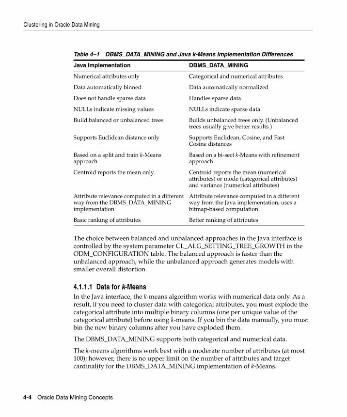
Clustering in Oracle Data Mining
4-4 Oracle Data Mining Concepts
The choice between balanced and unbalanced approaches in the Java interface is controlled by the system parameter CL_ALG_SETTING_TREE_GROWTH in the ODM_CONFIGURATION table. The balanced approach is faster than the unbalanced approach, while the unbalanced approach generates models with smaller overall distortion.
4.1.1.1 Data for k-MeansIn the Java interface, the k-means algorithm works with numerical data only. As a result, if you need to cluster data with categorical attributes, you must explode the categorical attribute into multiple binary columns (one per unique value of the categorical attribute) before using k-means. If you bin the data manually, you must bin the new binary columns after you have exploded them.
The DBMS_DATA_MINING supports both categorical and numerical data.
The k-means algorithms work best with a moderate number of attributes (at most 100); however, there is no upper limit on the number of attributes and target cardinality for the DBMS_DATA_MINING implementation of k-Means.
Table 4–1 DBMS_DATA_MINING and Java k-Means Implementation Differences
Java Implementation DBMS_DATA_MINING
Numerical attributes only Categorical and numerical attributes
Data automatically binned Data automatically normalized
Does not handle sparse data Handles sparse data
NULLs indicate missing values NULLs indicate sparse data
Build balanced or unbalanced trees Builds unbalanced trees only. (Unbalanced trees usually give better results.)
Supports Euclidean distance only Supports Euclidean, Cosine, and Fast Cosine distances
Based on a split and train k-Means approach
Based on a bi-sect k-Means with refinement approach
Centroid reports the mean only Centroid reports the mean (numerical attributes) or mode (categorical attributes) and variance (numerical attributes)
Attribute relevance computed in a different way from the DBMS_DATA_MINING implementation
Attribute relevance computed in a different way from the Java implementation; uses a bitmap-based computation
Basic ranking of attributes Better ranking of attributes
Clustering in Oracle Data Mining
Descriptive Data Mining Models 4-5
4.1.1.2 Scalability through SummarizationBecause traditional k-means requires multiple passes through the data, it can be impractical for large data tables that don’t fit in memory. In this case multiple expensive database scans would be required. ODM’s enhanced k-means requires at most one database scan. For data tables that don’t fit in memory, the enhanced k-means algorithm employs a smart summarization approach that creates a summary of the data table that can be stored in memory. This approach allows the enhanced k-means algorithm to handle data tables of any size. The summarization scheme can be seen as a smart sampling approach that first identifies the main partitions in the data and then generates summary points for each partition in proportion to their share of the total data. Each summary point has a weight that accounts for the proportion of the data it represents.
4.1.1.3 Scoring (Applying Models)The clusters discovered by enhanced k-means are used to generate a Bayesian probability model that is then used during scoring (model apply) for assigning data points to clusters. The traditional k-means algorithm can be interpreted as a mixture model where the mixture components are spherical multivariate normal distributions with the same variance for all components. A mixture model is a type of density model that includes several component functions (usually Gaussian) that are combined to provide a multimodal density.
In the mixture model created from the clusters discovered by enhanced k-means, on the other hand, the mixture components are a product of independent normal distribution with potentially different variances. Because of this greater flexibility, the probability model created by enhanced k-means provides a better description of the underlying data than the underlying model of traditional k-means.
4.1.2 Orthogonal Partitioning Clustering (O-Cluster)
The O-Cluster algorithm supports Orthogonal Partitioning Clustering; O-Cluster creates a hierarchical grid-based clustering model, that is, it creates axis-parallel (orthogonal) partitions in the input attribute space. The algorithm operates recursively. The resulting hierarchical structure represents an irregular grid that tessellates the attribute space into clusters. The resulting clusters define dense areas in the attribute space. The clusters are described by intervals along the attribute axes and the corresponding centroids and histograms. A parameter called sensitivity
Note: O-Cluster is available in the Java interface only.
Clustering in Oracle Data Mining
4-6 Oracle Data Mining Concepts
defines a baseline density level. Only areas with peak density above this baseline level can be identified as clusters.
To compare, the k-means algorithm tesselates the space even when natural clusters may not exist. For example, if there is a region of uniform density, k-Means tesselates it into n clusters (specified by the user). On the other hand, O-Cluster separates areas of high density by placing cutting planes through areas of low density. O-Cluster needs multi-modal histograms (peaks and valleys). If an area has projections with uniform or monotonically changing density, O-Cluster does not partition it.
4.1.2.1 O-Cluster Data UseO-Cluster does not necessarily use all the data when it builds a model. It reads the data in batches (the default batch size is 50000). It will only read another batch if it believes, based on some statistical tests, that there may still exist clusters that it has not uncovered.
Because O-Cluster may stop the model build before it reads all of the data, it is highly recommended that you randomize the data.
4.1.2.2 Binning for O-ClusterO-Cluster bins the data internally, thus providing automatic data discretization. However, if manual binning is used, the bin values must be represented by contiguous integer numbers starting at 1.
4.1.2.3 O-Cluster Attribute TypeBinary attributes should be declared as categorical. O-Cluster distinguishes between continuous and discrete numerical attributes. The two types of attributes undergo different binning procedures in order to capture the characteristics of the underlying distributions. For example, a discrete numerical attribute such as age should be declared of data type INTEGER. On the other hand, continuous numerical attributes such as height measured in feet should be declared of data type NUMBER.
4.1.2.4 O-Cluster ScoringThe clusters discovered by O-Cluster are used to generate a Bayesian probability model that is then used during scoring (model apply) for assigning data points to clusters. The generated probability model is a mixture model where the mixture components are represented by a product of independent normal distributions for numerical attributes and multinomial distributions for categorical attributes.
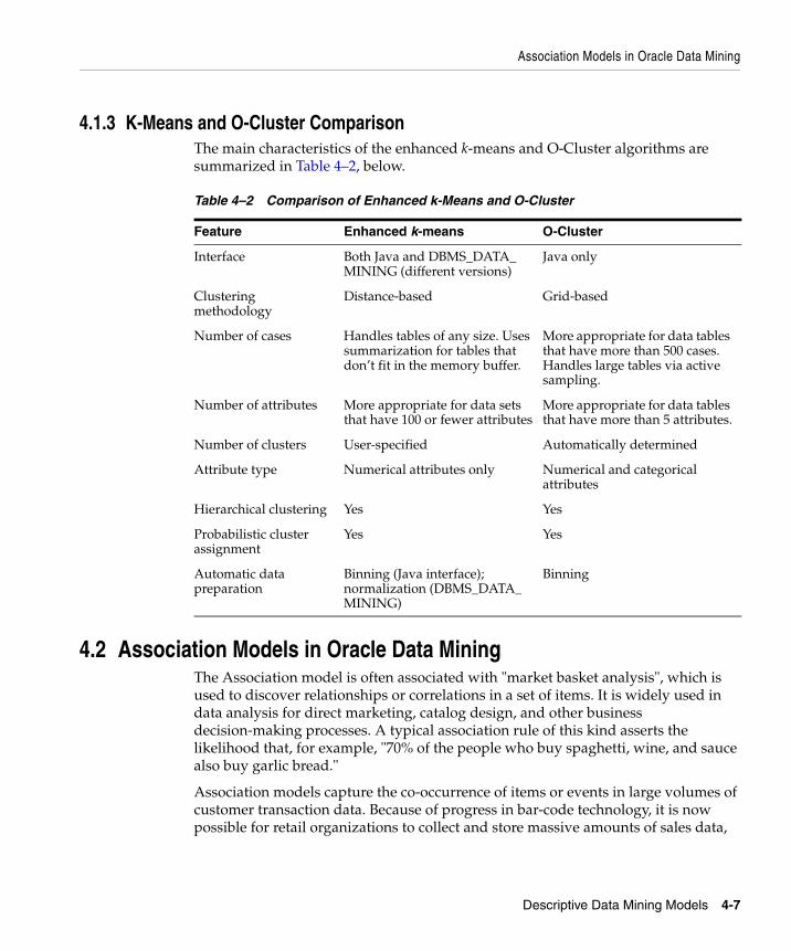
Association Models in Oracle Data Mining
Descriptive Data Mining Models 4-7
4.1.3 K-Means and O-Cluster ComparisonThe main characteristics of the enhanced k-means and O-Cluster algorithms are summarized in Table 4–2, below.
4.2 Association Models in Oracle Data MiningThe Association model is often associated with "market basket analysis", which is used to discover relationships or correlations in a set of items. It is widely used in data analysis for direct marketing, catalog design, and other business decision-making processes. A typical association rule of this kind asserts the likelihood that, for example, "70% of the people who buy spaghetti, wine, and sauce also buy garlic bread."
Association models capture the co-occurrence of items or events in large volumes of customer transaction data. Because of progress in bar-code technology, it is now possible for retail organizations to collect and store massive amounts of sales data,
Table 4–2 Comparison of Enhanced k-Means and O-Cluster
Feature Enhanced k-means O-Cluster
Interface Both Java and DBMS_DATA_MINING (different versions)
Java only
Clustering methodology
Distance-based Grid-based
Number of cases Handles tables of any size. Uses summarization for tables that don’t fit in the memory buffer.
More appropriate for data tables that have more than 500 cases. Handles large tables via active sampling.
Number of attributes More appropriate for data sets that have 100 or fewer attributes
More appropriate for data tables that have more than 5 attributes.
Number of clusters User-specified Automatically determined
Attribute type Numerical attributes only Numerical and categorical attributes
Hierarchical clustering Yes Yes
Probabilistic cluster assignment
Yes Yes
Automatic data preparation
Binning (Java interface); normalization (DBMS_DATA_MINING)
Binning
Association Models in Oracle Data Mining
4-8 Oracle Data Mining Concepts
referred to as "basket data." Association models were initially defined on basket data, even though they are applicable in several other applications. Finding all such rules is valuable for cross-marketing and mail-order promotions, but there are other applications as well: catalog design, add-on sales, store layout, customer segmentation, web page personalization, and target marketing.
Traditionally, association models are used to discover business trends by analyzing customer transactions. However, they can also be used effectively to predict Web page accesses for personalization. For example, assume that after mining the Web access log, Company X discovered an association rule "A and B implies C," with 80% confidence, where A, B, and C are Web page accesses. If a user has visited pages A and B, there is an 80% chance that he/she will visit page C in the same session. Page C may or may not have a direct link from A or B. This information can be used to create a dynamic link to page C from pages A or B so that the user can "click-through" to page C directly. This kind of information is particularly valuable for a Web server supporting an e-commerce site to link the different product pages dynamically, based on the customer interaction.
There are several properties of association models that can be calculated. ODM provides two:
■ Support: Support of a rule is a measure of how frequently the items involved in it occur together. Using probability notation, support (A implies B) = P(A, B).
■ Confidence: Confidence of a rule is the conditional probability of B given A; confidence (A implies B) = P (B given A), which is equal to P(A, B) or P(A).
These statistical measures can be used to rank the rules and hence the predictions.
ODM supports the Apriori algorithm for association models.
The Apriori algorithm works by iteratively enumerating item sets of increasing lengths subject to the minimum support threshold. Since association rule mining is defined this way and the state-of-the-art algorithms work by iterative enumeration, association rules algorithms don’t handle the following cases efficiently:
■ Finding associations involving rare events
■ Finding associations in data sets that are dense and that have a large number of attributes.
4.2.1 Finding Associations Involving Rare EventsBy definition, association rule mining discovers frequent patterns with frequency above the minimum support threshold. Therefore, in order to find associations involving rare events, the algorithm must run with very low minimum support
Association Models in Oracle Data Mining
Descriptive Data Mining Models 4-9
values. However, doing so could potentially explode the number of enumerated item sets, especially in cases with large number of items. That could increase the execution time significantly.
Therefore, association rule mining is not recommended for finding associations involving "rare" events in problem domains with large number of items.
However, there are ways to restrict the item set enumeration to a smaller set if the "rare" events of interest are known. One could also use association rules to perform "partial classification" of the rare events. Those enhancements to association rules are not supported in this release.
Another option is to use classification models in such problem domains.
4.2.2 Finding Associations in Dense Data Sets Since association rule algorithms work by iterative enumeration, they work best for sparse data sets, that is, data sets where each record contains only a small fraction of the total number of possible items (if the total number of items is very large). Algorithm performance degrades exponentially with increasing number of frequent items per record. Therefore, to get good runtime performance, one of the following conditions should hold:
■ If the data set is dense, the number of possible items is small.
■ If the number of possible items is large, the data set is sparse.
■ The data set becomes progressively sparser with increasing item set length due to the application of the minimum support threshold.
The last condition holds for higher minimum support values.
Typical data sets in many bioinformatics applications are dense with large number of attributes. In order to use association rules effectively for such problems, careful planning is required. One option is to start with a high minimum support threshold and repeat it for lower values until desirable results are obtained. Another option is to recode some of the uninteresting attribute values to NULL, if such recoding makes the data set sparse.
4.2.3 Data for Association ModelsAssociation models are designed to use sparse data. Sparse data is data for which only a small fraction of the attributes are non-zero or non-null in any given row. Examples of sparse data include market basket and text mining data. For example, a market basket problem, there might be 1,000 products in the company’s catalog,
Feature Extraction in Oracle Data Mining
4-10 Oracle Data Mining Concepts
and the average size of a basket (the collection of items that a customer purchases in a typical transaction) is 20 products. In this example, a transaction/case/record has on average 20 out of 1000 attributes that are not null. This implies that the fraction of non-zero attributes on the table (or the density) is 20/1000, or 2%. This density is typical for market basket and text processing problems. Data that has a significantly higher density can require extremely large amounts of Temp space to build associations. For more information about sparse data, see Section 2.2.6.
Association models treat NULL values an indication of sparse data. The algorithm doesn't handle missing values. If the data is not sparse and the NULL values are indeed missing at random, it is necessary to perform missing data imputation (that is, "treat" the missing values) and substitute the NULL values for a non-null value.
4.2.4 Apriori Algorithm The association rule mining problem can be decomposed into two subproblems:
■ Find all combinations of items, called frequent itemsets, whose support is greater than the minimum support.
■ Use the frequent itemsets to generate the desired rules. The idea is that if, for example, ABC and BC are frequent, then the rule A implies BC holds if the ratio of support(ABC) to support(BC) is at least as large as the minimum confidence. Note that the rule will have minimum support because ABCD is frequent. ODM Association supports single consequent rules only (ABC implies D).
The number of frequent itemsets is governed by the minimum support parameters. The number of rules generated is governed by the number of frequent itemsets and the confidence parameter. If the confidence parameter is set too high, there may be frequent itemsets in the association model but no rules.
ODM uses an SQL-based implementation of the Apriori algorithm. The candidate generation and support counting steps are implemented using SQL queries. We do not use any specialized in-memory data structures. The SQL queries are fine-tuned to run efficiently in the database server by using various hints.
4.3 Feature Extraction in Oracle Data MiningODM Feature Extraction creates a new set of features by decomposing the original data. Feature extraction lets you describe the data with a number of features far smaller than the number of original dimensions (attributes). A feature is a combination of attributes in the data that is of special interest and captures important characteristics of the data.
Feature Extraction in Oracle Data Mining
Descriptive Data Mining Models 4-11
Some applications of feature extraction are latent semantic analysis, data compression, data decomposition and projection, and pattern recognition. Feature extraction can also be used to enhance the speed and effectiveness of supervised learning.
For example, feature extraction can be used to extract the themes of a document collection, where documents are represented by a set of key words and their frequencies. Each theme (feature) is represented by a combination of keywords. The documents in the collection can then be expressed in terms of the discovered themes.
4.3.1 Non-Negative Matrix FactorizationNon-negative Matrix Factorization (NMF) is described in the paper "Learning the Parts of Objects by Non-Negative Matrix Factorization" by D. D. Lee and H. S. Seung in Nature (401, pages 788-7910, 1999). Non-negative Matrix Factorization is a feature extraction algorithm that decomposes multivariate data by creating a user-defined number of features, which results in a reduced representation of the original data. NMF decomposes a data matrix V into the product of two lower rank matrices W and H so that V is approximately equal to WH. NMF uses an iterative procedure to modify the initial values of W and H so that the product approaches V. The procedure terminates when the approximation error converges or the specified number of iterations is reached. Each feature is a linear combination of the original attribute set; the coefficients of these linear combinations are non-negative. During model apply, an NMF model maps the original data into the new set of attributes (features) discovered by the model.
There is no upper limit on the number of attributes and target cardinality for NMF.
4.3.1.1 NMF for Text MiningText mining involves extracting information from unstructured data. Further, typical text data is high-dimensional and sparse. Unsupervised algorithms like Principal Components Analysis (PCA), Singular Value Decomposition (SVD), and NMF involve factorizing the document-term matrix based on different constraints. One widely used approach for text mining is latent semantic analysis. NMF focuses on reducing dimensionality. By comparing the vectors for two adjoining segments of text in a high-dimensional semantic space, NMF provides a characterization of the degree of semantic relatedness between the segments. NMF is less complex than PCA and can be applied to sparse data. NMF-based latent semantic analysis is an attractive alternative to SVD approaches due to the additive non-negative nature of the solution and the reduced computational complexity and resource requirements.

Feature Extraction in Oracle Data Mining
4-12 Oracle Data Mining Concepts
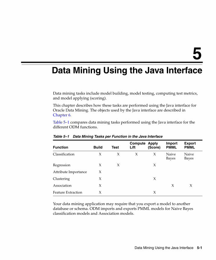
Data Mining Using the Java Interface 5-1
5Data Mining Using the Java Interface
Data mining tasks include model building, model testing, computing test metrics, and model applying (scoring).
This chapter describes how these tasks are performed using the Java interface for Oracle Data Mining. The objects used by the Java interface are described in Chapter 6.
Table 5–1 compares data mining tasks performed using the Java interface for the different ODM functions.
Your data mining application may require that you export a model to another database or schema. ODM imports and exports PMML models for Naive Bayes classification models and Association models.
Table 5–1 Data Mining Tasks per Function in the Java Interface
Function Build TestCompute Lift
Apply (Score)
Import PMML
Export PMML
Classification X X X X Naive Bayes
Naive Bayes
Regression X X X
Attribute Importance X
Clustering X X
Association X X X
Feature Extraction X X
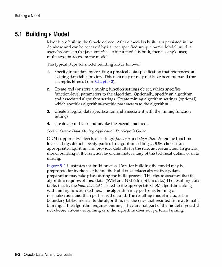
Building a Model
5-2 Oracle Data Mining Concepts
5.1 Building a ModelModels are built in the Oracle debase. After a model is built, it is persisted in the database and can be accessed by its user-specified unique name. Model build is asynchronous in the Java interface. After a model is built, there is single-user, multi-session access to the model.
The typical steps for model building are as follows:
1. Specify input data by creating a physical data specification that references an existing data table or view. This data may or may not have been prepared (for example, binned) (see Chapter 2).
2. Create and/or store a mining function settings object, which specifies function-level parameters to the algorithm. Optionally, specify an algorithm and associated algorithm settings. Create mining algorithm settings (optional), which specifies algorithm-specific parameters to the algorithm.
3. Create a logical data specification and associate it with the mining function settings.
4. Create a build task and invoke the execute method.
Seethe Oracle Data Mining Application Developer’s Guide.
ODM supports two levels of settings: function and algorithm. When the function level settings do not specify particular algorithm settings, ODM chooses an appropriate algorithm and provides defaults for the relevant parameters. In general, model building at the function level eliminates many of the technical details of data mining.
Figure 5–1 illustrates the build process. Data for building the model may be preprocess for by the user before the build takes place; alternatively, data preparation may take place during the build process. This figure assumes that the algorithm requires binned data. (SVM and NMF do not bin data.) The resulting data table, that is, the build data table, is fed to the appropriate ODM algorithm, along with mining function settings. The algorithm may performs binning or normalization, and then performs the build. The resulting model includes bin boundary tables internal to the algorithm, i.e., the ones that resulted from automatic binning, if the algorithm requires binning. They are not part of the model if you did not choose automatic binning or if the algorithm does not perform binning.
Testing a Model
Data Mining Using the Java Interface 5-3
Figure 5–1 The Build Process with Binning
5.2 Testing a ModelClassification and regression models can be tested to get an estimate of their accuracy.
After a model is built, model testing estimates the accuracy of a model’s predictions by applying the model to a new data table that has the same format as the build data table. The test results are stored in a mining test result object. A classification test result includes a confusion matrix (see Chapter 6) that allows a user to understand the type and number of classification errors made by the model.
The regression test results provide measures of model accuracy: root mean square error and mean absolute error of the prediction.
5.2.1 Computing LiftProducing a lift calculation is a way to asses a model. ODM supports computing lift for a classification model. Lift can be computed for both binary (2 values) target fields and multiclass (more than 2 values) target fields. Given a designated positive target value (that is, the value of most interest for prediction, such as "buyer," or "has disease"), test cases are sorted according to how confidently they are predicted
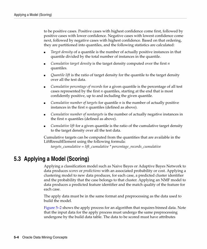
Applying a Model (Scoring)
5-4 Oracle Data Mining Concepts
to be positive cases. Positive cases with highest confidence come first, followed by positive cases with lower confidence. Negative cases with lowest confidence come next, followed by negative cases with highest confidence. Based on that ordering, they are partitioned into quantiles, and the following statistics are calculated:
■ Target density of a quantile is the number of actually positive instances in that quantile divided by the total number of instances in the quantile.
■ Cumulative target density is the target density computed over the first n quantiles.
■ Quantile lift is the ratio of target density for the quantile to the target density over all the test data.
■ Cumulative percentage of records for a given quantile is the percentage of all test cases represented by the first n quantiles, starting at the end that is most confidently positive, up to and including the given quantile.
■ Cumulative number of targets for quantile n is the number of actually positive instances in the first n quantiles (defined as above).
■ Cumulative number of nontargets is the number of actually negative instances in the first n quantiles (defined as above).
■ Cumulative lift for a given quantile is the ratio of the cumulative target density to the target density over all the test data.
Cumulative targets can be computed from the quantities that are available in the LiftRresultElement using the following formula:
targets_cumulative = lift_cumulative * percentage_records_cumulative
5.3 Applying a Model (Scoring)Applying a classification model such as Naive Bayes or Adaptive Bayes Network to data produces scores or predictions with an associated probability or cost. Applying a clustering model to new data produces, for each case, a predicted cluster identifier and the probability that the case belongs to that cluster. Applying an NMF model to data produces a predicted feature identifier and the match quality of the feature for each case.
The apply data must be in the same format and preprocessing as the data used to build the model.
Figure 5–2 shows the apply process for an algorithm that requires binned data. Note that the input data for the apply process must undergo the same preprocessing undergone by the build data table. The data to be scored must have attributes
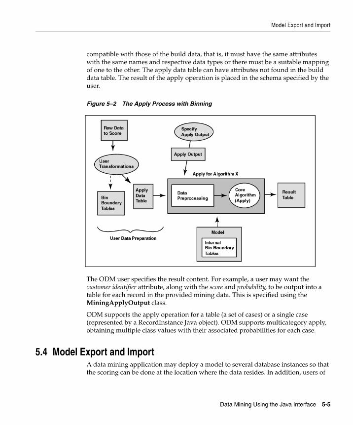
Model Export and Import
Data Mining Using the Java Interface 5-5
compatible with those of the build data, that is, it must have the same attributes with the same names and respective data types or there must be a suitable mapping of one to the other. The apply data table can have attributes not found in the build data table. The result of the apply operation is placed in the schema specified by the user.
Figure 5–2 The Apply Process with Binning
The ODM user specifies the result content. For example, a user may want the customer identifier attribute, along with the score and probability, to be output into a table for each record in the provided mining data. This is specified using the MiningApplyOutput class.
ODM supports the apply operation for a table (a set of cases) or a single case (represented by a RecordInstance Java object). ODM supports multicategory apply, obtaining multiple class values with their associated probabilities for each case.
5.4 Model Export and Import A data mining application may deploy a model to several database instances so that the scoring can be done at the location where the data resides. In addition, users of
Model Export and Import
5-6 Oracle Data Mining Concepts
different schemas may wish to share models. In both cases it is necessary to export the model from the original schema and then import it into the destination schema. Support for model export and import in the Java interface is provided by PMML.
The deployed models can score using the ODM Scoring Engine, described in.
The Predictive Model MParkup Language (PMML) specifies data mining models using an XML DTD (document type definition). PMML provides a standard representation for data mining models to facilitate model interchange among vendors. PMML is specified by the Data Mining Group (http://www.dmg.org).
The ODM Java interface is both a producer and consumer of PMML models. That is, ODM can produce (generate) a PMML model that can be used by other software that can consume PMML. ODM can also consume PMML models, that is, ODM can convert certain PMML model representations to valid ODM models. ODM is a producer and consumer of two model types: Association models and Naive Bayes classification models.
For more information about model export and import, see Chapter 9.
Objects and Functionality in the Java Interface 6-1
6Objects and Functionality in the Java
Interface
This chapter describes the principal objects in the Oracle Data Mining Java interface.
6.1 Physical Data SpecificationA physical data specification (PDS) object specifies the characteristics of the physical data to be used for mining, for example, whether the data is in multi-record case format (transactional) or single-record case (non transactional) format and the roles the various data columns play. The data referenced by a physical data specification object can be used as input to various tasks: model building, testing, computing lift, scoring, transformations, etc.
ODM physical data must be in one of two formats:■ Multi-record case (transactional)
■ Single-record case (nontransactional)
These formats describe how to interpret each case as stored in a given database table. See Chapter 2.
6.2 Mining Function SettingsA mining function settings (MFS) object contains the high-level parameters for building a mining model.
The mining function settings allow a user to specify the type of problem to solve (for example, classification) without having to specify a particular algorithm. The ODM interface allows a user to override the default algorithm. For example, if the user specifies clustering, the system may select k-means as the algorithm to build the model.
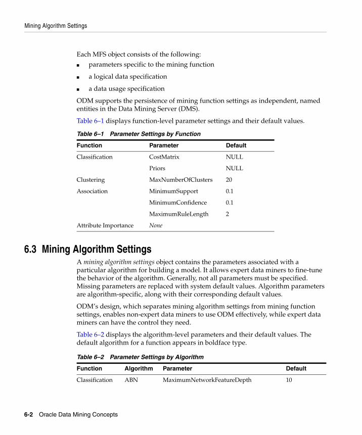
Mining Algorithm Settings
6-2 Oracle Data Mining Concepts
Each MFS object consists of the following:■ parameters specific to the mining function
■ a logical data specification
■ a data usage specification
ODM supports the persistence of mining function settings as independent, named entities in the Data Mining Server (DMS).
Table 6–1 displays function-level parameter settings and their default values.
6.3 Mining Algorithm SettingsA mining algorithm settings object contains the parameters associated with a particular algorithm for building a model. It allows expert data miners to fine-tune the behavior of the algorithm. Generally, not all parameters must be specified. Missing parameters are replaced with system default values. Algorithm parameters are algorithm-specific, along with their corresponding default values.
ODM’s design, which separates mining algorithm settings from mining function settings, enables non-expert data miners to use ODM effectively, while expert data miners can have the control they need.
Table 6–2 displays the algorithm-level parameters and their default values. The default algorithm for a function appears in boldface type.
Table 6–1 Parameter Settings by Function
Function Parameter Default
Classification CostMatrix NULL
Priors NULL
Clustering MaxNumberOfClusters 20
Association MinimumSupport 0.1
MinimumConfidence 0.1
MaximumRuleLength 2
Attribute Importance None
Table 6–2 Parameter Settings by Algorithm
Function Algorithm Parameter Default
Classification ABN MaximumNetworkFeatureDepth 10
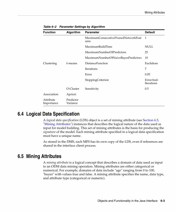
Mining Attributes
Objects and Functionality in the Java Interface 6-3
6.4 Logical Data SpecificationA logical data specification (LDS) object is a set of mining attribute (see Section 6.5, "Mining Attributes") instances that describes the logical nature of the data used as input for model building. This set of mining attributes is the basis for producing the signature of the model. Each mining attribute specified in a logical data specification must have a unique name.
As stored in the DMS, each MFS has its own copy of the LDS, even if references are shared in the interface client process.
6.5 Mining AttributesA mining attribute is a logical concept that describes a domain of data used as input to an ODM data mining operation. Mining attributes are either categorical or numerical. For example, domains of data include "age" ranging from 0 to 100, "buyer" with values true and false. A mining attribute specifies the name, data type, and attribute type (categorical or numeric).
MaximumConsecutivePrunedNetworkFeatures
1
MaximumBuildTime NULL
MaximumNumberOfPredictors 25
MaximumNumberOfNaiveBayesPredictors 10
Clustering k-means DistanceFunction Euclidean
Iterations 7
Error 0.05
StoppingCriterion ErrorAnd- Iterations
O-Cluster Sensitivity 0.5
Association Apriori
Attribute Importance
Predictor Variance
Table 6–2 Parameter Settings by Algorithm
Function Algorithm Parameter Default
Data Usage Specification
6-4 Oracle Data Mining Concepts
6.6 Data Usage SpecificationA data usage specification (DUS) object specifies how the attributes in a logical data specification (LDS) instance are used for building a model. A specification contains at most one data usage entry instance for each mining attribute in the LDS. If no data use is specified for an attribute, the default usage is active, implying that the attribute is used in building a model.
Usage includes specifying:
■ whether an attribute is active (to be used in the model build process), inactive (ignored), or supplementary (attributes that are not used for build, but for supplementary purposes such as for representing a composite attribute derived from other attributes)
■ whether an attribute is a target for a supervised learning model
6.6.1 ODM Attribute Names and CaseODM’s treatment of attribute names differs from that of Oracle SQL. Oracle SQL can treat attribute names in a case-insensitive manner; ODM attribute names, however, are case-sensitive. The implications of this for ODM users are:
■ The specification of attribute names must be consistent across build, test, compute lift, and apply tasks. For example, if a given target attribute name is specified for build in mixed-case format, then the same format must be maintained while specifying the attribute for test, apply, and lift.
■ For a MiningApply output specification, the interface allows the specification of aliases for active and supplementary attributes; the results are based on these aliases. These aliases must be unique and case-insensitive.
6.7 Mining ModelA mining model object is the result of building a model based on a mining function settings object. The representation of the model depends on the algorithm specified by the user or selected by the DMS. Some models can be used for direct inspection, for example, to examine the rules produced from association models or clusters, others to generate predictions, for example, using a classification model.
ODM supports the persistence of mining models as independent, named entities in the DMS. A mining model contains a copy of the mining function settings (MFS) used to build it. Models cannot be stored by the user.
Confusion Matrix
Objects and Functionality in the Java Interface 6-5
6.8 Mining ResultsA mining result object contains the end products of one of the following mining tasks: build, test, compute lift, or apply. ODM supports the persistence of mining results as independent, named entities in the DMS.
A mining result object contains the operation start time and end time, the name of the model used, input data location, and output data location (if any) for the data mining operation.
A build result contains the model details. It provides the function and algorithm name of the model.
An apply result names the destination table (schema and table name) for the result.
A test result, for classification models, contains the model accuracy and references the confusion matrix.
A lift result of the lift elements is calculated on a per-quantile basis.
6.9 Confusion MatrixThe row indexes of a confusion matrix correspond to actual values observed and used for model testing; the column indexes correspond to predicted values produced by applying the model to the test data. For any pair of actual/predicted indexes, the value indicates the number of records classified in that pairing. For example, a value of 25 for an actual value index of "buyer" and a predicted value index of "nonbuyer" indicates that the model incorrectly classified a "buyer" as a "nonbuyer" 25 times. A value of 516 for an actual/predicted value index of "buyer" indicates that the model correctly classified a "buyer" 516 times.
The predictions were correct 516 + 725 = 1241 times, and incorrect 25 + 10 = 35 times. The sum of the values in the matrix is equal to the number of scored records in the input data table. The number of scored records is the sum of correct and incorrect predictions, which is 1241 + 35 = 1276. The error rate is 35/1276 = 0.0274; the accuracy rate is 1241/1276 = 0.9725.
A confusion matrix provides a quick understanding of model accuracy and the types of errors the model makes when scoring records. It is the result of a test task for classification models.
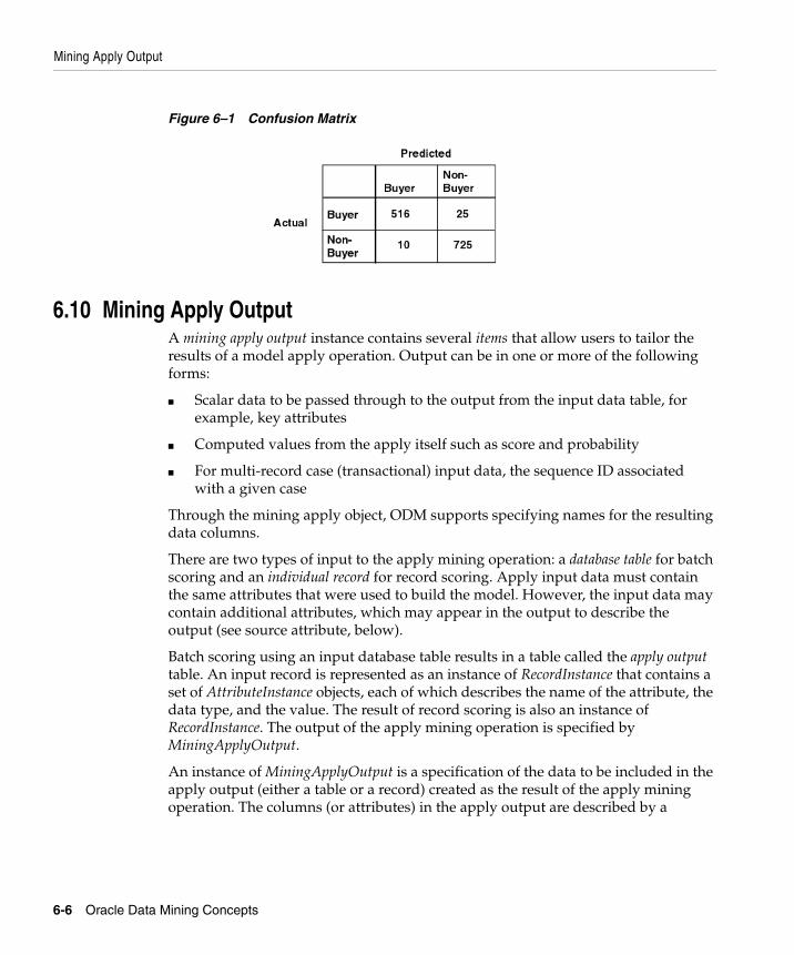
Mining Apply Output
6-6 Oracle Data Mining Concepts
Figure 6–1 Confusion Matrix
6.10 Mining Apply OutputA mining apply output instance contains several items that allow users to tailor the results of a model apply operation. Output can be in one or more of the following forms:
■ Scalar data to be passed through to the output from the input data table, for example, key attributes
■ Computed values from the apply itself such as score and probability
■ For multi-record case (transactional) input data, the sequence ID associated with a given case
Through the mining apply object, ODM supports specifying names for the resulting data columns.
There are two types of input to the apply mining operation: a database table for batch scoring and an individual record for record scoring. Apply input data must contain the same attributes that were used to build the model. However, the input data may contain additional attributes, which may appear in the output to describe the output (see source attribute, below).
Batch scoring using an input database table results in a table called the apply output table. An input record is represented as an instance of RecordInstance that contains a set of AttributeInstance objects, each of which describes the name of the attribute, the data type, and the value. The result of record scoring is also an instance of RecordInstance. The output of the apply mining operation is specified by MiningApplyOutput.
An instance of MiningApplyOutput is a specification of the data to be included in the apply output (either a table or a record) created as the result of the apply mining operation. The columns (or attributes) in the apply output are described by a
Mining Apply Output
Objects and Functionality in the Java Interface 6-7
combination of multiple ApplyContentItem objects. Each item can be one of the following:
■ Source attribute: The apply output table (or record) may contain columns copied directly from the input table (or record). These are called source attributes, and each is represented by an instance of ApplySourceAttributeItem. Source attributes can be used to identify the individual source cases in the apply output, i.e., associate a key with each output record. There can be no more than 997 source attributes in the output table.
■ Multiple predictions based on probability: An instance of ApplyMultipleScoringItem results in top or bottom n predictions ordered by probability of the predictions, where n can range from 1 to the total number of target values. One such item produces two columns in the output: prediction and probability, each of which is named by the user. There can be at most one instance of ApplyMultipleScoringItem in a MiningApplyOutput object.
Typically, users select "top" with n = 1 for obtaining the top likely prediction for each case from, for example, a classification model. However, other users may require seeing the top three predictions, for example, for recommending products to a customer.
■ Multiple predictions based on target values: An instance of ApplyTargetProbabilityItem results in predictions for target values. Each such target value must be one of the original target values used to build the model. A given target value can be specified at most once. One such item produces up to three columns in the output: prediction, probability, and rank, each of which is named by the user. Probability and rank are optional. There can be at most one instance of ApplyTargetProbabilityItem or ApplyMultipleScoringItem in a MiningApplyOutput object. This option is useful when interested in the probability of a particular prediction, for example, if a retailer has many red sweaters, what is the probability the customer would buy something red?
The number of columns in the apply output table varies depending on the combination of items. When multiple target values are specified by MiningApplyOutput (if n > 1), n rows of output table correspond to the prediction for an input row.
Consider an input table of 15 rows. If the top 2 predictions (n = 2) with probabilities are specified in MiningApplyOutput with one source attribute from the input table, there will be 3 columns in the output table: the source attribute, the prediction, and its probability.The number of rows in the output table is 30 because the result of apply for each input row will be 2 rows (top 2) in the output table.

Mining Apply Output
6-8 Oracle Data Mining Concepts
If the input data is multi-record case (transactional), the sequence ID is automatically included in the output table. However, explicit inclusion of source attributes is required for nontransactional data.
Data Mining Using DBMS_DATA_MINING 7-1
7Data Mining Using DBMS_DATA_MINING
Data mining tasks in the ODM PL/SQL interface include model building, model testing and computing lift for a model, and model applying (scoring).
The development methodology for data mining using DBMS_DATA_MINING has two phases:
■ Problem and data analysis
■ Data mining application development
7.1 DBMS_DATA_MINING Application DevelopmentAfter you’ve analyzed the problem and data, use the DBMS_DATA_MINING and DBMS_DATA_MINING_TRANSFORM packages to develop a PL/SQL application that performs the data mining:
1. Prepare the build and scoring data using the DBMS_DATA_MINING_TRANSFORM package or other third-party tool or direct SQL or PL/SQL utilities to prepare the data as required by the chosen mining function and algorithm. If you are building a predictive model, you prepare a test data set.
Note that the build, test, and score data sets must be prepared in an identical manner for mining results to be meaningful.
2. Prepare a settings table that overrides the default mining algorithm settings for the mining function and the default algorithm settings. This is also an optional step.
3. Build a mining model using the training data set.
4. For predictive models (Classification and Regression), test the model for its accuracy and other attributes. You test the model by applying it to the test data (that is, score the test data) and computing metrics on the apply results. In other
Building DBMS_DATA_MINING Models
7-2 Oracle Data Mining Concepts
words, you compare the predictions of the model with the actual values in the test data set.
5. Retrieve the model signature to determine the mining attributes required by a given model for scoring. This information helps to verify that the scoring data is suitable for scoring. This is an optional step.
6. Apply a classification, regression, clustering, or feature extraction model to new data to generate predictions or descriptive summaries and patterns about the data.
7. Retrieve the model details to understand how the model scored the data in a particular manner. This is an optional step.
8. Repeat steps 3 through 9 until you obtain satisfactory results.
7.2 Building DBMS_DATA_MINING ModelsThe DBMS_DATA_MINING package creates a mining model for a mining function using a specified mining algorithm that supports the function. The algorithm can be influenced using specific algorithm settings. Model build is synchronous in the PL/SQL interface. After a model is built, there is single-user, multi-session access to the model.
7.2.1 DBMS_DATA_MINING ModelsA model is identified by its name. Like tables in the database, a model has storage associated with it. The form, shape, and content of this storage is opaque to the user. However, the user can view the contents of a model — that is, the patterns and rules that constitute a mining model — using algorithm-specific GET_MODEL_DETAILS functions.
7.2.2 DBMS_DATA_MINING Mining FunctionsThe DBMS_DATA_MINING package supports Classification, Regression, Association, Clustering, and Feature Extraction. You specify the mining function as a parameter to the BUILD procedure.
7.2.3 DBMS_DATA_MINING Mining AlgorithmsEach mining function can be implemented using one or more algorithms. Table 7–1 provides a list of supported algorithms. There is a default algorithm for each mining
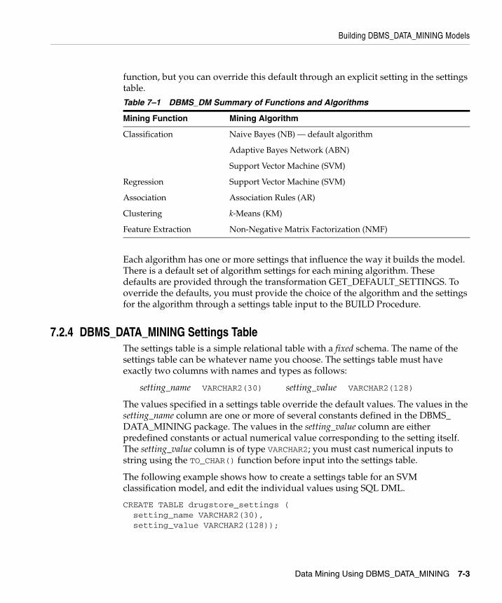
Building DBMS_DATA_MINING Models
Data Mining Using DBMS_DATA_MINING 7-3
function, but you can override this default through an explicit setting in the settings table.
Each algorithm has one or more settings that influence the way it builds the model. There is a default set of algorithm settings for each mining algorithm. These defaults are provided through the transformation GET_DEFAULT_SETTINGS. To override the defaults, you must provide the choice of the algorithm and the settings for the algorithm through a settings table input to the BUILD Procedure.
7.2.4 DBMS_DATA_MINING Settings TableThe settings table is a simple relational table with a fixed schema. The name of the settings table can be whatever name you choose. The settings table must have exactly two columns with names and types as follows:
setting_name VARCHAR2(30) setting_value VARCHAR2(128)
The values specified in a settings table override the default values. The values in the setting_name column are one or more of several constants defined in the DBMS_DATA_MINING package. The values in the setting_value column are either predefined constants or actual numerical value corresponding to the setting itself. The setting_value column is of type VARCHAR2; you must cast numerical inputs to string using the TO_CHAR() function before input into the settings table.
The following example shows how to create a settings table for an SVM classification model, and edit the individual values using SQL DML.
CREATE TABLE drugstore_settings ( setting_name VARCHAR2(30), setting_value VARCHAR2(128));
Table 7–1 DBMS_DM Summary of Functions and Algorithms
Mining Function Mining Algorithm
Classification Naive Bayes (NB) — default algorithm
Adaptive Bayes Network (ABN)
Support Vector Machine (SVM)
Regression Support Vector Machine (SVM)
Association Association Rules (AR)
Clustering k-Means (KM)
Feature Extraction Non-Negative Matrix Factorization (NMF)
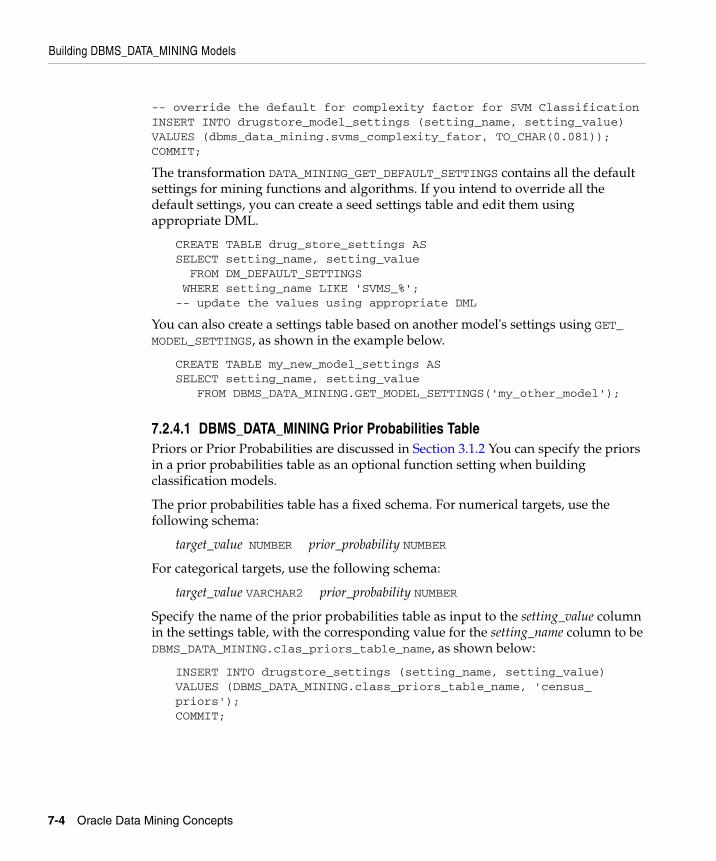
Building DBMS_DATA_MINING Models
7-4 Oracle Data Mining Concepts
-- override the default for complexity factor for SVM ClassificationINSERT INTO drugstore_model_settings (setting_name, setting_value)VALUES (dbms_data_mining.svms_complexity_fator, TO_CHAR(0.081));COMMIT;
The transformation DATA_MINING_GET_DEFAULT_SETTINGS contains all the default settings for mining functions and algorithms. If you intend to override all the default settings, you can create a seed settings table and edit them using appropriate DML.
CREATE TABLE drug_store_settings ASSELECT setting_name, setting_value FROM DM_DEFAULT_SETTINGS WHERE setting_name LIKE 'SVMS_%';-- update the values using appropriate DML
You can also create a settings table based on another model's settings using GET_MODEL_SETTINGS, as shown in the example below.
CREATE TABLE my_new_model_settings ASSELECT setting_name, setting_value
FROM DBMS_DATA_MINING.GET_MODEL_SETTINGS('my_other_model');
7.2.4.1 DBMS_DATA_MINING Prior Probabilities TablePriors or Prior Probabilities are discussed in Section 3.1.2 You can specify the priors in a prior probabilities table as an optional function setting when building classification models.
The prior probabilities table has a fixed schema. For numerical targets, use the following schema:
target_value NUMBER prior_probability NUMBER
For categorical targets, use the following schema:
target_value VARCHAR2 prior_probability NUMBER
Specify the name of the prior probabilities table as input to the setting_value column in the settings table, with the corresponding value for the setting_name column to be DBMS_DATA_MINING.clas_priors_table_name, as shown below:
INSERT INTO drugstore_settings (setting_name, setting_value) VALUES (DBMS_DATA_MINING.class_priors_table_name, 'census_priors');COMMIT;
DBMS_DATA_MINING Mining Operations and Results
Data Mining Using DBMS_DATA_MINING 7-5
7.2.4.2 DBMS_DATA_MINING Cost Matrix TableCosts are discussed in Section 3.1.1. You specify costs in a cost matrix table. The cost matrix table has a fixed schema. For numerical targets, use the following schema:
actual_target_value NUMBER predicted_target_value NUMBER cost NUMBER
For categorical targets, use the following schema:
actual_target_value VARCHAR2 predicted_target_value VARCHAR2 cost NUMBER
The DBMS_DATA_MINING package enables you to evaluate the cost of predictions from classification models in an iterative manner during the experimental phase of mining, and to eventually apply the optimal cost matrix to predictions on the actual scoring data in a production environment.
The data input to each COMPUTE procedure in the package is the result generated from applying the model on test data. If you provide a cost matrix as an input, the COMPUTE procedure generates test results taking the cost matrix into account. This enables you to experiment with various costs for a given prediction against the same APPLY results, without rebuilding the model and applying it against the same test data for every iteration.
Once you arrive at an optimal cost matrix, you can input this cost matrix to the RANK_APPLY procedure along with the results of APPLY on your scoring data. RANK_APPLY will provide your new data ranked by cost.
7.3 DBMS_DATA_MINING Mining Operations and ResultsThere are several sets of mining operations supported by the DBMS_DATA_MINING package:
■ Create, drop, and rename a model: BUILD, DROP_MODEL, RENAME_MODEL
■ Apply a model to new data: APPLY
■ Rank APPLY results or rank other data that uses the same schema as that of APPLY results: RANK_APPLY.
■ Read and describe a model: GET_MODEL_DETAILS, GET_MODEL_SETTINGS, GET_MODEL_SIGNATURE.
■ Test a classification model, based on the results of an APPLY operation on the test data, or based on any other data that uses the same schema as that of the APPLY results: COMPUTE_CONFUSION_MATRIX, COMPUTE_LIFT, and COMPUTE_ROC
DBMS_DATA_MINING Mining Operations and Results
7-6 Oracle Data Mining Concepts
■ Move a model from one schema to another or from one database instance to another: EXPORT_MODEL, IMPORT_MODEL.
The first set of operations are DDL-like operations. The last set consists of utilities. The remaining sets of operations are query-like operations in that they do not modify the model.
In addition to the operations, the following capabilities are also provided as part of the Oracle Data Mining installation:
■ User Views - DATA_MINING_USER_MODELS
■ Queries to compute metrics that test regression models.
Mining results are either returned as result sets or persisted as fixed schema tables.
7.3.1 DBMS_DATA_MINING Build ResultsThe BUILD operation creates a mining model. The GET_MODEL_DETAILS functions for each supported algorithm permit you to view the model. In addition, GET_MODEL_SIGNATURE and GET_MODEL_SETTINGS provide descriptive information about the model.
7.3.2 DBMS_DATA_MINING Apply ResultsAPPLY creates and populates a fixed schema table with a given name. The schema of this table varies based on the particular mining function, algorithm, and target attribute type — numerical or categorical.
RANK_APPLY takes an APPLY result table as input and generates another table with results ranked based on a top-N input, and for classification models, also based on cost. The schema of this table varies based on the particular mining function, algorithm, and the target attribute type — numerical or categorical.
7.3.3 Evaluating DBMS_DATA_MINING Classification ModelsDBMS_DATA_MINING includes the following procedures for testing classification models:
■ COMPUTE_CONFUSION_MATRIX — Computes the confusion matrix for a classification mo el and provides the accuracy for the model
■ COMPUTE_LIFT — Computes a lift table for a given positive target of a classification model.
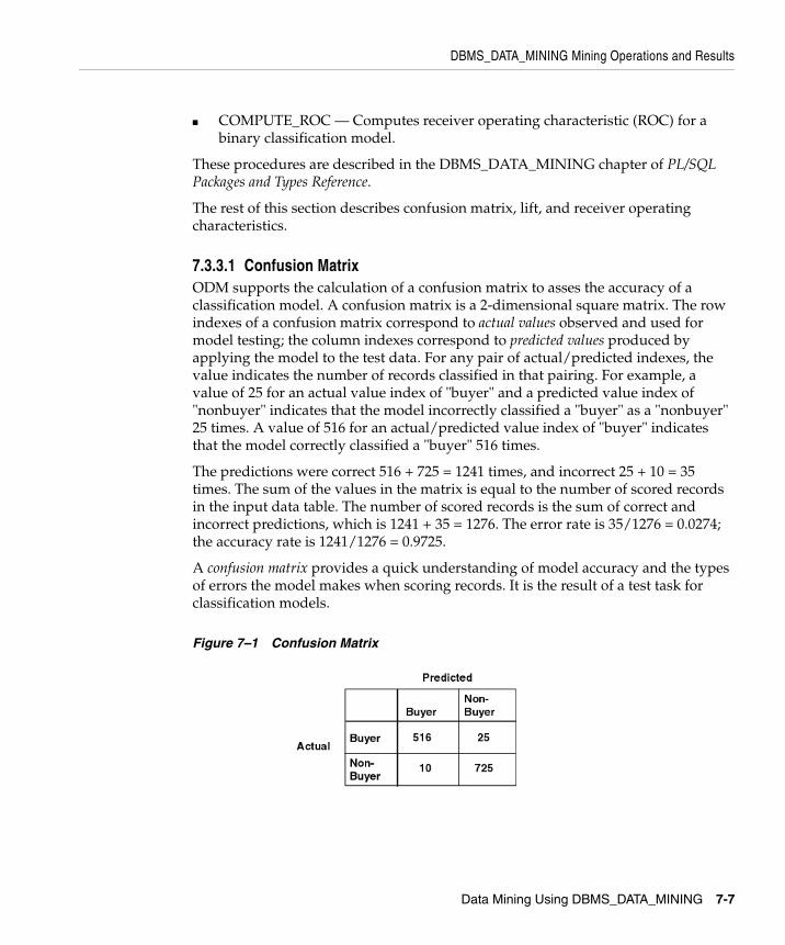
DBMS_DATA_MINING Mining Operations and Results
Data Mining Using DBMS_DATA_MINING 7-7
■ COMPUTE_ROC — Computes receiver operating characteristic (ROC) for a binary classification model.
These procedures are described in the DBMS_DATA_MINING chapter of PL/SQL Packages and Types Reference.
The rest of this section describes confusion matrix, lift, and receiver operating characteristics.
7.3.3.1 Confusion MatrixODM supports the calculation of a confusion matrix to asses the accuracy of a classification model. A confusion matrix is a 2-dimensional square matrix. The row indexes of a confusion matrix correspond to actual values observed and used for model testing; the column indexes correspond to predicted values produced by applying the model to the test data. For any pair of actual/predicted indexes, the value indicates the number of records classified in that pairing. For example, a value of 25 for an actual value index of "buyer" and a predicted value index of "nonbuyer" indicates that the model incorrectly classified a "buyer" as a "nonbuyer" 25 times. A value of 516 for an actual/predicted value index of "buyer" indicates that the model correctly classified a "buyer" 516 times.
The predictions were correct 516 + 725 = 1241 times, and incorrect 25 + 10 = 35 times. The sum of the values in the matrix is equal to the number of scored records in the input data table. The number of scored records is the sum of correct and incorrect predictions, which is 1241 + 35 = 1276. The error rate is 35/1276 = 0.0274; the accuracy rate is 1241/1276 = 0.9725.
A confusion matrix provides a quick understanding of model accuracy and the types of errors the model makes when scoring records. It is the result of a test task for classification models.
Figure 7–1 Confusion Matrix
DBMS_DATA_MINING Mining Operations and Results
7-8 Oracle Data Mining Concepts
7.3.3.2 LiftODM supports computing lift for a classification model. Lift can be computed for both binary (2 values) target fields and multiclass (more than 2 values) target fields. Given a designated positive target value (that is, the value of most interest for prediction, such as "buyer," or "has disease"), test cases are sorted according to how confidently they are predicted to be positive cases. Positive cases with highest confidence come first, followed by positive cases with lower confidence. Negative cases with lowest confidence come next, followed by negative cases with highest confidence. Based on that ordering, they are partitioned into quantiles, and the following statistics are calculated:
■ Target density of a quantile is the number of actually positive instances in that quantile divided by the total number of instances in the quantile.
■ Cumulative target density is the target density computed over the first n quantiles.
■ Quantile lift is the ratio of target density for the quantile to the target density over all the test data.
■ Cumulative percentage of records for a given quantile is the percentage of all test cases represented by the first n quantiles, starting at the end that is most confidently positive, up to and including the given quantile.
■ Cumulative number of targets for quantile n is the number of actually positive instances in the first n quantiles (defined as above).
■ Cumulative number of nontargets is the number of actually negative instances in the first n quantiles (defined as above).
■ Cumulative lift for a given quantile is the ratio of the cumulative target density to the target density over all the test data.
Cumulative targets can be computed from the quantities that are available in the LiftRresultElement using the following formula:
targets_cumulative = lift_cumulative * percentage_records_cumulative
7.3.3.3 Receiver Operating CharacteristicsAnother useful method for evaluating classification models is Receiver Operating Characteristics (ROC) analysis. ROC curves are similar to Lift charts in that they provide a means of comparison between individual models and determine thresholds which yield a high proportion of positive hits. Specifically, ROC curves aid users in selecting samples by minimizing error rates. ROC was originally used
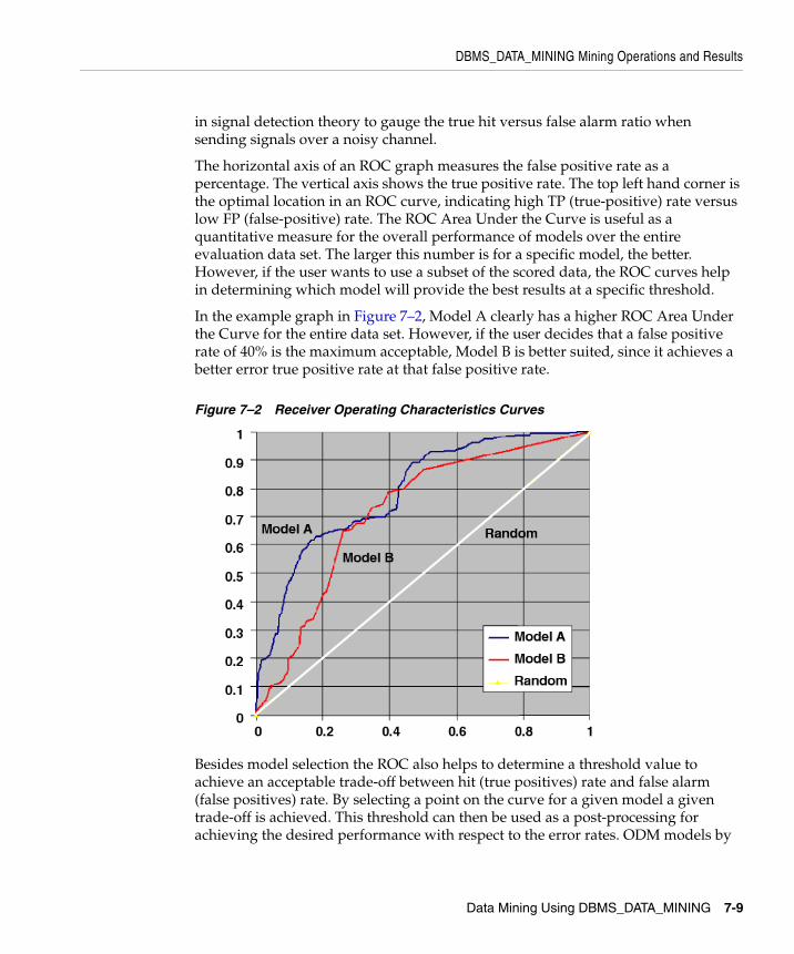
DBMS_DATA_MINING Mining Operations and Results
Data Mining Using DBMS_DATA_MINING 7-9
in signal detection theory to gauge the true hit versus false alarm ratio when sending signals over a noisy channel.
The horizontal axis of an ROC graph measures the false positive rate as a percentage. The vertical axis shows the true positive rate. The top left hand corner is the optimal location in an ROC curve, indicating high TP (true-positive) rate versus low FP (false-positive) rate. The ROC Area Under the Curve is useful as a quantitative measure for the overall performance of models over the entire evaluation data set. The larger this number is for a specific model, the better. However, if the user wants to use a subset of the scored data, the ROC curves help in determining which model will provide the best results at a specific threshold.
In the example graph in Figure 7–2, Model A clearly has a higher ROC Area Under the Curve for the entire data set. However, if the user decides that a false positive rate of 40% is the maximum acceptable, Model B is better suited, since it achieves a better error true positive rate at that false positive rate.
Figure 7–2 Receiver Operating Characteristics Curves
Besides model selection the ROC also helps to determine a threshold value to achieve an acceptable trade-off between hit (true positives) rate and false alarm (false positives) rate. By selecting a point on the curve for a given model a given trade-off is achieved. This threshold can then be used as a post-processing for achieving the desired performance with respect to the error rates. ODM models by
DBMS_DATA_MINING Mining Operations and Results
7-10 Oracle Data Mining Concepts
default use a threshold of 0.5. This is the confusion matrix reported by the test in the ODM Java interface.
The Oracle Data Mining ROC computation calculates the following statistics:
■ Probability threshold: The minimum predicted positive class probability resulting in a positive class prediction. Different threshold values result in different hit rates and false alarm rates.
■ True negatives: Negative cases in the test data with predicted probabilities below the probability threshold (correctly predicted).
■ True positives: Positive cases in the test data with predicted probabilities above the probability threshold (correctly predicted).
■ False negatives: Positive cases in the test data with predicted probabilities below the probability threshold (incorrectly predicted).
■ False positives: Negative cases in the test data with predicted probabilities above the probability threshold (incorrectly predicted).
■ Hit rate: (true positives/(true positives + false negatives))
■ False alarm rate: (false positives/(false positives + true negatives))
7.3.4 Test Results for DBMS_DATA_MINING Regression ModelsThe most commonly used metrics for regression models are root mean square error and mean absolute error. You can use SQL queries described in Oracle Data Mining Application Developer’s Guide to compute those metrics.
The regression test results provide measures of model accuracy: root mean square error and mean absolute error of the prediction.
7.3.4.1 Root Mean Square ErrorThe following query calculates root mean square.
SELECT sqrt(avg((A.prediction - B.target_column_name) * (A.prediction - B.target_column_name))) rmse FROM apply_results_table A, targets_table B WHERE A.case_id_column_name = B.case_id_column_name;
DBMS_DATA_MINING Model Export and Import
Data Mining Using DBMS_DATA_MINING 7-11
7.3.4.2 Mean Absolute ErrorGiven the targets table generated from the test data with the schema:
(case_id_column_name VARCHAR2,target_column_name NUMBER)
and apply results table for regression with the schema:
(case_id_column_name VARCHAR2, prediction NUMBER)
and a (optional) normalization table with the schema:
(attribute_name VARCHAR2(30),scale NUMBER,shift NUMBER)
the query for mean absolute error is:
SELECT /*+PARALLEL(T) PARALLEL(A)*/ AVG(ABS(T.actual_value - T.target_value)) mean_absolute_error FROM (SELECT B.case_id_column_name, (B.target_column_name * N.scale + N.shift) actual_value FROM targets_table B, normalization_table N WHERE N.attribute_name = B.target_column_name AND B.target_column_name = 1) T, apply_results_table_name A WHERE A.case_id_column_name = T.case_id_column_name;
You can fill in the italicized values with the actual column and table names chosen by you. If the data is not normalized, you can eliminate those references from the subquery.
7.4 DBMS_DATA_MINING Model Export and ImportOracle supports data mining model export and import between Oracle databases or schemas to provide a way to move models. DBMS_DATA_MINING does not support model export and import via PMML.
Model export/import is supported at different levels, as follows:
■ Database export/import. When a DBA exports a full database using the expdp utility, all the existing data mining models in the database will be exported. When a DBA imports a database dump using the impdp utility, all the data mining models in the dump will be restored.
DBMS_DATA_MINING Model Export and Import
7-12 Oracle Data Mining Concepts
■ Schema export/import. When a user or DBA exports a schema using expdp, all the data mining models in the schema will be exported. When the user or DBA imports the schema dump using impdp, all the models in the dump will be imported.
■ Selected model export/import. Users can export specified models using DBMS_DATA_MINING.export_model() and import specified models using DBMS_DATA_MINING.import_model().
DBMS_DATA_MINING supports export and import of models based on the Oracle DBMS Data Pump. Where you export a model, the tables that constitute the model and the associated metadata are written to a dump file set that consists of one or more files. When you import a model, the tables and metadata are retrieved from the file and restored in the new database.
For information about requirements for the application system, see Chapter 9.
For detailed information about the export/import transformation, see the Oracle Data Mining Application Developer’s Guide.
Text Mining Using Oracle Data Mining 8-1
8Text Mining Using Oracle Data Mining
Oracle provides support for text mining in two products:
■ Oracle Text
■ Oracle Data Mining (ODM)
The support for text data in ODM is different from that provided by Oracle Text, which is dedicated to text document processing. ODM allows the combination of text and non-text (traditional categorical and numerical) columns of data to enable clustering, classification, and feature extraction.
Support for text mining is new in ODM. Text is the first unstructured data supported by ODM. The approach ODM takes to text can also be used to integrate other unstructured data such as images, audio files, etc.
Table 8–1 summarizes how DBMS_DATA_MINING, the ODM Java interface, and Oracle Text support text mining.
Oracle Data Mining Application Developer’s Guide contains a case study that mines a combination of text data and non-text data.
8.1 What Text Mining IsText mining is conventional data mining done using "text features." Text features are usually keywords, frequencies of words, or other document-derived features. Once you derive text features, you mine them just as you would any other data.
Some of the applications for text mining include:
■ Create and manage taxonomies
■ Classify or categorize documents
ODM Technologies Supporting Text Mining
8-2 Oracle Data Mining Concepts
■ Integrating search capabilities and classification and clustering of documents returned from a search
■ Automatic extraction of topics
■ Feature extraction for subsequent mining
8.1.1 Document ClassificationDocument classification, also known as document categorization, is the process of assigning documents to categories (for example, themes or subjects). A particular document may fit into two or more different categories. This type of classification can often be represented as a multi-target classification problem where a predictive model is built for each category.
8.1.2 Combining Text and Numerical DataIn some classes of problems, text is combined with numerical data. For example patient records or other clinical records usually contain both numerical data (temperature, blood pressure, etc.) and text data (physician’s notes). In such a case, you can use ODM to perform mining on the numerical data, the text data, or both the numerical and the text data combined.
If you wish to combine both text and numerical data for mining, you must use some appropriate method to convert the unstructured data (the text) to numerical data. You convert text to numerical data by generating numbers that characterize the document. For example, you might count the number of occurrences of certain important words.
The DBMS_DATA_MINING_TRANSFORM package includes a procedure for extracting text features that gives a great deal of control on how features are treated. These features can be used in either ODM interface. The ODM Java interface, automatically converts TEXT columns, but it doesn’t provide any control over how the features are generated.
8.2 ODM Technologies Supporting Text MiningODM provides infrastructure for developing data mining applications suitable for addressing a variety of business problems involving text. Among these, the following specific technologies provide key elements for addressing problems that require text mining:
■ Classification
ODM Technologies Supporting Text Mining
Text Mining Using Oracle Data Mining 8-3
■ Clustering
■ Feature extraction
■ Association
■ Regression
The technologies that are most used in text mining are classification, clustering, and feature extraction.
8.2.1 Classification and Text MiningA large number of document classification applications fall into one of the following:
■ Assigning multiple labels to a document. ODM does not support this case.
■ Assigning a document to one of many labels. For example, automatically assigning an email message to a folder and spam filtering. This application requires supporting multi-class classification.
Support vector machines (SVMs) are powerful classifiers that have been used successfully in document classification applications. SVMs can deal with thousands of features and are easy to train with small or large amounts of data. SVMs are know to work well with text data. For more information about SVMs, see Chapter 3.
8.2.2 Clustering and Text MiningClustering is used heavily in text mining; the main applications of clustering in text mining are
■ Taxonomy generation
■ Topic extraction
■ Grouping the hits returned by a search engine
Clustering can also be used to group textual information with other indications from business databases to provide novel insights.
The current release of ODM adds support for clustering text features using the DBMS_DATA_MINING package.
Oracle Support for Text Mining
8-4 Oracle Data Mining Concepts
8.2.3 Feature Extraction and Text MiningThere are two kinds of problems for which feature extraction is useful:
■ Extract features from actual text. Oracle Text is designed to solve this kind of problem. DBMS_DATA_MINING also supports feature extraction from text. Most text mining is focused on this problem.
■ Extract semantic features or higher-level features from the basic features uncovered when features are extracted from actual text. Statistical techniques, such as single value decomposition (SVD) and non-negative matrix factorization (NMF), are important in solving this kind of problem. Higher-order features can greatly improve the quality of information retrieval, classification, and clustering tasks.
Non-negative matrix factorization (NMF) is a new feature in release 10.1 of ODM. NMF has been found to provide superior text retrieval when compared to SVD and other traditional decomposition methods. NMF takes as input a term-document matrix and generates a set of topics that represent weighted sets of co-occurring terms. The discovered topics form a basis that provides an efficient representation of the original documents. For more information about NMF, see Chapter 4, "Descriptive Data Mining Models"or Chapter 4, "Descriptive Data Mining Models".
8.2.4 Association and Regression and Text MiningAssociation models can be used to uncover the semantic meaning of words. For example, suppose that the word sheep co-occurs with words like sleep, fence, chew, grass, meadow, farmer, and shear. An association model would include rules connecting sheep with these concepts. Inspection of the rules would provide context for sheep in the document collection. Such associations can improve information retrieval engines.
Regression is most often used in problems that combine text with other types of data.
8.3 Oracle Support for Text MiningTable 8–1 summarizes how the ODM Java interface, DBMS_DATA_MINING (the ODM PL/SQL package), and Oracle Text support text mining functions.
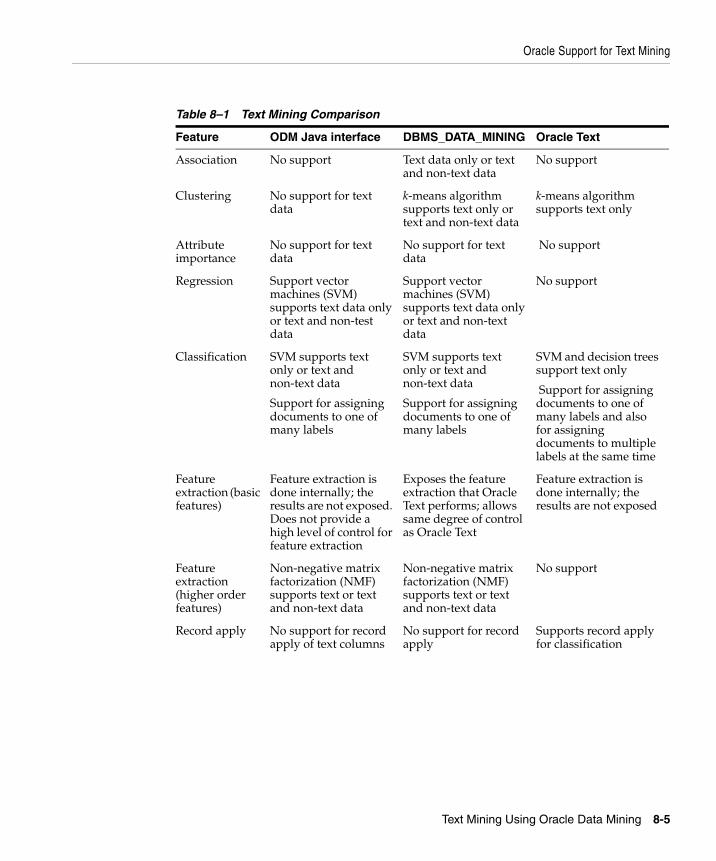
Oracle Support for Text Mining
Text Mining Using Oracle Data Mining 8-5
Table 8–1 Text Mining Comparison
Feature ODM Java interface DBMS_DATA_MINING Oracle Text
Association No support Text data only or text and non-text data
No support
Clustering No support for text data
k-means algorithm supports text only or text and non-text data
k-means algorithm supports text only
Attribute importance
No support for text data
No support for text data
No support
Regression Support vector machines (SVM) supports text data only or text and non-test data
Support vector machines (SVM) supports text data only or text and non-text data
No support
Classification SVM supports text only or text and non-text data
Support for assigning documents to one of many labels
SVM supports text only or text and non-text data
Support for assigning documents to one of many labels
SVM and decision trees support text only
Support for assigning documents to one of many labels and also for assigning documents to multiple labels at the same time
Feature extraction (basic features)
Feature extraction is done internally; the results are not exposed. Does not provide a high level of control for feature extraction
Exposes the feature extraction that Oracle Text performs; allows same degree of control as Oracle Text
Feature extraction is done internally; the results are not exposed
Feature extraction (higher order features)
Non-negative matrix factorization (NMF) supports text or text and non-text data
Non-negative matrix factorization (NMF) supports text or text and non-text data
No support
Record apply No support for record apply of text columns
No support for record apply
Supports record apply for classification
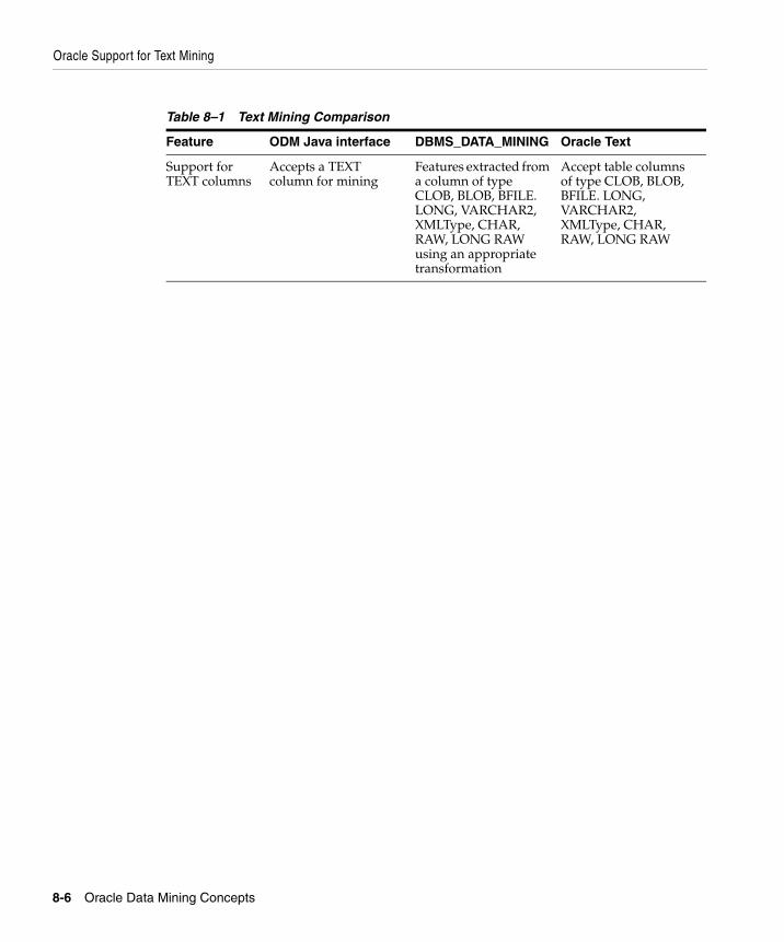
Oracle Support for Text Mining
8-6 Oracle Data Mining Concepts
Support for TEXT columns
Accepts a TEXT column for mining
Features extracted from a column of type CLOB, BLOB, BFILE. LONG, VARCHAR2, XMLType, CHAR, RAW, LONG RAW using an appropriate transformation
Accept table columns of type CLOB, BLOB, BFILE. LONG, VARCHAR2, XMLType, CHAR, RAW, LONG RAW
Table 8–1 Text Mining Comparison
Feature ODM Java interface DBMS_DATA_MINING Oracle Text
Oracle Data Mining Scoring Engine 9-1
9Oracle Data Mining Scoring Engine
Some data-mining enabled applications have models that are developed on one system and then deployed to other (production) systems. Production applications often need only to apply models built elsewhere. The Oracle Data Mining Scoring Engine supports scoring data (applying models) using models created elsewhere.
The Scoring Engine allows customers to limit the Oracle Data Mining (ODM) functionality available within their scoring applications to ensure that compute-intensive operations such as model building are not performed on systems where Scoring Engine is installed.
9.1 Oracle Data Mining Scoring Engine FeaturesThe ODM Scoring Engine supports operations for preparing data as required from the build process, importing a model, and applying a model to data. All transformation functionality is included in the Scoring Engine. All functionality provided in the Scoring Engine behaves exactly as the full system.
You cannot build models using the Scoring Engine.
9.2 Data Mining Scoring Engine Installation“Data Mining Scoring Engine” is a custom install option for Oracle Data Mining; select this option to install the ODM Scoring Engine.
9.3 Scoring in Data Mining ApplicationsA single model can be used to score large volumes of data, often in multiple geographically distributed application settings. Data analysis and model building might be performed by a small group of data mining experts using data from a
Moving Data Mining Models
9-2 Oracle Data Mining Concepts
centralized data warehouse. However, the model, can be used by a much larger number of applications working with data at geographically dispersed sites using local data. Local data may consist of millions of records representing customers; therefore, it can make sense to move the model to where the data is.
In real-time applications such as call centers, models are often built in one environment and used in another. There may be one machine dedicated to model building, using large volumes of data to produce models on a daily basis. Several other machines may be dedicated to real-time scoring, receiving new models to support, for example, the call center application. Call center representatives collect information from callers; the collected information is then used to obtain predictions or recommendations for that particular caller in real time. Scoring in real time often requires that the model is moved to where the data is.
9.4 Moving Data Mining ModelsOracle Data Mining supports two ways to move models from one schema or debase instance to another:
■ PMML export and import in the Java interface
■ Native export and import in the PL/SQL interface
9.4.1 PMML Export and ImportYou can transport Naive Bayes and Association models between ODM instances using the Export task followed by the Import to import. The PMML string produced by the Export task can be moved via file transport mechanisms for import at a target ODM instance or Scoring Engine instance. The ODM Export Task places the PMML string in a table in a cell of type CLOB, The Import Task reads the PMML string from a table cell of type CLOB. The sample program PMMLDemo.java illustrates exporting and importing a Naive Bayes model.
9.4.2 Native ODM Export and ImportIn a narrow sense, native export and import implies moving data mining model out of and into Oracle databases using Oracle proprietary facilities.
Native export and import are currently supported for data mining models built using the ODM PL/SQL interface only, namely those models created using the DBMS_DATA_MINING package.
Naive model export and import is based on Oracle Data Pump technology.
Using the Oracle Data Mining Scoring Engine
Oracle Data Mining Scoring Engine 9-3
Native export is supported at three different levels, as follows:
■ When a full database is exported using the Oracle Data Pump Export Utility (expdp), all data mining models in the database are exported.
■ When a schema is exported using the Oracle Data Pump Export Utility (expdp), all data mining models in the schema are exported.
■ An ODM user can export one or more specific models in a schema using the DBMS_DATA_MINING.export_model procedure.
Native import is also supported in all scenarios. Using the dump file set produced by the Oracle Data Pump Export Utility (expdp), an ODM user can run the Oracle Data Pump Import Utility (impdp) to import all data mining models contained in the dump file set.
ODM users can import a specific model from the dump file set using DBMS_DATA_MINING.import_model procedure.
For more information about native export and import, see the Oracle Data Mining Administrator's Guide and the DBMS_DATA_MINING chapter in the PL/SQL Packages and Types Reference.
9.5 Using the Oracle Data Mining Scoring EngineSuppose that the application builds a model on one system named BLDSYS and applies the model on a different system named SCORESYS.
BLDYS must have ODM installed. ODM supports all data mining activities (building models, testing models, applying models, etc.). SCORESYS can have the ODM Scoring Engine installed. It will not be possible to build models on SCORESYS, but it will be possible to apply the model. Note that SCORESYS could have a full ODM product installation.
The following processing takes place:
1. Build models on BLDYSYS. Select the appropriate model to deploy.
2. Export the model using the ODM PL/SQL interface (or use the Java interface to export Naive Bayes and Association models).
3. Copy the dump file generated by model export to SCORESYS. If you used PMML export, copy the PMML XML string to SCORESYS and export the string from the table cell.
4. Import the model on SCORESYS using the corresponding interface that you used to export it.

Using the Oracle Data Mining Scoring Engine
9-4 Oracle Data Mining Concepts
5. Apply the model to data on SCORESYS.
Sequence Similarity Search and Alignment (BLAST) 10-1
10 Sequence Similarity Search and Alignment
(BLAST)
In addition to data mining functions that produce predictive and descriptive models, ODM supports specialized sequence search and alignment algorithms (BLAST). In life sciences, vast quantities of data including nucleotide and amino acid sequences are stored, typically in a database. These sequence data help biologists determine the chemical structure, biological function, and evolutionary history of organisms. A key feature of managing the exponential growth in sequence data sources is the availability of fast, sensitive, and statistically rigorous techniques for detecting similarities between these sequences.
As the amount of nucleotide and amino acid sequence data continues to grow, the data becomes increasingly useful in the analysis of newly sequenced genes and proteins because of the greater chance of finding such sequence similarities.
10.1 Bioinformatics Sequence Search and AlignmentSequence alignment is one of the most commonly used bioinformatics tasks. It is present in almost any research and development activity across the many industries in the area of life sciences including academia, biotech, services, software, pharma, and hospitals.
Of all the sequence alignment algorithms, the one that is most widely used is BLAST (basic local alignment search tool). It is typically used to compare one query nucleotide or protein sequence against a database of sequences, and uncover similarities and sequence matches. Its success and popularity comes from its combination of speed, sensitivity, and statistical assessment of the results.
BLAST is a heuristic method to find the high-scoring locally optimal alignments between a query sequence and a database. The BLAST algorithm and family of
BLAST in the Oracle Database
10-2 Oracle Data Mining Concepts
programs rely on the statistics of gapped and un-gapped sequence alignments. The statistics allow the probability of obtaining an alignment with a particular score to be estimated. BLAST is unlikely to be as sensitive for all protein searches as a full dynamic programming algorithm. However, the underlying statistics provide a direct estimate of the significance of any match found.
The inclusion of BLAST in ODM positions the Oracle DBMS as a platform for bioinformatics.
10.2 BLAST in the Oracle DatabaseImplementing BLAST in the database provides the following benefits:
■ You can include BLAST in complex queries, thereby enabling complex analytical pipelines that include BLAST searches.
■ You can subselect portions of the database using SQL, thereby restricting searches.
■ Since sequence data is already stored in the database, it is not necessary to export the sequence data and pre-process them to create BLAST data sets and then import the results back into the database.
10.3 Oracle Data Mining Sequence Search and Alignment CapabilitiesSequence search and alignment, with capabilities similar to those of NCBI BLAST 2.0, has been implemented in the database using table functions. This implementation enables users to perform queries against data that is held directly inside an Oracle database. As the algorithms are implemented as table functions, parallel computation is intrinsically supported.
The five core variants of BLAST have been implemented:
■ BLASTN compares a nucleotide query sequence against a nucleotide database.
■ BLASTP compares a protein query sequence against a protein sequence database.
■ BLASTX compares the six-frame conceptual translation products of a nucleotide query sequence (both strands) against a protein sequence database.
■ TBLASTN compares a protein query sequence against a nucleotide sequence database dynamically translated in all six reading frames (both strands).
■ TBLASTX compares the six-frame translations of a nucleotide query sequence against the six-frame translations of a nucleotide sequence database.
Oracle Data Mining Sequence Search and Alignment Capabilities
Sequence Similarity Search and Alignment (BLAST) 10-3
The BLAST table functions are implemented in the database, and can be invoked by SQL. Using SQL, it is possible to pre-process the sequences as well as perform any required post-processing. This additional processing capability means it is possible to combine BLAST searches with queries that involve images, date functions, literature search, etc. Using these complex queries make it possible to perform BLAST searches on a required subset of data, potentially resulting in highly performant queries. This functionality is expected to provide considerable value.
BLAST queries can be invoked directly using the SQL interface or through an application. The query below shows an example of a SQL-invoked BLAST search where a protein sequence is compared with the protein database SwissProt, and sequences are filtered so that only human sequences that were deposited after 1 January 1990 are searched against. The column of numbers at the end of the query reflects the parameters chosen.
select t_seq_id, alignment_length, q_seq_start, q_seq_end q_frame, t_seq_start, t_seq_end, t_frame, score, expect from TABLE( BLASTP_ALIGN ( (select sequence from query_db), CURSOR(SELECT seq_id, seq_data FROM swissprot WHERE organism = 'Homo sapiens (Human)' AND creation_date > '01-Jan-90'), 1, -1, 0, 0, 'BLOSUM62', 10, 0, 0, 0, 0, 0) );
The results of a SQL query can be displayed either through an application or a SQL*Plus interface. When the SQL*Plus interface is used, the user can decide how the results will be displayed. The following shows an example of the format of the output that could be displayed by the SQL query shown above.
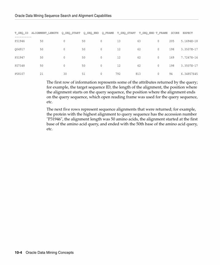
Oracle Data Mining Sequence Search and Alignment Capabilities
10-4 Oracle Data Mining Concepts
T_SEQ_ID ALIGNMENT_LENGTH Q_SEQ_START Q_SEQ_END Q_FRAME T_SEQ_START T_SEQ_END T_FRAME SCORE EXPECT----------P31946 50 0 50 0 13 63 0 205 5.1694E-18
Q04917 50 0 50 0 12 62 0 198 3.3507E-17
P31947 50 0 50 0 12 62 0 169 7.7247E-14
P27348 50 0 50 0 12 62 0 198 3.3507E-17
P58107 21 30 51 0 792 813 0 94 6.34857645
The first row of information represents some of the attributes returned by the query; for example, the target sequence ID, the length of the alignment, the position where the alignment starts on the query sequence, the position where the alignment ends on the query sequence, which open reading frame was used for the query sequence, etc.
The next five rows represent sequence alignments that were returned; for example, the protein with the highest alignment to query sequence has the accession number "P31946", the alignment length was 50 amino acids, the alignment started at the first base of the amino acid query, and ended with the 50th base of the amino acid query, etc.
ODM Interface Comparison A-1
AODM Interface Comparison
The Java and PL/SQL interfaces for Oracle Data Mining (ODM) provide similar functionality; however, they are not identical. They are aimed at different audiences; they support different features on a detailed level; and they must be used differently in different programming environments. This appendix compares the two interfaces.
A.1 Target Users of the ODM InterfacesThe two interfaces are aimed at different audiences, as follows:
■ The ODM Java interface is designed to support the development of interactive and batch mining applications and tools. The ODM Java interface is a complete interface for general-purpose application development. All mining operations, such as model build, apply, test, and lift, are executed as asynchronous tasks. The interface also supports wrapper operations -- which may involve one or more iterations of the core operations -- such as Model Seeker and utilities like import and export of PMML models. The interface also provides internal packages to support Data Mining for Java (DM4J).
■ The PL/SQL interface is designed to support traditional Oracle RDBMS application developers and DBAs who are familiar with SQL and PL/SQL packages. The DBMS_DATA_MINING package provides a set of core data mining primitives that enable creation, drop, or rename of a data mining model, and scoring of new data using a given model. The package also contains a set of helper functions for evaluating a model and for inspecting the contents of a model. All operations are synchronous. Data is not preprocessed implicitly by any of the operations. DBMS_DATA_MINING_TRANSFORM, a complementary, open-sourced package, provides a set of utilities to preprocess the data to be used for model creation, model testing, and for scoring new data using an existing model.
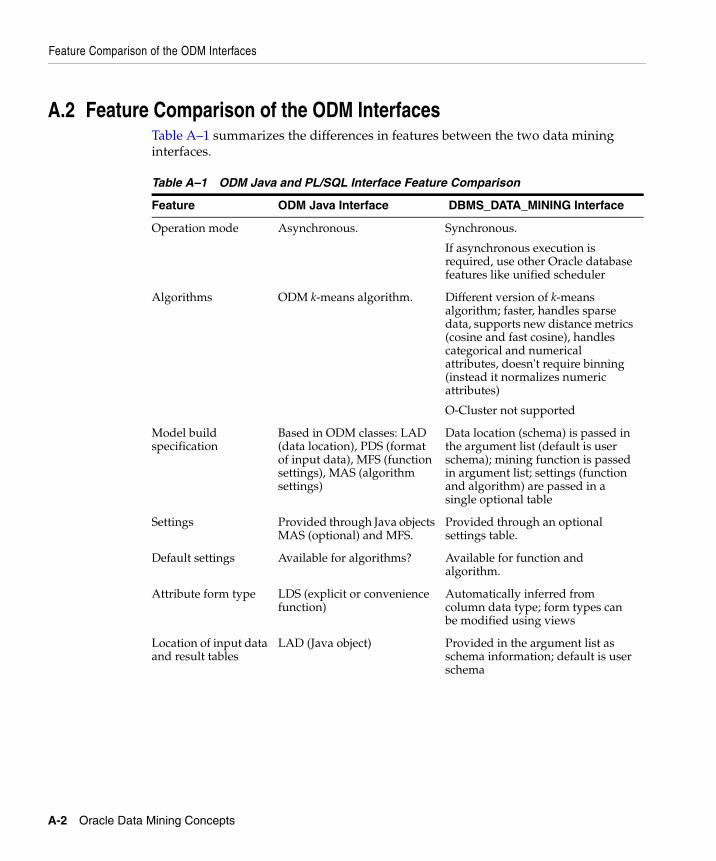
Feature Comparison of the ODM Interfaces
A-2 Oracle Data Mining Concepts
A.2 Feature Comparison of the ODM InterfacesTable A–1 summarizes the differences in features between the two data mining interfaces.
Table A–1 ODM Java and PL/SQL Interface Feature Comparison
Feature ODM Java Interface DBMS_DATA_MINING Interface
Operation mode Asynchronous. Synchronous.
If asynchronous execution is required, use other Oracle database features like unified scheduler
Algorithms ODM k-means algorithm. Different version of k-means algorithm; faster, handles sparse data, supports new distance metrics (cosine and fast cosine), handles categorical and numerical attributes, doesn't require binning (instead it normalizes numeric attributes)
O-Cluster not supported
Model build specification
Based in ODM classes: LAD (data location), PDS (format of input data), MFS (function settings), MAS (algorithm settings)
Data location (schema) is passed in the argument list (default is user schema); mining function is passed in argument list; settings (function and algorithm) are passed in a single optional table
Settings Provided through Java objects MAS (optional) and MFS.
Provided through an optional settings table.
Default settings Available for algorithms? Available for function and algorithm.
Attribute form type LDS (explicit or convenience function)
Automatically inferred from column data type; form types can be modified using views
Location of input data and result tables
LAD (Java object) Provided in the argument list as schema information; default is user schema
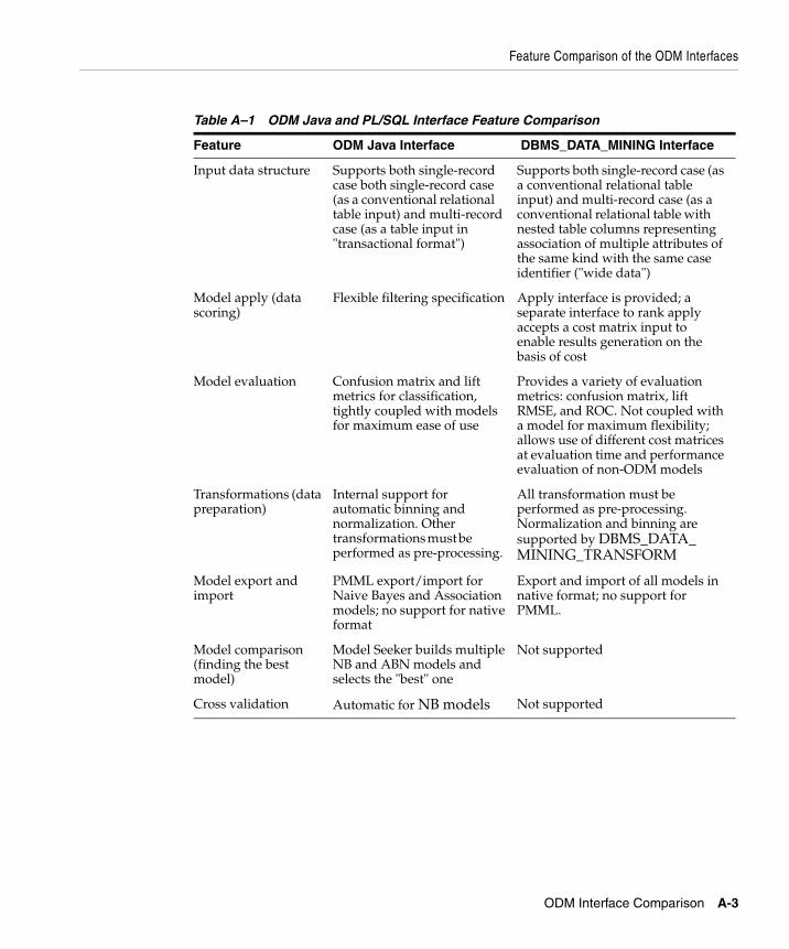
Feature Comparison of the ODM Interfaces
ODM Interface Comparison A-3
Input data structure Supports both single-record case both single-record case (as a conventional relational table input) and multi-record case (as a table input in "transactional format")
Supports both single-record case (as a conventional relational table input) and multi-record case (as a conventional relational table with nested table columns representing association of multiple attributes of the same kind with the same case identifier ("wide data")
Model apply (data scoring)
Flexible filtering specification Apply interface is provided; a separate interface to rank apply accepts a cost matrix input to enable results generation on the basis of cost
Model evaluation Confusion matrix and lift metrics for classification, tightly coupled with models for maximum ease of use
Provides a variety of evaluation metrics: confusion matrix, lift RMSE, and ROC. Not coupled with a model for maximum flexibility; allows use of different cost matrices at evaluation time and performance evaluation of non-ODM models
Transformations (data preparation)
Internal support for automatic binning and normalization. Other transformations must be performed as pre-processing.
All transformation must be performed as pre-processing. Normalization and binning are supported by DBMS_DATA_MINING_TRANSFORM
Model export and import
PMML export/import for Naive Bayes and Association models; no support for native format
Export and import of all models in native format; no support for PMML.
Model comparison (finding the best model)
Model Seeker builds multiple NB and ABN models and selects the "best" one
Not supported
Cross validation Automatic for NB models Not supported
Table A–1 ODM Java and PL/SQL Interface Feature Comparison
Feature ODM Java Interface DBMS_DATA_MINING Interface
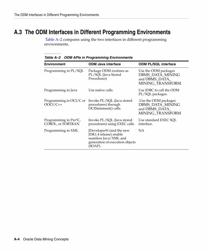
The ODM Interfaces in Different Programming Environments
A-4 Oracle Data Mining Concepts
A.3 The ODM Interfaces in Different Programming Environments Table A–2 compares using the two interfaces in different programming environments.
Programming in XML programming in PL/SQL
Table A–2 ODM APIs in Programming Environments
Environment ODM Java interface ODM PL/SQL interface
Programming in PL/SQL Package ODM routines as PL/SQL (Java Stored Procedures)
Use the ODM packages DBMS_DATA_MINING and DBMS_DATA_MINING_TRANSFORM.
Programming in Java Use native calls. Use JDBC to call the ODM PL/SQL packages.
Programming in OCI/C or OOCI/C++
Invoke PL/SQL (Java stored procedures) through OCIStatement() calls.
.Use the ODM packages DBMS_DATA_MINING and DBMS_DATA_MINING_TRANSFORM
Programming in Pro*C, COBOL, or FORTRAN
Invoke PL/SQL (Java stored procedures) using EXEC calls
Use standard EXEC SQL interface.
Programming in XML JDeveloper9i (and the new JDK1.4 release) enable seamless Java/XML and generation of execution objects (SOAP).
NA
Glossary-1
Glossary
ABN
See adaptive bayes network.
adaptive bayes network
An Oracle proprietary algorithm that can generate "rules". ABN provides a fast, scalable, non-parametric means of extracting predictive information from data with respect to a target attribute.
algorithm
A specific technique or procedure for producing a data mining model. An algorithm uses a specific model representation and may support one or more functional areas. Examples of algorithms used by ODM include Naive Bayes, Adaptive Bayes Networks, and Support Vector Machine for classification, Support Vector Machine for regression, k-means and O-Cluster for clustering, MDL for attribute importance, and Apriori for association models.
algorithm settings
The settings that specify algorithm-specific behavior for model building.
apply output
A user specification in the ODM Java interface describing the kind of output desired from applying a model to data. This output may include predicted values, associated probabilities, key values, and other supplementary data.
approximation
See regression.
Glossary-2
association
A data mining function that captures co-occurrence of items among transactions. A typical rule is an implication of the form A -> B, which means that the presence of itemset A implies the presence of itemset B with certain support and confidence. The support of the rule is the ratio of the number of transactions where the itemsets A and B are present to the total number of transactions. The confidence of the rule is the ratio of the number of transactions where the itemsets A and B are present to the number of transactions where itemset A is present. ODM uses the Apriori algorithm for association models.
association rules
Generated by association models. See association.
attribute
In the Java interface, an instance of Attribute maps to a column with a name and data type. The attribute corresponds to a column in a database table. When assigned to a column, the column must have a compatible data type; if the data type is not compatible, a runtime exception is likely. Attributes are also called variables, features, data fields, or table columns.
attribute importance
A measure of the importance of an attribute in predicting a specified target. The measure of different attributes of a build data table enables users to select the attributes that are found to be most relevant to a mining model. A smaller set of attributes results in a faster model build; the resulting model could be more accurate. ODM uses the minimum description length principle to discover important attributes. Sometimes referred to as feature selection and key fields.
attribute usage
Specifies how a logical attribute is to be used when building a model, for example, active or supplementary, suppressing automatic data preprocessing, and assigning a weight to a particular attribute. See also attributes usage set.
attributes usage set
A collection of attribute usage objects that together determine how the logical attributes specified in a logical data object are to be used.
binning
See discretization.
Glossary-3
case
All the data collected about a specific transaction or related set of values.
categorical attribute
An attribute where the values correspond to discrete categories. For example, state is a categorical attribute with discrete values (CA, NY, MA, etc.). Categorical attributes are either non-ordered (nominal) like state, gender, etc., or ordered (ordinal) such as high, medium, or low temperatures.
category
In the Java interface, corresponds to a distinct value of a categorical attribute. Categories may have string or numeric values. String values must not exceed 64 characters in length.
centroid
See cluster centroid.
classification
A data mining function for predicting categorical target values for new records using a model built from records with known target values. ODM supports three algorithms for classification, Naive Bayes, Adaptive Bayes Networks, and Support Vector Machines.
cluster centroid
The cluster centroid is the vector that encodes, for each attribute, either the mean (if the attribute is numerical) or the mode (if the attribute is categorical) of the cases in the build data assigned to a cluster.
clustering
A data mining function for finding naturally occurring groupings in data. More precisely, given a set of data points, each having a set of attributes, and a similarity measure among them, clustering is the process of grouping the data points into different clusters such that data points in the same cluster are more similar to one another and data points in different clusters are less similar to one another. ODM supports two algorithms for clustering, k-means and orthogonal partitioning clustering.
confusion matrix
Measures the correctness of predictions made by a model from a test task. The row indexes of a confusion matrix correspond to actual values observed and provided in
Glossary-4
the test data. These were used for model building. The column indexes correspond to predicted values produced by applying the model to the test data. For any pair of actual/predicted indexes, the value indicates the number of records classified in that pairing.
When predicted value equals actual value, the model produces correct predictions. All other entries indicate errors.
cost matrix
A two-dimensional, n by n table that defines the cost associated with a prediction versus the actual value. A cost matrix is typically used in classification models, where n is the number of distinct values in the target, and the columns and rows are labeled with target values. The rows are the actual values; the columns are the predicted values.
cross-validation
A technique for evaluating the accuracy of a classification or regression model. This technique is used when there are insufficient cases for using separate sets of data for model building and testing. The data table is divided into several parts, with each part in turn being used to evaluate a model built using the remaining parts. Cross-validation occurs automatically for Naive Bayes and Adaptive Bayes Networks. Available in the Java interface only.
data mining
The process of discovering hidden, previously unknown, and usable information from a large amount of data. This information is represented in a compact form, often referred to as a model.
data mining server (DMS)
The component of the Oracle database that implements the data mining engine and persistent metadata repository.
discretization
Discretization groups related values together under a single value (or bin). This reduces the number of distinct values in a column. Fewer bins result in models that build faster. Many ODM algorithms (NB, ABN, etc.) may benefit from input data that is discretized prior to model building, testing, computing lift, and applying (scoring).
distance-based (clustering algorithm)
Glossary-5
Distance-based algorithms rely on a distance metric (function) to measure the similarity between data points. Data points are assigned to the nearest cluster according to the distance metric used.
DMS
See data mining server (DMS).
document-term matrix
In text mining, a matrix that represents the terms that are included in a given document.
feature
A combination of attributes in the data that is of special interest and that captures important characteristics of the data.
See also network feature.
feature extraction
Creates new set of features by decomposing the original data. Feature extraction lets you describe the data with a number of features that is usually far smaller than the number of original dimensions (attributes). See also non-negative matrix factorization.
lift
A measure of how much better prediction results are using a model than could be obtained by chance. For example, suppose that 2% of the customers mailed a catalog without using the model would make a purchase. However, using the model to select catalog recipients, 10% would make a purchase. Then the lift is 10/2 or 5. Lift may also be used as a measure to compare different data mining models. Since lift is computed using a data table with actual outcomes, lift compares how well a model performs with respect to this data on predicted outcomes. Lift indicates how well the model improved the predictions over a random selection given actual results. Lift allows a user to infer how a model will perform on new data.
location access data
Specifies the location of data for a mining operation in the ODM Java interface.
logical attribute
In the Java interface, a description of a domain of data used as input to mining operations. Logical attributes may be categorical, ordinal, or numerical.
Glossary-6
logical data
A set of mining attributes used as input to building a mining model.
MDL principle
See minimum description length principle.
minimum description length principle
Given a sample of data and an effective enumeration of the appropriate alternative theories to explain the data, the best theory is the one that minimizes the sum of
■ The length, in bits, of the description of the theory
■ The length, in bits, of the data when encoded with the help of the theory
This principle is used to select important attributes in attribute importance.
mining apply output
See apply output.
mining function
ODM supports the following mining functions: classification, regression, attribute importance, and clustering.
mining function settings
An object in the ODM Java interface that specifies the type of model to build, the function of the model, and the algorithm to use. ODM supports the following mining functions: classification, regression, association, attribute importance, and clustering.
mining model
The result of building a model from mining function settings (Java interface) or mining settings table (PL/SQL interface). The representation of the model is specific to the algorithm specified by the user or selected by the DMS. A model can be used for direct inspection, e.g., to examine the rules produced from an ABN model or association models, or to score data.
mining result
In the Java interface, the end product(s) of a mining task. For example, a build task produces a mining model; a test task produces a test result.
Glossary-7
missing value
A data value that is missing because it was not measured (that is, has a null value), not answered, was unknown, or was lost. Data mining systems vary in the way they treat missing values. There are several typical ways to treat them: ignore then, omit any records containing missing values, replace missing values with the mode or mean, or infer missing values from existing values. ODM ignores missing values during mining operations.
mixture model
A mixture model is a type of density model that includes several component functions (usually Gaussian) that are combined to provide a multimodal density.
model
An important function of data mining is the production of a model. A model can be descriptive or predictive. A descriptive model helps in understanding underlying processes or behavior. For example, an association model describes consumer behavior. A predictive model is an equation or set of rules that makes it possible to predict an unseen or unmeasured value (the dependent variable or output) from other, known values (independent variables or input). The form of the equation or rules is suggested by mining data collected from the process under study. Some training or estimation technique is used to estimate the parameters of the equation or rules. See also mining model.
multi-record case
Each case in the data is stored as multiple records in a table with columns sequenceID, attribute_name, and value. Also known as transactional format. See also single-record case.
network feature
A network feature is a tree-like multi-attribute structure. From the standpoint of the network, features are conditionally independent components. Features contain at least one attribute (the root attribute). Network features are used in the Adaptive Bayes Network algorithm.
NMF
See non-negative matrix factorization.
Glossary-8
non-negative matrix factorization
A feature extraction algorithm that decomposes multivariate data by creating a user-defined number of features, which results in a reduced representation of the original data.
nontransactional format
Each case in the data is stored as one record (row) in a table. Also known as single-record case. See also transactional format.
numerical attribute
An attribute whose values are numbers. The numeric value can be either an integer or a real number. Numerical attribute values can be manipulated as continuous values. See also categorical attribute.
O-cluster
See orthogonal partitioning clustering.
orthogonal partitioning clustering
An Oracle proprietary clustering algorithm that creates a hierarchical grid-based clustering model, that is, it creates axis-parallel (orthogonal) partitions in the input attribute space. The algorithm operates recursively. The resulting hierarchical structure represents an irregular grid that tessellates the attribute space into clusters.
outlier
A data value that does not come from the typical population of data; in other words, extreme values. In a normal distribution, outliers are typically at least 3 standard deviations from the mean.
physical data
In the Java interface, identifies data to be used as input to data mining. Through the use of attribute assignment, attributes of the physical data are mapped to logical attributes of a model’s logical data. The data referenced by a physical data object can be used in model building, model application (scoring), lift computation, statistical analysis, etc.
physical data specification
In the Java interface, an object that specifies the characteristics of the physical data used in a mining operation. The physical data specification includes information
Glossary-9
about the format of the data (transactional or nontransactional) and the roles that the data columns play.
positive target value
In binary classification problems, you may designate one of the two classes (target values) as positive, the other as negative. When ODM computes a model's lift, it calculates the density of positive target values among a set of test instances for which the model predicts positive values with a given degree of confidence.
predictor
An attribute used as input to a supervised model or algorithm to build a model.
prior probabilities
The set of prior probabilities specifies the distribution of examples of the various classes in data. Also referred to as priors, these could be different from the distribution observed in the data.
priors
See prior probabilities.
regression
A data mining function for predicting continuous target values for new records using a model built from records with known target values. ODM supports the Support Vector Machine algorithm for regression. See approximation.
rule
An expression of the general form if X, then Y. An output of certain models, such as association models or ABN models. The predicate X may be a compound predicate.
score
Scoring data means applying a data mining model to new data to generate predictions. See apply output.
settings
See algorithm settings and mining function settings.
single-record case
Each case in the data is stored as one record (row) in a table. Also known as nontransactional format. See also multi-record case.
Glossary-10
sparse data
Data for which only a small fraction of the attributes are non-zero or non-null in any given case. Examples of sparse data include market basket and text mining data.
supervised mining (learning)
The process of building data mining models using a known dependent variable, also referred to as the target. Classification and regression techniques are examples of supervised. See unsupervised mining (learning).
support vector machine
A classification and regression prediction algorithm that uses machine learning theory to maximize predictive accuracy while automatically avoiding over-fit to the data. Support vector machine also has the ability to make predictions with sparse data, i.e., in domains that have a large number of predictor columns and relatively few rows, as is the case with bioinformatics.
SVM
See support vector machine.
target
In supervised learning, the identified attribute that is to be predicted. Sometimes called target value or target attribute.
task
A container within which to specify arguments to data mining operations to be performed by the data mining system.
text mining
Text mining is conventional data mining done using "text features." Text features are usually keywords, frequencies of words, or other document-derived features. Once you derive text features, you mine then just as you would any other data. Both ODM interfaces and Oracle Text support text mining.
transactional format
Each case in the data is stored as multiple records in a table with columns sequenceID, attribute_name, and value. Also known as multi-record case. See also nontransactional format.
Glossary-11
transformation
A function applied to data resulting in a new form or representation of the data. For example, discretization and normalization are transformations on data.
unsupervised mining (learning)
The process of building data mining models without the guidance (supervision) of a known, correct result. In supervised learning, this correct result is provided in the target attribute. Unsupervised learning has no such target attribute. Clustering and association are examples of unsupervised mining functions. See supervised mining (learning).

Glossary-12
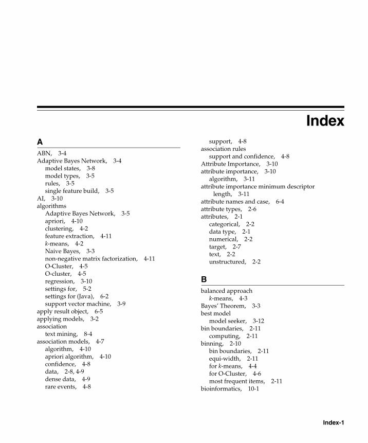
Index-1
IndexAABN, 3-4Adaptive Bayes Network, 3-4
model states, 3-8model types, 3-5rules, 3-5single feature build, 3-5
AI, 3-10algorithms
Adaptive Bayes Network, 3-5apriori, 4-10clustering, 4-2feature extraction, 4-11k-means, 4-2Naive Bayes, 3-3non-negative matrix factorization, 4-11O-Cluster, 4-5O-cluster, 4-5regression, 3-10settings for, 5-2settings for (Java), 6-2support vector machine, 3-9
apply result object, 6-5applying models, 3-2association
text mining, 8-4association models, 4-7
algorithm, 4-10apriori algorithm, 4-10confidence, 4-8data, 2-8, 4-9dense data, 4-9rare events, 4-8
support, 4-8association rules
support and confidence, 4-8Attribute Importance, 3-10attribute importance, 3-10
algorithm, 3-11attribute importance minimum descriptor
length, 3-11attribute names and case, 6-4attribute types, 2-6attributes, 2-1
categorical, 2-2data type, 2-1numerical, 2-2target, 2-7text, 2-2unstructured, 2-2
Bbalanced approach
k-means, 4-3Bayes’ Theorem, 3-3best model
model seeker, 3-12bin boundaries, 2-11
computing, 2-11binning, 2-10
bin boundaries, 2-11equi-width, 2-11for k-means, 4-4for O-Cluster, 4-6most frequent items, 2-11
bioinformatics, 10-1
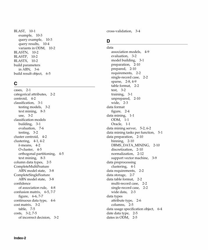
Index-2
BLAST, 10-1example, 10-3query example, 10-3query results, 10-4variants in ODM, 10-2
BLASTN, 10-2BLASTP, 10-2BLASTX, 10-2build parameters
in ABN, 3-6build result object, 6-5
Ccases, 2-1categorical attributes, 2-2centroid, 4-2classification, 3-1
testing models, 3-2text mining, 8-3use, 3-2
classification modelsbuilding, 3-1evaluation, 7-6testing, 3-2
cluster centroid, 4-2clustering, 4-1, 4-2
k-means, 4-2O-cluster, 4-5orthogonal partitioning, 4-5text mining, 8-3
column data types, 2-5CompleteMultiFeature
ABN model state, 3-8CompleteSingleFeature
ABN model state, 3-8confidence
of association rule, 4-8confusion matrix, 6-5, 7-7
figure, 6-6, 7-7continuous data type, 4-6cost matrix, 3-2
table, 7-5costs, 3-2, 7-5
of incorrect decision, 3-2
cross-validation, 3-4
Ddata
association models, 4-9evaluation, 3-2model building, 3-1preparation, 2-10prepared, 2-10requirements, 2-2single-record case, 2-2sparse, 2-8, 4-9table format, 2-2test, 3-2training, 3-1unprepared, 2-10wide, 2-3
data formatfigure, 2-4
data mining, 1-1ODM, 1-1Oracle, 1-1
data mining server, 5-2, 6-2data mining tasks per function, 5-1data preparation, 2-10
binning, 2-10DBMS_DATA_MINING, 2-10discretization, 2-10normalization, 2-12support vector machine, 3-9
data preprocessingclustering, 4-1
data requirements, 2-2data storage, 2-7data table format, 2-2
multi-record case, 2-2single-record case, 2-2wide data, 2-3
data typesattribute type, 2-6columns, 2-5
data usage specification object, 6-4date data type, 2-5dates in ODM, 2-5
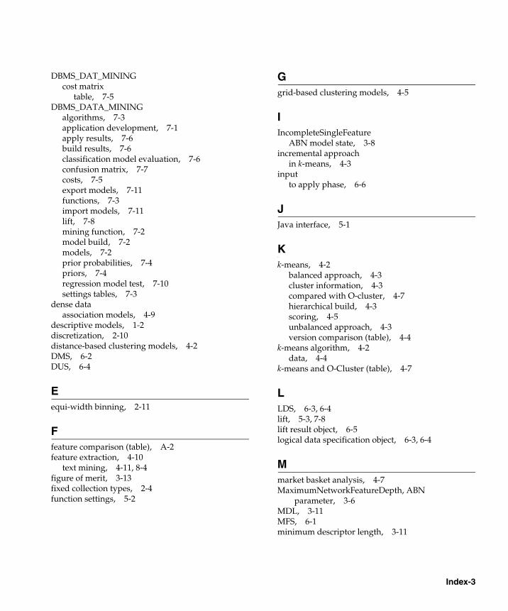
Index-3
DBMS_DAT_MININGcost matrix
table, 7-5DBMS_DATA_MINING
algorithms, 7-3application development, 7-1apply results, 7-6build results, 7-6classification model evaluation, 7-6confusion matrix, 7-7costs, 7-5export models, 7-11functions, 7-3import models, 7-11lift, 7-8mining function, 7-2model build, 7-2models, 7-2prior probabilities, 7-4priors, 7-4regression model test, 7-10settings tables, 7-3
dense dataassociation models, 4-9
descriptive models, 1-2discretization, 2-10distance-based clustering models, 4-2DMS, 6-2DUS, 6-4
Eequi-width binning, 2-11
Ffeature comparison (table), A-2feature extraction, 4-10
text mining, 4-11, 8-4figure of merit, 3-13fixed collection types, 2-4function settings, 5-2
Ggrid-based clustering models, 4-5
IIncompleteSingleFeature
ABN model state, 3-8incremental approach
in k-means, 4-3input
to apply phase, 6-6
JJava interface, 5-1
Kk-means, 4-2
balanced approach, 4-3cluster information, 4-3compared with O-cluster, 4-7hierarchical build, 4-3scoring, 4-5unbalanced approach, 4-3version comparison (table), 4-4
k-means algorithm, 4-2data, 4-4
k-means and O-Cluster (table), 4-7
LLDS, 6-3, 6-4lift, 5-3, 7-8lift result object, 6-5logical data specification object, 6-3, 6-4
Mmarket basket analysis, 4-7MaximumNetworkFeatureDepth, ABN
parameter, 3-6MDL, 3-11MFS, 6-1minimum descriptor length, 3-11
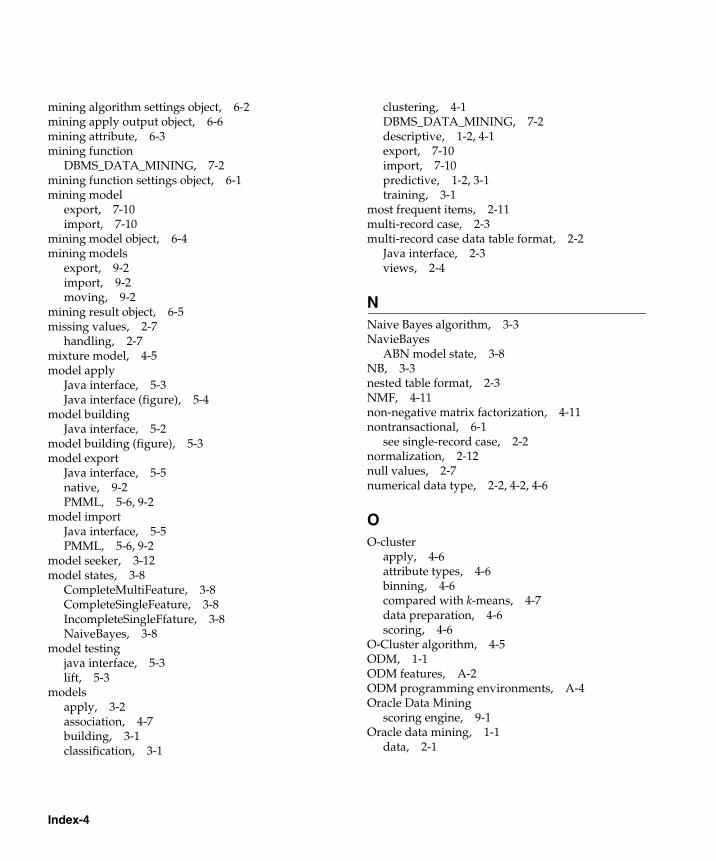
Index-4
mining algorithm settings object, 6-2mining apply output object, 6-6mining attribute, 6-3mining function
DBMS_DATA_MINING, 7-2mining function settings object, 6-1mining model
export, 7-10import, 7-10
mining model object, 6-4mining models
export, 9-2import, 9-2moving, 9-2
mining result object, 6-5missing values, 2-7
handling, 2-7mixture model, 4-5model apply
Java interface, 5-3Java interface (figure), 5-4
model buildingJava interface, 5-2
model building (figure), 5-3model export
Java interface, 5-5native, 9-2PMML, 5-6, 9-2
model importJava interface, 5-5PMML, 5-6, 9-2
model seeker, 3-12model states, 3-8
CompleteMultiFeature, 3-8CompleteSingleFeature, 3-8IncompleteSingleFfature, 3-8NaiveBayes, 3-8
model testingjava interface, 5-3lift, 5-3
modelsapply, 3-2association, 4-7building, 3-1classification, 3-1
clustering, 4-1DBMS_DATA_MINING, 7-2descriptive, 1-2, 4-1export, 7-10import, 7-10predictive, 1-2, 3-1training, 3-1
most frequent items, 2-11multi-record case, 2-3multi-record case data table format, 2-2
Java interface, 2-3views, 2-4
NNaive Bayes algorithm, 3-3NavieBayes
ABN model state, 3-8NB, 3-3nested table format, 2-3NMF, 4-11non-negative matrix factorization, 4-11nontransactional, 6-1
see single-record case, 2-2normalization, 2-12null values, 2-7numerical data type, 2-2, 4-2, 4-6
OO-cluster
apply, 4-6attribute types, 4-6binning, 4-6compared with k-means, 4-7data preparation, 4-6scoring, 4-6
O-Cluster algorithm, 4-5ODM, 1-1ODM features, A-2ODM programming environments, A-4Oracle Data Mining
scoring engine, 9-1Oracle data mining, 1-1
data, 2-1
Index-5
orthogonal partitioning clustering, 4-5outliers, 2-8
PPDS, 6-1physical data specification, 6-1PL/SQL interface
algorithms, 7-3functions, 7-3
PMML, 5-6export, 9-2import, 9-2Java interface, 5-6
Predictive Model Markup Language, 5-6predictive models, 1-2, 3-1prepared data, 2-10preprocessing
data, 4-1prior probabilities, 7-4priors, 3-3, 7-4programming environments, A-4
Rrare events
association models, 4-8receiver operating characteristics, 7-8
figure, 7-9statistics, 7-10
regression, 3-10algorithm, 3-10text mining, 8-4
regression modelstest, 7-10
ROC, 7-8rules
Adaptive Bayes Network, 3-5
Sscoring, 3-2, 4-5
in applications, 9-1O-Cluster, 4-6
scoring data, 3-2, 9-1
scoring engine, 9-1application deployment, 9-3features, 9-1installation, 9-1use, 9-3
sequence alignment, 10-1ODM capabilities, 10-2
sequence search, 10-1ODM capabilities, 10-2
setting tables, 7-3settings
support vector machine, 3-9single-record case, 2-3single-record case format, 2-2sparse data, 2-8, 4-9summarization, 4-7
in k-means, 4-5support
of association rule, 4-8support vector machine, 3-9
data preparation, 3-9regression, 3-10settings, 3-9
SVM, 3-9
Ttargets, 2-7TBLASTN, 10-2TBLASTX, 10-2test result object, 6-5testing models, 3-2
DBMS_DATA_MINING, 7-6text mining, 4-11, 8-1
association, 8-4classification, 8-3clustering, 8-3feature extraction, 4-11, 8-4ODM support, 8-1regression, 8-4support (figure), 8-5
transactional, 6-1see multi-record case, 2-3
Index-6
Uunbalanced approach
k-means, 4-3unprepared data, 2-10unstructured attributes, 2-2unstructured data, 2-5
Wwide data, 2-3
fixed collection types, 2-4nested table format, 2-3
winsorizing, 2-11figure, 2-12