Embed Size (px)
Citation preview

N. d’ordre : ...
Ecole Doctorale SPI de Lille Universite d’Artois
THESE DE DOCTORAT DE
L’UNIVERSITE D’ARTOIS
Specialite : Informatique et Automatique
Ecole doctorale SPI Lille Nord de France
Presentee par
M. Yamine BOUZEMBRAK
Pour obtenir le grade de
DOCTEUR de l’UNIVERSITE D’ARTOIS
Sujet de la these :
Conception des chaınes logistiques multicirteres avec
prise en compte des incertitudes
soutenue le 09/12/2011 devant le jury compose de :
M. El-Houssaine AGHEZZAF Examinateur
M. Hamid ALLAOUI Co-encadrant
M. Mohamed BAKLOUTI Co-directeur de these
Mme. Hanen BOUCHRIHA Co-encadrante
M. Alexandre DOLGUI Rapporteur
M. Gilles GONCALVES Co-directeur de these (Invite)
M. Samir LAMOURI Rapporteur
Laboratoire de Genie Informatique et d’Automatique de l’Artois (E.A. 3926)

Multi-criteria Supply Chain Network Design under
Uncertainty
Yamine BOUZEMBRAK
12 2011

Contents
1 Introduction 1
1.1 Problem statement . . . . . . . . . . . . . . . . . . . . . . . . . . . . . . . 5
1.2 Research Contribution . . . . . . . . . . . . . . . . . . . . . . . . . . . . . 5
1.3 Outline of Dissertation . . . . . . . . . . . . . . . . . . . . . . . . . . . . . 6
2 Literature Review on Supply Chain Network Design 9
2.1 Introduction . . . . . . . . . . . . . . . . . . . . . . . . . . . . . . . . . . . 9
2.2 Decision Levels . . . . . . . . . . . . . . . . . . . . . . . . . . . . . . . . . 10
2.2.1 Strategic level . . . . . . . . . . . . . . . . . . . . . . . . . . . . . . 11
2.2.2 Tactical Level . . . . . . . . . . . . . . . . . . . . . . . . . . . . . . 12
2.2.3 Operational Level . . . . . . . . . . . . . . . . . . . . . . . . . . . . 13
2.3 Supply Chain Network Structure . . . . . . . . . . . . . . . . . . . . . . . 14
2.4 Supply Chain Network Modelling Approaches . . . . . . . . . . . . . . . . 20
2.4.1 Deterministic SCND Models . . . . . . . . . . . . . . . . . . . . . . 20
2.4.2 SCND Models Under Uncertainty . . . . . . . . . . . . . . . . . . . 26
2.4.3 Resolution Methods . . . . . . . . . . . . . . . . . . . . . . . . . . . 37
2.5 Concluding Remarks . . . . . . . . . . . . . . . . . . . . . . . . . . . . . . 37
3 Multi-criteria Supply Chain Network Design 43
3.1 Introduction . . . . . . . . . . . . . . . . . . . . . . . . . . . . . . . . . . . 43
3.2 Problem description . . . . . . . . . . . . . . . . . . . . . . . . . . . . . . . 44
3.2.1 SCND evaluation criteria . . . . . . . . . . . . . . . . . . . . . . . . 45
3.2.2 Multi-modality in SCND . . . . . . . . . . . . . . . . . . . . . . . . 47
3.3 Approach presentation . . . . . . . . . . . . . . . . . . . . . . . . . . . . . 48
i

3.3.1 STEP 1: Multi-criteria selection model for potential facility locations 49
3.3.2 STEP 2: Mathematical model solving supply chain network design . 55
3.4 Case study . . . . . . . . . . . . . . . . . . . . . . . . . . . . . . . . . . . . 60
3.4.1 Supply Chain Network . . . . . . . . . . . . . . . . . . . . . . . . . 60
3.5 Application of the Approach . . . . . . . . . . . . . . . . . . . . . . . . . . 62
3.5.1 STEP 1: Multi-criteria selection model for potential facility location 62
3.5.2 STEP 2: Mathematical model solving supply chain network design . 71
3.6 Concluding remarks . . . . . . . . . . . . . . . . . . . . . . . . . . . . . . . 82
4 Multi-objective Supply Chain Network Design 83
4.1 Introduction . . . . . . . . . . . . . . . . . . . . . . . . . . . . . . . . . . . 84
4.2 Goal Programming . . . . . . . . . . . . . . . . . . . . . . . . . . . . . . . 85
4.2.1 Normalisation Techniques . . . . . . . . . . . . . . . . . . . . . . . 87
4.3 Problem Formulation . . . . . . . . . . . . . . . . . . . . . . . . . . . . . . 87
4.3.1 Mathematical Model . . . . . . . . . . . . . . . . . . . . . . . . . . 89
4.3.2 Goal Programming Model . . . . . . . . . . . . . . . . . . . . . . . 92
4.4 Computational Results . . . . . . . . . . . . . . . . . . . . . . . . . . . . . 94
4.4.1 Goal Programming weights . . . . . . . . . . . . . . . . . . . . . . . 95
4.4.2 Solutions . . . . . . . . . . . . . . . . . . . . . . . . . . . . . . . . . 95
4.4.3 Sensitivity Analysis . . . . . . . . . . . . . . . . . . . . . . . . . . . 96
4.5 Conclusions . . . . . . . . . . . . . . . . . . . . . . . . . . . . . . . . . . . 104
5 Heuristic Approach to large scale Supply Chain Network Design Prob-
lem 105
5.1 Introduction . . . . . . . . . . . . . . . . . . . . . . . . . . . . . . . . . . . 105
5.2 Mathematical Model . . . . . . . . . . . . . . . . . . . . . . . . . . . . . . 108
5.3 Heuristic Approach . . . . . . . . . . . . . . . . . . . . . . . . . . . . . . . 113
5.3.1 Heuristic Structure . . . . . . . . . . . . . . . . . . . . . . . . . . . 113
5.3.2 Decomposition Phase . . . . . . . . . . . . . . . . . . . . . . . . . . 115
5.3.3 Reduction Phase . . . . . . . . . . . . . . . . . . . . . . . . . . . . 116
5.3.4 Resolution Phase . . . . . . . . . . . . . . . . . . . . . . . . . . . . 118
5.4 Application Case . . . . . . . . . . . . . . . . . . . . . . . . . . . . . . . . 119
ii

5.4.1 Decomposition Phase . . . . . . . . . . . . . . . . . . . . . . . . . . 119
5.4.2 Reduction Phase . . . . . . . . . . . . . . . . . . . . . . . . . . . . 120
5.4.3 Resolution Phase . . . . . . . . . . . . . . . . . . . . . . . . . . . . 124
5.5 Computational Results . . . . . . . . . . . . . . . . . . . . . . . . . . . . . 125
5.5.1 Data and Implementation . . . . . . . . . . . . . . . . . . . . . . . 125
5.5.2 Performance of Heuristic . . . . . . . . . . . . . . . . . . . . . . . 126
5.5.3 Quality of Heuristic Solutions . . . . . . . . . . . . . . . . . . . . . 129
5.6 Concluding Remarks . . . . . . . . . . . . . . . . . . . . . . . . . . . . . . 140
6 Supply Chain Network Design under Uncertainty 141
6.1 Stochastic Supply Chain Network Design . . . . . . . . . . . . . . . . . . . 142
6.1.1 Introduction . . . . . . . . . . . . . . . . . . . . . . . . . . . . . . . 142
6.1.2 Model Development . . . . . . . . . . . . . . . . . . . . . . . . . . . 144
6.1.3 Computational results . . . . . . . . . . . . . . . . . . . . . . . . . 149
6.1.4 Concluding Remarks . . . . . . . . . . . . . . . . . . . . . . . . . . 153
6.2 Possibilistic Supply Chain Network Design . . . . . . . . . . . . . . . . . . 154
6.2.1 Introduction . . . . . . . . . . . . . . . . . . . . . . . . . . . . . . . 154
6.2.2 Possibilistic Linear Programming . . . . . . . . . . . . . . . . . . . 156
6.2.3 Model Development . . . . . . . . . . . . . . . . . . . . . . . . . . . 157
6.2.4 Application to the real case . . . . . . . . . . . . . . . . . . . . . . 166
6.2.5 Concluding Remarks . . . . . . . . . . . . . . . . . . . . . . . . . . 175
7 Conclusions and Perspectives 177
A Figures and Tables 182
A.1 AHP Example . . . . . . . . . . . . . . . . . . . . . . . . . . . . . . . . . . 182
A.2 Figures and Tables . . . . . . . . . . . . . . . . . . . . . . . . . . . . . . . 183
iii

List of Figures
1.1 Thesis structure diagram . . . . . . . . . . . . . . . . . . . . . . . . . . . . 6
2.1 Supply Chain Levels . . . . . . . . . . . . . . . . . . . . . . . . . . . . . . 10
2.2 Multi-criteria problems . . . . . . . . . . . . . . . . . . . . . . . . . . . . . 23
2.3 Uncertainty Modelling Methods . . . . . . . . . . . . . . . . . . . . . . . . 27
2.4 A scenario tree in two stage stochastic programming models . . . . . . . . 29
2.5 A scenario tree in multi-stage stochastic programming models . . . . . . . 29
3.1 Supply chain network . . . . . . . . . . . . . . . . . . . . . . . . . . . . . . 44
3.2 Sustainable supply chain network criteria . . . . . . . . . . . . . . . . . . . 46
3.3 Multi-criteria supply chain network design steps . . . . . . . . . . . . . . . 49
3.4 First step phases . . . . . . . . . . . . . . . . . . . . . . . . . . . . . . . . 50
3.5 Structure of GIS process . . . . . . . . . . . . . . . . . . . . . . . . . . . . 51
3.6 GIS Model . . . . . . . . . . . . . . . . . . . . . . . . . . . . . . . . . . . . 51
3.7 Raster Layers . . . . . . . . . . . . . . . . . . . . . . . . . . . . . . . . . . 52
3.8 AHP graphical representation . . . . . . . . . . . . . . . . . . . . . . . . . 53
3.9 Second step phases . . . . . . . . . . . . . . . . . . . . . . . . . . . . . . . 56
3.10 Supply chain network in NPDC region . . . . . . . . . . . . . . . . . . . . 61
3.11 Nature area classes in NPDC region . . . . . . . . . . . . . . . . . . . . . . 66
3.12 Hierarchical structure to the best selection of potential treatment facility
location in NPDC region . . . . . . . . . . . . . . . . . . . . . . . . . . . . 69
3.13 Potential treatment facility locations in NPDC region . . . . . . . . . . . . 70
3.14 Transportation modes in Nord Pas De Calais (NPDC) region . . . . . . . . 71
3.15 The transportation mode used varying ω1 . . . . . . . . . . . . . . . . . . . 75
3.16 Quantity of CO2 emission varying γ. . . . . . . . . . . . . . . . . . . . . . 78
iv

3.17 The transportation mode choose varying γ . . . . . . . . . . . . . . . . . . 79
4.1 Supply Chain Network . . . . . . . . . . . . . . . . . . . . . . . . . . . . . 88
4.2 Transportation mode used (%) . . . . . . . . . . . . . . . . . . . . . . . . . 98
4.3 Number of opened facilities . . . . . . . . . . . . . . . . . . . . . . . . . . 100
4.4 Total costs goal g1 variation . . . . . . . . . . . . . . . . . . . . . . . . . . 101
4.5 Energy Consumption Costs . . . . . . . . . . . . . . . . . . . . . . . . . . 103
4.6 CO2 emissions . . . . . . . . . . . . . . . . . . . . . . . . . . . . . . . . . . 104
5.1 Supply Chain Network . . . . . . . . . . . . . . . . . . . . . . . . . . . . . 109
5.2 n level supply chain network . . . . . . . . . . . . . . . . . . . . . . . . . . 114
5.3 Heuristic steps:Decomposition phase and Reduction phase . . . . . . . . . 115
5.4 p-median network . . . . . . . . . . . . . . . . . . . . . . . . . . . . . . . . 118
5.5 Supply Chain Network . . . . . . . . . . . . . . . . . . . . . . . . . . . . . 119
5.6 Decomposition phase . . . . . . . . . . . . . . . . . . . . . . . . . . . . . . 120
5.7 Heuristic steps: Decomposition phase and Reduction phase . . . . . . . . . 121
5.8 Step 1 . . . . . . . . . . . . . . . . . . . . . . . . . . . . . . . . . . . . . . 121
5.9 Step 2 . . . . . . . . . . . . . . . . . . . . . . . . . . . . . . . . . . . . . . 122
5.10 Step 3 . . . . . . . . . . . . . . . . . . . . . . . . . . . . . . . . . . . . . . 123
5.11 Step 4 . . . . . . . . . . . . . . . . . . . . . . . . . . . . . . . . . . . . . . 124
5.12 Step 5 . . . . . . . . . . . . . . . . . . . . . . . . . . . . . . . . . . . . . . 125
5.13 Constraints: MILP model vs Heuristic . . . . . . . . . . . . . . . . . . . . 127
5.14 Variables: MILP model vs Heuristic . . . . . . . . . . . . . . . . . . . . . . 128
5.15 CPU time: MILP model vs Heuristic . . . . . . . . . . . . . . . . . . . . . 128
6.1 Supply Chain Network . . . . . . . . . . . . . . . . . . . . . . . . . . . . . 144
6.2 Solution costs comparison . . . . . . . . . . . . . . . . . . . . . . . . . . . 152
6.3 Modelling and resolution method . . . . . . . . . . . . . . . . . . . . . . . 158
6.4 The triangular possibility distribution of cij . . . . . . . . . . . . . . . . . 159
6.5 Supply Chain Network . . . . . . . . . . . . . . . . . . . . . . . . . . . . . 162
6.6 Used budget level: Possibilistic vs Deterministic . . . . . . . . . . . . . . . 173
6.7 Used capacity level: Possibilistic vs Deterministic . . . . . . . . . . . . . . 173
6.8 Average service level: Possibilistic vs Deterministic . . . . . . . . . . . . . 174
v

6.9 Penality: Possibilistic vs Deterministic . . . . . . . . . . . . . . . . . . . . 175
A.1 Sediments depots in NPDC region . . . . . . . . . . . . . . . . . . . . . . . 184
A.2 Roads network classes in NPDC region . . . . . . . . . . . . . . . . . . . . 184
A.3 Railways network classes in NPDC region . . . . . . . . . . . . . . . . . . 185
A.4 Waterways network classes in NPDC region . . . . . . . . . . . . . . . . . 186
A.5 VNF landfills classes . . . . . . . . . . . . . . . . . . . . . . . . . . . . . . 186
A.6 Brownfield classes in NPDC region . . . . . . . . . . . . . . . . . . . . . . 187
A.7 GIS Model . . . . . . . . . . . . . . . . . . . . . . . . . . . . . . . . . . . . 191
vi
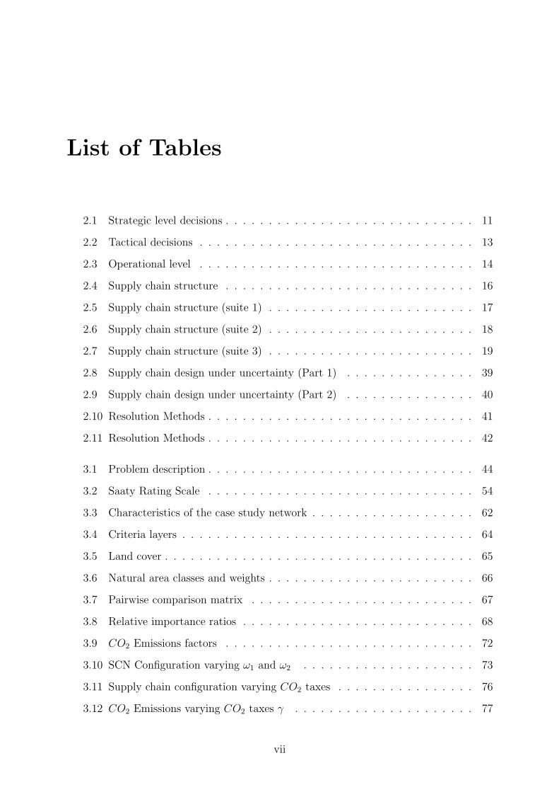
List of Tables
2.1 Strategic level decisions . . . . . . . . . . . . . . . . . . . . . . . . . . . . . 11
2.2 Tactical decisions . . . . . . . . . . . . . . . . . . . . . . . . . . . . . . . . 13
2.3 Operational level . . . . . . . . . . . . . . . . . . . . . . . . . . . . . . . . 14
2.4 Supply chain structure . . . . . . . . . . . . . . . . . . . . . . . . . . . . . 16
2.5 Supply chain structure (suite 1) . . . . . . . . . . . . . . . . . . . . . . . . 17
2.6 Supply chain structure (suite 2) . . . . . . . . . . . . . . . . . . . . . . . . 18
2.7 Supply chain structure (suite 3) . . . . . . . . . . . . . . . . . . . . . . . . 19
2.8 Supply chain design under uncertainty (Part 1) . . . . . . . . . . . . . . . 39
2.9 Supply chain design under uncertainty (Part 2) . . . . . . . . . . . . . . . 40
2.10 Resolution Methods . . . . . . . . . . . . . . . . . . . . . . . . . . . . . . . 41
2.11 Resolution Methods . . . . . . . . . . . . . . . . . . . . . . . . . . . . . . . 42
3.1 Problem description . . . . . . . . . . . . . . . . . . . . . . . . . . . . . . . 44
3.2 Saaty Rating Scale . . . . . . . . . . . . . . . . . . . . . . . . . . . . . . . 54
3.3 Characteristics of the case study network . . . . . . . . . . . . . . . . . . . 62
3.4 Criteria layers . . . . . . . . . . . . . . . . . . . . . . . . . . . . . . . . . . 64
3.5 Land cover . . . . . . . . . . . . . . . . . . . . . . . . . . . . . . . . . . . . 65
3.6 Natural area classes and weights . . . . . . . . . . . . . . . . . . . . . . . . 66
3.7 Pairwise comparison matrix . . . . . . . . . . . . . . . . . . . . . . . . . . 67
3.8 Relative importance ratios . . . . . . . . . . . . . . . . . . . . . . . . . . . 68
3.9 CO2 Emissions factors . . . . . . . . . . . . . . . . . . . . . . . . . . . . . 72
3.10 SCN Configuration varying ω1 and ω2 . . . . . . . . . . . . . . . . . . . . 73
3.11 Supply chain configuration varying CO2 taxes . . . . . . . . . . . . . . . . 76
3.12 CO2 Emissions varying CO2 taxes γ . . . . . . . . . . . . . . . . . . . . . 77
vii

3.13 Transportation modes used varying CO2 taxes . . . . . . . . . . . . . . . . 77
3.14 Low demand case . . . . . . . . . . . . . . . . . . . . . . . . . . . . . . . . 80
3.15 Medium demand case . . . . . . . . . . . . . . . . . . . . . . . . . . . . . . 81
3.16 High demand case . . . . . . . . . . . . . . . . . . . . . . . . . . . . . . . . 81
4.1 The Goal Programming weights . . . . . . . . . . . . . . . . . . . . . . . . 95
4.2 Solutions . . . . . . . . . . . . . . . . . . . . . . . . . . . . . . . . . . . . . 97
4.3 Sensitivity . . . . . . . . . . . . . . . . . . . . . . . . . . . . . . . . . . . . 99
4.4 Total costs goal g1 variation . . . . . . . . . . . . . . . . . . . . . . . . . . 100
4.5 Energy consumption goal g2 variation . . . . . . . . . . . . . . . . . . . . . 102
4.6 CO2 emissions goal g4 variation . . . . . . . . . . . . . . . . . . . . . . . . 103
5.1 Global MILP model limits . . . . . . . . . . . . . . . . . . . . . . . . . . . 112
5.2 Constraints and variables numbers: Heuristic vs Global MILP model . . . 130
5.3 CPU time: Heuristic vs Global MILP model . . . . . . . . . . . . . . . . . 131
5.4 Solutions: Heuristic vs Global MILP model . . . . . . . . . . . . . . . . . . 133
5.5 Configuration: Heuristic vs Global MILP (Part 1) . . . . . . . . . . . . . . 134
5.6 Configuration: Heuristic vs Global MILP (Part 2) . . . . . . . . . . . . . . 135
5.7 Configuration: Heuristic vs Global MILP (Part 3) . . . . . . . . . . . . . . 136
5.8 Configuration: Heuristic vs Global MILP (Part 4) . . . . . . . . . . . . . . 137
5.9 Configuration: Heuristic vs Global MILP (Part 5) . . . . . . . . . . . . . . 138
5.10 Configuration: Heuristic vs Global MILP (Part 6) . . . . . . . . . . . . . . 139
6.1 Computational Results . . . . . . . . . . . . . . . . . . . . . . . . . . . . . 150
6.2 Comparison of Deterministic cost to Stochastic cost. . . . . . . . . . . . . . 151
6.3 Comparison of optimal Deterministic solutions to worst case solutions. . . 151
6.4 Comparison of Stochastic cost to worst case cost. . . . . . . . . . . . . . . 152
6.5 α-acceptable optimal solutions (part 1) . . . . . . . . . . . . . . . . . . . . 168
6.6 α-acceptable optimal solutions (Part 2) . . . . . . . . . . . . . . . . . . . . 169
6.7 Computational Results . . . . . . . . . . . . . . . . . . . . . . . . . . . . . 170
6.8 Experiments . . . . . . . . . . . . . . . . . . . . . . . . . . . . . . . . . . . 171
6.9 Possibilistic vs Deterministic Results . . . . . . . . . . . . . . . . . . . . . 172
viii

A.1 Comparison between criteria . . . . . . . . . . . . . . . . . . . . . . . . . . 183
A.2 Relative importance ratios . . . . . . . . . . . . . . . . . . . . . . . . . . . 183
A.3 Roads network classes and weights . . . . . . . . . . . . . . . . . . . . . . 184
A.4 Railways network classes and weights . . . . . . . . . . . . . . . . . . . . . 185
A.5 Waterways network classes and weights . . . . . . . . . . . . . . . . . . . 185
A.6 Landfills classes and weights . . . . . . . . . . . . . . . . . . . . . . . . . . 187
A.7 Brownfield classes and weights . . . . . . . . . . . . . . . . . . . . . . . . . 187
A.8 Supply chain configuration varying CO2 taxes . . . . . . . . . . . . . . . . 188
A.9 CO2 Emissions varying CO2 taxes . . . . . . . . . . . . . . . . . . . . . . . 189
A.10 Transportation modes used varying CO2 taxes . . . . . . . . . . . . . . . 190
A.11 Law demand case . . . . . . . . . . . . . . . . . . . . . . . . . . . . . . . . 192
A.12 Medium demand case . . . . . . . . . . . . . . . . . . . . . . . . . . . . . . 193
A.13 High demand case . . . . . . . . . . . . . . . . . . . . . . . . . . . . . . . . 194
ix

Abstract
This thesis contributes to the debate on how uncertainty and concepts of sustainable de-
velopment can be put into modern supply chain network and focuses on issues associated
with the design of multi-criteria supply chain network under uncertainty.
First, we study the literature review , which is a review of the current state of the art of
Supply Chain Network Design approaches and resolution methods.
Second, we propose a new methodology for multi-criteria Supply Chain Network Design
(SCND) as well as its application to real Supply Chain Network (SCN), in order to satisfy
the customers demand and respect the environmental, social, legislative, and economical
requirements. The methodology consists of two different steps. In the first step, we use
Geographic Information System (GIS) and Analytic Hierarchy Process (AHP) to build
the model. Then, in the second step, we establish the optimal supply chain network using
Mixed Integer Linear Programming model (MILP).
Third, we extend the MILP to a multi-objective optimization model that captures a com-
promise between the total cost and the environment influence. We use Goal Programming
approach seeking to reach the goals placed by Decision Maker. After that, we develop
a novel heuristic solution method based on decomposition technique, to solve large scale
supply chain network design problems that we failed to solve using exact methods. The
heuristic method is tested on real case instances and numerical comparisons show that
our heuristic yield high quality solutions in very limited CPU time.
Finally, again, we extend the MILP model presented before where we assume that the
costumer demands are uncertain. We use two-stage stochastic programming approach
to model the supply chain network under demand uncertainty. Then, we address uncer-
tainty in all SC parameters: opening costs, production costs, storage costs and customers
demands. We use possibilistic linear programming approach to model the problem and
we validate both approaches in a large application case.

Chapter 1
Introduction
In 1915, Arch Shaw (1915) pointed out that: ” The relations between the activities of
demand creation and physical supply...illustrated the existence of the two principles of
interdependence and balance. Failure to co-ordinate any one of these activities with its
group-fellows and also with those in the other group, or undue emphasis or outlay put on
any one of these activities, is certain to set the equilibrium of forces which means efficient
distribution... The physical distribution of the goods is a problem distinct from the cre-
ation of demand...Not a few worthy failures in distribution campaigns have been due to
such a lack of co-ordination between demand creation and physical supply.”
It has taken more than 70 years the principals of Supply Chain Management (SCM) to be
clearly defined in literature : according to Jones and Riley (1985), supply chain manage-
ment is an integrative approach to dealing with the planning and control of the materials
flow from suppliers to end-users. In Berry et al (1994), the SCM aims at building trust,
exchanging information on market needs, developing new products, and reducing the sup-
plier base to a particular original equipment manufacturer so as to release management
resources for developing meaningful, long term relationship.
Tan et al. (1998) integrated the recycling step in the definition of SCM, it encompasses
materials/supply management from the supply of basic raw materials to final product (and
possible recycling and re-use). Supply chain management focuses on how firms utilize their
suppliers’ processes, technology and capability to enhance competitive advantage. It is
a management philosophy that extends traditional intra enterprise activities by bringing
trading partners together with the common goal of optimization and efficiency.
1
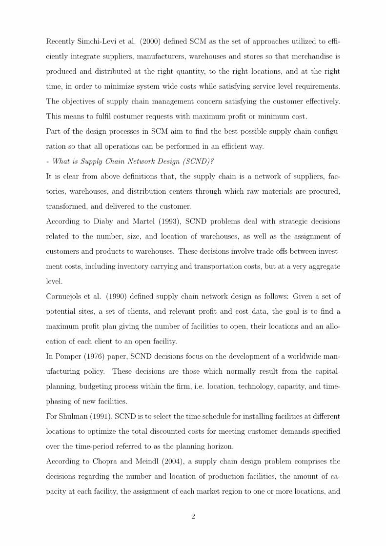
Recently Simchi-Levi et al. (2000) defined SCM as the set of approaches utilized to effi-
ciently integrate suppliers, manufacturers, warehouses and stores so that merchandise is
produced and distributed at the right quantity, to the right locations, and at the right
time, in order to minimize system wide costs while satisfying service level requirements.
The objectives of supply chain management concern satisfying the customer effectively.
This means to fulfil costumer requests with maximum profit or minimum cost.
Part of the design processes in SCM aim to find the best possible supply chain configu-
ration so that all operations can be performed in an efficient way.
- What is Supply Chain Network Design (SCND)?
It is clear from above definitions that, the supply chain is a network of suppliers, fac-
tories, warehouses, and distribution centers through which raw materials are procured,
transformed, and delivered to the customer.
According to Diaby and Martel (1993), SCND problems deal with strategic decisions
related to the number, size, and location of warehouses, as well as the assignment of
customers and products to warehouses. These decisions involve trade-offs between invest-
ment costs, including inventory carrying and transportation costs, but at a very aggregate
level.
Cornuejols et al. (1990) defined supply chain network design as follows: Given a set of
potential sites, a set of clients, and relevant profit and cost data, the goal is to find a
maximum profit plan giving the number of facilities to open, their locations and an allo-
cation of each client to an open facility.
In Pomper (1976) paper, SCND decisions focus on the development of a worldwide man-
ufacturing policy. These decisions are those which normally result from the capital-
planning, budgeting process within the firm, i.e. location, technology, capacity, and time-
phasing of new facilities.
For Shulman (1991), SCND is to select the time schedule for installing facilities at different
locations to optimize the total discounted costs for meeting customer demands specified
over the time-period referred to as the planning horizon.
According to Chopra and Meindl (2004), a supply chain design problem comprises the
decisions regarding the number and location of production facilities, the amount of ca-
pacity at each facility, the assignment of each market region to one or more locations, and
2

supplier selection for sub-assemblies, components and materials.
Many researchers have attempted to extend these classical definitions by incorporating
various themes such as: sustainability of supply chains has emerged since the impacts
of climate change have effected producers and consumers decision-making and how their
decisions effect the environment, transportation modes, tax issue and risk management,
etc.
As the competitive context of business continues to change, bringing with it new complex-
ities and concerns for management generally, it also has to be recognized that the impact
of these changes on logistics can be considerable. Indeed, perhaps the most challenging
strategic issues that confront the business organization today are in the area of Supply
Chain (SC), which are: (i) the customer service, (ii) time compression, (iii) globalization
and (iv) organization.
- The customer service:
Nowadays, the customer is more demanding, not just of product price and product qual-
ity, but also of service. As more and more the technical difference between offers decrease,
products don’t have value until they are in the hands of the customer at the time and
place required. In other words, customer needs for the creation of added value through
customer service (Christopher (2001)). To achieve this, a company may be able to save
millions of Euro in logistic costs and simultaneously improve service levels by redesigning
or designing its supply chain network.
- Time compression:
In recent years, time has become a critical issue in supply chain management. Logis-
tic actors require just-in-time deliveries, products life cycle and order cycles are shorter
than ever and customers accept a competitor product if their first choice is not instantly
available. To overcome these problems and ensure timely response to volatile and uncer-
tain demand, new approaches to the management of lead times are required (Christopher
(2001)). Neglecting uncertainty in supply chain network design may cause more than high
costs on the long term objectives of a company Santoso et al. (2005), Klibi et al. (2010),
Sabri and Beamon (2000). Building a sustainable supply chain nowadays has become the
ultimate objective of intelligent organisations.
- Globalization:
3
In the global business materials and components are sourced worldwide, manufactured
offshore in many different countries perhaps with local customization. However, experts
maintain that global supply chains are more difficult to manage than domestic supply
chains (Wood et al. (2002), MacCarthy and Atthirawong (2003)). Geographical dis-
tances in these global situations not only increase transportation costs, but also inventory
costs and lead-time in the supply chain. Different local cultures, languages, and prac-
tices reduce the effectiveness of demand forecasting and material planning. Deficiencies
in transportation and telecommunication infrastructures, as well as inadequate worker
skills, supplier quality, equipment and technology provide challenges normally not expe-
rienced in developed countries.
For global companies, the management of supply chain has become an issue of central
concern. They seek to achieve competitive advantage by identifying world markets for
their products then developing a supply chain strategy to support their marketing strat-
egy (Christopher (2001)).
Indeed, the ultimate objective in supply chain network design should be not only to
minimize common costs, but also to integrate multi-criteria in the SCND and to reduce
vulnerability due to uncertainty , by reducing possible sources of lose due to uncertainty.
- Organisation:
The classical business organization is based on strict functional divisions and hierarchies,
where each manager manages each own function independently from others. In today’s
environment, the company organisation needs broad-based integrators which are oriented
to achieve marketplace success based on managing processes and people that deliver ser-
vice. Generalist and specialist managers are required to integrate materials management
with operational management and delivery. They will focus on customer service to achieve
the integration of functions (Christopher (2001)).
To achieve this, an ideal network must have the optimum number, size, and location of
warehouses to support the inventory replenishment activities of its retailers. This state-
ment calls for sophisticated facility location models to determine the best supply chain
configuration.
4

1.1 Problem statement
The main concepts that we focus on this thesis are the considerations of multi-criteria
Supply Chain Network Design (SCND), the uncertain environment in SCD and heuristic
algorithm to solve large size SCND problems.
We consider a multi-criteria, multi-level, single product, single period and multi-modal
(roads, railways, waterways) supply chain network problem. The network has four levels:
suppliers, storage depots or warehouses, production plants or distribution centers and
customers.
In this context, this research deals with the design of a sustainable supply chain network
under uncertain environment in order to satisfy the customers demand and to respect
the environmental, social, legislative, and economical requirements. The strategic supply
chain network we intend to establish, should answer the following questions under un-
certain environment: (i) how many facilities (manufacturing plants, warehouses or/and
distribution centers) should be installed? (ii) where the new sites should be located? (iii)
how much goods should each warehouse and/or distribution center handle? (iv) which
sellers should be served by each distribution centers? (v) products quantities to transport
throughout the supply chain network? (vi) which transportation mode should be used?
1.2 Research Contribution
According to what is presented previously, the main contributions of this research can be
summarized under five headings:
(1) A review of approaches and resolutions methods taking into account multi-criteria
and uncertainty in supply chain network design problems.
(2) A new methodology to design multi-criteria supply chain networks and applying the
model to a real-world treatment sediment supply chain. Geographic Information System
(GIS), Analytic Hierarchy Process (AHP) and Mixed Integer Linear Programming ap-
proaches are combined together to design the SCN.
(3) A new heuristic algorithm to solve large scale supply chain network problems and
applying the heuristic to a real-word textile supply chain (European Textile Company.
The heuristic is based on a decomposition technique.
5

(4) A two-stage stochastic programming approach for supply chain network design under
demand uncertainty. This proposal is tested by using data from a real Textile supply
chain.
(5) A possibilistic linear programming based approach for supply chain network design
in an uncertain environment. This model is validated by using data from a real-world
supply chain. The detail of these headings is outlined in the following.
1.3 Outline of Dissertation
This thesis is organised into 7 chapters and is presented according to the following dia-
gram (Figure 1.1).
This introductory Chapter is followed by the literature review in Chapter 2, which
Figure 1.1: Thesis structure diagram
is a review of the current state of the art of Supply Chain Network Design approaches
and resolution methods. Among other things, we recall the different decision levels in
Supply Chain (strategic, tactical and operational level), the supply chain network struc-
6

ture (single/multiple layer(s), single/multiple product(s), single/multiple period(s), sin-
gle/multiple objective (s), single/multiple modality, deterministic/stochastic parameters)
and existing deterministic SCND models and SCND models under uncertainty. We end
the chapter with some concluding remarks.
In order to satisfy the customers demand and to respect the environmental, social, leg-
islative, and economical requirements, a novel framework for multi-criteria Supply Chain
Network Design (SCND) and its application to real Supply Chain Network (SCN) are
presented in Chapter 3. The methodology consists of two different steps. The first step
looks for the best potential facility locations to open in order to satisfy the different cri-
teria: environmental, social, and legislation aspects, using the Geographic Information
System (GIS) and Analytic Hierarchy Process (AHP). The second step looks for the opti-
mal supply chain design to satisfy customer demands and economic criteria using mixed
integer linear programming model. The objective in this step is to determine location of
treatment facilities and their capacities minimizing the sum of : opening facilities cost,
products storage cost, production cost, transportation cost, and CO2 emissions taxes.
We apply our methodology to a real application case concerning the recycling of sediment
waterways, which was presented in Bouzembrak et al. (2010). We end the Chapter with
some concluding remarks.
In Chapter 4, we extend the second step of our methodology that we developed in
Chapter 3. We study a supply chain network design problem with environmental con-
cerns. We are interested in the environmental investments decisions in the design phase
and propose a multi-objective optimization model that captures a compromise between
the total cost and the environment influence. We use Goal Programming approach seek-
ing to reach the four goals placed by Decision Maker: (i) total costs goal, (ii) energy
consumption costs goal, (iii) waste treatment costs goal and (iv) CO2 emissions goal.
The strategic decisions considered in the model are facilities location, building technology
selection and flow of materials throughout the SC. We present numerical results illus-
trating and comparing the performance of the GP model, the instances elaborated from
the real application case presented in Chapter 3. We conclude the chapter with some
7

conclusions from our study.
In Chapter 5, a novel heuristic solution method is developed based on a decomposi-
tion technique, to solve large scale supply chain network design problems that we failed to
solve using exact methods. The heuristic method is tested on real case instances, Euro-
pean Textile Company, and it is compared to an exact method in solving small instances.
Computational tests with up to 1 500 customers, 220 potential warehouses, 220 potential
distribution centers and 220 suppliers are reported.
For the general model, a numerical comparison of the heuristic solutions to the exact
method solutions shows that the heuristics yield high quality solutions in very limited
time. We conclude the chapter with some conclusions from our study.
The deterministic model discussed in the previous chapter provides a base for Sup-
ply Chain Network Design (SCND). Nevertheless, any network design obtained based on
this model, which represents the optimal deterministic configuration, has no assurance
of performance for any other future parameter fluctuation. However, we extended the
deterministic model presented in chapter 3. We first assume that we got the statistical
data of the customer demands, so, we use two-stage stochastic programming approach to
model the supply chain network under demand uncertainty. After that, we address uncer-
tainty in all SC parameters: opening costs, production costs, storage costs and customers
demands. In the case where the statistical data of all these parameters are not available,
we use possibilistic linear programming approach to model the problem and we validate
the approach in a large real case textile supply chain network.
Finally, Chapter 7 concludes the research findings and the activities undertaken through-
out the thesis.
8

Chapter 2
Literature Review on Supply Chain
Network Design
In this chapter existing Supply Chain Network (SCN) modelling approaches and resolution
methods in literature will be discussed. In section 2.2, we show the different decision levels
in Supply Chain (SC) : strategic, tactical and operational level. Then, in section 2.3, we
recapitulate the supply chain network structure. In section 2.4, we introduce the most
important approaches used in Supply Chain Network Design (SCND). We end the chapter
in section 2.5 with some concluding remarks.
2.1 Introduction
Most articles on supply chain management include different form of categorization for lo-
gistic decisions (Ballou (2004), Bowersox et al. (2002), Chopra and Meindl (2004), Coyle
et al. (2003), Johnson et al (1999), Simchi-Levi et al. (2003)). These works generally
enumerate the logistic functions, indicate that many of decisions are interdependent and
present in detail models for solving various problems. Huang et al. (2003) considered
four classification criteria: supply chain structure, decision level, modelling approach and
shared information.
In this chapter we propose three classification criteria: decision level, supply chain net-
work structure and modelling approaches used on SCND. All of them are briefly described
below:
9

- Decision level: three decision levels may be distinguished in term of the decision to be
made; strategic, tactical and operational.
- Supply chain network structure: it defines the features that may be included in a SCN
model : single/multiple layer(s), single/multiple product(s), single/multiple period(s),
single/multiple objective (s), single/multiple modality, deterministic/stochastic parame-
ters.
- Supply chain network modelling approach: it consists in the type of representation,
mathematical relationship, and the aspects to be considered in the supply chain. Also, it
resumes the resolution methods that may be used in solving supply chain network models.
These categories will be detailed in the following sections.
2.2 Decision Levels
The decision making process in supply chain networks is highly complex. It can be
decomposed according to the time horizons considered (Gupta and Maranas, 1999). This
process results in the following temporal classification of the models: strategic, tactical and
operational. Figure 2.1 describes the different decision levels in supply chain management.
�
Control�
decisions
Material�flow��
decisions
Design�decisions
Operational
Tactical
Strategic
Figure 2.1: Supply Chain Levels
As we can see, strategic level decisions determine the configuration of the supply chain,
tactical level decisions prescribe material flow management and operational level decisions
present control decisions. The following paragraphs give the definitions of these levels.
10

2.2.1 Strategic level
This section addresses strategic level decisions, which determine the configuration of the
supply chain by prescribing supplier selection, facility location (plants, warehouses, dis-
tribution centers and costumers zones), production technologies, plant capacities and
transportation modes. Simchi-Levi et al. (2004) state that the strategic level deals with
decisions that have a long-lasting effect on the firm. These include decisions regarding the
number, location and capacities of warehouses and manufacturing plants, or the flow of
material through the logistic network. The main strategic questions addressed in SCND
approach are presented in the following Table 2.1:
In strategic phase, generally, the planners are not constrained by existing resources. The
Table 2.1: Strategic level decisions
Strategic Decisions Strategic Questions
Type and number How many production and Distribution Centers (DC)
should be implemented?
of facilities Which activities should be externalized?
Which products should be produced/stocked in each loca-
tion?
Size of facilities What production, storage and handling technologies should
we adopt and how much capacity should we have?
Facility location Where should they be located?
Supplier selection Which supplier should be selected?
Activities from each facility Which factory/DC/demand zones should be supplied by
each supplier/factory/DC?
What delivery time should we provide in different product
markets and at what price?
Utilisation of facilities Which factory/DC/Warehouse should be opened or closed?
Transportation Modes What means of transportation should be used (road, train,
waterways,...etc. )?
data used in this phase are often imprecise. Moreover, an operating plan must be con-
structed to assess various scenarios depending on the forecasts. Many factors contribute
11

to the complexity of SCN decision models. The first one is the long-term impact of the
design decisions. It may be reasonable to use one year model when the decisions are
limited to the selection of warehouses or distribution centers, as most of the literature
suggests.
A second complexity factor is uncertainty. Most models proposed in the literature are
deterministic. The interested reader can find these strategic questions in some important
works on supply chain network design: ReVelle and Eiselt (2005), Daskin et al. (2005),
Vila et al. (2006), Martel (2005), Klose and Drexl (2005), Arntzen et al. (1995), Cordeau
et al. (2006), Amiri (2005), Amrani et al. (2005), Ghiani et al. (2004). In stochastic
strategic supply chain design, you can find Santoso et al. (2005) and Shapiro (2001).
Furthermore, many references considered aspects related to the strategical and tactical
levels simultaneously (Dogan and Goetschalckx (1999), Jayaraman and Pirkul (2001),
Goetschalckx et al. (2002), Jang et al. (2002)).
2.2.2 Tactical Level
On the tactical level, medium term decisions are made. They are related to the flow
of materials between the supply chain actors, such as materials requirement planning,
production planning, inventory planning, transport capacities, inventories and managing
safety inventories and distribution planning (Table 2.2).
At this level, the policies and decisions not only aim to an adequate allocation and utiliza-
tion of existing resources, but also strive to achieve the best trade-off between benefits and
service performance. Furthermore, they are commonly used to model and analyse differ-
ent scenarios, such as determining the incremental operating costs or inventory quantities
for a set of volume changes. They are somewhat sensitive only to broad variations in
data. Midterm tactical models are intermediate in nature and incorporate some features
from both the strategic and operational models (Gupta and Maranas (2003)).
The main tactical decisions related to the supply chain management are recapitulated
in Table 2.2. Some works focus on the tactical decision level (Sabri and Beamon (2000),
Timpe and Kallrath (2000), Kallrath (2002), Liang and Cheng (2008), Torabi and Hassini
(2008) and Chen and Lee (2004)).
12

Table 2.2: Tactical decisions
Tactical Decisions Tactical Questions
Material requirement Which raw material supplier should be selected?
planning Which raw material should be selected?
How much raw materiel should be supplied from each supplier?
Production planning Which products should be produced?
How much goods should they be produced?
When should they be produced? On which machine?
Where should they be produced?
Inventory planning How much products should be stored?
Where should they be stored?
When should they be stored?
How should the cost of storing inventory be reduced?
Distribution planning Which plant to supply which distribution centers?
2.2.3 Operational Level
Operational level decisions involve shorter term horizon, generally one or several days,
and smaller area than the tactical level and strategic level decisions. They include a
wide variety of operational problems such as: demand forecasting, production, warehous-
ing, inventory management, transportation, product packaging, procurement and supply
management, etc. Particularly, real-time control problems are solved in real time during
operations and aim to minimize customer inconvenience.
In this level, the time factor plays a highly dynamic role. Notably, sometimes emergency
management is regarded as real-time level in the operation process. Table 2.3 classifies
the most important questions reviewed in terms of the operational decisions level.
Rizk et al. (2006, 2008) cover the operational decision level exclusively. The interested
reader can find operational models in some important works: the vehicle routing problem
(Eksioglu et al. (2009)), inventory management (Andersson et al. (2010)) and production
scheduling (Eren Akyol and Bayhan (2007)).
In the context of this thesis, we focus on the strategic supply chain network design. The
strategic SCN we intend to elaborate should answer the following strategic questions: (i)
13

Table 2.3: Operational level
Operational Decisions Operational Questions
Demand forecasting Quantities of future demand?
When should the future demand be received?
Where should be the future demand?
Production Where the product should be completed?
Who should produce the product?
Which layout of production facilities should be selected?
Which master production schedule should be selected?
Warehousing Which warehouse layout should be selected?
Where in the warehouse should each item stored?
What should be the storage policy of each item?
Inventory management Which methods should be used for controlling inventories?
Which should be the inventory levels?
The safety stock?
Transportation Which carrier type should be selected?
Vehicle routing and scheduling?
Assignment of customers to vehicles?
Product packaging Which type of packaging should be selected?
Which information should be provided with the product?
what type and how many facilities should be installed? (ii) where the new sites should be
established? (iii) how much goods should each plant handle? (iv) which transportation
mode should be used?
2.3 Supply Chain Network Structure
In supply chains, many basic features are included in strategic supply chain configura-
tion: single/multiple layer(s), single/multiple product(s), single/multiple period(s), sin-
gle/multiple objective (s), single/multiple modality, deterministic/stochastic parameters.
We conducted a detailed literature survey for the last decade period to reveal the current
14

state of art in SCND literature. The main review used to elaborate this work are (Melo
et al. (2009), Klibi et al. (2010), Kabak and Ulengin (2010), Meixell and Gargeya (2005),
Vidal and Goetschalckx (1997), Goetschalckx et al. (2002), Farahani et al. (2010) and
Strivastava (2007)). Table 2.7 classifies the surveyed literature according to these aspects.
It can be seen from Table 2.7 that the single product literature in SCND is approximately
equal to the multiple products one. Around 52% of papers presented include the single
product aspect. (Aghezzaf (2005), Barros et al. (1998), Daskin et al. (2002), Shu et al.
(2005), Tushaus and Wittmann (1998)).
The most of papers in SCND deal with single-period problem. Approximately 83% of the
surveyed papers present single-period model. (Vidal and Goetschalckx (2001), Yan et al.
(2003), Pirkul and Jayaraman (1998), Sabri and Beamon (2000), Santoso et al. (2005)).
Further, the number of multi-layer models are scarce compared with the one or two layers
models. Approximately 66% of the surveyed papers refer to two layers problem. (Melo
et al. (2006), Pati et al. (2008), Santoso et al. (2005), Wilhelm et al. (2005)).
Another important conclusion that can be drawn from Table 2.7 refers to the large num-
ber of deterministic models when compared with stochastic ones. Approximately 79%
of the literature in SCND refers to deterministic models. As pointed out by Sabri and
Beamon (2000), uncertainty is one of the most challenging problems in SCND. However,
the literature integrating uncertainty with location decisions in an SCND context is still
scarce (Van Ommeren et al. (2006), Sabri and Beamon (2000), Santoso et al. (2005),
Hwang (2002), Listes and Dekker (2005)).
The surveyed literature can also be divided into those papers that consider single-objective
problem and those that propose multiple-objective problem. The small number of papers
in this Table refers to models with multiple objective (approximately 10% against 90%).
(Melachrinoudis et al. (2005), Sabri and Beamon (2000), Altiparmak et al. (2006), Fara-
hani and Asgari (2007)). The last and smallest group of articles integrating decisions
regarding transportation modes, in strategic planning level, show that the existing lit-
erature is still far from combining many aspects relevant to SCND (approximately 7%
against 93%). In fact, this integration leads to much more complex models due to the
large size of problems that may results. (Carlsson and Ronnqvist (2005), Cordeau et al.
(2006), Eskigun et al. (2005)).
15

Table 2.4: Supply chain structure
Product Period Layer Model Objective Transportation Mode
Authors Single Multiple Single Multiple Two Multiple Deterministic Stochastic Single Multiple Single Multiple
Aghezzaf (2005) X X X X X X
Altiparmak et al. (2006) X X X X X X
Ambrosino and Scutell (2005) X X X X X X
Amiri et al. (2006) X X X X X X
Barros et al. (1998) X X X X X X
Carlsson and Ronnqvist (2005) X X X X X X
Cordeau et al. (2006) X X X X X X
Daskin et al. (2002) X X X X X X
Dogan and Goetschalckx (1999) X X X X X X
Erlebacher and Meller (2000) X X X X X X
Eskigun et al. (2005) X X X X X X
Guillen et al. (2005) X X X X X X
Gunnarsson et al. (2004) X X X X X X
Hinojosa et al. (2000) X X X X X X
16

Table 2.5: Supply chain structure (suite 1)
Product Period Layer Model Objective Transportation Mode
Authors Single Multiple Single Multiple Two Multiple Deterministic Stochastic Single Multiple Single Multiple
Hinojosa et al. (2008) X X X X X X
Hwang (2002) X X X X X X
Jang et al. (2002) X X X X X X
Jayaraman and Pirkul (2001) X X X X X X
Jayaraman and Ross (2003) X X X X X X
Jayaraman et al. (1999) X X X X X X
Jayaraman et al. (2003) X X X X X X
Karabakal et al. (2000) X X X X X X
Keskin and Ulster (2007) X X X X X X
Ko and Evans (2007) X X X X X X
Kouvelis and Rosenblatt (2002) X X X X X X
Lee and Dong (2008) X X X X X X
Lieckens and Vandaele (2007) X X X X X X
Lin et al. (2006) X X X X X X
Listes and Dekker (2005) X X X X X X
17

Table 2.6: Supply chain structure (suite 2)
Product Period Layer Model Objective Transportation Mode
Authors Single Multiple Single Multiple Two Multiple Deterministic Stochastic Single Multiple Single Multiple
Lu and Bostel(2007) X X X X X X
Ma and Davidrajuh (2005) X X X X X X
Melachrinoudis and Min (2007) X X X X X X
Melachrinoudis et al. (2005) X X X X X X
Melo et al. (2006) X X X X X X
Min et al. (2006) X X X X X X
Miranda and Garrido (2004) X X X X X X
Pati et al. (2008) X X X X X X
Pirkul and Jayaraman (1998) X X X X X X
Romeijn et al. (2007) X X X X X X
Sabri and Beamon (2000) X X X X X X
Salema et al. (2006) X X X X X X
Salema et al. (2007) X X X X X X
Santoso et al. (2005) X X X X X X
Schultmann et al. (2003) X X X X X X
18

Table 2.7: Supply chain structure (suite 3)
Product Period Layer Model Objective Transportation Mode
Authors Single Multiple Single Multiple Two Multiple Deterministic Stochastic Single Multiple Single Multiple
Srivastava (2008) X X X X X X
Troncoso and Garrido (2005) X X X X X X
Tushaus and Wittmann (1998) X X X X X X
Vidal and Goetschalckx (2001) X X X X X X
Vila et al. (2006) X X X X X X
Wilhelm et al. (2005) X X X X X X
Wouda et al. (2002) X X X X X X
Yan et al. (2003) X X X X X X
Nb of papers 28 30 48 10 38 20 46 12 52 6 54 4
% 48% 52% 83% 17% 66% 34% 79% 21% 90% 10% 93% 7%
19
2.4 Supply Chain Network Modelling Approaches
In this section, we aim to present in detail the most important modelling approaches used
in SCND. First, we present a review of deterministic SCN models such as: Mixed In-
teger Linear Programming (MILP), Non-Linear Programming (NLP) and Multi-Criteria
Problems (MCP). Then, we enumerate the SCN models under uncertainty like: Stochas-
tic Programming (SP), Robust Optimization (RO), Fuzzy Linear Programming (FLP),
Possibilistic Linear Programming (PLP) and Catastrophe Models (CM).
2.4.1 Deterministic SCND Models
Methods discussed in this subsection are deterministic approaches. Most of them are used
to design SCN problems.
Mixed Integer Linear Programming
The Mixed Integer Linear Programming (MILP) problems or Integer Linear Programming
(ILP) are special cases of the Linear Programming (LP) problems with integer decision
variables.
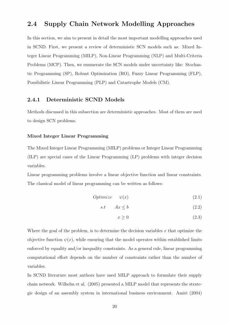
Linear programming problems involve a linear objective function and linear constraints.
The classical model of linear programming can be written as follows:
Optimize ψ(x) (2.1)
s.t Ax ≤ b (2.2)
x ≥ 0 (2.3)
Where the goal of the problem, is to determine the decision variables x that optimize the
objective function ψ(x), while ensuring that the model operates within established limits
enforced by equality and/or inequality constraints. As a general rule, linear programming
computational effort depends on the number of constraints rather than the number of
variables.
In SCND literature most authors have used MILP approach to formulate their supply
chain network. Wilhelm et al. (2005) presented a MILP model that represents the strate-
gic design of an assembly system in international business environment. Amiri (2004)
20
developed a mixed integer programming model to formulate a supply chain system prob-
lem. He designed a distribution network problem in a supply chain system that involves
locating production plants and distribution warehouses, and tried to determine the best
strategy for distributing products from plants to warehouses and from warehouses to cus-
tomers. Keskin and Ulster (2007) considered a multi-product production/distribution
system design problem. They used a mixed-integer programming approach to formulate
their problem.
Pirkul and Jayaraman (1997) proposed a mixed integer programming formulation for
multi-commodity, multi-plant, distribution system design problems. The objective is
minimize the total operating costs of the distribution network, such that all customer
demands are satisfied. Authors presented an efficient heuristic based on Lagrangian re-
laxation method, to solve the problem.
Canel and Khumawala (1997) proposed an efficient branch and bound procedure for solv-
ing the uncapacitated multi-period international facility location problem. A heuristic ap-
proach based on simulated annealing and Lagrangean relaxation was developed by Syam
(2002) for a multi-source, multi-product, multi-location framework. Jayaraman and Ross
(2003) proposed a heuristic approach based on simulated annealing for the designing
of distribution network and management in supply chain environment. Jayaraman and
Ross (2001) used simulated annealing methodology to solve a model of distribution supply
chain. Brown et al. (1987) presented a MIP multi commodity model that determines the
opening/closing of plants, the commodities produced at each plant and delivered to each
customer, and the assignment of equipment to plants. Variable production and shipping
costs, fixed costs of equipment assignment and fixed costs of plant operations were in-
cluded in the objective function.
Eskigun et al. (2005) presented a large-scale network design model for the outbound
supply chain of an automotive company. The most important characteristics mentioned
in the paper are considering lead times and choice of transportation mode. To solve this
large-scale design model, a Lagrangian heuristic is presented. The algorithm gives excel-
lent solution quality in modest computational time. Amiri (2006), Eskigun et al. (2005),
Hinojosa et al. (2008), Santoso et al. (2005), Pirkul and Jayaraman (1998), Miranda
and Garrido (2004), Sourirajan (2007), Lu and Bostel (2007) used explicitly this method
21

to solve their models. The interested reader is referred to some important reviews where
MILP are deployed in SCND problems: Tushaus and Wittmann (1998), Shu et al. (2005),
Melachrinoudis and Min (2007), Melo et al. (2006).
Non-Linear Programming
Non-linear programming problems involve either the objective function or constraints, or
both the objective function and constraints are non-linear.
Lababidi et al. (2004) developed a deterministic mixed integer non-linear programming
model to optimize the supply chain of a petrochemical company. Non-linear MIP model
presented by Cohen et al. (1989) considered the operation of a network of suppliers,
producers and markets. Min et al. (2005) presented a non-linear integer program for
solving the multi-echelon, multi commodity closed loop network design problem involving
product returns. Also, Chen and Lee (2004) proposed a multi-objective mixed integer
non-linear programming model which considers uncertainty for demands and prices, and
models according to the production, transport, sales and inventory planning stages.
Cohen et al. (1989) presented the main features that differentiate an international supply
chain model from a single-country model. The most important characteristics mentioned
in the paper are the necessity of treating multinational firms as global systems to obtain
economies of scale in order to reduce costs. A heuristic method that initially fixes the
transfer prices and allocated overhead variables, was presented.
To solve this NLP, two most popular methods, reduced gradient methods and successive
quadratic programming methods, were applied.
Multi-Criteria Problems
In real-world SCND problems, companies like to pursue more than one target or consider
more than one factor or measure. Such a desire transforms the decision making problem to
a multi-objective decision making (MODM) problem or a multi-attribute decision making
(MADM) problem. These groups of problems all come together in one category, named
multi-criteria decision making (MCDM) problems (see Figure 2.2). Furthermore, as the
bi-objective problems have become of particular consideration, they investigated them
separately from other k-objective ones. Figure 2.2 illustrates Farahani et al. (2010) clas-
22

sification of multi-criteria problems and some important papers of each problems group.
The optimization focuses in traditional SCM problems are maximizing profit or mini-
Figure 2.2: Multi-criteria problems
mizing costs as a single objective (Tsiakis et al. (2001), Santoso et al. (2005), Elhedhli
and Gzara (2008)). Nevertheless, other important criteria such as environmental criteria,
customer response time, social criteria, economic criteria should be taken into account.
- Multi-objective programming models:
In this subsection, we evaluate that part of SCND literature in which there are more
than two objectives. We call them multi-objective integer programming problems with
k-objectives (Ozlen and Azizoglu (2009)). The k-objective problem is defined as:
Optimize ψ1(x) (2.4)
Optimize ψ2(x) (2.5)
... (2.6)
Optimize ψk(x) (2.7)
s.t x ∈ X (2.8)
where the objectives are defined as ψ1(x) =n∑
j=1
c1jxj, ψ2(x) =n∑
j=1
c2jxj and ψk(x) =
n∑
j=1
ckjxj; cij is integer for all i ∈ {1, 2, · · · , k} and j ∈ {1, 2, · · · , n}. X is the set of feasi-
ble solutions in which xj ≥ 0 and integer for all j ∈ {1, 2, · · · , n}.
23

Several criteria for SCND have been appeared in literature. Alcada-Almeida et al. (2009)
proposed a multi-objective programming approach to identify locations and capacities of
hazardous material incineration facilities and balance the society, economic, and envi-
ronmental impacts. Customer response time was integrated in the distribution network
design by (Erol and Ferrell (2004), De Toni and Tonchia (2001)). Azaron et al. (2008)
used the goal attainment technique to optimize total cost, total cost variance, and fi-
nancial risk cost of a three echelon supply chain. Mincirardi et al. (2002) proposed a
multi-objective programming model to analyse solid waste management.
Paksoy et al. (2010) considered the green impact on a close-looped supply chain network
and tried to prevent more CO2 gas emissions and encourage customers to use recyclable
products via giving a small profit. They presented different transportation choices be-
tween echelons according to CO2 emissions. They also considered recyclable ratio of raw
material. Many network facility location problems utilize multi-objective optimization
concepts. Cantarella and Vitetta (2006) introduced an urban network layout and link
capacity through a multi-objective Road Network Design Problem. Pati et al. (2008)
proposed a multi-objective model for a paper recycling network system in determining
the facility location, route and flow of different varieties of recyclable waste paper in a
multi-item, multi-echelon and multi-facility environment. Selim and Ozkarahan (2006)
presented a supply chain distribution network design model that utilizes maximal cov-
ering approach in the reporting of the service level and with multiple capacity levels,
through a fuzzy multi-objective model.
Altiparmak et al. (2006) proposed a Genetic Algorithm , for designing a four-echelon
supply chain (suppliers, plants, warehouses and customers). It has three objectives to be
minimised. The first one is the cost that includes the fixed costs of operating and opening
plants and warehouses plus the cost of supplying raw materials and delivering products.
The second one is the total customer demand that can be delivered within the orders due
date. The third one is capacity utilisation for plants and warehouses.
Papers involving an integrated design of supply chain networks under uncertainty and con-
sidering several objectives is significantly smaller in number (Sabri and Beamon (2000),
Chen et al. (2008), Guillen et al. (2005). The Bi-objective integer programming prob-
lem is a special case of the multi-objective integer programming problem with only two
24

objectives Ozlen and Azizoglu (2009). Fernandez et al. (2007) presented a bi-objective
supply chain design and facility location problem of supermarkets on the plane in which
the main objective was to maximize the profit obtained by the chain, and the secondary
objective was to minimize the difference between market shares before and after entering
a new facility.
For SCND, the main criteria used were costs, price, operating service, quality, distance,
ease of access, etc. Nowadays, with changing supply chain network these criteria are not
sufficient. The set of criteria should be expanded to take into account new dimensions
and represent the ability to deal with social, environmental and economic criteria in sus-
tainable context.
- Multi-attribute problems:
There are many techniques which are used to tackle the MADM problems. The most
used ones are as follows: Analytic Network Process (ANP) (Tuzkaya et al. (2008),
Analytic Hierarchical Process (AHP) (Saaty (1980)), elimination and choice express-
ing reality (ELECTRE) (Barda et al. (1990)), Multi-Attribute Utility Theory (MAUT)
(Canbolat et al (2007)), Technique for Order Preference by Similarity to Ideal Solution
(TOPSIS) (Hwang and Yoon (1981)), Stochastic Multi-criteria Acceptability Analysis
(SMAA) (Lahdelma et al. (2002)) are utilized for solving location problems (Farahani et
al. (2010)).
One analytical approach often suggested for solving such a complex multi-criteria prob-
lem is the Analytic Hierarchy Process. The Analytic Hierarchy Process (AHP) provides a
framework to cope with multiple criteria situations, involving intuitive, rational, qualita-
tive, and quantitative aspects (Khurrum et al. (2002)). We present some of the literature
where AHP multi-attribute decision making method is used to solve location problems.
Higgs (2006) presented a waste management problem where Geographical Information
Systems (GIS) have been combined with multi-criteria evaluation techniques to take into
account the role of public in the decision making process. Tuzkaya et al. (2008) included
qualitative and quantitative criteria (benefits, opportunities, costs and risks), to assess
and select undesirable facility locations. Aras et al. (2004) employed Analytic Hierarchi-
cal Process in wind observation station location problem, and a considerable number of
criteria were taken into consideration.
25

In all these works, existing AHP approaches were applied for a very small number of
location alternatives and logistic actors are not considered in the selection criteria. To
the best of our knowledge, no comprehensive supply chain design approach, dealing with
all sustainable criteria, using GIS, has been proposed yet.
Models discussed above have several drawbacks, the most important being their deter-
ministic nature. However, in SCD problems, there are several uncertainties that should be
taken into account. Generally, in SCND problems we are not dealing only with numbers
and mathematical findings but many decisions are based on human judgement. In ad-
dition, existing multi-attribute approaches are applied for facility location problems and
logistic actors are not considered in the selection criteria. However, integrating multi-
criteria approaches with MILP problem can be an important development in supply chain
network design.
2.4.2 SCND Models Under Uncertainty
In this section, we present the most used uncertainty approaches to model SCND problems
under uncertainty, such as: stochastic approach, possibilistic approach, fuzzy approach
and the robust approach (Figure 2.3).
The future business environment where a supply chain network operates is generally
unknown and critical parameters such as customer demands, prices, and capacities are
uncertain.
Uncertainty implies that, in certain situations, a person does not dispose about informa-
tion which qualitatively is appropriate to describe, prescribe or predict deterministically
and numerically a system, its behaviour or other characteristic (Zimmermann (2001)).
However, informations are indispensable in supply chain design, in order to make ap-
propriate strategic decisions. Decision support systems provide decision makers with
useful informations to guide their thoughts and actions. Sufficient informations enable
the decision-makers to achieve the supply chain objectives through better and effective
decisions and actions. However, for many reasons these informations may be incomplete
due to many causes of uncertainty: lack of information, abundance of information, ap-
proximation, ambiguity, conflicting evidence and belief.
26

To model these uncertainties, we can find in literature numerous uncertainty approaches,
such as: probability theories (Shapiro (2003)), evidence theory (Shafer (1990)), possibility
theory (Zadeh (1965)), fuzzy set theory (Zadeh (1965)), rough set theory (Pawlak (1985)),
convex modelling (Ben-Haim and Elishakoff (1990)), etc. The most used to model supply
chain network under uncertainty is stochastic approach, where parameters are considered
as random variables with known probability distributions. The joint-events associated to
the possible values of the random variables can be considered as plausible future scenarios,
and each of these scenarios has a probability of occurrence. (Shapiro (2008), Santoso et
al. (2005), Vila et al. (2007)). A review of recent robust supply chain networks design is
found in Klibi et al. (2010). Several authors have discussed robustness in a supply chain
context (Rosenblatt and Lee (1987)), Gutierrez et al. (1996), Dong (2006), Snyder and
Daskin (2006)).
Figure 2.3 shows the most popular mathematical approaches considered by the researchers
Figure 2.3: Uncertainty Modelling Methods
for designing SCN. many papers are proposed and they are summarized in Table 2.8 and
Table 2.9. Notations used in Table 2.8 and Table 2.9 are: Average Scenario (AS), Models
based on Scenarios (MS), Two Stage Stochastic Programs (TSSP), Multi Stage Stochas-
tic Programs (MSSP), Catastroph Models (CM), Robust Optimisation (RO), Fuzzy Sets
Theory (FST), Possibilistic Programming (PP).
27

Stochastic Programming
We begin by abstracting the statement of a LP model with random parameters. Problem
(2.1)-(2.3) can be presented as follows:
Optimize ψ(x) (2.9)
s.t A(ξ)x ≤ b(ξ) (2.10)
x ≥ 0 (2.11)
Where A(ξ) and b(ξ) denote, respectively, the random coefficients matrix and right-hand-
side vector, and decision x corresponds to a setting of all the decision variables. ξ denotes
a random vector varying over a set Φ ∈ ℜk. If we model the random parameters as dis-
crete scenarios, the model (2.9)-(2.11) can be transformed into deterministic equivalent
which is an ordinary linear programming. The deterministic equivalent of the model (2.9)-
(2.11) can be introduced in various ways. Depending on how the random parameters are
modelled and whether a risk measure is included in the objective function, the resulting
deterministic equivalent model will be the two-stage stochastic programming, multi-stage
stochastic programming, and robust optimization.
In order to transform the SCN models with random parameters (2.9)-(2.11) into a deter-
ministic equivalent model, the random data should be modelled as discrete scenarios. In
SCND problems, random data can be modelled as a random variable with a stationary
distribution, or as a non-stationary and dynamic data process. In stationary distribution,
the random data are represented as a number of scenarios with known probabilities. The
origin of scenarios can come from known discrete distributions, can be obtained from the
discretization of a continuous known distribution, or they can result from a preliminary
analysis of the problem with probabilities of their occurrence that may reflect an ad hoc
belief of the problem or a subjective opinion of an expert (Dupacova (1996), Miller and
Rice (1983)). This approach for random data representation in stochastic models is illus-
trated in Figure 2.4.
In two-stage stochastic programs, the structure of the tree encloses the first and second
stage phases, as shown in Figure 2.4. The beginning of the tree is represented by a single
node of the first stage since states of the world during the first stage are known with
certainty. The second stage is represented by many nodes. This means that the scenario
28

tree is a set of individual scenarios s which occur with probabilities ps. In dynamic data
S1�
S2�
S3�
S4�
S5�
Stage�2�Stage�1�
Figure 2.4: A scenario tree in two stage stochastic programming models
�
S1�
S2�
�
Stage�2�Stage�1�
S3�
S4�
S5�
S6�
S7�
S8�
S9�
Stage�3�
Figure 2.5: A scenario tree in multi-stage stochastic programming models
process, the random data are characterized by cycles or temporal patterns, they should be
modelled as dynamic stochastic data. A representative scenario tree corresponding to the
multi-stage stochastic programming formulation (Figure 2.5) can be visualised as a tree
starting similarly with the previous case with a single node at first stage and branches
into a finite number of nodes at second stage. This branching continues for all stages of
the problem until last stage.
- Multi-stage stochastic programming:
The stochastic programming models that we have discussed so far, are static in the sense
29

that we make a decision at one point in time, while accounting for possible recourse ac-
tions after all uncertainties have been resolved. There are many situations where one
is faced with problems where decisions should be made sequentially at certain periods
of time based on information available at each time period. Such multi-stage stochastic
programming problems can be viewed as an extension of two-stage programming to a
multi-stage setting. Guan and Philpott (2009) presented an application of multi-stage
stochastic programming to a production planning problem for a leading company in the
New Zealand dairy industry, taking into account uncertain milk supply, price demand
curves and contracting. Goh et al. (2007) constructed a stochastic model of the multi-
stage global supply chain network problem, incorporating a set of related risks, namely,
supply, demand, exchange, and disruption (Shapiro and Philpott (2007)).
The equivalent deterministic models of the Multi-stage stochastic programming models
are very large in scale due to the problem structure and the size of the problem increase
as a quadratic function of the number of scenarios. To solve these models, many algo-
rithms have been presented such as the augmented Lagrangian decomposition method
(Ruszczynski (1989)) and the decomposition methods (Liu and Sun (2004)).
- Two-stage stochastic programming:
In two-stage stochastic programming, we assume that the random data has a stationary
probability distribution during the time. The decision variables are explicitly classified
according to whether they are implemented, before or after a scenario of the random data
is observed. In other words, we have a set of decisions to be taken without full information
on the random parameters. These decisions are called first-stage decisions. Later, full
information is received on scenarios of the random vector. Then, second-stage actions are
taken under the full insight on the random data. These second-stage decisions allow us to
model a response to each of the observed scenarios of the random variable. In general, this
response will also depend upon the first-stage decisions. The objective of the two-stage
stochastic model would be to minimize the first-stage cost in addition to the expected
second-stage cost for all scenarios of random parameters.
We define the two-stage stochastic linear programming corresponding to model (2.9)-
(2.11), (Shapiro (2008), Santoso et al. (2007)) as follows:
30
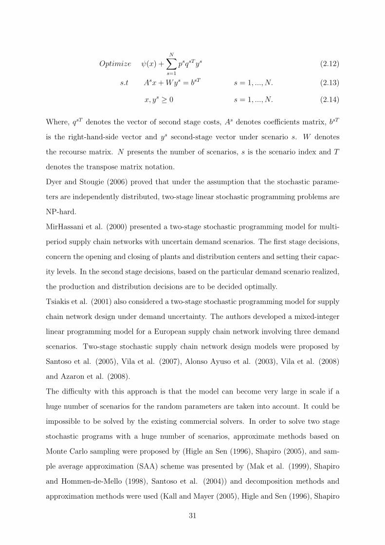
Optimize ψ(x) +N∑
s=1
psqsTys (2.12)
s.t Asx+Wys = bsT s = 1, ..., N. (2.13)
x, ys ≥ 0 s = 1, ..., N. (2.14)
Where, qsT denotes the vector of second stage costs, As denotes coefficients matrix, bsT
is the right-hand-side vector and ys second-stage vector under scenario s. W denotes
the recourse matrix. N presents the number of scenarios, s is the scenario index and T
denotes the transpose matrix notation.
Dyer and Stougie (2006) proved that under the assumption that the stochastic parame-
ters are independently distributed, two-stage linear stochastic programming problems are
NP-hard.
MirHassani et al. (2000) presented a two-stage stochastic programming model for multi-
period supply chain networks with uncertain demand scenarios. The first stage decisions,
concern the opening and closing of plants and distribution centers and setting their capac-
ity levels. In the second stage decisions, based on the particular demand scenario realized,
the production and distribution decisions are to be decided optimally.
Tsiakis et al. (2001) also considered a two-stage stochastic programming model for supply
chain network design under demand uncertainty. The authors developed a mixed-integer
linear programming model for a European supply chain network involving three demand
scenarios. Two-stage stochastic supply chain network design models were proposed by
Santoso et al. (2005), Vila et al. (2007), Alonso Ayuso et al. (2003), Vila et al. (2008)
and Azaron et al. (2008).
The difficulty with this approach is that the model can become very large in scale if a
huge number of scenarios for the random parameters are taken into account. It could be
impossible to be solved by the existing commercial solvers. In order to solve two stage
stochastic programs with a huge number of scenarios, approximate methods based on
Monte Carlo sampling were proposed by (Higle an Sen (1996), Shapiro (2005), and sam-
ple average approximation (SAA) scheme was presented by (Mak et al. (1999), Shapiro
and Hommen-de-Mello (1998), Santoso et al. (2004)) and decomposition methods and
approximation methods were used (Kall and Mayer (2005), Higle and Sen (1996), Shapiro
31
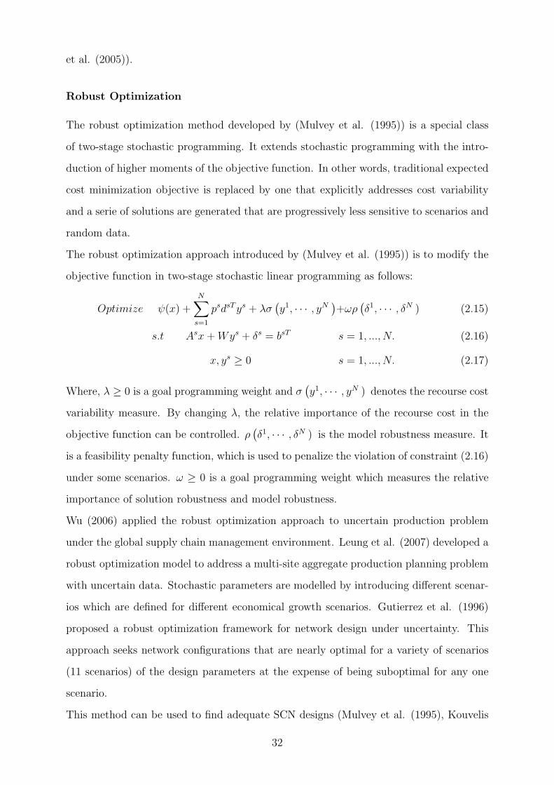
et al. (2005)).
Robust Optimization
The robust optimization method developed by (Mulvey et al. (1995)) is a special class
of two-stage stochastic programming. It extends stochastic programming with the intro-
duction of higher moments of the objective function. In other words, traditional expected
cost minimization objective is replaced by one that explicitly addresses cost variability
and a serie of solutions are generated that are progressively less sensitive to scenarios and
random data.
The robust optimization approach introduced by (Mulvey et al. (1995)) is to modify the
objective function in two-stage stochastic linear programming as follows:
Optimize ψ(x) +N∑
s=1
psdsTys + λσ(
y1, · · · , yN)
+ωρ(
δ1, · · · , δN ) (2.15)
s.t Asx+Wys + δs = bsT s = 1, ..., N. (2.16)
x, ys ≥ 0 s = 1, ..., N. (2.17)
Where, λ ≥ 0 is a goal programming weight and σ(
y1, · · · , yN ) denotes the recourse cost
variability measure. By changing λ, the relative importance of the recourse cost in the
objective function can be controlled. ρ(
δ1, · · · , δN ) is the model robustness measure. It
is a feasibility penalty function, which is used to penalize the violation of constraint (2.16)
under some scenarios. ω ≥ 0 is a goal programming weight which measures the relative
importance of solution robustness and model robustness.
Wu (2006) applied the robust optimization approach to uncertain production problem
under the global supply chain management environment. Leung et al. (2007) developed a
robust optimization model to address a multi-site aggregate production planning problem
with uncertain data. Stochastic parameters are modelled by introducing different scenar-
ios which are defined for different economical growth scenarios. Gutierrez et al. (1996)
proposed a robust optimization framework for network design under uncertainty. This
approach seeks network configurations that are nearly optimal for a variety of scenarios
(11 scenarios) of the design parameters at the expense of being suboptimal for any one
scenario.
This method can be used to find adequate SCN designs (Mulvey et al. (1995), Kouvelis
32

and Yu (1997)). It can be used with min-max regret criterion (Mulvey et al. (1995)), or
the minimization of the maximum cost and mean-variance. Mean-variance measure has
been presented in many works, namely stochastic aggregate production planning (Leung
and Wu (2004), Leung et al. (2007)), stochastic logistic problems (Yu and Li (2000)).
Robust optimization has been applied to different versions of the facility location problem
under uncertainty (Snyder and Daskin (2006), Yu and Li (2000), Gutierrez et al. (1996),
Takriti and Ahmed (2004)).
A major difficulty with this approach is the same one as two-stage stochastic program-
ming that the model can become very large in scale if a huge number of scenarios for
the random parameters are taken into account, making it impossible to be solved by the
existing commercial solvers.
The small size robust optimization models can be solved by the Cplex quadratic pro-
gramming solver. In order to solve the large size ones with large number of scenarios,
decomposition methods and approximations methods can be used (Takriti and Ahmed
(2004)).
Fuzzy Linear Programming
In SCND problems, the conventional approaches tend to be less effective in dealing with
the imprecision or uncertainty nature of the data. There has been an increasing interest
for fuzzy sets to be used for the SCDN in the recent years. The fuzzy mathematical
programming in the first category was initially developed by Bellman and Zadeh (1970).
It treats decision-making problem under fuzzy goals and constraints. The fuzzy goals
and constraints represent the flexibility of the target values of objective functions and the
elasticity of constraints.
We assume that the decision maker can establish an aspiration level, z, for the value of
the objective function he or she wants to achieve and that each of constraints is modelled
as a fuzzy set. The equivalent fuzzy linear programming of the LP (2.1)-(2.3) is (Bellman
and Zadeh (1970)):
33

Find x such that
z = ψ(x) (2.18)
s.t Ax ≤ b (2.19)
x ≥ 0 (2.20)
where x is the vector of decision variables; A and b are fuzzy quantities; operations of
addition and multiplication by a real number of fuzzy quantities are defined by Zadeh’s
extension principle; the objective function z, is to be maximized in the sense of a given
problem.
Linear programming problems with fuzzy parameters are formulated by fuzzy functions.
The ambiguity considered here is not randomness, but fuzziness which is associated with
the lack of a sharp transition from membership to non-membership. Parameters on con-
straint, relationship between constraints or objective functions and objective functions
are given by fuzzy numbers.
Fuzzy linear programming problem with fuzzy numbers can be regarded as a model of
decision problems where human estimation is influential. The model helps in determining
the optimal number and site locations of fire stations at an international airport. Several
distinct methods are frequently mentioned for representing uncertainty. For example, the
fuzzy-based approach (Giannoccaro et al. (2003), Liu and Sahinidis (1997), Petrovic et
al. (1998), (1999)), where in the forecast parameters are considered as fuzzy numbers
with accompanied membership functions.
Possibilistic Linear Programming
Zadeh (1978) presented the theory of possibility, which is related to the theory of fuzzy
sets by defining the concept of possibility distribution as a fuzzy restriction. After pio-
neering work of Zadeh, possibility theory has found gradual acceptance in the literature.
Several research efforts have concentrated on possibilistic linear programming (Buckley
(1988), Buckley (1989), Hsu and Wang (2001)). In this section, we consider the following
34

possibilistic linear programming problem:
Optimize ψ(x) (2.21)
s.t Ax ≤ b (2.22)
x ≥ 0 (2.23)
Where, A is a matrix represented by a possibility distribution and b is a possibilistic vari-
able restricted by a possibility distribution. Wang and Shu (2010) suggested a possibilistic
decision model to determine the supply chain configuration and inventory policies for new
products with unreliable or unavailable statistical data. Fuzzy sets were used to model
uncertain and flexible supply chain parameters such as total supply chain cost, demand,
service time, lead and response time. Authors presented a case study of computer assem-
bly company to evaluate the performance of the entire supply chain.
Wang and Liang (2005) presented a possibilistic linear programming (PLP) approach for
solving the multi-product aggregate production planning problem with imprecise param-
eters : customer demands, operating costs and capacities. They used LINDO computer
software to solve the model. Peidro et al. (2009) proposed a fuzzy mathematical pro-
gramming model for supply chain planning which considers supply, demand and process
uncertainties. The model has been formulated as a fuzzy mixed integer linear program-
ming model where data are unknown and modelled by triangular fuzzy numbers. They
tested the proposed PLP on an automotive supply chain network involving: 44 suppliers,
one seat manufacturer, one seat assembly plant and an Automobile Assembly Plant. To
solve the MILP model they used the CPLEX 9.0 solver. Petrovic et al. (1999) considered
a production supply chain with all facilities in a serial connection. The supply chain
includes inventories and production facilities between them. Authors assumed customer
demand and supply deliveries as uncertain parameters, and proposed small computational
examples showing that uncertain customer demands and uncertain supply deliveries along
the supply chain have great impact on supply chain behaviour.
Torabi and Hassini (2008) considered a supply chain master planning model consisting of
multiple suppliers, one manufacturer and multiple distribution centers. They proposed
a new multi-objective PLP model for integrating procurement, production and distri-
bution planning with imprecise nature of many parameters such as demands, cost/time
35

coefficients and capacity levels. To validate their model they advised an industrial case
involves 4 suppliers, one manufacturer and 3 distribution centers located in different cus-
tomer zones. They solved the instances using OSL solver from IBM.
There are different approaches to solve probabilistic SCND problems. To convert the
original model into an equivalent auxiliary crisp model, efficient possibilistic methods
are proposed by Jimenez et al. (2007) and Parra et al. (2005). To find the final pre-
ferred compromise solution, the reader can refer to recently proposed fuzzy methods of
Torabi and Hassini (2008) and Selim and Ozkarahan (2008). As evident from the above
discussion, the existing possibilistic linear programming approaches for supply chain de-
sign under uncertainty are suited for very small size problems and a limited number of
fuzzy parameters. In addition, the majority of these papers are theoretical (Kabak et al.
(2011)).
Models Based on Scenarios
An other alternative is to solve the deterministic model for a set of representative scenarios,
and to evaluate the solution obtained. The difficulty with this approach is to determine
which among solutions found is the best. Many methods have been used to evaluate and
select solutions obtained such as Monte-Carlo sensitivity analysis (Saltelli et al. (2004),
Ridlehoover (2004)), screening procedure using many filtering criteria such as Pareto
optimality and mean-variance. Good examples of how this approach works, are found in
Vidal and Goetschalchx (2000), Mohamed (1999).
Average scenario is an approach often used to solve supply chain network problems under
uncertainty, by elaborating an average scenario, and then solve the resulting deterministic
model.
The solution obtained is not necessary optimal. Solutions may be very bad or even
infeasible under specific scenarios (Sen and Higle (1999)).
Catastrophe Models
Catastrophe models used to estimate the location, severity and frequency of potential
future natural disaster. They are usually based on catastrophe arrival process, and they
provide a compromise between economic loss and the probability that certain level of
36

loss will be exceeded on an annual basis (Haimes (2004), Grossi and Kunreuther (2005),
Banks (2006)). Qualitative SC disruptions risk identification and assessment approaches
were proposed by Kleindorfer and Saad (2005) and Manuj and Mentzer (2008).
To conclude this discussion of SCND models under uncertainty, note that the most
used approach in SCND under uncertainty are stochastic linear programming approach
and robust models. The most important problem with these approaches is that the
model can become very large in scale for a small number of scenarios for the random
parameters are taken into account. It could be impossible to be solved by the existing
commercial solvers. Only few models based on the possibilty and fuzzy sets on SCND
problems are proposed in literature (Sule (2001), Torabi and Hassini (2008), Wang and
Shu (2007)). Other approaches such as evidence theory, rough set theory (Pawlak (1985))
and convex modelling (Ben-Haim and Elishakoff (1990)), etc. were used by authors to
model uncertainty.
2.4.3 Resolution Methods
As we discussed before, various approaches such as Branch-and-Bound, Bender decompo-
sition and Lagrangian relaxation were proposed for solving the SCND problem. However,
not all of these methods are regarded as feasible when the size of the system increases.
For small size network systems, exact methods can be used to solve the SCND problems.
For larger systems, exact methods fail because the size of the solution space increases
exponentially with the number of constraints and variables in the network. As a result,
the computation time of exact methods becomes impractical. In these cases, heuristic or
meta-heuristic methods can be used to produce near optimal solutions in a reasonable
computation time. Table 2.10 and Table 2.11 classify the literature according to most
important resolution methods used in solving SCND problems.
2.5 Concluding Remarks
In this chapter, we have described a review of mathematical programming models and
resolution methods for SCND. We have proposed a classification based on the analysis of
37

three aspects: supply chain network structure, decision level and supply chain modelling
approaches.
Conclusions drawn from this chapter affirm that: (i) papers integrating multiple periods,
multiple products, multiple criteria, multiple transportation modes, multiple objective
and uncertainty in SCND context are still scarce, (ii) the most widely used modelling
approach is mixed integer linear programming, where the use of heuristic algorithms and
meta-heuristics to solve the approach stands out, (iii) more proposed models validated by
small numerical examples are presented than case studies applied to real supply chains.
The design of a multi-criteria supply chain network to respect the environmental, social,
legislative, and economical aspects and to satisfy customer demands, is presented in the
next chapter.
38

Table 2.8: Supply chain design under uncertainty (Part 1)
Authors AS MS TSSP MSSP CM RO FST PP
Eppen et al. (1989) X
Mulvey et al. (1995) X X
Gutierrez et al. (1996) X
Huchzermeier and Cohen (1996) X
Kouvelis and Yu (1997) X
Bok et al. (1998) X
Kurksalan and Sural (1999) X
Mohamed (1999) X
Sen and Higle (1999) X
Vidal and Goetschalckx (2000) X
Yu and Li (2000) X
Sule (2001) X
Tsiakis et al. (2001) X
Lowe et al. (2002) X
Ahmed and Sahinidis (2003) X
Ruszczynski and shapiro (2003) X
Shapiro (2003) X
Kahraman et al. (2003) X
Saltelli at al, (2004) X
Ridlehoover (2004) X
Haimes (2004) X
Christopher and lee (2004) X
Santoso et al. (2005) X
Grossi and Kunreuther (2005) X
39

Table 2.9: Supply chain design under uncertainty (Part 2)
Authors AS DMS TSSP MSSP CM RO FST PP
Kleindorfer and saad (2005) X
Sheffi (2005) X
Snyder and Daskin (2006) X
Chen and Lee (2006) X
Banks (2006) X
Shapiro (2007) X X
Vila et al. (2007) X
Wang and Shu (2007) X
Torabi and Hassini (2007) X
Matos (2007) X
Vila et al. (2008) X
Manuj and Mentzer (2008) X
40

Table 2.10: Resolution Methods
Authors Heuristic Meta-heuristic Resolution Method
Aghezzaf (2005) X Lagrangean Relaxation
Lu and Bostel (2007) X Lagrangean Relaxation
Aliev et al. (2007) X Genetic algorithm
Amiri (2006) X Lagrangean Relaxation
Arntzen et al. (1995) X Factorization
Barahona and Jens (1998) X Decomposition techniques
Barros et al. (1998) X Relaxation heuristic
Brown and Olson (1994) X Factorization
Brown et al. (1987) X Decomposition
Canel and Khumawala (1997) X Branch and Bound
Canel and Khumawala (2001) X Branch and Bound
Cohen and Lee (1985) X A heuristic method
Cohen and Lee (1989) X Relaxation and Approximation
Cohen and Moon (1991) X Benders Decomposition
Cohen et al. (1989) X Relaxation and Approximation
Cole (1995) X Branch and Bound
Cordeau et al. (2006) X Benders Decomposition
Dogan and Goetschalckx (1999) X Valid inequalities
Eksioglu et al. (2006) X Relaxation and Approximation
Erlebacher and Meller (2000) X Relaxation and Approximation
Eskigun et al. (2005) X Lagrangean Relaxation
Geoffrion and Graves (1974) X Benders Decomposition
Geoffrion et al. (1978) X Decomposition techniques
Geoffrion et al. (1982) X Decomposition techniques
Goetschalckx et al. (2002) X Decomposition techniques
Goetschalckx et al. (1994, 1995) X Decomposition techniques
41

Table 2.11: Resolution Methods
Authors Heuristic Meta-heuristic Resolution Method
Hinojosa et al. (2000) X Lagrangean Relaxation
Hinojosa et al. (2008) X Lagrangean Relaxation
Hodder and Dincer (1986) X Relaxation and Approximation
Hwang (2002) X Genetic Algorithm
Jang et al. (2002) X Genetic Algorithm
Jayaraman and Pirkul (2001) X Lagrangean Relaxation
Jayaraman and Pirkul(2001) X Lagrangian relaxation
Jayaraman and Ross (2003) X Simulated Annealing
Jayaraman et al. (2003) X Decomposition techniques
Keskin and Ulster (2007) X Tabu Search
Ko and Evans (2007) X Genetic Algorithm
Lee and Dong (2008) X Decomposition techniques
Lieckens and Vandaele (2007) X Genetic Algorithm
Listes (2006) X L-Shaped
Ma and Davidrajuh (2005) X Genetic Algorithm
Marin and Pelegrin (1999) X Lagrangean Relaxation
Min et al. (2006) X Genetic Algorithm
Miranda and Garrido (2004) X Lagrangean Relaxation
Paquet et al. (2004) X Valid inequalities
Pirkul and Jayaraman (1998) X Lagrangean Relaxation
Romeijn et al. (2007) X Column Generation
Santoso et al. (2005) X Lagrangean Relaxation
Shu (2004) X Column Generation
Sourirajan (2007) X Lagrangean Relaxation
Vidal and Goetschalckx (1996) X Branch and Bound
42
Chapter 3
Multi-criteria Supply Chain Network
Design
3.1 Introduction
The main purpose of this chapter is to present a novel framework for multi-criteria Supply
Chain Network Design (SCND) as well as its application to real Supply Chain Network
(SCN).
This chapter deals with the design of a multi-criteria supply chain network in order to
satisfy the customer demands and to respect the environmental, social, legislative, and
economical requirements.
The methodology consists of two different steps. The first step looks for the best potential
facility locations to open in order to satisfy the different criteria: environmental, social,
and legislation aspects, using the overlay weighted and Analytic Hierarchy Process (AHP).
The second step looks for the optimal supply chain design to fulfill customer demands
and economic criteria using mixed integer linear programming model. The objective in
this step is to determine location of treatment facilities and their capacities minimizing
the sum of: opening facilities cost, products storage cost, production cost, transportation
cost, and CO2 emissions taxes. We apply our methodology to a real life application
concerning the recycling of sediment waterways, which was presented in Bouzembrak et
al. (2010).
The chapter is organized as follows. In Section 3.2, we describe the problem in more
43

detail. In Section 3.3, we discuss our proposed methodology. In Section 3.4, we present
the real case. The experimental study is discussed in Section 3.5. Finally, Section 3.6
contains some concluding remarks.
3.2 Problem description
Before presenting the methodology, we will briefly introduce a multi-criteria, multi-level,
single product, single period and multi-modal supply chain network problem (see Table
3.1). Figure 3.1 depicts a supply chain network that includes different transportation
modes: roads, railways and waterways. The network has four levels: suppliers, storage
depots, production plants and customers. In addition to different types of transportation
modes, the possible flows of material are shown in the Figure 3.1. Multi-criteria supply
Roads : Railways : Waterways :
Suppliers Storage
depots
Production
plants Customers
Figure 3.1: Supply chain network
Table 3.1: Problem description
Criteria Level Product Period Modalily
Single X X
Multiple X X X
chain network design problems are complex and, like most real world problems depend on a
multitude of criteria and uncertain parameters. Many factors contribute to the complexity
44

of the model. The first one is the multi-criteria aspect. For example, problems involving
many criteria decision are much more difficult than problems involving only one criterion
decision. The second factor is the integration of multi-modality and CO2 emissions taxes
in the model. Indeed, the majority of papers consider only one transportation mode. The
third factor is uncertainty which will be addressed in Chapter 6.
3.2.1 SCND evaluation criteria
In the section below, we aim to present in detail the most popular criteria in the literature
used for design supply chain networks.
As we explained in Chapter 2, the majority of papers, in supply chain network design lit-
erature, propose a cost minimization objective and their aim is to determine the network
configuration with the least total cost. These models do not gather several of the criteria
depicted in Figure 3.2, simultaneously.
Thus, in this thesis, we will integrate, simultaneously, four different categories of aspects
in the SCND, which are: environmental aspects, social aspects, regulation aspects and
economic aspects.
In actual business world, thinking of criteria other than economic one (like profit, cost,
revenue, etc) is becoming an important opportunity. Sustainability imposes on any de-
velopment and design, like in supply chain network design, to consider social and envi-
ronmental aspects (see Dehghanian and Mansour (2009)).
When a selection decision needs to be made, the company establishes a set of evaluation
criteria that make it possible to compare potential performance features (Masella and
Rangone (2000)). In single criterion SCND problems, the criterion has usually been cost.
However, in multi-criteria SCND problems, there is at least one other criterion to consider
which, for the nature of these problems, is in conflict with the first one. As the number of
criteria used in such problems is important, we decided to present the main criteria that
we will consider in this work, in some general categories (Figure 3.2) which are:
Environmental aspects
Environmental aspects are matters on health effects, sound and optical pollution, smells,
air or water pollution, transportation risk, natural risk, waste disposal or treatment risk,
45

• Proximity to urban areas.
• Education.
• Labor availability.
• Security.
• Resting, accommodation
• Land use.
• Pollution.
• Health effects.
• …etc
�
�
����������� ����
������
�� ����
�������������� ����
�����
�� ����
•
•
•
•
•
•
•
•
•
•
�
• Water pollution.
• Waste.
• Green house gases.
• Health effects.
• Sound pollution.
• Closeness to natural areas.
• Natural threats.
• …etc.
�
• Forbidden areas.
• Country measures.
• Community consideration.
• …etc
�
Land cost.
Transportation cost.
Installation cost.
Production cost.
Storage cost
Resource accessibility
Business climate.
Closeness to customers,
suppliers and resources.
Infrastructure
…etc.
Figure 3.2: Sustainable supply chain network criteria
the protection of natural area , etc.).
Social aspects
In this category, we can find cultural and social aspects: education, labour availability,
job opportunities, security, land use, natural threats, pollution, resting, accommodation,
infrastructure and any other factors which represent this category.
Political and regulations aspects
Political matters and regulations include community consideration, country measures, and
government regulations.
Economical criteria
- Cost: There are different types of cost. These types can be divided into fixed and
variable. Fixed cost includes installation and opening cost, along with investment. Vari-
able cost can be transportation, inventory, production, services, distribution, logistics,
waste disposal, maintenance and environmental cost. Generally, transportation cost is
46

the highest and installation cost is the second one. Several problems have used a total
cost criterion which contains all costs under one objective. Other criteria like currency
value, business climate, access to public facilities like airports, roads or railways infras-
tructure, could be taken into account.
- Profit: Some problems are interested in the net profit, difference between benefits and
costs, or other outcomes of the capital they invested in their facility location decision
making. We assembled these criteria under the profit category.
- Coverage: Most of location problems, are about coverage by distance, time, amount or
even coverage deviation. Although many problems use distance and population coverage
as their criteria, time is well considered in some problems.
For a deeper understanding of criteria cited above, the reader can refer to Farahani et al.
(2010), Alcada-Almeida et al. (2009), De Toni and Tonchia (2001), Azaron et al. (2008),
Chen et al. (2008).
3.2.2 Multi-modality in SCND
The main four transportation modes for freight are: rail, road, water, and air. Each of
these modes has different characteristics, and any of them can be considered the best un-
der different circumstances, depending on the location, distance, pollution, type of freight,
and value of freight, among other things. The main criteria for transportation are the
type and volume of freight and the distance to be covered. Other criteria may include
speed, availability, reliability, capacity, security, and frequency of delivery (Tuzkaya and
Onut (2008)).
According to Vidal and Goetschalckx (1997), several important SC features are ignored
in the methodology for the strategic and tactical planning of global logistics systems.
One of these factors is the integration of transportation modes in the SCND. Also, as we
showed in chapter 2, the existing literature integrating transportation modes in supply
chain network design, is still scarce. Only 7% of these papers included these aspects.
Arntzen et al. (1995) developed a mixed integer linear program to solve the global supply
chain design problem at an Electronic manufacturer. They proposed supply chain prob-
lem that involves multiple products, production stages, time periods, and transportation
modes. The objective function is to minimize fixed and variable production costs, inven-
47

tory costs, and distribution expenses, including transportation, taxes, and duties.
Cordeau et al. (2006) introduced a new formulation of logistics network design problem.
Authors integrated location and capacity choices for plants and warehouses with supplier
and transportation mode selection, product range assignment and product flows.
Carlsson and Ronnqvist (2005) integrated three transportation modes in the design of
the larger Swedish forest company supply chain network. The international three possi-
ble modes of transportation are vessel, train and lorry. A detailed discussion regarding
this aspect is provided in Carlsson and Ronnqvist (2005).
The strategic supply chain network we intend to elaborate should respect criteria
elaborated above, problem constraints and answer the following questions: (i) how many
production plants should be installed? (ii) where new sites should be located? (iii) how
much goods should each production plant handle? (iv) which customers should be served
by each production site? (v) products quantities to transport throughout the supply chain
network? (vi) which transportation mode should be used?
3.3 Approach presentation
In this section, we detail the idea of the novel multi-criteria supply chain network design
methodology by explaining each step with small examples. We start by providing the
basic steps of our methodology design.
Our method, as illustrated in Figure 3.3, contains two steps. The first step is related to
the identification of the potential facility locations set and to satisfy the different criteria:
environmental, social, and legislation aspect, using Geographic Information System (GIS)
overlay weighted and AHP method. The GIS model is implemented on a Arcview 9.2 GIS
to locate elements of the potential facility set. The second step looks for the optimal supply
chain design to satisfy customer demands and economic criteria using mixed integer linear
programming model. These approaches will be presented in detail in the next chapters.
Figure 3.3 presents two steps of our methodology. Now that you have seen the basic
outline of two steps, lets delve into the methodology process in more detail.
48
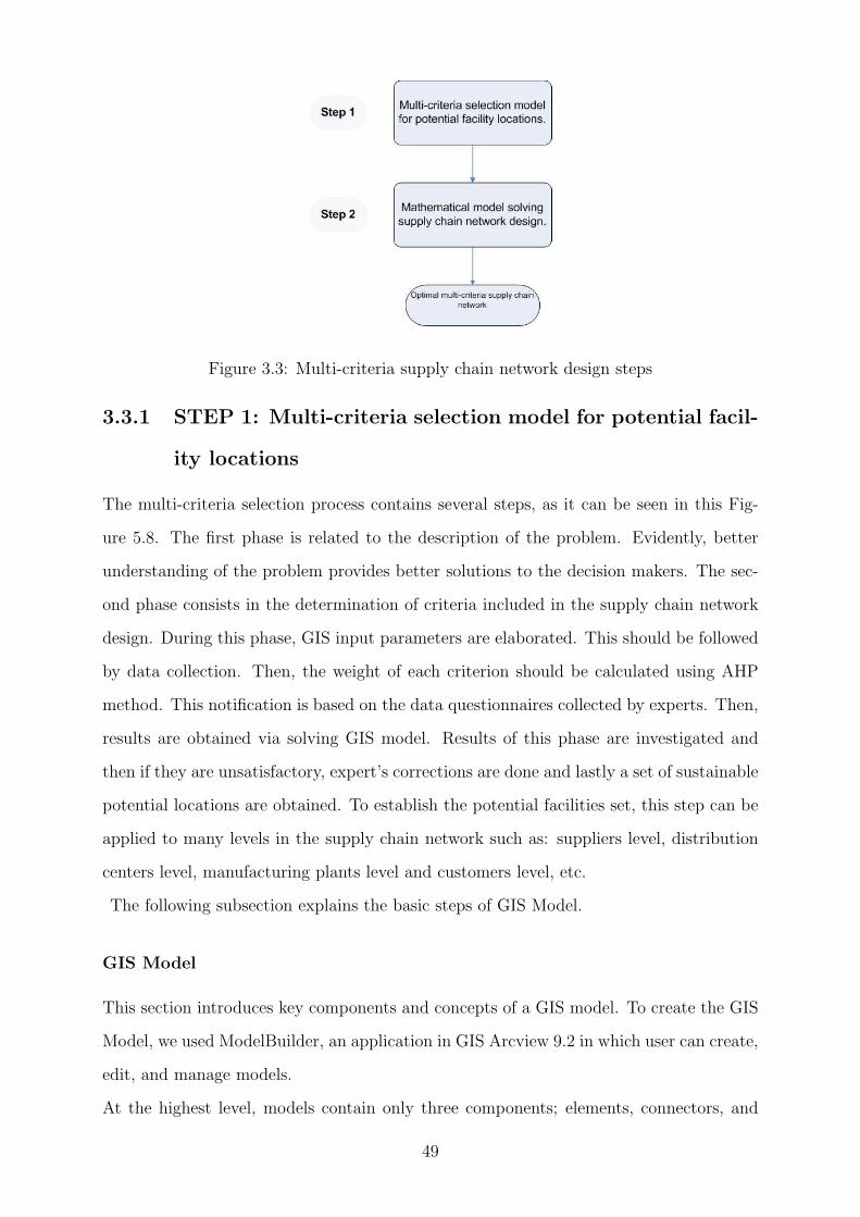
Figure 3.3: Multi-criteria supply chain network design steps
3.3.1 STEP 1: Multi-criteria selection model for potential facil-
ity locations
The multi-criteria selection process contains several steps, as it can be seen in this Fig-
ure 5.8. The first phase is related to the description of the problem. Evidently, better
understanding of the problem provides better solutions to the decision makers. The sec-
ond phase consists in the determination of criteria included in the supply chain network
design. During this phase, GIS input parameters are elaborated. This should be followed
by data collection. Then, the weight of each criterion should be calculated using AHP
method. This notification is based on the data questionnaires collected by experts. Then,
results are obtained via solving GIS model. Results of this phase are investigated and
then if they are unsatisfactory, expert’s corrections are done and lastly a set of sustainable
potential locations are obtained. To establish the potential facilities set, this step can be
applied to many levels in the supply chain network such as: suppliers level, distribution
centers level, manufacturing plants level and customers level, etc.
The following subsection explains the basic steps of GIS Model.
GIS Model
This section introduces key components and concepts of a GIS model. To create the GIS
Model, we used ModelBuilder, an application in GIS Arcview 9.2 in which user can create,
edit, and manage models.
At the highest level, models contain only three components; elements, connectors, and
49

Figure 3.4: First step phases
text labels. Elements are the data and tools you work with. Connectors are lines that
connect data to tools. Text labels can be associated with the entire model, individual
elements, or individual connectors (Arcview (2010)).
As we can see on Figure 3.5, a process consists of a tool and all variables are connected
to it. Connector lines indicate the sequence of processing. In this GIS Model several
processes are chained together, C1, C2, · · · , Cn; so that the derived data from one process
becomes the input data for another process, as shown in the following diagram (Figure
3.6). A real case GIS model will be presented in section 3.4.
50

Project�
Data�Tool� Derived�
Data�
Figure 3.5: Structure of GIS process
�
�
�
�
�
�
�
�
�
�
�
�
�
���������������������������������������������������������������������������������������������������������������
�
�
�
Project�
Data�Tool�
�
Derived�
Data�C2�
Cn�Project�
Data�Tool� Derived�
Data�
Tool� Derived�
Data�
Project�
Data�Tool� Derived�
Data�C1�
Process�Process�
Process�
Process�
Figure 3.6: GIS Model
The weighted overlay process
The second method that we integrate in this step is the weighted overlay. In general, the
weighted overlay function involves the combination of different data layers. Practically,
this can involve a number of different processes depending on inputs to analyse (Arcview
(2010)).
Supply chain network design problems often require analysis of many different factors.
For instance, choosing the location of a new facility means assessing such things as land
cost, proximity to existing services, environmental aspects, legislative aspects and social
aspects. These information should be elaborated in different rasters with different value
scales: Euro, distances, degrees, and so on.
The Weighted Overlay tool lets as to take all these criteria into consideration. It reclassi-
fies values in the input rasters into a common evaluation scale of suitability or preference,
risk, or some similarly unifying scale. The input rasters are weighted by importance and
added together to produce an output raster. Steps are summarized as follows:
- A numeric evaluation scale is chosen. This may be 1 to 9, or any other scale. In this
thesis we will use the Saaty scale (Table 3.2).
51

- The cell values for each input raster in the analysis are assigned values from the evalu-
ation scale and reclassified to these values. This makes it possible to perform arithmetic
operations on rasters that originally held dissimilar types of values.
- Each input raster is weighted, or assigned a percent influence, based on its importance
to the model.
- The total influence for all rasters equals to 100 percent.
- The cell values of each input raster are multiplied by the raster’s weight.
- The resulting cell values are added together to produce the output raster.
Example:
Below, we provide illustrative example composed of two layers. The two input rasters
1 2 2 1 6 2 1 5 2
1 1 5 + 5 1 1 = 4 1 2
1 4 1 9 0 9 7 1 7
0,25 0,75
Figure 3.7: Raster Layers
above (Figure 3.7) have been reclassified to an evaluation scale of 1 to 9 (Table 3.2). Each
raster is assigned a weight. The weight of the first raster is 25% and the weight of the
second is 75%. The cell values are multiplied by their weights, then added together to
create the output raster.
Take the top middle cell as an example (2 × 0.25) = 0.5 and (6 × 0.75) = 4.5. The sum
of 0.5 and 4.5 is 5.
Determination of criteria weights using AHP
In this section, we provide a description of AHP method and give some examples in the
next section.
The AHP is a relatively simple and systematic approach that can be used by decision
makers, firstly introduced by Saaty (1980). In general, AHP consists of five main steps: hi-
erarchy construction, pairwise comparison, relative weights estimation, consistency check
and synthesizing (Saaty (1980)).
52

- Hierarchy construction: the hierarchy construction step consists of decomposing the
problem into hierarchical structural with distinctive levels which are, generally, the goal
level, criteria, and decision alternatives. The decomposition can be obtained using a
graphical representation, as shown in Figure 3.8.
- Pairwise comparison: this step involves establishing priorities at each level by com-
Figure 3.8: AHP graphical representation
paring pairwise each criteria and alternatives. Experts express the relative importance
of one criterion versus another regarding the fixed objective, and express also the rela-
tive importance of one alternative versus another regarding each criterion. Since experts’
judgements are used as a scale, the alternative ratios reflect the relative importance of
the criteria in achieving the goal.
Experts’ judgements are based on the scale of relative importance that assumes values
between 0 and 9 (Kim et al. (1999), Saaty (1980)) as presented in Table 3.2. A Basic
assumption is that if attribute A is absolutely more important than attribute B and is
rated at 9, then B must be absolutely less important than A and is valued at1
9.
53

- Relative weights estimation: this step involves calculating the relative weights of crite-
Table 3.2: Saaty Rating Scale
Weight Definition Explanation
1 Equal importance Two activities contribute equally to the objective
2 Weak Between equal and moderate
3 Moderate importance Experience and judgement slightly favor one activ-
ity over another
4 Moderate plus Between moderate and strong
5 Strong importance Experience and judgement strongly favor one ac-
tivity over another
6 Strong plus Between strong and very strong
7 Very strong or demon-
strated importance
An activity is favored very strongly over another;
its dominance demonstrated in practice
8 Very, very strong Between very strong and extreme
9 Extreme importance The evidence favoring one activity over another is
of the highest possible order of affirmation
ria; technically, this set is called an eigenvector. We prefer to use the right eigenvector
method to show how the relative weights are calculated because of its simplicity.
- Consistency check: the final step is to calculate a Consistency Ratio (CR) to check
how matrix judgements is consistent. It is checking at each level of the hierarchy. It is
calculated by:
CI =(λmax − n)
(n− 1)and CR =
CI
RI(3.1)
CR =
0.05 n = 3
0.08 n = 4
0.10 n > 4
(3.2)
Where, CI is the Consistency Index, n is the number of criteria, λmax is the largest
eigenvalue of judgements matrix, RI is the Random Index which depends on the number
of criteria n. We can find in Saaty (1980) matrix the RI value for each n. It is noted
in Saaty (2008), if CR is less than or equal to the given upper bound (3.2), matrix is of
54

sufficient consistency and the judgement is acceptable.
- Synthesizing: this step consists of determining overall rating and normalized priorities
of alternatives by aggregating the relative weights of criteria.
In Appendix A, we provide an example of AHP method, where we calculate weights, CI,
λmax and RI, so that a reader can further study the technique.
3.3.2 STEP 2: Mathematical model solving supply chain net-
work design
There is a wealth of literature and research on modelling of strategic supply chain, but
with an apparent lack of consideration of transportation mode and CO2 taxes. Hence,
in this part, we formulate a strategic supply chain network design model which includes
explicitly the carbon taxes and multi-modality.
Figure 5.9 shows the second step phases. The set of potential facilities is defined in
the first step. Expert arguments are taken to determine costs and inputs parameters.
Then, variables, costs, constraints and all input parameters are determined and then
the model is solved. In results evaluation phase, results are investigated and they are
unsatisfactory, expert corrections are done. Last, optimal multi criteria supply chain
design is represented.
Mathematical Model
Notation used for the formulation of the model is:
The objective function (3.3) minimizes the sum of the fixed facility location costs, the
transportation, storage, and CO2 emissions costs from supply points to storage depots.
The shipment, the processing, and CO2 emissions costs from storage depots to produc-
tion facilities. The transportation and CO2 emissions costs from production facilities to
customers.
Minimize ψ
ψ = OC + ω1 · [TC + SC +RC] + ω2 · EC (3.3)
Where
55

Figure 3.9: Second step phases
56

- Sets size:
I number of suppliers.
J number of storage depots.
K number of potential production plants locations.
L number of customers.
M number of transportation modes.
- Sets and indexes:
S set of suppliers, indexed by i.
D set of storage depots, indexed by j.
K set of potential production plants locations, indexed by k.
C set of customers indexed by l.
T set of transportation modes, indexed by m.
- Inputs are:
COk The fixed cost of opening production facility j (e).
Cijm The unit transportation costs of goods between supplier i and storage depot
k using transportation mode m (e/Ton).
Cjkm The unit transportation costs of product between storage depot j and produc-
tion site k using transportation mode m (e/Ton).
Cklm The unit transportation costs of product between production facility k and
customer l using transportation mode m (e/Ton).
ϑijm The distance between supplier i and storage depot k using transportation mode
m (Km).
ϑjkm The distance between storage depot j and production facility k using trans-
portation mode m (Km).
ϑklm The distance between production facility k and customer l using transportation
mode m (Km).
CTk The processing costs at production facility k (e/Ton).
CSj The storage costs at storage depot j (e/Ton).
Qk The maximum processing quantity of production facility k (Tons/Year).
57
Qj The storage capacity of storage depot j (Tons/Year).
βm The unit CO2 emission using transportation mode m (Tons/Ton.Km).
ω1 Weight of economic dimension (%).
ω2 Weight of environmental dimension (%).
γ Carbon taxes (e/Ton).
Qijm The transportation capacity between supplier i and storage depot k using
transportation mode m (Tons).
Qjkm The transportation capacity between storage depot j and production facility
k using transportation mode m (Tons).
Qklm The transportation capacity between production facility j and customer l using
transportation mode m (Tons).
Dl The demand of costumer l (Tons).
- Decision variables:
Xk =1 if production facility k is opened =0 otherwise
qijm The amount of goods shipped from the supplier i to the storage depot j using
transportation mode m.
qjkm The amount of goods shipped from the storage depot j to the production site
k using transportation mode m.
qklm The amount of goods shipped from the production site k to the customer l
using transportation mode m.
- Opening costs denoted by OC:
OC =∑
k
(COk ·Xj) (3.4)
- Transportation costs denoted by TC:
TC =
[
∑
i,j,m
Cijm · qijm +∑
j,k,m
Cjkm · qjkm +∑
k,l,m
Cklm · qklm
]
(3.5)
- Storage costs denoted by SC:
SC =∑
i,j,m
CSj · qijm (3.6)
58

- Treatment costs denoted by RC:
RC =∑
j,k,m
CTk · qjkm (3.7)
- Environmental costs denoted by EC:
The greenhouse gases include carbon dioxide CO2, nitrous oxide NOx, and carbon monox-
ide CO. Modes of transport are considered to be only the source of CO2 in our case. The
CO2 emissions of each mean of transport in the way back are integrated. The environ-
mental costs function is formulated as:
EC = γ ·
[
∑
i,j,m
ϑijm · βm · (qijm + 1) +∑
j,k,m
ϑjkm · βm · (qjkm + 1)+
∑
k,l,m
ϑklm · βm · (qklm + 1)
]
(3.8)
Subject to
Constraint (3.9) guarantees that the demand of the customers will be satisfied.
∑
k,m
qklm = Dl ∀l ∈ C (3.9)
Constraint (3.10) imposes a capacity restriction for each storage depot.
∑
i,m
qijm ≤ Qj ∀j ∈ D (3.10)
Constraint (3.11) limits the capacity of the production facilities.
∑
j,m
qjkm ≤ Qk ·Xk ∀K ∈ K (3.11)
Constraints (3.12), (3.13) enforce the flow conservation of the product.
∑
k,m
qjkm =∑
i,m
qijm ∀j ∈ D (3.12)
∑
j,m
qjkm =∑
l,m
qklm ∀k ∈ K (3.13)
Constraints (3.14), (3.15), (3.16) impose a capacity restriction of each mode of transport
throughout the network.
qijm ≤ Qijm ∀i ∈ S, ∀j ∈ D, ∀m ∈M (3.14)
59
qjkm ≤ Qjkm ∀k ∈ K, ∀j ∈ D, ∀m ∈M (3.15)
qklm ≤ Qklm ∀k ∈ K, ∀l ∈ C, ∀m ∈M (3.16)
Constraint (3.17) enforces the binary nature of the configuration decisions for the facilities.
Xk ∈ {0, 1} ∀k ∈ K (3.17)
Constraints (3.18), (3.19), (3.20) are standard integrality and non-negativity constraints.
qijm ≥ 0 ∀i ∈ S, ∀j ∈ D, ∀m ∈M (3.18)
qjkm ≥ 0 ∀k ∈ K, ∀j ∈ D, ∀m ∈M (3.19)
qklm ≥ 0 ∀k ∈ K, ∀l ∈ C, ∀m ∈M (3.20)
It is important to remark that our multi-criteria supply chain network design method
is such that two steps cooperate in designing the network. Each step may execute an
appropriate task. The first one is to determine the set of sustainable potential facilities.
The second one is to give the optimal design of the SCN.
3.4 Case study
To illustrate the concept of the two-step multi-criteria methodology that we have seen
above, we would like to present an application case to validate our methodology steps.
This study focuses on inland waterways sediments recycling in NPDC (Nord-Pas De
Calais) region in France (Bouzembrak et al. (2010)). These sediments have been stored
along waterways or in some agriculture lands, used as depots, bought by French waterways
VNF (Voies Navigable de France). However, these sediments could be polluted with zinc,
plumb, cadmium and mercury. VNF management plans to recycle waterways sediments
because of new European directive exists.
3.4.1 Supply Chain Network
Treatment process steps are as follows: sediments which come for treatment are sent to
phosphating where heavy metals are stabilized by capturing them in calcium phosphate
60

matrix and then the organic compounds are destroyed by calcination to get clean sed-
iments that can be used by customers (Novosol (2009)). In France, treated waterways
sediments can be used in the following areas: (i) brickworks, (ii) concrete facilities, (iii)
concrete stations, (iv) roads projects.
A schematic representation of the multi-modal network is shown in Figure 3.10. The
Figure 3.10: Supply chain network in NPDC region
network has four layers. The first level corresponds to suppliers of polluted sediments
or waterways in our case study. The second one represents storage depots where sedi-
ments must be stored before treatment, and the third one corresponds to the treatment
process where sediments should be treated then transported to customers. Finally, the
fourth level is composed of customers: roads projects, brickworks, concrete facilities, and
concrete stations. The transportation of the sand throughout the network yields trans-
portation assets. In NPDC region, goods can be transported by roads, railways and inland
waterways. Some assumptions are considered :
- There are fixed costs of opening treatment facility. For this reason the number of fa-
cilities to open, depends on the amount of recycled sediments that will be ordered by
customers. This amount should be fixed by the decision maker.
- Capacities of recycling, storage and transportation are fixed.
61

- Amount of sediments dragged from inland waterways is certain.
- The problem dimensions are presented in Table 3.3.
- Demands of customers are assumed to be known.
- Sediments must be stored before treatment.
- All treated sediments must be transported to customers. Before presenting results, it is
Table 3.3: Characteristics of the case study network
Description Value
Number of waterways sources 50
Number of storage depots 30
Number of potential facility locations 5
Number of customers 60
important to explain how we elaborated the data used in this model.
3.5 Application of the Approach
3.5.1 STEP 1: Multi-criteria selection model for potential facil-
ity location
Criteria included in SCND
We started by the elaboration of the most important criteria that we used in the design
of the SCN. In order to identify the appropriate criteria, citizens had been consulted. We
have asked citizens of this region to complete a questionnaire and to describe and jus-
tify their most desirable criteria. After expressing their different points of view, Experts
turned to study questionnaires collected. Finally, the most important criteria were formed
based on the obtained information while taking into consideration all different points of
view of each citizen (see SEDIBET (2010)).
Inhabitants considered that the most important effects were the possible changes in the
value of real estate, effects on nature, landscape, and ground and surface waters. Possible
smells, noise, and pest animals were also reasons for concern, as well as a possible negative
influence on population growth. They fear that the value of their land and property may
62

decrease. Similarly, the closeness of a waste treatment area may prevent further settle-
ment in the region thereby slowing the development of the community structure.
We decided to summarize the main criteria in the following general categories:
- Environmental aspects: several criteria are used to measure the global environmental
consequences of treatment facility locations. These criteria take into account water pol-
lution, CO2 emissions, wastes, sound pollution, health effects, natural threats and the
green house gases.
- Economic aspects: concern facilities establishment costs, production costs, storage costs,
transportation costs, infrastructure closeness to customers and to suppliers, etc. All these
costs will be integrated in the second step of our methodology which is mathematical
model.
- Social aspects: in social category, many aspects were considered concerning the local
population quality life. The impacts on quality of life for each strategy were valued
through the nuisances due to sediments treatment, pollution, security, health effects and
also natural areas destruction in order to deposit sediments. However, sites should be
located far from urban area and natural zones.
- Regulation aspects: treatment facilities could not be built in forbidden area of NPDC
region.
Finally, the multi-criteria analysis, taking into consideration all the aspects described
above, must rank the different strategies in relation to the sustainable development ob-
jectives.
Using GIS spacial analyst, we want to locate potential facilities set. We need to obtain
related map information and perform a GIS overlay analysis for this task. The following
criteria must be used to guide the potential location set (Table 3.5):
1. The land use must be close or adjacent to the urban area.
2. Sites must be located close to the roads, railways and waterways.
3. Sites will need 20 000 m2 in a compact shape.
4. Sites must be far from natural zones.
5. The land use must be close or in the brown-fields.
6. Sites must not be located in forbidden area such as: urban area, airports, extraction
of materials, urban green spaces, sports and entertainment, irrigated continuously, rice
63

fields, vineyards, orchards and berry, olive trees, hardwood forests, coniferous forests,
mixed forests, forest and shrub, burned areas, inland marshes, marshes, courses and wa-
terways, seas and oceans.
7. The site can be in, close or adjacent to area such as: port areas, industrial and commer-
cial areas, landfills, crop-land out of irrigation schemes, grasslands, annual crops, moors
and heathland, rocks area, sparse vegetation. Based on these criteria, we will need the
following data for this analysis (Table 3.4):
Table 3.4: Criteria layers
Layers
1- The land use 5- Natural zones
2- Roads network 6- VNF landfills
3- Railways network 7- Brownfield
4- Waterways network
GIS input Layers
To elaborate all the GIS input layers, we used the Euclidean distance output raster tool
in Spatial Analyst toolbox. This function contains the measured distance from every cell
to the nearest source. Distances are measured as Euclidean distance in the projection
units of the raster. The Euclidean distance function is used frequently for applications,
such as finding the nearest hospital for an emergency helicopter flight. Alternatively, this
function can be used when creating a suitability map, when data representing the distance
from a certain object is needed. Figure 3.11 shows an example of the euclidean distance
output raster that we developed (see Arcview (2010)).
- Land use layer:
We now consider the land use layer, the most important raster in our GIS model. The
raster contains more than forty different areas in NPDC region, as you can see on Table
3.5. We used the scale presented in Table 3.2 in order to attribute weights to each area.
As shown in Table 3.5, DM attributes zero to all forbidden zones like airports, continuous
area and 9 to landfills.
64

Table 3.5: Land cover
Criteria Weights Criteria Weights Criteria Weights
Continuous urban area 0 Hardwood forests 0 Rocks area 2
Discontinuous urban area 0 Coniferous forests 0 Sparse vegetation 5
Industrial and commercial areas 5 Mixed forests 0 Burned areas 0
Road and rail networks 0 Lawns and natural pastures 2 Glaciers and perpetual snow 0
Port areas 9 Moors and heathland 5 Inland marshes 0
Airports 0 Sclerophyllous vegetation 0 Bogs 0
Extraction of materials 0 Forest and shrub 0 Marshes 0
Landfills 9 Beaches, dunes and sand 0 Salt marshes 0
Workspaces 0 Olive trees 0 Intertidal 0
Urban green spaces 0 Grasslands 5 Courses and waterways 0
Sports and entertainment 0 Permanent crops 2 Water bodies 0
Crop-land 5 Crops complex and fragmented 1 Coastal lagoons 0
Irrigated continuously 0 Predominantly agricultural areas 2 Estuaries 0
Rice fields 0 Territories forestry 2 Seas and Oceans 0
Vineyards 0 Orchards and berry 0
65

Legend
0 - 6 108
6 108 - 12 216
12 216 - 18 325
18 325 - 24 433
24 433 - 30 541
30 541 - 36 650
36 650 - 42 758
42 758 - 48 867
48 867- 54 975
54 975 - 61 083
.
0 20 40 60 8010
Kilomètres BOUZEMBRAK.Y. 2010
Figure 3.11: Nature area classes in NPDC region
- Natural zones layer:
Figure 3.11 presents the nature area network classes in NPDC region. As shown in this
Figure, we have 10 different distance classes, for example, the first class (0 - 6 108 m)
includes nature zones and area near these zones. The maximum distance between the
nearest nature area cell and the near zones is equal to 6 108 m. Table 3.6 summarizes
weights attributed by experts to each class.
In Appendix A, we provide all rasters used in this case study as well as Tables of weights.
Table 3.6: Natural area classes and weights
Classes Weights Classes Weights
0 - 6 108 Exclu 30 541 - 36 650 9
6 108 - 12 216 1 36 650 - 42 758 9
12 216 - 18 325 5 42 758 - 48 867 9
18 325 - 24 433 9 48 867 - 54 975 9
24 433 - 30 541 9 54 975 - 61 083 9
- Roads network layer:
Figure A.2 shows the different classes of the roads network in NPDC region. To got this
classification, we use ArcMap and we specify the number of intervals while the GIS de-
termines where breaks should be. Table A.3 recapitulates weights attributed by experts
66

to each class.
- Railways network:
Figure A.3 depicts classes of railways network in NPDC region. In Table A.4, we sum-
marise weights attributed by experts to each class.
- Waterways network layer:
In Figure A.4, we depict classes of the inland waterways network in NPDC region. As we
can see on Table A.5, we present weights attributed by experts to each class.
- VNF landfills layer:
In Figure A.5, we propose landfills classes in NPDC region and we summarize weights
attributed by experts to each class in Table A.6.
- Brownfield layer:
Figure A.6 depicts the brownfield classes in NPDC region. In Table A.7, we summarise
weights attributed by experts to each class.
AHP weights
In this section we apply principles and concepts from the AHP method to measure the
importance of each criterion. The Expert’s pairwise comparison matrix is presented in
Table 3.7. Then the corresponding normalised matrix and the average of each line are
Table 3.7: Pairwise comparison matrix
Codes Criteria C1 C2 C3 C4 C5 C6 C7
C1 Proximity to railways 1 4 0.20 2 0.17 0.33 0.14
C2 Proximity to roads 0.25 1 0.14 0.13 0.11 0.20 0.11
C3 Proximity to natural area 5 7 1 5 4 8 2
C4 Proximity to waterways 0.50 8 0.20 1 3 7 2
C5 Proximity to brown field 6 9 0.25 0.33 1 4 2
C6 Proximity to landfills 3 5 0.13 0.14 0.25 1 2
C7 Proximity to landcover 7 9 0.50 0.50 0.50 0.50 1
Total 22.75 43 2.42 9.10 9.03 21.03 9.25
given in (Table 3.8). Weights of each layer can be observed in Figure 3.12 and Table 3.8.
67

Table 3.8: Relative importance ratios
Codes C1 C2 C3 C4 C5 C6 C7 Average
C1 0.04 0.09 0.08 0.22 0.02 0.02 0.02 0.07
C2 0.01 0.02 0.06 0.01 0.01 0.01 0.01 0.02
C3 0.22 0.16 0.41 0.55 0.44 0.38 0.22 0.34
C4 0.02 0.19 0.08 0.11 0.33 0.33 0.22 0.18
C5 0.26 0.21 0.10 0.04 0.11 0.19 0.22 0.16
C6 0.13 0.12 0.05 0.02 0.03 0.05 0.22 0.09
C7 0.31 0.21 0.21 0.05 0.06 0.02 0.11 0.14
Total 1 1 1 1 1 1 1 1
For example, the weight of proximity to protected natural areas criterion is equal to 0.34,
while such weight decreases to 0.02 for proximity to roads.
GIS Model
In this section, we create our GIS model using ModelBuilder. We used all the data
prepared before: GIS input layers, AHP weights and Experts weights. The created model
are presented in detail in Appendix (Figure A.7).
68

Figure 3.12: Hierarchical structure to the best selection of potential treatment facility location in NPDC region
69
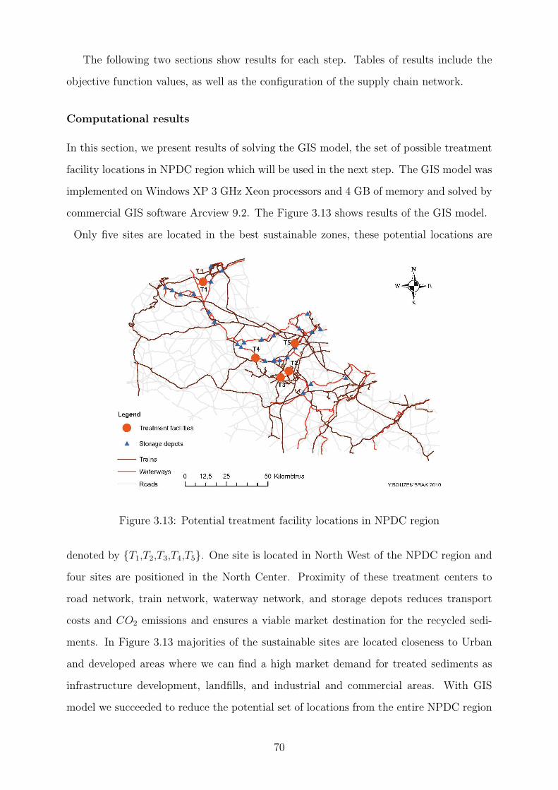
The following two sections show results for each step. Tables of results include the
objective function values, as well as the configuration of the supply chain network.
Computational results
In this section, we present results of solving the GIS model, the set of possible treatment
facility locations in NPDC region which will be used in the next step. The GIS model was
implemented on Windows XP 3 GHz Xeon processors and 4 GB of memory and solved by
commercial GIS software Arcview 9.2. The Figure 3.13 shows results of the GIS model.
Only five sites are located in the best sustainable zones, these potential locations are
Figure 3.13: Potential treatment facility locations in NPDC region
denoted by {T1,T2,T3,T4,T5}. One site is located in North West of the NPDC region and
four sites are positioned in the North Center. Proximity of these treatment centers to
road network, train network, waterway network, and storage depots reduces transport
costs and CO2 emissions and ensures a viable market destination for the recycled sedi-
ments. In Figure 3.13 majorities of the sustainable sites are located closeness to Urban
and developed areas where we can find a high market demand for treated sediments as
infrastructure development, landfills, and industrial and commercial areas. With GIS
model we succeeded to reduce the potential set of locations from the entire NPDC region
70

to five sustainable locations. This will speed up the process of finding the optimal supply
chain configuration in the next step.
3.5.2 STEP 2: Mathematical model solving supply chain net-
work design
Transportation costs
We start by determining distances between logistic actors in order to calculate the trans-
portation costs from suppliers to storage depots, from depots storage to treatment facilities
and from treatment facilities to customers. All these distances using railways, waterways
and roads as transportation mode are calculated using GIS Arcview.9.2 tools like Spa-
tial Analyst and Network Analyst (Figure 3.14). Transportation costs are calculated per
weight and distance. They depend on the distance, and the quantity to be transported.
The unit transportation cost for goods can be broken down to its main components: cap-
ital, fuel, lubricants, driver and maintenance costs. All expenses along the lifetime of a
vehicle are calculated.
Legend
Roads
Waterways
Trainways
.
0 20 40 60 8010Kilomètres BOUZEMBRAK.Y. 2010
Figure 3.14: Transportation modes in Nord Pas De Calais (NPDC) region
71

Opening, treatment and storage costs
- Opening costs: The facility opening cost implies establishing a treatment facility. There-
fore, it will change according to the place where it will be built. This cost variation is
due to the variation of ground and workforce costs; similarly production and storage costs
vary according to the location.
- Treatment costs: The treatment costs are composed of: equipment capital, energy con-
sumption, workforce, operational and maintenance costs. Only these costs have to be
taken into account. An average unit cost is assumed.
- Storage costs: The storage costs are composed of: storage equipment capital, energy
consumption, workforce, operational and maintenance costs.
CO2 Emissions
Air pollution generated by freight trains, barge and trucks affects negatively the envi-
ronment and the health of people. We estimate the external costs associated with two
general categories of emissions: air pollution and greenhouse gases. Assigning Euro values
to emissions generated per ton-km of freight transportation is inherently difficult.
Decision Makers choose the green technology of treatment facility. So, we assume that
only transportation means are sources of air pollution.
For CO2 emissions in France, we found in some ADEME (Agency of Environment and
Energy Management in France) reports, the CO2 emissions factors of three transportation
modes (Table 3.9).
Table 3.9: CO2 Emissions factors
Transportation Mode Roads Waterways Railways
CO2 Emissions (g/ton.km) 133.11 37.68 5.75
Computational results
In this section, we analyse the computational results obtained from the resolution of
the proposed mathematical model considering economic and environmental aspect. The
integration of CO2 emission taxes in the objective function represents the environmental
aspect in model (3.3)-(3.20). This model is applied to a real case of VNF company in
72

NPDC region. To illustrate the validity and the usefulness of the proposed model, several
numerical experiments are implemented and results are reported in this section. The
mathematical model was solved on a Windows Vista 2 GHz Core 2 Due PC with 3 Go of
memory by commercial software solver ILOG OPL 6.3/CPLEX 12.1.0.
- Environmental vs Economic supply chain:
In this section, we introduce the effect of varying ω1 and ω2 on the supply chain network
configuration. For this problem size, the computation time was negligible and the mixed
integer programming model contains 11 408 constraints and 4 876 decision variables.
Table 3.10 shows the impact of ω1 and ω2 on the supply chain network configuration
decisions and on the transportation mode used.
In Table 3.10, Weight represents values of the ω1 and ω2 used on the objective function.
Potential facilities column contains the set of the potential sites. % of transportation
mode column presents the mode of transport used en percentage. Finally the value of the
objective function expressed in (e).
Table 3.10: SCN Configuration varying ω1 and ω2
No Weight Potential facilities % of transportation
mode
Values(e)
ω1 ω2 T1 T2 T3 T4 T5 Roads Waters Rails Objective Value (e)
1 0 1 X X 3% 24% 73% 30 039 950
2 0.1 0.9 X X 3% 26% 71% 31 895 690
3 0.2 0.8 X X 1% 26% 73% 33 750 860
4 0.3 0.7 X X 1% 37% 63% 35 598 230
5 0.4 0.6 X X 1% 36% 63% 37 445 080
6 0.5 0.5 X X 0% 37% 63% 39 290 250
7 0.6 0.4 X X 0% 37% 63% 41 134 900
8 0.7 0.3 X X 0% 50% 50% 42 979 440
9 0.8 0.2 X X 0% 53% 47% 44 823 850
10 0.9 0.1 X X 0% 53% 47% 46 667 200
11 1 0 X X 13% 73% 14% 48 509 520
73
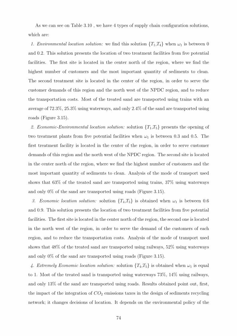
As we can see on Table 3.10 , we have 4 types of supply chain configuration solutions,
which are:
1. Environmental location solution: we find this solution {T1,T4} when ω1 is between 0
and 0.2. This solution presents the location of two treatment facilities from five potential
facilities. The first site is located in the center north of the region, where we find the
highest number of customers and the most important quantity of sediments to clean.
The second treatment site is located in the center of the region, in order to serve the
customer demands of this region and the north west of the NPDC region, and to reduce
the transportation costs. Most of the treated sand are transported using trains with an
average of 72.3%, 25.3% using waterways, and only 2.4% of the sand are transported using
roads (Figure 3.15).
2. Economic-Environmental location solution: solution {T1,T5} presents the opening of
two treatment plants from five potential facilities when ω1 is between 0.3 and 0.5. The
first treatment facility is located in the center of the region, in order to serve customer
demands of this region and the north west of the NPDC region. The second site is located
in the center north of the region, where we find the highest number of customers and the
most important quantity of sediments to clean. Analysis of the mode of transport used
shows that 63% of the treated sand are transported using trains, 37% using waterways
and only 0% of the sand are transported using roads (Figure 3.15).
3. Economic location solution: solution {T4,T5} is obtained when ω1 is between 0.6
and 0.9. This solution presents the location of two treatment facilities from five potential
facilities. The first site is located in the center north of the region, the second one is located
in the north west of the region, in order to serve the demand of the customers of each
region, and to reduce the transportation costs. Analysis of the mode of transport used
shows that 48% of the treated sand are transported using railways, 52% using waterways
and only 0% of the sand are transported using roads (Figure 3.15).
4. Extremely Economic location solution: solution {T4,T5} is obtained when ω1 is equal
to 1. Most of the treated sand is transported using waterways 73%, 14% using railways,
and only 13% of the sand are transported using roads. Results obtained point out, first,
the impact of the integration of CO2 emissions taxes in the design of sediments recycling
network; it changes decisions of location. It depends on the environmental policy of the
74

���
���
���
���
�
���
���
���� ������
���
�����������
��
��
���
��
��
� �� �� ��� ��� ��� ��� ��� ��� ��� � �� �� ��� ��� ��� ��� ��� ��� ���
��
����� ���� � �����
Figure 3.15: The transportation mode used varying ω1
company, if managers are environmental they will take the first solution, if they are looking
for the environmental and economic solution they should choose the second solution, and
if they want the economic scenario they should adopt the forth solution. This means that
using the model, supply chain managers are now able to see the impact of integration
of the CO2 taxes and multi-modality in the strategic decisions. That will help them to
decide the best strategic design of the supply chain.
CO2 taxes variation:
As in last subsection we varied ω1 and ω2 to see their effect on the SCN configuration. In
this paragraph, we extend the analysis to CO2 taxes γ. We fix the ωi (ω1 = 1 and ω2 =
1) and we increase the value of γ from 0 to 200 000 (e/ton).
The following Table 3.11 shows the impact of γ on the supply chain design decisions and
on the transportation mode used.
Supply chain configurations:
We present the optimal supply chain configurations obtained varying γ and a comparison
between values of objective function of two cases (γ=0) and (γ 6= 0).
For instance, in Table 3.11, for γ=0 the SC structure is { T4,T5 } and the objective function
75

Table 3.11: Supply chain configuration varying CO2 taxes
No γ (e/ton) Configuration Objective function(e) Difference (%)*
1 0 T4, T5 48 509 520 0.0%
2 10 T4, T5 48 509 822 0.0%
6 200 T4, T5 48 515 341 0.0%
7 300 T4, T5 48 518 166 0.0%
22 3000 T4, T5 48 583 363 0.2%
23 4000 T1, T5 48 606 223 0.2%
32 13000 T1, T5 48 792 915 0.6%
33 14000 T1, T4 48 809 384 0.6%
value is equal to 48 509 520. For γ=4000 the configuration is { T1,T5 } and the objective
value is 48 606 223. As we can see on the Table 3.11, we have 3 different solutions, { T4,T5
}, { T1,T5 } ,and { T1,T4 }. The first configuration is obtained when γ is between 0 and
3 000. The second network is obtained when γ is between 4 000 and 13 000. The last one
is fond when γ is higher than 14 000.
It can be observed, the optimal solution { T4,T5 } is approximately 0.2% cheaper than the
second configuration { T1,T5 } and approximately 0.6% cheaper than the third solution.
CO2 Emissions:
In this section, we present a comparison of CO2 emissions quantities obtained for (γ =
0) and (γ 6= 0). To get the quantity of CO2 emissions of the supply chain, we used the
equation (6.29). As we can observe on Table 3.12, the integration of environmental taxes
reduces the quantity of CO2 emissions to at least 70%. For γ = 10, the quantity of CO2
emission decreases to approximately 70% less than the case with γ = 0.
Analysis of Figure 3.16 shows that the most polluted configuration is the first one,
without carbon taxes, in this case the quantity of CO2 gazes is 980 (tons). This quantity
goes down to approximately 300 (tons) increasing γ to 10. As we can see also, we have
four levels of CO2 emissions: the fist level is obtained for γ between 10 and 600, the
average of CO2 emissions is equal to 285 (tons). The average of CO2 emissions drops to
an average of 238 (tons) in the second level when γ is between 600 and 4 000. In the third
76

Table 3.12: CO2 Emissions varying CO2 taxes γ
No γ (e/ton) CO2 Emissions (Tons) Difference (%)
1 0 980 0.0%
2 10 302 69.2%
6 200 286 70.8%
7 300 280 71.4%
22 3000 233 76.2%
23 4000 226 76.9%
32 13000 205 79.1%
33 14000 164 83.3%
level for γ between 4 000 and 13 000, the average of CO2 emissions is 205 (tons). Finally,
above 13 000, we obtained the fourth level where the average of CO2 is about 156 (tons).
Transportation Modes:
In this section, we show the effect of γ variation on the transportation modes used in
shipment of the sediment throughout the supply chain network.
As we can see on Table 3.13 , we have 5 types of supply chain configurations, which are:
Table 3.13: Transportation modes used varying CO2 taxes
Transportation Modes
No γ (e/ton) % Roads % Waters % Trains
1 0 9.3% 80.7% 10%
2 10 0.0% 78% 22%
6 200 0% 74.7% 25.3%
7 300 0% 54.7% 45.3%
22 3000 0% 52.0% 48.0%
23 4000 0% 36.7% 63.3%
32 13000 0.7% 36.7% 62.7%
33 14000 1.3% 25.3% 73.3%
1. Extremely Economic configuration: solution { T4,T5 } is obtained when γ is equal to
77
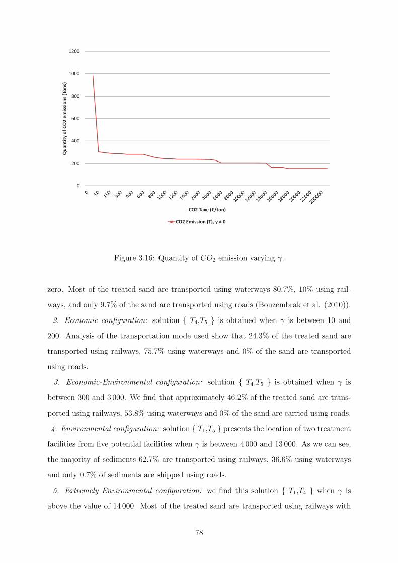
���
���
���
����
����
����������� ���������������
�
���
���
�� ������������
�� �������������������
Figure 3.16: Quantity of CO2 emission varying γ.
zero. Most of the treated sand are transported using waterways 80.7%, 10% using rail-
ways, and only 9.7% of the sand are transported using roads (Bouzembrak et al. (2010)).
2. Economic configuration: solution { T4,T5 } is obtained when γ is between 10 and
200. Analysis of the transportation mode used show that 24.3% of the treated sand are
transported using railways, 75.7% using waterways and 0% of the sand are transported
using roads.
3. Economic-Environmental configuration: solution { T4,T5 } is obtained when γ is
between 300 and 3 000. We find that approximately 46.2% of the treated sand are trans-
ported using railways, 53.8% using waterways and 0% of the sand are carried using roads.
4. Environmental configuration: solution { T1,T5 } presents the location of two treatment
facilities from five potential facilities when γ is between 4 000 and 13 000. As we can see,
the majority of sediments 62.7% are transported using railways, 36.6% using waterways
and only 0.7% of sediments are shipped using roads.
5. Extremely Environmental configuration: we find this solution { T1,T4 } when γ is
above the value of 14 000. Most of the treated sand are transported using railways with
78
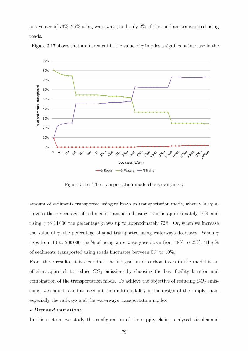
an average of 73%, 25% using waterways, and only 2% of the sand are transported using
roads.
Figure 3.17 shows that an increment in the value of γ implies a significant increase in the
���
���
���
���
���
���
��
��������
�������� �������
��
��
���
���
����� ����������
�� ���� �������� ��������
Figure 3.17: The transportation mode choose varying γ
amount of sediments transported using railways as transportation mode, when γ is equal
to zero the percentage of sediments transported using train is approximately 10% and
rising γ to 14 000 the percentage grows up to approximately 72%. Or, when we increase
the value of γ, the percentage of sand transported using waterways decreases. When γ
rises from 10 to 200 000 the % of using waterways goes down from 78% to 25%. The %
of sediments transported using roads fluctuates between 0% to 10%.
From these results, it is clear that the integration of carbon taxes in the model is an
efficient approach to reduce CO2 emissions by choosing the best facility location and
combination of the transportation mode. To achieve the objective of reducing CO2 emis-
sions, we should take into account the multi-modality in the design of the supply chain
especially the railways and the waterways transportation modes.
- Demand variation:
In this section, we study the configuration of the supply chain, analysed via demand
79

variation. Throughout, we will use the term Low demand case to denote demand cases
with 100 500 tons as annual customers average, the term Medium demand case to refer
to demand cases with annual customers average equal to 250 000 tons and the term High
demand case to mention to the increase in the annual costumers average to 402 000 tons.
- Low demand case
In this section, the average of annual customer demands is equal to 100 500 tons per year.
We generated 24 demand scenarios and the demand of each customer is assumed to be
fitted to normal distribution with 2 000 tons as the mean value and 40% of mean value
as the standard deviation. Clearly in this situation only one cleaning facility is necessary,
which has to work at full capacity. Table 3.14 presents only four scenarios from 24 ones
generated, for more detail see Table A.11. The optimal configurations of each demand
scenario are illustrated in Table 3.14.
In Table 3.14 optimal solution contains the objective function value of each experience,
Table 3.14: Low demand case
Treatment facility
Scenarios Objective function value (e) T1 T2 T3 T4 T5
S1 21 499 647 0 0 0 0 1
S6 22 557 098 1 0 0 0 0
S12 21 497 861 0 0 0 0 1
S20 22 511 297 0 0 0 0 1
expressed in Euro. Finally the treatment facility contains the set of location solution. For
instance, the deterministic design exhibits two different location solutions (T1) or (T5). It
is also interesting to point out that the configuration depends on demands scenario (Table
3.14).
- Medium demand case
For medium demand case, the demand rises to 250 000 tons per year. We generated 24
demand scenarios (Table A.12) and the demand of each customer is supposed to be fitted
to normal distribution with an average of 5 000 tons and a standard deviation equals to
2 000 tons. Given the treatment capacity of 150 000 tons per year, it turns that at least
two facilities have to be opened.
80
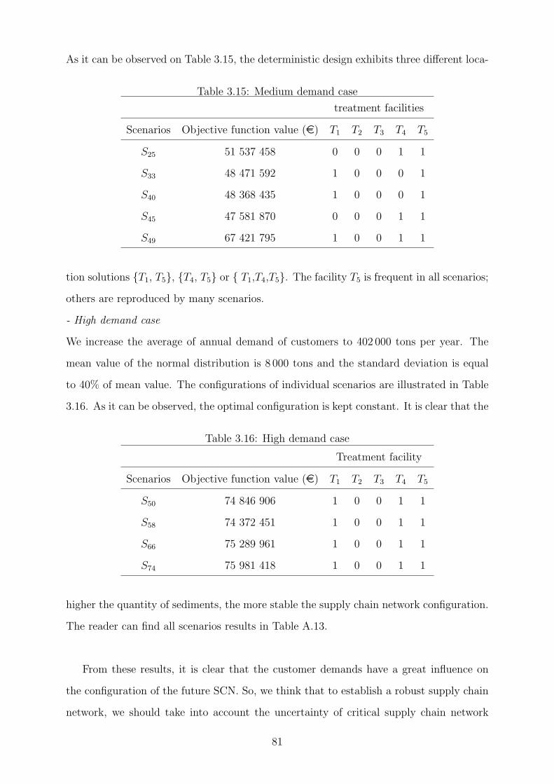
As it can be observed on Table 3.15, the deterministic design exhibits three different loca-
Table 3.15: Medium demand case
treatment facilities
Scenarios Objective function value (e) T1 T2 T3 T4 T5
S25 51 537 458 0 0 0 1 1
S33 48 471 592 1 0 0 0 1
S40 48 368 435 1 0 0 0 1
S45 47 581 870 0 0 0 1 1
S49 67 421 795 1 0 0 1 1
tion solutions {T1, T5}, {T4, T5} or { T1,T4,T5}. The facility T5 is frequent in all scenarios;
others are reproduced by many scenarios.
- High demand case
We increase the average of annual demand of customers to 402 000 tons per year. The
mean value of the normal distribution is 8 000 tons and the standard deviation is equal
to 40% of mean value. The configurations of individual scenarios are illustrated in Table
3.16. As it can be observed, the optimal configuration is kept constant. It is clear that the
Table 3.16: High demand case
Treatment facility
Scenarios Objective function value (e) T1 T2 T3 T4 T5
S50 74 846 906 1 0 0 1 1
S58 74 372 451 1 0 0 1 1
S66 75 289 961 1 0 0 1 1
S74 75 981 418 1 0 0 1 1
higher the quantity of sediments, the more stable the supply chain network configuration.
The reader can find all scenarios results in Table A.13.
From these results, it is clear that the customer demands have a great influence on
the configuration of the future SCN. So, we think that to establish a robust supply chain
network, we should take into account the uncertainty of critical supply chain network
81

parameters such as: demand and costs.
3.6 Concluding remarks
In this chapter, we have proposed a novel multi-criteria supply chain network design
methodology. Under economical, social, environmental and legislative aspects, we have
designed the optimal supply chain network.
Our methodology consists of two different steps. The first step looks for the best potential
facility locations to open in order to satisfy the different criteria using the GIS model and
the AHP method. The second step establishes the optimal supply chain design to achieve
customer demands and economic criteria using mixed integer programming model.
The results obtained point out, first, using GIS model to location potential facilities in the
design of sustainable supply chain network. In fact it provides a good way for integrating
many criteria and constraints such as: location sites far from the urban areas; sites should
be close to commercial zones, roads, railways and Landfills; plants should be far from nat-
ural area, airports and agriculture area, etc. With GIS model we succeeded to reduce the
potential set of locations from the entire NPDC region to only five sustainable locations.
This will speed up the process of finding the optimal supply chain configuration in the
next step.
Studying the impact of CO2 emissions in the SCND represents our second main contri-
bution in this chapter. Indeed, it changes the structure of the supply chain network. It
depends on the environmental policy of the company. This means that using the model,
supply chain managers could be able to see the impact of integration of the CO2 taxes
and multi-modality in the strategic decisions of supply chain design. That will help them
to select the best strategic supply chain network. From this chapter we have learned
that integration of environmental taxes in the model can be an efficient way to achieve
environmental goals, by choosing the best SCN and clean transportation modes. These
results have also confirmed that to reduce CO2 emissions, we should take into account
multi-modal network, in the design of the supply chain.
In the next chapter, we will extend the mathematical model of our methodology to a
multi-objective supply chain network model.
82

Chapter 4
Multi-objective Supply Chain
Network Design
This chapter continues and extends a line of work that we started in Chapter 3. We study
a supply chain network design problem with environmental concerns. We are interested in
the environmental investments decisions of the supply chain design phase and we propose
a multi-objective optimization model that captures a compromise between the total cost
and the environment influence. We use Goal Programming approach seeking to reach the
four goals placed by Decision Maker: (i) total costs goal, (ii) energy consumption costs
goal, (iii) waste treatment costs goal and (iv) CO2 emissions goal.
The strategic decisions considered in the model are treatment facilities location, building
technology selection and flow of material throughout the SC network.
We first discuss the integration of environmental aspects in Supply Chain Network Design
in Section 4.2. In Section 4.3, we present the Goal Programming (GP) method and the
techniques used to improve it. Section 4.4 proposes the definition of the problem and
the GP mathematical formulation. Section 4.5 presents numerical results illustrating and
comparing the performance of the GP model. In Section 4.6, we discuss conclusions from
our study and briefly summarize potential future research directions.
83

4.1 Introduction
Traditionally, the main objective of optimization models used in the design of supply chain
networks focused on the economic aspect (Goetschalcks and Fleischmann (2008)). How-
ever, as environment concerns grow, environmental aspects are also emerging at academic
and industry levels as decisive factors within the supply chain management context.
Nowadays, the investment towards logistics structures that considers both economic and
environmental performances is an important and current research topic.
This growing importance is driven mainly by the deterioration of the environment and the
new environmental regulations. However, companies must invest on the design and plan-
ning optimization of their logistic structures, while accounting for the trade-off between
profit and environment impact (Grossmann (2004), Barbosa-Povoa (2009), Srivastava
(2007), Guillen-Gosalbez and Grossmann (2009)).
Several authors have been working on the integration of CO2 emissions in supply chain
design. Recently Pan et al. (2009), showed that the logistical mutualisation is an effi-
cient approach to reducing CO2 emissions, at the same time they claimed that the rail
transport is an aspect that should be taken into account in order to achieve the objective
of reducing the CO2 emissions. The disadvantage of this model is that the economic
dimension is absent.
Paksoy et al. (2010), considered the green impact on a close-looped supply chain network
and tried to prevent more CO2 gas emissions and encourage the customers to use recy-
clable products via giving a small profit. They presented different transportation choices
between echelons according to CO2 emissions.
Wang et al. (2010) studied a supply chain network design problem with environmental
aspects. They interested in the environmental investments decisions in the design phase
and proposed a multi-objective optimization model that captures the trade-off between
the total cost and the environment influence. Authors considered two objective functions.
The first objective measures the sum of fixed set-up cost, environmental protection in-
vestment, total transportation cost and total handling cost. The second one measures the
total CO2 emission in all the supply chain. Wang et al showed that the model can be
applied as an effective tool in the strategic planning for green supply chain.
84
Guillen-Gosalbez and Grossmann (2009) also addressed the design and planning of sup-
ply chains formulating a bi-objective stochastic mixed-integer non linear program that
accounts simultaneously for the maximization of the net present value and the minimiza-
tion of the environmental impact for a given probability level.
Another related study is conducted by Hugo et al. (2005), who developed a multi-objective
optimisation approach for hydrogen SC networks, where they investigated trade-offs be-
tween investment and greenhouse gas emissions. Bojarski et al. (2009) addressed the
optimization of the design and planning of supply chains considering economic and envi-
ronmental issues.
The major drawbacks of these papers are the absence of incorporation of CO2 emissions
and multi-modality in supply chain network design. Also, only few studies have addressed
the impact of integrating environmental regulations, green house gases emissions, energy
consumption, green technology and carbon taxes Nagurney et al. (2006), emission trad-
ing (Stranlund (2007)) and carbon markets (Peace and Juliani, (2009)) on supply chain
network design.
In this context, this chapter deals with the design of a multi-objective supply chain net-
work in order to satisfy the customer demands and to respect the environmental require-
ments. We use Goal Programming approach seeking to reach the four goals placed by
Decision Maker: (i) total costs goal, (ii) energy consumption costs goal, (iii) waste treat-
ment costs goal and (iv) CO2 emissions goal.
The strategic decisions considered in the model are treatment facilities location, building
technology selection and flow of material quantities throughout the SC network. To solve
the model, we apply a Goal Programming approach, which is a single model and easy to
understand and to apply (Aouni and Kettani (2001)).
Finally, we conduct a comprehensive set of numerical studies and present the solutions
and their sensitivities to various parameters.
4.2 Goal Programming
A goal refers to criterion and a numerical level known as a target level, which the decision
maker desires to achieve on the criterion (Tamiz (2009)). There are three principal types
85

of goal that can occur in a goal programming model: achieve at most the target level,
achieve at least the target level and achieve the target level. A constraint is a restriction on
the decision variables that must be satisfied in order to implement the solution in practice
(Tamiz (2009)). This is different from the concept of a goal whose non-achievement does
no automatically make the solution non implementable.
The first Goal Programming (GP) formulation was proposed by Charnes et al. (1955).
At that period the term goal programming was not used as a model, but considered as an
adaptation of the linear programming. After six years the theory of the GP was defined by
Charnes and Cooper (1961), then by Ijiri (1965), Lee (1972) and Ignizio (1976), Romero
(1991), Jones et al. (1995) and Tamiz (2009).
According to Field (1973), the formulation of goal programming is characterised by one
or more goals which are directly incorporated in the objective function, through deviation
variables, that is, the objectives are written in the form of goals restrictions, where each
goal represents the value that intends to be reached. The goals can or not be reached
completely and, to allow this flexibility, deviation variables are used δ+ and δ−, indicating
how much the objective was surpassed or was lacked by that value respectively. Goal
programming searches a form of reaching the goals as closest as possible; the objective of
this technique is to minimize the sum of all the goal deviations.
There are several methods for specifying the corresponding weight values in GP, as detailed
by Ringuest (1992). Gass (1986) explained how a link can be established between the
Analytical Hierarchy Process (AHP) and GP. In fact, the weights derived from the pairwise
comparison of AHP can be incorporated directly into a GP model. Gass (1986) also
showed that in some cases the normalising weight is simply part of the whole weight that is
absorbed by the AHP weight determination. To model a multi-objective decision making
problem aiming at selecting the best warehouses, William (2007) combined the AHP and
goal programming. The AHP is used to give weights or priorities to the warehouses based
on two conflicting criteria; customer satisfaction level and operational cost. These weights
are incorporated in a GP model that considers system and goal constraints.
86

4.2.1 Normalisation Techniques
Incommensurable in a GP model, occurs when deviation variables measured in different
units are summed up directly. This simple summation will cause a deviation towards the
objectives with a larger magnitude. This deviation may lead to erroneous or misleading
results.
To overcome incommensurable in GP, researchers proposed the use of normalisation tech-
niques. One suggestion to overcome this difficulty, is to divide each objective through by
a normalising constant (i) pertaining to that objective, as shown in model (4.5). This
ensures that all objectives have roughly the same magnitude.
We are now able to show a simple achievement function of GP as follows:
Min
n∑
i=1
ωi(δ+i + δ−iki
) (4.1)
s.t fi(X) + δ−i − δ+i = gi i = 1, 2, ..., n. (4.2)
δ+i , δ−
i ≥ 0 i = 1, 2, ..., n. (4.3)
x ∈ F . (4.4)
(4.5)
where ωi is the weight of the i-th goal; fi(X) is the linear function of {xi, x2 , · · · , xn} for
the ith goal, gi is the aspiration level of the ith goal, δ+i and δ−i are positive and negative
deviations from the target value of the ith goal, respectively. i are normalising constants
of the i-th goal; F is a feasible set.
We will next discuss an application case to which this approach applies.
4.3 Problem Formulation
We start by introducing the SC problem that we have studied in Chapter 3, which is :
multi-level, multi-modal, multi-objective, single product and single period Supply Chain
Network (SCN). As before, The SCN contains four layers: suppliers, storage depots,
treatment facilities and customers. As illustrated in Figure 6.5, products are shipped
87
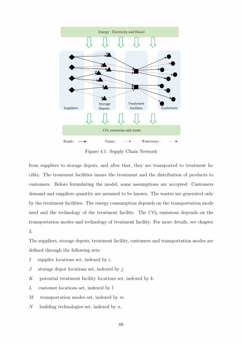
Roads : Trains : Waterways :
Energy : Electricity and Diesel
CO2 emissions and waste
����������
������� �
��������
����� ��������� �� ����� �
Figure 4.1: Supply Chain Network
from suppliers to storage depots, and after that, they are transported to treatment fa-
cility. The treatment facilities insure the treatment and the distribution of products to
customers. Before formulating the model, some assumptions are accepted: Customers
demand and suppliers quantity are assumed to be known. The wastes are generated only
by the treatment facilities. The energy consumption depends on the transportation mode
used and the technology of the treatment facility. The CO2 emissions depends on the
transportation modes and technology of treatment facility. For more details, see chapter
3.
The suppliers, storage depots, treatment facility, customers and transportation modes are
defined through the following sets:
I supplier locations set, indexed by i.
J storage depot locations set, indexed by j.
K potential treatment facility locations set, indexed by k.
L customer locations set, indexed by l.
M transportation modes set, indexed by m.
N building technologies set, indexed by n.
88

P goal level set, indexed by p.
Each goal should be assigned a weight γi to represent its importance and a goal value gi
that required to be achieved. The deviation variables of the goals are δ+i and δ+i . The unit
transportation costs of goods between supplier i and storage depot j using transporta-
tion mode m is µijm, the unit transportation costs of goods between storage depot j and
treatment facility k using transportation mode m is µjkm and µklm represents the unit
transportation costs of goods between treatment facility k and customer l using trans-
portation mode m.
ϑijm is the distance between supplier i and storage depot j using transportation mode m.
ϑjkm represents distance between storage depot j and treatment facility k using trans-
portation mode m. ϑklm represents distance between treatment facility k and customer l
using transportation mode m.
βm denotes the unit CO2 emission using transportation mode m. The unit CO2 emission
in treatment facility k with building technology n is βkn. Energy consumption parameters
are ρm and γkn. The first one represents the unit energy consumption costs using trans-
portation mode m and the second one denotes the unit energy consumption costs using
treatment facility k with building technology n. ηkn denotes the unit waste treatment
costs in treatment facility j with building technology n. γ is the environmental taxes. Dl
denotes the demand of the customer l.
In our problem, we consider two types of decision variables: treatment facility location
decisions will be taken based on the binary variables xkn that indicate whether treatment
facility k with building technology n is selected or not. Whereas, material flow related
decisions will be taken according to the value of the variables qijm which is the quantity
of products transported from node i to node j using transportation mode m.
4.3.1 Mathematical Model
In this section we will show the mathematical formulation of the inland waterways sedi-
ments treatment supply chain network.
We explicitly consider two objective functions: φ1 measures the total cost (4.6) and φ2
89

represents the total CO2 emission in all the supply chain network (4.7).
φ1 :Min OC + TC + LC + ECC +WTC (4.6)
φ2 :Min COE (4.7)
Where
- Opening Costs (denoted OC):
OC =∑
k∈K
∑
n∈N
(COkn · xkn) (4.8)
- Transportation Costs (denoted TC):
TC =
[
∑
i∈I
∑
j∈J
∑
m∈M
µijm · qijm +∑
j∈J
∑
k∈K
∑
m∈M
µjkm · qjkm +∑
k∈K
∑
l∈L
∑
m∈M
µklm · qklm
]
(4.9)
- Logistic Costs (denoted LC):
LC =∑
i∈I
∑
j∈J
∑
m∈M
CSj · qijm +∑
j∈J
∑
k∈K
∑
m∈M
CTk · qjkm (4.10)
- Energy Consumption Costs (denoted ECC):
ECC =∑
i∈I
∑
j∈J
∑
m∈M
ρm · ϑijm · qijm +∑
j∈J
∑
k∈K
∑
m∈M
ρm · ϑjkm · qjkm + (4.11)
∑
k∈K
∑
l∈L
∑
m∈M
ρm · ϑklm · qklm +∑
j∈J
∑
k∈K
∑
m∈M
∑
n∈N
γkn · qjkm
- Waste Treatment Costs (denoted WTC):
WTC =∑
j∈J
∑
k∈K
∑
m∈M
∑
n∈N
ηkn · qjkm (4.12)
- Total CO2 emissions (denoted COE):
COE =∑
i∈I
∑
j∈J
∑
m∈M
βm · ϑijm · qijm +∑
j∈J
∑
k∈K
∑
m∈M
βm · ϑjkm · qjkm + (4.13)
∑
k∈K
∑
l∈L
∑
m∈M
βm · ϑklm · qklm +∑
j∈J
∑
k∈K
∑
m∈M
∑
n∈N
βkn · qjkm
Subject to
Constraint (4.14) limits CO2 emissions quantities.
∑
i∈I
∑
j∈J
∑
m∈M
βm · ϑijm · qijm +∑
j∈J
∑
k∈K
∑
m∈M
βm · ϑjkm · qjkm + (4.14)
∑
k∈K
∑
l∈L
∑
m∈M
βm · ϑklm · qklm +∑
j∈J
∑
k∈K
∑
m∈M
∑
n∈N
βkn · qjkm ≤ COEmax
90

Constraint (4.15) limits the energy consumption.
∑
i∈I
∑
j∈J
∑
m∈M
ρm · ϑijm · qijm +∑
j∈J
∑
k∈K
∑
m∈M
ρm · ϑjkm · qjkm + (4.15)
∑
k∈K
∑
l∈L
∑
m∈M
ρm · ϑklm · qklm +∑
j∈J
∑
k∈K
∑
m∈M
∑
n∈N
γkn · qjkm ≤ ECCmax
Constraint (4.16) guarantees that the demand of the customers will be satisfied.
∑
k∈K
∑
m∈M
qklm = Dl ∀l ∈ C (4.16)
Constraint (4.17) imposes a capacity restriction for each storage depot.
∑
i∈I
∑
m∈M
qijm ≤ Qj ∀j ∈ J (4.17)
Constraint (4.18) limits the capacity of the treatment facilities.
∑
j∈J
∑
m∈M
qjkm ≤ Qk · xkn ∀k ∈ K, ∀n ∈ N (4.18)
Constraints (4.19), (4.20) enforce the flow conservation of the product.
∑
i∈I
∑
m∈M
qijm =∑
k∈K
∑
m∈M
qjkm ∀j ∈ J (4.19)
∑
j∈J
∑
m∈M
qjkm =∑
l∈L
∑
m∈M
qklm ∀k ∈ K (4.20)
Constraints (4.21), (4.22), (4.23) impose a capacity restriction of each mode of transport
throughout the network.
qijm ≤ Qijm ∀i ∈ I, ∀j ∈ J, ∀m ∈M (4.21)
qjkm ≤ Qjkm ∀j ∈ J, ∀k ∈ K, ∀m ∈M (4.22)
qklm ≤ Qklm ∀k ∈ K, ∀l ∈ L, ∀m ∈M (4.23)
Constraint (4.24) enforces the binary nature of the configuration decisions for the facilities.
xkn ∈ {0, 1} ∀k ∈ K, ∀n ∈ N (4.24)
Constraints (4.25), (4.26), (4.27) are standard integrality and non-negativity constraints.
qijm ≥ 0 ∀i ∈ I, ∀j ∈ J, ∀m ∈M (4.25)
qjkm ≥ 0 ∀j ∈ J, ∀k ∈ K, ∀m ∈M (4.26)
qklm ≥ 0 ∀k ∈ K, ∀l ∈ L, ∀m ∈M (4.27)
91

4.3.2 Goal Programming Model
Among the different approaches available to solve the multi-objective supply chain net-
work design, the GP method seems to be the most promising.
Goal Programming approach were used seeking to reach the following goals: g1, g2, g3
and g4 placed by the Decision Maker.
The first goal (4.30) seeks assigning as at most total costs target level g1 (e). The second
goal (4.31) aims to achieve at most the energy consumption target level g2 (e). The third
goal (4.31) aims to achieve at most the waste treatment cost target level g3 (e). The
fourth goal (4.32) seeks achieve at most the CO2 emissions target level g4 (T).
Objective function (4.28) aims at minimizing the deviations from the goals g1, g2, g3 and
g4.
Min∑
p∈P
ωp(δ+p + δ−pkp
) (4.28)
where ωp is the weight of the p-th goal and kp is a constant ensures that all objectives
have roughly the same magnitude.
Subject to
Total cost goal level (denoted by g1).
∑
k∈K
∑
n∈N
(COkn · xkn) +∑
i∈I
∑
j∈J
∑
m∈M
µijm · qijm +∑
j∈J
∑
k∈K
∑
m∈M
µjkm · qjkm + (4.29)
∑
k∈K
∑
l∈L
∑
m∈M
µklm · qklm +∑
i∈I
∑
j∈J
∑
m∈M
CSj · qijm +∑
j∈J
∑
k∈K
∑
m∈M
CTk · qjkm +
∑
i∈I
∑
j∈J
∑
m∈M
ρm · ϑijm · qijm +∑
j∈J
∑
k∈K
∑
m∈M
ρm · ϑjkm · qjkm +
∑
k∈K
∑
l∈L
∑
m∈M
ρm · ϑklm · qklm +∑
j∈J
∑
k∈K
∑
m∈M
∑
n∈N
γkn · qjkm +
∑
j∈J
∑
k∈K
∑
m∈M
∑
n∈N
ηkn · qjkm + δ−1 − δ+1 = g1
Energy Consumption Costs goal (denoted by g2).
∑
i∈I
∑
j∈J
∑
m∈M
ρm · ϑijm · qijm +∑
j∈J
∑
k∈K
∑
m∈M
ρm · ϑjkm · qjkm + (4.30)
∑
k∈K
∑
l∈L
∑
m∈M
ρm · ϑklm · qklm +∑
j∈J
∑
k∈K
∑
m∈M
∑
n∈N
γkn · qjkm + δ−2 − δ+2 = g2
Waste treatment Costs goal (denoted by g3).
∑
j∈J
∑
k∈K
∑
m∈M
∑
n∈N
ηkn · qjkm + δ−3 − δ+3 = g3 (4.31)
92

Total CO2 emissions goal (denoted by g4).
∑
i∈I
∑
j∈J
∑
m∈M
βm · ϑijm · qijm +∑
j∈J
∑
k∈K
∑
m∈M
βm · ϑjkm · qjkm + (4.32)
∑
k∈K
∑
l∈L
∑
m∈M
βm · ϑklm · qklm +∑
j∈J
∑
k∈K
∑
m∈M
∑
n∈N
βkn · qjkm + δ−4 − δ+4 = g4
Constraint (4.33) limits CO2 emissions.
∑
i∈I
∑
j∈J
∑
m∈M
βm · ϑijm · qijm +∑
j∈J
∑
k∈K
∑
m∈M
βm · ϑjkm · qjkm + (4.33)
∑
k∈K
∑
l∈L
∑
m∈M
βm · ϑklm · qklm +∑
j∈J
∑
k∈K
∑
m∈M
∑
n∈N
βkn · qjkm ≤ COEmax
Constraint (4.35) limits Energy consumption.
∑
i∈I
∑
j∈J
∑
m∈M
ρm · ϑijm · qijm +∑
j∈J
∑
k∈K
∑
m∈M
ρm · ϑjkm · qjkm + (4.34)
∑
k∈K
∑
l∈L
∑
m∈M
ρm · ϑklm · qklm +∑
j∈J
∑
k∈K
∑
m∈M
∑
n∈N
γkn · qjkm ≤ ECCmax
Constraint (4.35) guarantees that the demand of the customers will be satisfied.
∑
k∈K
∑
m∈M
qklm = Dl ∀l ∈ C (4.35)
Constraint (4.36) imposes a capacity restriction for each storage depot.
∑
i∈I
∑
m∈M
qijm ≤ Qj ∀j ∈ J (4.36)
Constraint (4.37) limits the capacity of the treatment facilities.
∑
j∈J
∑
m∈M
qjkm ≤ Qk · xkn ∀k ∈ K, ∀n ∈ N (4.37)
Constraints (4.38), (4.39) enforce the flow conservation of the product.
∑
i∈I
∑
m∈M
qijm =∑
k∈K
∑
m∈M
qjkm ∀j ∈ J (4.38)
∑
j∈J
∑
m∈M
qjkm =∑
l∈L
∑
m∈M
qklm ∀k ∈ K (4.39)
93

Constraints (4.40), (4.41), (4.42) impose a capacity restriction of each mode of transport
throughout the network.
qijm ≤ Qijm ∀i ∈ I, ∀j ∈ J, ∀m ∈M (4.40)
qjkm ≤ Qjkm ∀j ∈ J, ∀k ∈ K, ∀m ∈M (4.41)
qklm ≤ Qklm ∀k ∈ K, ∀l ∈ L, ∀m ∈M (4.42)
Constraint (4.43) enforces the binary nature of the configuration decisions for the facilities.
xkn ∈ {0, 1} ∀k ∈ K, ∀n ∈ N (4.43)
Constraints (4.44), (4.45), (4.46) are standard integrality and non-negativity constraints.
qijm ≥ 0 ∀i ∈ I, ∀j ∈ J, ∀m ∈M (4.44)
qjkm ≥ 0 ∀j ∈ J, ∀k ∈ K, ∀m ∈M (4.45)
qklm ≥ 0 ∀k ∈ K, ∀l ∈ L, ∀m ∈M (4.46)
Constraint (4.47)Positive and negative deviational variable for i-th goal.
δ+p , δ−
p ≥ 0 ∀p ∈ P (4.47)
In the next section, we will give computational results of this model, as well as the
interpretation and analyse of the results.
4.4 Computational Results
In order to be able to analyse the behaviour of the optimal SC configuration, we will first
derive a general multi-objective results.
Experiments were performed using a computer with 2 GHz Windows Vista 2 GHz Core
2 Due PC and 3 GB RAM. Both models are coded using ILOG OPL 6.3 and solved
using CPLEX 12.1. The solver is set to solve integer problems using branch-and-bound
algorithm .
Before we describe our results, we first briefly discuss how we determine the Goal Pro-
gramming weights.
94

4.4.1 Goal Programming weights
To determine the corresponding weight values in GP, we used AHP method (see, section
3.3.1). The weights of each goal can be observed in Table 4.1. These values are fixed by
the Decision Maker (DM).
As shown in Table 4.1, the number 1 indicates the equal importance of the goals. The
Table 4.1: The Goal Programming weights
g1 g2 g3 g4 Weights
g1 1 0.33 0.25 4 0.16
g2 3 1 1 6 0.39
g3 4 1 1 3 0.37
g4 0.25 0.17 0.33 1 0.08
Total 8.25 2.50 2.58 14 1
number 3, indicates that g2 is moderately important than g1. The scale 4, indicates that
g3 is considerably more important than g1. Finally, 6 indicates that g2 is strongly more
important than g4. The weight of total cost criterion g1 is equal to 0.16 and the weight
of CO2 emission g3 is equal to 0.37. This means, ω1 = 0.16, ω2 = 0.39, ω3 = 0.37 and ω4
= 0.08.
We are now ready to start the resolution of our model.
4.4.2 Solutions
In this section, we will employ the classical approach to determine the optimal structure
of the problem and to have an idea about the different goal level. It is well-known that
there exist multiple non-dominated solutions for a multi-objective optimization problem.
Those solutions are called Pareto optimal solutions.
First of all, the bi-objective model (4.6)-(4.27) has two objective functions, the objective
value of these two functions are represented by φ1 and φ2, respectively. Then, we solve
the Model (4.6)-(4.27) with each objective function separately and get the objective value
φ∗
1 and φ∗
2 corresponding to objective one and two, respectively. Finally, we generate the
corresponding Pareto point set.
95
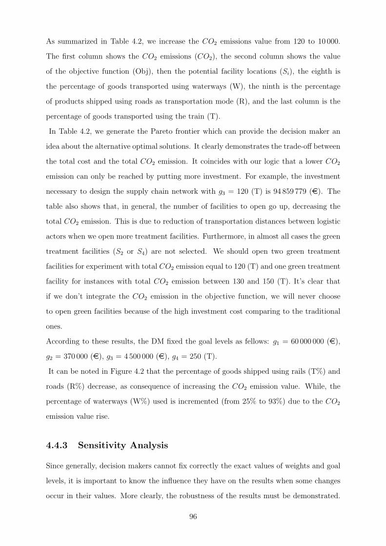
As summarized in Table 4.2, we increase the CO2 emissions value from 120 to 10 000.
The first column shows the CO2 emissions (CO2), the second column shows the value
of the objective function (Obj), then the potential facility locations (Si), the eighth is
the percentage of goods transported using waterways (W), the ninth is the percentage
of products shipped using roads as transportation mode (R), and the last column is the
percentage of goods transported using the train (T).
In Table 4.2, we generate the Pareto frontier which can provide the decision maker an
idea about the alternative optimal solutions. It clearly demonstrates the trade-off between
the total cost and the total CO2 emission. It coincides with our logic that a lower CO2
emission can only be reached by putting more investment. For example, the investment
necessary to design the supply chain network with g3 = 120 (T) is 94 859 779 (e). The
table also shows that, in general, the number of facilities to open go up, decreasing the
total CO2 emission. This is due to reduction of transportation distances between logistic
actors when we open more treatment facilities. Furthermore, in almost all cases the green
treatment facilities (S2 or S4) are not selected. We should open two green treatment
facilities for experiment with total CO2 emission equal to 120 (T) and one green treatment
facility for instances with total CO2 emission between 130 and 150 (T). It’s clear that
if we don’t integrate the CO2 emission in the objective function, we will never choose
to open green facilities because of the high investment cost comparing to the traditional
ones.
According to these results, the DM fixed the goal levels as fellows: g1 = 60 000 000 (e),
g2 = 370 000 (e), g3 = 4500 000 (e), g4 = 250 (T).
It can be noted in Figure 4.2 that the percentage of goods shipped using rails (T%) and
roads (R%) decrease, as consequence of increasing the CO2 emission value. While, the
percentage of waterways (W%) used is incremented (from 25% to 93%) due to the CO2
emission value rise.
4.4.3 Sensitivity Analysis
Since generally, decision makers cannot fix correctly the exact values of weights and goal
levels, it is important to know the influence they have on the results when some changes
occur in their values. More clearly, the robustness of the results must be demonstrated.
96

Table 4.2: Solutions
Potential facilities Transportation mode
CO2 (T) Obj(e) S1 S2 S3 S4 S5 W (%) R (%) T (%)
120 94 859 779 1 1 1 1 0 25% 17% 58%
130 74 122 738 1 0 1 1 0 29% 17% 54%
140 59 143 025 1 1 0 0 0 37% 9% 55%
150 59 128 842 1 0 0 1 0 24% 13% 63%
160 56 132 771 1 0 1 0 0 21% 10% 69%
170 56 128 527 1 0 1 0 0 24% 6% 70%
180 56 127 934 1 0 1 0 0 25% 6% 69%
190 56 103 496 1 0 0 0 1 33% 12% 55%
200 56 083 323 1 0 0 0 1 33% 12% 55%
300 56 073 586 1 0 0 0 1 37% 17% 46%
400 56 083 612 1 0 0 0 1 44% 17% 39%
500 56 096 567 1 0 0 0 1 41% 25% 34%
600 56 110 390 1 0 0 0 1 39% 31% 30%
700 56 124 249 1 0 0 0 1 55% 6% 39%
800 56 138 139 1 0 0 0 1 55% 8% 38%
900 56 152 182 1 0 0 0 1 55% 9% 35%
1 000 56 166 444 1 0 0 0 1 58% 10% 32%
1 500 56 244 119 1 0 0 0 1 53% 19% 28%
2 000 56 323 797 1 0 0 0 1 55% 17% 28%
3 000 56 483 513 1 0 0 0 1 59% 13% 28%
4 000 56 643 206 1 0 0 0 1 64% 8% 28%
5 000 56 837 725 0 0 1 0 1 93% 7% 0%
6 000 57 070 118 1 0 0 0 1 93% 7% 0%
8 000 57 527 431 1 0 0 0 1 93% 7% 0%
9 000 57 757 436 0 0 1 0 1 93% 7% 0%
10 000 57 987 278 1 0 0 0 1 93% 7% 0%
97

���
���
���
���
���
����
��� �� ����
��
���
���
���
��
���
���
� �
���
���
���
���
���
���
���
��
���
���
���
���
���
����
����
����
����
���
����
����
����
����
�����
������������
��� ���������
�
��
��
Figure 4.2: Transportation mode used (%)
Therefore, an important step in many applications of multi-objective decision making is
to perform a sensitivity analysis on these parameters. Let’s start with ωi weights variation
ωi variation
In order to show the sensitivity of the numerical solution with respect to the values of
ωi, we conduct experiments with ωi variation. Table 4.3 focuses only on the results of
10 generated instances, where ωi values are not far from the ones fixed previously by the
Decision Maker (see Table 4.1). According to the obtained values of ωi using AHP, ω1 is
varied from 0.1 to 0.5, ω2 is varied from 0.1 to 0.7, ω3 is increased from 0.1 to 0.6 and ω4
is varied from 0.1 to 0.2. When ωi are varied manually the others parameters are fixed :
g1 = 60 000 000 (e), g2 = 370 000 (e), g3 = 4500 000 (e), g4 = 250 (T).
In all cases, we obtained the same supply chain structure composed of two treatment
facilities {S1, S4} a traditional treatment facility S1 and a green facility S4 (see, Table
4.3). In instance 4, we have the same SC configuration and a small variation in the
percentages of the transportation modes used. The waterways use decrease from 55% to
98
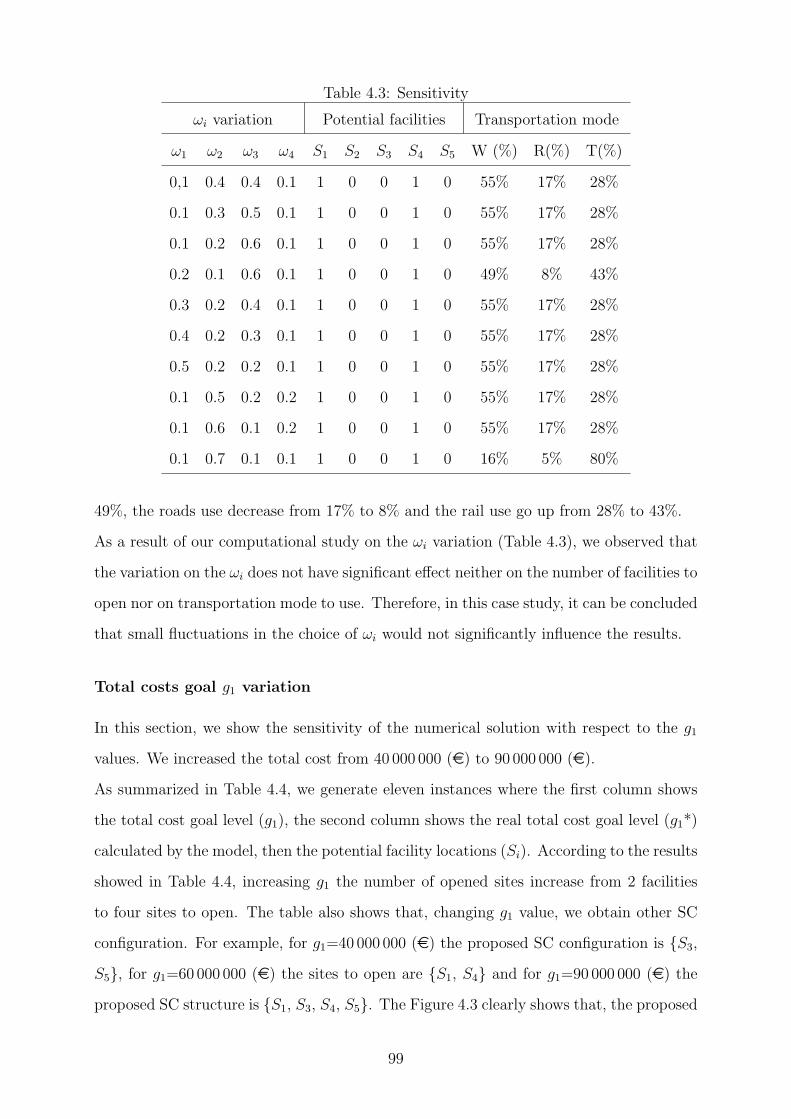
Table 4.3: Sensitivity
ωi variation Potential facilities Transportation mode
ω1 ω2 ω3 ω4 S1 S2 S3 S4 S5 W (%) R(%) T(%)
0,1 0.4 0.4 0.1 1 0 0 1 0 55% 17% 28%
0.1 0.3 0.5 0.1 1 0 0 1 0 55% 17% 28%
0.1 0.2 0.6 0.1 1 0 0 1 0 55% 17% 28%
0.2 0.1 0.6 0.1 1 0 0 1 0 49% 8% 43%
0.3 0.2 0.4 0.1 1 0 0 1 0 55% 17% 28%
0.4 0.2 0.3 0.1 1 0 0 1 0 55% 17% 28%
0.5 0.2 0.2 0.1 1 0 0 1 0 55% 17% 28%
0.1 0.5 0.2 0.2 1 0 0 1 0 55% 17% 28%
0.1 0.6 0.1 0.2 1 0 0 1 0 55% 17% 28%
0.1 0.7 0.1 0.1 1 0 0 1 0 16% 5% 80%
49%, the roads use decrease from 17% to 8% and the rail use go up from 28% to 43%.
As a result of our computational study on the ωi variation (Table 4.3), we observed that
the variation on the ωi does not have significant effect neither on the number of facilities to
open nor on transportation mode to use. Therefore, in this case study, it can be concluded
that small fluctuations in the choice of ωi would not significantly influence the results.
Total costs goal g1 variation
In this section, we show the sensitivity of the numerical solution with respect to the g1
values. We increased the total cost from 40 000 000 (e) to 90 000 000 (e).
As summarized in Table 4.4, we generate eleven instances where the first column shows
the total cost goal level (g1), the second column shows the real total cost goal level (g1*)
calculated by the model, then the potential facility locations (Si). According to the results
showed in Table 4.4, increasing g1 the number of opened sites increase from 2 facilities
to four sites to open. The table also shows that, changing g1 value, we obtain other SC
configuration. For example, for g1=40 000 000 (e) the proposed SC configuration is {S3,
S5}, for g1=60 000 000 (e) the sites to open are {S1, S4} and for g1=90 000 000 (e) the
proposed SC structure is {S1, S3, S4, S5}. The Figure 4.3 clearly shows that, the proposed
99

Table 4.4: Total costs goal g1 variation
g1 variation Potential facilities Transportation mode
g1 g1* S1 S2 S3 S4 S5 W(%) R(%) T(%)
40 000 000 59 150 000 0 0 1 1 0 82% 2% 16%
45 000 000 59 150 000 0 0 1 1 0 82% 2% 16%
50 000 000 59 150 000 0 0 1 1 0 81% 2% 17%
55 000 000 59 150 000 0 0 1 1 0 82% 2% 16%
60 000 000 60 000 000 1 0 0 1 0 55% 17% 28%
70 000 000 74 096 000 1 0 0 1 1 71% 2% 26%
80 000 000 80 014 000 0 1 0 1 1 69% 2% 29%
90 000 000 90 000 000 1 0 1 1 1 64% 12% 24%
�
�
�� ��������
�
�
�
�� �� �� �� �� �� �� �� � � �
����������
��������������
�� �� ��
�����
Figure 4.3: Number of opened facilities
100

���
���
���
���
���
���
���������
�� �� ����
��
���
� ��
��
���
���
���
�� �� �� �� �� �� �� ��
�������
��������������
� ��
Figure 4.4: Total costs goal g1 variation
SC configuration of all instances contain at least one green treatment facility. It seems
that, the presence of a green treatment facility in all solutions, is due to the CO2 emission
goal value fixed to 250 (T), the energy consumption goal and the waste treatment goal.
Figure 4.4 shows that increasing the total cost value g1, the percentage of goods shipped
using rails (T%) and roads (R%) goes up.
Energy consumption goal g2 variation
We now consider how the supply chain configuration and the transportation modes used
behave as the g2 level varies, which can be seen in Table 4.5. In this case g2 varied from
3 500 000 (e) to 6 500 000 (e).
The optimal SC structure of each instance are illustrated in Table 4.5. It is found that 2
facilities are built up. They are {S1, S4} or {S2, S5}, and in each solution we found a green
site to build (S2 or S4). According to the results presented in Table 4.5, increasing the
goal level g2, the percentage of goods transported using waterways transportation mode
decreases from 55% to 15%, the percentage of products shipped using roads transportation
mode goes down from 17% to 0% and the use of rail to transport the goods rises from
28% to 85% (see, Figure 4.5).
101

Table 4.5: Energy consumption goal g2 variation
g2 variation Potential facilities Transportation mode
g2 g2* S1 S2 S3 S4 S5 W(%) R(%) T(%)
3 500 000 4 552 000 1 0 0 1 0 55% 17% 28%
4 000 000 4 552 000 1 0 0 1 0 55% 17% 28%
4 500 000 4 550 000 1 0 0 1 0 55% 17% 28%
5 000 000 5 000 000 1 0 0 1 0 61% 20% 18%
5 500 000 5 500 000 0 1 0 0 1 15% 1% 84%
6 000 000 5 610 800 0 1 0 0 1 15% 0% 85%
6 500 000 5 610 800 0 1 0 0 1 15% 0% 85%
CO2 emissions goal g4 variation
The final aspect studied is CO2 emissions variation impact on the supply chain structure.
In this case, the carbon goal will increase (Figure 4.6) and all other parameters are fixed.
As summarized in Table 4.6, we increase g4 value from 100 to 15 000. The first column
shows the CO2 emission goal level (g4), the second the real CO2 emission goal level (g4*)
considered by the model and the rest of the columns have the same signification as in
Tables presented before.
Regarding the computational results, it is important to note the following. As shown in
Table 4.6 the number of facilities opened, is always equal to 2 sites and for each instance
the solution contains at least a green building (S2 or S4), due to the impact of g2 and
g4 goals, fixed by DM which forces the supply chain to use the green technology. Also,
increasing the g4 the use of waterways to transport goods increase from 39% to 100%,
the percentage of goods transported using roads fluctuate between 0% and 58%, and the
percentage of products shipped using train go down from 46% to 0%. Based on these
results, we can conclude that g4 value has influence in the SC configuration and the
transportation mode to use.
Figure 4.6 confirms that the g4 value variation has influence on the transportation
mode selected.
102

���
���
���
���
���
��
�� �� ����
���
��
��
���
���
���
��� � ��� � ��� � ���
��������������
�� ����������������������
���
���
����
Figure 4.5: Energy Consumption Costs
Table 4.6: CO2 emissions goal g4 variation
g4 variation Potential facilities Transportation mode
g4 g4* S1 S2 S3 S4 S5 W (%) R (%) T(%)
100 140.75 1 0 0 1 0 39% 15% 46%
150 150 1 0 0 1 0 37% 15% 48%
200 200 1 0 0 1 0 50% 15% 35%
250 250 1 0 0 1 0 55% 17% 28%
300 300 0 1 1 0 0 57% 12% 32%
400 400 0 0 1 1 0 78% 12% 10%
500 500 0 0 1 1 0 80% 13% 7%
1 000 1 000 0 0 0 1 1 42% 58% 0%
1 500 1 500 0 1 0 0 1 38% 48% 13%
2 000 2 000 0 0 0 1 1 80% 20% 0%
3 000 3 000 0 0 0 1 1 48% 52% 0%
4 000 4 000 0 0 0 1 1 51% 49% 0%
5 000 5 000 0 0 0 1 1 91% 9% 0%
10 000 10 000 0 1 0 1 0 41% 0% 59%
15 000 15 000 0 1 0 1 0 100% 0% 0%
103

���
���
����
����
��� �� ����
���
��
���
���
���
��� � � ��� � � ��� ��� �� ���� � �� ���� ���� ���� ��� ����� � ���
�������������
��� ��������
���
����
�����
Figure 4.6: CO2 emissions
4.5 Conclusions
In this Chapter, a multi-objective supply chain network design problem is addressed. The
problem is formulated as a goal programming model which aims at achieving four objec-
tives. The model represents a real case of supply chain network of an inland waterways
company in France. In this work, an approach for designing environmental SC has been
presented. The model consisted of a multi-objective optimization of economics and en-
vironmental goals. The model considered the long-term strategic decisions: treatment
facility location, transportation modes and material flux.
Sensitivity analysis for the case study is conducted and we check that, improving the
building technology and increasing the facility number in the supply chain can decrease
CO2 emission of the whole network. Regarding to the influence of some parameters on
the SC configuration and transportation mode used, we find that small variability of goals
weight ωi does not affect the solution of our case study.
Finally, in next chapter, we will present a heuristic to solve large scale SCND problems.
104

Chapter 5
Heuristic Approach to large scale
Supply Chain Network Design
Problem
The Supply Chain Network (SCN) should be designed in the way that could meet the cus-
tomer needs with an efficient cost. Nowadays, the structure of the supply chain network
is complex and has a considerable size. However, Supply Chain Network Design (SCND)
problems are hard to solve. Such network design problems belong to the class of NP-
hard problems, as several other well-known NP-hard facility location problems(Bloemhof-
Ruwaard et al. (1994), Cornuejols et al. (1991)).
In this chapter, a novel heuristic solution method is developed based on a decomposi-
tion technique, to solve large scale supply chain network design problems. This solution
method, specifically, designed for real size SCN problems that exact methods failed to
solve. The heuristic method is tested on real case instances, and it is compared to an
exact method in solving small instances. Results show that our heuristic outperforms the
exact method in terms of computational time and the size of problems solved.
5.1 Introduction
As we said in chapter 2, for small size supply chain network design problems, exact meth-
ods, such as Branch-and-Bound can be used to solve these problems. For large scale ones,
105
exact methods fail because the size of the solution space increases exponentially with the
number of constraints and variables in the network. In these cases heuristics methods
based on Lagrangian relaxation (Pirkul and Jayaraman (1997), Fisher (1985)), Bender
decomposition (Geoffrion and Graves (1974), Benders (1962)), Decomposition techniques
(Sahina and Saral (2007), Jang et al. (2002)) and many others techniques were proposed
to solve the SCND problems in a reasonable computation time.
To cope with this complexity, many researches divided the supply chain network into
several stages, such as: Ereng et al. (1999), Pontrandolfo and Okogbaa (1999) and Vidal
and Goetschalcks (1997).
To solve the supply chain network design problem, Jang et al. (2002) decomposed the
entire supply chain network into three sub-networks: the inbound network, distribution
network and outbound network. The first sub-problem consists of all suppliers to the
manufacturing plants, the second one includes facilities where the final products are man-
ufactured and the distribution facilities, the final sub-network consists of customers and
distributors close to customers. Authors proposed solution methodologies based on the
Lagrangian relaxation for each sub-network. They solved instances that have from 5 to
15 plants, from 10 to 20 warehouses, 10 customers and 10 products.
Lee and Dong (2008) explored the logistic network design for end-of-lease computer prod-
ucts recovery. Due to the problem complexity and the large number of variables and
constraints, they developed a two-stage heuristic approach to decompose the integrated
design of the multi-echelon forward and reverse logistics distribution networks into a
location-allocation problem and a revised network flow problem. Authors generated com-
putational results from a set of twenty-five test problems and the largest instance is
composed of 30 potential treatment facilities, 40 potential hybrid facilities and 100 cus-
tomers. Results suggested that the heuristic solution algorithm performs well in terms
of solution quality and computational time. The average gap between the final solution
obtained by the proposed heuristic approach and the lower bound obtained by CPLEX
ranges from 4% to 12%.
Cheng and Wang (2009) presented a decomposition procedure to solve distribution prob-
lems. They proposed a heuristic approach in which they decomposed a complex global
distribution problem into a combination of sub-problems with basic structures as inde-
106

pendent as possible to each other. The idea of their heuristic decomposition procedure
is to divide the large-scale global distribution into some identified sub-problems such as:
facility location problem, location-allocation problem, hub location problem, transporta-
tion problem, travelling salesman problem, vehicle routing problem, etc. Then, each
sub-problem is solved and the global solution is the sum of all these solutions.
Arntzen et al. (1995) presented a multi-period, multi-commodity mixed integer model
to optimize a global supply chain. The objective function includes variable production,
inventory, and shipping costs; fixed production costs, and savings from credit earned for
re-exporting products. They claimed that they solved models that had from 2000 to 6000
constraints and from 5000 to 20000 variables. It is not clear from the article the exact
method of solution applied, but they claimed that using non traditional methods, such as
row factorization and cascaded problem solution, allowed them to get impressive results
and always optimal solutions.
Cole (1995) presented a capacitate fixed-charge multi-commodity network flow model with
side constraints. The side constraints are the non-linear inventory service level constraints
resulting from the assumption of normally distributed demands. He suggested two solu-
tion procedures, and tested three example problems. The largest instance had 4 products,
9 customers, 3 potential plant locations, and 6 potential warehouse locations.
Goetschalckx et al. (1994) presented a generic model for the strategic design of production-
distribution systems. To solve the generic model, they introduced heuristic method that
significantly reduced the solution times compared to standard MIP solutions by a com-
mercial solver. Other heuristic algorithms are presented by Fleischmann et al. (2001) and
Geoffrion et al. (1978).
As evident from the above discussion, first, the decomposition resolution approach is less
used in SCND problems. The lack of these decomposition schemes may be explained by
the fact that due to the multi-level structure of a supply chain network and the interac-
tion of strategic decisions across several levels, it becomes more difficult to decompose the
problem into easier sub-problems. Second, the existing resolution approaches for supply
chain design problems are suited for very small size problems.
How can we get a solution of large scale SCND problem in a reasonable time?
To answer this question, we propose a heuristic algorithm based on decomposition tech-
107

nique. Our current study represents a significant improvement over past research by pre-
senting a unified model of the problem that includes numbers, locations and capacities of
warehouses and distribution centers to open and goods quantities to transport throughout
the supply chain network. Also, an efficient heuristic solution procedure based on decom-
position approach is developed in order to get good solution in an acceptable CPU time.
Computational tests with up to 1500 customers, 220 potential warehouses, 220 potential
distribution centers and 220 suppliers are reported.
The rest of the chapter is organized as follows. In section 5.2, the mathematical model
of the SCND problem is introduced. In section 5.3 the three-phase heuristic algorithm
based on decomposition is explained in detail. Then the heuristic phases are discussed and
applied to an application case in section 5.4. In section 5.5, some computational results
about the performance of heuristic are presented. Finally, some concluding remarks are
summarised in section 5.6.
5.2 Mathematical Model
In this section, we present the SCN problem and his mathematical formulation , then we
show the first computational results of the model solved using a commercial solver like
Cplex.
The potential design of a supply chain being considered (see Figure 5.1), is composed of
suppliers, warehouses, distribution centres, and sellers. As depicted in Figure 5.1, prod-
ucts are shipped from suppliers to warehouses, where goods are prepared to be sent to the
next level. Then, they are transported to distribution centers. The distribution centers
insure the storage and the distribution of products to sellers. Warehouses are defined as
the facility where products are received and married with goods going to the same des-
tination, then shipped at the earliest opportunity, without going into long-term storage.
They are located near suppliers and distribution centers. Distribution centers are ones
located near customers and handled most products in four cycles (receive, store, pick, and
ship).
The main assumptions used in the problem formulation are as follow:
–All demands of customers must be satisfied and no returned products from customers
108
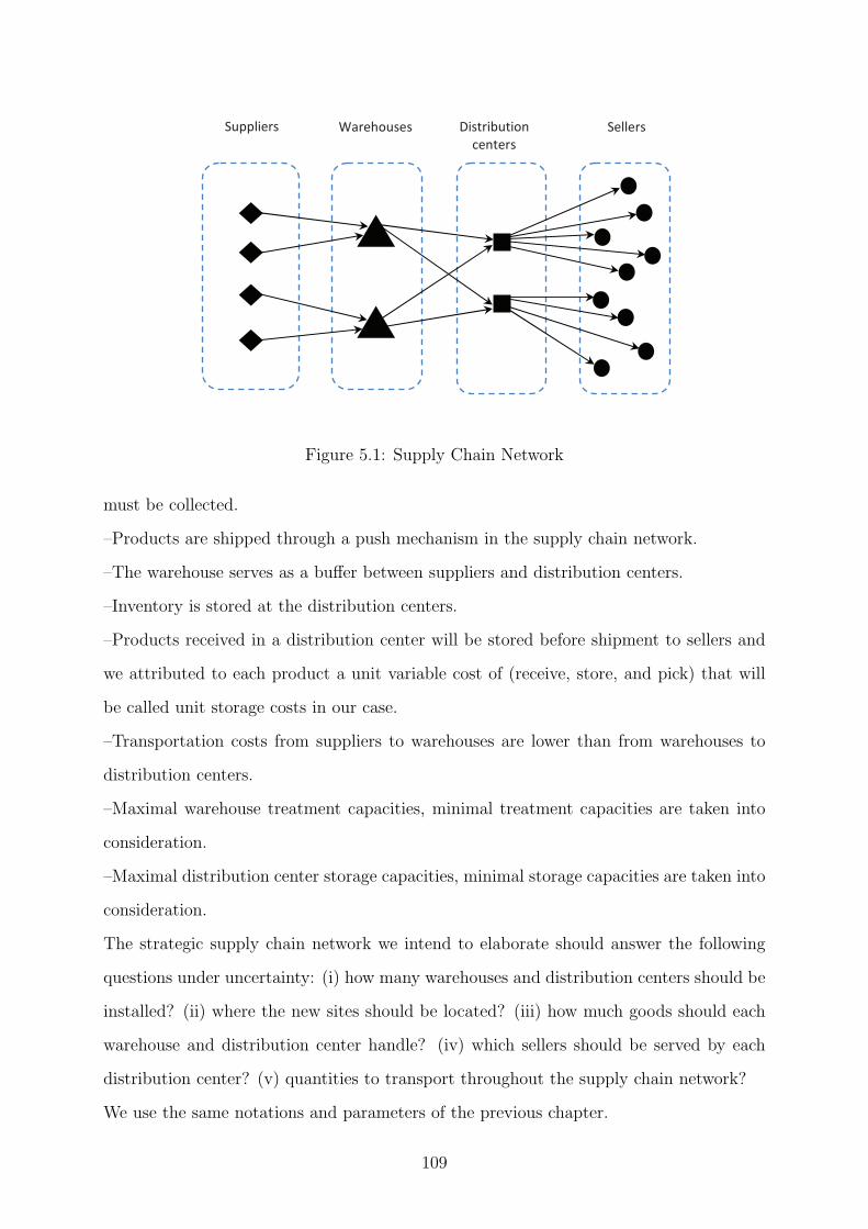
��������� ��������� �������� �
�� ���
�������
Figure 5.1: Supply Chain Network
must be collected.
–Products are shipped through a push mechanism in the supply chain network.
–The warehouse serves as a buffer between suppliers and distribution centers.
–Inventory is stored at the distribution centers.
–Products received in a distribution center will be stored before shipment to sellers and
we attributed to each product a unit variable cost of (receive, store, and pick) that will
be called unit storage costs in our case.
–Transportation costs from suppliers to warehouses are lower than from warehouses to
distribution centers.
–Maximal warehouse treatment capacities, minimal treatment capacities are taken into
consideration.
–Maximal distribution center storage capacities, minimal storage capacities are taken into
consideration.
The strategic supply chain network we intend to elaborate should answer the following
questions under uncertainty: (i) how many warehouses and distribution centers should be
installed? (ii) where the new sites should be located? (iii) how much goods should each
warehouse and distribution center handle? (iv) which sellers should be served by each
distribution center? (v) quantities to transport throughout the supply chain network?
We use the same notations and parameters of the previous chapter.
109

The total cost (5.1) is composed of fixed warehouse opening costs, fixed distribution cen-
- Numbers:
m number of supplier locations.
n number of possible warehouse locations.
p number of possible distribution center locations.
q number of customer locations.
- Indices :
i supplier index.
j possible warehouse location indices.
k possible distribution center location indices.
l customer index.
- Parameters :
Ai capacity of supplier i.
fcj fixed cost of opening warehouse j.
fj processing costs at warehouse j.
Fmaxj maximum processing capacity at warehouse j.
Fminj minimum processing capacity at warehouse j.
dck fixed cost of opening distribution center k.
ck storage costs at distribution center k.
Cmaxk maximum storage capacity of distribution center k.
Cmink minimum storage capacity of distribution center k.
µij unit transportation costs of goods between supplier i and warehouse j.
µjk unit transportation costs of goods between warehouse j and distribution center k.
µkl unit transportation costs of goods between distribution center k and customer l.
ter opening costs, transportation costs of goods throughout the supply chain, production
and storage costs. They are calculated in equation (5.1) as follows:
Minimize
[
∑
j∈W
(fcj · xj) +∑
k∈D
(dck · yk) +∑
i∈S
∑
j∈W
(µij + fj) · qij +
∑
i∈S
∑
k∈D
(µik + ck) · qik +∑
j∈W
∑
k∈D
(µjk + ck) · qjk +∑
k∈D
∑
l∈C
µkl · qkl
]
(5.1)
110

µik unit transportation costs of goods between supplier i and distribution center k.
Dl demand of the customer l.
- Decision variables:
xj =1 if warehouse j is opened, and = 0 otherwise.
yk =1 if distribution center k is opened, and = 0 otherwise.
qij quantity of products transported from supplier i to warehouse j.
qjk quantity of products transported from warehouse j to distribution center k.
qkl quantity of products transported from distribution center k to customer l.
qik quantity of products transported from supplier i to distribution center k.
Subject to
Constraint (5.2) imposes that all goods received by suppliers will be transported to ware-
house:
∑
j∈W
qij +∑
k∈D
qik = Ai i ∈ S. (5.2)
Constraint (5.3) enforces the flow conservation of products in warehouses level:
∑
i∈S
qij =∑
k∈D
qjk j ∈ W. (5.3)
Constraint (5.4) limits the warehouse treatment capacity :
Fminj · xj ≤
∑
i∈S
qij ≤ Fmaxj · xj j ∈ W. (5.4)
Constraint (5.5) enforces flows conservation of products in distribution centers level:
∑
j∈W
qjk+∑
i∈S
qik =∑
l∈C
qkl k ∈ D. (5.5)
Constraint (5.6) limits the distribution center capacity:
Cmink ·yk ≤
∑
j∈W
qjk+∑
i∈S
qik ≤ Cmaxk ·yk k ∈ D. (5.6)
Constraint (5.7) guarantees that customer’s demand will be satisfied:
∑
k∈D
qkl = Dl l ∈ D. (5.7)
111

Constraints (5.8), and (5.9) enforce the binary nature of xj and yk :
xj ∈ {0, 1} j ∈ W. (5.8)
yk ∈ {0, 1} k ∈ D. (5.9)
Constraints (5.10), (5.11), (5.12) et (5.13) are standard non-negative constraints:
qij ≥ 0 i ∈ S; j ∈ W. (5.10)
qjk ≥ 0 j ∈ W ; k ∈ D. (5.11)
qkl ≥ 0 k ∈ D; l ∈ C. (5.12)
qik ≥ 0 i ∈ S; k ∈ D. (5.13)
For example, in Table 5.1, where Exp represents instances, S denotes le suppliers num-
ber, W is the warehouses number, DC represents the distribution centers number and
C denotes customers number. To solve a SCND problem with 11 suppliers, 40 potential
Table 5.1: Global MILP model limits
Exp S W DC C Constraints Variables CPU Time (s)
D1 11 10 10 10 732 641 0.22
D6 11 10 10 103 1755 1571 3.58
D7 11 16 20 103 3701 3469 51.59
D10 11 40 63 103 16248 15815 36232
D13 11 100 100 103 46510 45761 16012
D15 11 140 140 140 82762 81761 OM*
D16 11 160 160 160 107385 106241 OM*
*OM: Out of Memory
warehouses, 63 potential distribution centers and 103 customers using an exact method,
we need 36 232 seconds to find the solution. Also, our computational experiences show
that it’s impossible to solve SCND problems using an exact method implemented on com-
mercial solver like Cplex. Limits of the MILP model are recapitulated on Table 5.1. This
is far of our objective, which is to solve a large scale application case with 1500 customers,
220 potential distribution centers, 220 potential warehouses and 220 suppliers.
In the following section, the heuristic algorithm based on decomposition technique is
presented.
112

5.3 Heuristic Approach
In this section, we present a heuristic approach to solve the global supply chain problem.
Our aim is to obtain good solutions for large scale SCND problems in a reasonable time.
The core idea behind the heuristic method is to reduce each facilities set of the original
supply chain network as small set. The network is then reduced to a medium size problem
that could be solved using an exact method.
We build the heuristic on ideas developed in two works. We integrate the concept of
decomposition as discussed in Cheng and Wang (2009), the idea of their heuristic de-
composition procedure is to divide the large-scale global distribution into some identified
sub-problems such as: facility location problem, location-allocation problem, hub location
problem, transportation problem, travelling salesman problem, vehicle routing problem,
etc. Then, each sub-problem is solved and the global solution is the sum of all these
solutions.
We also use the concept of decomposition of the entire supply chain network as discussed
in Jang et al. (2002), they decomposed the entire SCN into three sub-networks: The
inbound sub-problem consists of all suppliers to the manufacturing plants, the distribu-
tion sub-problem includes facilities where the final products are manufactured and the
distribution facilities, the outbound sub-network consists of customers and distributors
close to customers. They used the Lagrangian relaxation to solve each sub-network.
To determine the reduced supply chain network of the original huge one presented in
Figure 5.2, it is first decomposed into two-level sub-problems. Then, the well-known p-
median model (Klose and Drexl (2005) and ReVelle et al. (2008)) is used to solve each
sub-problem. Finally the reduced supply chain network is solved using the global MILP
model (5.1)-(5.13). The heuristic are detailed in the following subsections.
5.3.1 Heuristic Structure
The heuristic approach consists of three phases as follows:
Phase 1: Decomposition phase : in this phase we decompose the huge supply chain
network into small sub-networks with decomposition technique. The decomposition pro-
cess continues until the problem is divided into two levels sub-problems that we can solve
113
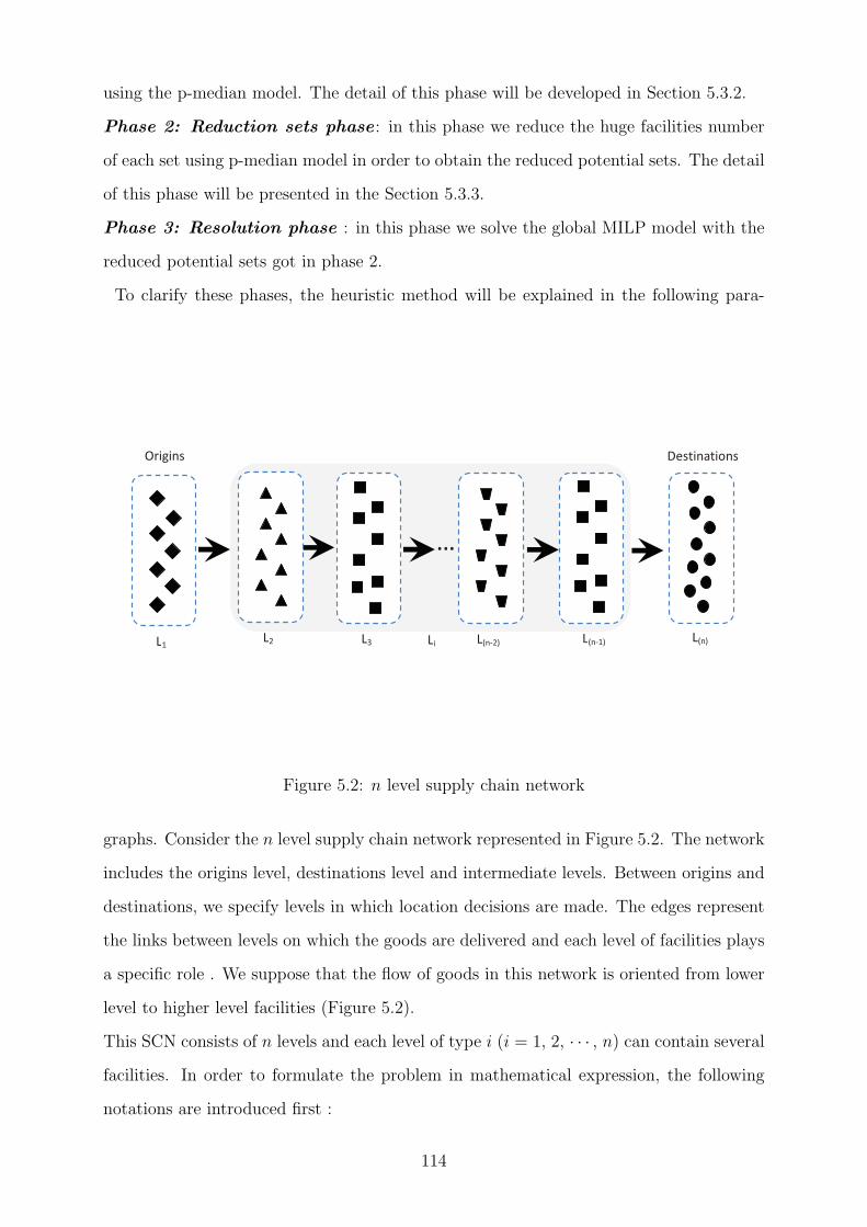
using the p-median model. The detail of this phase will be developed in Section 5.3.2.
Phase 2: Reduction sets phase : in this phase we reduce the huge facilities number
of each set using p-median model in order to obtain the reduced potential sets. The detail
of this phase will be presented in the Section 5.3.3.
Phase 3: Resolution phase : in this phase we solve the global MILP model with the
reduced potential sets got in phase 2.
To clarify these phases, the heuristic method will be explained in the following para-
������ ��� ������
��� ����
�
��
�������������
�����
������
��
Figure 5.2: n level supply chain network
graphs. Consider the n level supply chain network represented in Figure 5.2. The network
includes the origins level, destinations level and intermediate levels. Between origins and
destinations, we specify levels in which location decisions are made. The edges represent
the links between levels on which the goods are delivered and each level of facilities plays
a specific role . We suppose that the flow of goods in this network is oriented from lower
level to higher level facilities (Figure 5.2).
This SCN consists of n levels and each level of type i (i = 1, 2, · · · , n) can contain several
facilities. In order to formulate the problem in mathematical expression, the following
notations are introduced first :
114
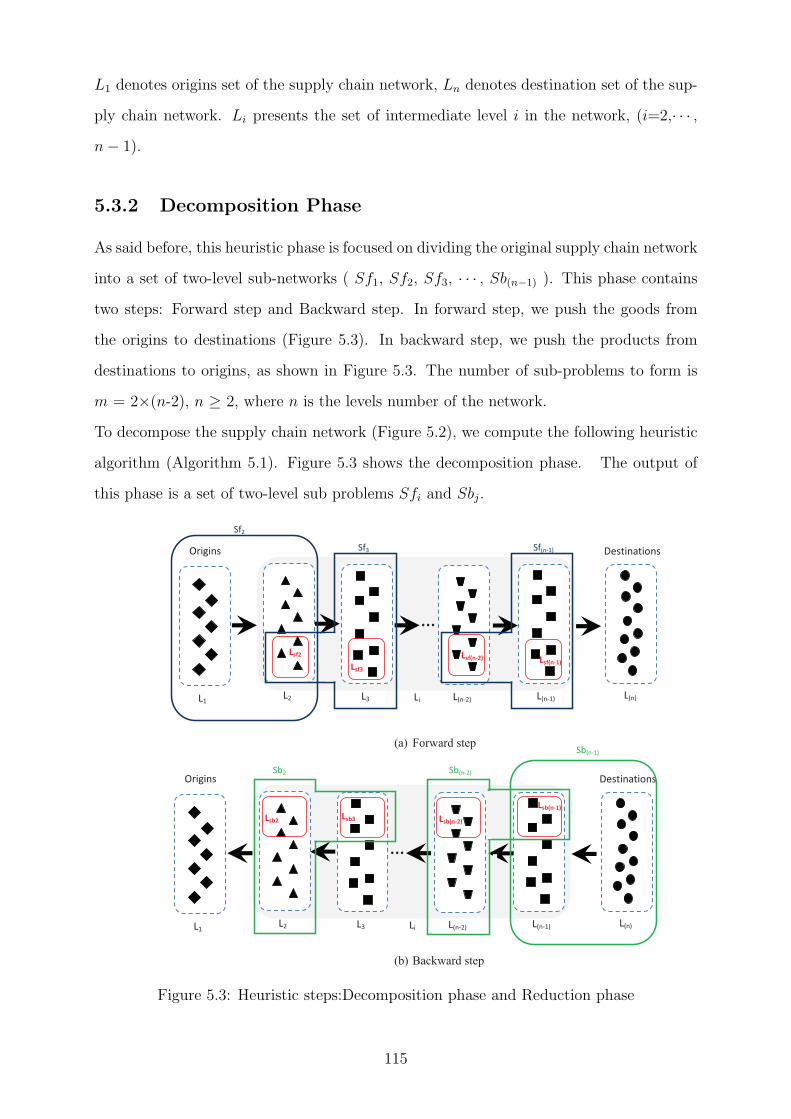
L1 denotes origins set of the supply chain network, Ln denotes destination set of the sup-
ply chain network. Li presents the set of intermediate level i in the network, (i=2,· · · ,
n− 1).
5.3.2 Decomposition Phase
As said before, this heuristic phase is focused on dividing the original supply chain network
into a set of two-level sub-networks ( Sf1, Sf2, Sf3, · · · , Sb(n−1) ). This phase contains
two steps: Forward step and Backward step. In forward step, we push the goods from
the origins to destinations (Figure 5.3). In backward step, we push the products from
destinations to origins, as shown in Figure 5.3. The number of sub-problems to form is
m = 2×(n-2), n ≥ 2, where n is the levels number of the network.
To decompose the supply chain network (Figure 5.2), we compute the following heuristic
algorithm (Algorithm 5.1). Figure 5.3 shows the decomposition phase. The output of
this phase is a set of two-level sub problems Sfi and Sbj.
(a) Forward step �
�
�
�
�
�
�
�
�
�
�
�
�
�
�
(b) Backward step �
������ ��� ����� �
�
!������
�
���
� ���������
��� �
������ �
����
���� ������ �
����
����
�������� ��������
������ ��� ����� �
�
!������
�
���
� ���������
��� �
������ �
"�
"�
��������
�������� ���� ����
������ �
������ �����
Figure 5.3: Heuristic steps:Decomposition phase and Reduction phase
115

Algorithm 5.1: DECOMPOSITION ALGORITHM
Input:
Li: set of level i in the supply chain network.
Output:
Sf : forward sub-problems.
Sb: backward sub-problems.
1 begin
2 /* Forward Step*/
3 for (i = 1 to i = n− 2) do
4 if (i = 1) then
5 Sf(2) ←− {L1, L2}
6 Sf(i+1) ←− {LSf(i) , L(i+1)}
7 /* Backward Step*/
8 for (j = n to j = 3) do
9 if (j = n) then
10 Sb(n−1) ←− {Ln, L(n−1)}
11 Sb(j−1) ←− {LSb(j) , L(j−1)}
12 Return (Sf, Sb)
5.3.3 Reduction Phase
We compute reduction algorithm (Algorithm 5.2) for each sub-problem Sfi and Sbi, in
order to reduce the size of each potential set Li to new reduced set Lri.
The idea of this step, is to keep the same costs or criteria used in the objective function of
the global MILP model to locate warehouses ans distribution centers. This means that, to
reduce the warehouses set, we integrate in the objective function of the p-median problem
warehouse opening costs, production costs and transportation costs, because these costs
are used in the global MIPL model to locate warehouses. Also, to reduce the distribution
centers set, the objective function of the p-median problem contains distribution center
opening costs, storage costs and transportation costs.
In order to calculate the p value, we solve the largest MILP model composed of suppliers
116

Algorithm 5.2: REDACTION ALGORITHM
Input:
Sf : forward sub-problems.
Sb: backward sub-problems.
Output:
LSf : reduced set of forward sub-problems.
LSb: reduced set of backward sub-problems.
Lr: reduced set.
1 begin
2 /* Forward Step*/
3 for (i = 1 to i = (n− 2)) do
4 LSf(i+1)←− p−median(Sf(i+1))
5 /* Backward Step*/
6 for (j = n to j = 3) do
7 LSb(j−1)←− p−median(Sb(j−1))
8 /* Reduced Sets*/
9 for (i = 2 to i = (n− 1)) do
10 Lri ←− LSf(i) ∪ LSb(i)
11 Return (LSf , LSb, Lr)
set, p warehouses, p distribution centers and customers set, that we can solve using the
commercial software Cplex.
A general p-median problem involves a set of customers and a set of facilities to serve
customer demands (see Drezner and Hachamer (2004), ReVelle and Eiselt (2005), Klose
and Drexl (2005) and ReVelle et al. (2008)).
Let us define parameters and variables of the p-median model (Figure 5.4): S represents
suppliers set and W is potential facilities set. p denotes the number of facilities to open,
fj represents fixed cost of opening facility at candidate node j, cj denotes unit cost of
production goods at candidate facility j, µij is the unit transportation costs of goods
between node i and node j, di denotes quantities supplied by supplier i. Xj =1 if we
117

���������
��
��� ����
����������
����
���������
Figure 5.4: p-median network
locate facility at candidate site j, and = 0 else. Yij =1 if goods quantities at node i are
received by a facility at candidate site j, and = 0 else.
Minimize∑
j∈W
(fj ·Xj) +∑
j∈W
∑
i∈S
(µij + cj) · di · Yij (5.14)
Subject to
Constraint (5.15) requires that exactly p facilities be located:
∑
j∈W
Xj = p (5.15)
Constraint (5.16) ensures that every demand is assigned to some facility site:
∑
i∈S
Yij = 1 j ∈ W. (5.16)
Constraint (5.17) allows assignment only to sites at which facilities have been located:
Yij −Xj ≤ 0 i ∈ S; j ∈ W. (5.17)
Constraints (5.18) and (5.19) are standard non-negative and integrity constraints:
Xj ∈ {0, 1} j ∈ W. (5.18)
Yij ∈ {0, 1} i ∈ S; j ∈ W. (5.19)
5.3.4 Resolution Phase
After the resolution of the previous two phases, the supply chain network system is reduced
in complexity to the original SCN, due to reduction of the size of the potential sets to
small size sets. In this phase, we solve the reduced supply chain network problem using
the global MILP model (5.1)-(5.13).
118

5.4 Application Case
In this section, we apply the proposed heuristic approach to our application case, as shown
in Figure 5.5. We consider a real life supply chain network consists of 220 suppliers, 220
potential warehouse locations, 220 potential distribution center locations , and 1500 sellers
. In order to describe the supply chain network (Figure 5.5), we define notations as follows:
�
������ �� �� ���� �� ����������
� � ��
� �� ��
��� ��� ��� ���
Figure 5.5: Supply Chain Network
we let L1 denotes suppliers set and L2 denotes warehouses set, L3 presents distribution
centers set, L4 is customers set.
5.4.1 Decomposition Phase
To find a feasible solution for the SCND problem, we start by dividing the problem
into four sub-problems: suppliers-warehouses sub-problem Sf2={L1,L2} (see Figure 5.6
(a)), warehouses-distribution centers sub-problem Sf3={LSf2 ,L3} (see Figure 5.6 (b)),
customers-distribution centers sub-problem Sb3={L4,L3} (see Figure 5.6 (c)) and distri-
bution centers-warehouses sub-problem Sb2={LSb3 ,L2} (see Figure 5.6 (d)).
As illustrated in Figure 5.6. Where LSf2 is the first potential warehouses set obtained
solving sub-problem Sf2. LSb3 denotes second potential distribution centers set obtained
solving sub-problem Sb3.
119

(a) (b)
Forward step
(c) (d)
Backward step
��� ���
��� ���
�����
���
���
����
����
����
����
����
Figure 5.6: Decomposition phase
5.4.2 Reduction Phase
To reduce the huge size of the potential sets of the SCN, p-median model should be run
for each sub-problem. In order to calculate the p value, we solve the largest MILP model
composed of 220 suppliers, p warehouses, p distribution centers and 1500 customers. We
find that p is equal to 14.
For this case, the reduction phase contains four steps as presented in Figure 6.2, which
represent the number of sub-problem obtained in the previous phase. How this reduction
can be achieved will be explained in the following steps.
Step 1
In this step, we apply the p-median model to the first sub-problem Sf2 obtained in the
decomposition phase. As we can see on Figure 5.8, the detail of this step, the sub-
problem Sf2 is composed of two sets: suppliers set L1 and warehouses set L2. To get the
first potential warehouses set LSf2 , we solve the following mathematical model (5.20). In
addition to parameters and variables defined in previous section, let’s introduce those of
120

�
������ ������ ������
����� �����
Figure 5.7: Heuristic steps: Decomposition phase and Reduction phase
Figure 5.8: Step 1
121

the p-median model: p denotes the number of warehouses to open, which is equal to 7 in
this step. di denotes quantities shipped from the supplier i. Xj =1 if we locate warehouse
at candidate site j, and = 0 else. Yij =1 if goods at node i are served by a warehouse at
candidate site i, and = 0 else.
Minimize∑
j∈L2
(fcj ·Xj) +∑
i∈L1
∑
j∈L2
(µij + fj) · di · Yij (5.20)
Subject to
(5.15), (5.16), (5.17), (5.18), (5.19).
The output of this step is the first potential warehouses set LSf1 that we will use in step
4.
Step 2
In this step, we try to reduce potential distribution centers set L3. However, we solve the
p-median problem applied to the second sub-problem Sf3 obtained in the decomposition
phase. Figure 5.9 outlines the detail of this step, the sub-problem Sf3 is composed of two
sets: first potential warehouses set distribution centers set LSf2 and distribution centers
set L3. Parameters and variables used in the p-median model: p denotes the number
Figure 5.9: Step 2
of potential distribution centers to open. di denotes quantities supplied from warehouse
i. Xj =1 if we locate distribution center at candidate site j, and = 0 else. Yij =1 if
distribution center j are served by a warehouse at candidate site i, and = 0 else.
122

Minimize∑
j∈L3
(dcj ·Xj) +∑
i∈LSf2
∑
j∈L3
(µij + cj) · di · Yij (5.21)
Subject to
(5.15), (5.16), (5.17), (5.18), (5.19).
We fix the number of potential distribution centers to open p = 7, then we solve the
model. The output of this step is the first potential distribution centers set LSf3 that we
will use in step 3.
Step 3
Figure 5.10 outlines the detail of this step. The sub-problem Sb3 contains two sets: the
first potential warehouses set LSb1 and distribution centers set L3. First, we fix the number
of potential distribution centers to open p to 7. Then, we solve the following p-median
problem (5.22) applied to Sb3 sub-problem in order to get the second potential distribution
centers set LSb3 . Before presenting the objective function of the p-median problem, let’s
Figure 5.10: Step 3
define parameters and variables of this model: di denotes demand of customer i. Xj =1
if we locate distribution center at candidate site j, and = 0 else. Yij =1 if demand at
customer i are served by distribution center at candidate site j, and = 0 else.
Minimize∑
j∈L4
(fcj ·Xj) +∑
i∈L4
∑
j∈L3
(µij + fj) · di · Yij (5.22)
Subject to
(5.15), (5.16), (5.17), (5.18), (5.19).
123

Outputs of this step are the second potential distribution centers set LSb3 and Lr3= LSf3
∪ LSb3 that we will use in step 5.
Step 4
In this step, the sub-problem Sb2 contains two sets: first potential distribution center set
LSb3 and warehouses set L2 (Figure 5.11). In order to get the second potential warehouses
set LSb2 . We solve the p-median problem applied to this sub-problem
Parameters and variables of this model are: p denotes the number of potential distribution
Figure 5.11: Step 4
centers to open, p = 7 in this step. di denotes quantities supplied from warehouse i. Xj
=1 if we locate warehouse at candidate site j, and = 0 else. Yij =1 if warehouse j are
served by a distribution center at candidate site i, and = 0 else.
Minimize∑
j∈L2
(dcj ·Xj) +∑
i∈LSb3
∑
j∈L2
(µij + cj) · di · Yij (5.23)
Subject to
(5.15), (5.16), (5.17), (5.18), (5.19).
Outputs of this step are the second potential warehouses set LSb2 and Lr2= LSf2 ∪ LSb2
that we will use in step 5.
5.4.3 Resolution Phase
Now, we have the reduced supply chain network. As we can see on Figure 5.12, this
network is composed of : suppliers set A, reduced potential warehouses set Lr2={LSf2 ∪
124

LSb2}, reduced potential distribution centers set Lr3={LSf3 ∪ LSb3} and customers set D.
We solve the MILP model (5.1)-(5.13) in order to find the optimal supply chain network
solution.
Figure 5.12: Step 5
5.5 Computational Results
In this section we describe numerical experiments using the heuristic algorithm for solving
real case supply chain design problem. We first explain instances and some implementa-
tion details. Then, we highlight the computational efficiencies of our heuristic method.
Finally, we outline the quality of the heuristic solutions in comparison to those obtained
using a MILP model.
5.5.1 Data and Implementation
We consider a real life supply chain network. Our case consists of 220 suppliers, 220
potential warehouse locations, 220 potential distribution center locations , and 1500 sellers
that the company serves. We generated 26 test problems from this real life SCN, to
evaluate the performance of the heuristic methodology and the global MILP model (5.1)-
(5.13). This means that, we reduced randomly the size of customers set from 1500 to
10 customers, the size of distribution centers set from 220 to 10 distribution centers,
warehouses number from 220 elements to 10 warehouses and the size of suppliers set from
220 suppliers to 11 suppliers (Table 5.2).
These instances are complemented on Windows Vista 1.66 GHZ and 2 GB of memory
125

and solved by commercial software ILOG OPL 6.3/ CPLEX 12.1.0 (ILOG (2011)).
To solve the Global MILP of some large instances, from instance D15 to instance D26,
we used some specific cuts in order to speed up the resolution (see Paquet et al. (2004)).
Cuts proposed for the model presented here are related to numbers of distribution centres
and warehouses to open. They are defined by equations (5.24) to (5.25). Equation (5.24)
calculates the maximum number of warehouses to open and Equation (5.25) ensures that
the maximum number of distribution centers to open is equal to 4.
∑
j∈W
xj ≤ 2 (5.24)
∑
k∈D
yk ≤ 4 (5.25)
The main characteristics of this SC networks are presented in Chapter 3.
5.5.2 Performance of Heuristic
In this subsection, we discuss the performance of the heuristic algorithm for solving SCND
problems. To measure this performance, we select the following performance indicators:
(i) constraints number; (ii) variables number; (iii) CPU Time.
Constraints number and variables number of the heuristic method obtained solving the
last phase of the approach. The CPU Time of the heuristic presents the addition of the
computational times of all heuristic phases.
Table 5.2 summarizes results of the two approaches global MILP and heuristic.
Results are described by providing suppliers number (S), the potential warehouse sites
number (W), the potential distribution centers number (DC), the constraints number and
variables number.
Table 5.2 reveals that the global MILP model contains more constraints and variables
than the heuristic approach. As we can see, for small instances, from D1 to D6, vari-
ables and constraints number of both models are in the same number level, because the
number of facilities in warehouses set and distribution centers set are static equal to 10.
Increasing the number of facilities in these sets, the difference in number of constraints
and variables between two models go up. For example, for D20 we find that constraints
number is equal to 288 404 and 5 964 using MILP model and heuristic respectively.
126

�������
�������
�������
�������
�������
������������� �
�
������
�������
�� �� �� �� �� � � �� �� ��� ��� ��� ��� ��� ��� �� �� ��� ��� ���
��
������� �
� � �������������������� � ����������������
Figure 5.13: Constraints: MILP model vs Heuristic
It is clear that, the use of heuristic method help us to decrease the complexity of the
problem by reducing constraints and variables number. Figure 5.13 shows the increase of
constraints number of MILP model with the growth of the sample size. We compare the
constraints number required for solving a MIL problem to the heuristic, for each experi-
ence. As we can see, the constraints number using MILP model goes up exponentially
with the increase of the instance size, while it increases slowly with the network size using
our heuristic.
Figure 5.14 depicts the increase of variables number of MILP model with the growth
of instance size. We compare the variables number required for solving MILP using
commercial solver to the heuristic, for each experience. It’s clear that using our heuristic,
increasing the instance size the variables number rises from 650 to 5 500 (Table 5.2), while
it rises exponentially ( from 641 to 238 481) with the increase of the instance size using the
global MILP model. Figure 5.15 charts the increase of the computational time with the
growth of the sample size. For each instance, we compare the CPU seconds required for
solving the MILP model to the heuristic algorithm proposed in Section 5.2. The efficacy
of the proposed heuristic is clearly observed. For more detail you can refer to Table 6.8.
127

�������
�������
�������
�������
��������������
�
������
�������
�� �� �� �� �� � � �� �� ��� ��� ��� ��� ��� ��� �� �� ��� ��� ���
������
��������������������� ������������������
Figure 5.14: Variables: MILP model vs Heuristic
������
������
������
������
������
������
������
�������
���
�
�����
�����
������
� � �� �� �� �� �� �� �� �� � � �� �� �� �� �� �� �� ��
� �� ��
������� ��������������� �������������������
Figure 5.15: CPU time: MILP model vs Heuristic
128
Table 5.2 reveals that solutions of the heuristic approach are not only superior to MILP
solution in terms of the CPU time, but these solutions also lead to smaller number of
constraints and variables.
The computational experimentation compares performances of the proposed heuristic
approach and the MILP approach. Limited computational results show that although
the latter is more effective in solving smaller-sized test instances, the proposed heuristic
approach appears to be more promising for larger test instances.
The quality of heuristic solutions are presented in the following subsection.
5.5.3 Quality of Heuristic Solutions
In this section we compare solutions of the heuristic algorithm to that of MILP model
using the following performance indicators: (i) costs; (ii) Gap; (iii) SC configuration.
- Costs: refers to the sum of all costs that are generated : opening costs, processing costs,
storage and transportation costs.
- Gap: refers to the percentage of cost difference between solutions.
Gap 1 =
(
Heuristic costs−Global MILP costs
Global MILP costs
)
× 100 (5.26)
Gap 2 =
(
Heuristic costs− Lower bound
Lower bound
)
× 100 (5.27)
Where Global MIPL costs represents the objective function value obtained solving the
global MILP. The Heuristic costs is the objective function value of the last step of the
heuristic method. The Lower bound represents the lower bound value of the global MILP
calculated by solver Cplex.
- SC configuration: refers to the supply chain network structure proposed by the mathe-
matical model.
In Table 6.8, we compare the solution obtained from the heuristic algorithm with the
global MILP solution that we got using Cplex solver. We first solve small size instances,
from D1 to D7, we find that the gap between the heuristic solution and the global MILP
solution (Gap 1), for all these instances, is equal to zero percent. We conclude that using
our heuristic, we can establish optimal solution to small sized problems, with an excel-
lent quality. Then, we conduct further experiments to test the heuristic for medium size
129

Table 5.2: Constraints and variables numbers: Heuristic vs Global MILP model
MILP Model Heuristic
Exp S W DC C Constraints Variables Constraints Variables
D1 11 10 10 10 732 641 732 641
D2 11 10 10 20 842 741 576 490
D3 11 10 10 40 1062 941 854 742
D4 11 10 10 60 1282 1141 1034 902
D5 11 10 10 80 1502 1341 1214 1062
D6 11 10 10 103 1755 1571 1421 1246
D7 11 16 20 103 3701 3469 2465 2263
D8 11 16 40 103 7581 7289 1859 1675
D9 11 16 63 103 13032 12671 2208 2015
D10 11 40 63 103 16248 15815 1965 1781
D11 11 63 63 103 20411 19909 1859 1675
D12 11 80 80 103 30046 29441 2166 1969
D13 11 100 100 103 46510 45761 2166 1969
D14 11 120 120 120 61342 60481 2546 2330
D15 11 140 140 140 82762 81761 2444 2214
D16 11 160 160 160 107385 106241 3106 2850
D17 11 180 180 180 135202 133921 3335 3062
D18 11 200 200 200 206024 164801 3414 3121
D19 11 220 220 220 248624 198881 4330 4005
D20 11 220 220 400 288404 238481 5964 5474
D21 11 220 220 600 - - 7964 7274
D22 11 220 220 800 - - 10315 9428
D23 11 220 220 1000 - - 12715 11628
D24 50 220 220 1200 - - 17428 16057
D25 100 220 220 1500 - - 24411 22634
D26 220 220 220 1500 - - 18724 16725
130

Table 5.3: CPU time: Heuristic vs Global MILP model
Exp S W DC C MILP Model CPU Time (s) Heuristic CPU Time (s)
D1 11 10 10 10 0.22 0.23
D2 11 10 10 20 0.28 0.53
D3 11 10 10 40 1.12 1.94
D4 11 10 10 60 2.2 2.42
D5 11 10 10 80 2.14 2.12
D6 11 10 10 103 3.58 2.06
D7 11 16 20 103 51.59 22.34
D8 11 16 40 103 3482 32.26
D9 11 16 63 103 44777 36.44
D10 11 40 63 103 36232 10.39
D11 11 63 63 103 87548 16
D12 11 80 80 103 8536 22
D13 11 100 100 103 16012 28
D14 11 120 120 120 9822 18
D15 11 140 140 140 81000* 21
D16 11 160 160 160 81000* 31
D17 11 180 180 180 81000* 33
D18 11 200 200 200 81000* 35
D19 11 220 220 220 81000* 43
D20 11 220 220 400 81000* 22
D21 11 220 220 600 - 38
D22 11 220 220 800 - 50
D23 11 220 220 1000 - 76
D24 50 220 220 1200 - 125
D25 100 220 220 1500 - 350
D26 220 220 220 1500 - 550
131

problems (D8 to D14). As we can see on Table 6.8, the Gap 1 for these problems ranges
from 0% to 0.52%. To test the heuristic algorithm for large size problems, we increased
suppliers number from 11 to 220, warehouses number from 120 to 220, distribution centers
from 120 to 220 and customers number from 120 to 1 500. In these cases, the heuristic
was able to find solutions in reasonable time. In contrast to the global MILP model that
did not succeed to obtain any solution. The Gap 1 was impossible to calculate, because
we didn’t succeed to solve the problem using the exact MILP model. However, we will use
Gap 2 to compare large size problems. The Gap between the best integer and the heuris-
tic solution (Gap 2) ranges between 1.19% and 9.52%, the Gap 2 average is equal to 5.66%.
In Table 5.5, for instances D1 to D7, the CPU time varied significantly. The time
spent to get the solution by the global MILP model using the solver is at least 10 times
more than the time passed by heuristic approach. For these instances, the supply chain
configurations proposed by the global MILP model and the heuristic are exactly the same.
For example, the SC configuration obtained solving instance D4 using the global MILP
model is: two distribution centres {CD13,CD35} and one warehouse {F35}. We got the
same SC configuration using our heuristic to solve the instance D4 (Table 5.5).
It’s clear that using our heuristic, we can establish optimal solution to small sized prob-
lems, in a reasonable time, even faster than the global MILP model and the quality of
the solution is equal to the global model one.
Then, the computing times using the heuristic to solve medium size instances (D8 to
D14), are largely better than those using the global MILP. For example, the time that
the global MILP model took to solve the problem D9 is equal to 44 777 seconds , while
for the same problem the heuristic took only 37 seconds to get the optimal solution. Also,
for instances D8 to D14, the SC configurations of the both approaches are equals or a
small difference in one distribution center like in D10, the SC configuration proposed
by the global MILP model is {CD35, CD96, CD137, CD49} as distribution centers
and {F137} as warehouse, the SC configuration established by the heuristic algorithm is
{CD35, CD96, CD137, CD219} as distribution centers and {F137} as warehouse.
For experiments D15 to D26, as we can see on Table 5.7, Table 5.8 and Table 5.9, it’s
impossible to solve these instances using global MILP model, all of them are out of mem-
132

ory (OM). But, using our heuristic we succeeded to obtain solutions in reasonable time.
Finally, Tables 5.5, 5.6, 5.7, 5.8, 5.9 and 5.10 show the SC configuration and computing
time obtained solving 26 instances using the heuristic algorithm and the global MILP
model.
Table 5.4: Solutions: Heuristic vs Global MILP model
Exp MILP costs (e) Lower bound(e) Heuristic costs (e) Gap 1 (%) Gap 2 (%)
D1 50 969 501 - 50 969 501 0,00% -
D2 49 104 009 - 49 104 009 0,00% -
D3 63 190 371 - 63 190 371 0,00% -
D4 64 479 173 - 64 479 173 0,00% -
D5 64 862 948 - 64 862 948 0,00% -
D6 66 583 537 - 66 583 537 0,00% -
D7 66 583 537 - 66 583 537 0,00% -
D8 60 864 271 - 60 864 271 0,00% -
D9 60 846 506 - 61 053 982 0,34% -
D10 58 253 135 - 58 554 399 0,52% -
D11 58 253 135 - 58 554 399 0,52% -
D12 59 366 319 - 59 591 091 0,38% -
D13 59 197 681 - 59 366 319 0,28% -
D14 47 546 627 - 47 546 627 0,00% -
D15 - 49 077 542 49 659 208 - 1,19%
D16 - 47 518 700 48 390 006 - 1,83%
D17 - 48 255 402 49 807 395 - 3,22%
D18 - 47 738 700 51 964 143 - 8,85%
D19 - 46 192 400 50 588 271 - 9,52%
D20 - 47 549 019 52 010 862 - 9,38%
Average 0,15% 5,66%
133

Table 5.5: Configuration: Heuristic vs Global MILP (Part 1)
Global MILP Model Heuristic
Exp CPU Time (s) CD and capacities W and capacities CPU Time (s) CD and capacities W and capaci-
ties
D1 0,22 CD35(10000000);
CD39(115160000)
F35(125160000) 0,23 CD35(10000000);
CD39(115160000)
F35(125160000)
D2 0,28 CD35(45405000);
CD39(79753000)
F35(125160000) 0,53 CD35(45405000);
CD39(79753000)
F35(125160000)
D3 1,12 CD8(26596000);
CD35(98562000)
F35(125160000) 1,94 CD8(26596000);
CD35(98562000)
F35(125160000)
D4 2,2 CD13(84790000);
CD35(40368000)
F13(125160000) 2,42 CD13(84790000);
CD35(40368000)
F13(125160000)
D5 2,14 CD13(16006000);
CD8(44538000);
CD35(64555000)
F35(125160000) 2,12 CD13(16006000);
CD8(44538000);
CD35(64555000)
F35(125160000)
D6 3,58 CD13(16006000);
CD35(64555000)
F35(125160000) 2,06 CD13(48877000);
CD35(76281000)
F35(125160000)
D7 51,59 CD13(48877000);
CD35(76281000)
F35(125160000) 22,34 CD13(48877000);
CD35(76281000)
F35(125160000)
134

Table 5.6: Configuration: Heuristic vs Global MILP (Part 2)
Global MILP Model Heuristic
Exp CPU Time (s) CD and capacities W and capacities CPU Time (s) CD and capacities W and capaci-
ties
D8 3482 CD35(61823000);
CD96(19152000);
CD28(44184000)
F35(125160000) 32,26 CD35(61823000);
CD96(19152000);
CD28(44184000)
F35(125160000)
D9 44777 CD35(37884000);
CD96(19152000);
CD137(41848000);
CD50(26274000)
F149(125160000) 36,44 CD35(42042000);
CD96(19152000);
CD137(44590000);
CD219(19374000)
F13(125160000)
D10 36232 CD35(38239000);
CD96(19152000);
CD137(44410000);
CD49(23357000)
F137(125160000) 10,39 CD35(38239000);
CD96(19152000);
CD137(44410000);
CD219(23357000)
F137(125160000)
D11 875487 CD35(38239000);
CD96(19152000);
CD137(44410000);
CD49(23357000)
F137(125160000) 16 CD35(38239000);
CD96(19152000);
CD137(44410000);
CD219(23357000)
F137(125160000)
135

Table 5.7: Configuration: Heuristic vs Global MILP (Part 3)
Global MILP Model Heuristic
Exp CPU Time (s) CD and capacities W and capacities CPU Time (s) CD and capacities W and capaci-
ties
D12 8536 CD3(16058000);
CD8(8409200);
CD137(51406000);
CD166(20981000);
CD171(28305000)
F149(125160000) 22 CD8(12088000);
CD137(58460000);
CD166(20981000);
CD171(33630000)
F149(125159000)
D13 16012 CD137(50424000);
CD166(20981000);
CD171(29152000);
CD89(24602000)
F149(125160000) 28 CD3(16058000);
CD8(8409200);
CD137(51406000);
CD166(20981000);
CD171(28305000)
F149(12516000)
D14 9822 CD7(27543000);
DE722(54105000);
DS513(43511000)
F66(12516000) 18 CD7(27543000);
DE722(54105000);
DS513(43511000)
F66(12516000)
D15 OM - - 21 CD8(42758000);
CD123(36330000);
CD133(46071000)
F66(12516000)
136

Table 5.8: Configuration: Heuristic vs Global MILP (Part 4)
Global MILP Model Heuristic
Exp CPU Time (s) CD and capacities W and capacities CPU Time (s) CD and capacities W and capaci-
ties
D16 OM - - 31 CD71(40843000);
CD123(29330000);
CD133(54985000)
F66(12516000)
D17 OM - - 33 CD7(27396000);
CD123(18348000);
CD134(79415000)
F66(12516000)
D18 OM - - 35 CD123(21048000);
CD134(71033000);
CD197(33077000)
F153(12516000)
D19 OM - - 43 CD8(39996000);
CD71(20421000);
CD123(16048000);
CD134(48693000)
F153(12516000)
137

Table 5.9: Configuration: Heuristic vs Global MILP (Part 5)
Global MILP Model Heuristic
Exp CPU Time (s) CD and capacities W and capacities CPU Time (s) CD and capacities W and capaci-
ties
D20 OM - - 22 CD8(39996000);
CD71(20421000);
CD123(16048000);
CD134(48693000)
F66(12516000)
D21 OM - - 38 CD8(47366000);
CD123(21277000);
CD133(53793000)
F66(12516000)
D22 OM - - 50 CD8(39687000);
CD123(26021000);
CD133(62541000)
F129(128249000)
D23 OM - - 76 CD8(25389000);
CD123(28517000);
CD133(50519000);
CD71(23353000)
F66(127778000)
D24 OM - - 125 CD8(42001000);
CD123(24830000);
CD133(48208000)
DE111(115039000)
138

Table 5.10: Configuration: Heuristic vs Global MILP (Part 6)
Global MILP Model Heuristic
Exp CPU Time (s) CD and capacities W and capacities CPU Time (s) CD and capacities W and capaci-
ties
D25 OM - - 350 CD71(34947000);
CD123(30232000);
CD134(64388000)
DEX07(83453000);
ES423(46114000)
D26 OM - - 550 CD8(40726000);
DE722(28210000);
CD123(19442000);
CD134(39197000)
DEX07(127575000)
139

5.6 Concluding Remarks
In this chapter, we have proposed a three-phase heuristic decomposition algorithm to solve
a supply chain network design problem. The heuristic consists of three phases which we
can generally define as decomposition phase, reduction phase and resolution phase. In
the decomposition phase, decomposition methods have been introduced in order to divide
the large scale of the SCN into small two-level networks. In reduction phase, a modified
p-median model has been used to reduce the large potential sets into small reduced sets.
In resolution phase, a global MILP model has been used to solve the reduced SCN.
In this chapter, we have developed a practical heuristic for large-scale supply chain net-
work design problems. We have solved a real large-scale supply chain network composed
of 220 suppliers, 220 warehouses, 220 distribution centers and 1 500 customers, in less
than 550 seconds. Computational results are generated from a set of 26 test problems.
The proposed heuristic CPU times increase almost slowly with the system size, which is
favourable for large-scale implementation. The average of heuristic CPU Time is equal
to 5 seconds for small size instances, 24 seconds for medium size problems and only 115
seconds for large scale instances. Moreover, the gap between the final solution obtained
by the proposed heuristic approach and the lower bound of global MILP obtained by
Cplex is equal to 0% in small size instances, less than 0.52% in medium size instances and
in large size problems, the gap ranges from 1.19% to 9.52% and the average gap between
the upper bound of the global MILP model and the solution of the heuristic is equal to
5.66%.
The numerical experiments have indicated that the proposed heuristic solution algorithm
performs well in terms of solution quality and computational time consumed.
Since SCND decisions are strategic and long term in nature, the influence of customers
demand in the establishment of the SCN and the effect of critical supply chain network
parameters are important. We think that it will be useful to consider the uncertainty of
these parameters, for example, by generating scenarios that capture future uncertainty of
the customers demand and costs. In this regard, the stochastic programming will be the
subject of the next chapter.
140

Chapter 6
Supply Chain Network Design under
Uncertainty
The deterministic model discussed in the previous chapter provides a base for Supply
Chain Network Design (SCND). Nevertheless, any network design obtained based on this
model, which represents the optimal deterministic configuration, has no assurance of per-
formance for any other future parameter fluctuation. Deterministic models do not handle
uncertainties and information imperfections about expected probable future business en-
vironments (Sabri et Beamon (2000), Klibi et al. (2010), Santoso et al. (2005)). As
we explained in Chapter 2, section 2.4.2, uncertainty modelling becomes an important
challenge for more realistic SCN design.
Most SCND under uncertainty researches model Supply Chain (SC) parameters uncer-
tainties with probability distributions that are usually predicted from historical data.
(Alonso-Ayuso et al. (2003), Guillen et al. (2005), Gupta and Maranas (2003), Santoso
et al. (2005)). However, whenever statistical data are unreliable, or are not even available,
stochastic models may not be the best choice (Wang and Shu (2005)). The Possibility
Theory (Zadeh (1978)) may provide an alternative which is easier and needs less data
than the Probability Theory to deal with SC uncertainties (Dubois et al. (2003)). In this
chapter, we extend the deterministic SCND model presented in chapter 5. We first assume
that we got the statistical data of the customer demands, so, we use two-stage stochastic
programming approach to model the supply chain network under demand uncertainty.
After that, we address uncertainty in all SC parameters: opening costs, production costs,
141

storage costs and customers demands. In this case, statistical data of all these parameters
are not available. However, we use possibilistic linear programming approach to model the
problem and we validate the approach in a large real case Textile supply chain network.
6.1 Stochastic Supply Chain Network Design
6.1.1 Introduction
Models discussed in the previous chapter suppose that supply chain design parameters
are deterministic. Whereas, in most cases, the future business environment under which
a supply chain network will operate is unknown and critical parameters such as customer
demands, prices, and capacities are uncertain in the real world. However, the importance
of uncertainty in supply chain design has encouraged researchers to address stochastic
parameters in supply chain design, such as Cheung and Powell (1996), Van Landeghem
and Vanmaele (2002), Yu and Li (2000).
In this part, we use two stages stochastic programming approach to model the problem.
In this approach, uncertain parameters are considered as random variables with an associ-
ated probability distribution and the decision variables are classified into two stages. The
first stage variables correspond to those decisions that need to be made first, before the
realization of the uncertainty. The second stage corresponds to those decisions made after
the uncertainty is announced. After the first stage decisions are taken and the random
events realized, the second stage decisions are subjected to the constraints imposed by
the second stage problem (Birge and Louveaux(1997)).
Santoso et al. (2005) proposed a two stage stochastic programming model and solution
algorithm for solving supply chain network design problems. Their heuristic integrates
the sample average approximation scheme with an accelerated Benders decomposition
algorithm. Authors used the proposed solution approach for solving two realistic supply
chain design problems. The first case network composed of 12 products, 6 suppliers, 17
warehouses, 8 manufacturing plants, 60 scenarios and 17 customers. The network struc-
ture of the second application case was: 13 products, 2 suppliers, 8 manufacturing plants,
60 scenarios and 238 customers. Azaron et al. (2008) developed a multi-objective stochas-
tic programming approach for supply chain design under uncertainty. They considered
142

numerous uncertain parameters such as: demands, supplies , processing, transportation,
shortage and capacity expansion costs. Authors used the goal attainment technique,
which is a variation of the goal programming technique, to solve the multi-objective
SCND problem and to generate the Pareto-optimal solutions. Computational results on
network involving 4 suppliers, 4 potential plants, 3 customers and 4 scenarios were pre-
sented. Another example of solving two-stage stochastic supply chain design problems is
Alonso Ayuso et al. (2003). The authors proposed a branch-and-fix heuristic to solve a
real problem. The networks involved 6 plants, 12 products, 24 markets, and 23 scenarios.
Two-stage stochastic supply chain network design models were proposed by MirHassani
et al. (2000), Tsiakis et al. (2001), Vila et al. (2007) and Vila et al. (2008).
As evident from the above discussion, there is a big deal of research in the supply chain
network design under uncertainty, Owen and Daskin (1998). However, research addressing
real size supply chain networks design problems is significantly small in number. Most of
the stochastic supply chain network design literature considers simplified single criterion,
single transportation mode. In addition, the existing stochastic programming approaches
for supply chain design under uncertainty are suited for a very small number of scenarios.
However, this section deals with the design of a multi-criteria, multi-level and multi-modal
supply chain network under uncertainty in order to satisfy the customers demand and to
respect the environmental, social, legislative, and economic requirements. We extend the
second step of our methodology (see chapter 3), with a stochastic mathematical model.
We validate this model on the case study concerning the recycling of sediment waterways
presented in chapter 3.
In this chapter, we look for the optimal supply chain network design to fulfil uncertain
customer demands using two-stage stochastic programming model. The objective is to
minimize the sum of: opening facilities costs, storage costs, production costs and trans-
portation costs. We determine location of treatment facilities and their capacities to
satisfy an estimated annual demand of potential customers.
The remainder of this chapter is organized as follows. Fist, we discuss the modelling
of the problem and indicate how the deterministic SCND model may be extended using
stochastic programming method. Then, the results of the stochastic programming ap-
proach are discussed in Section 6.1.3. Finally, in Section 6.1.4 some concluding remarks
143
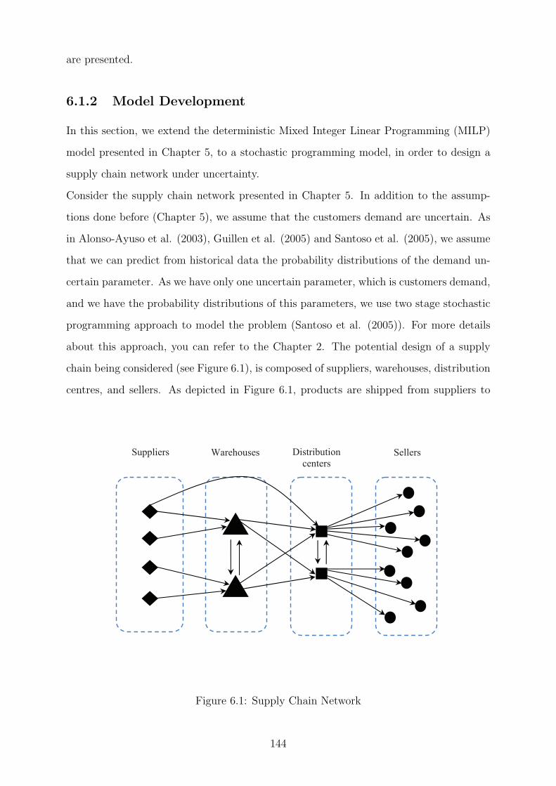
are presented.
6.1.2 Model Development
In this section, we extend the deterministic Mixed Integer Linear Programming (MILP)
model presented in Chapter 5, to a stochastic programming model, in order to design a
supply chain network under uncertainty.
Consider the supply chain network presented in Chapter 5. In addition to the assump-
tions done before (Chapter 5), we assume that the customers demand are uncertain. As
in Alonso-Ayuso et al. (2003), Guillen et al. (2005) and Santoso et al. (2005), we assume
that we can predict from historical data the probability distributions of the demand un-
certain parameter. As we have only one uncertain parameter, which is customers demand,
and we have the probability distributions of this parameters, we use two stage stochastic
programming approach to model the problem (Santoso et al. (2005)). For more details
about this approach, you can refer to the Chapter 2. The potential design of a supply
chain being considered (see Figure 6.1), is composed of suppliers, warehouses, distribution
centres, and sellers. As depicted in Figure 6.1, products are shipped from suppliers to
Suppliers Warehouses Distribution
centers Sellers
Figure 6.1: Supply Chain Network
144

warehouses, where goods are prepared to be sent to the next level. Then, they are trans-
ported to distribution centers. In some new products cases, β% of the goods should be
shipped directly to distribution centers, this percentage are fixed by experts. The distri-
bution centers insure the storage and the distribution of products to sellers. If the number
of warehouses to open is more than one site,γ% of goods received from suppliers should
be transported between warehouses in order to try to keep a quantity balance between
sites. This percentage γ are assigned by experts. Warehouses are defined as the facility
where the products are received and married with goods going to the same destination,
then shipped at the earliest opportunity, without going into long-term storage. They are
located near suppliers and distribution centers. Distribution centers are ones located near
customers and handled most products in four cycles (receive, store, pick, and ship).
In this case it’s very difficult to predict all uncertain SC parameters such as: trans-
portation costs, opening costs, processing costs, storage costs and demand, because the
collection of statistical data becomes increasingly unreliable and these information are
unobtainable in a long time horizon. However, experts do not precisely know their values.
Therefore, we will consider the knowledge of experts about the uncertain SC parameters
as fuzzy data. The technique used to elaborate the fuzzy numbers will be explained in
the next section.
The main assumptions used in the problem formulation are as follow:
We now model our supply chain as two-stage stochastic program. For reasons of sim-
plicity, we denote
the set of feasible solution of first-stage decisions xj and yk by X and Y , the uncer-
tain parameter in this formulation is: demand. The first stage consists of the deciding the
configuration decisions x and y, and the second stage consists of treatment, storage, and
the quantities of goods to transport throughout the supply chain network in an optimal
way. Note that ξ represents the random vector corresponding to the uncertain demands.
The design objective is to minimize the sum of investment costs and expected future
145

- Numbers:
m number of supplier locations.
n number of possible warehouse locations.
p number of possible distribution center locations.
q number of customer locations.
r number of scenarios.
- Indices :
i supplier index.
j,j′
possible warehouse location indices.
k,k′
possible distribution center location indices.
l customer index.
s scenarios index.
- Parameters :
Ai capacity of supplier i.
f 0j fixed cost of opening warehouse j.
α percentage of products transported from the suppliers to the distribution centre.
treatment, storage and transportation costs.
Minimize
[
∑
j∈W
(f 0j · xj) +
∑
k∈D
(c0k · yk) +∑
s∈R
δs ·Q(x, y, ξs)
]
(6.1)
Subject to
x ∈ X ⊆ {0, 1} (6.2)
y ∈ Y ⊆ {0, 1} (6.3)
With Q(x,y,ξs) being the solution of the following second stage problem:
Q(x, y, ξs) =∑
i∈S
∑
j∈W
µij · qsij +
∑
j∈W
fj∑
i∈S
qsij +∑
j∈W
∑
j′∈W
µjj′ · qs
jj′ +∑
i∈S
∑
k∈D
µik · qsik +(6.4)
∑
k∈D
ck∑
i∈S
qsik +∑
k∈D
∑
k′=1
µkk′ · qs
kk′ +∑
j∈W
∑
k∈D
µjk · qsjk +
∑
k∈D
ck∑
j∈W
qsjk +∑
k∈D
∑
l∈C
µkl · qskl
146

fj unit processing costs at warehouse j.
Fmaxj maximum processing capacity at warehouse j.
Fminj minimum processing capacity at warehouse j.
γ percentage of products transported between warehouses.
c0k fixed cost of opening distribution center k.
ck unit storage costs at distribution center k.
Cmaxk maximum storage capacity of distribut.center k.
Cmink minimum storage capacity of distribution center k.
δ percentage of products transported between distribution centers.
µij unit transportation costs of goods between supplier i and warehouse j.
µjk unit transportation costs of goods between warehouse j and distribution centerk.
µkl unit transportation costs of goods between distribution centerk and customer l.
µik unit transportation costs of goods between supplier i and distribution center k.
µjj′ unit transportation costs of goods between warehouse j and warehouse j
′
(j′
6= j).
µkk′ unit transportation costs of goods between distribution centerk and distribution
center k′
(k′
6= k).
θkl distance between distribution center k and customer l.
θmax maximal distance between each customer effected to distribution center.
Dsl demand of the customer l for scenario s.
δs probability of scenario s.
- Decision variables:
xj =1 if warehouse j is opened, and = 0 otherwise.
yk = 1 if distribution center k is opened, and = 0 otherwise.
qsij quantity of products transported from supplier i to warehouse j in scenario s.
qsjk quantity of products transported from warehouse j to distribution centerk in sce-
nario s .
qskl quantity of products transported from distribution centerk to customer l in scenario
s.
147

qsik quantity of products transported from supplier i to distribution center k in scenario s.
qsjj
′ quantity of products transported from warehouse j to warehouse j′
(j′
6= j) in scenario s.
qskk
′ quantity of products transported from distribution center k to distribution center k′
(k′
6= k) in scenario s.
Constraint (6.5) imposes that all goods received by suppliers will be transported to ware-
house and/or distribution centre:
∑
j∈W
qsij +∑
k∈D
qsik = Ai i ∈ S; s ∈ R. (6.5)
Constraint (6.6) guarantees the percentage of goods that will be transported directly from
suppliers to distribution centers:
∑
k∈D
qsik = α ·Ai i ∈ S; s = 1, ..., r. (6.6)
Constraint (6.7) enforces the flow conservation of the products between warehouses:
∑
i∈S
qsij +∑
j′∈W
qsj′j=∑
k∈D
qsjk +∑
j′∈W
qsjj
′ j ∈ W ; s ∈ R; (j′
6= j). (6.7)
Constraint (6.8) guarantees the goods flow between warehouses:
∑
j′∈W
qsjj
′ = γ ·∑
i∈S
qsij j ∈ W ; s ∈ R(j′
6= j). (6.8)
Constraint (6.9) limits the warehouse treatment capacity :
Fminj · xj ≤
m∑
i∈S
qsij +n∑
j′∈W
qsj′j≤ Fmax
j · xj j ∈ W ; s ∈ R(j′
6= j). (6.9)
Constraint (6.10) enforces the flow conservation of the products between distribution
centers:
∑
j∈W
qsjk +∑
i∈S
qsik +∑
k′=1
qsk′k=∑
l∈C
qskl +∑
k′=1
qskk
′ k ∈ D; s ∈ R; (k′
6= k). (6.10)
Constraint (6.11) guarantees the goods flow between distribution centers:
∑
k′=1
qskk
′ = δ ·
[
∑
i∈S
qsik +∑
j∈W
qsjk
]
k ∈ D; s ∈ R; (k′
6= k). (6.11)
148

Constraint (6.12) limits the distribution center capacity:
Cmink · yk ≤
∑
j∈W
qsjk +∑
i∈S
qsik +∑
k′∈D
qsk′k≤ Cmax
k · yk k ∈ D; s ∈ R; (k′
6= k). (6.12)
Constraint (6.13) guarantees the response time from distribution centers to sellers:
qkl · (θmax − θkl) ≥ 0 k ∈ D; l ∈ C. (6.13)
Constraint (6.14) guarantees that customers demand will be satisfied:
∑
k∈D
qskl = Dsl l ∈ C; s ∈ R. (6.14)
Constraints (6.15) and (6.16) enforce the binary nature of xj and yk :
xj ∈ {0, 1} j ∈ W. (6.15)
yk ∈ {0, 1} k ∈ D. (6.16)
Constraints (6.17), (6.18), (6.19), (6.20), (6.21) and (6.22) are standard integrality and
non-negativity constraints:
qsij ≥ 0 i ∈ S; j ∈ W ; s ∈ R. (6.17)
qsjk ≥ 0 j ∈ W ; k ∈ D; s ∈ R. (6.18)
qskl ≥ 0 k ∈ D; l ∈ C; s ∈ R. (6.19)
qsik ≥ 0 i ∈ S; k ∈ D; s ∈ R. (6.20)
qsjj
′ ≥ 0 j ∈ W ; j′
∈ W ; s ∈ R; (j′
6= j). (6.21)
qskk
′ ≥ 0 k ∈ D; k′
∈ D; s ∈ R; (k′
6= k). (6.22)
6.1.3 Computational results
In this section we describe numerical experiments using the proposed model for solving
realistic supply chain design problem of an international textile company in Europe. We
first describe the characteristics of the test problems and some implementation details,
149

then comment on the quality of the two stage stochastic programming solution in compar-
ison to those obtained using deterministic approach. Our application case consists of 11
suppliers, 16 possible warehouse locations , 63 possible distribution center locations , and
103 sellers that the company serves. Our deterministic model and two-stage stochastic
programming model are complemented on Windows Vista 1.66 GHZ and 2 GB of memory
and solved by commercial software ILOG OPL 6.3/ CPLEX 12.1.0. Four scenarios are
generated for two-stage stochastic programming model and all of them are used individ-
ually for deterministic problem. To compare the performance of the deterministic and
stochastic models under each scenario. First, the models were solved. Then, the config-
uration of the stochastic solution is assessed under each scenario by allowing the model
to find his decision variables under each scenario.In order to generate a balanced network
configuration between these various scenarios, we applied stochastic programming with
equal probabilities. The Table 6.1 summarizes the results of the two models deterministic
and stochastic.
Table 6.1: Computational Results
Scenarios Variables Constraints CPU Time (s) Optimal cost (e) Distribution centers Warehouses
S1 12 608 17 820 353 55 533 302 CD7, CD21, CD31,
CD50
F11
S2 12 608 17 820 419 57 319 075 CD7, CD22, CD28,
CD49
F3
S3 12 618 17 820 629 58 543 342 CD7, CD22, CD24,
CD50
F11
S3 12 608 17 820 366 58 567 671 CD7, CD22, CD28,
CD49
F3
Stochastic50 280 71 280 285 976 57 739 990 CD7, CD22, CD28,
CD49
F4
Table 6.1 reveal that the deterministic model contains 12 608 variables and 17 820
constraints, and the computational time is between 353 seconds and 629 seconds. The
Stochastic two-stage programming model contains 50 280 variables and 71 280 constraints,
however the computational time increase to 285 976 seconds. As we can see, for 4 scenarios
150

the CPU Time rise to 285 976 seconds, and it can easily go up with the growing of scenario
numbers. In addition the number of variables and constraints for the models shows the
higher degree of complexity of the stochastic model. The use of heuristics methods can
help to use more scenarios and decrease this time, which is one of our future research
topics. To satisfy customers demand and decrease the response time from distribution
centers to sellers to less than 48 hours, the number of warehouses and distribution centers
to open are: 1 and 4 respectively. The stochastic configuration differs from any of the
deterministic configuration of individual scenario.
Table 6.2: Comparison of Deterministic cost to Stochastic cost.
Scenarios Deterministic cost (e) Stochastic cost(e) Stochastic–Optimal (e) % of Stochastic
S1 55 533 302 55 697 279 163 977 0.30%
S2 57 319 075 57 633 243 314 168 0.55%
S3 58 543 342 58 902 208 358 866 0.61%
S4 58 567 671 58 727 230 159 559 0.27%
Average 57 490 847 57 739 990 249 143 0.45%
Table 6.2 shows the differences between the cost given by the Deterministic solution
of each scenario and the cost given by the Stochastic solution for the same scenario. The
Stochastic solution generates more expensive costs than Deterministic solution for each
scenario. The Stochastic average cost is 0.45% more expensive than the Deterministic
average cost.
Values generated by the Deterministic solution and the worst cases are presented in
Table 6.3: Comparison of optimal Deterministic solutions to worst case solutions.
Scenarios Deterministic cost (e) Worst case cost(e) Worst case-Deterministic (e) % of worst case
S1 55 533 302 56 157 021 623 719 1.12%
S2 57 319 075 58 535 292 1 216 217 2.12%
S3 58 543 342 59 414 125 870 783 1.49%
S4 58 567 671 59 269 142 701 471 1.20%
Average 57 490 847 58 343 895 853 047 1.48%
Table 6.3.
151

In this comparison the average cost generated by the worst case is 1.48% bigger than the
Deterministic average cost. From row 2 of Table 6.3, we see that the difference between
worst case costs and Deterministic costs attends 1 216 217 (e), which represent 2.12% of
the optimal Deterministic cost.
Table 6.4 compares optimal Stochastic solutions costs to worst case solutions costs.
It is clear that, the stochastic solution costs for all candidate stochastic programming
Table 6.4: Comparison of Stochastic cost to worst case cost.
Scenarios Stochastic cost(e) Worst case cost(e) Worst case-Stochastic (e) % of worst case
S1 55 697 279 56 157 021 459 742 0.83%
S2 57 633 243 58 535 292 902 049 1.57%
S3 58 902 208 59 414 125 511 917 0.87%
S4 58 727 230 59 269 142 541 912 0.92%
Average 57 739 990 58 343 895 603 905 1.05%
60
60
59
59
58
59
on�cost�(M€)
57
58
ctive�functio
Deterministic.S
Stochastic.S
Worst case Cost
56
57Objec Worst�case�Cost
56
56
55
S1 S2 S3 S4
Scenarios
Figure 6.2: Solution costs comparison
solution are smaller than that of the worst case solution. From row 2 of Table 6.4, we
observe that the cost corresponding to the stochastic programming solution 57 633 243 (e)
is smaller than that of the worst case with approximately 900 000 (e), which represents
1.57% of the global cost.
The last row of Table 6.4 displays the average of the results, the stochastic solution is
152

approximately 1.05% smaller than the worst case solution, which represents 500 000 (e).
The Figure 6.2 shows the difference between the total costs of the optimal, stochastic and
worst case solutions. The results show that the stochastic configuration is better than
the worst case solution for all scenarios, and not far from the optimal solution of each
scenario.
6.1.4 Concluding Remarks
Determining the optimal supply chain configuration is a difficult problem since a lot of
factors and criteria must be taken into account when designing the network. Therefore, the
practical methodology developed in this theses seems to be the best way of capturing the
high complexity of sustainable supply chain network design problems under uncertainty.
We presented a supply chain design problem model which includes explicitly demand
uncertainty. The two stage stochastic programming formulation of the problem can be
applied to any supply chain that consists of many levels. The results obtained point out,
that supply chain design methods which do not include uncertainty obtain inferior results
if compared with models that formalise it implicitly. The stochastic model could handle
data uncertainty with a reasonable increase in total costs compared with the deterministic
model and therefore it can be concluded that the proposed two-stage programming model
can be used as a robust Model in real cases. In this first part, we assumed that we
have only one uncertain parameter (demand) and that we can predict from historical
data the probability distributions of the demand uncertain parameter. But, in reality,
information data are unreliable or unobtainable and many critical SC parameters are
uncertain such as : productions costs, storage cots, transportation costs, etc. With only
4 scenarios, the computational time of the two-stage stochastic programming model was
equal to 285 976 seconds However, stochastic models may not be the best choice (Wang
and Shu (2005)). In the next part of this chapter, we will try to address uncertainty in
all SC parameters: opening costs, production costs, storage costs and customers demands
assuming that we have not the historical data of these parameters. We will use possibilistic
linear programming approach to model the problem.
153

6.2 Possibilistic Supply Chain Network Design
6.2.1 Introduction
In this section, we extend our model studied in this Chapter to a more complex case in
which the supply chain parameters such as customers demand and costs are considered
uncertain, especially as fuzzy numbers. Also, we consider two decision levels, warehouses
to open in the the first level and distribution centers to locate in the second one.
This part has two important contributions. First, it presents a comprehensive possibilistic
model for supply chain network design under uncertainty and an efficient solution pro-
cedure for finding solution to a possibilistic mixed-integer program. The need for such
model by practitioners, in supply chain design, has been highlighted by many authors
such as Sabri and Beamon (2000). And second, it introduces a real world application
case. In our literature survey (Chapitre 2) we have felt a lack of studies in this field.
The complex nature and dynamics of the relationships between supply chain actors imply
an important degree of uncertainty in SCND decisions and sources of these uncertainties
may be environmental or originated from the system itself: lack of information, abun-
dance of information, conflicting evidence, ambiguity, measurement and belief Zimmer-
mann (2001). In the following, we describe these causes in detail:
- Lack of information: a lot of are situations characterized by a lack of information: (i)
Decision under uncertainty is the situation in which a Decision Maker (DM) does not
have any information about which of the possible states of nature will occur. (ii) Decision
making under risk is situation in which the DM knows the probabilities for the occur-
rence of various states. (iii) Approximation: here one does not have to gather sufficient
information to make an exact description, even though this might be possible. (iv) Am-
biguity: certain linguistic information has entirely different meanings, human observer
can normally easily interpret the word correctly if he knows the context of the word. (v)
Measurement: we have some uncertainty about the real measure and we know only the
indicated measure. The quality of measuring technology has increased with time and the
further this technology improves, the more exactly it can measure physical features such
as distance, transportation time, shipment speed, etc (Zimmermann (2001)).
- Abundance of information : this type of uncertainty is due to the limited ability of
154

human beings to perceive and process simultaneously large amounts of data (Newell and
Simon (1972)). In that cases, generally DM transforms the available data into perceivable
information by focusing their attention on those features which seems to him most impor-
tant and neglecting all other information or by using coarser grid or rougher granularity.
- Conflicting evidence : uncertainty might also be due to conflicting evidence, there might
be considerable information available pointing to a certain behaviour of a system and ad-
ditionally there might also be information available pointing to another behaviour of the
system. If the two classes of available information are conflicting, then an increase of
information might not reduce uncertainty at all, but rather increase the conflict.
- Belief : is a cause of uncertainty situation in which all information available to the
observer is subjective as a kind of belief in a certain situation. This situation is probably
most disputable (Zimmermann (2001)).
In our real-world application case, a lot of supply chain parameters whose values are as-
signed by experts are uncertain in nature because some informations are unobtainable in
a long time horizon. For example, it’s difficult to predict numerous parameters such as:
transportation costs, opening costs, processing costs, storage costs and demand, because
the collection of statistical data becomes increasingly unreliable. However, experts do not
precisely know their values. Therefore, it is useful to consider the knowledge of experts
about the parameters as fuzzy data.
The main idea in this chapter is to model uncertain parameters as fuzzy triangular num-
bers. Then, to determine locations, numbers, capacities of warehouses capacities of dis-
tribution centers and materiel flow transported throughout the supply chain network by
minimizing the fuzzy objective function composed of the sum of costs cited above.
This part is organized as follows: In section 6.2.2, an additional Possibilistic Linear Pro-
gramming (PLP) literature review is presented. In section 6.2.3, basic fuzzy sets theory
definitions need for the current study are highlighted, PLP model is set out and solution
approach is outlined. Section ??, includes application of the proposed model and offers
an analysis of the computational results. Finally, conclusions are drawn and future lines
of research are discussed in Section 6.2.5.
155
6.2.2 Possibilistic Linear Programming
In addition to the Possibilistic Linear Programming literature review presented in Chap-
ter 2 (section 2.4), we try, in this section, to emphasize on research works in possibilistic
supply chain network area.
Chen and Lee (2004) proposed a multi-objective optimisation for a supply chain network
with uncertain market demands and product prices. The authors modelled the uncertain
market demands as a number of discrete scenarios with known probabilities, and used
the fuzzy sets for describing the sellers and buyers incompatible preference on product
prices, and presented computational results on supply chain networks involving up to 1
plant site, 2 distribution centers, 2 retailers and 2 products.
In Wang and Hsu (2005) paper, a generalized closed-loop logistics model is proposed
where the uncertainty is expressed by fuzzy numbers. They developed a mathematical
programming model for this problem involving customer demands, recovery percentage
and landfill rate as fuzzy parameters, and presented a numerical example composed of 3
suppliers, 5 production plants, 3 distribution centers, 2 recycling sites and 4 customers.
Wang and Shu (2007) suggested a possibilistic decision model to determine the supply
chain configuration and inventory policies for new products with unreliable or unavail-
able statistical data. Fuzzy sets were used to model uncertain and flexible supply chain
parameters such as total supply chain cost, demand, service time and lead time. Authors
presented a case study of Computer Assembly Company to evaluate the performance of
the entire supply chain.
Peidro et al. (2009) proposed a fuzzy mathematical programming model for supply chain
planning which considers supply, demand and process uncertainties. The model formu-
lated as a fuzzy mixed integer linear programming model where data are unknown and
modelled by triangular fuzzy numbers. They tested the proposed PLP on a cars supply
chain network involving: 44 suppliers, one manufacturing site, one assembly plant and a
cars assembly plant. Chen and Lee (2004) proposed a multi-objective optimisation for a
supply chain network with uncertain market demands and product prices. The authors
modelled the uncertain market demands as a number of discrete scenarios with known
probabilities, and used the fuzzy sets for describing the sellers and buyers incompati-
ble preference on product prices, and presented computational results on supply chain
156

networks involving up to one plant site, two distribution centers, two retailers and two
products.
In Wang and Hsu (2010) paper, a generalized closed-loop logistics model is proposed
where the uncertainty is expressed by fuzzy numbers. They developed a mathematical
programming model for this problem involving customer demands, recovery percentage
and landfill rate as fuzzy parameters, and presented a numerical example composed of 3
suppliers, 5 production plants, 3 distribution centers, two recycling sites and 4 customers.
Pishvaee and Torabi (2010) showed a bi-objective possibilistic mixed integer programming
model to deal with the design of closed-loop supply chain networks under uncertainty. To
solve the proposed model, they introduced an interactive fuzzy solution approach by com-
bining the Jimenez (1996), Jimenez et al. (2007), Torabi and Hassini (2008) and Selim
and Ozkarahan (2008) methods.
6.2.3 Model Development
In this section, we introduce the basic idea of the possibilistic linear programming. Then,
we present the steps of PLP method and the resolution approach. Figure 6.3 outlines the
important steps of the modelling method and the resolution approach.
The starting point in Figure 6.3 is the formulation of the PLP model. Then, the imprecise
coefficients and the fuzzy objective function are transformed into crisp ones. Finally, the
resolution approach is applied. We will first describe the essentials of possibility approach
and then explain all these steps in the following sections.
Uncertainty modeling
Before, we attempt to describe the detail of the steps introduced in (Figure 6.3), we
present the definitions and the concepts of possibility theory suggested by Zadeh in 1965
(Zadeh (1965)).
To deal with the uncertainties, all fuzzy parameters are represented by the (∼) sign over
their symbols. According to Zadeh, a fuzzy set A of a universe X is characterised by its
membership function µA.
µA : X −→ [0, 1 ]
157

Figure 6.3: Modelling and resolution method
Where µA(x); x ∈ X, is the membership degree or grade of membership of x to A.
A fuzzy set B of a universe X is characterised by its membership function µB.
µB : X −→ [0, 1 ]
Where µB(x); x ∈ X, is the membership degree or grade of membership of x to B.
The membership function µC(x) of intersection C=A ∩ B is defined by
µC(x) = min{µA(x), µB(x)}, x ∈ X (6.23)
The membership function µD(x) of union D=A ∪ B is defined by
µD(x) = max{µA(x), µB(x)}, x ∈ X. (6.24)
158

The membership function of the complement of a normalized fuzzy set A, µAc(x) is defined
by
µAc(x) = 1− µA(x), x ∈ X. (6.25)
Assume that cij is a triangular fuzzy number, cmij it’s the most likely value of this pa-
rameter, cLij is the most pessimistic value and cRij is the optimistic value. The following
equation µcij(x) can be defined as the membership function of cij:
µcij(x) =
fcij(x) =x−cLij
cmij−cLijif cLij ≤ x ≤ cmij
1 if x = cmij
gcij(x) =cRij−x
cRij−cmijif cmij ≤ x ≤ cRij
0 if x ≤ cLij or x ≥ cRij
(6.26)
In practice, a Decision Maker (DM) can construct the triangular possibility distribution
of cij based on the three prominent data (cLij, cmij , c
Rij). Figure 6.4 presents the triangular
possibility distribution of fuzzy number cij.
According to Heilpern (1992) and Jimenez et al. (2007), expected interval (EI) and
��������
�
�
����������1�
�
� ���������������������������������������� �
�
�
�
�
�������������0� ��������������� �������������������� ��
���������������������������������������� ��
���������������
Figure 6.4: The triangular possibility distribution of cij
expected value (EV ) of triangular fuzzy number cij can be defined as follow:
Ecij1 =
∫ 1
0
f−1cij
(x) dx =1
2(cLij + cmij ) (6.27)
Ecij2 =
∫ 1
0
g−1cij(x) dx =
1
2(cmij + cRij) (6.28)
EI(cij) =[
Ecij1 , E
cij2
]
=
[∫ 1
0
f−1cij
(x) dx,
∫ 1
0
g−1cij(x) dx
]
=
[
1
2(cLij + cmij ),
1
2(cmij + cRij)
]
(6.29)
159

EV (cij) =E
cij1 + E
cij2
2=cLij + 2cmij + cRij
4(6.30)
Now we consider the following general fuzzy mathematical programming model in which
all parameters are defined as triangular fuzzy numbers, where cij, ai, bi, represent, fuzzy
parameters involved in the objective function and constraints, respectively. x is the crisp
decision vector, z, is to be minimized in the sense of a given PLP problem.
Min (z = cijx)
s.t.
aix ≥ bi, i = 1, . . . , l
aix = bi, i = l + 1, . . . ,m
x ≥ 0.
(6.31)
Using the definition of expected interval (6.29) , expected value (6.30) of a fuzzy number
and α as feasibility degree. Feasibility degree reflects the DM preferences, we found 11
scales of α presented by Kaufmann and Gil Aluja (1992), they attributed to: 0 unaccept-
able solution, 0.1 practically unacceptable solution, 0.2 almost unacceptable solution, ...,
0.9 practically acceptable solution and 1 to completely acceptable solution. The equivalent
crisp α-parametric model (6.32) of the model (6.31) can be written as follows:
Min EV (cij)x
s.t.
[(1− α)Eai2 + αEai
1 ] x ≥ αEbi2 + (1− α)Ebi
1 , i = 1, . . . , l[
(1− α2)Eai
2 + α2Eai
1
]
x ≥ α2Ebi
2 + (1− α2)Ebi
1 , i = l + 1, . . . ,m[
α2Eai
2 + (1− α2)Eai
1
]
x ≤ (1− α2)Ebi
2 + α2Ebi
1 , i = l + 1, . . . ,m
x ≥ 0.
(6.32)
This model can not be solved directly. Therefore, a solution procedure is described in the
following section.
Solution approach
There are different approaches to solve PLP problems ( see Buckley and Feuring (2000) ,
Tanaka et al. (2000), Jimenez et al. (2007) , Sakawa (1993), Rommelfanger and Slowinski
(1998)).
Usually a combination of some of this methods is necessary to obtain good results, as in
160

Jimenez et al. (2007).
Jimenez et al. (2007) proposed to solve possibilistic problem in an interactive way. The
main steps of this approach are explained below:
In the first step, we solve the crisp linear program (6.32) for each αk (feasibility degree).
We obtain the space S = x0(αk),αk of the αk-acceptable optimal solution of the problem
(6.31) and the possibility distribution of objective value z : z0(αk). Then the Decision
Maker is asked to specify the goal g and its optimist value G. If z ≤ g the DM will find
it totally satisfactory and if z ≥ G, DM satisfaction degree will be null. G membership
function is as follows:
µG(z) =
1 if z ≤ g
λ = G−zG−g
if g ≤ z ≤ G
0 if z ≥ G
(6.33)
In the second step, we compute the degree of satisfaction of the fuzzy goal G by each
α-acceptable optimal solution. There are several methods to do this, we suggest using an
index proposed by Kabak and Ulengin(1979).
KG(z0(α)) =
∫ +∞
−∞µG(z) · µz0(α)(z)dz∫ +∞
−∞µz0(α)(z)dz
(6.34)
In the third step of Jimenez et al. (2007), we have to look for a balanced solution
between the feasibility degree and the degree of satisfaction. We define two fuzzy sets
M and N with the following membership functions: µM(x0(αk)) = αk and µN(x0(αk)) =
KG(z0(αk)), respectively.
Then we find the fuzzy decision D = M ∩ N :
µD(x0(αk)) = αk ·KG(z
0(αk)) (6.35)
As we want to have a crisp decision, we propose as a solution to the fuzzy linear program,
those with the highest membership degree in the fuzzy set decision:
µD(x∗) = max
αk
{αk ·KG(z0(αk))} (6.36)
We now present a real application case, where we test both, the PLP model and the
solution approach.
161

Problem definition and possibilistic model
This section presents a possibilistic linear programming formulation of a supply chain
network design problem. We consider the potential supply chain network illustrated in
Figure 6.5, which includes suppliers, warehouses, distribution centers, and sellers.
These questions are answered by the proposed possibilistic model.
Suppliers Warehouses Distribution
centers Sellers
Figure 6.5: Supply Chain Network
Consider a supply chain network N = (O, A), where O is the set of nodes and A is the
set of arcs. The set O consists of the set of suppliers S, the set of potential warehouse
locations W , the set of potential distribution center locations D and the set of customers
C. The supply chain configuration decisions consist of deciding which of the warehouses
and distribution centers to open and determining flow of goods throughout the supply
chain network. We associate a binary variable xi to the first decisions, xi=1, if warehouse
i is opened, and 0 otherwise. We associate a binary variable yi to the second decisions,
yi=1, if distribution center i is opened, and 0 otherwise. The flow decisions concern the
flow of goods from the supplier to the customers. We let qij denote the flow of goods from
a node i to a node j. dci denotes fixed cost of opening distribution center i, f ci denotes
fixed cost of opening warehouse i and µij denotes unit transportation costs of goods from
162

a node i to a node j. Let fi be the unit processing costs of products at warehouse i and
cj the unit storage costs of goods at distribution center j.
The related cost coefficients in the objective function (6.37) are imprecise in nature be-
cause some parameters are unobtainable in a long time horizon. Accordingly, the objective
function of the proposed model is composed of fixed warehouse opening costs, fixed distri-
bution center opening costs, transportation costs of goods throughout the supply chain,
treatment and storage costs. They are calculated in equation (6.37) as follows:
Minimize∑
j∈W
(f cj · xj) +∑
k∈D
(dck · yk) +∑
i∈S
∑
j∈W
(µij + fj) · qij +
∑
j∈W
∑
j′∈W
µjj′ · qjj′ +
∑
i∈S
∑
k∈D
(µik + ck) · qik +∑
k∈D
∑
k′∈D
µkk′ · qkk′ +
∑
j∈W
∑
k∈D
(µjk + ck) · qjk +∑
k∈D
∑
l∈C
µkl · qkl (6.37)
Subject to
Constraint (6.38) imposes that all goods produced by suppliers i, denoted by Ai, should
be transported to warehouse and/or distribution center j:
∑
j∈W
qij +∑
k∈D
qik = Ai i ∈ S (6.38)
Constraint (6.39) guarantees the percentage of goods β that should be transported directly
from supplier i to distribution center j:
∑
k∈D
qik = β · Ai i ∈ S (6.39)
Constraint (6.40) enforces the flow conservation of the products between warehouses:
∑
i∈S
qij +∑
j′∈W
qj′j =∑
k∈D
qjk +∑
j′∈W
qjj′ j ∈ W, (j′
6= j) (6.40)
Constraint (6.41) guarantees percentage of products γ that should be transported between
warehouses i :
∑
j′∈W
qjj′ = γ ·∑
i∈S
qij j ∈ W, (j′
6= j) (6.41)
Constraint (6.42) limits the warehouse processing capacities, where Fmaxj denotes maxi-
mum processing capacity of products at warehouse j and Fminj represents the minimum
processing capacity of goods at the same warehouse j:
Fminj · xj ≤
∑
i∈S
qij +∑
j′∈W
qj′j ≤ Fmaxj · xj j ∈ W (j
′
6= j) (6.42)
163

Constraint (6.43) enforces the flows conservation of the products between distribution
centers:
∑
j∈W
qjk +∑
i∈S
qik +∑
k′∈D
qk′k =∑
l∈C
qkl +∑
k′∈D
qkk′ k ∈ D, (k′
6= k) (6.43)
Constraint (6.44) guarantees the percentage of products δ that should be transported
between distribution centers j :
∑
k′∈D
qkk′ = δ ·
[
∑
i∈S
qik +∑
j∈W
qjk
]
k ∈ D, (k′
6= k) (6.44)
Constraint (6.45) limits the distribution center capacities, where Cmaxk presents the maxi-
mum storage capacity of products at distribution center k and Cmink denotes the minimum
storage capacity of goods at distribution center k:
Cmink · yk ≤
∑
j∈W
qjk +∑
i∈S
qik +∑
k′∈D
qk′k ≤ Cmaxk · yk k ∈ D, (k
′
6= k) (6.45)
Constraint (6.46) guarantees that di demand of each customer i should be satisfied:
∑
k∈D
qkl = dl l ∈ C (6.46)
Constraints (6.47), and (6.48) enforce the binary nature of xj and yk :
xj ∈ {0, 1} j ∈ W (6.47)
yk ∈ {0, 1} k ∈ D (6.48)
Constraints (6.49) are standard integrality and non-negativity constraints:
qij ≥ 0 (ij) ∈ A (6.49)
164
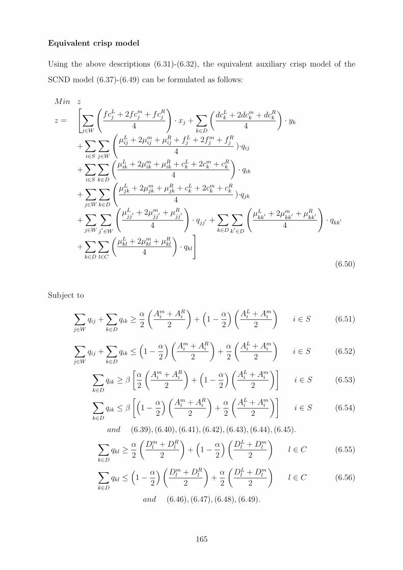
Equivalent crisp model
Using the above descriptions (6.31)-(6.32), the equivalent auxiliary crisp model of the
SCND model (6.37)-(6.49) can be formulated as follows:
Min z
z =
[
∑
j∈W
(
fcLj + 2fcmj + fcRj4
)
· xj +∑
k∈D
(
dcLk + 2dcmk + dcRk4
)
· yk
+∑
i∈S
∑
j∈W
(
µLij + 2µm
ij + µRij + fL
j + 2fmj + fR
j
4)·qij
+∑
i∈S
∑
k∈D
(
µLik + 2µm
ik + µRik + cLk + 2cmk + cRk4
)
· qik
+∑
j∈W
∑
k∈D
(
µLjk + 2µm
jk + µRjk + cLk + 2cmk + cRk4
)·qjk
+∑
j∈W
∑
j′∈W
(
µL
jj′ + 2µm
jj′ + µR
jj′
4
)
· qjj′ +∑
k∈D
∑
k′∈D
(
µL
kk′ + 2µm
kk′ + µR
kk′
4
)
· qkk′
+∑
k∈D
∑
l∈C
(
µLkl + 2µm
kl + µRkl
4
)
· qkl
]
(6.50)
Subject to
∑
j∈W
qij +∑
k∈D
qik ≥α
2
(
Ami + AR
i
2
)
+(
1−α
2
)
(
ALi + Am
i
2
)
i ∈ S (6.51)
∑
j∈W
qij +∑
k∈D
qik ≤(
1−α
2
)
(
Ami + AR
i
2
)
+α
2
(
ALi + Am
i
2
)
i ∈ S (6.52)
∑
k∈D
qik ≥ β
[
α
2
(
Ami + AR
i
2
)
+(
1−α
2
)
(
ALi + Am
i
2
)]
i ∈ S (6.53)
∑
k∈D
qik ≤ β
[
(
1−α
2
)
(
Ami + AR
i
2
)
+α
2
(
ALi + Am
i
2
)]
i ∈ S (6.54)
and (6.39), (6.40), (6.41), (6.42), (6.43), (6.44), (6.45).
∑
k∈D
qkl ≥α
2
(
Dml +DR
l
2
)
+(
1−α
2
)
(
DLl +Dm
l
2
)
l ∈ C (6.55)
∑
k∈D
qkl ≤(
1−α
2
)
(
Dml +DR
l
2
)
+α
2
(
DLl +Dm
l
2
)
l ∈ C (6.56)
and (6.46), (6.47), (6.48), (6.49).
165
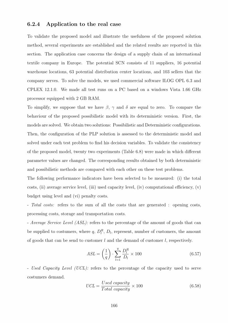
6.2.4 Application to the real case
To validate the proposed model and illustrate the usefulness of the proposed solution
method, several experiments are established and the related results are reported in this
section. The application case concerns the design of a supply chain of an international
textile company in Europe. The potential SCN consists of 11 suppliers, 16 potential
warehouse locations, 63 potential distribution center locations, and 103 sellers that the
company serves. To solve the models, we used commercial software ILOG OPL 6.3 and
CPLEX 12.1.0. We made all test runs on a PC based on a windows Vista 1.66 GHz
processor equipped with 2 GB RAM.
To simplify, we suppose that we have β, γ and δ are equal to zero. To compare the
behaviour of the proposed possibilistic model with its deterministic version. First, the
models are solved. We obtain two solutions: Possibilistic and Deterministic configurations.
Then, the configuration of the PLP solution is assessed to the deterministic model and
solved under each test problem to find his decision variables. To validate the consistency
of the proposed model, twenty two experiments (Table 6.8) were made in which different
parameter values are changed. The corresponding results obtained by both deterministic
and possibilistic methods are compared with each other on these test problems.
The following performance indicators have been selected to be measured: (i) the total
costs, (ii) average service level, (iii) used capacity level, (iv) computational efficiency, (v)
budget using level and (vi) penalty costs.
- Total costs: refers to the sum of all the costs that are generated : opening costs,
processing costs, storage and transportation costs.
- Average Service Level (ASL): refers to the percentage of the amount of goods that can
be supplied to costumers, where q, DRl , Dl, represent, number of customers, the amount
of goods that can be send to customer l and the demand of customer l, respectively.
ASL =
(
1
q
)
·
q∑
l=1
DRl
Dl
× 100 (6.57)
- Used Capacity Level (UCL): refers to the percentage of the capacity used to serve
costumers demand.
UCL =Used capacity
Total capacity× 100 (6.58)
166
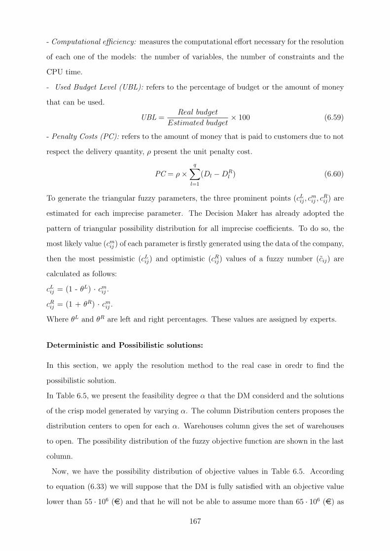
- Computational efficiency: measures the computational effort necessary for the resolution
of each one of the models: the number of variables, the number of constraints and the
CPU time.
- Used Budget Level (UBL): refers to the percentage of budget or the amount of money
that can be used.
UBL =Real budget
Estimated budget× 100 (6.59)
- Penalty Costs (PC): refers to the amount of money that is paid to customers due to not
respect the delivery quantity, ρ present the unit penalty cost.
PC = ρ×
q∑
l=1
(Dl −DRl ) (6.60)
To generate the triangular fuzzy parameters, the three prominent points (cLij, cmij , c
Rij) are
estimated for each imprecise parameter. The Decision Maker has already adopted the
pattern of triangular possibility distribution for all imprecise coefficients. To do so, the
most likely value (cmij ) of each parameter is firstly generated using the data of the company,
then the most pessimistic (cLij) and optimistic (cRij) values of a fuzzy number (cij) are
calculated as follows:
cLij = (1 - θL) · cmij .
cRij = (1 + θR) · cmij .
Where θL and θR are left and right percentages. These values are assigned by experts.
Deterministic and Possibilistic solutions:
In this section, we apply the resolution method to the real case in oredr to find the
possibilistic solution.
In Table 6.5, we present the feasibility degree α that the DM considerd and the solutions
of the crisp model generated by varying α. The column Distribution centers proposes the
distribution centers to open for each α. Warehouses column gives the set of warehouses
to open. The possibility distribution of the fuzzy objective function are shown in the last
column.
Now, we have the possibility distribution of objective values in Table 6.5. According
to equation (6.33) we will suppose that the DM is fully satisfied with an objective value
lower than 55 · 106 (e) and that he will not be able to assume more than 65 · 106 (e) as
167

Table 6.5: α-acceptable optimal solutions (part 1)
α Distribution centers Warehouses Possibility distribution of objective
zL(α) zm(α) zR(α)
0.1 CD7, CD22, CD24, CD49 F9 41 584 000 51 080 000 77 970 000
0.2 CD7, CD22, CD24, CD49 F9 42 180 000 51 825 000 79 088 000
0.3 CD7, CD22, CD24, CD49 F9 42 777 000 52 571 000 80 206 000
0.4 CD7, CD22, CD24, CD49 F9 43 373 000 53 316 000 81 324 000
0.5 CD7, CD22, CD24, CD49 F9 43 969 000 54 062 000 82 442 000
0.6 CD7, CD22, CD24, CD49 F9 44 566 000 54 807 000 83 560 000
0.7 CD7, CD22, CD24, CD49 F9 45 162 000 55 552 000 84 679 000
0.8 CD7, CD22, CD24 F9, F3 47 530 000 57 613 000 89 119 000
0.9 CD7, CD22, CD24 F9, F3 48 124 000 58 355 000 90 232 000
1 CD7, CD22, CD24 F9, F3 48 718 000 59 097 000 91 346 000
global cost. For simplicity we suppose that the membership function is linear, the goal
will be expressed as following:
µG(z) =
1 if z ≤ 55 · 106
65·106−z65·106−55·106
if 55 · 106 ≤ z ≤ 65 · 106
0 if z ≥ 65 · 106
(6.61)
We refer to equations (6.34) and (6.35) to calculate the compatibility index of each so-
lution with DM’s aspirations ( see equation (6.34)) and the membership degree of each
α-acceptable optimal solution (see equation (6.35)), as shown in Table 6.6. In agreement
with equation (6.36), the solution of the PLP model is the one which has the great-
est membership degree. We can see in Table 6.6 that the greatest membership degree
correspond to 0.32 and the 0.7-feasible optimal solution (Table 6.5) will be the best con-
figuration of the PLP problem.
In Table 6.7, we provide the number of variables, number of constraints, CPU Time, total
costs, distribution centers to open and warehouses to open for the deterministic model
and the probabilistic one. The capacity of each facility are presented between brackets.
Table 6.7 reveals that the deterministic model contains 12 671 variables and 18 765
constraints, and the computational time is equal to 912 seconds. The Possibilistic pro-
168

Table 6.6: α-acceptable optimal solutions (Part 2)
Feasibility degree α Satisfaction degree K α.K Optimal cost (e)
0.1 0.66 0.07 55 878 466
0.2 0.63 0.13 56 679 765
0.3 0.60 0.18 57 481 063
0.4 0.56 0.23 58 282 362
0.5 0.53 0.27 59 083 661
0.6 0.50 0.30 59 884 960
0.7 0.46 0.32 60 686 259
0.8 0.35 0.28 63 868 562
0.9 0.32 0.28 64 666 512
1 0.29 0.29 65 464 462
gramming model contains 12 671 variables and 18 868 constraints, the computational time
is 419 seconds. As we can see, the number of variables and constraints for the models
shows that they have the same degree of complexity. In addition, to satisfy customers
demand the warehouses and distribution centers to open are the same for the two models
with different capacities which are {F9} and {CD7, CD22, CD24, CD49} respectively.
Sensitivity analyses
To validate the consistency of the proposed model, twenty two experiments (Table 6.8)
were made in which different parameter values are changed. In the first experiments (1-
11), we analysed the effect of demand changes by changing the demand value and fixing
all other parameters. The next experiments (12-17) are set up to carry out the effect of
costs variations. Experiments (18-22) are designed to evaluate the variation of demand
and costs. Table 6.8 introduces details of the experiments.
The results of these experiments are given in (Table 6.9). We see that the possibilis-
tic model, in general, obtains better performance indicators (UCL, ASL, PC) and UBL)
than the deterministic model. Figure 6.6 presents the UBL values of each test problem.
As we can see, for deterministic model, 14 experiments have a budget using level more
than 100%, which represents 64% of cases. This means that the budget fixed using the
169

Table 6.7: Computational Results
Model Variables Constraints CPU Time (s) Total costs (e) Distribution centers Warehouses
Deterministic 12 671 18 765 912 55 493 965 CD7 (37 900 000) F9
CD22 (19 200 000)
CD24 (44 410 000)
CD49 (23 720 000)
Possibilistic 12 671 18 868 419 60 686 259 CD7 (39 740 000) F9
CD22 (19 600 000)
CD24 (45 410 000)
CD49 (24 250 000)
deterministic model (55 493 965 e) is not enough to satisfy the costumers in 64% of these
experiments. Whereas, only 5 test problems have exceeded the budget proposed by the
possibilistic model (60 686 259 e), therefore approximately 23% of test problems passed
the estimated budget. It is clear that the budget fixed by the PLP model is better than
the one proposed by the deterministic model, because with the first one, we succeed to
finance 77% of test cases and satisfy all customers, but with the second one, only 36%
of experiments are feasible to satisfy all customers. Although the possibilistic solution
is 9.3% more expensive than the deterministic one, this difference let us to get a robust
supply chain configuration that can absorb the uncertainty of environment, like price and
demand regulations, at the same time meet changing market requirements.
It can be seen from Table6.9 that the UBL average of deterministic configuration is equal
to 102%, so the majority of the UBL values are more than 100% (Figure 6.6), thus im-
plying that there is no sufficient money to take control of parameters uncertainties. The
UBL average of possibilistic solution (94%) reveals the flexibility and robustness of the
PLP solution in an uncertain environment.
Figure 6.7 shows the evolution of used capacity level varying the demand. As we can see,
increasing the demand the UCL of deterministic and possibilistic configurations rise until
to reach a peak (100%). The deterministic structure (125.23× 10⁶ pcs) attends capacity
peak before the possibilistic one (129 × 106 pcs). According to the results presented in
Table 6.9, the deterministic UCL average (96%) is bigger than the possibilistic one (94%).
170

Table 6.8: Experiments
N Experiment Description
1 The demands used in solving deterministic model
2 The demands are decreased by 3%
3 The demands are increased by 3%
4 The demands are increased by 5%
5 Demands The demands are decreased by 5%
6 The demands are increased by 10%
7 The demands are decreased by 10%
8 The demands are increased by 20%
9 The demands are decreased by 20%
10 The demands are increased by 30%
11 The demands are decreased by 30%
12 The costs are decreased by 10%
13 The costs are decreased by 5%
14 The costs are increased by 5%
15 Costs The costs are increased by 10%
16 The costs are increased by 15%
17 The costs are increased by 20%
18 The costs are increased by 2% and demands in-
creases by 2%
19 The costs are increased by 3% and demands in-
creases by 3%
20 Demands and
Costs
The cots are increased by 5% and demands are
decreased by 5%
21 The cots are increased by 10% and demands are
decreased by 8%
22 The cots are increased by 20% and demands are
decreased by 13%
171

Table 6.9: Possibilistic vs Deterministic Results
Exp Deterministic Possibilistic
UCL
(%)
ASL
(%)
PC (e) UBL (%) UCL
(%)
ASL
(%)
PC (e) UBL
(%)
1 100% 100% 0 100% 97% 100% 0 91%
2 97% 100% 0 98% 94% 100% 0 89%
3 100% 94% 748 200 102% 100% 100% 0 94%
4 100% 90% 1 252 200 104% 100% 98% 502 000 95%
5 95% 100% 0 96% 92% 100% 0 88%
6 100% 82% 2 508 200 108% 100% 94% 1 758 000 98%
7 90% 100% 0 92% 87% 100% 0 84%
8 100% 67% 5 006 200 115% 100% 86% 4 256 000 105%
9 80% 100% 0 85% 78% 100% 0 77%
10 100% 54% 7 509 412 123% 100% 79% 6 759 212 113%
11 70% 100% 0 77% 68% 100% 0 70%
12 100% 100% 0 90% 97% 100% 0 82%
13 100% 100% 0 95% 97% 100% 0 87%
14 100% 95% 1 233 199 105% 97% 100% 0 96%
15 100% 90% 2 466 398 110% 97% 99% 158 712 101%
16 100% 85% 3 699 597 115% 97% 94% 1 391 911 105%
17 100% 81% 4 728 260 119% 97% 90% 2 420 573 109%
18 100% 96% 500 540 104% 99% 100% 0 95%
19 100% 94% 750 856 105% 100% 100% 0 96%
20 95% 99% 239 348 101% 92% 100% 0 92%
21 92% 97% 800 508 103% 89% 100% 0 94%
22 87% 91% 1 979 624 108% 84% 100% 0 99%
Average96% 92% 1 453 126 102% 94% 97% 749 844 94%
172

90%
100%
110%
120%
130%
Budget�using�level(%)
60%
70%
80%
1 2 3 4 5 6 7 8 9 10 11 12 13 14 15 16 17 18 19 20 21 22 23
Experiments
Deterministic Possibilistic
Figure 6.6: Used budget level: Possibilistic vs Deterministic
70%
75%
80%
85%
90%
95%
100%
105%
Used�capacity�level�(%
)
60%
65%
70%
Demand
Deterministic Possibilistic
Figure 6.7: Used capacity level: Possibilistic vs Deterministic
173

70%
80%
90%
100%
110%
Average�service�level�(%
)
50%
60%
Demand
Deterministic Possibilistic
Figure 6.8: Average service level: Possibilistic vs Deterministic
As a result, this capacity abundance in possibilistic solution is necessary to control the
environment uncertainty, especially when the demand increases. Figure 6.8 exhibits the
average service level of deterministic and PLP models increasing the demand. We note
that for demand between 87.6 × 10⁶ to 129 × 106 pcs the possibilistic ASL is equal to
100%, when the demand attends maximal capacity of the structure (129×106) the service
level starts decreasing to attend approximately 80% when demand goes up to 162.7×10⁶.
For the deterministic configuration, ASL is between 94% and 100% growing the demand
from 87.6 × 10⁶ to 125.23 × 10⁶ pcs, then the level begins to go down (54%) increasing
demand from 125.23 × 10⁶ to 162.7 × 10⁶. These fluctuations are due to the insufficient
budget proposed by the deterministic model although, in these cases we have enough ca-
pacity. As seen in Table 6.9, the PLP models obtain ASL (97%) that are better than the
deterministic model (92%). In all cases, this possibilistic model is more better adapted
to the existing uncertainties in input parameters considered in this work.
Figure 6.9 resumes experiments where the company should pay penalties. The exper-
174

�������
�������
�������
�������
������
������
�������
�������
�����������������
�����
������������ �������������
�����
Figure 6.9: Penality: Possibilistic vs Deterministic
iments related to Possibilistic model show that when the demand increases from approxi-
mately 88× 106 to 129× 106, the penalty is equal to zero, exception one test problem the
penalty is equal to 2 420 573 (e) which is due to budget insufficiency to satisfy customers
demand. For demand values bigger than 129× 106, when the demand increases, then the
penalty costs increase significantly. On the other hand, the PC of deterministic model
fluctuates between zero and 4 728 260 (e) when the demand is increasing from approxi-
mately 88 × 106 to 129 × 106, then when the demand increases , the penalty value also
increases. In addition, we should pay penalty only five times in the possibilistic case,
which represents 34% of cases, but for the deterministic model we should do it in more
than 73% of cases, as can be seen in Figure 6.9.
6.2.5 Concluding Remarks
Determining the optimal supply chain configuration is a difficult problem since a lot of
factors and parameters must be taken into account when designing the network under
uncertainty. Since most of the parameters in such a problem have imprecise nature, a
175

PLP approach was used to model a supply chain network and, a possibilistic program-
ming resolution method was proposed, which is able to find an efficient solution based on
decision maker preferences.
The proposed model has been tested by using data from a real life textile SCN, hence
the results demonstrate the effectiveness of a Possibilistic Linear Programming approach
for SCND under uncertainty. In addition, this model controls the uncertainty sources
identified in SCN problems given lack of information such as demands, costs, process and
supply uncertainties.
The proposed possibilistic formulation is better than the deterministic methods for han-
dling the real situations where precise or certain future informations are not available
for SCND. Additionally, the possibilistic model supply chain performance indicators have
been seen to be clearly better than those of deterministic model, as previously shown. For
example, the average service level of PLP models (97%) are better than the determinis-
tic model (92%). The investment budget proposes by the first model is more important
than the second model, approximately 77% of the test cases are satisfied using the PLP
configuration and only 36% of them are feasible using the deterministic solution. Further-
more, the possibilistic model has not generated an excessive increment of computational
efficiency, then the possibility to model and solve a real life size supply chain problems
under uncertainty.
In the next Chapter, we will present the general conclusions of this thesis.
176

Chapter 7
Conclusions and Perspectives
The work presented in this thesis is a relative small contribution in the Supply Chain
research ocean. However, we think that design multi-criteria Supply Chain under uncer-
tainty is really a contemporary issue in many application domains.
Chapter 2 presented a review of mathematical programming models and resolution meth-
ods for Supply Chain Network Design (SCND). We have proposed a classification based
on the analysis of three aspects: supply chain network structure, decision level, supply
chain modeling approach. The conclusions drawn from this chapter affirm that: (i) papers
integrating multiple periods, multiple products, multiple criteria, multiple transportation
modes, multiple objective and uncertainty in SCND context are still scarce, (ii) the most
widely used modeling approach is mixed integer linear programming, where the use of
heuristic algorithms and meta-heuristics to solve the approach stands out, (iii) more pro-
posed models are validated using small numerical examples and the number of case studies
applied to real supply chains are still scare.
Chapter 3 studied our new multi-criteria supply chain network design methodology.
We have integrated many aspects in the design of the optimal sustainable supply chain,
such as: economical, social, environmental and legislative aspects.
Our methodology consists of two different steps. In the first step, we find the best poten-
tial facility locations where the future facilities could be established and different criteria
are satisfied. To model this step, we have combined the Geographic Information System
(GIS) and the AHP method. The second step establishes the optimal supply chain design
177

to achieve customer demands and economic criteria using Mixed Integer Linear Program-
ming model.
A computational real case study has demonstrated the methodology’s efficiency, and has
shown that using GIS model to locate potential facilities in the design of sustainable sup-
ply chain network is very useful. In fact, it has provided a good way for integrating many
criteria and constraints such as: location sites far from the urban areas; sites should be
close to commercial zones, roads, railways and landfills; plants should be far from natural
area, airports and agriculture area, etc. Also, the GIS model has reduced the potential
set of locations from the entire country or region to small sustainable locations set. This
speeds up the process of finding the optimal supply chain configuration in the next step.
Our second contribution in this chapter is the study of CO2 emission impacts in the SCND.
We have shown that the integration of the environmental costs and multi-modality in the
mathematical model changes the structure of the supply chain network. It depends on
the environmental policy of the Company. This means that using the model, supply chain
managers could be able to see the impact of integration of the CO2 taxes and multi-modal
transportation network in the strategic decisions of supply chain. That will help them
to select the best strategic supply chain network. From this chapter we have learned
that integration of environmental taxes in the model can be an efficient way to achieve
environmental goals, by choosing the best SCN and clean transportation modes. These
results have also confirmed that to reduce CO2 emissions, we should take into account
multi-modal transport network, in the design of the supply chain.
Therefore, many possible future research avenues can be defined in this context. For in-
stance, GIS has the potential to speed up the process of finding potential locations and to
permit sensitivity analysis that will examine the impact of varying some of the criteria in
a mapping exercise. The results of this analysis can be used to identify general areas to
be further evaluated on a site specific basis using more detailed market place information.
As job opportunities or population features change due to actual development, the model
can be easily revised to reflect these changes. In addition, the second step model should
have objectives to evaluate the impact quality, lead-time and service level in supply chain
design problem. Also, we think that it is very important to compare the results of our
methodology to the existent SCND framework.
178
Chapter 4 presented an extension of the second step of the methodology proposed in
Chapter 3. We have proposed a multi-objective supply chain network design problem.
We have formulated the problem as a Goal Programming model which aims at achieving
four economics and environmental goals which are respectively: (i) total costs goal, (ii)
energy consumption costs goal, (iii) waste treatment costs goal and (iv) CO2 emissions
goal. We have conducted a sensitivity analysis for the case study and we have observed
that, improving the building technology and increasing the facility number in the supply
chain can decrease CO2 emission of the whole network. Also, the total cost increase is
expected to be in conflict with the other three goals that aim to reduce the CO2 emission,
energy consumption and waste treatment of the supply chain. Regarding to the influence
of some parameters on the SC configuration and transportation mode used, we have found
that small variability of goals weight ωi does not affect the solution.
Our further research direction is to consider more factors in supply chain, such as social
criteria, quality criteria and taking into account the product life cycle. On the other
hand, we can also extend our research through designing new solution methods to solve
this multi-objective supply chain network design model, such as heuristics and meta-
heuristics.
Chapter 5 proposed a three-phase heuristic decomposition algorithm to solve large-
scale supply chain network design problems. The heuristic consists of three phases which
are: (i) decomposition phase, (ii) reduction phase and (iii) resolution phase. In the de-
composition phase, we divide the large scale supply chain network into small two-layer
networks. In reduction phase, we use a modified p-median model to reduce the large
potential sets into small reduced sets. In resolution phase, we use a global MILP model
to solve the reduced supply chain network.
Very large problems can indeed be solved in a reasonable amount of time with the heuristic,
whereas they cannot be solved with conventional MIP tools within a reasonable amount
of computational time. We have solved a real large-scale supply chain network composed
of 220 suppliers, 220 warehouses, 220 distribution centers and 1 500 customers, in less
than 550 seconds. The numerical experiments have indicated that the proposed heuris-
179

tic solution algorithm performs well in terms of solution quality and computational time
consumed. For example, the average of heuristic CPU Time is equal to 5 seconds for
small size instances, 24 seconds for medium size problems and only 115 seconds for large
scale instances. Moreover, the gap between the final solution obtained by the proposed
heuristic approach and the lower bound of global MILP obtained by Cplex is equal to
0% in small size instances, less than 0.52% in medium size instances and in large size
problems, the gap ranges from 1.19% to 9.52% and the average gap between the lower
bound of the global MILP model and the solution of the heuristic is equal to 5.66%.
Future research could consider systems that faced not only deterministic parameters but
also stochastic parameters. The proposed solution approach can be adapted to other
SCN problems such as reverse logistic network design problem. In addition, it would
be interesting to apply this algorithm to more complex supply chains with more stages
and considering the SC parameters uncertainty. Furthermore it is possible to compare
the performance of this heuristic to others resolution methods presented in the literature.
Another unexplored extension of this algorithm is the consideration of a more complex
SCND model with multiple products, multiple periods, multiple objectives and uncertain
SC parameters.
Chapter 6 presented a supply chain design problem which includes explicitly demand
uncertainty. We use two-stage stochastic programming formulation to model the problem.
The results obtained pointed out, that supply chain design methods which do not include
uncertainty obtain inferior results if compared with models that formalise it implicitly.
The stochastic model could handle data uncertainty with a reasonable increase in total
costs compared with the deterministic model and therefore it can be concluded that the
proposed two-stage programming model can be used as a robust model in real cases.
Many possible future research directions can be defined in the area of logistic network
design under uncertainty. For example addressing uncertainty for all variable costs and
potential locations of customers may be attractive direction for future research. Moreover,
time complexity is not addressed in this chapter. However, since the computational time
increases when the size of the problem and the number of scenarios increase. We also need
to reduce the runtime further in order to include more scenarios and add more facilities
180

to the supply chain design decisions. Therefore, developing efficient exact or heuristic
solution methods is also a critical need in this area.
Since most of the parameters in our problem have imprecise nature and the complexity
to solve it by using the two-stage stochastic programming, we have proposed Possibilistic
Linear Programming (PLP) approach to model a supply chain network and which is able
to find an efficient solution based on decision maker preferences in a reasonable time.
The proposed model in this Chapter has been tested by using data from a real life textile
SCN, hence the results have demonstrated the effectiveness of a Possibilistic Linear Pro-
gramming approach for SCND under uncertainty. In addition, this model has controlled
the uncertainty sources identified in SCN problems given lack of information such as de-
mands, costs, process and supply uncertainties.
The proposed possibilistic formulation is better than the deterministic methods for han-
dling the real situations where precise or certain future informations are not available
for SCND. Additionally, the possibilistic model supply chain performance indicators have
been seen to be clearly better than those of deterministic model, as previously shown.
Furthermore, the possibilistic model has not generated an excessive increment of com-
putational efficiency, then the possibility to model and solve a real life size supply chain
problems with more uncertain parameters.
An interesting future research topic is to integrate into the proposed supply chain model
other aspects, such as multi-period, multi-product and multi-objective. In addition, the
CPU time was not an issue in our numerical experiments. However, in other large scaled
practical problems it might be an issue. Therefore, developing an efficient heuristic or
meta-heuristic algorithm to solve the corresponding PLP models should be helpful in
reaching efficient solutions in reasonable time.
This concludes our thesis. Our hope is that it will at least stimulate discussion among
researcher working in Supply Chain Network Design , about the usefulness of considering
Multi-criteria aspect and data uncertainty mixed approaches.
181

Appendix A
Figures and Tables
A.1 AHP Example
We start by presenting the AHP example, then we explain how to elaborate the pairwise
comparison matrix and how to calculate the importance ratios.
A company wishes to buy a new production equipment and has defined many aspects
to chose the machine. We assume a firm has three criteria: cost, quality and delivery-
time. The high level in the hierarchy graph concerns the effective selection of the best
equipment; the following level represents criteria that correspond to the firm objectives;
and the last level with the selection of the alternative suppliers.
What weights should you put on each of these equipments? Is the A, B or C the ultimate
machine? Can you ignore any of these criteria ? It’s time for the AHP.
We first provide a matrix for the company’s pairwise comparisons using the evaluation
scale to make pairwise comparisons between criteria importance according to objective
achievement. Let us say that we compared all these criteria and come up with this table
(Table A.1). Table.A.1 is read as follows:
- 1, indicates the equal importance of the criteria.
- 5, indicates that cost is considerably more important than quality.
- 9, indicates that cost is strongly more important than delivery-time.
- 3, indicate that the quality is moderately important than delivery-time.
A little matrix now lets us to turn these comparisons into numerical weight. First, we
want to normalize all weights to a common references, by adding up the weights in a
182

Table A.1: Comparison between criteria
Preference signification Cost Quality Delivery-time
Cost 1 5 9
Quality 0.2 1 3
Delivery-time 0.11 0.33 1
Total 1.61 6.33 13
column; then we divide each weight by its column sum. For example, as we can see on
Table A.1, the sum of the weights in the Delivery time column is 13. Then we divide
each weight in Delivery time column by 13 so the weight for cost is 9/13 or 0.69. This
normalizes all weights to a common references. The next step is to calculate the average
Table A.2: Relative importance ratios
Preference signification Cost Quality Delivery-time Raw average
Cost 0.76 0.79 0.69 0.75
Quality 0.15 0.16 0.23 0.18
Delivery-time 0.08 0.05 0.08 0.07
Total 1 1 1 1
of the normalized weights of each criteria to obtain the raw average column in Table A.2.
For example, the weight of the quality criteria is equal to 0.18 (Table A.2).
The AHP has revealed that for this company the cost is the most important criteria.
Without AHP, may we have assumed hat the ultimate criteria was Quality or Delivery
time.
A.2 Figures and Tables
183

Figure A.1: Sediments depots in NPDC region
Légende
Réseau Routier
0 - 624
624 - 1 249
1 249- 1 874
1 874- 2 499
2 499 - 3 124
3 124 - 3 749
3 749 - 4 374
4 374 - 4 999
4 999 - 5 623
5 623 - 6 248
.
0 20 40 60 8010
Kilomètres BOUZEMBRAK Y., MASSON E. 2010
Figure A.2: Roads network classes in NPDC region
Table A.3: Roads network classes and weights
Classes Weights Classes Weights
0 – 624 9 3 124 - 3 749 5
624 – 1 249 9 3 749 - 4 374 4
1 249 - 1 874 8 4 374 - 4 999 3
1 874 - 2 499 7 4 999 - 5 623 2
2 499 - 3 124 6 5 623 - 6 248 1
184
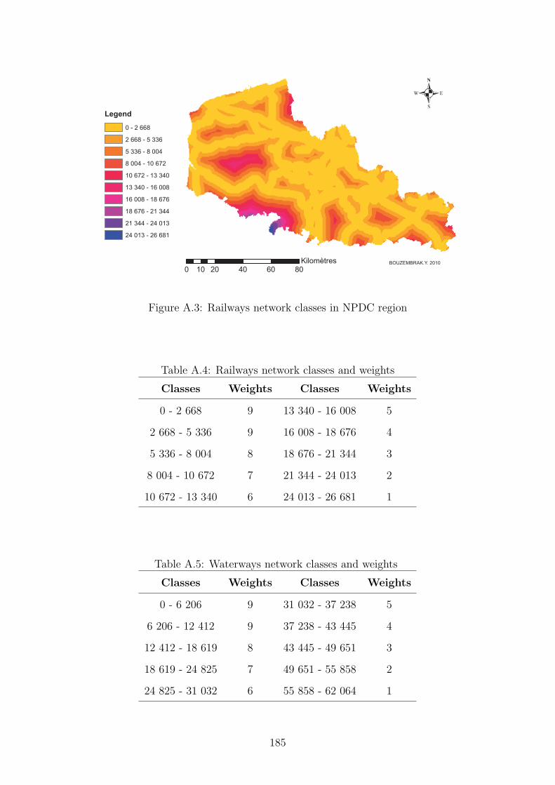
Legend
0 - 2 668
2 668 - 5 336
5 336 - 8 004
8 004 - 10 672
10 672 - 13 340
13 340 - 16 008
16 008 - 18 676
18 676 - 21 344
21 344 - 24 013
24 013 - 26 681
.
0 20 40 60 8010
Kilomètres BOUZEMBRAK.Y. 2010
Figure A.3: Railways network classes in NPDC region
Table A.4: Railways network classes and weights
Classes Weights Classes Weights
0 - 2 668 9 13 340 - 16 008 5
2 668 - 5 336 9 16 008 - 18 676 4
5 336 - 8 004 8 18 676 - 21 344 3
8 004 - 10 672 7 21 344 - 24 013 2
10 672 - 13 340 6 24 013 - 26 681 1
Table A.5: Waterways network classes and weights
Classes Weights Classes Weights
0 - 6 206 9 31 032 - 37 238 5
6 206 - 12 412 9 37 238 - 43 445 4
12 412 - 18 619 8 43 445 - 49 651 3
18 619 - 24 825 7 49 651 - 55 858 2
24 825 - 31 032 6 55 858 - 62 064 1
185

Figure A.4: Waterways network classes in NPDC region
Legend
0 - 6 379
6 379 - 12 759
12 759 - 19 138
19 138 - 25 518
25 518 - 31 897
31 897 - 38 277
38 277 - 44 656
44 656 - 51 036
51 036 - 57 415
57 415 - 63 795
.
0 10 20 30 405
Kilomètres BOUZEMBRAK.Y. 2010
Figure A.5: VNF landfills classes
186

Table A.6: Landfills classes and weights
Classes Weights Classes Weights
0 - 6 379 9 31 897 - 38 277 5
6 379 - 12 759 9 38 277 - 44 656 4
12 759 - 19 138 8 44 656 - 51 036 3
19 138 - 25 518 7 51 036 - 57 415 2
25 518 - 31 897 6 57 415 - 63 795 1
Legend
0 - 5 839
5 839 - 11 679
11 679 - 17 518
17 518 - 23 358
23 358 - 29 197
29 197 - 35 037
35 037 - 40 877
40 877 - 46 716
46 716 - 52 556
52 556 - 58 395
.
0 20 40 60 8010
Kilomètres BOUZEMBRAK.Y. 2010
Figure A.6: Brownfield classes in NPDC region
Table A.7: Brownfield classes and weights
Classes Weights Classes Weights
0 - 5 839 9 29 197 - 35 037 5
5 839 – 11 679 9 35 037 - 40 877 4
11 679 – 17 518 8 40 877 - 46 716 3
17 518 - 23 358 7 46 716 - 52 556 2
23 358 - 29 197 6 52 556 - 58 395 1
187
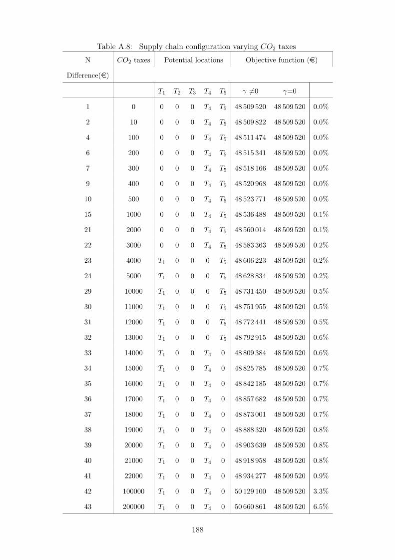
Table A.8: Supply chain configuration varying CO2 taxes
N CO2 taxes Potential locations Objective function (e)
Difference(e)
T1 T2 T3 T4 T5 γ 6=0 γ=0
1 0 0 0 0 T4 T5 48 509 520 48 509 520 0.0%
2 10 0 0 0 T4 T5 48 509 822 48 509 520 0.0%
4 100 0 0 0 T4 T5 48 511 474 48 509 520 0.0%
6 200 0 0 0 T4 T5 48 515 341 48 509 520 0.0%
7 300 0 0 0 T4 T5 48 518 166 48 509 520 0.0%
9 400 0 0 0 T4 T5 48 520 968 48 509 520 0.0%
10 500 0 0 0 T4 T5 48 523 771 48 509 520 0.0%
15 1000 0 0 0 T4 T5 48 536 488 48 509 520 0.1%
21 2000 0 0 0 T4 T5 48 560 014 48 509 520 0.1%
22 3000 0 0 0 T4 T5 48 583 363 48 509 520 0.2%
23 4000 T1 0 0 0 T5 48 606 223 48 509 520 0.2%
24 5000 T1 0 0 0 T5 48 628 834 48 509 520 0.2%
29 10000 T1 0 0 0 T5 48 731 450 48 509 520 0.5%
30 11000 T1 0 0 0 T5 48 751 955 48 509 520 0.5%
31 12000 T1 0 0 0 T5 48 772 441 48 509 520 0.5%
32 13000 T1 0 0 0 T5 48 792 915 48 509 520 0.6%
33 14000 T1 0 0 T4 0 48 809 384 48 509 520 0.6%
34 15000 T1 0 0 T4 0 48 825 785 48 509 520 0.7%
35 16000 T1 0 0 T4 0 48 842 185 48 509 520 0.7%
36 17000 T1 0 0 T4 0 48 857 682 48 509 520 0.7%
37 18000 T1 0 0 T4 0 48 873 001 48 509 520 0.7%
38 19000 T1 0 0 T4 0 48 888 320 48 509 520 0.8%
39 20000 T1 0 0 T4 0 48 903 639 48 509 520 0.8%
40 21000 T1 0 0 T4 0 48 918 958 48 509 520 0.8%
41 22000 T1 0 0 T4 0 48 934 277 48 509 520 0.9%
42 100000 T1 0 0 T4 0 50 129 100 48 509 520 3.3%
43 200000 T1 0 0 T4 0 50 660 861 48 509 520 6.5%
188

Table A.9: CO2 Emissions varying CO2 taxes
N CO2 taxes Potential locations CO2 Emissions (T)
T1 T2 T3 T4 T5 γ 6=0 γ=0 Difference (%)
1 0 0 0 0 T4 T5 980 980 0.0%
2 10 0 0 0 T4 T5 302 980 69.2%
4 100 0 0 0 T4 T5 290 980 70.4%
6 200 0 0 0 T4 T5 286 980 70.8%
7 300 0 0 0 T4 T5 280 980 71.4%
9 400 0 0 0 T4 T5 280 980 71.4%
10 500 0 0 0 T4 T5 280 980 71.4%
15 1000 0 0 0 T4 T5 240 980 75.5%
21 2000 0 0 0 T4 T5 235 980 76.0%
22 3000 0 0 0 T4 T5 233 980 76.2%
23 4000 T1 0 0 0 T5 226 980 76.9%
24 5000 T1 0 0 0 T5 205 980 79.0%
29 10000 T1 0 0 0 T5 205 980 79.1%
30 11000 T1 0 0 0 T5 205 980 79.1%
31 12000 T1 0 0 0 T5 205 980 79.1%
32 13000 T1 0 0 0 T5 205 980 79.1%
33 14000 T1 0 0 T4 0 164 980 83.3%
34 15000 T1 0 0 T4 0 164 980 83.3%
35 16000 T1 0 0 T4 0 164 980 83.3%
36 17000 T1 0 0 T4 0 153 980 84.4%
37 18000 T1 0 0 T4 0 153 980 84.4%
38 19000 T1 0 0 T4 0 153 980 84.4%
39 20000 T1 0 0 T4 0 153 980 84.4%
40 21000 T1 0 0 T4 0 153 980 84.4%
41 22000 T1 0 0 T4 0 153 980 84.4%
42 100000 T1 0 0 T4 0 153 980 84.4%
43 200000 T1 0 0 T4 0 153 980 84.4%
189

Table A.10: Transportation modes used varying CO2 taxes
N CO2 taxes Potential locations Transportation Modes Optimal Solution (e)
T1 T2 T3 T4 T5 % Roads % Waters % Trains
1 0 0 0 0 T4 T5 9.3% 80.7% 10% 48 509 520
2 10 0 0 0 T4 T5 0.0% 78% 22% 48 509 822
4 100 0 0 0 T4 T5 0% 75.3% 24.7% 48 511 474
6 200 0 0 0 T4 T5 0% 74.7% 25.3% 48 515 341
7 300 0 0 0 T4 T5 0% 54.7% 45.3% 48 519 567
9 400 0 0 0 T4 T5 0% 54.7% 45.3% 48 523 771
10 500 0 0 0 T4 T5 0% 54.7% 45.3% 48 526 526
15 1000 0 0 0 T4 T5 0% 53.3% 46.7% 48 538 824
21 2000 0 0 0 T4 T5 0% 52.0% 48.0% 48 583 363
22 3000 0 0 0 T4 T5 0% 36.7% 63.3% 48 606 223
23 4000 T1 0 0 0 T5 0.7% 36.7% 62.7% 48 628 834
24 5000 T1 0 0 0 T5 0.7% 36.7% 62.7% 48 649 368
29 10000 T1 0 0 0 T5 0.7% 36.7% 62.7% 48 751 955
30 11000 T1 0 0 0 T5 0.7% 36.7% 62.7% 48 772 441
31 12000 T1 0 0 0 T5 0.7% 36.7% 62.7% 48 792 915
32 13000 T1 0 0 0 T5 1.3% 25.3% 73.3% 48 809 384
33 14000 T1 0 0 T4 0 1.3% 25.3% 73.3% 48 825 785
34 15000 T1 0 0 T4 0 1.3% 25.3% 73.3% 48 842 185
35 16000 T1 0 0 T4 0 2.0% 25.3% 72.7% 48 857 682
36 17000 T1 0 0 T4 0 2.0% 25.3% 72.7% 48 873 001
37 18000 T1 0 0 T4 0 2.0% 25.3% 72.7% 48 888 320
38 19000 T1 0 0 T4 0 2.0% 25.3% 72.7% 48 903 639
39 20000 T1 0 0 T4 0 2.0% 25.3% 72.7% 48 918 958
40 21000 T1 0 0 T4 0 2.0% 25.3% 72.7% 48 934 277
41 22000 T1 0 0 T4 0 2.0% 24.7% 73.3% 50 129 100
42 100000 T1 0 0 T4 0 2.0% 24.7% 73.3% 51 660 861
43 200000 T1 0 0 T4 0 50 660 861 48 563 113 48 509 520 0%
190

Figure A.7: GIS Model
191

Table A.11: Law demand case
Treatment facility
Scenarios Optimal solution cost (e) T1 T2 T3 T4 T5
S1 21 499 647 0 0 0 0 1
S2 22 371 138 1 0 0 0 0
S3 22 663 786 0 0 0 0 1
S4 23 190 979 0 0 0 0 1
S5 22 734 047 0 0 0 0 1
S6 22 557 098 1 0 0 0 0
S7 22 136 323 0 0 0 0 1
S8 22 915 831 0 0 0 0 1
S9 22 373 920 1 0 0 0 0
S10 22 880 011 0 0 0 0 1
S11 22 663 442 1 0 0 0 0
S12 21 497 861 0 0 0 0 1
S13 21 845 157 0 0 0 0 1
S14 22 014 339 1 0 0 0 0
S15 22 841 817 0 0 0 0 1
S16 22 416 860 0 0 0 0 1
S17 21 890 644 0 0 0 0 1
S18 22 862 889 0 0 0 0 1
S19 22 840 508 0 0 0 0 1
S20 22 511 297 0 0 0 0 1
S21 22 685 309 1 0 0 0 0
S22 22 011 263 0 0 0 0 1
S23 21 669 811 0 0 0 0 1
S24 22 607 973 1 0 0 0 0
192

Table A.12: Medium demand case
treatment facilities
Scenarios Objective Value (e) T1 T2 T3 T4 T5
S25 51 537 458 0 0 0 1 1
S26 47 741 375 1 0 0 0 1
S27 48 164 175 0 0 0 1 1
S28 49 404 226 0 0 0 1 1
S29 51 771 159 1 0 0 0 1
S30 47 241 512 0 0 0 1 1
S31 48 872 672 1 0 0 0 1
S32 51 381 933 1 0 0 0 1
S33 48 471 592 1 0 0 0 1
S34 46 914 566 0 0 0 1 1
S35 49 214 544 0 0 0 1 1
S36 46 952 201 1 0 0 0 1
S37 47 050 298 0 0 0 1 1
S38 49 170 072 0 0 0 1 1
S40 48 368 435 1 0 0 0 1
S41 47 266 430 1 0 0 0 1
S42 46 956 496 0 0 0 1 1
S43 49 962 501 1 0 0 0 1
S44 67 772 882 1 0 0 1 1
S45 47 581 870 0 0 0 1 1
S46 46 315 504 0 0 0 1 1
S47 48 817 042 0 0 0 1 1
S48 46 963 658 0 0 0 1 1
S49 67 421 795 1 0 0 1 1
193

Table A.13: High demand case
Treatment facility
Scenarios Objective Value (e) T1 T2 T3 T4 T5
S50 74 846 906 1 0 0 1 1
S51 76 158 613 1 0 0 1 1
S52 76 181 000 1 0 0 1 1
S53 74 754 634 1 0 0 1 1
S54 74 195 625 1 0 0 1 1
S55 77 318 660 1 0 0 1 1
S56 71 685 345 1 0 0 1 1
S57 76 215 353 1 0 0 1 1
S58 74 372 451 1 0 0 1 1
S59 76 026 390 1 0 0 1 1
S60 76 804 009 1 0 0 1 1
S61 72 449 642 1 0 0 1 1
S62 75 644 260 1 0 0 1 1
S63 73 683 304 1 0 0 1 1
S64 74 667 875 1 0 0 1 1
S65 76 076 986 1 0 0 1 1
S66 75 289 961 1 0 0 1 1
S68 73 296 110 1 0 0 1 1
S69 73 296 110 1 0 0 1 1
S70 73 335 197 1 0 0 1 1
S71 76 956 521 1 0 0 1 1
S72 75 403 173 1 0 0 1 1
S73 76 787 453 1 0 0 1 1
S74 75 981 418 1 0 0 1 1
194

195

195��
Bibliography Aghezzaf, E. (2005). Capacity planning and warehouse location in supply chains with uncertain demands, Journal of the Operational Research Society, 56, 453–462.
Ahmed, S., Sahinidis, N.V. ( 2003). An approximation scheme for stochastic integer programs arising in capacity expansion. Operations Research, 51, 461-471.
Akyol, D.E. , Bayhan, G. M. (2007). A review on evolution of production scheduling with neural networks, Computers & Industrial Engineering, 53, 95–122.
Alçada-Almeida, L., Coutinho-Rodrigues, J., Current, J. (2009). A multiobjective modeling approach to locating incinerators, Socio-Economic Planning Sciences, 43, 111–120.
Aliev, R.A., Fazlollahi, B., Guirimov, B.G., Aliev, R.R. (2007). Fuzzy-genetic approach to aggregate production–distribution planning in supply chain management. Information Sciences, 177, 4241–4255.
Alonso-Ayuso, A., Escudero, L.F., Garin, A., Ortuno, M.T., Perez, G. (2003). An approach for strategic supply chain planning under uncertainty based on stochastic 0–1 programming. Journal of Global Optimization, 26, 97-124.
Altiparmak, F., Gen, M., Lin, L., Paksoy, T. (2006). A genetic algorithm approach for multiobjective optimization of supply chain networks. Computers and Industrial Engineering, 51, 196–215.
Ambrosino, D., Scutellà, M.G. (2005). Distribution network design: New problems and related models, European Journal of Operational Research, 165, 610– 624.
Amiri, A. (2006). Designing a distribution network in a supply chain system: Formulation and efficient solution procedure. European Journal of Operational Research , 171, 567-576.
Amrani, H., Martel, A., Zuerey, N., Makeeva, P. (2008). A Variable Neighborhood Search Heuristic for the Designof Multicommodity Production-Distribution Networks with Alternative Facility Congurations. CIRRELT Research Document,Universit Laval, Canada , 35.
Amtzen, B.C., Brown, G.G., Harrison, T.P., Trafton, L.L. (1995), Global supply chain management at Digital Equipment Corporation, Interfaces, 25 (1), 69-93.
Andersson, H., Hoff, A., Christiansen, M., Hasle, G., Lokketangen, A. (2010) . Industrial aspects and literature survey: Combined inventory management and routing, Computers & Operations Research 37, 1515–1536.
Aouni, B., Kettani, O. (2001). Goal Programming model: A glorious history and a promesing future. International Journal of Operational Research, 133, 225-231.
Aras, H., Erdurmuse, S., Koc, E., (2002) . Multi-criteria selection for a restauration location in Taipei, Hospital Management, 21, 171–187.
Arcview.9.3. (2010). Arcview Manual. http://www.esrifrance.fr/ArcView.asp
Arntzen, B., Brown, G., Harrison, T., Trafton, L. (1995). Global supply chain management at digital equipment corporation. Interfaces , 21 (1), 69-93.

196��
Azaron, A., Borwn, K.N., Tarim, S.A., Modarres, M. (2008). A multi-objective stochastic programming approach for supply chain design considering risk. International Journal of Production Economics, 116, 129–138.
Banks, E. (2006). Catastrophic risk: Analysis and Management. Wiley Finance.
Barahona, F., Chudak, F.A. (2005). Near-optimal Solutions to Large-scale Facility Location Problems. Discrete Optimization 2, 35-50.
Barbosa-Povoa. (2009). Sustainable supply chains . Computer aided chemical engineering. Elsevier: Brazil, 127-132
Barda, O.H. , Dupuis, J., Lencioni, P. (1990). Multicriteria location of thermal power plants, European Journal of Operational Research, 45, 332–346.
Barros, A.I., Dekker, R., Scholten, V. (1998). A two-level network for recycling sand: A case study, European Journal of Operational Research, 110, 199–214.
Bellman, R.E., Zadeh, L. (1970) . Decision making in a fuzzy environment, Management Science. 17, 141–164.
Benders, J. F. (1962). Partitioning procedures for solving mixed-variable programming problems, Numerische Mathematik, 4, 238–252
Ben-Haim, Y., Elishakoff, I. (1990). Convex Models of Uncertainty in Applied Mechanics, Elsevier, Amsterdam.
Berry, D., Towill, DR., Wadsley, N. (1994). Supply chain management in the electronics products industry. International Journal of Physical Distri-bution and Logistics Management, 24(10), 20–32.
Birge J.R., Louveaux , F. (1997). Introduction to Stochastic Programming, Springer.
Bloemhof-Ruwaard, J.M., Salomon, M., Van Wassenhove, L.N. (1994), On the coordination of product and byproduct flows in two-level distribution networks: Model formulations and solution procedures, European Journal of Operational Research,79, 325-339.
Bojarski, A.D., Lainez, J.M., Espuna, A., Puigjaner, L. (2009). Incorporating environmental impacts and regulations in a holistic supply chains modeling: An LCA approach. Computers Chemical Engineering, 33(10), 1747-1759.
Bok, J., Lee, H., Park, S. (1998). Robust investment model for long-range capacity expansion of chemical processing networks under uncertain demand forecast scenarios. Computers and Chemical Engineering, 22, 7, 1037-1049.
Bouzembrak, Y., Allaoui, H., Goncalves, G., Masson, E., Bouchriha, H., Baklouti, M. (2010). Sustainable Multimodal Supply Chain Design for recycling waterways sediments. 8th International Conference of Modeling and Simulation - MOSIM10, May 10-12, Hammamet, Tunisia.
Bowersox, D.J., Closs, D.J., Cooper, M.B. (2002). Supply Chain Logistics Management. McGrawHill Irwin, Boston, MA.
Brown, G.G., Olson, M.P. (1994), Dynamic factorization in large-scale optimization, Mathematical Programming , 64, 17- 51.
197��
Brown, G.G., Graves, G.W., Honczarenko, M.D. (1987). Design and operation of a multicommodity production/ distribution system using primal goal decomposition. Management Science, 33 (11), 1469–1480.
Buckley, J.J. (1988). Possibilistic programming with triangular fuzzy numbers. Fuzzy Sets and Systems, 26, 135–138.
Buckley, J.J. (1989). Solving possibilistic linear programming problems. Fuzzy Sets and Systems, 31, 329–341.
Canel, C., Khumawala, B.M., Law, J., Loh, A. (2001). An algorithm for the capacitated, multi-commodity multi-period facility location problem, Computers & Operations Research, 28, 411–427.
Canel, C., Khumawala, B.M. (1997) . Multi-period international facilities location: An algorithm and application, International Journal of Production Economics, 35, 1891–1910.
Cantarella, G.E., Vitetta, A. (2006). The multi-criteria road network design problem in an urban area, Transportation, 33, 567–588.
Canbolat, Y.B., Chelst, K., Garg, N. (2007). Combining decision tree and MAUT for selecting a country for a global manufacturing facility, Omega, 35, 312– 325.
Carlsson, D., Rönnqvist, M. (2005) . Supply chain management in forestry – Case studies at södra cell AB, European Journal of Operational Research, 163, 589–616.
Charnes, A., Cooper, W.W. (1961). Management Models and Industrial Applications of linear Programming, Wiley, New York.
Charnes, A., Cooper, W.W., Ferguson, R. (1955). Optimal estimation of executive compensation by linear programming Management Science, 1 , 138-151.
Chen, C.L , Lee, W.C. (2004) . Multi-objective optimization of multi-echelon supply chain networks with uncertain product demands and prices, Computers and Chemical Engineering, 28, 1131–1144.
Cheng, C. B., Wang, K. P. (2009). Solving a vehicle routing problem with time windows by a decomposition technique and a genetic algorithm. Expert Systems with Applications, 36(4), 7758-7763.
Chopra, S., Meindl, P. (2004) . Supply Chain Management: Strategy, Planning and Operation. Prentice Hall, Upper Saddle River, USA.
Christopher, M., Lee, H. (2004). Mitigating supply chain risk through improved confidence. International Journal of Physical Distribution & Logistics Management, 34, 5, 388-396.
Christopher, M. (2001). Logistics and supply chain management: creating value-added networks. Second edition, Great Britin.
Cohen, M.A., Fisher, M., Jaiknamar, R. (1989). International manufacturing and distribution networks: A normative model framework, in: K. Ferdows, ed, Managing International Manufacturing, North-Holland, Amsterdam, 67-93.
Cohen, M.A., Kleindorfer, P.R. (1993). Creating value through operations: The legacy of Elwood S. Buffa, in: R.K. Satin, ed., Perspectives in Operations" Management (Essays in Honor of Elwood S. Buffh), Kluwer Academic Publishers, Boston, MA, 3-21.

198��
Cohen, M.A., Lee, H.L. (1985). Manufacturing strategy: Concepts and methods, Chapter 5.In: Kleindorfer, P.R. (Ed.), The Management of Productivity and Technology in Manufacturing. Plenum Press, New York, 153– 188.
Cohen, M.A., Lee, H.L. (1989). Resource deployment analysis of global manufacturing and distribution networks.Journal of Manufacturing Operations Management, 2, 81–104.
Cohen, M.A., Moon, S. (1991). An integrated plant loading model with economies of scale and scope.European Journal of Operational Research, 50 (3), 266–279.
Cole, M.H. (1995). Service considerations and the design of strategic distribution systems.Unpublished Doctoral Dis-sertation, Georgia Institute of Technology, Atlanta, GA.
Cordeau, J.F., Pasin, F., Solomon, M.M. (2006). An integrated model for logistics network design. Annals of Operations Research, 144, 59-82.
Cornuejols G., Nemhauser G., Wolsey L. A. (1990). The incapacitated facility location problem. In P. Mirchandani and R. Francis, editors, Discrete Location Theory, John Wiley and Sons, New York, 119-171.
Cornuejols, G., Sridharan, R., Thizy, J.M. (1991). A comparison of heuristics and relaxations for the capacitated plant location problem, European Journal of Operational Research, 50, 280-297.
Coyle, J. J., Bardi, E. J., Langley, C. J. Jr. (2003). The Management of Business Logistic: A Supply Chain Perspective (7th ed.). Mason: South-Western.
Daskin, M., Snyder, L., Berger, R. (2005). Facility location in supply chain design. Logistics Systems: Design and Optimization. Springer, New York, 39-65.
Daskin, M.S., Coullard, C., Shen, Z.J.M. (2002). An inventory-location model: Formulation, solution algorithm and computational results, Annals of Operations Research, 110, 83–106.
Dehghanian, F., Mansour, S. (2009). Designing sustainable recovery network of end-of-life products using genetic algorithm, Resources, Conservation and Recycling . 53, 559–570.
Diaby M., Martel, A. (1993). Dynamic lot sizing for multiechelon distribution systems with purchasing and transportation price discounts. Operations Research, 41, 1.
Dogan, K., Goetschalckx, M. (1999). A primal decomposition method for the integrated design of multi-period production–distribution systems, IIE Transactions, 31, 1027–1036.
Dong, M. (2006). Development of supply chain network robustness index. International Journal of Services Operations and Informatics, 1, 1/2, 54-66.
Drezner, Z., Hamacher, H.W. (2004). Facility Location: Applications and Theory, Springer, New York.
Dubois, D., Fargier, H., Fortemps, P. (2003). Fuzzy scheduling: Modelling flexible constraints vs. coping with incomplete knowledge. European Journal of Operational Research, 147 (2), 231–252.
Dupacova, J. (1996). Scenario-based stochastic programs: Resistance with respect to sample. Annals of Operations Research. 64, 21-38
Dyer, M., & Stougie, L. (2006). Computational complexity of stochas- tic programming problems. Mathematical Programming, 106(3), 423–432.

199��
Eksioglu, B., Vural, A.V., Reisman, A. (2009). The vehicle routing problem: A taxonomic review, Computers and Industrial Engineering, 57, 1472–1483.
Elhedhli, S., Gzara, F. (2008). Integrated design of supply chain networks with three echelons, multiple commodities and technology selection. IIE Transactions, 40 (1), 31–44.
Ereng, S. S., Simpson, N.C., Vakharia, A.J. (1999). Integrated production/distribution planning in supply chains: An invited review. European journal of Operational Research, 115, 219-236.
Erlebacher, S.J., Meller, R.D. (2000). The interaction of location and inventory in designing distribution systems, IIE Transactions, 32, 155–166.
Erol, I., Ferrell , W.G. (2004) . A methodology to support decision making across the supply chain of an industrial distributor. International Journal of Production Economics, 89 (1), 119–129.
Eskigun, E., Uzsoy, R., Preckel, P.V., Beaujon, G. , Krishnan, S., Tew, J.D. (2005) . Outbound supply chain network design with mode selection, lead times and capacitated vehicle distribution centers, European Journal of Operational Research, 165, 182–206.
Eppen, G., Kipp, M.R., Schrage, L. (1989). A Scenario Approach to Capacity Planning. Operations Research 37, 517-527.
Farahani, R.Z. , Asgari, N. (2007) . Combination of MCDM and covering techniques in a hierarchical model for facility location: A case study, European Journal of Operational Research, 176, 1839–1858.
Farahani, R.Z. , SteadieSeif, M. (2010). Asgari, N. Multiple criteria facility location problems: A survey, Applied Mathematical Modelling, 34, 1689–1709.
Fernández, J. , Pelegrín, B. , Plastria, F. , Tóth, B. (2007). Planar location and design of a new facility with inner and outer competition: an interval lexicographical- like solution procedure, Networks Spatial Econ, 7, 19–44.
Field, David B. (1973). Goal Programming for Forest Management, Forest Science, 19, 125-135.
Fleischmann, M., Beullens, P., Bloemhof-Ruwaard, J.M., Wassenhohve, V. (2001). The impact of product recovery on logistics network design. Production and Operations Management, 10 (2), 156–173.
Haimes, Y.Y. (2004). Risk modeling, Assessment, and Management. Second edition. Wiley.
Heilpern, S. (1992). The expected valued of a fuzzy number Fuzzy Sets and Systems., 47, 81-86.
Higgs, G. (2006). Integrating multi-criteria techniques with geographical information systems in waste facility location to enhance public participation, Waste Management Research, 24, 105–117.
Higle, J.L., Sen, S. (1996). Stochastic Decomposition: A Statistical Method for Large Scale Stochastic Linear Programming, Kluwer Academic Publishers, Dordrecht
Hinojosa, Y., Kalcsics, J., Nickel, S., Puerto, J., Velten, S. (2008). Dynamic supply chain design with inventory, Computers & Operations Research, 35, 373–391.
Hinojosa, Y., Puerto, J., Fernández, F.R. (2000). A multiperiod two-echelon multi- commodity capacitated plant location problem, European Journal of Operational Research, 123, 271–291.
Hsu, H.M., Wang, W.P. (2001). Possibilistic programming in production planning of assembly-to-order environments. Fuzzy Sets. and Systems 119, 59–70.

200��
Huang, G.Q., Lau, J.S.K., Mak, K.L. (2003). The impacts of sharing production information on supply chain dynamics: a review of the literature. International Journal of Production Research, 41, 1483–1517.
Huchzermeier, A., Cohen, M. (1996). Valuing Operational Flexibility under Exchange Rate Risk. Operations Research, 44, 1, 100-113.
Hugo, A. , Rutter, P. , Pistikopoulos, A. , Amorelli, G. (2005). Hydrogen infrastructures strategic planning using multi-objective optimization . International Journal of Hydrogen Energy, 30, 1523-1534.
Hwang, C.L., Yoon, K., (1981). Multiple Attribute Decision Making: Methods and Applications. Springer, Berlin.
Hwang, H.S. (2002) . Design of supply-chain logistics system considering service level, Computers & Industrial Engineering, 43, 283–297.
Gass, S.I. (1986). A process for determining priorities and weights for large-scale linear goal programmers, Journal of the Operational Research Society, 37, 779-785.
Gass, S.I. (1986). The settings of weights in linear goal programming, Computers and Operations Research, 14, 227-229.
Geoffrion, A.M., Graves, G.W., Lee, S.J. (1978). Strategic distribution system planning: A status report, in: A.C. Hax, ed., Studies in Operations Management, North-Holland, Amsterdam, 179-204.
Geoffrion, A.M., Graves, G,W., Lee, S.J. (1982). A management support system for distribution planning, INFOR 20/4, 287-314.
Ghiani, G., Laporte, G. , Musmanno, R. (2004). Introduction to Logistics Systems Planning and Control, Wiley, New York.
Giannoccaro, I., Pontrandolfo, P., Scozzi, B. (2003). A Fuzzy Echelon Approach for Inventory Management in Supply Chains, European Journal of Operational Research, 149, 185.
Grossi, P., Kunreuther, H. (2005). Catastrophe modeling: A new approach to managing risk, Springer-Verlag, New York.
Grossmann, I. E. (2004). Challenges in the new millennium: Product discovery and design, enterprise and supply chain optimization, global life cycle assessment. Computers and Chemical Engineering, 29(1), 29-39.
Goetschalcks, M., Fleischmann, B. (2008). Strategic network design. Supply Chain Management and Advanced Planning, 117–132.
Goetschalckx, M., Nemhanser, G., Cole, M.H., Wei, R., Dogan, K., and Zang, X. (1994). Computer aided design of industrial logistic systems, in: Proceedings of the Third Triennial Symposium on Transportation Analysis (TRISTAN III), Capri, Italy, 151-178.
Goetschalckx, M. , Vidal, C.J., Dogan, K. (2002) . Modeling and design of global logistics systems: A review of integrated strategic and tactical models and design algorithms, European Journal of Operational Research, 143, 1–18.

201��
Goh, M., Lim, J.I.S., Meng, F. (2007). A stochastic model for risk management in global supply chain networks. European Journal of Operational Research, 182, 164–173.
Guan, Z. , Philpott, A.B. (2011). A multistage stochastic programming model for the New Zealand dairy industry, International Journal of Production, 134, 289–29
Guillen, G., Grossmann, I.E. (2009). Optimal design and planning of sustainable chemical supply chains under uncertainty . AIChE Journal, 55(1), 99-121
Guillen, G., Mele, F.D., Bagajewicz, M.J., Espuna, A., Puigjaner, L. (2005). Multiobjective supply chain design under uncertainty. Chemical Engineering Science, 60, 1535–1553.
Gunnarsson, H., Rönnqvist, M., Lundgren, J.T. (2004). Supply chain modelling of forest fuel, European Journal of Operational Research, 158, 103–123.
Gupta A., Maranas, C. D. (1999). A hierarchical Lagrangean relaxation procedure for solving midterm planning problems. Industrial and Engineering Chemistry Research, 38, 1937-1947.
Gutierrez, G.J., Kouvelis, P., Kurawala, A. (1996). A robustness approach to uncapacitated network design problems. European Journal of Operational Research 94, 362-376.
Ignizio, J.P, (1976). Goal Programming and Extensions, Lexington Books, Lexington, MA.
Ijiri, Y. (1965) Management Goals Accounting for Control, North Holland, Amesterdam, 1965.
Jang, Y.J., Jang, S.Y., Chang, B.M., Park, J. (2002). A combined model of network design and production/distribution planning for a supply chain network, Computers & Industrial Engineering, 43 , 263-281.
Jayaraman, V., Guide, V. Jr., Srivastava, R. (1999). A closed-loop logistics model for remanufacturing, Journal of the Operational Research Society, 50, 497– 508.
Jayaraman, V., Patterson, R.A., Rolland, E. (2003). The design of reverse distribution networks: Models and solution procedures, European Journal of Operational Research, 150, 128–149.
Jayaraman, V., Pirkul, H. (2001). Planning and coordination of production and distribution facilities for multiple commodities, European Journal of Operational Research, 133, 394–408.
Johnson, J.L. (1999). Strategic integration in distribution channels: managing the interfirm relationship as a strategic asset. Academy of Marketing Science Journal, 27 (1), 4-18.
Jones, T.C., Riley, D.W. (1985). Using Inventory for Competitive Advantage through Supply Chain Management. International Journal of Physical Distribution and Materials Management. 5, 16-26.
Jimenez, M. (1996) Ranking fuzzy numbers through the comparison of its expected intervals, International Journal of Uncertainty, Fuzziness and Knowledge Based Systems., 4, 379-388.
Jimenez, M. , Arenas, M., Bilbao, A., Rodriguez, M.V. (2007). Linear programming with fuzzy parameters: an interactive method resolution, European Journal of Operational Research, 177, 1599–1609.
Kabak, O., Ülengin, F. (2010). Possibilistic linear-programming approach for supply chain networking decisions, European Journal of Operational Research, 209, 253–264.
Kahraman, C., Ruan, D., Dogan, I. (2003). Fuzzy group decision-making for facility location selection. Information Sciences, 157, 135-153.

202��
Kall, P., Mayer, J . (2005). Stochastic Linear Programming. Springer, NewYork.
Kallrath, J. (2002). Combined strategic and operational planning an MILP success story in chemical industry. Or Spectrum, 24, 315–341.
Karabakal, N., Günal, A., Ritchie, W. (2000). Supply-chain analysis at Volkswagen of America, Interfaces, 30, 46–55.
Kaufmann, A., Gil Aluja, J. (1992). Tecnicas de Gestion de empresa. Previsiones, decisiones, yestrategias, Peramide., 10, Madrid.
Keskin, B.B., Ülster, H. (2007). Meta-heuristic approaches with memory and evolution for a multi-product production/distribution system design problem, European Journal of Operational Research, 182, 663–682.
Kleindorfer, P.R., Saad, G.H. (2005). Managing disruption risks in supply chains. Production and Operations Management 14, 1, 53-68.
Klibi, W., Martel, A., Guitouni, A. (2010) The design of robust value-creating supply chain networks: A critical review, European Journal of Operational Research., 203 (2), 283–293.
Klose, A., Drexl, A. (2005). Facility location models for distribution system design. European Journal of Operational Research , 162, 4-29.
Ko, H.J., Evans, G.W. (2007). A genetic algorithm-based heuristic for the dynamic integrated forward/reverse logistics network for 3PLs, Computers & Operations Research, 34, 346–366.
Kouvelis, P., Rosenblatt, M.J. (2002). A mathematical programming model for global supply chain management: Conceptual approach and managerial insights, in: J. Geunes, P.M. Pardalos, H.E. Romeijn (Eds.), Supply Chain Management: Models, Applications, and Research directions, Applied Optimization, Kluwer, Dordrecht, 245–277.
Kouvelis, P., Yu, G. (1997). Robust discrete optimization and its applications. Kluwer Academic Publishers.
Lababidi, H.M.S., Ahmed, M.A., Alatiqi, I.M., Al-enzi, A.F. (2004). Optimizing the supply chain of a petrochemical company under uncertain operating and economic conditions. Industrial and Engineering Chemistry Research, 43, 63– 73.
Lahdelma, R., Salminen, P., Hokkanen, J. (2002). Locating a waste treatment facility by using stochastic multicriteria acceptability analysis with ordinal criteria, European Journal of Operational Research, 142, 345–356.
Lee, D.H., Dong, M. (2008). A heuristic approach to logistics network design for end- of-lease computer products recovery, Transportation Research Part E: Logistics and Transportation Review, 44, 455–474.
Lee, S.M. (1972). Goal Programming for Decision Analysis, Auerbach, Philadelphia.
Leung , S.C.H., Tsang, S.O.S., Ng, W.L., Wu, Y. (2007). A robust optimization model for multi-site production planning problem in an uncertain environment. European Journal of Operational Research, 181, 224–238.
Leung, S. C. H., Wub, Y. (2004). A robust optimization model for stochastic aggregate production planning, Production Planning and Control, 15.

203��
Liang, T.-F., Cheng, H.-W. (2008) . Application of fuzzy sets to manufacturing/ distribution planning decisions with multi-product and multi-time period in supply chains. Expert Systems with Applications 36, 3367–3377.
Lieckens, K., Vandaele, N. (2007). Reverse logistics network design with stochastic lead times, Computers & Operations Research, 34, 395–416.
Lin, J.R., Nozick, L.K., Turnquist, M.A. (2006). Strategic design of distribution systems with economies of scale in transportation, Annals of Operations Research, 144, 161–180.
Listes, O., Dekker, R. (2005). A stochastic approach to a case study for product recovery network design, European Journal of Operational Research, 160, 268–287.
Liu, M. L., Sahinidis, N. V. (1997). Process Planning in a Fuzzy Environment, European Journal of Operational Research 100, 142.
Liu, X., Sun, J. (2004). A new decomposition technique in solving multistage stochastic linear programs by infeasible interior point methods, Journal of Global Optimization, 28(2), 197-215.
Lowe, T.J., Wendell , R.E., Hu, G. (2002). Screening Location Strategies to Reduce Exchange Rate Risk. European Journal of Operational Research 136, 573-590.
Lu, Z., Bostel, N. (2007). A facility location model for logistics systems including reverse flows: The case of remanufacturing activities, Computers & Operations Research, 34, 299–323.
Ma, H., Davidrajuh, R. (2005). An iterative approach for distribution chain design in agile virtual environment, Industrial Management and Data Systems, 105, 815–834.
MacCarthy, B.L., Atthirawong, W. (2003). Factors affecting location decisions in international operations a Delphi study. International Journal of Operations & Production Management 23, 794–818.
Mak, W.K., Morton, D.P., Wood, R.K. (1999). Monte Carlo bounding techniques for determining solution quality in stochastic programs, Operations Research Letters, 24, 47–56.
Manuj, I., Mentzer, J. (2008). Global Supply Chain Risk Management, Journal of Business Logistics 29, 1, 133-155.
Marin, A., Pelegrin, B. (1998). The return plant location problem: modeling and resolution. European Journal of Operational Research, 104, 375–392.
Martel, A. (2005). The design of production-distribution networks: A mathematical programming approach. In: Geunes, J., Pardalos, P. (Eds.), Supply Chain Optimization. Springer, 265-306.
Matos , M.A. (2007). Decision under risk as a multicriteria problem. European Journal of Operational Research, 181, 1516–1529.
Meixell, M.J., Gargeya, V. B. (2005). Global supply chain design: A literature review and critique, Transportation Research, Part E 41, 531–550.
Melachrinoudis, E., Messac, A., Min, H. (2005). Consolidating a warehouse network: A physical programming approach, International Journal of Production Economics, 97, 1–17.
Melachrinoudis, E., Min, H. (2007). Redesigning a warehouse network, European Journal of Operational Research, 176, 210–229.

204��
Melo, M.T., Nickel, S., Saldanha-da-Gama, F. (2006). Dynamic multi-commodity capacitated facility location: A mathematical modeling framework for strategic supply chain planning, Computers & Operations Research, 33, 181–208.
Miller, A. C., Rice, T. R. (1983). Discrete approximations of probability distributions. Management Science, 29(3), 352-362.
Min, H., Ko, H.J., Ko, C.S. (2006). A genetic algorithm approach to developing the multi- echelon reverse logistics network for product returns, Omega, 34, 56– 69.
Mincirardi, R., Paolucci, M., Robba, M. (2002) A multiobjective approach for solid waste management, in: Andrea E. Rizzoli, Anthony J. Jakeman (Eds.), Proceedings of the 1st Biennial Meeting of the iEMSs, Integrated Assessment and Decision Support, 205–210.
Miranda, P.A., Garrido, R.A. (2004). Incorporating inventory control decisions into a strategic distribution network design model with stochastic demand, Transportation Research Part E: Logistics and Transportation Review, 40, 183–207.
MirHassani, S.A., Lucas, C., Mitra, G., Messina, E., Poojari, C.A. (2000). Computational solution of capacity planning models under uncertainty. Parallel Computing, 26, 511-538.
Mohamed, Z.M. (1999). An integrated production-distribution model for a multi-national company operating under varying exchange rates. International Journal of Production Economics, 58, 81-92.
Mulvey, J.M, Vanderbei, R.J., Zenios, S.A. (1995). Robust optimization of large-scale systems. Operations Research, 43, 264-281.
Nagurney, A., Liu, Z. (2006). Optimal endogenous carbon taxes for electric power supply chains with power plants. Mathematical and Computer Modelling, 44, 899–916.
Novosol, 2009. Solvay sustainable development, http://www.solvaysustainable.com.
Owen, S.H., Daskin, M.S. (1998). Strategic Facility Location: A Review. European Journal of Operational Research, 111, 423-447.
Özlen, M., Azizo�lu, M. (2009) . Multi-objective integer programming: a general approach for generating all non-dominated solutions. European Journal of Operational Research, 199, 25–35.
Paksoy, T., Ozceylan, E., Weber, G.W. (2010). A multi-objective model for optimization of a green supply chain network. Proceedings of PCO 2010, 3rd Global Conference on Power Control and Optimization, February 24, Gold Coast, Queensland, Australia.
Pan, S., Ballot, E., Fontane, F. (2009). The reduction of greenhouse gas emissions from freight transport by merging supply chains . International Conference of Industrial Engineering and Systems Managment, IESM, Montreal, Canada.
Parra, M.A., Terol, A.B., Gladish, B.P., Rodriguez, M.V. (2005). Solving a multi-objective possibilistic problem through compromise programming, European Journal of Operational Research, 164, 748–759.
Pati, R.K., Vrat, P., Kumar, P. (2008). A goal programming model for paper recycling system, Omega, 36, 405–417.
Pawlak, Z. (1991). Rough Sets: Theoretical Aspects of Reasoning about Data, Dordrecht-Kluwer Academic Publishing.

205��
Peidro, D., Mula, J., Poler, R., Verdega, J.L. (2009) Fuzzy optimization for supply chain planning under supply, demand and process uncertainties, Fuzzy Sets and Systems, 160, 2640-2657.
Petrovic, D., Roy, R., Petrovic, R. (1998). Modeling and Simulation of a Supply Chain in an Uncertain Environment, European Journal of Operational Research, 109, 299.
Petrovic, D., Roy, R., Petrovic, R. (1999). Supply Chain Modeling Using Fuzzy Sets, Int. J. Prod. Econ., 59, 443.
Pishvaee, M.S., Torabi, S.A. (2010) A possibilistic programming approach for closed-loop supply chain network design under uncertainty, Fuzzy Sets and Systems., 161, 2668-2683.
Pirkul, H., Jayaraman, V. (1998). A Multi- Commodity , Multi-Plant , Capacitated Facility Location Problem: Formulation and Efficient Heuristic solution, Computers & Operational Research, 25, 869-878.
Pomper, C. L. (1976) . International Investment Planning: An integrated Approach. North-Holland Publishing Company.
Pontrandolfo, P., Okogbaa, O.G. (1999). Global manufacturing: A review and framework for planning in a global corporation. International Journal of Production Research, 37 (1), 1-19.
Ramudhin, A., Chaabane, A. (2010). Carbon market sensitive sustainable supply chain network design. International Journal of Management Science and Engineering Management, 5 (1), 30–38.
ReVelle, C.S. , Eiselt, H.A. , Daskin, M.S. (2008). A bibliography for some fundamental problem categories in discrete location science, European Journal of Operational Research, 184, 817–848.
ReVelle, C.S., Eiselt, H.A. (2005) . Location analysis: A synthesis and survey, European Journal of Operational Research, 165, 1–19.
Ridlehoover, J. (2004). Applying Monte Carlo Simulation and risk analysis to the facility location problem. The Engineering Economist 49, 3, 237-252.
Ringuest, J.L. (1992). Multiobjective Optimization: Behavioral and Cumputational Considerations, Kluwer Academic Publishers, Boston, 1992.
Rizk, N., Martel, A., D’amours, S. (2006). Multi-item dynamic production–distribution planning in process industries with divergent finishing stages. Computers and Operations Research, 33, 3600–3623.
Rizk, N., Martel, A., D’amours, S. ( 2008). Synchronized production-jdistribution planning in a single-plant multi-destination network. Journal of the Operational Research Society, 59, 90–104.
Romero, C. (1991). Handbook of critical issues in goal programming, Progamon Press, Oxford.
Romeijn, H.E., Shu, J., Teo, C.P. (2007). Designing two-echelon supply networks, European Journal of Operational Research, 178, 449–462.
Rommelfanger, H., Slowinski, R. (1998). Fuzzy linear programming with single or multiple objective functions. In: Slowinski, R. (Ed.), Fuzzy Sets in Decision Analysis, Operation Research and Statistics.
Rosenblatt, M. J., Lee, H. L. (1987), A robustness approach to facilities design, International Journal of Production Research, 25(4), 479–486.
Ruszczy�ski, A. (1989). An augmented Lagrangian decomposition method for block diagonal linear programming problems, Operations Research Letters, 8, 287-294.

206��
Ruszczynski, A., Shapiro, A. (2003). Stochastic Programming Models. Chapter 1 in Handbooks in OR. & MS. Vol.10, A. Ruszczynski, A. Shapiro Editors, Elsevier.
Saaty, T.L. (1980). Analytic Hierarchy Process, Planning, Priority Setting, Resource Allocation. McGraw-Hill, New York.
Sabri, E., Beamon, B. (2000). A multi-objective approach to simultaneous strategic and operational planning in supply chain design. The International Journal of Management Science 28 (5), 581–598.
Sakawa, M. (1993). Fuzzy sets and interactive multi-objective optimization. New York: Plenum Press.
Salema, M.I., Barbosa-Póvoa, A.P., Novais, A.Q. (2007). An optimization model for the design of a capacitated multi-product reverse logistics network with uncertainty, European Journal of Operational Research, 179, 1063-1077.
Salema, M.I., Póvoa, A.P.B., Novais, A.Q. (2006). A warehouse-based design model for reverse logistics, Journal of the Operational Research Society, 57, 615-629.
Saltelli, A., Tarantola, S., Campolongo, F., Ratto , M. (2004). Sensitivity Analysis in Practice: A Guide to Assessing Scientific Models. Wiley.
Santoso, T. , Ahmed, S., Goetschalckx, M., Shapiro, A. (2005). A stochastic programming approach for supply chain network design under uncertainty, European Journal of Operational Research, 167, 96–115.
SEDIBET. (2007). présentation des projets financés au titre de l’´edition 2006 du programme ”Recherche Génie Civil et Urbain”,http://www.agence-nationalerecherche.fr.
Selim, H., Ozkarahan, I. (2008). A supply chain distribution network design model: an interactive fuzzy goal programming-based solution approach, International Journal of Advanced Manufacturing Technology, 36, 401–418.
Sen, S., Higle, J.H. (1999). An introductory tutorial on stochastic linear programming models. Interfaces 29, 2, 33-61.
Shafer, G. (1990). Perspectives on the theory and practice of belief functions. International Journal of Approximate Reasoning 3, 1-40.
Sheffi, Y. (2005). The resilient enterprise: overcoming vulnerability for competitive advantage. MIT Press Books.
Shapiro, A., Homem-de-Mello, T. (1998). A simulation-based approach to stochastic programming with recourse. Mathematical Programming, 81, 301–325.
Shapiro, A., Philpott, A., A , Tutorial on Stochastic Programming, technical report, March 21, 2007.
Shapiro, J.F. (2001). Modeling the Supply Chain, Brooks/Cole-Thomson, Belmont, CA.
Shaw, A.W., Some Problems in Market Distribution, Havard University Press, 1915.
Shu, J., Teo, C.-P., Shen, Z.J.M. (2005). Stochastic transportation-inventory network design problem, Operations Research, 53, 48–60.
Shulman, A. (1991) . An algorithm for solving dynamic capacitated plant location problems with discrete expansion sizes. Operations Research, 39 (3), 423–436.
Schultmann, F., Engels, B., Rentz, O. (2003). Closed-loop supply chains for spent batteries, Interfaces ,33, 57–71.
207��
Simchi-Levi, D., Kaminsky, P., Simchi-Levi, E. (2000). Designing and Managing the Supply Chain. Boston: McGraw-Hill Higher Education.
Simchi-Levi, D. , Kaminsky, P. , Simchi-Levi, E. (2004) . Managing the Supply Chain: The Definitive Guide for the Business Professional, McGraw-Hill, New York.
Simchi-Levi, D., Kaminsky, P., Simchi-Levi, E. (2003). Designing and Managing the Supply Chain: Concepts Strategies and Case Studies. Second Edition, McGraw-Hill, Irwin, Boston, MA.
Snyder, L.V., Daskin M. S. (2005). Reliability Models for Facility Location: The Expected Failure Cost Case. Transportation Science, 39, 400-416.
Snyder, L.V., Daskin, M. S. ( 2006). Stochastic p-Robust location problems. IIE Transactions 38, 11, 971-985.
Sourirajan, K., Ozsen, L., Uzsoy, R. (2007) . A single-product network design model with lead time and safety stock considerations, IIE Transactions, 39, 411– 424.
Srivastava, S. K. (2007). Green supply-chain management: A state-of-the-art literature review the art literature review, International Journal of Management Reviews, 1468-2370.
Stranlund, J. (2007). The regulatory choice of noncompliance in emissions trading programs. Environmental and Resource Economics, 38 (1), 99–117.
Sule, D.R., 2001. Logistics of facility location and allocation. Marcel Dekker Inc., New York.
Syam, S. (2002) . A model and methodologies for the location problem with logistical components, Computers and Operations Research, 29, 1173-1193.
Tan, KC., Kannan, VR., Handfield, RB . (1998). Supply chain management: supplier performance and firm performance, International Journal of Purchasing and Materials Management, 34, 2–9.
Takriti, S., Ahmed, S. (2004). On Robust optimization of two-stage systems. Math. Program, 99, 109– 126.
Timpe, C.H., Kallrath, J. (2000) . Optimal planning in large multi-site production networks. European Journal of Operational Research, 126, 422–435.
Toni, A.D., Tonchia, S. (2001). Performance measurement systems: models, characteristics, and measures. International Journal of Operations and Production Management, 21(1/2), 46–70.
Torabi, S.A., Hassini, E. (2008). An interactive possibilistic programming approach for multiple objective supply chain master planning. Fuzzy Sets and Systems, 159, 193–214.
Troncoso, J.J., Garrido, R.A. (2005). Forestry production and logistics planning: An analysis using mixed-integer programming, Forest Policy and Economics, 7, 625–633.
Tsiakis, P., Shah, N., Pantelides, C.C. (2001). Design of multiechelon supply chain networks under demand uncertainty. Industrial and Engineering Chemistry Research, 40, 3585–3604.
Tüshaus, U., Wittmann, S. (1998). Strategic logistic planning by means of simple plant location: A case study, in: B. Fleischmann, J.A.E.E. van Neunen, M.G. Speranza, P. Stähly (Eds.), Advances in Distribution Logistics, Springer, New York, 241–263.
Tuzkaya, G., Önüt, S., Tuzkaya, U.R., Gülsün, B. (2008). An analytic network process approach for locating undesirable facilities: an example from Istanbul, Turkey, Journal of Environmental Management, 88 (4), 970–983.

208��
Van Landeghem, H., Vanmaele, H. (2002). Robust planning: a new paradigm for demand chain planning. Journal of Operation Management 20 (6), 769–783
Van Ommeren, J.C.W., Bumb, A.F., Sleptchenko, A.V. (2006) . Locating repair shops in a stochastic environment, Computers & Operations Research, 33, 1575– 1594.
Vidal, C.J., Goetschalckx, M. (2001). A global supply chain model with transfer pricing and transportation cost allocation, European Journal of Operational Research, 129, 134–158.
Vidal, C.J., Goetschalckx, M. (1997). Strategic production–distribution models: a critical review with emphasis on global supply chain models. European Journal of Operational Research, 98, 1–18.
Vila, D., Martel, A., Beauregard, R. (2006). Designing Logistics Networks in Divergent Process Industries: A Methodology and its Application to the Lumber Industry. International Journal of Production Economics , 102, 358-378.
Vila, D., Martel, A., Beauregard, R. (2007). Taking market forces into account in the design of production–distribution networks: A positioning by anticipation approach. Journal of Industrial and Management Optimization, 3 (1), 29-50.
Vila, D., Martel , A., Beauregard, R. (2008). The Strategic Design of Forest Industry Supply Chains. INFOR, Forthcoming.
Wang, J., Shu, Y.F. ( 2007) . A possibilistic decision model for new product supply chain design. European Journal of Operational Research, 177, 1044–1061.
Wang, R.C., Liang, T.F. (2005). Applying possibilistic linear programming to aggregate production planning, International Journal of Production Economics, 98, 328-341.
William, H. (2007). Combining analytic hierarchy process and goal programming for logistics distribution network design. IEEE International Conference on Systems, Man, and Cybernetics, 714–719.
Wilhelm, W., Liang, D., Rao, B., Warrier, D., Zhu, X., Bulusu, S. (2005). Design of international assembly systems and their supply chains under NAFTA, Transportation Research Part E: Logistics and Transportation Review, 41, 467–493.
Wood, D.F., Barone, A.P., Murphy, P.R., Wardlow, D.L. (2002). International Logistics. AMACOM, New York.
Wouda, F.H.E., Van Beek, P., Van der Vorst, J.G.A.J., Tacke, H. (2002). An application of mixed-integer linear programming models on the redesign of the supply network of Nutricia Dairy & Drinks Group in Hungary, OR Spectrum, 24 ,449–465.
Wu, Y. (2006). Robust optimization applied to uncertain production loading problems with import quota limits under the global supply chain management environment, International Journal of Production Research, 44, 849-882.
Yan, H., Yu, Z., Cheng, T.C.E. (2003). A strategic model for supply chain design with logical constraints: Formulation and solution, Computers & Operations Research, 30 2135–2155.
Yu, C.S., Li, H.L. (2000). A robust optimization model for stochastic logistic problems. International Journal of Production Economics, 64, 385-397.
Zadeh, L.A. (1978). Fuzzy sets as a basis for a theory of possibility. Fuzzy Sets and Systems 1, 3–28.

209��
Zadeh, L.A. (1965). Fuzzy sets, Information and Control, 8, 338-353.
Zimmermann, H.L. (2001). Fuzzy set theory and its application, Kluwer Academic Publishers.
�
�
�
�
�
�
�
�


![RA2013.pptx [Lecture seule] - iml.epfl.chiml.epfl.ch/wp-content/uploads/2018/07/RA2013.pdf · AParis, une semaine de cours, dans le programme 2013-2014, ... Logistiques», EHTP (Ecole](https://img.pdfslide.us/doc/110x75/5b9a25a309d3f207308d3b47/lecture-seule-imlepflchimlepflchwp-contentuploads201807ra2013pdf.jpg)