STAT 6710

Mathematical Statistics I

Fall Semester 2000

Dr. J�urgen Symanzik

Utah State University

Department of Mathematics and Statistics

3900 Old Main Hill

Logan, UT 84322{3900

Tel.: (435) 797{0696

FAX: (435) 797{1822

e-mail: symanzik@sunfs.math.usu.edu

Contents

Acknowledgements 1

1 Axioms of Probability 1

1.1 �{Fields . . . . . . . . . . . . . . . . . . . . . . . . . . . . . . . . . . . . . . . . 1

1.2 Manipulating Probability . . . . . . . . . . . . . . . . . . . . . . . . . . . . . . 5

1.3 Combinatorics and Counting . . . . . . . . . . . . . . . . . . . . . . . . . . . . 11

1.4 Conditional Probability and Independence . . . . . . . . . . . . . . . . . . . . . 17

2 Random Variables 24

2.1 Measurable Functions . . . . . . . . . . . . . . . . . . . . . . . . . . . . . . . . 24

2.2 Probability Distribution of a Random Variable . . . . . . . . . . . . . . . . . . 27

2.3 Discrete and Continuous Random Variables . . . . . . . . . . . . . . . . . . . . 31

2.4 Transformations of Random Variables . . . . . . . . . . . . . . . . . . . . . . . 36

3 Moments and Generating Functions 42

3.1 Expectation . . . . . . . . . . . . . . . . . . . . . . . . . . . . . . . . . . . . . . 42

3.2 Generating Functions . . . . . . . . . . . . . . . . . . . . . . . . . . . . . . . . . 50

3.3 Complex{Valued Random Variables and Characteristic Functions . . . . . . . . 56

3.4 Probability Generating Functions . . . . . . . . . . . . . . . . . . . . . . . . . . 66

3.5 Moment Inequalities . . . . . . . . . . . . . . . . . . . . . . . . . . . . . . . . . 68

4 Random Vectors 71

4.1 Joint, Marginal, and Conditional Distributions . . . . . . . . . . . . . . . . . . 71

4.2 Independent Random Variables . . . . . . . . . . . . . . . . . . . . . . . . . . . 77

4.3 Functions of Random Vectors . . . . . . . . . . . . . . . . . . . . . . . . . . . . 82

4.4 Order Statistics . . . . . . . . . . . . . . . . . . . . . . . . . . . . . . . . . . . . 89

4.5 Multivariate Expectation . . . . . . . . . . . . . . . . . . . . . . . . . . . . . . 91

4.6 Multivariate Generating Functions . . . . . . . . . . . . . . . . . . . . . . . . . 97

4.7 Conditional Expectation . . . . . . . . . . . . . . . . . . . . . . . . . . . . . . . 102

4.8 Inequalities and Identities . . . . . . . . . . . . . . . . . . . . . . . . . . . . . . 106

1

5 Particular Distributions 112

5.1 Multivariate Normal Distributions . . . . . . . . . . . . . . . . . . . . . . . . . 112

5.2 Exponential Family of Distributions . . . . . . . . . . . . . . . . . . . . . . . . 119

6 Limit Theorems 121

6.1 Modes of Convergence . . . . . . . . . . . . . . . . . . . . . . . . . . . . . . . . 122

6.2 Weak Laws of Large Numbers . . . . . . . . . . . . . . . . . . . . . . . . . . . . 135

Index 139

2

Acknowledgements

I would like to thank my students, Hanadi B. Eltahir, Rich Madsen, and Bill Morphet, who

helped during the Fall 1999 and Spring 2000 semesters in typesetting these lecture notes

using LATEX and for their suggestions how to improve some of the material presented in class.

Thanks are also due to my Fall 2000 and Spring 2001 semester students, Weiping Deng, David

B. Neal, Emily Simmons, Shea Watrin, Aonan Zhang, and Qian Zhao, for their comments

that helped to improve these lecture notes.

In addition, I particularly would like to thank Mike Minnotte and Dan Coster, who previously

taught this course at Utah State University, for providing me with their lecture notes and other

materials related to this course. Their lecture notes, combined with additional material from

Rohatgi (1976) and other sources listed below, form the basis of the script presented here.

The textbook required for this class is:

� Rohatgi, V. K. (1976): An Introduction to Probability Theory and Mathematical Statis-

tics, John Wiley and Sons, New York.

A Web page dedicated to this class is accessible at:

http://www.math.usu.edu/~symanzik/teaching/2000_stat6710/stat6710.html

This course closely follows Rohatgi (1976) as described in the syllabus. Additional material

originates from the lectures from Professors Hering, Trenkler, and Gather I have attended

while studying at the Universit�at Dortmund, Germany, the collection of Masters and PhD

Preliminary Exam questions from Iowa State University, Ames, Iowa, and the following text-

books:

� Bandelow, C. (1981): Einf�uhrung in die Wahrscheinlichkeitstheorie, Bibliographisches

Institut, Mannheim, Germany.

� Casella, G., and Berger, R. L. (1990): Statistical Inference, Wadsworth & Brooks/Cole,

Paci�c Grove, CA.

� Fisz, M. (1989): Wahrscheinlichkeitsrechnung und mathematische Statistik, VEB Deutscher

Verlag der Wissenschaften, Berlin, German Democratic Republic.

� Kelly, D. G. (1994): Introduction to Probability, Macmillan, New York, NY.

� Mood, A. M., and Graybill, F. A., and Boes, D. C. (1974): Introduction to the Theory

of Statistics (Third Edition), McGraw-Hill, Singapore.

� Parzen, E. (1960): Modern Probability Theory and Its Applications, Wiley, New York,

NY.

3

� Searle, S. R. (1971): Linear Models, Wiley, New York, NY.

Additional de�nitions, integrals, sums, etc. originate from the following formula collections:

� Bronstein, I. N. and Semendjajew, K. A. (1985): Taschenbuch der Mathematik (22.

Au age), Verlag Harri Deutsch, Thun, German Democratic Republic.

� Bronstein, I. N. and Semendjajew, K. A. (1986): Erg�anzende Kapitel zu Taschenbuch der

Mathematik (4. Au age), Verlag Harri Deutsch, Thun, German Democratic Republic.

� Sieber, H. (1980): Mathematische Formeln | Erweiterte Ausgabe E, Ernst Klett, Stuttgart,

Germany.

J�urgen Symanzik, January 12, 2001

4

Lecture 02:

We 08/30/001 Axioms of Probability

1.1 �{Fields

Let be the sample space of all possible outcomes of a chance experiment. Let ! 2 (or

x 2 ) be any outcome.

Example:

Count # of heads in n coin tosses. = f0; 1; 2; : : : ; ng.

Any subset A of is called an event.

For each event A � , we would like to assign a number (i.e., a probability). Unfortunately,

we cannot always do this for every subset of .

Instead, we consider classes of subsets of called �elds and �{�elds.

De�nition 1.1.1:

A class L of subsets of is called a �eld if 2 L and L is closed under complements and

�nite unions, i.e., L satis�es

(i) 2 L

(ii) A 2 L =) AC 2 L

(iii) A;B 2 L =) A [B 2 L

Since C = �, (i) and (ii) imply � 2 L. Therefore, (i)': � 2 L [can replace (i)].

Note: De Morgan's Laws

For any class A of sets, and sets A 2 A, it holds:[A2A

A = (\A2A

AC)C and

\A2A

A = ([A2A

AC)C :

Note:

So (ii), (iii) imply (iii)': A;B 2 L =) A \B 2 L [can replace (iii)].

1

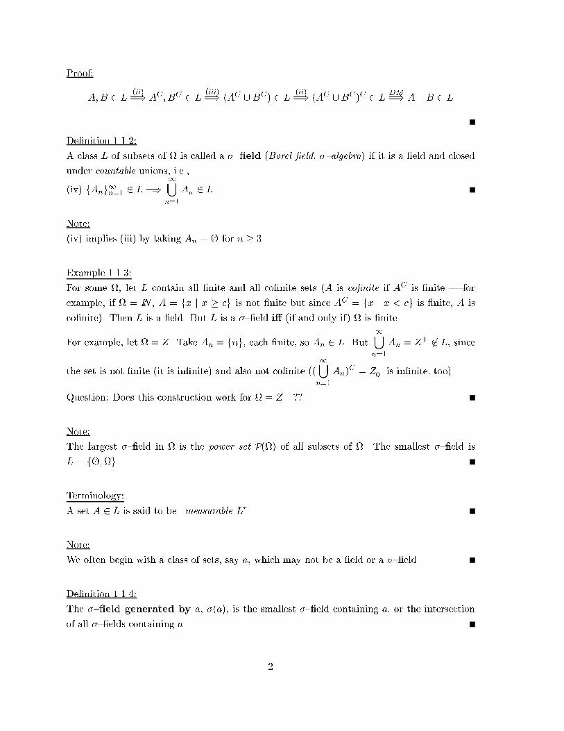
Proof:

A;B 2 L(ii)=) A

C; B

C 2 L(iii)=) (AC [BC) 2 L

(ii)=) (AC [BC)C 2 L

DM=) A \B 2 L

De�nition 1.1.2:

A class L of subsets of is called a �{�eld (Borel �eld, �{algebra) if it is a �eld and closed

under countable unions, i.e.,

(iv) fAng1n=1 2 L =)1[n=1

An 2 L.

Note:

(iv) implies (iii) by taking An = � for n � 3.

Example 1.1.3:

For some , let L contain all �nite and all co�nite sets (A is co�nite if AC is �nite | for

example, if = IN , A = fx j x � cg is not �nite but since AC = fx j x < cg is �nite, A is

co�nite). Then L is a �eld. But L is a �{�eld i� (if and only if) is �nite.

For example, let = Z. Take An = fng, each �nite, so An 2 L. But1[n=1

An = Z+ 62 L, since

the set is not �nite (it is in�nite) and also not co�nite ((1[n=1

An)C = Z

�0 is in�nite, too).

Question: Does this construction work for = Z+ ??

Note:

The largest �{�eld in is the power set P() of all subsets of . The smallest �{�eld is

L = f�;g.

Terminology:

A set A 2 L is said to be \measurable L".

Note:

We often begin with a class of sets, say a, which may not be a �eld or a �{�eld.

De�nition 1.1.4:

The �{�eld generated by a, �(a), is the smallest �{�eld containing a, or the intersection

of all �{�elds containing a.

2

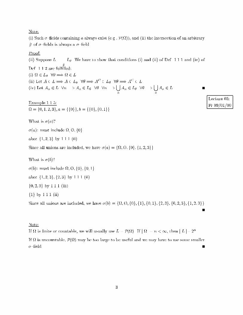
Note:

(i) Such �{�elds containing a always exist (e.g., P()), and (ii) the intersection of an arbitrary

# of �{�elds is always a �{�eld.

Proof:

(ii) Suppose L =\�

L�. We have to show that conditions (i) and (ii) of Def. 1.1.1 and (iv) of

Def. 1.1.2 are ful�lled:

(i) 2 L� 8� =) 2 L

(ii) Let A 2 L =) A 2 L� 8� =) AC 2 L� 8� =) A

C 2 L

(iv) Let An 2 L 8n =) An 2 L� 8� 8n =)[n

An 2 L� 8� =)[n

An 2 L

Lecture 03:

Fr 09/01/00Example 1.1.5:

= f0; 1; 2; 3g; a = ff0gg; b = ff0g; f0; 1gg.

What is �(a)?

�(a): must include ;�; f0g

also: f1; 2; 3g by 1.1.1 (ii)

Since all unions are included, we have �(a) = f;�; f0g; f1; 2; 3gg

What is �(b)?

�(b): must include ;�; f0g; f0; 1g

also: f1; 2; 3g; f2; 3g by 1.1.1 (ii)

f0; 2; 3g by 1.1.1 (iii)

f1g by 1.1.1 (ii)

Since all unions are included, we have �(b) = f;�; f0g; f1g; f0; 1g; f2; 3g; f0; 2; 3g; f1; 2; 3gg

Note:

If is �nite or countable, we will usually use L = P(). If j j= n <1, then j L j= 2n.

If is uncountable, P() may be too large to be useful and we may have to use some smaller

�{�eld.

3

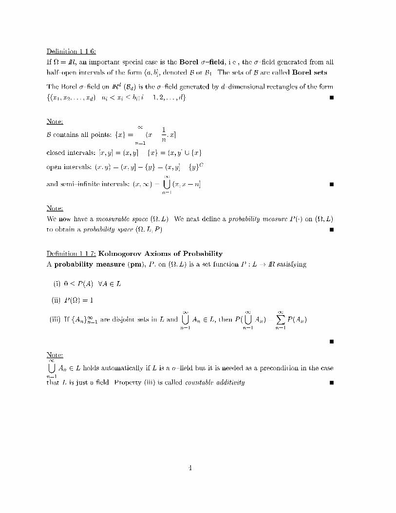
De�nition 1.1.6:

If = IR, an important special case is the Borel �{�eld, i.e., the �{�eld generated from all

half{open intervals of the form (a; b], denoted B or B1. The sets of B are called Borel sets.

The Borel �{�eld on IRd (Bd) is the �{�eld generated by d{dimensional rectangles of the form

f(x1; x2; : : : ; xd) j ai < xi � bi; i = 1; 2; : : : ; dg.

Note:

B contains all points: fxg =1\n=1

(x� 1

n; x]

closed intervals: [x; y] = (x; y] + fxg = (x; y] [ fxg

open intervals: (x; y) = (x; y]� fyg = (x; y] \ fygC

and semi{in�nite intervals: (x;1) =1[n=1

(x; x+ n]

Note:

We now have a measurable space (; L). We next de�ne a probability measure P (�) on (; L)

to obtain a probability space (; L; P ).

De�nition 1.1.7: Kolmogorov Axioms of Probability

A probability measure (pm), P , on (; L) is a set function P : L! IR satisfying

(i) 0 � P (A) 8A 2 L

(ii) P () = 1

(iii) If fAng1n=1 are disjoint sets in L and1[n=1

An 2 L, then P (1[n=1

An) =1Xn=1

P (An).

Note:1[n=1

An 2 L holds automatically if L is a �{�eld but it is needed as a precondition in the case

that L is just a �eld. Property (iii) is called countable additivity.

4

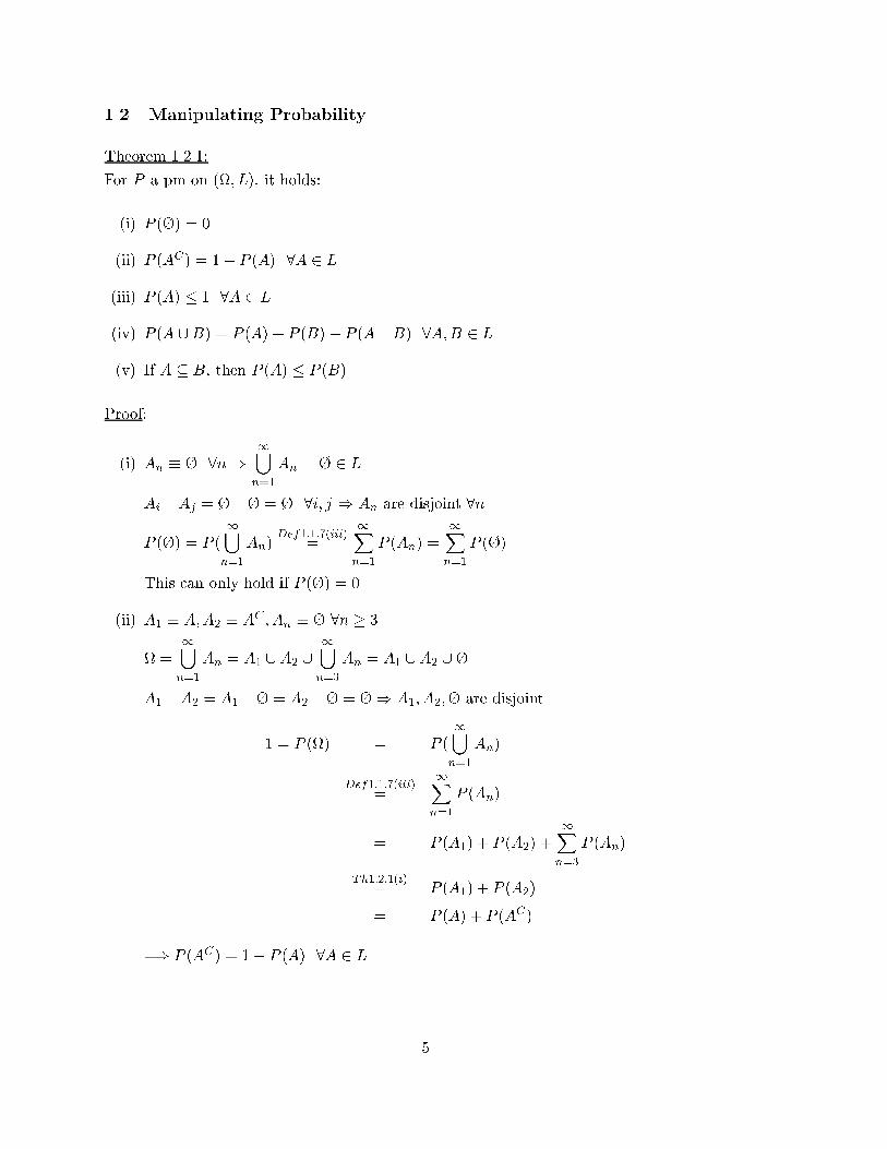
1.2 Manipulating Probability

Theorem 1.2.1:

For P a pm on (; L), it holds:

(i) P (�) = 0

(ii) P (AC) = 1� P (A) 8A 2 L

(iii) P (A) � 1 8A 2 L

(iv) P (A [B) = P (A) + P (B)� P (A \B) 8A;B 2 L

(v) If A � B, then P (A) � P (B).

Proof:

(i) An � � 8n)1[n=1

An = � 2 L.

Ai \Aj = � \� = � 8i; j ) An are disjoint 8n.

P (�) = P (1[n=1

An)Def1:1:7(iii)

=1Xn=1

P (An) =1Xn=1

P (�)

This can only hold if P (�) = 0.

(ii) A1 � A;A2 � AC; An � � 8n � 3.

=1[n=1

An = A1 [A2 [1[n=3

An = A1 [A2 [�.

A1 \A2 = A1 \� = A2 \� = �) A1; A2;� are disjoint.

1 = P () = P (1[n=1

An)

Def1:1:7(iii)=

1Xn=1

P (An)

= P (A1) + P (A2) +1Xn=3

P (An)

Th1:2:1(i)= P (A1) + P (A2)

= P (A) + P (AC)

=) P (AC) = 1� P (A) 8A 2 L.

5

(iii) By Th. 1.2.1 (ii) P (A) = 1� P (AC)

=) P (A) � 1 8A 2 L since P (AC) � 0 by Def. 1.1.7 (i).

(iv) A [ B = (A \ BC) [ (A \ B) [ (B \ A

C). So, (A [ B) can be written as a union of

disjoint sets (A \BC); (A \B); (B \AC):

=) P (A [B) = P ((A \BC) [ (A \B) [ (B \AC))

Def:1:1:7(iii)= P (A \BC) + P (A \B) + P (B \AC)

= P (A \BC) + P (A \B) + P (B \AC) + P (A \B)� P (A \B)

= (P (A \BC) + P (A \B)) + (P (B \AC) + P (A \B))� P (A \B)Def:1:1:7(iii)

= P (A) + P (B)� P (A \B)

Lecture 04:

We 09/06/00(v) B = (B \AC) [A where (B \AC) and A are disjoint sets.

P (B) = P ((B \AC) [A) Def1:1:7(iii)= P (B \AC) + P (A)

=) P (A) = P (B)� P (B \AC)

=) P (A) � P (B) since P (B \AC) � 0 by Def. 1.1.7 (i).

Theorem 1.2.2: Principle of Inclusion{Exclusion

Let A1; A2; : : : ; An 2 L. Then

P (n[

k=1

Ak) =nX

k=1

P (Ak)�nX

k1<k2

P (Ak1\Ak2)+nX

k1<k2<k3

P (Ak1\Ak2\Ak3)�: : :+(�1)n+1P (n\

k=1

Ak)

Proof:

n = 1 is trivial

n = 2 is Theorem 1.2.1 (iv)

Use induction for higher n (Homework).

Note:

A proof by induction consists of two steps:

First, we have to establish the induction base. For example, if we state that something

holds for all non{negative integers, then we have to show that it holds for n = 0. Similarly, if

we state that something holds for all integers, then we have to show that it holds for n = 1.

Formally, it is su�cient to verify a claim for the smallest valid integer only. However, to get

some feeling how the proof from n to n+ 1 might work, it is sometimes bene�cial to verify a

claim for 1; 2; or 3 as well.

6

In the second step, we have to establish the result in the induction step, showing that some-

thing holds for n + 1, using the fact that it holds for n (alternatively, we can show that it

holds for n, using the fact that it holds for n� 1).

Theorem 1.2.3: Bonferroni's Inequality

Let A1; A2; : : : ; An 2 L. Then

nXi=1

P (Ai)�Xi<j

P (Ai \Aj) � P (n[i=1

Ai) �nXi=1

P (Ai)

Proof:

Right side: P (n[i=1

Ai) �nXi=1

P (Ai)

Induction Base:

For n = 1, the right side evaluates to P (A1) � P (A1), which is true.

Formally, the next step is not required. However, it does not harm to verify the claim for

n = 2 as well. For n = 2, the right side evaluates to P (A1 [A2) � P (A1) + P (A2).

P (A1 [A2)Th:1:2:1(iv)

= P (A1) + P (A2) � P (A1 \ A2) � P (A1) + P (A2) since P (A1 \ A2) � 0

by Def. 1.1.7 (i).

This establishes the induction base for the right side.

Induction Step:

We assume the right side is true for n and show that it is true for n+ 1:

P (n+1[i=1

Ai) = P ((n[i=1

Ai) [An+1)

Th:1:2:1(iv)= P (

n[i=1

Ai) + P (An+1)� P ((n[i=1

Ai) \An+1)

Def:1:1:7(i)

� P (n[i=1

Ai) + P (An+1)

I:B:�

nXi=1

P (Ai) + P (An+1)

=n+1Xi=1

P (Ai)

Left side:nXi=1

P (Ai)�Xi<j

P (Ai \Aj) � P (n[i=1

Ai)

Induction Base:

For n = 1, the left side evaluates to P (A1) � P (A1), which is true.

7

For n = 2, the left side evaluates to P (A1)+P (A2)�P (A1 \A2) � P (A1 [A2), which is true

by Th. 1.2.1 (iv).

For n = 3, the left side evaluates to

P (A1) + P (A2) + P (A3)� P (A1 \A2)� P (A1 \A3)� P (A2 \A3) � P (A1 [A2 [A3).

This holds since

P (A1 [A2 [A3)

= P ((A1 [A2) [A3)

Th:1:2:1(iv)= P (A1 [A2) + P (A3)� P ((A1 [A2) \A3)

= P (A1 [A2) + P (A3)� P ((A1 \A3) [ (A2 \A3))

Th:1:2:1(iv)= P (A1) + P (A2)� P (A1 \A2) + P (A3)� P (A1 \A3)� P (A2 \A3)

+P ((A1 \A3) \ (A2 \A3))

= P (A1)+P (A2)+P (A3)�P (A1\A2)�P (A1 \A3)�P (A2\A3)+P (A1 \A2\A3)

Def1:1:7(i)

� P (A1) + P (A2) + P (A3)� P (A1 \A2)� P (A1 \A3)� P (A2 \A3)

This establishes the induction base for the left side.

Induction Step:

We assume the left side is true for n and show that it is true for n+ 1:

P (n+1[i=1

Ai) = P ((n[i=1

Ai) [An+1)

= P (n[i=1

Ai) + P (An+1)� P ((n[i=1

Ai) \An+1)

left I:B:

�nXi=1

P (Ai)�nXi<j

P (Ai \Aj) + P (An+1)� P ((n[i=1

Ai) \An+1)

=n+1Xi=1

P (Ai)�nXi<j

P (Ai \Aj)� P (n[i=1

(Ai \An+1))

Th:1:2:3 right side

�n+1Xi=1

P (Ai)�nXi<j

P (Ai \Aj)�nXi=1

P (Ai \An+1)

=n+1Xi=1

P (Ai)�n+1Xi<j

P (Ai \Aj)

8

Theorem 1.2.4: Boole's Inequality

Let A;B 2 L. Then

(i) P (A \B) � P (A) + P (B)� 1

(ii) P (A \B) � 1� P (AC)� P (BC)

Proof:

Homework

De�nition 1.2.5: Continuity of sets

For a sequence of sets fAng1n=1; An 2 L and A 2 L, we say

(i) An " A if A1 � A2 � A3 � : : : and A =1[n=1

An.

(ii) An # A if A1 � A2 � A3 � : : : and A =1\n=1

An.

Theorem 1.2.6:

If fAng1n=1; An 2 L and A 2 L, then limn!1P (An) = P (A) if 1.2.5 (i) or 1.2.5 (ii) holds.

Proof:

Part (i): Assume that 1.2.5 (i) holds.

Let B1 = A1 and Bk = Ak �Ak�1 = Ak \ACk�1 8k � 2

By construction, Bi \Bj = � for i 6= j

It is A =1[n=1

An =1[n=1

Bn

and also An =n[i=1

Ai =n[i=1

Bi

P(A) = P(1[k=1

Bk )Def. 1.1.7 (iii)

=1Xk=1

P (Bk) = limn!1[

nXk=1

P (Bk)]

Def. 1.1.7 (iii)= lim

n!1[P (n[

k=1

Bk)] = limn!1[P (

n[k=1

Ak)] = limn!1P (An)

The last step is possible since An =n[

k=1

Ak

9

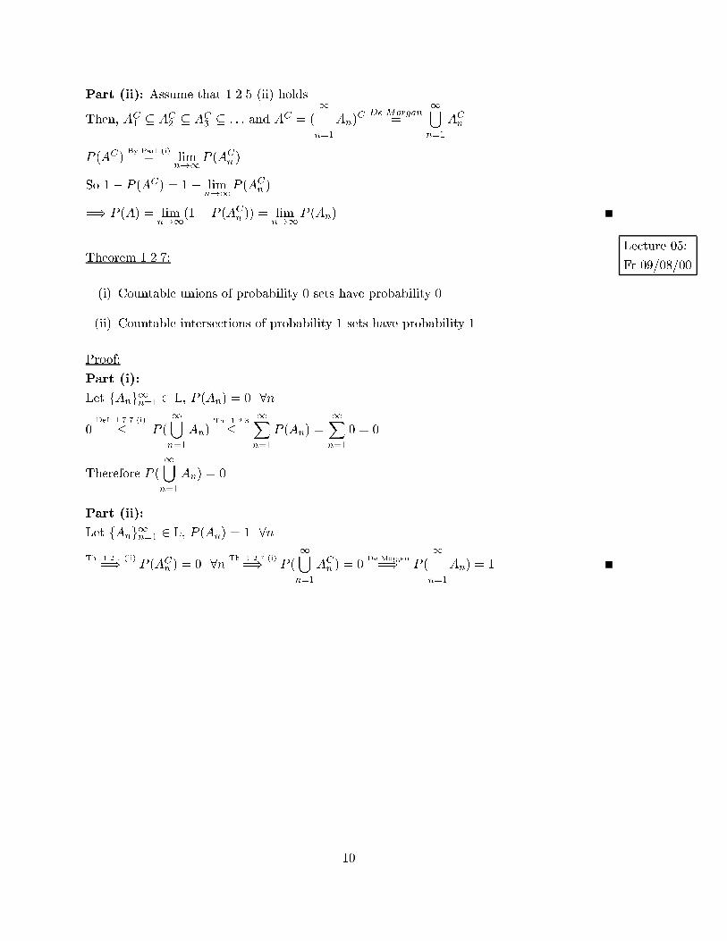
Part (ii): Assume that 1.2.5 (ii) holds.

Then, AC1 � A

C2 � A

C3 � : : : and A

C = (1\n=1

An)C De Morgan

=1[n=1

ACn

P (AC)By Part (i)

= limn!1P (AC

n )

So 1� P (AC) = 1� limn!1P (AC

n )

=) P (A) = limn!1(1� P (AC

n )) = limn!1P (An)

Lecture 05:

Fr 09/08/00Theorem 1.2.7:

(i) Countable unions of probability 0 sets have probability 0.

(ii) Countable intersections of probability 1 sets have probability 1.

Proof:

Part (i):

Let fAng1n=1 2 L, P (An) = 0 8n

0Def. 1.7.7 (i)

� P (1[n=1

An)Th. 1.2.3

�1Xn=1

P (An) =1Xn=1

0 = 0

Therefore P (1[n=1

An) = 0.

Part (ii):

Let fAng1n=1 2 L, P (An) = 1 8n

Th. 1.2.1 (ii)=) P (AC

n ) = 0 8n Th. 1.2.7 (i)=) P (

1[n=1

ACn ) = 0

De Morgan=) P (

1\n=1

An) = 1

10

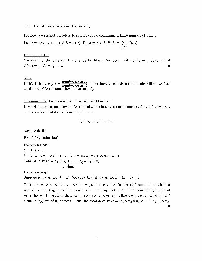
1.3 Combinatorics and Counting

For now, we restrict ourselves to sample spaces containing a �nite number of points.

Let = f!1; : : : ; !ng and L = P(). For any A 2 L;P (A) =X!j2A

P (!j).

De�nition 1.3.1:

We say the elements of are equally likely (or occur with uniform probability) if

P (!j) =1n8j = 1; : : : ; n.

Note:

If this is true, P (A) =number !j in A

number !j in . Therefore, to calculate such probabilities, we just

need to be able to count elements accurately.

Theorem 1.3.2: Fundamental Theorem of Counting

If we wish to select one element (a1) out of n1 choices, a second element (a2) out of n2 choices,

and so on for a total of k elements, there are

n1 � n2 � n3 � : : : � nk

ways to do it.

Proof: (By Induction)

Induction Base:

k = 1: trivial

k = 2: n1 ways to choose a1. For each, n2 ways to choose a2.

Total # of ways = n2 + n2 + : : :+ n2| {z }n1 times

= n1 � n2.

Induction Step:

Suppose it is true for (k � 1). We show that it is true for k = (k � 1) + 1.

There are n1 � n2 � n3 � : : : � nk�1 ways to select one element (a1) out of n1 choices, a

second element (a2) out of n2 choices, and so on, up to the (k � 1)th element (ak�1) out of

nk�1 choices. For each of these n1 � n2 � n3 � : : :� nk�1 possible ways, we can select the kth

element (ak) out of nk choices. Thus, the total # of ways = (n1�n2�n3� : : :� nk�1)� nk.

11

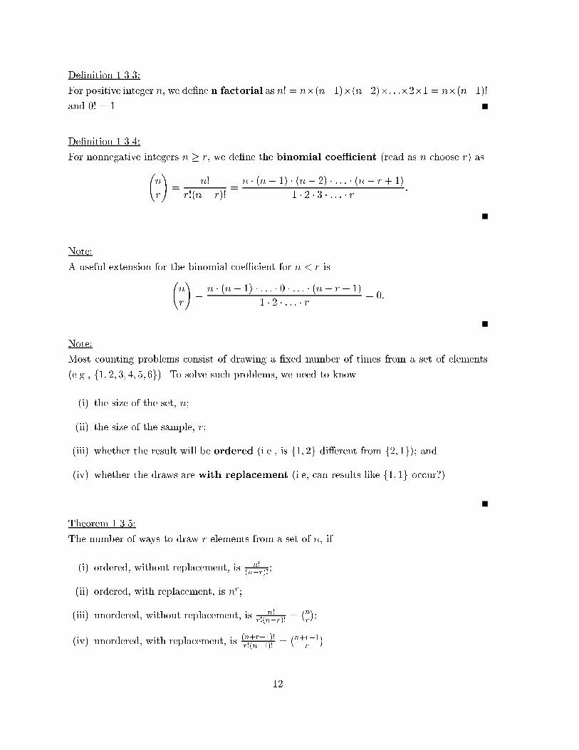
De�nition 1.3.3:

For positive integer n, we de�ne n factorial as n! = n�(n�1)�(n�2)�: : :�2�1 = n�(n�1)!and 0! = 1.

De�nition 1.3.4:

For nonnegative integers n � r, we de�ne the binomial coe�cient (read as n choose r) as

n

r

!=

n!

r!(n� r)!=

n � (n� 1) � (n� 2) � : : : � (n� r + 1)

1 � 2 � 3 � : : : � r :

Note:

A useful extension for the binomial coe�cient for n < r is n

r

!=

n � (n� 1) � : : : � 0 � : : : � (n� r + 1)

1 � 2 � : : : � r = 0:

Note:

Most counting problems consist of drawing a �xed number of times from a set of elements

(e.g., f1; 2; 3; 4; 5; 6g). To solve such problems, we need to know

(i) the size of the set, n;

(ii) the size of the sample, r;

(iii) whether the result will be ordered (i.e., is f1; 2g di�erent from f2; 1g); and

(iv) whether the draws are with replacement (i.e, can results like f1; 1g occur?).

Theorem 1.3.5:

The number of ways to draw r elements from a set of n, if

(i) ordered, without replacement, is n!(n�r)! ;

(ii) ordered, with replacement, is nr;

(iii) unordered, without replacement, is n!r!(n�r)! =

�nr

�;

(iv) unordered, with replacement, is(n+r�1)!r!(n�1)! =

�n+r�1r

�.

12

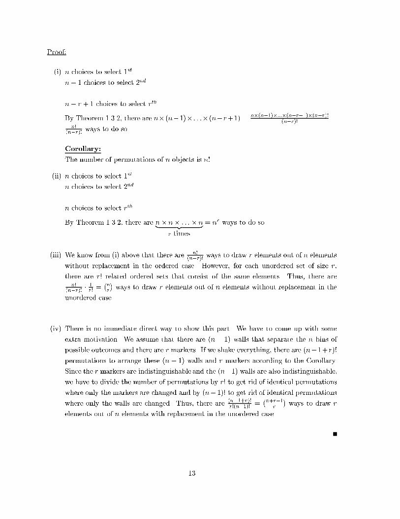
Proof:

(i) n choices to select 1st

n� 1 choices to select 2nd...

n� r + 1 choices to select rth

By Theorem 1.3.2, there are n� (n�1)� : : :� (n�r+1) =n�(n�1)�:::�(n�r+1)�(n�r)!

(n�r)! =n!

(n�r)! ways to do so.

Corollary:

The number of permutations of n objects is n!.

(ii) n choices to select 1st

n choices to select 2nd...

n choices to select rth

By Theorem 1.3.2, there are n� n� : : :� n| {z }r times

= nr ways to do so.

(iii) We know from (i) above that there are n!(n�r)! ways to draw r elements out of n elements

without replacement in the ordered case. However, for each unordered set of size r,

there are r! related ordered sets that consist of the same elements. Thus, there aren!

(n�r)! �1r! =

�nr

�ways to draw r elements out of n elements without replacement in the

unordered case.

(iv) There is no immediate direct way to show this part. We have to come up with some

extra motivation. We assume that there are (n � 1) walls that separate the n bins of

possible outcomes and there are r markers. If we shake everything, there are (n�1+r)!

permutations to arrange these (n � 1) walls and r markers according to the Corollary.

Since the r markers are indistinguishable and the (n�1) walls are also indistinguishable,we have to divide the number of permutations by r! to get rid of identical permutations

where only the markers are changed and by (n� 1)! to get rid of identical permutations

where only the walls are changed. Thus, there are(n�1+r)!r!(n�1)! =

�n+r�1r

�ways to draw r

elements out of n elements with replacement in the unordered case.

13

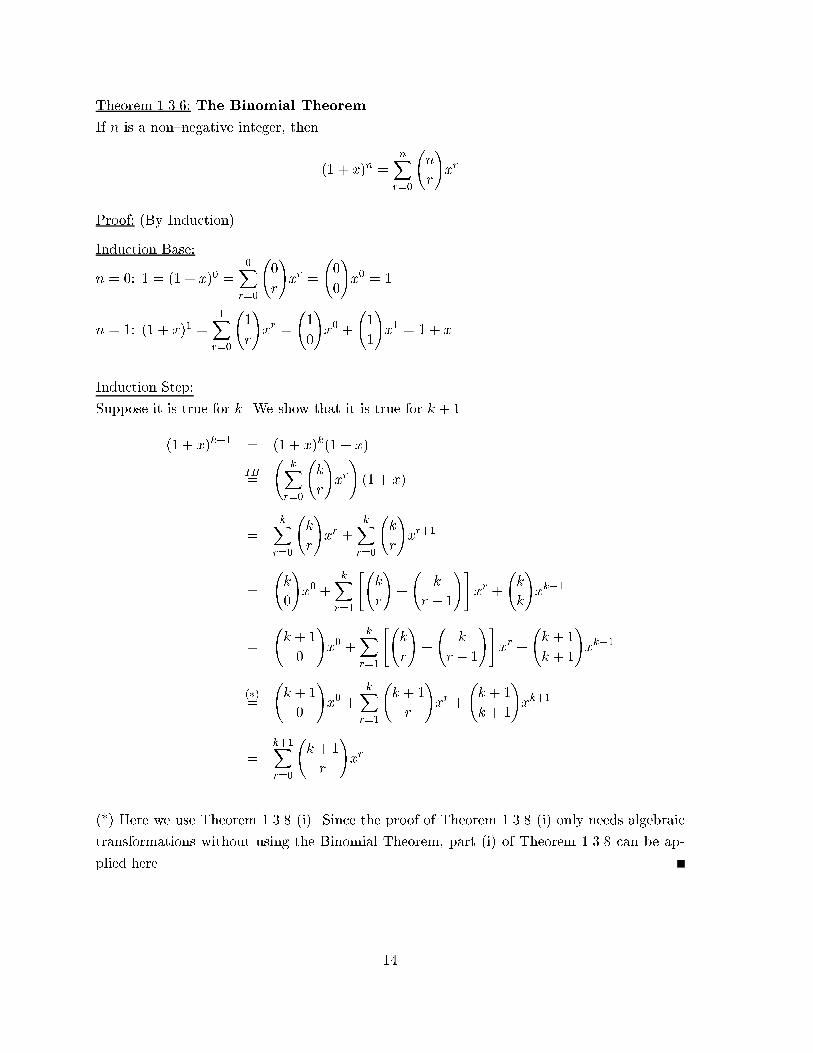
Theorem 1.3.6: The Binomial Theorem

If n is a non{negative integer, then

(1 + x)n =nX

r=0

n

r

!xr

Proof: (By Induction)

Induction Base:

n = 0: 1 = (1 + x)0 =0X

r=0

0

r

!xr =

0

0

!x0 = 1

n = 1: (1 + x)1 =1X

r=0

1

r

!xr =

1

0

!x0 +

1

1

!x1 = 1 + x

Induction Step:

Suppose it is true for k. We show that it is true for k + 1.

(1 + x)k+1 = (1 + x)k(1 + x)

IB=

kX

r=0

k

r

!xr

!(1 + x)

=kX

r=0

k

r

!xr +

kXr=0

k

r

!xr+1

=

k

0

!x0 +

kXr=1

" k

r

!+

k

r � 1

!#xr +

k

k

!xk+1

=

k + 1

0

!x0 +

kXr=1

" k

r

!+

k

r � 1

!#xr +

k + 1

k + 1

!xk+1

(�)=

k + 1

0

!x0 +

kXr=1

k + 1

r

!xr +

k + 1

k + 1

!xk+1

=k+1Xr=0

k + 1

r

!xr

(*) Here we use Theorem 1.3.8 (i). Since the proof of Theorem 1.3.8 (i) only needs algebraic

transformations without using the Binomial Theorem, part (i) of Theorem 1.3.8 can be ap-

plied here.

14

Lecture 06:

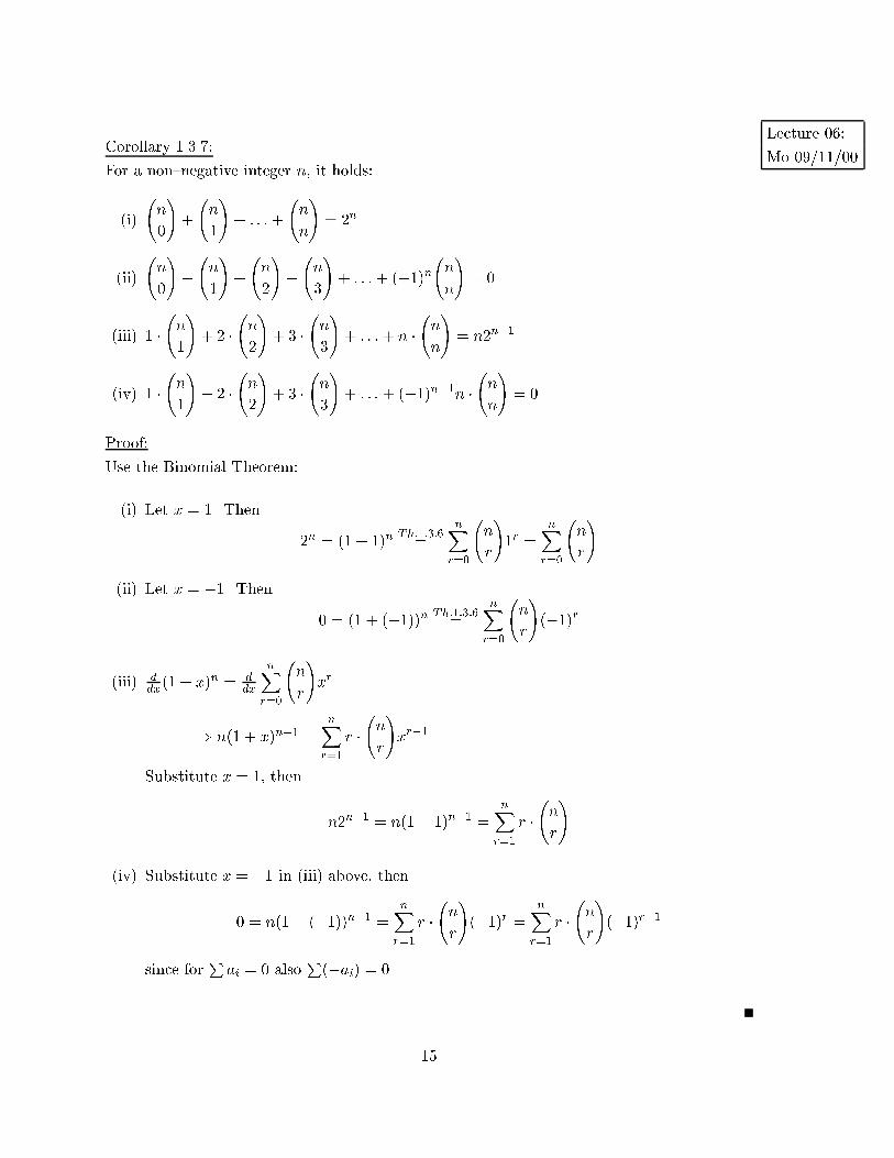
Mo 09/11/00Corollary 1.3.7:

For a non{negative integer n, it holds:

(i)

n

0

!+

n

1

!+ : : :+

n

n

!= 2n

(ii)

n

0

!� n

1

!+

n

2

!� n

3

!+ : : :+ (�1)n

n

n

!= 0

(iii) 1 � n

1

!+ 2 �

n

2

!+ 3 �

n

3

!+ : : :+ n �

n

n

!= n2n�1

(iv) 1 � n

1

!� 2 �

n

2

!+ 3 �

n

3

!+ : : :+ (�1)n�1n �

n

n

!= 0

Proof:

Use the Binomial Theorem:

(i) Let x = 1. Then

2n = (1 + 1)nTh:1:3:6=

nXr=0

n

r

!1r =

nXr=0

n

r

!

(ii) Let x = �1. Then

0 = (1 + (�1))n Th:1:3:6=

nXr=0

n

r

!(�1)r

(iii) ddx(1 + x)n = d

dx

nXr=0

n

r

!xr

=) n(1 + x)n�1 =nX

r=1

r � n

r

!xr�1

Substitute x = 1, then

n2n�1 = n(1 + 1)n�1 =nX

r=1

r � n

r

!

(iv) Substitute x = �1 in (iii) above, then

0 = n(1 + (�1))n�1 =nXr=1

r � n

r

!(�1)r =

nXr=1

r � n

r

!(�1)r�1

since forPai = 0 also

P(�ai) = 0.

15

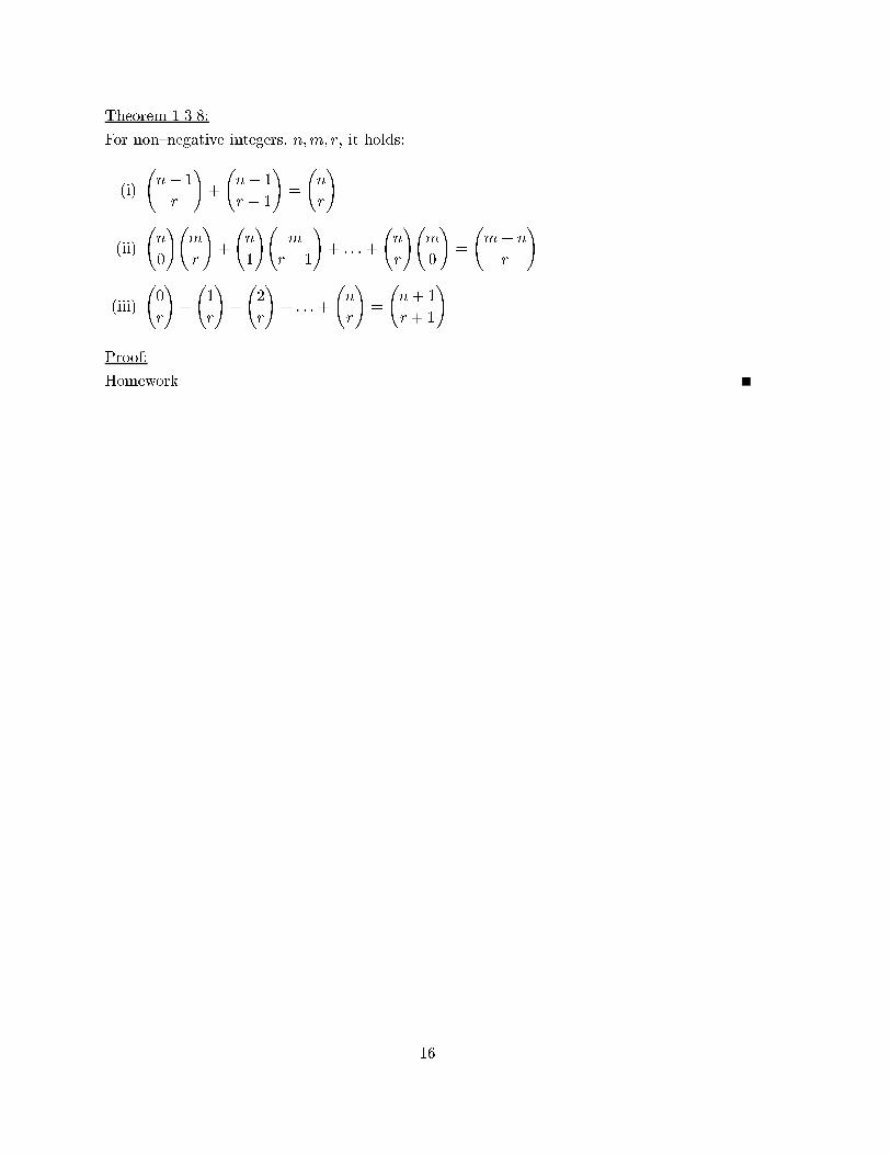
Theorem 1.3.8:

For non{negative integers, n;m; r, it holds:

(i)

n� 1

r

!+

n� 1

r � 1

!=

n

r

!

(ii)

n

0

! m

r

!+

n

1

! m

r � 1

!+ : : : +

n

r

! m

0

!=

m+ n

r

!

(iii)

0

r

!+

1

r

!+

2

r

!+ : : : +

n

r

!=

n+ 1

r + 1

!

Proof:

Homework

16

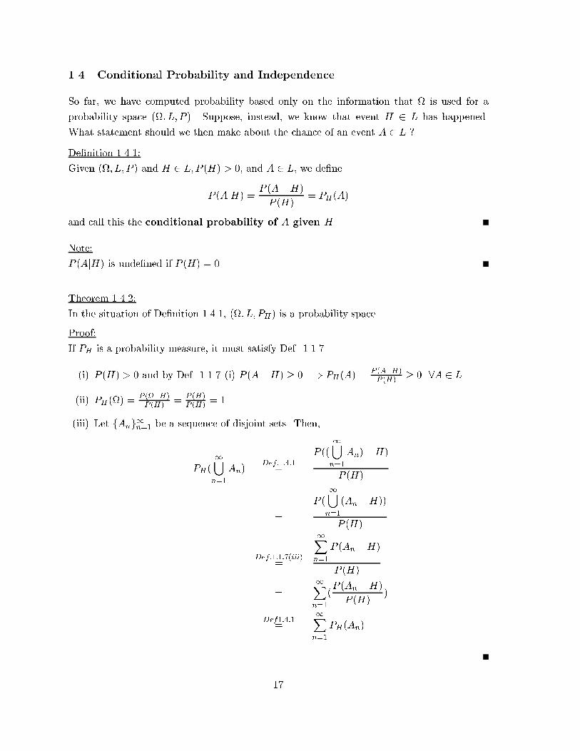
1.4 Conditional Probability and Independence

So far, we have computed probability based only on the information that is used for a

probability space (; L; P ). Suppose, instead, we know that event H 2 L has happened.

What statement should we then make about the chance of an event A 2 L ?

De�nition 1.4.1:

Given (; L; P ) and H 2 L;P (H) > 0, and A 2 L, we de�ne

P (AjH) =P (A \H)

P (H)= PH(A)

and call this the conditional probability of A given H.

Note:

P (AjH) is unde�ned if P (H) = 0.

Theorem 1.4.2:

In the situation of De�nition 1.4.1, (; L; PH ) is a probability space.

Proof:

If PH is a probability measure, it must satisfy Def. 1.1.7.

(i) P (H) > 0 and by Def. 1.1.7 (i) P (A \H) � 0 =) PH(A) =P (A\H)P (H) � 0 8A 2 L

(ii) PH() =P (\H)P (H) =

P (H)P (H) = 1

(iii) Let fAng1n=1 be a sequence of disjoint sets. Then,

PH(1[n=1

An)Def:1:4:1

=

P ((1[n=1

An) \H)

P (H)

=

P (1[n=1

(An \H))

P (H)

Def:1:1:7(iii)=

1Xn=1

P (An \H)

P (H)

=1Xn=1

(P (An \H)

P (H))

Def1:4:1=

1Xn=1

PH(An)

17

Note:

What we have done is to move to a new sample space H and a new �{�eld LH = L \H of

subsets A\H for A 2 L. We thus have a new measurable space (H; LH) and a new probability

space (H; LH ; PH).

Note:

From De�nition 1.4.1, if A;B 2 L;P (A) > 0, and P (B) > 0, then

P (A \B) = P (A)P (BjA) = P (B)P (AjB);

which generalizes to the following Theorem.

Theorem 1.4.3: Multiplication Rule

If A1; : : : ; An 2 L and P (n�1\j=1

Aj) > 0, then

P (n\j=1

Aj) = P (A1) � P (A2jA1) � P (A3jA1 \A2) � : : : � P (Anjn�1\j=1

Aj):

Proof:

Homework

De�nition 1.4.4:

A collection of subsets fAng1n=1 of form a partition of if

(i)1[n=1

An = , and

(ii) Ai \Aj = � 8i 6= j, i.e., elements are pairwise disjoint.

Theorem 1.4.5: Law of Total Probability

If fHjg1j=1 is a partition of , and P (Hj) > 0 8j, then, for A 2 L,

P (A) =1Xj=1

P (A \Hj) =1Xj=1

P (Hj)P (AjHj):

Proof:

By the Note preceding Theorem 1.4.3, the summands on both sides are equal

=) the right side of Th. 1.4.5 is true.

18

The left side proof:

Hj are disjoint ) A \Hj are disjoint

A = A \ Def1:4:4

= A \ (1[j=1

Hj) =1[j=1

(A \Hj)

=) P (A) = P (1[j=1

(A \Hj))Def1:1:7(iii)

=1Xj=1

P (A \Hj)

Lecture 07:

We 09/13/00Theorem 1.4.6: Bayes' Rule

Let fHjg1j=1 be a partition of , and P (Hj) > 0 8j. Let A 2 L and P (A) > 0. Then

P (HjjA) =P (Hj)P (AjHj)

1Xn=1

P (Hn)P (AjHn)

8j:

Proof:

P (Hj \A)Def1:4:1

= P (A) � P (HjjA) = P (Hj) � P (AjHj)

=) P (HjjA) = P (Hj)�P (AjHj)P (A)

Th:1:4:5=

P (Hj)�P (AjHj)1Xn=1

P (Hn)P (AjHn)

.

De�nition 1.4.7:

For A;B 2 L, A and B are independent i� P (A \B) = P (A)P (B).

Note:

� There are no restrictions on P (A) or P (B).

� If A and B are independent, then P (AjB) = P (A) (given that P (B) > 0) and P (BjA) =P (B) (given that P (A) > 0).

� If A and B are independent, then the following events are independent as well: A and

BC ; AC and B; AC and B

C .

De�nition 1.4.8:

Let A be a collection of L{sets. The events of A are pairwise independent i� for every

distinct A1; A2 2 A it holds P (A1 \A2) = P (A1)P (A2).

19

De�nition 1.4.9:

Let A be a collection of L{sets. The events of A are mutually independent (or completely

independent) i� for every �nite subcollection fAi1 ; : : : ; Aikg; Aij 2 A, it holds

P (k\

j=1

Aij ) =kY

j=1

P (Aij ):

Note:

To check for mutually independence of n events fA1; : : : ; Ang 2 L, there are 2n � n� 1 rela-

tions (i.e., all subcollections of size 2 or more) to check.

Example 1.4.10:

Flip a fair coin twice. = fHH;HT; TH; TTg.A1 = \H on 1st toss"

A2 = \H on 2nd toss"

A3 = \Exactly one H"

Obviously, P (A1) = P (A2) = P (A3) =12 .

Question: Are A1; A2 and A3 pairwise independent and also mutually independent?

P (A1 \A2) = :25 = :5 � :5 = P (A1) � P (A2)) A1; A2 are independent.

P (A1 \A3) = :25 = :5 � :5 = P (A1) � P (A3)) A1; A3 are independent.

P (A2 \A3) = :25 = :5 � :5 = P (A2) � P (A3)) A2; A3 are independent.

Thus, A1; A2; A3 are pairwise independent.

P (A1 \ A2 \ A3) = 0 6= :5 � :5 � :5 = P (A1) � P (A2) � P (A3) ) A1; A2; A3 are not mutually

independent.

Example 1.4.11: (from Rohatgi, page 37, Example 5)

� r students. 365 possible birthdays for each student that are equally likely.

� One student at a time is asked for his/her birthday.

� If one of the other students hears this birthday and it matches his/her birthday, this

other student has to raise his/her hand | if at least one other student raises his/her

hand, the procedure is over.

20

� We are interested in

pk = P (procedure terminates at the kth student)

= P (a hand is �rst risen when the kth student is asked for his/her birthday)

It is

p1 = P (at least 1 other from the (r � 1) students has a birthday on this particular day.)

= 1� P (all (r � 1) students have a birthday on the remaining 364 out of 365 days)

= 1��364

365

�r�1

p2 = P (no student has a birthday matching the �rst student and at least one

of the other (r � 2) students has a b-day matching the second student)

Let A � No student has a b-day matching the 1ststudent

Let B � At least one of the other (r � 2) has b-day matching 2nd

So p2 = P (A \B)

= P (A) � P (BjA)

= P (no student has a matching b-day with the 1ststudent )�

P (at least one of the remaining students has a matching b-day with the second,

given that no one matched the �rst.)

= (1� p1)[1 � P (all (r � 2) students have a b-day on the remaining 363 out of 364 days)

=

�364

365

�r�1 "1�

�363

364

�r�2#

=

�365 � 1

365

�r�1 "1�

�363

364

�r�2#(�)

=365

365

�1� 1

365

�r�1 "1�

�363

364

�r�2#

=

�365P2�1(365)2�1

��1� 2� 1

365

�r�2+1 "1�

�365� 2

365 � 2 + 1

�r�2#

Formally, we have to write this sequence of equalities in this order. However, it often might

be easier to �rst work from both sides towards a particular result and combine partial results

afterwards. Here, one might decide to stop at (�) with the \forward" direction of the equalities

21

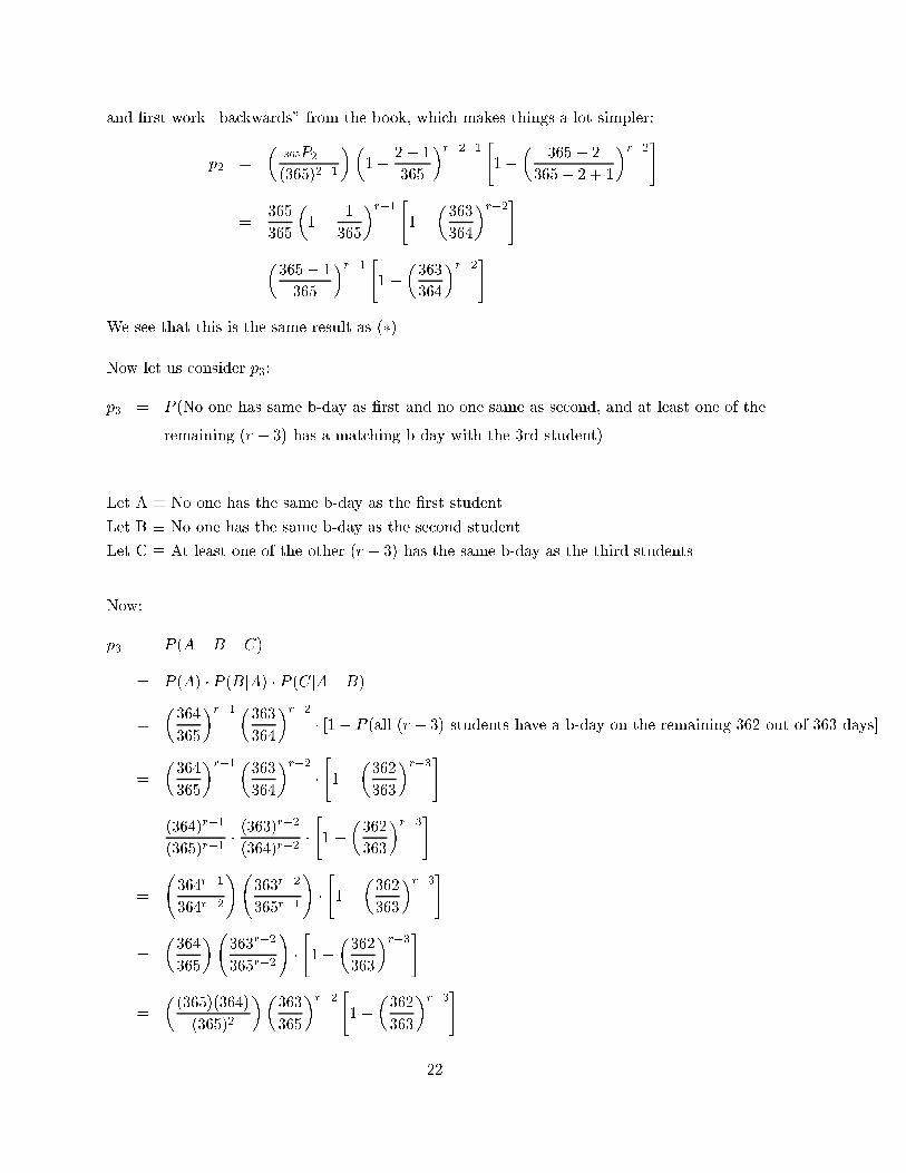
and �rst work \backwards" from the book, which makes things a lot simpler:

p2 =

�365P2�1(365)2�1

��1� 2� 1

365

�r�2+1 "1�

�365 � 2

365 � 2 + 1

�r�2#

=365

365

�1� 1

365

�r�1 "1�

�363

364

�r�2#

=

�365� 1

365

�r�1 "1�

�363

364

�r�2#

We see that this is the same result as (�).

Now let us consider p3:

p3 = P (No one has same b-day as �rst and no one same as second, and at least one of the

remaining (r � 3) has a matching b-day with the 3rd student)

Let A � No one has the same b-day as the �rst student

Let B � No one has the same b-day as the second student

Let C � At least one of the other (r � 3) has the same b-day as the third students

Now:

p3 = P (A \B \ C)

= P (A) � P (BjA) � P (CjA \B)

=

�364

365

�r�1 �363364

�r�2� [1� P (all (r � 3) students have a b-day on the remaining 362 out of 363 days]

=

�364

365

�r�1 �363364

�r�2�"1�

�362

363

�r�3#

=(364)r�1

(365)r�1� (363)

r�2

(364)r�2�"1�

�362

363

�r�3#

=

364r�1

364r�2

! 363r�2

365r�1

!�"1�

�362

363

�r�3#

=

�364

365

� 363r�2

365r�2

!�"1�

�362

363

�r�3#

=

�(365)(364)

(365)2

��363

365

�r�2 "1�

�362

363

�r�3#

22

=

�365P2

(365)2

��1� 2

365

�r�2 "1�

�362

363

�r�3#

=

�365P3�1(365)3�1

��1� 3� 1

365

�r�3+1 "1�

�365 � 3

365 � 3 + 1

�r�3#

Once again, working \backwards" from the book should help to better understand these

transformations.

For general pk and restrictions on r and k see Homework.

23

Lecture 08:

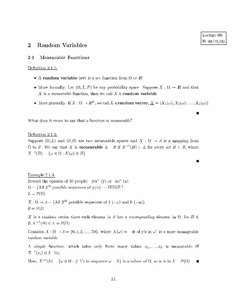
Fr 09/15/002 Random Variables

2.1 Measurable Functions

De�nition 2.1.1:

� A random variable (rv) is a set function from to IR.

� More formally: Let (; L; P ) be any probability space. Suppose X : ! IR and that

X is a measurable function, then we call X a random variable.

� More generally: IfX : ! IRk, we callX a random vector, X = (X1(!); X2(!); : : : ;Xk(!)).

What does it mean to say that a function is measurable?

De�nition 2.1.2:

Suppose (; L) and (S;B) are two measurable spaces and X : ! S is a mapping from

to S. We say that X is measurable L � B if X�1(B) 2 L for every set B 2 B, where

X�1(B) = f! 2 : X(!) 2 Bg.

Example 2.1.3:

Record the opinion of 50 people: \yes" (y) or \no" (n).

= fAll 250 possible sequences of y/ng | HUGE !

L = P()

X : ! S = fAll 250 possible sequences of 1 (=y) and 0 (=n)gB = P(S)

X is a random vector since each element in S has a corresponding element in , for B 2B; X�1(B) 2 L = P().

Consider X : ! S = f0; 1; 2; : : : ; 50g, where X(!) = \# of y's in !" is a more manageable

random variable.

A simple function, which takes only �nite many values x1; : : : ; xk is measurable i�

X�1(xi) 2 L 8xi.

Here, X�1(k) = f! 2 : # 1's in sequence ! = kg is a subset of , so it is in L = P()

24

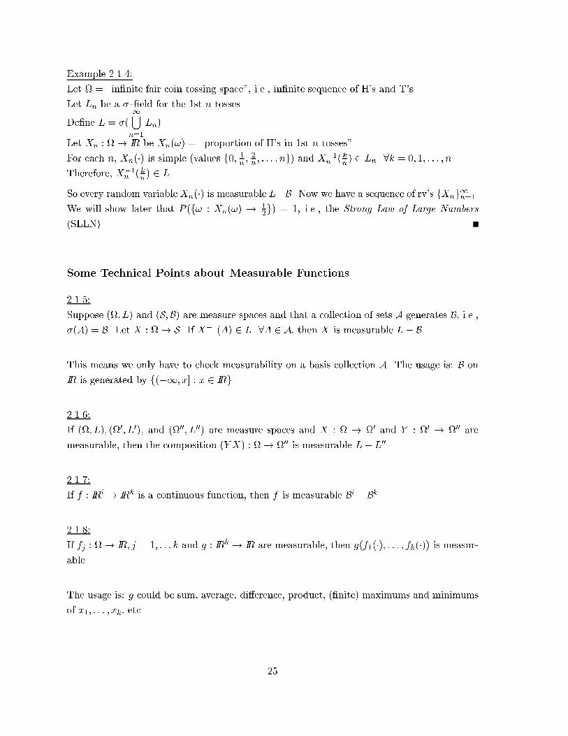
Example 2.1.4:

Let = \in�nite fair coin tossing space", i.e., in�nite sequence of H's and T's.

Let Ln be a �{�eld for the 1st n tosses.

De�ne L = �(1[n=1

Ln).

Let Xn : ! IR be Xn(!) = \proportion of H's in 1st n tosses".

For each n, Xn(�) is simple (values f0; 1n ;2n ; : : : ; ng) and X

�1n ( kn) 2 Ln 8k = 0; 1; : : : ; n.

Therefore, X�1n ( kn) 2 L.

So every random variable Xn(�) is measurable L�B. Now we have a sequence of rv's fXng1n=1.We will show later that P (f! : Xn(!) ! 1

2g) = 1, i.e., the Strong Law of Large Numbers

(SLLN).

Some Technical Points about Measurable Functions

2.1.5:

Suppose (; L) and (S;B) are measure spaces and that a collection of sets A generates B, i.e.,

�(A) = B. Let X : ! S. If X�1(A) 2 L 8A 2 A, then X is measurable L� B.

This means we only have to check measurability on a basis collection A. The usage is: B on

IR is generated by f(�1; x] : x 2 IRg.

2.1.6:

If (; L); (0; L0), and (00; L00) are measure spaces and X : ! 0 and Y : 0 ! 00 are

measurable, then the composition (Y X) : ! 00 is measurable L� L00.

2.1.7:

If f : IRi ! IRk is a continuous function, then f is measurable Bi � Bk.

2.1.8:

If fj : ! IR; j = 1; : : : k and g : IRk ! IR are measurable, then g(f1(�); : : : ; fk(�)) is measur-able.

The usage is: g could be sum, average, di�erence, product, (�nite) maximums and minimums

of x1; : : : ; xk, etc.

25

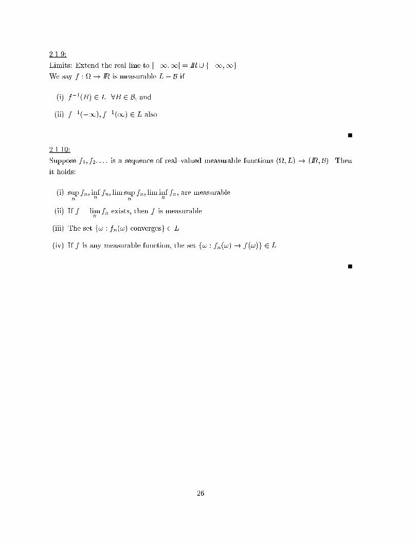
2.1.9:

Limits: Extend the real line to [�1;1] = IR [ f�1;1g.We say f : ! IR is measurable L� B if

(i) f�1(B) 2 L 8B 2 B, and

(ii) f�1(�1); f�1(1) 2 L also.

2.1.10:

Suppose f1; f2; : : : is a sequence of real{valued measurable functions (; L) ! (IR;B). Then

it holds:

(i) supnfn; inf

nfn; lim sup

nfn; lim inf

nfn, are measurable.

(ii) If f = limnfn exists, then f is measurable.

(iii) The set f! : fn(!) convergesg 2 L.

(iv) If f is any measurable function, the set f! : fn(!)! f(!)g 2 L.

26

2.2 Probability Distribution of a Random Variable

The de�nition of a random variable X : (; L) ! (S;B) makes no mention of P . We now

introduce a probability measure on (S;B).

Theorem 2.2.1:

A random variable X on (; L; P ) induces a probability measure on a space (IR;B; Q) with

the probability distribution Q of X de�ned by

Q(B) = P (X�1(B)) = P (f! : X(!) 2 Bg) 8B 2 B:

Note:

By the de�nition of a random variable, X�1(B) 2 L 8B 2 B. Q is called induced proba-

bility.

Proof:

If X induces a probability measure Q on (IR;B), then Q must satisfy the Kolmogorov Axioms

of probability.

X : (; L)! (S;B). X is a rv ) X�1(B) = f! : X(!) 2 Bg = A 2 L 8B 2 B.

(i) Q(B) = P (X�1(B)) = P (f! : X(!) 2 Bg) = P (A)Def:1:1:7(i)

� 0 8B 2 B

(ii) Q(IR) = P (X�1(IR)) X rv= P ()

Def:1:1:7(ii)= 1

(iii) Let fBng1n=1 2 B; Bi \Bj = � 8i 6= j. Then,

Q(1[n=1

Bn) = P (X�1(1[n=1

Bn))(�)= P (

1[n=1

(X�1(Bn)))Def:1:1:7(iii)

=1Xn=1

P (X�1(Bn)) =1Xn=1

Q(Bn)

(�) holds since X�1(�) commutes with unions/intersections and preserves disjointedness.

Lecture 09:

Mo 09/18/00De�nition 2.2.2:

A real{valued function F on (�1;1) that is non{decreasing, right{continuous, and satis�es

F (�1) = 0; F (1) = 1

is called a cumulative distribution function (cdf) on IR.

Note:

No mention of probability space or measure P in De�nition 2.2.2 above.

27

De�nition 2.2.3:

Let P be a probability measure on (IR;B). The cdf associated with P is

F (x) = FP (x) = P ((�1; x]) = P (f! : X(!) � xg) = P (X � x)

for a random variable X de�ned on (IR;B; P ).

Note:

F (�) de�ned as in De�nition 2.2.3 above indeed is a cdf.

Proof (of Note):

(i) Let x1 < x2

=) (�1; x1] � (�1; x2]

=) F (x1) = P (f! : X(!) � x1g)Th:1:2:1(v)

� P (f! : X(!) � x2g) = F (x2)

Thus, since x1 < x2 and F (x1) � F (x2), F (:) is non{decreasing.

(ii) Since F is non-decreasing, it is su�cient to show that F (:) is right{continuous if for any

sequence of numbers xn ! x+ (which means that xn is approaching x from the right)

with x1 > x2 > : : : > xn > : : : > x : F (xn)! F (x):

Let An = f! : X(!) 2 (x; xn]g 2 L and An # �. None of the intervals (x; xn] contains x.As xn ! x+, the number of points ! in An diminishes until the set is empty. Formally,

limn!1An = lim

n!1

n\i=1

Ai =1\n=1

An = �.

By Theorem 1.2.6 it follows that

limn!1P (An) = P ( lim

n!1An) = P (�) = 0.

It is

P (An) = P (f! : X(!) � xng)� P (f! : X(!) � xg) = F (xn)� F (x).

=) ( limn!1F (xn))� F (x) = lim

n!1(F (xn)� F (x)) = limn!1P (An) = 0

=) limn!1F (xn) = F (x)

=) F (x) is right{continuous.

28

(iii) F (�n) Def: 2:2:3= P (f! : X(!) � �ng)

=)F (�1) = lim

n!1F (�n)

= limn!1P (f! : X(!) � �ng)

= P ( limn!1f! : X(!) � �ng)

= P (�)

= 0

(iv) F (n)Def: 2:2:3

= P (f! : X(!) � ng)=)

F (1) = limn!1F (n)

= limn!1P (f! : X(!) � ng)

= P ( limn!1f! : X(!) � ng)

= P ()

= 1

Note that (iii) and (iv) implicitly use Theorem 1.2.6. In (iii), we use An = (�1;�n) whereAn � An+1 and An # �. In (iv), we use An = (�1; n) where An � An+1 and An " IR.

De�nition 2.2.4:

If a random variable X : ! IR has induced a probability measure PX on (IR;B) with cdf

F (x), we say

(i) rv X is continuous if F (x) is continuous in x.

(ii) rv X is discrete if F (x) is a step function in x.

Note:

There are rvs that are mixtures of continuous and discrete rvs. One such example is a trun-

cated failure time distribution. We assume a continuous distribution (e.g., exponential) up

to a given truncation point x and assign the \remaining" probability to the truncation point.

Thus, a single point has a probability > 0 and F (x) jumps at the truncation point x.

29

De�nition 2.2.5:

Two random variables X and Y are identically distributed i�

PX(X 2 A) = PY (Y 2 A) 8A 2 L:

Note:

Def. 2.2.5 does not mean that X(!) = Y (!) 8! 2 . For example,

X = # H in 3 coin tosses

Y = # T in 3 coin tosses

X;Y are both Bin(3; 0:5), i.e., identically distributed, but for ! = (H;H; T ); X(!) = 2 6= 1 =

Y (!), i.e., X 6= Y .

Theorem 2.2.6:

The following two statements are equivalent:

(i) X;Y are identically distributed.

(ii) FX(x) = FY (x) 8x 2 IR.

Proof:

(i) ) (ii):

FX(x) = PX((�1; x])

= P (f! : X(!) 2 (�1; x]g)byDef:2:2:5

= P (f! : Y (!) 2 (�1; x]g)

= PY ((�1; x])

= FY (X)

(ii) ) (i):

Requires extra knowledge from measure theory.

30

Lecture 10:

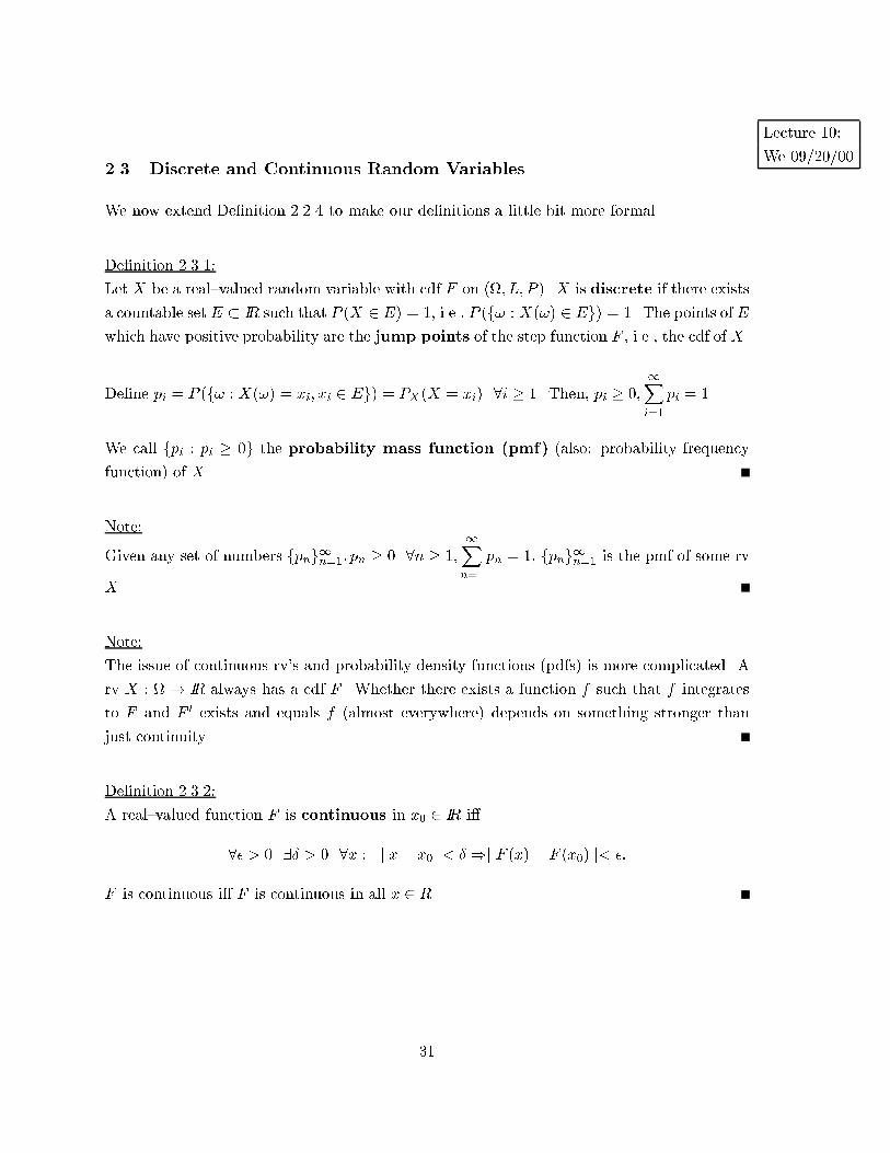
We 09/20/002.3 Discrete and Continuous Random Variables

We now extend De�nition 2.2.4 to make our de�nitions a little bit more formal.

De�nition 2.3.1:

Let X be a real{valued random variable with cdf F on (; L; P ). X is discrete if there exists

a countable set E � IR such that P (X 2 E) = 1, i.e., P (f! : X(!) 2 Eg) = 1. The points of E

which have positive probability are the jump points of the step function F , i.e., the cdf of X.

De�ne pi = P (f! : X(!) = xi; xi 2 Eg) = PX(X = xi) 8i � 1. Then, pi � 0;1Xi=1

pi = 1.

We call fpi : pi � 0g the probability mass function (pmf) (also: probability frequency

function) of X.

Note:

Given any set of numbers fpng1n=1; pn � 0 8n � 1;1Xn=1

pn = 1, fpng1n=1 is the pmf of some rv

X.

Note:

The issue of continuous rv's and probability density functions (pdfs) is more complicated. A

rv X : ! IR always has a cdf F . Whether there exists a function f such that f integrates

to F and F0 exists and equals f (almost everywhere) depends on something stronger than

just continuity.

De�nition 2.3.2:

A real{valued function F is continuous in x0 2 IR i�

8� > 0 9� > 0 8x : j x� x0 j< � )j F (x)� F (x0) j< �:

F is continuous i� F is continuous in all x 2 R.

31

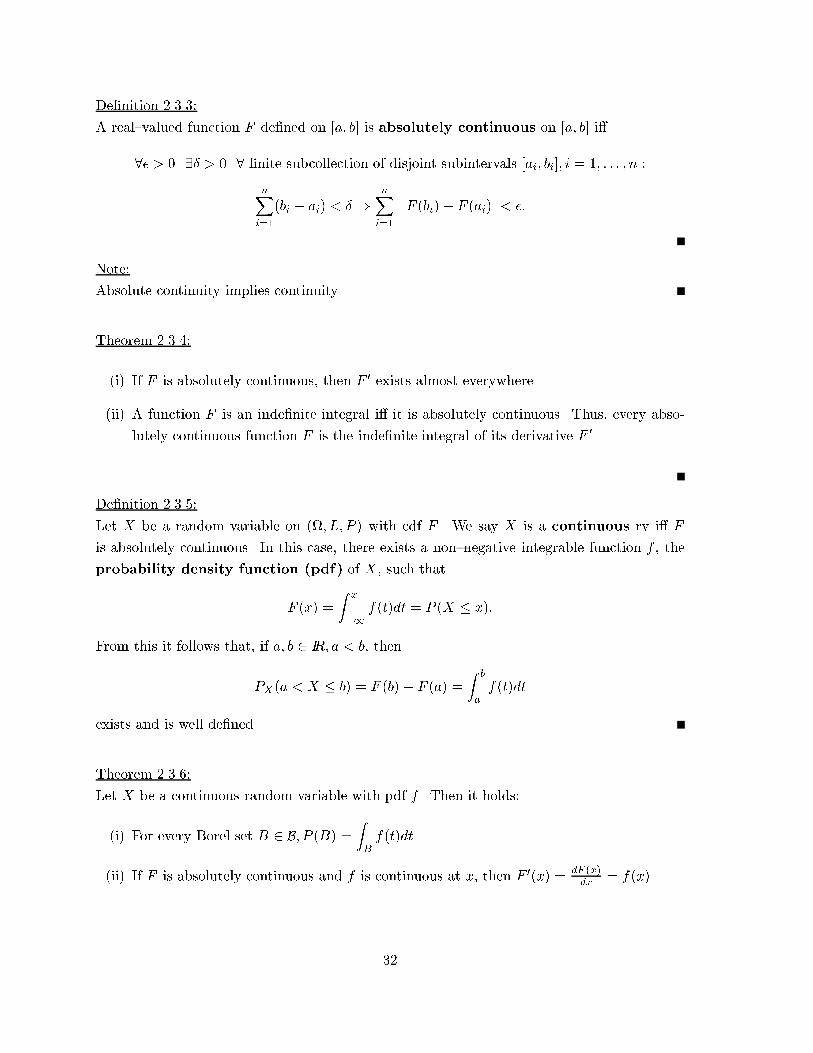
De�nition 2.3.3:

A real{valued function F de�ned on [a; b] is absolutely continuous on [a; b] i�

8� > 0 9� > 0 8 �nite subcollection of disjoint subintervals [ai; bi]; i = 1; : : : ; n :

nXi=1

(bi � ai) < � )nXi=1

j F (bi)� F (ai) j< �:

Note:

Absolute continuity implies continuity.

Theorem 2.3.4:

(i) If F is absolutely continuous, then F0 exists almost everywhere.

(ii) A function F is an inde�nite integral i� it is absolutely continuous. Thus, every abso-

lutely continuous function F is the inde�nite integral of its derivative F 0.

De�nition 2.3.5:

Let X be a random variable on (; L; P ) with cdf F . We say X is a continuous rv i� F

is absolutely continuous. In this case, there exists a non{negative integrable function f , the

probability density function (pdf) of X, such that

F (x) =

Z x

�1f(t)dt = P (X � x):

From this it follows that, if a; b 2 IR; a < b, then

PX(a < X � b) = F (b)� F (a) =

Z b

af(t)dt

exists and is well de�ned.

Theorem 2.3.6:

Let X be a continuous random variable with pdf f . Then it holds:

(i) For every Borel set B 2 B; P (B) =ZBf(t)dt.

(ii) If F is absolutely continuous and f is continuous at x, then F0(x) = dF (x)

dx = f(x).

32

Proof:

Part (i): From De�nition 2.3.5 above.

Part (ii): By Fundamental Theorem of Calculus.

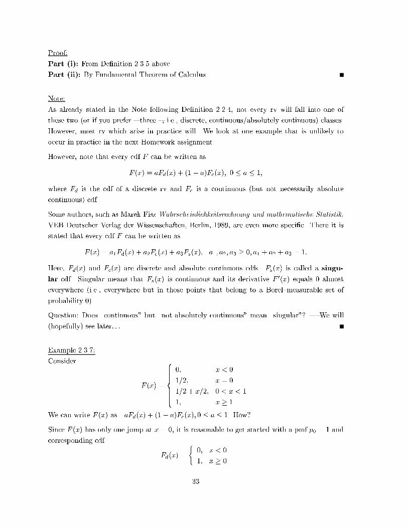
Note:

As already stated in the Note following De�nition 2.2.4, not every rv will fall into one of

these two (or if you prefer { three {, i.e., discrete, continuous/absolutely continuous) classes.

However, most rv which arise in practice will. We look at one example that is unlikely to

occur in practice in the next Homework assignment.

However, note that every cdf F can be written as

F (x) = aFd(x) + (1� a)Fc(x); 0 � a � 1;

where Fd is the cdf of a discrete rv and Fc is a continuous (but not necessarily absolute

continuous) cdf.

Some authors, such as Marek Fisz Wahrscheinlichkeitsrechnung und mathematische Statistik,

VEB Deutscher Verlag der Wissenschaften, Berlin, 1989, are even more speci�c. There it is

stated that every cdf F can be written as

F (x) = a1Fd(x) + a2Fc(x) + a3Fs(x); a1; a2; a3 � 0; a1 + a2 + a3 = 1:

Here, Fd(x) and Fc(x) are discrete and absolute continuous cdfs. Fs(x) is called a singu-

lar cdf. Singular means that Fs(x) is continuous and its derivative F0(x) equals 0 almost

everywhere (i.e., everywhere but in those points that belong to a Borel{measurable set of

probability 0).

Question: Does \continuous" but \not absolutely continuous" mean \singular"? | We will

(hopefully) see later: : :

Example 2.3.7:

Consider

F (x) =

8>>>>><>>>>>:

0; x < 0

1=2; x = 0

1=2 + x=2; 0 < x < 1

1; x � 1

We can write F (x) as aFd(x) + (1� a)Fc(x); 0 � a � 1. How?

Since F (x) has only one jump at x = 0, it is reasonable to get started with a pmf p0 = 1 and

corresponding cdf

Fd(x) =

(0; x < 0

1; x � 0

33

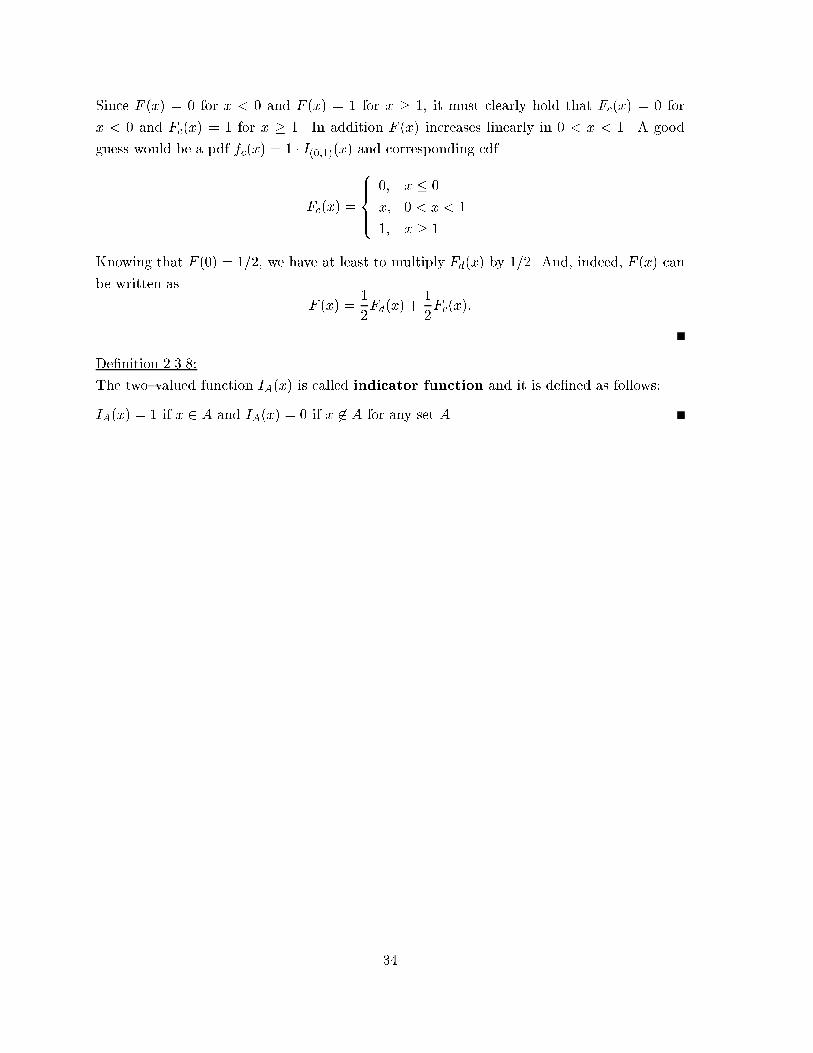
Since F (x) = 0 for x < 0 and F (x) = 1 for x � 1, it must clearly hold that Fc(x) = 0 for

x < 0 and Fc(x) = 1 for x � 1. In addition F (x) increases linearly in 0 < x < 1. A good

guess would be a pdf fc(x) = 1 � I(0;1)(x) and corresponding cdf

Fc(x) =

8>><>>:

0; x � 0

x; 0 < x < 1

1; x � 1

Knowing that F (0) = 1=2, we have at least to multiply Fd(x) by 1=2. And, indeed, F (x) can

be written as

F (x) =1

2Fd(x) +

1

2Fc(x):

De�nition 2.3.8:

The two{valued function IA(x) is called indicator function and it is de�ned as follows:

IA(x) = 1 if x 2 A and IA(x) = 0 if x 62 A for any set A.

34

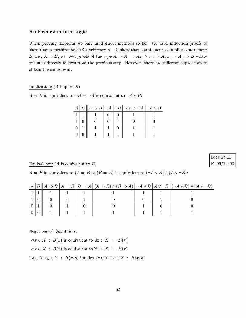
An Excursion into Logic

When proving theorems we only used direct methods so far. We used induction proofs to

show that something holds for arbitrary n. To show that a statement A implies a statement

B, i.e., A ) B, we used proofs of the type A ) A1 ) A2 ) : : : ) An�1 ) An ) B where

one step directly follows from the previous step. However, there are di�erent approaches to

obtain the same result.

Implication: (A implies B)

A) B is equivalent to :B ) :A is equivalent to :A _B:

A B A) B :A :B :B ) :A :A _B1 1 1 0 0 1 1

1 0 0 0 1 0 0

0 1 1 1 0 1 1

0 0 1 1 1 1 1

Lecture 11:

Fr 09/22/00Equivalence: (A is equivalent to B)

A, B is equivalent to (A) B) ^ (B ) A) is equivalent to (:A _B) ^ (A _ :B):

A B A, B A) B B ) A (A) B) ^ (B ) A) :A _B A _ :B (:A _B) ^ (A _ :B)1 1 1 1 1 1 1 1 1

1 0 0 0 1 0 0 1 0

0 1 0 1 0 0 1 0 0

0 0 1 1 1 1 1 1 1

Negations of Quanti�ers:

:8x 2 X : B(x) is equivalent to 9x 2 X : :B(x)

:9x 2 X : B(x) is equivalent to 8x 2 X : :B(x)

9x 2 X 8y 2 Y : B(x; y) implies 8y 2 Y 9x 2 X : B(x; y)

35

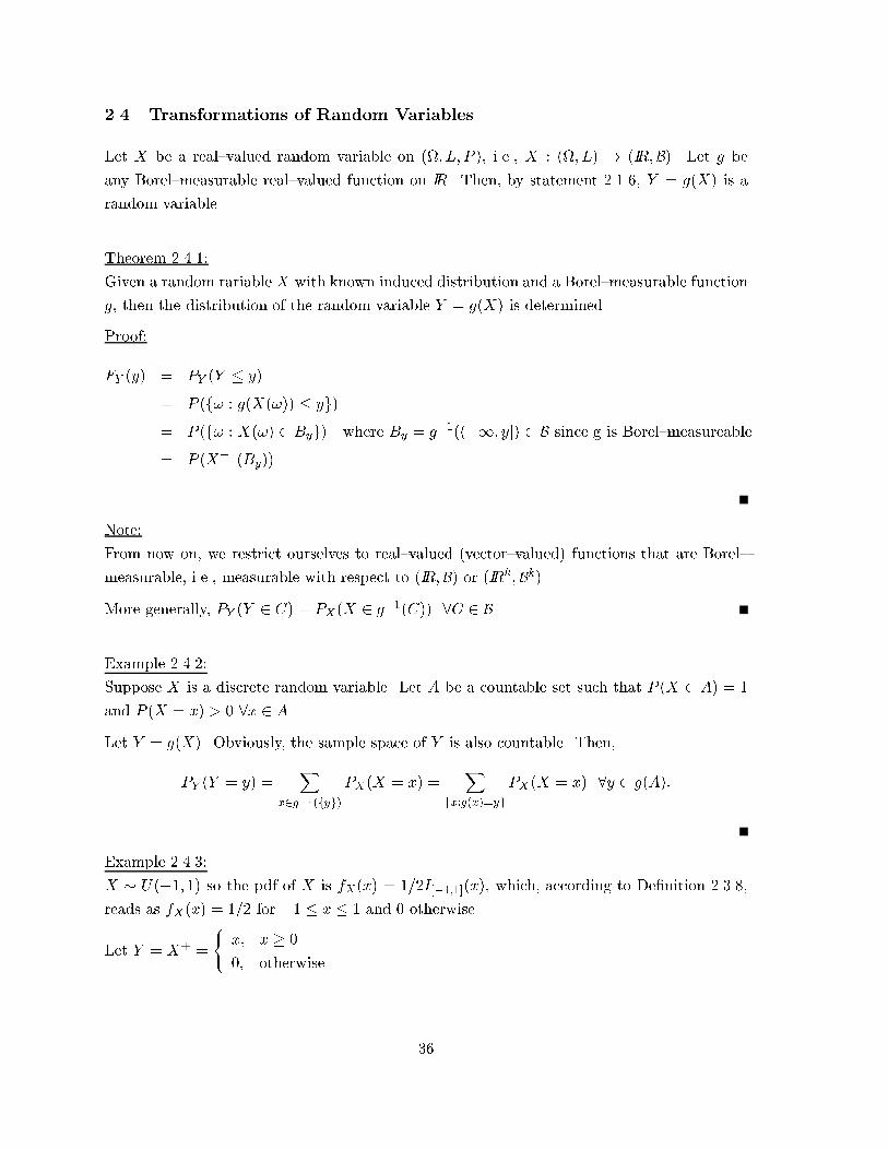
2.4 Transformations of Random Variables

Let X be a real{valued random variable on (; L; P ), i.e., X : (; L) ! (IR;B). Let g be

any Borel{measurable real{valued function on IR. Then, by statement 2.1.6, Y = g(X) is a

random variable.

Theorem 2.4.1:

Given a random rariable X with known induced distribution and a Borel{measurable function

g, then the distribution of the random variable Y = g(X) is determined.

Proof:

FY (y) = PY (Y � y)

= P (f! : g(X(!)) � yg)

= P (f! : X(!) 2 Byg) where By = g�1((�1; y]) 2 B since g is Borel{measureable.

= P (X�1(By))

Note:

From now on, we restrict ourselves to real{valued (vector{valued) functions that are Borel{

measurable, i.e., measurable with respect to (IR;B) or (IRk;Bk).

More generally, PY (Y 2 C) = PX(X 2 g�1(C)) 8C 2 B.

Example 2.4.2:

Suppose X is a discrete random variable. Let A be a countable set such that P (X 2 A) = 1

and P (X = x) > 0 8x 2 A.

Let Y = g(X). Obviously, the sample space of Y is also countable. Then,

PY (Y = y) =X

x2g�1(fyg)PX(X = x) =

Xfx:g(x)=yg

PX(X = x) 8y 2 g(A):

Example 2.4.3:

X � U(�1; 1) so the pdf of X is fX(x) = 1=2I[�1;1](x), which, according to De�nition 2.3.8,

reads as fX(x) = 1=2 for �1 � x � 1 and 0 otherwise.

Let Y = X+ =

(x; x � 0

0; otherwise

36

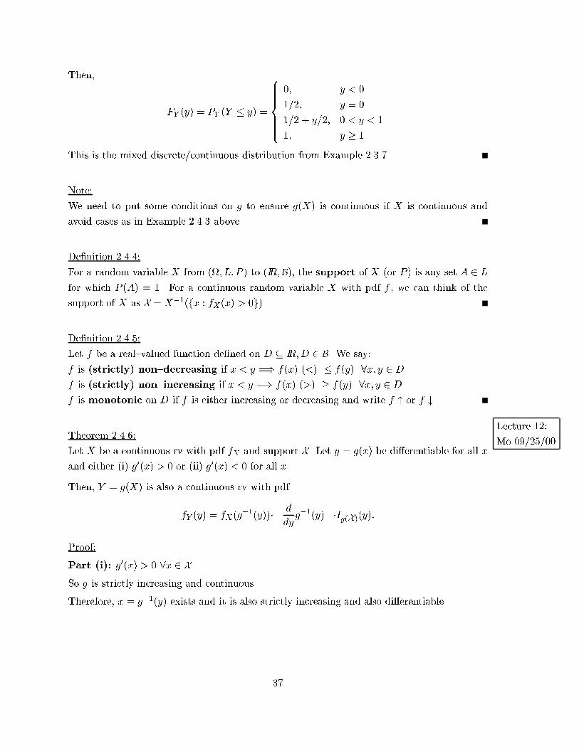
Then,

FY (y) = PY (Y � y) =

8>>>>><>>>>>:

0; y < 0

1=2; y = 0

1=2 + y=2; 0 < y < 1

1; y � 1

This is the mixed discrete/continuous distribution from Example 2.3.7.

Note:

We need to put some conditions on g to ensure g(X) is continuous if X is continuous and

avoid cases as in Example 2.4.3 above.

De�nition 2.4.4:

For a random variable X from (; L; P ) to (IR;B), the support of X (or P ) is any set A 2 L

for which P (A) = 1. For a continuous random variable X with pdf f , we can think of the

support of X as X = X�1(fx : fX(x) > 0g).

De�nition 2.4.5:

Let f be a real{valued function de�ned on D � IR;D 2 B. We say:

f is (strictly) non{decreasing if x < y =) f(x) (<) � f(y) 8x; y 2 D

f is (strictly) non{increasing if x < y =) f(x) (>) � f(y) 8x; y 2 D

f is monotonic on D if f is either increasing or decreasing and write f " or f #.

Lecture 12:

Mo 09/25/00Theorem 2.4.6:

Let X be a continuous rv with pdf fX and support X. Let y = g(x) be di�erentiable for all x

and either (i) g0(x) > 0 or (ii) g0(x) < 0 for all x.

Then, Y = g(X) is also a continuous rv with pdf

fY (y) = fX(g�1(y))� j d

dyg�1(y) j �Ig(X)(y):

Proof:

Part (i): g0(x) > 0 8x 2 X

So g is strictly increasing and continuous.

Therefore, x = g�1(y) exists and it is also strictly increasing and also di�erentiable.

37

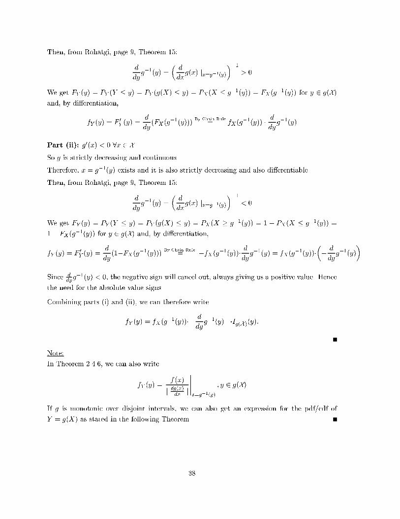
Then, from Rohatgi, page 9, Theorem 15:

d

dyg�1(y) =

�d

dxg(x) jx=g�1(y)

��1> 0

We get FY (y) = PY (Y � y) = PY (g(X) � y) = PX(X � g�1(y)) = FX(g

�1(y)) for y 2 g(X)

and, by di�erentiation,

fY (y) = F0Y (y) =

d

dy(FX(g

�1(y)))By Chain Rule

= fX(g�1(y)) � d

dyg�1(y)

Part (ii): g0(x) < 0 8x 2 X

So g is strictly decreasing and continuous.

Therefore, x = g�1(y) exists and it is also strictly decreasing and also di�erentiable.

Then, from Rohatgi, page 9, Theorem 15:

d

dyg�1(y) =

�d

dxg(x) jx=g�1(y)

��1< 0

We get FY (y) = PY (Y � y) = PY (g(X) � y) = PX(X � g�1(y)) = 1 � PX(X � g

�1(y)) =

1� FX(g�1(y)) for y 2 g(X) and, by di�erentiation,

fY (y) = F0Y (y) =

d

dy(1�FX(g�1(y)))

By Chain Rule= �fX(g�1(y))�

d

dyg�1(y) = fX(g

�1(y))��� d

dyg�1(y)

�

Since ddy g

�1(y) < 0, the negative sign will cancel out, always giving us a positive value. Hence

the need for the absolute value signs.

Combining parts (i) and (ii), we can therefore write

fY (y) = fX(g�1(y))� j d

dyg�1(y) j �Ig(X)(y):

Note:

In Theorem 2.4.6, we can also write

fY (y) =f(x)

j dg(x)dx j

�����x=g�1(y)

; y 2 g(X)

If g is monotonic over disjoint intervals, we can also get an expression for the pdf/cdf of

Y = g(X) as stated in the following Theorem.

38

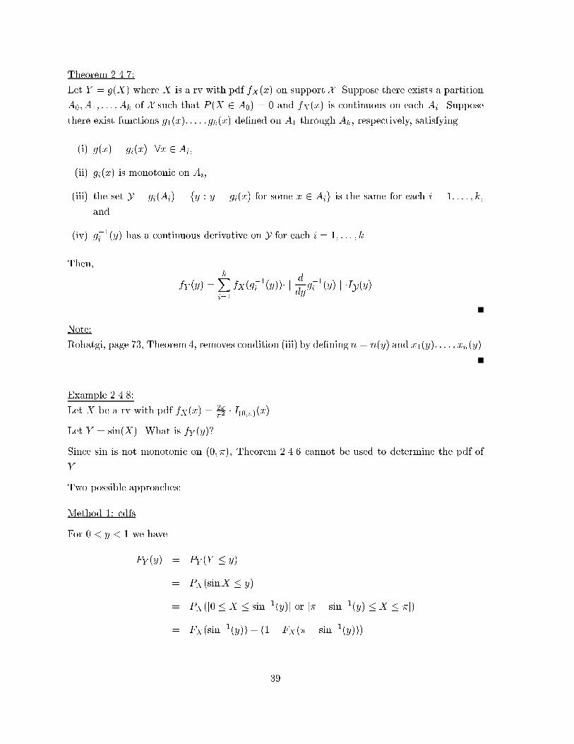
Theorem 2.4.7:

Let Y = g(X) where X is a rv with pdf fX(x) on support X. Suppose there exists a partition

A0; A1; : : : ; Ak of X such that P (X 2 A0) = 0 and fX(x) is continuous on each Ai. Suppose

there exist functions g1(x); : : : ; gk(x) de�ned on A1 through Ak, respectively, satisfying

(i) g(x) = gi(x) 8x 2 Ai,

(ii) gi(x) is monotonic on Ai,

(iii) the set Y = gi(Ai) = fy : y = gi(x) for some x 2 Aig is the same for each i = 1; : : : ; k,

and

(iv) g�1i (y) has a continuous derivative on Y for each i = 1; : : : ; k.

Then,

fY (y) =kXi=1

fX(g�1i (y))� j d

dyg�1i (y) j �IY(y)

Note:

Rohatgi, page 73, Theorem 4, removes condition (iii) by de�ning n = n(y) and x1(y); : : : ; xn(y).

Example 2.4.8:

Let X be a rv with pdf fX(x) =2x�2� I(0;�)(x).

Let Y = sin(X). What is fY (y)?

Since sin is not monotonic on (0; �), Theorem 2.4.6 cannot be used to determine the pdf of

Y .

Two possible approaches:

Method 1: cdfs

For 0 < y < 1 we have

FY (y) = PY (Y � y)

= PX(sinX � y)

= PX([0 � X � sin�1(y)] or [� � sin�1(y) � X � �])

= FX(sin�1(y)) + (1� FX(� � sin�1(y)))

39

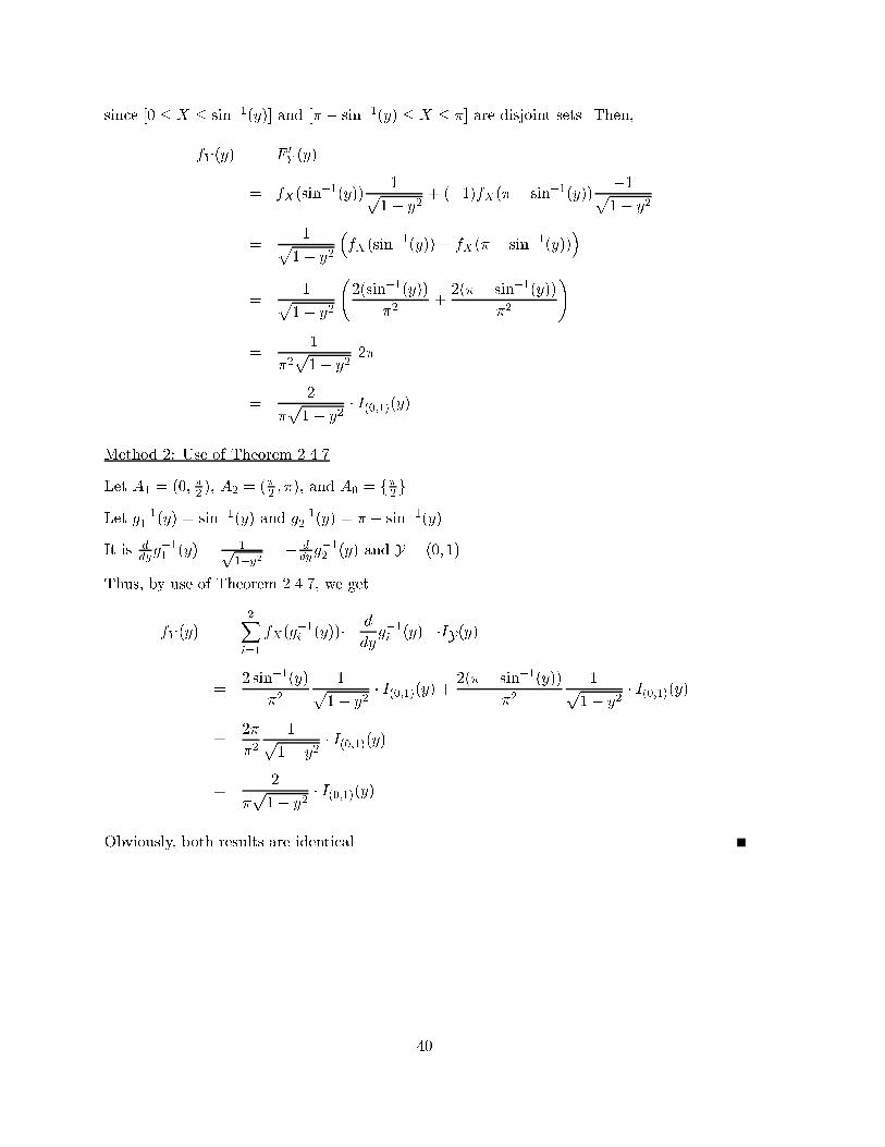
since [0 � X � sin�1(y)] and [� � sin�1(y) � X � �] are disjoint sets. Then,

fY (y) = F0Y (y)

= fX(sin�1(y))

1p1� y2

+ (�1)fX(� � sin�1(y))�1p1� y2

=1p

1� y2

�fX(sin

�1(y)) + fX(� � sin�1(y))�

=1p

1� y2

2(sin�1(y))

�2+2(� � sin�1(y))

�2

!

=1

�2p1� y2

2�

=2

�p1� y2

� I(0;1)(y)

Method 2: Use of Theorem 2.4.7

Let A1 = (0; �2 ), A2 = (�2 ; �), and A0 = f�2 g.

Let g�11 (y) = sin�1(y) and g�12 (y) = � � sin�1(y).

It is ddyg�11 (y) = 1p

1�y2= � d

dyg�12 (y) and Y = (0; 1).

Thus, by use of Theorem 2.4.7, we get

fY (y) =2Xi=1

fX(g�1i (y))� j d

dyg�1i (y) j �IY(y)

=2 sin�1(y)

�2

1p1� y2

� I(0;1)(y) +2(� � sin�1(y))

�2

1p1� y2

� I(0;1)(y)

=2�

�2

1p1� y2

� I(0;1)(y)

=2

�p1� y2

� I(0;1)(y)

Obviously, both results are identical.

40

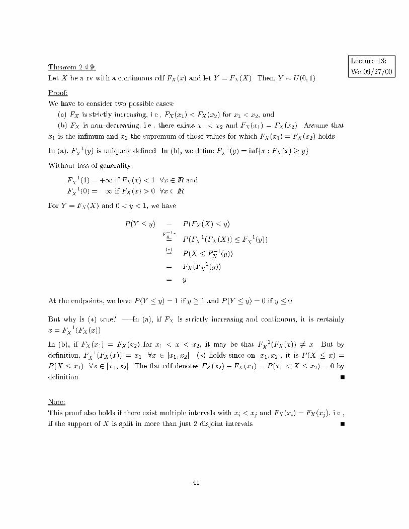
Lecture 13:

We 09/27/00Theorem 2.4.9:

Let X be a rv with a continuous cdf FX(x) and let Y = FX(X). Then, Y � U(0; 1).

Proof:

We have to consider two possible cases:

(a) FX is strictly increasing, i.e., FX(x1) < FX(x2) for x1 < x2, and

(b) FX is non{decreasing, i.e., there exists x1 < x2 and FX(x1) = FX(x2). Assume that

x1 is the in�mum and x2 the supremum of those values for which FX(x1) = FX(x2) holds.

In (a), F�1X (y) is uniquely de�ned. In (b), we de�ne F�1

X (y) = inffx : FX(x) � yg

Without loss of generality:

F�1X (1) = +1 if FX(x) < 1 8x 2 IR and

F�1X (0) = �1 if FX(x) > 0 8x 2 IR.

For Y = FX(X) and 0 < y < 1, we have

P (Y � y) = P (FX(X) � y)

F�1X

"= P (F�1

X (FX(X)) � F�1X (y))

(�)= P (X � F

�1X (y))

= FX(F�1X (y))

= y

At the endpoints, we have P (Y � y) = 1 if y � 1 and P (Y � y) = 0 if y � 0.

But why is (�) true? | In (a), if FX is strictly increasing and continuous, it is certainly

x = F�1X (FX(x)).

In (b), if FX(x1) = FX(x2) for x1 < x < x2, it may be that F�1X (FX(x)) 6= x. But by

de�nition, F�1X (FX(x)) = x1 8x 2 [x1; x2]. (�) holds since on [x1; x2], it is P (X � x) =

P (X � x1) 8x 2 [x1; x2]. The at cdf denotes FX(x2) � FX(x1) = P (x1 < X � x2) = 0 by

de�nition.

Note:

This proof also holds if there exist multiple intervals with xi < xj and FX(xi) = FX(xj), i.e.,

if the support of X is split in more than just 2 disjoint intervals.

41

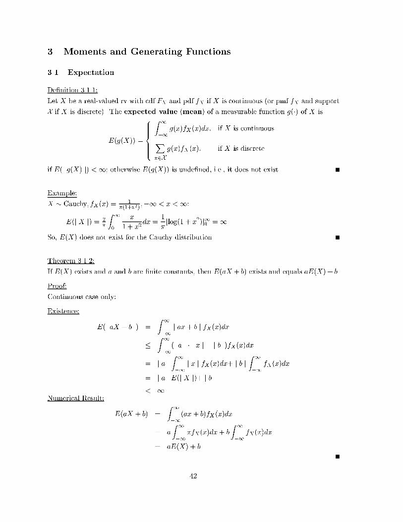
3 Moments and Generating Functions

3.1 Expectation

De�nition 3.1.1:

Let X be a real-valued rv with cdf FX and pdf fX if X is continuous (or pmf fX and support

X if X is discrete). The expected value (mean) of a measurable function g(�) of X is

E(g(X)) =

8>>>><>>>>:

Z 1

�1g(x)fX(x)dx; if X is continuous

Xx2X

g(x)fX(x); if X is discrete

if E(j g(X) j) <1; otherwise E(g(X)) is unde�ned, i.e., it does not exist.

Example:

X � Cauchy; fX(x) =1

�(1+x2);�1 < x <1:

E(j X j) = 2�

Z 1

0

x

1 + x2dx =

1

�[log(1 + x

2)]10 =1

So, E(X) does not exist for the Cauchy distribution.

Theorem 3.1.2:

If E(X) exists and a and b are �nite constants, then E(aX + b) exists and equals aE(X) + b.

Proof:

Continuous case only:

Existence:

E(j aX + b j) =

Z 1

�1j ax+ b j fX(x)dx

�Z 1

�1(j a j � j x j + j b j)fX(x)dx

= j a jZ 1

�1j x j fX(x)dx+ j b j

Z 1

�1fX(x)dx

= j a j E(j X j)+ j b j

< 1Numerical Result:

E(aX + b) =

Z 1

�1(ax+ b)fX(x)dx

= a

Z 1

�1xfX(x)dx+ b

Z 1

�1fX(x)dx

= aE(X) + b

42

Lecture 14:

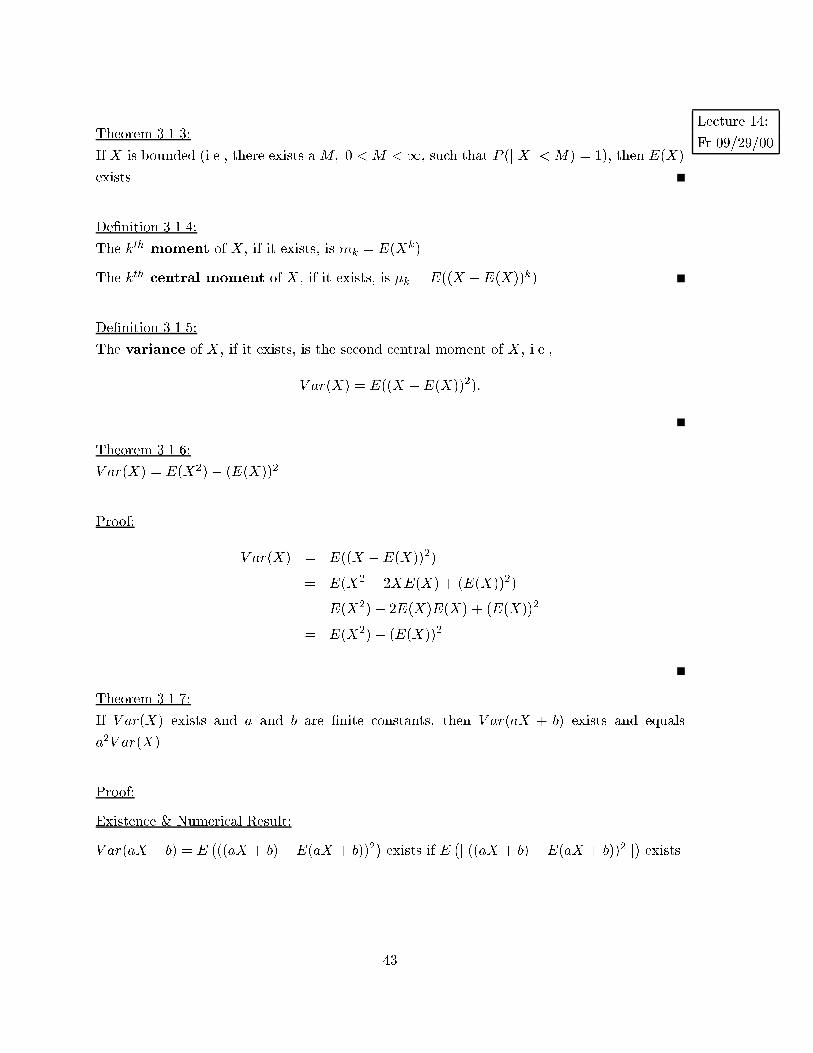
Fr 09/29/00Theorem 3.1.3:

If X is bounded (i.e., there exists a M; 0 < M <1, such that P (j X j< M) = 1), then E(X)

exists.

De�nition 3.1.4:

The kth moment of X, if it exists, is mk = E(Xk).

The kth central moment of X, if it exists, is �k = E((X �E(X))k).

De�nition 3.1.5:

The variance of X, if it exists, is the second central moment of X, i.e.,

V ar(X) = E((X �E(X))2):

Theorem 3.1.6:

V ar(X) = E(X2)� (E(X))2.

Proof:

V ar(X) = E((X �E(X))2)

= E(X2 � 2XE(X) + (E(X))2)

= E(X2)� 2E(X)E(X) + (E(X))2

= E(X2)� (E(X))2

Theorem 3.1.7:

If V ar(X) exists and a and b are �nite constants, then V ar(aX + b) exists and equals

a2V ar(X).

Proof:

Existence & Numerical Result:

V ar(aX + b) = E�((aX + b)�E(aX + b))2

�exists if E

�j ((aX + b)�E(aX + b))2 j

�exists.

43

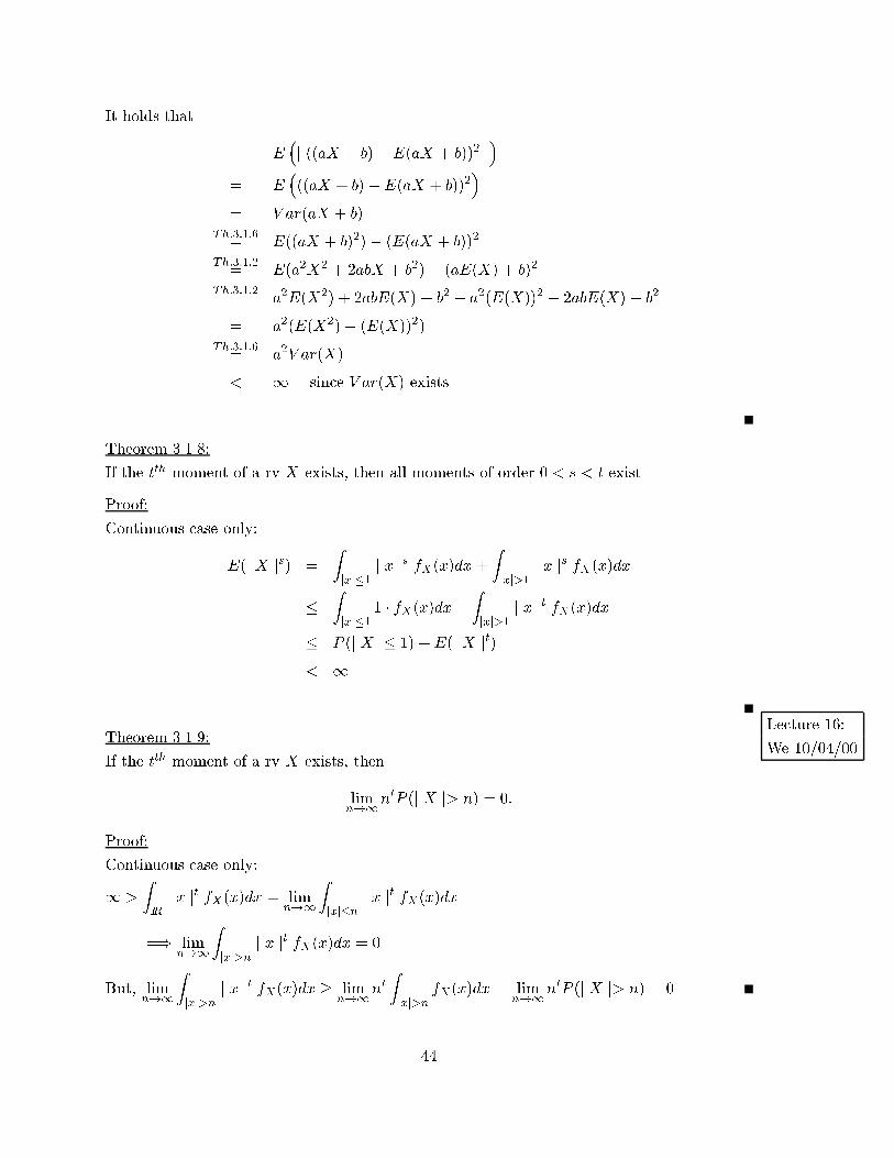
It holds that

E

�j ((aX + b)�E(aX + b))2 j

�= E

�((aX + b)�E(aX + b))2

�= V ar(aX + b)

Th:3:1:6= E((aX + b)2)� (E(aX + b))2

Th:3:1:2= E(a2X2 + 2abX + b

2)� (aE(X) + b)2

Th:3:1:2= a

2E(X2) + 2abE(X) + b

2 � a2(E(X))2 � 2abE(X) � b

2

= a2(E(X2)� (E(X))2)

Th:3:1:6= a

2V ar(X)

< 1 since V ar(X) exists

Theorem 3.1.8:

If the tth moment of a rv X exists, then all moments of order 0 < s < t exist.

Proof:

Continuous case only:

E(j X js) =

Zjxj�1

j x js fX(x)dx+Zjxj>1

j x js fX(x)dx

�Zjxj�1

1 � fX(x)dx+Zjxj>1

j x jt fX(x)dx

� P (j X j� 1) +E(j X jt)

< 1

Lecture 16:

We 10/04/00Theorem 3.1.9:

If the tth moment of a rv X exists, then

limn!1n

tP (j X j> n) = 0:

Proof:

Continuous case only:

1 >

ZIRj x jt fX(x)dx = lim

n!1

Zjxj�n

j x jt fX(x)dx

=) limn!1

Zjxj>n

j x jt fX(x)dx = 0

But, limn!1

Zjxj>n

j x jt fX(x)dx � limn!1n

tZjxj>n

fX(x)dx = limn!1n

tP (j X j> n) = 0

44

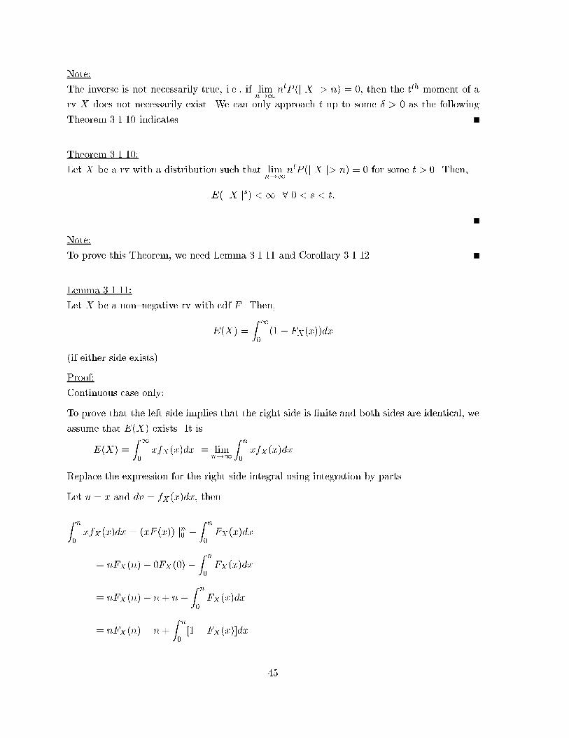
Note:

The inverse is not necessarily true, i.e., if limn!1n

tP (j X j> n) = 0, then the tth moment of a

rv X does not necessarily exist. We can only approach t up to some � > 0 as the following

Theorem 3.1.10 indicates.

Theorem 3.1.10:

Let X be a rv with a distribution such that limn!1n

tP (j X j> n) = 0 for some t > 0. Then,

E(j X js) <1 8 0 < s < t:

Note:

To prove this Theorem, we need Lemma 3.1.11 and Corollary 3.1.12.

Lemma 3.1.11:

Let X be a non{negative rv with cdf F . Then,

E(X) =

Z 1

0(1� FX(x))dx

(if either side exists).

Proof:

Continuous case only:

To prove that the left side implies that the right side is �nite and both sides are identical, we

assume that E(X) exists. It is

E(X) =

Z 1

0xfX(x)dx = lim

n!1

Z n

0xfX(x)dx

Replace the expression for the right side integral using integration by parts.

Let u = x and dv = fX(x)dx, then

Z n

0xfX(x)dx = (xF (x)) jn0 �

Z n

0FX(x)dx

= nFX(n)� 0FX (0)�Z n

0FX(x)dx

= nFX(n)� n+ n�Z n

0FX(x)dx

= nFX(n)� n+

Z n

0[1� FX(x)]dx

45

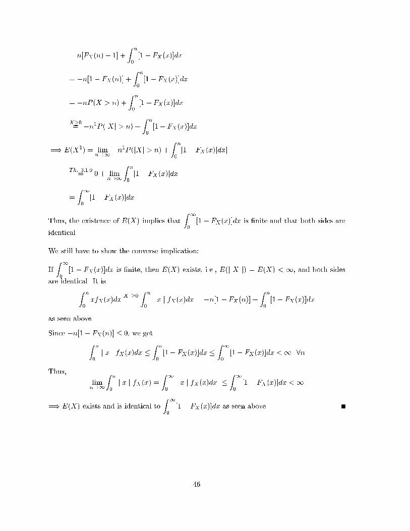
= n[FX(n)� 1] +

Z n

0[1� FX(x)]dx

= �n[1� FX(n)] +

Z n

0[1� FX(x)]dx

= �nP (X > n) +

Z n

0[1� FX(x)]dx

X�0= �n1P (jXj > n) +

Z n

0[1� FX(x)]dx

=) E(X1) = limn!1[�n

1P (jXj > n) +

Z n

0[1� FX(x)]dx]

Th: 3:1:9= 0 + lim

n!1

Z n

0[1� FX(x)]dx

=

Z 1

0[1� FX(x)]dx

Thus, the existence of E(X) implies that

Z 1

0[1 � FX(x)]dx is �nite and that both sides are

identical.

We still have to show the converse implication:

If

Z 1

0[1 � FX(x)]dx is �nite, then E(X) exists, i.e., E(j X j) = E(X) < 1, and both sides

are identical. It isZ n

0xfX(x)dx

X �0=

Z n

0j x j fX(x)dx = �n[1� FX(n)] +

Z n

0[1� FX(x)]dx

as seen above.

Since �n[1� FX(n)] � 0, we get

Z n

0j x j fX(x)dx �

Z n

0[1� FX(x)]dx �

Z 1

0[1� FX(x)]dx <1 8n

Thus,

limn!1

Z n

0j x j fX(x) =

Z 1

0j x j fX(x)dx �

Z 1

0[1� FX(x)]dx <1

=) E(X) exists and is identical to

Z 1

0[1� FX(x)]dx as seen above.

46

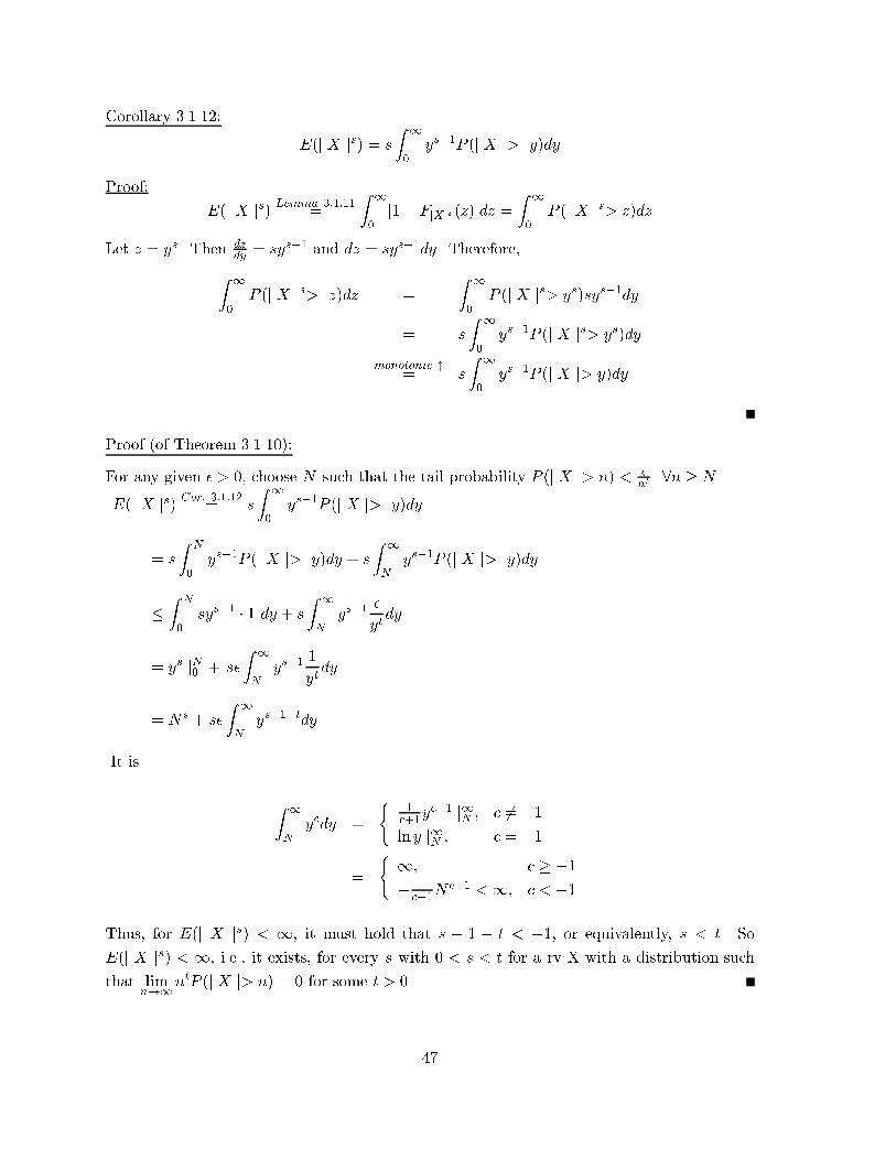
Corollary 3.1.12:

E(j X js) = s

Z 1

0ys�1

P (j X j> y)dy

Proof:

E(j X js) Lemma 3:1:11=

Z 1

0[1� FjXjs(z)]dz =

Z 1

0P (j X js> z)dz

Let z = ys. Then dz

dy = sys�1 and dz = sy

s�1dy. Therefore,

Z 1

0P (j X js> z)dz =

Z 1

0P (j X js> y

s)sys�1dy

= s

Z 1

0ys�1

P (j X js> ys)dy

monotonic "= s

Z 1

0ys�1

P (j X j> y)dy

Proof (of Theorem 3.1.10):

For any given � > 0, choose N such that the tail probability P (j X j> n) < �nt

8n � N .

E(j X js) Cor: 3:1:12= s

Z 1

0ys�1

P (j X j> y)dy

= s

Z N

0ys�1

P (j X j> y)dy + s

Z 1

Nys�1

P (j X j> y)dy

�Z N

0sy

s�1 � 1 dy + s

Z 1

Nys�1 �

ytdy

= ys jN0 + s�

Z 1

Nys�1 1

ytdy

= Ns + s�

Z 1

Nys�1�t

dy

It is

Z 1

Nycdy =

(1

c+1yc+1 j1N ; c 6= �1

ln y j1N ; c = �1

=

(1; c � �1� 1

c+1Nc+1

<1; c < �1

Thus, for E(j X js) < 1, it must hold that s � 1 � t < �1, or equivalently, s < t. So

E(j X js) < 1, i.e., it exists, for every s with 0 < s < t for a rv X with a distribution such

that limn!1n

tP (j X j> n) = 0 for some t > 0.

47

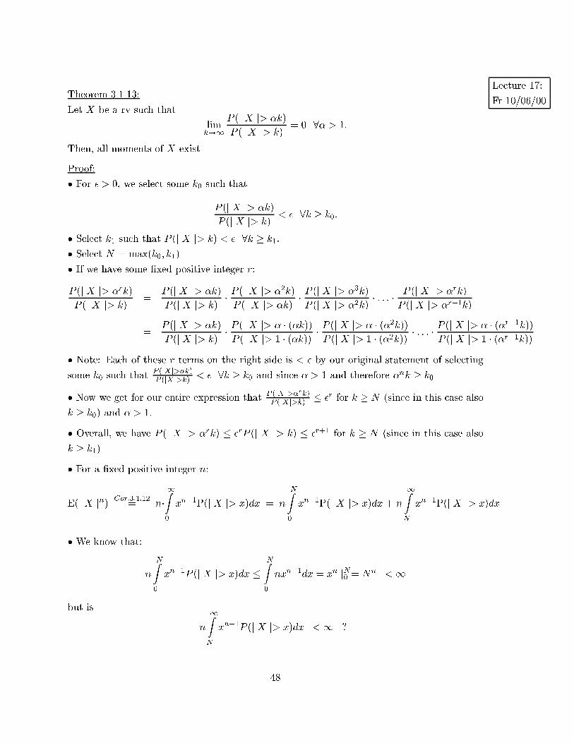
Lecture 17:

Fr 10/06/00Theorem 3.1.13:

Let X be a rv such that

limk!1

P (j X j> �k)

P (j X j> k)= 0 8� > 1:

Then, all moments of X exist.

Proof:

� For � > 0; we select some k0 such that

P (j X j> �k)

P (j X j> k)< � 8k � k0:

� Select k1 such that P (j X j> k) < � 8k � k1:

� Select N = max(k0; k1).

� If we have some �xed positive integer r:

P (j X j> �rk)

P (j X j> k)=

P (j X j> �k)

P (j X j> k)� P (j X j> �

2k)

P (j X j> �k)� P (j X j> �

3k)

P (j X j> �2k)� : : : � P (j X j> �

rk)

P (j X j> �r�1k)

=P (j X j> �k)

P (j X j> k)� P (j X j> � � (�k))P (j X j> 1 � (�k)) �

P (j X j> � � (�2k))P (j X j> 1 � (�2k)) � : : : �

P (j X j> � � (�r�1k))P (j X j> 1 � (�r�1k))

� Note: Each of these r terms on the right side is < � by our original statement of selecting

some k0 such thatP (jXj>�k)P (jXj>k) < � 8k � k0 and since � > 1 and therefore �nk � k0.

� Now we get for our entire expression thatP (jXj>�rk)P (jXj>k) � �

r for k � N (since in this case also

k � k0) and � > 1:

� Overall, we have P (j X j> �rk) � �

rP (j X j> k) � �

r+1 for k � N (since in this case also

k � k1).

� For a �xed positive integer n:

E(j X jn) Cor:3:1:12= n�

1Z0

xn�1P(j X j> x)dx = n

NZ0

xn�1P(j X j> x)dx + n

1ZN

xn�1P(j X j> x)dx

� We know that:

n

NZ0

xn�1

P (j X j> x)dx �NZ0

nxn�1

dx = xn jN0 = N

n<1

but is

n

1ZN

xn�1

P (j X j> x)dx <1 ?

48

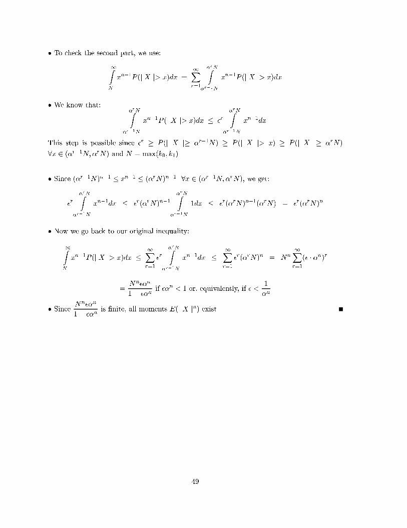
� To check the second part, we use:

1ZN

xn�1

P (j X j> x)dx =1Xr=1

�rNZ�r�1N

xn�1

P (j X j> x)dx

� We know that:�rNZ

�r�1N

xn�1

P (j X j> x)dx � �r

�rNZ�r�1N

xn�1

dx

This step is possible since �r � P (j X j� �

r�1N) � P (j X j> x) � P (j X j� �

rN)

8x 2 (�r�1N;�rN) and N = max(k0; k1).

� Since (�r�1N)n�1 � xn�1 � (�rN)n�1 8x 2 (�r�1N;�rN), we get:

�r

�rNZ�r�1N

xn�1

dx � �r(�rN)n�1

�rNZ�r�1N

1dx � �r(�rN)n�1(�rN) = �

r(�rN)n

� Now we go back to our original inequality:

1ZN

xn�1

P (j X j> x)dx �1Xr=1

�r

�rNZ�r�1N

xn�1

dx �1Xr=1

�r(�rN)n = N

n1Xr=1

(� � �n)r

=N

n��

n

1� ��nif ��n < 1 or, equivalently, if � <

1

�n

� Since Nn��

n

1� ��nis �nite, all moments E(j X jn) exist.

49

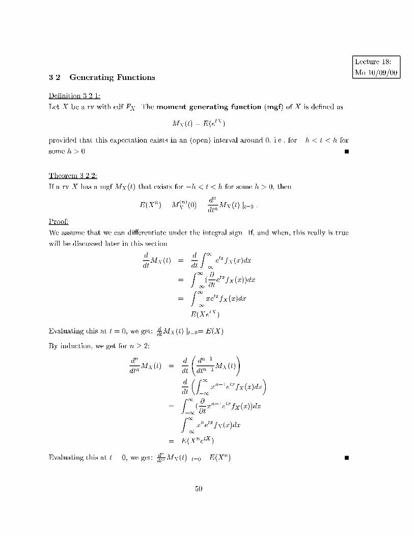
Lecture 18:

Mo 10/09/003.2 Generating Functions

De�nition 3.2.1:

Let X be a rv with cdf FX . The moment generating function (mgf) of X is de�ned as

MX(t) = E(etX )

provided that this expectation exists in an (open) interval around 0, i.e., for �h < t < h for

some h > 0.

Theorem 3.2.2:

If a rv X has a mgf MX(t) that exists for �h < t < h for some h > 0, then

E(Xn) =M(n)X (0) =

dn

dtnMX(t) jt=0 :

Proof:

We assume that we can di�erentiate under the integral sign. If, and when, this really is true

will be discussed later in this section.

d

dtMX(t) =

d

dt

Z 1

�1etxfX(x)dx

=

Z 1

�1(@

@tetxfX(x))dx

=

Z 1

�1xe

txfX(x)dx

= E(XetX )

Evaluating this at t = 0, we get: ddtMX(t) jt=0= E(X)

By induction, we get for n � 2:

dn

dtnMX(t) =

d

dt

dn�1

dtn�1MX(t)

!

=d

dt

�Z 1

�1xn�1

etxfX(x)dx

�

=

Z 1

�1(@

@txn�1

etxfX(x))dx

=

Z 1

�1xnetxfX(x)dx

= E(XnetX)

Evaluating this at t = 0, we get: dn

dtnMX(t) jt=0= E(Xn)

50

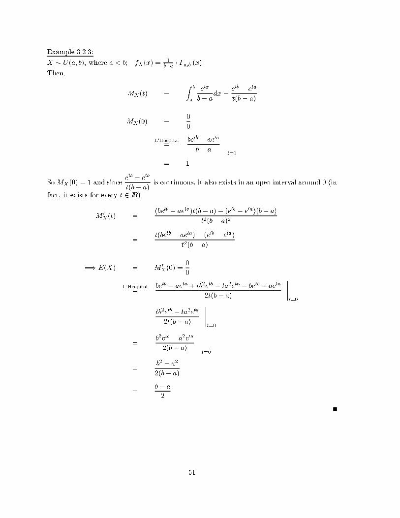
Example 3.2.3:

X � U(a; b), where a < b; fX(x) =1

b�a � I[a;b](x).Then,

MX(t) =

Z b

a

etx

b� adx =

etb � e

ta

t(b� a)

MX(0) =0

0

L'Hospital=

betb � ae

ta

b� a

�����t=0

= 1

So MX(0) = 1 and sinceetb � e

ta

t(b� a)is continuous, it also exists in an open interval around 0 (in

fact, it exists for every t 2 IR).

M0X(t) =

(betb � aeta)t(b� a)� (etb � e

ta)(b� a)

t2(b� a)2

=t(betb � ae

ta)� (etb � eta)

t2(b� a)

=) E(X) = M0X(0) =

0

0

L'Hospital=

betb � ae

ta + tb2etb � ta

2eta � be

tb + aeta

2t(b� a)

�����t=0

=tb2etb � ta

2eta

2t(b� a)

�����t=0

=b2etb � a

2eta

2(b� a)

�����t=0

=b2 � a

2

2(b� a)

=b+ a

2

51

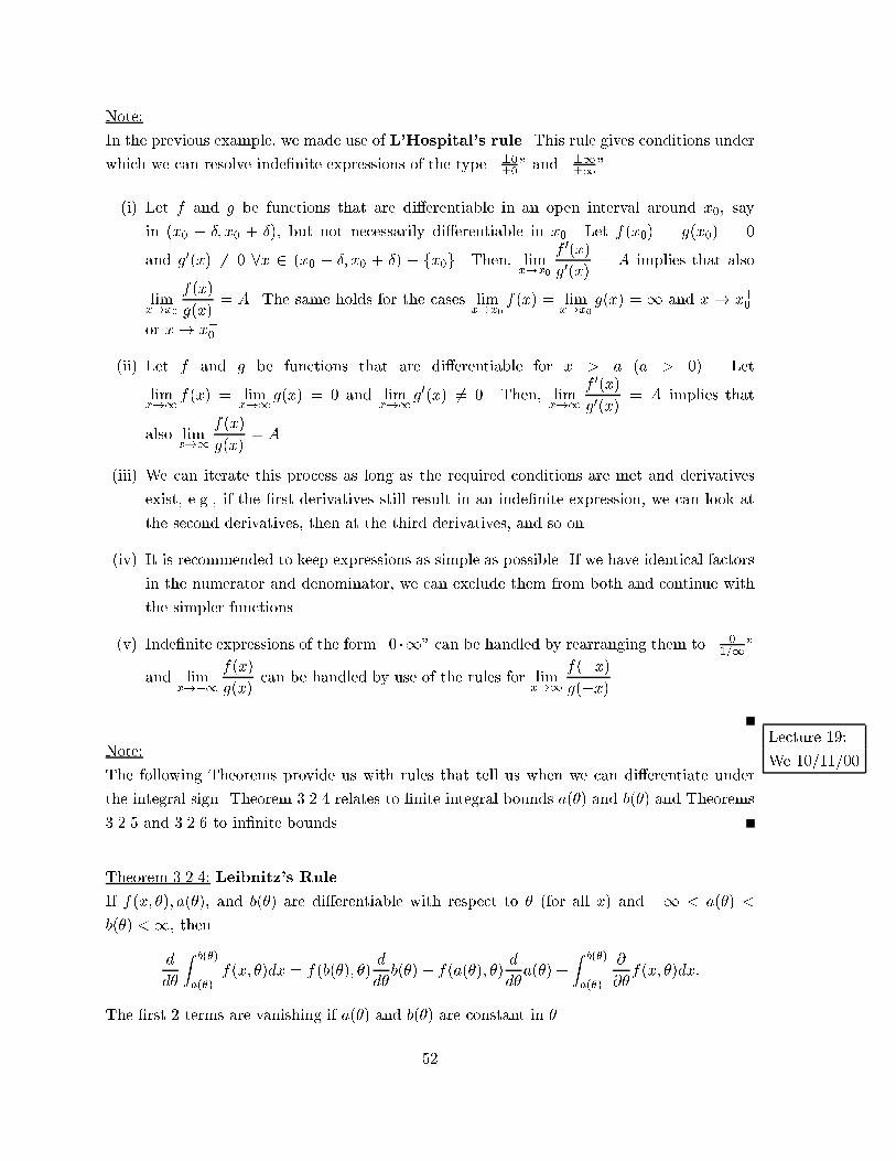
Note:

In the previous example, we made use of L'Hospital's rule. This rule gives conditions under

which we can resolve inde�nite expressions of the type \�0�0" and \�1�1".

(i) Let f and g be functions that are di�erentiable in an open interval around x0, say

in (x0 � �; x0 + �); but not necessarily di�erentiable in x0. Let f(x0) = g(x0) = 0

and g0(x) 6= 0 8x 2 (x0 � �; x0 + �) � fx0g. Then, lim

x!x0

f0(x)g0(x)

= A implies that also

limx!x0

f(x)

g(x)= A. The same holds for the cases lim

x!x0f(x) = lim

x!x0g(x) = 1 and x ! x

+0

or x! x�0 .

(ii) Let f and g be functions that are di�erentiable for x > a (a > 0). Let

limx!1 f(x) = lim

x!1 g(x) = 0 and limx!1 g

0(x) 6= 0. Then, limx!1

f0(x)g0(x)

= A implies that

also limx!1

f(x)

g(x)= A.

(iii) We can iterate this process as long as the required conditions are met and derivatives

exist, e.g., if the �rst derivatives still result in an inde�nite expression, we can look at

the second derivatives, then at the third derivatives, and so on.

(iv) It is recommended to keep expressions as simple as possible. If we have identical factors

in the numerator and denominator, we can exclude them from both and continue with

the simpler functions.

(v) Inde�nite expressions of the form \0 �1" can be handled by rearranging them to \ 01=1"

and limx!�1

f(x)

g(x)can be handled by use of the rules for lim

x!1f(�x)g(�x) .

Lecture 19:

We 10/11/00Note:

The following Theorems provide us with rules that tell us when we can di�erentiate under

the integral sign. Theorem 3.2.4 relates to �nite integral bounds a(�) and b(�) and Theorems

3.2.5 and 3.2.6 to in�nite bounds.

Theorem 3.2.4: Leibnitz's Rule

If f(x; �); a(�), and b(�) are di�erentiable with respect to � (for all x) and �1 < a(�) <

b(�) <1, then

d

d�

Z b(�)

a(�)f(x; �)dx = f(b(�); �)

d

d�b(�)� f(a(�); �)

d

d�a(�) +

Z b(�)

a(�)

@

@�f(x; �)dx:

The �rst 2 terms are vanishing if a(�) and b(�) are constant in �.

52

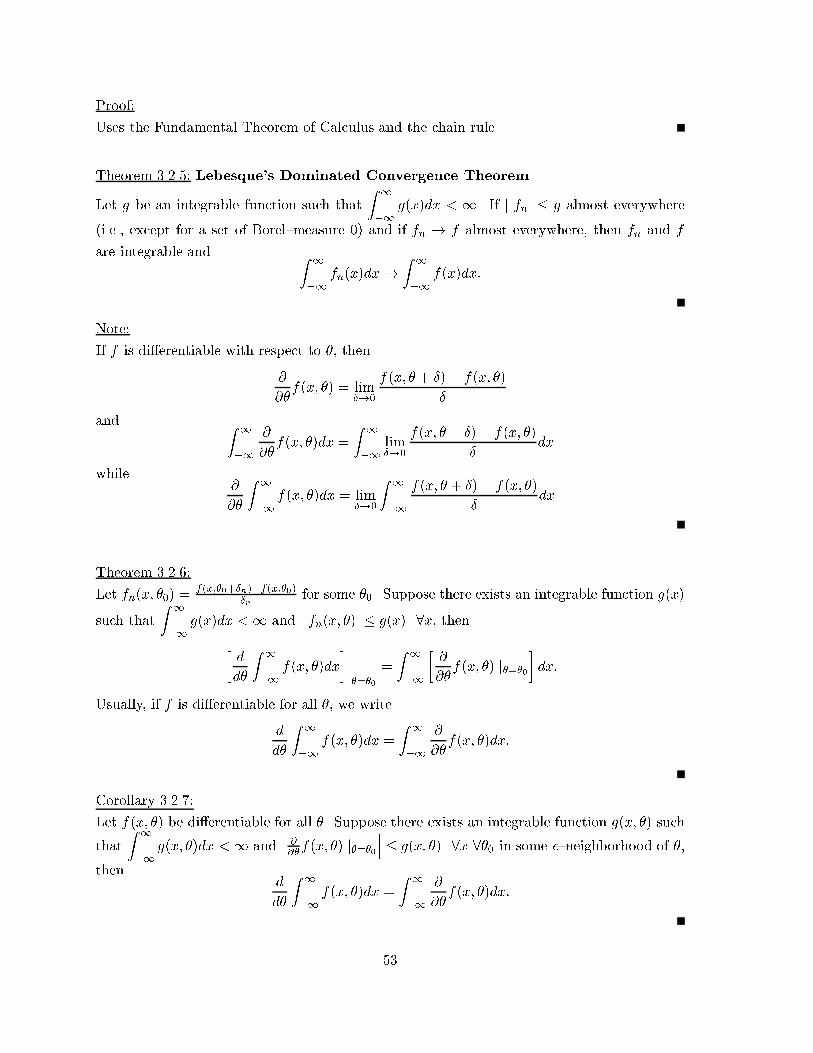
Proof:

Uses the Fundamental Theorem of Calculus and the chain rule.

Theorem 3.2.5: Lebesque's Dominated Convergence Theorem

Let g be an integrable function such that

Z 1

�1g(x)dx < 1. If j fn j� g almost everywhere

(i.e., except for a set of Borel{measure 0) and if fn ! f almost everywhere, then fn and f

are integrable and Z 1

�1fn(x)dx!

Z 1

�1f(x)dx:

Note:

If f is di�erentiable with respect to �, then

@

@�f(x; �) = lim

�!0

f(x; � + �) � f(x; �)

�

and Z 1

�1

@

@�f(x; �)dx =

Z 1

�1lim�!0

f(x; � + �)� f(x; �)

�dx

while@

@�

Z 1

�1f(x; �)dx = lim

�!0

Z 1

�1

f(x; � + �)� f(x; �)

�dx

Theorem 3.2.6:

Let fn(x; �0) =f(x;�0+�n)�f(x;�0)

�nfor some �0. Suppose there exists an integrable function g(x)

such that

Z 1

�1g(x)dx <1 and j fn(x; �) j� g(x) 8x, then

�d

d�

Z 1

�1f(x; �)dx

������=�0

=

Z 1

�1

�@

@�f(x; �) j�=�0

�dx:

Usually, if f is di�erentiable for all �, we write

d

d�

Z 1

�1f(x; �)dx =

Z 1

�1

@

@�f(x; �)dx:

Corollary 3.2.7:

Let f(x; �) be di�erentiable for all �. Suppose there exists an integrable function g(x; �) such

that

Z 1

�1g(x; �)dx <1 and

��� @@�f(x; �) j�=�0��� � g(x; �) 8x 8�0 in some �{neighborhood of �,

thend

d�

Z 1

�1f(x; �)dx =

Z 1

�1

@

@�f(x; �)dx:

53

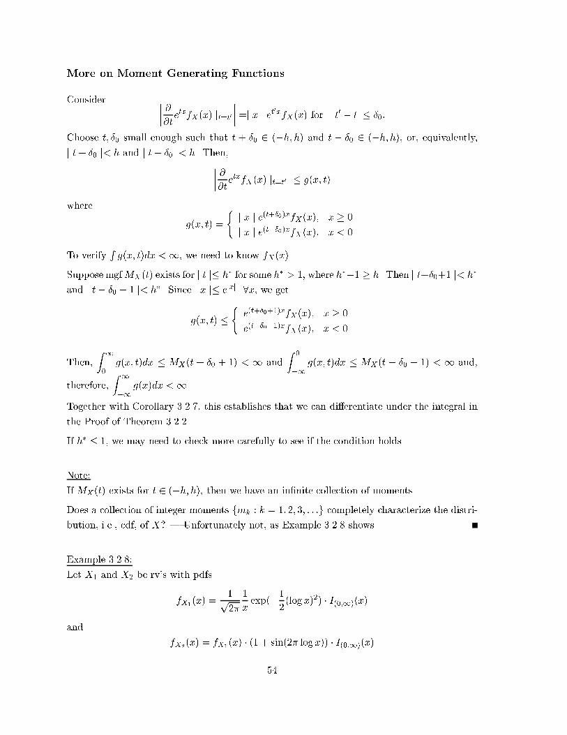
More on Moment Generating Functions

Consider ���� @@tetxfX(x) jt=t0

���� =j x j et0xfX(x) for j t0 � t j� �0:

Choose t; �0 small enough such that t + �0 2 (�h; h) and t � �0 2 (�h; h), or, equivalently,j t+ �0 j< h and j t� �0 j< h. Then,���� @

@tetxfX(x) jt=t0

���� � g(x; t)

where

g(x; t) =

(j x j e(t+�0)xfX(x); x � 0

j x j e(t��0)xfX(x); x < 0

To verifyRg(x; t)dx <1, we need to know fX(x).

Suppose mgfMX(t) exists for j t j� h� for some h� > 1, where h��1 � h. Then j t+�0+1 j< h

�

and j t� �0 � 1 j< h�. Since j x j� e

jxj 8x, we get

g(x; t) �(

e(t+�0+1)xfX(x); x � 0

e(t��0�1)xfX(x); x < 0

Then,

Z 1

0g(x; t)dx � MX(t + �0 + 1) < 1 and

Z 0

�1g(x; t)dx � MX(t � �0 � 1) < 1 and,

therefore,

Z 1

�1g(x)dx <1.

Together with Corollary 3.2.7, this establishes that we can di�erentiate under the integral in

the Proof of Theorem 3.2.2.

If h� � 1, we may need to check more carefully to see if the condition holds.

Note:

If MX(t) exists for t 2 (�h; h), then we have an in�nite collection of moments.

Does a collection of integer moments fmk : k = 1; 2; 3; : : :g completely characterize the distri-bution, i.e., cdf, of X? | Unfortunately not, as Example 3.2.8 shows.

Example 3.2.8:

Let X1 and X2 be rv's with pdfs

fX1(x) =

1p2�

1

xexp(�1

2(log x)2) � I(0;1)(x)

and

fX2(x) = fX1

(x) � (1 + sin(2� log x)) � I(0;1)(x)

54

It is E(Xr1 ) = E(Xr

2 ) = er2=2 for r = 0; 1; 2; : : : as you have to show in the Homeworks.

Two di�erent pdfs/cdfs have the same moment sequence! What went wrong? In this example,

MX1(t) does not exist as shown in the Homeworks!

Lecture 20:

Fr 10/13/00Theorem 3.2.9:

Let X and Y be 2 rv's with cdf's FX and FY for which all moments exist.

(i) If FX and FY have bounded support, then FX(u) = FY (u) 8u i� E(Xr) = E(Y r) for

r = 0; 1; 2; : : :.

(ii) If both mgf's exist, i.e., MX(t) =MY (t) for t in some neighborhood of 0, then FX(u) =

FY (u) 8u.

Note:

The existence of moments is not equivalent to the existence of a mgf as seen in Example 3.2.8

above and some of the Homework assignments.

Theorem 3.2.10:

Suppose rv's fXig1i=1 have mgf'sMXi(t) and that lim

i!1MXi

(t) =MX(t) 8t 2 (�h; h) for someh > 0 and that MX(t) itself is a mgf. Then, there exists a cdf FX whose moments are deter-

mined by MX(t) and for all continuity points x of FX(x) it holds that limi!1

FXi(x) = FX(x),

i.e., the convergence of mgf's implies the convergence of cdf's.

Proof:

Uniqueness of Laplace transformations, etc.

Theorem 3.2.11:

For constants a and b, the mgf of Y = aX + b is

MY (t) = ebtMX(at);

given that MX(t) exists.

Proof:

MY (t) = E(e(aX+b)t)

= E(eaXtebt)

= ebtE(eXat)

= ebtMX(at)

55

3.3 Complex{Valued Random Variables and Characteristic Functions

Recall the following facts regarding complex numbers:

i0 = +1; i =

p�1; i2 = �1; i3 = �i; i4 = +1; etc.

in the planar Gauss'ian number plane it holds that i = (0; 1)

z = a+ ib = r(cos�+ i sin�)

r =j z j=pa2 + b2

tan� = ba

Euler's Relation: z = r(cos�+ i sin�) = rei�

Mathematical Operations on Complex Numbers:

z1 � z2 = (a1 � a2) + i(b1 � b2)

z1 � z2 = r1r2ei(�1+�2) = r1r2(cos(�1 + �2) + i sin(�1 + �2))

z1z2= r1

r2ei(�1��2) = r1

r2(cos(�1 � �2) + i sin(�1 � �2))

Moivre's Theorem: zn = (r(cos�+ i sin�))n = rn(cos(n�) + i sin(n�))

npz = n

pa+ ib = n

pr

�cos(�+k�360

0

n ) + i sin(�+k�3600

n )�for k = 0; 1; : : : ; (n � 1) and the main

value for k = 0

ln z = ln(a+ ib) = ln(j z j) + i�� i2n� where � = arctan baand the main value for n = 0

Conjugate Complex Numbers:

For z = a+ ib, we de�ne the conjugate complex number z = a� ib. It holds:

z = z

z = z i� z 2 IR

z1 � z2 = z1 � z2

z1 � z2 = z1 � z2�z1z2

�= z1

z2

z � z = a2 + b

2

Re(z) = a = 12 (z + z)

Im(z) = b = 12i (z � z)

j z j=pa2 + b2 =

pz � z

56

De�nition 3.3.1:

Let (; L; P ) be a probability space and X and Y real{valued rv's, i.e., X;Y : (; L)! (IR;B)

(i) Z = X + iY : (; L)! (CI;BCI) is called a complex{valued random variable (CI{rv).

(ii) If E(X) and E(Y ) exist, then E(Z) is de�ned as E(Z) = E(X) + iE(Y ) 2 CI.

Note:

E(Z) exists i� E(j X j) and E(j Y j) exist. It also holds that if E(Z) exists, then j E(Z) j�E(j Z j) (see Homework).

De�nition 3.3.2:

Let X be a real{valued rv on (; L; P ). Then, �X(t) : IR! CI with �X(t) = E(eitX ) is called

the characteristic function of X.

Note:

(i) �X(t) =

Z 1

�1eitxfX(x)dx =

Z 1

�1cos(tx)fX(x)dx+ i

Z 1

�1sin(tx)fX(x)dx

if X is continuous.

(ii) �X(t) =Xx2X

eitxP (X = x) =

Xx2X

cos(tx)P (X = x) + i

Xx2X

sin(tx)P (X = x)(x)

if X is discrete and X is the support of X.

(iii) �X(t) exists for all real{valued rv's X since j eitx j= 1.

Theorem 3.3.3:

Let �X be the characteristic function of a real{valued rv X. Then it holds:

(i) �X(0) = 1.

(ii) j �X(t) j� 1 8t 2 IR.

(iii) �X is uniformly continuous, i.e., 8� > 0 9� > 0 8t1; t2 2 IR :j t1 � t2 j< � )j �(t1) ��(t2) j< �.

(iv) �X is a positive de�nite function, i.e., 8n 2 IN 8�1; : : : ; �n 2 CI 8t1; : : : ; tn 2 IR :

nXl=1

nXj=1

�l�j�X(tl � tj) � 0.

57

(v) �X(t) = �X(�t).

(vi) If X is symmetric around 0, i.e., if X has a pdf that is symmetric around 0, then

�X(t) 2 IR 8t 2 IR.

(vii) �aX+b(t) = eitb�X(at).

Proof:

See Homework for parts (i), (ii), (iv), (v), (vi), and (vii).

Part (iii):

Known conditions:

(i) Let � > 0.

(ii) 9 a > 0 : P (�a < X < +a) > 1� �4 and P (j X j> a) < �

4

(iii) 9 � > 0 : j e{(t0�t)x � 1 j< �2 8x s.t. j x j< a and 8(t0 � t) s.t. 0 < (t0 � t) < �.

This third condition holds since j e{0�1 j= 0 and the exponential function is continuous.

Therefore, if we select (t0� t) and x small enough, j e{(t0�t)x� 1 j will be < �2 for a given

�.

Let t; t0 2 IR, t < t0, and t

0 � t < �. Then,

j �X(t0)��X(t) j = j

Z +1

�1e{t0x

fX(x)dx�Z +1

�1e{txfX(x)dx j

= jZ +1

�1(e{t

0x � e{tx)fX(x)dx j

= jZ �a

�1(e{t

0x � e{tx)fX(x)dx+

Z +a

�a(e{t

0x � e{tx)fX(x)dx+

Z +1

+a(e{t

0x � e{tx)fX(x)dx j

� jZ �a

�1(e{t

0x � e{tx)fX(x)dx j + j

Z +a

�a(e{t

0x � e{tx)fX(x)dx j

+ jZ +1

+a(e{t

0x � e{tx)fX(x)dx j

58

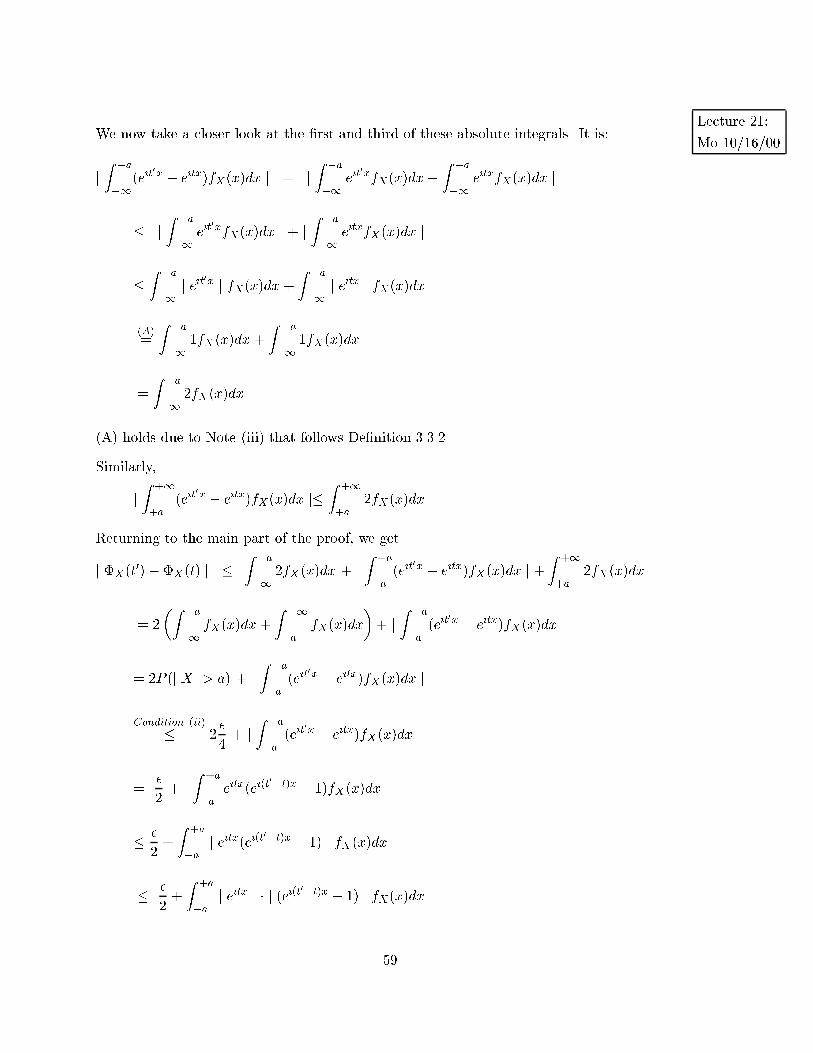
Lecture 21:

Mo 10/16/00We now take a closer look at the �rst and third of these absolute integrals. It is:

jZ �a

�1(e{t

0x � e{tx)fX(x)dx j = j

Z �a

�1e{t0x

fX(x)dx�Z �a

�1e{txfX(x)dx j

� jZ �a

�1e{t0x

fX(x)dx j + jZ �a

�1e{txfX(x)dx j

�Z �a

�1j e{t0x j fX(x)dx +

Z �a

�1j e{tx j fX(x)dx

(A)=

Z �a

�11fX(x)dx+

Z �a

�11fX(x)dx

=

Z �a

�12fX(x)dx.

(A) holds due to Note (iii) that follows De�nition 3.3.2.

Similarly,

jZ +1

+a(e{t

0x � e{tx)fX(x)dx j�

Z +1

+a2fX(x)dx

Returning to the main part of the proof, we get

j �X(t0)��X(t) j �

Z �a

�12fX(x)dx + j

Z +a

�a(e{t

0x � e{tx)fX(x)dx j +

Z +1

+a2fX(x)dx

= 2

�Z �a

�1fX(x)dx+

Z +1

+afX(x)dx

�+ j

Z +a

�a(e{t

0x � e{tx)fX(x)dx j

= 2P (j X j> a) + jZ +a

�a(e{t

0x � e{tx)fX(x)dx j

Condition (ii)

� 2�

4+ j

Z +a

�a(e{t

0x � e{tx)fX(x)dx j

=�

2+ j

Z +a

�ae{tx(e{(t

0�t)x � 1)fX(x)dx j

� �

2+

Z +a

�aj e{tx(e{(t0�t)x � 1) j fX(x)dx

� �

2+

Z +a

�aj e{tx j � j (e{(t0�t)x � 1) j fX(x)dx

59

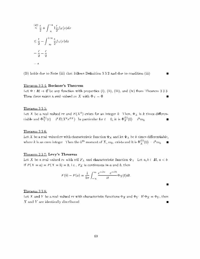
(B)

� �

2+

Z +a

�a1�

2fX(x)dx

� �

2+

Z +1

�1

�

2fX(x)dx

=�

2+�

2

= �

(B) holds due to Note (iii) that follows De�nition 3.3.2 and due to condition (iii).

Theorem 3.3.4: Bochner's Theorem

Let � : IR ! CI be any function with properties (i), (ii), (iii), and (iv) from Theorem 3.3.3.

Then there exists a real{valued rv X with �X = �.

Theorem 3.3.5:

Let X be a real{valued rv and E(Xk) exists for an integer k. Then, �X is k times di�eren-

tiable and �(k)X (t) = i

kE(Xk

eitX). In particular for t = 0, it is �

(k)X (0) = i

kmk.

Theorem 3.3.6:

Let X be a real{valued rv with characteristic function �X and let �X be k times di�erentiable,

where k is an even integer. Then the kth moment of X, mk, exists and it is �(k)X (0) = i

kmk.

Theorem 3.3.7: Levy's Theorem

Let X be a real{valued rv with cdf FX and characteristic function �X . Let a; b 2 IR, a < b.

If P (X = a) = P (X = b) = 0, i.e., FX is continuous in a and b, then

F (b)� F (a) =1

2�

Z 1

�1

e�ita � e

�itb

it�X(t)dt:

Theorem 3.3.8:

Let X and Y be a real{valued rv with characteristic functions �X and �Y . If �X = �Y , then

X and Y are identically distributed.

60

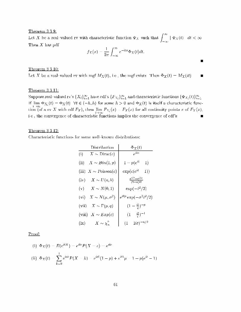
Theorem 3.3.9:

Let X be a real{valued rv with characteristic function �X such that

Z 1

�1j �X(t) j dt < 1.

Then X has pdf

fX(x) =1

2�

Z 1

�1e�itx�X(t)dt:

Theorem 3.3.10:

Let X be a real{valued rv with mgf MX(t), i.e., the mgf exists. Then �X(t) =MX(it).

Theorem 3.3.11:

Suppose real{valued rv's fXig1i=1 have cdf's fFXig1i=1 and characteristic functions f�Xi

(t)g1i=1.If lim

i!1�Xi

(t) = �X(t) 8t 2 (�h; h) for some h > 0 and �X(t) is itself a characteristic func-

tion (of a rv X with cdf FX), then limi!1

FXi(x) = FX(x) for all continuity points x of FX(x),

i.e., the convergence of characteristic functions implies the convergence of cdf's.

Theorem 3.3.12:

Characteristic functions for some well{known distributions:

Distribution �X(t)

(i) X � Dirac(c) eitc

(ii) X � Bin(1; p) 1 + p(eit � 1)

(iii) X � Poisson(c) exp(c(eit � 1))

(iv) X � U(a; b) eitb�eita(b�a)it

(v) X � N(0; 1) exp(�t2=2)

(vi) X � N(�; �2) eit� exp(��2t2=2)

(vii) X � �(p; q) (1� itq )�p

(viii) X � Exp(c) (1� itc )�1

(ix) X � �2n (1� 2it)�n=2

Proof:

(i) �X(t) = E(eitX ) = eitcP (X = c) = e

itc

(ii) �X(t) =1X

k=0

eitkP (X = k) = e

it0(1� p) + eit1p = 1 + p(eit � 1)

61

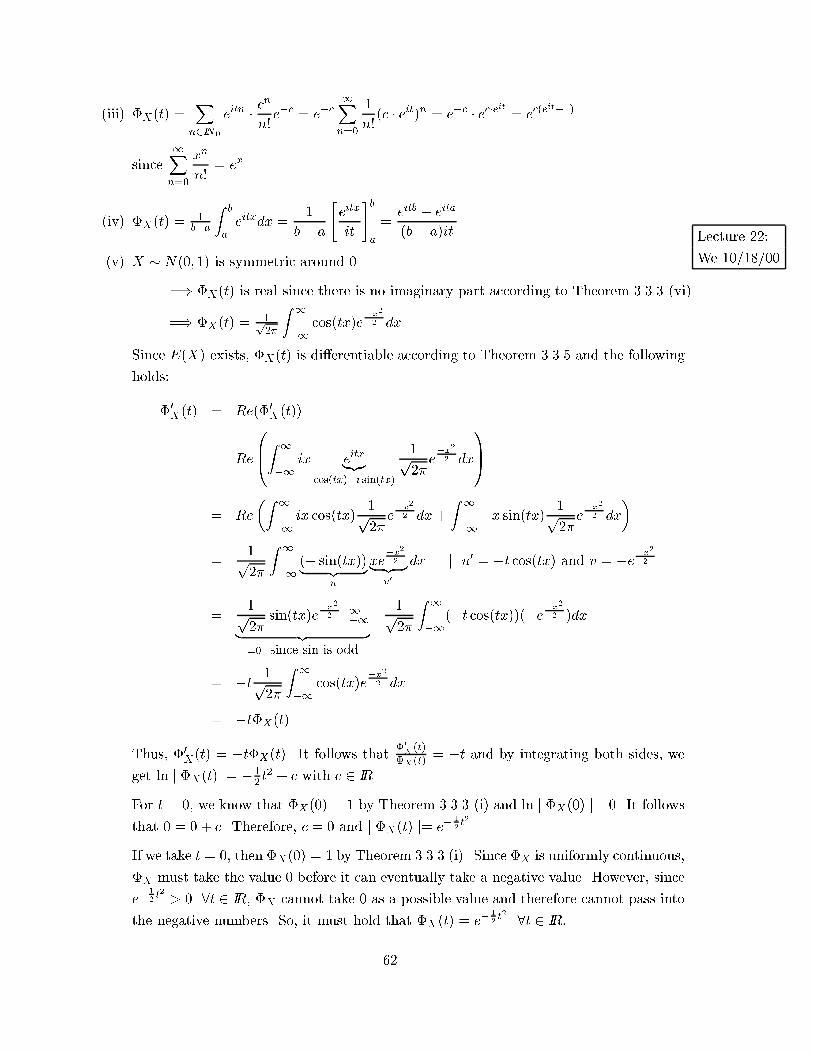
(iii) �X(t) =Xn2IN0

eitn � c

n

n!e�c = e

�c1Xn=0

1

n!(c � eit)n = e

�c � ec�eit = ec(eit�1)

since1Xn=0

xn

n!= e

x

(iv) �X(t) =1

b�a

Z b

aeitxdx =

1

b� a

"eitx

it

#ba

=eitb � e

ita

(b� a)it Lecture 22:

We 10/18/00(v) X � N(0; 1) is symmetric around 0

=) �X(t) is real since there is no imaginary part according to Theorem 3.3.3 (vi)

=) �X(t) =1p2�

Z 1

�1cos(tx)e

�x2

2 dx

Since E(X) exists, �X(t) is di�erentiable according to Theorem 3.3.5 and the following

holds:

�0X(t) = Re(�0X(t))

= Re

0B@Z 1

�1ix e

itx|{z}cos(tx)+i sin(tx)

1p2�

e�x2

2 dx

1CA

= Re

�Z 1

�1ix cos(tx)

1p2�

e�x2

2 dx+

Z 1

�1�x sin(tx) 1p

2�e�x2

2 dx

�

=1p2�

Z 1

�1(� sin(tx))| {z }

u

xe�x2

2| {z }v0

dx j u0 = �t cos(tx) and v = �e�x2

2

=1p2�

sin(tx)e�x2

2 j1�1| {z }=0 since sin is odd

� 1p2�

Z 1

�1(�t cos(tx))(�e

�x2

2 )dx

= �t 1p2�

Z 1

�1cos(tx)e

�x2

2 dx

= �t�X(t)

Thus, �0X(t) = �t�X(t). It follows that�0X(t)

�X(t) = �t and by integrating both sides, we

get ln j �X(t) j= �12 t2 + c with c 2 IR.

For t = 0, we know that �X(0) = 1 by Theorem 3.3.3 (i) and ln j �X(0) j= 0. It follows

that 0 = 0 + c. Therefore, c = 0 and j �X(t) j= e� 1

2t2 .

If we take t = 0, then �X(0) = 1 by Theorem 3.3.3 (i). Since �X is uniformly continuous,

�X must take the value 0 before it can eventually take a negative value. However, since

e� 12t2> 0 8t 2 IR, �X cannot take 0 as a possible value and therefore cannot pass into

the negative numbers. So, it must hold that �X(t) = e� 12t2 8t 2 IR:

62

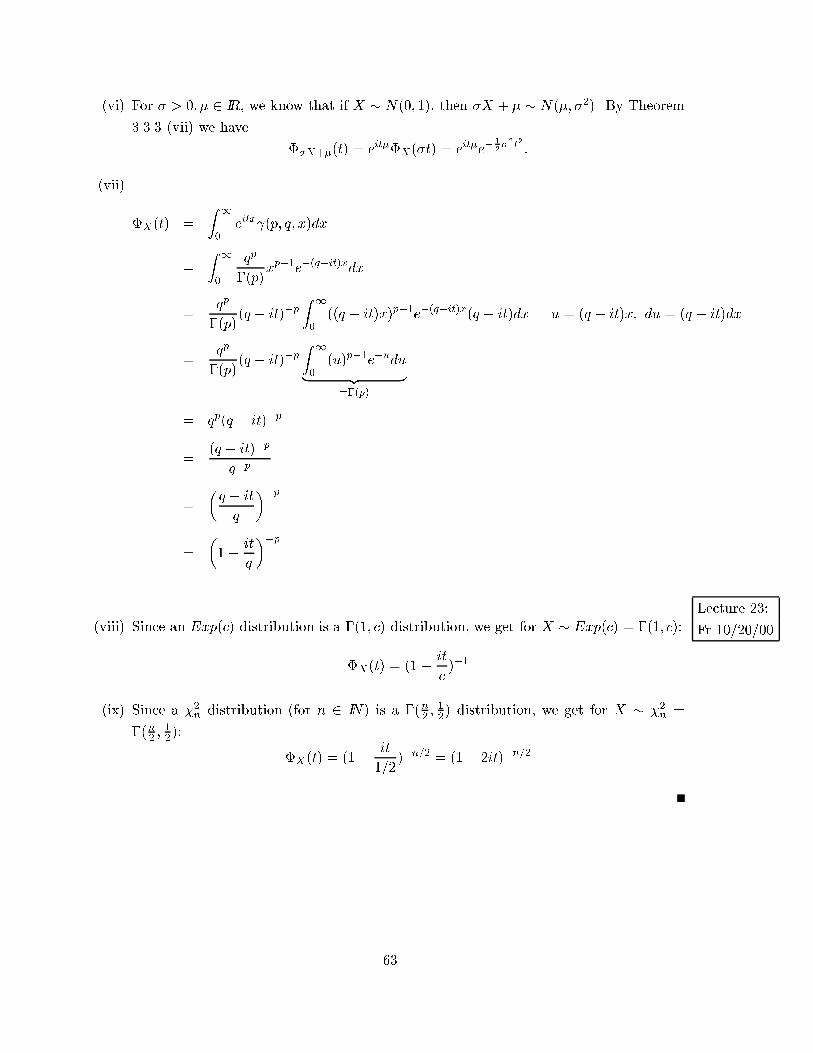
(vi) For � > 0; � 2 IR, we know that if X � N(0; 1), then �X + � � N(�; �2). By Theorem

3.3.3 (vii) we have

��X+�(t) = eit��X(�t) = e

it�e� 12�2t2

:

(vii)

�X(t) =

Z 1

0eitx (p; q; x)dx

=

Z 1

0

qp

�(p)xp�1

e�(q�it)x

dx

=qp

�(p)(q � it)�p

Z 1

0((q � it)x)p�1e�(q�it)x(q � it)dx j u = (q � it)x; du = (q � it)dx

=qp

�(p)(q � it)�p

Z 1

0(u)p�1e�udu| {z }=�(p)

= qp(q � it)�p

=(q � it)�p

q�p

=

�q � it

q

��p

=

�1� it

q

��p

Lecture 23:

Fr 10/20/00(viii) Since an Exp(c) distribution is a �(1; c) distribution, we get for X � Exp(c) = �(1; c):

�X(t) = (1� it

c)�1

(ix) Since a �2n distribution (for n 2 IN) is a �(n2 ;

12) distribution, we get for X � �

2n =

�(n2 ;12):

�X(t) = (1� it

1=2)�n=2 = (1� 2it)�n=2

63

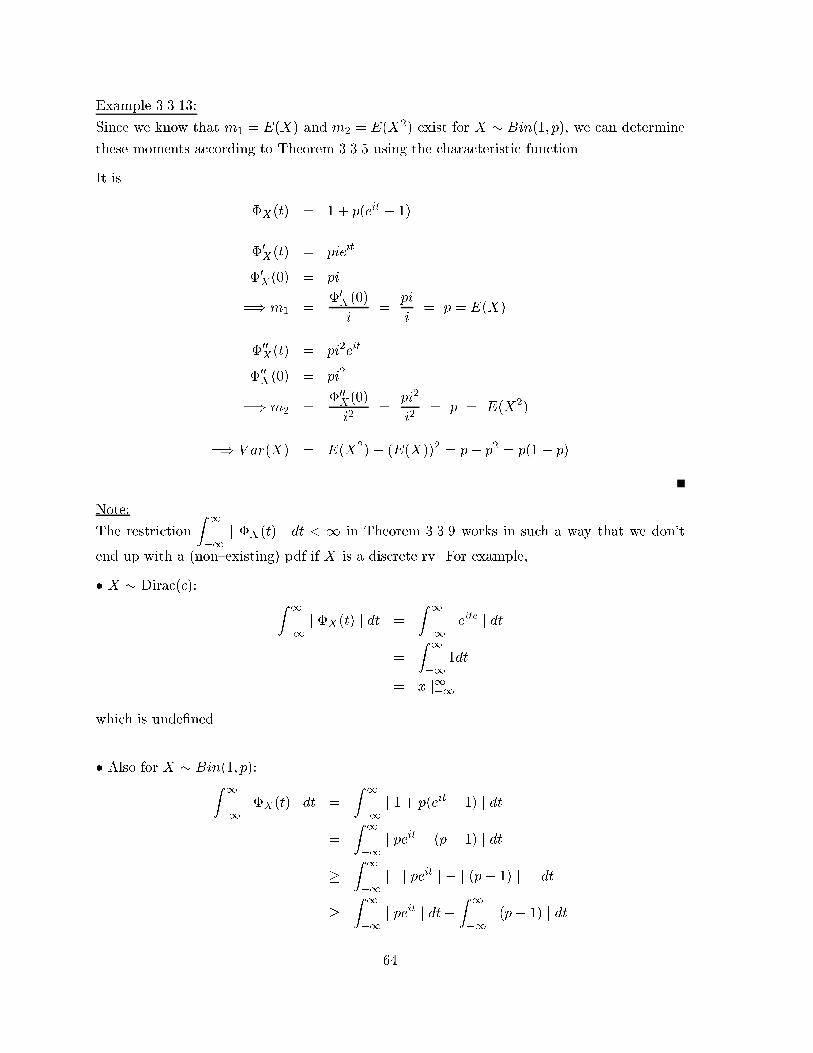
Example 3.3.13:

Since we know that m1 = E(X) and m2 = E(X2) exist for X � Bin(1; p), we can determine

these moments according to Theorem 3.3.5 using the characteristic function.

It is

�X(t) = 1 + p(eit � 1)

�0X(t) = pieit

�0X(0) = pi

=) m1 =�0X(0)

i=

pi

i= p = E(X)

�00X(t) = pi2eit

�00X(0) = pi2

=) m2 =�00X(0)i2

=pi2

i2= p = E(X2)

=) V ar(X) = E(X2)� (E(X))2 = p� p2 = p(1� p)

Note:

The restriction

Z 1

�1j �X(t) j dt < 1 in Theorem 3.3.9 works in such a way that we don't

end up with a (non{existing) pdf if X is a discrete rv. For example,

� X � Dirac(c): Z 1

�1j �X(t) j dt =

Z 1

�1j eitc j dt

=

Z 1

�11dt

= x j1�1

which is unde�ned.

� Also for X � Bin(1; p):Z 1

�1j �X(t) j dt =

Z 1

�1j 1 + p(eit � 1) j dt

=

Z 1

�1j peit � (p� 1) j dt

�Z 1

�1j j peit j � j (p� 1) j j dt

�Z 1

�1j peit j dt�

Z 1

�1j (p� 1) j dt

64

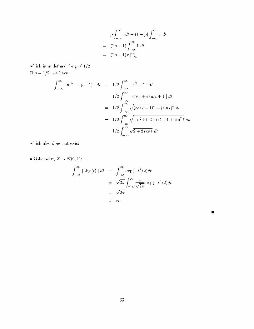
= p

Z 1

�11dt� (1� p)

Z 1

�11 dt

= (2p� 1)

Z 1

�11 dt

= (2p� 1)x j1�1

which is unde�ned for p 6= 1=2.

If p = 1=2, we have

Z 1

�1j peit � (p� 1) j dt = 1=2

Z 1

�1j eit + 1 j dt

= 1=2

Z 1

�1j cos t+ i sin t+ 1 j dt

= 1=2

Z 1

�1

q(cos t+ 1)2 + (sin t)2 dt

= 1=2

Z 1

�1

qcos2 t+ 2 cos t+ 1 + sin2 t dt

= 1=2

Z 1

�1

p2 + 2 cos t dt

which also does not exist.

� Otherwise, X � N(0; 1):

Z 1

�1j �X(t) j dt =

Z 1

�1exp(�t2=2)dt

=p2�

Z 1

�1

1p2�

exp(�t2=2)dt

=p2�

< 1

65

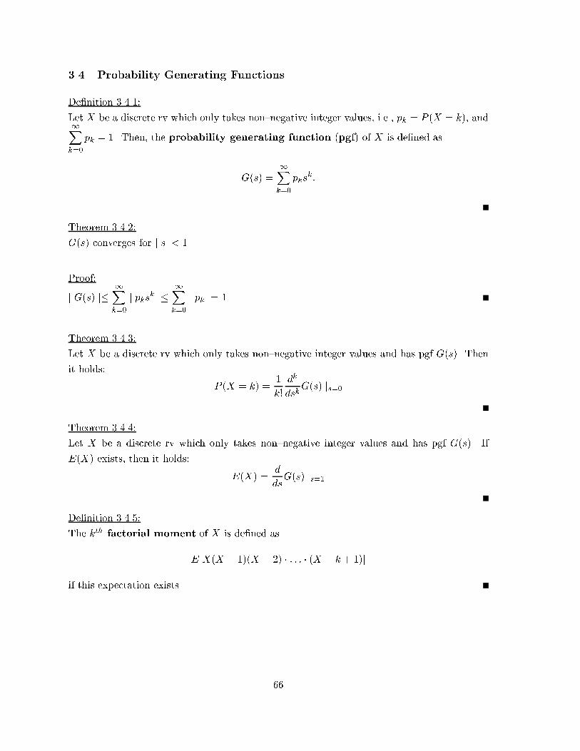
3.4 Probability Generating Functions

De�nition 3.4.1:

Let X be a discrete rv which only takes non{negative integer values, i.e., pk = P (X = k), and1Xk=0

pk = 1. Then, the probability generating function (pgf) of X is de�ned as

G(s) =1Xk=0

pksk:

Theorem 3.4.2:

G(s) converges for j s j< 1.

Proof:

j G(s) j�1Xk=0

j pksk j�1Xk=0

j pk j= 1

Theorem 3.4.3:

Let X be a discrete rv which only takes non{negative integer values and has pgf G(s). Then

it holds:

P (X = k) =1

k!

dk

dskG(s) js=0

Theorem 3.4.4:

Let X be a discrete rv which only takes non{negative integer values and has pgf G(s). If

E(X) exists, then it holds:

E(X) =d

dsG(s) js=1

De�nition 3.4.5:

The kth factorial moment of X is de�ned as

E[X(X � 1)(X � 2) � : : : � (X � k + 1)]

if this expectation exists.

66

Theorem 3.4.6:

Let X be a discrete rv which only takes non{negative integer values and has pgf G(s). If

E[X(X � 1)(X � 2) � : : : � (X � k + 1)] exists, then it holds:

E[X(X � 1)(X � 2) � : : : � (X � k + 1)] =dk

dskG(s) js=1

Note:

Similar to the Cauchy distribution for the continuous case, there exist discrete distributions

where the mean (or higher moments) do not exist. See Homework.

67

Lecture 24:

Mo 10/23/003.5 Moment Inequalities

Theorem 3.5.1:

Let h(X) be a non{negative Borel{measurable function of a rv X. If E(h(X)) exists, then it

holds:

P (h(X) � �) � E(h(X))

�8� > 0

Proof:

Continuous case only:

E(h(X)) =

Z 1

�1h(x)fX(x)dx

=

ZAh(x)fX(x)dx+

ZAC

h(x)fX(x)dx j where A = fx : h(x) � �g

�ZAh(x)fX(x)dx

�ZA�fX(x)dx

= �P (h(X) � �) 8� > 0

Therefore, P (h(X) � �) � E(h(X))�

8� > 0.

Corollary 3.5.2: Markov's Inequality

Let h(X) =j X jr and � = kr where r > 0 and k > 0. If E(j X jr) exists, then it holds:

P (j X j� k) � E(j X jr)kr

Proof:

Since P (j X j� k) = P (j X jr� kr) for k > 0, it follows using Theorem 3.5.1:

P (j X j� k) = P (j X jr� kr)

Th:3:5:1� E(j X jr)

kr

Corollary 3.5.3: Chebychev's Inequality

Let h(X) = (X � �)2 and � = k2�2 where E(X) = �, V ar(X) = �

2<1, and k > 0. Then it

holds:

P (j X � � j> k�) � 1

k2

68

Proof:

Since P (j X � � j> k�) = P (j X � � j2> k2�2) for k > 0, it follows using Theorem 3.5.1:

P (j X � � j> k�) = P (j X � � j2> k2�2)

Th:3:5:1� E(j X � � j2)

k2�2=

V ar(X)

k2�2=

�2

k2�2=

1

k2

Theorem 3.5.4: Lyapunov's Inequality

Let 0 < �n = E(j X jn) <1. For arbitrary k such that 2 � k � n, it holds that

(�k�1)1

k�1 � (�k)1k ;

i.e., (E(j X jk�1))1

k�1 � (E(j X jk)) 1k .

Proof:

Continuous case only:

Let Q(u; v) = E

�(u j X j

k�12 +v j X j

k+12 )2

�. Obviously, Q(u; v) � 0 8u; v 2 IR. Also,

Q(u; v) =

Z 1

�1(u j x j

k�12 +v j x j

k+12 )2fX(x)dx

= u2Z 1

�1j x jk�1 fX(x)dx+ 2uv

Z 1

�1j x jk fX(x)dx+ v

2Z 1

�1j x jk+1 fX(x)dx

= u2�k�1 + 2uv�k + v

2�k+1

� 0 8u; v 2 IR

Using the fact that Ax2 + 2Bxy + Cy2 � 0 8x; y 2 IR i� A > 0 and AC � B

2> 0 (see

Rohatgi, page 6, Section P2.4), we get with A = �k�1; B = �k, and C = �k+1:

�k�1�k+1 � �2k � 0

=) �2k � �k�1�k+1

=) �2kk � �

kk�1�

kk+1

This means that �21 � �0�2, �42 � �

21�

23 , �

63 � �

32�

34 , and so on. Multiplying these, we get:

k�1Yj=1

�2jj �

k�1Yj=1

�jj�1�

jj+1

= (�0�2)(�21�

23)(�

32�

34)(�

43�

45) : : : (�

k�2k�3�

k�2k�1)(�

k�1k�2�

k�1k )

= �0�k�2k�1�

k�1k

k�2Yj=1

�2jj

69

Dividing both sides byk�2Yj=1

�2jj , we get:

�2k�2k�1 � �0�

k�1k �

k�2k�1

�0=1=) �

kk�1 � �

k�1k

=) �1k�1 � �

k�1k

k

=) �

1k�1

k�1 � �

1k

k

70

Lecture 25:

We 10/25/00

4 Random Vectors

4.1 Joint, Marginal, and Conditional Distributions

De�nition 4.1.1:

The vectorX = (X1; : : : ;Xn)0 on (; L; P )! IR

n de�ned byX(!) = (X1(!); : : : ;Xn(!))0; ! 2

, is an n{dimensional random vector (n{rv) if X�1(I) = f! : X1(!) � a1; : : : ; Xn(!) �ang 2 L for all n{dimensional intervals I = f(x1; : : : ; xn) : �1 < xi � ai; ai 2 IR 8i =1; : : : ; ng.

Note:

It follows that if X1; : : : ; Xn are any n rv's on (; L; P ), then X = (X1; : : : ;Xn)0 is an n{rv

on (; L; P ) since for any I, it holds:

X�1(I) = f! : (X1(!); : : : ; Xn(!)) 2 Ig

= f! : X1(!) � a1; : : : ;Xn(!) � ang

=n\

k=1

f! : Xk(!) � akg| {z }2L| {z }

2L

De�nition 4.1.2:

For an n{rv X , a function F de�ned by

F (x) = P (X � x) = P (X1 � x1; : : : ; Xn � xn) 8x 2 IRn

is the joint cumulative distribution function (joint cdf) of X .

Note:

(i) F is non{decreasing and right{continuous in each of its arguments xi.

(ii) limx!1F (x) = lim

x1!1;:::xn!1F (x) = 1 and limxk!�1

F (x) = 0 8x1; : : : ; xk�1; xk+1; : : : ; xn 2IR.

However, conditions (i) and (ii) together are not su�cient for F to be a joint cdf. Instead we

need the conditions from the next Theorem.

71

Theorem 4.1.3:

A function F (x) = F (x1; : : : ; xn) is the joint cdf of some n{rv X i�

(i) F is non{decreasing and right{continuous with respect to each xi,

(ii) F (�1; x2; : : : ; xn) = F (x1;�1; x3; : : : ; xn) = : : : = F (x1; : : : ; xn�1;�1) = 0 and

F (1; : : : ;1) = 1, and

(iii) 8x 2 IRn 8�i > 0; i = 1; : : : n, the following inequality holds:

F (x+ �) �nXi=1

F (x1 + �1; : : : ; xi�1 + �i�1; xi; xi+1 + �i+1; : : : ; xn + �n)

+X

1�i<j�nF (x1 + �1; : : : ; xi�1 + �i�1; xi; xi+1 + �i+1; : : : ;

xj�1 + �j�1; xj ; xj+1 + �j+1; : : : ; xn + �n)

� : : :

+ (�1)nF (x)

� 0

Note:

We won't prove this Theorem but just see why we need condition (iii) for n = 2:

P (x1 < X � x2; y1 < Y � y2) =

P (X � x2; Y � y2)�P (X � x1; Y � y2)�P (X � x2; Y � y1)+P (X � x1; Y � y1) � 0

Note:

We will restrict ourselves to n = 2 for most of the next De�nitions and Theorems but those

can be easily generalized to n > 2. The term bivariate rv is often used to refer to a 2{rv

and multivariate rv is used to refer to an n{rv, n � 2.

De�nition 4.1.4:

A 2{rv (X;Y ) is discrete if there exists a countable collection X of pairs (xi; yi) that has

probability 1. Let pij = P (X = xi; Y = yj) > 0 8(xi; yj) 2 X. Then,Xi;j

pij = 1 and fpijg is

the joint probability mass function (joint pmf) of (X;Y ).

72

De�nition 4.1.5:

Let (X;Y ) be a discrete 2{rv with joint pmf fpijg. De�ne

pi� =1Xj=1

pij =1Xj=1

P (X = xi; Y = yj) = P (X = xi)

and

p�j =1Xi=1

pij =1Xi=1

P (X = xi; Y = yj) = P (Y = yj):

Then fpi�g is called the marginal probability mass function (marginal pmf) of X and

fp�jg is called the marginal probability mass function of Y .

De�nition 4.1.6:

A 2{rv (X;Y ) is continuous if there exists a non{negative function f such that

F (x; y) =

Z x

�1

Z y

�1f(u; v) dv du 8(x; y) 2 IR

2

where F is the joint cdf of (X;Y ). We call f the joint probability density function (joint

pdf) of (X;Y ).

Note:

If F is continuous at (x; y), then

d2F (x; y)

dx dy= f(x; y):

De�nition 4.1.7:

Let (X;Y ) be a continuous 2{rv with joint pdf f . Then fX(x) =

Z 1

�1f(x; y)dy is called the

marginal probability density function (marginal pdf) of X and fY (y) =

Z 1

�1f(x; y)dx

is called the marginal probability density function of Y .

Note:

(i)

Z 1

�1fX(x)dx =

Z 1

�1

�Z 1

�1f(x; y)dy

�dx = F (1;1) = 1 =

Z 1

�1

�Z 1

�1f(x; y)dx

�dy =

Z 1

�1fY (y)dy

and fX(x) � 0 8x 2 IR and fY (y) � 0 8y 2 IR.

73

(ii) Given a 2{rv (X;Y ) with joint cdf F (x; y), how do we generate a marginal cdf

FX(x) = P (X � x) ? | The answer is P (X � x) = P (X � x;�1 < Y < 1) =

F (x;1).

De�nition 4.1.8:

If FX(x1; : : : ; xn) = FX(x) is the joint cdf of an n{rv X = (X1; : : : ;Xn), then the marginal

cumulative distribution function (marginal cdf) of (Xi1 ; : : : ; Xik); 1 � k � n � 1; 1 �i1 < i2 < : : : < ik � n, is given by

limxi!1;i 6=i1;:::;ik

FX(x) = FX(1; : : : ;1; xi1 ;1; : : : ;1; xi2 ;1; : : : ;1; xik ;1; : : : ;1):

Note:

In De�nition 1.4.1, we de�ned conditional probability distributions in some probability space

(; L; P ). This de�nition extends to conditional distributions of 2{rv's (X;Y ).

De�nition 4.1.9:

Let (X;Y ) be a discrete 2{rv. If P (Y = yj) = p�j > 0, then the conditional probability

mass function (conditional pmf) of X given Y = yj (for �xed j) is de�ned as

pijj = P (X = xi j Y = yj) =P (X = xi; Y = yj)

P (Y = yj)=

pij

p�j:

Note:

For a continuous 2{rv (X;Y ) with pdf f , P (X � x j Y = y) is not de�ned. Let � > 0 and

suppose that P (y� � < Y � y+ �) > 0. For every x and every interval (y� �; y+ �], consider

the conditional probability of X � x given Y 2 (y � �; y + �]. We have

P (X � x j y � � < Y � y + �) =P (X � x; y � � < Y � y + �)

P (y � � < Y � y + �)

which is well{de�ned if P (y � � < Y � y + �) > 0 holds.

So, when does

lim�!0+

P (X � x j Y 2 (y � �; y + �])

exist? See the next de�nition.

74

De�nition 4.1.10:

The conditional cumulative distribution function (conditional cdf) of a rv X given

that Y = y is de�ned to be

FXjY (x j y) = lim�!0+

P (X � x j Y 2 (y � �; y + �])

provided that this limit exists. If it does exist, the conditional probability density func-

tion (conditional pdf) of X given that Y = y is any non{negative function fXjY (x j y)satisfying

FXjY (x j y) =Z x

�1fXjY (t j y)dt 8x 2 IR:

Note:

For �xed y, fXjY (x j y) � 0 and

Z 1

�1fXjY (x j y)dx = 1. So it is really a pdf.

Theorem 4.1.11:

Let (X;Y ) be a continuous 2{rv with joint pdf fX;Y . It holds that at every point (x; y) where

f is continuous and the marginal pdf fY (y) > 0, we have

FXjY (x j y) = lim�!0+

P (X � x; Y 2 (y � �; y + �])

P (Y 2 (y � �; y + �])

= lim�!0+

0BBB@

12�

Z x

�1

Z y+�

y��fX;Y (u; v)dv du

12�

Z y+�

y��fY (v)dv

1CCCA

=

Z x

�1fX;Y (u; y)du

fY (y)

=

Z x

�1

fX;Y (u; y)

fY (y)du:

Thus, fXjY (x j y) exists and equalsfX;Y (x;y)

fY (y), provided that fY (y) > 0. Furthermore, since

Z x

�1fX;Y (u; y)du = fY (y)FXjY (x j y);

we get the following marginal cdf of X:

FX(x) =

Z 1

�1

�Z x

�1fX;Y (u; y)du

�dy =

Z 1

�1fY (y)FXjY (x j y)dy

75

Lecture 26:

Fr 10/27/00Example 4.1.12:

Consider

fX;Y (x; y) =

(2; 0 < x < y < 1

0; otherwise

We calculate the marginal pdf's fX(x) and fY (y) �rst:

fX(x) =

Z 1

�1fX;Y (x; y)dy =

Z 1

x2dy = 2(1� x) for 0 < x < 1

and

fY (y) =

Z 1

�1fX;Y (x; y)dx =

Z y

02dx = 2y for 0 < y < 1

The conditional pdf's fY jX(y j x) and fXjY (x j y) are calculated as follows:

fY jX(y j x) =fX;Y (x; y)

fX(x)=

2

2(1� x)=

1

1� xfor x < y < 1 (where 0 < x < 1)

and

fXjY (x j y) =fX;Y (x; y)

fY (y)=

2

2y=

1

yfor 0 < x < y (where 0 < y < 1)

Thus, it holds that Y j X = x � U(x; 1) and X j Y = y � U(0; y), i.e., both conditional pdf's

are related to uniform distributions.

76

4.2 Independent Random Variables

Example 4.2.1: (from Rohatgi, page 119, Example 1)

Let f1; f2; f3 be 3 pdf's with cdf's F1; F2; F3 and let j � j� 1. De�ne

f�(x1; x2; x3) = f1(x1)f2(x2)f3(x3) � (1 + �(2F1(x1)� 1)(2F2(x2)� 1)(2F3(x3)� 1)):

We can show

(i) f� is a pdf for all � 2 [�1; 1].

(ii) ff� : �1 � � � 1g all have marginal pdf's f1; f2; f3.

See book for proof and further discussion | but when do the marginal distributions uniquely

determine the joint distribution?

De�nition 4.2.2:

Let FX;Y (x; y) be the joint cdf and FX(x) and FY (y) be the marginal cdf's of a 2{rv (X;Y ).

X and Y are independent i�

FX;Y (x; y) = FX(x)FY (y) 8(x; y) 2 IR2:

Lemma 4.2.3:

If X and Y are independent, a; b; c; d 2 IR, and a < b and c < d, then

P (a < X � b; c < Y � d) = P (a < X � b)P (c < Y � d):

Proof:

P (a < X � b; c < Y � d) = FX;Y (b; d) � FX;Y (a; d) � FX;Y (b; c) + FX;Y (a; c)

= FX(b)FY (d)� FX(a)FY (d)� FX(b)FY (c) + FX(a)FY (c)

= (FX(b)� FX(a))(FY (d)� FY (c))

= P (a < X � b)P (c < Y � d)

De�nition 4.2.4:

A collection of rv's X1; : : : ;Xn with joint cdf FX(x) and marginal cdf's FXi(xi) aremutually

(or completely) independent i�

FX(x) =nYi=1

FXi(xi) 8x 2 IR

n:

77

Note:

We often simply say that the rv's X1; : : : ;Xn are independent when we really mean that

they are mutually independent.

Theorem 4.2.5: Factorization Theorem

(i) A necessary and su�cient condition for discrete rv's X1; : : : ;Xn to be independent is

that

P (X = x) = P (X1 = x1; : : : ;Xn = xn) =nYi=1

P (Xi = xi) 8x 2 X

where X � IRn is the countable support of X .

(ii) For an absolutely continuous n{rv X = (X1; : : : ;Xn), X1; : : : ;Xn are independent i�

fX(x) = fX1;:::;Xn(x1; : : : ; xn) =nYi=1

fXi(xi);

where fX is the joint pdf and fX1; : : : ; fXn are the marginal pdfs of X.

Proof:

(i) Discrete case:

Let X be a random vector whose components are independent random variables of the

discrete type with P (X = b) > 0. Lemma 4.2.3 extends to:

lima"b

P (a < X � b) = limai"bi 8i2f1;:::;ng

P (a1 < X1 � b1; a2 < X2 � b2; : : : ; an < Xn � bn)

= P (X1 = b1; X2 = b2; : : : ; Xn = bn)

= P (X = b)

indep:=

nYi=1

P (Xi = bi)

Before considering the converse factorization of the joint cdf of an n-rv, recall that

independence allows each value in the support of a component to combine with each

of all possible combinations of the other component values: a 3-dimensional vector

where the �rst component has support fx1a; x1b; x1cg, the second component has supportfx2a; x2b; x2cg, and the third component has support fx3a; x3b; x3cg, has 3� 3� 3 = 27

points in its support. Due to independence, all these vectors can be arranged into three

sets: the �rst set having x1a, the second set having x1b, and the third set having x1c,

with each set having 9 combinations of x2 and x3.

78

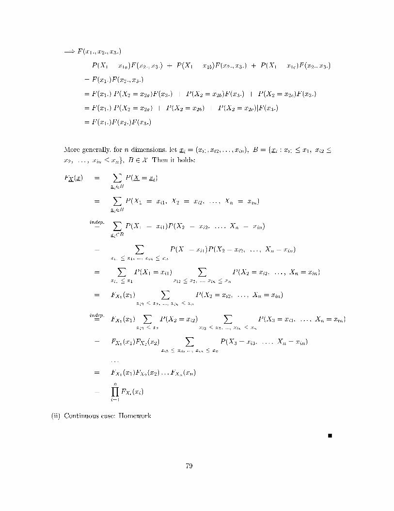
=) F (x1:; x2:; x3:)

= P (X1 = x1a)F (x2:; x3:) + P (X1 = x1b)F (x2:; x3:) + P (X1 = x1c)F (x2:; x3:)

= F (x1:)F (x2:; x3:)

= F (x1:)[P (X2 = x2a)F (x3:) + P (X2 = x2b)F (x3:) + P (X2 = x2c)F (x3:)]

= F (x1:)[P (X2 = x2a) + P (X2 = x2b) + P (X2 = x2c)]F (x3:)

= F (x1:)F (x2:)F (x3:)

More generally, for n dimensions, let xi = (xi1; xi2; : : : ; xin); B = fxi : xi1 � x1; xi2 �x2; : : : ; xin � xng; B 2 X. Then it holds:

FX(x) =Xxi2B

P (X = xi)

=Xxi2B

P (X1 = xi1; X2 = xi2; : : : ; Xn = xin)

indep:=

Xxi2B

P (X1 = xi1)P (X2 = xi2; : : : ; Xn = xin)

=X

xi1 � x1; :::; xin � xn

P (X1 = xi1)P (X2 = xi2; : : : ; Xn = xin)

=X

xi1 � x1

P (X1 = xi1)X

xi2 � x2; :::; xin � xn

P (X2 = xi2; : : : ; Xn = xin)

= FX1(x1)

Xxi2 � x2; :::; xin � xn

P (X2 = xi2; : : : ; Xn = xin)

indep:= FX1

(x1)X

xi2 � x2

P (X2 = xi2)X

xi3 � x3; :::; xin � xn

P (X3 = xi3; : : : ; Xn = xin)

= FX1(x1)FX2

(x2)X

xi3 � x3; :::; xin � xn

P (X3 = xi3; : : : ; Xn = xin)

= : : :

= FX1(x1)FX2

(x2) : : : FXn(xn)

=nYi=1

FXi(xi)

(ii) Continuous case: Homework

79

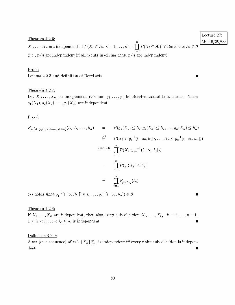
Lecture 27:

Mo 10/30/00Theorem 4.2.6:

X1; : : : ;Xn are independent i� P (Xi 2 Ai; i = 1; : : : ; n) =nYi=1

P (Xi 2 Ai) 8 Borel sets Ai 2 B

(i.e., rv's are independent i� all events involving these rv's are independent).

Proof:

Lemma 4.2.3 and de�nition of Borel sets.

Theorem 4.2.7:

Let X1; : : : ; Xn be independent rv's and g1; : : : ; gn be Borel{measurable functions. Then

g1(X1); g2(X2); : : : ; gn(Xn) are independent.

Proof:

Fg1(X1);g2(X2);:::;gn(Xn)(h1; h2; : : : ; hn) = P (g1(X1) � h1; g2(X2) � h2; : : : ; gn(Xn) � hn)

(�)= P (X1 2 g

�11 ((�1; h1]); : : : ;Xn 2 g

�1n ((�1; hn]))

Th:4:2:6=

nYi=1

P (Xi 2 g�1i ((�1; hi]))

=nYi=1

P (gi(Xi) � hi)

=nYi=1

Fgi(Xi)(hi)

(�) holds since g�11 ((�1; h1]) 2 B; : : : ; g�1n ((�1; hn]) 2 B

Theorem 4.2.8:

If X1; : : : ;Xn are independent, then also every subcollection Xi1 ; : : : ;Xik ; k = 2; : : : ; n � 1,

1 � i1 < i2 : : : < ik � n, is independent.

De�nition 4.2.9:

A set (or a sequence) of rv's fXng1n=1 is independent i� every �nite subcollection is indepen-

dent.

80

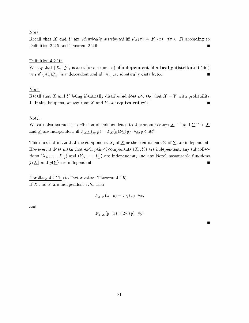
Note:

Recall that X and Y are identically distributed i� FX(x) = FY (x) 8x 2 IR according to

De�nition 2.2.5 and Theorem 2.2.6.

De�nition 4.2.10:

We say that fXng1n=1 is a set (or a sequence) of independent identically distributed (iid)

rv's if fXng1n=1 is independent and all Xn are identically distributed.

Note:

Recall that X and Y being identically distributed does not say that X = Y with probability

1. If this happens, we say that X and Y are equivalent rv's.

Note:

We can also extend the de�ntion of independence to 2 random vectors Xn�1 and Yn�1: X

and Y are independent i� FX;Y (x; y) = FX(x)FY (y) 8x; y 2 IRn.

This does not mean that the components Xi of X or the components Yi of Y are independent.

However, it does mean that each pair of components (Xi; Yi) are independent, any subcollec-

tions (Xi1 ; : : : ;Xik) and (Yj1 ; : : : ; Yjl) are independent, and any Borel{measurable functions

f(X) and g(Y ) are independent.

Corollary 4.2.11: (to Factorization Theorem 4.2.5)

If X and Y are independent rv's, then

FXjY (x j y) = FX(x) 8x;

and

FY jX(y j x) = FY (y) 8y:

81

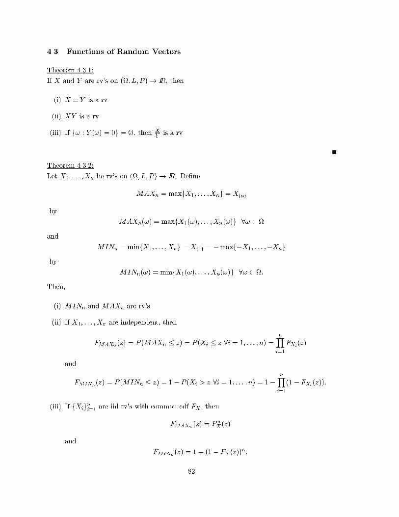
4.3 Functions of Random Vectors

Theorem 4.3.1:

If X and Y are rv's on (; L; P )! IR, then

(i) X � Y is a rv.

(ii) XY is a rv.

(iii) If f! : Y (!) = 0g = �, then XY is a rv.

Theorem 4.3.2:

Let X1; : : : ; Xn be rv's on (; L; P )! IR. De�ne

MAXn = maxfX1; : : : ;Xng = X(n)

by

MAXn(!) = maxfX1(!); : : : ; Xn(!)g 8! 2

and

MINn = minfX1; : : : ; Xng = X(1) = �maxf�X1; : : : ;�Xng

by

MINn(!) = minfX1(!); : : : ;Xn(!)g 8! 2 :

Then,

(i) MINn and MAXn are rv's.

(ii) If X1; : : : ;Xn are independent, then

FMAXn(z) = P (MAXn � z) = P (Xi � z 8i = 1; : : : ; n) =nYi=1

FXi(z)

and

FMINn(z) = P (MINn � z) = 1� P (Xi > z 8i = 1; : : : ; n) = 1�nYi=1

(1� FXi(z)):

(iii) If fXigni=1 are iid rv's with common cdf FX , then

FMAXn(z) = FnX(z)

and

FMINn(z) = 1� (1� FX(z))n:

82

If FX is absolutely continuous with pdf fX , then the pdfs of MAXn and MINn are

fMAXn(z) = n � F n�1X (z) � fX(z)

and

fMINn(z) = n � (1� FX(z))n�1 � fX(z)

for all continuity points of FX .

Note:

Using Theorem 4.3.2, it is easy to derive the joint cdf and pdf of MAXn and MINn for iid

rv's fX1; : : : ;Xng. For example, if the Xi's are iid with cdf FX and pdf fX , then the joint

pdf of MAXn and MINn is

fMAXn;MINn(x; y) =

(0; x � y

n(n� 1) � (FX (x)� FX(y))n�2 � fX(x)fX(y); x > y

However, note thatMAXn andMINn are not independent. See Rohatgi, page 129, Corollary,

for more details.

Note:

The previous transformations are special cases of the following Theorem 4.3.3.

Theorem 4.3.3:

If g : IRn ! IRm is a Borel{measurable function (i.e., 8B 2 Bm : g�1(B) 2 Bn) and if

X = (X1; : : : ;Xn) is an n{rv, then g(X) is an m{rv.

Proof:

If B 2 Bm, then f! : g(X(!)) 2 Bg = f! : X(!) 2 g�1(B)g 2 Bn.

Question: How do we handle more general transformations of X ?

Discrete Case:

Let X = (X1; : : : ;Xn) be a discrete n{rv and X � IRn be the countable support of X , i.e.,

P (X 2 X) = 1 and P (X = x) > 0 8x 2 X.

De�ne ui = gi(x1; : : : ; xn); i = 1; : : : ; n to be 1{to{1-mappings of X onto B. Let u =

(u1; : : : ; un)0. Then

P (U = u) = P (g1(X) = u1; : : : ; gn(X) = un) = P (X1 = h1(u); : : : ; Xn = hn(u)) 8u 2 B

83

where xi = hi(u); i = 1; : : : ; n, is the inverse transformation (and P (U = u) = 0 8u 62 B).

The joint marginal pmf of any subcollection of ui's is now obtained by summing over the other

remaining uj 's.

Example 4.3.4:

Let X;Y be iid � Bin(n; p); 0 < p < 1. Let U = XY+1 and V = Y + 1.

Then X = UV and Y = V � 1. So the joint pmf of U; V is

P (U = u; V = v) =

n

uv

!puv(1� p)n�uv

n

v � 1

!pv�1(1� p)n+1�v

=

n

uv

! n

v � 1

!puv+v�1(1� p)2n+1�uv�v

for v 2 f1; 2; : : : ; n+ 1g and uv 2 f0; 1; : : : ; ng.

Lecture 28:

We 11/01/00Continuous Case:

Let X = (X1; : : : ;Xn) be a continuous n{rv with joint cdf FX and joint pdf fX .

Let

U =

0BB@

U1

...

Un

1CCA = g(X) =

0BB@

g1(X)...

gn(X)

1CCA ;

i.e., Ui = gi(X), be a mapping from IRn into IRn.

If B 2 Bn, then

P (U 2 B) = P (X 2 g�1(B)) =

R: : :R

g�1(B)fX(x)d(x) =

R: : :R

g�1(B)fX(x)

nYi=1

dxi

where g�1(B) = fx = (x1; : : : ; xn) 2 IRn : g(x) 2 Bg.

Suppose we de�ne B as the half{in�nite n{dimensional interval

Bu = f(u01; : : : ; u0n) : �1 < u0i < ui 8i = 1; : : : ; ng

for any u 2 IRn. Then the joint cdf of U is

G(u) = P (U 2 Bu) = P (g1(X) � u1; : : : ; gn(X) � un) =

R: : :R

g�1(Bu)fX(x)d(x):

84

If G happens to be absolutely continuous, the joint pdf of U will be given by fU (u) =@nG(u)

@u1@u2:::@unat every continuity point of fU .

Under certain conditions, we can write fU in terms of the original pdf fX of X as stated in

the next Theorem:

Theorem 4.3.5: Multivariate Transformation

Let X = (X1; : : : ;Xn) be a continuous n{rv with joint pdf fX .

(i) Let

U =

0BB@

U1

...

Un

1CCA = g(X) =

0BB@

g1(X)...

gn(X)

1CCA ;

(i.e., Ui = gi(X)) be a 1{to{1{mapping from IRn into IR

n, i.e., there exist inverses hi,

i = 1; : : : ; n, such that xi = hi(u) = hi(u1; : : : ; un); i = 1; : : : ; n, over the range of the

transformation g.

(ii) Assume both g and h are continuous.

(iii) Assume partial derivatives @xi@uj

=@hi(u)@uj

; i; j = 1; : : : ; n, exist and are continuous.

(iv) Assume that the Jacobian of the inverse transformation

J = det

�@(x1; : : : ; xn)

@(u1; : : : ; un)

�= det

0BB@

@x1@u1

: : :@x1@un

......

@xn@u1

: : :@xn@un

1CCA =

��������

@x1@u1

: : :@x1@un

......

@xn@u1

: : :@xn@un

��������is di�erent from 0 for all u in the range of g.

Then the n{rv U = g(X) has a joint absolutely continuous cdf with corresponding joint pdf

fU(u) =j J j fX(h1(u); : : : ; hn(u)):

Proof:

Let u 2 IRn and

Bu = f(u01; : : : ; u0n) : �1 < u0i < ui 8i = 1; : : : ; ng:

Then,

GU(u) =

R: : :R

g�1(Bu)fX(x)d(x)

=

R: : :R

BufX(h1(u); : : : ; hn(u)) j J j d(u)

85

The result follows from di�erentiation of GU .

For additional steps of the proof see Rohatgi (page 135 and Theorem 17 on page 10) or a book

on multivariate calculus.

Theorem 4.3.6:

Let X = (X1; : : : ;Xn) be a continuous n{rv with joint pdf fX .

(i) Let

U =

0BB@

U1

...

Un

1CCA = g(X) =

0BB@

g1(X)...

gn(X)

1CCA ;

(i.e., Ui = gi(X)) be a mapping from IRn into IRn.

(ii) Let X = fx : fX(x) > 0g be the support of X .

(iii) Suppose that for each u 2 B = fu 2 IRn : u = g(x) for some x 2 Xg there is a �nite

number k = k(u) of inverses.

(iv) Suppose we can partition X into X0;X1; : : : ;Xk s.t.

(a) P (X 2 X0) = 0.

(b) U = g(X) is a 1{to{1{mapping from Xl onto B for all l = 1; : : : ; k, with inverse

transformation hl(u) =

0BB@

hl1(u)...

hln(u)

1CCA ; u 2 B, i.e., for each u 2 B, hl(u) is the unique

x 2 Xl such that u = g(x).

(v) Assume partial derivatives @xi@uj

=@hli(u)@uj

; l = 1; : : : ; k; i; j = 1; : : : ; n, exist and are

continuous.

(vi) Assume the Jacobian of each of the inverse transformations

Jl = det

0BB@

@x1@u1

: : :@x1@un

......

@xn@u1

: : :@xn@un

1CCA = det

0BB@

@hl1@u1

: : :@hl1@un

......

@hln@u1

: : :@hln@un

1CCA =

��������

@hl1@u1

: : :@hl1@un

......

@hln@u1

: : :@hln@un

��������; l = 1; : : : ; k;

is di�erent from 0 for all u in the range of g.

Then the joint pdf of U is given by

fU (u) =kXl=1

j Jl j fX(hl1(u); : : : ; hln(u)):

86

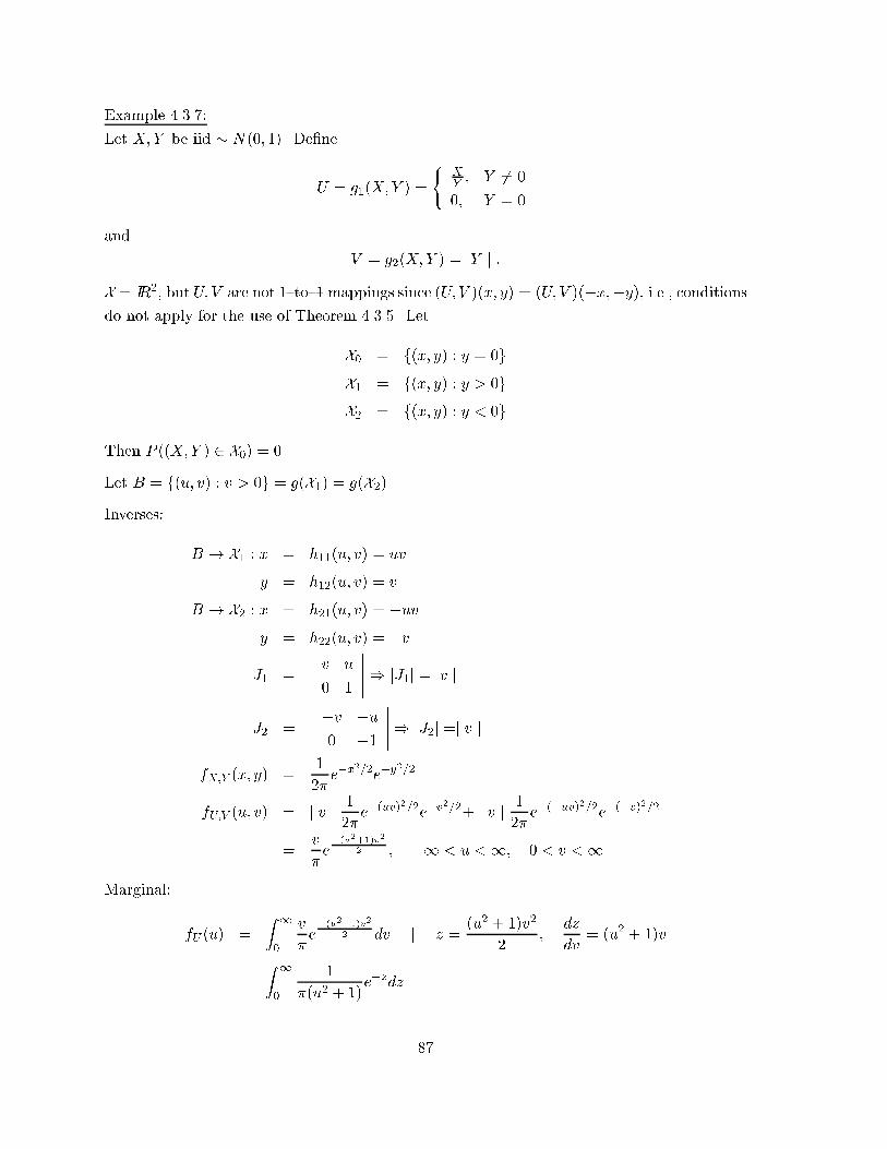
Example 4.3.7:

Let X;Y be iid � N(0; 1). De�ne

U = g1(X;Y ) =

(XY ; Y 6= 0

0; Y = 0

and

V = g2(X;Y ) =j Y j :

X = IR2, but U; V are not 1{to{1 mappings since (U; V )(x; y) = (U; V )(�x;�y), i.e., conditions

do not apply for the use of Theorem 4.3.5. Let

X0 = f(x; y) : y = 0g

X1 = f(x; y) : y > 0g

X2 = f(x; y) : y < 0g

Then P ((X;Y ) 2 X0) = 0.

Let B = f(u; v) : v > 0g = g(X1) = g(X2).

Inverses:

B ! X1 : x = h11(u; v) = uv

y = h12(u; v) = v

B ! X2 : x = h21(u; v) = �uv

y = h22(u; v) = �v

J1 =

����� v u

0 1

�����) jJ1j =j v j

J2 =

����� �v �u0 �1

�����) jJ2j =j v j

fX;Y (x; y) =1

2�e�x2=2

e�y2=2

fU;V (u; v) = j v j 1

2�e�(uv)2=2

e�v2=2+ j v j 1

2�e�(�uv)2=2

e�(�v)2=2

=v

�e�(u2+1)v2

2 ; �1 < u <1; 0 < v <1

Marginal:

fU (u) =

Z 1

0

v

�e�(u2+1)v2

2 dv j z =(u2 + 1)v2

2;

dz

dv= (u2 + 1)v

=

Z 1

0

1

�(u2 + 1)e�zdz

87

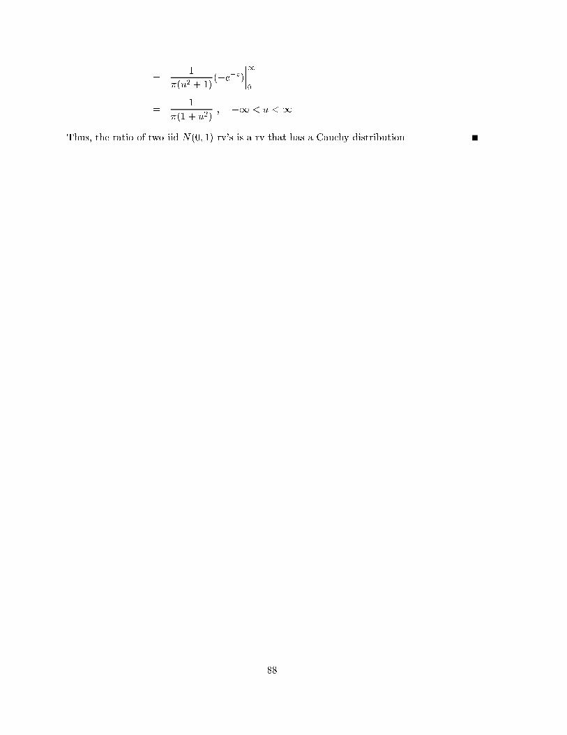
=1

�(u2 + 1)(�e�z)

����1

0

=1

�(1 + u2); �1 < u <1

Thus, the ratio of two iid N(0; 1) rv's is a rv that has a Cauchy distribution.

88

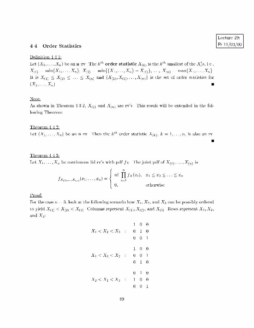
Lecture 29:

Fr 11/03/004.4 Order Statistics

De�nition 4.4.1:

Let (X1; : : : ;Xn) be an n{rv. The kth order statistic X(k) is the k

th smallest of the X 0is, i.e.,

X(1) = minfX1; : : : ;Xng, X(2) = minffX1; : : : ;Xng � X(1)g, : : :, X(n) = maxfX1; : : : ;Xng.It is X(1) � X(2) � : : : � X(n) and fX(1);X(2); : : : ; X(n)g is the set of order statistics for

(X1; : : : ; Xn).

Note:

As shown in Theorem 4.3.2, X(1) and X(n) are rv's. This result will be extended in the fol-

lowing Theorem:

Theorem 4.4.2:

Let (X1; : : : ; Xn) be an n{rv. Then the kth order statistic X(k), k = 1; : : : ; n, is also an rv.

Theorem 4.4.3:

Let X1; : : : ; Xn be continuous iid rv's with pdf fX . The joint pdf of X(1); : : : ;X(n) is

fX(1);:::;X(n)(x1; : : : ; xn) =

8>><>>:

n!nYi=1

fX(xi); x1 � x2 � : : : � xn

0; otherwise

Proof:

For the case n = 3, look at the following scenario how X1; X2, and X3 can be possibly ordered

to yield X(1) < X(2) < X(3). Columns represent X(1);X(2), and X(3). Rows represent X1;X2,

and X3:

X1 < X2 < X3 :

��������1 0 0

0 1 0

0 0 1

��������

X1 < X3 < X2 :

��������1 0 0

0 0 1

0 1 0

��������

X2 < X1 < X3 :

��������0 1 0

1 0 0

0 0 1

��������89

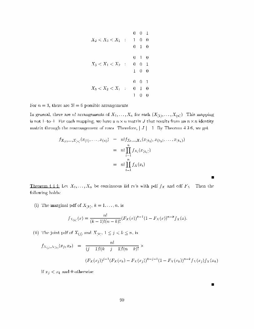
X2 < X3 < X1 :

��������0 0 1

1 0 0

0 1 0

��������

X3 < X1 < X2 :

��������0 1 0

0 0 1

1 0 0

��������

X3 < X2 < X1 :

��������0 0 1

0 1 0

1 0 0

��������For n = 3, there are 3! = 6 possible arrangements.

In general, there are n! arrangements of X1; : : : ;Xn for each (X(1); : : : ;X(n)). This mapping

is not 1{to{1. For each mapping, we have a n�n matrix J that results from an n�n identity

matrix through the rearrangement of rows. Therefore, j J j= 1. By Theorem 4.3.6, we get

fX(1);:::;X(n)(x(1); : : : ; x(n)) = n!fX1;:::;Xn(x(k1); x(k2); : : : ; x(kn))

= n!nYi=1

fXi(x(ki))

= n!nYi=1

fX(xi)

Theorem 4.4.4: Let X1; : : : ; Xn be continuous iid rv's with pdf fX and cdf FX . Then the

following holds:

(i) The marginal pdf of X(k), k = 1; : : : ; n, is

fX(k)(x) =

n!

(k � 1)!(n � k)!(FX(x))

k�1(1� FX(x))n�k

fX(x):

(ii) The joint pdf of X(j) and X(k), 1 � j < k � n, is

fX(j);X(k)(xj ; xk) =

n!

(j � 1)!(k � j � 1)!(n� k)!�

(FX(xj))j�1(FX(xk)� FX(xj))

k�j�1(1� FX(xk))n�k

fX(xj)fX(xk)

if xj < xk and 0 otherwise.

90

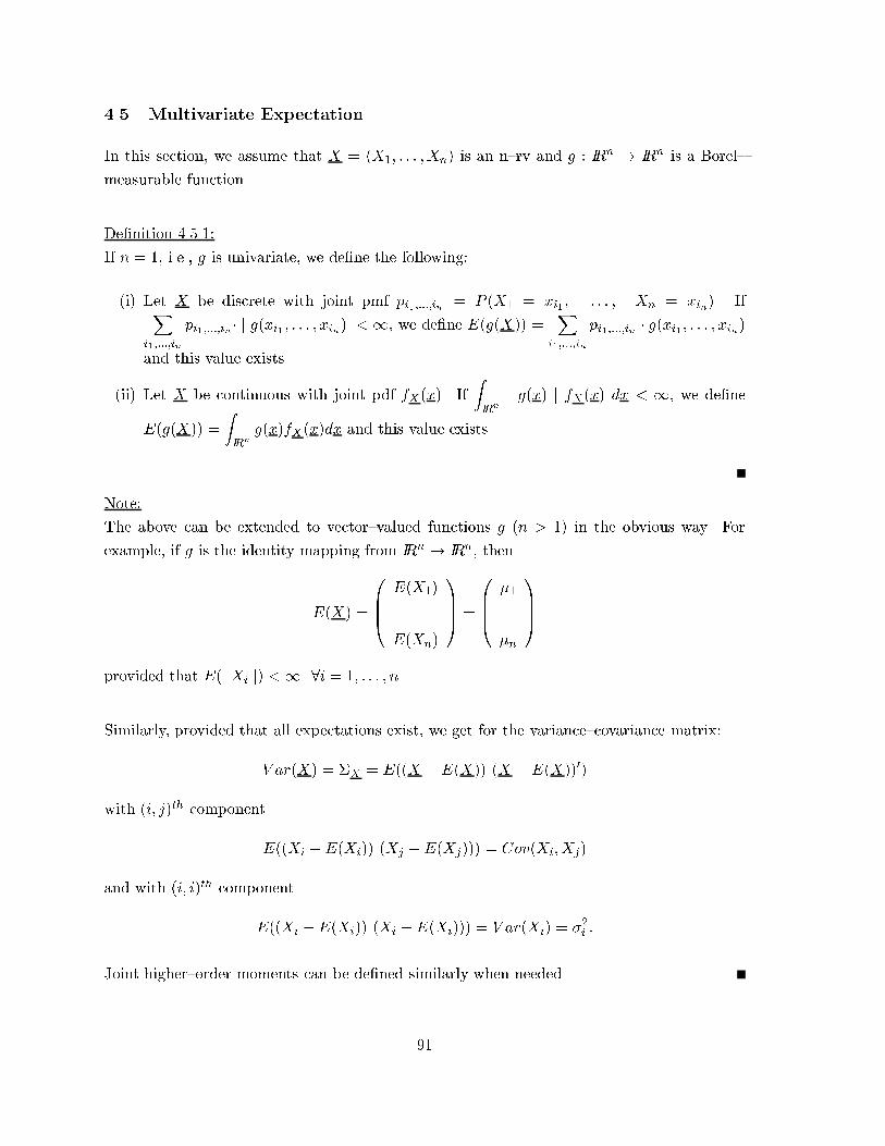
4.5 Multivariate Expectation

In this section, we assume that X = (X1; : : : ;Xn) is an n{rv and g : IRn ! IRn is a Borel{

measurable function.

De�nition 4.5.1:

If n = 1, i.e., g is univariate, we de�ne the following:

(i) Let X be discrete with joint pmf pi1;:::;in = P (X1 = xi1 ; : : : ; Xn = xin). IfXi1;:::;in

pi1;:::;in � j g(xi1 ; : : : ; xin) j<1, we de�ne E(g(X)) =X

i1;:::;in

pi1;:::;in � g(xi1 ; : : : ; xin)

and this value exists.

(ii) Let X be continuous with joint pdf fX(x). If

ZIRn

j g(x) j fX(x) dx < 1, we de�ne

E(g(X)) =

ZIRn

g(x)fX(x)dx and this value exists.

Note:

The above can be extended to vector{valued functions g (n > 1) in the obvious way. For

example, if g is the identity mapping from IRn ! IR

n, then

E(X) =

0BB@

E(X1)...

E(Xn)

1CCA =

0BB@

�1

...

�n

1CCA

provided that E(j Xi j) <1 8i = 1; : : : ; n.

Similarly, provided that all expectations exist, we get for the variance{covariance matrix:

V ar(X) = �X = E((X �E(X)) (X �E(X))0)

with (i; j)th component

E((Xi �E(Xi)) (Xj �E(Xj))) = Cov(Xi; Xj)

and with (i; i)th component

E((Xi �E(Xi)) (Xi �E(Xi))) = V ar(Xi) = �2i :

Joint higher{order moments can be de�ned similarly when needed.

91

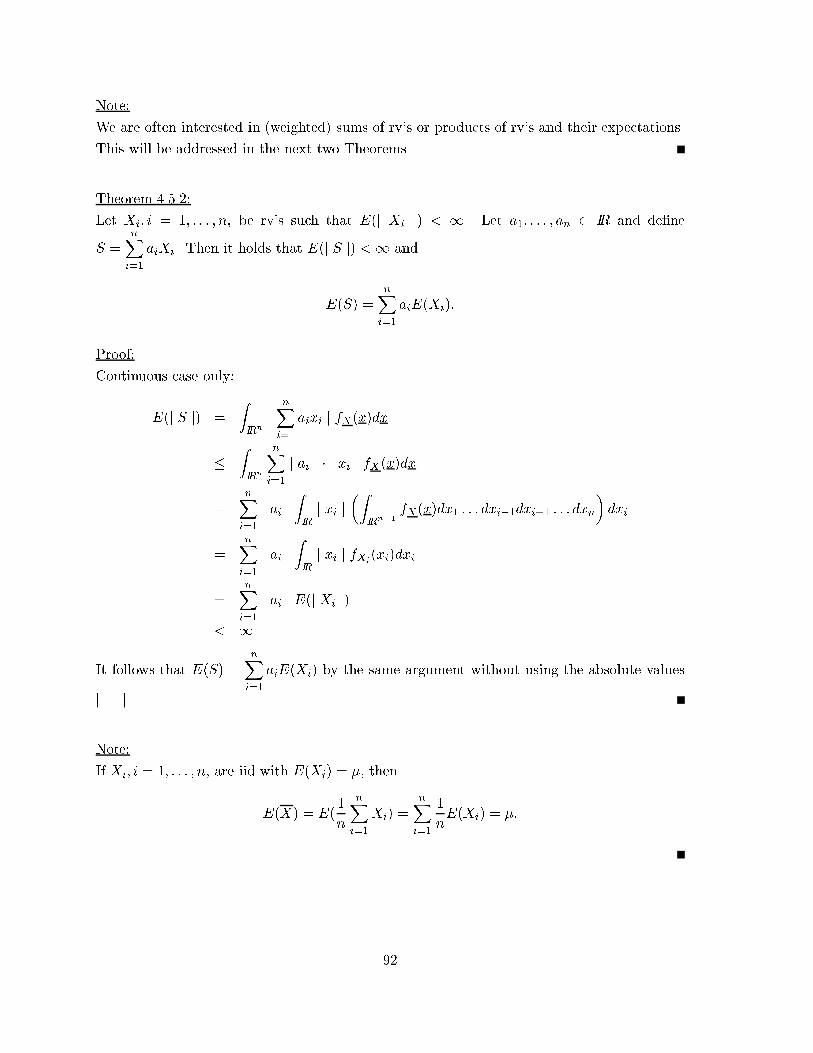
Note:

We are often interested in (weighted) sums of rv's or products of rv's and their expectations.

This will be addressed in the next two Theorems.

Theorem 4.5.2:

Let Xi; i = 1; : : : ; n, be rv's such that E(j Xi j) < 1. Let a1; : : : ; an 2 IR and de�ne

S =nXi=1

aiXi. Then it holds that E(j S j) <1 and

E(S) =nXi=1

aiE(Xi):

Proof:

Continuous case only:

E(j S j) =

ZIRn

jnXi=1

aixi j fX(x)dx

�ZIRn

nXi=1

j ai j � j xi j fX(x)dx

=nXi=1

j ai jZIRj xi j

�ZIRn�1

fX(x)dx1 : : : dxi�1dxi+1 : : : dxn

�dxi

=nXi=1

j ai jZIRj xi j fXi

(xi)dxi

=nXi=1

j ai j E(j Xi j)

< 1

It follows that E(S) =nXi=1

aiE(Xi) by the same argument without using the absolute values

j j.

Note:

If Xi; i = 1; : : : ; n, are iid with E(Xi) = �, then

E(X) = E(1

n

nXi=1

Xi) =nXi=1

1

nE(Xi) = �:

92

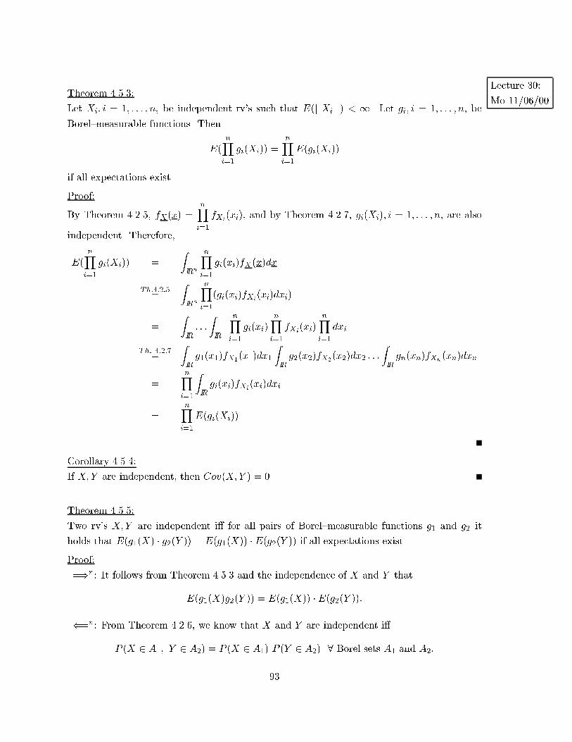
Lecture 30:

Mo 11/06/00Theorem 4.5.3:

Let Xi; i = 1; : : : ; n, be independent rv's such that E(j Xi j) < 1. Let gi; i = 1; : : : ; n, be

Borel{measurable functions. Then

E(nYi=1

gi(Xi)) =nYi=1

E(gi(Xi))

if all expectations exist.

Proof:

By Theorem 4.2.5, fX(x) =nYi=1

fXi(xi), and by Theorem 4.2.7, gi(Xi); i = 1; : : : ; n, are also

independent. Therefore,

E(nYi=1

gi(Xi)) =

ZIRn

nYi=1

gi(xi)fX(x)dx

Th:4:2:5=

ZIRn

nYi=1

(gi(xi)fXi(xi)dxi)

=

ZIR: : :

ZIR

nYi=1

gi(xi)nYi=1

fXi(xi)

nYi=1

dxi

Th: 4:2:7=

ZIRg1(x1)fX1

(x1)dx1

ZIRg2(x2)fX2

(x2)dx2 : : :

ZIRgn(xn)fXn(xn)dxn

=nYi=1

ZIRgi(xi)fXi

(xi)dxi

=nYi=1

E(gi(Xi))

Corollary 4.5.4:

If X;Y are independent, then Cov(X;Y ) = 0.

Theorem 4.5.5:

Two rv's X;Y are independent i� for all pairs of Borel{measurable functions g1 and g2 it

holds that E(g1(X) � g2(Y )) = E(g1(X)) � E(g2(Y )) if all expectations exist.

Proof:

\=)": It follows from Theorem 4.5.3 and the independence of X and Y that

E(g1(X)g2(Y )) = E(g1(X)) �E(g2(Y )):

\(=": From Theorem 4.2.6, we know that X and Y are independent i�

P (X 2 A1; Y 2 A2) = P (X 2 A1) P (Y 2 A2) 8 Borel sets A1 and A2:

93

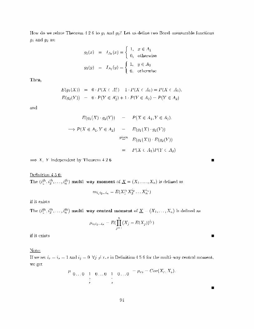
How do we relate Theorem 4.2.6 to g1 and g2? Let us de�ne two Borel{measurable functions

g1 and g2 as:

g1(x) = IA1(x) =

(1; x 2 A1

0; otherwise

g2(y) = IA2(y) =

(1; y 2 A2

0; otherwise

Then,

E(g1(X)) = 0 � P (X 2 Ac1) + 1 � P (X 2 A1) = P (X 2 A1);

E(g2(Y )) = 0 � P (Y 2 Ac2) + 1 � P (Y 2 A2) = P (Y 2 A2)

and

E(g1(X) � g2(Y )) = P (X 2 A1; Y 2 A2):

=) P (X 2 A1; Y 2 A2) = E(g1(X) � g2(Y ))given= E(g1(X)) �E(g2(Y ))

= P (X 2 A1)P (Y 2 A2)

=) X; Y independent by Theorem 4.2.6.

De�nition 4.5.6:

The (ith1 ; ith2 ; : : : ; i

thn ) multi{way moment of X = (X1; : : : ; Xn) is de�ned as

mi1i2:::in = E(Xi11 X

i22 : : : X

inn )

if it exists.

The (ith1 ; ith2 ; : : : ; i

thn ) multi{way central moment of X = (X1; : : : ;Xn) is de�ned as

�i1i2:::in = E(nYj=1

(Xj �E(Xj))ij )

if it exists.

Note:

If we set ir = is = 1 and ij = 0 8j 6= r; s in De�nition 4.5.6 for the multi{way central moment,

we get

�0 : : : 0 1 0 : : : 0 1 0 : : : 0

"r

"s

= �rs = Cov(Xr;Xs):

94

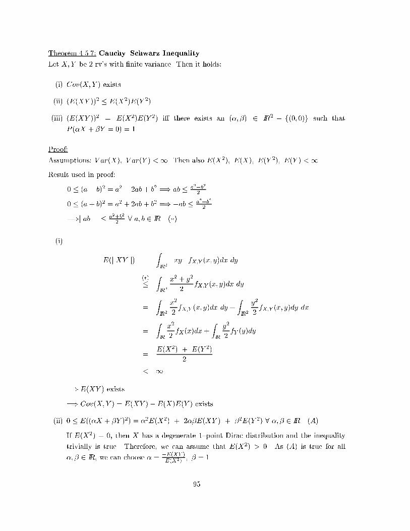
Theorem 4.5.7: Cauchy{Schwarz Inequality

Let X;Y be 2 rv's with �nite variance. Then it holds:

(i) Cov(X;Y ) exists.

(ii) (E(XY ))2 � E(X2)E(Y 2).

(iii) (E(XY ))2 = E(X2)E(Y 2) i� there exists an (�; �) 2 IR2 � f(0; 0)g such that

P (�X + �Y = 0) = 1.

Proof:

Assumptions: V ar(X); V ar(Y ) <1. Then also E(X2); E(X); E(Y 2); E(Y ) <1.

Result used in proof:

0 � (a� b)2 = a2 � 2ab+ b

2 =) ab � a2+b2

2

0 � (a+ b)2 = a2 + 2ab+ b

2 =) �ab � a2+b2

2

=)j ab j � a2+b2

2 8 a; b 2 IR (�)

(i)

E(j XY j) =

ZIR2

j xy j fX;Y (x; y)dx dy

(�)�

ZIR2

x2 + y

2

2fX;Y (x; y)dx dy

=

ZIR2

x2

2fX;Y (x; y)dx dy +

ZIR2

y2

2fX;Y (x; y)dy dx

=

ZIR

x2

2fX(x)dx+

ZIR

y2

2fY (y)dy

=E(X2) + E(Y 2)

2

< 1

=) E(XY ) exists

=) Cov(X;Y ) = E(XY )�E(X)E(Y ) exists

(ii) 0 � E((�X + �Y )2) = �2E(X2) + 2��E(XY ) + �

2E(Y 2) 8 �; � 2 IR (A)

If E(X2) = 0, then X has a degenerate 1{point Dirac distribution and the inequality

trivially is true. Therefore, we can assume that E(X2) > 0. As (A) is true for all

�; � 2 IR, we can choose � =�E(XY )E(X2)

; � = 1.

95

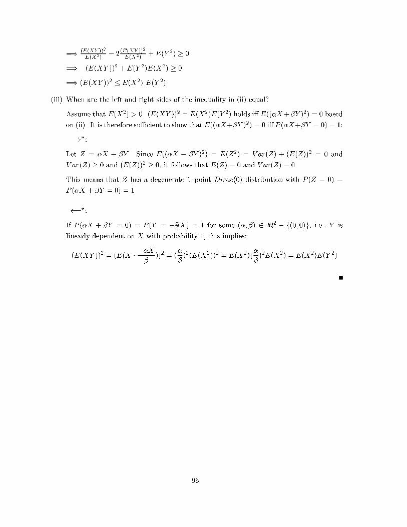
=) (E(XY ))2

E(X2)� 2

(E(XY ))2

E(X2)+E(Y 2) � 0

=) �(E(XY ))2 +E(Y 2)E(X2) � 0

=) (E(XY ))2 � E(X2) E(Y 2)

(iii) When are the left and right sides of the inequality in (ii) equal?

Assume that E(X2) > 0. (E(XY ))2 = E(X2)E(Y 2) holds i� E((�X+�Y )2) = 0 based

on (ii). It is therefore su�cient to show that E((�X+�Y )2) = 0 i� P (�X+�Y = 0) = 1:

\=)":

Let Z = �X + �Y . Since E((�X + �Y )2) = E(Z2) = V ar(Z) + (E(Z))2 = 0 and

V ar(Z) � 0 and (E(Z))2 � 0, it follows that E(Z) = 0 and V ar(Z) = 0.

This means that Z has a degenerate 1{point Dirac(0) distribution with P (Z = 0) =

P (�X + �Y = 0) = 1.

\(=":

If P (�X + �Y = 0) = P (Y = ���X) = 1 for some (�; �) 2 IR

2 � f(0; 0)g, i.e., Y is

linearly dependent on X with probability 1, this implies:

(E(XY ))2 = (E(X � ��X�

))2 = (�

�)2(E(X2))2 = E(X2)(

�

�)2E(X2) = E(X2)E(Y 2)

96

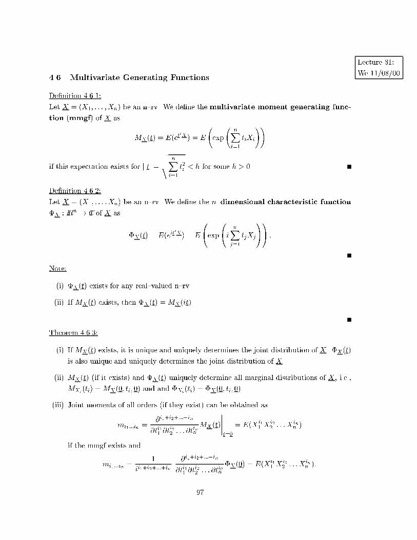
Lecture 31:

We 11/08/004.6 Multivariate Generating Functions

De�nition 4.6.1:

Let X = (X1; : : : ;Xn) be an n{rv. We de�ne the multivariate moment generating func-

tion (mmgf) of X as

MX(t) = E(et0X) = E

exp

nXi=1

tiXi

!!

if this expectation exists for j t j=

vuut nXi=1

t2i < h for some h > 0.

De�nition 4.6.2:

Let X = (X1; : : : ;Xn) be an n{rv. We de�ne the n{dimensional characteristic function

�X : IRn ! CI of X as

�X(t) = E(eit0X) = E

0@exp

0@i nX

j=1

tjXj

1A1A :

Note:

(i) �X(t) exists for any real{valued n{rv.

(ii) If MX(t) exists, then �X(t) =MX(it).

Theorem 4.6.3:

(i) If MX(t) exists, it is unique and uniquely determines the joint distribution of X . �X(t)

is also unique and uniquely determines the joint distribution of X .

(ii) MX(t) (if it exists) and �X(t) uniquely determine all marginal distributions of X, i.e.,

MXi(ti) =MX(0; ti; 0) and and �Xi

(ti) = �X(0; ti; 0).

(iii) Joint moments of all orders (if they exist) can be obtained as

mi1:::in =@i1+i2+:::+in

@ti11 @t

i22 : : : @t

inn

MX(t)

�����t=0

= E(Xi11 X

i22 : : : X

inn )

if the mmgf exists and

mi1:::in =1

ii1+i2+:::+in

@i1+i2+:::+in

@ti11 @t

i22 : : : @t

inn

�X(0) = E(Xi11 X

i22 : : : X

inn ):

97

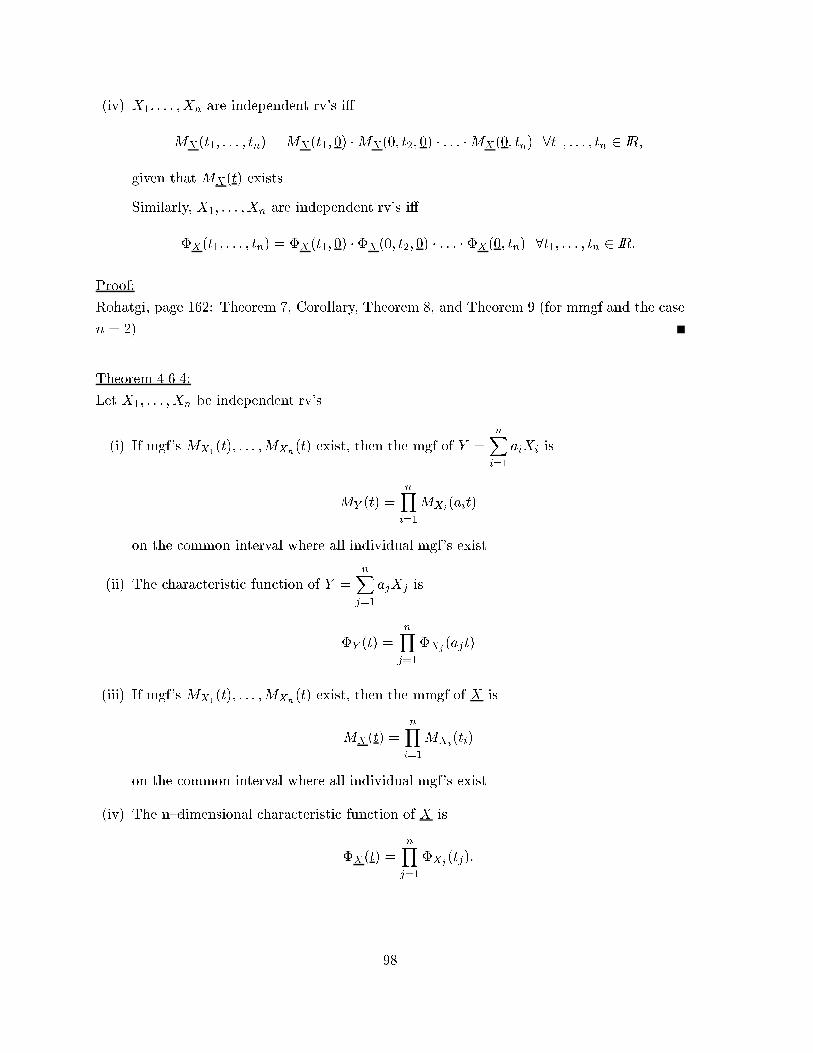
(iv) X1; : : : ;Xn are independent rv's i�

MX(t1; : : : ; tn) =MX(t1; 0) �MX(0; t2; 0) � : : : �MX(0; tn) 8t1; : : : ; tn 2 IR;

given that MX(t) exists.

Similarly, X1; : : : ;Xn are independent rv's i�

�X(t1; : : : ; tn) = �X(t1; 0) � �X(0; t2; 0) � : : : � �X(0; tn) 8t1; : : : ; tn 2 IR:

Proof:

Rohatgi, page 162: Theorem 7, Corollary, Theorem 8, and Theorem 9 (for mmgf and the case

n = 2).

Theorem 4.6.4:

Let X1; : : : ; Xn be independent rv's.

(i) If mgf's MX1(t); : : : ;MXn(t) exist, then the mgf of Y =

nXi=1

aiXi is

MY (t) =nYi=1

MXi(ait)

on the common interval where all individual mgf's exist.

(ii) The characteristic function of Y =nXj=1

ajXj is

�Y (t) =nYj=1

�Xj(ajt)

(iii) If mgf's MX1(t); : : : ;MXn(t) exist, then the mmgf of X is

MX(t) =nYi=1

MXi(ti)

on the common interval where all individual mgf's exist.

(iv) The n{dimensional characteristic function of X is

�X(t) =nYj=1

�Xj(tj):

98

Proof:

Homework (parts (ii) and (iv) only)

Theorem 4.6.5:

LetX1; : : : ; Xn be independent discrete rv's on the non{negative integers with pgf'sGX1(s); : : : ; GXn(s).

The pgf of Y =nXi=1

Xi is

GY (s) =nYi=1

GXi(s):

Proof:

Version 1:

GXi(s) = E(sXi)

GY (s) = E(sY )

= E(sPn

i=1Xi)

indep:=

nYi=1

E(sXi)

=nYi=1

GXi(s)

Version 2: (case n = 2 only)

GY (s) = P (Y = 0) + P (Y = 1)s+ P (Y = 2)s2 + : : :

= P (X1 = 0; X2 = 0) +

(P (X1 = 1;X2 = 0) + P (X1 = 0;X2 = 1)) s+

(P (X1 = 2;X2 = 0) + P (X1 = 1;X2 = 1) + P (X1 = 0;X2 = 2)) s2 + : : :

indep:= P (X1 = 0)P (X2 = 0) +

(P (X1 = 1)P (X2 = 0) + P (X1 = 0)P (X2 = 1)) s+

(P (X1 = 2)P (X2 = 0) + P (X1 = 1)P (X2 = 1) + P (X1 = 0)P (X2 = 2)) s2 + : : :

=�P (X1 = 0) + P (X1 = 1)s+ P (X1 = 2)s2 + : : :

���

P (X2 = 0) + P (X2 = 1)s+ P (X2 = 2)s2 + : : :

�= GX1

(s) �GX2(s)

A generalized proof for n � 3 needs to be done by induction on n.

99

Theorem 4.6.6:

Let X1; : : : ;XN be iid discrete rv's on the non{negative integers with common pgf GX(s).

Let N be a discrete rv on the non{negative integers with pgf GN(s). Let N be independent

of the Xi's. De�ne SN =NXi=1

Xi. The pgf of SN is

GSN (s) = GN (GX(s)):

Proof:

P (SN = k) =1Xn=0

P (SN = kjN = n) � P (N = n)

=) GSN (s) =1Xk=0

1Xn=0

P (SN = kjN = n) � P (N = n) � sk

=1Xn=0

P (N = n)1Xk=0

P (SN = kjN = n) � sk

=1Xn=0

P (N = n)1Xk=0

P (Sn = k) � sk

=1Xn=0

P (N = n)1Xk=0

P (nXi=1

Xi = k) � sk

Th:4:6:5=

1Xn=0

P (N = n)nYi=1

GXi(s)

iid=

1Xn=0

P (N = n) � (GX(s))n

= GN (GX(s))

Example 4.6.7:

Starting with a single cell at time 0, after one time unit there is probability p that the cell will

have split (2 cells), probability q that it will survive without splitting (1 cell), and probability

r that it will have died (0 cells). It holds that p; q; r � 0 and p + q + r = 1. Any surviving

cells have the same probabilities of splitting or dying. What is the pgf for the # of cells at

time 2?

GX(s) = GN (s) = ps2 + qs+ r

GSN (s) = p(ps2 + ps+ r)2 + q(ps2 + ps+ r) + r

100

Theorem 4.6.8:

Let X1; : : : ;XN be iid rv's with common mgf MX(t). Let N be a discrete rv on the non{

negative integers with mgf MN (t). Let N be independent of the Xi's. De�ne SN =NXi=1

Xi.

The mgf of SN is

MSN (t) =MN (lnMX(t)):

Proof:

Consider the case that the Xi's are non{negative integers:

We know that

GX(s) = E(sX) = E(eln sX

) = E(e(ln s)�X) =MX(ln s)

=)MX(s) = GX(es)

=)MSN (t) = GSN (et)

Th:4:6:6= GN (GX(e

t)) = GN (MX(t)) =MN (lnMX(t))

In the general case, i.e., if the X 0is are not non{negative integers, we need results from Section

4.7 (conditional expectation) to proof this Theorem.

101

Lecture 32:

Fr 11/10/004.7 Conditional Expectation

In Section 4.1, we established that the conditional pmf of X given Y = yj (for PY (yj) > 0)

is a pmf. For continuous rv's X and Y , when fY (y) > 0, fXjY (x j y) =fX;Y (x;y)

fY (y), and fX;Y

and fY are continuous, then fXjY (x j y) is a pdf and it is the conditional pdf of X given Y = y.

De�nition 4.7.1:

Let X;Y be rv's on (; L; P ). Let h be a Borel{measurable function. Assume that E(h(X))

exists. Then the conditional expectation of h(X) given Y , i.e., E(h(X) j Y ), is a rv that

takes the value E(h(X) j y). It is de�ned as

E(h(X) j y) =

8>>>><>>>>:

Xx2X

h(x)P (X = x j Y = y); if (X;Y ) is discrete and P (Y = y) > 0

Z 1

�1h(x)fXjY (x j y)dx; if (X;Y ) is continuous and fY (y) > 0

Note:

(i) The rv E(h(X) j Y ) = g(Y ) is a function of Y as a rv.

(ii) The usual properties of expectations apply to the conditional expectation:

(a) E(c j Y ) = c 8c 2 IR.

(b) E(aX + b j Y ) = aE(X j Y ) + b 8a; b 2 IR.

(c) If g1; g2 are Borel{measurable functions and if E(g1(X)); E(g2(X)) exist, then

E(a1g1(X) + a2g2(X) j Y ) = a1E(g1(X) j Y ) + a2E(g2(X) j Y ) 8a1; a2 2 IR.

(d) If X � 0 then E(X j Y ) � 0.

(e) If X1 � X2 then E(X1 j Y ) � E(X2 j Y ).

(iii) Moments are de�ned in the usual way. If E(j X jr) <1, then E(Xr j Y ) exists and is

the rth conditional moment of X given Y .

102

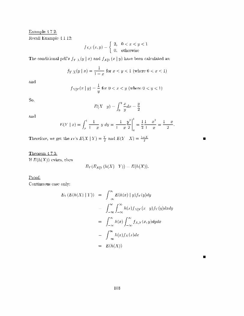
Example 4.7.2:

Recall Example 4.1.12:

fX;Y (x; y) =

(2; 0 < x < y < 1

0; otherwise

The conditional pdf's fY jX(y j x) and fXjY (x j y) have been calculated as:

fY jX(y j x) =1

1� xfor x < y < 1 (where 0 < x < 1)

and

fXjY (x j y) =1

yfor 0 < x < y (where 0 < y < 1).

So,

E(X j y) =Z y

0

x

ydx =

y

2

and

E(Y j x) =Z 1

x

1

1� xy dy =

1

1� x

y2

2

�����1

x

=1

2

1� x2

1� x=

1 + x

2:

Therefore, we get the rv's E(X j Y ) = Y2 and E(Y j X) = 1+X

2 .

Theorem 4.7.3:

If E(h(X)) exists, then

EY (EXjY (h(X) j Y )) = E(h(X)):

Proof:

Continuous case only:

EY (E(h(X) j Y )) =

Z 1

�1E(h(x) j y)fY (y)dy

=

Z 1

�1

Z 1

�1h(x)fXjY (x j y)fY (y)dxdy

=

Z 1

�1h(x)

Z 1

�1fX;Y (x; y)dydx

=

Z 1

�1h(x)fX(x)dx

= E(h(X))

103

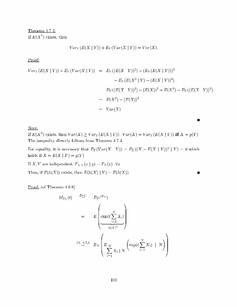
Theorem 4.7.4:

If E(X2) exists, then

V arY (E(X j Y )) +EY (V ar(X j Y )) = V ar(X):

Proof:

V arY (E(X j Y )) +EY (V ar(X j Y )) = EY ((E(X j Y ))2)� (EY (E(X j Y )))2

+EY (E(X2 j Y )� (E(X j Y ))2)

= EY ((E(X j Y ))2)� (E(X))2 +E(X2)�EY ((E(X j Y ))2)

= E(X2)� (E(X))2

= V ar(X)

Note:

If E(X2) exists, then V ar(X) � V arY (E(X j Y )). V ar(X) = V arY (E(X j Y )) i� X = g(Y ).

The inequality directly follows from Theorem 4.7.4.

For equality, it is necessary that EY (V ar(X j Y )) = EY ((X � E(X j Y ))2 j Y ) = 0 which

holds if X = E(X j Y ) = g(Y ).

If X;Y are independent, FXjY (x j y) = FX(x) 8x.

Thus, if E(h(X)) exists, then E(h(X) j Y ) = E(h(X)).

Proof: (of Theorem 4.6.8)

MSN (t)Def:= E(etSN )

= E

0BBBBB@exp(t

NXi=1

Xi)

| {z }\h(X)00

1CCCCCA

Th: 4:7:3= EN

0BBBB@E NX

i=1

Xi j N

exp(t

NXi=1

Xi) j N!1CCCCA

104

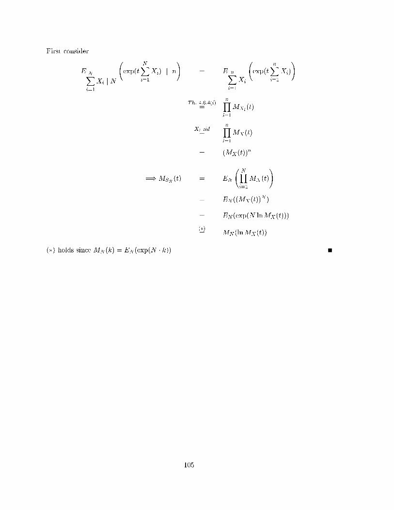
First consider

E NXi=1

Xi j N

exp(t

NXi=1

Xi) j n!

= E nXi=1

Xi

exp(t

nXi=1

Xi)

!

Th: 4:6:4(i)=

nYi=1

MXi(t)

Xi iid=

nYi=1

MX(t)

= (MX(t))n

=)MSN (t) = EN

NYi=1

MX(t)

!

= EN ((MX (t))N )

= EN (exp(N lnMX(t)))

(�)= MN (lnMX(t))

(�) holds since MN (k) = EN (exp(N � k)).

105

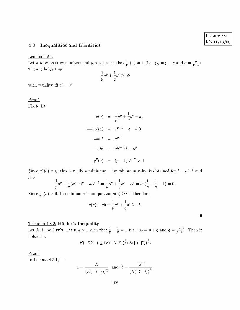
Lecture 33:

Mo 11/13/004.8 Inequalities and Identities

Lemma 4.8.1:

Let a; b be positive numbers and p; q > 1 such that 1p +

1q = 1 (i.e., pq = p+ q and q = p

p�1).

Then it holds that1

pap +

1

qbq � ab

with equality i� ap = b

q.

Proof:

Fix b. Let

g(a) =1

pap +

1

qbq � ab

=) g0(a) = a

p�1 � b!= 0

=) b = ap�1

=) bq = a

(p�1)q = ap

g00(a) = (p� 1)ap�2 > 0

Since g00(a) > 0, this is really a minimum. The minimum value is obtained for b = ap�1 and

it is1

pap +

1

q(ap�1)q � aa

p�1 =1

pap +

1

qap � a

p = ap(1

p+1

q� 1) = 0:

Since g00(a) > 0, the minimum is unique and g(a) � 0. Therefore,

g(a) + ab =1

pap +

1

qbq � ab:

Theorem 4.8.2: H�older's Inequality

Let X;Y be 2 rv's. Let p; q > 1 such that 1p +

1q = 1 (i.e., pq = p+ q and q = p

p�1). Then it

holds that

E(j XY j) � (E(j X jp))1p (E(j Y jq))

1q :

Proof:

In Lemma 4.8.1, let

a =j X j

(E(j X jp))1p

and b =j Y j

(E(j Y jq))1q

:

106

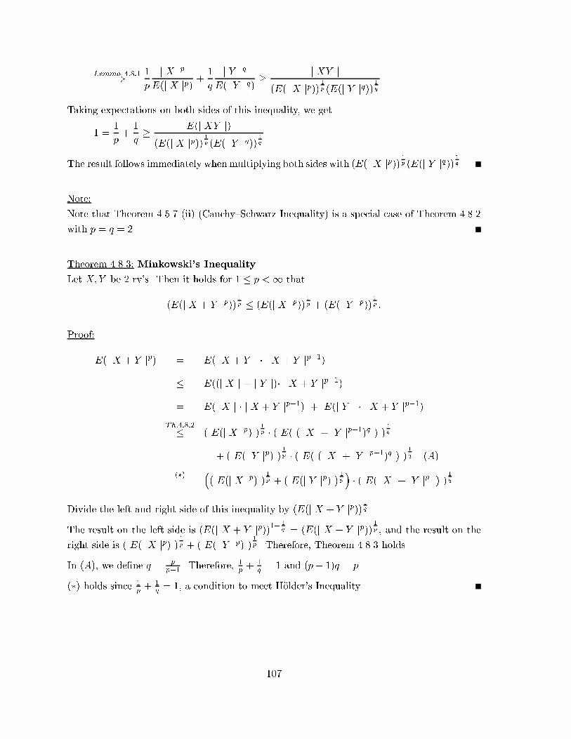
Lemma 4:8:1=) 1

p

j X jpE(j X jp) +

1

q

j Y jqE(j Y jq) �

j XY j(E(j X jp))

1p (E(j Y jq))

1q

Taking expectations on both sides of this inequality, we get

1 =1

p+1

q� E(j XY j)

(E(j X jp))1p (E(j Y jq))

1q

The result follows immediately when multiplying both sides with (E(j X jp))1p (E(j Y jq))

1q .

Note:

Note that Theorem 4.5.7 (ii) (Cauchy{Schwarz Inequality) is a special case of Theorem 4.8.2

with p = q = 2.

Theorem 4.8.3: Minkowski's Inequality

Let X;Y be 2 rv's. Then it holds for 1 � p <1 that

(E(j X + Y jp))1p � (E(j X jp))

1p + (E(j Y jp))

1p :

Proof:

E(j X + Y jp) = E(j X + Y j � j X + Y jp�1)

� E((j X j + j Y j)� j X + Y jp�1)

= E(j X j � j X + Y jp�1) + E(j Y j � j X + Y jp�1)Th:4:8:2� ( E(j X jp) )

1p � ( E( (j X + Y jp�1)q ) )

1q

+ ( E(j Y jp) )1p � ( E( (j X + Y jp�1)q ) )

1q (A)

(�)=

�( E(j X jp) )

1p + ( E(j Y jp) )

1p

�� ( E(j X + Y jp ) )

1q

Divide the left and right side of this inequality by (E(j X + Y jp))1q .

The result on the left side is (E(j X + Y jp))1�1q = (E(j X + Y jp))

1p , and the result on the

right side is ( E(j X jp) )1p + ( E(j Y jp) )

1p . Therefore, Theorem 4.8.3 holds.

In (A), we de�ne q = pp�1 . Therefore,

1p +

1q = 1 and (p� 1)q = p.

(�) holds since 1p +

1q = 1, a condition to meet H�older's Inequality.

107

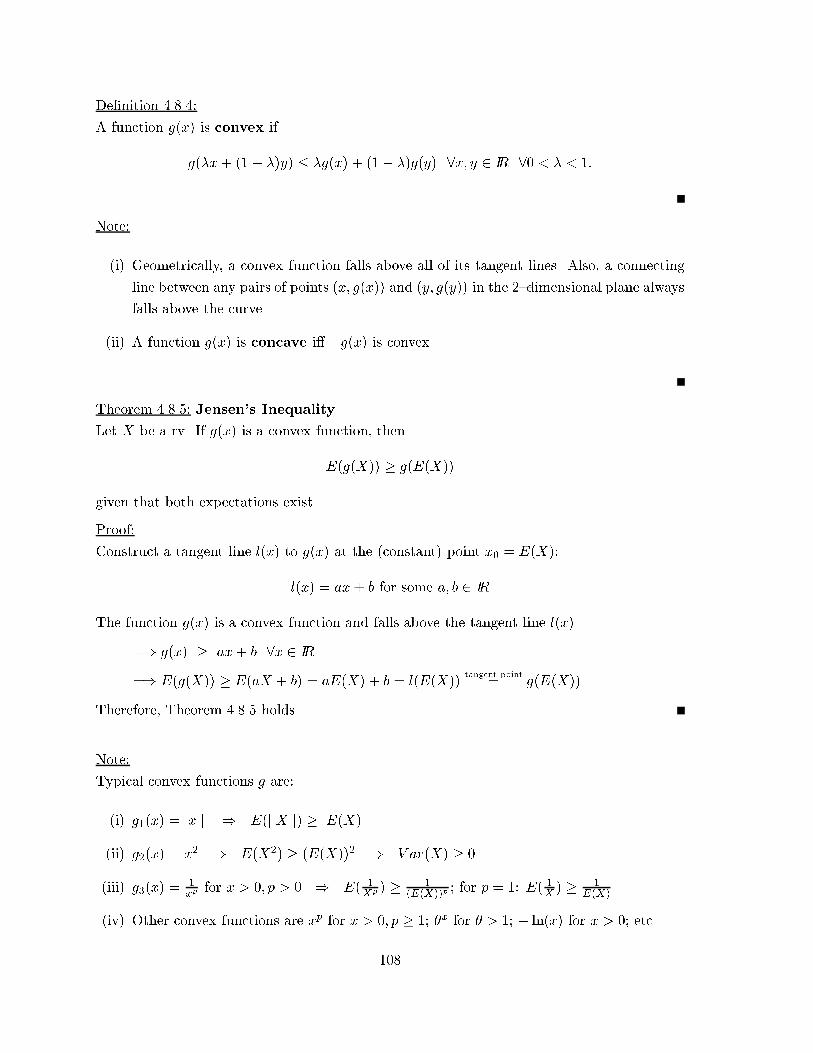
De�nition 4.8.4:

A function g(x) is convex if

g(�x+ (1� �)y) � �g(x) + (1� �)g(y) 8x; y 2 IR 80 < � < 1:

Note:

(i) Geometrically, a convex function falls above all of its tangent lines. Also, a connecting

line between any pairs of points (x; g(x)) and (y; g(y)) in the 2{dimensional plane always

falls above the curve.

(ii) A function g(x) is concave i� �g(x) is convex.

Theorem 4.8.5: Jensen's Inequality

Let X be a rv. If g(x) is a convex function, then

E(g(X)) � g(E(X))

given that both expectations exist.

Proof:

Construct a tangent line l(x) to g(x) at the (constant) point x0 = E(X):

l(x) = ax+ b for some a; b 2 IR

The function g(x) is a convex function and falls above the tangent line l(x)

=) g(x) � ax+ b 8x 2 IR

=) E(g(X)) � E(aX + b) = aE(X) + b = l(E(X))tangent point

= g(E(X))

Therefore, Theorem 4.8.5 holds.

Note:

Typical convex functions g are:

(i) g1(x) =j x j ) E(j X j) �j E(X) j.

(ii) g2(x) = x2 ) E(X2) � (E(X))2 ) V ar(X) � 0.

(iii) g3(x) =1xp for x > 0; p > 0 ) E( 1

Xp ) � 1(E(X))p ; for p = 1: E( 1X ) �

1E(X)

(iv) Other convex functions are xp for x > 0; p � 1; �x for � > 1; � ln(x) for x > 0; etc.

108

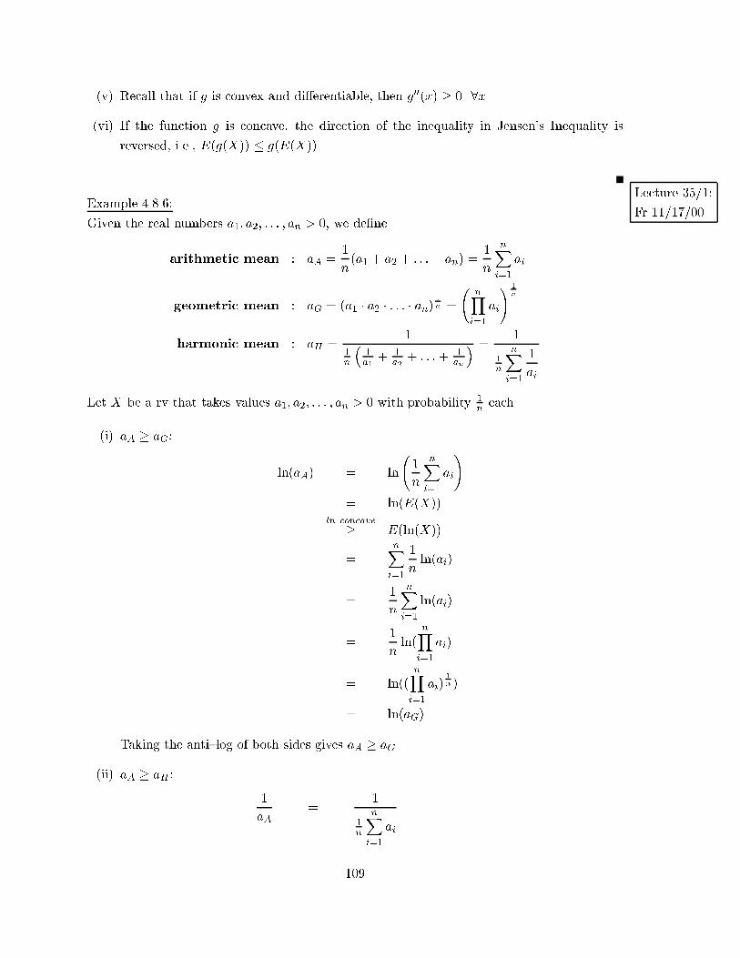
(v) Recall that if g is convex and di�erentiable, then g00(x) � 0 8x.

(vi) If the function g is concave, the direction of the inequality in Jensen's Inequality is

reversed, i.e., E(g(X)) � g(E(X)).

Lecture 35/1:

Fr 11/17/00Example 4.8.6:

Given the real numbers a1; a2; : : : ; an > 0, we de�ne

arithmetic mean : aA =1

n(a1 + a2 + : : : + an) =

1

n

nXi=1

ai

geometric mean : aG = (a1 � a2 � : : : � an)1n =

nYi=1

ai

! 1n

harmonic mean : aH =1

1n

�1a1+ 1

a2+ : : :+ 1

an

� =1

1n

nXi=1

1

ai

Let X be a rv that takes values a1; a2; : : : ; an > 0 with probability 1neach.

(i) aA � aG:

ln(aA) = ln

1

n

nXi=1

ai

!

= ln(E(X))

ln concave� E(ln(X))

=nXi=1

1

nln(ai)

=1

n

nXi=1

ln(ai)

=1

nln(

nYi=1

ai)

= ln((nYi=1

ai)1n )

= ln(aG)

Taking the anti{log of both sides gives aA � aG.

(ii) aA � aH :

1

aA=

1

1n

nXi=1

ai

109

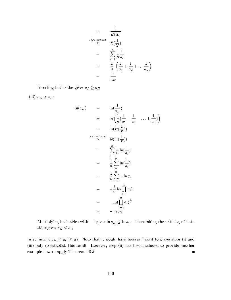
=1

E(X)

1=X convex

� E(1

X)

=nXi=1

1

n

1

ai

=1

n

�1

a1+

1

a2+ : : :

1

an

�

=1

aH

Inverting both sides gives aA � aH .

(iii) aG � aH :

� ln(aH) = ln(1

aH)

= ln

�1

n(1

a1+

1

a2+ : : :+

1

an)

�

= ln(E(1

X))

ln concave� E(ln(

1

X))

=nXi=1

1

nln(

1

ai)

=1

n

nXi=1

ln(1

ai)

=1

n

nXi=1

� lnai

= � 1

nln(

nYi=1

ai)

= � ln(nYi=1

ai)1n

= � lnaG

Multiplying both sides with �1 gives lnaH � lnaG. Then taking the anti{log of both

sides gives aH � aG.

In summary, aH � aG � aA. Note that it would have been su�cient to prove steps (i) and

(iii) only to establish this result. However, step (ii) has been included to provide another

example how to apply Theorem 4.8.5.

110

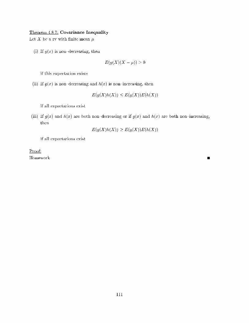
Theorem 4.8.7: Covariance Inequality

Let X be a rv with �nite mean �.

(i) If g(x) is non{decreasing, then

E(g(X)(X � �)) � 0

if this expectation exists.

(ii) If g(x) is non{decreasing and h(x) is non{increasing, then

E(g(X)h(X)) � E(g(X))E(h(X))

if all expectations exist.

(iii) If g(x) and h(x) are both non{decreasing or if g(x) and h(x) are both non{increasing,

then

E(g(X)h(X)) � E(g(X))E(h(X))

if all expectations exist.

Proof:

Homework

111

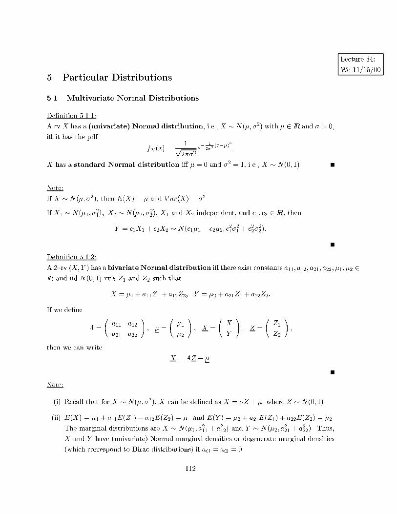
Lecture 34:

We 11/15/00

5 Particular Distributions

5.1 Multivariate Normal Distributions

De�nition 5.1.1:

A rv X has a (univariate) Normal distribution, i.e., X � N(�; �2) with � 2 IR and � > 0,

i� it has the pdf

fX(x) =1p2��2

e� 1

2�2(x��)2

:

X has a standard Normal distribution i� � = 0 and �2 = 1, i.e., X � N(0; 1).

Note:

If X � N(�; �2), then E(X) = � and V ar(X) = �2.

If X1 � N(�1; �21); X2 � N(�2; �

22), X1 and X2 independent, and c1; c2 2 IR, then

Y = c1X1 + c2X2 � N(c1�1 + c2�2; c21�

21 + c

22�

22):

De�nition 5.1.2:

A 2{rv (X;Y ) has a bivariate Normal distribution i� there exist constants a11; a12; a21; a22; �1; �2 2IR and iid N(0; 1) rv's Z1 and Z2 such that

X = �1 + a11Z1 + a12Z2; Y = �2 + a21Z1 + a22Z2:

If we de�ne

A =

a11 a12

a21 a22

!; � =

�1

�2

!; X =

X

Y

!; Z =

Z1

Z2

!;

then we can write

X = AZ + �:

Note:

(i) Recall that for X � N(�; �2), X can be de�ned as X = �Z + �, where Z � N(0; 1).

(ii) E(X) = �1 + a11E(Z1) + a12E(Z2) = �1 and E(Y ) = �2 + a21E(Z1) + a22E(Z2) = �2.

The marginal distributions are X � N(�1; a211 + a

212) and Y � N(�2; a

221 + a

222). Thus,

X and Y have (univariate) Normal marginal densities or degenerate marginal densities

(which correspond to Dirac distributions) if ai1 = ai2 = 0.

112

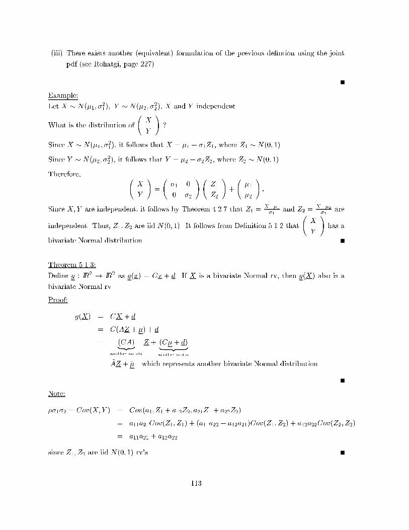
(iii) There exists another (equivalent) formulation of the previous de�ntion using the joint

pdf (see Rohatgi, page 227).

Example:

Let X � N(�1; �21); Y � N(�2; �

22), X and Y independent.

What is the distribution of

X

Y

!?

Since X � N(�1; �21), it follows that X = �1 + �1Z1, where Z1 � N(0; 1).

Since Y � N(�2; �22), it follows that Y = �2 + �2Z2, where Z2 � N(0; 1).

Therefore, X

Y

!=

�1 0

0 �2

! Z1

Z2

!+

�1

�2

!:

Since X;Y are independent, it follows by Theorem 4.2.7 that Z1 =X��1�1

and Z2 =X��2�2

are

independent. Thus, Z1; Z2 are iid N(0; 1). It follows from De�nition 5.1.2 that

X

Y

!has a

bivariate Normal distribution.

Theorem 5.1.3:

De�ne g : IR2 ! IR2 as g(x) = Cx + d. If X is a bivariate Normal rv, then g(X) also is a

bivariate Normal rv.

Proof:

g(X) = CX + d

= C(AZ + �) + d

= (CA)| {z }another matrix

Z + (C�+ d)| {z }another vector

= ~AZ + ~� which represents another bivariate Normal distribution

Note:

��1�2 = Cov(X;Y ) = Cov(a11Z1 + a12Z2; a21Z1 + a22Z2)

= a11a21Cov(Z1; Z1) + (a11a22 + a12a21)Cov(Z1; Z2) + a12a22Cov(Z2; Z2)

= a11a21 + a12a22

since Z1; Z2 are iid N(0; 1) rv's.

113

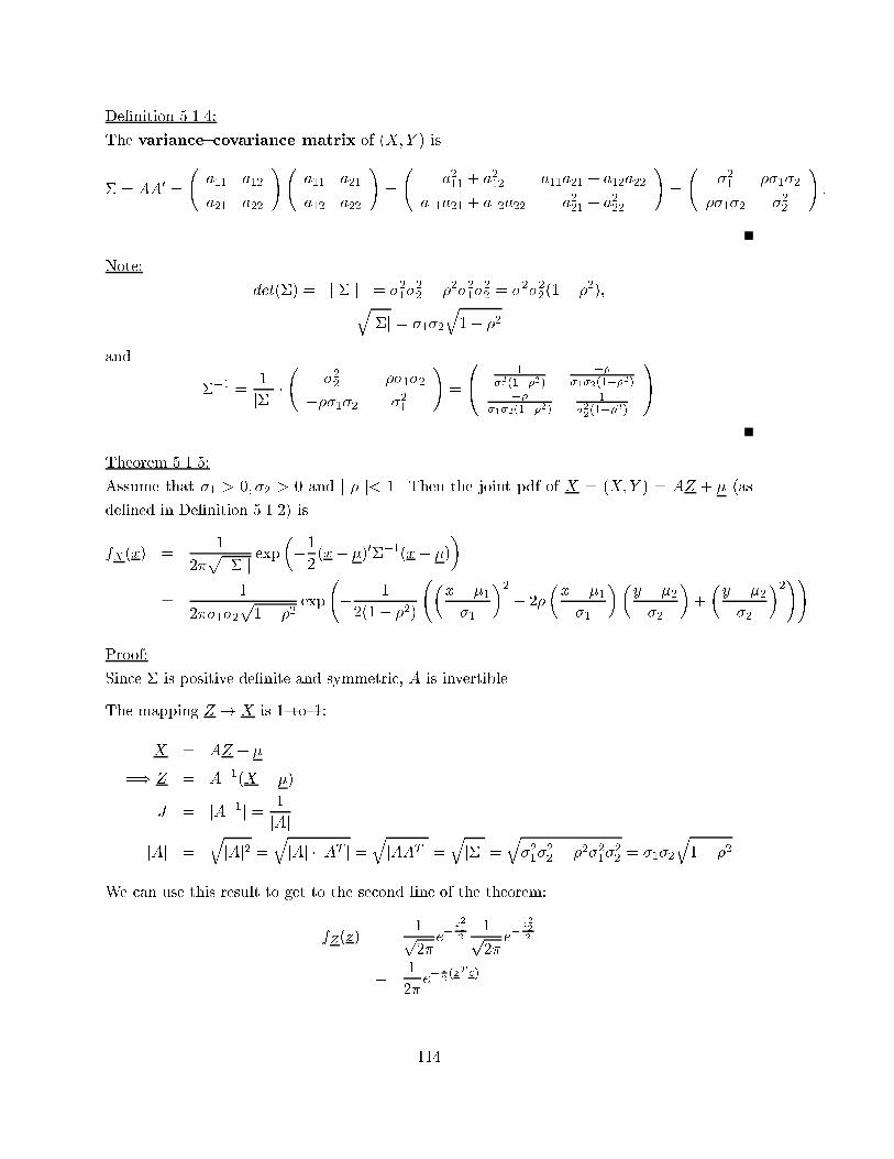
De�nition 5.1.4:

The variance{covariance matrix of (X;Y ) is

� = AA0 =

a11 a12

a21 a22

! a11 a21

a12 a22

!=

a211 + a

212 a11a21 + a12a22

a11a21 + a12a22 a221 + a

222

!=

�21 ��1�2

��1�2 �22

!:

Note:

det(�) = j � j = �21�

22 � �

2�21�

22 = �

21�

22(1� �

2);qj�j = �1�2

q1� �2

and

��1 =1

j�j �

�22 ���1�2

���1�2 �21

!=

0@ 1

�21(1��2)��

�1�2(1��2)��

�1�2(1��2)1

�22(1��2)

1A

Theorem 5.1.5:

Assume that �1 > 0; �2 > 0 and j � j< 1. Then the joint pdf of X = (X;Y ) = AZ + � (as

de�ned in De�nition 5.1.2) is

fX(x) =1

2�pj � j

exp

��1

2(x� �)0��1(x� �)

�

=1

2��1�2p1� �2

exp

� 1

2(1 � �2)

�x� �1

�1

�2� 2�

�x� �1

�1

��y � �2

�2

�+

�y � �2

�2

�2!!

Proof:

Since � is positive de�nite and symmetric, A is invertible.

The mapping Z ! X is 1{to{1:

X = AZ + �

=) Z = A�1(X � �)

J = jA�1j = 1

jAj

jAj =qjAj2 =

qjAj � jAT j =

qjAAT j =

qj�j =

q�21�

22 � �2�21�

22 = �1�2

q1� �2

We can use this result to get to the second line of the theorem:

fZ(z) =1p2�

e� z2

12

1p2�

e� z2

22

=1

2�e� 12(zT z)

114

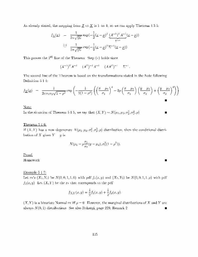
As already stated, the mapping from Z to X is 1{to{1, so we can apply Theorem 4.3.5:

fX(x) =1

2�pj�j

exp(�1

2(x� �)T (A�1)TA�1| {z }

��1

(x� �))

(�)=

1

2�pj�j

exp(�1

2(x� �)T��1(x� �))

This proves the 1st line of the Theorem. Step (�) holds since

(A�1)TA�1 = (AT )�1A�1 = (AAT )�1 = ��1:

The second line of the Theorem is based on the transformations stated in the Note following

De�nition 5.1.4:

fX(x) =1

2��1�2p1� �2

exp

� 1

2(1 � �2)

�x� �1

�1

�2� 2�

�x� �1

�1

��y � �2

�2

�+

�y � �2

�2

�2!!

Note:

In the situation of Theorem 5.1.5, we say that (X;Y ) � N(�1; �2; �21 ; �

22 ; �).

Theorem 5.1.6:

If (X;Y ) has a non{degenerate N(�1; �2; �21 ; �

22 ; �) distribution, then the conditional distri-

bution of X given Y = y is

N(�1 + ��1

�2(y � �2); �

21(1� �

2)):

Proof:

Homework

Example 5.1.7:

Let rv's (X1; Y1) be N(0; 0; 1; 1; 0) with pdf f1(x; y) and (X2; Y2) be N(0; 0; 1; 1; �) with pdf

f2(x; y). Let (X;Y ) be the rv that corresponds to the pdf

fX;Y (x; y) =1

2f1(x; y) +

1

2f2(x; y):

(X;Y ) is a bivariate Normal rv i� � = 0. However, the marginal distributions of X and Y are

always N(0; 1) distributions. See also Rohatgi, page 229, Remark 2.

115

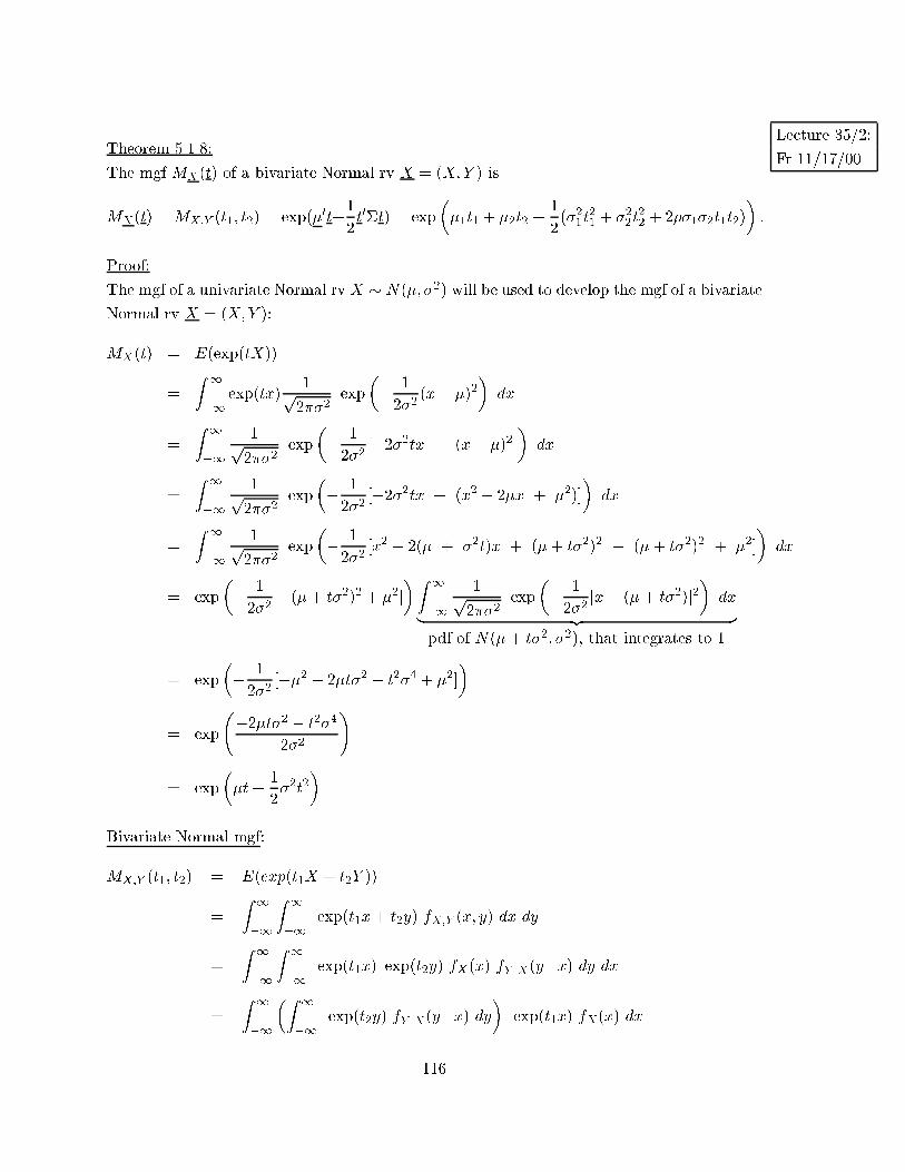
Lecture 35/2:

Fr 11/17/00Theorem 5.1.8:

The mgf MX(t) of a bivariate Normal rv X = (X;Y ) is

MX(t) =MX;Y (t1; t2) = exp(�0t+1

2t0�t) = exp

��1t1 + �2t2 +

1

2(�21t

21 + �

22t22 + 2��1�2t1t2)

�:

Proof:

The mgf of a univariate Normal rv X � N(�; �2) will be used to develop the mgf of a bivariate

Normal rv X = (X;Y ):

MX(t) = E(exp(tX))

=

Z 1

�1exp(tx)

1p2��2

exp

�� 1

2�2(x� �)2

�dx

=

Z 1

�1

1p2��2

exp

�� 1

2�2[�2�2tx + (x� �)2]

�dx

=

Z 1

�1

1p2��2

exp

�� 1

2�2[�2�2tx + (x2 � 2�x + �

2)]

�dx

=

Z 1

�1

1p2��2

exp

�� 1

2�2[x2 � 2(� + �

2t)x + (�+ t�

2)2 � (�+ t�2)2 + �

2]

�dx

= exp

�� 1

2�2[�(�+ t�

2)2 + �2]

�Z 1

�1

1p2��2

exp

�� 1

2�2[x� (�+ t�

2)]2�

dx| {z }pdf of N(�+ t�

2; �

2), that integrates to 1

= exp

�� 1

2�2[��2 � 2�t�2 � t

2�4 + �

2]

�

= exp

�2�t�2 � t

2�4

�2�2

!

= exp

��t+

1

2�2t2

�

Bivariate Normal mgf:

MX;Y (t1; t2) = E(exp(t1X + t2Y ))

=

Z 1

�1

Z 1

�1exp(t1x+ t2y) fX;Y (x; y) dx dy

=

Z 1

�1

Z 1

�1exp(t1x) exp(t2y) fX(x) fY jX(y j x) dy dx

=

Z 1

�1

�Z 1

�1exp(t2y) fY jX(y j x) dy

�exp(t1x) fX(x) dx

116

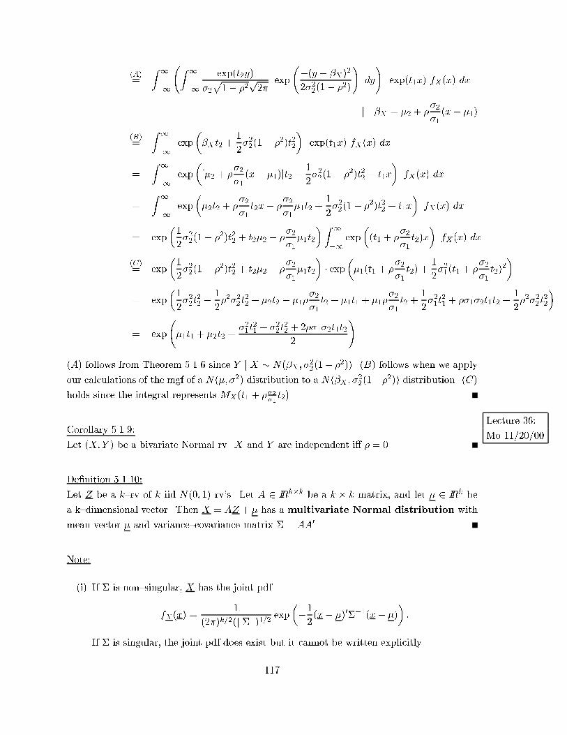
(A)=

Z 1

�1

Z 1

�1

exp(t2y)

�2

p1� �2

p2�

exp

�(y � �X)

2

2�22(1� �2)

!dy

!exp(t1x) fX(x) dx

j �X = �2 + ��2

�1(x� �1)

(B)=

Z 1

�1exp

��X t2 +

1

2�22(1� �

2)t22

�exp(t1x) fX(x) dx

=

Z 1

�1exp

�[�2 + �

�2

�1(x� �1)]t2 +

1

2�22(1� �

2)t22 + t1x

�fX(x) dx

=

Z 1

�1exp

��2t2 + �

�2

�1t2x� �

�2

�1�1t2 +

1

2�22(1� �

2)t22 + t1x

�fX(x) dx

= exp

�1

2�22(1� �

2)t22 + t2�2 � ��2

�1�1t2

�Z 1

�1exp

�(t1 + �

�2

�1t2)x

�fX(x) dx

(C)= exp

�1

2�22(1� �

2)t22 + t2�2 � ��2

�1�1t2

�� exp

��1(t1 + �

�2

�1t2) +

1

2�21(t1 + �

�2

�1t2)

2

�

= exp

�1

2�22t22 �

1

2�2�22t22 + �2t2 � �1�

�2

�1t2 + �1t1 + �1�

�2

�1t2 +

1

2�21t21 + ��1�2t1t2 +

1

2�2�22t22

�

= exp

�1t1 + �2t2 +

�21t21 + �

22t22 + 2��1�2t1t2

2

!

(A) follows from Theorem 5.1.6 since Y j X � N(�X ; �22(1� �

2)). (B) follows when we apply

our calculations of the mgf of a N(�; �2) distribution to a N(�X ; �22(1��

2)) distribution. (C)

holds since the integral represents MX(t1 + ��2�1t2).

Lecture 36:

Mo 11/20/00Corollary 5.1.9:

Let (X;Y ) be a bivariate Normal rv. X and Y are independent i� � = 0.

De�nition 5.1.10:

Let Z be a k{rv of k iid N(0; 1) rv's. Let A 2 IRk�k be a k � k matrix, and let � 2 IR

k be

a k{dimensional vector. Then X = AZ + � has a multivariate Normal distribution with

mean vector � and variance{covariance matrix � = AA0.

Note:

(i) If � is non{singular, X has the joint pdf

fX(x) =1

(2�)k=2(j � j)1=2exp

��1

2(x� �)0��1(x� �)

�:

If � is singular, the joint pdf does exist but it cannot be written explicitly.

117

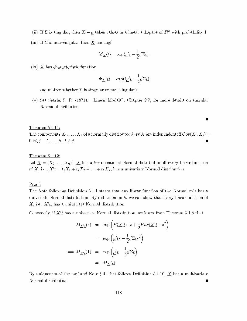
(ii) If � is singular, then X � � takes values in a linear subspace of IRk with probability 1.

(iii) If � is non{singular, then X has mgf

MX(t) = exp(�0t+1

2t0�t):

(iv) X has characteristic function

�X(t) = exp(i�0t� 1

2t0�t)

(no matter whether � is singular or non{singular).

(v) See Searle, S. R. (1971): \Linear Models", Chapter 2.7, for more details on singular

Normal distributions.

Theorem 5.1.11:

The componentsX1; : : : ;Xk of a normally distributed k{rvX are independent i�Cov(Xi;Xj) =

0 8i; j = 1; : : : ; k; i 6= j.

Theorem 5.1.12:

Let X = (X1; : : : ;Xk)0. X has a k{dimensional Normal distribution i� every linear function

of X, i.e., X 0t = t1X1 + t2X2 + : : : + tkXk, has a univariate Normal distribution.

Proof:

The Note following De�nition 5.1.1 states that any linear function of two Normal rv's has a

univariate Normal distribution. By induction on k, we can show that every linear function of

X, i.e., X 0t, has a univariate Normal distribution.

Conversely, if X 0t has a univariate Normal distribution, we know from Theorem 5.1.8 that

MX0t(s) = exp

�E(X 0

t) � s+ 1

2V ar(X 0

t) � s2�

= exp

��0ts+

1

2t0�ts2

�

=)MX0t(1) = exp

��0t+

1

2t0�t�

= MX(t)

By uniqueness of the mgf and Note (iii) that follows De�nition 5.1.10, X has a multivariate

Normal distribution.

118

5.2 Exponential Family of Distributions

De�nition 5.2.1:

Let # be an interval on the real line. Let ff(�; �) : � 2 #g be a family of pdf's (or pmf's). We

assume that the set fx : f(x; �) > 0g is independent of �, where x = (x1; : : : ; xn).

We say that the family ff(�; �) : � 2 #g is a one{parameter exponential family if there

exist real{valued functions Q(�) and D(�) on # and Borel{measurable functions T (X) and

S(X) on IRn such that

f(x; �) = exp(Q(�)T (x) +D(�) + S(x)):

Note:

We can also write f(x; �) as

f(x; �) = h(x)c(�) exp(�T (x))

where h(x) = exp(S(x)), � = Q(�), and c(�) = exp(D(Q�1(�))), and call this the exponen-

tial family in canonical form for a natural parameter �.

De�nition 5.2.2:

Let # � IRk be a k{dimensional interval. Let ff(�; �) : � 2 #g be a family of pdf's (or pmf's).

We assume that the set fx : f(x; �) > 0g is independent of �, where x = (x1; : : : ; xn).

We say that the family ff(�; �) : � 2 #g is a k{parameter exponential family if there

exist real{valued functions Q1(�); : : : Qk(�) and D(�) on # and Borel{measurable functions

T1(X); : : : ; Tk(X) and S(X) on IRn such that

f(x; �) = exp

kXi=1

Qi(�)Ti(x) +D(�) + S(x)

!:

Note:

Similar to the Note following De�nition 5.2.1, we can express the k{parameter exponential

family in canonical form for a natural k � 1 parameter vector � = (�1; : : : ; �k)0.

119

Example 5.2.3:

Let X � N(�; �2) with both parameters � and �2 unknown. We have:

f(x; �) =1p2��2

exp

�� 1

2�2(x� �)2

�= exp

� 1

2�2x2 +

�

�2x� �

2

2�2� 1

2ln(2��2)

!

� = (�; �2)

# = f(�; �2) : � 2 IR; �2> 0g

Therefore,

Q1(�) = � 1

2�2

T1(x) = x2

Q2(�) =�

�2

T2(x) = x

D(�) = � �2

2�2� 1

2ln(2��2)

S(x) = 0

Thus, this is a 2{parameter exponential family.

120

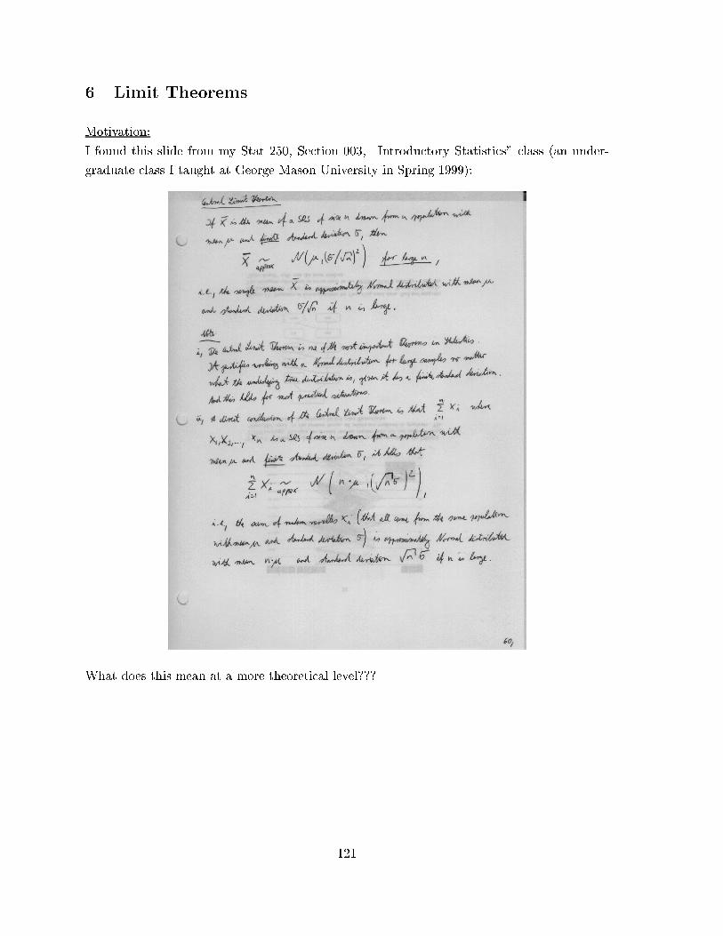
6 Limit Theorems

Motivation:

I found this slide from my Stat 250, Section 003, \Introductory Statistics" class (an under-

graduate class I taught at George Mason University in Spring 1999):

What does this mean at a more theoretical level???

121

Lecture 37:

Mo 11/27/006.1 Modes of Convergence

De�nition 6.1.1:

Let X1; : : : ;Xn be iid rv's with common cdf FX(x). Let T = T (X) be any statistic, i.e., a

Borel{measurable function of X that does not involve the population parameter(s) #, de�ned

on the support X of X . The induced probability distribution of T (X) is called the sampling

distribution of T (X).

Note:

(i) Commonly used statistics are:

Sample Mean: Xn =1n

nXi=1

Xi

Sample Variance: S2n =1

n�1

nXi=1

(Xi �Xn)2

Sample Median, Order Statistics, Min, Max, etc.

(ii) Recall that if X1; : : : ; Xn are iid and if E(X) and V ar(X) exist, then E(Xn) = � =

E(X), E(S2n) = �2 = V ar(X), and V ar(Xn) =

�2

n.

(iii) Recall that ifX1; : : : ;Xn are iid and ifX has mgfMX(t) or characteristic function �X(t)

then MXn(t) = (MX(

tn))

n or �Xn(t) = (�X(

tn))

n.

Note: Let fXng1n=1 be a sequence of rv's on some probability space (; L; P ). Is there any

meaning behind the expression limn!1Xn = X? Not immediately under the usual de�nitions

of limits. We �rst need to de�ne modes of convergence for rv's and probabilities.

De�nition 6.1.2:

Let fXng1n=1 be a sequence of rv's with cdf's fFng1n=1 and let X be a rv with cdf F . If

Fn(x) ! F (x) at all continuity points of F , we say that Xn converges in distribution to

X (Xnd�! X) or Xn converges in law to X (Xn

L�! X), or Fn converges weakly to F

(Fnw�! F ).

Example 6.1.3:

Let Xn � N(0; 1n). Then

Fn(x) =

Z x

�1

exp��1

2nt2�

q2�n

dt

122

=

Z pnx

�1

exp(�12s

2)p2�

ds

= �(pnx)

=) Fn(x) !

8>><>>:

�(1) = 1; if x > 0

�(0) = 12 ; if x = 0

�(�1) = 0; if x < 0

If FX(x) =

(1; x � 0

0; x < 0the only point of discontinuity is at x = 0. Everywhere else,

�(pnx) = Fn(x)! FX(x).

So, Xnd�! X, where P (X = 0) = 1, or Xn

d�! 0 since the limiting rv here is degenerate,

i.e., it has a Dirac(0) distribution.

Example 6.1.4:

In this example, the sequence fFng1n=1 converges pointwise to something that is not a cdf:

Let Xn � Dirac(n), i.e., P (Xn = n) = 1. Then,

Fn(x) =

(0; x < n

1; x � n

It is Fn(x)! 0 8x which is not a cdf. Thus, there is no rv X such that Xnd�! X.

Example 6.1.5:

Let fXng1n=1 be a sequence of rv's such that P (Xn = 0) = 1� 1nand P (Xn = n) = 1

nand let

X � Dirac(0), i.e., P (X = 0) = 1.

It is

Fn(x) =

8>><>>:

0; x < 0

1� 1n; 0 � x < n

1; x � n

FX(x) =

(0; x < 0

1; x � 0

It holds that Fnw�! FX but

E(Xkn) = n

k�1 6! E(Xk) = 0:

Thus, convergence in distribution does not imply convergence of moments/means.

123

Note:

Convergence in distribution does not say that the Xi's are close to each other or to X. It only

means that their cdf's are (eventually) close to some cdf F . The Xi's do not even have to be

de�ned on the same probability space.

Example 6.1.6:

Let X and fXng1n=1 be iid N(0; 1). Obviously, Xnd�! X but lim

n!1Xn 6= X.

Theorem 6.1.7:

Let X and fXng1n=1 be discrete rv's with support X and fXng1n=1, respectively. De�ne

the countable set A = X [1[n=1

Xn = fak : k = 1; 2; 3; : : :g. Let pk = P (X = ak) and

pnk = P (Xn = ak). Then it holds that pnk ! pk 8k i� Xnd�! X.

Theorem 6.1.8:

LetX and fXng1n=1 be continuous rv's with pdf's f and ffng1n=1, respectively. If fn(x)! f(x)

for almost all x as n!1 then Xnd�! X.

Theorem 6.1.9:

Let X and fXng1n=1 be rv's such that Xnd�! X. Let c 2 IR be a constant. Then it holds:

(i) Xn + cd�! X + c.

(ii) cXnd�! cX.

(iii) If an ! a and bn ! b, then anXn + bnd�! aX + b.

Proof:

Part (iii):

Suppose that a > 0; an > 0. (If a < 0; an < 0, the result follows via (ii) and c = �1.)Let Yn = anXn + bn and Y = aX + b. It is

FY (y) = P (Y < y) = P (aX + b < y) = P (X <y � b

a) = FX(

y � b

a):

Likewise,

FYn(y) = FXn(y � bn

an):

If y is a continuity point of FY ,y�ba

is a continuity point of FX . Since an ! a; bn ! b and

FXn(x) ! FX(x), it follows that FYn(y) ! FY (y) for every continuity point y of FY . Thus,

anXn + bnd�! aX + b.

124

Lecture 38:

We 11/29/00De�nition 6.1.10:

Let fXng1n=1 be a sequence of rv's de�ned on a probability space (; L; P ). We say that Xn

converges in probability to a rv X (Xnp�! X, P- lim

n!1Xn = X) if

limn!1P (j Xn �X j> �) = 0 8� > 0:

Note:

The following are equivalent:

limn!1P (j Xn �X j> �) = 0

() limn!1P (j Xn �X j� �) = 1

() limn!1P (f! : j Xn(!)�X(!) j> �)) = 0

If X is degenerate, i.e., P (X = c) = 1, we say that Xn is consistent for c. For example, let

Xn such that P (Xn = 0) = 1� 1n and P (Xn = 1) = 1

n . Then

P (j Xn j> �) =

(1n ; 0 < � < 1

0; � � 1

Therefore, limn!1P (j Xn j> �) = 0 8� > 0. So Xn

p�! 0, i.e., Xn is consistent for 0.

Theorem 6.1.11:

(i) Xnp�! X () Xn �X

p�! 0.

(ii) Xnp�! X;Xn

p�! Y =) P (X = Y ) = 1.

(iii) Xnp�! X;Xm

p�! X =) Xn �Xmp�! 0 as n;m!1.

(iv) Xnp�! X;Yn

p�! Y =) Xn � Ynp�! X � Y .

(v) Xnp�! X; k 2 IR a constant =) kXn

p�! kX.

(vi) Xnp�! k; k 2 IR a constant =) X

rn

p�! kr 8r 2 IN .

(vii) Xnp�! a; Yn

p�! b; a; b 2 IR =) XnYnp�! ab.

(viii) Xnp�! 1 =) X

�1n

p�! 1.

(ix) Xnp�! a; Yn

p�! b; a 2 IR; b 2 IR� f0g =) Xn

Yn

p�! ab .

125

(x) Xnp�! X;Y an arbitrary rv =) XnY

p�! XY .

(xi) Xnp�! X;Yn

p�! Y =) XnYnp�! XY .

Proof:

See Rohatgi, page 244{245 for partial proofs.

Theorem 6.1.12:

Let Xnp�! X and let g be a continuous function on IR. Then g(Xn)

p�! g(X).

Proof:

Preconditions:

1.) X rv =) 8� > 0 9k = k(�) : P (jXj > k) < �2

2.) g is continuous on IR

=) g is also uniformly continuous on [�k; k] (see De�nition of uniformly continuousin Theorem 3.3.3 (iii))

=) 9� = �(�; k) : jXj � k; jXn �Xj < � ) jg(Xn)� g(X)j < �

Let

A = fjXj � kg = f! : jX(!)j � kg

B = fjXn �Xj < �g = f! : jXn(!)�X(!)j < �g

C = fjg(Xn)� g(X)j < �g = f! : jg(Xn(!))� g(X(!))j < �g

If ! 2 A \B2:)=) ! 2 C

=) A \B � C

=) CC � (A \B)C = A

C [BC

=) P (CC) � P (AC [BC) � P (AC) + P (BC)

Now:

P (jg(Xn)� g(X)j � �) � P (jXj > k)| {z }� �2by 1.)

+ P (jXn �Xj � �)| {z }� �2for n�n0(�;�;k) since Xn

p�!X

� � for n � n0(�; �; k)

Corollary 6.1.13:

Let Xnp�! c; c 2 IR and let g be a continuous function on IR. Then g(Xn)

p�! g(c).

126

Theorem 6.1.14:

Xnp�! X =) Xn

d�! X.

Proof:

Xnp�! X , P (jXn �Xj > �)! 0 as n!1 8� > 0

It holds:

P (X � x� �) = P (X � x� �; jXn �Xj � �) + P (X � x� �; jXn �Xj > �)

(A)

� P (Xn � x) + P (jXn �Xj > �)

(A) holds since X � x� � and Xn within � of X, thus Xn � x.

Similarly, it holds:

P (Xn � x) = P (Xn � x; j Xn �X j� �) + P (Xn � x; j Xn �X j> �)

� P (X � x+ �) + P (jXn �Xj > �)

Combining the 2 inequalities from above gives:

P (X � x� �)� P (jXn �Xj > �)| {z }!0 as n!1

� P (Xn � x)| {z }=Fn(x)

� P (X � x+ �) + P (jXn �Xj > �)| {z }!0 as n!1

Therefore,

P (X � x� �) � Fn(x) � P (X � x+ �) as n!1:

Since the cdf's Fn(�) are not necessarily left continuous, we get the following result for � # 0:

P (X < x) � Fn(x) � P (X � x) = FX(x)

Let x be a continuity point of F . Then it holds:

F (x) = P (X < x) � Fn(x) � F (x)

=) Fn(x)! F (x)

=) Xnd�! X

Theorem 6.1.15:

Let c 2 IR be a constant. Then it holds:

Xnd�! c() Xn

p�! c:

127

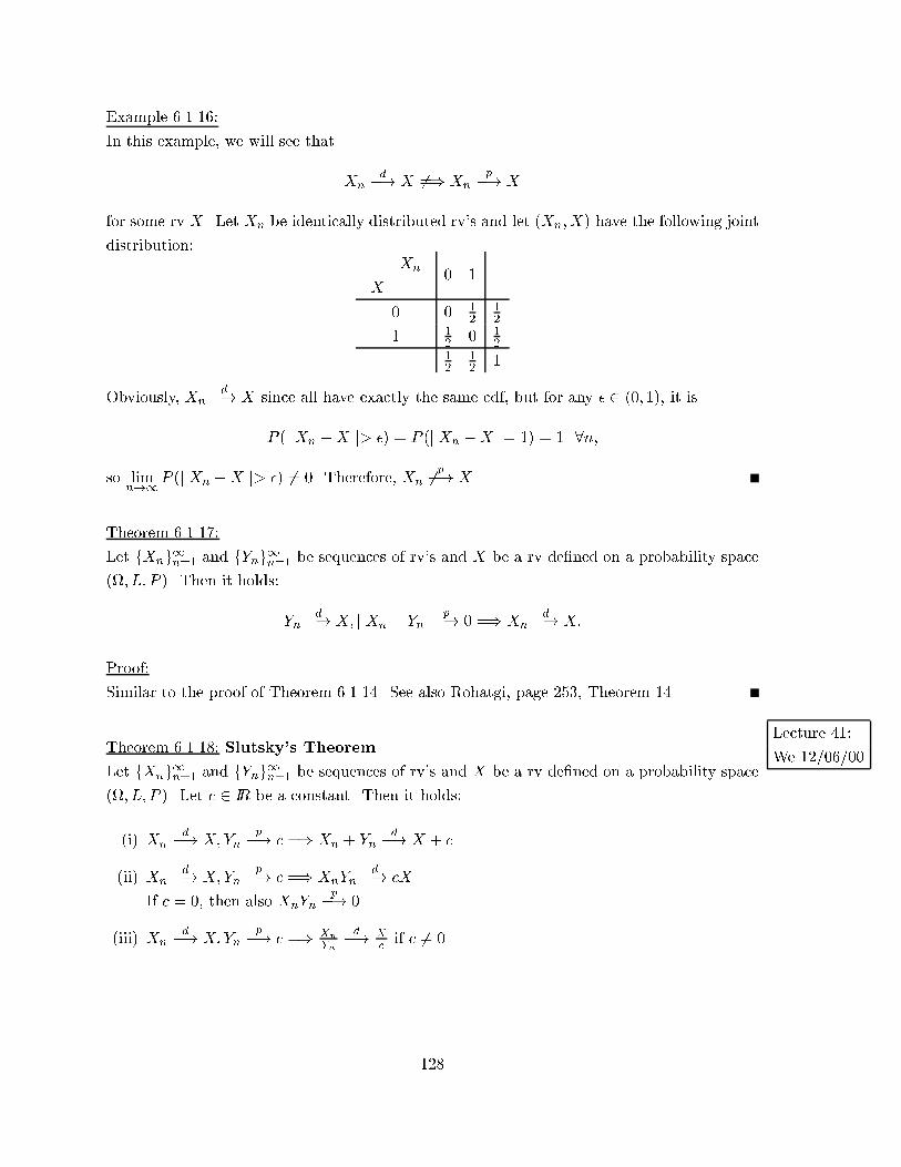
Example 6.1.16:

In this example, we will see that

Xnd�! X 6=) Xn

p�! X

for some rv X. Let Xn be identically distributed rv's and let (Xn;X) have the following joint

distribution:Xn

X0 1

0 0 12

12

1 12 0 1

212

12 1

Obviously, Xnd�! X since all have exactly the same cdf, but for any � 2 (0; 1), it is

P (j Xn �X j> �) = P (j Xn �X j= 1) = 1 8n;

so limn!1P (j Xn �X j> �) 6= 0. Therefore, Xn 6

p�! X.

Theorem 6.1.17:

Let fXng1n=1 and fYng1n=1 be sequences of rv's and X be a rv de�ned on a probability space

(; L; P ). Then it holds:

Ynd�! X; j Xn � Yn j

p�! 0 =) Xnd�! X:

Proof:

Similar to the proof of Theorem 6.1.14. See also Rohatgi, page 253, Theorem 14.

Lecture 41:

We 12/06/00Theorem 6.1.18: Slutsky's Theorem

Let fXng1n=1 and fYng1n=1 be sequences of rv's and X be a rv de�ned on a probability space

(; L; P ). Let c 2 IR be a constant. Then it holds:

(i) Xnd�! X;Yn

p�! c =) Xn + Ynd�! X + c.

(ii) Xnd�! X;Yn

p�! c =) XnYnd�! cX.

If c = 0, then also XnYnp�! 0.

(iii) Xnd�! X;Yn

p�! c =) Xn

Yn

d�! Xc if c 6= 0.

128

Proof:

(i) Ynp�! c

Th:6:1:11(i)() Yn � cp�! 0

=) Yn � c = Yn + (Xn �Xn)� c = (Xn + Yn)� (Xn + c)p�! 0 (A)

Xnd�! X

Th:6:1:9(i)=) Xn + c

d�! X + c (B)

Combining (A) and (B), it follows from Theorem 6.1.17:

Xn + Ynd�! X + c

(ii) Case c = 0:

8� > 0 8k > 0, it is

P (j XnYn j> �) = P (j XnYn j> �; Yn ��

k) + P (j XnYn j> �; Yn >

�

k)

� P (j Xn�

kj> �) + P (Yn >

�

k)

� P (j Xn j> k) + P (j Yn j>�

k)

Since Xnd�! X and Yn

p�! 0, it follows

limn!1P (j XnYn j> �) � P (j Xn j> k)! 0 as k !1:

Therefore, XnYnp�! 0.

Case c 6= 0:

Since Xnd�! X and Yn

p�! c, it follows from (ii), case c = 0, that XnYn � cXn =

Xn(Yn � c)p�! 0.

=) XnYnp�! cXn

Th:6:1:14=) XnYn

d�! cXn

Since cXnd�! cX by Theorem 6.1.9 (ii), it follows from Theorem 6.1.17:

XnYnd�! cX

(iii) Let Znp�! 1 and let Yn = cZn.

c6=0=) 1

Yn= 1

Zn� 1c

Th:6:1:11(v;viii)=) 1

Yn

p�! 1c

With part (ii) above, it follows:

Xnd�! X and 1

Yn

p�! 1c

=) Xn

Yn

d�! Xc

129

De�nition 6.1.19:

Let fXng1n=1 be a sequence of rv's such that E(j Xn jr) <1 for some r > 0. We say that Xn

converges in the rth mean to a rv X (Xn

r�! X) if E(j X jr) <1 and

limn!1E(j Xn �X jr) = 0:

Example 6.1.20:

Let fXng1n=1 be a sequence of rv's de�ned by P (Xn = 0) = 1� 1nand P (Xn = 1) = 1

n.

It is E(j Xn jr) = 1n8r > 0. Therefore, Xn

r�! 0 8r > 0.

Note:

The special cases r = 1 and r = 2 are called convergence in absolute mean for r = 1

(Xn1�! X) and convergence in mean square for r = 2 (Xn

ms�! X or Xn2�! X).

Theorem 6.1.21:

Assume that Xnr�! X for some r > 0. Then Xn

p�! X.

Proof:

Using Markov's Inequality (Corollary 3.5.2), it holds for any � > 0:

E(j Xn �X jr)�r

� P (j Xn �X j� �)

Xnr�! X =) lim

n!1E(j Xn �X jr) = 0

=) limn!1P (j Xn �X j� �) � lim

n!1E(j Xn �X jr)

�r= 0

=) Xnp�! X

Example 6.1.22:

Let fXng1n=1 be a sequence of rv's de�ned by P (Xn = 0) = 1 � 1nr and P (Xn = n) = 1

nr for

some r > 0.

For any � > 0, P (j Xn j> �)! 0 as n!1; so Xnp�! 0.

For 0 < s < r, E(j Xn js) = 1nr�s

! 0 as n ! 1; so Xns�! 0. But E(j Xn jr) = 1 6! 0 as

n!1; so Xn 6r�! 0.

130

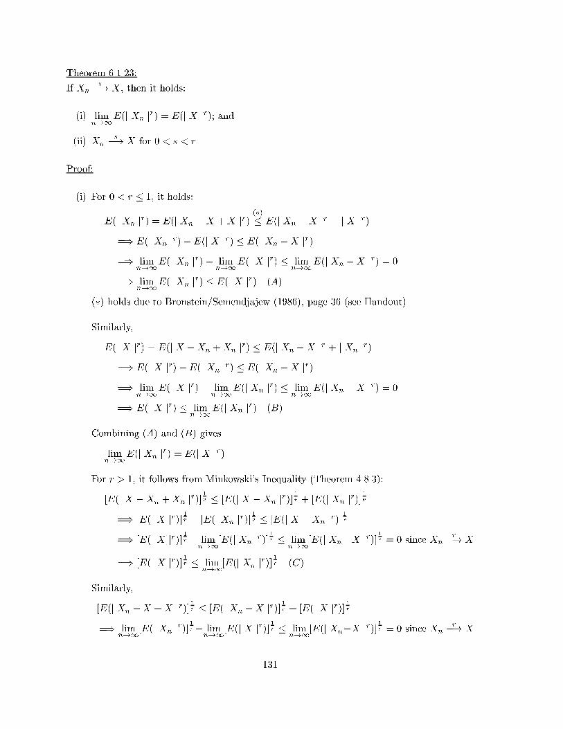
Theorem 6.1.23:

If Xnr�! X, then it holds:

(i) limn!1E(j Xn jr) = E(j X jr); and

(ii) Xns�! X for 0 < s < r.

Proof:

(i) For 0 < r � 1, it holds:

E(j Xn jr) = E(j Xn �X +X jr)(�)� E(j Xn �X jr + j X jr)

=) E(j Xn jr)�E(j X jr) � E(j Xn �X jr)

=) limn!1E(j Xn jr)� lim

n!1E(j X jr) � limn!1E(j Xn �X jr) = 0

=) limn!1E(j Xn jr) � E(j X jr) (A)

(�) holds due to Bronstein/Semendjajew (1986), page 36 (see Handout)

Similarly,

E(j X jr) = E(j X �Xn +Xn jr) � E(j Xn �X jr + j Xn jr)

=) E(j X jr)�E(j Xn jr) � E(j Xn �X jr)

=) limn!1E(j X jr)� lim

n!1E(j Xn jr) � limn!1E(j Xn �X jr) = 0

=) E(j X jr) � limn!1E(j Xn jr) (B)

Combining (A) and (B) gives

limn!1E(j Xn jr) = E(j X jr)

For r > 1, it follows from Minkowski's Inequality (Theorem 4.8.3):

[E(j X �Xn +Xn jr)]1r � [E(j X �Xn jr)]

1r + [E(j Xn jr)]

1r

=) [E(j X jr)] 1r � [E(j Xn jr)]1r � [E(j X �Xn jr)]

1r

=) [E(j X jr)] 1r � limn!1[E(j Xn jr)]

1r � lim

n!1[E(j Xn�X jr)]1r = 0 since Xn

r�! X

=) [E(j X jr)] 1r � limn!1[E(j Xn jr)]

1r (C)

Similarly,

[E(j Xn �X +X jr)] 1r � [E(j Xn �X jr)] 1r + [E(j X jr)] 1r

=) limn!1[E(j Xn jr)]

1r� lim

n!1[E(j X jr)]1r � lim

n!1[E(j Xn�X jr)]1r = 0 since Xn

r�! X

131

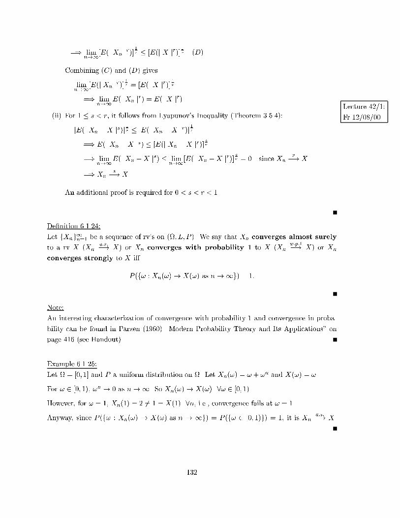
=) limn!1[E(j Xn jr)]

1r � [E(j X jr)]

1r (D)

Combining (C) and (D) gives

limn!1[E(j Xn jr)]

1r = [E(j X jr)]

1r

=) limn!1E(j Xn jr) = E(j X jr)

Lecture 42/1:

Fr 12/08/00(ii) For 1 � s < r, it follows from Lyapunov's Inequality (Theorem 3.5.4):

[E(j Xn �X js)] 1s � [E(j Xn �X jr)] 1r

=) E(j Xn �X js) � [E(j Xn �X jr)] sr

=) limn!1E(j Xn �X js) � lim

n!1[E(j Xn �X jr)]sr = 0 since Xn

r�! X

=) Xns�! X

An additional proof is required for 0 < s < r < 1.

De�nition 6.1.24:

Let fXng1n=1 be a sequence of rv's on (; L; P ). We say that Xn converges almost surely

to a rv X (Xna:s:�! X) or Xn converges with probability 1 to X (Xn

w:p:1�! X) or Xn

converges strongly to X i�

P (f! : Xn(!)! X(!) as n!1g) = 1:

Note:

An interesting characterization of convergence with probability 1 and convergence in proba-

bility can be found in Parzen (1960) \Modern Probability Theory and Its Applications" on

page 416 (see Handout).

Example 6.1.25:

Let = [0; 1] and P a uniform distribution on . Let Xn(!) = ! + !n and X(!) = !.

For ! 2 [0; 1), !n ! 0 as n!1. So Xn(!)! X(!) 8! 2 [0; 1).

However, for ! = 1, Xn(1) = 2 6= 1 = X(1) 8n, i.e., convergence fails at ! = 1.

Anyway, since P (f! : Xn(!) ! X(!) as n ! 1g) = P (f! 2 [0; 1)g) = 1, it is Xna:s:�! X.

132

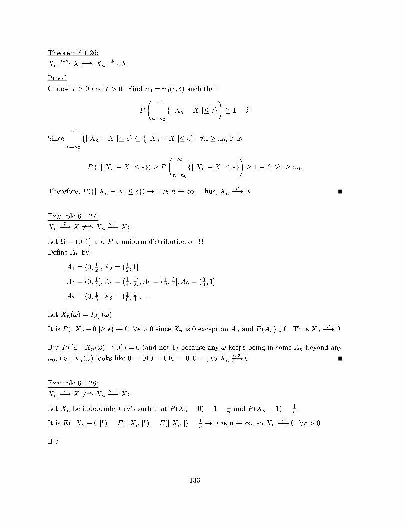
Theorem 6.1.26:

Xna:s:�! X =) Xn

p�! X.

Proof:

Choose � > 0 and � > 0. Find n0 = n0(�; �) such that

P

1\n=n0

fj Xn �X j� �g!� 1� �:

Since1\

n=n0

fj Xn �X j� �g � fj Xn �X j� �g 8n � n0, it is

P (fj Xn �X j� �g) � P

1\n=n0

fj Xn �X j� �g!� 1� � 8n � n0:

Therefore, P (fj Xn �X j� �g)! 1 as n!1. Thus, Xnp�! X.

Example 6.1.27:

Xnp�! X 6=) Xn

a:s:�! X:

Let = (0; 1] and P a uniform distribution on .

De�ne An by

A1 = (0; 12 ]; A2 = (12 ; 1]

A3 = (0; 14 ]; A4 = (14 ;12 ]; A5 = (12 ;

34 ]; A6 = (34 ; 1]

A7 = (0; 18 ]; A8 = (18 ;14 ]; : : :

Let Xn(!) = IAn(!).

It is P (j Xn� 0 j� �)! 0 8� > 0 since Xn is 0 except on An and P (An) # 0. Thus Xnp�! 0.

But P (f! : Xn(!)! 0g) = 0 (and not 1) because any ! keeps being in some An beyond any

n0, i.e., Xn(!) looks like 0 : : : 010 : : : 010 : : : 010 : : :, so Xn 6a:s:�! 0.

Example 6.1.28:

Xnr�! X 6=) Xn

a:s:�! X:

Let Xn be independent rv's such that P (Xn = 0) = 1� 1n and P (Xn = 1) = 1

n .

It is E(j Xn � 0 jr) = E(j Xn jr) = E(j Xn j) = 1n! 0 as n!1, so Xn

r�! 0 8r > 0.

But

133

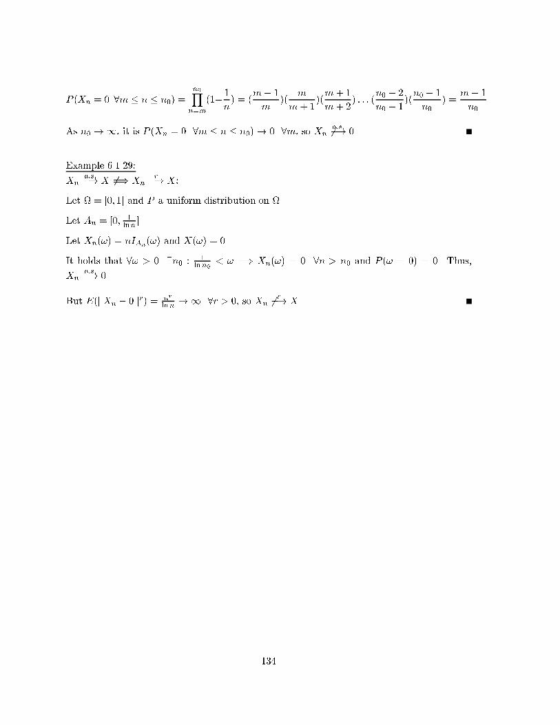
P (Xn = 0 8m � n � n0) =

n0Yn=m

(1� 1

n) = (

m� 1

m)(

m

m+ 1)(m+ 1

m+ 2) : : : (

n0 � 2

n0 � 1)(n0 � 1

n0) =

m� 1

n0

As n0 !1, it is P (Xn = 0 8m � n � n0)! 0 8m, so Xn 6a:s:�! 0.

Example 6.1.29:

Xna:s:�! X 6=) Xn

r�! X:

Let = [0; 1] and P a uniform distribution on .

Let An = [0; 1lnn ].

Let Xn(!) = nIAn(!) and X(!) = 0.

It holds that 8! > 0 9n0 : 1lnn0

< ! =) Xn(!) = 0 8n > n0 and P (! = 0) = 0. Thus,

Xna:s:�! 0.

But E(j Xn � 0 jr) = nr

lnn !1 8r > 0, so Xn 6r�! X.

134

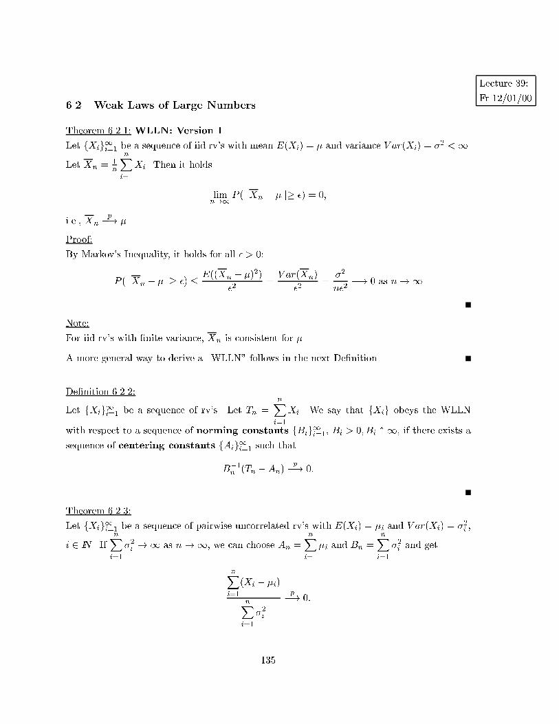
Lecture 39:

Fr 12/01/006.2 Weak Laws of Large Numbers

Theorem 6.2.1: WLLN: Version I

Let fXig1i=1 be a sequence of iid rv's with mean E(Xi) = � and variance V ar(Xi) = �2<1.

Let Xn =1n

nXi=1

Xi. Then it holds

limn!1P (j Xn � � j� �) = 0;

i.e., Xnp�! �.

Proof:

By Markov's Inequality, it holds for all � > 0:

P (j Xn � � j� �) � E((Xn � �)2)

�2=

V ar(Xn)

�2=

�2

n�2�! 0 as n!1

Note:

For iid rv's with �nite variance, Xn is consistent for �.

A more general way to derive a \WLLN" follows in the next De�nition.

De�nition 6.2.2:

Let fXig1i=1 be a sequence of rv's. Let Tn =nXi=1

Xi. We say that fXig obeys the WLLN

with respect to a sequence of norming constants fBig1i=1, Bi > 0; Bi " 1, if there exists a

sequence of centering constants fAig1i=1 such that

B�1n (Tn �An)

p�! 0:

Theorem 6.2.3:

Let fXig1i=1 be a sequence of pairwise uncorrelated rv's with E(Xi) = �i and V ar(Xi) = �2i ,

i 2 IN . IfnXi=1

�2i !1 as n!1, we can choose An =

nXi=1

�i and Bn =nXi=1

�2i and get

nXi=1

(Xi � �i)

nXi=1

�2i

p�! 0:

135

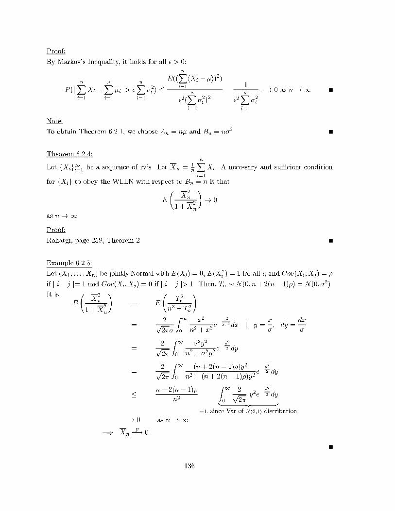
Proof:

By Markov's Inequality, it holds for all � > 0:

P (jnXi=1

Xi �nXi=1

�i j> �

nXi=1

�2i ) �

E((nXi=1

(Xi � �))2)

�2(nXi=1

�2i )2

=1

�2nXi=1

�2i

�! 0 as n!1

Note:

To obtain Theorem 6.2.1, we choose An = n� and Bn = n�2.

Theorem 6.2.4:

Let fXig1i=1 be a sequence of rv's. Let Xn = 1n

nXi=1

Xi. A necessary and su�cient condition

for fXig to obey the WLLN with respect to Bn = n is that

E

X

2n

1 +X2n

!! 0

as n!1.

Proof:

Rohatgi, page 258, Theorem 2.

Example 6.2.5:

Let (X1; : : : ;Xn) be jointly Normal with E(Xi) = 0, E(X2i ) = 1 for all i, and Cov(Xi;Xj) = �

if j i� j j= 1 and Cov(Xi; Xj) = 0 if j i� j j> 1. Then, Tn � N(0; n+2(n� 1)�) = N(0; �2).

It is

E

X

2n

1 +X2n

!= E

T2n

n2 + T 2n

!

=2p2��

Z 1

0

x2

n2 + x2e� x2

2�2 dx j y =x

�; dy =

dx

�

=2p2�

Z 1

0

�2y2

n2 + �2y2e� y2

2 dy

=2p2�

Z 1

0

(n+ 2(n� 1)�)y2

n2 + (n+ 2(n� 1)�)y2e� y2

2 dy

� n+ 2(n� 1)�

n2

Z 1

0

2p2�

y2e� y2

2 dy| {z }=1; since Var of N(0;1) distribution

! 0 as n!1

=) Xnp�! 0

136

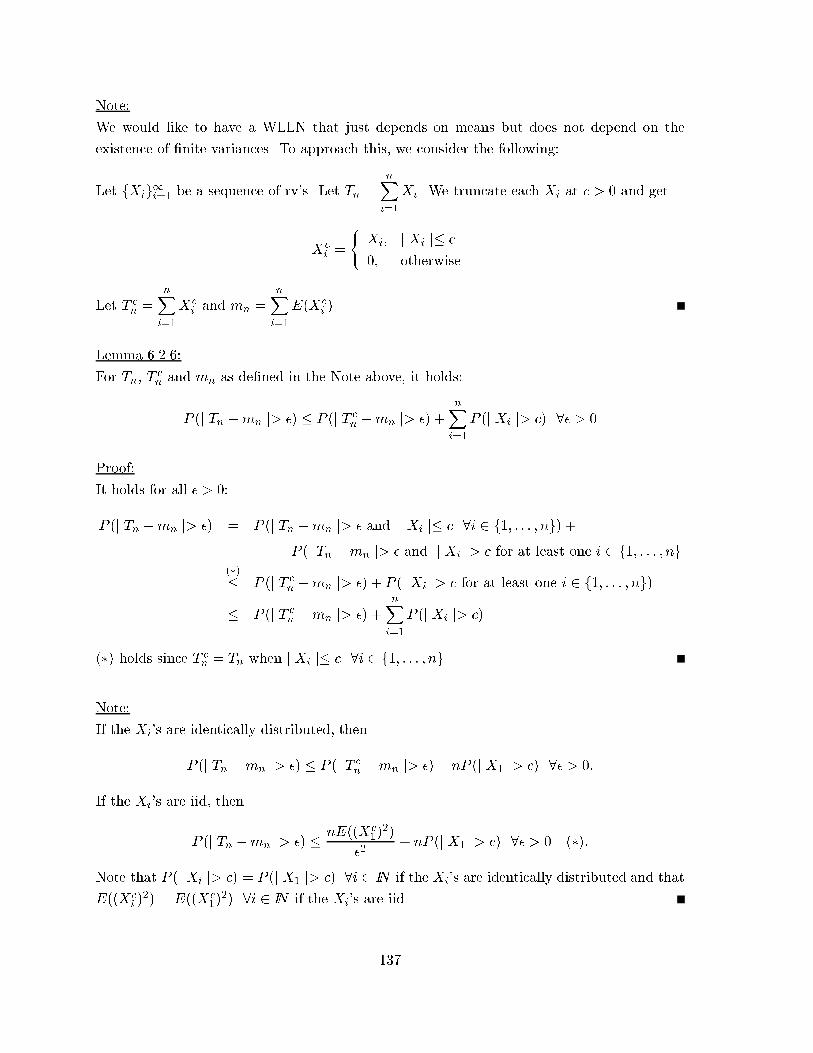
Note:

We would like to have a WLLN that just depends on means but does not depend on the

existence of �nite variances. To approach this, we consider the following:

Let fXig1i=1 be a sequence of rv's. Let Tn =nXi=1

Xi. We truncate each Xi at c > 0 and get

Xci =

(Xi; j Xi j� c

0; otherwise

Let T cn =

nXi=1

Xci and mn =

nXi=1

E(Xci ).

Lemma 6.2.6:

For Tn, Tcn and mn as de�ned in the Note above, it holds:

P (j Tn �mn j> �) � P (j T cn �mn j> �) +

nXi=1

P (j Xi j> c) 8� > 0

Proof:

It holds for all � > 0:

P (j Tn �mn j> �) = P (j Tn �mn j> � and j Xi j� c 8i 2 f1; : : : ; ng) +

P (j Tn �mn j> � and j Xi j> c for at least one i 2 f1; : : : ; ng(�)� P (j T c

n �mn j> �) + P (j Xi j> c for at least one i 2 f1; : : : ; ng)

� P (j T cn �mn j> �) +

nXi=1

P (j Xi j> c)

(�) holds since T cn = Tn when j Xi j� c 8i 2 f1; : : : ; ng.

Note:

If the Xi's are identically distributed, then

P (j Tn �mn j> �) � P (j T cn �mn j> �) + nP (j X1 j> c) 8� > 0:

If the Xi's are iid, then

P (j Tn �mn j> �) � nE((Xc1)2)

�2+ nP (j X1 j> c) 8� > 0 (�):

Note that P (j Xi j> c) = P (j X1 j> c) 8i 2 IN if the Xi's are identically distributed and that

E((Xci )2) = E((Xc

1)2) 8i 2 IN if the Xi's are iid.

137

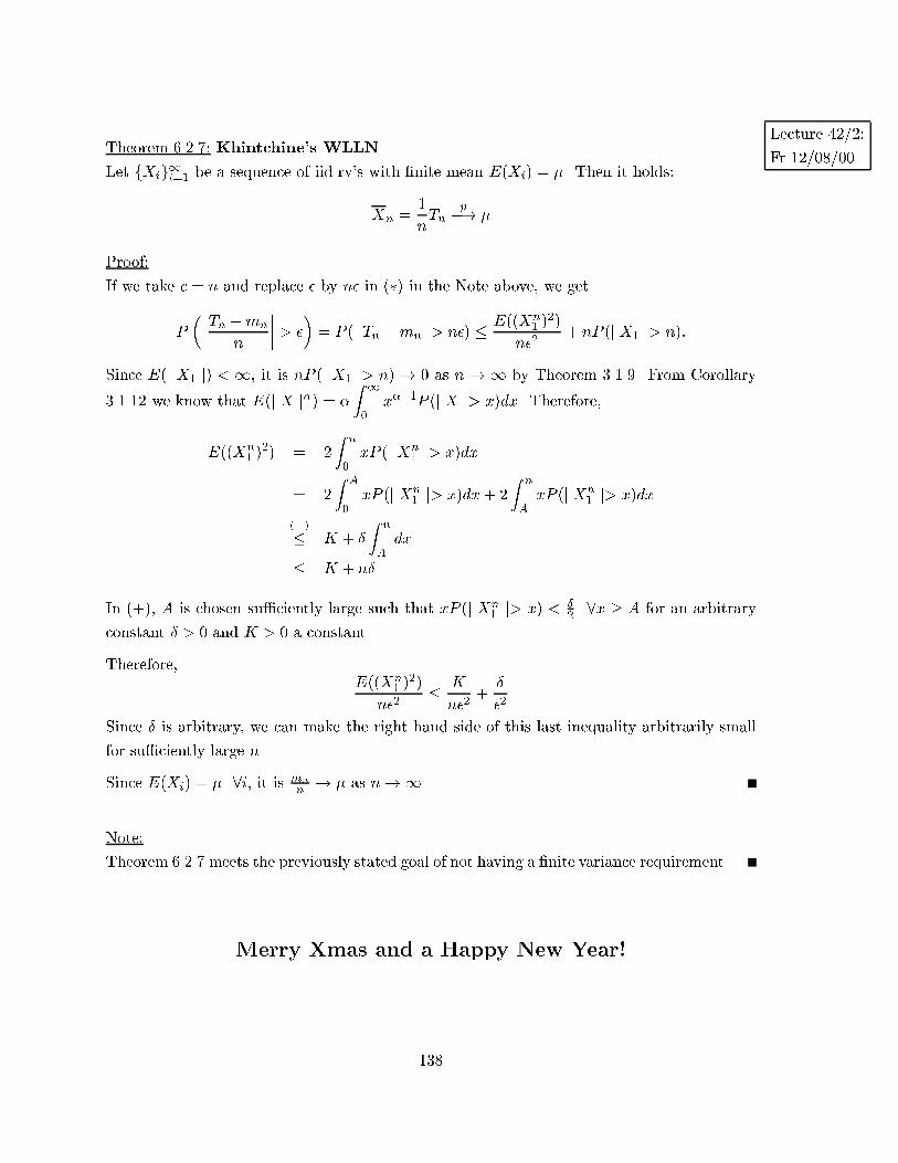
Lecture 42/2:

Fr 12/08/00Theorem 6.2.7: Khintchine's WLLN

Let fXig1i=1 be a sequence of iid rv's with �nite mean E(Xi) = �. Then it holds:

Xn =1

nTn

p�! �

Proof:

If we take c = n and replace � by n� in (�) in the Note above, we get

P

�����Tn �mn

n

���� > �

�= P (j Tn �mn j> n�) � E((Xn

1 )2)

n�2+ nP (j X1 j> n):

Since E(j X1 j) < 1, it is nP (j X1 j> n) ! 0 as n ! 1 by Theorem 3.1.9. From Corollary

3.1.12 we know that E(j X j�) = �

Z 1

0x��1

P (j X j> x)dx. Therefore,

E((Xn1 )

2) = 2

Z n

0xP (j Xn

1 j> x)dx

= 2

Z A

0xP (j Xn

1 j> x)dx+ 2

Z n

AxP (j Xn

1 j> x)dx

(+)

� K + �

Z n

Adx

� K + n�

In (+), A is chosen su�ciently large such that xP (j Xn1 j> x) < �

2 8x � A for an arbitrary

constant � > 0 and K > 0 a constant.

Therefore,E((Xn

1 )2)

n�2� K

n�2+

�

�2

Since � is arbitrary, we can make the right hand side of this last inequality arbitrarily small

for su�ciently large n.

Since E(Xi) = � 8i, it is mn

n! � as n!1.

Note:

Theorem 6.2.7 meets the previously stated goal of not having a �nite variance requirement.

Merry Xmas and a Happy New Year!

138

Index

�{Algebra, 2

�{Field, 2

�{Field, Borel, 4

�{Field, Generated, 2

k{Parameter Exponential Family, 119

kth Central Moment, 43

kth Factorial Moment, 66

kth Moment, 43

n{Dimensional Characteristic Function, 97

n{RV, 71

Absolutely Continuous, 32

Additivity, Countable, 4

Arithmetic Mean, 109

Bayes' Rule, 19

Binomial Coe�cient, 12

Binomial Theorem, 14

Bivariate Normal Distribution, 112

Bivariate RV, 72

Bochner's Theorem, 60

Bonferroni's Inequality, 7

Boole's Inequality, 9

Borel �{Field, 4

Borel Field, 2

Borel Sets, 4

Canonical Form, 119

Cauchy{Schwarz Inequality, 95

CDF, 27

CDF, Conditional, 75

CDF, Joint, 71

CDF, Marginal, 74

Centering Constants, 135

Characteristic Function, 57

Characteristic Function, n{Dimensional, 97

Chebychev's Inequality, 68

Co�nite, 2

Completely Independent, 20, 77

Complex Numbers, 56

Complex Numbers, Conjugate, 56

Complex{Valued Random Variable, 57

Concave, 108

Conditional CDF, 75

Conditional Cumulative Distribution Function, 75

Conditional Expectation, 102

Conditional PDF, 75

Conditional PMF, 74

Conditional Probability, 17

Conditional Probability Density Function, 75

Conditional Probability Mass Function, 74

Conjugate Complex Numbers, 56

Consistent, 125

Continuity of Sets, 9

Continuous, 29, 31, 32

Continuous RV, 73

Continuous, Absolutely, 32

Convergence, Almost Sure, 132

Convergence, In rth Mean, 130

Convergence, In Absolute Mean, 130

Convergence, In Distribution, 122

Convergence, In Law, 122

Convergence, In Mean Square, 130

Convergence, In Probability, 125

Convergence, Strong, 132

Convergence, Weak, 122

Convergence, With Probability 1, 132

Convex, 108

Countable Additivity, 4

Counting, Fundamental Theorem of, 11

Covariance Inequality, 111

Cumulative Distribution Function, 27

Cumulative Distribution Function, Joint, 71

Discrete, 29, 31

Discrete RV, 72

Distribution, Sampling, 122

Equally Likely, 11

Equivalence, 35

Equivalent RV, 81

Euler's Relation, 56

Event, 1

Expectation, Conditional, 102

Expectation, Multivariate, 91

Expected Value, 42

Exponential Family in Canonical Form, 119

Exponential Family, k{Parameter, 119

Exponential Family, One{Parameter, 119

Factorial, 12

Factorization Theorem, 78

Field, 1

Fundamental Theorem of Counting, 11

Geometric Mean, 109

H�older's Inequality, 106

Harmonic Mean, 109

Identically Distributed, 30

IID, 81

Implication, 35

Inclusion{Exclusion, Principle, 6

Independent, 19, 77, 78

139

Independent Identically Distributed, 81

Independent, Completely, 20, 77

Independent, Mutually, 20, 77

Independent, Pairwise, 19

Indicator Function, 34

Induced Probability, 27

Induction, 6

Induction Base, 6

Induction Step, 7

Inequality, Bonferroni's, 7

Inequality, Boole's, 9

Inequality, Cauchy{Schwarz, 95

Inequality, Chebychev's, 68

Inequality, Covariance, 111

Inequality, H�older's, 106

Inequality, Jensen's, 108

Inequality, Lyapunov's, 69

Inequality, Markov's, 68

Inequality, Minkowski's, 107

Jensen's Inequality, 108

Joint CDF, 71

Joint Cumulative Distribution Function, 71

Joint PDF, 73

Joint PMF, 72

Joint Probability Density Function, 73

Joint Probability Mass Function, 72

Jump Points, 31

Khintchine's Weak Law of Large Numbers, 138

Kolmogorov Axioms of Probability, 4

L'Hospital's Rule, 52

Law of Total Probability, 18

Lebesque's Dominated Convergence Theorem, 53

Leibnitz's Rule, 52

Levy's Theorem, 60

Logic, 35

Lyapunov's Inequality, 69

Marginal CDF, 74

Marginal Cumulative Distribution Function, 74

Marginal PDF, 73

Marginal PMF, 73

Marginal Probability Density Function, 73

Marginal Probability Mass Function, 73

Markov's Inequality, 68

MAX, 82

Mean, 42

Mean, Arithmetic, 109

Mean, Geometric, 109

Mean, Harmonic, 109

Measurable, 2, 24

Measurable L�B, 24Measurable Functions, 25

Measurable Space, 4

MGF, 50

MIN, 82

Minkowski's Inequality, 107

MMGF, 97

Moivre's Theorem, 56

Moment Generating Function, 50

Moment Generating Function, Multivariate, 97

Moment, kth, 43

Moment, kth Central, 43

Moment, kth Factorial, 66

Moment, Multi{Way, 94

Moment, Multi{Way Central, 94

Monotonic, 37

Multi{Way Central Moment, 94

Multi{Way Moment, 94

Multiplication Rule, 18

Multivariate Expectation, 91

Multivariate Moment Generating Function, 97

Multivariate Normal Distribution, 117

Multivariate RV, 72

Multivariate Transformation, 85

Mutually Independent, 20, 77

Non{Decreasing, 37

Non{Decreasing, Strictly, 37

Non{Increasing, 37

Non{Increasing, Strictly, 37

Normal Distribution, 112

Normal Distribution, Bivariate, 112

Normal Distribution, Multivariate, 117

Normal Distribution, Standard, 112

Normal Distribution, Univariate, 112

Norming Constants, 135

One{Parameter Exponential Family, 119

Order Statistic, 89

Pairwise Independent, 19

Partition, 18

PDF, 32

PDF, Conditional, 75

PDF, Joint, 73

PDF, Marginal, 73

PGF, 66

PM, 4

PMF, 31

PMF, Conditional, 74

PMF, Joint, 72

PMF, Marginal, 73

Power Set, 2

Principle of Inclusion{Exclusion, 6

Probability Density Function, 32

Probability Generating Function, 66

Probability Mass Function, 31

140

Probability Measure, 4

Probability Space, 4

Probability, Conditional, 17

Probability, Induced, 27

Probability, Total, 18

Quanti�er, 35

Random Variable, 24

Random Variable, Complex{Valued, 57

Random Vector, 24

Random Vector, n{Dimensional, 71

RV, 24

RV, Bivariate, 72

RV, Continuous, 73

RV, Discrete, 72

RV, Equivalent, 81

RV, Multivariate, 72

Sample Space, 1

Sampling Distribution, 122

Sets, Continuity of, 9

Singular, 33

Slutsky's Theorem, 128

Standard Normal Distribution, 112

Statistic, 122

Support, 37

Total Probability, 18

Transformation, 36

Transformation, Multivariate, 85

Univariate Normal Distribution, 112

Variance, 43

Variance{Covariance Matrix, 114

Weak Law Of Large Numbers, 135

Weak Law Of Large Numbers, Khintchine's, 138

141