Embed Size (px)
Citation preview

Contents
0 Introduction 5
0.1 Historical notes . . . . . . . . . . . . . . . . . . . . . . . . . . . . . . . . . . 5
0.2 On risk neutral valuation and hedging . . . . . . . . . . . . . . . . . . . . . 6
0.3 Contents . . . . . . . . . . . . . . . . . . . . . . . . . . . . . . . . . . . . . . 8
1 Single period portfolio optimization 10
1.1 Minimum variance optimization: . . . . . . . . . . . . . . . . . . . . . . . . . 12
1.2 Markowitz optimization . . . . . . . . . . . . . . . . . . . . . . . . . . . . . 15
1.3 Markowitz optimization with shortsales constraints . . . . . . . . . . . . . . 18
1.4 "Robust" optimization ** . . . . . . . . . . . . . . . . . . . . . . . . . . . . 18
1.5 Exercises . . . . . . . . . . . . . . . . . . . . . . . . . . . . . . . . . . . . . . 19
1.6 Solutions . . . . . . . . . . . . . . . . . . . . . . . . . . . . . . . . . . . . . . 20
2 Background on �nancial derivatives 21
2.1 The use of �nancial derivatives . . . . . . . . . . . . . . . . . . . . . . . . . 22
2.2 The coming of age of mathematical �nance . . . . . . . . . . . . . . . . . . . 23
2.3 The replication of derivative contracts . . . . . . . . . . . . . . . . . . . . . 24
2.4 Examples of �nancial derivatives . . . . . . . . . . . . . . . . . . . . . . . . . 27
3 Risk neutral valuation in the Cox-Ross-Rubinstein model 29
3.1 Hedging in discrete models . . . . . . . . . . . . . . . . . . . . . . . . . . . . 29
3.2 The one period binomial model . . . . . . . . . . . . . . . . . . . . . . . . . 31
3.3 Connecting the binomial and exponential Brownian motion models . . . . . 34
3.4 The multiperiod binomial model . . . . . . . . . . . . . . . . . . . . . . . . . 36
3.5 Super and sub replicating in multinomial models . . . . . . . . . . . . . . . 37
3.6 Choosing among several risk neutral measures ** . . . . . . . . . . . . . . . 39
4 Stochastic models in �nance 42
1

4.1 Levy (additive) processes . . . . . . . . . . . . . . . . . . . . . . . . . . . . . 42
4.1.1 Random walks . . . . . . . . . . . . . . . . . . . . . . . . . . . . . . 42
4.1.2 Compound Poisson processes . . . . . . . . . . . . . . . . . . . . . . 42
4.1.3 Levy processes . . . . . . . . . . . . . . . . . . . . . . . . . . . . . . 43
4.1.4 Application: Insurance premia . . . . . . . . . . . . . . . . . . . . . . 44
4.1.5 Brownian motion . . . . . . . . . . . . . . . . . . . . . . . . . . . . . 46
4.1.6 Brownian motion with drift . . . . . . . . . . . . . . . . . . . . . . . 47
4.1.7 Classi�cation of Levy processes . . . . . . . . . . . . . . . . . . . . . 49
4.2 Multiplicative (exponential) processes . . . . . . . . . . . . . . . . . . . . . . 49
4.2.1 Exponential Brownian motion . . . . . . . . . . . . . . . . . . . . . 51
4.3 Application: European �nancial derivatives . . . . . . . . . . . . . . . . . . . 54
4.3.1 Risk neutral valuation . . . . . . . . . . . . . . . . . . . . . . . . . . 55
4.3.2 Reasons for using risk neutral valuation . . . . . . . . . . . . . . . . . 57
4.3.3 A paradox concerning risk neutral valuation . . . . . . . . . . . . . . 61
4.3.4 Escher transform and valuation ** . . . . . . . . . . . . . . . . . 62
4.3.5 Path dependent derivatives: Barrier options . . . . . . . . . . . . . . 63
4.3.6 Present value when rates are stochastic: the zero coupon bond . . . 64
4.4 Conclusions . . . . . . . . . . . . . . . . . . . . . . . . . . . . . . . . . . . . 65
4.5 Exercises . . . . . . . . . . . . . . . . . . . . . . . . . . . . . . . . . . . . . . 66
4.6 Solutions . . . . . . . . . . . . . . . . . . . . . . . . . . . . . . . . . . . . . . 67
5 The method of di�erence equations for computing expectations 73
5.1 Di�erence (recurrence) equations for expectations of simple random walks . . 73
5.2 Exercises . . . . . . . . . . . . . . . . . . . . . . . . . . . . . . . . . . . . . . 77
5.3 Apendix: One dimensional linear recurrence equations with constant coeÆcients 79
5.4 Solutions . . . . . . . . . . . . . . . . . . . . . . . . . . . . . . . . . . . . . 81
6 Di�erential equations for functionals of Brownian motion 86
2

6.1 Ito's formula for Brownian motion . . . . . . . . . . . . . . . . . . . . . . . . 86
6.2 Di�erential equations used in mathematical �nance . . . . . . . . . . . . . . 91
6.2.1 Expected �nal payments . . . . . . . . . . . . . . . . . . . . . . . . . 92
6.2.2 Expected total continuous payments . . . . . . . . . . . . . . . . . . 94
6.2.3 Expected discounted �nal payments . . . . . . . . . . . . . . . . . . . 97
6.2.4 Expected present value of continuous payment ows . . . . . . . . . . 97
6.3 Summary . . . . . . . . . . . . . . . . . . . . . . . . . . . . . . . . . . . . . 97
6.4 Exercises . . . . . . . . . . . . . . . . . . . . . . . . . . . . . . . . . . . . . . 100
6.5 Solutions . . . . . . . . . . . . . . . . . . . . . . . . . . . . . . . . . . . . . . 102
7 Financial variations on Black Scholes 105
7.1 Assets on a foreign exchange . . . . . . . . . . . . . . . . . . . . . . . . . . . 105
7.2 Options on currency and on assets yielding dividends . . . . . . . . . . . . . 107
7.3 Exchange options . . . . . . . . . . . . . . . . . . . . . . . . . . . . . . . . . 108
7.4 Exercises . . . . . . . . . . . . . . . . . . . . . . . . . . . . . . . . . . . . . . 110
8 Canadian options 111
8.1 The Connection with Laplace transforms . . . . . . . . . . . . . . . . . . . . 112
8.2 American options ** . . . . . . . . . . . . . . . . . . . . . . . . . . . . . . . 116
8.3 Exercises . . . . . . . . . . . . . . . . . . . . . . . . . . . . . . . . . . . . . . 118
8.4 Solutions . . . . . . . . . . . . . . . . . . . . . . . . . . . . . . . . . . . . . . 119
1 Martingales 121
1.1 Martingales in gambling . . . . . . . . . . . . . . . . . . . . . . . . . . . . . 123
1.2 The optional stopping theorem . . . . . . . . . . . . . . . . . . . . . . . . . 123
1.3 Wald's martingale ** . . . . . . . . . . . . . . . . . . . . . . . . . . . . . . . 126
1.4 Exercises . . . . . . . . . . . . . . . . . . . . . . . . . . . . . . . . . . . . . . 128
1.5 Solutions . . . . . . . . . . . . . . . . . . . . . . . . . . . . . . . . . . . . . . 130
2 Ito's formula and Stochastic Di�erential equations 133
3

2.1 The unusual magnitude of Brownian increments . . . . . . . . . . . . . . . . 133
2.2 Di�usions . . . . . . . . . . . . . . . . . . . . . . . . . . . . . . . . . . . . . 134
2.3 The Di�erential of a Product of di�usions . . . . . . . . . . . . . . . . . . . 136
2.4 Ito's formula for general di�usions . . . . . . . . . . . . . . . . . . . . . . . . 137
2.5 Exercises . . . . . . . . . . . . . . . . . . . . . . . . . . . . . . . . . . . . . 138
2.6 Solutions . . . . . . . . . . . . . . . . . . . . . . . . . . . . . . . . . . . . . . 139
3 Optimization of portfolios of Exponential Brownian motions 143
3.1 The evolution of the combined portfolio's value . . . . . . . . . . . . . . . . 143
3.2 Possible portfolio optimization objectives . . . . . . . . . . . . . . . . . . . . 143
3.3 Maximization of long run growth . . . . . . . . . . . . . . . . . . . . . . . . 144
3.4 The relation between the long run growth rate and the expected rate of return
for Geometric Brownian motion . . . . . . . . . . . . . . . . . . . . . . . . . 146
3.5 The optimum growth portfolio with one GBM asset . . . . . . . . . . . . . . 147
3.6 ** Optimization of portfolios of several Geometric Brownian motions . . . . 148
4 Risk neutral valuation in Exponential Brownian motion markets 151
4.1 Speculator and "risk neutral" valuation in GBM markets . . . . . . . . . . . 152
4.2 Pricing through discounting by the portfolio manager's performance . . . . . 153
4.3 The fundamental theorem of derivative pricing . . . . . . . . . . . . . . . . 155
4.4 ** The Cameron-Martin-Girsanov theorem . . . . . . . . . . . . . . . . . . . 156
4.5 ** Hedging strategies for call options . . . . . . . . . . . . . . . . . . . . . . 159
4.6 ** Perfect Replication with the Black Scholes portfolio . . . . . . . . . . . . 160
4.7 Exchange options . . . . . . . . . . . . . . . . . . . . . . . . . . . . . . . . . 164
4

PART I
0 Introduction
We attempt in the notes below to review some of the main ideas of Mathematical �nance
and to provide a working knowledge of its techniques via solved exercises.
0.1 Historical notes
While the words mathematical �nance usually refer nowadays to the recently born �eld of
pricing and hedging of �nancial derivatives, the beginnings of this science go actually far
back in time, when a Japanese grain merchant invented something he called the "candles"
method for predicting uctuations in the price of grain, based on previous observations; this
was the beginning of what's called today "technical analysis". Later, in the 19-th and 20-th
century the forecasting needs of insurance companies have brought forth actuarial science,
with its heavy reliance on statistics and probability. In the last thirty years, major upheavals
were brought forth by the simultaneous emergence in 1973 of the huge market of "�nancial
derivatives" and of a mathematical theory describing them.
This theory was ushered in by the work of P. Samuelson, who put together two very good
ideas:
1. That asset prices should be modelled as multiplicative (because of compounding)
Markovian processes and
2. That analytic computations work often more easily in continuous models
and came up with the favorite model of mathematical �nance, exponential Brownian
motion.
It had already been known from the beginning of century (for example from Bachelier and
Einstein's work) that problems about Brownian motion reduce usually to solving associated
ordinary and partial di�erential equations, so from that point the results started to pour. In
1968 Samuelson and Mc. Kean produced the �rst analytical approximation for the exercise
boundary of American put options, and in 1973 Merton (Samuelson's student) and Black and
Scholes came up with a very elegant solution to the problem of rational option pricing.
This was based on the fact that companies who sell �nancial derivatives (whose future
payo� is uncertain) create protecting "hedging" portfolios who attempt to replicate as close
as possible the value they will �nally have to pay to their customers. It was argued that the
rational option price had to be equal to the initial value necessary to set up an "optimal
hedging" portfolio.
The solution of this and other similar optimization problems have created mathematical
�nance as an interdisciplinary �eld which combines techniques of optimization, di�erential
equations, stocastic processes and optimal control.
5

The �rst analytic solution of the optimal hedging problem for call options was obtained
by Black and Scholes by solving the usual partial di�erential equations which emerge when
solving Brownian motion problems, or, more generally, problems about continuous Marko-
vian processes.
An alternative approach emerged later, based on an initial observation that the answer
could be expressed as an expectation of the option's �nal payo� with respect to a certain
arti�cial density called which came to be known as "state price density" or "risk neutral
measure". Focusing on state price densities, initially motivated by the convenience of com-
putations, turned later into an elegant approach for dealing with various type of "imper-
fections" in the Black Scholes model like ignoring investing constraints, transaction costs
and misspeci�cation of the model. It turned out that each type of imperfection modi�ed
somehow the state price density. This approach, called the "martingale-duality" approach,
produced "robust" results stripped of any dependence on the exponential Brownian model or
other models, and provides nowadays the accepted theoretical foundation for Mathematical
Finance.
In the �rst part of these notes we consider mainly the so called "complete" case in
which there is only one possible choice for the risk neutral measure. Taking expectations
with respect to this measure reduces all the problems considered to problems of classical
Markovian modeling, which is pretty much the same as solving various di�erential or integro-
di�erential equations.
In the second part we focus on the martingale formulation of the problems and on how
this allows us to deal with various types of possible "imperfections" which may arise.
0.2 On risk neutral valuation and hedging
The Black-Scholes result lead to what is nowadays known as the risk neutral valuation
principle which states that in order to avoid "arbitrages" (market imperfections), the present
value of any future "derivative" claim whose payo� H(ST ) is contingent on that of a "pri-
mary" asset ST has to be evaluated by
v0 = EQe�rTH(ST )
where Q must be a "risk neutralized" measure. These are measures with respect to which
the expected value of the primary assew increases as if it were riskless (or as if the present
value doesn't change) i.e.
EQ St = S0ert;
where r is the rate of growth of "risk free" cash.
Note: A (very) heuristic explanation for this principle is that the hedging methods for
protecting a �nancial derivative involve holding a position which mixes the asset St with risk
free cash, and this somehow confers to the process St the expected growth rate of cash.
The risk neutral measure is typically not unique; however, in principle, it can be deter-
mined in a straightforward way once a loss function for hedging mistakes is chosen, being
given by:
6

RN valuation theorem: The pricing (and hedging) of a �nancial derivative needs to
be done using the RN pricing measure Q which is the closest to the observed measure of the
asset P (in a sense de�ned by the speci�ed loss function).
Note: Once the appropriate pricing risk neutral measure has been chosen, the value of
a derivative at any intermediate moment in time may also be computed as the conditional
expectation given Stvt = EQ [e
�rTH(ST )=St]
and this value in its turn determines the optimal hedging strategy. Thus, RN valuation gives
not only the answer to pricing issue, but also to the hedging issue.
In conclusion, the pricing of a �nancial derivative may be roughly divided in three tasks:
1. Statistical Estimation: �nding a good statistical model P describing the primary asset
St:
2. Choosing an appropriate loss (utility) function and solving the corresponding opti-
mization problem for the hedging portfolio. As stated, this leads always tothe choice
of some risk neutral measure.
3. Computing expectations of various �nancial derivatives with respect to the chosen
measure Q:
The principle of risk neutral valuation will allow us to largely ignore from now on the very
important, but also very diÆccult �rst two issues of statistical estimation and choice of an
utility function. � Essentally, we assume that these tasks have been already performed, and
take advantage of the fact that their answer resuts always in specifying soem risk neutral
measure Q: From this point, mathematical �nance becomes "pure stochastic processes":
supposing that a given RN measure Q was chosen, how can we compute the expectations
of the various types of claims traded in the market? The classical answer is provided by
formulating and solving various di�erential or integro-di�erential equations.
With the exception of the third chapter in which risk neutral valuation is discussed in
the simple context of the Cox-Ross-Rubinstein multinomial model, hedging and optimization
issues will be conspicuously absent from the �rst part of our notes. The goal of Part I is to
give the reader a working knowledge of computing expectations of functionals of Markovian
processes via conditioning. In discrete time (for example for random walks) this leads to
formulating di�erence equations. In continuous time, these become in the limit either dif-
ferential equations in the case the limit is assumed to be continuous (Brownian motion), or
integro-di�erential equations if the limit is assumed to be a general Levy process (the case
when the limit is assumed to be pure jump may also be handled via renewal equations); in
any case, all these types of equations are best solved by taking Laplace transforms, which
converts them to algebraic equations. Hence, this part of our notes looks somewhat like a
primer in di�erential equations and Laplace transforms.
�Of course, the statistical issue (maybe the most important) does not have a clear cut answer. In selectingthe most appropriate RN measure, we are hindered both by not being able to solve the �rst issue and bythe fact that utility is diÆcult to quantify.
7

0.3 Contents
PART I: Markovian modelling
The �rst chapter presents the solution to the simplest portfolio optimization problem,
the one period Markowitz model.
The second chapter introduces �nancial derivatives and outlines their economic role.
The problem of hedging is considered in the third chapter, only within the simplest pos-
sible discrete model for asset prices evolution, the Cox-Ross-Rubinstein multinomial model.
The purpose of this section is to establish the "risk neutral" representation of optimal hedg-
ing within the simplest possible context, after which we take a leap of faith and postulate
that this representation holds for more complex continuous time models as well.
In the context of this simple model, it will become clear that risk neutral valuation is
just a particular case of the "strong duality theorem" of linear programming.
Starting with the fourth chapter, we turn to the continuous time Markovian models of
mathematical �nance: Levy processes and exponential Levy processes, including the conve-
nient Brownian motions, which have been so convenient for deriving analytical results. We
also discuss here various applications. By taking the principle of RN valuation for granted,
we obtain the famous Black-Scholes formula for call options. We also touch at a motivational
level on the pricing of more complicated "exotic" options: "barrier", "Asian" and "Ameri-
can", which illustrate the need to be able to compute expectations of maxima, integrals and
passage times of stochastic processes.
The �fth and sixth chapters illustrate one of the most useful features of Markov pro-
cesses; the equivalence between computing expectations of various functionals and of solving
associated di�erence/di�erential equations.
Starting with discrete time random walks, we show in chapter �ve how these di�erence
equations are obtained by conditioning on the position of the process after one step. For
continuous processes like Brownian motion, similar in�nitesimal arguments presented in
chapter six lead to di�erential equations.
Chapter seven presents some extensions and applications to the risk neutral valuation
of some more complicated �nancial products: options on currency and on dividend yielding
assets.
The last chapter of part I considers a particular type of options calledCanadian Options
which have random exponential expiration time. They have the pedagogical advantage that
solving them requires solving only ordinary di�erential equations, as opposed to the usual
options with deterministic expiration time which require solving partial di�erential equations.
Within this special class, we are able to price analytically various types of options: barrier,
American and lookback.
PART II
The �rst chapter in the second part is devoted to martingales, a class of processes orig-
8
inally studied in connection with gambling, which became very useful in �nance too. We
focus here on applications of the optional stopping theorem, which shows that some of the
results on barrier options derived previously hold actually for a much more general class of
processes.
The next chapter introduces di�usions (general continuous time Markov processes), which
form the cornerstone of mathematical �nance. They are de�ned as solutions of "Stochastic
Di�erential equations" which are stochastic di�erential equations with a Brownian motion
forcing term. We present here a very useful tool, Ito's lemma for general di�usions. The
focus is on the special case of geometric Brownian motion.
Admittedly, the role played by martingales and by stochastic di�erential equations in the
later sections on pricing derivatives is considerably subtler than that played in the simple
applications we can cover in our preparatory sections. When di�erential equations and
martingales �nally do enter the picture, they do it so quickly that the best we are able to
do then is shout: "Tighten your seat belts, martingales ahead!" We hope however that the
introduction of these preparatory sections would have provided by then some psychological
support for the encounter.
The third chapter turns again to the fundamental problem of portfolio optimization,
this time in the context of assets modeled as exponential Brownian motion. We solve the
long run growth maximization problem for portfolios of geometric Brownian motions, i.e.
we derive the optimal investing strategy and the formula for the yield of a currency unit
invested for optimal long run growth, for portfolios of assets assumed to follow Geometric
Brownian motions.
In the chapter: More on risk neutral valuation we reexamine the general fundamental
theorem of valuation of �nancial derivatives as discounted expectations of future values
(which leads in the case of the call options to the famous Black-Scholes formula).
This chapter dwelves in more depth on issues of pricing �nancial derivatives in geometric
Brownian motions markets, like the equivalence between the change of measure and the dis-
counted pricing formulas (the Cameron-Martin-Girsanov change of measure). An interesting
consequence is the interpretation of the risk neutral value as a discounted value with respect
to the optimal performance achievable by portfolio optimization. This may be compared
with the classical actuarial valuation, in which discounting is done with respect to the risk
free interest. Thus, the classical actuarial discounting may be viewed as a particular case of
the mathematical �nance "discount by optimal portfolio performance" method, under the
extra constraint that only risk free investing for the portfolio is allowed.
Finally, the last chapter Beyond Black-Scholes: Jump-di�usion models, GARCH
and Stochastic volatility models, Constraints, Transaction costs is devoted to var-
ious attempts to remedy the deÆciencies of the Black Scholes model, by considering more
complex models. This will split in further chapters in due time.
9

1 Single period portfolio optimization
Portfolio optimization is one of the most important problems of �nance. Suppose we have
at our disposal I assets with prices Si; i = 0; 1; :::I: The portfolio optimization problem
is to determine proportions �i; �i � 0;PI
i=0 � = 1 in which we would split a currency unit
in order to maximize our return (in some sense to be discussed later). We assume that we
review the investment after some �xed period of time, at the end of which the value of assets
will be given by some random variables Si(1 +Ri); Ri denote the returns per currency unit
of each asset.
Suppose now that we split a currency unit in proportions �i: Portfolio optimization is
based on the following elementary equation:
The equation for the combined return R at the end of one period is:
R =Xi
�iRi:
R is a random variable and in order to optimize its componence we will need �rst to obtain
some estimate of the distributions of Ri over the period to be observed. At the minimum,
we will need to estimate the expected returns of the assets ri = ERi and their covariance
matrix C = �i;j = Cov (Ri; Rj)i;j=1;:::I : The simplest solution to the portfolio optimization
problem to be discussed below, Markowitz optimization, is based on using these estimates
only.
To get some idea about what we can achieve by portfolio optimization, let us examine a
plot representing the returns Ri; i = 1; :::; I from several assets. We indicate only the main
characteristics of each asset: the mean ri = �Ri and the standard deviation �i =pVar (Ri)
(which re ects the risk associated to a stock) on a plot with axes (�; r) (the covariances are
not represented).
10

This plot suggests one diÆcculty of portfolio optimization. A rational investor would
only interested in assets situated near the "North West" border of the set of available assets
(�(R̂i); R̂i); which have both large expected return and small risk (standard deviation).
However, the choice between the points near that border is not clear cut, since the assets
with larger expected return have also larger risk. Depending on individual preferences,
di�erent investors will have di�erent "optimal portfolios." Thus, what we are after is not
one optimal portfolio, but rather one curve representing all the optimal portfolios for various
investors preferences.
The plot above does not indicate the points (�R; �R) obtained by combining stocks. It is
natural to expect that points (�R; �R) representing the standard deviation and mean of the
return R of combined portfolios will lie somewhere "between" the points (�i; ri) representing
the single individual investments. To make this more clear, we investigate now the case
when only two assets are available. We will �nd that when only two assets are available, by
combining them in positive proportions, the investor may obtain any point lying on a curve
connecting the two points which curves upwards (is concave); thus, any combination of the
expected returns of the two assets may be achieved, and with a risk (standard deviation )
which is smaller than that of the corresponding combination of risks.
Lemma 1.1. Let R1; R2 be two given assets.
a) The expected return and standard deviation of any combined return R = �1R1+�2R2;P�i = 1 lie on the parametric curve:
(�R =q�21�
2R1
+ �22�2R2
+ 2�1�2��R1�R2
; �R = �1 �R1 + �2 �R2)
where � is the correlation of the two stocks.
b) When both �i are nonnegative, the risk (standard deviation) �R of a combined is lessthan the corresponding combination of risks �1�R1
+ �2�R2(obtained by connecting the two
points by a straight segment).
Proof a) This follows immediately from the linearity of the expected return and from
the formula for the standard deviation of a combination:
�R =q�21�
2R1
+ �22�2R2
+ 2�1�2��R1�R2
b) Using the above formula, we �nd that
�2R � (�1�R1+ �2�R2
)2
is equivalent to 2�1�2��R1�R2
� 2�1�2�R1�R2
which is true since � � 1 and since the
proportions �i are positive.
11

Notes: 1) Combining investments is thus bene�cial, since it reduces the risk more than
it reduces the expected return.
2) While combining any two assets will reduce the risk, the reduction is greatest for
negatively correlated assets. In fact, discovering assets which are negatively correlated is a
highway for getting rich!
3)In the case when no nonnegativity constraints are imposed on �i (i.e, shortsales are
allowed), the resulting combined portfolios are represented by points will lie on the contin-
uation of the curve between te two ponts described previously. Suppose for example that
R1 is the highest return asset. Taking �1 > 1 and �2 < 0 we can obtain points on the con-
tinuation of the curve which extends towards in�nity; this means arbitrarily high expected
returns accompanied by arbitrarily high risks. The selling of a low return asset in order to
buy more of a high return asset is called leverage. Enough leverage can get the investor
arbitrarily high expected returns (at the cost of arbitrarily high risks). Leverage o�ers an-
other attractive method to get rich: suppose one could �nd two two assets with di�erent
return rates which are also almost riskless; leveraging huge amounts on the lowest return
asset would then be immensely bene�cial (this means borrowing at a low rate and saving at
a high rate)! In practice there are of course various natural restrictions on the sign and size
of the proportions which may be invested in an asset; leverage is usually impossible.
In conclusion, two important laws of investing are:
� Combining investments (especially negatively correlated ones) is bene�cial.
� A rational investor is only interested in combined portfolios situated on an
upper curve that borders on the "North West" the set of all achievable
pairs (�(R̂); R̂); which is called the eÆcient frontier.
The eÆcient frontier for more than two assets will be computed in the section on
Markowitz optimization.
The time has come to discuss reasonable investor objectives for portfolio optimization.
The �rst to come to mind, maximizing the expected return, is unreasonable at least for the
case when shortselling is allowed, since leveraging (shortselling products with low returns
and using the proceeds to buy high returns products) produces arbitrarily high expected
returns (at the price of increasing the risk). This brings us to the �rst possible objective for
portfolio optimization: Minimization of the variance �2R of the combined return R:
1.1 Minimum variance optimization:
Since
Var (R) = �2R =Xi;j
�i;j�i�j
where �i;j = Cov (Ri; Rj) we �nd that minimum variance portfolio optimization is a quadratic
optimization problem.
12

min�2R =Xi;j
�i;j�i�j (1)
Xi
�i = 1 (2)
In vector notation: � = (�1; �2; :::); C = f�i;jgi;j=1;::;I ; O = 1; 1; :::1 we write this as:
min�0C� (3)
O0� = 1 (4)
Exercise 1:
Find the mimimum variance portfolio if �1;1 = 1; �1;2 = �2;1 =13; �2;2 = 2:
Solution I: Substitution We have to minimize the quadratic function: �2R = �21 +23�1�2 + 2�22 under the constraint �1 + �2=1. Using substitution (�2 = 1� �1), the problem
reduces to �nding the minimum of 73�21 � 10
3�1 + 2. This is obtained for �1 =
57; �2 =
27and
yields a minimum variance of 1721.
We can also give a solution based on Lagrange's method (more convenient for many
variables). Before we embark on the general case, we note:
Lemma 1.2. The gradient of a quadratic function
f(�) =Xi;j
�i;j�i�j = �0C�
is given byrf(�) = 2C �
The solution of the general case will be based on the following observation:
Proposition 1.3. The solution of the quadratic optimization problem with one linear con-straint:
min f(X) = X 0CX
b0 �X = c
is of the form X = kZ; where Z; k may be found in two steps:
1. Z = C(�1)b:
2. Choose a constant k so that X = kZ satis�es the constraint (thus k = c(Z0�b) :
13

Proof: By the method of Lagrange, we need to solve the system of the smooth �t
equation and the constraint
rf(X) = 2C X = � b
X 0 � b = c
The solution of the �rst equation is
X =�
2C�1b
Note that �2is just a proportionality constant; denoting it by k; we have X = kZ; where
Z = C�1b: At the next step we determine k using the constraint.
Solution II: The "simpli�ed" method of Lagrange We need to solve the system of
the smooth �t equation and the constraint
rf(�) = 2C � = ��1
�0 � �1 = 1
where �1 is a vector of ones and C =
�1 1
313
2
�
1. The solution of the �rst equation is
X = kZ = kC�1�1 = k9
17
�2 �1
3
�13
1
��1 = (
15
17;6
17)
where k = �=2).
2. From the constraint, k = 1Pi zi
= 1721
Thus,
X = kZ = Z=(Xi
zi) = (15
21;6
21)
We turn now to the more realistic case when a risk free investment S0 with deterministic
rate r (and covariance with all the other investments 0) is also included in the available
investments. The minimum variance portfolio will then clearly contain only the risk free
investment. This is actually a reasonable solution, which will satisfy the 0 risk tolerance of
some investors. To capture also the goals of investors willing to take some risks, Markowitz
proposed to minimize the risk (i.e. the variance) under the constraint of obtaining at least
some speci�ed targeted expected return r̂: The targeted return models the risk preference of
the investor.
14
Note: In order to represent the covariances of some stocks, the numbers �i;j must satisfy certain inequalities, like for
example the "correlation" inequality�i;jp�i;i�j;j
� 1; and other inequalities, which are collectively referred to by saying that the
matrix C is positive. These conditions are precisely the positivity of all the principal determinants, which ensure that the
quadratic functionP
i;j �i;j�i�j is convex and has thus a unique minimum. Thus, for all "plausible" covariances, the problem
(4) is well posed and has a unique minimum.
1.2 Markowitz optimization
The �rst determination of the eÆcient frontier was achieved by Markowitz, who proposed
to maximize the expected return, subject to an upper bound v on the variance ("risk toler-
ance"):
max
IXi=0
�i �Ri (5)
IXi;j=1
�i;j�i�j � v (6)
IXi=0
�i = 1 (7)
Note: The Markowitz problem involves a riskfree asset indexed by 0 with deterministic
return r0 = r:
The problem (7) turns out to be equivalent to minimizing the variance subject to a lower
bound r̂ on the expected return:
min
IXi;j=1
�i;j�i�j (8)
IXi=0
�i �Ri � r̂ (9)
IXi=0
�i = 1 (10)
Notes: 1) The proportion �0 invested in the riskfree investment appears in both con-
straints, but not in the objective of (10). This will facilitate later removing it altogether
from the problem.
2) The Markowitz formulations capture the idea that portfolio optimization involves a
tradeo� between expected returns and risk.
Using the method of Lagrange, we see that the two approaches above are equivalent, and
furthemore they are equivalent to maximizing:
15

max
IXi=0
�i �Ri � �
IXi;j=1
�i;j�i�j (11)
IXi=0
�i = 1 (12)
for some �xed �; this parameter expresses the "risk-return trade-o�" of the investor.
Notes: 1) The objective ER��V ar(R) in this formulation maybe interpreted as a "riskpenalized" expected return.
2) The Lagrangian formulation has the advantage of putting in evidence the fact that the
roles of the objective and the constraint are symmetric. The disadvantage is that it requires
inputting the "risk-return trade-o�" parameter � which is more diÆccult to interpret than
either the targeted return �r or the "risk tolerance" v:
When either �; �r or v vary, the solutions will trace the same curve, called eÆcient frontier.
To stress the analogy with the previous section, we will work with the formulation (10).
The problem (10) can be solved by studying the Lagrangian equations rf = �1rg1+�2rg2;where g1; g2 are the two constraints.
It is possible however to simplify the problem �rst and get rid of the constraints alto-
gether, in two steps:
1. As noted, the optimization objective does not actually depend on �0: We proceed now
to eliminate �0 from the �rst constraint, by substracting r times the second constraint
from the �rst one. Dropping the second constraint (on the sum of the proportions
being 1) altogether we arrive at the following reduced problem which involves only
the proportions of the risky assets:
min�2r =
IXi;j=1
�i;j�i�j (13)
IXi=1
�i( �Ri � r) � r̂ � r
(14)
2. It is clear (from our experience!) that the minimum risk will happen when the con-
straint is satis�ed with equality. We are then in precisely the situation of Proposition
3:3; with the vector of coeÆcients of the constraint being ~R = ( �R1 � r; �R2 � r; :::):
Namely, the method of Lagrange leads to the following system for � = (�1; �2; :::) :
IXj=1
2�i;j�j = �( �Ri � r); i = 1; ::; I
16

or in vector form
C� = � ~R=2;
where ~R = ( �R1� r; �R2� r; :::) is the vector of excess returns over the risk free interest.As in Proposition 3.3 above, the solution must be of the form � = kZ; where
(a) We �nd Z from the matrix equation CZ = ~R:
(b) To satisfy the constraint �0 ~R = r̂ � r, we must have k = r̂�rZ0 ~R
.
In conclusion, the problem of �nding the optimal investment proportions in the presence
of interest rates has been decomposed in three steps:
1. Solve the equations
CZ = ~R:
2. Let � = kZ; where k = r̂�rZ0 ~R
:
These are the optimum proportions to be invested in the risky assets.
3. Find �0 = 1�PIi=1 �i; to be invested in the riskless asset.
In practice, we usually determine only a portfolio Z� comprised only of risky assets (thus,at step 2, we normalize by the sum of the components of Z), called pure risky eÆcient
portfolio.
The reason is that
Lemma 1.4. In the presence of a riskless investment, the eÆcient frontier is a half lineobtained by combining the riskless investment with the pure risky eÆcient portfolio, in someproportions which depend on the investor's expected return target.
Since those proportions are best left to be decided by the investor, it is enough if the
�nancial engineer determines the pure risky eÆcient portfolio.
Note: The policies described in this section of keeping some constant proportion � in the stock over a multi period horizon
are referred to as dynamic rebalancing. Note that in order to keep constant proportions, intensive trading will be in general
required; the stocks which go up will have to be trimmed down, and the holdings which went down will have to be increased
(which is in keeping with the traditional sell high/ buy low). While these policies achieve much better long run returns than
say deciding initially on some �xed proportions and then never rebalancing, they also involve substantial trading and thus large
transaction costs may be incurred.
We end this section by displaying graphically some examples of eÆcient frontiers (�(r̂); r̂),
when r̂) ranges over all possible targeted returns �r � r; and �(r̂) denotes the minimum
standard deviation achievable for a given targeted expected return r̂:
Example 1: Suppose r1 = :2; r2 = :4; r = :1 and the covariance matrix is given by:0@2 1 0
1 2 0
0 0 0
1A
17
0.5 1 1.5 2 2.5 3
0.1
0.2
0.3
0.4
0.5
0.6
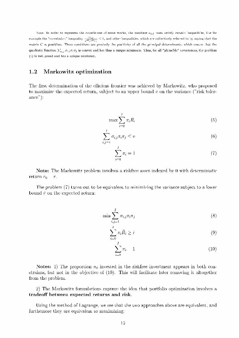
Figure 1: positively correlated stocks ( � = :5)W = (�:06; :33; :73); the small dots are the avilable stocks and the big dot represents the
portfolio recommended by the continuous approximation
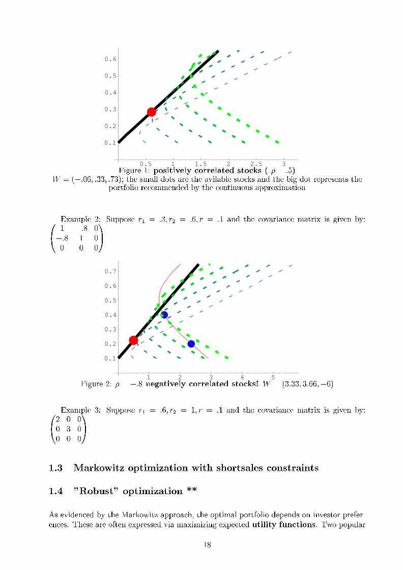
Example 2: Suppose r1 = :3; r2 = :6; r = :1 and the covariance matrix is given by:0@ 1 �:8 0
�:8 1 0
0 0 0
1A
1 2 3 4 5
0.1
0.2
0.3
0.4
0.5
0.6
0.7
Figure 2: � = �:8 negatively correlated stocks! W = (3:33; 3:66;�6)
Example 3: Suppose r1 = :6; r2 = 1; r = :1 and the covariance matrix is given by:0@2 0 0
0 3 0
0 0 0
1A
1.3 Markowitz optimization with shortsales constraints
1.4 "Robust" optimization **
As evidenced by the Markowitz approach, the optimal portfolio depends on investor prefer-
ences. These are often expressed via maximizing expected utility functions. Two popular
18

1 2 3 4 5 6 7
0.5
1
1.5
2
2.5
Figure 3: independent (uncorrelated) stocks. W = (:5; :6;�:1)
such classes of functions are: E(1+R)��1�
; which becomes in the case � = 0 ELog(1 + R) and
E e�R : When � varies, the solution of either problem will trace the same eÆcient frontier
obtained by the Markowitz approach. However, the "correct" � expressing a given investor's
preference is purely an abstract concept, which can not be determined reliably in practice.
An interesting problem raised by Sornette is to determine a point on the eÆcient frontier
which is "robust" to changes in the investor's attitudes (for example, which is within a small
distance of the optimum, for a whole range of investor's utilities). More precisely, Sornette
proposes to determine a portfolio for which both the variance and the fourth order cumulant
of the returns are small.
1.5 Exercises
Exercise 1.1
Find the minimum variance portfolio in the case of I independent risky assets.
Exercise 1.2
Find in the case of I independent risky assets the portfolio that minimizes the kurtosis
E (R � �R)4
(E (R � �R)2)2:
Exercise ** 1.3
Find in the case of I independent risky assets the portfolio that minimizes the normal-
ized cumulant of order six.
Exercise ** 1.4 Find the formula for the eÆcient frontier in the �rst example above
19

a) if no riskless investment was possible b) with the riskless investment included c) plot
both curves.
Exercise ** 1.5 Find the formula for the eÆcient frontier for two perfectly correlated
assets, if no riskless investment is possible.
Exercise ** 1.6 Find the formula for the eÆcient frontier for two perfectly uncorrelated
assets, if no riskless investment is possible
Exercise 1.7 Find the optimal investment policy for an opportunity set including a
riskless investment with rate r = 6% amd three risky assets with respective expected returns
14%; 8%; 20%; standard deviations 6%; 3%; 15% and correlations �1;2 = :5; �1;3 = :2; �2;3 = :4;
if no shortsales are allowed.
1.6 Solutions
Solution 1.1
By Lagrange's method, the solution of
minX
�2i �i;iX�i = 1
is when �i�i;i is constant; hence, �i =��1i;iPj �
�1j;j
:
20

2 Background on �nancial derivatives
In this chapter we describe some �nancial derivatives (also called options or claims), review
their history and discuss their uses.
Options are generally de�ned as contracts between two parties in which one party has
the right but not the obligation to do something at a �nal later time T , usually to buy or
sell some underlying asset ST under protected conditions. Having rights without obligations
has �nancial value, so option holders must purchase these rights, making them assets. This
assets derive their value from the primary asset ST , so they are called derivative assets. More
generally, �nancial derivatives may be viewed as random future payo�s HT which depend
somehow on the price of the primary asset, i.e. HT = f(ST ): Payment for these options
takes the form of a at, up-front sum called premium.
For example, one of the most used derivatives is the call option, which gives to the option
holder (buyer) the right to buy an asset with price St at a later "expiration" time T and
at a predecided "reserved" exercise price K. Thus, the e�ective �nal payo� to the option
holder is
HT = (ST �K)+ =
(ST �K if ST � K
0 if ST � K
(since the option will not be exercised if the asset's price drops below K).
An investor would buy a call option if he forecasts that the price at T of the asset STwill be larger than K: This could be for example a way to ensure that he can buy later
the asset (at price K), despite its increase in price. Of course, instead of buying the call
option, the investor could buy the asset in advance, but this would commit him to holding
this asset; by buying the call option (whose price is typically just a small fraction of the
asset's price), he can later give up holding the asset (if its price drops below K:) The issue
is what should be the present value of (or initial price) for such a contract. As a starting
estimate, we could assume that the price won't change, which gives the value (S0 �K)+ as
a rough approximation (since the exercise price K is only payed at expiration, this leaves
only S0 �K to be payed upfront, and this only in the case that S0 � K).
For a more sophisticated answer, we will need to incorporate somehow in our anaswer
both our view of the �nal value of St; and of "to what extent the uncertainty in whether the
option will be exercised or not" will be hedgeable.
Some of the most traded options are:
� Call options with payo� (ST �K)+
� Put options with payo� (K � ST )+
� Straddle options with payo� (K � ST )+ + (ST �K)+
� Binary, or digital options with payo� 1fST�Kg
� Spread options with payo� 1fK1�ST�K2g:
21

Note that the buyer of a call option or binary option is betting on the future price of the
stock ending above K; the buyer of a put option is betting on the price ending below K; the
straddle is a bet on movements away from K and the spread option is a bet on a precise
interval for the �nal prize. In principle, any arbitrary function HT = f(ST ) can be used
as basis for a traded option (and some are!). The �nancial interpretations of derivatives is
not important in the development of a pricing formula; this will be obtained in the greatest
generality for an arbitrary �nal payo� function HT = f(ST ):
However, the success of a certain option on the market will depend of course on the role
it plays. The put for example is very important for stock insurance. Note that the holder of
a stock share and a put will end up with the payo�
ST + (K � ST )+ = min(ST ;K)
and will thus be protected from collapses in price.
2.1 The use of �nancial derivatives
The idea of options is certainly not new. Ancient Romans, Phoenicians and Greeks traded
options against outgoing cargoes from their local seaports.
In today's world, the need to trade �nancial derivatives arises when individuals or com-
panies wish to buy an asset or commodity in advance. For instance, an airline may wish to
buy fuel in the future for a �xed price determined now, in order to avoid being subject to
price uctuations. This is also a big factor in foreign exchange. If you trade with another
country you are subject to exchange rate uctuations. By buying forward you can insure
that you can sell the product for a certain price. Thus the idea of a forward was introduced,
an agreement reached between two parties for the delivery of some commodity or stock in
the future. There are two parties to any derivatives contract, the seller and the buyer: the
buyer of the asset is said to take a long position and the seller is said to take a short position.
The trading of options is a recent phenomenon. In 1973 the Chicago Board of Trade
Options Exchange was opened for the trading of options on stocks. Prior to this individuals
who wished to purchase stock options would have to do so over-the-counter (OTC) from a
bank. The CBOT was the �rst such trading organization and there are now many places
which conduct trade in stock options. In London the option trading exchange is called
LIFFE, London International Financial Futures Exchange. You can �nd LIFFE option
prices quoted in the Financial Times.
There are three types of traders who deal with these products. Firstly the hedgers, people
who buy options as a form of insurance against adverse market movements. If you are a
company which trades with another country then you may take out an option on currency
which would pay you a certain amount if the exchange rate went heavily against you. In this
way you can hedge or protect your position to some extent by buying an option. For instance
if you import 1 billion yen worth of Japanese electronic goods and the current pound/yen
rate is 181.23, you could take out an option that will pay 1 billion yen if the exchange rate
is 200 in a years time. This means that if the cost of the yen gets too high then you can
22

cash the option and buy your goods. If the exchange rate stays low then you lose the money
spent on the option and use the exchange rate which is at a rate you are prepared to pay.
The cost of the strategy is that of buying the options and they will be reasonably cheap as
a large currency uctuation will be unlikely.
The second type are the speculators who essentially gamble on the way various assets
will move. They take a position in the market based on their beliefs and make or lose
money based on (essentially) chance. They are interested in �nancial derivatives as there
is substantial gearing. This means that it is possible to make or lose a lot more money by
buying or selling these products rather than the underlying asset. For instance a stock costs
10 pounds to buy and so you could invest 10000 pounds by buying 1000 shares. Then if the
price was 11 pounds in a years time you would have made 1000 pounds. However if you had
bought share options with a strike price of 10 pounds, then these would cost say 0.5 pounds,
so you could buy 20000. If the price went up to 11 pounds you could exercise your option,
buying 20000 shares at 10 pounds and then selling them for 11 pounds each to make a net
pro�t of 10000 pounds. Of course if the price had dropped to 9.99 you would lose all your
money!
The �nal group of traders are the arbitraguers. People who watch the market and try to
�nd situations where there are risk free pro�ts to be made. These are realized by synthesizing
a product in one market with products in another so that any price discrepancy guarantees
a pro�t. A simple example is where the price of a stock traded on two exchanges di�ers. If
a stock is trading for 100 pounds in London, for 285 D-marks in Frankfurt and the exchange
rate is 2.82 DM/$, then the price is too cheap in London. We could buy 1000 shares in
London and sell 1000 in Frankfurt and convert the D-marks into pounds to make 1063.83
pounds without any risk. These opportunities are rare and as soon as they appear are driven
out of existence by people seizing the opportunity to make money. As people buy stock the
price will increase in London and as they sell the price will decrease in Frankfurt until the
stock has the same value in the two places.
2.2 The coming of age of mathematical �nance
In 1973 there occurred also a key event in the development of �nancial mathematics, when
Myron Scholes and Fischer Black published a paper which showed how to price and "hedge"
(i.e. manage a portfolio which enables the option issuer to ful�l his obligation) the European
call option. In 1997 Scholes and Merton, who also contributed to the initial formulation of
derivative pricing theory, were awarded the Nobel prize in economics. Their theoretical work
has had a profound impact on the way the world's �nancial markets operate.
Historical note: "It was an ordinary autumn afternoon in Belmont, Mass. 1969, when Fischer Black, a 31 year old
independent �nance contractor, and Myron Scholes a 28 year old assistant professor of �nance, at MIT hit upon an idea that
would change �nancial history. Black had been working for Arthur D. Little in Cambridge, Mass., when he met a colleague
who had devised a model for pricing securities and other assets. With his Harvard Ph.D. in applied mathematics just �ve years
old, Black's interest was sparked. His colleague's model focused on stocks, so Black turned his attention to options, which were
not widely traded at the time. By 1973, the tandem team of Fischer Black and Myron Scholes had written the �rst draft of a
paper that outlined an analytic model that would determine the fair market value for European type call options on non-payout
assets. They submitted their work to the Journal of Political Economy for publication, who promptly responded by rejecting
their paper. Convinced that their ideas had merit, they sent a copy to the Review of Economics and Statistics, where it elicited
23

the same response. After making some revisions based on extensive comments from Merton Miller (Nobel Laureate from the
University of Chicago) and Eugene Fama, of the University of Chicago, they resubmitted their paper to the Journal of Political
Economy, who �nally accepted it. From the moment of its publication in 1973, the Black and Scholes Option Pricing Model
has earned a position among the most widely accepted of all �nancial models."
Black and Scholes and Merton had succeeded to price options only under an idealized
model called geometric Brownian motion market, previously proposed by the MIT economist
Samuelson. They left unanswered several important issues arising in real markets, like:
� Imperfect information (unknown mean and volatility)
� Discrete trading
� Transaction costs
In later mathematical developments, the original theory was greatly extended to answer
to these issues, the key turning out to be an approach called "martingale duality" or "risk
neutral pricing". The �rst hints at this approach came with the appearance of the Cox-Ross-
Rubinstein multinomial model, which will be discussed in section 2.
2.3 The replication of derivative contracts
The fundamental question about derivatives is what should be their premium, i.e. the value
today for a contact which will pay some function f(ST ) at a later time. How much should
people pay now for future prospects?
Example 1: Forwards Consider a forward, which is a contract to deliver a stock at
some time T in the future. One possible candidate for premium would be v0 = EST ; where E
is expectation with respect to some estimated statistical model. By the law of large numbers,
this would work alright in the long run for the seller, provided the estimated model is correct.
Sometimes the seller would win and sometimes they would lose, and this would be kind of a
"�nancial roulette" for high level bank executives.
However, this entertaining roulette is played in practice only by the buyers, since a much
more sensible strategy exists for the sellers. By charging a premium S0; they can buy the
stock now at time 0 and keep it ready for delivery until the end and thus ful�l their obligation
at time T whatever the price then. By creating what is called a hedging portfolio or
"replicating" portfolio they have eliminated any risk on their part! Clearly, if a hedging
portfolio exists, then the right price for an option should be the initial expense necessary
to set up the replicating portfolio, disregarding any possible statistical expectations ESTwe might have of the future. ( Another argument in the favor of abandoning conjectured
expectations is that if someone has strong feelings or insider info about the way St will
evolve, he might as well buy the stock itself.)
Exercise What should be the premium for a forward, if the payment is done at time T;
but decided already at time 0?
Solution: The price should still be S0er t; where r is the interest rate (assumed to be
24

constant). The reason is that the seller's hedging strategy is still to buy the stock at time 0
at the price S0 and hold it until the end, when its value would become S0er T :
Until 1973 it was considered impossible however to replicate call options and other con-
tracts, so it looked still plausible that pricing should be done by estimating some statistical
model for St, and the premium should be E f(ST ) for interest rate r = 0, or, more generally,
the present value e�r T E f(ST ) of the expected future payo�.
However, as shown in 1973 by Black and Scholes, under certain conditions de�ning an
idealized type of market called complete, the European call option could be "replicated" (or
"hedged"), by using a portfolio combining the stock and a riskless cash investment. Later,
this was shown to be true for any European option by Merton. This meant that a certain
initial premium v0 could be invested and then dynamically managed throughout time such
that the resulting "replicating" portfolio will end up with the �nal value at T which equals
exactly f(ST ) under any evolution of the prices, with no risk involved!
De�nition A replicating portfolio for an option on an asset ST with �nal payment
f(ST ) is a combination of a number of stock units �t and a loan Lt whose total value
Vt = �tSt +Lt will equal the value of the �nal claim under any evolution of the market, i.e.
VT = f(ST ):
Notes: 1) The replication of a forward involves just acquiring it initially and holding it
continuously until T; i.e. �t = 1 for any t.
2) Replicating of call options requires �guring out whether the option will end up "in
the money" (in which case we need �T = 1) or "out of the money" (in which case we need
�T = 0): Black and Scholes had found a hedging recipe which always kept some fraction
0 � �T � 1 in the stock (which re ected the current chances of ending in the money), which
could be "nudged" to end up exactly at one if ST > K and at 0 otherwise.
Black & Scholes and Merton were the �rst to show that call options may be priced
by solving the following optimization problem: construct a judiciously managed "hedging"
portfolio Wt which contains "optimally" chosen proportions of the risky asset St and of a
"riskless" cash investment with �xed interest r; in such a way that the hedging portfolio WT
ends up as close as possible to the claim at the expiration time T (i.e. WT � HT :)
In fact, Black & Scholes showed that if the evolution of the asset St could be described
by a stochastic process called geometric Brownian motion (of known volatility), and various
complications like transaction costs and constraints were ignored, then it was possible to
construct a hedging portfolio which would replicate exactly the value of the call option,
"without any risk" (i.e. WT � HT :)
The initial value W0 of the hedging portfolio provided thus in the "Brownian" world
a "no risk" initial value to be charged for a future random payment! The importance of
this "miraculous" exact "replication" was obvious from the start, both in academic and
"practitioner's" circles, who embraced the Black Scholes formula.
While the mathematics was there, it's meaning became apparent only with the intro-
duction of the Cox-Ross-Rubinstein multinomial model (1976), which is described in more
detail in Apendix A.
25
These economists considered a discrete time evolution of asset prices in which at each
possible stage the future price was restricted to take values only out of a �nite set of pos-
sibilities ("scenarios"). This brought forth the realization that these models, to be called
incomplete, did not in general allow for exact replication, except in the binomial case
when the number of future possible scenarios was restricted to 2: In this case, to be called
complete, exact hedging is possible for any type of claims HT : Completeness was thus
a result of severely restricting the stochastic model for the future (the Brownian model may
also be thought in a limiting sense, based on its "derivative" to restrict essentially the pos-
sible future scenarios to only two, one in which its "derivative" is 1 and one in which it is
�1).
Financial mathematics research focused in the beginning on the complete models. While
ignoring any type of "frictions" (incomplete information, transaction costs, etc), these models
were able to yield exact hedging and pricing solutions for a wide variety of �nancial products.
Furthemore, it turned out that the same formula, called risk neutral valuation, could be
used for the pricing of any derivative claim.
RN valuation in complete markets states that the initial value for any �nal claim
HT should be:
EQ e�rTHT
where r is the risk free interest rate of the market and Q is a measure close in some sense
to the original measure (absolutely continuous with respect to it) but having in addition
the property that under this measure the asset values have expectations which increase as if
they were riskless, i.e.
EQ St = S0ert
Furthemore, the value at any time of the optimally managed hedging portfolio should equal
the conditional expected value of the �nal claim with respect to the measure Q: (Thus
knowledge of the measure Q answers both the pricing and the hedging problem).
In the nineties, the research turned towards the more realistic incomplete models in which
exact replication is impossible and there always has to be a �nal "mishedge" WT �HT : The
seller and buyer of an option naturally disagree in their preferences on the distribution of this
mishedge and pricing is possible only after they manage to choose a joint common goal of
minimizing some "penalty" of the mishedge U(WT�HT ): Thus, hedging and pricing in incom-
plete markets amounts to solving a collection of portfolio optimization problems with arbi-
trary �nal targetHT and arbitrary objective U(x). MEMP: Minimize the expecte
minx;�
E fW0=xg U(WT �HT )
with respect to the initial investment x and the proportion � which is to be invested in the
risky asset St:
The solution of this problem, known as risk neutral valuation in incomplete mar-
kets, states that for a large class of penalty functions U(x); the solution of the optimization
problem MEMP is given by:
x = EQ e�rTHT Risk neutral valuation
where Q is the measure which is closest with respect to some "dual" distance (which depends
26

only on the penalty U) to the estimated measure P of the underlying asset. An example
illustrating this duality is given at the end of Appendix A.
2.4 Examples of �nancial derivatives
By the RN valuation principle, every derivative product should be valuated as an expectation
of the �nal payo� with respect to some (RN) measure. We will give now a list of the types
of expectations needed to evaluate some commonly traded derivatives.
According to whether the payo� depends on the whole path of the price or on the �nal
payo� only, derivatives may be divided in path dependent or European. The particular
type of path dependent options in which the buyer is allowed to choose also the moment of
termination of the contract is called American options.
Examples of European options
� Digital options with payo� 1fST�Kg
� Asset or nothing options with payo� ST1fST�Kg Call options with payo� (ST �K)+
� Put options with payo� (K � ST )+
� Butter y options with payo� N 1fK� 12N
�ST�K+ 12N
g:
where ST is the value of the stock at the "expiration" time of the contract T and K is the
"exercise" price. Note that the buyer of a call option or binary option is betting on the
future price of the stock ending above K; the buyer of a put option is betting on the price
ending below K; and the buyer of a butter y option is betting on a precise interval for the
�nal prize.
Analytical valuation of European options requires the availability of formulas for the Q
distributions of the stock process at a �xed time.
Examples of Barrier options
� Perpetual down and out digital with payo� 1fL�St;8t20;Tg
� Perpetual double barrier digital with payo� 1fL�St�U;8t20;Tg
� Down and out Call with payo� (ST �K)+1fL�St;8t20;Tg
� Double barrier call with payo� (ST �K)+1fL�St�U;8t20;Tg
where L;U are �xed barriers.
Analytical valuation of barrier options requires the availability of formulas for the Q
probability of reaching a barrier (for perpetual options) and of the Q distribution at a �xed
time of the "absorbed" stock process (for �xed period options).
Examples of American options
27

� Perpetual American put with payo� (K � S� )+ Down and out American call
with payo� (S� �K)+1fL�St;8t20;�g
where � denotes a stopping time.
The analytical valuation of American options requires the availability of formulas for the
distribution of hitting times and also that of the joint distribution of the hitting times and
the hitting position.
28

3 Risk neutral valuation in the Cox-Ross-Rubinsteinmodel
Paradoxically, the Black Scholes solution of the hedging problem was �rst provided under
a quite complex mathematical model for asset prices evolution, the exponential Brownian
motion model. This solution contained an enticing, though clearly unrealistic feature: the
possibility under the exponential Brownian motion model to hedge options exactly, with
no risk to the seller.
Puzzled by this feature, several prominent economists discussed at a conference in 1976
the "mystery" behind this exact hedging, and came up with a much simpler approach and
pricing formula.
They considered a discrete model with �nitely many scenarios allowed at each stage,
known nowadays as the Cox-Ross-Rubinstein model. The conclusion was that perfect hedg-
ing was possible only if the number of future scenarios allowed at each stage was restricted
to two (the "binomial" model), and ceased to be true for more then two scenarios. In the
latter more realistic case, several di�erent solutions of the problem were possible, depending
on the objective chosen for hedging; a "seller" hedging, a "buyer" hedging, a least squres
hedging, etc. could be de�ned.
Thus, the only multinomial markets in which perfect hedging is possible are binomial;
this type of markets are called complete and for some reason to be discussed later, the
Brownian motion model is complete just like the binomial model, even though the number
of future possible states it allows after any time interval is in�nite!
In this section we present the hedging of options under the discrete Cox-Ross-Rubinstein
model. We will consider four di�erent optimal hedging problems: the binomial (two scenar-
ios) problem, the seller problem, the buyer problem and a least squares hedging problem,
and show that in all four cases the initial value of the hedging portfolio may be computed
via a recipe to be called risk neutral valuation). This states that the value of the optimal
hedging portfolio corresponding to the various types of possible objectives can always be
expressed as an expectation with respect to a certain type of measures called risk neutral.
In this simple context it will be clear that risk neutral valuation is just a particular case
of the "strong duality theorem" of linear programming.
3.1 Hedging in discrete models
Let us denote by s0 the initial price of a stock and by S its value after one time period.
In the Cox-Ross-Rubinstein model it is assumed that S can only take values out of a
�nite set of possible values: for example, think of three possible "most likely" scenarios one
in which the stock moves to a higher value su; one in which it moves to a lower value sd and
one in which it moves to a middle value sm:
Our market also contains a �nancial derivative (option). This is a contract ("claim")
which upon expiration ensures that its holder receives a payment H whose value depends
29
(is contingent) on that of the stock: the payo� at the end of the period is either hu; hd or
hm depending on whether the stock price went up, down or to the middle value. We would
like to �nd a reasonable initial price which the buyer of this �nancial derivative should pay
to its seller at the beginning of the period.
Of course, for practical applications it is very important to decide how many possible
scenarios to use and what future values to predict for the stock value. We will ignore these
practical issues however; we will assume that �xed values su; sd; sm are given (maybe enforced
by law!) and we will focus on the mathematical consequences of this for pricing the option.
De�nition: A hedging portfolio is a combination of a number ' of stock units and
a cash investment (or loan) (to be acquired by the seller) whose total combined value at
the expiration time T is designed to be "as close" as possible to the value of the claim.
The initial value of the hedging portfolio, which is:
v0 = 's0 +
is then a quite reasonable price to be charged to the buyer. Usually the cash investment
is negative, and is thus a loan; it allows the seller to buy a larger number of stock units than
could have been bought without using it.
To emphasize ideas, we assume at �rst the interest rate to be r = 0: In this case, the
value of the loan remains unchanged and the value of the hedging portfolio at the end of the
period will be
V = 'S +
(where S is the random value of the stock). We'll call this the value evolution equation.
Sometimes, it is convenient to eliminate the loan from this expression by using the
equation: = v0 � 's0: Plugging this in (4.3.2) leads to the equivalent form:
V = v0 + '(S � s0)
also called the capital gains equation since the value of the portfolio after one period is
expressed as the sum of the initial value and the "capital gains" term '(S � s0): Thus, our
purpose is to choose the hedging portfolio ('; ) so that V will be close as possible to H in
some sense (yet to be de�ned).
V = v0 + '(S � s0) � H (15)
Sometimes we write instead of (15)
v0 + '(sw � s0) � hw
where w stands for either of the possible scenarios ("up", "down", etc).
Note that the exact equality of H and V would require satisfying k equations, where k
is the number of possible scenarios for the stock's evolution, and that we only have at our
30

disposal two unknowns ('; ) (or ('; v0): We could try to satisfy the k equations in a least
squares sense, but this is by no means the only choice. For this reason, we will consider
�rst a "toy" model in which k = 2 which allows one to determine the portfolio ('; ) in a
clearcut manner.
3.2 The one period binomial model
In this section we assume that at the end of the period the stock
may only move to one out of two values su; sd.
Under this assumption it is possible to satisfy the hedging equations exactly, whatever
happens to the stock price! Indeed, at the end of the period, the value of the hedging portfolio
and the claim are respectively
Hedge Claimvu = v0 + '(su � s0) huvd = v0 + '(sd � s0) hd
We need to solve thus a system with two equations and two unknowns:
v0 + '(su � s0) = hu (16)
v0 + '(sd � s0) = hd (17)
The system (17) is of course quite easy to solve. We will emphasize however the method
of reduction which eliminates the variable ' from the left hand side; for this we employ two
row multipliers for the equations (also called in linear programming dual variables) qu; qd;
chosen so that the coeÆcient of ' vanishes. Thus, qu; qd must satisfy
qu(su � s0) + qd(sd � s0) = 0 (18)
We also assume for conveniency that the multipliers satisfy
qu + qd = 1;
which also allows us to view them as probabilities (at least if they are positive). The
implication of these two restrictions on the row multipliers is that when combining the
equations we get a formula for the initial value v0 :
v0 = quhu + qdhd (19)
This equation has the nice interpretation that the initial value which makes hedging exact
is an average of the possible values of the �nal claim H with respect to an "arti�cial" set of
probabilities Q = (qu; qd) (yet to be determined).
v0 = EQH
31

We call Q a set of "arti�cial" probabilities, since it does not re ect any observed frequen-
cies; basically, it represents a way of expressing the result of our optimal hedging problem.
Moreover, the equation for the arti�cial probabilities (18) may be rewritten as
qusu + qdsd = s0 (20)
which has also an interesting interpretation: the "Q" expectation of the stock price after one
period equals precisely its initial value.
EQS1 = s0 (21)
De�nition: A measure (i.e. set of probabilities) Q satisfying the equation (21) is called
a risk neutral measure or "balancing" measure for the stock price.
One point left uncleared is whether the numbers (qu; qd) are positive.
Solving the system
qusu + qdsd = s0
qu + qd = 1
we �nd that
qu =s0 � sd
su � sd
qd =su � s0
su � sd
and so both (qu; qd) are positive i� sd < s0 < su: However, models not satisfying this
condition are not interesting, because they allow arbitrage which means the possibility of
in�nite pro�ts: indeed, if both s0 < sd < su a hedging portfolio with ' = 1 would reap
in�nite pro�ts and the same would be true by shortselling ' = �1 in the case sd < su < s0:
In conclusion, we obtained for the binomial model the
Theorem 3.1. Risk neutral valuation theorem: Under the assumption of noarbitragesd < s0 < su; the initial value which makes perfect hedging possible may be expressed as anexpectation EQH of the �nal claim with respect to the (unique) risk neutral measure Q:
Note: In this simple case, the original hedging problem of �nding '; may anyway be
solved directly quite easily, yielding
' =hu � hd
su � sd; =
hdsu � husd
su � sd
However, in more complicated situations, risk neutral valuation (i.e. the determination
�rst of the measure Q comprised of the row multipliers) becomes by far the easiest method
for determining the initial value and the hedging strategy.
32

Exercise: Develop the CRR model with non zero interest rate r, over a period
of length t:
Solution In the general binomial case when the interest rate r is non zero, the (perfect)
hedging equations become:
' su + ert = hu
' sd + ert = hd
After eliminating from the initial condition = v0 � 's0 we get the capital gains
equations:
v0er + '(su � s0e
rt) = hu
v0er + '(sd � s0e
rt) = hd
The balancing equations for the dual multipliers qu; qd are now qu + qd = 1 and qu(su �s0e
rt) + qd(sd � s0ert) = 0 or
EQS1 = s0ert (22)
whose interpretation is that qu; qd are probabilities under which the expected value of the
stock after time t grows by ert:We call such probabilities Q = (qu; qd) a risk neutral measure
for the stock price. Their values are:
qu =s0e
rt � sd
su � sd
qd =su � s0e
rt
su � sd
Combining the capital gains equation we �nd that v0ert = quhu + qdhd: The initial value
now has to equal the discounted value of the �nal claim with respect to the risk neutral
measure.
v0 =quhu + qdhd
ert= e�rtEQH
The optimal number of stock units is unchanged ' = hu�hdsu�sd and the optimal loan is given
by: ert = hdsu�husdsu�sd :
In conclusion, for any interest rate r; if the future would consist only in one out of
two possible states, there would exists a unique risk neutral measure and an exact hedging
strategy would be possible. By charging an initial payment v0 which equals the discounted
value of the �nal claim with respect to the risk neutral measure, and investing it as
indicated, the seller of any derivative product could ensure that he can pay it o� without
any risk. Hence the price for the derivative must be v0 = e�rtEQH. Any other price would
allow arbitrage as one could use the optimal hedging strategy, either buying or selling the
derivative, and make guaranteed pro�ts.
33

3.3 Connecting the binomial and exponential Brownian motionmodels
The Black Scholes formula v0 = E�e�rTh(ST ) for valuing derivatives under the exponential
Brownian motion model ST = s0e�T+�BT by adjusting the drift of the exponent to r �
�2
2is derived under a speci�c continuous model, and under the asssumption of continuous
rebalancing of the hedging portfolio (at no transaction costs).
At the opposite end, the binomial pricing formula is derived under the assumption of no
intermediate trading, but by assuming that the stock can only move at the end of the period
to one of two values.
Initially, we would guess that the prices produced by these two completely unrelated
models should be quite di�erent. However, this is not so, provided that the two values of
the binomial distribution are judiciously chosen to approximate the distribution of ST =
s0e�T+�BT : Below, we will use the approximation:
"Discrete approximation for Brownian motion": If an asset evolves as exponential
Brownian motion ST = s0e�T+�BT ; a good two value approximation for its �nal value is :
su; sd = s0e��
pT ;
i.e. the exponent �T + �BT is approximated by ZT = ��pT with equal probability, inde-
pendently of �.
Note: If the Brownian motion XT appearing in the exponent had no drift (thus XT =
�BT ), the natural two value approximation would be of courseXT � ��pT ; because the two
valued distribution taking the values ��pT with equal probability is the only symmetric two
valued distribution which has the same mean and variance as the original model XT = �BT :
When XT has drift, we could still keep these two values and adjust their probabilities to �t
the drift by the formula p; q = 12(1� �
�2D): However, the drift of the exponential Brownian
motion model and the probabilities p; q end up thrown to the garbage anyway in the pricing
process, so it is natural to disregard them from the beginning and use always the same
approximation as if there was no drift!
Example 1 Let us �nd the price of a call option and a put option if S0 = 6;K = 5; � =
:2; r = :05 and t = 2 years, both under the Black Scholes and under the binomial model
based on the "discrete approximation for Brownian motion".
The table below gives the Black Scholes call value, the binomial call value, the Black
Scholes put value and the binomial put value, for 24 times, starting with 8 months=2/3 year
and ending with 16 years. The last two columns computed as a check C � P + ~K for both
models; as required by put call parity, that equals precisely S0 = 6: Our answer is in the
third row. Amazingly, the two models produce quite close �gures, of 1:60 and 1:64; for the
call. Note that in the beginning the values are quite close to the 0 volatility lower bound
S0 � K = 1; and as the time increases they get closer to the upper bound S0 = 6 (which
corresponds to 1 volatility ).
34

1.202 1.164 0.0382 0 6. 6.1.41 1.413 0.0872 0.0909 6. 6.1.598 1.643 0.1224 0.1673 6. 6.1.771 1.84 0.1473 0.2154 6. 6.1.933 2.013 0.1649 0.2457 6. 6.2.084 2.17 0.1773 0.2636 6. 6.2.226 2.313 0.1858 0.2725 6. 6.2.362 2.445 0.1912 0.2747 6. 6.2.49 2.567 0.1944 0.2716 6. 6.2.613 2.682 0.1958 0.2643 6. 6.2.731 2.789 0.1958 0.2537 6. 6.2.843 2.889 0.1947 0.2406 6. 6.2.951 2.984 0.1927 0.2253 6. 6.3.055 3.073 0.1901 0.2083 6. 6.3.154 3.157 0.1868 0.19 6. 6.3.25 3.237 0.1832 0.1706 6. 6.3.342 3.313 0.1792 0.1505 6. 6.3.431 3.386 0.175 0.1297 6. 6.3.516 3.454 0.1706 0.1085 6. 6.3.599 3.52 0.166 0.0869 6. 6.3.678 3.582 0.1614 0.0652 6. 6.3.755 3.642 0.1567 0.0434 6. 6.3.829 3.699 0.152 0.0216 6. 6.3.901 3.753 0.1474 0. 6. 6.
2.268 2.081 2.096 2.0482.973 2.75 2.731 2.6863.465 3.235 3.198 3.1663.838 3.615 3.569 3.5524.132 3.923 3.873 3.8724.371 4.18 4.128 4.1424.567 4.395 4.346 4.3724.731 4.579 4.532 4.574.869 4.737 4.693 4.7424.986 4.874 4.834 4.8915.087 4.992 4.957 5.025.173 5.096 5.065 5.1345.249 5.187 5.16 5.2345.315 5.267 5.245 5.3215.372 5.338 5.321 5.3985.423 5.4 5.388 5.4665.468 5.456 5.447 5.5265.509 5.506 5.5 5.5795.544 5.55 5.548 5.6265.577 5.59 5.591 5.6675.606 5.625 5.629 5.7045.632 5.657 5.663 5.7375.655 5.686 5.694 5.7655.677 5.712 5.721 5.791
Example 2 Let us �nd the price of the same call option under the Black Scholes and
under the binomial model, if � = :4
The table above gives �rst the binomial price, then two other approximations discussed
in the next section, and �nally the Black Scholes price, for 24 periods starting with two years
and ending with 48 years. We note �rst that for large times, the values get very close to the
upper bound S0:
We note also that all four models produce close results; however, these are far from
the previous ones obtained when we estimated the volatility to be :2: In conclusion, the
estimated volatility has a bigger impact on the price than the model we use.
The volatility of a process is estimated from the equation �2NY
=PN
i=1(log(Si+1� logSi)2; where N is the total number
of observations and Y is the number of trading days per year (so that NY
is the total time observed).
This is however only past observed volatility. The main issue of option pricing is not the
model used, but the forecasting: what will be the future volatility be?
35

In the next section we will show how we can improve on the binomial model by allowing
several intermediate "review" times at which the portfolio may be rebalanced.
3.4 The multiperiod binomial model
We will re�ne now the two valued approximation of the Brownian motion from the previous
section to the natural situation when we observe the process a �nite number of times situated
at intervals t1; t2; ::::; tn; whereP
i ti = t:
At each step, we use the "discrete approximation for Brownian motion"
dXti � ��pti:
This results in the following pricing method, which is best performed organizing the
computations as a tree.
The multiperiod binomial model:
1. For each i = 1; :::; n we compute the number ri = rti; the two price multipliers ui; di =
e��pti and the two risk neutral probabilities
pi =eri � di
ui � di; qi =
ui � eri
ui � di
2. For each branch of the tree, we compute the risk neutral probability qw by multiplying
all the probabilities along the branch, the �nal asset price sw and the �nal claim hw:
3. We evaluate the risk neutral expectation:
v0 = e�rtEQH = e�rtX
qwhw
Exercise 3: Suppose that two "review" stages of :75t; :25t are chosen for hedging
the call option of example 2: Using the multiperiod binomial model, �nd the risk neutral
probabilities at each stage and the initial value which makes exact hedging possible. Ans:
See table 2.
Exercise 4: Redo exercise 3, if the interest rate over the �rst period is r1 = :1 and over
the second period it is r2 = 0:
Conclusion: If enough review stages are chosen, the multiperiod binomial model is
essentially identical to the Brownian motion model, and has the extra exibility of allowing
the introduction of additional features speci�c to each stage.
Note: It may be shown by induction that the multiperiod binomial method hedges exactly any claim (in this model,the number of possible distinct �nal future states is 2n; but we also have 2n decision variables, one for each branch of the tree)!
We explain now how perfect hedging works, by "backwards induction" (also called dynamic programming). Consider an
option with expiry in n periods (for concreteness, say n = 2:) At expiry, "nature" can be in any of 2n states with corresponding
payo�s hw : Our recipe for perfect hedging over one step speci�es the necessary value for the hedging portfolio at time n � 1;
36

this necessary value maybe viewed as a claim at time n� 1; to hedge this, we will need a certain value at time n� 2; etc. In
conclusion, we will need to �nd the "necessary" value at time t vt; this function will be entirely determined by the value of the
stock at time t; i.e. vt = v(St):
If we allow in our toy model more than two possible values for the future evolution
of the stock price, clearly perfect hedging ceases to be possible. Also, the risk neutral
measure (balancing probability) ceases to be unique (since we still have only two equations
to determine it, but more variables qw: Instead, there is a whole set of balancing probabilities,
which yield di�erent expectations for the �nal claim EQH(ST ): Which one should one use?
The answer to this puzzle is that all these risk neutral expectations provide reasonable
initial prices, in that that they and only they eliminate the possibility of arbitrage. Furthe-
more, each of these potential initial prices corresponds to a certain optimization objective,
which expresses the seller's and buyer's attitudes towards the "mishedge" (the hedging er-
ror). In conclusion, the set of all possible RN measures gives rise now to a con�dence band
of RN prices
infQ
EQH(ST ) � supQ
EQH(ST )
rather than to a unique price.
Any choice within this risk neutral band of prices is now possible. We illustrate this
in the next sections, where we show that the highest possible price coincides with the price
which the seller would like to impose (so that he incurs no risk) while the lower price is the
price which would eliminate the buyer's risk, while compromise attitudes like minimizing the
least squares of the mishedge error lead to prices in between.
3.5 Super and sub replicating in multinomial models
The buyer and the seller of a derivative contract have di�erent opinions about what is a fair
price; the �rst can agree only to "subreplicating" portfolios (see below) while the other can
agree only to "superreplicating" portfolios.
Consider now a market in which a stock with current value s0 can move after one period
to any of a �nite set of possible values sw: To preclude arbitrage, we need to assume that
the value of the stock can go both above and below s0: A bank sells a �nancial derivative
which will pay hw in the case when the value of the stock becomes sw: The seller would like
to charge the buyer a certain price v(S)0 which has to be enough to allow him to create a
"hedging" portfolio whose value will surely end up higher than the derivative (thus
allowing him to provide it). This is achieved by buying some number ' of stock units. The
value of the hedging portfolio after one period is again given by the capital gains equation
v0 + '(sw � s0): The seller's pricing problem is to chose '; v(S)0 which solve the linear
programming problem
min v(S)0 subject to
v(S)0 + '(sw � s0) � hw for any event w
The seller's pricing problem expresses the seller's wish to price as cheaply as possible his
product, under the constraint that the the value of the hedging portfolio at time 1 will allow
37
him to pay the claim with no risk.
Similarly, the buyer's pricing problem is:
max v(B)0 subject to
v(B)0 + '(sw � s0) � hw for any event w
The buyer's pricing problem expresses the buyer's agreement to pay for the claim as
much as possible, as long as he is absolutely sure that the seller's hedging portfolio can never
exceed the claim.
Exercise: Consider a one period market with three values and interest rate r = 0:
Assume three possible future scenarios, with claim values hu = 9; hm = 6; hd = 1; depending
on whether the price of the stock goes from s0 = 2 to su = 3; sm = 1:5; sd = 1:
a) Plot on a S;H(S) graph the three possible scenarios.
b) Note that the seller's problem of �nding '; so that +'sw � hw may be interpreted
as looking for the line which is above all the three points, and which has the lowest intercept
over S = s0: Similarly, the buyer's problem of �nding '; so that + 'sw � hw may be
interpreted as looking for the highest line which is above all the three points and has the
highest intercept over S = s0:. Determine these lines, �rst graphically and then symbolically
(i.e. �nd the hedging formulas for '; preferred by the seller and the buyer, respectively.
b) Find the initial prices recommended by the seller and buyer. Is the market complete,
i.e. is the buyer price equal to the seller price?
c) Show that the seller and buyer's initial prices can both be expressed as expectations
of the claim values with respect to certain risk neutral measures (to be determined).
Solution
a) We �nd graphically that the seller is concerned about the middle and upper cases,
while the buyer is concerened by the extreme cases. The formulas for '; are found by
plugging in the formulas from the binomial section ' = hu�hdsu�sd ; = hdsu�husd
su�sd the respective
cases.
b) Using the formula v0 = 's0 + we �nd that the seller's price is 7 and the buyer's
price is 5: The market is incomplete.
c) The two risk neutral measures of the seller/buyer, obtained by plugging the respective
38

values in the formulas from the binomial section
qu =s0 � sd
su � sd; qd =
su � s0
su � sd
are qu = 1=3; qm = 2=3; qd = 0 and qu = 1=2; qm = 0; qd = 1=2.
One way out of the seller-buyer con ict by using the regression line of the points above
will be given in the next section.
3.6 Choosing among several risk neutral measures **
To resolve the buyer-seller con ict which is due to the impossibility of perfect hedging, we
have to introduce some speci�c minimization criterion for the "mishedge" (i.e. the di�erence
between the claim and the �nal value of the hedging portfolio).
One possibility is to choose to minimize the expected value of the square of the "mishedge."
Other reasonable choices are powers, exponentials, logarithms and they are referred to as
utility functions. With the quadratic utility we are thus led to the optimization problem:
minv0;'
E (H � v0 � '(S � s0))2 =
Xw
pw(hw � v0 � '(sw � s0)2 (23)
Notes 1) In this objective we see for the �rst time appearing the estimated probabilities
pw of the various scenarios.
2) The least squares objective is a compromse which keeps in check both the buyer's and
seller's ambitions (who have the con icting aspirations to make the above di�erence positive
and negative, respectively).
(23) is a classical regression problem (of the vector H on the vector dS = S � s0 and on
a vector of ones �1). The well known solution is
' =Cov (H; dS)
V ar(dS)
v0 = EH � 'E dS:
Letting � = E (dS); �2 = V ar(dS) denote the mean and variance of the change in the
stocks price (with respect to the estimated measure P = (pw); and plugging Cov (H; dS) =
E [H(dS � �)] we �nd that v0 simpli�es to
v0 = (1 +�2
�2)EH � �
�2E [H dS] =
Xw
hwqw
where qw = pw(1 +�2
�2� �
�2(sw � s0)); which can again be interpreted as an expectation.
Theorem 3.2. The initial value v0 which leads to the optimal hedging of the claim in leastsquares sense is given by
v0 = EQH
39

where the measure Q is given by qw = pw(1 +�2
�2� �
�2(sw � s0)).
The measure Q has total mass 1 is risk neutral (but unfortunately may have negativecomponents qw).
Exercise: Check the last statement.
Solution It is easy to check thatP
w qw = 1 + �2
�2� �
�2E [dS] = 1:
Also, Q is risk neutral:P
w qw(sw�s0) = (1+ �2
�2)E [dS]� �
�2E ([dS]2) = �(1+ �2
�2� �2+�2
�2) =
0
40
Note: It is also possible to derive the same RN measure by minimizingP
w pw
�qwpw
�2over the set of all RN measures.
Namely, letting zw = qwpw
; where pw; qw are the "real world" and rsik neutral probabilities for the stock, we are looking for
a solution of the "dual" problem
minQ
EP (dQ
dP)2 = min
Xw
pwz2w
Xw
pwzw(sw � s0) = 0
Xw
pwzw = 1
Note that if we drop the �rst constraint, the solution of the remaining problem would be zw = 1;, i.e. Q = P itself.The dual problem can thus be interpreted as trying to �nd a measure which is as close as possible to the observed P (ina quadratic sense) and which is also risk neutral. It was later shown by Karatzas, Lehoczky, Shreve and Xu(1991) and byKramkov and Schachermayer(1998) that to any possible "utility" (penalty) function of the mishedge (like the quadratic here)there corresponds a unique appropriate "dual" distance between Q and P which needs to be minimized.
Exercise: Solve the dual minimization problem for zw:
Solution: By the method of Lagrange multipliers the solution must be of the form zw = k1(sw � s0) + k2; we �nd that
k1 = � �
�2; k2 = 1 + �2
�2where � = E(S � s0); �
2 = V ar(S � s0):
41

4 Stochastic models in �nance
Stochastic processes are crucial for the understanding of modern �nance and insurance. They
are immensely useful and have become the common language of workers in many apparently
unrelated areas like �nance, physics and social sciences, connected only by their common
interest of untangling as time passes of the predictable from the uncertain in the unfolding
of future events.
In this section we will visit brie y the most frequently used stochastic processes in math-
ematical �nance and mention some problems where they are used. We will introduce �rst
two general families of processes:
� Levy (or additive) processes, which are sums of identical independent summands, and
� multiplicative processes which are products of identical independent factors.
Finally, we will discuss the favorite process in mathematical �nance, exponential Brow-
nian motion and some applications.
4.1 Levy (additive) processes
4.1.1 Random walks
These are processes of the form
ST =
TXt=1
Xt
where Xt are i.i.d. (independent identically distributed) random variables. In the case when
Xt = �1 the process (4.1.1) is called a simple random walk.
When the probabilities of going right or left are both equal to w:p::5 we have a symmetric
random walk and if we allow unequal probabilities p 6= q for moving right and left we have
a biased random walk.
4.1.2 Compound Poisson processes
In continuous time, we generalize by allowing our process to jump after arbitrary intervals of
time ti: Letting NT denote the total number of jumps which occurred in the interval [0; T ];
we consider thus processes of the form:
ST =
NTXt=1
Xt
42

In order for this process to be Markovian it is necessary to assume that the interarrival
times Ti are exponentially distributed, which is equivalent to the counting process NT being
a Poisson process. In this case we call the process (4.1.4) a compound Poisson process or
a pure jump process.
4.1.3 Levy processes
Random walks and compound Poisson processes have both the property that there incre-
ments over disjoint time intervals are independent, with a distribution which depends only
on the length of the time interval (and not on its starting point).
Levy processes are de�ned as the family of all processes satisfying the conditions above.
Thus:
De�nition 4.1. A Levy process is any process Yt for which:
� The increment Yt � Ys of a Levy process over an interval [s; t] is independent of theincrement over any other time interval disjoint from [s; t]:
� The distribution of the increment Ys+t�Ys is the same as that of the initial incrementof time length t. i.e. Yt � Y0; independently of s:
Brie y, we say that a Levy process has stationary, independent increments.
As noted, both ransom walks and compound Poisson processes satisfy these properties.
The same is true about linear deterministic motion rt:
The exercises below will show that �rst moments, variances as well as cumulant generating
functions (to be de�ned below) of Levy processes increase linearly with time (in this sense,
we may think of Levy processes as "linear" random processes).
They are based on the following calculus lemma:
Lemma 4.2. If a continuous function f(t) satis�es for any s; t; the identity:
f(t+ s) = f(t) + f(s)
then f(t) must be a linear function, and so f(t) = f(1)t:
Exercise 4.1 Show that if Yt is a Levy process, than at any time t we have:
a) m(t) = EYt = tEY1
b) v(t) = VarYt = tVarY1
c) Establish a), b) directly (without using Lemma 1) for integer times t:
Exercise 4.2 Show that the the moment generating function of any Levy process YtM(u; t) = E euYt satis�es the identity M(u; t + s) = M(u; t) M(u; s): Conclude that M(u; t)
is of the form M(u; t) = etc(u).
43

The function
c(u) =log(E euYt )
t
is called cumulant generating functional.
Note: The cumulant generating functional of a Levy process characterizes uniquely the
process (since the moment generating function does) and is typically easier to compute than
the density.
In the next exercise we obtain formulas for the expectation, variance and cumulant gen-
erating functional of a compound Poisson process St (with bounded jumps) whose jumps'
density is f(x):
Exercise 4.3 a) Show that ES1 ; VarS1 for a compound Poisson process are given by:
ES1 = �EX1
VarS1 = �E (X1)2
b) Compute the moment generating function E e�St compound Poisson process St (as-
suming bounded jumps) and show that c(�) is given by:
c(�) = �(MX1(�)� 1) = �(
Z 1
0
e�xf(x)dx� 1) (24)
Another simple type of continuous time Levy process is obtained by adding together a
deterministic linear trend pt and a compound Poisson process ST =PNT
t=1Xt:
YT = pT + ST
Except for allowing both negative and positive jumps, the model (4.1.3) above is precisely
the classical model of the reserves of an insurance company.
4.1.4 Application: Insurance premia
The aggregate claims process for an insurance company over a �xed time interval T is
modeled by a compound Poisson process
ST =
NTXt=1
Xt
We list below a couple of proposed recipes for determining insurance premia. We denote
by p the premium per year. Then , the premium per T years pT may be computed from:
1. The mean value principle
44

pT = (1 + �)EST
by which the company tries to cover its claims, with an extra "safety" factor of �:
2. The variance principle
pT = EST +�
2VarST
by which the company makes its extra safety charge proportional to the variance (which
maybe viewed as a measure of the risks incurred). The factor � is called risk tolerance.
3. The exponential principle
p =c(�)
�
We will see in Exercise 4 below that the exponential and variance principles are very
close to each other for small � (the variance premium and the two terms Taylor expansion
around � � 0 of the exponential premium coincide).
Exercise 4.4 Let c(u; t) denote the cumulant generating functional of a general stochas-
tic process Xt, de�ned by the equation E e�Xt = ec(�;t). Derive formally the Taylor expansion
c(�; t) = � EXt +�2
2VarXt + :::
Conclude that the two terms Taylor approximation for the exponential premium c(�)
�of
a compound Poisson process St is given by:
c(�)
�= ES1 +
�
2VarS1 + ::: = �(EX1 +
�
2EX2
1 )
The importance of the expectation principle is provided by its connection to the so called
"ruin probability" described in the next theorem, which will be established in a future section.
Theorem 4.3. (Lundberg's approximation) Let Ut = u+ pt�St denote the reserves processof an insurance company with inital reserves u and premium rate p: Let '(u) denote theruin probability, i.e. the probability that Ut ever becomes negative
'(u) = PufUt � 0; for some t > 0g
Then, for any � > 0; choosing the premium rate by the exponential principle p = c(�)
�ensures
that the ruin probability is exponentially small with asymptotic rate decay �; i.e.
'(u) � e��u
The concern for having a large rate of decay � and thus a small ruin probability re ects
a conservative point of view: a concern with an event of small probability but catastrophic
consequences.
45

Note: In practical computations � is very small and thus it is alright to replace the
exponential principle by its variance approximation:
c(�)
�= �(EX1 +
�
2EX2
1 )
In conclusion, �nding insurance premia is based on computing expectations, variances,
or cumulant generating functions of a Levy process. The last principle is supported by
important conservative concerns; for small � however the variance principle which requires
less estimation provides a very good approximation.
The linearity of all the above premia in time (a desirable property for a pricing principle)
was ensured by linearity properties of Levy processes established in Exercises 1-3.
4.1.5 Brownian motion
The class of Levy processes includes one more types of process: Brownian motion, which
maybe obtained as a limit of the symmetric and biased random walks discussed in a previous
section.
Historical note:
Brownian motion was �rst introduced by Einstein to model the motion of pollen particles in asuspension, under the impact of collisions from electrons. In one dimension, this movement maybe modeled as a sum of small jumps �D (think of D as of the average movement of the pollenparticle to the right or left), which occur after very smalll time intervals of h: In a �xed interval oftime t there will be about n = t=h jumps, and so the total movement will be Sn =
Pni=1Xi:
Einstein realized that in order to obtain a �nite limit as h;D ! 0 this quantities had to berelated to each other. Indeed, computing the variance of Sn we �nd:
VarSn = nVarX1 = nEX21 =
t
hD2
and thus to get a �nite limit for �xed t we need to assume that D2 � kh for some constant k:
Using this relation (called Einstein scaling) Einstein was able to compute accurately the Avogadro
number, which is related to k: Since k depends on the chosen units of length and time, we will
mostly ignore it (take it as 1).
We assume thus the Einstein scaling D =pt and de�ne Brownian motion Bt as the
limit when h;D ! 0 of the random walk described above. Brownian motion is only a
mathematical idealization. In real life, we can only observe random walk. However, this
continuous limit turns out to be more convenient when doing analytical computations than
the "real life" random walk.
Note that as both h;D ! 0; the jumps of the random walk are small, but still quite large
when compared to the time interval. Thus, Brownian motion is a continuous model for a
sum of very frequent quite large shocks which can go equally up or down.
De�nition 4.4. Let Sh(t) =Pbt=hc
i=1 Xi denote a symmetric random walk with increments
Xi = �D with probabilities 1=2; and occurring after time intervals of h; where D =ph
and bt=hc denotes integer part.
46

Standard Brownian motion is the limit of symmetric random walks:
Bt = limh!0
Sh(t)
Theorem 4.5. Standard Brownian motion B(t) is characterized by the following three prop-erties:
1. B(t) has a Gaussian distribution with mean 0 and variance t: Its density is thus:exp (� x2
2 t)p
2� t:
2. It is a Levy process: thus it has stationary increments ( meaning that B(t) � B(s)has the same distribution as B(t� s)), and increments over disjoint time intervals areindependent.
3. Brownian motion has continuous paths
Proof of 1:
1. The Gaussian distribution is a consequence of Bt being a sum of in�nitely many
small shocks (by the central limit theorem which states that sums of i.i.d's have a nearly
Gaussian distribution). Formally, we need to check that the �rst and second moments of
the process Sh(t) converge to those of the Gaussian distribution prescribed (exp (� x2
2 t)p
2� t), which
has mean 0 and variance=second moment t: Indeed, it is easy to check that the mean of
Sh(t) = 0 equals 0 and the variance of Sh(t) is n D2 = bt=hc h! t:
Thus, by the central limit theorem it follows that the limiting distribution of Sh(t) has
to be Gaussian with mean 0 and variance t:
Property 2 follows immediately from the corresponding property of the random walks.
Property 3 is very hard to establish and beyond the scope of these notes.
Exercise 4.5 a) Compute the moment generating function E euN of the standard normal
random variable.
b) Compute the moment generating function E euX of normal random variable with mean
0 and standard deviation �: Hint: X may be represented as X = �N:
c) Find E eu�Bt if Bt is stadard Brownian motion.
Exercise 4.6 If B(t) is standard Brownian motion, �nd EB(s)B(t) if s < t: Hint: Write
B(t) = B(s)+[B(t)�B(s)]; and use the independence of B(s) of the increment B(t)�B(s):
4.1.6 Brownian motion with drift
Adding together a deterministic trend �t and an "ampli�ed" Brownian motion �B(t) yields
the process
B�;�2(t) = � t+ �B(t)
47

called Brownian motion with drift. Note that its mean and variance at time t are
respectively:
EB�;�2 (t) = � t
VarB�;�2(t) = �2 t:
The density is thus
exp (� (x�gt)22�2 t
)p2��2 t
:
Exercise 4.7 Find the moment generating function of Brownian motion with drift
E euBg;� (t) and its cumulant generating function .
The drift parameter � will also be called growth parameter; this name is suggested by
the theorem below, a consequence of the law of large numbers, which shows that for large
times the drift dominates the oscillation part of the Brownian motion with drift.
Theorem 4.6. The long term behavior of Brownian motion with drift is:
limt!1
B�;�2(t)
t= �
By this result, we may think of Brownian motion with drift as a process which oscillates
wildly on a short time scale (due to �Bt) around a long term trend of �t:
The "real life" analog of Brownian motion is the biased random walk with vanishing
bias de�ned below.
We call a process Sh(t) a "biased random walk with vanishing bias" if it is of the form:
Sh(t) =Pn
i=1 Zi with Xi = �D with probabilities p; q = 1=2 � �2�2
D; n = bt=hc, andD;h � 0 satisfying the scaling relation D2 = �2h:
We will check now that the �rst and second moments of the process Sh(t) de�ned above
converge to those of the Brownian motion B�;�2(t): Indeed, the mean of X1 is D (p � q) =
D ��2
= h � and thus the mean of Sh(t) is n h � ! t �: Similarly, the variance of X1 is
D2 � h2�2 � h �2 and so the variance of Sn(t) is n h �2 ! t �2:
Theorem 4.7. The limit of the biased random walk with vanishing bias Sh(t) de�ned by theparameters �; � is the Brownian motion with drift corresponding to those parameters.
Note: Brownian motions are actually easier to work with than their discrete counterparts,
as far as analytic manipulations are concerned . We will see in a later section that while
working with discrete random walks requires computing sums and solving di�erence equa-
tions, working with Brownian motion requires computing integrals and solving di�erential
equations, which are somewhat easier analyically. For example, the distribution of symmet-
ric random walk at a �xed time is given by some complicated sums, while the distribution of
Brownian motion at a �xed time has a simpler formula (provided by the Gaussian density).
48

4.1.7 Classi�cation of Levy processes
We quote now an important theorem whose proof is beyond the scope of these notes, which
shows that all Levy processes are made up of three components: the deterministic trend, a
compound Poisson part and Brownian motion.
Theorem 4.8. Decomposition of Levy processes Any Levy process may be decomposedas a sum of three parts.
Yt = pt+ S(t) + �B(t)
where B(t) is standard Brownian motion. Strictly speaking, the part S(t) maybe more generalthan a compound Poisson process, in the sense that it may allow jumps to occur with in�nitefrequency in which case it is called pure jump Levy process
Note that a Levy model is characterized by three scalar parameters: �; p; � and a "func-
tion parameter", the distribution F (x) of the jumps, and is as such much richer than a
Brownian motion model, which has only two parameters: the deterministic trend p and the
volatility �:
Unlike Brownian motion, Levy processes don't usually have simple density formulas, but
they do have simple cumulant generating functions. This is illustrated in the exercise below
where we compute the cumulant generating functional for a general Levy processes.
Exercise 4.8 Using the decomposition theorem for Levy processes, show that the cu-
mulant generating functional for a Levy process whose decomposition is Yt = pt+ �Bt + Stis given by:
c(u) = pu+�2
2u2 + �
Z(euz � 1)f(z)dz
Note: Despite the fact that Brownian motion, compound Poisson processes and deter-
ministic motion are so di�erent at �rst sight, most of their properties can be expressed in a
uni�ed way by using the cumulant generating function c(u):
4.2 Multiplicative (exponential) processes
Random walks are additive processes, by which we mean that they satisfy a recursive
formula
Xt+1 = Xt + Zt+1
In �nance, in keeping with the mechanism of compounding of interest, we are also inter-
sted in multiplicative processess satisfying a recursive formula:
St+1 = StZt+1
49

where Yi are independent identically distributed random variables.
Thus, a multiplicative process is a product
St =
tYi=1
Zi
of positive factors. The decomposition above suggests the following result
Lemma 4.9. A process in discrete or continuous time is multiplicative i� its logarithm isadditive.
Thus, multiplicative processes are precisely the exponentials of Levy processes.
Example: Exponential Brownian motion (EBM) is the process
St = S0ept+�Bt
The birth of modern mathematical �nance may be traced to the adoption of the EBM
model by Samuelson, around 1960 (previous attempts around 1900 by Bachelier to model
asset evolution as Brownian motions with drift has a lesser impact).
A class of processes of great importance in �nance are the so called risk neutral pro-
cesses. Typically, we assume the existence of a deterministically increasing "riskless" invest-
ment which yields a �xed interest rate r:
De�nition: A process St is called risk neutral if its expectation increases exponentially
at rate r:
ESt = ertS0
(i.e., the expected increase equals that of the riskless investment).
Exercise 1.9 below shows that the study of risk neutral processes may be reduced to that
of the special case (obtained when r = 0) of processes with constant expectation. These
processes �gure also prominently in the theory of gambling, where they received the name
of martingales (from a certain gambling strategy).
De�nition A martingale is process which has constant expectation
ESt+s = ESt = S0
Informally, martingales are processes of "balanced" evolution, in the sense that their expected
increase and expected decrease counterbalance each other on average.
In discrete time, it is easy to see that an additive process is a martingale i� its increments
have mean 0 and a multiplicative process is a martingale i� its factors have mean 1:
Exercise 4.9 A process St is risk neutral i� the "discounted" process
~St = e�rtSt
50
is a martingale.
Note: The expectation of the discounted process E ~St = E e�rtSt plays a crucial role in
all �nancial considerations and is called present value.
Exercise 4.10
1. Find a necessary condition for a Levy process to be risk neutral.
2. Find a necessary condition for a Levy process to be a martingale.
3. Show that an exponential Levy process is risk neutral i� it satis�es the equation
c(1) = r
4. What does this condition become in the case of the exponential of Brownian motion
with drift?
5. Find a necessary condition for an exponential Levy process to be a martingale.
6. What does this condition become in the case of the exponential of Brownian motion
with drift?
It turns out that most of the time in mathematical �nance one needs only to work with
risk neutral processes and martingales.
In the following subsection we discuss the favourite model in mathematical �nance: ex-
ponential Brownian motion, which is the exponential of a Brownian motion with drift.
4.2.1 Exponential Brownian motion
A process S(t) is called exponential (geometric) Brownian motion if it is of the form
St = S0 exp (g t+ �Bt)
Exponential Brownian motion became in the seventies the preferred model for the evolu-
tion of stocks. The reason is that the discrete evolution of assets is most naturally modeled as
a multiplicative process Sn(t) = S0Qn
expYi and in the continuous time limit this converges
to geometric Brownian motion.
The parameter � is called volatility, and the parameter g is called sometimes drift and
sometimes "growth rate", because it provides (by the law of large numbers) the path behavior
of the logarithm of the process. For example, note that the law of large numbers implies
that for g > 0 we must have limt!1 St =1; and for for g < 0 we must have limt!1 St = 0:
Thus, the sign of g determines the limiting behavior of the asset.
The density of exponential brownian motion has the peculiarity that it may exhibit quite
large separation between the "mode" and the "expectation", as illustrated in the �gure
51

below. Thus, the most probable values (near the mode) are often quite smaller than the
expectation. It turns out (as a consequence of the law of large numbers) that for t large,
GBM is well approximated by egt; which turns out to equal also the median of the process.
We will show in an exercise below that the expectation of geometric Brownian motion is
given by e(g+�2=2)t; the mode is only e(g��
2=2)t; with the median egt in between.
1 2 3 4 5 6
0.05
0.1
0.15
0.2
0.25
Figure 4: Density of "GBM 20 year returns": mode=.98, growth rate=2.66 , mean =4.4
As t gets large, these three numbers can get arbitrarily far away of each other. For
example if g < 0 but g + �2
2> 0 for a certain investment, then the expectation will get
arbitrarily large for large t and so the investment has "bright expectations on the average".
However, the negative drift implies that the median is smaller than 1 and in fact approaches
0; and thus the investment will eventually go to 0 and thus the "bright expectations" will
almost never be realized. This paradox is explained by the fact that even though geometric
Brownian motion with g < 0 will converge to 0 in 99% of the cases, in the remaining small
probablity case that it doesn't it may become so huge that the expectation, which is the
average of all cases, can be huge. We have thus a process with huge expectation which almost
surely goes to 0!
Exercise 4.11
1. Compute the expectation of geometric Brownian motion ESt : Show that GBM has
constant expectation i� g = ��22.
2. Find PfSt � xg:3. Write down the density of geometric Brownian motion if S0 = 1 and compute its mode.
4. Find the median of St: Supposing that St models the evolution of a stock price, com-
ment on whether this stock would be a good investment in case the parameters satisfy
��2
2< g < 0:
5. Show that geometric Brownian motion is a martingale i� g = ��22.
We discuss now some particular cases of geometric Brownian motion.
Example 1: Standard Geometric Brownian motion
This is the process S(t) = expB(t); obtained when � = 0 and � = 1: Note that S(t)
will be larger (smaller) than 1 i� the Brownian moton B(t) is positive (negative). The
52

Brownian motion has equal probability of being positive or negative. However, this doesn't
necessarily mean it is crossing the x axis all the time. If you simulate it, you will notice that
each simulation usually takes o�, either upward, or downward! So, a standard geometric
Brownian motion stock will end up either as a marvelous investment, or as a disaster, with
equal probability. We will call such a stock a potential opportunity!
Note that the expectation of this process (which may be computed by completing the
square) is exp t2; quickly increasing to 1 with time. This means for say 100 investors who
invested in these "potential" opportunities, the average of the fortunes of the 50 winners
with those of the 50 losers is heavily on the positive side. This is a well known e�ect of
compounding geometrically over long times. The result of starting with 1000 pounds and
keeping halving your fortune, say 10 times, are much less spectacular than those of doubling
it 10 times!
1 2 3 4 5 6
0.05
0.1
0.15
0.2
0.25
Figure 5: Density of "standard GBM 20 year returns": mode=.36, growth rate=1 , mean=1.6
We will see that in the presence of several "potential" opportunity stocks, judicious
investing (continuous rebalancing) can lead to fortune!
Example 2: Exponential Martingales ("Fair" disasters)
In order to be a martingale, geometric Brownian motion has to have negative drift. The
law of large numbers implies then that B�;�2(t) � � t � �1 and so the geometric Brown-
ian motion will converge (almost surely) to 0: Thus, a stock distributed as an exponential
martingale is a sure disaster. So, what happened to "fairness"? This time it means that the
one out of 100 holders of such stocks who wins wins enough to counterbalance the losses of
the others.
0.2 0.4 0.6 0.8 1 1.2 1.4
0.2
0.4
0.6
0.8
1
Figure 6: Density of "Martingale GBM 20 year returns": mode=.22, growth rate=.60 , mean=1
This model turns out to be important in theoretical �nance.
53

4.3 Application: European �nancial derivatives
Financial derivatives (or options) are one of the most important products traded nowadays
at stock exchanges.
They are contracts which grant their holder the right to receive a future payment, whose
size depends in its turn on the evolution of a "primary" underlying asset (for example a
stock). Thus, an option contract may result in several possible outcomes at the contracts'
expiration time, depending on the evolution of the "primary" stock.
For example, a call option, one of the most used derivatives, gives at the expiration
time T the right to either buy a primary asset ST at a predecided exercise price K in case
ST > K, or do nothing if the price of an underlying asset fello below, i.e ST � K: The two
cases may be put together in one formula for the �nal payo�:
(ST �K)+:
Other �nancial derivatives are de�ned by applying di�erent (almost arbitrary) payo�
functions h(ST ) to the �nal value of the underlying asset price ST . Some examples of the
most traded derivative contracts are:
� Call options with payo� (ST �K)+
� Put options with payo� (K � ST )+
� Binary options with payo� 1fST�Kg
� Spread options with payo� 1fL�ST�Kg:
Note that the buyer of a call option or binary option is betting on the future price
of the stock ending above K; the buyer of a put option is betting on the price ending
below K; and the buyer of a spread option is betting on a precise interval for the �nal
prize. In principle, any arbitrary function HT = h(ST ) can be used as basis for a traded
option (and some are!). Thus, any function devoid of any economic interpretation, for
example Sin(Log(1 + ST )) could represent a valid �nancial derivative, which, depending on
the mathematical sophistication of your local exchange, might be or not traded publicly!
The fundamental question about �nancial derivatives is how they should be priced: how
much should one pay today for the right to receive a certain random payment in the future?
The natural answer, namely forecasting the primary asset's distribution, and then taking
expectation, to be illustrated in the exercises below, will turn out actually to be wrong, "but
not by far". The correct answer will be provided in the following section.
A speculator who has a certain model (opinion) of the evolution of a stock would estimate
the current value of his expected bene�ts from holding an option with �nal payo� h(ST ) by
computing the expected discounted payo�
E e�rT h(ST )
54

also known as expected present value. Some examples follow:
Exercise 4.12 Compute the expected discounted payo� of a binary option with payo�
1fST�Kg under the general exponential Brownian motion model.
Exercise 4.13 Compute the expected discounted payo� of an "asset or nothing" option
with payo� ST1fST�Kg under the general exponential Brownian motion model.
Exercise 4.14 Compute the expected discounted payo� of a call option c(S0;K) =
E(ST �K)+ under the general exponential Brownian motion model.
We mention now an insurance problem of setting stop-loss reinsurance premia, which
turns out formally to be almost identical to that of pricing call options, the only di�erence
being in the di�erent models (multiplicative versus additive) adopted.
De�nition 4.10. The stop-loss reinsurance method is a contract by which the reinsurer takes
upon himself to cover the excess over a �xed amount K: Thus, letting YT =PNT
t=1Xt denotethe total claims process, the reinsured coverage is for (YT �K)+ and thus the "expectation"reinsurance premium, computed with no loading, is
E (YT �K)+:
To compute a "risk adjusted" reinsurance premium, we would need to estimate also the
variance or the cumulant generating function of (YT �K)+.
We will explain in the next section that the speculator value for an option is a very poor
basis for pricing them. (It would work allright if life was eternal and we would meet the
same circumstances again and again, in which case the law of large numbers would become
relevant and thinks would break even "on the average".)
A better understanding of how �nancial derivatives should be priced was only achieved
recently when researchers added to the picture the "missing link": the fact that option con-
tracts are actively "hedged". This is a process by which option sellers insure their products,
by switching money between the primary asset and some "riskless" investment. This led to
a recipe called risk neutral valuation, to be discussed in the next section.
4.3.1 Risk neutral valuation
Risk neutral valuation involves typically assuming an exponential Brownian motion model
St = S0eg t+�Bt; then replacing the growth parameter by r� �2
2: The new exponential Brow-
nian motiondistribution obtained, to be denoted by S�t will then be used in computing the
options value as:
v0 = E e�rTh(S�T ) RN valuation
55

Note that the growth parameter ends up being ignored altogether. Thus, ignoring for
the moment the unexpected modi�cation of the drift, risk neutral valuation is just usual
computation of expectations, except that it is only applied to exponential Brownian motions
with g = r � �2
2; which are risk neutral (by exercise 1.10).
More generally, for other asset models St (for example exponential Levy motions) risk
neutral valuation consists in "modifying" somehow the estimated model St into a modi�ed
model S�t which is risk neutral, and then in computing the expected present value E e�rT h(S�T )
with respect to this new model. For example, we have found in Exercise 1.10 that exponential
Levy motion is risk neutral only when c(1) = r: The risk neutral valuation recipe implies
that only exponential Levy models satisfying this condition can be used in pricing.
We ask the reader to take for now risk neutral valuation as a "cook book recipe". In the
following two subsections however we will sketch brie y the reasons for its use and discuss
some of its consequences which look at �rst quite paradoxical.
Exercise 4.15 Black Scholes formula
Show that the risk neutral value of a call option under the exponential Brownian motion
model is given by
v0 = S0�(log ( S0~KT
) + VT2p
VT)� ~KT�(
log ( S0~KT)� VT
2pVT
) (25)
where ~KT = Ke�rT is the current value of the �nal exercise price and VT = �2T is the total
remaining volatility.
Note: We will also be interested in the "value" V (t; St) provided by the the Black-Scholes
formula applied at time t: For this, we replace S0 by St; and T by the remaining time T � t;obtaining
V (t; St) = St�(log ( St
Kt) + Vt
2pVt
)�Kt�(log ( St
Kt)� Vt
2pVt
) = St�(Lt)�Kt�(lt) (26)
where Kt = Ke�r(T�t) is the discounted value at time t of the �nal exercise price and
Vt = �2(T � t) is the remaining total volatility at time t:
The fact that we may talk about the "value" of certain contracts at intermediate times be-
tween their initiation and their expiration is a consequence of the fact that certain contracts,
including options, may be sold and bought also at intermediate times.
Another model in which the risk neutral measure is unique is the Cox-Ross-Rubinstein
model in which the assets are assumed to be able to move after discrete time steps of t = 1
to one of only two values su (up) or sd (down).
Exercise 4.16 Find the risk neutral probabilities for the Cox-Ross-Rubinstein model
when r = 0:
56

4.3.2 Reasons for using risk neutral valuation
The use of risk neutral valuation is supported by two �ndings:
1. A. Eliminating arbitrage
It may be shown that using non risk neutral measures for valuation leads to "arbitrages"
which are trading strategies which reap in�nite pro�ts. Some examples of arbitrages
are given in the section on the Cox-Ross-Rubinstein model.
2. B. A recipe for hedging
Risk neutral valuation provides an answer to the problem of how to optimally hedge
claims, under certain idealized conditions.
We will explain now the second point. To emphasize the ideas, we will assume that r = 0
(ensuring that the value of loans is constant).
De�nition: A hedging portfolio is a combination of a number 't of stock units and
a cash investment (or loan) t with total value
Vt = 'tSt + t
which is maintained by the seller as an insurance against the claim. This portfolio is started
by charging the value
v0 = '0s0 + 0
to the buyer. The intention is that at the expiration time T the total value VT of the hedging
portfolio should be "as close" as possible to the value of the claim HT : If equality holds for
any possible evolution of the stock, we say that the option has been hedged exactly.
is the price to be charged to the buyer. Usually the cash investment is negative, and is
thus a loan; it allows the seller to hold a larger number of stock units than could have been
held without using it.
The theorem below explains the importance of risk neutral valuation in complete mar-
kets, which are markets for which a unique risk neutral measure exists.
Theorem 4.11. Fundamental theorem of derivatives pricing in complete markets
a) In a complete market in which a unique risk neutral measure denoted by E� exists,
arbitrage (the possiblity of unbounded pro�ts) may be avoided i� the initial value chargedfor a future claim HT = f(ST ) is
v0 = e�r T E �HT
b) If the hedger maintains at any time t < T a hedging portfolio with total value
Vt = V (t; St) = e�r (T�t)E � [HT=St]
and containing �t =@V (t;St)
@Stunits of stock (and thus a cash investment of t = Vt �
�tSt), then the option will be hedged exactly under the "idealized" conditions of theBlack Scoles market enumerated below.
57
The assumptions of the Black Scoles market are:
1. Equal rate of lending and borrowing
2. Unrestricted possibility of short selling (thus, a "bad" stock can be as good as a "good"
stock, since we can shortsell it in any amount we want).
3. Possibility to trade continuously, without transaction costs.
4. An exponential geometric Brownian motion model with known future volatility.
We illustrate now part b) of the fundamental theorem of derivative pricing as applied to
the forward contract.
Example 1: Hedging forwards
Consider a forward, which is a contract to deliver a stock at some time T in the future;
the payment is settled however at time t = 0: One possible candidate for premium would be
v0 = E e�rTST ; where E is expectation with respect to some estimated statistical model. By
the law of large numbers, this would work alright in the long run for the seller, provided the
estimated model is correct. Sometimes the seller would win and sometimes they would lose,
and this would be kind of a "�nancial roulette" for high level bank executives.
However, this entertaining roulette need only be played in practice by the buyers, since
a much more sensible strategy is available the sellers. The forward is the only option for
which the hedging strategy is obvious, without using risk neutral valuation: by charging
a premium S0; the seller can buy the stock at time 0 and keep it ready for delivery until
the end and thus ful�l their obligation at time T whatever the price then. By hedging this
way, they have eliminated any risk on their part! Clearly, whenever hedging is possible, the
right price for an option should be the initial expense necessary to set up the replicating
portfolio, disregarding any possible statistical expectations EST we might have of the future.
( Another argument in the favor of abandoning conjectured expectations is that if someone
has strong feelings or insider info about the way St will evolve, he might as well buy the
stock itself.)
The exercise below computes the "speculator value" and the risk neutral value of the
forward and checks that the hedging strategy provided by the fundamental theorem coincides
with the "buy and hold" described above.
Exercise 4.17 The "speculator" value of a forward contract is given by the expected
present value of the asset E e�rTST : Assuming r = 0; �nd the speculator value of a forward
if:
a) The speculator believes that the stock price whose initial price is a will follow a
Brownian motion with drift g and volatility �
b) The speculator believes that the price follows the exponential of the Brownian motion
St = a exp(Bt) with the same parameters as before (i.e., a geometric Brownian motion with
growth rate g and volatility �)?
58

c) The risk neutral value of the forward contract is given by the same expectation,
E�e�rTST ; but taken under the "closest" risk neutral measure E
� . What is the closest risk
neutral measure, and what is the risk neutral value of the forward for geometric Brownian
motion?
d) Find the hedging portfolio prescribed by the fundamental theorem of derivative pricing
for the forward and check that it coincides with the simple "buy and hold" strategy.
Example 2: Hedging call options
Stop loss hedging Before examining the "Black Scholes" hedging proposed by the
fundamental theorem of derivative pricing , we will discuss the simplest possible hedging
coming to mind, further simpli�ed by assuming r = 0: This strategy, called "stop loss",
consists in keeping a stock unit and a loan of K whenever the price St is above K and
liquidating both when it gets below. Implementing this strategy requires an initial investment
of (S0�K)+: The �rst suspicious thing to notice about this strategy is that "out of money"
call options would have 0 price. The astute buyer would then get a lot (zillions)! Since one
of a zillion options is bound to get "in the money", the astute buyer would realize a pro�t
for nothing (an "arbitrage").
Two conditions are required for the stop loss strategy to work:
1) Continuous monitoring; in discrete time the stop loss leads to "lateness" losses, since
whenever you try to sell the stock after it moved below K; or when you try to buy it again
after it moves above K you are bound to lose a bit.
2) The second condition is considerably less obvious: it requires that � = 0 (a model with
no Brownian oscillations), since it is known that after reaching any level, Brownian motion
will cross that level again an in�nite number of times in any neighborhood, no matter how
small, of the �rst crossing.
We will see however that the optimal strategy prescribed by the fundamental theorem
of derivative pricing reduces precisely to "stop loss" when � = 0: Furthemore, the stop
loss would be the optimal hedging strategy in any "smooth" di�erentiable continuous time
market (which contained thus no Brownian motion).
Since this would lead to arbitrage, it is apparent that there is something terribly wrong
about the assumption of a smooth continuous time stock market (in which people could get
rich by buying 0 cost products). The "wiggliness" of Brownian motion is thus absolutely
necessary in a theory of asset pricing.
fundamental theorem of derivative pricing hedging Let now V (t; St) denote the
value of the Black-Scholes formula with S0 replaced by St; and T replaced by the remaining
time T � t; i.e.
V (t; St) = St�(log ( St
Kt) + Vt
2pVt
)�Kt�(log ( St
Kt)� Vt
2pVt
) = St�(Lt)�Kt�(lt) (27)
with Kt = Ke�r(T�t) being the value at time t of the �nal exercise price and Vt = �2(T � t)
being the remaining total volatility at time t:
59

Using the exercise below, it is possible to show that@V (t;St)
@St= �(Lt):
Thus, by the fundamental theorem of derivative pricing the optimal hedge consists in
holdin �t = �(Lt) units of stock and a cash investment of t = Vt ��tSt = �Kt�(lt):
In conclusion, �(Lt) represents the proportion of a stock unit which the hedger should
hold at time t; it will end up at 1 or 0 depending on whether the option ends in or out of the
money, i.e. on whether ST ends up biger or smaller than K (note that since the denominator
VT = 0; �(log
ST~K�VT
2pVt
) is 1 or 0 depending on whether ST ends up biger or smaller than K).
Similarly, �(lt) represents the proportion of the exercise price loaned by the hedger at
time t in order to be able to hold more stock; it will also end up at 1 or 0 depending on
whether the option ends in or out of the money.
Exercise 4.18 ** Show that the Black Scholes value V (t; St) of the call option satis�es
@V (t; St)
@St= �(Lt):
Exercise 4.19 ** Show that the Black-Scholes value is an increasing function of the
total variablity V (or of �) and that it reduces to (St�K)+ when V (or �; or the remaining
time T � t) becomes 0:
Conclusion: The stop loss value (St�K)+ was of course always known to traders, and
they knew equally well that uncertainty about the market increases the initial investment
necessary for hedging options. The importance of the Black Scholes consists precisely in that
it quanti�ed that intuitive feeling by a precise formula dpending on a single parameter V;
which is supposed to encapsulate all the future uncertainty in the market.
Note: While risk neutral valuation does not force the use of the exponential Brownian
motionmodel, this model is considerably more convenient, as explained next.
C. The reason for using exponential Brownian motion
Given an estimated exponential Brownian model St with parameters �; �, or an estimated
exponential Levy model with parameters �; F; p; �; an important question is how to choose
the "right" risk neutral model (measure) for pricing. Intuitively, we should chose a risk
neutral model as close as possible to the estimated one. However, the precise answer to this
question is more complicated. First, we may only use measures which are equivalent to
the original measure; this is a rather sophisticated restriction (it means that the events on
which the two measures have positive probability must coincide) which we will ignore.
However, even after this restriction, it turns out typically that the set of risk neutral
measures available for use is in�nite. Simple examples of this nonuniqueness are presented
in the section on the Cox-Ross-Rubinstein model, in which uniqueness occurs only if we
restrict the number of possible future scenarios after each discrete time step to two. In the
continuous setup, uniqueness exists only in the Brownian case.
Theorem 4.12. If the estimated exponential Brownian model for an asset has parameters
60
g; �, then the unique risk neutral model ("equivalent" to the original model) is obtained bykeeping � and modifying the value of the drift to r � �2=2:
In cases when several risk neutral measures are available, we are only able to choose one
after the speci�cation of a "loss" function for measuring closeness. Examples are provided
in the section on the Cox-Ross-Rubinstein model.
4.3.3 A paradox concerning risk neutral valuation
We note now that adopting the risk neutral valuation principle for the exponential Brow-
nian motion model leads to paradoxical conclusions. This valuation recipe ignores the
estimated long run drift g of the asset's log-returns and replaces it instead with the
value g = r � �2
2(which makes the process risk neutral).
The apparent paradox in this completely counterintuitive recipe (how can it be safe to
ignore whether a stock goes up or down?) is explained by the fact that risk neutral valuation,
which is based on optimal hedging, is a measure of how much initial capital the option seller
needs initially to allow him enough leeway to eliminate all risk caused by later uctuations.
While this initial capital does depend strongly on the assets' volatility, due to the completely
unrealistic assumptions of the Black Scholes market, it turns out that the handling of stocks
which increase on the average is similar to that of stocks which decrease (more precisely, the
long run trend does not a�ect the amount of initial capital needed).
The assumptions of the Black Scholes market are completely unrealistic for small traders;
however, they are a reasonable enough approximation of the reality of big traders. This lead
to the use of risk neutral valuation theory as a rough guideline for pricing.
Note: If stop loss reinsurance contracts could be traded on the exchanges under con-
ditions similar to those described above, then their premiums could be computed (or ap-
proximated) by risk neutral valuation. It is the possibility of continuous trading which has
shifted the accent from the statistical estimation and "speculator expectations" used in tra-
ditional actuarial science to the hedging optimization and "risk neutral" expectations used
by investment banks.
Finding a risk neutralized process for processes other than exponential Brownian mo-
tionis considerably more complicated; the answer depends on specifying a utility function
for the client (a notoriously diÆccult task). One simple convenient answer available for the
exponential Levy model which bypasses the utility issue is given in the next section.
61

4.3.4 Escher transform and valuation **
We describe now a RN valuation method which works especially well for exponential Levy
processes, i.e. processes modeled as St = eYt; where Yt is a Levy process.
The idea is to modify the original process by multiplying its density f(x; t) with an
exponential factor e�x�k; where � is chosen to ensure risk neutrality. Note that the constant
k has to be chosen so that the weigted density integrates to 1; this results in k = t c(�); so
choosing � determines k: The resulting weighted measure is called an Escher transform.
Exercise 4.20 For a given geometric Brownian motion, determine � so that the expo-
nentially weighted process is risk neutral and show that the resulting Escher transformed
process is a geometric Brownian motion with the drift modi�ed to the value r � �2
2:
Since Levy processes don't usually have simple density formulas, but they do have simple
cumulant generating functions, it is easier to describe the Escher transform via its e�ect on
the cumulant generating function.
We note �rst that the Escher transform amounts to computing expectations of an arbi-
trary function h(Xt) via:
E�h(Xt) = E e�Xt�tc(�)h(Xt)dt
From this formula we �nd that the cumulant generating function of the transformed
process is given by
c�(u) = c(u+ �)� (��)
We recall from Exercise 11 that a Levy process is RN i� its cumulant generating function
satis�es c(1) = r. It follows that a Escher transformed Levy process is RN i� the parameter
� satis�es the
c�(1) = c(1 + �)� c(�) = r: (28)
Example: Yt = u+ pt�PNt
i Zi + �Bt is RN i�
p = r � (�2=2)� �(P̂ (1)� 1)
In conclusion, RN pricing of Levy processes for us will amount simply to using only
measures satisfying (28).
Surprisingly, pricing binary, asset or nothing options and call options becomes actually
easier in this more general framework. We �nd that:
� Binary options with payo� 1fST�Kg = 1fXT�ag;where a = log(KS0); have the value:
e�rT�(a)
where � is the RN Escher transformed distribution of YT
62

� Asset or nothing options with payo� ST1fST�Kg have the value:
S0�+1(a)
(since e�rT EST e�Xt�t c(�)1fST�Kg = S0E e
(�+1)Xt�t c(�+1)1fST�Kg)
� Call options with payo� (ST �K)+ have the value:
S0�+1(a)� e�rTK�(a);
which represents a generalized Black Scholes formula for assets modeled by a Levy
process.
4.3.5 Path dependent derivatives: Barrier options
Barrier options are options whose payo� depends on whether the underlying asset's price
ever reaches a certain level during the contract's period. There are two general categories
of barrier options; knock-in-options and knock-out-options. A knock-in barrier option has
no value until the underlying price touches a certain barrier and when that happens the
option become a plain vanila option. A knock-out barrier option is initially like a plain
vanilla option, except that if the price of the underlying asset passes through the stated
barrier, the option immediately expires worthless. Some barrier options pay also a rebate
when the barrier is reached (instead of expiring worthless), and other barrier options have
double barriers. Barrier options can further be categorized by the position of the barrier
relative to the initial value of the underlying. If the barrier is above the initial asset price
we have an up option; if the barrier is below the initial asset price we have a down option.
Example: Consider an up and out call on a stock with initial price S0 and strike price
K and a knock out boundary B. If during the option's life the stock price never rises above
B, then the knock out call payo� at expiration is identical to a standard European option,
maxfST � K; 0g. On the other hand if the stock price does rise above B, then the call is
cancelled and the payo� is zero.
Using risk neutral valuation, the value of the European up-and-out call is given by
U = E (e�rTmax[0; ST �K] I(St < B)); 8t 2 [0; T ]
where I(A) denotes the indicator function of a set A.
Some other examples are:
� Down and out binary with payo� I(fL � St;8t 2 0; Tg)� Double barrier digital with payo� 1fL�St�U;8t20;Tg
� Down and out Call with payo� (ST �K)+1fL�St;8t20;Tg
� Double barrier call with payo� (ST �K)+1fL�St�U;8t20;Tg
63

where L;U are �xed barriers.
Barrier options are becoming increasingly popular because they reduce the cost of plain
vanila options while incorporating individual views of the market participants. Moreover,
they often have closed form valuation formulas.
Analytical valuation of barrier options requires the availability of formulas for the Q
probability of reaching a barrier (for perpetual options) and of the Q distribution at a �xed
time of the "absorbed" stock process (for �xed period options).
We note that the problem of valuation of a digital (or binary) barrier option is almost
identical with the ruin problem of risk theory the only di�erence being the stochastic model
adopted.
4.3.6 Present value when rates are stochastic: the zero coupon bond
A zero coupon bond is a �xed payment of say, value 1 to be received at a later time T: The
present value of a currency unit received T units of time later under the assumption of a
constant interest rate r is e�rT :
For a more realistic stochastic model, it is natural to replace the linear term rT by a
stochastic process RT ; for example Levy process, under which assumption the value of the
zero coupon bond is given by
E e�RT = e�Tc(1)
where c(u) is the cumulant generating function of the Levy process. Assuming ER1 = r; and
an exponential Brownian motion, or an exponential Levy process and taking the �rst two
terms in the Taylor expansion, we get c(1) � r + VarR1
2and thus the present value of the
bond
e�(r+VarR1
2)T
is smaller than in the deterministic case. Variance, which is related to the informal concept
of "risk", reduces current values.
Strictly speaking, in the previous subsection on insurance premia it would have been
preferable to take into account also discounting in the computation of the premia. This
was not done because discounting is not so easy to incorporate in problems related to the
reserves process, whose additive nature doesn't mesh well with the multiplicative character
of discounting. On the other hand, in the problems concerning the value of assets, which are
modeled as multiplicative processes, incorporating a constant discount rate was quite easy.
Modelling the rates themselves as stochastic processes evolving over time is one of the
most important current �elds of research in mathematical �nance.
64

4.4 Conclusions
In this section we have reviewed the most popular stochastic models used in �nance. We
have seen how adopting the exponential Brownian motionmodel for assets has lead to one
of the most important formulas of Applied mathematics, the Black Scholes formula. This
great formula uses only the most elementary stochastic processes theory; in the sense that it
only depends on the distribution of the exponential Brownian motionmodel at a �xed time.
In the following chapters we will consider more complicated problems which appear in the
valuation of the so called "exotic options", whose valuation requires computing expectations
of functionals which depend on the whole path of the stochastic process, like maxima and
hitting times
65
4.5 Exercises
Exercise 4.21
a) Compute the insurance premia provided by the three principles discussed in section
1.1.4. for a general distribution of claims f(x):
b) What do these premia become in the case of exponentially distributed claims with
mean ��1?
Exercise 4.22
An insurance company insures a risk with �xed claim sizes M. It is assumed that the
total number of claims per year is Poisson distributed with mean 1/2. The premium received
annually is M/3. What is the probability that the premium income over six years will be
smaller or equal than the payments?
Exercise 4.23 A company with current capital 40000 uses Lundberg's approximation
to estimate its probability of being ever ruined. What premium should they charge per
year so that the probability of ruin will be no more than e�8 = :00033, if they estimate
EX1 = 100;VarX1 = 1000; � = 10; and use the variance principle as an approximation for
the exponential principle?
Exercise 4.24 (Wald's martingale)
Supposing Yt is a Levy process, �nd a necessary condition for the process Xt = euYt�Æ tobe a martingale.
Exercise 4.25 a) Assuming r = 0; �nd the expected payo� (or speculator value)
of a "power" option E (ST � K)2 for a speculator who believes the stock's distribution is
exponential Brownian motion with parameters g; �.
b) What is the initial risk neutral value of this contract?
c) What is the optimal hedging portfolio for this contract, and what will be the number
of stock units and the cash investment in the optimal hedging portfolio at the end of the
contract?
Exercise ** 4.26 Compute the expectation, variance and exponential "premium" for
the case of a Levy Gamma process whose density f(x; 1) at time 1 is �(�;�)(x) =��x��1e��x
�(�);
where �(�) =R i0x��1e��xdx is the Gamma funtion.
Exercise ** 4.27
66

A reinsurance company estimates that an insured aggregate claim process is compound
Poisson process with intensity � and claim sizes Yi with distribution P[Yi �M ] = 1+rlog(1�u)=�; P[Yi =M + k] = ruk=(�k); k = 1; 2::::, where M is an integer, r > 0 and 0 < u < 1:
The reinsurance company pays out of each claim only the excess over a �xed amount M:
Thus, their aggregate claim process is
St =
NtXi=1
(Yi �M)+:
a) Find the moment generating function and the expectation of the aggregate claim
process St:
b) Assuming an expectation premium principle with loading � = 1; and r = 10; u = 1=11;
what is the probability that the total amount of claims is strictly larger than the premium
income?
4.6 Solutions
Solution 4.1 a) (b)) We decompose Y (t + s) = Y (s) + (Y (t + s) � Y (s)) and taking
expectations (variances) we �nd that both functions satisfy the property f(t+s) = f(t)+f(s)
which implies linearity.
Solution 4.2 The independence and stationarity of increments of a Levy process imply
that M(u; t) = E euYt satis�es the identity M(u; t + s) = M(u; t) M(u; s): Taking loga-
rithms we �nd that f(t) = LogM(u; t) satis�es the identity f(t + s) = f(t) + f(s) and so
LogM(u; t) = c(u)t:
Solution 4.3 a) Conditioning on the number of jumps we �nd
ES1 =
1Xj=0
e��(�)j
j!jEX1 = EX1EPo(1) = �
Zxf(x)dx
Similarly, the variance
VarS1 = E (S1)2 � (ES1)
2 =
=
1Xj=0
e��(�)j
j!E (
jXi=1
Xi)2 � (�EX1)
2
=
1Xj=0
e��(�)j
j!(jEX2
1 + j(j � 1)(EX1)2)� (�EX1)
2
= �EX21 + �(EX1)
2 � �(EX1)2 = �EX2
1
67

b) Let MX1(u) = E euX1 =
R10euxf(x)dx denote the moment generating function of one
jump. Conditioning on the number of jumps we �nd
E euSt = E eu(PNT
t=1Xt) =P1
j=0 e��t (�t)j
j!(MX1
(u))j = e�t(MX1(u)�1) = e�t(
R10
(eux�1)f(x)dx):
Taking logarithms yields:
c(u) = �(MX1(u)� 1)
Solution 4.4 Using the Taylor expansion
ex � 1 + x+x2
2!+ :::
we �nd:
MXt(�) = E e�Xt = 1 + �EXt +
�2
2!EX2
t + ::: = 1 + z:
Taking logarithms and using the Taylor expansion
ln(1 + x) � x� x2
2+x3
3� :::
we �nd:
c(�; t) = z � z2
2= �EXt +
�2
2!EX2
t ��2(EXt)
2
2= �EXt +
�2
2VarXt
Solution 4.5
a) E euN =R1�1 euxe�
x2
2dxp2�
= 1p2�
R1�1 e�
(x�u)22 e
u2
2 dx = 1p2�eu2
2
p2� = e
u2
2
b) A zero mean Gaussian random variable X may be represented as X = �N where
�2 = VarX: Thus,
E euX = E eu�N = eu2�2
2 = eu2VarX
2
c)
E euBt = eu2t2
Solution 4.6 If B(t) is standard Brownian motion, and s < t; then EB(s)B(t) =
EB(s)(B(s) + [B(t)�B(s)]) = EB(s)2 + EB(s)E [B(t) �B(s)] = s+ 0 = s.
Solution 4.7 The moment generating function of Brownian motin with drift is:
E eu(gt+�Bt) = et(gu+u2 �
2
2)
68

and its cumulant generating function is
c(u) = gu+ u2�2
2
Solution 4.8 By the decomposition theorem Yt is a sum of three independent processes
Yt = pt + �Bt + St and this implies that the cumulant generating functional is the sum of
those of the independent components. Thus,
c(u) = pu+�2
2u2 + �(MX(u)� 1)
Solution 4.9 a) The cumulant generating function must satisfy
c(1) = 0
b) � = ��2
2
Solution 4.10 a) The cumulant generating function must satisfy
c(1) = r
b) � = r � �2
2.
Solution 4.11
1. ES0e(g t+�B(t)) = ES0e
g te�ptN = S0e
g te12�2t = S0e
(g+ 12�2)t
2. PfSt � xg = PfS0 exp (g t+ �Bt) � xg = Pf+�ptN) � ln( xS0)� g tg = �(
ln( xS0
)�g t�pt
3. The density p(x; t) is proportional to e� (ln(x)�gt)2
2�2t
x(called lognormal density). Letting
E(x) denote the exponential (so that p(x; t) = E(x)
x) and setting the derivative to 0 we
get E(x)(� (ln(x)�gt)�2t
1xx � 1) = 0 and we �nd that the mode is e(g��
2)t:
4. We have to �nd m so that PfSt � mg = Pfegt+�Bt � mg = Pfgt + �Bt � ln(m)g =Pf�Bt � ln(m) � gtg = 1
2. Since �Bt is a symetric normal variable, its median is 0
and the last equation can only be satis�ed if ln(m)� gt = 0 and m = egt:
Solution 4.12 a) We use here the representation: St = S0egT+�B(T ) = S0e
gT+�pTN :
The present "speculator" value of the binary option is: E e�rT IfST�Kg = e�rT E IfgT+�pTN�ln(K=S0)g =
e�rT E IfN� ln(K=S0 )�gT�pT
g = e�rTPf�N � ln(S0=K)+gT
�pT
g = e�rT�( ln(S0=K)+gt
�pT
) where � denotes the
standard normal c.d.f.
69

Solution 4.13 Using again the representation ST = S0egT+�
pTN where N is standard
normal, we �nd the initial value of the asset or nothing option as:
e�rT EST 1fST�Kg = e�rT ES0egT+�
pTNIfN� ln(K=S0)�gT
�pT
g = S0e(g�r)T R1
ze�
pTxe�
x2
2dxp2�
where z =ln(K=S0)�gT
�pT
g: Completing the square, we get:
S0e(g�r+�2
2)TR1ze�
(x��pT )2
2dxp2�
= S0e(g�r+�2=2)T �(�(z��
pT ) = S0e
(g�r+�2=2)T �(log
S0K+(g+�2)Tp�2T
):
Solution 4.14 The call payo� is a combination of the asset or nothing and binary
payo�s:
c(S0;K; T ) = E e�rT (ST �K)+ = E e�rTST IST�K �KE e�rT IST�K ;
each of which has already been computed, so we simply need to add up the results, yielding:
S0e(g�r+�2=2)T �(
log S0K+ (g + �2)Tp�2T
)�Ke�rT�(log S0
K+ gTp
�2T)
Solution 4.15
In the case of the risk neutral measure g = r � �2=2 and the formula of the expectation
for the call option simpli�es to:
c(S0;K) = S0�(log S0
KT+ �2T
2p�2T
)�KT�(log S0
KT� �2T
2p�2T
) = S0�(L)�K�(l)
where we put KT = Ke�rT and L; l =log
S0KT
��2T2p
�2T: This is the celebrated Black Scholes
formula for the pricing of call options when the interest rate is r.
Solution 4.16 The risk neutral probabilities in the binomial model when r = 0 are:
qu =s0 � sd
su � sd
qd =su � s0
su � sd
Solution 4.17 The forward
a) E e�rT ST = e�rT E (S0 + gT + �BT ) = e�rT (S0 + gT ):
b) E e�rT ST = ES0e(g�r)T+�BT = S0e
(g�r+�2
2)T :
c) EST = ES0e��2
2T+�BT = S0e
(��2
2+�2
2)T = S0.
The risk neutral initial value of a forward coincides with the current value of the asset.
70
d) Similarly, the risk neutral value of a forward at time t is given by St. Thus, the
partial with respect to St is one, and so by the fundamental theorem of derivative pricing
the optimal hedging portfolio at time t will contain �t = 1 stock unit. The value of the cash
investment Vt ��tSt is St � 1St = 0: Thus, the hedging strategy is simply "buy and hold".
Solution 4.18 ** The partial of the Black Scholes formula...
Solution 4.19 ** The Escher transform....
Solution 4.20 Let EX1 ;VarX1;MX1(�) denote the expectation, variance and moment
generating function of the jump distribution.
Using the results of exercise 1.3, we �nd that:
1. The expectation principle yields
p = (1 + �)ES1 = (1 + �)m�
2. The variance principle yields
p = �(EX1 +�
2EX2
1 ):
3. The exponential principle yields
p =�(MX1
(�)� 1)
�
In the exponential case '(x) = �e��x the formulas simplify further by plugging EX1 =
��1; EX1 = 2��2;MX1(�) = �
��� :
Solution 4.21 The expected number of claims over six years is 612= 3: The aggregate
claim over six years will be MP3, where P3 denotes a Poisson r.v. with mean 612= 3: The
premium income will be 6M3= 2M: Thus
P[2M � S] = P[2 � P3] = 1� e�3 � 3e�3
Solution 4.22 Lundberg's approximation
Lundberg's approximation consists in assuming that if the premium charged is provided
by the exponential principle p = c(�)
�then the probability of ruin is given by:
'(u) � e��u
Hence, � is determined by e�40000� = e�8; and � = 15000
:
71

The variance approximation of the exponential principle is �(EX1+�2VarX1) = 10(100+
100010000
) = 10001:
Solution 4.23 The martingale condition implies constancy of the expectations E e�Æt+uYt =e�Æt+tc(u) = 1 which yields
c(u) = Æ
Solution 4.24 We will use here the formula of the moment generating function of
a Brownian motion E eaBg;�2 (t) = et(ga+�2a2
2) (which may be established by completing the
square or by writing Bg;�2(t) = gt+ �ptN).
E (ST �K)2 = K2 � 2KE [S0eBg;�(T )] + E [S2
0 e2 Bg;�(T )]
= K2 � 2KS0e(g+�2
2)T + S2
0e(2g+2�2)T
b) In the case of martingale geometric Brownian motion with g = ��2=2 (the case mainlyused in derivatives pricing) this result becomes:
v0 = E (ST �K)2 = K2 � 2KS0 + S20e
�2t:
c) THe value at time t of the hedging portfolio should be
Vt = E [(ST �K)2=St] = K2 � 2KSt + S2t e
�2(T�t):
The number of stock units held and the cash investment are respectively: 2Ste�2(T�t) �
2K;K2 � S2t e
�2(T�t); and the expiration values are: 2(ST �K);K2 � S2T :
72

5 The method of di�erence equations for computingexpectations
5.1 Di�erence (recurrence) equations for expectations of simplerandom walks
In this section we will learn how to compute various functionals of Markov chains (more
speci�cally random walks). Among others, we will visit a famous gambling problem called
the The Gambler's ruin. In this problem we are interested in a) the probability of winning
K (say a million pounds) before getting bankrupt, and b) the expected time until we either
win or become bankrupt. The idea of the method is to derive recurrence equations which
relate the value of these functions when starting from di�erent neighboring points.
Example 5.1 (The Gambler's ruin probability) The position of a simple random
walk at time t is given by X(t) =Pt
i=1Zi where each step may be �1; with P [Z = 1] = p
and P [Z = �1] = q = 1�p. Let T be the exit time from [0;K], i.e. T = min(T0; TK), where
T0 , TK are the �rst hitting times of 0 and K, respectively. The gambler's ruin problem is
to �nd pn = Pn[X(T ) = K]; i.e. the probability of not ending ruined starting at X(0) = n:
By conditioning, we �nd that pn must satisfy
pn = p pn+1 + q pn�1 1 � n � K � 1
p0 = 0
pK = 1
The method to solve this type of problems called recurrence equations with constant coef-
�cients is described in more detail in the Appendix. It involves looking for solutions of the
form pn = rn. If p 6= q we �nd two distinct roots r1 = q=p; r2 = 1. The general solution
is then pn = k1rn1 + k2r
n2 = k1(q=p)
n + k2 where k1; k2 are detremined from the boundary
conditions. The �nal solution (called harmonic function with given boundary conditions) is
pn =(q=p)n�1(q=p)K�1 : When p = q = 1=2 we �nd that the solution is linear pn =
nK:
This method is important because it is very rarely possible to compute expectations and
probabilities in explicit form and the best we can usually get is equations (nonlinear, or
di�erential) they satisfy. Luckily, in problems about Markov processes it is always possible to
obtain di�erence or di�erential equations which may then be easily solved numerically
by the use of computers.
The method to �nd the recurrence equations, conditioning on the result of the �rst
step, is illustrated below in some simple problems which can also be solved explicitly (though
again, the virtue of the method is that it works also when explicit answers are unavailable).
In the �rst example below we will revisit the gambler's ruin problem.
Example 5.2 Ruin probability on unbounded state space We consider now a
gambler whose winning probability p is greater than q and who wants to gamble forever,
unless he is "ruined". Let 'n denote the ruin probaility, i.e 'n = PnfXt = 0 for some t � 0g.This problem may be solved by taking the complememntary of the result in Example 1.1,
73

1�pn and lettingK go to1: A simpler solution is to add an appropriate boundary condition
at 1; as below.
'n = p'n+1 + q'n�1
'0 = 1
'1 = 0
Note: The boundary condition at 1 follows intuitively from the fact that p > q: In the
opposite case p < q we would put '1 = 1 (by the law of large numbers).
The general solution is the same as in example 1, 'n = k1(q=p)n+k2; the second boundary
condition yields k2 = 0 and the �rst yields k1 = 1: The �nal solution is 'n =(q=p)n
:
Note: The fact that 'n = 'n1 has a clear probabilistic intrepretation. Getting ruined
with an initial capital of n involves "slipping" down by one n times, and these "slips" are
independent and have all the same probability of '1:
Example 5.3 The expected value of the geometric random variable with a
"deadline"
Let T denote the number of heads preceding the �rst tail in the tossing of a coin. The
method of conditioning yields an equation for ' = ET:
' = p(1 + ') + q0
which yields the well known result: ' = pq:
Let now ~T = min(T;N) denote the geometric truncated at a �xed later time N:We want
to compute again the expected number of heads before tails and before the �xed "deadline".
Before we apply conditioning, it is important to realize that this time the functional
depends on the remaining number of steps n until the deadline. We must solve
'n � p'n�1 = p
'0 = 0:
Following the general method for nonhomogeneous equations described in the Appendix,
we �nd �rst the solution of the homogeneous equation which is Apn; then we look for a
particular constant solution (since the RHS is constant), getting pq: Thus, the general solution
of this equation is:
'n = Apn +p
q:
The boundary condition yields A = �pq: Note the case n = 1 yields the no deadline
result pqand n = 1 yields '1 = p; which may be checked directly.
74

Example 5.4 (The expected gambling time) The expected total number of steps
until the game stops tn = EnT (starting at X(0) = n) may also be found by conditioning.
The corresponding equations
tn = 1 + p tn+1 + q tn�1 1 � n � K � 1
t0 = 0
tK = 0
involve this time the "nonhomogeneous" term 1 (the name relates to the presence of terms
which do not involve the unknown sequence tn).
To solve this nonhomogeneous problem, we recall �rst from the previous example that if
p 6= q the general homogeneous solution is k1(q=p)n+k2: Based on the constant nonhomoge-
neous term 1; our initial particular solution guess would be some constant k; but since that
is known to satisfy the homogeneous equation we modify the guess to kn:
Plugging kn in the recurrence equation we �nd that 0 = 1 + pk � qk and so k = 1q�p :
We determine next k1; k2 by requiring nq�p + k1(q=p)
n + k2 to verify the boundary condi-
tions. We �nd that
tn =n
q � p� K
q � p
(q=p)n � 1
(q=p)K � 1:
If p = q = 1=2 then the general homogeneous solution is k1n+ k2: To �nd the particular
solution we need now to modify twice the initial guess k (by multiplying by n). The trial
particular solution is kn2:
Plugging in the equation yields 0 = 1 + :5k(2n + 1) + :5k(�2n + 1) = 1 + k and so we
�nd that kn2 is a particular solution provided that k = �1: Finally, the boundary conditionsyield tn = n(K � n):
Note that both questions above involved the same homogeneous part, namely the second
order di�erence operator
(Gf)n = p fn+1 + q fn�1 � fn: (29)
In this notation, the system in Example 2.1 is
(Gp)n = 0
p0 = 0
pK = 1
and that in Example 2.4 is
(Gt)n + 1 = 0
t0 = 0
tK = 0
the only di�erence between Example 2.1 and Example 2.4 being in the boundary conditions
and in the presence of the nonhomogeneous part. This situation is general for the whole
75

theory of expectations of functionals of Markov processes. Each process (each probabilistic
speci�cation) has an associated di�erence operator in the case of discrete processes and
associated di�erential operator in the case of continuous processes; the associated operator
appears in all the problems about that process.
Summary: We may associate to the simple random walk Xt an "operator" G de�ned
by (33) (this is related to the transition matrix P via G = P � I) so that various types (see
below) of problems concerning expectations of Xt reduce to solving di�erence equations in-
volving this operator. The di�erence between the various problems is seen in their boundary
conditions and nonhomogeneous terms. Some examples are:
(A) Expected �nal prize functionals f(x) = E xh(XT ); where T is the hitting time of some
set.
Example 1.1 is of this type, with h(K) = 1; h(0) = 0:
These satisfy the homogeneous equation: Gf = 0 with boundary condition f = h on
the boundary.
(B) Expected total cost functionals f(x) = E x
PTt=1 c(Xt); where T is the the hitting time
of some set.
Example 1.2 is of this type, with c(x) = 1:
These satisfy the inhomogeneous harmonic equation Gf + c(x) = 0 with f = 0 on the
boundary.
(C) The stationary probabilities � satisfy the equation �G = 0; with � being a vector of
probabilities.
Note: The key idea by which the above equations (and others) have been
obtained is to identify the set of all possible starting points n (0 � n � K), to �x
a starting point n; and then by conditioning on what may happen after one step
to obtain an equation relating the functional of the initial starting point to the
functional starting from other neighboring points.
We will consider in the sequel these three types of problems and some other types, under
di�erent probabilistic models, to illustrate the theme that each model has a "characteristic"
operator G; which appears in all the questions about that model, and that each type of
problem has "characteristic" nonhomogeneous terms and boundary conditions.
In the end we will be able to obtain the di�erence/di�erential equation for a problem
just by "pairing" the operator of the model with the nonhomogeneous term and boundary
conditions of the problem.
76
5.2 Exercises
Exercise 5.1 (Symmetric RandomWalk) A particle performs a symmetric random walk
X(t) =Pt
i=1 Zi (P [Z = 1] = P [Z = �1] = 1=2) on the integers between 0 and K, starting
at X(0) = x. Let T be the exit time from [0;K], i.e. T = min(T0; TK), where T0 , TK are the
number of steps until the �rst hitting times of 0 and K, respectively. Using the method of
conditioning on the position after one step, it is easy to check that the various functionals of
the starting point below must satisfy the di�erence equations provided. Solve the respective
equations.
[(a)] px = Px[X(T ) = K] (Hitting distribution) satis�es:
px =px+1
2+px�12
for any 1 � x � K � 1
pK = 1
p0 = 0
[(b)] wx = Ex[X(T )] (expected �nal value) satis�es:
wx =wx+1
2+wx�12
for any 1 � x � K � 1
wK = K
w0 = 0
[(c)] tx = Ex[T ] (expected hitting time) satis�es:
tx =tx+1
2+tx�12
+ 1 for any 1 � x � K � 1
tK = 0
t0 = 0
[(d)] ix = Ex[PT
0 X(t)] (expected total inventory cost) satis�es:
ix =ix+1
2+ix�12
+ x for any 1 � x � K � 1
iK = 0
i0 = 0
[(e)] Consider the biased random walk on the numbers between 0 and K with the "re-
ection end rules" P0[X(1) = 0] = a, and PK [X(1) = K] = a: Conditioning on the position
of the walk one step before, we �nd that the stationary distribution of the walk �x satis�es
77

the equilibrium equations �x =P
y �yPy;x which in this case are:
�x =�x+1
2+�x�12
for any 2 � x � K � 2
�1 = (1� a)�0 +�2
2
�0 =�1
2+ a �0
�K�1 = (1� a)�K +�K�22
�K =�K�12
+ a �K
Find the stationary distribution, up to the normalization constant.
Exercise 5.2 "Lazy" Random Walk) Repeat Exercise 1 a-d)if P [Z = 1] = P [Z =
�1] = p, and P [Z = 0] = 1� 2p where p is some number less than 1=2:
Exercise 5.3 ("Biased" Random Walk) a) What are the systems of equations
investigated in Exercise 1 (a)-(d) if the random walk is asymmetric, with Pi[Z = 1] = p,
Pi[Z = �1] = q = 1� p at every interior point i (do not solve the equations).
b) Let px;K denote the probability that the random walk starting at x will ever reach a
positive integer K and qx;K denote the probability of never reaching K (that is of getting
lost at �1). Note that qx;x+1; the probability of never visiting the points to the right, is
independent of x, and let r denote px;x+1. Argue that px;K = rK and that p0;1 = p + qp�1;1and thus that r has to satisfy r = p + q r2: What is r when p < q and when p > q. (To
resolve the case p = q, more work is necessary; one way is to �nd p0;1 in the presence of an
extra lower barrier at L and than let L! �1:)
* c) Find E0[TK ] in the case p > q. Hint: You may either add an extra lower barrier at
L and solve t(x) = pt(x + 1) + qt(x � 1) + 1; t(K) = 0; t(L) = 0 and than let L ! �1; or
more directly, solve t(x) = pt(x + 1) + qt(x � 1) + 1; t(K) = 0; t(�1) "does not blow up
exponentially".
Exercise 5.4 Consider a simple random walk on the cube [0; 1]3 starting from the origin
0. Find:
a) Eu[T0], where u = (1; 1; 1): (Hint: Set up a system of equations for Ex[T0] where x can
be any starting point, and use symmetry to reduce the number of unknowns to three.)
b) E0[ �T0] , where �T0 is the expected time until revisiting 0; starting from 0:
c) Pa[X(T ) = u], where a = (0; 0; 1) and T = min[T0; Tu]
d) The probability starting at 0 that the walk visits (1; 1; 1) exactly k times before
returning at 0. Hint: Consider �rst k = 0, k = 1; :::. Check that the sum of the probabilities
adds up to 1:
78

5.3 Apendix: One dimensional linear recurrence equations withconstant coeÆcients
The two second order linear recurrence equations equations below
aun+2 + bun+1 + cun = 0; (30)
avn+2 + bvn+1 + cvn = dn; (31)
are called homogeneous and nonhomogeneous respectively.
The homogeneous equation
If the coeÆcients a, b and c are constants, it is known that some of the solutions will be
of the form un = xn for all n ( exponential functions). To �nd x we plug xn in (1) and �nd
that x has to satisfy the auxiliary equation:
ax2 + bx+ c = 0: (32)
Let x1 and x2 be the two roots of the quadratic equation (32). It turns out that the general
solution of (1) is always of the form
1. If x1 6= x2un = Axn1 +Bxn2 ;
2. If x1 = x2,
un = Axn1 +Bnxn1 ;
for some constants A and B.
In either case A and B must be determined from additional boundary conditions.
The nonhomogeneous equation
The solution of the nonhomogeneous problem (2) involves four steps:
1. Find the general solution for the auxiliary homogeneous equation (1).
2. Determine a "trial" form wn for a particular solution of (2), of the same general form
as the right hand side dn; but with undetermined coeÆcients. For example, if dn is a
polynomial of order k; try a general polynomial of order k: However, if any of the terms
in your trial form matches one in the general solution of the homogeneous equation
obtained in Step 1, you must multiply your trial form by n until there is no match.
3. Find the values of the coeÆcients in wn by the method of undetermined coeÆcients.
79

4. The general solution of (2) is the sum
vn = wn + un
Find the as yet undetermined coe�cients (in un) by applying the boundary conditions
for vn:
80

5.4 Solutions
Solution 5.1 Symmetric Random Walk
(a) px = Px[X(T ) = K] (Hitting distribution) satis�es the "harmonic" system:
px =px+1
2+px�12
for any 1 � x � K � 1
pK = 1
p0 = 0
Looking for geometric solutions rxleads to the equation r2 � 2r + 1 = 0 with two
identical roots r1;2 = 1: The general solution is thus px = A+Bx: Using the boundary
conditions we get px =xK:
(b) wx = Ex[X(T )] (expected �nal prize) is also an "harmonic function, with di�erent
boundary conditions however:
wx =wx+1
2+wx�12
for any 1 � x � K � 1
wK = K
w0 = 0
The solution wx = x may be obtained as above, or using the optional stopping theorem
and the fact that X(t) is a martingale.
(c) tx = Ex[T ] (expected hitting time) satis�es the inhomogeneous system
tx =tx+1
2+tx�12
+ 1 for any 1 � x � K � 1
tK = 0
t0 = 0
The general homogeneous solution (harmonic function) A + Bx for this operator has
already been obtained above. We look then for particular solutions of the same form
as the R.H.S, i.e. t(x) = C; however because constants (and linear functions) are
harmonic, we have to modify twice our guess, ending up with the trial solution t(x) =
Cx2: Plugging this in the system we �nd the particular solution t(x) = �x2:The general solution is t(x) = �x2 +A+Bx and after using the boundary conditions
we �nd tx = x(K � x):
(d) ix = Ex[PT
0 X(t)] (expected total inventory cost) satis�es the inhomogeneous system:
ix =ix+1
2+ix�12
+ x for any 1 � x � K � 1
iK = 0
i0 = 0
The homogeneous solution is still the same. The particular non homogeneous solution
is found by the method of undetermined coeÆcients to be �x33: Finally, the boundary
conditions yield i(x) = x(K2�x2)3
:
81
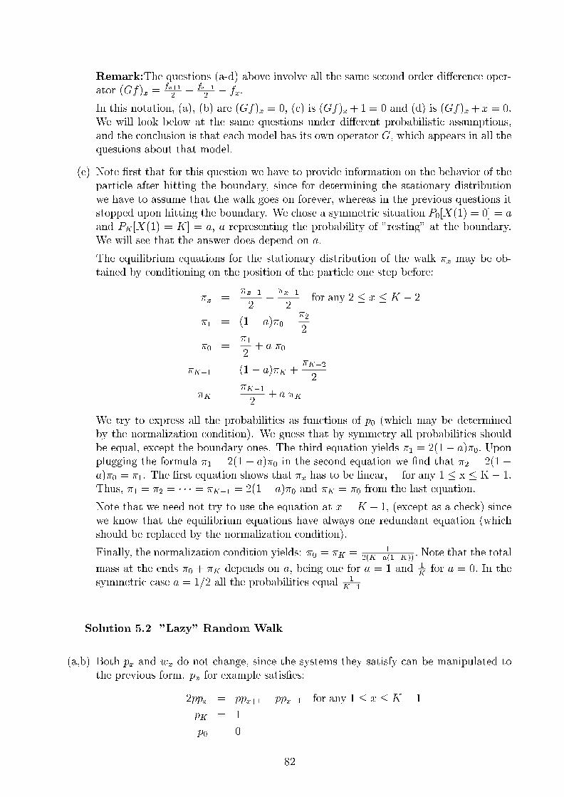
Remark:The questions (a-d) above involve all the same second order di�erence oper-
ator (Gf)x =fx+12
+ fx�12� fx.
In this notation, (a), (b) are (Gf)x = 0, (c) is (Gf)x+1 = 0 and (d) is (Gf)x+ x = 0:
We will look below at the same questions under di�erent probabilistic assumptions,
and the conclusion is that each model has its own operator G; which appears in all the
questions about that model.
(e) Note �rst that for this question we have to provide information on the behavior of the
particle after hitting the boundary, since for determining the stationary distribution
we have to assume that the walk goes on forever, whereas in the previous questions it
stopped upon hitting the boundary. We chose a symmetric situation P0[X(1) = 0] = a
and PK [X(1) = K] = a; a representing the probability of "resting" at the boundary.
We will see that the answer does depend on a:
The equilibrium equations for the stationary distribution of the walk �x may be ob-
tained by conditioning on the position of the particle one step before:
�x =�x+1
2+�x�12
for any 2 � x � K � 2
�1 = (1� a)�0 +�2
2
�0 =�1
2+ a �0
�K�1 = (1� a)�K +�K�22
�K =�K�12
+ a �K
We try to express all the probabilities as functions of p0 (which may be determined
by the normalization condition). We guess that by symmetry all probabilities should
be equal, except the boundary ones. The third equation yields �1 = 2(1� a)�0: Upon
plugging the formula �1 = 2(1� a)�0 in the second equation we �nd that �2 = 2(1�a)�0 = �1. The �rst equation shows that �x has to be linear, for any 1 � x � K� 1:
Thus, �1 = �2 = � � � = �K�1 = 2(1� a)�0 and �K = �0 from the last equation.
Note that we need not try to use the equation at x = K � 1; (except as a check) since
we know that the equilibrium equations have always one redundant equation (which
should be replaced by the normalization condition).
Finally, the normalization condition yields: �0 = �K = 12(K+a(1�K))
: Note that the total
mass at the ends �0 + �K depends on a; being one for a = 1 and 1Kfor a = 0: In the
symmetric case a = 1=2 all the probabilities equal 1K+1
Solution 5.2 "Lazy" Random Walk
(a,b) Both px and wx do not change, since the systems they satisfy can be manipulated to
the previous form. px for example satis�es:
2ppx = ppx+1 + ppx�1 for any 1 � x � K � 1
pK = 1
p0 = 0
82
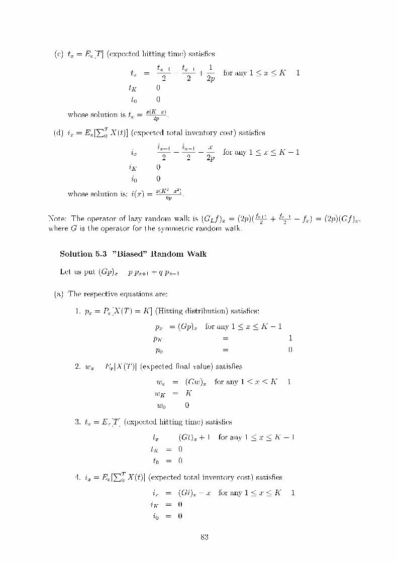
(c) tx = Ex[T ] (expected hitting time) satis�es
tx =tx+1
2+tx�12
+1
2pfor any 1 � x � K � 1
tK = 0
t0 = 0
whose solution is tx =x(K�x)
2p:
(d) ix = Ex[PT
0 X(t)] (expected total inventory cost) satis�es
ix =ix+1
2+ix�12
+x
2pfor any 1 � x � K � 1
iK = 0
i0 = 0
whose solution is: i(x) = x(K2�x2)6p
:
Note: The operator of lazy random walk is (GLf)x = (2p)(fx+12
+ fx�12� fx) = (2p)(Gf)x;
where G is the operator for the symmetric random walk.
Solution 5.3 "Biased" Random Walk
Let us put (Gp)x = p px+1 + q px�1
(a) The respective equations are:
1. px = Px[X(T ) = K] (Hitting distribution) satis�es:
px = (Gp)x for any 1 � x � K � 1
pK = 1
p0 = 0
2. wx = Ex[X(T )] (expected �nal value) satis�es
wx = (Gw)x for any 1 � x � K � 1
wK = K
w0 = 0
3. tx = Ex[T ] (expected hitting time) satis�es
tx = (Gt)x + 1 for any 1 � x � K � 1
tK = 0
t0 = 0
4. ix = Ex[PT
0 X(t)] (expected total inventory cost) satis�es
ix = (Gi)x + x for any 1 � x � K � 1
iK = 0
i0 = 0
83

(b) Let px;K denote the probability that the random walk starting at x will ever reach
a positive integer K and qx;K denote the probability of never reaching K (that is of
getting lost at �1). Now qx;x+1 (and hence px; x+ 1 also) is independent of x; since
the probability of never leaving a half line cannot depend on the label we put to its
right end. Letting r denote px;x+1, we see by the Markov property that px;K = rK�x:
Since p0;1 = p + qp�1;1 and thus r = p + q r2; we �nd that r may equal either pqor 1:
By the law of large numbers, the �rst case will occur if p < q and the second when
p > q. (To resolve the case p = q, more work is necessary; one way is to �nd p0;1 in
the presence of an extra lower barrier at L and then let L! �1:)
(c) We have to solve:
t(x) = p t(x+ 1) + q t(x� 1) + 1
t(�1) "does not blow up exponentially"
t(K) = 0
The roots of the auxiliary equation are qpand 1: The particular solution is �x
p�q and the
general solution of the nonhomogeneous recurrence is is t(x) = a(q=p)x + b+ �xp�q :
The �rst term blows up exponentially at �1 and so a = 0: Using the boundary
condition we get t(x) = K�xp�q : Thus t(0) =
Kp�q :
5.4 X(t) denotes simple random walk on the cube [0; 1]3, ~0 denotes the origin (0; 0; 0);
the opposite corner (1; 1; 1) is denoted by u: We note a symmetric role in all the questions
for all the neighbours of the origin, which allows us to denote them by the same letter
a = (0; 0; 1); :::: Similarly, we denote the neighbours of u by b = (0; 1; 1); ::::
a) To �nd tu = Eu[T0]; we solve the system:
tu = 1 + tb
tb = 1 +2
3ta +
1
3tu
ta = 1 +2
3tb
whose solution is ta = 7; tb = 9; tu = 10:
b) E0[ �T0] where �T0 is the expected time until revisiting 0 starting from 0; is given by
1 + ta = 1 + 7 = 8: Note that is precisely the inverse of the long run probability of being at
0; which is a well known result on expected return times.
c) Pa[X(T ) = u]; is obtained from the solution of
pa =2
3pb
pb =2
3pa +
1
3
which is pb =35; pa =
25:
84

d) Let pk be the probability of exactly k visits to (1; 1; 1) before returning to 0: Then p0is the same as the probability starting at a that the walk returns to 0 before visiting (1; 1; 1);
which is 35:
p1 = (25)2; p2 = (2
5)2(3
5); and in general pk = (2
5)2(3
5)k�1: (Check that
P1k=1 pk =
25; as it
should).
85

6 Di�erential equations for functionals of Brownianmotion
In some ways, Brownian motion is a very complicated process; it has very "wiggly" paths,
with quite unusual properties. For example, its path is nowhere di�erentiable, and after
reaching any level, its graph will cross that level an in�nite number of times in any neigh-
borhood, no matter how small, of the �rst crossing.
Despite these "path" complexities, problems of computing expectations or probabilities
may always be reduced to the relatively easy task of solving di�erential equations (ordinary
or partial). y
These di�erential equations maybe obtained by passing to the limit in the random walks
approximations for standard Brownian motion and Brownian motion with drift, which were
introduced in Sections 1.1.5, 1.1.6 respectively. z
De�nition: In�nitesimal random walk is a process time intervals of h:We found out
in Section 1.1.5 that symmetric random walk may converge to a �nite limit i� D2 = �2h;
for some �: This type of scaling needs to be enforced because it ensures that the variance of
the process Sh(t) converges to a �nite limit when h! 0:
(Note that VarSh(t) � thEZ2
1 = tD2
h:)
To approximate Brownian motion without drift �Bt ( where Bt is standard Brownian
motion which corresponds to the subcase � = 1:) we employ symmetric in�nitesimal
random walk with equal probabilities for going up(down), and to approximate Brownian
motion with drift �t+ �Bt we employ in�nitesimal random walk with vanishing bias
with probabilities for going up(down) of p; q = 12� �
2�2D (which converge both to 1
2when
D ! 0).
6.1 Ito's formula for Brownian motion
We will establish �rst Ito's formula for symmetric in�nitesimal random walk and then pass
to the limit.
To motivate the result, consider �rst the problem of determining the probability p(x) =
PxfTK � TLg of exiting through the upper barrier for symmetric in�nitesimal random walk.
yThe fact that we may practically bypass all the complexities of Brownian motion is quite reassuring, ifwe bear in mind that Brownian motion doesn't actually exist in real life. In practice, we always only observerandom walk and model it as Brownian motion or as Levy process with jumps; clearly, discussing whetherthe random walk we observe is indeed continuous (i.e Brownian motion) or rather whether it jumps duringthe periods of time when we can't observe it is rather an academic topic.
zIn fact, the property that computing expectations maybe reduced to solving various types of di�erentialproblems is shared by all stationary Markov processes, which may all be characterized by a di�erential,integral or di�erence operator G called generator. Our results in this section are purposely formulated interms of this operator, so that the result for other processes may be obtained simply by substituting thecorresponding generator.
86

Just as in the case D = h = 1; we see that p(x) must satisfy
p(x) = 1=2p(x+D) + 1=2p(x�D)
p(K) = 1
p(L) = 0
We could solve this as a di�erence equation just as in the case D = h = 1; but we want
to make here the point that things get slightly easier when D ! 0; due to the following
Exercise 6.1 Ito's lemma for in�nitesimal random walk
Show that for any function f(Sh(t) applied to a process Sh(t) which jumps right or left
by dx = D after time intervals of size dt = h; where D;h! 0 such that D2 = �2h we have:
a) 1=2f(x+D) + 1=2f(x�D)� f(x) � D2
2f 00(x) � hGf(x)
where Gf(x) = �2f 00(x)2
:
b) The expression approximated above is precisely the expected conditional di�erential
E [df(Sh(t)=Sh(t) = x] = E [(f(Sh(t+ h))� f(Sh(t))) =Sh(t) = x] of the function f(Sh(t))
over a small interval of size h; i.e:
E [df(Sh(t)=Sh(t) = x] = 1=2f(x+D) + 1=2f(x�D)� f(x)
c) E [d f(Sh(t)=Sh(t) = x] � hGf(x)
d) The expected new value of the function f(Sh(t)) after a small interval of size h is:
E [f(Sh(t+ h)=Sh(t) = x] = f(x) + hGf(x)
Solution 6.1 a) Using the Taylor expansions: f(x + D) � f(x) + f 0(x)D + f 00(x)2D2;
f(x�D) � f(x)� f 0(x)D + f 00(x)2D2; we �nd that for D small we have
f(x+D)
2+f(x�D)
2� f(x) � D2
2f 00(x)
Using the scaling, D2 = �2h we obtain �nally "Ito's lemma":
f(x+D)
2+f(x�D)
2� f(x) � hGf(x)
b) E [df(Sh(t)=Sh(t) = x] = E [(f(Sh(t+ h))� f(Sh(t))) =Sh(t) = x] = f(x+D)
2+ f(x�D)
2�
f(x)
c) Put a), b) together.
d) This follows from f(Sh(t+h)) = f(Sh(t))+f(Sh(t+h))�f(Sh(t)) = f(Sh(t))+df(Sh(t))
by taking expectations and using c):
87

E [f(Sh(t+ h))=Sh(t) = x] = E [f(Sh(t)) + df(Sh(t))=Sh(t) = x] � f(x) + hGf(x)
In the limit h! 0; symmetric in�nitesimal random walk converges to Brownian motion
with variability � and Exercise 1 yields:
Lemma 6.1. Ito's formula for Brownian motion with variability �
Let f(x) denote an arbitrary twice di�erentiable function applied to Brownian motionwith variability �; i.e. Xt = �Bt: Then, the expected value of the function after a small timeinterval may be approximated by:
E [f(Xt+h)=Xt = x] � f(x) + hGf(x)
where Gf(x) = �2
2f 00(x):
It is interesting to compare this result with the classical calculus "approximation" of the
di�erential of a function applied to a deterministic linear process Xt = �t: In that case we
have:
Lemma 6.2. First order Taylor approximation for df(Xt) when Xt is linear motionXt = x0 + �t
Let f(x) denote an arbitrary di�erentiable function applied to linear motion Xt = �t:Then, given that Xt = x; the value of the function after a small time interval may beapproximated by:
f(Xt+h) = f(x+ �h) � f(x) + h�f 0(x) = f(x) + hGf(x)
where Gf(x) = �f 0(x):
We take now a leap of faith to the case of Brownian motion with drift Xt = �t + �Bt;
which is composed from a linear drift �t and a Brownian motion with variability �: It turns
out that the generator is precisely the sum of the two individual generators
Lemma 6.3. Ito's formula for Brownian motion with drift
Let f(x) denote an arbitrary twice di�erentiable function applied to a Brownian motionwith drift Xt = �t+�Bt: Then, the expected value of the function after a small time intervalmay be approximated by:
E [f(Xt+h)=Xt = x] � f(x) + hGf(x)
where
(Gf)(x) =�2
2f 00(x) + �f 0(x) (33)
Proof sketch: The key point is again shoing that the di�erential of "in�nitesimal random
walk with vanishing drift" may be approximated by:
E [d f(Sh(t)=Sh(t) = x] = pf(x+D) + qf(x�D)� f(x) � f(x) + h(Gf)(x);
which is established in an Exercise below.
88

Note: Ito's formula may be also derived by a method which uses directly the properties of Brownian motion, to be covered
in a later section.
Summary: There are three approaches for working with Brownian motion with drift
Xt :
1. Xt = �t+ �Bt; which implies that EXt = �t;VarXt = �2t:
2. Xt � Sh(t) =Pbt=hc
1 Xi; where the "random walk with in�nesitemal bias" has incre-
ments Xi = �D which gpo up/down with probabilities p; q = 12� �
2�2D; and step size
satisfying D2 = �2h:
3. E f((Xt+h)=Xt = x] � f(x) + hGf(x) where (Gf)(x) = �2
2f 00(x) + �f 0(x):
The connection between one and two and two and three are established in the exercise 2a0
and 2b) below, respectively:
Exercise 6.2
a) Show that as the in�nitesimal random walk with vanishing bias and Brownian motion
with drift have the same expectation and variance, i.e. as h! 0; we have ESh(t)! �t and
VarSh(t)! �2t; respectively.
b) Show that for the in�nitesimal random walk with vanishing bias pf(x+D) + qf(x�D)� f(x) � h(Gf)x where (Gf)(x) = �2
2f 00(x) + �f 0(x):
Solution 6.2
b) Using the Taylor expansion, we �nd that for D small we have
pf(x+D) + qf(x�D)� f(x) =
p(f(x) +Df 0(x) +D2
2f 00(x) + :::) + q(f(x)�Df 0(x) +
D2
2f 00(x)� :::)� f(x) =
(p� q)Df 0(x) +D2f00(x)
2= h
��f 0(x) +
�2
2f 00(x)
�= h(Gf)(x)
where the last steps used the scaling relation D2 = �2 h and the relation (p� q) = ��2D:
Note: While the �rst derivative was enough by itself in standard deterministic calculus
to give a good approximation of the di�erential of a function, the addition of the uncertain
and "wiggly" Brownian motion leads to the necessity of using also the second derivative.
As illustrated in Exercise 2 below, the di�erential pf(x + D) + qf(x � D) � f(x) ap-
proximated by Ito's lemma appears in various problems involving functionals applied to
in�nitesimal random walk with vanishing bias. As a consequence, these problems maybe all
transformed by Ito's lemma into di�erential equations involving the di�erential operator
(Gf)(x) =�2
2f 00(x)
89
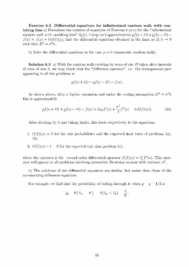
Exercise 6.3 Di�erential equations for in�nitesimal random walk with van-
ishing bias a) Formulate the systems of equations of Exercise 1 a)-c) for the "in�nitesimal
random walk with vanishing bias" Sh(t): Using Ito's approximation pf(x+D)+qf(x�D)�f(x) � f(x) + h(Gf)(x); �nd the di�erential equations obtained in the limit as D; h ! 0
such that D2 = �2h:
b) Solve the di�erential equations in the case � = 0 (symmetric random walk).
Solution 6.3 a) With the random walk evolving by steps of size D taken after intervals
of time of size h, we may check that the "di�erence operator", i.e. the homogeneous part
appearing in all the problems is
pf(x+D) + qf(x�D)� f(x):
As shown above, after a Taylor expansion and under the scaling assumption D2 � �2h
this is approximately
pf(x+D) + qf(x�D)� f(x) � h(�f 0(x) +�2
2f 00(x) = h(Gf)(x)): (34)
After dividing by h and taking limits, this leads respectively to the equations:
1. (Gf)(x) = 0 for the exit probabilities and the expected �nal value of problems 1a),
1b).
2. (Gf)(x) + 1 = 0 for the expected exit time problem 1c).
where the operator is the second order di�erential operator (Gf)(x) = �2
2f 00(x): This oper-
ator will appear in all problems involving symmetric Brownian motion with variance �2:
b) The solutions of the di�erential equations are similar, but easier than those of the
corresonding di�erence equations.
For example, we �nd that the probability of exiting through K when p = q = 1=2 is
px = PfXT = Kg = PfTK < T0g =x
K:
90
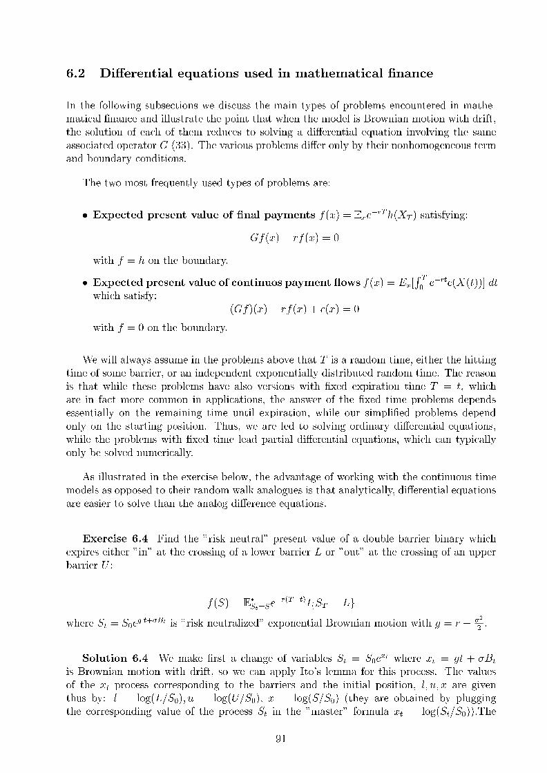
6.2 Di�erential equations used in mathematical �nance
In the following subsections we discuss the main types of problems encountered in mathe-
matical �nance and illustrate the point that when the model is Brownian motion with drift,
the solution of each of them reduces to solving a di�erential equation involving the same
associated operator G (33). The various problems di�er only by their nonhomogeneous term
and boundary conditions.
The two most frequently used types of problems are:
� Expected present value of �nal payments f(x) = E xe�rTh(XT ) satisfying:
Gf(x)� rf(x) = 0
with f = h on the boundary.
� Expected present value of continuos payment ows f(x) = Ex[R T0e�rtc(X(t))] dt
which satisfy:
(Gf)(x)� rf(x) + c(x) = 0
with f = 0 on the boundary.
We will always assume in the problems above that T is a random time, either the hitting
time of some barrier, or an independent exponentially distributed random time. The reason
is that while these problems have also versions with �xed expiration time T = t, which
are in fact more common in applications, the answer of the �xed time problems depends
essentially on the remaining time until expiration, while our simpli�ed problems depend
only on the starting position. Thus, we are led to solving ordinary di�erential equations,
while the problems with �xed time lead partial di�erential equations, which can typically
only be solved numerically.
As illustrated in the exercise below, the advantage of working with the continuous time
models as opposed to their random walk analogues is that analytically, di�erential equations
are easier to solve than the analog di�erence equations.
Exercise 6.4 Find the "risk neutral" present value of a double barrier binary which
expires either "in" at the crossing of a lower barrier L or "out" at the crossing of an upper
barrier U :
f(S) = E�St=S
e�r(T�t)IfST = Lgwhere St = S0e
g t+�Bt is "risk neutralized" exponential Brownian motion with g = r � �2
2:
Solution 6.4 We make �rst a change of variables St = S0ext where xt = gt + �Bt
is Brownian motion with drift, so we can apply Ito's lemma for this process. The values
of the xt process corresponding to the barriers and the initial position, l; u; x are given
thus by: l = log(L=S0); u = log(U=S0); x = log(S=S0) (they are obtained by plugging
the corresponding value of the process St in the "master" formula xt = log(St=S0)):The
91

functional becomes f(x) = E x0=xe�rT IfXT = log(L=S0)g where T = minfTl; Tug and are all
obtained from the change of scale S = S0ex; This is a discounted �nal payment problem,
and the �nal payo� is either 1 or 0 and so we must solve the associated di�erential equation:
�2
2f 00(x) + gf 0(x)� rf(x) = 0
f(l) = 1
f(u) = 0:
Letting a1; a2 enote the roots of the associated equation �2
2a2+ (r� �2
2)a� r = 0 we �nd
that a1 =�2r�2; a2 = 1 and
f(x) =ea1(x�u) � e(x�u)
ea1(l�u) � e(l�u)
In terms of the original variables this becomes
f(S) =(S=U)a1 � (S=U)
(L=U)a1 � (L=U)
6.2.1 Expected �nal payments
De�nition: An expected �nal payment functions is a function of the form:
f(x) = E xh(XT )
where h(x) denotes some �nal payment.
The time T could be taken as �xed, like in the problem of European options; however, this
leads to more complicated (partial) di�erential equations. For this reason we will consider
only the mathematically simpler case when T is a random time, like for example the hitting
time of a boundary.
The most typical example, discussed below, is that of escape probabilities, in which
the boundary is divided in a "good" part A where the payment is 1 and a "bad" part where
the payment is 0: The payment is thus h(x) = IA(x):
Lemma 6.4. The expected �nal payment problem leads to the equation
Gf(x) = 0
with f = h on the boundary.
Proof: We may either consider the approximating discrete problem pf(x+D) + qf(x�D)� f(x) = 0 and use its Taylor approximation pf(x+D) + qf(x�D)� f(x) = h(Gf)(x)
or work directly in continuous time conditioning on the value after a small time interval h
as follows:
f(x) = E xh(XT ) = E xEXhh(XT ) = E xf(Xh) = f(x) + h(Gf)(x)
92

where the last step follows from Ito's lemma. Cancelling f(x) and dividing by h yields
now the di�erential equation. The boundary conditions are obvious if we are already at the
boundary, the expected payment must equal the �nal payo�).
Example 1: Escape probability from an an interval [L;K]
We compute now fx = PxfX(T ) = Kg that a Brownian motion with drift X(t) starting
at x will exit an interval [L;K] through the upper endpoint.
We consider �rst the associated discrete biased random walk. The di�erence equation
satis�ed by the probability p(x)
px = PxfSh(T ) = Kgfor the associated discrete biased random walk are:
p(x) = p p(x+D) + q p(x�D)
p(K) = 1
p(0) = 0
Using Taylor expansions carefully, we �nd that p p(x+D)+q p(x�D)�p(x) � h (�2
2p00(x)+
�p0(x)) and so the system becomes
�2
2p00(x) + � p0(x) = 0
p(K) = 1
p(0) = 0
Note: As expected, this is of the form
(Gp)(x) = 0
p(K) = 1
p(0) = 0
where (Gp)(x) = �2
2p00(x) + � p0(x):
The general solution of the equation above is
p(x) = A1 (exp (�2�
�2x) + A2)
which after using the boundary conditions yields
p(x) =exp (�2�
�2x)� 1
exp (�2��2K)� 1
=f(x)� 1
f(K)� 1
where f(x) = exp (�2��2x):
93

6.2.2 Expected total continuous payments
De�nition: Expected continuous payment functions are functions of the form
f(x) = Ex[
Z T
0
c(X(t))] dt
where c(x) represent the rate of payment (cost) per unit time.
Note: This represents the continuous time limit of the discrete costsP[T=h]
i=0 c(X(i h))h when
h! 0:
We will work for convenience mostly with the case when T is a random time, for example
the hitting time of some boundary.
Lemma 6.5. An expected continuous payment function f(x) must satisfy:
(Gf)(x) + c(x) = 0
with f = 0 on the boundary.
We may either proof this by considering an approximating discrete problem and using
the Taylor approximation (??) or by working directly in continuous time, conditioning on
the value after a small time interval h:
Proof 1: For the random walk which approximates Brownian motion with drift we �nd
by conditioning after one step the inhomogeneous equation:
f(x) = p f(x+D) + q f(x�D) + h c(x)
which after using the Taylor approximation (??) reduces to:
h (�2
2f 00(x) + � f 0(x)) + c(x)) = 0:
yielding in the limit: (Gf)(x) + c(x) = 0 where Gf denotes the Brownian motion with drift
operator �2
2f 00(x) + � f 0(x):
Proof 2: Working directly in continuous time, we condition on the value after a small
time interval h:
f(x) = E x
Z T
0
c(Xt)dt =
E x
Z h
0
c(Xt)dt+ E x
Z T
h
c(Xt)dt � c(x)h+ E xEXh
Z T
h
c(Xt)dt =
c(x)h+ E xf(Xh) � c(x)h+ f(x) + hGf(x)
94

where the last step used Ito's lemma.
Cancelling f(x) and dividing by h yields now the di�erential equation. The boundary
conditions are obvious (the total cost over a 0 length interval is 0).
scr Note: The second proof rests only on the Ito's lemma previously obtained for Brow-
nian motion with drift. Ito's lemma is also true for a more general class of processes called
di�usions (These processes, discussed in the next section, are basically Brownian motions
for which the drift �(x) and volatility �(x) are allowed to depend on the current position).
Hence, the lemma above also holds in that more general framework.
One example is when c(x) = 1 identically, in which case f(x) becomes the expected exit
time t(x) = E xT:
Example 2: The expected exit time from (L;K) for a Brownian motion with
drift
We have found in Exercise 2 that the expected time t(x) when starting at x until exiting
(L;K) for Brownian motion without drift is the solution of
(Gt)(x) + 1 = 0
t(K) = 0
t(L) = 0
where (Gt)(x) = �2
2t00(x) is the generator of Brownian motion without drift. It is easy to
guess (and check) that the procedure of considering the biased random walk approximation
and passing to the limit will yield the di�erential equation:
(Gt)(x) + 1 = 0
t(K) = 0
t(L) = 0
where (Gt)(x) = �2
2t00(x)+� t0(x) is now the generator of Brownian motion with drift. Thus,
we must solve:
�2
2t00(x) + � t0(x) + 1 = 0
t(K) = 0
t(L) = 0
Solution: The homogeneous solution p(x) = A1 (exp (�2��2x) + A2) was obtained in the
previous problem.
Our initial guess for a particular solution is tp(x) = B; but we have to modify it to
tp(x) = Bx, since constants satisfy the homogeneous problem. We �nd that B = � 1�and
tp(x) = �x�:
95

The general solution is thus of the form t(x) = �x�+ a (exp (�2�
�2x) + b): The boundary
conditions yield
t(x) = �x� L
�+K
�
exp (�2��2x)� exp (�2�
�2L)
exp (�2��2K)� exp (�2�
�2L)
= tp(x)� tp(K)f(x)� f(L)
f(K)� f(L)
where tp denotes the particular solution which is 0 at x = L and f(x) = exp (�2��2x) is the
nonconstant homogeneous solution.
Example 3: The expected total inventory cost problem over T = min(T0; TK)
until exiting (0;K) for Brownian motion with drift. The cost
i(x) = E x
Z T
0
Xtdt
must satisfy:
(Gi)(x) + x = 0
i(K) = 0
i(0) = 0
Plugging the generator of Brownian motion with drift leads to:
�2
2i00(x) + � i0(x) + x = 0
i(K) = 0
i(0) = 0
The particular solution (obtained by modifying once the initial trial Ax+B is of the form
ip(x) = Ax2+Bx: By the method of undetermined coeÆcients we �nd that ip(x) =x2
�2�+x�2
2�2:
Finally, as in Example 1, we �nd from the boundary conditions that:
i(x) = ip(x)� ip(K)f(x)� f(0)
f(K)� f(0)
where f(x) = exp (�2��2x) is the nonconstant homogeneous solution and ip denotes the par-
ticular solution which is 0 at x = 0.
96

6.2.3 Expected discounted �nal payments
De�nition: Expected discounted �nal payment functions are functions f(x) of the form:
f(x) = E xe�rTh(XT )
Lemma 6.6. Expected discounted �nal payment functions satisfy:
Gf(x)� rf(x) = 0
with f = h on the boundary.
Proof:
f(x) = E xe�rTh(XT ) = e�rhE xe
�r(T�h)h(XT )
= e�rhE xEXhe�r(T�h)h(XT ) � (1� rh)E xf(Xh)
� (1� r h) (f(x) + hGf(x)) � f(x) + h((Gf(x)� r f(x))
where the last steps consist in using Ito's lemma and ignoring the h2 term.
A typical example is the present value of a double barrier option which "kicks in" if a
lower barrier L is reached and expires if an upper barrier U is reached.
6.2.4 Expected present value of continuous payment ows
De�nition: Expected present value of continuous payment functions are functions of the
form
f(x) = Ex[
Z T
0
e�rtc(X(t))] dt
where c(x) represent the rate of payment (cost) per unit time.
Lemma 6.7. An expected continuous payment function f(x) must satisfy:
(Gf)(x)� rf(x) + c(x) = 0
with f = 0 on the boundary.
A typical example is the present value of a �xed dividend k, to be payed until the asset
hits an upper barrier u:
6.3 Summary
Two general types of functionals are most common in problems of valuation of barrier options
exercised at some stopping time T : expected �nal payo�s and expected continuous payments.
Each has also a version with discounting and they may be all incorporated as particular
cases in a general formula called the Feynman-Kac formula. Each problem leads to a certain
associated ordinary di�erential equation:
97

� Expectation of �nal payo�s f(x) = E xh(XT ) satisfying:
Gf(x) = 0
with f = h on the boundary.
� Expected total continuous payments f(x) = E x
R Tt=1
c(Xt)dt satisfying:
(Gf)(x) + c(x) = 0
with f = 0 on the boundary.
� Expected discounted �nal payo�s f(x) = E xe�rTh(XT ) satisfying:
Gf(x)� rf(x) = 0
with f = h on the boundary.
� Expected present value of continuous payment ows f(x) = Ex[R T0e�rtc(X(t))] dt
which satisfy:
(Gf)(x)� rf(x) + c(x) = 0
with f = 0 on the boundary.
� The Feynman-Kac formula
f(x) = Ex[e�R T0r(Xu)duh(XT ) +
R T0e�
R t0r(Xu)duc(X(t))] dt satis�es:
(Gf)(x)� r(x)f(x) + c(x) = 0
with f = h on the boundary.
Note that the general Feynman-Kac formula allows a non constant random discount rate
r(Xu); which is more realistic; for this to be really useful in applications however, Xt has to be
interpreted as some vector composed of several indices which determine (deterministically)
the interest rate. Thus, Xt is not to be interpreted as a single asset anymore, but as some
"multifactor" which drives the economy.
Each of these problems has also a version with �xed expiration time, which involves
however an extra variable (the remaining time until expiration) and lead to solving partial
di�erential equations. For example, the present value of �nal �xed time payment
functional:
f(x; t) = E x;te�rth(Xt)
which satis�es@
@tf + (Gf)� rf = 0
with f(x; t) = h(x) at the �nal time.
The last and (more commonly used in practice) example is di�erent of the previous four
in that the expectation depends on two variables: the starting point x and the current time
98

t (or rather on the remaining time T � t. This leads to partial di�erential equations,
which look similar to the ordinary di�erential equations previously discussed, but are actually
considerably harder to solve.
This partial di�erential equation could be derived in principle by the usual method of starting with a discrete approximation,conditioning on one step and taking limits, or by starting with the partial di�erential equation satis�ed by the density of standardBrownian motion:
** Extra problem a) Show that the normal density p(t; x) =exp (� x2
2�2 t)
p2��2 t
satis�es the partial di�erential equation
@
@tp+
@2
@x2p = 0
b) Conclude that g(x; t) = Ex;th(XT ) =Rp(t; x� y)h(y)dy satis�es the same partial di�erential equation.
c) Derive the partial di�erential equation satis�ed by f(x; t) = e�rtg(x; t):
While we need to be aware of the existence of these various PDE's (partial di�erential equations) for the expected present
values of options, because of their crucial role in solving the problems of mathematical �nance numerically via the use of
computers, we will not use them, since numerical approaches are not featured in this course.
99

6.4 Exercises
Exercise 6.5 IfB(t) is standard Brownian motion on the interval [L;K], �nd the probability
of exiting through the lower barrier px = PfTL � TKg:
Exercise 6.6 If B(t) is standard Brownian motion, �nd P0fT1 < T�1 < T2g.
Exercise 6.7 Prove Lemma 6.6, starting from the di�erence equation for the analog
problem for random walk with vanishing bias and taking the limit as D;h!1:
Exercise 6.8 Formulate and solve a di�erential equation for the expected exit time
from (L;1) for a Brownian motion with drift � < 0: Compare the result with the result
obtained in the deterministic case Xt = �t:
Exercise 6.9 "Bankruptcy time" Suppose that the evolution of an asset follows the
lognormal model St = exponential Brownian motionwith a negative parameter g: The asset
will be liquidated at the stopping time Ta = infft : St = ag when its value reduces to e�a;where a is a number less than 1: Find the expected value of the time Ta:
Exercise 6.10 Find the "risk neutral" present value of a perpetual (no time limit)
"down and in" lower barrier binary:
f(S) = E�Se
�rTLIfTL <1gwhere St = S0e
g t+�Bt is "risk neutralized" exponential Brownian motion with g = r � �2
2:
Exercise 6.11 Perpetual American put: a) The perpetual barrier put: Find the
"risk neutral" present value of a "perpetual" put-barrier option with �nal payment (K �ST )+ = K �L; to be exercised the �rst time when the stock price crosses a lower barrier L:
b) Suppose the buyer of the option can choose the barrier L at which to exercise (this is
called an American option). What is the optimal choice for the barrier?
Exercise 6.12 Find the present value of a �xed dividend k, to be payed until the asset
hits an upper barrier u:
f(x) = E x
Z T
0
e�rtkdt
where Xt = S0eg t+�Bt is exponential Bronian motion and T = Tu is the hitting time of the
barrier.
Exercise 6.13 a) Formulate and solve a di�erential equation for the expected total
inventory cost until hitting 0 for a deterministic case Xt = �t with � < 0:
100

b) Formulate and solve a di�erential equation for the expected total inventory cost until
hitting 0 for a Brownian motion with drift � < 0: Compare the result with the result obtained
in the deterministic case Xt = �t:
101

6.5 Solutions
Solution 6.5 We need a formula for PxfTL < TKg for a general state space [L;K]: This is
a generalization of the previous "probability of hitting K before 0 problem. The di�erential
equation is
Gf = 0
f(L) = 1
f(K) = 0
where (Gf)(x) = 12f 00(x)
and the solution is K�xK�L :
Solution 6.6 By the general rule for conditional probabilities, P0fT1 < T�1 < T2g =
P0fT1 < T�1gP1fT�1 < T2= conditional on fT1 < T�1gg: We can however ignore the con-
ditioning since B(t) is a Markov process. Furthemore, by the stationarity of increments,
P1fT�1 < T2g = P0fT�2 < T1g.
Applying the result of the previous exercise twice, we �nd
P0fT1 < T�1 < T2g =1
2
1
3=
1
6:
Solution 6.7 The expected present value f(x) = E xe�r�h(X� ) satis�es:
f(x) = e�rh(pf(x+D) + qf(x�D)
The boundary conditions are f(K) = h(K); f(L) = h(L):
After a Taylor expansion, using the scaling relation D2 = �2h and the fact that p; q =12� �
2�2D satisfy p� q = �
�2D; we �nd:
f(x) � (1� rh)
�p(f(x) +Df 0(x) +
D2
2f 00(x) + :::) + q(f(x)�Df 0(x) +
D2
2f 00(x)� :::)
�
� f(x) + h
��f 0(x) +
�2
2f 00(x)
�= h(Gf)(x)
Solution 6.8
�2
2t00(x) + � t0(x) + 1 = 0
t(1) is not "exponentially blowing up"
t(L) = 0
102

Solving this, or passing to the limit K !1 in the result of Example 2 (using � < 0) we
�nd t(x) = �x�L�:
Interestingly, this does not depend on the volatility parameter � and is in fact the same
answer we obtain in the deterministic case � = 0; i.e. when Xt = �t:
Solution 6.9 The Expected Bankruptcy time
Solution 6.10 "Down and In" binary: We make �rst a change of variables St = S0ext
where xt = gt + �Bt is Brownian motion with drift, so we can apply Ito's lemma for this
process. The functional becomes f(x) = EX0=xe�rT IfTl < 1g where l = log(L=S0) and
x = log(S=S0): This is a discounted �nal payment problem, and so we must solve the
associated di�erential equation:
�2
2f 00(x) + gf 0(x)� rf(x) = 0
f(l) = 1
f(1) = 0:
This homogeneous equation has two exponential solutions ea1x; ea2x where a1; a2 are the
roots of the equation �2
2a2 + (r � �2
2)a� r = (�
2
2a+ r)(a� 1) = 0: The solution ex blows up
at 1 so it can't be used. In conclusion, f(x) = e�2r
�2(x�l): Back to the original variables we
�nd
f(S) = (L=S)2r
�2
Note: an alternative derivation is via the Wald martingale; note that a2 = � 2r�2is precisely
the negative root of Wald's equation c(a) = r:
Solution 6.11 Perpetual American put: a) The value of the perpetual put barrier
is the value of a "down and in" binary (see the previous Exercise) multiplied by K � L:
f(S) = (K � L)(L=S)2r
�2
b) The optimal exercise barrier is found by setting the derivative with respect to L equal to
0: ....
We note that it does not depend on the initial starting point S (this is due to the Markov
property of the asset model).
Solution 6.12 Dividend until an upper barrier:
Solution 6.13
a) The deterministic discrete approximating equation is f(x) = hc(x)+f(x+� h) di�ers
103

from the random walk one by containing only one possible for X at time t+ h, which in the
limit results in a �rst order equation, as opposed to second order in the random case.
� f 0(x) + c(x) = 0
f(0) = 0
If, say, c(x) = x; the solution is x2
�2� ; as can be easily checked directly (the emptying timeis x
�� and the cost is the area of a triangle with sides x; x�� .
It is interesting to compare the stochastic inventory problem with the deterministic case
(corresponding to � = 0) when X(t) = x + �t: For large x; the dominant �rst term in the
solution above is independent of the uncertainty parameter � and coincides in fact with the
integral of the deterministic emptying solution x+ �t: For small x however � is important.
104

7 Financial variations on Black Scholes
In this section we review the Black Scholes theory and discuss some extensions.
We start by recalling the valuation formula for the forward on an asset
F = S0
and the valuation formula for the call option, which, taking into account the previous
identity, will be written this time as:
C = F�
log( F
~KT)
pVT
+
pVT
2
!� ~KT�
log( F
~KT)
pVT
�pVT
2
!
The point of this new formulation is that it turns out to be also true in other aplications
discussed below, in which the forward value isn't equal anymore to the current asset value.
More speci�cally, this formula continues to apply in the case of assets on a foreign exchange,
with the forward price of a foreign stock being given by
F = S0E0
where E0 denotes the initial exchange rate, and in the case of options on foreign currencies
with interest rate y and current exchange rate E0 or on assets yielding continuous dividends
at rate Æ; in which case the forward prices are:
F = E0e�yT and F = S0e
�ÆT
7.1 Assets on a foreign exchange
A british investor invests in a stock on the Japanese exchange. It is assumed that the stock's
value evolves as geometric Brownian motion St = eXt ; where Xt = g1t+�1B1(t) is Brownian
motion with drift g1 and variance �21: Suppose that the interest rates in Britain is r, and
that the exchange rate is such that 1 yen will be worth at time t Et = E0eg2t+�2B2(t) where
B1(t); B2(t) are Brownian motions with correlation �t:
To �gure out the risk neutral sterling value of various �nancial derivatives it is enough to
note that the sterling value of a foreign asset StEt is itself an exponential Brownian motion
given by StEt = egt+�Bt where g = g1 + g2 and �2 = �21 + �22 + 2��1�2 (the latter follows
from the addition formula for correlated Gaussian random variables). In conclusion, the
usual formulas for call, put, etc. apply, where however S0 is replaced by S0E0; the latter is
precisely the forward value of ST for the British investor.
A somewhat unusual barrier option is described in the following exercise:
105

Exercise 7.1 Exchange adjusted barrier option
1. Let a > 0 and let Ta = infft : Xt = ag where Xt is standard Brownian motion.
Formulate and solve a di�erential equation for the Laplace transform of Tl
f(x) = EX0=x[e�rTl ]:
Conclude that the Laplace transform of Tl starting from X0 = 0 is:
E 0 [e�rTl ] = e�l
p2r; r > 0:
2. Using the previous answer (or otherwise) �nd the expectation E 0Tl:
What is the Laplace transform E 0 [e�rTl ] when r < 0? .
A british investor buys one unit of stock on the Japanese exchange, whose foreign
currency price evolves as geometric Brownian motion St = S0eXt; whereXt is standard
Brownian motion with X0 = 0. Suppose that the interest rates in both countries are
0, and that the exchange rate is such that 1 yen will be worth at time t Et = E0e��t+�Bt
where Bt is a Brownian motion independent of Xt and � > 0 (a strong pound).
The investor decides to sell the stock at the time T when the foreign currency price
S0eXt reaches a pre-determined level S0e
l > S0 (so l > 0). The exercise illustrates the
fact that the pro�ts of this strategy, which disregards the real value StEt of the asset
for the british investor, will be usually eroded by the strong pound.
3. What is the value of the investment at time t in the investor's currency (in pounds).
Find an expression for the expected �nal payo� per pound invested.
4. Conditioning on the value of T; �nd the expected �nal value of the (exchange adjusted)
investment if the parameters � and � satisfy 2� > �2, and determine under what
conditions the pro�t is negative and positive, respectively.
5. Explain what happens if 2� < �2 and comment.
Solution 7.1
1. This problem is already expressed in terms of a standard Brownian motion Xt: It may
be viewed as computing the expected discounted value of a sure payo� of 1 achieved
when the boundary l is hit by Xt: The di�erential equation is:
1
2f 00(x)� rf(x) = 0
f(l) = 1
f(�1) = 0
with solution f(r; x) = e(x�l)p2r: Note this only works when r > 0:
For x = 0 we �nd f(r; 0) = e�lp2r
106

2. Di�erentiating the Laplace transform f(r; 0) of Ta with respect to r and plugging r = 0
we �nd E 0Tl = � @@rf =1:
When r < 0 we expect E[e�rTl ] =1 since Tl and so �rTl is likely to be very large, orsince the discounting is negative and so the value keeps increasing, for a time which
has in�nite expectation.
More formally, using ex > 1 + x we see that for any l and r < 0 we have E[e�rTl ] >1 + (�rE 0Tl) =1:
3. The (exchange adjusted) value of the investment in the investor's currency is given by:
E0e��t+�BteXt: The expected �nal payo� per pound invested is E [ele��T+�BT ]; (where
we put T = Tl).
4. Let fT (t)dt denote the stopping time's density. Conditioning on T = t we �nd:
E [ele��T+�BT ] = elZt
fT (t) dt e��t
E [e�BT =T = t]
= elZt
fT (t) dt e��te
�2t2 since T is independent of Bt
= elZt
fT (t) dt e�(���2
2)t = elE e�rTa
where we put r = � � �2
2: If r > 0 (which happens if 2� > �2) we may conclude by
part a) that the expected �nal value is
ele�lp2� = el(1�
p2�
The pro�t has negative expectation i� the expected �nal payo� per pound will be
smaller than 1: This happens i� the exponent of l 1 �p2r is negative, i.e. i� 2r =
2� � �2 > 1; or 2� > �2 + 1: In this case the strong pound is expected to erode the
investor's pro�ts!
The pro�t has positive expectation i� the exponent is positive, i.e. i� �2 < 2� < �2+1:
5. If 0 < 2� < �2 then we have in�nite expected pro�ts by (b).
7.2 Options on currency and on assets yielding dividends
Consider �rst the case of a forward on a unit of foreign currency, say yens, which evolve
as Yt = Y0eyt: Assume the exchange value is given by exponential Brownian motionEt =
E0e�t+�Bt of home currency units for each yen (and the home currency brings interest r;
which will not be needed here).
It turns out just as in the case of forwards on assets that the best hedging strategy is
static, namely to buy foreign currency and hold it until expiration. However, since the
foreign currency produces interest, to have one unit later it is enough to buy e�yT units now,
which will require E0e�yT units of the home currency.
107

In conclusion, the forward value of a unit of foreign currency is
F = E0e�yT
Note the extra discount factor which decreases the current value with respect to the case
y = 0:
Precisely the same formulas holds in the case of assets which yield continuous dividends
at some rate Æ: Let St denote the value of one stock unit at time t and let Nt = N0eÆt
denote the number of stock units at time t for an investor who starts with N0 stock units
(this changes by exponential increase, just as in the case of cash producing �xed interest).
The total value of an investment evolves thus as ~St = NtSt = N0SteÆt; which is of the same
nature as the total value of a foriegn currency with constant interest. By the same argument
of static hedging, this leads to the same valuation for the forward, with the dividend rate Æ
replacing the interest rate y:
Furthemore, it turns out (we will not prove that) that the value of a call option is still
given by
C = F�
log( F
~KT)
pVT
+
pVT
2
!� ~KT�
log( F
~KT)
pVT
�pVT
2
!
In the next section we consider a more general �nancial derivative which involves an
exchange between two arbitrary assets.
7.3 Exchange options
De�nition Given any two assets S1; S2 an exchange option is de�ned as the right (but
not the obligation) to exchange asset S2 for asset S1; or of obtaining the payo� (S1 � S2)+:
Theorem 7.1. The value of an exchange option on two assets described by geometric Brow-nian motions:
Si(t) = Si(0)egi t+�iBi(t); i = 1; 2
where Bi(t) are Brownian motions with correlation � is given by:
E = F1�
log(F1~F2
)pVT
+
pVT
2
!� F2�
log(F1
F2)p
VT�pVT
2
!
where the remaining volatility is VT = T (�21 + �22 � 2��1�2):
To understand this formula, it is further useful to de�ne the "moneyness" of an exchange
bym1;2 =log(
F1F2
)pVT
: The moneyness is positive or negative depending on whether then exchange
is currently desirable or not. In terms of the moneyness, the value of the exchange option is
given by E = F1�(m1;2 +pVT2)� F2�(m1;2 �
pVT2) which may be summarized as:
The option seller should hedge by determining the moneyness of the exchange,
and keep positive (negative) proportions of the forward values of the �rst (sec-
ond) asset, computed by applying the normal cdf to the moneyness adjusted
upward(downward) by a factor proportional to the remaining volatility.
108

Note: 1) Two examples of exchange options are the call and the put. In the call case,
the moneyness is determined by taking the quotient of the present values (or current forward
values) F and ~KT of the stock unit and of the exercise price. In the put case, the reciprocal
quotient is used.
2) When K = 1; the forward value of one cash unit is also called a zero coupon bond.
The proof of the theorem above is left as an exercise.
Exercise 7.2 Derive the formula for the risk neutral value E e�rT (S1(T ) � S2(T ))+ of
an exchange option on two exponential Brownian motion assets
Si(t) = Si(0)egi t+�iBi(t); i = 1; 2
where B1; B2 are two Brownian motions with correlation �:
Hint: Use the price of the second asset as an arti�cial currency (called "numeraire").
The "numeraire" price of any asset S(t) is given by S(t)
S2(t); thus, the "numeraire" price of
the second asset is equal to 1 at any time t and in conclusion using "numeraire" puts us
in the situation when the second asset is constant. This is however precisely the previously
discussed case of a call option in a market with 0 interest rate, for which we may apply the
classical Black Scholes formula.
1. The "numeraire" price of the �rst asset becomes Yt =S1(t)
S2(t)What is the distribution of
Yt?
2. Find the "numeraire" Black Scholes value for exchanging Y (T ) by 1; as well as the
value of the exchange option E e�rT (S1(T )� S2(T ))+ measured in original currency.
3. Find the price of the standard call and put options on a GBM asset in a market with
interest rate r and show that they satisfy the "call-put" parity formula
C = P + F � ~K
Solution 7.2
1. Yt is also a geometric Brownian motion
Yt = egt+�Bt
with parameters g = g1 � g2 and with variance �2 = �21 + �22 � 2��1�2:
2. The "fair numeraire price" of the exchange option is obtained by plugging Y0 =S10S20
instead of S0 and 1 instead of K in the r = 0 Black Scholes formula (by risk neutrality,
this means assuming that Yt = e��2
2t+�Bt) yielding:
S1(0)
S2(0)�(
S1(0)
S2(0)+�2T
2p�2T
)� �(S1(0)
S2(0)��2T
2p�2T
).
109

The "fair original currency price" at time t is obtained by multiplying with S2(t). Thus,
for the initial value we have to multiply with S2(0); yielding S1(0)�(s)�S2(0)�(l) wheres; l =
S1(0)
S2(0)��2T
2p�2T
are the adjusted moneynesses. Replacing Si(0) by the forward values
Fi yields the �nal answer.
3. In the case of the call (put) options in markets with non zero interest rate, the cash
asset evolves as S2(t) = S20e
rt (S1(t) = S10e
rt) and its prescribed �nal value is K: The
forward (present) value is thus S2(0) = Ke�rT (S1(0) = Ke�rT ). We get the respective
formulas
C = S0�(s)�Ke�rT�(l) P = Ke�rT�(�l)� S0�(�s)
Since �(�x) = 1� �(x) we get the "put-call" parity relation:
P = Ke�rT � S0 + C = C + ~K � F
which has the clear investment interpretation that buying the stock and a put and
taking a loan of ~K is the same as buying a call.
7.4 Exercises
Exercise 7.3
a) Let l > x and let Tl = infft : Xt = lg. Formulate and solve a di�erential equation
for the Laplace transform f(x) = EX0=xe�rTl; if Xt is Brownian motion with drift �t and
variance �2t:
b) Using the previous answer (or otherwise) �nd the expectation E 0Tl:
c) Solve the analogous problem when x > l:
110

8 Canadian options
There is something missing currently from our picture on how to solve option problems by
di�erential equations, and the hole will be �lled by introducing a new type of options.
De�nition: A Canadian option is an option which expires after an exponentially
distributed random time �; independent of the asset process.
We have introduced thus three type of options, according to whether the expiration is:
1. At a �xed expiration time t; at which a �nal payo� hf (Xt) is earned; these are called
European options.
2. At the �rst time Tl when the process Xt crosses some barrier l; at which time a rebate
hb(XTl) is received; these will be called pure Barrier options.
3. At an exponentially distributed random time �; independent of the asset process; these
will be called Canadian options.
While alive, each type of option may also earn a continuous "interest" c(Xt):
scr Review of Section 3: We have learned how to valuate pure Barrier options via
di�erential equations. Provided we assume as usual an exponential Brownian motion model
St = S0eXt where Xt is Brownian motion with drift and provided we express the payments
hb(x); c(x) in terms of the variable Xt = log(St=S0); their value depends only on the initial
starting point x
v(x) = E�xe
�r thb(XTl) +
Z Tl
0
e�rtc(Xs)ds
satis�es the di�erential equation:
�2
2v00(x) + �v0(x)� rv(x) + c(x) = 0 (35)
v(l) = hb(l) (36)
where � = r � �2
2(to ensure risk neutrality of the valuation measure). Thus, the boundary
payment and the continuous "interest" enter the di�erential equation as boundary conditions
and nonhomogeneous terms, respectively.
We have not discussed yet the di�erential equation approach for the �rst and most com-
mon options, the European options, which were valued by a di�erent approach, making use
of the explicit formula available for the density of exponential Brownian motion assets at
any �nite time. The reason is that the value of European options with �nite time expiration
depend not only on the initial starting point x, but also on the remaining time until expi-
ration t: As such, they satisfy not ordinary, but partial di�erential equations (PDE's).
The purpose of this section is to show how Canadian options, whose value is also given by
ordinary di�erential equations, may be used to approximate the more complicated European
options.
Even in the simplest case of no barrier payo� and no interest
v(t; x) = E�xe
�r thf (Xt)
111
we are lead already to the PDE
Gv � rv � @
@tv = 0 (37)
v(0; x) = hf (x) (38)
where Gv(x) = �2
2v00(x) + (r � �2
2)v0(x)
In the general case of European options which have also a barrier payo� and continuous
interest, we are lead to:
Gv � rv + c(x)� @
@tv = 0 (39)
v(0; x) = hf (x) (40)
v(t; l) = hb(l) (41)
These PDE's may be derived by the usual method of conditioning on one step and
employing the random walk approximation, but we skip the derivations. Solving partial
di�ential equations is very rarely possible analytically; they are typically solved numerically
using computers, which are not featured in our notes.
However, the Canadian options last introduced can provide quite good approximations
for the value of European options. The idea is to approximate a European option with
remaining lifetime t via a Canadian option whose exponential lifetime � has the rate �
chosen by � = 1t; so that its expected duration is precisely E � = t:
We will show next that the value of Canadian options is independent of time and may be
obtained by solving ordinary di�erential equations, instead of partial ones. Probabilistically,
the independence of time is a consequence of the memoryless property of the exponential
lifetime. Analytically, it will be seen from the close relation between Canadian options and
Laplace transforms, discussed in the next section.
Notes: 1) Perpetual options are a particular case of Canadian options when � = 0:
2) The independence of time makes Canadian options simpler to price than European
options (just like perpetuals and pure barrier options). However, Canadian options are not
traded, and are not likely to ever be. Their practical implementation would require that the
seller maintains some type of "exponential clepsydra" and that the buyer trusts the seller
for letting him know when the option expired).
8.1 The Connection with Laplace transforms
Let v(t; x) = E�e�r thf (Xt) denote the value of an European option with �xed expiration t
and some �nal payo� hf (x): Then,
112

Lemma 8.1. The randomized or "Canadian" value of the option, de�ned as v�(�; x) =E�xe
�r�hf (X� ) where � is exponential with rate � is given by:
v�(�; x) =
Z 1
t=0
�e��tv(t; x)dt
where � = 1=t:
Proof: Conditioning on � = t we �nd:
v�(�; x) = E�x
Z 1
t=0
�e��tdt�e�rthf (Xt)
�=
Z 1
t=0
�e��tdt�E�xe
�rthf (Xt)�=
Z 1
t=0
�e��tv(t; x)dt
Note: By the lemma above, we see that the Canadian value di�ers from the Laplace
transform of the European value only by the extra factor �: This "almost" Laplace trans-
form, in which we average with respect to the exponential density, is called Laplace-Carson
transform.
One of the most important feature of Laplace transforms f̂(�) =R1t=0
e��tf(t)dt is thatthey transform derivative operations in multiplications, via the well known:
Lemma 8.2. The Laplace transform of a derivative is given by:
f̂ 0 = �f̂ � f(0)
By this property, taking Laplace transforms of di�erential equations changes them into
algebraic equations. The Laplace-Carson transform f�(�) =R i0e��tf(t)dt has of course the
same properties as the Laplace transform (plus the extra convenience of transforming con-
stants into constants), which is why considering Canadian values will rid us of the undesired
partial with respect to time.
The formula for transforming derivatives becomes:
Lemma 8.3. The Laplace-Carson transform of a derivative is given by:
(f 0)�(�) = �(f� � f0):
Applying now a Laplace-Carson transform in time, the partial di�erential equation (38)
turns into an ordinary di�erential equation.
Lemma 8.4. The Canadian value of a derivative with �nal payo� hf
v�(�; x) = E�xe
�r�hf (X� )
satis�es the ordinary di�erential equation:
Gv� � rv� � �(v� � hf ) = Gv� � (r + �)v� + �hf = 0
113

The proof of this lemma is left as an exercise.
Note: The di�erential equation above is precisely the same as that obtained for a perpetual option yielding continuousdividend �hf (Xs), if the interest rate was r + �: Thus,
v� = Ex
Z 1
0
e�(r+�)s�hf (Xs)ds
Example 1: Discontinuous payo�s Find the value of the Canadian digital
v(S) = E Se�r�IS��K
Solution: Converting to the variables Xt = log(St=S0) we �nd the converted �nal
payo�
IS��K = IS0eXt�K = IX��k
where k = log(K=S0): By lemma 5.4, v(x) must satisfy :
�2
2v00(x) + (r � �2
2)v0(x)� (r + �)v + �Ix�k = 0
v(�1) not exponentially increasing
One way to solve the di�erential equation above is by taking one more Laplace trans-
form, which will change all the derivatives into multiplication operations. However, a direct
approach is also possible.
Because the payo� is given by di�erent formulas below and above k; we must solve
each part separately. Let �1; �2 denote respectively the positive and negative roots of the
characteristic equation �2
2�2 + (r � �2
2)� � (r + �) of the homogeneous operator.
Below k we �nd v(x) = A1e�1(x�k) and above k we �nd �
r+�+A2e
�2(x�k): To complete thesolution, we need two more boundary conditions! Intuitively, the boundary value for each
piece should be provided by the way it �ts to the other piece. This leads to the following
recipe:
Smooth �t recipe: The boundary conditions necessary for �tting several solutions of
an ODE on di�erent subdomains are provided by assuming "smooth �t", i.e by equating
values of the function and as many of its derivatives as necessary on both sides.
In this case, we �nd:
A1 =�
r + �+ A2
A1�1 = A2�2
which yields A1 =�
r+��2
�2��1 ; A2 =�
r+��1
�2��1 : In terms of the original variables, the solutions
is:
v(x) =
(�
r+��2
�2��1 (S=K)�1) if S > Kr
�+r(1 + �1
�2��1 (S=K)�2) if S � K
114

Example 2: The Canadian put and put-call parity
a) Show that the value of the Canadian put v(S) = E Se�r� (K � S� )+ above the strike
price K is given by p(S) = K�1��2
�1� �1
rr+�
�(S=K)�2 and the value below the strike price is
given by K �r+�
� S + c(S) where c(S) = K�1��2
�1� �2
rr+�
�(S=K)�1: The same function c(S)
is shown in Exercise 5.5 to provide the value of the Canadian call below the exercise price.
b) Conclude that the Canadian call and Canadian put verify the put-call parity formula
C = F � K̂ + P where F; K̂ denote the forward value of the asset and of the exercise price.
Solution
The value of the Canadian put in terms of the exponent variable x must satisfy:
�2
2v00(x) + (r � �2
2)v0(x)� (r + �)v + �(K � S0e
x)+ = 0
v(1) = 0
v(�1) not exponentially increasing
Above x = k this yields v(x) = A2e�2(x�k) and below k it yields v(x) = K �
r+�� S0e
x +
A1e�1(x�k):
The smooth �t recipe applied at k yields:
A2 = �K r
r + �+ A1
A2�2 = A1�1 �K
In terms of the original variables, this leads to:
v(S) =
(K
�1��2
�1� �1
rr+�
�(S=K)�2 if S > K
K l�+r
� S + K�1��2
�1� �2
rr+�
�(S=K)�1 if S � K
Thus, above K we have C(S) = S�K̂+p(S) and below K we have P (S) = K̂�S+c(S);and so put call parity holds in both cases.
We also consider Canadian barrier options which may either expire either at the �rst
time Tl when the process Xt crosses a barrier l; or after an exponentially distributed random
time � with expectation E � = t: The expiration time is thus T = min(TL; �): The option
may earn either a �nal payo� hf (X� ) or a rebate hb(XTl) depending on how expiration
occurred. Also, a continuous interest c(Xt) may be earned while the option is alive.
Lemma 8.5. The value of a Canadian barrier option with expiration time T = min(TL; �);di�erent boundary and expiration payo�s hb; hf and dividend c(x)
v�(x) = E�x
�e�rThf (XT )I��Tl + e�rThb(XT )ITl�� +
Z T
0
e�rsc(Xs)ds
�
satis�es the di�erential equation:
115

Gv� � (r + �)v� + �hf + c = 0
v�(l) = hb(l)
The proof is similar to that of Lemma 5.4.
We conclude with a discussion of very popular type of options:
8.2 American options **
American options are options which confer to their buyer the right of exercise at any moment
preceding their expiration time t: The payo� of an American put option for example is
er Tt (K � STt)+; where Tt = min(TL; t); and TL denotes the hitting time of an exercise
boundary Ls; 0 � s � t; to be chosen by the customer. By risk neutral valuation, the value
of this option is given by
v(S; t) = maxL
E�S e
r Tt (K � STt)+
where E� denotes a risk neutral measure. This problem is diÆcult even numerically, due to
the fact that the optimal exercise boundary L depends on time. More precisely, the optimal
exercise point at time s is some function L(t� s) of the remaining time until expiration.
The problem's diÆculty arose the interest in analytic approximations. Already in 1965,
Samuelson and H. McKean [?], proposed in what was maybe the �rst paper in mathematical
�nance to approximate the problem by that of pricing a "perpetual" option (with in�nite
expiration time t =1). For the perpetual, the dependence on the remaining time disappears,
leaving us with the problem of valuation of a barrier put with �xed barrier L; followed by
the optimization of L: The idea of considering constant exercise barriers, while maintaining
a �nite expiration time is what lead Carr to introducing the Canadian options. We will start
by pricing a product called "capped American option" in which the constant boundary L is
not chosen, but imposed, and in addition the expiration time is exponentially distributed.
The value of a "Canadian capped American put" is thus
bS = E e�rT (K � ST )+
where T = min(�; TL):
In terms of the exponent variable x the value of the "Canadian capped American put"
must satisfy:
�2
2b00(x) + (r � �2
2)b0(x)� (r + �)b(x) + �(K � S0e
x)+ = 0
b(1) = 0
b(l) = K � L
This could be solved by splitting the state space in two pieces above and below k =
log(K=S0): We present however a di�erent idea of splitting the value of this option in two
116

parts b(x) = p(x)+a(x); where p(x) is the value of the European put and the di�erence a(x)
represents the early exercise premium.
The advantage is that the early exercise premium is a "pure barrier" option (with 0 �nal
payo�), i.e it satis�es the somewhat easier problem:
�2
2a00(x) + (r � �2
2)a0(x)� (r + �)a(x) = 0
a(1) = 0
a(l) = (K � L)� p(l)
The solution is a(S) = K rr+�
(1� �1��21��2 (L=K)�1(S=L)�2:
Note: The decomposition b(x; t) = p(x; t)+a(x; t) holds also for usual American options
and nonconstant exercise boundaries; the equation for the early exercise premium becomes
then:
�2
2a00(t; x) + (r � �2
2)a0(t; x)� (r + �)a(t; x) = 0
a(t; x) = 0
a(s;1) = 0;80 � s � t
a(t; l) = (K � L)� p(t; l)
The last boundary condition has the clear interpretation that the holder of an American
option who has already received the European payo� at the start should receive if he exercises
only the di�erence between the boundary payo� and the current value of the european payo�.
Exercise ** a) Compute the value of the early exercise premium for a Canadian put
capped at a boundary L:
b) By optimizing L; �nd the optima exercise barrier and the value of the Canadian
American put.
Ans: Optimal choice: � = �b with b determined by @@bv = 0 (or, equivalently, by @
@xv =
@@x(K � ex) called "smooth �t"). (Samuelson-McKean, 1965)
117

8.3 Exercises
Exercise 8.1 Prove lemmas 5.2, 5.3. Hint: Use the de�nition of the Laplace transform
and integration by parts.
Exercise 8.2 Prove lemma 5.4 Hint: Apply the Laplace-Carson transform to the
di�erential equation (38).
Write down the di�erential equations satis�ed by the values of the following options (as
functions of the initial starting point x = log(S=S0)), and �nally express them as functions
of the asset current price S:
Exercise 8.3 The Canadian zero coupon bond v(S) = E Se�r� Ans: v(S) = �
�+r:
Exercise 8.4 The Canadian asset or nothing v(S) = E Se�r�S�IS��K Ans:
v(S) =
(K 1��2
�1��2 (S=K)�1 if S < K
K 1��1�1��2 (S=K)�2 + S if S > K
Exercise 8.5 The Canadian call option
v(S) = E Se�r� (S� �K)+IS��K
Ans:
v(S) =
(S �K �
r+�+ K
�1��2
�1� �1
rr+�
�(S=K)�2 if S > K
K�1��2
�1� �2
rr+�
�(S=K)�1 if S < K
Exercise 8.6 Canadian "down and in" zero-coupon bond
v(S) = E Se�r TLITL��
Exercise 8.7 Canadian "down and out" zero-coupon bond
v(S) = E Se�r TLI��TL
Exercise 8.8 Canadian continuous interest below barrier from one currency unit:
v(S) = E S
Z T
0
e�rtrIfSt�Lgdt
118

8.4 Solutions
Solution 8.1
Solution 8.2
Solution 8.3 The value of the Canadian zero coupon bond
v(x) = E xe�r�
must satisfy the system
�2
2
@2
@x2v + (r � �2
2)@
@xv � (r + �)v + � = 0
v(�1); v(1) not exponentially increasing
which yields v(x) = ��+r
:
Solution 8.4 The payo� of the Canadian asset or nothing in terms of Xt =
log(St=S0) is S0eXt IXt�k; where k = log(K=S0):
v(x) = E xe�r�S0e
X� IX��k
must satisfy the system
�2
2
@2
@x2v + (r � �2
2)@
@xv � (r + �)v + �S0e
xIx�k = 0
v(�1); v(1) not exponentially increasing
When x � k we must have v(x) = A1e�1(x�k) and above k we have v(x) = A2e
�2(x�k) +S0e
x; where �2
2�2i + (r � �2
2)�i � (r + �) = 0; �1 < 0; �1 > 0; �2 < 0:
The smooth �t conditions at k yield A1 = A2 +K; �1A1 = �2A2 +K; A2 = K 1��1�1��2 ; A1 =
K 1��2�1��2 which yields
v(S) =
(K 1��2
�1��2 (S=K)�1 if S < K
K 1��1�1��2 (S=K)�2 + S if S > K
Solution 8.5
The value of the Canadian call option may be optained as C = A � KB; where A
denotes the value of the asset or nothing option, and B that of a digital, yielding:
v(S) =
(S �K �
r+�+ K
�1��2
�1� �1
rr+�
�(S=K)�2 if S > K
K�1��2
�1� �2
rr+�
�(S=K)�1 if S < K
119

Solution 8.6 The value of the Canadian "down and in" barrier "zero coupon
bond" is
v(x) = E xe�r T ITl��
where l = log(L=S0) is the �xed barrier for the exponent and Tl is the �rst hitting time of l
by the exponent Xt = Log(St=S0): It must satisfy the system
�2
2
@2
@x2v + (r � �2
2)@
@xv � (r + �)v = 0
v(l) = 1
v(1) not exponentially increasing
The solution is: v(x) = e�2(x�l); v(S) = (S=L)�2:
Solution 8.7 Canadian "down and out" barrier "zero coupon bond"
v(x) = E xe�r T I��Tl
must satisfy the system
�2
2
@2
@x2v + (r � �2
2)@
@xv � (r + �)v + � = 0
v(l) = 0
v(1) not exponentially increasing
The solution is: v(S) = ��+r
�1� (S=L)�2
�:
Solution 8.8 Canadian continuous interest below barrier option
v(x) = E x
Z T
0
e�rsrIfXs�lgds
Applying the general recipe with hf = hb = 0; c(x) = Ifx�lg; we get the system
�2
2
@2
@x2v + (r � �2
2)@
@xv � (r + �)v + rIx�l = 0
v(l) = 0
v(�1); v(1) not exponentially increasing
which yields v(x) =
(a2e
�2(x�l)) if x > lr
�+r+ a1e
�1(x�l)) if x � l
The smooth �t at b yields a1 =r
�+r�2
�1��2 ; a2 =r
�+r�1
�1��2
120

PART II
1 Martingales
A sequence of random variables Si has the martingale property if the conditional expec-
tation of its increments based on all the past \ information" Ft available up to time t is
0:
E [(St+1 � St)=Ft] = 0
Typically, the \ information" Ft available up to time t is the values of all the previous
values of the sequence i.e. Ft = fS1; S2; :::; Stg: Equivalently, the martingale property means
the conditional expectation of the next coming value St+1 equals precisely the last observed
value St
E [St+1=Ft] = St (42)
This just means that the distribution of the next value St+1 is centered around the
previously observed value St:
We have already seen some simple examples of martingales.
Example 1.1 (Addititive martingales ) It is easy to see that an additive asset process
is a martingale i� the increments have mean 0; since the conditional expectation of its
increments equals the unconditional mean, for any value of the \ information" Ft:
Or, taking conditional expectations on both sides of the additive formula St+1 = St+Xt+1;
where Xt denotes the increment at time t; we have:
E [St+1=Ft] = E [St +Xt+1=Ft] = St + EXt+1 = St
Additive martingales are used to model gambling.
Example 1.2 (Multiplicative martingales) It is easy to see that a multiplicative asset
process is a martingale i� the factors have mean 1: Indeed, taking conditional expectations
on both sides of the recursive additive formula St+1 = StXt+1 we get:
E [St+1=Ft] = E [StYt+1=Ft] = StEYt+1 = St
Multiplicative martingales are used to model the evolution of �nancial instruments like
stocks.
121

Example 1.3 Find a so that the multiplicative process aYn is a martingale, where
Yn =Pn
i=1 Zi is a biased random walk with probabilities of moving to the right(left) p (q),
i.e. Zi = �1:
Solution Note that indeed aYn =Qn
i=1(a)Zi is a multiplicative process. It only remains
to �nd a so that the factors have expectation 1: Since Zi equals 1 with probability p and
-1 with probability q, a must satisfy: E [aZi ] = pa + qa�1 = 1; which yields a = 1 (not
interesting) and a = fracqp:
We will give now an example of a more complicated martingale.
Example 1.4 The Wright Fischer model
This example models the evolution of a gene's frequency on an "island" which may
support only a �xed population of N individuals. The assumption is that Xn+1; the number
of this gene's carriers at time n + 1 has the distribution BinN;pn where pn is the frequency
of carriers in the n'th generation pn =Xn
N:
Note that in this example, the distribution of the increment Xn+1 �Xn depends on Xn;
so this is not a random walk. Also, treating this example by the method of conditioning
after one step would involve di�erence equations involving N terms!
However, this complicated process is still a martingale, since
E [Xn+1=Xn] = Npn = Xn
Note: If Xn ever hits either 0 or N it becomes absorbed there. Can you guess what will
happen on a "Wright Fischer island" after 100 billions of zillions of generations?
Example 1.5 (The extended martingale property) Show that a martingale sequence satis�es also:
E [Xt+k=Ft] = Xt for any k � 1
Note: It is quite easy to verify statements like the above for additive and multiplicative martingales, since conditional expec-tations reduce immediately to unconditional ones. This easy case is assigned to the reader (Exercise 1). To extend this to themuch wider class of general martingales, one needs to use in addition the law of conditional expectations
E [E [X=Y ]] = E [X] (43)
as illustrated below. Since this law is more advanced conceptually, we may take occasionally the short cut of giving proofs forthe simpler case of additive or multiplicative martingales.
Solution The proof, very similar to that of Exercise 1, consists in writing
Xt+k = Xt
kXi=1
Zt+i
and in taking conditional expectations:
E[Xt+k=Ft] = E[Xt +
kXi=1
Zt+i=Ft]
and we are left with proving that E[Zt+i=Ft] = 0 for any i � 1: This may be done by induction. It is true for i = 1; so suppose
we proved it up to i = j: To get the result for j + 1 we condition on the information available at time j, using the law of
conditional epectations E[Zt+j+1=Ft] = E E[Zt+j+1=X1; : : : ; Xt;Xt+1; : : : ; Xt+j = E[E[Zt+j+1=Ft+j ]] = E[0] = 0:
We describe next the original introduction of martingales in the context of gambling.
122

1.1 Martingales in gambling
We consider an additive martingale S(t) =Pt
i=1Zi; where Zi = ui; li with probabilities
pi; qi. si represent the quantities gambled at the i0th step and St represents the cumulative
gambler's wealth at time t: It is assumed that the game is "fair", i.e.
EZi = piui + qili = 0
The gambler is thus allowed to chose the stakes ui; li; the odds pi; qi (subject to the
"fairness" constraint, and, most importantly, a stopping strategy T: An example is T =
min(TL; TK ; i.e. stopping either the �rst time when the wealth reaches or overshoots a
prescribed target K or when a prespeci�ed level of losses of at least L is incurred. Letting
Ta denote the �rst time of overshooting a point a; the game's duration (or exit time from
[L;K]) will be thus T = min(TL; TK).
The gambler's purpose is to optimize his expected winnings by chosing the stopping
bounds (L;K); as well as the values and the odds chosen at time i:
A technical assumption: We may allow in general ui; li; pi to depend on the whole "history" of the game up to time i� 1;
Fi�1; i.e. allow them to be some functions of fS1; S2; :::; Si�1g; but we may not allow them to be functions of future values
Si; Si+1; :::; since this would mean that we allow in our framework "preknowledge" of the future.
The most useful result of martingale theory, the optional stopping theorem, states that
no matter how clever the gambler tries to be, subject to some reasonable restictions stated
below, the gambler cannot escape the law
E[ST ] = S0
Thus, it is impossible to improve on the average on your initial capital, at least if you
are forced to obey some sensible restrictions speci�ed below (like gambling for a time T with
�nite expectation and keeping the amount of your losses bounded).
1.2 The optional stopping theorem
Theorem 1.1 (The optional stopping theorem) If St is a martingale and T is a random
stopping time, then
EST = S0
if any of the following conditions hold:
(1) a) T <1 a:s: and b) maxf1�t�Tg jStj is bounded by a constant C.
Informally, this means the game is sure to end and the capital remains always bounded.
123
(2) a) ET <1 and b) maxf1�t�Tg jSt � St�1j is bounded by a constant C.
In this case, we require the stronger condition on termination of �nite expected termina-
tion (thus, the probabilities of this going on a long time decrease reasonably fast), and the
weaker condition that the stakes are bounded (but the capital need not be bounded).
(3) T is bounded.
With such a strong assumption on T; no assumption is needed on St:
Notes: 1) This result is a generalization of the obvious fact that if St is a sum of
increments with 0 mean then ESt = S0 for any �xed t: The fact that we may extend this
to the case of arbitrary stopping times T has the interpretation that even the most clever
stopping rules T (which obey the restrictions above) cannot break the odds.
2) While the assumptions of the optional stopping theorem may look at �rst technical,
they have however a clear meaning: by using "reckless" strategies (with unbounded stakes
or borrowing) for very long times, a gambler may "beat" the odds. This will be illustrated
in the example of the doubling the bets strategy, originally called "martingale", which gave
this �eld its name.
Example 1.6 Expected win in Gambler's ruin problem
The Gambler's ruin problem is the case ui = ��i = 1; pi = qi =12:
A direct application of the optional stopping theorem to the the martingale Xt repre-
senting the total capital yields
v(x) = E xXT = x
This is valid by case 1) of the optional stoping theorem. Indeed, cleary jXtj � max(jLj; K).
Also, as known, the �nite state Markov chain Xt must be positively recurrent, and so the
probability that it never reaches either of the boundaries of the �nite interval [L;K] is 0 and
thus T <1 a.s.
Note: This problem was also solved in Exercise 2.1.b) by the method of di�erence
equations.
Example 1.7 Expected frequency at absorption time on "Wright-Fischer's
island"
We stop observing "Wright-Fischer's island" at the time T = min(T0; TN ): What is the
expected frequency of the special gene?
Example 1.8 The probabilities of escape
Consider again the martingale Xt from a gambler's ruin problem, or that of the count of
124

the special gene on "Wright-Fischer's island" observed until T = min(TL; TK) (here, we are
mainly interested in L = 0;K = N). Find the probability px = PrxfX(T ) = Kg (say, thata gambler starting with capital x will end up rich, as opposed to bankrupt).
As observed above, by the optional stopping theorem applied to the martingale Xt
E xXT = E xX0 = x
On the other hand by conditioning on the �nal outcome we have:
E xXT = K PxfXT = Kg+ L (1� PxfXT = Kg) = x;
which gives
px = PxfXT = Kg = (x� L)
(K � L):
A simpler proof of this was found in Exercise 2.1.a) by solving the di�erence equations
satis�ed by px: That method could not solve however the Wright Fischer's model. Form our
new vantage point, we see however that the two results are identical!
Example 1.9 Find the probability px = PxfSmin[TL;TK = Kg for exponential martingaleBrownian motion (i.e. with g = ��2
2): Hint: the answer is the same for any martingale!
Example 1.10 The doubling "martingale" strategy
We examine now the strategy which gave martingales their names (nowadays outlawed
in casinos).
A gambler with no initial capital has as goal to win 1 pound. His �rst bet is s1 = 1
pound. If he loses, he bets whatever it takes to bring him up to 1 pound (s2 = 2 pounds at
the second bet, s3 = 4 at the third, and in general sn = 2n�1 on the n0th bet. The stopping
time is T1: We note immediately that this strategy creates a dollar out of nothing and does
not satisfy the optional stopping theorem, i.e.
E0XT1 = 1 > 0!!
We examine now the conditions of the optional stopping theorem. It is easy to check that
pk = PfT = kg = 2( � k); k = 1; 2; ::: and thus both condition 1 a) (thatP
k pk = 1) and
condition 2 a) (that ET =P
k k pk = 2 <1) are satsi�ed. However, neither the cumulative
fortune, nor the stakes are bounded, since the loss may double its value an arbitrary number
of times and of course the gambling time does not have to be bounded. Thus, neither
condition 1 b) nor 2 b) are satis�ed.
Notice that this strategy seems quite eÆcient for the gambler (a sure win in a number of
steps with expectation 2!). Also, practically, it seems at �rst safe for the bank too, since in
practice the gamblers will have to limit the time they gamble by some �nite number n; and
125

then the optional stopping theorem will apply (by any of the three conditions!). Note that
the possible loss after the n0th bet is �2n + 1. The 0 expectation of the optional stopping
theorem means in practice roughly that the winnings of 2n successful martingale gamblers
will be outset by the huge loss of one misfortunate; the fear that this loss will not be honoured
is what lead to the outlawing of this strategy.
More precisely, if all martingale gamblers bound their losses at L = �2n+1, then we are
alowed to apply the optional stopping theorem, and �nd as usual that the fraction of winning
martingale gamblers p0 =L
1+L= 2n�1
2nis very close to 1: The fraction of losers 1� p0 = 2�n
is very small, but the potential loss is huge 2n � 1; averaging thus to 0. When L ! 1 the
bad second case somehow disappears by inde�nite postponement)!
Note: The expected duration may also be found to be t0 = E0T = 2 � 2�n by setting
up a corresponding di�erence equation, for example.
1.3 Wald's martingale **
One of the most useful results of martingale theory is that for any Levy process Xt with
cumulant function c(�) (which is given by the equation E e�Xt = etc(�)), the process:
Mt = e�Xt�Æt � (c(�)� Æ)
Z t
0
e�Xs�Æsds
is a martingale.
Exercise** 1.1 Prove that Mt is a martingale.
Let now � denote the exit time from a certain interval I = [x1; x2]: Under either of the
usual conditions on the stopping time, we can conclude that:
E xe�ÆX��Æ� = e�Æx (44)
provided that � = �Æ is a root of the "Wald" equation c(�) = Æ (so that the integral term
does not appear).
We show now that this equation determines in principle the distribution of the hitting
time.
In the case Xt is Brownian motion with variance 1 and drift � ( generator Gf = f 00
2+
�f 0 and cumulant function c(�) = �2
2+ ��), the problem simpli�es considerably since the
continuity of Brownian motion implies that at the exit time X� must equal either x1 or x2and thus the only unknown remaining in (44) is the exit time. We also note that c(�) is a
convex function. This implies that Wald's equation always has two roots, if Æ is larger than
the minimum of the quadratic.
We compute now the expectation f(x) = E xe�� by breaking it in two cases, denoted by
fi(x) = E xe��IfX�=xig; i = 1; 2:
For each of the roots �j of Wald's equation, we �nd:
126

E xe�jX��� =
Pi E xe
�jX���IfX�=xig = e�jx1f1(x) + e�x2f2(x) = e�jx
This provides two equations for f1; f2 (one for each root of Wald's equation). Adding the
two solutions, we �nd:
f(x) = f1(x) + f2(x) = a1e�1x + a2e
�2x
where a1; a2 = ::::
Note that in this case fx may be obtained more easily as a solution of the (Feynman-Kac
di�erential equation):
f 00
2+ �f 0 � Æf = 0
f(x1) = 1
f(x2) = 1
In the general jump-di�usion case with Xt being the sum of Brownian motion and a
compound Poisson process Xt = Bt + �t +PNt
i=1 Zi, this equation is considerably more
complicated:
f 00(x)
2+ �f 0(x)� (Æ + �)f(x) + �
Z 1
�1f(x+ z)�(dz) = 0
f(x) = 1 for x � x1
f(x) = 1 for x � x2
where � is the intensity of the Poisson process and �(dz) is the distribution of the jumps.
127
1.4 Exercises
Exercise 1.2 If Xn is an additive or multipicative martingale, Fn = X1; : : : Xk is the
information up to time n, and k is any number larger or equal to 1, show that
E[Xk+n=Fn] = Xn
Exercise 1.3 (Wald's martingale) Show that if Yt is a Levy process with c.g.f. c(u) =
log(E euYt ); then Xt = euYt�tc(u) is a martingale.
Exercise 1.4 (Ross 6.13) Is the optional stopping theorem applicable to the martingale
Xn =QZi; where Zi take the values 2 and 0 with equal probability, stopped at the time T0?
Exercise 1.5 The expected exit time
We may also �nd the expected exit time E xT using martingales; this requires however
using a rather nonobvious martingale: Mn = X2n � n:
a) Show that Mn is indeed a martingale.
b) Which set of conditions should be used here to justify applying the optional stopping
theorem? c) Applying the optional stopping theorem, show that:
tx = Ex[min(TL; TK)] = (K � x)(x� L) (45)
Notes: 1) The expected exit time equals the product of the distances from the initial
capital x to the bounds of the interval.
2) Letting L!1 andK = x+1 we �nd that the expected duration of a game for winning
just one buck (with no lower bound on the losses) is in�nite, which is quite surprising, given
that the game has big probabilities of ending quite soon.
Exercise 1.6 Show that if Bt is standard Brownian motion then Mt = e�Bt��2
2t is a
martingale (Ross, Exercise 19, pg 555).
Exercise 1.7 Solve Exercise 21 from Stochastic Processes of Ross, pg 556.
Exercise 1.8 (Ross 6.2) If Xn =Pn
Zi is a martingale, then V ar(Xn) =PV ar(Zi)
Exercise ** 1.9 Solve Exercise 22 from Stochastic Processes of Ross, pg 556.
Exercise ** 1.10 Prove the law of conditional expectations:
128

E[X=Z1; : : : ; Zk] = EE[X=Y1; : : : ; Yj ; Z1; : : : Zk]
129

1.5 Solutions
Solution 1.1 The statement holds by de�nition if n = 1: For n � 2; consider �rst the case
of additive martingales, when Xn+k = Xk +Pn
i=1 Zi, with Zi being independent with mean
0: Then,
E[Xk+n=Fk] = E[Xk +
nXi=1
Zk+i=Fk]
= Xk + E[
nXi=1
Zk+i] = Xk
The case of multiplicative martingales is similar.
Solution 1.2 (Wald's martingale)
E [Xt+s=Xs] = E [eu(Yt+s�Ys)+uYs�(t+s)c(u)=Ys = euYs�sc(u)E eu(Yt+s�Ys)�tc(u) = XsE euYt�tc(u) =
Xs and so Xt is a martingale.
Solution 1.3 We check �rst that Xn is a multiplicative martingale (since EZ1 = 1): The
optional stopping theorem E xXT0 = x applied to the stopping time T0 (without checking the
conditions) would yield here a wrong conclusion, that x = 0; whereas the starting point x is
arbitrary.
Of course, none of the alternative conditions provided for the theorem holds here. For
example, condition (2) (which is the most widely applicable) does not hold since a martingale
which may double its value an arbitrary number of time does not have bounded increments.
Note: This exercise is similar to the martingale doubling strategy.
Solution 1.4 a) To show that Mn is indeed a martingale we obtain �rst a formula for
its increments:
Mn+1 �Mn = (Xn + Zn+1)2 � n� 1� (X2
n � n) = 2Zn+1Xn + Z2n+1 � 1 = 2Zn+1Xn:
We check now the conditional expectation of the increments.
E[Mn+1 �MnjFn] = E[2Zn+1XnjFn] = 2XnE[Zn+1jFn] = 0:
b) We apply now the Optional Stopping Theorem to the martingale Mn = X2n � n: This
martingale is not bounded below (since T can take arbitrarily large values), so we can't
apply the �rst set of conditions; however, the second set of conditions is satis�ed since the
increments of Mn are bounded:
130

j2Zn+1Xn + Z2n+1 � 1j = j2Zn+1Xnj � 2max(jLj;K)
and ET <1 will be seen later by the result of this exercise (and a very circular reasoning!)
The Optional Stopping Theorem yields:
E xMT = E x(X2T � T ) = X2
0 = x2 (46)
Conditioning on the last state we get
E x(X2T � T ) = K2
PfXT = Kg+ L2PfXT = Lg � ExT: (47)
The probabilities of winning/losing for the martingale XT were found before to be
P [XT = K] =x� L
K � L
P [XT = L] =K � x
K � L
Plugging these in (47) gives
K2 x� L
K � L+ L2K � x
K � L� ExT = x2
which after simplifying yields
tx = Ex[min(TL; TK)] = (K � x)(x� L) (48)
Solution 1.5 Ross, 19: We check the martingale property that
E[Mt+sjFt] =Mt
Indeed,
E[Mt+sjFs] = E[expf�(Bt �Bs)jFs]� (g(t)� g(s))g = 1
Since Bt�Bs is independent of Fs and has N(0; t�s) distribution, and its moment generatingfunction is E[expf�(Bt � Bs)g] = e�
2(t�s)=2, we get g(t) = �2
2t:)
Solution: 1.6 The case of additive martingales (when the increments are independent)
is well known. For the general case we use
V ar(Xn) = V ar(Xn�1) + V ar(Zn) + EZn Xn�1
(Note that we know all variables have 0 mean). The last term eqals 0 since EZn Xn�1) =E[Zn Xn�1=Fn�1] = Xn�1E[Zn=Fn�1] = 0:
131

Solution 1.7 Since the collections of random variables Z1; : : : ; Zk and Y1; : : : ; Yj can be
both viewed as single vector variables Y = Y1; : : : ; Yj ; Z = Z1; : : : ; Zk, this is equivalent to
showing that
E[X=Z] = EE[X=Y;Z] (49)
We will only establish this for discrete random variables and in its simplest form stating
that
E[X] = E E[X=Y ] (50)
(The apparently more general form (49) reduces to applying the ( 50) for each �xed value
Z = z:)
Let us denote by px the probability thatX takes a certain value x; so thatE[X] =P
x xpx.
Let us denote by px;y the joint probabilities and by px=y the conditional probability that
X = x given that Y = y, so that E[X=Y = y] =P
x xpx=y: Then,
E E[X=Y ] =Xy
pyE[X=Y = y] =Xy
py(Xx
xpx=y)
=Xy;x
xpypx=y =Xy;x
xpx;y =Xy
xpx
= E[X]
132

2 Ito's formula and Stochastic Di�erential equations
In this section we start with a new derivation of Ito's formula, which is simpler, though
somewhat subtler. We proceed then to discuss a class of models called di�usions which
greatly enhances our repertoire of models.
Ito's formula will be rederived by using the basic approximation (51) below for the squared
increments dBt = Bt+h �Bt of Brownian motion.
2.1 The unusual magnitude of Brownian increments
The following approximation, which expresses the unusual magnitude of Brownian incre-
ments, is the cornerstone of stochastic di�erential equations:
(dBt)2 � h (51)
To understand this relation, recall that dBt = B(t + h)� B(t) is a zero mean Gaussian
random variable with variance h and thus has the same distribution as
dBt =phN0;1: (52)
Note: For small h;ph is much larger than h and thus the increments of the Brownian
motion after intervals of size h are huge! The same idea was used in approximating Brownian
motion by a random walk which added after time steps of size h increments of �D = �ph:
If for example h = 10�2 thenph = 10�1 and this will look very "zigzagy".
To understand (51) we note that by (52) it follows that the random variable (dBt)2 = hN2
has expectation h
E�dB(t)2
�= h:
Furthemore, it has variance Var (dBt)2 = E (hN2 � h)
2= h2Var (N2�1) which is of order of
magnitude h2; much smaller than h: Thus, the variability of (dBt)2 around its expectation
is negligible, which explains (51)
To see why this is an indicator of unusual size, note that for any smooth deterministic process we have (df(t))2 � h2f 0(t)
and thus the squared increments are in that case of order of magnitude h2; much smaller than h:
In conclusion, the "zigzagginess" of Brownian motion is mirrored in the unusual magni-
tude of the square of the increments (51), which is of the same order than the �rst. A similar
relation holds for Brownian motion with drift X(t) = �t+ �B(t):
(dXt)2 � �2h (53)
This is obtained using the relation dX(t) = �h+phN0;1 where N0;1 is standard normal, and
truncating powers of h of order greater than 1:
133

We record next for future use some moments of the increments of Brownian motion dB(t)
and of the Brownian motion with drift dX(t): To check them, recall that the standard normal
variable has all odd moments 0 and the fourth moment equals 3:
EdB(t) = 0 E(dB(t))2 = h E(dB(t))3 = 0 E(dB(t))4 = 3h2
EdX(t) = �h E(dX(t))2 = �2h+ �2h2 E(dX(t))3 = �3h3 + 3��2h2
Finally, we show the impact of the exceptional size of the squared increments dB(t) on
approximating di�erentials of arbitrary functions applied to Brownian motion:
f(Bt+h) = f(Bt + dBt) � f(Bt) + f 0(Bt)d Bt +f 00(Bt
2(d Bt)
2
We kept above both the �rst and the second order terms in the Taylor expansion,
unlike in standard calculus in which only the �rst term is used. A similar approximation is
used for functions of Brownian motion with drift Xt:
f(Xt+h) � f(Xt) + f 0(Xt)d Xt +f 00(Xt)
2(d Xt)
2
In terms of the parameters �; �; and after taking expectations conditional on Xt = x this
becomes:
E [f(Xt+h)=Xt = x] � f(x) + f 0(x)E dXt +f 00(x)
2E (dXt)
2
= f(x) + h(f 0(x) +f 00(x)
2) = f(x) + h(Gf)(x)
We recognize our "mantra" from the previous two sections:
Starting at X0 = x; the expected value of a function f(Xh) after a small time
interval h is given by the function at x + the size of the time interval h multiplied
by a rate (Gf)(x) where the di�erential operator G involves both a �rst order
term �f 0 corresponding to the deterministic part �t and a second order term �2
2f 00
corresponding to the random part �Bt:
In the next section we extend this to a larger class of processes called di�usions.
2.2 Di�usions
Brownian motion, Brownian motion with drift and geometric Brownian motion are particular
examples of di�usions.
134

These two simple additive processes are rarely appropriate for modeling real life, complex
phenomena, whose increments are seldom independent. Much more common is the case when
we require the increments of processes to satisfy certain relations, for example recursive
relations connecting future values to past values. By using these relations, called di�erence
equations for discrete processes and di�erential equations for continuous ones (which cannot
usually be solved explicitly) we enlarge signi�cantly the scope of phenomena we may model.
De�nition: Di�usions are solutions of Stochastic Di�erential Equation of the form
dXt = �tdt+ �tdBt (SDE)
where Bt is a standard Brownian motion.
Thus, the evolution of a di�usion Xt is driven by two terms: a Brownian motion Bt and
a drift term �t:
These two terms are separated because they represent di�erent things. �t represents a
�xed (usually smooth) function, i.e. the "classical" part of an ODE; thus, SDE's reduce to
ODE's when �t = 0. The second term, �tdBt in an SDE models an unknown forcing term
which gives rise to wild, nonsmooth (i.e. non di�erentiable) local uctuations.
Thus, a di�usion is a process which behaves locally like Brownian motion with drift, but
the local drift �t and local standard deviation �t are allowed to vary with time. The
Brownian motion and Brownian motion with drift correspond to the cases �t = 0; �t = 1
and �t = �; �t = � (constant) respectively.
It may be shown that di�usions are Markovian processes with continuous (though nons-
mooth) sample paths and in fact the converse is also true.
The nonsmoothness of di�usions implies �rst that they don't have derivatives to be
manipulated. One can still work with their "di�erentials" df(Xt) = f(Xt+h) � f(Xt) over
small intervals h: However, great care will be needed when manipulating these di�erentials;
while usually for smooth functions only the �rst derivative f 0 is needed to approximate a
di�erential, in the case of di�usions one needs to use both the �rst two terms in Taylor's
formula (unlike in the usual di�erential calculus where the �rst term is enough). This leads
to the appearance of second order derivatives in our problems.
The need for this new approximation, called Ito's formula, can be traced down to the
unusual magnitude of the di�usion increments Xt+h � Xt (the "zigzaginess" of di�usions).
A good place to start our study is to quantify this "zigzaginess" for the simplest di�usion,
standard Brownian motion.
The above implies that the moments of a general di�usion satisfy:
Ex[dXt] = �th
Ex[dXt]2 � �2t h
Ex[dXt]n = O(h2) for any n � 3
135

Note again the "unusual" large size of the second moment, �rst met in standard Brownian
motion, which expresses the "zigzagginess" of di�usions. This leads to the necessity to modify
the classical rules of calculus when manipulating di�usions. We discuss next:
1. A modi�ed rule for di�erentials of products.
2. Ito's formula for general di�usions.
3. ** The quadratic variation of di�usions.
2.3 The Di�erential of a Product of di�usions
While in usual calculus all products of two or more in�nitesimals (dt; dXt; dYt::) are neglected,
in stochastic calculus the products of two difusion increments are not negligible.
Suppose Xt and Yt are difusions with parameters �X ; �X and �y; �y respectively, driven
by two Brownian motions with correlation �dt (i.e. E (dB1t )(dB
2t ) = �dt).
dXt = �Xdt+ �XdB1t
dYt = �Y dt+ �Y dB2t
Let Zt = XtYt denote the product of the two di�usions. In standard calculus the product
rule for di�erentials is dZt = Xt(dYt) + (dXt)Yt; which follows from the identity:
dZt = Xt(dYt) + (dXt)Yt + (dXt)(dYt)
Note that indeed, dZt = Xt+hYt+h �XtYt = (Xt + (Xt+h �Xt))(Yt + (Yt+h � Yt))�XtYt = dXtYt +XtdYt + dXt dYt.
In stochastic calculus however the term (dXt) (dYt) may not be neglected, as it would
be in usual calculus; it may however be approximated by its expectation, resulting in the
corrected product rule for di�erentials:
d(XtYt) = (dXt) Yt +Xt (dYt) + E (dXt) (dYt)
In the case when B1 = B2 for example, we �nd by substituting the expressions for
dXt; dYt that:
dZt = (Yt�X +Xt�Y + �X�Y )dt+ (Yt�X +Xt�Y )dBt
Exercise Compute d(B2t ) using the corrected product rule.
Solution:
d(B2t ) = 2BtdBt + dBt dBt = 2BtdBt + dt
We will see next that we need to keep both the �rst two order terms in the Taylor
expansion for di�erentials df(Xt) of functions of a di�usion, which results in the so called
136

2.4 Ito's formula for general di�usions
We show now that due to the exceptional size of the increments of di�usions X(t) we always
need to keep the �rst two order terms in Taylor expansions of di�erentials df(Xt) :
d f(Xt) � f 0(Xt)d Xt +f 00(Xt
2(d Xt)
2
In terms of the parameters �t; �t this becomes:
d f(Xt) � f 0(Xt)d Xt +f 00(Xt)
2�2t d t
� f 0(Xt)�td Bt + (f 0(Xt)�t +f 00(Xt)
2�2t ) d t
In integral form, this becomes:
f(X(T ))� f(X(0)) =
Z T
0
f 0(Xt)�td Bt +
Z T
0
(f 0(Xt)�t +f 00(Xt)
2�2t ) d t
Ito's formula decomposes a function of a di�usion as a sum of a stochastic integral
with respect to Brownian motion and a usual integral.
The �rst integral has to be carefully interpreted as a limit of discrete sums in which the
function is always evaluated at the leftpoint of the discretization integrals. Doing that,
it is easy to check that:
Lemma: Any stochastic integralR T0f(Xt)d Bt is a martingale with 0 expectation.
An important consequence of Ito's formula is that a function of a di�usion is again a
di�usion, with readily identi�able drift and dispersion:
Lemma: If X(t) is a di�usion with drift �t and dispersion �t, than f(X(t)) is also a
di�usion, with drift ��t = f 0(Xt)�t +f 00(Xt)
2�2t and dispersion ��t = f 0(Xt)�t:
The identi�cation of the drift and dispersion parameters is of crucial importance in any
computation with di�usions, and this explains the frequent use of Ito's lemma.
The quadratic variation of Brownian motion: dB(t)2 approximately equals its expecta-tion, in the sense that its variance converges to 0 when h! 0. The relation
dB(t)2 � h (54)
has the unusual consequence that the quadratic variation of a Brownian motion is not zero. Moreprecisely, the limit
limh!0
PhbThc
t=h (B(t)�B(t� h))2 �PhbT
hc
t=h h = hbTh c � T:
137

Since the quadratic variation of any smooth process (with bounded �rst derivative) is easily shown
to be 0; this is yet another indicator of "global zigzaggines".
Technical note: Exponential Brownian motion is itself a di�usion, whose generator is Gf(s) =�2
2s2 f 00(s)+r s f 0(s) (called Euler operator). However, applying directly the di�erential equations
approach is not so useful here, since problems involving this generator are most eÆciently solved
by the substitution s = expx; which brings us to constant coeÆcients equations. In the context
of our original stochastic model using the substitution S = expX just means that we should try
to work with the Brownian motion exponent rather than with the exponnetial Brownian motion
stock process. Thus, it is preferable to attempt to reduce questions about exponential Brownian
motionstock process to questions about the associated Brownian motion exponents, and solve those
using the constant coeÆcients di�erential operator.
Quanto options are an unusual type of options on foreign assets, which yield at expiration some function (forward, call,
put, binary) of the foreign asset, expressed in the native currency (bypassing the exchange process!). We have thus some
foreign currency, say yens, which evolve as Yt = Y0eyt; a foreign asset evolving as St = S0e
g t+�Bt ; an exchange value given by
exponential Brownian motionEt = E0e�t+�2B2(t) of home currency units for each yen, and the home currency brings interest
r; i.e. evolves as Bt = B0ert: We assume the two Brownian motions have correlation �: Under these conditions, it turns out
that the value of a forward quanto is given by S0e���1�2T and the exchange option formula still holds, with this value of the
forward. In this case however the forward may not be hedged statically anymore.
2.5 Exercises
Exercise 2.1 Identify the drift � and dispersion � of the following di�usions and indicate
which are martingales:
1. B(t) + 4t
2. B(t)2 � t
3. t2 B(t)� 2R t0sB(s)ds
4. B(t)3 � 3 t B(t)
5. * B1(t) +B2(t)
where B1; B2 are independent Brownian motions.
Exercise * 2.2 Find the di�erential of B1(t)B2(t) where B1; B2 are independent Brownian
motions.
Exercise 2.3 Compute, using the integral form of Ito' formula, (i) E 0B2t ; (ii) E 0B
4t and
(iii) ** E 0euBt :
Stationary distributions of one dimensional difusions
138

The stationary density of one dimensional difusions V (t) with drift �(v) and standard
deviation �(v) is easily computable as: p(v) = k es(v)
�2(v)where s(v) = 2
R��2du and k is the
proportionality constant (this can be shown by �nding an associated O.D.E. @2
@v2[�
2
2p(v)] �
@@v[�p(v)] = 0 and solving it).
Exercise ** 2.4 The volatility of an asset process is believed to be modeled by: either
an Orenstein Uhlenbeck de�ned by the SDE (a)
dVt = a(c� Vt) + �dBt
(b) or by the SDE
dVt = a(c� Vt) + �VtdBt
(i) Find the formulas of the stationary densities in both cases up to the proportionality
constant (i.e., do not determine the constant).
(ii) What is the main di�erence between the two models; which is preferable?
Exercise 2.5
Let Bt be a standard Brownian motion with B0 = 0.
(a) Determine a function of one variable g(t) so that the random process
M �t = expf�Bt � g(t)g
is a martingale with initial value 1 ( � may be any �xed number). [4]
Exercise 2.6 Approximating the value of Asian options
2.6 Solutions
Solution 2.1
1.
d(Bt + 4t) = dBt + 4dt:
So � = 4; � = 1:
2. Recall �rst that the �rst term d(B2t ) has been found (using Ito's correction) to be
d(B2t ) = 2BtdBt + dBt dBt = 2BtdBt + dt: Thus,
d(B2t � t) = 2BtdBt + dt� dt = 2BtdBt:
So � = 0; � = 2Bt: This is a martingale.
139

3.
d(t2 Bt � 2
Z t
0
sBsds) = 2tBtdt+ t2dBt � 2tBtdt = t2dBt:
(No Ito correction is necessary). So � = 0; � = t2: This is a martingale.
4. The diferential of the �rst term is by Ito' correction: dB3t = 3B2
t dBt + 3Btdt: Thus,
d(B3t � 3 t Bt) = 3B2
t dBt + 3Btdt� (3Btdt+ 3tdBt) = 3(B2t � t)dBt:
So � = 0; � = 3(B2t � t): This is a martingale.
5.
d(B1 +B2) = (dB1) + (dB2) =p2d ~B:
So � = 0; � =p2: This is a martingale.
Solution 2.2
By Ito's product correction, d(B1B2) = B1(dB2) + (dB1)B2 + (dB1)(dB2): This exercise
raises the more general issue of how to approximate (dB1)(dB2) when the two Brownian
motions have correlation �: The answer is provided by the fact that Ito's correction replaces
the product (dB)(dB) by its expectation dt: It turns out that more generally, that Ito's
correction replaces also products of di�erent di�erentials by their expectation and thus
(dB1)(dB2) � �dt:
In the case of independent Brownian motions with � = 0 this term falls down (thus there
is no correction and
d(B1B2) = B1(dB2) + (dB1)B2
Solution 2.3
(i) Letting f(x) = x2 and g(t) = E 0B2t = E 0f(Bt) we �nd by Ito's integral formula that
g(t) = g(0) + E 0
Z t
0
df = E 0
Z t
0
f 00(Bs)
2ds = E 0
Z t
0
2
2ds = t:
(ii) Letting f(x) = x4 and g(t) = E 0B4t = E 0f(Bt) we �nd by Ito's integral formula that
g(t) = E 0
Z t
0
df = E 0
Z t
0
f 00(Bs)
2ds = E 0
Z t
0
6E 0(B2s )ds = E 0
Z t
0
6sds = 3t2:
For example, for t = 1 we �nd the fourth moment of the standard normal: EB=1 EN
4 = 3:
(iii) ** Letting f(x) = eux and g(t) = E 0euBt = E 0f(Bt) we �nd by Ito's integral formula
that
g(t) = 1 + E 0
Z t
0
df = E 0
Z t
0
f 00(Bs)
2ds = E 0
Z t
0
u2E 0euBs
2ds = E 0
u2
2f(s)ds;
140

which is an integral equation!
Di�erentiating yields f 0(t) = u2
2f(2) which together with the initial condition f(0) = 1
yields f(t) = eu2t2 ; the well known moment generating of a Gaussian (more easily computed
by completing the square).
Solution 2.4
(i) s(v) for our two models is respectively:
a) s(v) = 2R
a(c�v)�2
dv = 2a�2(cv � v2
2) and
(b)s(v) = k2R
a(c�v)�2v2
dv = � 2a�2(c=v
+ln(v). In this case the density further simpli�es to:
p(v) = kv�2a
�2 e�2ac
�2v
(ii) The �rst model predicts a Gaussian distribution, which can, even if with small prob-
ability, take negative values. The second model is preferable since its stationary distribution
is concentrated on the positive numbers.
Solution 2.5
(a) By Ito's formula,
dMt =Mt(�dBt � g0(t)dt) +Mt�2
2=Mt(
�2
2� g0(t)dt) +Mt�dBt
To cancel the drift, g must satisfy g0(t) = �2
2and thus g(t) = �2
2t (the additive
integration constant was taken 0 to yield the initial value 1). Thus, the martingale is
M �t = expf�Bt � �2t=2g:
(Note: This part may be also obtained by the de�nition of the martingale property:
Let Ft = �fBs : s � tg. For s � t, we must have
E[(Mt=Ms)jFs] = E[expf�(Bt � Bs)jFs]� (g(t)� g(s))g = 1
Since Bt � Bs is independent of Fs and has N(0; t � s) distribution, and its moment
generating function is E[expf�(Bt �Bs)g] = e�2(t�s)=2, we get g(t) = �2
2t:)
(b) Since any martingale must satisfy EMt =M0 = 1 we �nd that
E expf�Btg = e�2t=2:
The geometric Brownian motion may be represented as e��t+�Bt. Thus, its expectationis e(�
2=2��)t. The expectation is quite large for large t, if �2 > 2�; so this investment
has "potential". However, � > 0 ensures that the stock would eventually go to 0; and
thus the "potential" may only be realized by "diversifying" (using several stocks).
141

(c) The one dimensional Brownian motion reaches a.s. any point (is recurrent) and thus
Ta <1 a.s. Also, jMmin(t;Ta)j � e� a if � > 0; thus, we may apply the optional stopping
theorem:
1 =M0 = E[MTa ] = E[e� a��2Ta=2]:
Putting � = �2=2 gives the desired result.
(d) Di�erentiating the moment generating function of Ta with respect to � and plugging
� = 0 we �nd ETa =1:
(e) We condition on T = t; letting fT (t)dt denote the stopping time's density, and noting
that the conditional distribution of BT is N(0; t) (since T is independent of B), we �nd
E[g(T )e�BT ] =
Zt
fT (t)dt(g(t)Ee�Bt) =
Zt
fT (t)dt(g(t)e�2t=2) = E[g(T )e�
2T=2]:
(f) Let Tlogh = finfft : Wt = log hg (note that log h > 0). The expected value of the
exchange-adjusted pro�t is
E[he��T+�BT ]� 1 = E[he��T+�2T=2]� 1 by (c)
= he�(logh)p2���2 � 1 by (b) with a = log h and � = �� �2=2 > 0
= h1�p2���2 � 1:
The expected pro�t is negative if 2� > �2 + 1 and positive if �2 < 2� < �2 + 1:
Note however that the positive "expectations" are marred by our knowledge that they
will not be ful�lled (�0 implies that the process e��t+�Bt converges to 0 and since T
has in�nite expectation and so is likely to be large, we will end up probably holding
almost nothing, despite the positive "expectations".)
(g) If 2�� < �2 then we expect in�nite pro�t, even though the exchange has downward
drift! This is due to the fact that the expected time until selling is in�nite.
More precisely, using ex > 1+x we see that for any a and � < 0 we have E[e��Ta ] =1,
since E[e��Ta ] > 1 + (��ETa) =1: Over a very long time, the expected value of the
uctuations of the Brownian motion can beat "shoulders to the mat" the negative
drift! (However, this is not likely to actually happen).
142

3 Optimization of portfolios of Exponential Brownianmotions
3.1 The evolution of the combined portfolio's value
The simplest model of amarket is that of a �nite collection of I assets (stocks, bonds,options,
cash) whose prices are denoted as Si; i = 1; :::I: The task of a portfolio manager over one
period is to divide his current wealth W in proportions �i to be invested in each asset so
that the composite portfolio �iW; i = 1; :::I has a return with "favorable" distribution.
We will explain in the next section what may be meant by "favorable". For example, we
would like to have a large mean, but small variance and "tails"; since these goals however
turn out to be contradictory, it is impossible to select a universally acceptable optimization
goal.
De�nitions:
� The total returns of the assets over one period will be denoted by d Si; i = 1; :::I:
� The corresponding rates of return will be denoted by
Ri =d Si
Si:
Clearly, the total return of a composite portfolio containing �iW of the i'th asset is
d W = W (P
i �id SiSi): We will refer to this fundamental equation relating the return rate of
a composite portfolio to the return rates of its components as
The Combined return (wealth) equation:
dW
W=X
�idSi
Si(55)
Note that dWW
is precisely the return rate R of the combined portfolio (and dSiSi
are the return
rates Ri of the individual assets) and so we will also write this equation as:
~R =X
�iRi (56)
where we denoted by ~R the combined return dWW.
3.2 Possible portfolio optimization objectives
In this section we discuss several possible portfolio optimization objectives. The winner for
GBM portfolios will be presented in the section folowing this.
The �rst possible optimization objective to come to mind for selecting a portfolio is
maximization of the expected mean return. This turns out to be inappropriate however
143

without further quali�cation, since arbitrarily large expected mean returns can be achieved
by using arbitrarily large loans.
This comes at the price of increasing the variance of the return, i.e. the "risk", as
illustrated in the example below.
Example 1.1: Leveraged position The oldest and most famous portfolio optimization
technique is to secure a good loan and invest the money in stocks. The method can achieve
arbitrarily large expected returns, unfortunately at the price of increasing the risks.
Indeed, consider for example a market with two assets: a riskless (nonrandom) cash
investment S0 with 0 interest rate and a stock S1 whose return rate maybe 0 or 1 with equal
probability.
The returns equations are thus:
d S0 = 0dS1
S1= R1 where R1 = 0 or 1 with equal probability
Note that ER1 = 1=2 = �R1: Let � denote the proportion invested in the stock (and 1��
the proportion in cash). The combined return rate is thus �R1 and the expected value and
standard deviation of the return rate are both �2: If furthermore we can take an arbitrarily
large loan, which is the same as there being no bounds on �; we see that we can achieve
arbitrarily large expected returns, but the standard deviation becomes also arbitrarily large.
While in this example clearly we should take advantage of all the leverage we can get,
in general the acompanying increases in risk may not be acceptable. For this reason, it is
impossible to choose universally good optimization objectives. Instead, the preferences of
the investor (his tolerance to risk) have to be taken into account also.
The second optimization objective to come to mind is minimizing the variance. Note
however that this can simply be achieved by holding cash only. Since it so not possible
simultaneously to maximize the expected returns and minimize their variance, Markowitz
proposed a tradeo� to be be discussed in the appendix.
In the next section we will explain another objective which is particularly convenient for
portfolios of Brownian motions: maximizing the expected logarithm of the wealth E ln(WT ),
which as we will explain is also tied to the long run growth of the portfolio.
3.3 Maximization of long run growth
In this section we explain that maximizing almost surely the long run growth of an investment
is tantamount to maximizing the expectation of the logarithm of the �nal wealth E ln(WT ):
Let us note �rst that Wealth is a multiplicative process, i.e. if we denote by W1 the
wealth at the end of a period, then
W1 =W0 +W0~R =W0
~Y
144

with the total yield of each dolar being ~Y = 1 + ~R: After T periods, the wealth becomes:
WT =W0
QTi=1 Yi:
We will state now a formula for the long run growth of multiplicative processes (with
i.i.d. factors).
Lemma 3.1 Long run growth Suppose the yields Yi of a portfolio are i.i.d. random
variables. Then, the total value V (T ) =QT
i=1 Yi after time T of one unit of currency, will
be approximatively eT E ln(Y ) pathwise!
Proof sketch: We take logarithms: ln(V (T )) =P
i ln(Yi); so that we can apply the law
of large numbers for additive processes. By the latter, the sum of the logarithms will be
closer to TE ln(Y ) pathwise, yielding the result.
Note: The pathwise growth return rate E ln(Y )is considerably smaller than the ex-
pected return rate ln(E Y ): In �nance, positive expectations often go together with a.s.
bankruptcy!
Example: Dynamic rebalancing strategies A portfolio made of I assets with "sta-
tionary" yields Y(i)k ;managed so that the proportions �i of the various investments is constant
over time is one example of a stationary multiplicative process. Indeed, since the yields equal
the returns plus 1 a "combined yield" equation similar to the "combined return" equation
holds for composite portfolios:
Yk =Xi
�iY(i)k
and this does not change with time for dynamic rebalancing strategies.
Of course, such investment policies are very simple minded, but they serve as a useful
starting point for mathematical modelling.
The exercise below illustrates the superior growth rates as well as the decrease in risk
(variance) which can be achieved by combining several investments and using the simple
rebalancing technique described above.
Exercise 1: Consider two stocks evolving as standard geometric random walks, i.e.
by multiplication with Yn = eZn and Y 0n = eZ
0n respectively, where Zn; Z
0n are independent
r.v.'s which equal �1 with equal probability. Thus, the respective values at time n are
Sn =Qn
Yi; S0n =
QnY 0i :
Find the mean and variance of
(a) The portfolio Sn
(b) The "diversi�ed", but not "rebalanced" portfolio T(0)n = Sn=2 + S 0n=2.
c)The portfolio Wn which is rebalanced half half after each time unit, so that its value
145

at time n is given by
Wn =Wn�12Yn +
Wn�12Y 0n.
c) Find the long run growth of Sn and of Wn.
Solution: a) ESn = (EY1) with EY1 =e+e�1
2:
V ar(Sn) = E (S2n)� (ESn)
2 = (EY 21 )
n � EY 2n1 ; with EY 2
1 = e2+e�2
2:
b) ETn = ESn : V ar(Tn) =2V ar(Sn)+2cov(Sn;S
0n)
4=
V ar(Sn)
2:
c) Note that Wn =Qn
1 Ui; where Ui =Yi+Y
0i
2= e; e�1; ore+e
�1
2with probabilities 1
4; 14; 12:
Thus, EU1 = EY1 and
EU21 =
e2 + e�2 + 2( e+e�1
2)2
4
=1
4+3(e2 + e�2)
8:
Like in a), we get EWn = ESn and V ar(Wn) = E (W 2n ) � (EWn)
2 = (EU21 )
n � EY 2n1 =
(14+ 3(e2+e�2)
8)n � EY 2n
1 :
3.4 The relation between the long run growth rate and the ex-pected rate of return for Geometric Brownian motion
In this key section we describe the relation between our winner for optimization objective,
the long run growth rate, and the expected rate of return of a GBM, which is easier to
manipulate.
Consider an asset whose total yield is geometric Brownian motion S(t) = egt+�Bt (g being
the growth rate). By Ito's formula we may establish a relation between the growth rate of
return and the expected rate of return.
Lemma 3.2 Equivalence of GBM formula and linear SDE a)A geometric Brow-
nian motion St = egt+�Bt satis�es the linear stochastic di�erential equation (SDE)
dSt
St= �dt + �dBt
where � = g + �2
2: (Note that �dt = E
dStSt; and so � is the expected rate of return).
b) Viveversa, the solution of the linear SDE dStSt
= �dt + �dBt has to be a geometric
Brownian motion egt+�Bt where g = �� �2
2:
146

Proof: (a) Letting f(t; x) = egt+�x so that St = f(t; Bt) we �nd by Ito's formula that
dSt =@
@tfdt +
@
@xfdBt +
@2
@x2f
2(dBt)
2 = gStdt+ �StdBt +�2
2Stdt = St(�dt+ �dBt)
Recall that all the quantities above have �nancial interpretations: dS(t) is the return over
a period of time dt of the asset S(t);S(t+dt)
S(t)is the rate of return (per currency unit) and � is
the expected rate of return (per unit of time). The parameter � has a second interpretation:
Lemma 3.3 The expected total yield of one currency after time t is e� t:
Indeed, ESt = E egt+�Bt = egt+�2t2 = e� t:
The next lemma shows that the pathwise rate of return of geometric assets, to be called
growth rate is only g; less than the expected rate of return �:
Lemma 3.4 Pathwise, St � egt
This is a consequence of the law of large numbers by which the additive process gt+�Bt �gt pathwise.
Paradoxically, the approximate pathwise rate of growth g of geometric Brownian motion
is less than the expected rate of return �: It is quite possible that such a process will go to 0
on most simulations (pathwise), but its expectation will go to1: This paradoxical behavior
common to all multiplicative processes is explained by the fact that in the "one in a hundred
chance" that the process will not go down but up the expected increase may more than
counterbalance the losses in the other "ninetynine in a hundred chance" that the process
goes down.
In conclusion, the main characters of portfolio optimization, the expected return rate
per unit time � and the growth rate per unit time g are related in the case of geometric
Brownian motion by the formula:
� = g +�2
2: (57)
3.5 The optimum growth portfolio with one GBM asset
We consider now markets with two assets only, one of which is a riskless asset S0(t) = ert:
The SDE's for the returns of the assets are thus:
dS0
S0= rdt
dS1
S1= �dt + �dBt
147

The combined return rate of a portfolio with � in the risky asset and 1�� in the riskless
asset is:
dW
W= (1� �)
dS0
S0+ �
dS1
S1= rdt+ �(�� r)dt+ ��dBt = ~�dt+ ��dBt (58)
where we denoted by ~� = r + �(� � r) the expected return rate of the combined portfolio.
The combined portfolio's volatility is ~� = ��; thus, the growth rate is:
~g = ~�� ~�2
2= r + �(�� r)� 1
2�2�2:
Di�erentiating with respect to � we �nd that the optimum proportion of the risky asset
�� is given by:
�� = ��2(�� r) (59)
and the optimum growth rate is:
g� = r +1
2(�� r
�)2 = r +
1
2�2 (60)
where we put � = ��r�: This quantity will turn out to appear in several formulas from now
on. It may be interpreted as the relative eÆciency of the stock S1 with respect to the
riskless asset or as the standard deviation ��� of the optimal composite portfolio. It came
to be known in the literature as the market price for risk.
Note: The maximum growth problem for a geometric Brownian motion asset above is
precisely the same as the one period Markowitz problem with Lagrange multiplier � = 12:
Finally, the maximum achievable wealth obtainable by dynamic rebalancing may be
characterized either as
Wt = eg�t+�Bt = ert+
12�2t+�Bt
or as the solution of the SDEdW
W= ��dt+ �dBt (61)
3.6 ** Optimization of portfolios of several Geometric Brownianmotions
We will show now that a portfolio made up of several geometric brownian motion assets in
constant proportions �i is also a Geometric Brownian motion, with expected rate of return
and standard deviation which depend linearly of �i:
Note: the results below are formulated in a quite general form. They refer to a vector
of I assets dS(t)
S(t)= (dSi(t)
Si(t); i = 1; :::; I) modeled by geometric brownian motions with SDE's
148

given bydSt
St= �dt+ �d �Bt; (62)
which are driven by an arbitrary number of Brownian motions. The matrix � maybe in
general rectangular. The matrix A = �0� = �i;j can be shown to give the covariances of the
assets (at time t = 1) and is thus to some extent observable, while the matrix � isn't. It
turns out that in the case of rectangular � with full rank a certain very strong statement
about replicating derivatives called completeness can be made, which is for sure not met
in practice. Thus, for realism it is important to allow in modeling for the case of rectangular
� with the number of sources of uncertainty (Brownian motions) exceeding the number of
assets.
Note: some of the equations below are redundantly expressed both in concise matrix
notation and in explicit summation notation, to accomodate all tastes.
Lemma 3.5 Combined GBM If a set of assets are modeled by a vector of I geometric
brownian motions dS(t)
S(t)= (dSi(t)
Si(t); i = 1; :::; I) with SDE's given by
dSt
St= �dt+ �d �Bt; (63)
where �Bt is a vector of independent standard Brownian motions (and �;�0� = �i;j represent
the expected returns and the covariances of the returns Ri), then the combined dynamically
rebalanced portfolio with constant weights �i; i.e. the portfolio described by
dW
W=X
�idSi
Si= �0
dSt
St(64)
is also a geometric Brownian motion, with parameters
~� = �0� =P
i �i�i, ~�2 = jj�0�jj2 = �0��0� = �0A� =
Pi;j �iAi;j�j:
Note: In the case of one asset discussed in the previous section this simply means that
~� = ��:
Proof Plugging the SDE formula for St (63) in the combined wealth equation (64) we
�nd
dW
W= �0
dSt
St= �0�dt+ �0�d �Bt = (65)
Now �0� = ~� and from the well known fact that a mixture of independent Gaussian random
variables is also Gaussian with variance equal to the sum of the variances we �nd that the
process ~�d �Bt has the same distribution as ~�d ~Bt where ~Bt is a standard one dimensional
Brownian motion and ~�2 = jj�0�jj2:
This simple Lemma leads immediately to a formula for the growth rate of mixtures of
geometric Brownian motions. Indeed, we only have to plug in the relation ~g = ~� � ~�2
2the
formulas for ~�; ~� given above.
149

Note The results of the previous section extend immediately to the vector case of I risky
assets. Denoting by � the vector of proportions of the risky assets, by � � r the vector of
excess expected returns of the risky assets over the riskfree rate, by � the matrix describing
the linear dependence of the stock returns on the Brownian motions (sources of uncertainty)
and by � the vector of the market prices for risk �� = ��1(�� r) we have:
Lemma 3.6 (The Merton portfolio)
(a) The optimum vector of proportions of risky assets �� satis�es:
�0�� = �
(b) The optimum growth rate is:
g� = r +1
2jj�jj2
(c) The maximum achievable wealth is
W (t) = ert+12jj�jj2t+� �B(t)
where �B(t) denotes a vector of independent standard Brownian motions.
150

4 Risk neutral valuation in Exponential Brownian mo-tion markets
The fundamental question about derivatives is what is the current (present) value of a
derivative which pays some function f(St) at a later time, that is how much should people
pay now for future prospects.
The Black-Scholes result lead to what is nowadays known as the RN valuation principle
which put the focus on risk neutral processes. These are processes whose expectations
increase as if they were riskless, or whose present value doesn't change, i.e.
E St = S0ert
Brie y put, it says that the the fair price (present value) for any future random claim
H(ST ) contingent on an asset price ST is given by its discounted expectation
EQ e�rTHT
where r is the risk free interest rate of the market and
� Q is a modi�ed measure with respect to which asset values have expectations which
increase as if they were riskless, i.e.
EQ St = S0ert
� Q is close in some sense to the original measure
There exist two (sometimes equivalent) methods to answer this question:
1. Valuation as the initial value of a replicating portfolio. The current value of a
future claim should equal the initial amount necessary to set up a "replicating portfo-
lio", i.e. a portfolio whose �nal value equals (or approaches as much as possible) the
�nal claim.
2. Valuation as the "risk neutral" expected value of the �nal claim.
The �rst method is an outcome of the crucially important fact that fund managers have
to "hedge" risk.
The second method is an outcome of the observation made over the last 30 years that
often the answer to various hedging problems may be expressed as the expectation of the
�nal claim with respect to certain types of measures called risk neutral, which are related
but di�erent from the measure governing the evolution of the asset process. Often, as in
the cases of binomial and GBM markets, risk neutral valuation leads to simple "cookbook"
recipes, like the risk neutral drift modi�cation rule for GBM's.
Below, after brie y discussing replication, we state the risk neutral drift modi�ca-
tion rule for GBM's, as well as its reinterpretation as a "discounted" value of the �nal
151
claim with respect to the optimal performance achievable via portfolio optimization. Un-
fortunately, the equivalence between between the simple cookbook recipe and the intuitively
plausible discounted form can only be justi�ed via rather sophisticated mathematics, the
"Cameron-Martin-Girsanov theorem". Finally, we show that optimal hedging in binomial
and multinomial markets leads to risk neutral valuation and state this general general prin-
ciple for arbitrary markets.
There are two types of markets (called "complete" markets) which have been shown to
allow perfect replication.
� "Binomial" discrete market models in which at each moment in time the stock can
choose to change only among two possible values.
� Continuous time difusion models(the restrictive assumptions here being that of con-
tinuous trading and that of absence of jumps).
The initial value v0 of a replicating portfolio in a complete market is a much sounder basis
for pricing options than expectations based on statistical models. However since "complete"
markets exist only on paper, the situation in reality is not that clear cut, as witnessed by
the crash in 1998 of some major derivative �rms.
4.1 Speculator and "risk neutral" valuation in GBM markets
In the exercises below we compute expectations of various claims Eh(St) for a GBM asset
St: To stress that unlike "replication", expectation under a statistical model is not a sound
basis for the pricing of options, we refer to it as "speculator expectation".
The good name of the "expectation" will however be redeemed later, when it will turn
out that the replicating price v0 itself is an expectation, but not under the original statistical
model ("measure") for St: For example, in the case of GBM markets dStSt
= �dt + �dBt the
expectation will be for a new GBM model with modi�ed drift:
dS�tS�t
= rdt+ �dBt
where r is the risk free interest of the market. Equivalently, the growth rate of S�t is r� �2
2:
This "cookbook" recipe is referred to as:
The Risk neutral drift modi�cation rule: a) Given that the value of an asset at
time t = 0 is St = s0, the initial value necessary to start a replicating portfolio of a future
claim CT = f(ST ) in a GBM market is given by
v0 = E s0e�rTf(S�T )
b) Given that the value of an asset at time t is St = s, the necessary value the replicating
portfolio of a future claim CT = f(ST ) has to have at time t is given by
vt;s = E ft;St=sg[e�r(T�t)f(S�T )=Ft]
152

Corollary: The Black Scholes equation
The function vt;s satis�es the partial diferential equation
�2s2
2
@2
@s2v + rs
@
@sv � r v =
@
@Tv
with �nal condition v(T; s) = f(s):
This follows from the general recipe providing the PDE for a discounted exponential (see
Section 3.5). Note however that the Markov dynamics used is not that of the original process
St, but that of the modi�ed process S�t :
In the next section we show that risk neutral valuation ma be interpreted as taking the
expectation of the �nal claim H(ST ) discounted with respect to the manager's discount
ZT ( called risk neutral discount factor) which is the reciprocal of the optimum yield
obtainable from a currency unit via portfolio optimization.
4.2 Pricing through discounting by the portfolio manager's per-formance
Recall that the optimum wealth achievable by a manager who can shu�e back and forth his
money between the stock St and a riskless asset with interest rate r is
Wt = ert+�Bt+12�2t
The reciprocal process W�1t = e�rtZt where Zt = e��Bt�
12�2t will turn out to play a funda-
mental role in determining the current value of derivative contracts.
We will suggest now a heuristic method of pricing which turns out to get the right answer
for a wrong reason!
Consider �rst the simpler case of some pension plan which will deliver a single lump
payment K at time t in the future. The pension plan is very conservative and may invest
our payment v0 only in the riskless investment with �xed interest rate r. Let Wc(t) = ert
denote the value of one currency unit at time T; by this conservative investment method.
The payment to be requested initially will obviously be KWc(T )
= Ke�rt: Suppose now the
payment Kis replaced by a random claim HT = f(ST ) which depends on the �nal value of
some stock! The pension plan now turned into insurance company might come up with the
price E e�rtHT "in despair of the unknown" but this would have disastruous consequences
due to the risk of not being able to meet the �nal claim, and as is well known, repeated risk
leads to disaster (the law of large numbers is not good enough for insurance companies).
Suppose now we allow the insurance company to try and hedge the future claim by
investing optimally in a mixture of the stock St and the riskless investment and suppose for
a moment that the company has also an astrologuer who knows with certainty the future
moves of the Brownian motion (and thus also what HT and WT will be. Obviously, the fair
price for the claim would then be HT
WT(to be presently invested with the company's portfolio
manager who will deliver the claim at time T:)
153

Now the astrologuer leaves. The company can only �nd recourse in the "despair of the
unknown" price
v0 = EHT
WT
:
which should probably lead to disaster. At the last moment however they hire a �nancial
engineer who saves them by pointing out that the price they charged was actually right.
With precisely that price, he can assure the delivery of the claim by "hedging" it (instead
of using dynamic rebalancing proportions like the portfolio manager).
So, for some misterious reason, the "despair" price v0 = EHT
WT= E e�rtHtZt turns out to be
the same as the replicating price. The process Zt which may be viewed as an extra discount
factor appearing due to our use of optimal investing instead of conservative investing, i.e. a
manager's extra discount, has some quite interesting properties:
Exercises
Exercise 4.1 Show that Zt is a martingale.
Exercise 4.2 Show that StZt is a martingale.
Exercise 4.3 Assuming � > 0; �nd the probability PfZt � 1g that the extra discount
factor is smaller than 1 (that is that the portfolio manager using the optimal constant
proportions is doing beter than the market).
Solutions
4.1 Zt is a geometric Brownian motion with g = ��2
2:
4.2 StZt is also a geometric Brownian motion with ~g = g � �2
2= � � �2
2� �2
2and it
may be checked that �2~g equals the square of the combined volatility � � �: Alternatively,
it is enough to show that the SDE satis�ed by StZt contains no drift term. Indeed, pluggingdStSt
= �dt+ �dBt anddZtZt
= �thdBt in Ito's product rule we �nd that
d(StZt)
StZt= (�� ��)dt+ (� � �)dBt = rdt + (� � �)dBt = (� � �)dBt
4.3 PfZt � 1g = Pfe��Bt� �2
2t � 1g = Pfe��
ptN � e
�2
2tg = Pf��ptN � �2
2tg = PfN �
� �pt
2g = �( �
pt
2):
Note 1) Since a martingale satis�es EZt = Z0 and Z0 = 1; we see that the manager's
extra discount has expectation 1; which is somewhat misleading. The manager achieves
an extra performance Wte�r0t = e
12�2t+�Bt with positive growth rate 1
2�2 over the market,
154
and so he will end up usually above the market (see Exercise 3 above), in which case the
extra discount will be smaller than 1 (usually close to 0): However in the rare cases when he
fails, the "extra" wealth he obtains Wte�r0t will be smaller than 1; in which case the extra
discount Zt may be quite larger than 1 and mask in the arithmetic average the usual good
management performance.
2) The second exercise shows that a GBM stock price discounted by the manager's
performance has a "balanced" martingale distribution (called thus since its increments have
mean 0; with positive increases counterbalancing on the average the negative decreases).
(The distribution for arbitrary functions f(St) obtained by multiplying them by Zt is also
known as the risk neutral distribution).
In the next section we state the basic result of derivative pricing: in certain markets
called complete in which the risk neutral measure is unique, the initial value v0 as well as
the later value vt of a (liquid) claim may be computed by taking the expectation of the �nal
claim H(ST ) discounted with respect to the unique risk neutral measure).
4.3 The fundamental theorem of derivative pricing
Consider a GBM market satisfying the SDE
dSt
St= �dt+ �d �Bt
in which the number of traded stocks (the dimension of St) equals the number of sources of
uncertainty (the dimension of �Bt) and the matrix � has maximal rank. Let HT = f(ST )
denote any claim at time T contingent on the state of the market ST :
We will assume also the availability of a riskless cash investment with �xed interest rate
r: The value after time t of one currency unit invested in the riskless investment is thus ert: It
becomes convenient then to measure all the asset values with respect to the cash investment,
i.e. to use the cash investment as an arti�cial currency, called "numeraire". The "numeraire"
value (or discounted value) of the any asset whose value is Xt is given by Xt
ert: The e�ect of
this transformation is that the "numeraire" price of the cash investment becomes constant,
which is tantamount to assuming r = 0:
For this reason it is a good idea to ignore at the �rst reading of the folowing statements
the e�ect of the nonzero interest rate r; since in the "numeraire" world r = 0; to convert
back to the original currency is as easy as multiplying by ert:
De�nition: A replicating portfolio is a portfolio managed as follows:
a) The initial value of the portfolio (to be charged to the buyer) is
v0 = e�r T EHTZT
where Zt = e���Bt� �2
2t; � = ��1(�� �r) and �r denotes a constant vector with all compo-
nents r:
155

b) The value of the portfolio at time t < T should be
Vt = V (t; St) = e�r (T�t)E [HTZT=Ft]
c) The number of stock units to be held at time t should be �t =@Vt@St: (Thus, to make
up for the di�erence between the value Vt needed and the part which has to be kept
in stock �(t)S(t) an additional loan L(t) = Vt ��tSt has to be taken.)
De�nition: A portfolio with value Vt is selÆnancing if its discounted value
satis�es an SDE of the form
dVte�rt = 'dSt
where ' is the number of stock units held (i.e., the only change in the discounted value
comes from "capital gains"). comes
Theorem 4.1 (Exact replicating of derivatives in GBM markets)
The replicating portfolio described above is selÆnancing and ends up equalling at time
T the value of the claim exactly, with no risk (with probability one).
Notes: 1) This result shows the surprising fact that the mere knowledge of the optimal
growth Wt = ertZ�1t achievable by portfolio optimization allows one to replicate exactly
any posssible claim.
2) In the case of call options the expectation Vt = e�r (T�t)E [(St � K)+ZT=Ft] may be
computed exactly, ending in the Black Scholes formula.
V (t) = S(t)�(s(t))�K�(l(t))
This formula reveals immediately the hedging strategy which is to keep �(s(t)) units of
stock and a loan equal to a proportion of �(l(t)) out of the �nal payment of K; without the
need to compute the �t by partial derivatives ( we may check that indeed @V@S
= �(s); since
S'(s) = K'(l); where ' is the standard normal density).
3) An interesting fact which turns out to be quite signi�cant is that the "extra" potfolio
manager discount Zt has the property that StZt is a martingale (See Exercise 6.5). This fact
will be generalized int he next section, in which we establish also the equivalence between
the "drift modi�cation" recipe and the "discounted value" formulations.
4.4 ** The Cameron-Martin-Girsanov theorem
Exercise 4.4 (Cameron-Martin-Girsanov) Suppose St satis�esdStSt
= �dt + �dBt; let
Zt be an exponential martingale given by dZtZt
= ��dBt for some � and let S�t satisfy the
SDE with modi�ed driftdS�tS�t
= (� � ��)dt + �dBt: Show that for any exponential function
f(x) = eux the processes described by the formulas
156

1. f(St)Zt and
2. f(S�t )
satisfy the same SDE.
Note: This is the main step in establishing the Cameron-Martin-Girsanov theorem which
states that any expectation of the modi�ed process S�t under the original measure coincideswith the "discounted" (weighted) expectation of the original process St: In other words,
discounting the expectation by may be replaced by modifying the drift of the original process.
Thus, in practical calculations it is not necessary to use the extra discount Zt; it is more
convenient instead to modify the drift of the process. Also, since we have converted the
extra discounted expectations to usual expectations, we may conclude that the value of a
claim at time t satis�es the PDE described at the end of section 3.5.
Theorem 4.2 (The Cameron-Martin-Girsanov change of drift) a) For any func-
tion f(ST ), the "extra discounted" expectation E e�rtf(ST )ZT equals the deterministically
discounted expectation E e�rtf(S�T ); where the expectation is with respect to the drift mod-
i�ed geometric Brownian motion satisfying the SDE
dS�tS�t
= �rdt+ �d �Bt
b) The value Vt = E e�r(T�t)[f(S�T )=Ft] at time t on a claim f(ST ) in a GBM market satis�es
the Black Scoles PDE
@
@tV +
�2S2
2
@2
@S2V + rS
@
@SV + rV = 0
with �nal condition V (T; ST ) = f(ST ):
c) The "risk neutral" valuation formula. When r = 0 the GBM St is a martingale
under the modi�ed discounted measure.(For general r St is a "r martingale" under the
modi�ed discounted measure, which means that e�rtSt is a martingale (see note 3) below).
In conclusion, the valuation formula may be written as
vt = E� [e�rtf(ST )=Ft]
where E � denotes expectation extra discounted (weighted) by Zt; under which the asset priceis a martingale.
Notes:
� 1) Theorems 6.1 and 6.2 are the basis of the "risk neutral" approach to the valuation
of derivatives for GBM markets. While the way to derive them is quite involved, there
is an interesting simpli�cation in the �nal answer described in Theorem 6.2 b); namely,
it is unnecessary to estimate the expected rate of return � of assets and to compute
157

their market prices of risk �; since these parameters do not appear in the Black Scholes
P.D.E.
� 2) Even more signi�cant is the fact that the �nal "risk neutral" valuation formula given
in Theorem 6.2 c) does not involve explicitly � any,ore, but maybe expressed instead
in terms of the process St alone, without any reference to a parametric model.
Indeed, while the "risk neutral" valuation formula was �rst discovered in the context
of GBM markets, it turned out to be relevant under any probabilistic assumptions
for the market, as was �rst discovered in a seminal paper of Harrison and Pliska.
What is di�erent in other models is that the martingale measure stops being unique. If
for example the rates of return are modeled in discrete time by the so called multinomial
model under whichdS�tdS�t
may take a �nitely number of values rw any distribution pw
satisfying the "balancing" (risk neutral) constraintXpwrw = 0
may be used the pricing problem, if our only demand is to preclude "arbitrage oppor-
tunities". In fact, as we will show in the next section, the seller and the buyer of an
option are bound to disagree on which risk neutral measure to use.
The main point is that the while there may be many martingale= risk neutral= =bal-
ancing measures, pricing will always involve choosing one of these measures. This came
to be known as the Risk neutral valuation principle. Furthemore, the constraintsPpwrw = 0 de�ning the set of risk neutral measures do not require statistical estima-
tion of the evolution of asset prices, which is quite diÆccult in nature. Incorporating
statistical information in the pricing of derivatives is doubtlessly a worthy challenge,
which has only started to be met.
� 3)The pricing measure and the Black Scoles PDE are completely independent of the
expected rate of return � (or the growth rate g of an asset). We have the same price
for options on all the stocks with the same volatility �, no matter if the expected
rate of return is up or down! This is a somewhat unfortunate consequence of various
oversimplifying assumptions of this model:
"Short" cash positions and long cash positions are assumed to have the same interest
rates and "short" cash positions and long cash positions are assumed to have the same
liquidity. Thus, a stock which goes spectacularly down is not worse than one that
goes up, since it is possible to sell it "short" with no particular penalty. The Black
Scholes value of an option is only proportional to the volatility of the stock, since this
measures the amount of trading which is necessary for replicating. However, since it is
assumed that there are no transaction costs, the volatility does not re ect accurately
the trading costs. A correction of the volatility which incorporates trading costs has
been suggested by Leland. Another approach of Morton and Pliska introduces a no
trading zone around the optimal hedging position; upon reaching the boundaries of
this zone, the position is readjusted to the optimal hedging position. This prevents
"replicating" strategies involving continuous trading.
� 4) In the presence of nonzero interest rates r, the de�nition of a martingale has to be
slightly modi�ed. A process X(t) is an r martingale if e�r tX(t) is a usual martingale
(thus, the expectation of an r martingale increases like er t): Mathematically, this is a
trivial generalization since if we measure an r martingale with respect to an arti�cial
158

currency which increases as exp(rt); it becomes an usual martingale. This cancels the
e�ect of interest rates and puts us e�ectively in the case r = 0: Changing back to the
actual currency is of course an easy multiplication by er t: Thus, depending on taste,
we can either work with r martingales, or keep r out of our formulas and work with
usual martingales, but then change to the actual currency at the end.
The martingale approach is especially eÆcient in the case of complete markets, which
are markets for which the martingale pricing measure is unique. For them, an exact analog
of the GBM result holds.
Theorem 4.3 (Fundamental theorem of derivative pricing
a) In a "complete market" with a unique "risk neutral" martingale pricing measure de-
noted by E� the initial value of a replicating portfolio of any future claim HT = f(ST )
has to be v0 = e�r T E �HT
b) The value of the replicating portfolio at any time t < T has to be Vt = V (t; St) =
e�r (T�t)E � [HT=Ft]
c) The replicating portfolio has to contain at time t �t =@Vt@St
units of stock.
Exercise Suppsing that r = 0 compute the value at any time t of a forward with �nal
payo� ST and �nd the optimal hedge.
Solution: Using the previous theorem we have: V (t; St) = E�[ST=Ft] = St (by the
martingale property of the risk neutral measure).The optimal hedge �t =@St@St
is is to always
keep one unit of stock.
4.5 ** Hedging strategies for call options
The independence of the Black Scholes PDE from the estimated expected rate of return is so
counterintuitive that it warrants a more detailed examination. We will attempt to explain
it by looking more closely at the hedging of call options. Without loss of generality we may
discuss only the case r = 0:
The simplest possible hedging coming to mind is the naive "stop loss" policy of keeping
the stock (and the loan) when the price St is above K and liquidating them when it gets
below. This would result in an initial value and price of (S0�K)+: A suspicious thing about
this strategy is that "out of money" call options would have 0 price. The astute buyer would
then get a lot (zillions)! Since one of a zillion options is bound to get "in the money", the
astute buyer would realize a pro�t for nothing (an "arbitrage").
In discrete time however the stop loss strategy can not work, since whenever you try to
sell the stock when it moves below K; or when you try to buy it again when it moves above
K you are bound to lose a bit.
159

The stop loss would be however the right strategy in a "smooth" continuous time market
in which � = 0 and thus there is no Brownian motion. There is apparently something terribly
wrong about the assumption of a smooth continuous time stock market (in which people can
get rich by buying 0 cost products).
The "bull" and "bear" bounds Let us note that sure knowledge that the stock will
end up above K (that the option ends "in the money") would imply a price of (S0 � K)+for the option (since the hedger can take a loan and buy the stock, being sure that the loan
will be repaid). It turns out that any uncertainty about the future increases the value of an
option, i.e. under any probabilistic model (S0 �K)+ � v0
On the other hand, in an extremely uncertain market the hedger might be forced to get
the stock upfront, without taking any loan (since all the money put in acquiring the stock
might well be lost). This strategy wpould lead to a price of St and it turns out that the value
of an option, should never be larger than this, i.e. under any probabilistic model v0 � S0
We will call these bounds the "bull" and "bear" bounds.
(S0 �K)+ � v0 � S0
It may be easily checked that they are also the particular cases of the Black Scholes
correspond to � = 0 (no uncertainty) and � =1 (unbounded uncertainty).
The Black Scholes hedge The stop loss strategy always keeps � = 1 or � = 0 units of
stock. The Black Scholes hedge (for � 6= 0) on the other hand recommends keeping always
some fractions between 0 and 1 of the stock. This fraction changes smoothly in time and
converge to 0 or 1 at expiration as appropriate. This maybe viewed as an attempt to preempt
the large expenses incurred by the stop loss strategy when it overshoots.
The value of the hedging portfolio to be kept is increasing when the "volatity" parameter
� increases, and this parallels the fact that in volatile markets hedging is more expensive.
It is probably this simple quantifying in one mathematical parameter � of the obvious
diÆculties experienced in volatile markets which explains the success of the Black Scholes
formula, despite the fact that there is clear evidence that this model does not �t observa-
tions of asset prices. In answer to this inconsistency we will examine in a later section on
stochastic volatility a generalization of the Black Scholes model in which it is assumed
that the volatility � itself is unknown, being modeled by some stochastic process.
4.6 ** Perfect Replication with the Black Scholes portfolio
Surprisingly, while perfect replication is not possible in multinomial models, it becomes again
possible (in an asymptotic sense) for geometric Brownian motion (even though its increments
may take an in�nite number of values)! For a heuristic explanation, consider a claim f(St)
which we would like to hedge over an in�tesimal period of length h: What should we charge
and how should we hedge?
A �rst approxmation of the answer is provided by Taylor's formula:
160

f(Sh) � f(S0) + f 0(S0)dSh + :::
The most likely candidate for the initial cost to charge is f(S0): But how can we guard
against a possible large change in value f 0(S0)dSh + ::: ? (Recall that the price change dShis assumed to have large variations!)
Note that if we are holding a portfolio 'St + ; the capital gains are precisely 'dSh: So,
if we choose ' = f 0(S0), we will succeed to cover the major part of the change in value (the
dominant term in its Taylor expansion) by the capital gains.
We arrive thus at the "�" hedging rule: For short periods of time, keep in the portfolio
a number � = f 0(S) of stock units equal to the derivative of the claim with respect to the
price.
Example 1: For a call put near expiration we should hold one unit of stock if "in the
money" and none else.
Example 2: For a claim which pays S2T we should hold 2ST�h units of stock for our �nal
hedge.
The point to emphasize here is that by choosing correctly the one decision variable ' we
can reproduce approximately the change in value of an arbitrary claim.
To extend the "�" hedging rule over longer intervals of time, it is necessary �rst to
specify what value needs to be kept in a hedging portfolio at time t:
In his Noble prize winning work, Merton showed that this value has to be of the form
v(St; t) (i.e. a function of the current price St and the remaining time to expiration) and
that it has to verify the partial di�erential equation:
vt +�2S2vSS
2v(T ) = f(ST ; T )
where f(ST ; T ) maybe the arbitrary payo� of any European claim.
If in addition one hedges by continuously rebalancing the portfolio so that it always
contains 't = fS(St; t) units of stock (and a loan t = v(St; t)�StfS(St; t)), then replicationis perfect.
More precisely, if the price evolution follows a geometric Brownian motion and if we were
to trade after very small intervals of time h; the total of the replication errors involved would
converge to 0 in the limit �! 0: The argument involves using Ito's formula and is roughly
reproduced below.
De�nition: A trading strategy in discrete time is a sequence of positions 'i; i in stock
and bond respectively, taken at time i and maintained until time i+ 1:
The value of the associated portfolio at time i is thus Vi = 'iSi + i.
161

De�nition: A portfolio in discrete time (when r = 0) is called selÆnancing if the new
position taken at time i+ 1 involves no additional expenses, i.e. if:
'i+1Si+1 + i+1 = Vi+1 = 'iSi+1 + i
It is easy to obtain by eliminating i the "capital gains" equation: Vi+1 = Vi+'i(Si+1�Si); which further implies that the value at time n is given by the sum of the initial investment
v0 and the total capital gains reaped:
Vn = v0 +
n�1Xi=0
'i(Si+1 � Si) (66)
The sequence 'i can be completely arbitrary, since any stock position may be funded
by taking an appropriate loan i: It is thus convenient to eliminate i from our discussion,
and to rede�ne a selÆnancing portfolio as a portfolio satisfying the "capital gains" equation
(66).
Analogously, in continuous time a portfolio is called selÆnancing if its value may be
represented as a (Ito) stochastic integral with respect to the stock price
VT = VO +
Z T
0
'tdSt:
Merton's argument was roughly as follows: let Vt denote the "fair price" of a claim H at
some time t < T prior to expiration, and let 't; t denote the "best" trading strategy, where
"fair" and "best" are meanwhile taken informally to mean that we will strive to minimize
replication errors.
The key point is to realize that the "fair value=price" at time t should be some function
of the current stock price St and of the current time (or the remaining time until expiration
� = T � t): Thus, Vt = v(St; t):
Let us suppose that we have managed to hedge exactly until time t; i.e. we have found a
sel�nancing strategy whose current worth is Vt = v(St; t). Our next step should be to hedge
the next change of the value function, which by Ito's formula is:
Vt+h � Vt = vSdSt + (vSS2[dSt]
2 + vtdt
On the other hand, the value of the change of a selÆnancing portfolio at time t+h should
be
Vt+h � Vt = 'tdSt:
It follows that the hedging strategy should be to hold ' = vS units of stock (this deter-
mines automatically the t by t = v � SvS). If the replication error is going to be 0, we
must also ensure that the second part of the change in the value function is 0, i.e.
162

�2S2vSS
2+ vt = 0 (67)
Thus, the value at time t must satisfy the Black-Scholes partial di�erential equation (67).
The partial di�erential equation is the same for any European claim. Ihe �nal payo�
provides a boundary condition. For example in the case of the call option we must have
v(ST ; T ) = (ST � K)+ By solving the equation together with this boundary condition one
may recover the famous Black Scholes formula (which we �rst derived as an expectation).
An interesting question is what happens in a continuous market where the stock follows
geometric Brownian motion with parameters �; �; if one hedges via Black Scholes with a
wrong parameter �0:
Theorem 2: Hedging "discretely" via Black Scholes with a wrong parameter �0 ina market where the stock follows geometric Brownian motion with parameters (�; �) will
result in the limit in hedging costs given by:
(�2
�0� �0)
Z T
0
St'(st)
2pT � t
dt:
Notes: 1) The limiting hedging cost is 0 i� �0 = �: In this case we call the hedging
strategy "self �nancing".
2)The Black Scholes hedging strategy is independent of �; as long as we can estimate �;
we can attain 0 hedging costs by trading continuously in a way which disregrads altogether
the stocks long term "prospects"! In continuous trading, we are only concerned with the
short term features (volatility) of the stock!
Exercise 1: Write a computer program (in maple?) sim(�; �;N) which produces a series
of N observations S(0); S(1); S(2); :::; S(N) from a geometric Brownian motion starting at
St =dStSt
= �dt + �dBt with parameters g; �2: (Hint: Obtain the discretized sample of the
Brownian motion with drift by adding normal random variables Ng;�2 and then exponentiate
it. Investigate whether the following theoretical results may be observed by simulation:
a) limn!1 S�1;1(N) = 0:
b) limn!1 S�:5;1(N) does not exist.
c) limn!1S0;1(N)
eN2
= X where X is a random variable with expectation 1:
Exercise 2: Write a computer program (in maple?) to investigate the performance of
Black Scholes hedging hed(K;N; �0; �; �) of call options with starting price 1; exercise price
K; 0 interest rate, expiration date N; and assumed volatility �0; when the real parameters
are �; �: Recall that the Black Scholes hedging costs are given by hed(K;N; �0; �; �) =PN�1i=0 (Vi+1�Vi)��i(Si+1�Si) where Vi = �(si)�K�(li) is the recommended Black Scholes
value of the hedging portfolio and �i =@VS= �(si) is the hedge ( we put s; l =
logS0K��2T
2p�2T
):
163

Note: Both the Black Scholes value and the initial hedge are available in the maple �nance
package with(�nance) (try help("blackscholes") in order to see how to use the command
blackscholes). The last parameter "hedge" of the command blackscholes( amount, exercise,
rate, nperiods, sdev , hedge ) is expected to be an unassigned variable (for outputting the
hedge).
a) Investigate the magnitude of the hedging costs on a series with real volatility � (pro-
duced by calling the function sim(a; �; �;N) implemented before to simulate stock price
evolution). For example, try N = 100;K = 1:2; � = 1; � = 0 and plot the magnitude of the
hedging costs as a function of �0 for k = 20 values ranging from 0:0001 to 2� + 0:0001:
Repeat for a couple of other values of K:
b) Investigate also the performance when � varies by calling hed(K;N; �; �; �) for the
same values of K;N; � as before and with the correct �0 = �; for a range of 10 values of �
starting from ��22
to ��22:
4.7 Exchange options
It is possible to extend the Black Scholes theory to the case of an exchange option with �nal
value (S1T�S2
T )+ where the two assets are modeled by S1t = S1
0eg1t+�1B1
t and S2t = S2
0eg2t+�2B2
t ;
where B1; B2 are two Brownian motions with correlation �; by using the price of the second
asset as an arti�cial currency (called "numeraire"). Clearly, the "numeraire" price of the
second asset is equal to 1 at any time t and thus using "numeraire" puts us in the previously
discussed situation when the second asset is constant. This is however precisely the case of
a call option in a market with 0 interest rate, for which we may apply the classical Black
Scholes formula.
The "numeraire" price of the �rst asset becomes Yt =S1tS2t
Exercise 1 a) What is the distribution of Yt?
b) Find the "numeraire" Black Scholes value for exchanging Y (T ) by 1; as well as the
value of the exchange option E (S1T � S2
T )+ measured in original currency. [3]
c) Find the price of the standard call and put options on a GBM asset in a market with
interest rate r and show that they satisfy the "call-put" parity formula.
Solution
a) Yt is also a geometric Brownian motion with parameters g = g1�g2 and with variance�2 = �21 + �22 � 2��1�2:
b) The "fair numeraire price" of the exchange option is obtained by plugging Y0 =S10S20
instead of S0 and 1 instead of K in the r = 0 Black Scholes formula, yielding:
S10S20�(
ln(S10
S20
)+�2T2
p�2T
)� �(ln(
S10
S20
)��2T2
p�2T
).
164

The "fair original currency price" at time t is obtained by multiplying with S2t . Thus,
for the initial value we have to multiply with S20 ; yielding S
10�(s) � S2
0�(l) where we put
s; l =
S10S20
��2T2
p�2T
:
c) In the case of the call (put) options in markets with non zero interest rate we have
S2t = S2
0ert and the �nal value is K: The initial value is thus S2
0 = Ke�rT . We get the
respective formulas
C = S0�(s)�Ke�rT�(l) P = Ke�rT�(�l)� S0�(�s)
Since �(�x) = 1��(x) we get the "put-call" parity relation: P0 = Ke�rT � S0 +C0 which
has the clear investment interpretation that buying the stock and a put and taking a loan is
the same as buying a call.
Exercise 2 (valuation of puts) Let St be a geometric Brownian motion with volatility
� and growth parameter g. The risk free interest rate is r.
Find the probability that the option will be exercised in the real world and in a "risk
neutral world" (where the stock price moves according to the equivalent martingale measure).
165