Embed Size (px)
Citation preview
Computing Tutte Polynomials
Gary Haggard1, David J. Pearce2, and Gordon Royle3
1 Bucknell [email protected]
2 Computer Science Group, Victoria University of Wellington,[email protected]
3 School of Mathematics and Statistics, University of Western [email protected]
Abstract. The Tutte polynomial of a graph, also known as the partitionfunction of the q-state Potts model, is a 2-variable polynomial graph in-variant of considerable importance in both combinatorics and statisticalphysics. It contains several other polynomial invariants, such as the chro-matic polynomial and flow polynomial as partial evaluations, and variousnumerical invariants such as the number of spanning trees as completeevaluations. However despite its ubiquity, there are no widely-availableeffective computational tools able to compute the Tutte polynomial of ageneral graph of reasonable size. In this paper we describe the implemen-tation of a program that exploits isomorphisms in the computation treeto extend the range of graphs for which it is feasible to compute theirTutte polynomials. We also consider edge-selection heuristics which givegood performance in practice. We empirically demonstrate the utility ofour program on random graphs. More evidence of its usefulness arisesfrom our success in finding counterexamples to a conjecture of Welsh onthe location of the real flow roots of a graph.
1 Introduction
The Tutte polynomial of a graph is a 2-variable polynomial of significant im-portance in mathematics, statistical physics and biology [25]. In a strong senseit “contains” every graphical invariant that can be computed by deletion andcontraction. The Tutte polynomial can be evaluated at particular points (x, y)to give numerical graphical invariants, including the number of spanning trees,the number of forests, the number of connected spanning subgraphs, the dimen-sion of the bicycle space and many more. The Tutte polynomial also specialisesto a variety of single-variable graphical polynomials of independent combinato-rial interest, including the chromatic polynomial, the flow polynomial and thereliability polynomial.
The Tutte polynomial plays an important role in the field of statistical physicswhere it appears as the partition function of the q-state Potts model ZG(q, v)(see [22, 28]). In fact, if G is a graph on n vertices then
T (G, x, y) = (x − 1)−1(y − 1)−nZG((x − 1)(y − 1), (y − 1))
and so the partition function of the q-state Potts model is simply the Tuttepolynomial expressed in different variables. There is a very substantial physicsliterature involving the calculation of the partition function for specific familiesof graphs, usually sequences of increasingly large subgraphs of various infinitelattices and other graphs with some sort of repetitive structure (see e.g [27, 23]).
In knot theory, the Tutte polynomial appears as the Jones polynomial ofan alternating knot [5, 4]. Computing the Jones polynomial of a non-alternatingknot requires a signed Tutte polynomial [16, 13], which is more involved. Thishas application in many areas, such as the analysis of knotted strands of DNA [4]
The Tutte polynomial also specialises to the chromatic polynomial, whichemerged from work on the four-colour theorem [1] and plays a special role incombinatorics and statistical physics. In statistical physics, the chromatic poly-nomial occurs as a special limiting case, namely the zero-temperature limit ofthe anti-ferromagnetic Potts model, while in combinatorics its relationship tograph colouring and historical status as perhaps the earliest graph polynomialhas given it a unique position. As a result, particularly in the combinatoricsliterature, far more is known about the chromatic polynomial than about theTutte polynomial or any of its other univariate specialisations such as the flowpolynomial, and there are still fundamental unresolved questions in these areas.Exploration of these questions is hampered by the lack of an effective general-purpose computational tool that is able to deal with larger problem instancesthan the naive implementations found in common software packages such asMaple and Mathematica. Previous algorithms for computing Tutte polynomialshave either not scaled beyond small graphs [21, 20, 2]; or, have been restrictedto specialised cases [8, 17, 7, 26].
Earlier work of the first author [11, 10] describes such a tool for the chromaticpolynomial of a graph, where the task is considerably simpler as the chromaticpolynomial is univariate and all the graphs can be taken to be simple. Dealingwith a bivariate polynomial and manipulating graphs that may include loopsand multiple edges introduces a range of different issues that must be resolved.In [21], an algorithm is described that will compute Tutte polynomials of graphswith no more than 14 vertices that depends on generating all spanning trees ofa graph. The algorithm given in [19] for computing chromatic polynomials wasextended in [20] to compute Tutte polynomials of moderate sized graphs, but isnot effective much beyond 14 vertices. By comparison, our algorithm can processgraphs with 14 vertices in a matter of seconds (as shown in §6). In [2] an alternatestrategy that uses “roughly 2n+1n words of memory for an n-vertex graph” isimplemented. The authors comment that our algorithm is “the fastest currentprogram to compute Tutte polynomials”, although they identify certain graphclasses where their approach is more efficient. Memory considerations createconstraints on the practicality of the algorithm (see [3] App. D).
In this paper, we describe the implementation of an efficient algorithm forcomputing Tutte, Flow and Chromatic polynomials. The algorithm is basedon the idea of caching intermediate graphs and their Tutte polynomials andusing graph isomorphism to avoid unnecessary recomputation of branches of the
2
DELETION: CONTRACTION:v
w
v
w
v
w
v
w
e ev = w
a a az z z
G G - e G G/e
edgedeletion
vertexidentification
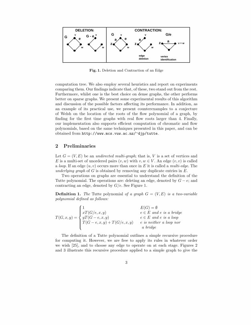
Fig. 1. Deletion and Contraction of an Edge
computation tree. We also employ several heuristics and report on experimentscomparing them. Our findings indicate that, of these, two stand out from the rest.Furthermore, whilst one is the best choice on dense graphs, the other performsbetter on sparse graphs. We present some experimental results of this algorithmand discussion of the possible factors affecting its performance. In addition, asan example of its practical use, we present counterexamples to a conjectureof Welsh on the location of the roots of the flow polynomial of a graph, byfinding for the first time graphs with real flow roots larger than 4. Finally,our implementation also supports efficient computation of chromatic and flowpolynomials, based on the same techniques presented in this paper, and can beobtained from http://www.mcs.vuw.ac.nz/∼djp/tutte.
2 Preliminaries
Let G = (V, E) be an undirected multi-graph; that is, V is a set of vertices andE is a multi-set of unordered pairs (v, w) with v, w ∈ V . An edge (v, v) is calleda loop. If an edge (u, v) occurs more than once in E it is called a multi-edge. Theunderlying graph of G is obtained by removing any duplicate entries in E.
Two operations on graphs are essential to understand the definition of theTutte polynomial. The operations are: deleting an edge, denoted by G − e; andcontracting an edge, denoted by G/e. See Figure 1.
Definition 1. The Tutte polynomial of a graph G = (V, E) is a two-variablepolynomial defined as follows:
T (G, x, y) =
1 E(G) = ∅xT (G/e, x, y) e ∈ E and e is a bridgeyT (G − e, x, y) e ∈ E and e is a loopT (G − e, x, y) + T (G/e, x, y) e is neither a loop nor
a bridge
The definition of a Tutte polynomial outlines a simple recursive procedurefor computing it. However, we are free to apply its rules in whatever orderwe wish [25], and to choose any edge to operate on at each stage. Figures 2and 3 illustrate this recursive procedure applied to a simple graph to give the
3
y
x
2y2x x2x
x x
1
2
3
5
6
7 8
11
12
13
14 x15 18 20
17 194
10 16
9
y xyyx x
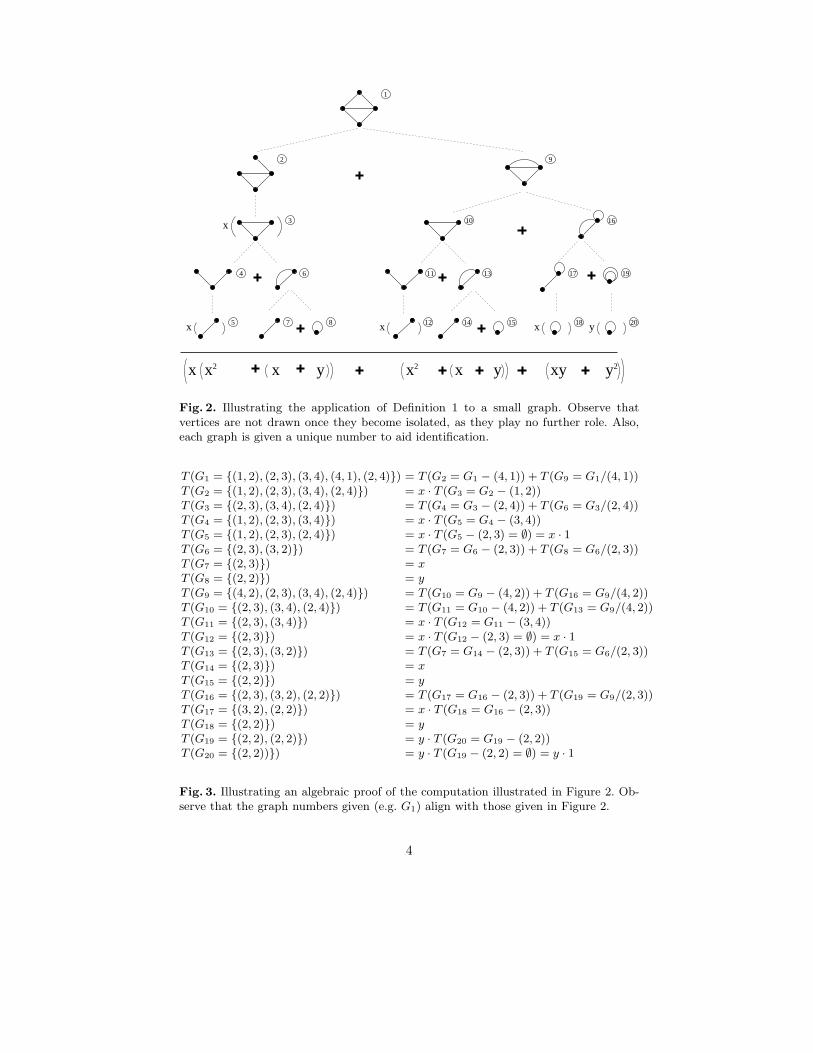
Fig. 2. Illustrating the application of Definition 1 to a small graph. Observe thatvertices are not drawn once they become isolated, as they play no further role. Also,each graph is given a unique number to aid identification.
T (G1 = {(1, 2), (2, 3), (3, 4), (4, 1), (2, 4)}) = T (G2 = G1 − (4, 1)) + T (G9 = G1/(4, 1))T (G2 = {(1, 2), (2, 3), (3, 4), (2, 4)}) = x · T (G3 = G2 − (1, 2))T (G3 = {(2, 3), (3, 4), (2, 4)}) = T (G4 = G3 − (2, 4)) + T (G6 = G3/(2, 4))T (G4 = {(1, 2), (2, 3), (3, 4)}) = x · T (G5 = G4 − (3, 4))T (G5 = {(1, 2), (2, 3), (2, 4)}) = x · T (G5 − (2, 3) = ∅) = x · 1T (G6 = {(2, 3), (3, 2)}) = T (G7 = G6 − (2, 3)) + T (G8 = G6/(2, 3))T (G7 = {(2, 3)}) = xT (G8 = {(2, 2)}) = yT (G9 = {(4, 2), (2, 3), (3, 4), (2, 4)}) = T (G10 = G9 − (4, 2)) + T (G16 = G9/(4, 2))T (G10 = {(2, 3), (3, 4), (2, 4)}) = T (G11 = G10 − (4, 2)) + T (G13 = G9/(4, 2))T (G11 = {(2, 3), (3, 4)}) = x · T (G12 = G11 − (3, 4))T (G12 = {(2, 3)}) = x · T (G12 − (2, 3) = ∅) = x · 1T (G13 = {(2, 3), (3, 2)}) = T (G7 = G14 − (2, 3)) + T (G15 = G6/(2, 3))T (G14 = {(2, 3)}) = xT (G15 = {(2, 2)}) = yT (G16 = {(2, 3), (3, 2), (2, 2)}) = T (G17 = G16 − (2, 3)) + T (G19 = G9/(2, 3))T (G17 = {(3, 2), (2, 2)}) = x · T (G18 = G16 − (2, 3))T (G18 = {(2, 2)}) = yT (G19 = {(2, 2), (2, 2)}) = y · T (G20 = G19 − (2, 2))T (G20 = {(2, 2))}) = y · T (G19 − (2, 2) = ∅) = y · 1
Fig. 3. Illustrating an algebraic proof of the computation illustrated in Figure 2. Ob-serve that the graph numbers given (e.g. G1) align with those given in Figure 2.
4
final polynomial. It should be clear from these figures that the structure of thecomputation corresponds to a tree.
The order in which the rules of Definition 1 are applied significantly affects thesize of the computation tree. An “efficient” order can reduce work in a numberof ways. For example, there are two situations where an edge is associated witha factor directly: if the edge is a loop, the factor is y; likewise, if the edge is abridge, the factor is x. Eliminating such edges as soon as possible and storingthe factor for later incorporation into the answer reduces work by lowering thecost of operations (e.g. contracting, connectedness testing, etc.) on graphs in thesubtrees below. In Figure 2, for example, the loop present in G16 is not reducedimmediately and, instead, is propagated to the bottom of the computation tree;removing it immediately reduces, amongst other things, the cost of duplicatingthe graph when the branch forks further down.
Within a single computation tree, it often arises that a graph G occurs morethan once. Thus, recomputing T (G) from scratch each time is wasteful andshould be avoided when possible. For example, the triangle occurs twice in Figure2, both as G3 and G10. Thus, we can simplify the tree by simply reusing theresult from T (G3) in place of T (G10). This optimisation has a significant effecton the performance of our algorithm in practice (as shown in §6).
The choice of edge for a delete/contract operation can also greatly affect thesize of the computation tree. In particular, it affects the likelihood of reaching agraph isomorphic to one already seen. For example, selecting (4, 2) when evalu-ating T (G9) in Figure 3 yields the triangle (as shown); choosing any of the otheredges, however, does not. We have not yet explored the effects of different edgeselection heuristics, although this remains important future work.
Finally, an efficient algorithm for computing Tutte polynomials can be usedimmediately to compute chromatic, flow and reliability polynomials. For ex-ample, for the chromatic polynomial P (G, λ) and flow polynomial F (G, x) of agraph with n vertices, e edges and c connected components are derived as followsfrom the Tutte polynomial:
P (G, λ) = (−1)n−cλ · T (G, (1 − λ), 0)
F (G, x) = (−1)e−n+c · T (G, 0, (1 − x))
3 Roots of Flow Polynomials - Welsh’s Conjecture
Our primary motivation for developing an efficient algorithm was to extendthe range for which computational exploration of questions relating to Tuttepolynomials is feasible, as there are a number of long-standing open questionsfor which our computational evidence is extremely limited.
Several of these problems relate to the location of the roots of the varioussingle-variable specialisations of the Tutte polynomial mentioned earlier. In par-ticular, the roots of the chromatic polynomial, or chromatic roots have beenextensively studied while much less is known about the roots of the flow poly-nomial. One fundamental question about which very little is known is whether
5
there is an upper bound on the value of real flow roots. As there are graphs(such as the Petersen graph) with no 4-flows, the strongest possible result wouldbe that there are no real flow roots larger than 4.
Conjecture 1 (Dominic Welsh) If G is a bridgeless graph with flow polyno-mial FG, then FG(r) > 0 for all r ∈ (4,∞).
This conjecture is essentially a dual version of the famous Birkhoff-Lewisconjecture that planar graphs have no chromatic roots in [4,∞) which has beenproved for r = 4 (the four-colour theorem) and for [5,∞).
In prior study of chromatic roots, cubic graphs of high girth have played animportant role as they seem to exhibit qualitatively extremal behaviour (thisis a deliberately imprecise statement) and for this reason, they are a naturalclass to examine for other questions related to Tutte polynomials. In this veinwe computed the Tutte polynomials of cubic graphs of girth at least 7 on 24–32vertices with the intention of testing a variety of conjectures against this dataset.
An immediate positive outcome of this experiment was the discovery of anumber of counterexamples to Welsh’s conjecture. A specific example is thegeneralised Petersen graph P (16, 6) which is a 32-vertex cubic graph of girth 7shown in Figure 4 with flow polynomial (t − 1)(t − 2)(t − 3)Q(t) where
Q(t) = t14 − 42 t13 + 833 t12 − 10358 t11 + 90393 t10 − 587074 t9
+ 2934917 t8 − 11515364 t7 + 35798907 t6 − 88275860 t5
+ 171273551 t4 − 256034548 t3 + 282089291 t2
− 207662412 t + 77876944.
This has real roots at two values t1 ≈ 4.0252205 and t2 ≈ 4.2331455 therebydemonstrating that 4 is not the upper limit for flow roots.
There are a variety of other examples on 28 and 36 vertices, but the smallerones are more difficult to describe. The common features of the examples foundare that the flow polynomial is a polynomial of reasonably high odd degree thathas a negative derivative at t = 4 and is strongly positive at t = 5. The graphs on30 and 34 vertices that were examined have flow polynomials of even degree withpositive derivative at t = 4 and values that just keep increasing as t increases.
Given that 4 is not an upper limit for flow roots, what would be an appropri-ate replacement for Welsh’s conjecture? The nature of these examples suggeststhat they will not give flow roots above 5, and yet there seems to be no strongreason to choose any value strictly between 4 and 5. Therefore we propose thefollowing conjecture:
Conjecture 2 If G is a bridgeless graph with flow polynomial FG, then FG(r) >0 for all r ∈ [5,∞).
6
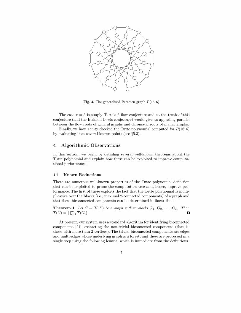
Fig. 4. The generalised Petersen graph P (16, 6)
The case r = 5 is simply Tutte’s 5-flow conjecture and so the truth of thisconjecture (and the Birkhoff-Lewis conjecture) would give an appealing parallelbetween the flow roots of general graphs and chromatic roots of planar graphs.
Finally, we have sanity checked the Tutte polynomial computed for P (16, 6)by evaluating it at several known points (see §5.3).
4 Algorithmic Observations
In this section, we begin by detailing several well-known theorems about theTutte polynomial and explain how these can be exploited to improve computa-tional performance.
4.1 Known Reductions
There are numerous well-known properties of the Tutte polynomial definitionthat can be exploited to prune the computation tree and, hence, improve per-formance. The first of these exploits the fact that the Tutte polynomial is multi-plicative over the blocks (i.e., maximal 2-connected components) of a graph andthat these biconnnected components can be determined in linear time.
Theorem 1. Let G = (V, E) be a graph with m blocks G1, G2, . . ., Gm. ThenT (G) =
∏m
i=1 T (Gi).
At present, our system uses a standard algorithm for identifying biconnectedcomponents [24], extracting the non-trivial biconnected components (that is,those with more than 2 vertices). The trivial biconnected components are edgesand multi-edges whose underlying graph is a forest, and these are processed in asingle step using the following lemma, which is immediate from the definitions.
7
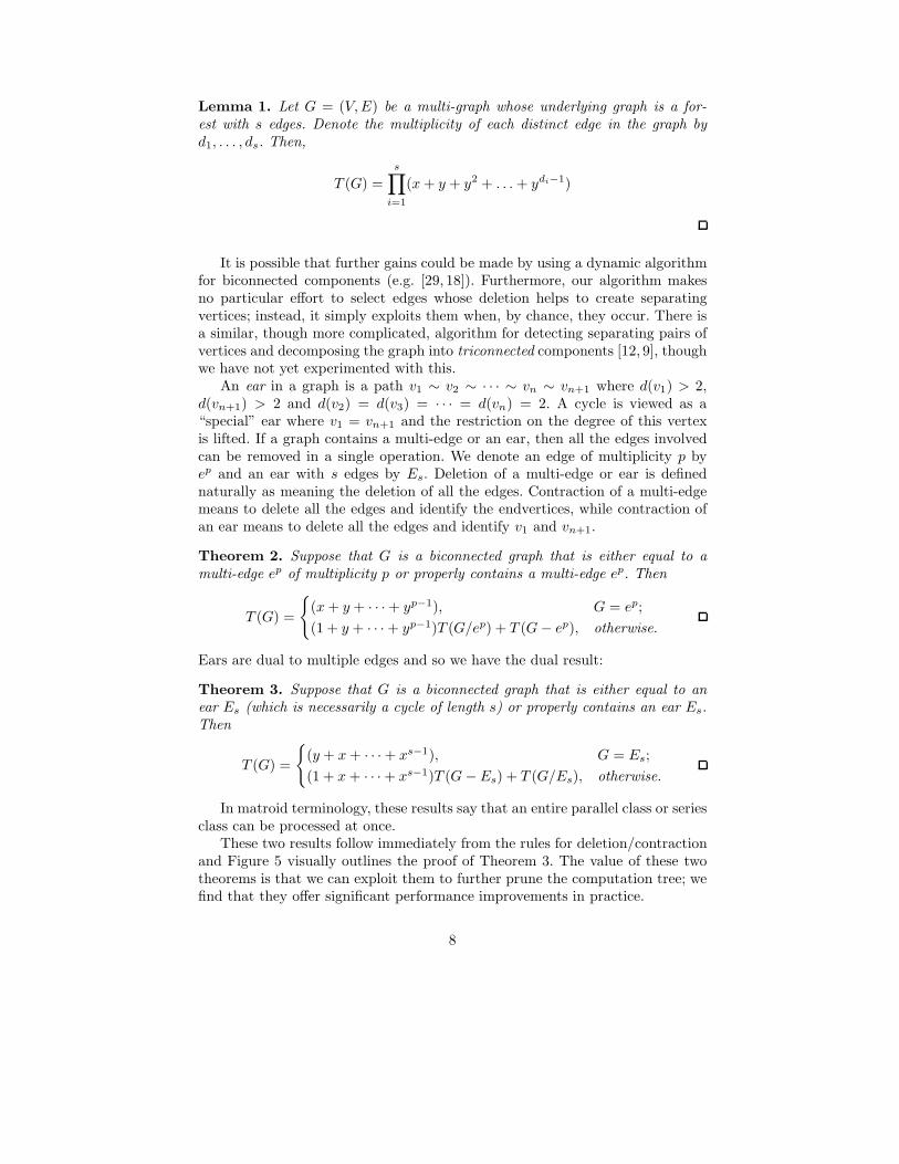
Lemma 1. Let G = (V, E) be a multi-graph whose underlying graph is a for-est with s edges. Denote the multiplicity of each distinct edge in the graph byd1, . . . , ds. Then,
T (G) =
s∏
i=1
(x + y + y2 + . . . + ydi−1)
It is possible that further gains could be made by using a dynamic algorithmfor biconnected components (e.g. [29, 18]). Furthermore, our algorithm makesno particular effort to select edges whose deletion helps to create separatingvertices; instead, it simply exploits them when, by chance, they occur. There isa similar, though more complicated, algorithm for detecting separating pairs ofvertices and decomposing the graph into triconnected components [12, 9], thoughwe have not yet experimented with this.
An ear in a graph is a path v1 ∼ v2 ∼ · · · ∼ vn ∼ vn+1 where d(v1) > 2,d(vn+1) > 2 and d(v2) = d(v3) = · · · = d(vn) = 2. A cycle is viewed as a“special” ear where v1 = vn+1 and the restriction on the degree of this vertexis lifted. If a graph contains a multi-edge or an ear, then all the edges involvedcan be removed in a single operation. We denote an edge of multiplicity p byep and an ear with s edges by Es. Deletion of a multi-edge or ear is definednaturally as meaning the deletion of all the edges. Contraction of a multi-edgemeans to delete all the edges and identify the endvertices, while contraction ofan ear means to delete all the edges and identify v1 and vn+1.
Theorem 2. Suppose that G is a biconnected graph that is either equal to amulti-edge ep of multiplicity p or properly contains a multi-edge ep. Then
T (G) =
{
(x + y + · · · + yp−1), G = ep;
(1 + y + · · · + yp−1)T (G/ep) + T (G − ep), otherwise.
Ears are dual to multiple edges and so we have the dual result:
Theorem 3. Suppose that G is a biconnected graph that is either equal to anear Es (which is necessarily a cycle of length s) or properly contains an ear Es.Then
T (G) =
{
(y + x + · · · + xs−1), G = Es;
(1 + x + · · · + xs−1)T (G − Es) + T (G/Es), otherwise.
In matroid terminology, these results say that an entire parallel class or seriesclass can be processed at once.
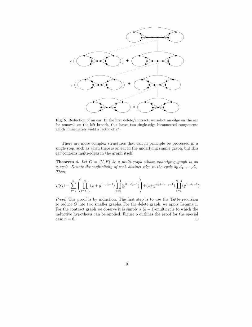
These two results follow immediately from the rules for deletion/contractionand Figure 5 visually outlines the proof of Theorem 3. The value of these twotheorems is that we can exploit them to further prune the computation tree; wefind that they offer significant performance improvements in practice.
8
x2
x
Fig. 5. Reduction of an ear. In the first delete/contract, we select an edge on the earfor removal; on the left branch, this leaves two single-edge biconnected componentswhich immediately yield a factor of x2.
There are more complex structures that can in principle be processed in asingle step, such as when there is an ear in the underlying simple graph, but thisear contains multi-edges in the graph itself.
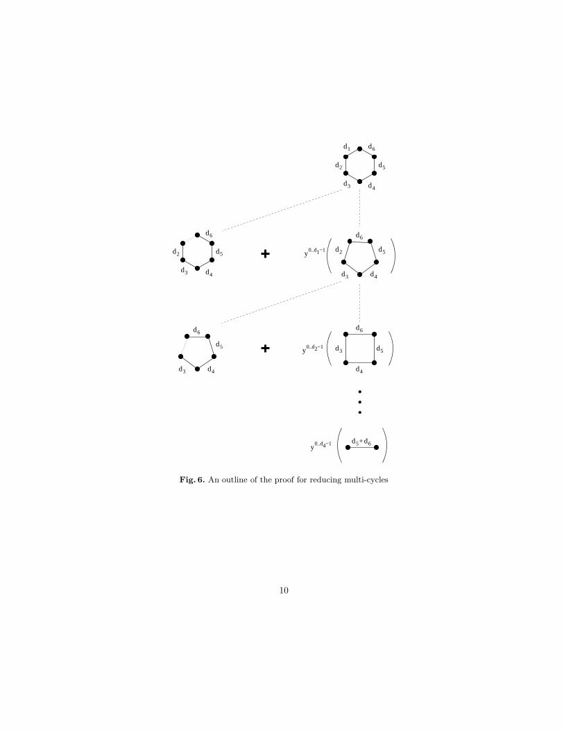
Theorem 4. Let G = (V, E) be a multi-graph whose underlying graph is ann-cycle. Denote the multiplicity of each distinct edge in the cycle by d1, . . . , dn.Then,
T (G) =
n∑
i=1
n∏
j=i+1
(x + y1...dj−1)
i−1∏
k=1
(y0...dk−1)
+(x+ydn+dn−1−1)
n−2∏
i=1
(y0...di−1)
Proof. The proof is by induction. The first step is to use the Tutte recursionto reduce G into two smaller graphs. For the delete graph, we apply Lemma 1.For the contract graph we observe it is simply a (k − 1)-multicycle to which theinductive hypothesis can be applied. Figure 6 outlines the proof for the specialcase n = 6.
9
4
d5
d6
d3
d2
d4
d5
d3
d6 d6
d3 d4
d5d2
d4
d5
d6
d3
d6
d3 d4
d5
10..d −1y
0..d −12y
d6d +50..d −14y
d1
d2
d
Fig. 6. An outline of the proof for reducing multi-cycles
10
5 Algorithm Overview
We now provide an overview of our algorithm to illustrate the main choiceswe have made. We also discuss some of the more practical, but nonethelessimportant issues which we faced when implementing our algorithm for computingTutte Polynomials.
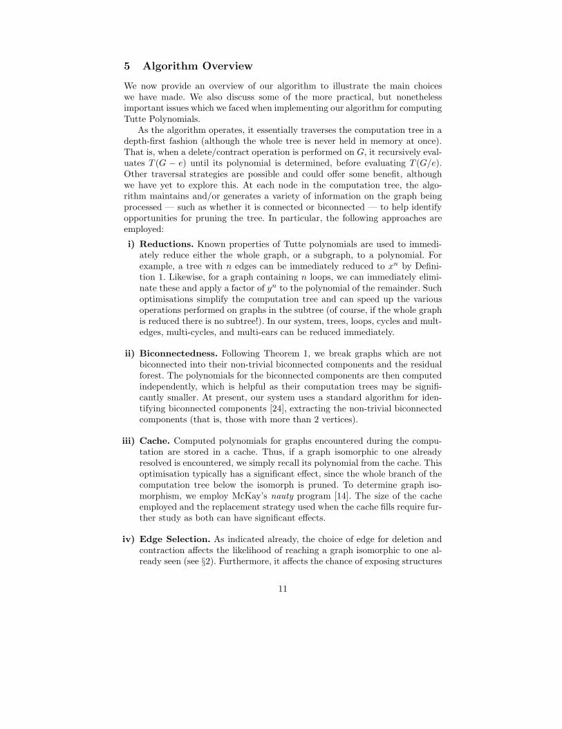
As the algorithm operates, it essentially traverses the computation tree in adepth-first fashion (although the whole tree is never held in memory at once).That is, when a delete/contract operation is performed on G, it recursively eval-uates T (G − e) until its polynomial is determined, before evaluating T (G/e).Other traversal strategies are possible and could offer some benefit, althoughwe have yet to explore this. At each node in the computation tree, the algo-rithm maintains and/or generates a variety of information on the graph beingprocessed — such as whether it is connected or biconnected — to help identifyopportunities for pruning the tree. In particular, the following approaches areemployed:
i) Reductions. Known properties of Tutte polynomials are used to immedi-ately reduce either the whole graph, or a subgraph, to a polynomial. Forexample, a tree with n edges can be immediately reduced to xn by Defini-tion 1. Likewise, for a graph containing n loops, we can immediately elimi-nate these and apply a factor of yn to the polynomial of the remainder. Suchoptimisations simplify the computation tree and can speed up the variousoperations performed on graphs in the subtree (of course, if the whole graphis reduced there is no subtree!). In our system, trees, loops, cycles and mult-edges, multi-cycles, and multi-ears can be reduced immediately.
ii) Biconnectedness. Following Theorem 1, we break graphs which are notbiconnected into their non-trivial biconnected components and the residualforest. The polynomials for the biconnected components are then computedindependently, which is helpful as their computation trees may be signifi-cantly smaller. At present, our system uses a standard algorithm for iden-tifying biconnected components [24], extracting the non-trivial biconnectedcomponents (that is, those with more than 2 vertices).
iii) Cache. Computed polynomials for graphs encountered during the compu-tation are stored in a cache. Thus, if a graph isomorphic to one alreadyresolved is encountered, we simply recall its polynomial from the cache. Thisoptimisation typically has a significant effect, since the whole branch of thecomputation tree below the isomorph is pruned. To determine graph iso-morphism, we employ McKay’s nauty program [14]. The size of the cacheemployed and the replacement strategy used when the cache fills require fur-ther study as both can have significant effects.
iv) Edge Selection. As indicated already, the choice of edge for deletion andcontraction affects the likelihood of reaching a graph isomorphic to one al-ready seen (see §2). Furthermore, it affects the chance of exposing structures
11
(e.g. cycles and trees) which can be immediately reduced. We have found thattwo edge-selection heuristics perform particularly well: vertex order and min-imising single degree. In §5.2, we provide explore these and other heuristicsin more detail.
The coefficients computed for the Tutte polynomial of even a small graphare large and can easily go beyond the size of a machines 32-bit or 64-bit wordsize. To address this, we have implemented a simple library for arbitrary sizedintegers.
5.1 Graph Isomorphism
To implement the cache for polynomials of graphs at nodes of the computationtree, we employ a simple hash map. This is keyed upon a canonical labeling ofthe graph obtained using nauty [14]. Since nauty accepts only simple graphs,we transform multigraphs into simple graphs by inserting additional vertices asnecessary. We refer to such graphs as being “constructed”. To avoid a constructedgraph from clashing with a normal simple graph having the same number ofvertices and edges, we exploit the fact that nauty allows vertices to be colouredand will reflect the colour class of a vertex in the canonical form. Thus, verticesadded to represent multi-edges are coloured differently from normal vertices. Aninteresting issue here is that, at each node in the computation tree, we mustrecompute the canonical labelling from scratch as the graph, by definition, isdifferent from its parent. While we have not explored this as yet, there is potentialfor exploiting an incremental graph isomorphism algorithm which could moreefficiently determine the canonical labelling of a graph given that of its parent.
An important problem we face is what to do when the cache fills up, whichhappens frequently for large graphs, even when large amounts (e.g. > 2GB)of memory are available. To resolve this, we employ techniques from garbagecollection: items in the cache are displaced and, to avoid memory fragmentation,those left are compacted into a contiguous block (this is similar to mark-and-sweep garbage collection). To determine which graphs to displace, we employ asimple policy based on counting the number of times a graph in the cache hasbeen “hit”. When the cache is full, graphs with a low hit count are displacedbefore those with higher counts.
Another problem is how much of the cache to displace. Clearly, displacingless means the cache will fill more frequently and, on average, contain more olditems. Of course, the more items there are in the cache, the greater the potentialfor collisions when searching for an isomorph. In contrast, displacing more of thecache each time means that many graphs which may turn out to be useful lateron will not survive. In our implementation, the default policy is to displace 30%of the cache in one go when it becomes full.
5.2 Edge-Selection Heuristics
The order in which edges are selected during the computation can have a dra-matic effect on the runtime. Here, we consider several edge-secltion heuristics
12
and identify two which perform particularly well. In the following Section, wealso provide some experimental evidence of this.
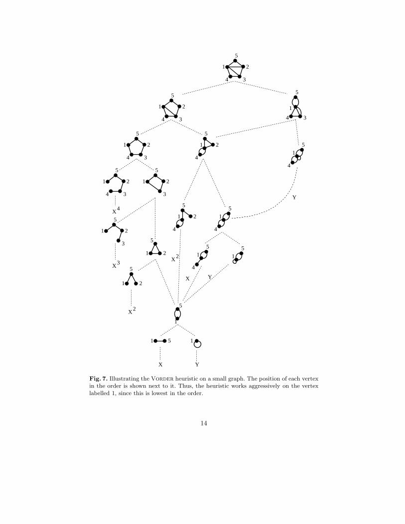
Vertex Order Heuristic. The first heuristic we consider is the vertex orderheuristic, or Vorder for short. In this heuristic, the vertices of the graph aregiven a fixed, predefined ordering. Then, as the computation proceeds, edgesare selected from the lowest vertex in the order until it becomes disconnected;once this occurs, edges are selected from the next lowest vertex until it becomesdisconnected and so on. For contractions, the resulting vertex maintains thelowest position in the order of those contracted. Furthermore, when selecting anedge for some vertex v, we choose one whose other end-point is also the lowestof any incident on v.
Figure 7 illustrates this process operating on a simple graph. In the figure,the position of each vertex in the order is shown next to it. Thus, for the firstdelete/contract, an edge from vertex 1, namely (1, 2), is selected since 1 is lowestin the ordering and 2 is below the others adjacent to 1. On the deletion side,that edge is simply removed and, thus, the next edge selected is also from 1 (thistime, it’s (1, 3); on the contract side, 1 and 2 are contracted, with the resultingvertex coming at the position previously occupied by 1 in the order.
In considering Figure 7 there is an interesting observation to make: the iso-morphic hits that occur are almost always immediately isomorphic (i.e. no per-mutation of vertices is required). To see why this is significant, let us imaginea larger graph which differs only in that some big structure is reachable fromvertex 5. Since this structure is not touched during the computation shown, weknow that the same isomorphic hits will apply. As we will see, this is not alwaysthe case for other heuristics.
From the above line of reasoning, we conclude that Vorder promotes thelikelihood of an isomorphic match occurring, and that this explains why it per-forms so well on dense graphs (as we will see in §6). Whilst studying this heuris-tic, we have also made some other observations. Firstly, contracting two verticessuch that the resultant vertex assumes the highest position of either generallydoes not perform as well. Secondly, using an ordering where vertices with higherdegree come lower in the ordering generally also gives better performance.
Degree Selection Heuristics. The second kind of heuristic we consider arethose which select edges based on their degree. The idea is to choose an edgewhich either minimises or maximises the degree in some way, and we considerhere a family of related heuristics:
– Minimise Single Degree (Minsdeg): here the edge selected at each pointin the computation tree has an end-point with the minimal degree of anyvertex.
– Minimise Degree (Mindeg): here the edge selected at each point in thecomputation has end-points whose degree sum is the least of any edge.
13
Y
X2
X3
X4
3
5
4
1 2
3
5
4
1 2
3
5
4
1 2
3
5
1 2
1
5
4 3
5
21
4
X Y
1
5
1 5 1
1
4
5
1
5
1
4
55
21
4
X2
1
4
5
3
5
1 2
1 2
5
1 2
5
3
5
4
1 2
X Y
Fig. 7. Illustrating the Vorder heuristic on a small graph. The position of each vertexin the order is shown next to it. Thus, the heuristic works aggressively on the vertexlabelled 1, since this is lowest in the order.
14
5
X2
Y3
Y2
X
X
X
X Y
X
Y
1
2 3
4
5
1
1
1
1
1
1 1
1
1 1
1
1
1
2
2
2
2 2
2
2
2
2
2 2
2
1
3
3
3
3
3
3
3
3
2
1
11
3
3
3
1
4
4
4 4
4
44
41
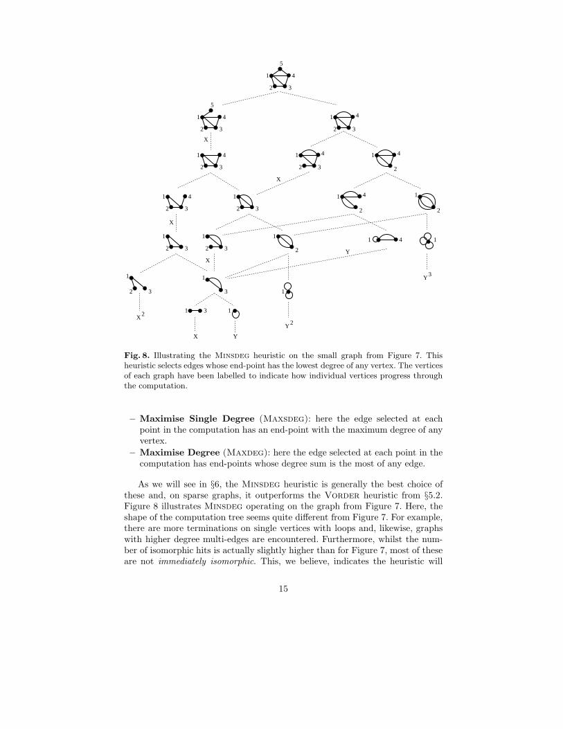
Fig. 8. Illustrating the Minsdeg heuristic on the small graph from Figure 7. Thisheuristic selects edges whose end-point has the lowest degree of any vertex. The verticesof each graph have been labelled to indicate how individual vertices progress throughthe computation.
– Maximise Single Degree (Maxsdeg): here the edge selected at eachpoint in the computation has an end-point with the maximum degree of anyvertex.
– Maximise Degree (Maxdeg): here the edge selected at each point in thecomputation has end-points whose degree sum is the most of any edge.
As we will see in §6, the Minsdeg heuristic is generally the best choice ofthese and, on sparse graphs, it outperforms the Vorder heuristic from §5.2.Figure 8 illustrates Minsdeg operating on the graph from Figure 7. Here, theshape of the computation tree seems quite different from Figure 7. For example,there are more terminations on single vertices with loops and, likewise, graphswith higher degree multi-edges are encountered. Furthermore, whilst the num-ber of isomorphic hits is actually slightly higher than for Figure 7, most of theseare not immediately isomorphic. This, we believe, indicates the heuristic will
15
not promote isomorphic matching as well as Vorder. This is because, in largergraphs, more structures will be present that prevent isomorphic hits from occur-ring until much later in the computation. For example, in Figure 8 consider theisomorphic hit that occurs between the third and fourth levels. In this case, wehave one graph with vertices {1, 2, 3} and another with vertices {1, 3, 4}. Thus, ifwe imagine computing the polynomial of a larger graph which differs by havingsome structure adjacent to vertex 4, then we can see that this isomorphic hitwould not occur. In practice, with Minsdeg, isomorphic hits typically occur atlevels which are further down the computation tree than with Vorder. Never-theless, we find that Minsdeg does outperform Vorder on sparse graphs (see§6), although the reason for this remains unclear. We believe, however, that itmay be because Minsdeg tends to promote the breaking up of cycles whichexposes large tree portions that can be automatically reduced.
5.3 Correctness
The output of any complex computer program should be treated with caution, ifnot outright suspicion, and carefully examined for internal consistency and cross-referenced against known values. Aside from manual testing on small graphs, weemploy a number of “sanity checks” to increase our confidence in its correctness.The easiest check is to compute T (G; 2, 2), which should give 2|E(G)| [4], andcompare this with a direct computation of 2|E(G)|. Another check is to computeT (G; 1, 1), which gives the number of spanning trees in the graph. Then, we cancheck that these evaluations are constant for a given graph, regardless of whatparameters are chosen for a particular run of our algorithm (e.g. cache size,which reductions are applied, edge selection strategy, vertex ordering, etc).
As an illustration, we have sanity-checked the generalised Petersen graphP (16, 6) discussed in §3 as follows:
– T (2, 2) = 248 as required.– T (1, 1) = 115184214544 is the number of spanning trees of P (16, 6) as de-
termined by the matrix-tree theorem.– (−1) T (1 − x, 0) equals the chromatic polynomial of P (16, 6) which was
independently verified by two separate programs.– T (−1,−1) = −2 equals the expected value (−2)d where d = 1 is the dimen-
sion of the bicycle space of P (16, 6) which can be computed by elementarylinear algebra.
– T (0,−3) = −480 is the number of 4-flows of P (16, 6) which is equal to thenumber of edge-3-colourings of P (16, 6) which can easily be verified by adirect search.
6 Experimental Results
In this section, we report on some experimental results obtained using our sys-tem. In particular, we look at the effect of using the isomorph cache, and the
16
edge-selection heuristics outlined in §5.2. The objective here is to give an indica-tion of the effect that these features have on performance. We consider randomconnected graphs, random 3-regular and random planar graphs. The machineused for these experiments was an Intel Pentium IV 3GHz with 1GB of memory,running NetBSD v4.99.9.
6.1 Experimental Procedure
To generate random connected graphs, we employed the tool genrang (suppliedwith nauty) to construct random graphs with a given number of edges; fromthese, we selected connected graphs until there were 100 for each value of |E| or|V | (depending upon experiment). The genrang tool constructs a random graphby generating a random edge, adding it to the graph (if not already present), andthen repeating this until enough edges have been added. We also used genrang
to generate random simple regular graphs — this essentially works by generatinga random regular multigraph and then throwing it out if it contains loops or mul-tiple edges. Generating random planar graphs required a different approach sincethe number of randomly generated graphs that are planar is extremely small.Therefore, we employed a markov-chain approach; here, an edge was selectedat random and added to the graph, provided it was not already present andthe graph remained planar; otherwise, it was removed — again, provided thatthe graph remained planar. This procedure was repeated for 3n2 steps (which,according to [6], is well beyond the equilibrium point).
6.2 Experimental Results
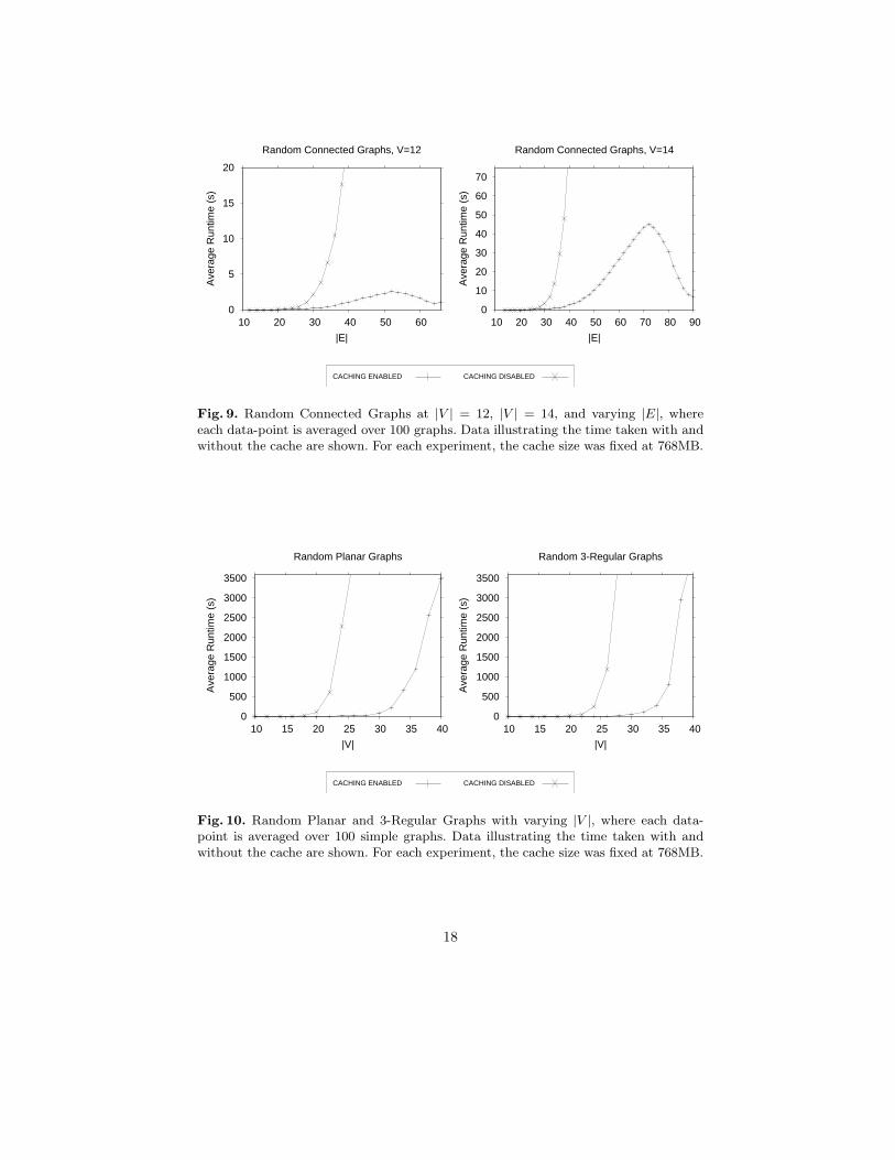
Figure 9 presents the data from our experiments on random connected graphs.Data is provided for timings with and without the cache enabled. From the fig-ure, it is immediately obvious that the cache has a critical effect on the perfor-mance of the algorithm. As expected, performance deteriorates as graph densityincreases; however, the algorithm appears to perform surprisingly well on verydense graphs. This stems from the increased regularity present in dense graphswhich gives rise to a greater number of isomorphic hits in the cache.
Figure 10 reports the data from our experiments on random planar and3-regular. From the graphs, it is clear that computing the Tutte polynomial forlarge graphs quickly becomes intractable. Nevertheless, using the isomorphismcache extends the size of graphs which can be computed. This is of significantvalue in practice, since it extends the range of graphs over which users of thetool can, for example, test a conjecture they are considering.
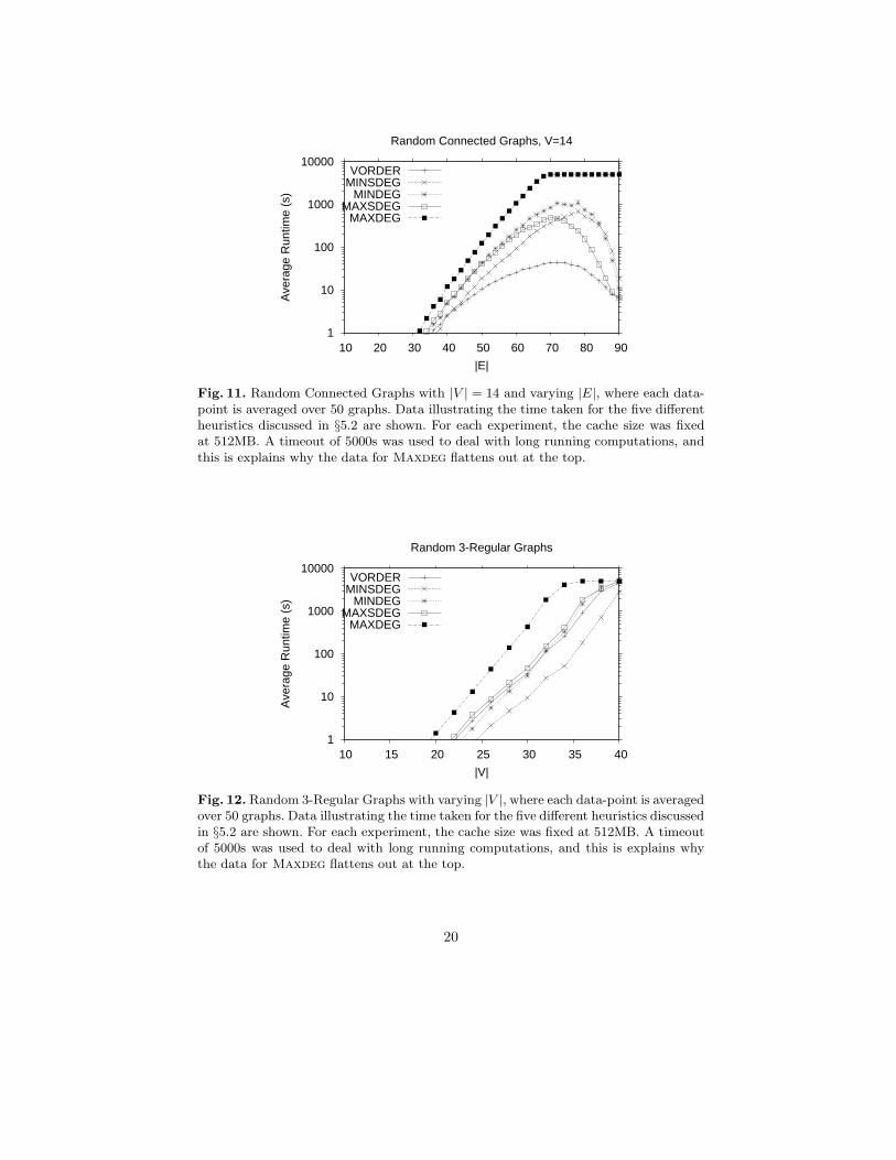
Figure 11 presents the data from our experiments on random connectedgraphs. Data is provided for each of the five heuristics, and observe that a logscale is used on the y-axis. Also, a timeout of 5000s was used to deal with longrunning computations, and this is explains why the data for Maxdeg flattensout at the top. From the figure, it is immediately obvious that the Vorderheuristic performs particularly well compared with the others. The reason forthis, we believe, is that it promotes the chance of reaching a graph which is
17
0
5
10
15
20
10 20 30 40 50 60
Ave
rage
Run
time
(s)
|E|
Random Connected Graphs, V=12
0
10
20
30
40
50
60
70
10 20 30 40 50 60 70 80 90
Ave
rage
Run
time
(s)
|E|
Random Connected Graphs, V=14
CACHING DISABLEDCACHING ENABLED
Fig. 9. Random Connected Graphs at |V | = 12, |V | = 14, and varying |E|, whereeach data-point is averaged over 100 graphs. Data illustrating the time taken with andwithout the cache are shown. For each experiment, the cache size was fixed at 768MB.
0
500
1000
1500
2000
2500
3000
3500
10 15 20 25 30 35 40
Ave
rage
Run
time
(s)
|V|
Random Planar Graphs
0
500
1000
1500
2000
2500
3000
3500
10 15 20 25 30 35 40
Ave
rage
Run
time
(s)
|V|
Random 3-Regular Graphs
CACHING DISABLEDCACHING ENABLED
Fig. 10. Random Planar and 3-Regular Graphs with varying |V |, where each data-point is averaged over 100 simple graphs. Data illustrating the time taken with andwithout the cache are shown. For each experiment, the cache size was fixed at 768MB.
18
isomorphic to one already seen. Note, very dense graphs tend to be easier tosolve, since their increased regularity leads to a greater number of isomorphichits in the cache.
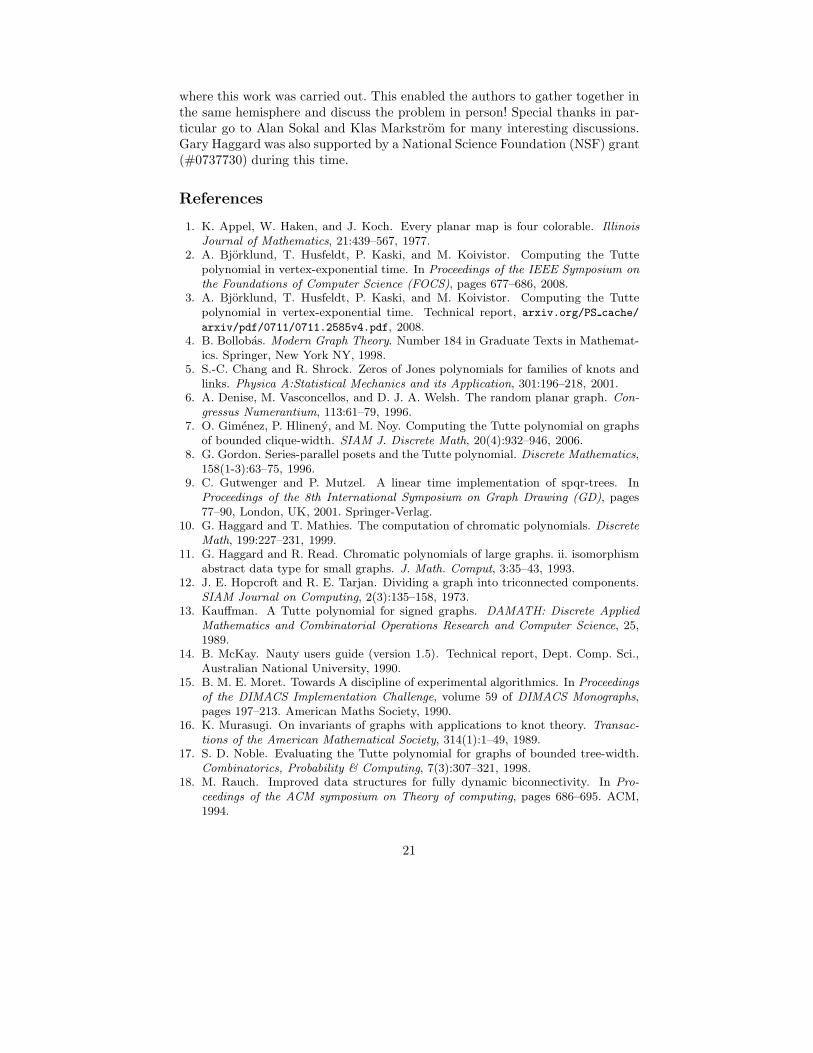
Figure 12 reports the data from our experiments on random 3-regular and4-regular graphs. Data is provided for each of the five heuristics, and observethat a log scale is used on the y-axis. For the 3-regular graphs, we can see thatthe Minsdeg heuristic gives a significant performance benefit over the others.However, on the 4-regular graphs (which are denser) we see the gap betweenMinsdeg and Vorder closes. Furthermore, it is fairly evident that computingthese graphs is considerably more expensive than for the 3-regular graphs.
7 Conclusion
Algorithms for computing Tutte polynomials have been, in general, rather sim-plistic. We have demonstrated a number of techniques which can greatly reducethe size of the computation tree. This, in turn, leads to an algorithm which cantackle significantly larger graphs than previously possible. While this task mayseem futile (since the problem is #P-Hard), it is important to remember that,in practice, the applications of this tool (e.g. for classifying DNA knots) havefinite requirements; thus, we are moving towards a system which can handlesufficiently large graphs to be of use to practitioners.
A number of interesting questions remain for further research. Firstly, theedge-selection heuristics we have explored seem rather simple; can we identifyother heuristics which lead to even better selection orders? Secondly, at eachnode in the computation tree, we compute a canonical labelling of the corre-sponding graph so it can be stored in the cache (this enables later identificationof isomorphs). But, should we do this at every node? For example, could wemaintain the canonical labelling incrementally? Thirdly, can we strengthen thetermination conditions? For example, computing the Chromatic polynomial ofa complete graph is very easy. Thus, for dense graphs, it makes more sense tomove towards complete graphs than empty graphs. Indeed, we have trialled thisfor computing chromatic polynomials with considerable success. However, it’sunclear how this can be applied to the general Tutte computation.
Nevertheless, even with this list of interesting unanswered questions, theimplementation described gives researchers an effective and efficient way to ex-periment with Tutte polynomials both to answer questions and test conjecturesfor a wide range of sizes of graphs [15]. The complete implementation of our al-gorithm can be obtained from http://www.mcs.vuw.ac.nz/∼djp/tutte. Thisalso supports efficient computation of chromatic and flow polynomials, based onthe same techniques presented in this paper.
Acknowledgements. We wish to thank the Isaac Newton Institute for Math-ematical Sciences, University of Cambridge, for generous support during theprogramme on Combinatorics and Statistical Mechanics (January – June 2008),
19
1
10
100
1000
10000
10 20 30 40 50 60 70 80 90
Ave
rage
Run
time
(s)
|E|
Random Connected Graphs, V=14
VORDERMINSDEG
MINDEGMAXSDEG
MAXDEG
Fig. 11. Random Connected Graphs with |V | = 14 and varying |E|, where each data-point is averaged over 50 graphs. Data illustrating the time taken for the five differentheuristics discussed in §5.2 are shown. For each experiment, the cache size was fixedat 512MB. A timeout of 5000s was used to deal with long running computations, andthis is explains why the data for Maxdeg flattens out at the top.
1
10
100
1000
10000
10 15 20 25 30 35 40
Ave
rage
Run
time
(s)
|V|
Random 3-Regular Graphs
VORDERMINSDEG
MINDEGMAXSDEG
MAXDEG
Fig. 12. Random 3-Regular Graphs with varying |V |, where each data-point is averagedover 50 graphs. Data illustrating the time taken for the five different heuristics discussedin §5.2 are shown. For each experiment, the cache size was fixed at 512MB. A timeoutof 5000s was used to deal with long running computations, and this is explains whythe data for Maxdeg flattens out at the top.
20
where this work was carried out. This enabled the authors to gather together inthe same hemisphere and discuss the problem in person! Special thanks in par-ticular go to Alan Sokal and Klas Markstrom for many interesting discussions.Gary Haggard was also supported by a National Science Foundation (NSF) grant(#0737730) during this time.
References
1. K. Appel, W. Haken, and J. Koch. Every planar map is four colorable. IllinoisJournal of Mathematics, 21:439–567, 1977.
2. A. Bjorklund, T. Husfeldt, P. Kaski, and M. Koivistor. Computing the Tuttepolynomial in vertex-exponential time. In Proceedings of the IEEE Symposium onthe Foundations of Computer Science (FOCS), pages 677–686, 2008.
3. A. Bjorklund, T. Husfeldt, P. Kaski, and M. Koivistor. Computing the Tuttepolynomial in vertex-exponential time. Technical report, arxiv.org/PS cache/
arxiv/pdf/0711/0711.2585v4.pdf, 2008.4. B. Bollobas. Modern Graph Theory. Number 184 in Graduate Texts in Mathemat-
ics. Springer, New York NY, 1998.5. S.-C. Chang and R. Shrock. Zeros of Jones polynomials for families of knots and
links. Physica A:Statistical Mechanics and its Application, 301:196–218, 2001.6. A. Denise, M. Vasconcellos, and D. J. A. Welsh. The random planar graph. Con-
gressus Numerantium, 113:61–79, 1996.7. O. Gimenez, P. Hlineny, and M. Noy. Computing the Tutte polynomial on graphs
of bounded clique-width. SIAM J. Discrete Math, 20(4):932–946, 2006.8. G. Gordon. Series-parallel posets and the Tutte polynomial. Discrete Mathematics,
158(1-3):63–75, 1996.9. C. Gutwenger and P. Mutzel. A linear time implementation of spqr-trees. In
Proceedings of the 8th International Symposium on Graph Drawing (GD), pages77–90, London, UK, 2001. Springer-Verlag.
10. G. Haggard and T. Mathies. The computation of chromatic polynomials. DiscreteMath, 199:227–231, 1999.
11. G. Haggard and R. Read. Chromatic polynomials of large graphs. ii. isomorphismabstract data type for small graphs. J. Math. Comput, 3:35–43, 1993.
12. J. E. Hopcroft and R. E. Tarjan. Dividing a graph into triconnected components.SIAM Journal on Computing, 2(3):135–158, 1973.
13. Kauffman. A Tutte polynomial for signed graphs. DAMATH: Discrete AppliedMathematics and Combinatorial Operations Research and Computer Science, 25,1989.
14. B. McKay. Nauty users guide (version 1.5). Technical report, Dept. Comp. Sci.,Australian National University, 1990.
15. B. M. E. Moret. Towards A discipline of experimental algorithmics. In Proceedingsof the DIMACS Implementation Challenge, volume 59 of DIMACS Monographs,pages 197–213. American Maths Society, 1990.
16. K. Murasugi. On invariants of graphs with applications to knot theory. Transac-tions of the American Mathematical Society, 314(1):1–49, 1989.
17. S. D. Noble. Evaluating the Tutte polynomial for graphs of bounded tree-width.Combinatorics, Probability & Computing, 7(3):307–321, 1998.
18. M. Rauch. Improved data structures for fully dynamic biconnectivity. In Pro-ceedings of the ACM symposium on Theory of computing, pages 686–695. ACM,1994.
21
19. R. Read. An improved method for computing chromatic polynomials of sparsegraphs. Technical Report CORR 87-20, Dept. Comb. & Opt., University of Wa-terloo, 1987.
20. G. F. Royle. Computing the Tutte polynomial of sparse graphs. Technical ReportCORR 88-35, Dept. Comb. & Opt., University of Waterloo, 1988.
21. K. Sekine, H. Imai, and S. Tani. Computing the Tutte polynomial of a graph ofmoderate size. Lecture Notes in Computer Science, 1004:224–233, 1995.
22. A. D. Sokal. The multivariate Tutte polynomial (alias Potts model) for graphsand matroids. In Surveys in combinatorics 2005, volume 327 of London Math.Soc. Lecture Note Ser., pages 173–226. Cambridge Univ. Press, Cambridge, 2005.
23. A. D. Sokal. The multivariate Tutte polynomial (alias Potts model) for graphsand matroids. In Surveys in combinatorics 2005, volume 327 of London Math.Soc. Lecture Note Ser., pages 173–226. Cambridge Univ. Press, Cambridge, 2005.
24. R. E. Tarjan. Depth-first search and linear graph algorithms. SIAM Journal onComputing, 1(2):146–160, 1972.
25. W. Tutte. A contribution to the theory of chromatic polynomials. CanadianJournal of Mathematics, 6:80–81, 1954.
26. Vertigan. The computational complexity of Tutte invariants for planar graphs.SICOMP: SIAM Journal on Computing, 35, 2006.
27. D. Welsh. The Tutte polynomial. Random Structures Algorithms, 15(3-4):210–228, 1999. Statistical physics methods in discrete probability, combinatorics, andtheoretical computer science (Princeton, NJ, 1997).
28. D. J. A. Welsh and C. Merino. The Potts model and the Tutte polynomial. Journalof Mathematical Physics, 41(3):1127–1152, 2000.
29. J. Westbrook and R. Tarjan. Maintaining bridge-connected and biconnected com-ponents on-line. Algorithmica, 7(1):433–464, 1992.
22