Computing the shapeof flexible shafts

Thomas ten Cate

Institute for Mathematicsand Computing Science

Bachelor thesis

Computing the shapeof flexible shafts

Thomas ten Cate

Supervisors:A.E.P. Veldman and H. BekkerUniversity of GroningenInstitute for Mathematics and Computing ScienceP.O. Box 8009700 AV GroningenThe Netherlands May 2007

Abstract

This thesis concerns the shape of �exible shafts or rods in three dimensions, whose position andderivative are constrained at the endpoints, but whose length is allowed to change freely. Thisproblem has a practical application in drill heads made by the customer, Koese Engineering.

Two models are presented based on the physical aspects of the system. The �rst modelis more elegant and more widely applicable; the second was developed speci�cally for thecustomer's particular situation.

Neither system of equations can be solved analytically. A combination of several numericalalgorithms is used to compute the shape of a shaft under absolute precision requirements.

Finally, the design and development of a software program is presented that allows thecustomer to quickly enter his data and extract the results.

6

7

Contents

1 Introduction 9

1.1 Objectives . . . . . . . . . . . . . . . . . . . . . . . . . . . . . . . . . . . . . . . 91.2 Outline . . . . . . . . . . . . . . . . . . . . . . . . . . . . . . . . . . . . . . . . 10

2 Geometric model 11

2.1 Description of a drill head . . . . . . . . . . . . . . . . . . . . . . . . . . . . . . 112.2 Geometric model . . . . . . . . . . . . . . . . . . . . . . . . . . . . . . . . . . . 12

3 Model of a bending shaft 17

3.1 Parametrisation along the shaft . . . . . . . . . . . . . . . . . . . . . . . . . . . 173.1.1 Boundary conditions . . . . . . . . . . . . . . . . . . . . . . . . . . . . . 173.1.2 Elastic bending . . . . . . . . . . . . . . . . . . . . . . . . . . . . . . . . 183.1.3 Forces and moments . . . . . . . . . . . . . . . . . . . . . . . . . . . . . 193.1.4 Di�erential equations . . . . . . . . . . . . . . . . . . . . . . . . . . . . . 20

3.2 Parametrisation in z . . . . . . . . . . . . . . . . . . . . . . . . . . . . . . . . . 213.2.1 Boundary conditions . . . . . . . . . . . . . . . . . . . . . . . . . . . . . 213.2.2 Di�erential equations . . . . . . . . . . . . . . . . . . . . . . . . . . . . . 213.2.3 The circular arc . . . . . . . . . . . . . . . . . . . . . . . . . . . . . . . . 22

4 Algorithms 25

4.1 Algorithm overview . . . . . . . . . . . . . . . . . . . . . . . . . . . . . . . . . . 254.2 Error metric . . . . . . . . . . . . . . . . . . . . . . . . . . . . . . . . . . . . . . 264.3 Numerical integration . . . . . . . . . . . . . . . . . . . . . . . . . . . . . . . . 26

4.3.1 Integration step size . . . . . . . . . . . . . . . . . . . . . . . . . . . . . 274.4 Solving for the parameters . . . . . . . . . . . . . . . . . . . . . . . . . . . . . . 284.5 Interpolation . . . . . . . . . . . . . . . . . . . . . . . . . . . . . . . . . . . . . 28

5 Requirements 31

5.1 Functional requirements . . . . . . . . . . . . . . . . . . . . . . . . . . . . . . . 315.2 Nonfunctional requirements . . . . . . . . . . . . . . . . . . . . . . . . . . . . . 32

6 User interface design 33

6.1 Menu bar . . . . . . . . . . . . . . . . . . . . . . . . . . . . . . . . . . . . . . . 336.2 Main dimensions . . . . . . . . . . . . . . . . . . . . . . . . . . . . . . . . . . . 346.3 Side view . . . . . . . . . . . . . . . . . . . . . . . . . . . . . . . . . . . . . . . 356.4 Top view . . . . . . . . . . . . . . . . . . . . . . . . . . . . . . . . . . . . . . . . 35

8 CONTENTS

6.4.1 Top bearings . . . . . . . . . . . . . . . . . . . . . . . . . . . . . . . . . 366.4.2 Shafts . . . . . . . . . . . . . . . . . . . . . . . . . . . . . . . . . . . . . 376.4.3 Guiding block holes . . . . . . . . . . . . . . . . . . . . . . . . . . . . . 376.4.4 Support bearing holes . . . . . . . . . . . . . . . . . . . . . . . . . . . . 37

7 Technical design 39

7.1 Language and tools . . . . . . . . . . . . . . . . . . . . . . . . . . . . . . . . . . 397.2 Overview of software structuring . . . . . . . . . . . . . . . . . . . . . . . . . . 40

7.2.1 Maths . . . . . . . . . . . . . . . . . . . . . . . . . . . . . . . . . . . . . 407.2.2 Model . . . . . . . . . . . . . . . . . . . . . . . . . . . . . . . . . . . . . 407.2.3 GUI . . . . . . . . . . . . . . . . . . . . . . . . . . . . . . . . . . . . . . 417.2.4 Tests . . . . . . . . . . . . . . . . . . . . . . . . . . . . . . . . . . . . . . 42

8 Tests and Results 43

8.1 Comparison to the circle . . . . . . . . . . . . . . . . . . . . . . . . . . . . . . . 438.2 Comparison to accurate computations . . . . . . . . . . . . . . . . . . . . . . . 438.3 Real-world tests . . . . . . . . . . . . . . . . . . . . . . . . . . . . . . . . . . . . 46

9 Conclusion 49

A Pseudocode algorithms 53

A.1 The Broyden algorithm . . . . . . . . . . . . . . . . . . . . . . . . . . . . . . . 53

9

Chapter 1

Introduction

Koese Engineering [1] is a company whose core business is the manufacturing of drills forindustrial purposes. These drills are speci�cally designed for high-speed production, typicallytaking only a few seconds to drill dozens of holes at once.

Koese specialises in drilling many closely-spaced holes in one go.Because the distance between the holes is often smaller than theholes themselves, there is no room for gearwheels to drive each drillseparately. Koese's patented solution for this problem is to drivethe drills using �exible shafts that bend outwards from the blockcontaining the drills, creating space for a large gearwheel in the centrethat drives all shafts.

The �exible shafts will bend when pressure is put onto the drills.If a shaft bends too much, it will break. Therefore the shafts aresupported at a few points (typically one to three) by a bronze platewith holes in it through which the shafts run.

1.1 Objectives

For years, Koese has constructed the aforementioned bronze plates simply by putting theshafts in the right position and then measuring where the holes in the bronze plates neededto be. This is a very time-consuming task.

The objective of this project is to analyse the problem mathematically and come up with away to compute the positions of these holes in advance. To easily use the resulting algorithm,a computer program will be written that performs the necessary computations numerically.This program will have a graphical user interface that facilitates easy input and readout ofdata.

A secondary objective is to make the program into a useful aid when deciding upon thedimensions of the machine. The important factor here is the minimum bending radius thatoccurs in any shaft, because this corresponds to maximum curvature and therefore the highestprobability of breaking.

10 CHAPTER 1. INTRODUCTION

1.2 Outline

We will start in chapter 2 by describing and modelling the situation. This chapter is relevantfor all other chapters, so it should be read carefully.

The next two chapters are primarily of interest to the mathematically oriented reader.The equations necessary for computing the shaft shapes will be derived in chapter 3. Thealgorithms for numerically solving the equations are treated in chapter 4.

Three chapters on the development of the program follow; these are obviously primarilyintended for readers from the �eld of computing science, most notably software engineering.The requirements are discussed in chapter 5. Chapter 6 presents the design of the user interfacebased upon these requirements, and chapter 7 discusses the implementation of this interfaceand the underlying algorithms.

Test results acquired with this program are given in chapter 8, leading up to the conclusionin chapter 9.

11

Chapter 2

Geometric model

The �rst section of this chapter, section 2.1, describes in detail how a Koese drill head isbuilt up physically. In section 2.2 this is then translated into the mathematical domain byconstructing a geometrical interpretation.

2.1 Description of a drill head

We will describe the structure of a Koese drill head from bottom to top. (Without loss ofgenerality, we can assume that the machine drills holes downward. Most Koese machines dothis, but it is not a requirement.) The word drill head in this context means everything theproject is involved with, and so does not include, for example, the engine that drives themachine or the supports it is standing on.

Refer to �gure 2.1 for an overview picture of a drill head designed to drill 18 holes at once.

At the bottom, there is the product to be drilled. Above that, the drills protrude from theguiding block, which is simply a block of metal with holes in it to guide the drills. The drillscan slide freely through the guiding block in the axial (vertical) direction.

From the top of the guiding block the �exible shafts emerge. Their direction is initiallyexactly vertical, but they bend away from each other as we get higher up. In the following,when the word �shaft� is used without further speci�cation, the �exible shaft is meant.

Along the way up, a shaft runs through the holes in a number of bronze plates calledsupport bearings, mounted horizontally to support the shafts.

Where the �exible shaft ends at the top, it changes into a normal, rigid shaft, runningfurther upwards, but not exactly vertical. The angle between the rigid shaft and the verticalis typically in the order of 10 degrees, and equal for all shafts. Sometimes there is no rigidshaft, but we model this by simply setting its length to zero.

At the top end of the rigid shaft, it is supported by a ball bearing called the top bearing

(to distinguish it from the support bearing mentioned before). Somewhere along the rigidshaft, a small gearwheel is mounted. The rigid shafts are placed in such a way that thesegearwheels are on a circle. In the centre of this circle is a large gearwheel, that drives thesmall gearwheels on all rigid shafts simultaneously.

12 CHAPTER 2. GEOMETRIC MODEL

Figure 2.1: A Koese drill head with 18 shafts and one support bearing.

2.2 Geometric model

In this section, the coordinate system will be described and several important constants willbe introduced that are used throughout the rest of the document.

As we are not concerned with the drills or the guiding block at the bottom, we place theorigin of our coordinate system at the top of the guiding block, where the �exible shafts start.The z-axis runs upward from there, whereas the x-axis can be thought of to run to the rightand the y-axis to the back. A side view in the direction of the positive y-axis is given in �gure2.2.

H is the height of the drill head, measured along the z-axis, but note that this includesonly the part with the �exible shafts.

α is the angle between the rigid shaft and the z-axis, and is therefore called the rigid shaft

angle. It also determines the tangent at the top of the �exible shaft.

R is the so-called pure bending radius of the shafts. It follows from H and α, becauseR = H/ sinα. If the shape of a shaft follows a circle, which indeed does happen in the`ideal' case as we will see later, then R is the radius of this circle.

2.2. GEOMETRIC MODEL 13

Figure 2.2: A schematic model of a drill head. One shaft is shown that lies in the xz-plane.

x is the fan radius, and can be computed as x = R − R cos α. It is the distance betweenthe bottom and the top of a circular arc, projected onto the xy-plane, and thereforeamounts to the space gained by using �exible shafts.

L is the length of the rigid shaft. It is 0 in case there are no rigid shafts.

r is the so-called average radius. It is not actually any average in the strict sense. Thename `average radius' was chosen because r is usually chosen such that it is close tothe average distance of a hole to the origin, in order to minimise the distance from thebottom of a shaft to the circle de�ned by r.

h is the height of a support bearing, measured to its centre. We discuss all support bearingsindependently of each other, so an index (e.g. h1, h2) is not needed.

a is the thickness of a support bearing.

db is the diameter of the top bearings, again equal for all bearings.

ds is the diameter of the �exible shaft, and can be assumed to be equal for all �exibleshafts. It also determines the size of the holes in the support bearing.

dd is the diameter of the drills, and therefore also of the drilled holes.

14 CHAPTER 2. GEOMETRIC MODEL

Figure 2.3: The drill head model seen from the top. The rigid shaft and top bearing are notshown.

The top view is shown in �gure 2.3. Here we see a shaft that does not lie in the xz-plane.Note that r and r + x sweep out a circle. The tops of the �exible shafts are all on the circlewith radius r + x.

β is the angle between the x-axis and the tangent vector at the top of the shaft. It isdi�erent for each shaft. In practical situations, the shafts are often equally spaced, e.g.β = 0◦, 15◦, 30◦, . . ..

Where the shaft intersects a support bearing, it does so at a certain point (x, y, h) in acertain direction, de�ned in the spherical coordinates seen in �gure 2.4.

γ is the azimuth at the point of intersection, de�ned to be the counterclockwise angle fromthe x-axis to the projection of the tangent vector onto the xy-plane.

δ is the elevation1 at the point of intersection, which is the angle between the tangent andthe z-axis.

1The terms `azimuth' and `elevation' are borrowed from astronomy. However, in astronomy the word`elevation' usually refers to the angle between the vector and the xz-plane.

2.2. GEOMETRIC MODEL 15

Figure 2.4: A shaft intersecting a support bearing.

16

17

Chapter 3

Model of a bending shaft

In order to determine the placement of the holes in a support bearing, we need to know theshape that a given shaft will assume. In this section, physical modelling will be used to resultin a set of non-linear di�erential equations that describe the shape of the shaft, given theposition and tangent at its endpoints.

The required system of di�erential equations is essentially derived in [2], and section 3.1is mostly a rephrasing of this derivation. The result is a six-dimensional system. However, forthis speci�c purpose, it turns out to be possible to reduce this to a four dimensional system,at the cost of slightly more complex equations. This result is presented in section 3.2.

3.1 Parametrisation along the shaft

We describe the shape of the shaft as a curve c of length Lb in three-dimensional space:

c : [0, Lb] −→ R3,

c : t 7−→

x(t)y(t)z(t)

.

Because t parametrises the length along the shaft, the derivative of c with respect to t musthave magnitude 1:

‖c′(t)‖ =√

x′(t)2 + y′(t)2 + z′(t)2 = 1. (3.1)

3.1.1 Boundary conditions

In order to �t into the drill head, certain conditions on c must be satis�ed. The start and endpositions are �xed, as is the direction (tangent, or simply �rst derivative) at the start and endpoint. If the hole to be drilled is at (bx, by), then observing �gures 2.2 and 2.3 and applying

18 CHAPTER 3. MODEL OF A BENDING SHAFT

some trigonometry, we get the following boundary conditions:

c(0) =

bx

by

0

, c(Lb) =

(r + x) cos β(r + x) sinβ

H

,

c′(0) =

001

, c′(Lb) =

sinα cos βsinα sinβ

cos α

.

(3.2)

Note that the length Lb of the shaft is not known.

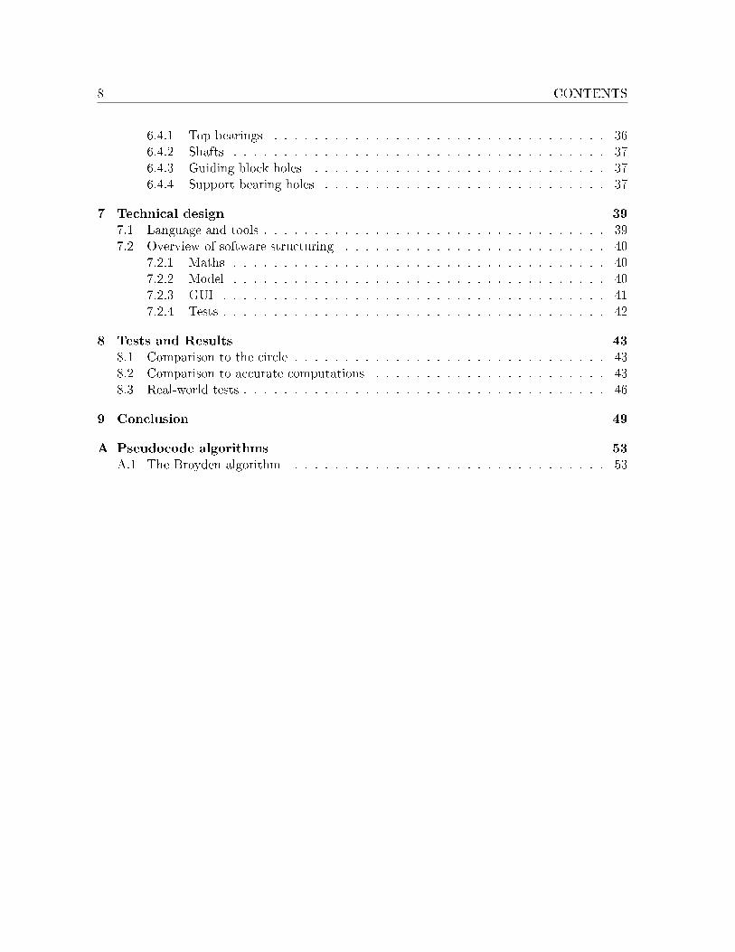
3.1.2 Elastic bending

The shaft takes on the shape that it does because forces and bending moments are exertedon it. We assume that the shaft is very thin compared to its length, that its cross section isconstant and that it is made of a uniform material. All of these assumptions hold very well inpractice. This allows us to use the Bernoulli-Euler equation1, that is often used in engineeringdisciplines, as the basic model of bending:

K(t) = −M(t)EI

. (3.3)

Here, M(t) is the bending moment of the shaft at a the point c(t), and K(t) is the curvature,here de�ned as

K(t) =c′(t)× c′′(t)‖c′(t)‖3

= c′(t)× c′′(t). (3.4)

Note that both M and K are vectors. E and I are physical parameters (the elasticity modulusand the moment of inertia, respectively). However, these do not in�uence the shape of theshaft, so we set both to 1, resulting in

K(t) = −M(t). (3.5)

Because ‖c′(t)‖ = 1 by (3.1), we know that c′ does not change in magnitude. This impliesthat the second derivative c′′(t) is perpendicular to c′(t) at every point:

c′(t) · c′′(t) =

x′(t)y′(t)z′(t)

· x′′(t)

y′′(t)z′′(t)

= x′(t)x′′(t) + y′(t)y′′(t) + z′(t)z′′(t)

=ddt

(12x′(t)2 +

12y′(t)2 +

12z′(t)2)

=12

ddt

(x′(t)2 + y′(t)2 + z′(t)2)

=12

ddt

1

= 0.

1In the literature, this equation is often found in di�erent forms, for example in two dimensions andparametrised in the x-coordinate. The equation is presented here in its most generic form, working in eithertwo or three dimensions and not constraining one spatial coordinate to be a function of another.

3.1. PARAMETRISATION ALONG THE SHAFT 19

To `invert' the cross product (3.4), we use the following lemma: if p = q × r and q ⊥ r,then ‖q‖2r = p × q. The proof is neither di�cult nor interesting and can be found in theliterature. Filling in p = K(t), q = c′(t) and r = c′′(t), and using ‖c′(t)‖ = 1, gives us

c′′(t) = K(t)× c′(t),

and combining with (3.4) yields:

c′′(t) = −M(t)× c′(t) = c′(t)×M(t). (3.6)

3.1.3 Forces and moments

We imagine that the shaft is �rst �xed at the top (that is, at the bottom of the rigid shaft)and allowed to �oat freely. Barring gravity, it will of course be straight. To force the shaftinto its desired position, a force and bending moment are exerted on the bottom of the shaft,where it intersects the z = 0 plane; see �gure 3.1. Note that the eventual length of the shaftis not known: it is allowed to shift freely at the bottom in the z direction.

Figure 3.1: The forces and moments acting on the shaft.

The force is split into scalar components Fx and Fy. There is no force in the z direction,because it is assumed that no pressure is being put on the drills. Similarly, the moment is

20 CHAPTER 3. MODEL OF A BENDING SHAFT

split into Mx0 and My0. There is no moment around the z-axis because there is no torsionbeing applied to the drills. At this point, Fx, Fy, Mx0 and My0 are unknown. These need tobe chosen in such a way that the bottom of the shaft ends up in the desired position with thedesired tangent.

The bending moment `felt' at a point c(t) along the shaft is the sum of the moment atthe bottom and the moment resulting from the force applied at the bottom. The momentresulting from this force is found by multiplying the force with the length of its lever arm,which is equal to z(t) in this case. This results in a non-zero moment around the z-axis aswell; see again �gure 3.1.

From this, taking care to get the signs correct, and leaving out the dependency on t forreadability, we deduce that the moment acting on any part of the shaft is given by

M =

Mx

My

Mz

=

Mx0 + zFy

My0 − zFx

(y − by)Fx − (x− bx)Fy

. (3.7)

3.1.4 Di�erential equations

Plugging (3.7) into (3.6), we �nd x′′

y′′

z′′

=

y′Mz − z′My

z′Mx − x′Mz

x′My − y′Mx

=

y′((y − by)Fx − (x− bx)Fy)− z′(My0 − zFx)z′(Mx0 + zFy)− x′((y − by)Fx − (x− bx)Fy)

x′(My0 − zFx)− y′(Mx0 + zFy)

.

This is a three-dimensional system of second-order ordinary di�erential equations. It canbe rewritten to a six-dimensional system of �rst-order ordinary di�erential equations in thestandard way:

ddtx = x′,ddty = y′,ddtz = z′,ddtx

′ = y′((y − by)Fx − (x− bx)Fy)− z′(My0 − zFx),ddty

′ = z′(Mx0 + zFy)− x′((y − by)Fx − (x− bx)Fy),ddtz

′ = x′(My0 − zFx)− y′(Mx0 + zFy).

These equations contain the four unknowns Fx, Fy, Mx0 and My0. In the boundaryconditions (3.2) a �fth unknown, the length of the shaft Lb, is stated. It would appear thatwe are dealing with a system of �ve variables and six constraints, yet it turns out to have asolution. The reason is that the sixth constraint is satis�ed automatically because of (3.1):our solution is parametrised in the length along the shaft. Therefore, if the end conditions forx′ and y′ are satis�ed, then, by (3.1), so is the end condition for z′.

In general, it is not possible to solve these equations analytically. An approach to a numeri-cal solution is brie�y described in [2]; however, matters are complicated by the extra constraint(3.1) and the fact that the integration length Lb is unknown. In the next section, a simplersystem is derived which has only four dimensions and no constraint on the parametrisation,and eliminates Lb entirely.

3.2. PARAMETRISATION IN Z 21

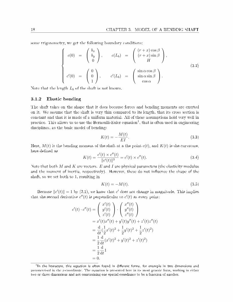
3.2 Parametrisation in z

Because in practical situations, a shaft will never `double back' onto itself, it is safe to assumethat every plane perpendicular to the z-axis is intersected at most once. In other words, theshape of the shaft can also be seen as a function mapping a z-coordinate between 0 and H toits corresponding x- and y-coordinates. For consistency, we retain the third coordinate z butkeep in mind that this is simply the identity function:

c : [0,H] −→ R3,

c : z 7−→

x(z)y(z)z

.

Also note

c′(z) =

x′(z)y′(z)z′(z)

=

x′(z)y′(z)

1

, c′′(z) =

x′′(z)y′′(z)z′′(z)

=

x′′(z)y′′(z)

0

,

and therefore

‖c′(z)‖ =√

x′(z)2 + y′(z)2 + 1,

which is no longer constant as in (3.1). This renders some of its corollaries invalid.

3.2.1 Boundary conditions

The boundary conditions (3.2) take on a di�erent form in the new parametrisation, which canagain easily be derived with some trigonometry:

c(0) =

bx

by

0

, c(H) =

(r + x) cos β(r + x) sinβ

H

,

c′(0) =

001

, c′(H) =

tanα cos βtanα sinβ

1

.

(3.8)

3.2.2 Di�erential equations

The Bernoulli-Euler equation (3.3) remains intact, because both K and M are reparametrised.The curvature K, however, can no longer be written in the elegant form of (3.4), but instead

22 CHAPTER 3. MODEL OF A BENDING SHAFT

becomes

K(z) =c′(z)× c′′(z)‖c′(z)‖3

=c′(z)× c′′(z)

(x′(z)2 + y′(z)2 + 1)32

= (x′(z)2 + y′(z)2 + 1)−32

y′(z)z′′(z)− z′(z)y′′(z)z′(z)x′′(z)− x′(z)z′′(z)x′(z)y′′(z)− y′(z)x′′(z)

= (x′(z)2 + y′(z)2 + 1)−

32

−y′′(z)x′′(z)

x′(z)y′′(z)− y′(z)x′′(z)

.

Combining this with K(z) = −M(z) from (3.5) and plugging in M from (3.7) gives us

(x′(z)2 + y′(z)2 + 1)−32

−y′′(z)x′′(z)

x′(z)y′′(z)− y′(z)x′′(z)

= −

Mx0 + zFy

My0 − zFx

(y − by)Fx − (x− bx)Fy

.

This can again be rewritten into a system di�erential equations, by solving it for y′′ andz′′. We do not need the third component, so we leave it out on both sides.

ddtx = x′,ddty = y′,ddtx

′ = (−My0 + zFx)(x′(z)2 + y′(z)2 + 1)32 ,

ddty

′ = (Mx0 + zFy)(x′(z)2 + y′(z)2 + 1)32 .

(3.9)

These are the �nal di�erential equations that will be used in the program. The four unknownparameters are Fx, Fy, Mx0 and My0. The integration length is now known to be H and thereare no secondary constraints.

These equations are not known to be analytically solvable. They can easily be linearised byneglecting the x′(z) and y′(z) terms, which will be small in practical cases. The linear systemcan then be solved analytically and results in a third-degree polynomial for both x and y. Thisis one of the approaches taken in [2] to estimate the maximum curvature, producing resultswith an error of a few percent.

For this application however, a more precise result is required. Therefore, the nonlinearsystem will have to be solved using numerical methods, which are described in the next chapter.First, however, we will discuss a situation which does allow an exact solution.

3.2.3 The circular arc

As might be expected from the law of conservation of energy, in this case bending energy, theshaft will prefer a shape with as little bending as possible. If its constraints allow, it will takeon the shape of a perfectly circular arc. In this section we will show that this is indeed asolution of the aforementioned equations.

For simplicity, we assume that the shaft is in the xz-plane, to the right of the z axis, likethe one in �gure 2.2. This assumption is equivalent to β = 0. The proof can be extended to

3.2. PARAMETRISATION IN Z 23

the general case, but this only leads to more complex computations without delivering anymore insights. Such a circular shaft in the xz plane is described by

x(z) = r + R−√

R2 − z2,

y(z) = 0.

To allow a perfectly circular shape, the boundary conditions need to be just right. This isrealised by setting

bx = r,

by = 0.

See again �gure 2.2.The y part is trivial: everything remains 0 everywhere. We will therefore focus on the x

part. We start by di�erentiating:

x′(z) =z√

R2 − z2.

Now we can check without much di�culty that the boundary conditions in (3.8) are indeedsatis�ed.

To verify that x conforms to the di�erential equations (3.9) we di�erentiate x′ again, usingthe product rule:

x′′(z) =1√

R2 − z2+

z2

(R2 − z2)32

=1√

R2 − z2

(z2

R2 − z2+ 1)

=1R

√R2

R2 − z2

(z2

R2 − z2+ 1)

=1R

(z2

R2 − z2+ 1) 1

2(

z2

R2 − z2+ 1)

=1R

(z2

R2 − z2+ 1) 3

2

.

Now we note that z2

R2−z2 = x′(z)2 and 0 = y′(z)2, so we get

x′′(z) =1R

(x′(z) + y′(z) + 1

) 32 .

To make this satisfy (3.9), we choose My0 = − 1R and Fx = 0, resulting in

x′′(z) = (−My0 + zFx)(x′(z) + y′(z) + 1

) 32 ,

which proves that a circular arc is indeed a solution.

24

25

Chapter 4

Algorithms

Eventually, the customer is interested in two things: the placement of the holes in a supportbearing, and the minimum bending radius of a shaft. For estimating the minimum bendingradius, a simple formula has been produced [2] which works very well in practice. The focus ofthis project will therefore be on computing the positions of the holes in the support bearings,and the angle under which these need to be drilled. These values correspond to x(h), y(h),x′(h) and y′(h) in the modelling of section 3.2.

4.1 Algorithm overview

If the values of the four parameters Fx, Fy, Mx0 and My0 are given, then equations (3.9)can be solved using numerical integration. This will give the position and tangent at certainpoints along the shaft, and in particular at the top end of the shaft, z = H. The numericalintegration is discussed in detail in section 4.3.

We then need to determine the values of the four parameters such that these positionand tangent match those of the boundary conditions (3.8). Essentially, we are dealing with afunction

S : R4 −→ R4,

S : (Fx, Fy,Mx0,My0) 7−→ (x(H), y(H), x′(H), y′(H)),

where the value of S is determined by the numerical integration process, and we want to solve

S(Fx, Fy,Mx0,My0) = (xe, ye, x′e, y

′e), (4.1)

where xe, ye, x′e, y′e are the constants from the boundary condition (3.8) at H. This solvingcan be done with an o�-the-shelf algorithm. This algorithm is discussed in section 4.4.

Note that the combination of a numerical integrator and an equation solver results in whatis essentially a so-called `shooting method': �re a `shot' for certain values of the parameters,see where we end up, adjust the parameters and try again, until the shot is on (or close enoughto) the target.

Once the values of these parameters have been determined we can run the numericalintegration one more time to get a list of points along the shaft. In general there will be no

26 CHAPTER 4. ALGORITHMS

Figure 4.1: A schematic overview of the algorithm that computes the shaft shape.

point at exactly the height h where we want to determine the values of x, y, x′ and y′, so wewill need some form of interpolation. This is treated in section 4.5.

Figure 4.1 gives a schematic overview of the algorithm discussed above.

4.2 Error metric

Numerical computations like this will never be precisely accurate. A way to measure the errorin the result is needed. As an error metric, we will use the Euclidian distance between thereal location (x∗(h), y∗(h), h) and the computed location (x(h), y(h), h) of the hole. Both areat a height of z = h, so this distance is computed in the horizontal plane. Given a value forthe tolerance τ , we want to achieve the following:√

(x(h)− x∗(h))2 + (y(h)− y∗(h))2 ≤ τ.

In practice, τ will be around 0.1 mm for H in the order of 103 mm. It is possible to de�ne τas a percentage of H if desired.

Rather arbitrarily, we use the same measure and the same τ for the derivative. Thisprovides our second constraint:√

(x′(h)− x∗′(h))2 + (y′(h)− y∗′(h))2 ≤ τ.

4.3 Numerical integration

The most well-known and very frequently used algorithm for solving �rst-order ordinary dif-ferential equations is the fourth-order Runge-Kutta (RK4) method [3, p. 278], which seemslike a good choice at �rst sight.

However, the RK4 algorithm uses a �xed step size which has to be speci�ed in advance.This may not be a good idea if we want precise control over the error. The adaptive Runge-Kutta-Fehlberg (RKF) method [3, pp. 285�286], on the other hand, incorporates a minimumand a maximum step size, and will adaptively adjust the actual step size used. This step sizeis based on an estimate of the local truncation error, produced by running an RK4 and anRK5 method side by side.

On the other hand, the di�erential equations that we are dealing with are quite smooth,and derivatives are relatively small. Experiments with RKF revealed that it nearly alwaysdecides to use the maximum allowed step size. The extra overhead produced by the RK5method is therefore worthless. For this reason, eventually RK4 was chosen for the numericalintegration procedure.

4.3. NUMERICAL INTEGRATION 27

Figure 4.2: A sketch to determine the step size for the numerical integration.

4.3.1 Integration step size

For determining an appropriate step size for the RK4 algorithm, we assume that the resultingpoints are on a circle. In practice they will indeed be close to a circular arc. We furtherassume that they are interpolated in a linear fashion, which, as we will see later, is a worst-case scenario.

Now we can use �gure 4.2 to determine the maximum step size. Because the points aredistributed evenly on the z-axis, the largest error will occur at the top, in the last segment,where the slope of the shaft is largest with respect to the z axis. Because this is precisely theerror that we want to control, we call this distance τ . We assume that the largest error occursclose to the midpoint of the segment, as can be seen in the �gure, so we de�ne m as half thelength of this segment. We de�ne τ⊥ to be the distance from the midpoint to the circle.

From the Pythagorean theorem, followed by some trigonometry, we get:

τ⊥ = R−√

R2 −m2

= R−√

R2 − (R sin ξ)2

= R−R

√1− sin2 ξ.

Solving for ξ yields:

ξ = asin

√2τ cos α

R− τ2 cos2 α

R2.

Some more trigonometry gives us h:

h = R sinα−R sin(α− 2ξ),

28 CHAPTER 4. ALGORITHMS

into which we can plug in ξ to produce

h = R sinα−R sin

(α− 2 asin

√2τ cos α

R− τ2 cos2 α

R2

),

which is the step size to use for the RK4 algorithm.

4.4 Solving for the parameters

Now that we have a way to map the four parameters Fx, Fy, Mx0 and My0 to the resultingsituation at the endpoint x(H), y(H), x′(H), y′(H), we need a way to solve the nonlinear sys-tem of equations (4.1), thereby sending the endpoint towards its desired position. A numericalequation solver has to be used here.

Because the derivative of S is unknown, Newton's method is useless here. (Note that evenS itself cannot be written analytically, because it is the result of a numerical process.) In one-dimensional systems this problem can be solved by using the secant method. There exists ageneralization of the secant method to higher dimensions, known as Broyden's method. Pleaserefer to A.1 for the pseudocode of this algorithm. Instead of requiring the exact derivative(Jacobian matrix), it employs an estimate, which is updated in each iteration. Broyden'salgorithm is the one that we will use.

The algorithm given in [3] was slightly modi�ed to be able to meet absolute precisionrequirements, in terms of τ , instead of stopping as soon as the change in the result dropsbelow a certain threshold. For details, again see A.1.

In Step 9 of this algorithm, a matrix A is updated using a term multiplied by 1p . However,

the algorithm does not mention what to do in case p = 0. One case where p can become 0 iswhen the �rst estimate is already correct. This happened in one of the unit tests, where theshape of a straight shaft along the z-axis is computed. Skipping the update of A is a correctapproach for these situations, but might not handle cases where p becomes 0 for some otherreason. As the book [3] does not mention anything about this, it will probably be very rareor even impossible.

As the error in the endpoint of the RK4 output will usually be an ascending function ofthe integration length z, we could assume that the largest error is in the last point, wherewe can control it. If this were always true, we could control the global error by setting thetolerance of the Broyden algorithm to τ , resulting in errors less than τ everywhere else alongthe shaft. However, sometimes the largest error turns out to be somewhere else. Because inpractice the algorithm turns out to converge very fast, we can a�ord to set its tolerance to τ

10 .This should ensure that the Broyden solver does not become the precision bottleneck of thealgorithm.

4.5 Interpolation

The series of points resulting from the numerical integration in section 4.3 can be interpolatedin a piecewise linear fashion, that is, with straight line segments between the points. However,the curve that represents the shape of a shaft is very smooth. It can therefore be expectedthat an interpolation using some form of polynomial will yield much more accurate results.

4.5. INTERPOLATION 29

A Hermite spline is a commonly used method of interpolating data points where the deriva-tive is known in every point. Some confusion exists over the precise de�nition of �Hermitespline�; we will therefore use the more concise term �piecewise cubic spline�. Because the nu-merical integration process produces a numerical value for the derivative in every point, usingpiecewise cubic interpolation is the obvious choice. To each interval between two points, a cu-bic polynomial (four degrees of freedom) is �tted that matches the values and the derivativesin both endpoints (four constraints). Unlike many other spline �tting algorithms, the inter-polation in one interval does not depend on any information outside its interval, making thisinterpolation very robust. The linearised version of the problem also produces a third-orderpolynomial as the solution (see section 3.2.2 and [2]), further supporting the choice for a cubicinterpolating function.

Cubic splines are usually created in two dimensions, but they can easily be extended tothree dimensions by working in the xz and yz projection planes and producing polynomialsfor x(z) and y(z) separately.

Because a support bearing has a certain thickness, the question remains whether to com-pute the hole position at the top, in the centre or at the bottom of the bearing. The arbitrarychoice has been made to compute the position and angle in the centre of the bearing, therebyde�ning a cilindrical hole. The curvature of the shaft over this relatively short distance isneglected.

30

31

Chapter 5

Requirements

By this point, an algorithm has been developed that can be used to compute the positionsof the holes that need to be drilled in the support bearings. The next step is to design aprogram that allows the user to work e�ciently with this algorithm. This chapter highlightsthe requirements that the program must meet, along with the reason that these requirementswere posed.

The requirements are labelled. These labels are referred to in the subsequent sections ondesign.

5.1 Functional requirements

The end goal of the program is to produce a view on the pattern of holes to be drilled in thesupport bearings. For this, the following data are needed:

FR1 � the main dimensions of the drill head,

FR2 � the location (and diameter) of the holes to be drilled,

FR3 � the location (and diameter) of the top bearings,

FR4 � the assignment between shafts and holes,

FR5 � the diameter of shafts,

FR6 � the location and thickness of the support bearings.

The UI must allow the user to input each of these. (The diameters in braces are not strictlynecessary, but are included to give the user a more complete view of the situation, to preventcreating overlapping holes or top bearings.)

The UI must be able to produce a view of the output, consisting of the patterns of holesin each of the support bearings, in three formats:

FR7 � on-screen in a graphical form, to check whether everything �looks okay�,

FR8 � printable in a tabular form, to input the data manually into some machine,

32 CHAPTER 5. REQUIREMENTS

FR9 � digital in AutoCAD DXF format [4], to be imported into a CAD program likeSolidWorks [5].

Finally, the program must support the following auxiliary features, needed to be able touse the program e�ciently:

FR10 � saving a design to a �le and loading it back from the �le,

FR11 � con�guring the tolerance τ as described before.

5.2 Nonfunctional requirements

Below is a selection of the most important nonfunctional requirements for the program, alongwith their rationale.

NFR12 � Because the program will be used on an irregular basis, and will often not beused for months, the interface must have a high degree of (re)discoverability.

NFR13 � The user interface must respond quickly to the user's actions to keep the userfrom performing the action again.

NFR14 � Incorrect output will result in lost time, money and e�ort because an incorrectsupport bearing will be produced. The utmost care should be taken to avoidthis.

NFR15 � The program must run on an average Windows XP machine as is used by KoeseEngineering.

33

Chapter 6

User interface design

In this chapter, the graphical user interface (UI) of the program is described in some detail,and the rationale behind this design is presented.

In general, the user (an employee of Koese Engineering) will have a �xed hole pattern thatneeds to be drilled, as speci�ed by the customer of Koese Engineering. This pattern will ingeneral be the �rst input of the program, and will not often be modi�ed later. The otherinputs may follow in any order.

It may be sensible to construct the interface in such a way that the hole pattern is input�rst, and is not easy to modify later on. This approach would result in a less clutteredinterface, because the controls to change the hole pattern will be hidden, but this also meansthat parts of the user interface are hidden at any point. This makes the UI less discoverable(NFR12 ), and therefore the decision was made to put all controls into a single window. Theuser can then immediately see what's available.

The most intuitive way to specify a hole pattern (FR2 ), top bearings (FR3 ), shaft assign-ments (FR4 ) and support bearings (FR6 ) is visually. The �rst three can best be done in atop view of the drill head; support bearings need a side view. In addition, we need a way tospecify the main dimensions (FR1 ). Although this could be done visually in a side view, thiswould result in a very nonstandard and possibly counter-intuitive control, so simple numericaledit boxes are preferred.

The result of this approach can be seen in �gure 6.1. The main areas in this design willbe explained in detail in the following sections.

6.1 Menu bar

This is a standard menu bar as found in many (Windows and non-Windows) programs.

The File menu contains the items to create a new drill head, to load, save (FR10 ) andprint (FR8 ) drill head designs, to export the design to a DXF �le (FR9 ), and to exit theprogram.

The Edit menu only contains a Settings item, which calls up a dialog in which the shaftshape error tolerance can be con�gured (FR11 ). This is considered an `advanced' feature andthe default setting should be �ne in most cases.

The Help menu contains an item to toggle tool tips (NFR12 ) on or o� (in case the userknows the program well enough and they become annoying) and an About item displaying

34 CHAPTER 6. USER INTERFACE DESIGN

Figure 6.1: A screen shot of the �nal program, showing a drill head design in which someshafts have not yet been assigned.

information about the program. No on-line help is provided, because a printed manual willbe produced.

6.2 Main dimensions

Figure 6.2: The edit boxes used to enter the main dimensions of the drill head.

The main dimensions area (�gure 6.2) allows the user to con�gure some of the maindimensions (FR1 ). Because the �rst four of these dimensions are interdependent, the twothat are grayed out are computed automatically. It proved to be very di�cult to come upwith a design that allows the user to enter any combination of dimensions that is su�cient to

6.3. SIDE VIEW 35

compute the others, without sacri�cing usability.

The labels H, R etcetera are used to refer to the side view.

6.3 Side view

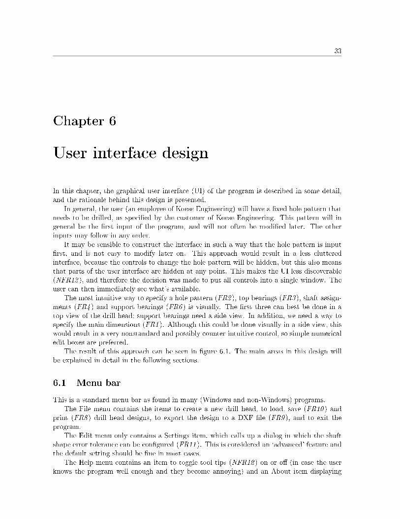
Figure 6.3: The side view of the drill head, showing two support bearings.

The side view (�gure 6.3) shows the meanings of the symbols as used in the main di-mensions area. The only manipulations that can be done in this area relate to the supportbearings.

The look and behaviour is similar to that found in many graphics and CAD programs.The side view contains a tool bar with the tools needed to manipulate the items in the view.In this case, the `arrow tool' allows support bearings to be selected and dragged up and down,the `add tool' allows creating new support bearings and the `delete tool' removes the currentlyselected bearing (FR6 ).

When a bearing is selected, the boxes at the left become available, and the height andthickness of the selected bearing can be speci�ed numerically. Moreover, selecting a bearingwill show in the top view (see section 6.4) the location of the holes in that bearing. Becausethe position of the holes is shown at the top as well as the bottom of the bearing, the sup-port bearings are drawn with a black line at the top and bottom, indicating those planes ofintersection.

6.4 Top view

As indicated before, the top view (�gure 6.4) is where most of the editing takes place. Threetypes of parts of the drill head are manipulated here: top bearings, shafts and guiding blockholes. These will be discussed in the following subsections. The controls related to the topbearings are placed at the top, those related to holes are placed at the bottom, and thoserelated to shafts are placed in the middle. This provides a subtle clue as to the purpose ofcontrols, as well as making them easier to �nd.

36 CHAPTER 6. USER INTERFACE DESIGN

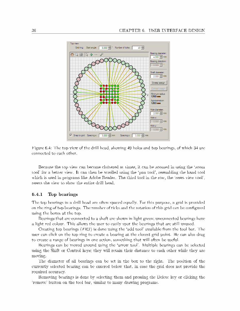
Figure 6.4: The top view of the drill head, showing 49 holes and top bearings, of which 34 areconnected to each other.

Because the top view can become cluttered at times, it can be zoomed in using the `zoomtool' for a better view. It can then be scrolled using the `pan tool', resembling the hand toolwhich is used in programs like Adobe Reader. The third tool in the row, the `reset view tool',resets the view to show the entire drill head.

6.4.1 Top bearings

The top bearings in a drill head are often spaced equally. For this purpose, a grid is providedon the ring of top bearings. The number of ticks and the rotation of this grid can be con�guredusing the boxes at the top.

Bearings that are connected to a shaft are shown in light green; unconnected bearings havea light red colour. This allows the user to easily spot the bearings that are still unused.

Creating top bearings (FR3 ) is done using the `add tool' available from the tool bar. Theuser can click on the top ring to create a bearing at the closest grid point. He can also dragto create a range of bearings in one action, something that will often be useful.

Bearings can be moved around using the `arrow tool'. Multiple bearings can be selectedusing the Shift or Control keys; they will retain their distance to each other while they aremoving.

The diameter of all bearings can be set in the box to the right. The position of thecurrently selected bearing can be entered below that, in case the grid does not provide therequired accuracy.

Removing bearings is done by selecting them and pressing the Delete key or clicking the`remove' button on the tool bar, similar to many drawing programs.

6.4. TOP VIEW 37

6.4.2 Shafts

A shaft cannot exist on its own: it is always a connection between a bearing and a hole. The`add shaft' tool (last on the tool bar) is used to create such a connection by dragging betweenthe bearing and the hole (FR4 ). An existing connection can be severed by dragging into anempty area.

Holes and bearings that are connected with a shaft are shown in green; unconnected onesare shown in red. This allows for easy checking whether the shaft assignment is complete.

Shafts themselves are coloured according to their curvature. The largest curvature in thedrill head (corresponding to the most likely point of failure) is shown in red; the smallest ingreen and intermediate values in shades ranging, via yellow, in between red and green. In thisway, the most likely point of failure can be identi�ed and improved if possible.

The diameter of all shafts can be con�gured in the box to the right (FR5 ). The shafts arenot drawn using this diameter, because that would make the top view extremely cluttered.When a support bearing is selected in the left view, however, the support bearing holes shownin the top view are drawn using this diameter (section 6.4.4).

Below this, two buttons appear that can be used to assign shafts automatically. The `sweepassign' is a heuristic currently used by Koese, which assigns top bearings to holes in the orderthey are encountered by a clock-like sweep line. The `optimal assign' should compute theoptimal shaft assignment (resulting in the smallest maximum curvature), but this function isnot (yet?) implemented and therefore the button is grayed out.

The precise value of the smallest bending radius (corresponding to the largest curvature)is shown to the right of the top view, along with a value computed using an approximationformula that has been used by Koese for years. If these numbers di�er too much, this mayindicate a potential problem (NFR14 ).

6.4.3 Guiding block holes

The holes to be drilled are shown as circles. These are added, modi�ed and removed just liketop bearings (FR2 ). They can be snapped to a grid consisting of horizontal and vertical lines,with a distance con�gurable below the top view.

Holes that have a shaft running to them are shown in bright green; those that are not yetconnected are bright red. In this way the user can easily see which holes still need attention.

The diameter of all holes can be set to the right of the view. Holes are drawn using thisdiameter.

When a hole is selected, the boxes indicating its position become available. For multipleselected holes, the box for the x-coordinate is available only if the x-coordinate is the samefor all selected holes; the same holds for the y-coordinate.

6.4.4 Support bearing holes

To avoid clutter in the top view, we do not draw all holes in support bearings in the topview. Instead, we draw only the holes in the currently selected support bearing (FR7 ). Incontrast to the internal computations, which compute the position of the hole at the centreof the bearing, the top view shows the position of the hole at the top and bottom of thebearing, with a line connecting them (�gure 6.5). This gives the user a better `feel' for the

38 CHAPTER 6. USER INTERFACE DESIGN

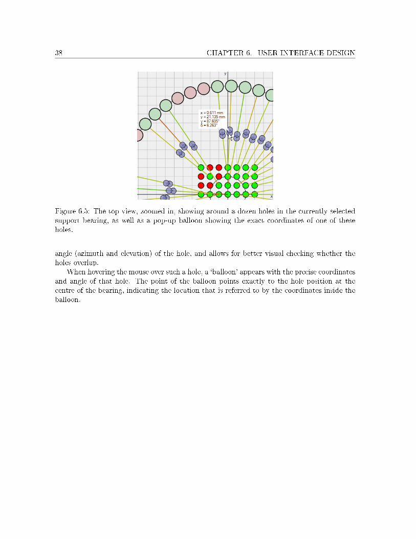
Figure 6.5: The top view, zoomed in, showing around a dozen holes in the currently selectedsupport bearing, as well as a pop-up balloon showing the exact coordinates of one of theseholes.

angle (azimuth and elevation) of the hole, and allows for better visual checking whether theholes overlap.

When hovering the mouse over such a hole, a `balloon' appears with the precise coordinatesand angle of that hole. The point of the balloon points exactly to the hole position at thecentre of the bearing, indicating the location that is referred to by the coordinates inside theballoon.

39

Chapter 7

Technical design

This chapter will discuss the overall structure of the program and elaborate on some of thedesign choices made.

7.1 Language and tools

Numerical algorithms can be implemented in nearly any programming language, and for manylanguages (most notably C) pre-built libraries exist. However, it was not clear from the startwhat the precise status of the program would be, which ruled out any library under GPL ora similar license. Implementing the algorithms by hand will give more control and should notbe too much work, given the pseudocode from the book [3]. The choice of language, therefore,need not depend on library availability.

The most important properties of a language are the speed with which code can be de-veloped, and the maintainability of the resulting code. Both considerations rule out archaiclow-level languages like C and C++, which require manual memory management and do not,for example, provide array boundary checking. This makes programming in those languagestricky, dangerous, error-prone and time-consuming. Although execution speed is not essential,because we expect the algorithms to be fast, a scripting language like Python or Perl mightbe too slow for the task. Higher level (partially) compiled languages, like Java or C#, donot su�er from these problems (NFR13 ). Java, however, has many annoyances, and C# is ingeneral a much more pleasant language in the author's humble opinion.

Another important consideration is the graphical user interface that is to be built. Imple-menting a GUI without a visual development environment will take a disproportionate amountof time and e�ort. A visual tool needs to be available for the language and toolkit used.

The program only needs to run on modern Windows systems (NFR15 ), and therefore aportable language is not needed. Indeed, portability may be bad for usability, because portableGUI toolkits usually do not employ the native Windows controls, instead re-inventing thewheel in order to roll on all platforms.

Taking into consideration the previous discussions, C# [6] was chosen as the language ofimplementation, using .NET's [7] Windows Forms1 [9] in Microsoft Visual Studio 2005 [10] toproduce the graphical user interface. For the unit tests, the logical choice is NUnit [11].

1Despite the name, a port to UNIX platforms is well under way, in the form of the Mono project [8]. Atthe time of writing, Mono is nearly complete enough to run the constructed application.

40 CHAPTER 7. TECHNICAL DESIGN

7.2 Overview of software structuring

It is nearly always a good idea to separate the frontend (user interface) from the backend(actual implementation) of the program. In this case it is essential. Without proper separationof responsibilities, it is impossible to implement automated unit tests to guarantee even a littlebit of correctness (NFR14 ) of the backend code. The backend can again be split up into two:the actual model, and the numerical algorithms. The program itself is therefore split up intothree namespaces: Maths (section 7.2.1), Model (section 7.2.2) and Gui (section 7.2.3). Afourth package, Tests (section 7.2.4), provides the unit tests and code to produce the tablesfrom section 8.

7.2.1 Maths

The Maths namespace contains all general-purpose classes for matrix algebra and numericalalgorithms.

The classes Matrix and Vector implement real-valued matrices and vectors of arbitrarydimensions. They also de�ne overloaded operators and some useful methods like Inverse andNorm.

The class Function represents an abstract function in the mathematical sense, with real-valued vectors as input and output. It has an abstract method to evaluate the function value,and implements a method to compute an approximation to the Jacobian matrix in a givenpoint. The abstract class Di�erentialEquation represents a �rst-order ordinary di�erentialequation. This is a special kind of Function where the dimension of the domain is one higher(for the time variable t) than the dimension of the codomain.

Taking a Di�erentialEquation as one of its arguments, the static method Solve in the classRK4 performs the numerical integration discussed in section 4.3.

The static method Solve in the class BroydenSolver uses the algorithm from section 4.4 tosolve F (x) = 0 for a certain Function F .

The class PiecewiseCubicSpline3D is initialised with a list of points and will interpolatethese points using the algorithm from section 4.5. It then allows readout of the spline's x andy position at a given z-coordinate.

This namespace further contains some utility classes, like Set (representing an unorderedcollection of elements, without duplicates, which is strangely not implemented in the .NETlibrary) and Point2D and Point3D, which are specialized Vectors representing points in theplane and in space.

7.2.2 Model

The actual model classes can best be described using an UML diagram as in �gure 7.1.

The main container class is DrillHead. It contains sets of objects for TopBearing, Shaft,GuidingBlockHole and SupportBearing, which all directly correspond to the physical objectsdiscussed in section 2. All these classes inherit from DrillHeadPart , whose main purpose is tomaintain a pointer to the parent DrillHead. (It also assigns each part a unique identi�er whichis used during loading and saving.)

A shaft can be associated with a top bearing and a guiding block hole, but it does nothave to be: while the drill head is being constructed in the GUI we want to be able to use

7.2. OVERVIEW OF SOFTWARE STRUCTURING 41

Figure 7.1: A UML diagram of the model classes.

`dangling' shafts which are not yet connected to anything. However, we allow only danglingshafts at the bottom end: there is a one-to-one mapping between shafts and top bearings.This simpli�es implementation.

Shaft shape

ShaftShape is the class that actually drives the numerical algorithms to produce the estimatedshape of the shaft. This is separate from Shaft to facilitate easier testing: in this way, we cantest ShaftShape without the need to construct a DrillHead with its components.

A ShaftShape computes its shape by the procedure described in section 4.1.

First, it lets the BroydenSolver solve using a Function called ShaftErrorFunc. This func-tion takes a four-dimensional vector containing Fx, Fy, Mx0 and My0 and returns a four-dimensional vector containing the di�erence between the desired and actual endpoint, whichwe want to be zero. This is exactly what the BroydenSolver does when given this function.

The ShaftErrorFunc performs the numerical integration using the RK4 class on the di�er-ential equation (3.9), which is encapsulated in the class ShaftDi�Eq. It takes the last pointreturned by the RK4 algorithm and computes the error for each of the four dimensions.

Finally, the parameters returned by the BroydenSolver are fed into the RK4 solver once moreto produce the �nal list of sample points, which are then interpolated using PiecewiseCubicSpline3Dto produce the �nal interpolation.

7.2.3 GUI

The Gui namespace contains all classes for the graphical user interface. It contains mostlycode generated by the IDE, and the parts that are written manually are straightforward and

42 CHAPTER 7. TECHNICAL DESIGN

uninteresting for the most part (for example, �if the value in the text �eld for the drill headheight is modi�ed, set the height of the drill head in the model to the speci�ed value�).

The nontrivial parts are in the abstract Manipulator class and its descendants. Thisclass is a graphical control consisting of a canvas and a toolbar. Tools are represented byManipulatorTool objects. These objects can add event listeners to the canvas, thereby han-dling mouse events. Concrete implementations of tools can be added to the toolbar in classesderived from Manipulator. Because the tools themselves will only work on a speci�c subclass ofManipulator, generics are used to de�ne an abstract class GenericManipulatorTool<M>, whereM must be a subclass of Manipulator. All tools derive from this class, �lling in a speci�cManipulator type for M.

Two concrete Manipulators are used in the program. The �rst is the SideManipulator, whichdisplays the side view of a drill head, and contains tools to add, move and remove supportbearings.

The second and most important Manipulator is the TopManipulator, which shows the topview of the drill head. It contains tools to add, move and remove guiding block holes andtop bearings, and to connect them with shafts. When a support bearing is selected in theSideManipulator, the TopManipulator will show the positions of the holes in this particularsupport bearing for every shaft.

7.2.4 Tests

Unit tests are written using the NUnit framework [11]. This framework works similarly toother xUnit frameworks, allowing a test suite to �rst set up some objects, then to run somecode using these objects, and �nally (or in between) check whether the actual result matchesthe expected result.

Current tests include standalone tests for most of the numeric algorithms and many shaftshape tests. The matrix algebra classes are not tested separately, but are heavily used in allother algorithms and are thereby tested implicitly.

To test the numerical algorithms, examples from [3] are used. To test the shaft shapeclasses, several di�erent approaches are used; please see chapter 8 for a description. The unittests are a superset of the tests and results presented therein.

43

Chapter 8

Tests and Results

The program has been subjected to several automated tests. The results are compared toa circle for certain cases where this is known to be correct. For other cases, the results arecompared to a computation from the same program, but done with very high accuracy.

Moreover, the results have been compared to real-world measurements done by Koese.

8.1 Comparison to the circle

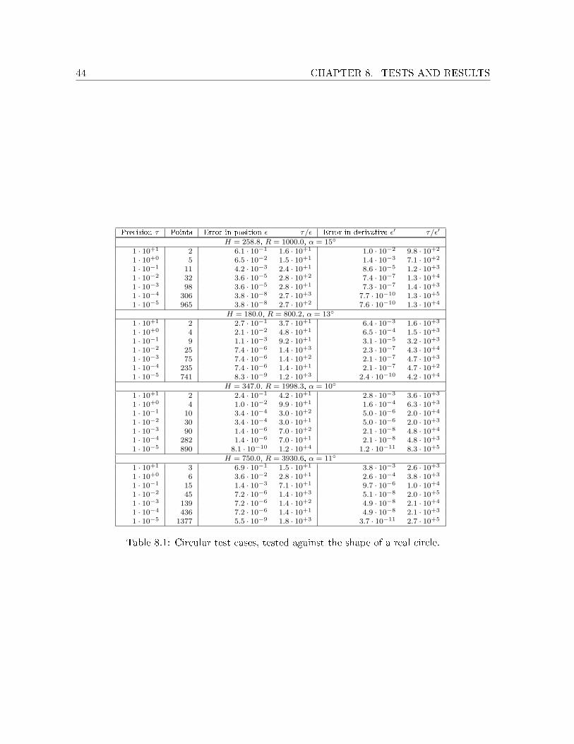
If the bottom of the shaft is exactly on the `average radius' circle, we know that it will takeon the shape of a circular arc. In table 8.1, four of these cases are tested. The �rst set ofdimensions are from a drill head Koese was designing at the time of writing; the other threeare also realistic sets of dimensions and were taken from [2].

The errors ε and ε′ were found by measuring the deviation of the computed spline fromthe real circle at 100 points, equally spaced on the z-axis. For ε, the Euclidean distance in thexy-plane was computed. For ε′ the Euclidean norm of the di�erence between the derivativeswas used.

It is immediately clear from the τ/ε column, which should be greater than 1 everywhere,that the errors ε in the result are within the speci�ed error bound τ . Looking at τ/ε′, we seethat the error ε′ in the derivative is even orders of magnitude smaller than τ .

8.2 Comparison to accurate computations

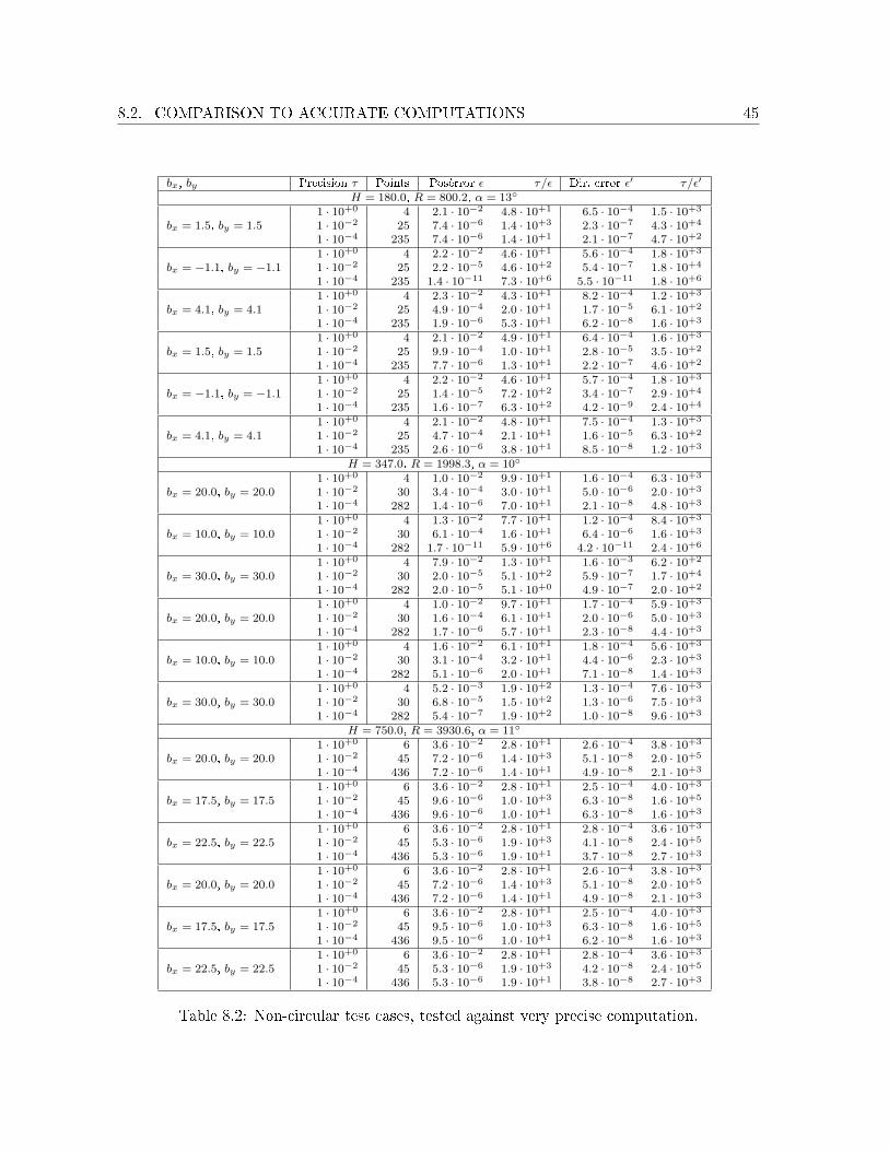
For shafts that do not assume a circular shape, we need a precise computation to compare theresults to. Table 8.2 gives some of these cases. The three examples from [2] were reused here;for brevity, the �rst example from section 8.1 is omitted. The shift with respect to the idealposition is (bx, by).

The `exact' result was acquired by setting τ = 1 · 10−6 (one nanometre). This resulted ina shaft shape consisting of 2000 to 3000 points in all cases. The errors ε and ε′ were found bymeasuring the deviation in the xy-plane at 100 points, similar to the circular cases.

We observe that these more di�cult cases do not pose a problem for the algorithm either.The error ε stays within its bound τ , and again ε′ is orders of magnitude smaller than τ .

44 CHAPTER 8. TESTS AND RESULTS

Precision τ Points Error in position ε τ/ε Error in derivative ε′ τ/ε′

H = 258.8, R = 1000.0, α = 15◦

1 · 10+1 2 6.1 · 10−1 1.6 · 10+1 1.0 · 10−2 9.8 · 10+2

1 · 10+0 5 6.5 · 10−2 1.5 · 10+1 1.4 · 10−3 7.1 · 10+2

1 · 10−1 11 4.2 · 10−3 2.4 · 10+1 8.6 · 10−5 1.2 · 10+3

1 · 10−2 32 3.6 · 10−5 2.8 · 10+2 7.4 · 10−7 1.3 · 10+4

1 · 10−3 98 3.6 · 10−5 2.8 · 10+1 7.3 · 10−7 1.4 · 10+3

1 · 10−4 306 3.8 · 10−8 2.7 · 10+3 7.7 · 10−10 1.3 · 10+5

1 · 10−5 965 3.8 · 10−8 2.7 · 10+2 7.6 · 10−10 1.3 · 10+4

H = 180.0, R = 800.2, α = 13◦

1 · 10+1 2 2.7 · 10−1 3.7 · 10+1 6.4 · 10−3 1.6 · 10+3

1 · 10+0 4 2.1 · 10−2 4.8 · 10+1 6.5 · 10−4 1.5 · 10+3

1 · 10−1 9 1.1 · 10−3 9.2 · 10+1 3.1 · 10−5 3.2 · 10+3

1 · 10−2 25 7.4 · 10−6 1.4 · 10+3 2.3 · 10−7 4.3 · 10+4

1 · 10−3 75 7.4 · 10−6 1.4 · 10+2 2.1 · 10−7 4.7 · 10+3

1 · 10−4 235 7.4 · 10−6 1.4 · 10+1 2.1 · 10−7 4.7 · 10+2

1 · 10−5 741 8.3 · 10−9 1.2 · 10+3 2.4 · 10−10 4.2 · 10+4

H = 347.0, R = 1998.3, α = 10◦

1 · 10+1 2 2.4 · 10−1 4.2 · 10+1 2.8 · 10−3 3.6 · 10+3

1 · 10+0 4 1.0 · 10−2 9.9 · 10+1 1.6 · 10−4 6.3 · 10+3

1 · 10−1 10 3.4 · 10−4 3.0 · 10+2 5.0 · 10−6 2.0 · 10+4

1 · 10−2 30 3.4 · 10−4 3.0 · 10+1 5.0 · 10−6 2.0 · 10+3

1 · 10−3 90 1.4 · 10−6 7.0 · 10+2 2.1 · 10−8 4.8 · 10+4

1 · 10−4 282 1.4 · 10−6 7.0 · 10+1 2.1 · 10−8 4.8 · 10+3

1 · 10−5 890 8.1 · 10−10 1.2 · 10+4 1.2 · 10−11 8.3 · 10+5

H = 750.0, R = 3930.6, α = 11◦

1 · 10+1 3 6.9 · 10−1 1.5 · 10+1 3.8 · 10−3 2.6 · 10+3

1 · 10+0 6 3.6 · 10−2 2.8 · 10+1 2.6 · 10−4 3.8 · 10+3

1 · 10−1 15 1.4 · 10−3 7.1 · 10+1 9.7 · 10−6 1.0 · 10+4

1 · 10−2 45 7.2 · 10−6 1.4 · 10+3 5.1 · 10−8 2.0 · 10+5

1 · 10−3 139 7.2 · 10−6 1.4 · 10+2 4.9 · 10−8 2.1 · 10+4

1 · 10−4 436 7.2 · 10−6 1.4 · 10+1 4.9 · 10−8 2.1 · 10+3

1 · 10−5 1377 5.5 · 10−9 1.8 · 10+3 3.7 · 10−11 2.7 · 10+5

Table 8.1: Circular test cases, tested against the shape of a real circle.

8.2. COMPARISON TO ACCURATE COMPUTATIONS 45

bx, by Precision τ Points Poserror ε τ/ε Dir. error ε′ τ/ε′

H = 180.0, R = 800.2, α = 13◦

bx = 1.5, by = 1.51 · 10+0 4 2.1 · 10−2 4.8 · 10+1 6.5 · 10−4 1.5 · 10+3

1 · 10−2 25 7.4 · 10−6 1.4 · 10+3 2.3 · 10−7 4.3 · 10+4

1 · 10−4 235 7.4 · 10−6 1.4 · 10+1 2.1 · 10−7 4.7 · 10+2

bx = −1.1, by = −1.11 · 10+0 4 2.2 · 10−2 4.6 · 10+1 5.6 · 10−4 1.8 · 10+3

1 · 10−2 25 2.2 · 10−5 4.6 · 10+2 5.4 · 10−7 1.8 · 10+4

1 · 10−4 235 1.4 · 10−11 7.3 · 10+6 5.5 · 10−11 1.8 · 10+6

bx = 4.1, by = 4.11 · 10+0 4 2.3 · 10−2 4.3 · 10+1 8.2 · 10−4 1.2 · 10+3

1 · 10−2 25 4.9 · 10−4 2.0 · 10+1 1.7 · 10−5 6.1 · 10+2

1 · 10−4 235 1.9 · 10−6 5.3 · 10+1 6.2 · 10−8 1.6 · 10+3

bx = 1.5, by = 1.51 · 10+0 4 2.1 · 10−2 4.9 · 10+1 6.4 · 10−4 1.6 · 10+3

1 · 10−2 25 9.9 · 10−4 1.0 · 10+1 2.8 · 10−5 3.5 · 10+2

1 · 10−4 235 7.7 · 10−6 1.3 · 10+1 2.2 · 10−7 4.6 · 10+2

bx = −1.1, by = −1.11 · 10+0 4 2.2 · 10−2 4.6 · 10+1 5.7 · 10−4 1.8 · 10+3

1 · 10−2 25 1.4 · 10−5 7.2 · 10+2 3.4 · 10−7 2.9 · 10+4

1 · 10−4 235 1.6 · 10−7 6.3 · 10+2 4.2 · 10−9 2.4 · 10+4

bx = 4.1, by = 4.11 · 10+0 4 2.1 · 10−2 4.8 · 10+1 7.5 · 10−4 1.3 · 10+3

1 · 10−2 25 4.7 · 10−4 2.1 · 10+1 1.6 · 10−5 6.3 · 10+2

1 · 10−4 235 2.6 · 10−6 3.8 · 10+1 8.5 · 10−8 1.2 · 10+3

H = 347.0, R = 1998.3, α = 10◦

bx = 20.0, by = 20.01 · 10+0 4 1.0 · 10−2 9.9 · 10+1 1.6 · 10−4 6.3 · 10+3

1 · 10−2 30 3.4 · 10−4 3.0 · 10+1 5.0 · 10−6 2.0 · 10+3

1 · 10−4 282 1.4 · 10−6 7.0 · 10+1 2.1 · 10−8 4.8 · 10+3

bx = 10.0, by = 10.01 · 10+0 4 1.3 · 10−2 7.7 · 10+1 1.2 · 10−4 8.4 · 10+3

1 · 10−2 30 6.1 · 10−4 1.6 · 10+1 6.4 · 10−6 1.6 · 10+3

1 · 10−4 282 1.7 · 10−11 5.9 · 10+6 4.2 · 10−11 2.4 · 10+6

bx = 30.0, by = 30.01 · 10+0 4 7.9 · 10−2 1.3 · 10+1 1.6 · 10−3 6.2 · 10+2

1 · 10−2 30 2.0 · 10−5 5.1 · 10+2 5.9 · 10−7 1.7 · 10+4

1 · 10−4 282 2.0 · 10−5 5.1 · 10+0 4.9 · 10−7 2.0 · 10+2

bx = 20.0, by = 20.01 · 10+0 4 1.0 · 10−2 9.7 · 10+1 1.7 · 10−4 5.9 · 10+3

1 · 10−2 30 1.6 · 10−4 6.1 · 10+1 2.0 · 10−6 5.0 · 10+3

1 · 10−4 282 1.7 · 10−6 5.7 · 10+1 2.3 · 10−8 4.4 · 10+3

bx = 10.0, by = 10.01 · 10+0 4 1.6 · 10−2 6.1 · 10+1 1.8 · 10−4 5.6 · 10+3

1 · 10−2 30 3.1 · 10−4 3.2 · 10+1 4.4 · 10−6 2.3 · 10+3

1 · 10−4 282 5.1 · 10−6 2.0 · 10+1 7.1 · 10−8 1.4 · 10+3

bx = 30.0, by = 30.01 · 10+0 4 5.2 · 10−3 1.9 · 10+2 1.3 · 10−4 7.6 · 10+3

1 · 10−2 30 6.8 · 10−5 1.5 · 10+2 1.3 · 10−6 7.5 · 10+3

1 · 10−4 282 5.4 · 10−7 1.9 · 10+2 1.0 · 10−8 9.6 · 10+3

H = 750.0, R = 3930.6, α = 11◦

bx = 20.0, by = 20.01 · 10+0 6 3.6 · 10−2 2.8 · 10+1 2.6 · 10−4 3.8 · 10+3

1 · 10−2 45 7.2 · 10−6 1.4 · 10+3 5.1 · 10−8 2.0 · 10+5

1 · 10−4 436 7.2 · 10−6 1.4 · 10+1 4.9 · 10−8 2.1 · 10+3

bx = 17.5, by = 17.51 · 10+0 6 3.6 · 10−2 2.8 · 10+1 2.5 · 10−4 4.0 · 10+3

1 · 10−2 45 9.6 · 10−6 1.0 · 10+3 6.3 · 10−8 1.6 · 10+5

1 · 10−4 436 9.6 · 10−6 1.0 · 10+1 6.3 · 10−8 1.6 · 10+3

bx = 22.5, by = 22.51 · 10+0 6 3.6 · 10−2 2.8 · 10+1 2.8 · 10−4 3.6 · 10+3

1 · 10−2 45 5.3 · 10−6 1.9 · 10+3 4.1 · 10−8 2.4 · 10+5

1 · 10−4 436 5.3 · 10−6 1.9 · 10+1 3.7 · 10−8 2.7 · 10+3

bx = 20.0, by = 20.01 · 10+0 6 3.6 · 10−2 2.8 · 10+1 2.6 · 10−4 3.8 · 10+3

1 · 10−2 45 7.2 · 10−6 1.4 · 10+3 5.1 · 10−8 2.0 · 10+5

1 · 10−4 436 7.2 · 10−6 1.4 · 10+1 4.9 · 10−8 2.1 · 10+3

bx = 17.5, by = 17.51 · 10+0 6 3.6 · 10−2 2.8 · 10+1 2.5 · 10−4 4.0 · 10+3

1 · 10−2 45 9.5 · 10−6 1.0 · 10+3 6.3 · 10−8 1.6 · 10+5

1 · 10−4 436 9.5 · 10−6 1.0 · 10+1 6.2 · 10−8 1.6 · 10+3

bx = 22.5, by = 22.51 · 10+0 6 3.6 · 10−2 2.8 · 10+1 2.8 · 10−4 3.6 · 10+3

1 · 10−2 45 5.3 · 10−6 1.9 · 10+3 4.2 · 10−8 2.4 · 10+5

1 · 10−4 436 5.3 · 10−6 1.9 · 10+1 3.8 · 10−8 2.7 · 10+3

Table 8.2: Non-circular test cases, tested against very precise computation.

46 CHAPTER 8. TESTS AND RESULTS

8.3 Real-world tests

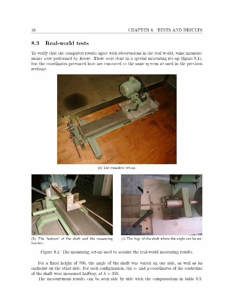
To verify that the computed results agree with observations in the real world, some measure-ments were performed by Koese. These were done in a special measuring set-up (�gure 8.1),but the coordinates presented here are converted to the same system as used in the previoussections.

(a) The complete set-up.

(b) The `bottom' of the shaft and the measuringbracket.

(c) The `top' of the shaft where the angle can be set.

Figure 8.1: The measuring set-up used to acquire the real-world measuring results.

For a �xed height of 700, the angle of the shaft was varied on one side, as well as itsendpoint on the other side. For each con�guration, the x- and y-coordinates of the centrelineof the shaft were measured halfway, at h = 350.

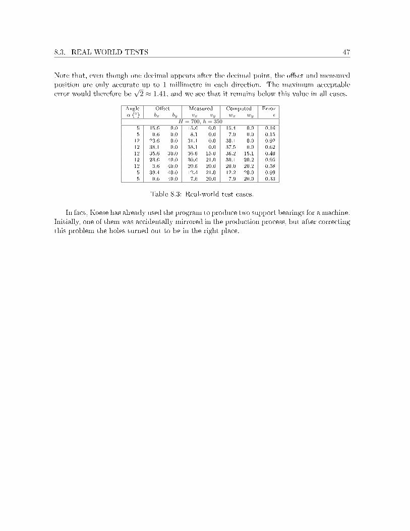
The measurement results can be seen side by side with the computations in table 8.3.

8.3. REAL-WORLD TESTS 47

Note that, even though one decimal appears after the decimal point, the o�set and measuredposition are only accurate up to 1 millimetre in each direction. The maximum acceptableerror would therefore be

√2 ≈ 1.41, and we see that it remains below this value in all cases.

Angle O�set Measured Computed Errorα (◦) bx by vx vy wx wy ε

H = 700, h = 3505 15.6 0.0 15.6 0.0 15.4 0.0 0.165 0.6 0.0 8.1 0.0 7.9 0.0 0.1512 23.6 0.0 31.1 0.0 30.1 0.0 0.9212 38.1 0.0 38.1 0.0 37.5 0.0 0.6212 35.6 30.0 36.6 15.0 36.2 15.1 0.4012 23.6 40.0 30.6 21.0 30.1 20.2 0.9512 3.6 40.0 20.6 20.0 20.0 20.2 0.585 -39.4 40.0 -12.4 21.0 -12.2 20.0 0.995 0.6 40.0 7.6 20.0 7.9 20.0 0.33

Table 8.3: Real-world test cases.

In fact, Koese has already used the program to produce two support bearings for a machine.Initially, one of them was accidentally mirrored in the production process, but after correctingthis problem the holes turned out to be in the right place.

48

49

Chapter 9

Conclusion

The bending of shafts, rods or beams is an elementary problem in mathematical physics, butis often only treated in a linearised form in two dimensions. The addition of a third dimensionand the removal of the linearisations complicate the problem.

Equations can be derived using a physical model involving the Bernoulli-Euler equation.Two parametrisations of the bending shaft have been presented, one more general and elegant,but more complex to use, the other more speci�c to this particular application and thereforeposing a problem that is easier to solve.

The resulting di�erential equations are analytically unsolvable. A shooting method is ableto produce a numerical solution. The method involves a fourth-order Runge-Kutta integrationand a Broyden multidimensional equation solver, followed by a piecewise cubic polynomialinterpolation.

It can be hard to estimate the the error in any numerical approximation, making it di�cultto keep the error within a speci�ed bound. Using assumptions that hold fairly well in practicalsituations, it has been shown that the results from the provided algorithm remain within thespeci�ed error bound in test cases derived from practical situations.

Based on a set of functional and nonfunctional requirements, a user-friendly user interfacehas been designed to access these underlying algorithms. A technical design was made tofacilitate easy maintenance of the program. The program was implemented in C#.

Unit tests have shown, to a certain degree, the correctness of the program. Moreover, theprogram has already shown its use and usability in practice.

50

51

Bibliography

[1] Koese Engineering: Multi Compact Drilling, Drilling Dotcodes, Micro-EDM and Proto-

typing . URL http://www.koese.nl/.

[2] Hartono, Sri Subarinah, Sudi Prayitno, F.P.H. van Beckum (supervisor). Curvature of

Flexible Shafts in Multiple Compact Drilling . 1996. Unpublished.

[3] Richard L. Burden, J. Douglas Faires. Numerical Analysis (Brooks/Cole, 2001), seventhed.

[4] DXF: Drawing Exchange Format . URL http://www.autodesk.com/techpubs/autocad/

acadr14/dxf/index.htm.

[5] SolidWorks � 3D Mechanical Design and 3D CAD Software. URL http://www.

solidworks.com/.

[6] The C# Language. URL http://msdn2.microsoft.com/en-us/vcsharp/aa336809.

aspx.

[7] .NET Framework Developer Center . URL http://msdn2.microsoft.com/en-us/

netframework/default.aspx.

[8] Mono. URL http://www.mono-project.com/.

[9] Windows Forms. URL http://msdn2.microsoft.com/en-us/netframework/aa497342.

aspx.

[10] Visual Studio 2005 Developer Center . URL http://msdn2.microsoft.com/en-us/

vstudio/default.aspx.

[11] NUnit . URL http://www.nunit.org/.

52

53

Appendix A

Pseudocode algorithms

A.1 The Broyden algorithm

This is the pseudocode version of Broyden's method, taken from [3, pp. 623�624] and adaptedto meet a precision requirement in terms of the absolute error instead of the step size. Theaddition consists of lines 13�15. These replace a check on the magnitude of s after line 22.

The algorithm attempts to �nd an approximate solution to F (x) = 0, where F : Rn → Rn.

Input: function F , initial estimate x, tolerance ε, maximum number of iterations NOutput: approximate solution x

A0 := J(x) { J(x) denotes the Jacobian of F in x }5 v := F (x)

A := A−10 { matrix inverse }

s := −Avx := x + sk := 2

10 while k ≤ N do

w := vv := F (x)if ‖v‖ ≤ ε then

return x15 end if

y := v − wz := −Ay

p := −s>z { > denotes transposition }

u> := s>A

20 A := a + 1p (s + z)u>

s := −Avx := x + sk := k + 1

end while

25 fail { maximum number of iterations exceeded }