Embed Size (px)
Citation preview
Numer. Math. (2015) 129:181–209DOI 10.1007/s00211-014-0635-z
NumerischeMathematik
Computing the common zeros of two bivariate functionsvia Bézout resultants
Yuji Nakatsukasa · Vanni Noferini ·Alex Townsend
Received: 19 May 2013 / Revised: 5 March 2014 / Published online: 9 May 2014© Springer-Verlag Berlin Heidelberg 2014
Abstract The common zeros of two bivariate functions can be computed by findingthe common zeros of their polynomial interpolants expressed in a tensor Chebyshevbasis. From here we develop a bivariate rootfinding algorithm based on the hiddenvariable resultant method and Bézout matrices with polynomial entries. Using tech-niques including domain subdivision, Bézoutian regularization, and local refinementwe are able to reliably and accurately compute the simple common zeros of two smoothfunctions with polynomial interpolants of very high degree (≥1,000). We analyze theresultant method and its conditioning by noting that the Bézout matrices are matrixpolynomials. Two implementations are available: one on the Matlab Central FileExchange and another in the roots command in Chebfun2 that is adapted to suitChebfun’s methodology.
Mathematics Subject Classification (2000) 65D15 · 65F15 · 65F22
Yuji Nakatsukasa was partially supported by EPSRC grant EP/I005293/1.Vanni Noferini was supported by ERC Advanced Grant MATFUN (267526).Alex Townsend was supported by EPSRC grant EP/P505666/1 and the ERC grant FP7/2007-2013 toL. N. Trefethen.
Y. NakatsukasaDepartment of Mathematical Informatics, Graduate School of Information Science and Technology,University of Tokyo, Tokyo 113-8656, Japane-mail: [email protected]
V. Noferini (B)School of Mathematics, University of Manchester, Manchester M13 9PL, UKe-mail: [email protected]
A. TownsendMathematical Institute, University of Oxford, Oxford OX2 6GG, UKe-mail: [email protected]
123
182 Y. Nakatsukasa et al.
1 Introduction
There are two operations on bivariate functions that are commonly referred to asrootfinding: (1) Finding the zero level curves of f (x, y), and (2) Finding the commonzeros of f (x, y) and g(x, y). Despite sharing the same name these operations aremathematically distinct; the first has solutions along curves while the second, typically,has isolated solutions. In this paper we concentrate on the second, that is, computingall the real pairs (x, y) ∈ [−1, 1] × [−1, 1] such that
(f (x, y)
g(x, y)
)= 0 (1)
under the assumption that f and g are real-valued in [−1, 1]×[−1, 1] and the solutionset is zero-dimensional, i.e., the solutions are isolated. In this typical situation wedescribe a robust, accurate, and fast numerical algorithm that can solve problems ofmuch higher degree than in previous studies.
Our first step is to replace f and g in (1) by polynomial interpolants p and q,respectively, before finding the common zeros of the corresponding polynomial sys-tem. Throughout this paper we assume that f and g are smooth bivariate functions,and p and q are their polynomial interpolants, which approximate f and g to relativemachine precision. The polynomials p and q are of the form:
p(x, y) =m p∑i=0
n p∑j=0
Pi j Ti (y)Tj (x), q(x, y) =mq∑i=0
nq∑j=0
Qi j Ti (y)Tj (x), (2)
where Tj (x) = cos( j cos−1(x)) is the Chebyshev polynomial of degree j , and P ∈R
(m p+1)×(n p+1), Q ∈ R(mq+1)×(nq+1) are the matrices of coefficients. The polynomial
interpolants p and q satisfy
‖ f − p‖∞ = O(u)‖ f ‖∞, ‖g − q‖∞ = O(u)‖g‖∞, (3)
where ‖ f ‖∞ = maxx,y∈[−1,1] | f (x, y)| and u is the unit roundoff.The resulting polynomial system, p(x, y) = q(x, y) = 0, is solved by an algorithm
based on the hidden variable resultant method and Bézout resultant matrices thathave entries containing univariate polynomials. One component of the solutions iscomputed by solving a polynomial eigenvalue problem via a standard approach inthe matrix polynomial literature known as linearization [22] and a robust eigenvaluesolver, such as the eig command in Matlab. The remaining component is found byunivariate rootfinding based on the colleague matrix [13]. Usually, resultant methodshave several computational drawbacks and our algorithm is motivated by attemptingto overcome them:
1. Computational complexity: The complexity of resultant methods based on Bézout(and Sylvester) matrices grows like the degree of p and q to the power of 6.Therefore, computations quickly become unfeasible when the degrees are largerthan, say, 30, and this is one reason why the literature concentrates on examples
123
Computing common zeros of two bivariate functions 183
with degree 20, or smaller [1,10,19,28,34]. Typically, we reduce the complexity toquartic scaling, and sometimes even further, by using domain subdivision, whichis beneficial for both accuracy and efficiency (see Sect. 4). Subdivision can allowus to compute the common zeros to (1) with polynomial interpolants of degree aslarge as 1,000, or more.
2. Conditioning: We analyze the conditioning of Bézout matrix polynomials andderive condition numbers. The analysis reveals that recasting the problem in termsof resultants can worsen the conditioning of the problem, and we resolve thisvia a local refinement process. The Bézout local refinement process improves theaccuracy significantly, and also identifies and removes spurious zeros; a well-known difficulty for resultant-based methods.
3. Numerical instability: The Bézout matrix polynomial is often numerically closeto singular, leading to numerical difficulties, and to overcome this we apply a reg-ularization step. The regularization we employ crucially depends on the symmetryof Bézout matrices. We proceed to solve the polynomial eigenvalue problem bylinearization, which avoids the interpolation of highly oscillatory determinants ofresultants, overcoming further numerical difficulties.
4. Robustness: It is not essential for a bivariate rootfinding method to construct aneigenvalue problem, but if it does it is convenient and can improve robustness.For this reason we solve an eigenvalue problem to find one component of thesolutions to p(x, y) = q(x, y) = 0, and a second eigenvalue problem to findthe other. Therefore, our algorithm inherits some of its robustness from the QZalgorithm [23], which is implemented in the eig command in Matlab.
5. Resultant construction: Resultant methods are more commonly based on Sylvesterresultant matrices that are preferred due to their ease of construction, and this isespecially true when dealing with polynomials expressed in an orthogonal polyno-mial basis rather than the monomial basis. However, the Bézout resultant matrices,when using the tensor Chebyshev basis, are also easily constructed by using theMatlab code in [39]. We choose Bézout over Sylvester because its conditioningcan be analyzed (see Sect. 5) so its numerical behavior is better understood, andits symmetry can be exploited.
For definiteness, unless stated otherwise, we consider the problem of finding the com-mon zeros in the domain [−1, 1]× [−1, 1], but the algorithm and codes deal with anyrectangular domain.
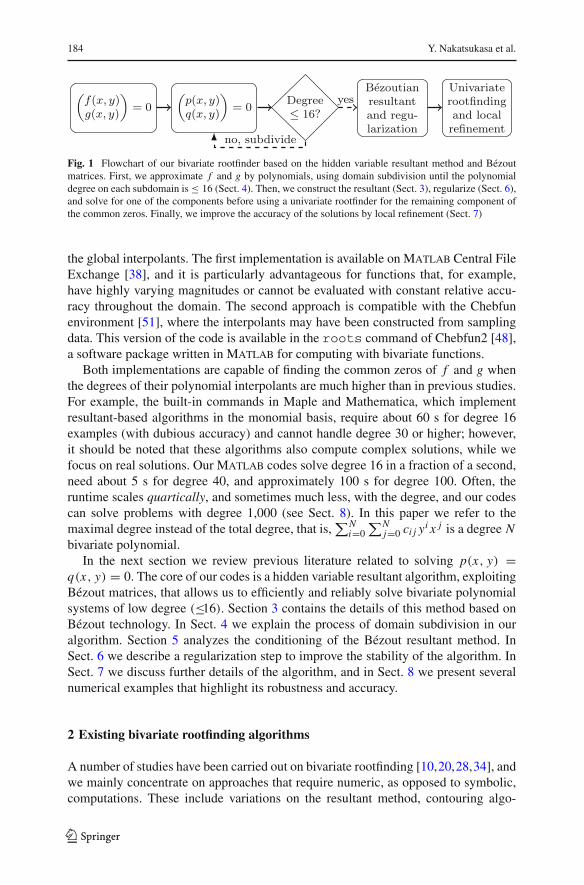
Figure 1 summarizes the main steps in our bivariate rootfinding algorithm basedon the hidden variable resultant method, domain subdivision, Bézout regularization,and the tensor Chebyshev basis. In particular, it is crucial that we express the polyno-mial interpolants of f and g in a tensor Chebyshev basis so that we can employ fasttransforms for interpolation based on the fast Fourier transform, overcome numericalinstability associated with interpolation at equally-spaced points, and prevent the com-mon zeros from being sensitive to perturbations of the polynomial coefficients [52].
Subdivision is also a key part of our algorithm and is crucial for the method tobe practical for polynomial systems of high degree. There are two alternative subdi-vision strategies. The first consists of resampling the original functions f and g toconstruct new interpolants on each subdomain and the second involves resampling
123
184 Y. Nakatsukasa et al.
Fig. 1 Flowchart of our bivariate rootfinder based on the hidden variable resultant method and Bézoutmatrices. First, we approximate f and g by polynomials, using domain subdivision until the polynomialdegree on each subdomain is≤ 16 (Sect. 4). Then, we construct the resultant (Sect. 3), regularize (Sect. 6),and solve for one of the components before using a univariate rootfinder for the remaining component ofthe common zeros. Finally, we improve the accuracy of the solutions by local refinement (Sect. 7)
the global interpolants. The first implementation is available on Matlab Central FileExchange [38], and it is particularly advantageous for functions that, for example,have highly varying magnitudes or cannot be evaluated with constant relative accu-racy throughout the domain. The second approach is compatible with the Chebfunenvironment [51], where the interpolants may have been constructed from samplingdata. This version of the code is available in the roots command of Chebfun2 [48],a software package written in Matlab for computing with bivariate functions.
Both implementations are capable of finding the common zeros of f and g whenthe degrees of their polynomial interpolants are much higher than in previous studies.For example, the built-in commands in Maple and Mathematica, which implementresultant-based algorithms in the monomial basis, require about 60 s for degree 16examples (with dubious accuracy) and cannot handle degree 30 or higher; however,it should be noted that these algorithms also compute complex solutions, while wefocus on real solutions. Our Matlab codes solve degree 16 in a fraction of a second,need about 5 s for degree 40, and approximately 100 s for degree 100. Often, theruntime scales quartically, and sometimes much less, with the degree, and our codescan solve problems with degree 1,000 (see Sect. 8). In this paper we refer to themaximal degree instead of the total degree, that is,
∑Ni=0
∑Nj=0 ci j yi x j is a degree N
bivariate polynomial.In the next section we review previous literature related to solving p(x, y) =
q(x, y) = 0. The core of our codes is a hidden variable resultant algorithm, exploitingBézout matrices, that allows us to efficiently and reliably solve bivariate polynomialsystems of low degree (≤16). Section 3 contains the details of this method based onBézout technology. In Sect. 4 we explain the process of domain subdivision in ouralgorithm. Section 5 analyzes the conditioning of the Bézout resultant method. InSect. 6 we describe a regularization step to improve the stability of the algorithm. InSect. 7 we discuss further details of the algorithm, and in Sect. 8 we present severalnumerical examples that highlight its robustness and accuracy.
2 Existing bivariate rootfinding algorithms
A number of studies have been carried out on bivariate rootfinding [10,20,28,34], andwe mainly concentrate on approaches that require numeric, as opposed to symbolic,computations. These include variations on the resultant method, contouring algo-
123
Computing common zeros of two bivariate functions 185
rithms, homotopy continuation, and a two-parameter eigenvalue approach. It is alsoworth mentioning the existence of important approaches based on Gröbner bases, eventhough some symbolic manipulations are usually employed [17]. Generally, Gröbnerbases are feasible only for small degree polynomial systems because of their com-plexity and numerical instability.
2.1 Resultant methods
The hidden variable resultant method is based on selecting one variable, say y, andwriting p and q as polynomials in x with coefficients in R[y], that is,
p(x, y) = py(x) =n p∑j=0
α j (y)x j , q(x, y) = qy(x) =nq∑j=0
β j (y)x j . (4)
Note that, although we have expressed (4) in the monomial basis, any polynomial basiscan be used, see, for example, [9]. Monomials are the standard basis in the literature[18,21], due to their simplicity and flexibility for algebraic manipulations. On theother hand, the Chebyshev polynomial basis is a better choice for numerical stabilityon the real interval [−1, 1] [50]. For this reason, we always express polynomials inthe Chebyshev basis.
The two polynomials py(x) and qy(x) in (4), thought of as univariate in x , have acommon zero if and only if a resultant matrix is singular [5]. Therefore, the y-valuesof the solutions to (1) can be computed by finding the y-values such that a resultantmatrix is singular.
There are many different resultant matrices such as Sylvester [18], Bézout [8],and other matrices [5,21,29], and this choice can affect subsequent efficiency (seeTable 1) and conditioning (see Sect. 5). Usually, resultant matrices are constructedfrom polynomials expressed in the monomial basis [10,34], but they can be derivedwhen using any other bases [9].
Finding the y-values such that the resultant matrix is singular is equivalent to apolynomial eigenvalue problem, and many techniques exist such as methods basedon contour integrals [2,7], Newton-type methods, inverse iteration methods (see thereview [36]), the Ehrlich–Aberth method [11], and the standard approach of solvingvia linearization [22]. In our implementation we use linearization, which replacesa polynomial eigenvalue problem with a generalized eigenvalue problem with thesame eigenvalues and Jordan structure [22]. Then we apply the QZ algorithm to thelinearization; for a discussion of possible alternatives, see [36]. We leave for futureresearch the study of the possible incorporation in our algorithm of alternative matrixpolynomial eigensolvers.
Another related approach is the u-resultant method, which works similarly andstarts by introducing a dummy variable to make the polynomial interpolants homo-geneous. The hidden variable resultant method is then applied to the new polynomialsystem selecting the dummy variable first. This is quite natural because it ensuresthat the x- and y-variables are treated in the same way, but unfortunately, making a
123
186 Y. Nakatsukasa et al.
polynomial homogeneous inherently requires the monomial basis, and hence, entailsa corresponding numerical instability.
Some resultant methods first apply a coordinate rotation, such as theBivariateRootfinding command in Maple, which is used to ensure that twocommon zeros do not share the same y-value. We provide a careful case-by-casestudy to show that our approach does not require such a transform. Furthermore, otherchanges of variables can be applied, such as x = (z+ω)/2 and y = (z−ω)/2 [45], thenselecting the variable ω, which satisfies ω = z when x and y are real. We have foundthat such changes of variables give little improvement for most practical examples.
2.2 Contouring algorithms
Contouring algorithms such as marching squares and marching triangles [26] areemployed in computer graphics to generate zero level curves of bivariate functions.These contouring algorithms can be very efficient at solving (1), and until this paperthe roots(f,g) command in Chebfun2 exclusively employed such a contouringapproach [48]. In the older version of Chebfun2 the zero level curves of f and gwere computed separately using the Matlab command contourc, and then theintersections of these zero level curves were used as initial guesses for Newton’siteration.
Contouring algorithms suffer from several drawbacks:
1. The level curves of f and g may not be smooth even for very low degree polyno-mials, for example, f (x, y) = y2 − x3.
2. The number of disconnected components of the level curves of f and g can bepotentially quite large [24].
3. Contours of f or g are not always grouped correctly, leading to the potential formissed solutions.
4. The zero level curves must be discretized and therefore, the algorithm requires afine tuning of parameters to balance efficiency and reliability.
For many practical applications solving (1) via a contouring algorithm may be anadequate approach, but not always.
Remark 1 The roots(f,g) command in Chebfun2 implements both the algorithmbased on a contouring algorithm and the approach described in this paper. An optionalparameter can be supplied to select one or the other of these choices. We have decidedto keep the contouring approach as an option because it can sometimes run faster, butwe treat its computed solutions with suspicion, and we employ the algorithm in thispaper as a robust alternative.
2.3 Other numerical methods
Homotopy continuation methods [44] have a simple underlying approach based onsolving an initial easy polynomial system that can be continuously deformed into (1).Along the way several polynomial systems are solved with the current solution set
123
Computing common zeros of two bivariate functions 187
being used as an initial guess for the next. These methods have received significantresearch attention and are a purely numerical approach that can solve multivariaterootfinding problems [6,44].
The two-parameter eigenvalue approach constructs a determinantal expression forthe polynomial interpolants to f and g and then rewrites p(x, y) = q(x, y) = 0 as atwo-parameter eigenvalue problem [3],
A1v = x B1v + yC1v, A2w = x B2w + yC2w.
This approach has advantages because the two-parameter eigenvalue problem can besolved with the QZ algorithm [27], or other techniques [27]. However, the constructionof a determinantal expression, and hence the matrices Ai , Bi , Ci for i = 1, 2, currentlyrequires the solution of a multivariate polynomial system [41]. Alternatively, matricesof much larger size can be constructed using a generalized companion form, but theseare too large to be efficient [37].
3 The resultant method with Bézout matrices
We now describe the hidden variable resultant method using Bézout matrices thatforms the core of our algorithm. The initial step of the resultant method selects avariable to solve for first, and our choice is based on the efficiency of subsequentsteps. For simplicity, throughout the paper, we select the y-variable and write thepolynomials p(x, y) and q(x, y) as functions of x with coefficients in R[y], using theChebyshev basis:
py(x) =n p∑j=0
α j (y)Tj (x), qy(x) =nq∑j=0
β j (y)Tj (x), x ∈ [−1, 1], (5)
where α j , β j ∈ R[y], i.e., polynomials in y with real coefficients,have the polynomialexpansions
α j (y) =m p∑i=0
Pi j Ti (y), β j (y) =mq∑i=0
Qi j Ti (y), y ∈ [−1, 1],
where the matrices P and Q are as in (2).The (Chebyshev) Bézout matrix of py and qy in (5), denoted by B(py, qy), is
defined1 by B(py, qy) = (bi j )0≤i, j≤N−1 [39], where N = max(n p, nq) and theentries satisfy
py(s)qy(t)− py(t)qy(s)
s − t=
N−1∑i, j=0
bi j Ti (s)Tj (t). (6)
1 Historically, this functional viewpoint of a Bézout matrix is in fact due to Cayley, who modified theoriginal method of Bézout, both in the monomial basis [43, Lesson IX].
123
188 Y. Nakatsukasa et al.
We observe that since bi j ∈ R[y], B(py, qy) can be expressed as a matrix polyno-mial [22], i.e., a polynomial with matrix coefficients, that is
B(y) = B(py, qy)(y) =M∑
i=0
Ai Ti (y), Ai ∈ RN×N , (7)
where M = m p+mq is the sum of the degrees of p(x, y) and q(x, y) in the y-variable.The resultant of py and qy is defined as the determinant of B(y), which is a scalarunivariate polynomial in y. The usual resultant definition is via the Sylvester matrix,but we use the symmetric Bézout matrix, and later explain that these two definitionsare subtly different (see Sect. 3.1).
It is well-known [18, Proposition 3.5.8 and Corollary 3.5.4] that two bivariatepolynomials share a common factor in R[x, y] only if their resultant is identically zero.Throughout this paper we are assuming the solution set to (1) is zero-dimensional andhence that the polynomial interpolants p and q do not share a common factor. Thishas two important implications:
– (Bézout’s Theorem) The number of solutions to p(x, y) = q(x, y) = 0 isfinite [30, Ch. 3];
– (Non-degeneracy) The resultant, det(B(y)), is not identically zero and therefore,B(y) is a regular matrix polynomial [22].
Since the resultant is not identically zero, the solutions to
det (B(y)) = det(B(py, qy)
) = 0 (8)
are the finite eigenvalues of B(y), and we observe that if y∗ is a finite eigenvalue ofB(y), then the resultant of py∗(x) = p(x, y∗) and qy∗(x) = q(x, y∗) is zero. Usually,a zero resultant means that p(x, y∗) and q(x, y∗) share a finite common root [5], butthey can also have a “common root at infinity” (see Sect. 3.1).
The eigenvalues of B(y) can be found via linearization of matrix polynomialsexpressed in polynomial bases [33,39], which constructs a generalized eigenvalueproblem Cv = λEv with the same eigenvalues as B(y). In our implementationwe choose the colleague linearization, which is a companion-like matrix pencil for(matrix) polynomials expressed in the Chebyshev basis and employ the eig commandin Matlab to solve Cv = λEv. The process of linearization converts the problem offinding the eigenvalues of B(y), a matrix polynomial of degree M and size N , to anM N × M N generalized eigenvalue problem. Typically, the majority of the computa-tional cost of our algorithm is in solving these generalized eigenvalue problems.
After filtering out the y-values that do not correspond to solutions in [−1, 1] ×[−1, 1], the x-values are computed via two independent univariate rootfinding prob-lems: py(x) = 0 and qy(x) = 0. These univariate problems are solved by a rootfinderbased on the colleague matrix [13,51] (see Sect. 7).
The resultant method with Bézout matrices also works if we select the x-value tosolve for first, and this choice can change the cost of the computation. Let n p andm p be the degrees of p(x, y) in the x- and y-variable, respectively, and similarly
123
Computing common zeros of two bivariate functions 189
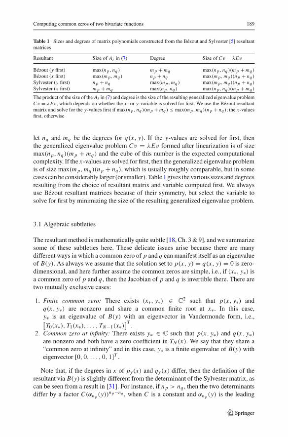
Table 1 Sizes and degrees of matrix polynomials constructed from the Bézout and Sylvester [5] resultantmatrices
Resultant Size of Ai in (7) Degree Size of Cv = λEv
Bézout (y first) max(n p, nq ) m p + mq max(n p, nq )(m p + mq )
Bézout (x first) max(m p, mq ) n p + nq max(m p, mq )(n p + nq )
Sylvester (y first) n p + nq max(m p, mq ) max(m p, mq )(n p + nq )
Sylvester (x first) m p + mq max(n p, nq ) max(n p, nq )(m p + mq )
The product of the size of the Ai in (7) and degree is the size of the resulting generalized eigenvalue problemCv = λEv, which depends on whether the x- or y-variable is solved for first. We use the Bézout resultantmatrix and solve for the y-values first if max(n p, nq )(m p +mq ) ≤ max(m p, mq )(n p + nq ); the x-valuesfirst, otherwise
let nq and mq be the degrees for q(x, y). If the y-values are solved for first, thenthe generalized eigenvalue problem Cv = λEv formed after linearization is of sizemax(n p, nq)(m p + mq) and the cube of this number is the expected computationalcomplexity. If the x-values are solved for first, then the generalized eigenvalue problemis of size max(m p, mq)(n p + nq), which is usually roughly comparable, but in somecases can be considerably larger (or smaller). Table 1 gives the various sizes and degreesresulting from the choice of resultant matrix and variable computed first. We alwaysuse Bézout resultant matrices because of their symmetry, but select the variable tosolve for first by minimizing the size of the resulting generalized eigenvalue problem.
3.1 Algebraic subtleties
The resultant method is mathematically quite subtle [18, Ch. 3 & 9], and we summarizesome of these subtleties here. These delicate issues arise because there are manydifferent ways in which a common zero of p and q can manifest itself as an eigenvalueof B(y). As always we assume that the solution set to p(x, y) = q(x, y) = 0 is zero-dimensional, and here further assume the common zeros are simple, i.e., if (x∗, y∗) isa common zero of p and q, then the Jacobian of p and q is invertible there. There aretwo mutually exclusive cases:
1. Finite common zero: There exists (x∗, y∗) ∈ C2 such that p(x, y∗) and
q(x, y∗) are nonzero and share a common finite root at x∗. In this case,y∗ is an eigenvalue of B(y) with an eigenvector in Vandermonde form, i.e.,[T0(x∗), T1(x∗), . . . , TN−1(x∗)
]T .2. Common zero at infinity: There exists y∗ ∈ C such that p(x, y∗) and q(x, y∗)
are nonzero and both have a zero coefficient in TN (x). We say that they share a“common zero at infinity” and in this case, y∗ is a finite eigenvalue of B(y) witheigenvector [0, 0, . . . , 0, 1]T .
Note that, if the degrees in x of py(x) and qy(x) differ, then the definition of theresultant via B(y) is slightly different from the determinant of the Sylvester matrix, ascan be seen from a result in [31]. For instance, if n p > nq , then the two determinantsdiffer by a factor C(αn p (y))n p−nq , when C is a constant and αn p (y) is the leading
123
190 Y. Nakatsukasa et al.
coefficient of py(x), but this does not alter the eigenvalues corresponding to finitecommon zeros.
The algebraic subtlety continues when there are many common zeros (possiblyincluding “zeros at infinity”) of p and q sharing the same y-value. In this case B(y)
has an eigenvalue with multiplicity greater than 1 even though p and q only havesimple common zeros. Furthermore, there can exist y∗ ∈ C such that either p(x, y∗) orq(x, y∗) is identically zero, in which case y∗ is an eigenvalue of B(y) with B(y∗) = 0,a zero matrix.
Eigenvalues of B(y) of multiplicity > 1 can be ill-conditioned and hence, difficult tocompute accurately, particularly in the presence of nontrivial Jordan chains. However,in the generic case where all the common zeros of p and q are simple,2 the x-values forany two common zeros with the same y-value are distinct. Moreover, the eigenvalues ofB(y) have the same geometric and algebraic multiplicity with eigenvectors spanned byVandermonde vectors span{[T0(xi ), . . . , TN−1(xi )
]T }, where xi are the x-values of thecommon zeros (xi , y∗). This means the eigenvalues of B(y) in [−1, 1] are semisimple,and hence can be obtained accurately. The intuitive explanation is that such solutionsresult only in nondefective (or semisimple) eigenvalues of B(y), and nondefectivemultiple eigenvalues are no more sensitive to perturbation than simple eigenvalues forboth matrices [46] and matrix pencils [53], showing they are well-conditioned. Thisis often overlooked and multiple eigenvalues are sometimes unnecessarily assumedto be ill-conditioned. Therefore, if the original problem (1) only has simple commonzeros, then the resultant method can compute accurate solutions and there is no needto perform a change of variables so that well-separated common zeros have differenty-values.
In the presence of multiple or near-multiple common zeros the situation becomesmore delicate, and in such cases the corresponding eigenvalues of B(y) are ill-conditioned (see Theorem 1). Our focus is on the generic case where the solutions aresimple, and a reasonable requirement for a numerical algorithm is that it detects simplecommon zeros that are not too ill-conditioned, while multiple zeros are inherently ill-conditioned and difficult to compute accurately. Our code typically computes commonzeros of multiplicity two with O(u1/2) accuracy, i.e., the error expected from a back-ward stable algorithm. However, since near-multiple solutions are also ill-conditionedany numerical scheme, including our own, suffer from inevitable numerical difficul-ties.
4 Subdivision of the domain
The Bézout resultant method of Sect. 3 requires three main features to become practi-cal: subdivision, local Bézout refinement, and regularization. The first of these is a 2Dversion of Boyd’s subdivision technique for univariate rootfinding [14,15], as utilizedfor many years in Chebfun [13,51].
2 This includes those at infinity. The requirement can be formalized, but the algebraic details are beyondthe scope of this paper.
123
Computing common zeros of two bivariate functions 191
−1 −0.5 0 0.5 1−1
−0.5
0
0.5
1
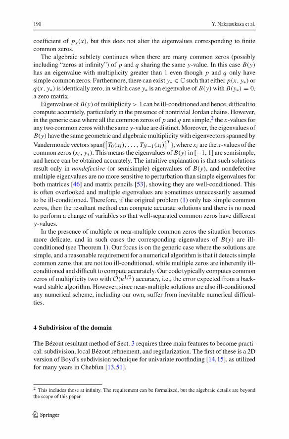
Fig. 2 Le f t Subdivision of [−1, 1]× [−1, 1] used for f = sin((x−1/10)y) cos(1/(x+ (y−9/10)+5))
and g = (y−1/10) cos((x+ (y+9/10)2/4)). The blue and red lines represent subdivisions used to ensurethe piecewise interpolants to f and g have degree ≤ 16, and the green lines are for both. The black dot isthe only common zero. Right Zero contours (blue, red) and solutions (black) for oscillatory functions fand g as in (9)
We recursively subdivide [−1, 1]×[−1, 1], in the x- and y-variable independently,until the polynomial interpolants of f and g on each subdomain are of degree ≤16, a parameter determined by experimentation. Specifically, we subdivide in x ifmax(n p, nq) > 16, and subdivide in y if max(m p, mq) > 16. Figure 2 (left) showshow [−1, 1]×[−1, 1] is subdivided for sin((x−1/10)y) cos(1/(x+(y−9/10)+5)) =(y − 1/10) cos((x + (y + 9/10)2/4)) = 0. A polynomial system of degree ≤ 16 issolved on each subdomain.
Occasionally, f and g require a different amount of subdivision in one or both ofthe coordinate directions. Regardless, we need to subdivide f and g on the same grids.For example, consider the following problem:
(f (x, y)
g(x, y)
)=
(sin(30x − y/30)+ ysin(x/30− 30y)− x
)= 0, (x, y) ∈ [−1, 1] × [−1, 1]. (9)
Here, the global interpolants p and q have polynomial degrees (m p, n p, mq , nq) =(7, 63, 62, 6), so f requires many subdivisions in x , and g requires many in y. How-ever, since f and g must be subdivided on the same grids we actually subdivide fand g many times in both coordinate directions. Figure 2 shows the zero contours andcommon zeros for (9).
We do not exactly bisect in the x- or y-direction, but instead subdivide asymmetri-cally to avoid splitting exactly at a solution to f (x, y) = g(x, y) = 0. That is, in thex-direction we subdivide [−1, 1]×[−1, 1] into the two subdomains [−1, rx ]×[−1, 1]and [rx , 1] × [−1, 1], and in the y-direction [−1, 1] × [−1, ry] and [−1, 1] × [ry, 1],where rx and ry are small arbitrary constants.3 This is to avoid accidentally subdivid-
3 We use rx ≈ −0.004 and ry ≈ −0.0005. There is no special significance of these constants apart fromthat they are small and arbitrary.
123
192 Y. Nakatsukasa et al.
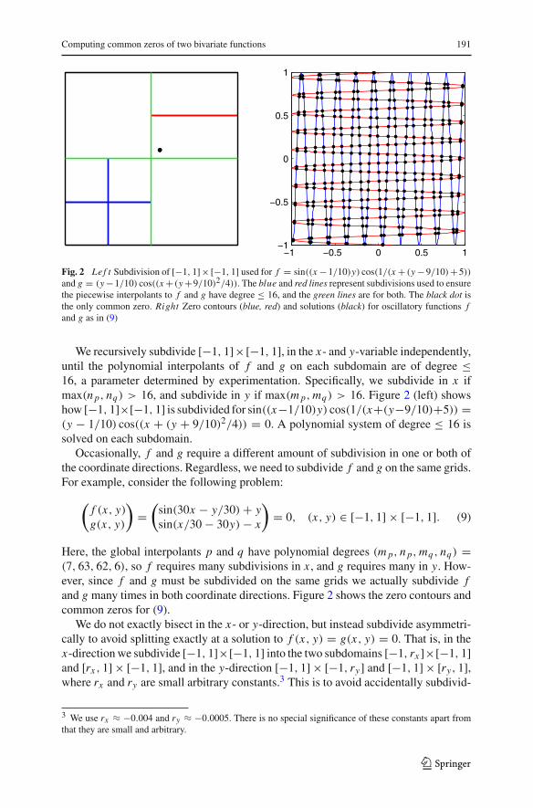
Fig. 3 Subdivision complexityis O (
nα), where
α = − log 4/ log τ and0 < τ ≤ 1 measures thereduction in polynomial degreeafter subdivision. When τ < 1/2polynomial evaluation is thedominating computational cost
0 0.2 0.4 0.6 0.80
1
2
3
4
5
6
7
τ
α
ing at a solution since problems arising in practice often have zeros at special pointslike (0, 0). Usually, a piecewise polynomial interpolant can be of lower degree than aglobal polynomial approximation, but not always. For subdivision to be computation-ally worthwhile we require that, on average, each subdivision reduces the polynomialdegree (in the x or y direction) by at least 79 %. The estimate 79 % is derived fromthe fact that 2(.79)3 ≈ 1, and each subdivision in the x-direction splits a problem intotwo, and the complexity of the algorithm depends cubically on the degree in x . Letn = max(m p, n p, mq , nq) be the maximal degree of p and q, and let d = 16 be theterminating degree for subdivsion. We define K to be the smallest integer such thatn(.79)K ≤ d, and we stop subdividing when either the degree is < d, or subdivisionhas been performed K times. After each subdivision we eliminate subdomains with2|P00| > ∑
i, j |Pi j | or 2|Q00| > ∑i, j |Qi j |, which certainly do not contain a solution.
Suppose for the moment that all the degrees of p and q are equal to n in bothx and y and that each subdivision leads to a reduction in the degree by a factor0 < τ ≤ 1. Subdividing is done k times in both x and y until nτ k ≤ d = 16, sok ≈ (log d − log n)/ log τ and we have at most 4k subdomains, each requiring O(d6)
operations to solve the local polynomial system. Therefore, the overall complexity is
O(
4k)= O
(4
log d−log nlog τ
)= O
(4−
log nlog τ
)= O
(n−
log 4log τ
).
Figure 3 shows the exponent − log 4/ log τ as a function of τ . When τ � 0.5,the overall complexity is as low as O(n2) and dominated by the cost of subdivision.When τ ≈ 0.79 the complexity is as high as O(n6), the same as without subdivision,but as long as τ < 1 subdivision is useful as it reduces the storage cost from O(n4),for storing the linearization matrix pencil, to O(n2) for storing the matrix of functionsamples.
The average degree reduction τ can take any value between 0 and 1 as the followingexamples show:
123
Computing common zeros of two bivariate functions 193
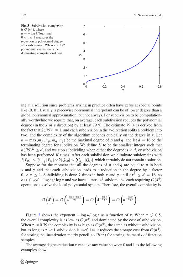
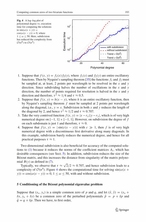
Fig. 4 A log–log plot ofpolynomial degree vs. executiontime for computing the solutionsto sin(ω(x + y)) =cos(ω(x − y)) = 0, where1 ≤ ω ≤ 50. Here, subdivisionhas reduced the complexity fromO(n6) to O(n4)
20 40 8010
−1
100
101
102
Polynomial degreeE
xecu
tion
time
with subdivisionwithout subdivision
Trend = O(n4)
Trend = O(n6)
1. Suppose that f (x, y) = f1(x) f2(y), where f1(x) and f2(y) are entire oscillatoryfunctions. Then by Nyquist’s sampling theorem [35] the functions f1 and f2 mustbe sampled at, at least, 2 points per wavelength to be resolved in the x and ydirection. Since subdividing halves the number of oscillations in the x and ydirection, the number of points required for resolution is halved in the x and ydirection and therefore, τ 2 ≈ 1/4 and τ ≈ 0.5.
2. Suppose that f (x, y) = h(x − y), where h is an entire oscillatory function, thenby Nyquist’s sampling theorem f must be sampled at 2 points per wavelengthalong the diagonal, i.e., y = x . Subdivision in both x and y reduces the length ofthe diagonal by 2, and hence τ 2 ≈ 1/2 and τ ≈ 0.707.
3. Take the very contrived function f (x, y) = |x − rx ||y− ry |, which is of very highnumerical degree on [−1, 1] × [−1, 1]. However, on subdivision the degree of fon each subdomain is just 1 and therefore, τ ≈ 0.
4. Suppose that f (x, y) = | sin(c(x − y))| with c 1, then f is of very highnumerical degree with a discontinuous first derivative along many diagonals. Inthis example, subdivision barely reduces the numerical degree, and hence for allpractical purposes τ ≈ 1.
Two-dimensional subdivision is also beneficial for accuracy of the computed solu-tions to (1) because it reduces the norms of the coefficient matrices Ai , which hasdesirable consequences (see Sect. 5). In addition, subdivision reduces the size of theBézout matrix, and this increases the distance from singularity of the matrix polyno-mial B(y) as defined in (7).
Typically, we observe that τ ≈ √2/2 ≈ 0.707, and hence subdivision leads to acomplexity of O(n4). Figure 4 shows the computational time for solving sin(ω(x +y)) = cos(ω(x − y)) = 0, 1 ≤ ω ≤ 50, with and without subdivision.
5 Conditioning of the Bézout polynomial eigenvalue problem
Suppose that (x∗, y∗) is a simple common zero of p and q, and let (x, y) = (x∗ +δx, y∗ + δy) be a common zero of the perturbed polynomials p = p + δp andq = q + δp. Then we have, to first order,
123
194 Y. Nakatsukasa et al.
0 =[
p(x, y)
q(x, y)
]=
[∂x p(x∗, y∗) ∂y p(x∗, y∗)∂x q(x∗, y∗) ∂yq(x∗, y∗)
] [δxδy
]+
[δp(x, y)
δq(x, y)
]. (10)
Our implementation initially scales p and q so that ‖p‖∞ = ‖q‖∞ = 1, where‖p‖∞ = maxx,y∈[−1,1] |p(x, y)|. Below we assume ‖p‖∞ = ‖q‖∞ = 1.
A stable numerical method computes a solution with an error of size O(κ∗u), whereu is the unit roundoff and κ∗ is the absolute condition number [25, Ch. 1] of (x∗, y∗)defined as
κ∗ = limε→0+
sup
{1
εmin
∥∥∥∥[δxδy
]∥∥∥∥2: p(x, y) = q(x, y) = 0
}, (11)
where the supremum is taken over the set {( p, q) : ∥∥[ ‖δp‖∞‖δq‖∞]∥∥
2 ≤ ε}. Here and below‖ · ‖2 denotes either the Euclidean 2-norm of a column vector or the operator 2-normof a square matrix, i.e., the largest singular value. Thus, by (10) the condition number(11) of the rootfinding problem is κ∗ = ‖J−1‖2, where J denotes the Jacobian matrixof p and q at (x∗, y∗).
To analyze the error in a computed solution, we examine the conditioning of thepolynomial eigenvalue problem B(y), which we use to find the y-values of the solu-tion. To first order, the error in the computed eigenvalues of B(y) is bounded by(conditioning)·(backward error), where κ(y∗, B) denotes the conditioning of y∗ as aneigenvalue of B(y). It is defined by
κ(y∗, B) = limε→0+
sup
{1
εmin |y − y∗| : det B(y) = 0
}, (12)
where the supremum is taken over the set of matrix polynomials B(y) such thatmaxy∈[−1,1] ‖B(y)− B(y)‖2 ≤ ε. The backward error is the ΔB(y) with the smallestvalue of maxy∈[−1,1] ‖ΔB(y)‖2 such that the computed solution is an exact solutionof B(y)+ΔB(y).
The special structure of Bézout matrix polynomials allows us analyze κ(y∗, B).
Theorem 1 Let B(y) be the Bézout matrix polynomial in (7) with‖p‖∞ = ‖q‖∞ = 1,and suppose (x∗, y∗) ∈ [−1, 1]×[−1, 1] is a simple common zero of p and q yieldinga simple eigenvalue y∗ of B(y). Then the absolute condition number of the eigenvaluesof B(y), as defined in (12), is
κ(y∗, B) = ‖v‖22
| det J | , (13)
where J = [ ∂x p ∂y p∂x q ∂yq
]is the Jacobian and v = [
T0(x∗), . . . , TN−1(x∗)]T
. Further-more, κ(y∗, B) satisfies
1
2
κ2∗κ2(J )
≤ κ(y∗, B) ≤ 2Nκ2∗
κ2(J ), (14)
1
2
κ∗‖J‖2 ≤ κ(y∗, B) ≤ 2N
κ∗‖J‖2 , (15)
123
Computing common zeros of two bivariate functions 195
where κ2(J ) = ‖J‖2‖J−1‖2.
Proof Since B(y) is a Bézout matrix polynomial, the eigenvector corresponding to y∗is of the form v = [
T0(x∗), . . . , TN−1(x∗)]T (see Sect. 3.1). The first-order perturba-
tion expansion of y∗ when B(y) is perturbed to B(y)+ΔB(y) is [47, Thm. 5]
y = y∗ − vT ΔB(y∗)vvT B ′(y∗)v
, (16)
where the derivative in B ′(y∗) is taken with respect to y.From (12) and (16) we have κ(y∗, B) ≤ ‖v‖22/|vT B ′(y∗)v|, and to show that this
upper bound is always attained we take ΔB(y) = εvvT t (y), where t (y) is a scalarpolynomial such that maxy∈[−1,1] |t (y)| = |t (y∗)| = 1
‖v‖2 .
To bound the numerator of ‖v‖22/|vT B ′(y∗)v|, we use 1 ≤ ‖v‖2 ≤√
N , whichfollows from |Tk(y∗)| ≤ 1. To bound the denominator, we note that from (6) and(7) the term vT B(y)v can be interpreted as evaluation at s = t = x∗ of the Bézoutfunction
B(p, q) = p(s, y)q(t, y)− q(s, y)p(t, y)
s − t. (17)
A convenient way to work out vT B ′(y)v is by differentiating the Bézoutian (17)with respect to y and take the limit
vT B ′(y)v = lim(s,t)→(x∗,x∗)
B(∂y p, q)+ B(p, ∂yq),
which can be evaluated by L’Hôspital’s rule. Finally, since p(x∗, y∗) = q(x∗, y∗) = 0we conclude that
|vT B ′(y∗)v| = |∂x p∂yq − ∂y p∂x q| = | det J |;
hence, κ(y∗, B) = ‖v‖22| det J | , yielding (13).
The Jacobian is a 2 × 2 matrix so 1| det J | = ‖J−T ‖1‖J‖1 , in which ‖ · ‖1 denotes the
operator 1-norm of a matrix. Moreover, using 12‖J−1‖2‖J‖2 ≤
‖J−T ‖1‖J‖1 ≤ 2 ‖J−1‖2‖J‖2 and‖J−1‖2‖J‖2 =
‖J−1‖22‖J−1‖2‖J‖2 =
κ2∗κ2(J )
we obtain (14), and (15) follows from κ2(J ) = κ∗‖J‖2. �
The condition analysis and estimates in Theorem 1 appear to be the first in the liter-ature for the Bézout polynomial eigenproblem B(y). Importantly, it reveals situationswhen the Bézout resultant method worsens the conditioning. If ‖J‖2 ≥ 1, then theeigenvalues of B(y) can be computed accurately; Theorem 1 warns that this may notbe the case when ‖J‖2 � 1, i.e., if the derivatives of p and q are small at (x∗, y∗).Specifically, the inequalities (15) show that in this case κ(y∗, B) κ∗ if ‖J‖2 � 1.In particular, inequalities (14) show that κ(y∗, B) can be as large as the square of theoriginal conditioning κ∗, and the Bézout approach may result in solutions with errorsas large as O(κ2∗u) and may miss solutions with κ∗ > O(u−1/2).
123
196 Y. Nakatsukasa et al.
It is worth noting that the quantity | det J | = |∂x p∂yq − ∂y p∂x q| in (13) does notchange if we swap the roles of x and y and consider B(x) instead of B(y). Thus theconditioning of the Bézout matrix polynomial cannot be improved by swapping x andy, and the decision to solve for x or y first can be based solely on the size of thegeneralized eigenvalue problems (see Table 1).
5.1 Improving accuracy to O(‖J−1‖2u)
The preceding discussion suggests that the Bézout resultant approach can worsen theconditioning of the problem and, hence, may give inaccurate or miss solutions. Weovercome this by a local refinement and detecting ill-conditioned regions.
Local Bézoutian refinement: After the initial computation, we employ a localBézoutian refinement, which reruns our algorithm in a small region containing (x∗, y∗),where the polynomials are both small.
Suppose that we work in a rectangular domain Ω = [xmin, xmax]×[ymin, ymax]. Forsimplicity assume that xmax − xmin ≈ ymax − ymin with |Ω| = (xmax − xmin)(ymax −ymin)� 1. Since p and q are polynomials, Ω can be taken to be sufficiently small sothat ‖p‖Ω‖q‖Ω = O(|Ω|‖∇ p‖2‖∇q‖2), where ‖p‖Ω = max(x,y)∈Ω |p(x, y)| and
‖∇ p‖2 = ‖[ ∂x p(x∗,y∗)
∂y p(x∗,y∗)]‖2. In our codes, and for simplicity of analysis, we map Ω to
[−1, 1] × [−1, 1] via the linear transformations
x ← �
x − 12 (xmax + xmin)
12 (xmax − xmin)
, y← �
y − 12 (ymax + ymin)
12 (ymax − ymin)
. (18)
A normwise backward stable algorithm for the polynomial eigenvalue problemB(y) gives solutions with backward error O(u maxi ‖Ai‖2), where Ai are the coef-ficient matrices of B(y) in (7). Then ‖Ai‖2 are of size O(‖p‖Ω‖q‖Ω), and henceO(|Ω|‖∇ p‖2‖∇q‖2). Therefore, the backward error resulting from solving B(y) isof size O(u|Ω|‖∇ p‖2‖∇q‖2).
The mapping (18) results in modified gradients such that‖∇ p‖Ω = O(|Ω| 12 ‖∇ p‖2)and ‖∇q‖Ω = O(|Ω| 12 ‖∇q‖2). Thus, by (13), assuming that J is not too ill-conditioned, the conditioning is κΩ(y∗, B) = O((|Ω|‖∇ p‖2‖∇q‖2)−1). The crux ofthe discussion is that globally the conditioning (13) of the eigenvalues of the Bézoutmatrix polynomial can be worse than the original conditioning, but after local refine-ment the condition number significantly improves.
We conclude that the error resulting from solving the polynomial eigenvalue prob-lem B(y) is
O(κΩ(y∗, B)u|Ω|2‖∇ p‖2‖∇q‖2) = O(u).
This corresponds to an error of size O(u|Ω|) when we map x and y back to [−1, 1]×[−1, 1] by (18).
123
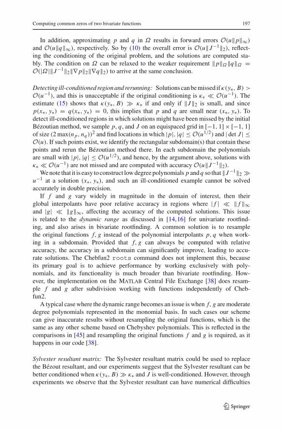
Computing common zeros of two bivariate functions 197
In addition, approximating p and q in Ω results in forward errors O(u‖p‖∞)
and O(u‖q‖∞), respectively. So by (10) the overall error is O(u‖J−1‖2), reflect-ing the conditioning of the original problem, and the solutions are computed sta-bly. The condition on Ω can be relaxed to the weaker requirement ‖p‖Ω‖q‖Ω =O(|Ω|‖J−1‖2‖∇ p‖2‖∇q‖2) to arrive at the same conclusion.
Detecting ill-conditioned region and rerunning: Solutions can be missed ifκ(y∗, B) >
O(u−1), and this is unacceptable if the original conditioning is κ∗ � O(u−1). Theestimate (15) shows that κ(y∗, B) κ∗ if and only if ‖J‖2 is small, and sincep(x∗, y∗) = q(x∗, y∗) = 0, this implies that p and q are small near (x∗, y∗). Todetect ill-conditioned regions in which solutions might have been missed by the initialBézoutian method, we sample p, q, and J on an equispaced grid in [−1, 1] × [−1, 1]of size (2 max(n p, nq))2 and find locations in which |p|, |q| ≤ O(u1/2) and | det J | ≤O(u). If such points exist, we identify the rectangular subdomain(s) that contain thesepoints and rerun the Bézoutian method there. In each subdomain the polynomialsare small with |p|, |q| ≤ O(u1/2), and hence, by the argument above, solutions withκ∗ � O(u−1) are not missed and are computed with accuracy O(u‖J−1‖2).
We note that it is easy to construct low degree polynomials p and q so that‖J−1‖2 u−1 at a solution (x∗, y∗), and such an ill-conditioned example cannot be solvedaccurately in double precision.
If f and g vary widely in magnitude in the domain of interest, then theirglobal interpolants have poor relative accuracy in regions where | f | � ‖ f ‖∞and |g| � ‖g‖∞, affecting the accuracy of the computed solutions. This issueis related to the dynamic range as discussed in [14,16] for univariate rootfind-ing, and also arises in bivariate rootfinding. A common solution is to resamplethe original functions f, g instead of the polynomial interpolants p, q when work-ing in a subdomain. Provided that f, g can always be computed with relativeaccuracy, the accuracy in a subdomain can significantly improve, leading to accu-rate solutions. The Chebfun2 roots command does not implement this, becauseits primary goal is to achieve performance by working exclusively with poly-nomials, and its functionality is much broader than bivariate rootfinding. How-ever, the implementation on the Matlab Central File Exchange [38] does resam-ple f and g after subdivision working with functions independently of Cheb-fun2.
A typical case where the dynamic range becomes an issue is when f, g are moderatedegree polynomials represented in the monomial basis. In such cases our schemecan give inaccurate results without resampling the original functions, which is thesame as any other scheme based on Chebyshev polynomials. This is reflected in thecomparisons in [45] and resampling the original functions f and g is required, as ithappens in our code [38].
Sylvester resultant matrix: The Sylvester resultant matrix could be used to replacethe Bézout resultant, and our experiments suggest that the Sylvester resultant can bebetter conditioned when κ(y∗, B) κ∗ and J is well-conditioned. However, throughexperiments we observe that the Sylvester resultant can have numerical difficulties
123
198 Y. Nakatsukasa et al.
when many solutions align along one coordinate direction, whereas the Bézout resul-tant does not. Since the Sylvester matrix polynomial is not symmetric the form of itsleft eigenvectors are nontrivial and so its conditioning is more difficult to analyze.
We also note that once subdivision is employed to yield systems of low-degreepolynomials, we can employ other methods to compute their common zeros, includ-ing those discussed in Sect. 2. We have chosen the Bézout resultant because it is theonly method whose conditioning is fully understood. The conditioning of other resul-tants have been analyzed, but less deterministically: for example, Jónsson and Vavasisanalyze the conditioning of the Macaulay resultant using probabilistic arguments [28].A detailed comparison with other approaches is beyond the scope of this paper.
6 Bézoutian regularization
The resultant, det(B(y)), is zero in exact arithmetic at precisely the y-values of thecommon zeros of p and q.
However, problematically, B(y) can be numerically singular, i.e., ‖B(y)‖2‖B(y)−1
‖2 ≥ 1015, for many values of y. A backward stable eigensolver, such as the QZalgorithm applied to a linearization of B(y), can give spurious eigenvalues of B(y)
anywhere in C [4, Sec 8.7.4], and they can cause catastrophic ill-conditioning of theother eigenvalues [40, Ch. 13].
Consequently the computed solutions can be inaccurate or spurious, and as a remedywe apply a regularization step to B(y).
6.1 Numerical singularity of Bézout matrices
The functions f and g are assumed to be smooth, and therefore, their polynomialinterpolants p and q, typically, have tensor Chebyshev expansions as in (2) withcoefficient matrices P and Q with rapidly decaying entries. Hence, the polynomi-als py(x) and qy(x) have rapidly decaying Chebyshev coefficients, and the Bézoutmatrix B(y0), for any y0 ∈ [−1, 1], inherits a similar decay as P and Q throughits definition (6). In this Sect. B(y) always denotes the matrix polynomial, whereasB(y0) is its evaluation (a symmetric matrix) at y0, which is any fixed value in[−1, 1].
The decaying entries of B(y0) mean its entries in the last column are O(u)
or smaller in magnitude. Hence eN = [0, . . . , 0, 1]T is numerically an eigen-vector with zero eigenvalue. Similar reasoning indicates that all the canonicalvectors eN , eN−1, . . . , eN−k+1 for some 1 ≤ k < N are also numericallynearly an eigenvector with zero eigenvalue. Hence, an approximate null spaceof B(y) is approximately S, where S = [
eN−k+1|eN−k+2| . . . |eN], 1 ≤ k <
N . This argument makes no reference to y0, and so we have ‖B(y0)S‖2 �‖B(y0)‖2 for any y0 ∈ [−1, 1]. Thus the matrix polynomial B(y) is closeto singular. Note that such approximate eigenpairs of B(y0) are an artifact offinite precision arithmetic, and have nothing to do with the true eigenpairs ofthe matrix polynomial B(y). By contrast, at the eigenvalues y∗ ∈ [−1, 1] ofB(y), B(y∗) has a nontrivial null space with a null vector in Vandermonde form
123
Computing common zeros of two bivariate functions 199
[T0(x∗), . . . , TN−1(x∗)
]T , which coincides with the eigenvector of the matrix poly-nomial B(y) at the eigenvalue y∗. Consequently, B(y∗) has a null vector far fromspan(S), which the numerical null space of B(y0) does not contain for other values ofy0.
6.2 Regularization details
First we partition B(y) into four parts,
B(y) =[
B1(y) E(y)T
E(y) B0(y)
], (19)
where B0(y) and E(y) are k× k and k× (N − k), respectively. We choose k to be thelargest integer so that the matrix polynomial B1(y) is numerically nonsingular for atleast one y0 ∈ [−1, 1]:
‖B0(y0)‖2 = O(u), ‖E(y0)‖2 = O(u1/2).
Note that although the bottom-right part of B(y) is of norm O(u), E(y) is typicallynot of that size; but we can still justify working with B1(y) by showing the eigenvaluesof B1(y) in y ∈ [−1, 1] are close to the eigenvalues of B(y). For our analysis thesymmetry of B(y) is crucial, and this is another reason we use Bézoutians instead ofthe Sylvester matrix.
Recall that the eigenvalues of a regular matrix polynomial B(y) are the values y∗for which the matrix B(y∗) is singular. We show that for any eigenvalue y∗ ∈ [−1, 1]of B(y), the matrix B1(y∗) with k chosen as above is nearly singular, that is, B1(y∗)has an eigenvalue of size O(u). Numerically, this means that y∗ can be computedstably via the regularized polynomial eigenvalue problem B1(y).
First, we argue that for any given y0 ∈ [−1, 1], the matrix B(y0) has at least keigenvalues of size O(u). One way to see this is to introduce
B(y) =[
B1(y) ET (y)
E(y) 0
], (20)
and note that by Weyl’s theorem, the matrix B(y0) has eigenvalues within ‖B0(y0)‖2 =O(u) of those of B(y0). Moreover, by [32, Thm. 3.1], B(y) has at least k eigenvaluesthat match those of −E(y0)
T B1(y0)−1 E(y0) up to O(‖E(y0)‖42) = O(u2). Hence, it
suffices to show that ‖E(y0)T B1(y0)
−1 E(y0)‖2 = O(u).To see why we might expect ‖E(y0)
T B1(y0)−1 E(y0)‖2 = O(u), consider the
L DLT factorization B1(y0) = L DLT , where L is unit lower triangular. For notationalsimplicity, we write L and D instead of L(y0) and D(y0). We expect that the L factorhas decaying off-diagonal elements, and D has decaying diagonals.4 To see why,
4 Strictly speaking, D needs to be allowed to have 2 × 2 blocks, since an L DLT factorization with Ddiagonal may not exist, as the example
[ 0 11 0
]illustrates. It is possible to extend the argument to such cases,
123
200 Y. Nakatsukasa et al.
consider the first step in the L DLT factorization. The first column of L is parallelto that of B1(y0), which has decaying coefficients. The Schur complement is the(n − 1)× (n − 1) matrix B1,1(y0)− d1
T , where B1,1(y0) is the lower-right part ofB1(y0), and ∈ R
n−1 is the bottom part of L’s first column. Now since has decayingcoefficients, so does the matrix d1
T , and hence the decay property is inherited byB1,1(y0) − d1
T . The rest of the L DLT factorization performs the same operationon B1,1(y0)− d1
T , so the claim follows by repeating the argument, observing thatthe diagonals of D become smaller as the factorization proceeds.
We have B−11 = L−T D−1L−1 so ET B−1
1 E = ET L−T D−1L−1 E , and since theelements of E decay towards the bottom-right corner, so do those of L−1 E . Meanwhile,the diagonals of D−1 grow towards the bottom-right, and the large elements of D−1
are multiplied by the small elements of E , so that ‖ET B−11 E‖2 � ‖E‖2‖B−1
1 ‖2.Indeed, in practice, we generally observe that ‖ET B−1
1 E‖2 = O(‖E‖22) = O(u).The remaining task is to show that B1(y∗) has an eigenvalue of size O(u) if the
numerical null space of B(y∗) has dimension k + 1.To show that B1(y∗) has an eigenvalue of size O(u), we invoke the Cauchy inter-
lacing theorem [40, Ch. 10]: arranging the eigenvalues of B1(y0) and B(y0) in non-decreasing order,
λi (B1(y0)) ≥ λi (B(y0)).
Hence λi (B(y0)) is at least as small as λi (B1(y0)). An analogous identity also holdsfor the largest eigenvalues: the i th largest eigenvalue of B(y0) is at least as large asthat of B1(y0). Consequently, an eigenvalue λi of B1(y0) with |λi | > ‖B0(y0)‖2 canonly increase in absolute value since E can be seen as a perturbation in B(y0) in (20).Since ‖B0(y0)‖2 = O(u), this means that if B(y∗) has an additional null space relativeto B(y0) at other values of y0 ∈ [−1, 1], then B1(y∗) must have an eigenvalue of sizeO(u). This shows that the y-values for which B(y) has an extra null space can bereliably detected via solving the smaller problem B1(y).
The argument above holds when the coefficients of B(y) decay, a property inheritedfrom p and q. Otherwise, ‖B0(y)‖2 and ‖E(y)‖2 are not negilible and we solve thepolynomial eigenvalue problem for B(y) without regularization. Typically, in thisscenario B(y) is not numerically singular.
Note that our regularization is not equivalent to cutting off the high-degree terms inp(x, y) and q(x, y); instead, it cuts off high-degree terms in the Bézoutian (6). We alsonote that although the initial motivation for regularizing B(y) was for stability, it alsoresults in improved efficiency because the polynomial eigenvalue problem becomessmaller in size and lower in degree.
Footnote 4 continuedbut most symmetric matrices do permit D to be diagonal, and our purpose is to explain the behavior observedin practice.
123
Computing common zeros of two bivariate functions 201
7 Further implementation details
Some further details remain and we discuss them in this section.
7.1 Construction of Bézout matrices
Our construction of (Chebyshev) Bézout matrices is based on the Matlab code givenin [39], which exploits a connection between Bézout matrices and the block symmetriclinearization of scalar and matrix polynomials. We have improved the efficiency of thatcode by restricting it to only construct Chebyshev Bézout matrices. More specifically,in [39] it was shown that if u(x) is of degree d and v(x) is of degree at most d−1, thenin the family of linearizations introduced in [33] there is a d × d symmetric pencil ofthe form λX + Y such that X is the Bézout matrix of u and v. Therefore, the Bézoutmatrix B(y0) can be obtained from py0(x) and qy0(x) in (5), providing the ability tocompute B(y0) for any y0 ∈ [−1, 1].
Let m ps and mqs be the degrees of p and q in y in the subdivided domain. Then, the
coefficient matrices Ai in B(y) = ∑m ps+mqsi=0 Ai Ti (y) can be obtained by sampling
B(y) at m ps +mqs + 1 Chebyshev points in the subdivided y-interval and convertingthem to Chebyshev coefficients using the fast Fourier transform.
7.2 Finding the eigenvalues of B(y) via linearization
Once the Chebyshev coefficients are obtained, we solve the polynomial eigenvalueproblem via the standard approach of linearization. As in Chebfun, we use the col-league matrix pencil [50, Ch. 18] for matrix polynomials, the standard companion-likelinearization for the Chebyshev basis.
After forming the coefficient matrices of B(y), we remove the leading coefficientswith Frobenius norms smaller than u maxi ‖Ai‖F , where Ai are as in (7). An analogoustechnique is used in the 1D Chebfun, and since this can be regarded as a small normwiseperturbation, it can be done without causing instability issues. The size of the pencil is(dimension of B1(y))·(degree of B1(y)) as summarized in Table 1, but regularizationand truncation can reduce the size.
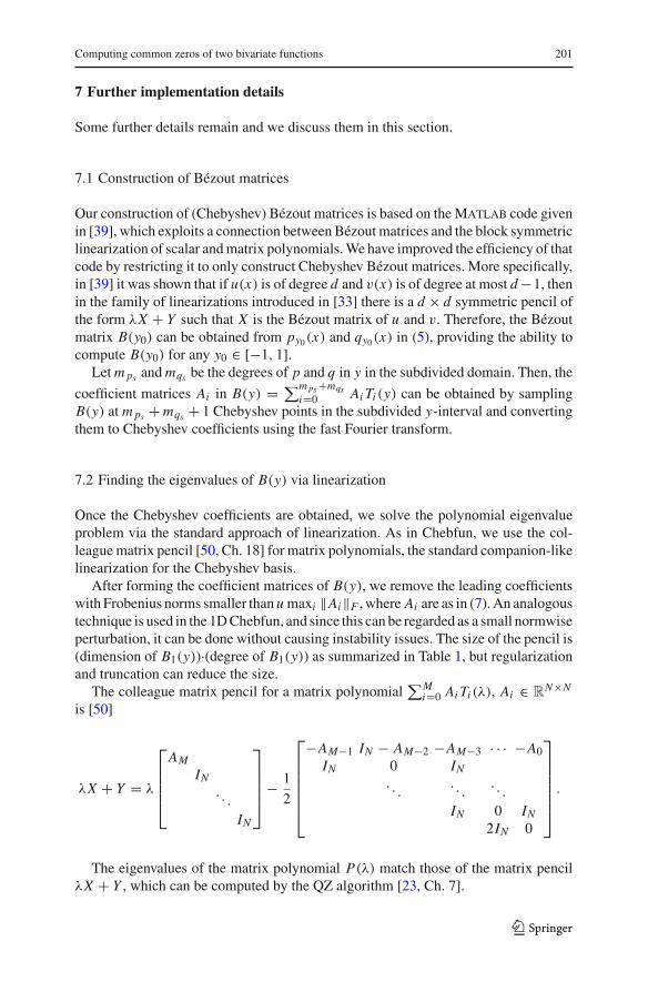
The colleague matrix pencil for a matrix polynomial∑M
i=0 Ai Ti (λ), Ai ∈ RN×N
is [50]
λX + Y = λ
⎡⎢⎢⎢⎣
AM
IN. . .
IN
⎤⎥⎥⎥⎦−
1
2
⎡⎢⎢⎢⎢⎢⎣
−AM−1 IN − AM−2 −AM−3 · · · −A0IN 0 IN
. . .. . .
. . .
IN 0 IN
2IN 0
⎤⎥⎥⎥⎥⎥⎦
.
The eigenvalues of the matrix polynomial P(λ) match those of the matrix pencilλX + Y , which can be computed by the QZ algorithm [23, Ch. 7].
123
202 Y. Nakatsukasa et al.
7.3 Univariate rootfinding
Once we have found the y-values of the solutions, then we find the x-values by aunivariate rootfinding algorithm based on computing the eigenvalues of the colleaguematrix [50], and using the eig command in Matlab. Due to subdivision, the poly-nomials are of degree≤ 16 on each subregion, and computing their roots is negligiblein cost.
We compute the roots of both p(x, y∗) and q(x, y∗) on the subdivided x-intervalseparately and numerically verify that the absolute values of p and q are less than acertain tolerance at these solutions, discarding those that are not. The exact tolerancewe take depends on whether we are seeking an initial estimate or performing a localrefinement (see Subsect. 7.4). Afterwards, we merge any x-values that are closer thana distance of O(u) apart by averaging to prevent double-counting a solution due torounding errors.
7.4 Local Bézoutian refinement
This component is crucial to the success of the algorithm. After computing the approxi-mate solutions via the initial Bézoutians we further employ highly localized Bézoutiansnear the solutions for improved stability and accuracy. Specifically, we do the follow-ing:
1. Group the computed zeros into clusters, each of whose members are withinO(u1/4)
in Hausdorff distance; and2. For each cluster, execute another Bézout-based rootfinder in a small domain of
width O(u1/4) that contains the cluster.
The distance u1/4 was chosen so as to be small enough not to contain too many solu-tions, and large enough to accommodate the errors in the initially computed solutions.The local Bézoutian refinement is beneficial to prevent the conditioning worsening(see Sect. 5), spurious, multiply-counted, and inaccurate solutions. The task of theinitial global Bézoutian is to obtain an estimate of the solutions that are allowed tohave error larger than O(u), but must not be missed. Hence, at first we accept x-valueswith | f (x∗, y∗)|, |g(x∗, y∗)| ≤ O(u1/2), which does not remove those correspondingto near-multiple or ill-conditioned solutions, and then during the local refinement wedo a more stringent test requiring | f | and |g| to be O(u).
Since at the local level the domain is much smaller than the original, the polynomialinterpolants of f and g are of very low degree, and hence the overhead in cost ismarginal.
Sometimes the local domain is so small that one of the polynomials, say p, isnumerically constant in one (or both) variable, say x . In such cases we trivially findthe roots y∗ of p(y) and compute the roots of q(x, y∗) on the local interval.
Local refinement usually results in a significant improvement in accuracy as dis-cussed in Sect. 5. Moreover, the low-degree polynomials result in a Bézout matrixpolynomial B(y) that is far from singular, and so its numerical solution can be carriedout stably.
123
Computing common zeros of two bivariate functions 203
The refinement is vital when many solutions exist with nearly the same value in thefirst coordinate y. For example, suppose that (xi , y0 + δi ) for i = 1, . . . , k are simplezeros of f and g, where |δi | are small. Then the computed eigenvalues of the Bézoutmatrix polynomial take many (at least k) values close to y0. The algorithm then findsthe corresponding x-values via a univariate rootfinder, but this process faces difficulty,as for each computed y0 + δi , the two functions f (x, y0 + δi ) and g(x, y0 + δi ) havek nearly multiple zeros, and this can result in counting the same zero multiple times.The local Bézout refinement resolves this by regarding such multiply counted zerosas a cluster and working in a subdomain that contains very few common zeros.
7.5 Solutions off the domain, but numerically close
Some care is required to avoid missing solutions that lie on or near the boundary of thedomain [−1, 1] × [−1, 1], as a small backward perturbation can move them outside.This is the same reason we do not exactly bisect in the subdivision (see Sect. 4).We must also be careful not to miss real solutions that are numerically perturbed tocomplex ones with negligible imaginary parts.
To ensure that we do not miss the solutions near the boundary, we initially lookfor solutions in the slightly enlarged domain [−1 − δ, 1 + δ] × [−1 − δ, 1 + δ],where δ = 10−10. Then we disregard solutions outside [−1, 1] × [−1, 1]. Solutionsoff the domain within a distance of 10−15 are regarded as solutions on the boundaryby perturbing them.
To capture solutions that have been numerically perturbed to have negligible imag-inary parts we check for the eigenvalues of B(y) with real parts in [−1, 1] × [−1, 1]and the imaginary parts of size O(u1/2), or smaller. The tolerance of size O(u1/2)
is reasonable since two numerically close common zeros can be perturbed into thecomplex plane by this amount.
7.6 Spurious zeros and their removal
One difficulty with resultant-based bivariate rootfinders is spurious zeros, which arey-values for which the resultant is numerically singular, but p and q do not have acommon zero in the domain of interest.
There are several ways spurious zeros can arise: (i) A shared zero at infinity, forexample, if deg p > deg q in x then there is a spurious zero at values of y for whichthe leading coefficient of p is zero; (ii) An exact nonreal common zero or an exact realcommon zero lying outside the domain; and (iii) Numerical artifacts that arise due tothe ill-conditioning of B(y).
Fortunately, a computed spurious zero arising before local refinement will revealitself when we refine. There are two reasons why refinement removes spurious zeros.First, refinement reduces the degree of the polynomial approximants, meaning it isless likely to encounter shared zeros at infinity. Second, the matrix polynomial B(y)
is smaller in both size and degree and typically has a greatly improved conditionnumber. In the unlikely event that a spurious zero is present in the final stage, univariate
123
204 Y. Nakatsukasa et al.
rootfinding performs an additional control to check that we have the common zerosof the original bivariate functions.
The above qualitative arguments suggest, and experiments corroborate, that localrefinement is an effective approach for the removal of spurious zeros, a well-knownchallenge for resultant-based methods. Although in theory spurious zeros can stillarise, we are not aware of an example where local refinement fails to remove them.
8 Numerical examples
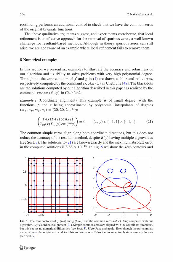
In this section we present six examples to illustrate the accuracy and robustness ofour algorithm and its ability to solve problems with very high polynomial degree.Throughout, the zero contours of f and g in (1) are drawn as blue and red curves,respectively, computed by the command roots(f) in Chebfun2 [48]. The black dotsare the solutions computed by our algorithm described in this paper as realized by thecommand roots(f,g) in Chebfun2.
Example 1 (Coordinate alignment) This example is of small degree, with thefunctions f and g being approximated by polynomial interpolants of degrees(m p, n p, mq , nq) = (20, 20, 24, 30):
(T7(x)T7(y) cos(xy)
T10(x)T10(y) cos(x2 y)
)= 0, (x, y) ∈ [−1, 1] × [−1, 1]. (21)
The common simple zeros align along both coordinate directions, but this does notreduce the accuracy of the resultant method, despite B(y) having multiple eigenvalues(see Sect. 3). The solutions to (21) are known exactly and the maximum absolute errorin the computed solutions is 8.88 × 10⁻¹⁶. In Fig. 5 we show the zero contours and
−1 −0.5 0 0.5 1−1
−0.5
0
0.5
1
−2 −1 0 1 2
−1
0
1
2
3
4
Fig. 5 The zero contours of f (red) and g (blue), and the common zeros (black dots) computed with ouralgorithm. Left Coordinate alignment (21). Simple common zeros are aligned with the coordinate directions,but this causes no numerical difficulties (see Sect. 3). Right Face and apple. Even though the polynomialsare small near the origin we can detect this and use a local Bézout refinement to obtain accurate solutions(see Sect. 7)
123
Computing common zeros of two bivariate functions 205
common zeros for (21). The zero contour lines quadratically cluster near the edge ofthe domain following the distribution of the roots of Chebyshev polynomials.
Example 2 (Face and apple) Here, we select functions f and g that are exactly poly-nomials, i.e., f = p and g = q, with zero contours suggesting a face and an apple,respectively. These bivariate polynomials were taken from [42], and the degrees are(m p, n p, mq , nq) = (10, 18, 8, 8). Note that in this example we have taken the domain[−2, 2] × [−1.5, 4].
This example is of mathematical interest because both polynomials are relativelysmall ≤ 10−5 near the origin where the Bézout resultant can severely worsen thecondition number of the solutions. Such solutions can be initially missed, and torecover them the code detects ill-conditioned subdomains and reruns the Bézoutianthere (see Sect. 5.1).
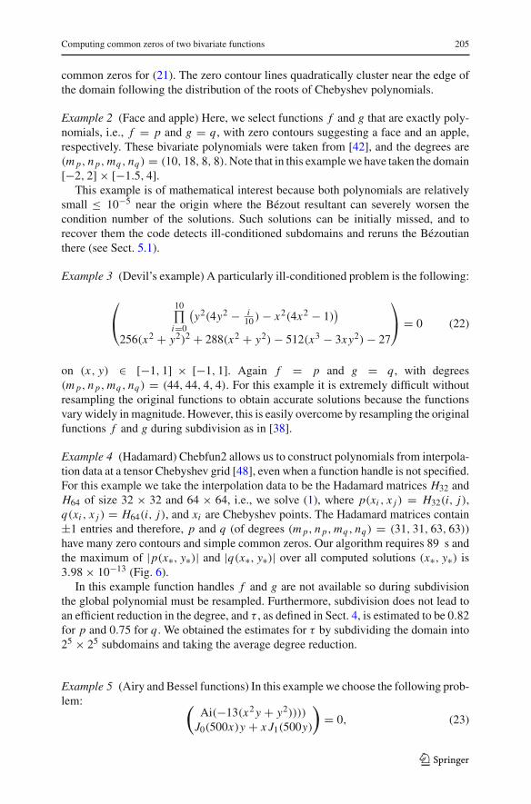
Example 3 (Devil’s example) A particularly ill-conditioned problem is the following:
⎛⎝
10∏i=0
(y2(4y2 − i
10 )− x2(4x2 − 1))
256(x2 + y2)2 + 288(x2 + y2)− 512(x3 − 3xy2)− 27
⎞⎠ = 0 (22)
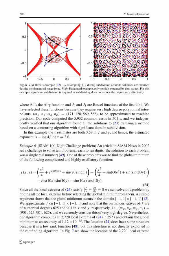
on (x, y) ∈ [−1, 1] × [−1, 1]. Again f = p and g = q, with degrees(m p, n p, mq , nq) = (44, 44, 4, 4). For this example it is extremely difficult withoutresampling the original functions to obtain accurate solutions because the functionsvary widely in magnitude. However, this is easily overcome by resampling the originalfunctions f and g during subdivision as in [38].
Example 4 (Hadamard) Chebfun2 allows us to construct polynomials from interpola-tion data at a tensor Chebyshev grid [48], even when a function handle is not specified.For this example we take the interpolation data to be the Hadamard matrices H32 andH64 of size 32 × 32 and 64 × 64, i.e., we solve (1), where p(xi , x j ) = H32(i, j),q(xi , x j ) = H64(i, j), and xi are Chebyshev points. The Hadamard matrices contain±1 entries and therefore, p and q (of degrees (m p, n p, mq , nq) = (31, 31, 63, 63))have many zero contours and simple common zeros. Our algorithm requires 89 s andthe maximum of |p(x∗, y∗)| and |q(x∗, y∗)| over all computed solutions (x∗, y∗) is3.98× 10−13 (Fig. 6).
In this example function handles f and g are not available so during subdivisionthe global polynomial must be resampled. Furthermore, subdivision does not lead toan efficient reduction in the degree, and τ , as defined in Sect. 4, is estimated to be 0.82for p and 0.75 for q. We obtained the estimates for τ by subdividing the domain into25 × 25 subdomains and taking the average degree reduction.
Example 5 (Airy and Bessel functions) In this example we choose the following prob-lem: (
Ai(−13(x2 y + y2))))
J0(500x)y + x J1(500y)
)= 0, (23)
123
206 Y. Nakatsukasa et al.
−1 −0.5 0 0.5 1−1
−0.5
0
0.5
1
−1 −0.5 0 0.5 1−1
−0.5
0
0.5
1
Fig. 6 Left Devil’s example (22). By resampling f, g during subdivision accurate solutions are obtaineddespite the dynamical range issue. Right Hadamard example, polynomials obtained by data values. For thisexample significant subdivision is required as subdividing does not reduce the degree very effectively
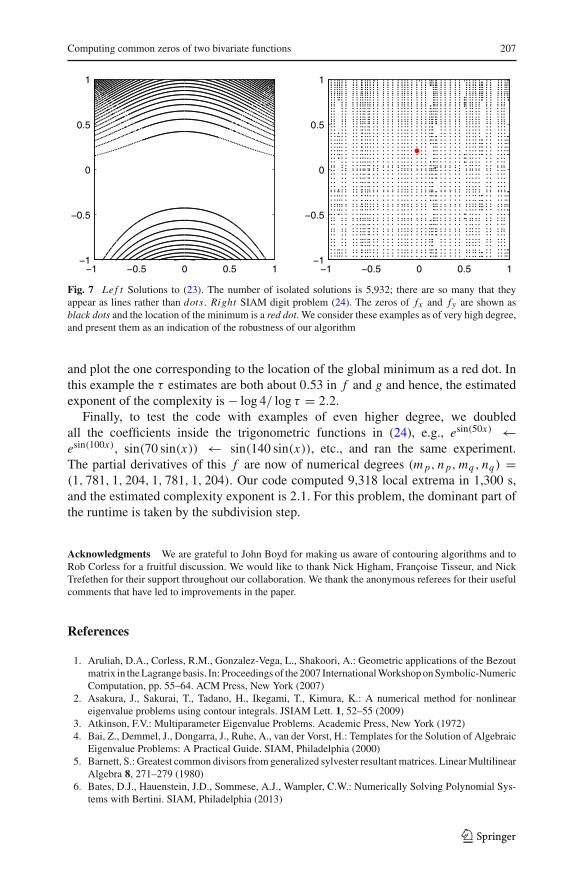
where Ai is the Airy function and J0 and J1 are Bessel functions of the first kind. Wehave selected these functions because they require very high degree polynomial inter-polants, (m p, n p, mq , nq) = (171, 120, 569, 568), to be approximated to machineprecision. Our code computed the 5,932 common zeros in 501 s, and we indepen-dently verified that our algorithm found all the solutions to (23) by using a methodbased on a contouring algorithm with significant domain subdivision.
In this example the τ estimates are both 0.59 in f and g, and hence, the estimatedexponent is − log 4/ log τ = 2.6.
Example 6 (SIAM 100-Digit Challenge problem) An article in SIAM News in 2002set a challenge to solve ten problems, each to ten digits (the solution to each problemwas a single real number) [49]. One of these problems was to find the global minimumof the following complicated and highly oscillatory function:
f (x, y) =(
x2
4+ esin(50x) + sin(70 sin(x))
)+
(y2
4+ sin(60ey)+ sin(sin(80y))
)
− cos(10x) sin(10y)− sin(10x) cos(10y).
(24)Since all the local extrema of (24) satisfy ∂ f
∂x = ∂ f∂y = 0 we can solve this problem by
finding all the local extrema before selecting the global minimum from them. A simpleargument shows that the global minimum occurs in the domain [−1, 1]×[−1, 1] [12].We approximate f on [−1, 1] × [−1, 1] and note that the partial derivatives of f areof numerical degrees 625 and 901 in x and y, respectively, i.e., (m p, n p, mq , nq) =(901, 625, 901, 625), and we currently consider this of very high degree. Nevertheless,our algorithm computes all 2,720 local extrema of (24) in 257 s and obtains the globalminimum to an accuracy of 1.12×10⁻¹⁵. The function (24) does have some structurebecause it is a low rank function [48], but this structure is not directly exploited inthe rootfinding algorithm. In Fig. 7 we show the location of the 2,720 local extrema
123
Computing common zeros of two bivariate functions 207
−1 −0.5 0 0.5 1−1
−0.5
0
0.5
1
−1 −0.5 0 0.5 1−1
−0.5
0
0.5
1
Fig. 7 Le f t Solutions to (23). The number of isolated solutions is 5,932; there are so many that theyappear as lines rather than dots. Right SIAM digit problem (24). The zeros of fx and fy are shown asblack dots and the location of the minimum is a red dot. We consider these examples as of very high degree,and present them as an indication of the robustness of our algorithm
and plot the one corresponding to the location of the global minimum as a red dot. Inthis example the τ estimates are both about 0.53 in f and g and hence, the estimatedexponent of the complexity is − log 4/ log τ = 2.2.
Finally, to test the code with examples of even higher degree, we doubledall the coefficients inside the trigonometric functions in (24), e.g., esin(50x) ←esin(100x), sin(70 sin(x)) ← sin(140 sin(x)), etc., and ran the same experiment.The partial derivatives of this f are now of numerical degrees (m p, n p, mq , nq) =(1, 781, 1, 204, 1, 781, 1, 204). Our code computed 9,318 local extrema in 1,300 s,and the estimated complexity exponent is 2.1. For this problem, the dominant part ofthe runtime is taken by the subdivision step.
Acknowledgments We are grateful to John Boyd for making us aware of contouring algorithms and toRob Corless for a fruitful discussion. We would like to thank Nick Higham, Françoise Tisseur, and NickTrefethen for their support throughout our collaboration. We thank the anonymous referees for their usefulcomments that have led to improvements in the paper.
References
1. Aruliah, D.A., Corless, R.M., Gonzalez-Vega, L., Shakoori, A.: Geometric applications of the Bezoutmatrix in the Lagrange basis. In: Proceedings of the 2007 International Workshop on Symbolic-NumericComputation, pp. 55–64. ACM Press, New York (2007)
2. Asakura, J., Sakurai, T., Tadano, H., Ikegami, T., Kimura, K.: A numerical method for nonlineareigenvalue problems using contour integrals. JSIAM Lett. 1, 52–55 (2009)
3. Atkinson, F.V.: Multiparameter Eigenvalue Problems. Academic Press, New York (1972)4. Bai, Z., Demmel, J., Dongarra, J., Ruhe, A., van der Vorst, H.: Templates for the Solution of Algebraic
Eigenvalue Problems: A Practical Guide. SIAM, Philadelphia (2000)5. Barnett, S.: Greatest common divisors from generalized sylvester resultant matrices. Linear Multilinear
Algebra 8, 271–279 (1980)6. Bates, D.J., Hauenstein, J.D., Sommese, A.J., Wampler, C.W.: Numerically Solving Polynomial Sys-
tems with Bertini. SIAM, Philadelphia (2013)
123
208 Y. Nakatsukasa et al.
7. Beyn, W.-J.: An integral method for solving nonlinear eigenvalue problems. Linear Algebra Appl.436(10), 3839–3863 (2012)
8. Bézout, É.: Théorie Générale des Équations Algébriques. PhD thesis, Pierres, Paris (1779)9. Bini, D.A., Gemignani, L.: Bernstein-bezoutian matrices. Theor. Comput. Sci. 315(2), 319–333 (2004)
10. Bini, D.A., Marco, A.: Computing curve intersection by means of simultaneous iterations. Numer.Algorithms 43, 151–175 (2006)
11. Bini, D.A., Noferini, V.: Solving polynomial eigenvalue problems by means of the Ehrlich–Aberthmethod. Linear Algebra Appl. 439, 1130–1149 (2013)
12. Bornemann, F., Laurie, D., Wagon, S., Waldvogel, H.: The SIAM 100-Digit Challenge: A Study inHigh-Accuracy Numerical Computing. SIAM, Philadelphia (2004)
13. Boyd, J.P.: Computing zeros on a real interval through chebyshev expansion and polynomial rootfind-ing. SIAM J. Numer. Anal. 40, 1666–1682 (2002)
14. Boyd, J.P.: Computing real roots of a polynomial in chebyshev series form through subdivision. Appl.Numer. Math. 56, 1077–1091 (2006)
15. Boyd, J.P.: Computing real roots of a polynomial in chebyshev series form through subdivision withlinear testing and cubic solves. Appl. Math. Comput. 174, 1642–1658 (2006)
16. Boyd, J.P., Gally, D.H.: Numerical experiments on the accuracy of the chebyshev-frobenius companionmatrix method for finding the zeros of a truncated series of chebyshev polynomials. J. Comput. Appl.Math. 205(1), 281–295 (2007)
17. Buchberger, B.: Introduction to Gröbner bases. In: Gröbner Basis and Applications, vol. 251, pp. 3–31.Cambridge University Press, Cambridge (1998)
18. Cox, D.A., Little, J.B., O’Shea, D.: Ideals, Varieties, and Algorithms: Introduction to ComputationalAlgebraic Geometry and Commutative Algebra, 3rd edn. Springer, Berlin (2007)
19. Diaz-Toca, G.M., Fioravanti, M., Gonzalez-Vega, L., Shakoori, A.: Using implicit equations of para-metric curves and surfaces without computing them: polynomial algebra by values. Comput. AidedGeom. D. 30, 116–139 (2013)
20. Dreesen, P., Batselier, K., De Moor, B.: Back to the roots: Polynomial system solving, linear algebra,systems theory. In: Proceedings of 16th IFAC Symposium on System Identification, pp. 1203–1208(2012)
21. Emiris, I.Z., Mourrai, B.: Matrices in elimination theory. J. Symb. Comput. 28, 3–44 (1999)22. Gohberg, I., Lancaster, P., Rodman, L.: Matrix Polynomials. SIAM, Philadelphia (unabridged repub-
lication of book first published by academic press in 1982) edition (2009)23. Golub, G.H., Van Loan, C.F.: Matrix Computations. The Johns Hopkins University Press, Baltimore
(1996)24. Harnack, C.G.A.: Über vieltheiligkeit der ebenen algebraischen curven. Math. Ann. 10, 189–199 (1876)25. Higham, N.J.: Accuracy and Stability of Numerical Algorithms, 2nd edn. SIAM, Philadelphia (2002)26. Hilton, A., Stoddart, A.J., Illingwort, J., Windeatt, T.: Marching triangles: range image fusion for
complex object modelling. In: International Conference on Image Processing, vol. 1 (1996)27. Hochstenbach, M.E., Košir, T., Plestenjak, B.: A jacobi-davidson type method for the two-parameter
eigenvalue problem. SIAM J. Matrix Anal. Appl. 26(2), 477–497 (2004)28. Jónsson, G., Vavasis, S.: Accurate solution of polynomial equations using macaulay resultant matrices.
Math. Comp. 74, 221–262 (2005)29. Kapur, D., Saxena, T.: Comparison of various multivariate resultant formulations. In: Levelt, A. (ed)
Proceedings of International Symposium on Symbolic and Algebraic Computation, pp. 187–194.Montreal (1995)
30. Kirwan, F.C.: Complex Algebraic Curves. Cambridge University Press, Cambridge (1992)31. Kravitsky, N.: On the discriminant function of two commuting nonselfadjoint operators. Integr. Equ.
Oper. Theory 3, 97–125 (1980)32. Li, R.-C., Nakatsukasa, Y., Truhar, N., Wang, W.: Perturbation of multiple eigenvalues of hermitian
matrices. Linear Algebra Appl. 437, 202–213 (2012)33. Mackey, D.S., Mackey, N., Mehl, C., Mehrmann, V.: Vector spaces of linearizations for matrix poly-
nomials. SIAM J. Matrix Anal. Appl. 28, 971–1004 (2006)34. Manocha, D., Demmel, J.: Algorithms for intersecting parametric and algebraic curves I: simple inter-
sections. ACM Trans. Graph. 13, 73–100 (1994)35. Marks II, R.J.: Introduction to Shannon Sampling and Interpolation Theory. Springer, New York (1991)36. Mehrmann, V., Voss, H.: Nonlinear eigenvalue problems: A challenge for modern eigenvalue methods.
Mitt. der Ges. fr Angewandte Mathematik and Mechanik 27, 121–151 (2005)
123
Computing common zeros of two bivariate functions 209
37. Muhic, A., Plestenjak, B.: On the quaratic two-parameter eigenvalue problem and its linearization.Linear Algebra Appl. 432, 2529–2542 (2010)
38. Nakatsukasa, Y., Noferini, V., Townsend, A.: Computing common zeros of two bivariate functions.MATLAB Central File Exchange (2013). http://www.mathworks.com/matlabcentral/fileexchange/44084
39. Nakatsukasa, Y., Noferini, V., Townsend, A.: Vector spaces of linearizations for matrix polynomials:a bivariate polynomial approach. Preprint (2014)
40. Parlett, B.N.: The Symmetric Eigenvalue Problem. SIAM, Philadelphia (1998)41. Plaumann, D., Sturmfels, B., Vinzant, C.: Computing linear matrix representations of Helton–Vinnikov
curves. Math. Methods Syst. Optim. Control Oper. Theory 222, 259–277 (2012)42. Sagraloff, M. et al.: Gallery of algebraic curves and their arrangements. http://exacus.mpi-inf.mpg.de/
gallery.html43. Salmon, G.: Lessons Introductory to the Modern Higher Algebra. G. E. Stechert & Co., New York
(1885)44. Sommese, A.J., Wampler, C.W.: The Numerical Solution of Systems of Polynomials. World Scientific,
Singapore (2005)45. Sorber, L., Van Barel, M., De Lathauwer, L.: Numerical solution of bivariate and polyanalytic poly-
nomial systems. Preprint (2013)46. Sun, J.-G.: On condition numbers of a nondefective multiple eigenvalue. Numer. Math. 61, 265–275
(1992)47. Tisseur, F.: Backward error and condition of polynomial eigenvalue problems. Linear Algebra Appl.
309, 339–361 (2000)48. Townsend, A., Trefethen, L.N.: An extension of chebfun to two dimensions. SIAM J. Sci. Comput.
35(6), C495–C518 (2013)49. Trefethen, L.N.: A hundred-dollar, hundred-digit challenge. SIAM News, 35 (2002)50. Trefethen, L.N.: Approximation Theory and Approximation Practice. SIAM, Philadelphia (2013)51. Trefethen, L.N. et al.: Chebfun version 4.2.2949. Software. The Chebfun Development Team (2013)52. Wilkinson, J.H.: The perfidious polynomial. In: Golub, G.H. (ed) Studies in Numerical Analysis.
Mathematical Association of America (1984)53. Xie, H., Dai, H.: On the sensitivity of multiple eigenvalues of nonsymmetric matrix pencils. Linear
Algebra Appl. 374, 143–158 (2003)
123