Computing Simulations in SAS

Jordan Elm7/26/2007

Reference:SAS for Monte Carlo Studies: A Guide for Quantitative Researchers by Xitao Fan, Akos Felsovalyi, Stephen Sivo, and Sean Keenan Copyright(c) 2002 by SAS Institute Inc., Cary, NC, USA

What is meant by “Running Simulations”

Simulating Data- Use Random Number Generator. To generate data with certain

distribution/shape. Monte Carlo Simulations- Use

Random Number Generator, Do Loops, Macros To generate data and compare

performance of different methods of analysis.

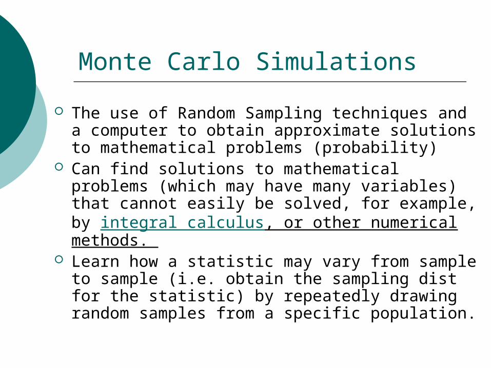
Monte Carlo Simulations

The use of Random Sampling techniques and a computer to obtain approximate solutions to mathematical problems (probability)

Can find solutions to mathematical problems (which may have many variables) that cannot easily be solved, for example, by integral calculus, or other numerical methods.

Learn how a statistic may vary from sample to sample (i.e. obtain the sampling dist for the statistic) by repeatedly drawing random samples from a specific population.

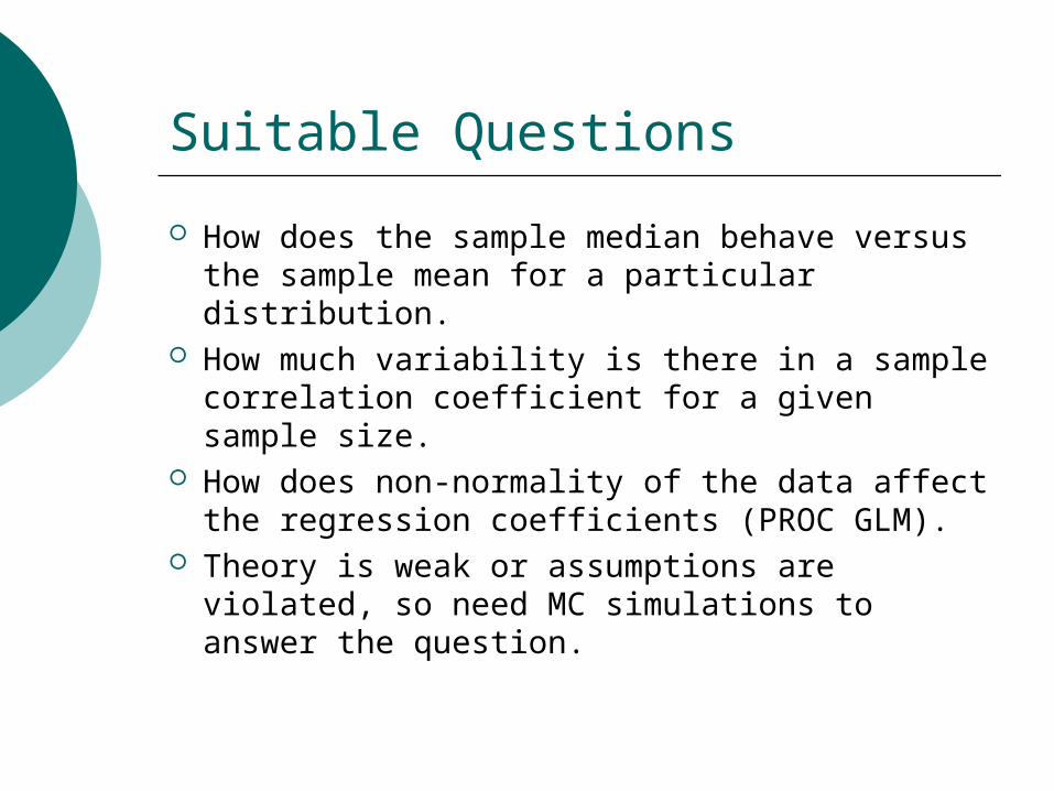
Suitable Questions

How does the sample median behave versus the sample mean for a particular distribution.

How much variability is there in a sample correlation coefficient for a given sample size.

How does non-normality of the data affect the regression coefficients (PROC GLM).

Theory is weak or assumptions are violated, so need MC simulations to answer the question.

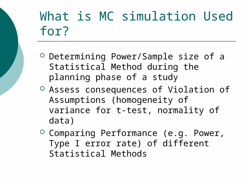
What is MC simulation Used for?

Determining Power/Sample size of a Statistical Method during the planning phase of a study

Assess consequences of Violation of Assumptions (homogeneity of variance for t-test, normality of data)

Comparing Performance (e.g. Power, Type I error rate) of different Statistical Methods

Example: Rolling the Die Twice

What are the chances of obtaining 2 as the sum of rolling a die twice?

1. Roll die twice 10,000 times by hand so can estimate the chance of obtaining 2 as the sum.

2. Apply probability theory (1/6*1/6)=0.0283. Empirical Approach –Monte Carlo Simulation

The outcomes of rolling a die are SIMULATED. Requires a computer and software (SAS, Stata R).

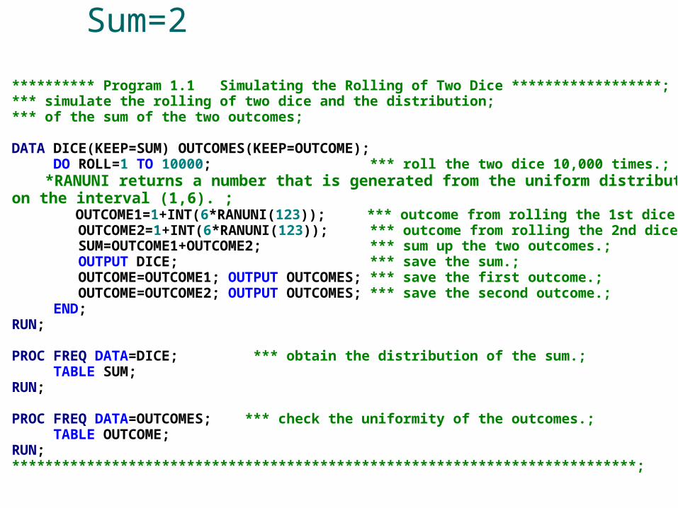
Rolling Die Twice: Prob Sum=2

********** Program 1.1 Simulating the Rolling of Two Dice ******************; *** simulate the rolling of two dice and the distribution; *** of the sum of the two outcomes; DATA DICE(KEEP=SUM) OUTCOMES(KEEP=OUTCOME); DO ROLL=1 TO 10000; *** roll the two dice 10,000 times.; *RANUNI returns a number that is generated from the uniform distribution on the interval (1,6). ; OUTCOME1=1+INT(6*RANUNI(123)); *** outcome from rolling the 1st dice; OUTCOME2=1+INT(6*RANUNI(123)); *** outcome from rolling the 2nd dice; SUM=OUTCOME1+OUTCOME2; *** sum up the two outcomes.; OUTPUT DICE; *** save the sum.; OUTCOME=OUTCOME1; OUTPUT OUTCOMES; *** save the first outcome.; OUTCOME=OUTCOME2; OUTPUT OUTCOMES; *** save the second outcome.; END; RUN; PROC FREQ DATA=DICE; *** obtain the distribution of the sum.; TABLE SUM; RUN; PROC FREQ DATA=OUTCOMES; *** check the uniformity of the outcomes.; TABLE OUTCOME; RUN; ***************************************************************************;

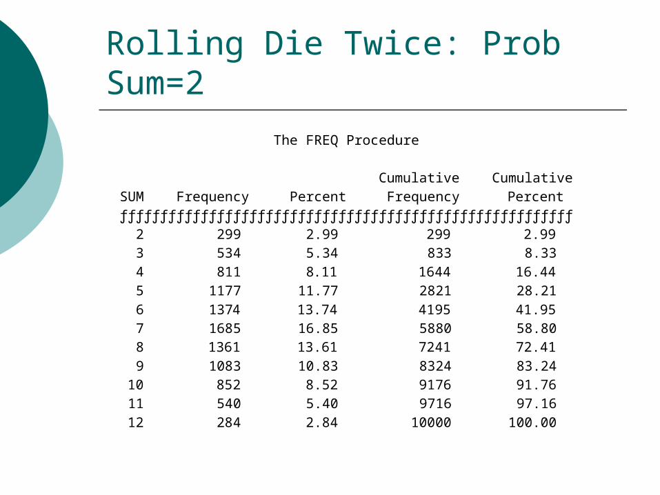
The FREQ Procedure Cumulative Cumulative SUM Frequency Percent Frequency Percent ƒƒƒƒƒƒƒƒƒƒƒƒƒƒƒƒƒƒƒƒƒƒƒƒƒƒƒƒƒƒƒƒƒƒƒƒƒƒƒƒƒƒƒƒƒƒƒƒƒƒƒƒƒƒƒƒ 2 299 2.99 299 2.99 3 534 5.34 833 8.33 4 811 8.11 1644 16.44 5 1177 11.77 2821 28.21 6 1374 13.74 4195 41.95 7 1685 16.85 5880 58.80 8 1361 13.61 7241 72.41 9 1083 10.83 8324 83.24 10 852 8.52 9176 91.76 11 540 5.40 9716 97.16 12 284 2.84 10000 100.00

Rolling Die Twice: Prob Sum=2

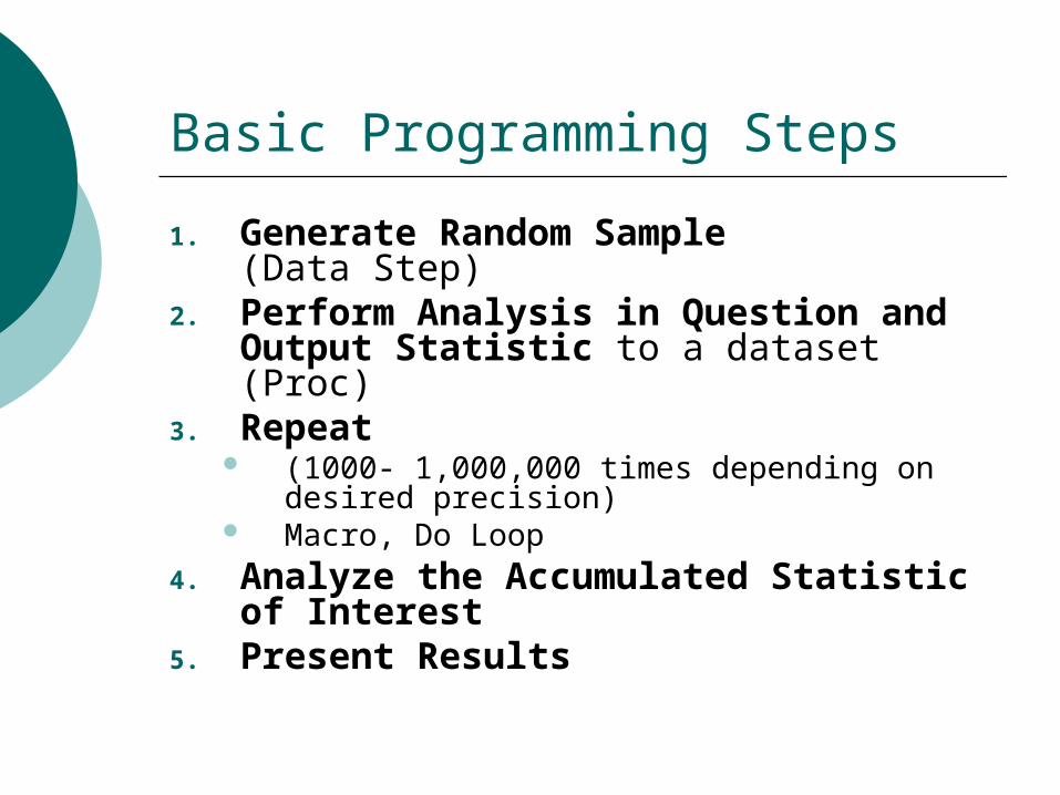
Basic Programming Steps

1. Generate Random Sample (Data Step)

2. Perform Analysis in Question and Output Statistic to a dataset (Proc)

3. Repeat (1000- 1,000,000 times depending on desired

precision) Macro, Do Loop

4. Analyze the Accumulated Statistic of Interest

5. Present Results

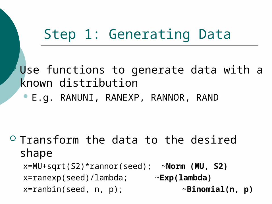
Step 1: Generating Data

Use functions to generate data with a known distribution E.g. RANUNI, RANEXP, RANNOR, RAND

Transform the data to the desired shapex=MU+sqrt(S2)*rannor(seed); ~Norm (MU, S2)x=ranexp(seed)/lambda; ~Exp(lambda)x=ranbin(seed, n, p); ~Binomial(n, p)

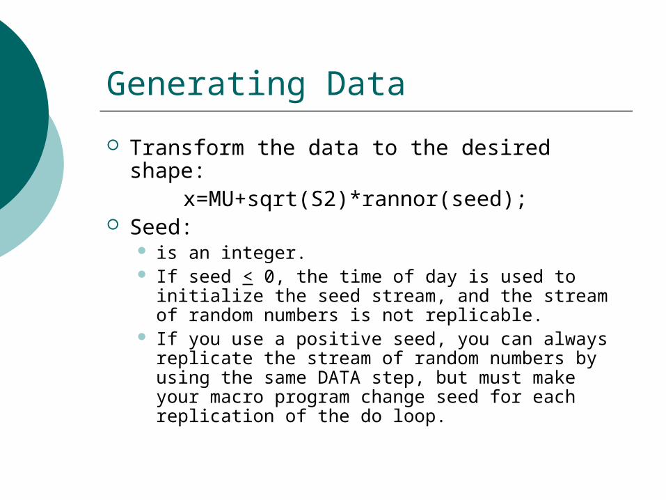
Generating Data

Transform the data to the desired shape: x=MU+sqrt(S2)*rannor(seed); Seed:

is an integer. If seed < 0, the time of day is used to initialize

the seed stream, and the stream of random numbers is not replicable.

If you use a positive seed, you can always replicate the stream of random numbers by using the same DATA step, but must make your macro program change seed for each replication of the do loop.

Generating Data

Multivariate data: %MVN macro Download fromhttp://support.sas.com/ctx/samples/index.jsp?sid=509

Tip for faster program: Generate ALL the data first, then use the BY

statement within PROC to analyze each “sample”.

E.g. If sample size is 50 and # of reps is set to 1000, then generate data with 50000 obs.

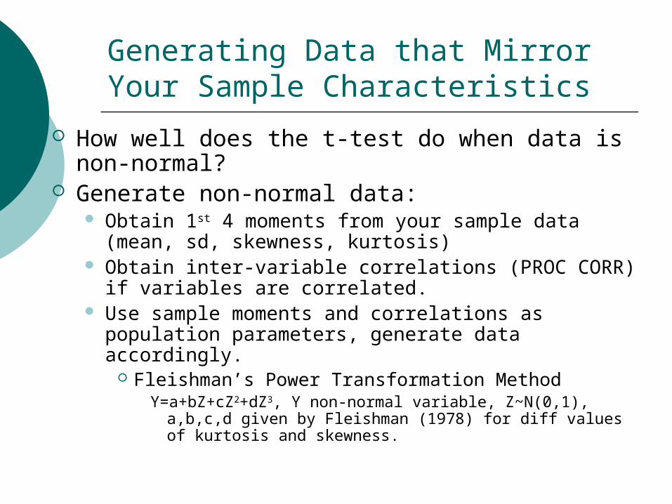
Generating Data that Mirror Your Sample Characteristics

How well does the t-test do when data is non-normal?

Generate non-normal data: Obtain 1st 4 moments from your sample data (mean,

sd, skewness, kurtosis) Obtain inter-variable correlations (PROC CORR) if

variables are correlated. Use sample moments and correlations as population

parameters, generate data accordingly. Fleishman’s Power Transformation Method

Y=a+bZ+cZ2+dZ3, Y non-normal variable, Z~N(0,1), a,b,c,d given by Fleishman (1978) for diff values of kurtosis and skewness.

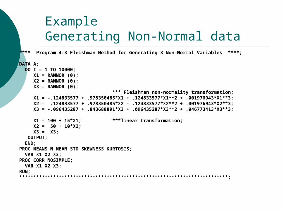
Example Generating Non-Normal data

**** Program 4.3 Fleishman Method for Generating 3 Non-Normal Variables ****;

DATA A; DO I = 1 TO 10000; X1 = RANNOR (0); X2 = RANNOR (0); X3 = RANNOR (0); *** Fleishman non-normality transformation; X1 = -.124833577 + .978350485*X1 + .124833577*X1**2 + .001976943*X1**3; X2 = .124833577 + .978350485*X2 - .124833577*X2**2 + .001976943*X2**3; X3 = -.096435287 + .843688891*X3 + .096435287*X3**2 + .046773413*X3**3;

X1 = 100 + 15*X1; ***linear transformation; X2 = 50 + 10*X2; X3 = X3; OUTPUT; END;PROC MEANS N MEAN STD SKEWNESS KURTOSIS; VAR X1 X2 X3;PROC CORR NOSIMPLE; VAR X1 X2 X3;RUN;**************************************************************************;

Example of MC study

Assessing the effect of Non-normal data on the Type I error rate of an ANOVA test

Proc IML

Matrix Language within SAS

Allows for faster programming, however, still slower than Stata, R, S-plus.

Program 6.3: Assessing the effect of Data Non-Normality on the Type I error rate in ANOVA

Bootstrapping & Jackknifing

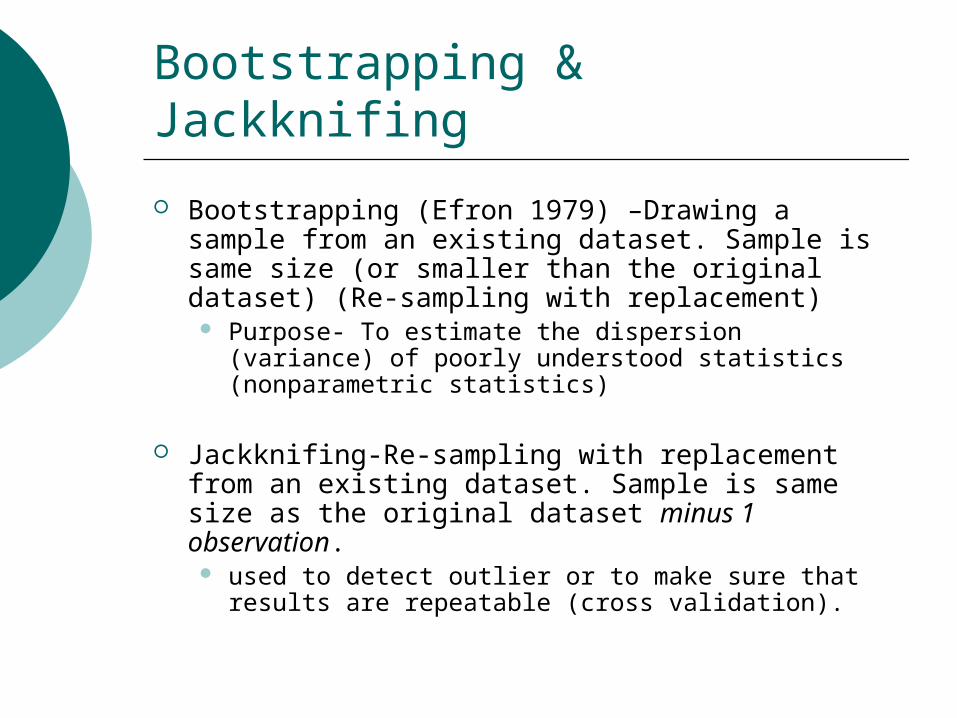
Bootstrapping (Efron 1979) –Drawing a sample from an existing dataset. Sample is same size (or smaller than the original dataset) (Re-sampling with replacement) Purpose- To estimate the dispersion (variance) of

poorly understood statistics (nonparametric statistics)

Jackknifing-Re-sampling with replacement from an existing dataset. Sample is same size as the original dataset minus 1 observation. used to detect outlier or to make sure that results

are repeatable (cross validation).

Examples of Simulation Examples of Simulation Studies in EpidemiologyStudies in Epidemiology

Simulation Study of Confounder-Selection StrategiesG Maldonado, S Greenland American Journal of Epidemiology Vol. 138, No. 11: 923-936

In the absence of prior knowledge about population relations, investigators frequently employ a strategy that uses the data to help them decide whether to adjust for a variable. The authors compared the performance of several such strategies for fitting multiplicative Poisson regression models to cohort data: 1) the "change-in-estimate" strategy, in which a variable is controlled if the adjusted and unadjusted estimates differ by some important amount; 2) the "significance-test-of-the-covariate" strategy, in which a variable is controlled if its coefficient is significantly different from zero at some predetermined significance level; 3) the "significance-test-of-the-difference" strategy, which tests the difference between the adjusted and unadjusted exposure coefficients; 4) the "equivalence-test-of-the-difference" strategy, which significance-tests the equivalence of the adjusted and unadjusted exposure coefficients; and 5) a hybrid strategy that takes a weighted average of adjusted and unadjusted estimates. Data were generated from 8,100 population structures at each of several sample sizes. The performance of the different strategies was evaluated by computing bias, mean squared error, and coverage rates of confidence intervals. At least one variation of each strategy that was examined performed acceptably. The change-in-estimate and equivalence-test-of-the-difference strategies performed best when the cut-point for deciding whether crude and adjusted estimates differed by an important amount was set to a low value (10%). The significance test strategies performed best when the alpha level was set to much higher than conventional levels (0.20).

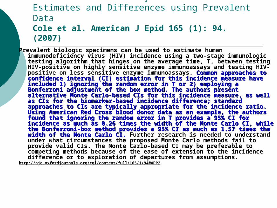
Confidence Intervals for Biomarker-based Human Immunodeficiency Virus Incidence Estimates and Differences using Prevalent DataCole et al. American J Epid 165 (1): 94. (2007)

Prevalent biologic specimens can be used to estimate human immunodeficiency virus (HIV) incidence using a two-stage immunologic testing algorithm that hinges on the average time, T, between testing HIV-positive on highly sensitive enzyme immunoassays and testing HIV-positive on less sensitive enzyme immunoassays. Common approaches Common approaches to confidence interval (CI) estimation for this incidence measure have to confidence interval (CI) estimation for this incidence measure have included 1) ignoring the random error in T or 2) employing a Bonferroni included 1) ignoring the random error in T or 2) employing a Bonferroni adjustment of the box method. The authors present alternative Monte adjustment of the box method. The authors present alternative Monte Carlo-based CIs for this incidence measure, as well as CIs for the Carlo-based CIs for this incidence measure, as well as CIs for the biomarker-based incidence difference; standard approaches to CIs are biomarker-based incidence difference; standard approaches to CIs are typically appropriate for the incidence ratio. Using American Red Cross typically appropriate for the incidence ratio. Using American Red Cross blood donor data as an example, the authors found that ignoring the blood donor data as an example, the authors found that ignoring the random error in T provides a 95% CI for incidence as much as 0.26 times random error in T provides a 95% CI for incidence as much as 0.26 times the width of the Monte Carlo CI, while the Bonferroni-box method the width of the Monte Carlo CI, while the Bonferroni-box method provides a 95% CI as much as 1.57 times the width of the Monte Carlo provides a 95% CI as much as 1.57 times the width of the Monte Carlo CI.CI. Further research is needed to understand under what circumstances the proposed Monte Carlo methods fail to provide valid CIs. The Monte Carlo-based CI may be preferable to competing methods because of the ease of extension to the incidence difference or to exploration of departures from assumptions.

http://aje.oxfordjournals.org/cgi/content/full/165/1/94#APP2

Your Turn to Try

Assess the Effect of Unequal Pop Variance in a 2-sample T-test

Design a MC study with to determine: What happens to the type I error rate? What happens to the Power?

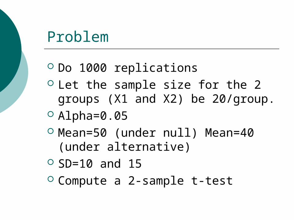
Problem

Do 1000 replications Let the sample size for the 2 groups

(X1 and X2) be 20/group. Alpha=0.05 Mean=50 (under null) Mean=40

(under alternative) SD=10 and 15 Compute a 2-sample t-test

Reference

SAS for Monte Carlo Studies: A Guide for Quantitative Researchers by Xitao Fan, Akos Felsovalyi, Stephen Sivo, and Sean Keenan Copyright(c) 2002 by SAS Institute Inc., Cary, NC, USA

ISBN 1-59047-141-5