Embed Size (px)
Citation preview
Computing Science Group
Nominal Game Semantics
Nikos Tzevelekos
CS-RR-09-18
Oxford University Computing Laboratory
Wolfson Building, Parks Road, Oxford, OX1 3QD
Nominal Game Semantics
Nikos Tzevelekos
Brasenose College
University of Oxford
Trinity 2008
A thesis submitted for the degree of Doctor of Philosophy

Abstract
Game Semantics arguably stands for one of the most successful techniques indenotational semantics, having provided not only proper denotational, accurate
models for a large variety of programming languages, but also new semantical
tools for program verification and validation. Most of all, over the last coupleof decades, game semantics has contributed a novel understanding of compu-
tations, namely as functions with inner structure, the latter being described asinteraction between two players— the Program and the Environment.
On the other hand, Nominal Computation is a key theme within the Theory of
Computation which has not been adressed semantically in a satisfactory man-
ner. The significance of nominal computation is clearly depicted in the ubiquityof names in computational scenarios: names form the basis of many calculi of
mobile processes; appear in network protocols and secure transactions; and aregenerally essential in programming for identifying variables, channels, threads,
objects, codes, and many other sorts of name in disguise.
This thesis examines nominal game semantics, that is, game semantics for nomi-nal computation. Our starting point is the basic nominal language, the ν-calculus,
which we model in a basic category of nominal games. The construction of nom-
inal games is based on recent advances in game semantics, and also on the the-ory of Nominal Sets, which serves as a general foundation for reasoning about
names.
Our main focus is on languages extending the basic nominal language by use ofnames for general references and exceptions. These languages faithfully reflect
the practice and reach the expressivity of programming languages such as ML;moreover, their full-abstraction problems had not been solved previously in a
fully satisfactory manner. Such solutions we provide herein. We first devise
abstract categorical models for these languages, and then construct fully abstractmodels in nominal games.
4
Preface to the Technical Report
This Report of December 2009 corrects discrepancies related to the terms M2
and M3 used in Chapters 4 and onwards (especially Section 5.2.6) in order to
distinguish the examined nominal calculi. I am grateful to Andrzej Murawskifor the many fruitful discussions, out of which those problems became apparent.
Acknowledgements
First, I would like to thank my supervisor, Samson Abramsky, for his constantencouragement, support and guidance, and his impeccable academic ethos. Fur-
thermore, certain people have been particularly supportive of this work, thusgreatly contributing to its successful completion; among them I would like to
single out Andy Pitts, Luke Ong, Andrzej Murawski, Guy McCusker, Dan Ghica
and Ian Stark. In addition, Andy was happy to offer advice on nominal matters;Guy readily advised on game-semantics; and Andrzej, Ian and Luke (the latter
two acting as examiners) read the thesis and suggested several corrections andimprovements. I would also like to thank Jim Laird, Paul Levy and Sam Sanjabi
for fruitful discussions, suggestions and criticisms.
Many thanks go to my friends during these years in Oxford, and particularly toElfy, Loukia, George, Nicholas, Antonis, Iris, Andria and Elina. I would also like
to thank my family for their faith and support. I am deeply grateful to Note, for
everything.
Finally, I would like to acknowledge the financial support of the Engineering andPhysical Sciences Research Council, the Eugenides Foundation, the A. G. Leven-
tis Foundation and Brasenose College.
Στη Νότα.
5
List of Figures
1.1 Cumulative Hierarchies in ZF and ZFA . . . . . . . . . . . . . . . . . . . . . . 11
2.1 Strong Support Lemma . . . . . . . . . . . . . . . . . . . . . . . . . . . . . . . . 212.2 The sν-calculus: typing and reduction rules. . . . . . . . . . . . . . . . . . . . 29
3.1 Basic arena constructions. . . . . . . . . . . . . . . . . . . . . . . . . . . . . . . 42
3.2 Definition of innocent play. . . . . . . . . . . . . . . . . . . . . . . . . . . . . . 54
4.1 The νρ-calculus: typing rules. . . . . . . . . . . . . . . . . . . . . . . . . . . . . 77
4.2 The νρ-calculus: reduction rules. . . . . . . . . . . . . . . . . . . . . . . . . . . 78
4.3 The semantic translation of νρ. . . . . . . . . . . . . . . . . . . . . . . . . . . . 834.4 The store arena ξ and the translation of νρ-types. . . . . . . . . . . . . . . . . . 91
4.5 The store monad (T, η, µ, τ) for νρ. . . . . . . . . . . . . . . . . . . . . . . . . . 924.6 The fresh-name natural transformation for νρ. . . . . . . . . . . . . . . . . . . 93
4.7 Update and dereferencing arrows in Vt. . . . . . . . . . . . . . . . . . . . . . . 94
4.8 A dialogue in innocent store. . . . . . . . . . . . . . . . . . . . . . . . . . . . . 964.9 Store-H’s -Q’s -A’s in arena T 1. . . . . . . . . . . . . . . . . . . . . . . . . . . . 101
5.1 Kleisli-composition for inner- and outer-component arrows. . . . . . . . . . . 1225.2 Equivalences separating our nominal calculi. . . . . . . . . . . . . . . . . . . . 127
5.3 The semantic translation of νερ-terms. . . . . . . . . . . . . . . . . . . . . . . . 128
5.4 The store arena ξ and the translation of νερ-types. . . . . . . . . . . . . . . . . 1325.5 The compound monad (T, η, µ, τ) for νερ. . . . . . . . . . . . . . . . . . . . . . 133
5.6 Natural transformations θ and nu for νερ. . . . . . . . . . . . . . . . . . . . . . 1345.7 Update and dereferencing arrows in Vt. . . . . . . . . . . . . . . . . . . . . . . 135
5.8 Exception-handling in Vt. . . . . . . . . . . . . . . . . . . . . . . . . . . . . . . 136
5.9 Store-H’s -Q’s -A’s and X-raisers in arena T 1. . . . . . . . . . . . . . . . . . . . 137
6

Contents
1 Introduction 9
1.1 Background Remarks . . . . . . . . . . . . . . . . . . . . . . . . . . . . . . . . . 10
1.1.1 Nominal Languages . . . . . . . . . . . . . . . . . . . . . . . . . . . . . 10
1.1.2 Nominal Sets . . . . . . . . . . . . . . . . . . . . . . . . . . . . . . . . . 101.1.3 Game Semantics . . . . . . . . . . . . . . . . . . . . . . . . . . . . . . . 11
1.2 Thesis Outline . . . . . . . . . . . . . . . . . . . . . . . . . . . . . . . . . . . . . 12
1.2.1 Main Contributions . . . . . . . . . . . . . . . . . . . . . . . . . . . . . . 13
2 Names, Nu and Monads 15
2.1 Nominal Sets . . . . . . . . . . . . . . . . . . . . . . . . . . . . . . . . . . . . . . 152.1.1 Definition . . . . . . . . . . . . . . . . . . . . . . . . . . . . . . . . . . . 15
2.1.2 Strong support . . . . . . . . . . . . . . . . . . . . . . . . . . . . . . . . 20
2.1.3 A historical note . . . . . . . . . . . . . . . . . . . . . . . . . . . . . . . 212.2 A paradigmatic nominal language . . . . . . . . . . . . . . . . . . . . . . . . . 24
2.2.1 The ν-calculus . . . . . . . . . . . . . . . . . . . . . . . . . . . . . . . . . 242.2.2 The sν-calculus . . . . . . . . . . . . . . . . . . . . . . . . . . . . . . . . 28
2.3 Monads and Comonads . . . . . . . . . . . . . . . . . . . . . . . . . . . . . . . 30
2.3.1 Monads . . . . . . . . . . . . . . . . . . . . . . . . . . . . . . . . . . . . 302.3.2 The Kleisli construction and the intrinsic preorder . . . . . . . . . . . . 31
2.3.3 Defining side-effects . . . . . . . . . . . . . . . . . . . . . . . . . . . . . 332.3.4 Monad composition . . . . . . . . . . . . . . . . . . . . . . . . . . . . . 34
2.3.5 Defining exceptions . . . . . . . . . . . . . . . . . . . . . . . . . . . . . 35
2.3.6 Comonads . . . . . . . . . . . . . . . . . . . . . . . . . . . . . . . . . . . 352.3.7 Monadic-comonadic setting . . . . . . . . . . . . . . . . . . . . . . . . . 37
3 Nominal Games 39
3.1 The basic category G of nominal games . . . . . . . . . . . . . . . . . . . . . . 40
3.1.1 Nominal arenas and strategies . . . . . . . . . . . . . . . . . . . . . . . 40
3.1.2 Composition . . . . . . . . . . . . . . . . . . . . . . . . . . . . . . . . . . 443.1.3 Arena and strategy orders in G . . . . . . . . . . . . . . . . . . . . . . . 52
3.2 Innocence . . . . . . . . . . . . . . . . . . . . . . . . . . . . . . . . . . . . . . . 53
3.2.1 The subcategory V . . . . . . . . . . . . . . . . . . . . . . . . . . . . . . 533.2.2 Viewfunctions . . . . . . . . . . . . . . . . . . . . . . . . . . . . . . . . . 58
3.2.3 Diagrams of viewfunctions . . . . . . . . . . . . . . . . . . . . . . . . . 603.3 Totality . . . . . . . . . . . . . . . . . . . . . . . . . . . . . . . . . . . . . . . . . 61
3.3.1 The subcategory Vt . . . . . . . . . . . . . . . . . . . . . . . . . . . . . . 61
3.3.2 Lifting and product . . . . . . . . . . . . . . . . . . . . . . . . . . . . . . 623.3.3 Partial exponentials . . . . . . . . . . . . . . . . . . . . . . . . . . . . . 65
3.3.4 Coproducts . . . . . . . . . . . . . . . . . . . . . . . . . . . . . . . . . . 673.3.5 Strategy and arena orders . . . . . . . . . . . . . . . . . . . . . . . . . . 68
3.4 A monad, and some comonads . . . . . . . . . . . . . . . . . . . . . . . . . . . 69
3.4.1 Lifting monad . . . . . . . . . . . . . . . . . . . . . . . . . . . . . . . . . 693.4.2 Initial-state comonads . . . . . . . . . . . . . . . . . . . . . . . . . . . . 70
7
8 CONTENTS
3.4.3 Fresh-name constructors . . . . . . . . . . . . . . . . . . . . . . . . . . . 713.5 Nominal games a la Laird . . . . . . . . . . . . . . . . . . . . . . . . . . . . . . 73
4 Nominal References 75
4.1 The νρ-calculus . . . . . . . . . . . . . . . . . . . . . . . . . . . . . . . . . . . . 76
4.2 Semantics . . . . . . . . . . . . . . . . . . . . . . . . . . . . . . . . . . . . . . . 80
4.2.1 Soundness . . . . . . . . . . . . . . . . . . . . . . . . . . . . . . . . . . . 814.2.2 Completeness . . . . . . . . . . . . . . . . . . . . . . . . . . . . . . . . . 85
4.3 The nominal games model . . . . . . . . . . . . . . . . . . . . . . . . . . . . . . 884.3.1 Solving the Store Equation . . . . . . . . . . . . . . . . . . . . . . . . . 88
4.3.2 The store monad T . . . . . . . . . . . . . . . . . . . . . . . . . . . . . . 91
4.3.3 Obtaining the νρ-model . . . . . . . . . . . . . . . . . . . . . . . . . . . 924.3.4 Adequacy . . . . . . . . . . . . . . . . . . . . . . . . . . . . . . . . . . . 96
4.3.5 Tidy strategies . . . . . . . . . . . . . . . . . . . . . . . . . . . . . . . . . 1004.3.6 Observationality . . . . . . . . . . . . . . . . . . . . . . . . . . . . . . . 107
4.3.7 Definability and full-abstraction . . . . . . . . . . . . . . . . . . . . . . 110
4.3.8 Equivalences established semantically . . . . . . . . . . . . . . . . . . . 117
5 Nominal Exceptions 119
5.1 The νε-calculus . . . . . . . . . . . . . . . . . . . . . . . . . . . . . . . . . . . . 119
5.1.1 Precompound monads . . . . . . . . . . . . . . . . . . . . . . . . . . . . 1215.1.2 Sound categorical semantics . . . . . . . . . . . . . . . . . . . . . . . . . 122
5.2 The νερ-calculus . . . . . . . . . . . . . . . . . . . . . . . . . . . . . . . . . . . . 1255.2.1 Categorical semantics . . . . . . . . . . . . . . . . . . . . . . . . . . . . 127
5.2.2 Full abstraction . . . . . . . . . . . . . . . . . . . . . . . . . . . . . . . . 130
5.2.3 The nominal games model . . . . . . . . . . . . . . . . . . . . . . . . . 1315.2.4 The sound model . . . . . . . . . . . . . . . . . . . . . . . . . . . . . . . 133
5.2.5 Full abstraction . . . . . . . . . . . . . . . . . . . . . . . . . . . . . . . . 1365.2.6 Equivalences established semantically . . . . . . . . . . . . . . . . . . . 143
6 Conclusion 145
A Deferred Proofs 147
Bibliography 151
Index 157
Chapter 1
Introduction
A focal point in Computer Science is the semantics of programs, i.e. What does a program re-ally mean? Afirst answer to the question is given bymeans of the machine code produced by
a compiler. However, this description is problematic if we are interested in a semantics in-
dependent of hardware and compiler design, revealing of the essence of computation hiddenbehind the implementation; a more abstract semantics is needed. In this direction, Opera-
tional Semantics considers programs as executing on an abstract, high-level computationalenvironment. The semantics of a program is then its observable behaviour in this environment.
Two programs are observationally equivalent if they have indistinguishable behaviours. This
procedural description of computation at a level of abstraction that is both useful and intu-itive is by and large thought of as giving the intended semantics of a programming language.
On the other hand, programs are expressive enough to be given a syntax-free descrip-
tion in an abstract mathematical domain. This method, calledDenotational Semantics, waspioneered by Strachey as a “mathematical semantics” of programming languages [Str66],
and was substantiated through the work of Scott on Domain Theory [Sco70]. With oper-ational semantics giving the intended program behaviour, a denotational model needs to
capture both the programming language and its observational equivalence. The model is
fully abstract if observational equivalence and denotational equality coincide through se-mantic translation.
The quest for fully abstract denotational semantics started with the purely functionallanguage PCF, introduced by Plotkin [Plo77] and embodying the logic LCF of Scott [Sco93].
With PCF it was understood that for full-abstraction it was necessary to work in a do-
main of ‘sequential’ functions: the parallel nature of argument evaluation inherent in or-dinary functions is simply impossible to capture with PCF. The problem was finally solved
in the mid 90’s independently by three teams of researchers: Abramsky, Jagadeesan andMalacaria [AJM00]; Hyland and Ong [HO00]; Nickau [Nic96]. Their models were based on
Game Semantics: computation was modelled by dynamic interaction between two partic-
ipants, one of them representing the program and the other the environment. It was soonrealised that the potential of game semantics was not confined to the semantics of PCF. The
flexibility in applying and removing conditions from the rules of the games, along withthe potentiality of altering the structure of the games themselves, allowed for the accurate
modelling of a wide range of programming languages exhibiting various computational ef-
fects. This series of full-abstraction results established gamemodels as a powerful paradigmwithin denotational semantics.
At around the same time that game semantics appeared on the scene, Pitts and Starkwere focusing on a computational effect pervasive in computing, the use of names, and
examined a prototypical nominal language, the ν-calculus [PS93]. Names are syntactic atoms
used to distinguish objects which are otherwise indistinguishable yet have distinct rolesinside a computation; more importantly, names can be dynamically generated provoking a
local-state effect. This latter feature along with mobility of names rendered the operational
semantics of this seemingly simple language quite intricate.
9
10 CHAPTER 1. INTRODUCTION
The full-abstraction problem for the ν-calculus remained open for a decade. Meanwhile,Gabbay and Pitts [GP02] had introduced Nominal Sets as a general mathematical foun-
dation for nominal structures, by revisiting the Fraenkel-Mostowski permutation modelsof ZFA discovered in the 20’s and 30’s. In 2004, Abramsky, Ghica, Murawski, Ong and
Stark [AGM+04], and independently Laird [Lai04], introduced Nominal Games for the se-
mantical description of nominal computation; [AGM+04] in particular proposed a fully ab-stract semantics for the ν-calculus. This thesis is a further investigation on nominal game
semantics. We rectify the discrepancies arising in the original presentation of [AGM+04]and then examine fully abstract semantics for languages with nominal general references
and nominal exceptions.
1.1 Background Remarks
1.1.1 Nominal Languages
One of the most pervasive features in computation is the use of names to distinguish entitiesthat are otherwise indistinguishable yet have distinct roles inside a computation. The names
we focus on have no inner structure whatsoever: in Needham’s taxonomy they correspond
to ‘pure names’ [Nee93]. Moreover, following theWhat’s newmotto of Pitts and Stark [PS93],names can be
created with local scope, compared for equality, and passed around via function applica-
tion.
The above describes the basic nominal specification, which we may refer to as the nomi-
nal effect. In programming languages, though, more specifications may be added so that
names be used for channels, threads, references, codes, exceptions, etc. We refer to such
languages generically as nominal languages. The prototypical nominal language is the ν-calculus [PS93], which constitutes a call-by-value λ-calculus incorporating the basic nom-
inal specification. Of the more sophisticated and more ‘realistic’ nominal languages, one
that stands out is the π-calculus of Milner [SW01]. It is the paradigmatic language incorpo-rating names-for-channels, providing a programming framework for concurrent processes
intercommunicating through named channels.Although constructed as simple computationally as possible, the ν-calculus exhibits a
rather delicate behaviour, [Sta97]:
Functions may have local names that remain private and persist from one use of the
function to the next; alternatively, names may be passed out of their original scope andcan even outlive their creator. It is precisely this mobility of names that allows the nu-
calculus to model issues of locality, privacy and non-interference.
Hence, this seemingly plain language became of increasing importance to semanticists. Re-search focused primarily on the notion of observational equivalence, which resisted all at-
tempts to be modelled accurately by use of ordinary (non-nominal) techniques, be they
denotational or operational [Sta94, Sta96, Sta97, ZN03].
1.1.2 Nominal Sets
Invented in the 20’s and 30’s by Fraenkel and Mostowski as a model of set theory with
atoms (ZFA), for showing its independence from the Axiom of Choice, nominal sets werere-introduced in the late 90’s by Gabbay and Pitts [GP02, Pit03] as a general framework for
the formal treatment of names and name-binding. Themain objective was to exploit the rich
structure of nominal sets for defining abstract syntaxes with variable binding which wouldincorporate ‘clean’ rules for structural recursion and induction. Nominal sets (and nominal
abstract syntax) have been used extensively for building languages with symbolic-binding
1.1. BACKGROUND REMARKS 11
constructors, for devising nominal theorem provers, and for studying programming lan-guage semantics: see [Che05] for a survey, and [Gab00, Che04, Shi05a] for thorough inves-
tigations.
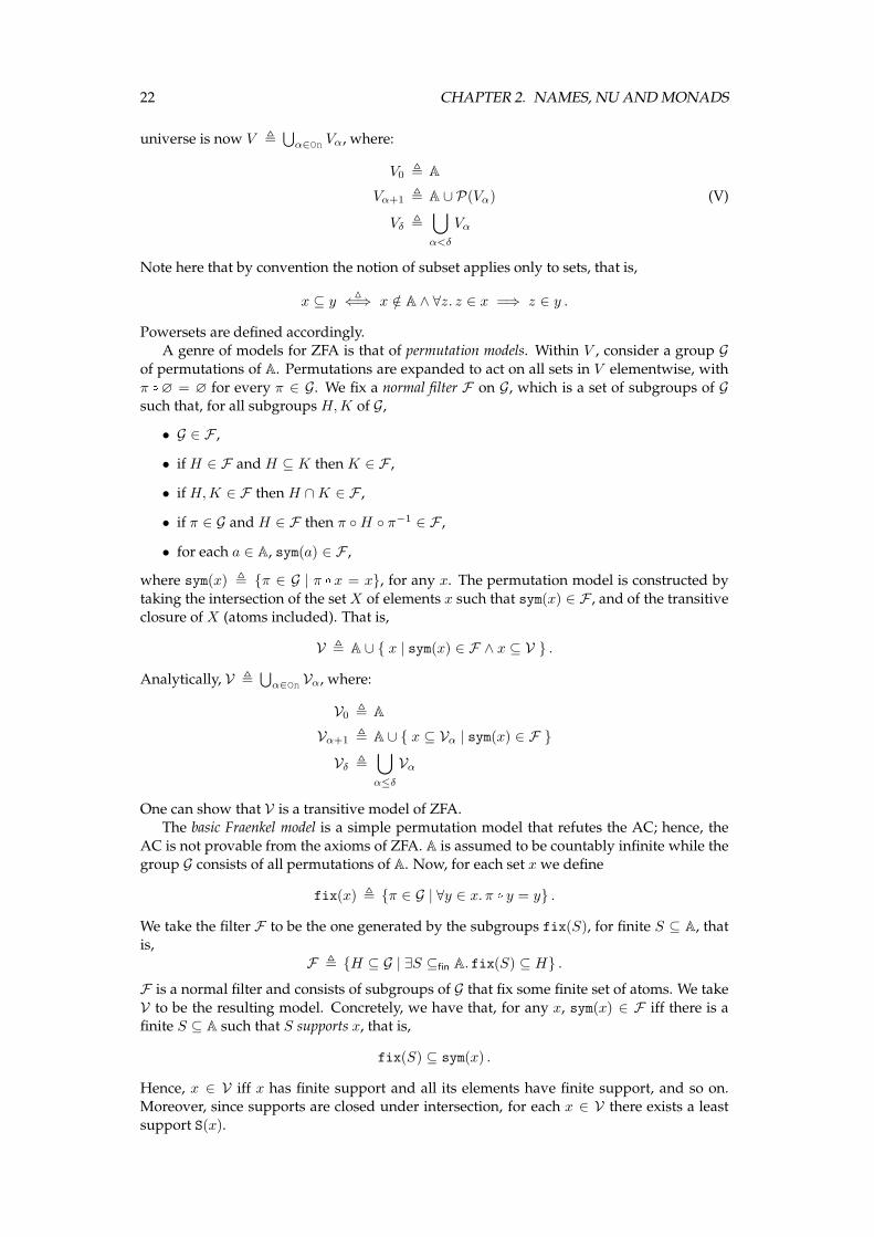
∅ A
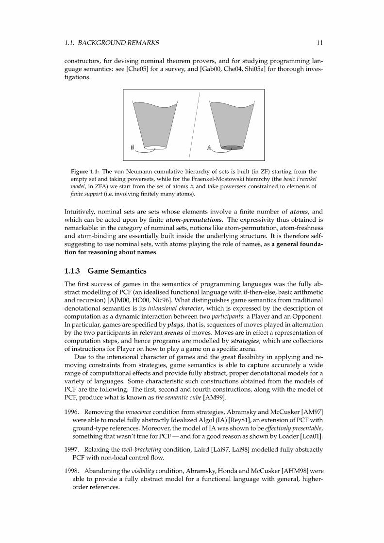
Figure 1.1: The von Neumann cumulative hierarchy of sets is built (in ZF) starting from the
empty set and taking powersets, while for the Fraenkel-Mostowski hierarchy (the basic Fraenkel
model, in ZFA) we start from the set of atoms A and take powersets constrained to elements of
finite support (i.e. involving finitely many atoms).
Intuitively, nominal sets are sets whose elements involve a finite number of atoms, andwhich can be acted upon by finite atom-permutations. The expressivity thus obtained is
remarkable: in the category of nominal sets, notions like atom-permutation, atom-freshnessand atom-binding are essentially built inside the underlying structure. It is therefore self-
suggesting to use nominal sets, with atoms playing the role of names, as a general founda-
tion for reasoning about names.
1.1.3 Game Semantics
The first success of games in the semantics of programming languages was the fully ab-
stract modelling of PCF (an idealised functional language with if-then-else, basic arithmeticand recursion) [AJM00, HO00, Nic96]. What distinguishes game semantics from traditional
denotational semantics is its intensional character, which is expressed by the description of
computation as a dynamic interaction between two participants: a Player and an Opponent.In particular, games are specified by plays, that is, sequences of moves played in alternation
by the two participants in relevant arenas of moves. Moves are in effect a representation of
computation steps, and hence programs are modelled by strategies, which are collectionsof instructions for Player on how to play a game on a specific arena.
Due to the intensional character of games and the great flexibility in applying and re-moving constraints from strategies, game semantics is able to capture accurately a wide
range of computational effects and provide fully abstract, proper denotational models for a
variety of languages. Some characteristic such constructions obtained from the models ofPCF are the following. The first, second and fourth constructions, along with the model of
PCF, produce what is known as the semantic cube [AM99].
1996. Removing the innocence condition from strategies, Abramsky and McCusker [AM97]
were able tomodel fully abstractly IdealizedAlgol (IA) [Rey81], an extension of PCFwith
ground-type references. Moreover, the model of IAwas shown to be effectively presentable,something that wasn’t true for PCF— and for a good reason as shown by Loader [Loa01].
1997. Relaxing the well-bracketing condition, Laird [Lai97, Lai98] modelled fully abstractly
PCF with non-local control flow.
1998. Abandoning the visibility condition, Abramsky, Honda andMcCusker [AHM98]wereable to provide a fully abstract model for a functional language with general, higher-
order references.

12 CHAPTER 1. INTRODUCTION
1999. Abandoning the determinacy condition, Harmer and McCusker [HM99, Har99] pro-duced a fully abstract model for finite-nondeterminism.
In addition to alterations to the constraints on strategies, variations to the notion of game
itself proved also meaningful computationally.
1996. Departing from the PCF models, McCusker [McC96, McC98] introduced a game-
setting with rich structure which allowed for the modelling of coproducts and the solu-
tion of domain equations on games. The result was a fully abstract model for FPC, anextension of PCF with coproducts and recursive types.
1997. Game models had thus far focused exclusively on call-by-name languages. At this
point, Honda and Yoshida [HY99] showed that the current framework of games could be
dualised appropriately, yielding the (equally primary) notion of call-by-value games. Atthe same time, Abramsky and McCusker [AM98] introduced a general categorical con-
struction, the family construction, which built CBV models from CBN ones, and applied
it to CBN games. The two constructions, which are essentially equivalent, yielded fullyabstract semantics for the CBV version of PCF.
1997. The introduction by Hughes of the notion of second-order move, that is, a move intro-
ducing a new ‘game-board’, lead to the development of hypergames and to full-abstraction
for system F [Hug97, Hug00].
The above results, which are by no means proposed as a complete enumeration of the
achievements of games, built a significant momentum for game semantics and established
it as a powerful paradigm in denotational semantics.
1.2 Thesis Outline
The thesis is structured as follows.
Chapter 2. In this chapter we present some background material necessary for the devel-
opments in the sequel. We start by presenting the theory of nominal sets, followingthe exposition of Pitts, and introducing the notion of strong support.
We continue by presenting the ν-calculus of Pitts and Stark, in a strongly supported
version, and give some of its basic properties.In the last partwe give an exposition of the categorical notions ofmonad and comonad,
and briefly examine the properties of monadic-comonadic (bi-Kleisli) categorical frame-
works.
Chapter 3. In this chapter we present (AGMOS-style) nominal games. These are ordinary,call-by-value, stateful games cast inside the universe of strong nominal sets. We in-
troduce the basic definitions of arenas, plays and strategies, and construct the basic
category of nominal games G. The rest of the chapter examines G and its subcategoriesV and Vt of innocent and total strategies respectively.
Chapter 4. This chapter introduces the νρ-calculus, an extension of the ν-calculuswith nom-
inal general references, and models it fully abstractly in nominal games. The seman-
tical part starts by presenting abstract categorical models, νρ-models, which give cor-rect interpretations of νρ. We then build a concrete such model in the category Vt,
and finally obtain full-abstraction by restricting to tidy strategies, that is, strategies
following a certain ‘discipline’ with regard to storage.
Chapter 5. In this chapter we examine fully abstract semantics for nominal exceptions in
nominal games. We introduce the calculi νε and νερ, which are extensions with nom-inal exceptions of the ν-calculus and the νρ-calculus respectively. Categorical models
for the calculi are presented: these are based on the fact that exceptions and local state
1.2. THESIS OUTLINE 13
are separable effects, described abstractly by the notion of precompound monad. Fi-nally, a specific fully abstract model for νερ is constructed in the subcategory of Vt
containing x-tidy strategies, that is, tidy strategies following some extra discipline forexceptions.
1.2.1 Main Contributions
The contributions of this thesis, which have also appeared in [Tze07, Tze08], can be sum-
marised as follows.
• The identification of strong nominal sets, that is, nominal sets with ‘ordered involvement’of names, as the appropriate setting for nominal languages and (mainly) their semantics.
• The abstract categorical description of the nominal effect of nominal languages. More-
over, the categorical presentation of fully abstract models of languages with nominal ref-erences and exceptions, in the spirit of [Abr00].
• The formulation/rectification of nominal games and their use in constructing models of
nominal references and exceptions.
• The introduction of game-disciplines to capture computation with names-as-references
and names-as-exceptions, leading to definable and hence fully abstract game models.
14 CHAPTER 1. INTRODUCTION
Chapter 2
Names, Nu and Monads
In this chapter we present background material necessary for this thesis. In section 2.1 wepresent the theory of Nominal Sets of Gabbay and Pitts, which we use as a general foun-
dation for constructions with names. In section 2.2 we present the basic nominal calculus,
i.e. the ν-calculus of Pitts and Stark, and also a version of the latter with ordered local state,the sν-calculus. In the final section we expose some results regarding the categorical notions
of monad and comonad.
2.1 Nominal Sets
The use of nominal sets in this thesis is limited, albeit essential. In particular, we express the
intuitive notion of names by use of atoms, either in the syntax of our languages or in theirdenotational semantics. The features of nominal sets allowing this modelling are:
• all finitely supported constructions with atoms can be carried out in nominal sets,
• atom-equality is decidable,
• there is an infinite supply of (fresh) atoms.
Another appealing feature of nominal sets is the ‘transparent’ notion of atom-permutation,
which we see as a ‘clean’ version of atom-substitution.Perhaps it is not clear to the reader why nominal sets should be used— couldn’t we sim-
ply model names by natural numbers? Indeed, numerals could be used for such semanticalpurposes (see e.g. [Lai08]), but they would constitute an over-specification: numerals carry
a linear order and a bottom element which would need to be carefully nullified in the se-
mantical definitions. Nominal sets factor out this burden by providing the minimal solutionto specifying names; in this sense, nominal sets are the intended model for names.
Finally, note that nominal sets appear in the literature also as “FM-sets” (e.g. [GP02]),since they descend from Fraenkel–Mostowski permutation models of set theory with atoms.
We will see more on that in section 2.1.3.
2.1.1 Definition
We are generally interested in languages having possibly infinitely many types of names,and hence we construct nominal sets over an ω-indexed family of sets of atoms. Thus, we
generally follow the presentation of [Pit03], the only difference being that, since we arenot interested in supplying “a first order theory of atoms and binding” (Nominal Logic),
we base our presentation on finite permutations instead of swappings of atoms (following
e.g. [PG00, Appendix]).Let us fix a countably infinite family (Ai)i∈ω of pairwise disjoint, countably infinite sets
of atoms, and let us denote by PERM(Ai) the group of finite permutations of Ai. Atoms
15
16 CHAPTER 2. NAMES, NU ANDMONADS
are denoted by a, b, c and variants; permutations are denoted by π and variants; id is theidentity permutation and (a b) is the permutation swapping a and b (and fixing all others).
We write A for the union of all the Ai’s. We take
PERM(A) ,⊕
i∈ω
PERM(Ai) (2.1)
to be the direct sum of the groups PERM(Ai), so PERM(A) is a group of finite permutations
of A which act separately on each constituent Ai. For each S ⊆ A we let
fix(S) , {π ∈ PERM(A) | ∀a∈S. π(a) = a} (2.2)
and say that a permutation π fixes S if π ∈ fix(S).
Recall that PERM(A) being a direct sum means that each π ∈ PERM(A) is an ω-indexed
list of permutations, π ∈∏
i∈ω PERM(Ai), and that (π)i 6= idAiholds for finitely many
indices i. If (π)i 6= idAiholds for exactly one index i then we call π a basic permutation, and
(π)i the basic component of π.
Fact 2.1 If π ∈ PERM(A) then,
• there exist basic permutations π1, ..., πn such that π = id ◦ π1 ◦ · · · ◦ πn ,
• there exist basic permutations π1, ..., πn such that the basic component of each πi is a
swapping, and π = id ◦ π1 ◦ · · · ◦ πn ,
• for any S ⊆ A, if π ∈ fix(S) then there exist basic permutations π1, ..., πn such that thebasic component of each πi is a swapping of atoms outside S, and π = id◦π1 ◦ · · ·◦πn.
We will therefore abandon the list-representation of permutations and—with a slight abuseof notation which identifies a basic permutation with its basic component—we will write
(non-uniquely) each permutation π as a finite composition π1 ◦ · · · ◦ πn such that each πibelongs to some PERM(Aj).
We proceed to nominal sets. As seen in the following definition, the notion of finite sup-
port is central to our presentation. More general supports have been examined in [Gab02,Che04]; in the latter work it is shown that the notion of support ideals completely corre-
sponds to the axioms of Nominal Logic. But these matters will not concern us here since all
our constructions entail finitely many atoms.
Definition 2.2 (Nominal Set on A) Anominal setX is a set |X | (usually denotedX) equipped
with an action of PERM(A), that is, a function [ : PERM(A)×X → X such that, for any
π, π′ ∈ PERM(A) and x ∈ X ,
π [(π′ [x) = (π ◦ π′) [x , id [x = x .
Moreover, for any x ∈ X there is a finite set S ⊆ A such that
fix(S) ⊆ {π ∈ PERM(A) | π [x = x} .
We say that S supports x. N
Concretely, a set S ⊆ A supports some x ∈ X if, for all permutations π,
(∀a∈S. π(a) = a) =⇒ π [x = x .
For example, A with the action of permutations being simply permutation-application is anominal set.
As shown below, finite support is closed under intersection. Hence, each element x of a
nominal set X has least finite support, called the support of x:
S(x) ,⋂
{S ⊆fin A | S supports x} . (2.3)
For example, for each atom a ∈ A, S(a) = {a}. We say that a is fresh for x, written a# x, if
a /∈ S(x). x is called equivariant if it has empty support.

2.1. NOMINAL SETS 17
Proposition 2.3 Let X be a nominal set and x ∈ X . For any finite S ⊆ A, S supports x iff
∀a, a′∈(A \ S). (a a′) [x = x .
Moreover, if finite S, S′ ⊆ A support x then S ∩ S′ also supports x. Finally,
S(x) = {a ∈ A | for infinitely many b. (a b) [x 6= x} .
Proof: For the first claim we need only show that S supports x if (a a′) [x = x for all atoms
a, a′ outside S. Assume the latter condition holds and take any π ∈ fix(S). By fact 2.1,π = id◦π1 ◦ · · · ◦πn with each πi being a swapping of atoms outside S, and hence π [x = x.
Now, if finite S, S′ ⊆ A support x then take any distinct a, a′ /∈ (S ∩ S′). For any b /∈S ∪ S′ ∪ {a, a′}, (a a′) [x = (a b) [(a′ b) [(a b) [x = x since (a b) [x = x = (a′ b) [x. Hence,
S ∩ S′ supports x.
Finally, letA , {a ∈ A | for infinitely many b. (a b) [x 6= x} .
If a ∈ A \ S(x) then there are infinitely many b such that (a b) [x 6= x and, since S(x) is finite,there is such a b /∈ S(x), as S(x) supports x. Hence, A ⊆ S(x). Conversely, it suffices to
show that (a a′) [x = x for all distinct a, a′ /∈ A. But a, a′ /∈ A implies that, for cofinitely
many b, (a b) [x = x = (a′ b) [x. Take some b 6= a, a′ of the cofinitely many; we have
(a a′) [x = (a b) [(a′ b) [(a b) [x = x .�
From the last part of the proposition we have:
a# x ⇐⇒ for cofinitely many b. (a b) [x = x
by defn⇐⇒ � b∈A. (a b) [x = x
(2.4)
The “fresh” quantifier � , introduced in [GP02], quantifies over cofinitely many atoms, i.e.�a∈A. φ(a)△
⇐⇒ for cofinitely many a∈A. φ(a) . (�)A subtlety here is that the holes in φ must all be of the same atom-type, say i, and that, in
fact, we mean “for cofinitely many a ∈ Ai”.
Example 2.4 There are several ways to obtain new nominal sets from given nominal sets X
and Y :
• The disjoint union X ⊎ Y with permutation-action inherited fromX and Y is a nominal
set. The construction easily extends to infinite disjoint union.
• The cartesian product X×Y with permutations acting componentwise is a nominal set;if (x, y) ∈ X×Y then S(x, y) = S(x) ∪ S(y).
• The fs-powerset Pfs(X), that is, the set of subsets of X which have finite support, with
permutations acting elementwise.
• X ′ ⊆ X is a nominal subset of X if X ′ is closed under permutations, these acting as onX .
• The fs-function spaceX→fsY , that is, the set of functions fromX to Y with finite support:
X →fs Y , {f ∈ Pfs(X×Y ) | f a function with domain X}.
Example 2.5 Apart from A, some standard nominal sets are the following.
18 CHAPTER 2. NAMES, NU ANDMONADS
• Using products and infinite unions we obtain the nominal set:
A# ,⋃
n∈ω
{ a1 . . . an | ∀i, j ∈ 1..n. ai ∈ A ∧ (i 6= j =⇒ ai 6= aj) } , (2.5)
that is, the set of finite lists of distinct atoms. Such lists we denote by~a,~b,~c and variants.For notational economy, we write a ∈ ~a for a ∈ S(~a). Moreover, for each ~a ∈ A# we set:
A~a , { π [~a | π ∈ PERM(A) } . (2.6)
Finally, for ~a,~b ∈ A# we write:
• ~a ≤ ~b if ~a is a prefix of~b,
• ~a � ~b if ~a is a (not necessarily contiguous) sublist of~b,
• ~a ⊆ ~b if S(~a) ⊆ S(~b).
• The fs-powerset Pfs(A) is the set of finite and cofinite sets of atoms, and has Pfin(A) as a
nominal subset (the set of finite sets of atoms).
ForX and Y nominal sets, a relationR ⊆ X×Y is a nominal relation if it is a nominal subsetof X×Y . Concretely,R is a nominal relation iff, for any permutation π and (x, y) ∈ X×Y ,
xRy ⇐⇒ (π [x)R(π [ y) . (2.7)
For example, # ⊆ A×X is a nominal relation: for all relevant a, x, π,
a# x =⇒ � b∈A. (a b) [x = x =⇒ � b∈A. π [(a b) [x = π [x=⇒ � b∈A. (π(a) π(b)) [π [x = π [x =⇒ � b′∈A. (π(a) b′) [π [x = π [x=⇒ π(a) # π [x .
From nominal relations we proceed to nominal functions and the category of nominal sets.
Definition 2.6 (The category Nom) A function f : X → Y is a nominal function if, for any
π ∈ PERM(A) and x ∈ X ,f(π [x) = π [ f(x) .
We let Nom be the category of nominal sets and nominal functions. N
Thus, nominal functions are fs-functions with empty support. For example, the supportfunction S( ) : XB Pfin(A) is a nominal function since S(π [x) = π [ S(x).
Nom inherits rich structure from Set and is in particular a topos. More importantly,
it contains atom-abstraction mechanisms. The mechanism which triggered the study ofnominal sets in programming is the following. For any nominal set X , any x ∈ X and any
a ∈ A, we can abstract a from x by forming
〈a〉x , {(b, y) ∈ A×X | (b = a ∨ b# x) ∧ y = (a b) [x} .The abstraction takes the orbit of (a, x) under all swappings of a for fresh atoms. In λ-calculus terminology, 〈a〉x is literally the α-equivalence class of (a, x) (that is, with regard
to the abstraction of a). Hence, it is not difficult to see that S(〈a〉x) = S(x) \ {a}. Moreover,π [〈a〉x = 〈π [a〉(π [x) and therefore we can define the nominal set 〈A〉X ⊆ Pfs(A×X) of
abstracted elements as
〈A〉X , {〈a〉x | a ∈ A ∧ x ∈ X} ,
and atom-abstraction as an arrow 〈 〉 : A×XB 〈A〉X in Nom.However, in this thesis we are not interested in treating name- and variable-abstractions
nominally, and therefore we will not use the above form of abstraction. The abstraction
mechanism which is useful to us, instead of abstracting specified atoms from x, abstracts allatoms outside a specified subset of S(x). It is therefore similar to the abstaction mechanisms
used in [AGM+04, Tze07].
2.1. NOMINAL SETS 19
Definition 2.7 (Support abstraction) Let X be a nominal set and x ∈ X . For any finiteS ⊆ A, we can abstract x to S, by forming
[x]S , {y ∈ X | ∃π∈fix(S ∩ S(x)). y = π [x} .N
This form of abstraction restricts the support of x to S ∩ S(x) by appropriate orbiting of x(and note that [x]S ∈ Pfs(X)). This is shown in the following lemma, along with the fact that
[ ] is itself nominal.
Lemma 2.8 For any x ∈ X , S ⊆fin A and π ∈ PERM(A),
• π [[x]S = [π [x]π [S ,• S([x]S) = S(x) ∩ S .
Proof: For the first clause, we have:
y ∈ π [[x]S ∃π′
=⇒ y = π [π′ [x ∧ ∀a∈S ∩ S(x). π′ [a = a
=⇒ y = (π ◦ π′ ◦ π−1) [π [x ∧ ∀a∈S ∩ S(x). (π ◦ π′ ◦ π−1) [π [ a = π [a=⇒ y = (π ◦ π′ ◦ π−1) [π [x ∧ ∀a′∈π [(S ∩ S(x)). (π ◦ π′ ◦ π−1) [ a′ = a′
=⇒ y ∈ [π [x]π [S (note π [(S ∩ S(x)) = (π [S) ∩ S(π [x) ) ,
z ∈ [π [x]π [S ∃π′
=⇒ z = π′ [π [x ∧ ∀a′∈π [(S ∩ S(x)). π′ [a′ = a′
=⇒ z = π′ [π [x ∧ ∀a∈S ∩ S(x). π′ [π [a = π [a=⇒ z = π [(π−1 ◦ π′ ◦ π) [x ∧ ∀a∈S ∩ S(x). (π−1 ◦ π′ ◦ π) [ a = π−1 [π [ a = a
=⇒ z ∈ π [[x]S .Note that ∀π. π [[x]S = [π [x]π [S implies S([x]S) ⊆ S(x) ∪ S.For the second clause, assume a ∈ S ∩ S(x) and a# [x]S . Then, for any b#x, S, (a b) [[x]S =
[x]S , and hence x ∈ (a b) [[x]S . This means there exists π ∈ fix(S ∩ S(x)) such that x =
(a b) [π [x, and therefore a ∈ S(x) implies
b = (a b) [π [a ∈ S((a b) [π [x) = S(x) ,to b# x. Hence, S ∩ S(x) ⊆ S([x]S).For the converse, for any a, b /∈ S ∩ S(x), we have
(a b) [[x]S = {(a b) [π [x | π ∈ fix(S ∩ S(x))} = {π [x | π ∈ fix(S ∩ S(x))} = [x]S ,
and hence S([x]S) ⊆ S ∩ S(x). �
Two particular subcases of support abstraction are of interest. First, in case S ⊆ S(x), theabstraction becomes
[x]S = {y ∈ X | ∃π∈fix(S). y = π [x} . (∗)
This is the mechanism used in [Tze07].1 Note that if S * S(x) ∧ S(x) * S then (∗) does notyield S([x]S) = S ∩ S(x). Note also (proof left as exercise) that if S ⊆ S(x) ∩ S(y) then
[x]S = [y]S ⇐⇒ y ∈ [x]S . (2.8)
The other subcase is the simplest possible, that is, of S being empty; it turns out that this is
all we need from support abstractions in this thesis. We define:
[x] , {y ∈ X | ∃π. y = π [x} . (2.9)
1The mechanism used in [AGM+04] is [x]S , {(y, S) | ∃π∈fix(S). y = π [ x} , and is equivalent to the othertwo in case S ⊆ S(x), but not in general.
20 CHAPTER 2. NAMES, NU ANDMONADS
2.1.2 Strong support
Nominal sets describe a framework of objects built around a finite (or cofinite) amount ofatoms. The framework does not specify how these atoms are present inside an object’s
structure, so atoms may appear in an ‘unordered’ fashion, as for example in the set {a, b}.The distinction between ordered and unordered involvement of atoms can be formally seen
in the definition of support. In particular, we have seen that a set S supports x if
(∀a∈S. π(a) = a) =⇒ π [x = x .
Ordered involvement then means that the reverse implication is also true. This notion we
call strong support.
Definition 2.9 For any nominal set X , any x ∈ X and any S ⊆ A, S strongly supports x if
fix(S) = { π ∈ PERM(A) | π [x = x } .
We say thatX is a strong nominal set if all its elements have strong support. N
Thus, the set {a, b} does not support {a, b} strongly, since the permutation (a b) does not fix{a, b},2 but still (a b) [{a, b} = {a, b}. On the other hand, {a, b} strongly supports the list ab.
In fact, all finite lists of (distinct) atoms have strong support, and therefore A# is a strongnominal set.
The notion of strong support is stronger than that of support, as we saw in the example
of {a, b}. Nonetheless, strong support coincides with weak support when the former exists.
Proposition 2.10 IfX is a nominal set and x ∈ X has strong support S then S = S(x).
Proof: By definition, S supports x, so S(x) ⊆ S. Now suppose there exists a ∈ S \ S(x). Forany fresh b, (a b) fixes S(x) but not S, so it doesn’t fix x, . �
Hence, Pfin(A) is not a strong nominal set (but A# is). The main reason for using strongnominal sets is the following result.
Lemma 2.11 (Strong support lemma) Let X be a strong nominal set and x1, x2, y1, y2, z1, z2 ∈X . Suppose also that, for some S ⊆fin A,
S ⊆ S(zi) ∩ S(yi) ⊆ S(xi) ,
for i = 1, 2, and there exist πy, πz ∈ fix(S) such that
πy [x1 = πz [x1 = x2 , πy [ y1 = y2 , πz [ z1 = z2 .
Then, there exists some π ∈ fix(S) such that π [x1 = x2 , π [ y1 = y2 and π [ z1 = z2.
Proof: Note that S(zi) ∩ S(yi) ⊆ S(xi) iff (S(zi) \ S(xi)) ∩ S(yi) = ∅. Let ∆i , S(zi) \ S(xi) ,i = 1, 2 , so ∆2 = πz [∆1, and let π′ , π−1
y ◦ πz . By assumption, π′ [x1 = x1, and thereforeπ′ ∈ fix(S(x1)) by strong support. Take any b ∈ ∆1. Then, π′(b) # π′ [x1 = x1 and
πz(b) ∈ πz [∆1 = ∆2, ∴ πz(b) # y2, ∴ π′(b) # π−1y [ y2 = y1. Hence,
b ∈ ∆1 =⇒ b, π′(b) # x1, y1 .
Now assume ∆1 = {b1, ..., bN} and define π0, π1, ..., πN by recursion:
π0 , id , πi+1 , (bi+1 (πi ◦ π′)(bi+1)) ◦ πi .
We claim that, for each 0 ≤ i ≤ N and 1 ≤ j ≤ i, we have
πi [π′ [ bj = bj , πi [x1 = x1 , πi [ y1 = y1 .
2Recall that a permutation π fixes a set of atoms S if π(a) = a for all a ∈ S.
2.1. NOMINAL SETS 21
We do induction on i; the case of i = 0 is trivial. For the inductive step, if πi [π′ [ bi+1 = bi+1
then πi+1 = πi, and πi+1 [π′ [ bi+1 = πi [π′ [ bi+1 = bi+1. Moreover, by IH, πi+1 [π′ [ bj =
bj for all 1 ≤ j ≤ i, and πi+1 [x1 = x1 and πi+1 [ y1 = y1. If πi [π′ [ bi+1 = b′i+1 6= bi+1 then,by construction, πi+1 [π′ [ bi+1 = bi+1. Moreover, for each 1 ≤ j ≤ i, by IH, πi+1 [π′ [ bj =
(bi+1 b′i+1) [ bj , and the latter equals bj since bi+1 6= bj implies b′i+1 6= πi [π′ [ bj = bj . Finally,
for any a ∈ S(x1)∪S(y1), πi+1 [ a = (bi+1 b′i+1) [πi [a = (bi+1 b
′i+1) [a, by IH, with a 6= bi+1.
But the latter equals a since π′(bi+1) 6= a implies that b′i+1 6= πi [a = a, as required.
Hence, for each 1 ≤ j ≤ N ,
πN [π′ [ bj = bj , πN [x1 = x1 , πN [ y1 = y1 .
Moreover, πN [π′ [ z1 = z1, as we also have
b ∈ S(z1) ∩ S(x1) =⇒ πN [π′ [ b = πN [ b = b
(again by strong support). Thus, taking π , πy ◦ π−1N we have:
πy [π−1N [x1 = πy [x1 = x2 , πy [π−1
N [ y1 = πy [ y1 = y2 ,
πy [π−1N [ z1 = πy [π−1
N [πN [π′ [ z1 = πy [π′ [ z1 = πy [π−1y [πz [ z1 = z2 .
Finally, from πN ∈ fix(S(x1)) ⊆ fix(S) and πy ∈ fix(S) we obtain π ∈ fix(S). �
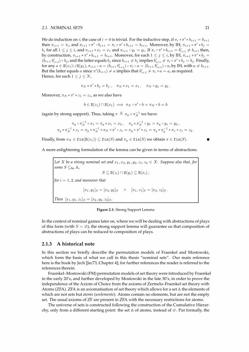
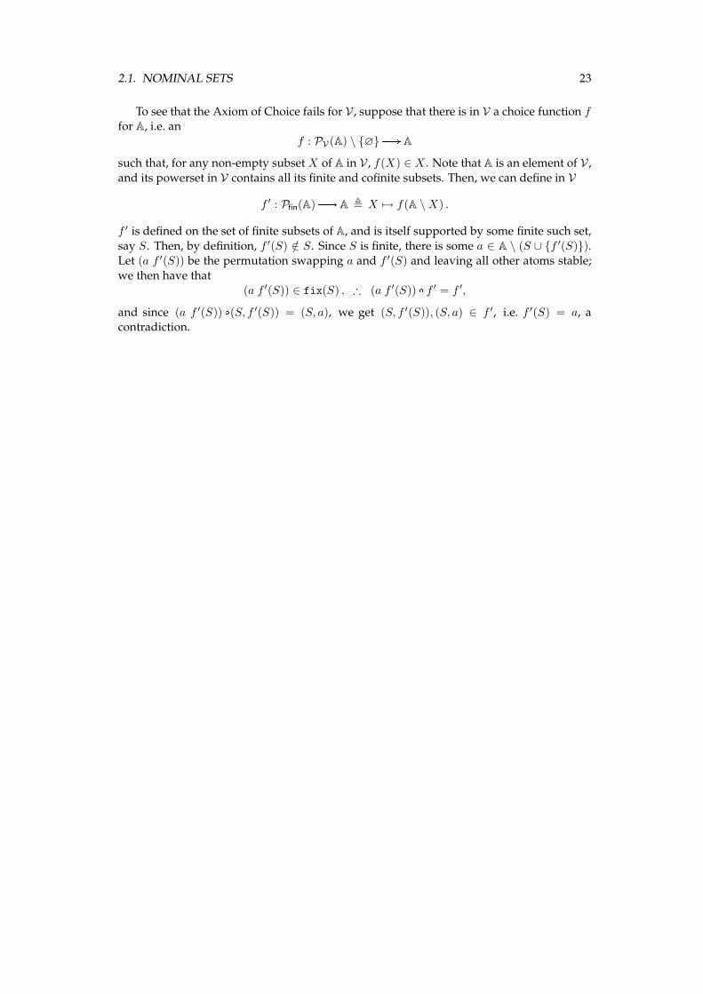
A more enlightening formulation of the lemma can be given in terms of abstractions.
Let X be a strong nominal set and x1, x2, y1, y2, z1, z2 ∈ X . Suppose also that, for
some S ⊆fin A,
S ⊆ S(zi) ∩ S(yi) ⊆ S(xi) ,
for i = 1, 2, and moreover that
[x1, y1]S = [x2, y2]S ∧ [x1, z1]S = [x2, z2]S .
Then [x1, y1, z1]S = [x2, y2, z2]S .
Figure 2.1: Strong Support Lemma
In the context of nominal games later on, wherewewill be dealingwith abstractions of playsof this form (with S = ∅), the strong support lemma will guarantee us that composition of
abstractions of plays can be reduced to composition of plays.
2.1.3 A historical note
In this section we briefly describe the permutation models of Fraenkel and Mostowski,
which form the basis of what we call in this thesis “nominal sets”. Our main reference
here is the book by Jech [Jec73, Chapter 4]; for further references the reader is referred to thereferences therein.
Fraenkel–Mostowski (FM) permutationmodels of set theorywere introduced by Fraenkel
in the early 20’s, and further developed by Mostowski in the late 30’s, in order to prove theindependence of the Axiom of Choice from the axioms of Zermelo–Fraenkel set theory with
Atoms (ZFA). ZFA is an axiomatisation of set theory which allows for a set A the elements ofwhich are not sets but atoms (urelemente). Atoms contain no elements, but are not the empty
set. The usual axioms of ZF are present in ZFA with the necessary restrictions for atoms.
The universe of sets is constructed following the construction of the Cumulative Hierar-chy, only from a different starting point: the set A of atoms, instead of ∅. Put formally, the
22 CHAPTER 2. NAMES, NU ANDMONADS
universe is now V ,⋃
α∈On Vα, where:
V0 , A
Vα+1 , A ∪ P(Vα) (V)
Vδ ,⋃
α<δ
Vα
Note here that by convention the notion of subset applies only to sets, that is,
x ⊆ y△
⇐⇒ x /∈ A ∧ ∀z. z ∈ x =⇒ z ∈ y .
Powersets are defined accordingly.A genre of models for ZFA is that of permutation models. Within V , consider a group G
of permutations of A. Permutations are expanded to act on all sets in V elementwise, with
π [∅ = ∅ for every π ∈ G. We fix a normal filter F on G, which is a set of subgroups of Gsuch that, for all subgroups H,K of G,
• G ∈ F ,
• ifH ∈ F and H ⊆ K thenK ∈ F ,
• ifH,K ∈ F thenH ∩K ∈ F ,
• if π ∈ G and H ∈ F then π ◦H ◦ π−1 ∈ F ,
• for each a ∈ A, sym(a) ∈ F ,
where sym(x) , {π ∈ G | π [x = x}, for any x. The permutation model is constructed by
taking the intersection of the setX of elements x such that sym(x) ∈ F , and of the transitiveclosure ofX (atoms included). That is,
V , A ∪ { x | sym(x) ∈ F ∧ x ⊆ V } .
Analytically, V ,⋃
α∈On Vα, where:
V0 , A
Vα+1 , A ∪ { x ⊆ Vα | sym(x) ∈ F }
Vδ ,⋃
α≤δ
Vα
One can show that V is a transitive model of ZFA.The basic Fraenkel model is a simple permutation model that refutes the AC; hence, the
AC is not provable from the axioms of ZFA. A is assumed to be countably infinite while thegroup G consists of all permutations of A. Now, for each set xwe define
fix(x) , {π ∈ G | ∀y ∈ x. π [ y = y} .
We take the filter F to be the one generated by the subgroups fix(S), for finite S ⊆ A, thatis,
F , {H ⊆ G | ∃S ⊆fin A. fix(S) ⊆ H} .
F is a normal filter and consists of subgroups of G that fix some finite set of atoms. We take
V to be the resulting model. Concretely, we have that, for any x, sym(x) ∈ F iff there is afinite S ⊆ A such that S supports x, that is,
fix(S) ⊆ sym(x) .
Hence, x ∈ V iff x has finite support and all its elements have finite support, and so on.Moreover, since supports are closed under intersection, for each x ∈ V there exists a least
support S(x).
2.1. NOMINAL SETS 23
To see that the Axiom of Choice fails for V , suppose that there is in V a choice function ffor A, i.e. an
f : PV(A) \ {∅}B A
such that, for any non-empty subset X of A in V , f(X) ∈ X . Note that A is an element of V ,and its powerset in V contains all its finite and cofinite subsets. Then, we can define in V
f ′ : Pfin(A) B A , X 7→ f(A \X) .
f ′ is defined on the set of finite subsets of A, and is itself supported by some finite such set,
say S. Then, by definition, f ′(S) /∈ S. Since S is finite, there is some a ∈ A \ (S ∪ {f ′(S)}).Let (a f ′(S)) be the permutation swapping a and f ′(S) and leaving all other atoms stable;
we then have that(a f ′(S)) ∈ fix(S) , ∴ (a f ′(S)) [ f ′ = f ′,
and since (a f ′(S)) [(S, f ′(S)) = (S, a), we get (S, f ′(S)), (S, a) ∈ f ′, i.e. f ′(S) = a, acontradiction.
24 CHAPTER 2. NAMES, NU ANDMONADS
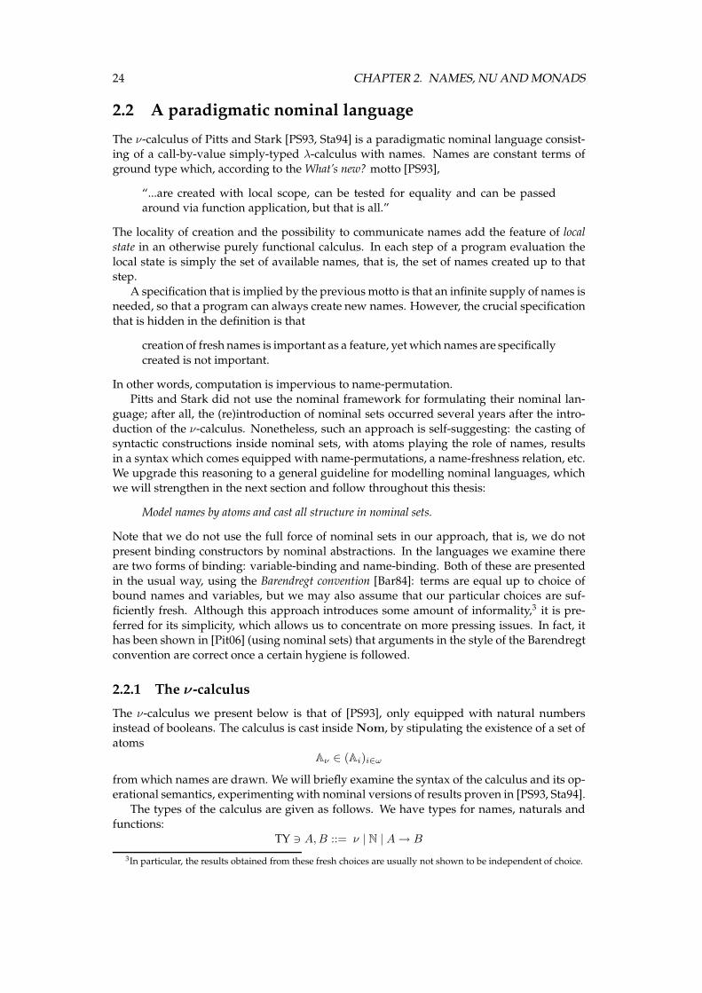
2.2 A paradigmatic nominal language
The ν-calculus of Pitts and Stark [PS93, Sta94] is a paradigmatic nominal language consist-ing of a call-by-value simply-typed λ-calculus with names. Names are constant terms of
ground type which, according to the What’s new? motto [PS93],
“...are created with local scope, can be tested for equality and can be passedaround via function application, but that is all.”
The locality of creation and the possibility to communicate names add the feature of local
state in an otherwise purely functional calculus. In each step of a program evaluation the
local state is simply the set of available names, that is, the set of names created up to thatstep.
A specification that is implied by the previousmotto is that an infinite supply of names isneeded, so that a program can always create new names. However, the crucial specification
that is hidden in the definition is that
creation of fresh names is important as a feature, yet which names are specifically
created is not important.
In other words, computation is impervious to name-permutation.Pitts and Stark did not use the nominal framework for formulating their nominal lan-
guage; after all, the (re)introduction of nominal sets occurred several years after the intro-
duction of the ν-calculus. Nonetheless, such an approach is self-suggesting: the casting ofsyntactic constructions inside nominal sets, with atoms playing the role of names, results
in a syntax which comes equipped with name-permutations, a name-freshness relation, etc.We upgrade this reasoning to a general guideline for modelling nominal languages, which
we will strengthen in the next section and follow throughout this thesis:
Model names by atoms and cast all structure in nominal sets.
Note that we do not use the full force of nominal sets in our approach, that is, we do not
present binding constructors by nominal abstractions. In the languages we examine thereare two forms of binding: variable-binding and name-binding. Both of these are presented
in the usual way, using the Barendregt convention [Bar84]: terms are equal up to choice ofbound names and variables, but we may also assume that our particular choices are suf-
ficiently fresh. Although this approach introduces some amount of informality,3 it is pre-
ferred for its simplicity, which allows us to concentrate on more pressing issues. In fact, ithas been shown in [Pit06] (using nominal sets) that arguments in the style of the Barendregt
convention are correct once a certain hygiene is followed.
2.2.1 The ν-calculus
The ν-calculus we present below is that of [PS93], only equipped with natural numbersinstead of booleans. The calculus is cast inside Nom, by stipulating the existence of a set of
atomsAν ∈ (Ai)i∈ω
fromwhich names are drawn. We will briefly examine the syntax of the calculus and its op-erational semantics, experimenting with nominal versions of results proven in [PS93, Sta94].
The types of the calculus are given as follows. We have types for names, naturals and
functions:TY ∋ A,B ::= ν | N | A→ B
3In particular, the results obtained from these fresh choices are usually not shown to be independent of choice.

2.2. A PARADIGMATIC NOMINAL LANGUAGE 25
Terms form a strong nominal set TE:
TE ∋M,N ::= x | λx.M |M N λ-calculus
| n | predM | succN arithmetic
| if0M thenN1 elseN2 if then else
| a name, a ∈ Aν
| [M = N ] name-equality test
| νa.M ν-abstraction
Of the terms above, the values are:
VA ∋ V,W ::= n | a | x | λx.M
Permutations act on TE componentwise, that is, for any π ∈ PERM(A),
π [ a = π(a) π [ νa.M = ν(π [a).(π [M) π [x = x π [λx.M = λx.(π [M) etc.
Note that there are two types of binding in the syntax, variable-binding and name-binding,
and each of these yields its own notion of α-equivalence (note also that variables are notnames). The set of free variables of a term is defined by:
fv(x) , {x} , fv(λx.M) , fv(M) \ {x} , fv(νa.M) , fv(M) , fv(n) = fv(a) , ∅ ,
plus standard rules for the other non-binding constructs. A term M is closed if fv(M) is
empty. Similarly, the set of free names of a term is defined by:
fn(a) , {a} , fn(νa.M) , fn(M) \ {a} , fn(λx.M) , fn(M) , fn(n) = fn(x) , ∅ ,
plus standard rules for the other non-binding constructs. α-equivalence for variable-binding,
henceforth called αV -equivalence and written =αV, is defined as usually.4α-equivalence for
name-binding, henceforth called αN -equivalence and written =αN, is defined by recursion
(on term size) as follows,
M = x, a, nM =αN
M
� b∈Aν . (a b) [M =αN(a′ b) [M ′
νa.M =αNνa′.M ′
M =αNM ′
λx.M =αNλx.M ′
plus standard rules for the other non-binding constructs. The definition is adapted from [GP02]
and it captures the usual notion of α-equivalence, i.e. it equates terms up to choice of boundnames (v. [GP02, proposition 2.2]).
The casting of our calculus in nominal sets equips us with a well-behaved action ofname-permutation and a crisp notion of name-freshness. In the following proposition we
give a couple of examples of results that can be shown with elegance using these mecha-
nisms. Note that a consequence of the first result is that the second rule for =αNreduces to
M =αNM ′
νa.M =αNνa.M ′
for a = a′.
Proposition 2.12 For all termsM,N and a, b ∈ Aν ,
• M =αNN =⇒ (a b) [M =αN
(a b) [N ,
• a, b /∈ fn(M) =⇒ (a b) [M =αNM .
Proof: The first claim is shown by induction on M , and the only non-trivial case is that
of ν-abstraction. So let M = νa′.M ′ and M =αNN . By definition, N = νb′.N ′ and� c. (a′ c) [M ′ =αN
(b′ c) [N ′. For any such c#a, b, by IH, (a b) [(a′ c) [M ′ =αN(a b) [(b′ c) [N ′.
Taking a′′ = (a b) [a′ and b′′ = (a b) [ b′ we have (a′′ c) [(a b) [M ′ =αN(b′′ c) [(a b) [N ′,
4i.e. nominally! See [Kri90].
26 CHAPTER 2. NAMES, NU ANDMONADS
and therefore νa′′.(a b) [M ′ =αNνb′′.(a b) [N ′, as required.
For the second claim we do induction on M and assume a 6= b. Again, the only non-
trivial case is that of ν-abstraction, so let M = νa′.M ′. If a′ # a, b, then (a b) [M =
νa′.(a b) [M ′ and a, b /∈ fn(M ′) so, by IH, (a b) [M ′ =αNM ′ and therefore, by use of first
claim, νa′.(a b) [M ′ =αNνa′.M ′. If a′ ∈ {a, b}, say a′ = a, then (a b) [M = νb.(a b) [M ′
and b /∈ fn(M ′) so, by IH and for any fresh c, (b c) [M ′ =αNM ′, hence, by first claim,
(b c) [(a b) [M ′ = (a c) [(b c) [M ′ =αN(a c) [M ′, and therefore νb.(a b) [M ′ =αN
νa.M ′, as
required. �
We now take the usual step of equating terms up to α-equivalence. It is true that the nominal
setting allows us to work without αN -equivalence with relevant elegance, but such a choicewould undeservedly complicate our presentation.
We assume the set of terms is quotiented by α-equivalence for both binding mechanisms,
that is, we equate terms up to choice of bound variables and bound names.
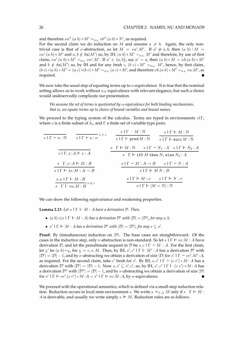
We proceed to the typing system of the calculus. Terms are typed in environments s^Γ,where s is a finite subset of Aν and Γ a finite set of variable-type pairs.
s ^ Γ_ n : Na ∈ s
s ^ Γ_ a : ν
s ^ Γ_M : N
s ^ Γ_ predM : N
s ^ Γ_M : N
s ^ Γ_ succM : N
s ^ Γ, x :A_ x : A
s ^ Γ_M : N s ^ Γ_N1 : A s ^ Γ_N2 : A
s ^ Γ_ if0M thenN1 elseN2 : A
s ^ Γ, x :A_M : B
s ^ Γ_ λx.M : A→ B
s ^ Γ_M : A→ B s ^ Γ_N : A
s ^ Γ_M N : B
s, a ^ Γ_M : Ba /∈ s
s ^ Γ_ νa.M : B
s ^ Γ_M : ν s ^ Γ_N : ν
s ^ Γ_ [M = N ] : N
We can show the following equivariance and weakening properties.
Lemma 2.13 Let s ^ Γ_M : A have a derivation D. Then,
• (a b) [(s ^ Γ_M : A) has a derivation D′ with |D| = |D′|, for any a, b,
• s′ ^ Γ_M : A has a derivation D′ with |D| = |D′|, for any s ⊆ s′.
Proof: By (simultaneous) induction on |D|. The base cases are straightforward. Of thecases in the inductive step, only ν-abstraction is non-standard. So let s ^ Γ_ νc.M : A have
derivation D, and let the penultimate sequent in D be s, c ^ Γ_M : A. For the first claim,
let χ′ be (a b) [χ, for χ = c, s,M . Then, by IH, s′, c′ ^ Γ_M ′ :A has a derivation D′ with|D′| = |D| − 1, and by ν-abstracting we obtain a derivation of size |D| for s′ ^ Γ_ νc′.M ′ :A,
as required. For the second claim, take c′ fresh for s′. By IH, s, c′ ^ Γ_ (c c′) [M :A has aderivation D′ with |D′| = |D| − 1. Now s, c′ ⊆ s′, c′, so, by IH, s′, c′ ^ Γ_ (c c′) [M :A has
a derivation D′′ with |D′′| = |D| − 1, and by ν-abstracting we obtain a derivation of size |D|for s′ ^ Γ_ νc′.(c c′) [M :A = s′ ^ Γ_ νc.M :A, by α-equivalence. �
We proceedwith the operational semantics, which is defined via a small-step reduction rela-tion. Reduction occurs in local state environment s. We write s`Γ,A M only if s ^ Γ_M :
A is derivable, and usually we write simply s`M . Reduction rules are as follows.
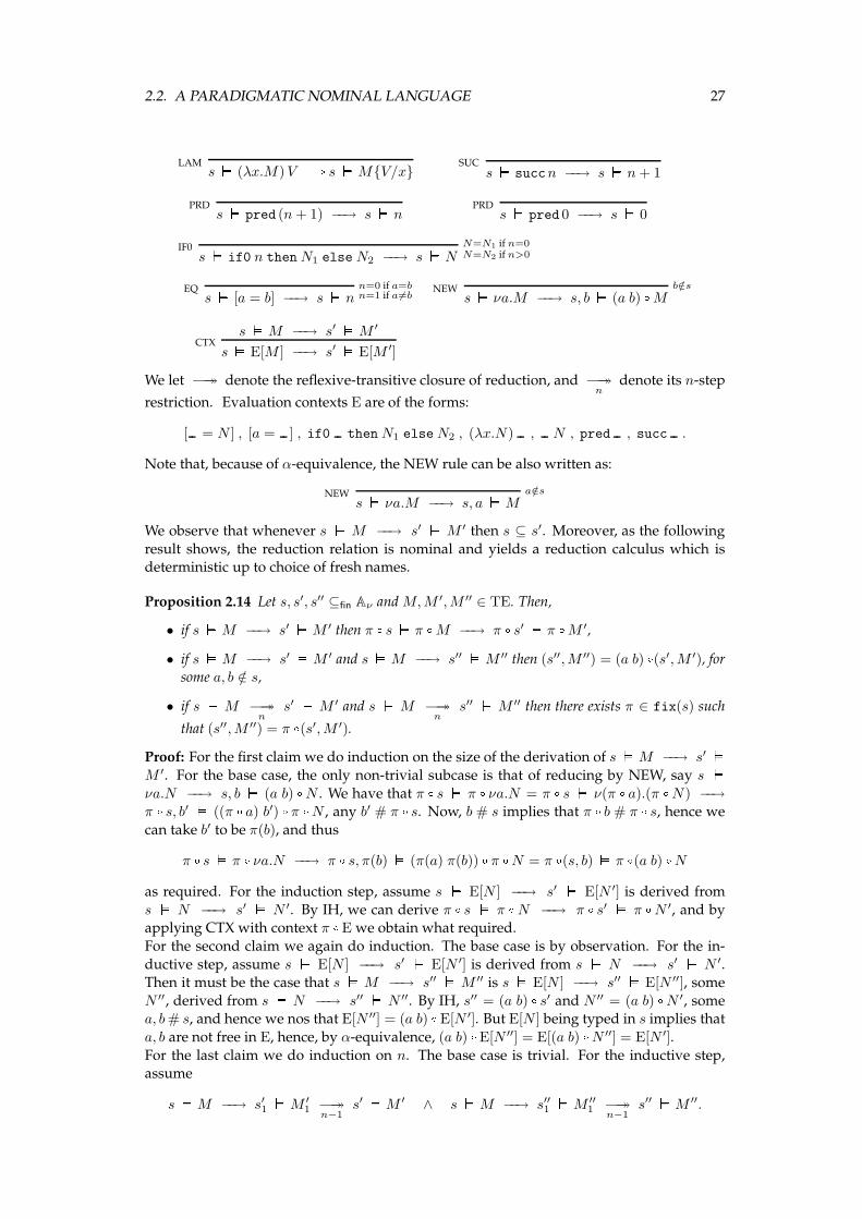
2.2. A PARADIGMATIC NOMINAL LANGUAGE 27
LAMs` (λx.M)V B s`M{V/x}
SUCs` succn −−→ s` n+ 1
PRDs` pred (n+ 1) −−→ s` n
PRDs` pred 0 −−→ s` 0
IF0 N=N1 if n=0N=N2 if n>0s` if0 n thenN1 else N2 −−→ s` N
EQ n=0 if a=bn=1 if a6=bs` [a = b] −−→ s` n
NEW b/∈s
s` νa.M −−→ s, b` (a b) [MCTX
s`M −−→ s′ `M ′
s` E[M ] −−→ s′ ` E[M ′]
We let −→→ denote the reflexive-transitive closure of reduction, and −→→n
denote its n-step
restriction. Evaluation contexts E are of the forms:
[ = N ] , [a = ] , if0 thenN1 elseN2 , (λx.N) , N , pred , succ .
Note that, because of α-equivalence, the NEW rule can be also written as:
NEW a/∈s
s` νa.M −−→ s, a`M
We observe that whenever s ` M −−→ s′ ` M ′ then s ⊆ s′. Moreover, as the following
result shows, the reduction relation is nominal and yields a reduction calculus which isdeterministic up to choice of fresh names.
Proposition 2.14 Let s, s′, s′′ ⊆fin Aν andM,M ′,M ′′ ∈ TE. Then,
• if s`M −−→ s′ `M ′ then π [ s` π [M −−→ π [ s′ ` π [M ′,
• if s`M −−→ s′ `M ′ and s`M −−→ s′′ `M ′′ then (s′′,M ′′) = (a b) [(s′,M ′), forsome a, b /∈ s,
• if s ` M −→→n
s′ ` M ′ and s ` M −→→n
s′′ ` M ′′ then there exists π ∈ fix(s) such
that (s′′,M ′′) = π [(s′,M ′).
Proof: For the first claim we do induction on the size of the derivation of s`M −−→ s′ `M ′. For the base case, the only non-trivial subcase is that of reducing by NEW, say s `νa.N −−→ s, b ` (a b) [N . We have that π [ s ` π [ νa.N = π [ s ` ν(π [a).(π [N) −−→π [ s, b′ ` ((π [a) b′) [π [N , any b′ # π [ s. Now, b # s implies that π [ b # π [ s, hence we
can take b′ to be π(b), and thus
π [ s` π [ νa.N −−→ π [ s, π(b)` (π(a) π(b)) [π [N = π [(s, b)` π [(a b) [Nas required. For the induction step, assume s ` E[N ] −−→ s′ ` E[N ′] is derived from
s ` N −−→ s′ ` N ′. By IH, we can derive π [ s ` π [N −−→ π [ s′ ` π [N ′, and byapplying CTX with context π [E we obtain what required.
For the second claim we again do induction. The base case is by observation. For the in-
ductive step, assume s ` E[N ] −−→ s′ ` E[N ′] is derived from s ` N −−→ s′ ` N ′.Then it must be the case that s ` M −−→ s′′ ` M ′′ is s ` E[N ] −−→ s′′ ` E[N ′′], some
N ′′, derived from s ` N −−→ s′′ ` N ′′. By IH, s′′ = (a b) [ s′ and N ′′ = (a b) [N ′, somea, b# s, and hence we nos that E[N ′′] = (a b) [E[N ′]. But E[N ] being typed in s implies that
a, b are not free in E, hence, by α-equivalence, (a b) [E[N ′′] = E[(a b) [N ′′] = E[N ′].
For the last claim we do induction on n. The base case is trivial. For the inductive step,assume
s`M −−→ s′1 `M ′1 −→→
n−1s′ `M ′ ∧ s`M −−→ s′′1 `M ′′
1 −→→n−1
s′′ `M ′′.
28 CHAPTER 2. NAMES, NU ANDMONADS
By our previous claims we have that (s′′1 ,m′′1) = (a b) [(s′1,m′
1) and (a b) [ s′1 ` (a b) [M ′1
−→→n−1
(a b) [ s′ ` (a b) [M ′. By IH, (s′′,M ′′) = π [(a b) [(s′,M ′), for some π ∈ fix(s′′1). But
then π ◦ (a b) ∈ fix(s), so we are done. �
Note that the notion of determinism up to fresh names is succinctly captured by support
abstraction as follows. We observe that, for every typed term s ^ Γ_M :A and any values
s′ ^ Γ_ V ′ :A and s′′ ^ Γ_ V ′′ :A,
• if s`M −→→ s′ ` V ′ and s`M −→→ s′′ ` V ′′ then [s′, V ′]s = [s′′, V ′′]s,
• if s`M −→→ s′ ` V ′ and [s′, V ′]s = [s′′, V ′′]s then s`M −→→ s′′ ` V ′′.
This allows us to define an abstract evaluation relation between terms and abstracted values,as follows.
s`M −−−→eval
[s′ ` V ′]s′′△
⇐⇒ s = s′′ ∧ s`M −→→ s′ ` V ′ (2.10)
The previous proposition implies that −−−→eval
is a well-defined partial function. More than
that, it is a total function on closed terms, as the following theorem shows.
Theorem 2.15 (SN) For any s ^∅_M :A there exist s′, V ′ such that s`M −→→ s′ ` V ′.
Proof: Shown as [Sta94, theorem 2.4]. �
2.2.2 The sν-calculus
Modelling of local state in sets of names yields a notion of unordered state, which is inade-
quate for our intended denotational semantics. Nominal game semantics is based on plays
of moves containing information about the current state. Programs are then modelled bystrategies, that is, partial functions operating on plays. These strategies, however, are de-
terministic up to choice of fresh names, a feature which is in direct conflict to unorderedstate.5
Ordered state is therefore more appropriate for our purposes. One possible approach
would be to use unordered state at the level of syntax and operational semantics of ournominal languages, and ordered state at the level of denotational semantics. In fact, this al-
ready happens with contexts: a context Γ is a set of premises, but JΓK is an (ordered) productof type-translations. Another approach would be to use ordered state both for syntactic and
semantic purposes. For the syntax this would mean to use lists of (distinct) names instead of
sets of names in local state. As lemma 2.17 suggests, one should not expect substantial dif-ferences between the two approaches. In this thesis we choose to follow the latter: ordered
state does not add much complication while it saves us from some informality.
Once we shift to ordered state, the presentation of the ν-calculus is given entirely in-side strong nominal sets. For this reason we call this version of the calculus sν-calculus,
i.e. strong ν-calculus. As mentioned above, all the nominal calculi we will examine in thesequel will de facto be “strong”.
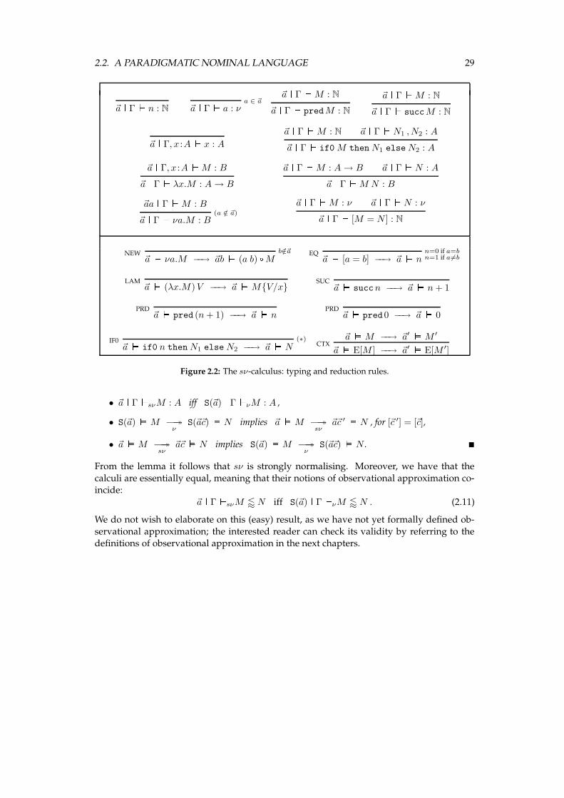
Definition 2.16 The sν-calculus shares the same syntax as the ν-calculus (page 24). Its typ-ing system is given in environments ~a^Γ and its operational semantics in environments
~a, where ~a ∈ A#ν . The rules for these are given in figure 2.2 (note we write “a ∈ ~a” for
“a ∈ S(~a)”); contexts E and the condition (∗) are as in page 27. N
The two calculi, ν and sν, are equivalent in the following sense.
Lemma 2.17 For anyM,N ∈ TE and any ~a,~a~c ∈ A#ν ,
5The problematic behaviour of nominal games in weak support is discussed again in detail in remark 3.19.
2.2. A PARADIGMATIC NOMINAL LANGUAGE 29
~a ^ Γ_ n : Na ∈ ~a
~a ^ Γ_ a : ν
~a ^ Γ_M : N
~a ^ Γ_ predM : N
~a ^ Γ_M : N
~a ^ Γ_ succM : N
~a ^ Γ, x :A_ x : A
~a ^ Γ_M : N ~a ^ Γ_N1 , N2 : A
~a ^ Γ_ if0M thenN1 elseN2 : A
~a ^ Γ, x :A_M : B
~a ^ Γ_ λx.M : A→ B
~a ^ Γ_M : A→ B ~a ^ Γ_N : A
~a ^ Γ_M N : B
~aa ^ Γ_M : B(a /∈ ~a)
~a ^ Γ_ νa.M : B
~a ^ Γ_M : ν ~a ^ Γ_N : ν
~a ^ Γ_ [M = N ] : N
NEW b/∈~a
~a` νa.M −−→ ~ab` (a b) [M EQ n=0 if a=bn=1 if a6=b~a` [a = b] −−→ ~a` n
LAM~a` (λx.M)V −−→ ~a`M{V/x}
SUC~a` succn −−→ ~a` n+ 1
PRD~a` pred (n+ 1) −−→ ~a` n
PRD~a` pred0 −−→ ~a` 0
IF0 (∗)
~a` if0 n thenN1 elseN2 −−→ ~a` N CTX~a`M −−→ ~a′ `M ′
~a` E[M ] −−→ ~a′ ` E[M ′]
Figure 2.2: The sν-calculus: typing and reduction rules.
• ~a ^ Γ_sνM : A iff S(~a) ^ Γ_νM : A ,
• S(~a)`M −→→ν
S(~a~c) ` N implies ~a`M −→→sν
~a~c ′ ` N , for [~c ′] = [~c],
• ~a`M −→→sν
~a~c` N implies S(~a)`M −→→ν
S(~a~c) ` N . �
From the lemma it follows that sν is strongly normalising. Moreover, we have that the
calculi are essentially equal, meaning that their notions of observational approximation co-incide:
~a ^ Γ_sνM / N iff S(~a) ^ Γ_νM / N . (2.11)
We do not wish to elaborate on this (easy) result, as we have not yet formally defined ob-
servational approximation; the interested reader can check its validity by referring to thedefinitions of observational approximation in the next chapters.
30 CHAPTER 2. NAMES, NU ANDMONADS
2.3 Monads and Comonads
In this section we present some basic results on the categorical constructions we will beusing in the following chapters. Some basic category theory is assumed, covering notions
such as products, coproducts, adjoints, etc. (see e.g. [Mac98]).Monads and comonads are standard categorical notions (v. [Mac98] and [BW99, “triples”])
which have been used extensively in denotational semantics of programming languages in
order to encapsulate computation. The success of these constructions is due to their con-ceptual simplicity: definitions involve nothing more than ome natural transformations and
commuting diagrams. Combining monads is not always an easy (or even possible) task,and this is their main defect. However, the monads we use in this thesis combine relatively
well.
2.3.1 Monads
Monads were introduced in denotational semantics through the work of Moggi [Mog89,Mog91], who proposed them as a generic tool for encapsulating computational effects.
Wadler [Wad92, Wad95] popularised monads in programming as a means of simulatingeffects in functional programs, and nowadays monads form part and parcel of the Haskell
programming language [Jon03].
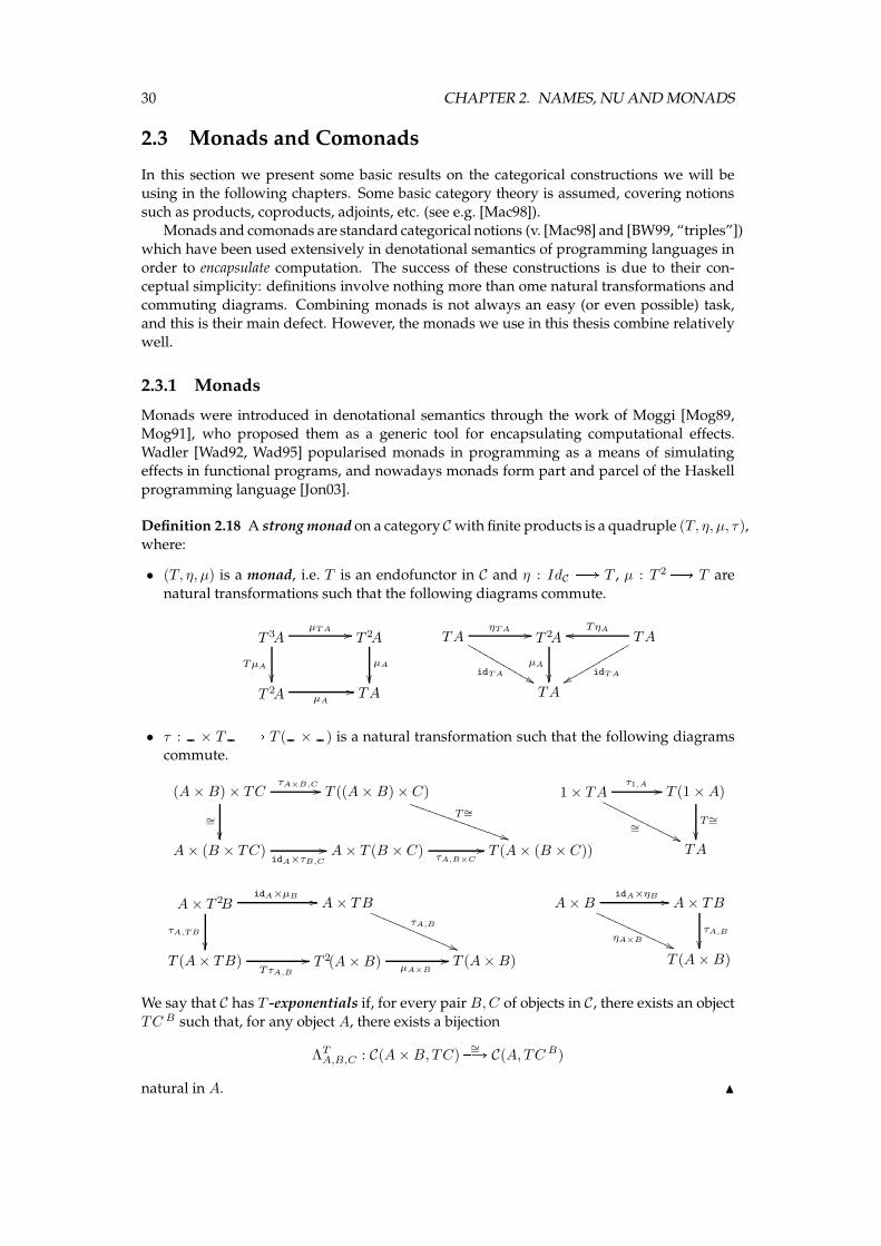
Definition 2.18 A strongmonad on a category C with finite products is a quadruple (T, η, µ, τ),
where:
• (T, η, µ) is a monad, i.e. T is an endofunctor in C and η : IdC B T , µ : T 2 B T are
natural transformations such that the following diagrams commute.
T 3AµT A //
TµA
��
T 2A
µA
��T 2A µA
// TA
TAηT A //
idT A &&MMMMMMMMMMM T 2A
µA
��
TATηAoo
idT Axxrrrrrrrrrrr
TA
• τ : × T B T ( × ) is a natural transformation such that the following diagramscommute.
(A×B) × TCτA×B,C //
∼=
��
T ((A× B) × C)
T∼=
))SSSSSSSSSSSSSSS
A× (B × TC)idA×τB,C
// A× T (B × C) τA,B×C
// T (A× (B × C))
1 × TAτ1,A //
∼=''OOOOOOOOOOOO
T (1 ×A)
T∼=
��TA
A× T 2BidA×µB //
τA,TB
��
A× TBτA,B
((QQQQQQQQQQQQQ
T (A× TB)TτA,B
// T 2(A×B) µA×B
// T (A×B)
A×BidA×ηB //
ηA×B ((PPPPPPPPPPPPA× TB
τA,B
��T (A×B)
We say that C has T -exponentials if, for every pair B,C of objects in C, there exists an object
TC B such that, for any object A, there exists a bijection
ΛTA,B,C : C(A×B, TC)∼=PA C(A, TC B)
natural in A. N
2.3. MONADS AND COMONADS 31
Given a strong monad (T, η, µ, τ), we define τ ′ : T ( ) × B T ( × ) as follows.
τ ′A,B : TA×B∼=PA B × TA
τB,APPPPA T (B ×A)∼=PA T (A×B) (2.12)
τ ′ satisfies the corresponding strength equations. Wemay refer to τ as right strength and to τ ′
as left strength. Combining strengths and multiplications we obtain natural transformations:
ψA,B : TA× TBτ ′
A,T BPPPPPA T (A× TB)TτA,BPPPPPA T 2(A×B)
µA×BPPPPA T (A×B) ,
ψ′A,B : TA× TB
τTA,BPPPPPA T (TA×B)Tτ ′
A,BPPPPPA T 2(A×B)µA×BPPPPA T (A×B) .
(2.13)
T -exponentials supply us with of T -evaluation arrows, that is,
evTB,C : TC B ×BB TC , ΛT−1
(idTCB ) (2.14)
so that, for each f : A×BB TC, the following diagram commutes.
(TC)B ×Bev
T
// TC
A×B
ΛT (f)×id
OO
f
99tttttttttttt
T -exponentiation is in fact a functor (T )− : C op × C B C which takes each f : A′ B A
and g : B′ B B to
Tg f : TB′A B TBA′
, ΛT (TB′A ×A′ id × fPPPPPA TB′A ×Aev
TPPPA TB′ TgPPA TB) . (2.15)
Finally, monads on a given category form a category of their own by use of the following
notion.
Definition 2.19 Let (T, η, µ, τ) and (T , η, µ, τ ) be strong monads on a category C. A monad
morphism a : (T, η, µ, τ) B (T , η, µ, τ ) is a natural transformation a : T B T making thefollowing diagrams commute.
AηA //
ηA
!!DDD
DDDD
DDDD
TA
aA
��TA
T 2A
aT A ; T aA
��
µA // TA
aA
��T 2A µA
// TA
A× TBτA,B //
idA×aB
��
T (A×B)
aA×B
��A× TB τA,B
// T (A×B)N
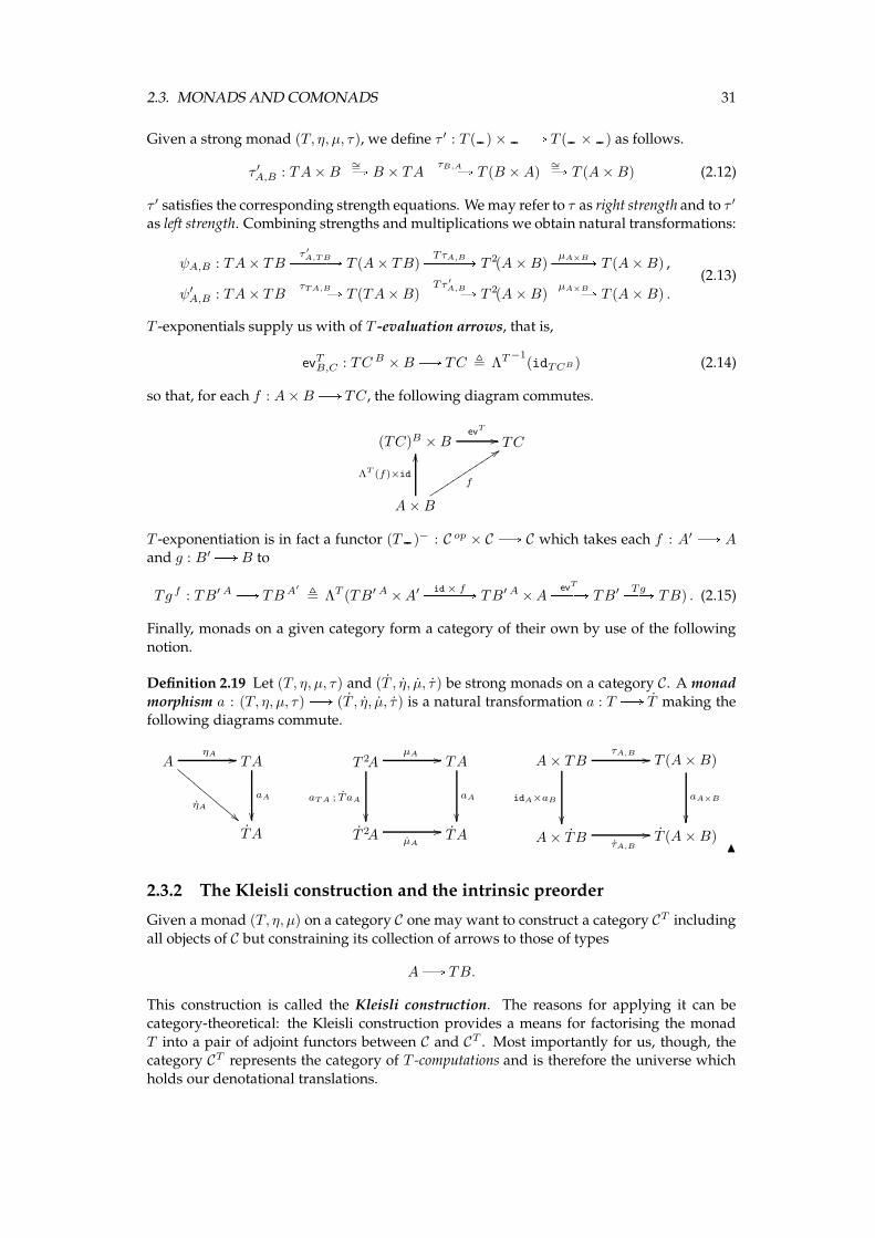
2.3.2 The Kleisli construction and the intrinsic preorder
Given a monad (T, η, µ) on a category C one may want to construct a category CT including
all objects of C but constraining its collection of arrows to those of types
AB TB.
This construction is called the Kleisli construction. The reasons for applying it can be
category-theoretical: the Kleisli construction provides a means for factorising the monad
T into a pair of adjoint functors between C and CT . Most importantly for us, though, thecategory CT represents the category of T -computations and is therefore the universe which
holds our denotational translations.
32 CHAPTER 2. NAMES, NU ANDMONADS
Definition 2.20 Let C be a category and (T, η, µ) be a monad on C. The Kleisli category CT
contains the same objects as C and, for all objects A,B,
CT (A,B) , C(A, TB) .
Moreover, the identity arrow on A is ηA , and composition of arrows f : A B TB andg : BB TC is given by:
AfPA TB
TgPPA T 2CµPA TC .
N
If C has finite products then T being a strong monad corresponds to CT having a symmetricpremonoidal tensor, that is, a non-bifunctorial tensor product (see [PR97]), which allows us
to model computation products in CT . Furthermore, the requirement for T -exponentialsmakes the premonoidal structure of CT closed (and corresponds to closure of the related
Freyd category, see [Pow00]).
Intrinsic preorder The notion of equating programs modulo their observable behaviourcan be modelled categorically by means of quotienting by the intrinsic preorder. So let us
assume that T is a strong monad with exponentials on C and that there is a distinguishedobject o of C corresponding to a type of observables. We fix a collection
O ⊆ C(1, T o)
of arrows of specific observable behaviour and build the intrinsic preorder on arrows asfollows.6
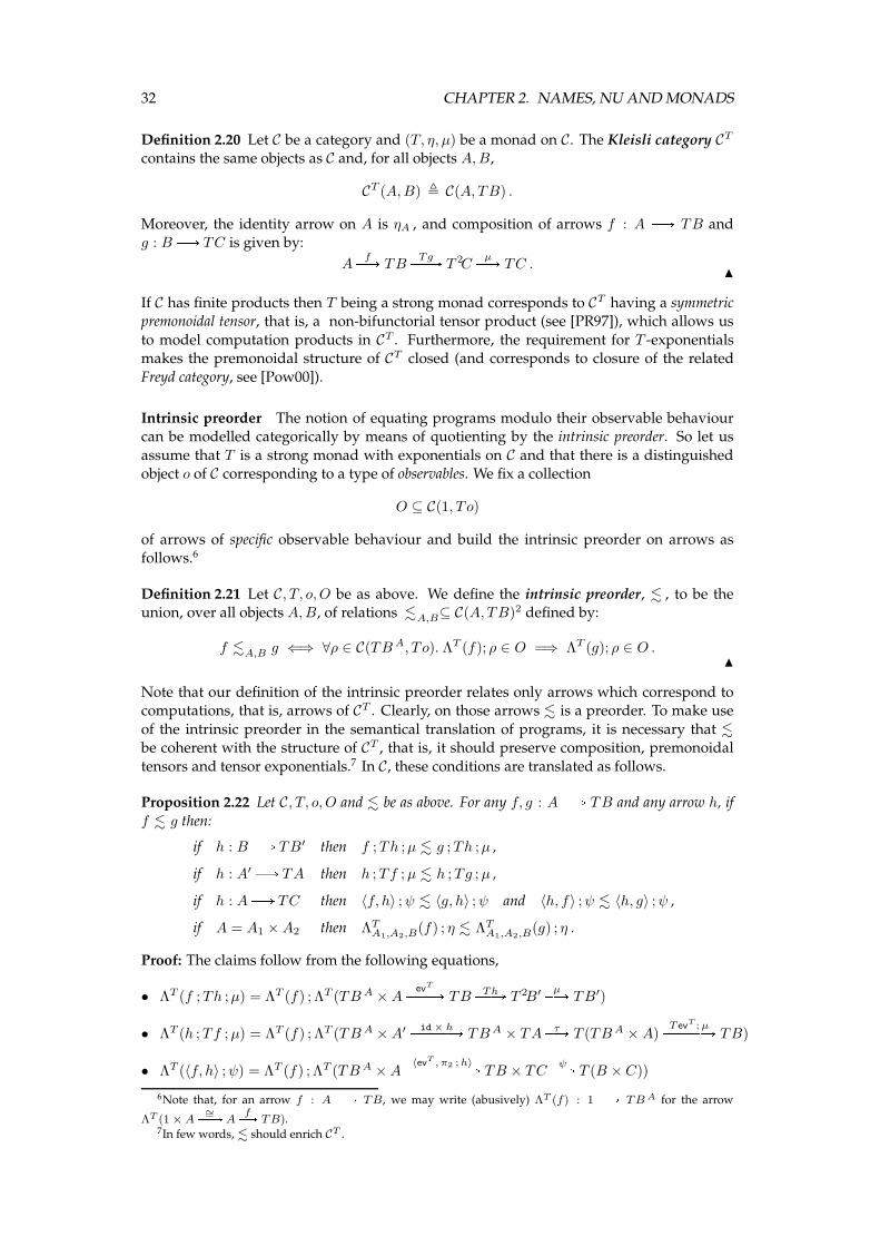
Definition 2.21 Let C, T, o, O be as above. We define the intrinsic preorder, . , to be theunion, over all objects A,B, of relations .A,B⊆ C(A, TB)2 defined by:
f .A,B g ⇐⇒ ∀ρ ∈ C(TBA, T o). ΛT (f); ρ ∈ O =⇒ ΛT (g); ρ ∈ O .N
Note that our definition of the intrinsic preorder relates only arrows which correspond tocomputations, that is, arrows of CT . Clearly, on those arrows . is a preorder. To make use
of the intrinsic preorder in the semantical translation of programs, it is necessary that .be coherent with the structure of CT , that is, it should preserve composition, premonoidal
tensors and tensor exponentials.7 In C, these conditions are translated as follows.
Proposition 2.22 Let C, T, o, O and . be as above. For any f, g : AB TB and any arrow h, if
f . g then:
if h : BB TB′ then f ;Th ;µ . g ;Th ;µ ,
if h : A′ B TA then h ;Tf ;µ . h ;Tg ;µ ,
if h : AB TC then 〈f, h〉 ;ψ . 〈g, h〉 ;ψ and 〈h, f〉 ;ψ . 〈h, g〉 ;ψ ,
if A = A1 ×A2 then ΛTA1,A2,B(f) ; η . ΛTA1,A2,B
(g) ; η .
Proof: The claims follow from the following equations,
• ΛT (f ;Th ;µ) = ΛT (f) ; ΛT (TB A ×Aev
TPPPA TB ThPPA T 2B′ µPA TB′)
• ΛT (h ;Tf ;µ) = ΛT (f) ; ΛT (TB A ×A′ id × hPPPPPA TBA × TA τPA T (TBA ×A)T ev
T ; µPPPPPA TB)
• ΛT (〈f, h〉 ;ψ) = ΛT (f) ; ΛT (TB A ×A〈evT , π2 ;h〉PPPPPPPPA TB × TC
ψPA T (B × C))
6Note that, for an arrow f : A B TB, we may write (abusively) ΛT (f) : 1 B TBA for the arrow
ΛT (1 × A∼=PPA A
fPA TB).7In few words, . should enrich CT .
2.3. MONADS AND COMONADS 33
• ΛT (ΛT (f) ; η) = ΛT (f) ; ΛT (TB A1×A2 ×A1ΛT (evT )PPPPPPA TB A2
ηPA T (TBA2))
which are true due to naturality of ΛT . �
Let us remark here that we will not be making actual use of the Kleisli construction in thesemantical models of the following chapters. Rather, we will remain at the base semantical
categories andmake use of properties coming from the categories’ Kleisli counterparts, suchas the intrinsic preorder properties of the previous proposition.
2.3.3 Defining side-effects
Given a strong monad with exponentials and any object ξ of C, we can form a ξ-side-effect
monad on C as follows (cf. [Mog88]).
Proposition and Definition 2.23 Let (T, η, µ, τ) be a strong monad with exponentials on C andlet ξ be an object of C. Form the quadruple (T , η, µ, τ ) by taking:
• T : C B C , T ( × ξ) ξ ,
• ηA : AB TA , ΛT (ηA) ,
• µA : T 2AB TA , ΛT (µA) ,
• τA,B : A× TBB T (A×B) , ΛT (τA,B) ;
• ηA , A× ξηPA T (A× ξ) ,
• µA , T 2A× ξev
TPPA T (TA× ξ)T ev
TPPPPA T 2(A× ξ)µPA T (A× ξ) ,
• τA,B , A× TB × ξid × ev
TPPPPPPA A× T (B × ξ) τPA T (A×B × ξ) .
Then (T , η, µ, τ) is a strong monad on C. Moreover, we obtain T -exponentials by taking, for each
A,B,C and any f : A×BB TC, g : AB TC B ,
TAB , TAB×ξ
ΛT (f) , ΛTA,B×ξ,C×ξ(ΛTA×B,ξ,C×ξ
−1(f))
ΛT−1
(g) , ΛTA×B,ξ,C×ξ(ΛTA,B×ξ,C×ξ
−1(g)) .
Proof: Standard result [Mog88]. �
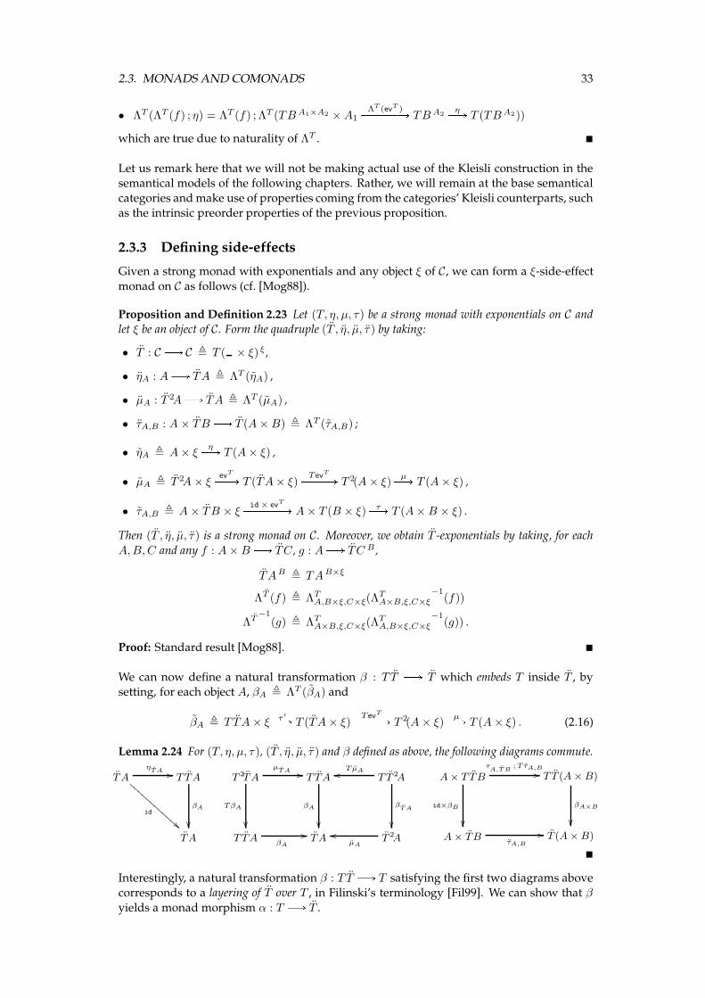
We can now define a natural transformation β : T T B T which embeds T inside T , bysetting, for each object A, βA , ΛT (βA) and
βA , T TA× ξ τ ′PA T (TA× ξ)T ev
TPPPPA T 2(A× ξ)µPA T (A× ξ) . (2.16)
Lemma 2.24 For (T, η, µ, τ), (T , η, µ, τ ) and β defined as above, the following diagrams commute.
TAη
T A //
id
!!BBB
BBBB
BBBB
B T TA
βA
��TA
T 2TAµ
T A //
TβA
��
T TA
βA
��
T T 2ATµAoo
βT A
��T TA
βA
//TA T 2A
µA
oo
A × T TBτ
A,T B;TτA,B//
id×βB
��
T T (A × B)
βA×B
��A × TB
τA,B
// T (A × B)
�
Interestingly, a natural transformation β : T T B T satisfying the first two diagrams abovecorresponds to a layering of T over T , in Filinski’s terminology [Fil99]. We can show that β
yields a monad morphism α : T B T .
34 CHAPTER 2. NAMES, NU ANDMONADS
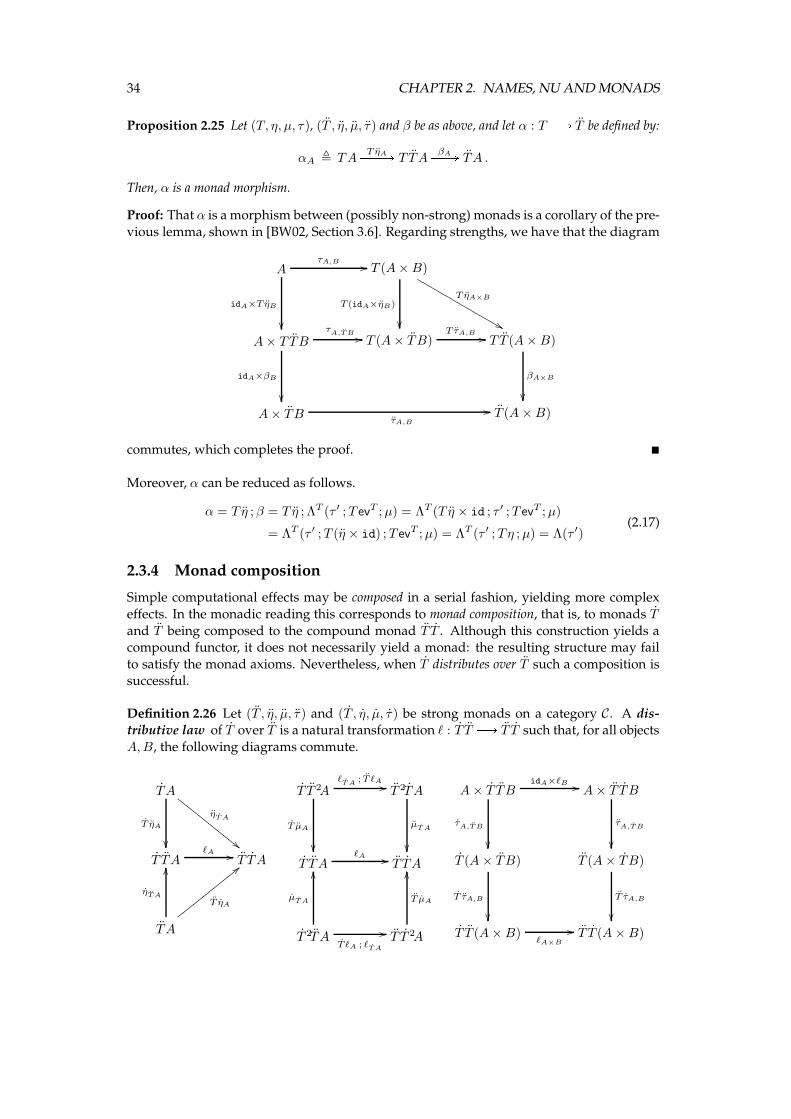
Proposition 2.25 Let (T, η, µ, τ), (T , η, µ, τ) and β be as above, and let α : T B T be defined by:
αA , TAT ηAPPPA T TA
βAPPA TA .
Then, α is a monad morphism.
Proof: That α is a morphism between (possibly non-strong) monads is a corollary of the pre-
vious lemma, shown in [BW02, Section 3.6]. Regarding strengths, we have that the diagram
AτA,B //
idA×T ηB
��
T (A×B)
T (idA×ηB)
��
T ηA×B
&&LLLLLLLLLLLLLLL
A× T TBτA,T B //
idA×βB
��
T (A× TB)T τA,B // T T (A×B)
βA×B
��A× TB
τA,B
// T (A×B)
commutes, which completes the proof. �
Moreover, α can be reduced as follows.
α = T η ;β = T η ; ΛT (τ ′ ;T evT ;µ) = ΛT (T η × id ; τ ′ ;T evT ;µ)
= ΛT (τ ′ ;T (η × id) ;T evT ;µ) = ΛT (τ ′ ;Tη ;µ) = Λ(τ ′)(2.17)
2.3.4 Monad composition
Simple computational effects may be composed in a serial fashion, yielding more complex
effects. In the monadic reading this corresponds to monad composition, that is, to monads T
and T being composed to the compound monad T T . Although this construction yields acompound functor, it does not necessarily yield a monad: the resulting structure may fail
to satisfy the monad axioms. Nevertheless, when T distributes over T such a composition issuccessful.
Definition 2.26 Let (T , η, µ, τ ) and (T , η, µ, τ ) be strong monads on a category C. A dis-
tributive law of T over T is a natural transformation ℓ : T T B T T such that, for all objects
A,B, the following diagrams commute.
TA
T ηA
��
ηT A
""EEEEEEE
EEEEE
T TAℓA // T TA
TA
ηT A
OO
T ηA
<<yyyyyyyyyyyy
T T 2A
T µA
��
ℓT A ; T ℓA // T 2TA
µT A
��T TA
ℓA // T TA
T 2TAT ℓA ; ℓTA
//
µT A
OO
T T 2A
T µA
OO
A× T TBidA×ℓB //
τA,TB
��
A× T TB
τA,TB
��T (A× TB)
T τA,B
��
T (A× TB)
T τA,B
��T T (A×B)
ℓA×B
// T T (A×B)
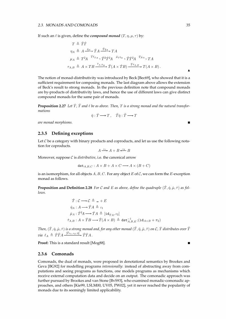
2.3. MONADS AND COMONADS 35
If such an ℓ is given, define the compound monad (T, η, µ, τ) by:
T , T T
ηA , AηAPPA TA
T ηAPPPA TA
µA , T 2AT ℓTAPPPPA T 2T 2A
µT2APPPPA T T 2AT µAPPPA TA
τA,B , A× TBτA,TBPPPPA T (A× TB)
T τA,BPPPPPA T (A×B) .N
The notion of monad-distributivity was introduced by Beck [Bec69], who showed that it is a
sufficient requirement for composing monads. The last diagram above allows the extensionof Beck’s result to strong monads. In the previous definition note that compound monads
are by-products of distributivity laws, and hence the use of different laws can give distinct
compound monads for the same pair of monads.
Proposition 2.27 Let T , T and ℓ be as above. Then, T is a strong monad and the natural transfor-
mationsη : T B T , T η : T B T
are monad morphisms. �
2.3.5 Defining exceptions
Let C be a category with binary products and coproducts, and let us use the following nota-
tion for coproducts.A
ι1PA A+Bι2QP B
Moreover, suppose C is distributive, i.e. the canonical arrow
dstA,B,C : A× B +A× CB A× (B + C)
is an isomorphism, for all objectsA,B,C. For any objectE of C, we can form theE-exception
monad as follows.
Proposition and Definition 2.28 For C and E as above, define the quadruple (T , η, µ, τ ) as fol-
lows.
T : C B C , + E
ηA : AB TA , ι1
µA : T 2AB TA , [idTA, ι2]
τA,B : A× TBB T (A×B) , dst−1A,B,E ;(idA×B + π2)
Then, (T , η, µ, τ ) is a strong monad and, for any other monad (T , η, µ, τ) on C, T distributes over T
via ℓA , T TA[T ι1, ι2; η]PPPPPPPA T TA .
Proof: This is a standard result [Mog88]. �
2.3.6 Comonads
Comonads, the dual of monads, were proposed in denotational semantics by Brookes and
Geva [BG92] for modelling programs intensionally: instead of abstracting away from com-putations and seeing programs as functions, one models programs as mechanisms which
receive external computation data and decide on an output. The comonadic approach was
further pursued by Brookes and van Stone [BvS93], who examined monadic-comonadic ap-proaches, and others [Kie99, LSLM00, UV05, PW02], yet it never reached the popularity of
monads due to its seemingly limited applicability.

36 CHAPTER 2. NAMES, NU ANDMONADS
Definition 2.29 A comonad on a category C is a triple (Q, ε, δ), where Q is an endofunctorin C and ε : Q B IdC , δ : Q B Q2 are natural transformations such that the following
diagrams commute.
QA
δA
��
δA // Q2A
QδA
��Q2A
δQA
// Q3A
QA
δA
��
idQA
yyrrrrrrrrrrridQA
%%LLLLLLLLLLL
QA Q2AεQA
ooQεA
// QAN
In case C has products, we define a transformation ζ : Q( × )B ×Q( ),
ζA,B : Q(A×B)〈Qπ1, Qπ2〉PPPPPPPPA QA×QB
εA × idQBPPPPPPPPA A×QB (2.18)
which makes the (comonadic) strength-diagrams commute.
Lemma 2.30 Let (Q, ε, δ) be a comonad on a category C with finite products. Then, ζ makes thefollowing diagrams commute.
(A×B) ×QC Q((A×B) × C)z A×B,Coo
A× (B ×QC)
∼=
OO
A×Q(B × C)idA× z B,C
oo Q(A× (B × C))z A,B×C
oo
Q∼=iiTTTTTTTTTTTTTTT
1 ×QA Q(1 ×A)z 1,Aoo
QA
∼=
ggOOOOOOOOOOOOO
Q∼=
OO
A×Q2B A×QBidA×δBoo
Q(A×QB)
z A,QB
OO
Q2(A×B)Q z A,B
oo Q(A×B)δA×B
oo
z A,B
hhPPPPPPPPPPPPP
A×B A×QBidA×εBoo
Q(A×B)
z A,B
OO
εA×B
ggOOOOOOOOOOO
Proof: This follows easily from the comonadic properties; we show the last two cases.
ζA,B ; idA × εB = 〈Qπ1, Qπ2〉 ; εA × idQB ; idA × εB = 〈Qπ1 ; εA, Qπ2 ; εB〉
= 〈εA×B ;π1, εA×B ;π2〉 = εA×B
δA×B ;Q ζA,B ; ζA,QB = δA×B ;Q〈Qπ1, Qπ2〉 ;Q(εA × idQB) ;〈Qπ1, Qπ2〉 ; εA × idQ2B
= δA×B ;Q〈Qπ1, Qπ2〉 ;〈Qπ1 ;QεA, Qπ2〉 ; εA × idQ2B
= δA×B ;Q〈Qπ1, Qπ2〉 ;〈Qπ1, Qπ2〉 ;(QεA ; εA) × idQ2B
= δA×B ;〈Q2π1, Q2π2〉 ;(QεA ; εA) × idQ2B
= 〈Qπ1 ; δA, Qπ2 ; δB〉 ;(QεA ; εA) × idQ2B
= 〈Qπ1 ; εA, Qπ2 ; δB〉 = ζA×B ; idA × δB�
Stronger comonads are obtained by stipulating a transformation ζ in the other direction, asin the case of strong comonads of [BvS93]. In our case, we stipulate even stronger conditions.
Definition 2.31 A comonad (Q, ε, δ) with transformation ζ defined as above is called aproduct comonad if ζ is a natural isomorphism. N
We write ζ : × Q( ) B Q( × ) for the inverse of ζ . Moreover, and as in the caseof monadic strengths, we let ζ ′, ζ ′ be their symmetric counterparts. Note that a product
comonad Q can be written asQ ∼= Q1 × (2.19)
hence the name.8 We say that Q1 is the basis of the comonad.
8Note this is an isomorphism between comonads, not merely between functors.
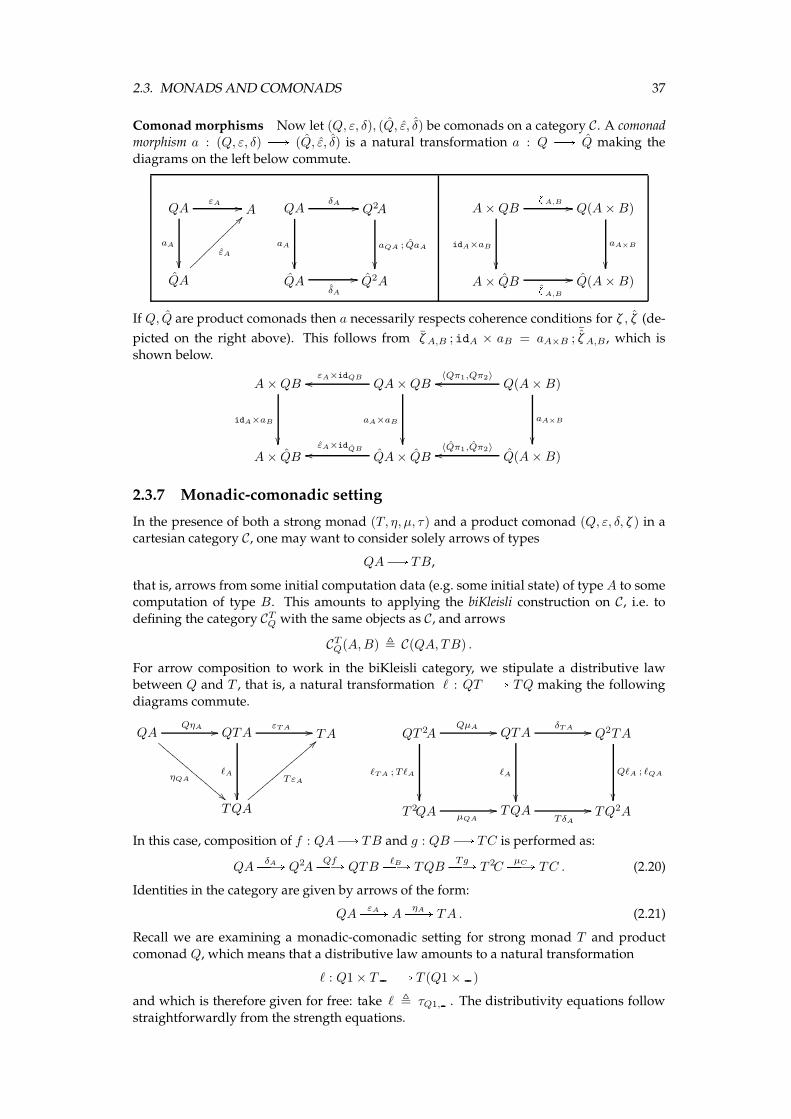
2.3. MONADS AND COMONADS 37
Comonad morphisms Now let (Q, ε, δ), (Q, ε, δ) be comonads on a category C. A comonadmorphism a : (Q, ε, δ) B (Q, ε, δ) is a natural transformation a : Q B Q making the
diagrams on the left below commute.
QAεA //
aA
��
A
QA
εA
??~~~~~~~~~~~
QAδA //
aA
��
Q2A
aQA ; QaA
��QA
δA
// Q2A
A×QBzA,B //
idA×aB
��
Q(A×B)
aA×B
��A× QB zA,B
// Q(A×B)
If Q, Q are product comonads then a necessarily respects coherence conditions for ζ , ζ (de-
picted on the right above). This follows from ζA,B ; idA × aB = aA×B ;¯ζA,B , which is
shown below.
A×QB
idA×aB
��
QA×QB
aA×aB
��
εA×idQBoo Q(A×B)〈Qπ1,Qπ2〉oo
aA×B
��A× QB QA× QB
εA×idQBoo Q(A×B)〈Qπ1,Qπ2〉oo
2.3.7 Monadic-comonadic setting
In the presence of both a strong monad (T, η, µ, τ) and a product comonad (Q, ε, δ, ζ ) in acartesian category C, one may want to consider solely arrows of types
QAB TB,
that is, arrows from some initial computation data (e.g. some initial state) of type A to somecomputation of type B. This amounts to applying the biKleisli construction on C, i.e. todefining the category CTQ with the same objects as C, and arrows
CTQ(A,B) , C(QA, TB) .
For arrow composition to work in the biKleisli category, we stipulate a distributive lawbetween Q and T , that is, a natural transformation ℓ : QT B TQ making the following
diagrams commute.
QAQηA //
ηQA
!!DDD
DDDD
DDDD
DDD
QTA
ℓA
��
εT A // TA
TQA
TεA
==zzzzzzzzzzzzzz
QT 2AQµA //
ℓTA ;TℓA
��
QTA
ℓA
��
δT A // Q2TA
QℓA ; ℓQA
��T 2QA µQA
// TQATδA
// TQ2A
In this case, composition of f : QAB TB and g : QBB TC is performed as:
QAδAPPA Q2A
QfPPA QTBℓBPPA TQB
TgPPA T 2CµCPPA TC . (2.20)
Identities in the category are given by arrows of the form:
QAεAPPA A
ηAPPA TA . (2.21)
Recall we are examining a monadic-comonadic setting for strong monad T and product
comonad Q, which means that a distributive law amounts to a natural transformation
ℓ : Q1 × T B T (Q1 × )
and which is therefore given for free: take ℓ , τQ1, . The distributivity equations follow
straightforwardly from the strength equations.
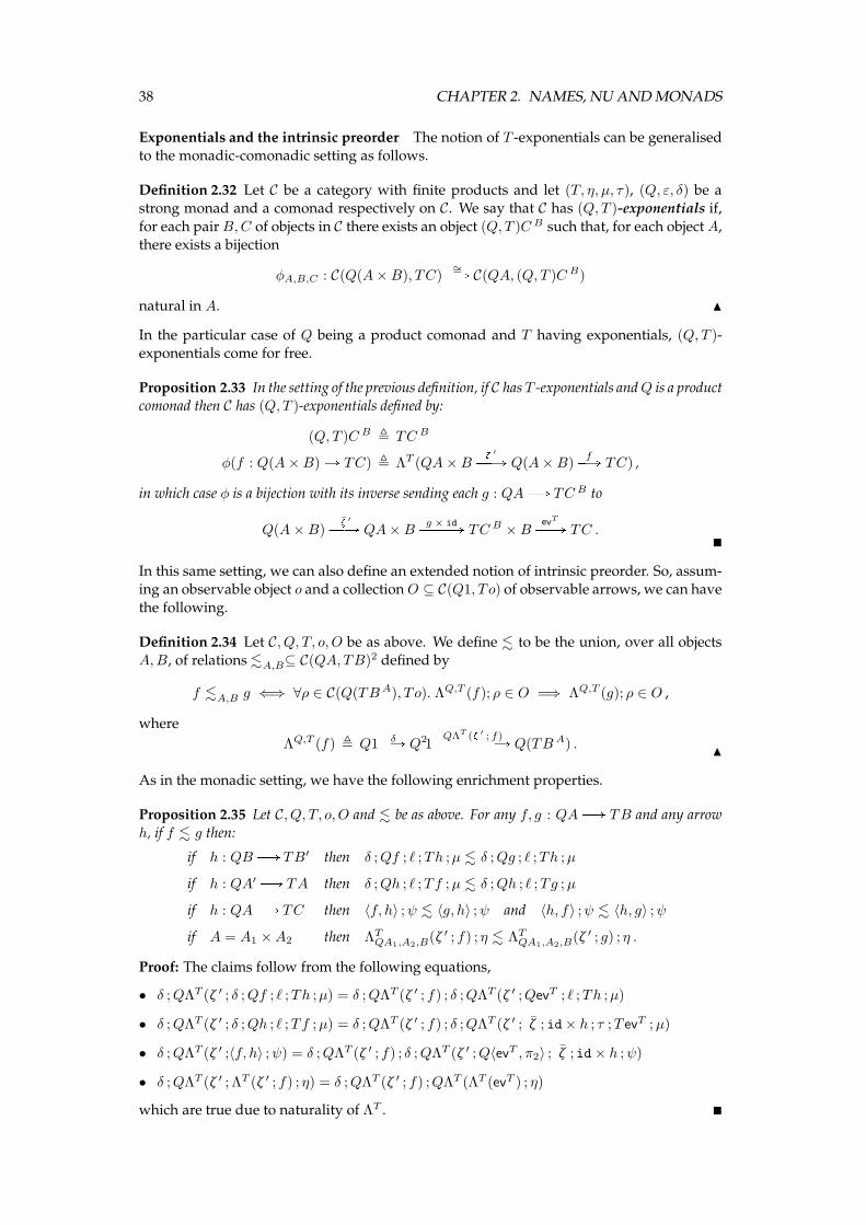
38 CHAPTER 2. NAMES, NU ANDMONADS
Exponentials and the intrinsic preorder The notion of T -exponentials can be generalisedto the monadic-comonadic setting as follows.
Definition 2.32 Let C be a category with finite products and let (T, η, µ, τ), (Q, ε, δ) be astrong monad and a comonad respectively on C. We say that C has (Q, T )-exponentials if,
for each pairB,C of objects in C there exists an object (Q, T )C B such that, for each object A,there exists a bijection
φA,B,C : C(Q(A×B), TC)∼=PA C(QA, (Q, T )C B)
natural in A. N
In the particular case of Q being a product comonad and T having exponentials, (Q, T )-exponentials come for free.
Proposition 2.33 In the setting of the previous definition, if C has T -exponentials andQ is a productcomonad then C has (Q, T )-exponentials defined by:
(Q, T )C B , TC B
φ(f : Q(A×B)A TC) , ΛT (QA×Bz ′PPA Q(A×B)
fPA TC) ,
in which case φ is a bijection with its inverse sending each g : QAB TC B to
Q(A×B)z ′PPA QA×B
g × idPPPPA TC B ×Bev
TPPA TC .�
In this same setting, we can also define an extended notion of intrinsic preorder. So, assum-ing an observable object o and a collectionO ⊆ C(Q1, T o) of observable arrows, we can have
the following.
Definition 2.34 Let C, Q, T, o,O be as above. We define . to be the union, over all objectsA,B, of relations .A,B⊆ C(QA, TB)2 defined by
f .A,B g ⇐⇒ ∀ρ ∈ C(Q(TBA), T o). ΛQ,T (f); ρ ∈ O =⇒ ΛQ,T (g); ρ ∈ O ,
where
ΛQ,T (f) , Q1 δPA Q21QΛT (z ′ ; f)PPPPPPPPA Q(TB A) . N
As in the monadic setting, we have the following enrichment properties.
Proposition 2.35 Let C, Q, T, o,O and . be as above. For any f, g : QAB TB and any arrowh, if f . g then:
if h : QBB TB′ then δ ;Qf ; ℓ ;Th ;µ . δ ;Qg ; ℓ ;Th ;µ
if h : QA′ B TA then δ ;Qh ; ℓ ;Tf ;µ . δ ;Qh ; ℓ ;Tg ;µ
if h : QAB TC then 〈f, h〉 ;ψ . 〈g, h〉 ;ψ and 〈h, f〉 ;ψ . 〈h, g〉 ;ψ
if A = A1 ×A2 then ΛTQA1,A2,B(ζ ′ ; f) ; η . ΛTQA1,A2,B
(ζ ′ ; g) ; η .
Proof: The claims follow from the following equations,
• δ ;QΛT (ζ ′ ; δ ;Qf ; ℓ ;Th ;µ) = δ ;QΛT (ζ ′ ; f) ; δ ;QΛT (ζ ′ ;QevT ; ℓ ;Th ;µ)
• δ ;QΛT (ζ ′ ; δ ;Qh ; ℓ ;Tf ;µ) = δ ;QΛT (ζ ′ ; f) ; δ ;QΛT (ζ ′ ; ζ ; id× h ; τ ;T evT ;µ)
• δ ;QΛT (ζ ′ ;〈f, h〉 ;ψ) = δ ;QΛT (ζ ′ ; f) ; δ ;QΛT (ζ ′ ;Q〈evT , π2〉 ; ζ ;id× h ;ψ)
• δ ;QΛT (ζ ′ ; ΛT (ζ ′ ; f) ; η) = δ ;QΛT (ζ ′ ; f) ;QΛT (ΛT (evT ) ; η)
which are true due to naturality of ΛT . �
Chapter 3
Nominal Games
Nominal games were introduced in [AGM+04, Lai04] as a basis for the fully abstract mod-elling of nominal computation. They constitute a reformulation of ordinary games in nomi-
nal sets,1 thus allowing for names (atoms) to appear in plays as atomic moves and therefore
for strategies to involve (equivariant) name-reasoning.In this thesis we follow the presentation of [AGM+04] (the AGMOS approach), rectifying
also discrepancies arising in [AGM+04] from the incompatibility of unordered state withdeterminacy of strategies. Two further guidelines for (our) nominal games are the following.
• Use of moves with local state attached, a notion that had been used before by Ong for
the semantics of Idealized Algol [Ong02].
• Use of call-by-value discipline, as advanced by Honda and Yoshida [HY99] for thesemantics of call-by-value PCF.
These stem from the fact that the languageswe examine are stateful subsets ofML [MTM97].
With regard to local state, our approach coincides with the AGMOS approach in that movesinside a play are attached with the full list of names available at the computation step they
represent. This is advantageous in that it is simple and allows for better control over plays
and strategies, witnessed e.g. by the concise proof of adequacy in the next chapter. More-over, the approach is easily customisable to nominal languages with a variety of effects:
once the denotational framework for names has been set, further nominal effects can bemodelled by use of monads. Here this is exemplified through general references (chapter 4)
and exceptions (chapter 5).
On the other hand, full access to local names and the use of monads for effects allowstrategies to make too many distinctions at the intentional level and therefore our full-
abstraction results rely on quotienting. Stricter approaches to local state followed in [Lai08,
MT09], for languages with ground store, factor out such distinctions and lead to fully ab-stract models without quotienting. Those models make use of a local state that includes only
those names that have been used and are still available, for appropriate notions of name-useand name-availability. Naturally, the added strictness comes with a cost of added com-
plicacy in the manipulation of strategies and, in fact, the methods are no longer generic:
different languages have different notions of name-use, name-availability and local state. Inparticular, the approach is not applicable to general references— at least not directly. See
section 3.5 for further discussion.The chapter is structured as follows. In section 3.1we introduce the basic notions of nom-
inal games, that is, nominal arenas, plays and strategies. We work on play- and strategy-
composition and obtain the category G of nominal arenas and nominal strategies. In sec-tion 3.2 we focus on innocence, and produce the subcategory V of innocent strategies. In
section 3.3 we further restrict ourselves to total strategies and obtain the category Vt, which
1Although nominal sets are not explicitly mentioned in [Lai04], they are in the journal version of the pa-per [Lai08].
39
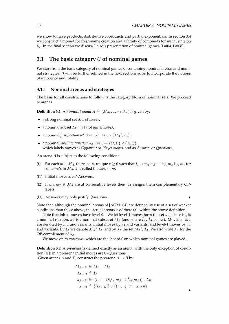
40 CHAPTER 3. NOMINAL GAMES
we show to have products, distributive coproducts and partial exponentials. In section 3.4we construct a monad for fresh-name creation and a family of comonads for initial state on
Vt. In the final section we discuss Laird’s presentation of nominal games [Lai04, Lai08].
3.1 The basic category G of nominal games
We start from the basic category of nominal games G, containing nominal arenas and nomi-
nal strategies. G will be further refined in the next sections so as to incorporate the notionsof innocence and totality.
3.1.1 Nominal arenas and strategies
The basis for all constructions to follow is the category Nom of nominal sets. We proceed
to arenas.
Definition 3.1 A nominal arena A , (MA, IA,⊢A, λA) is given by:
• a strong nominal setMA of moves,
• a nominal subset IA ⊆MA of initial moves,
• a nominal justification relation ⊢A⊆MA × (MA \ IA),
• a nominal labelling function λA : MA → {O,P} × {A,Q},which labels moves as Opponent or Player moves, and as Answers or Questions.
An arena A is subject to the following conditions.
(f) For eachm ∈MA, there exists unique k ≥ 0 such that IA ∋ m1 ⊢A · · · ⊢A mk ⊢A m , forsomeml’s inMA. k is called the level ofm.
(l1) Initial moves are P-Answers.
(l2) If m1,m2 ∈ MA are at consecutive levels then λA assigns them complementary OP-
labels.
(l3) Answers may only justify Questions. N
Note that, although the nominal arenas of [AGM+04] are defined by use of a set of weakerconditions than those above, the actual arenas used there fall within the above definition.
Note that initial moves have level 0. We let level-1 moves form the set JA ; since ⊢A is
a nominal relation, JA is a nominal subset of MA (and so are IA, JA below). Moves inMA
are denoted bymA and variants, initial moves by iA and variants, and level-1 moves by jAand variants. By IA we denoteMA \ IA, and by JA the setMA \ JA. We also write λA for theOP-complement of λA.
We move on to prearenas, which are the ‘boards’ on which nominal games are played.
Definition 3.2 A prearena is defined exactly as an arena, with the only exception of condi-
tion (l1): in a prearena initial moves are O-Questions.
Given arenas A and B, construct the prearenaA→ B by:
MA→B , MA +MB
IA→B , IA
λA→B , [(iA 7→ OQ , mA 7→ λA(mA)) , λB]
⊢A→B , {(iA, iB)} ∪ {(m,n) |m ⊢A,B n}N
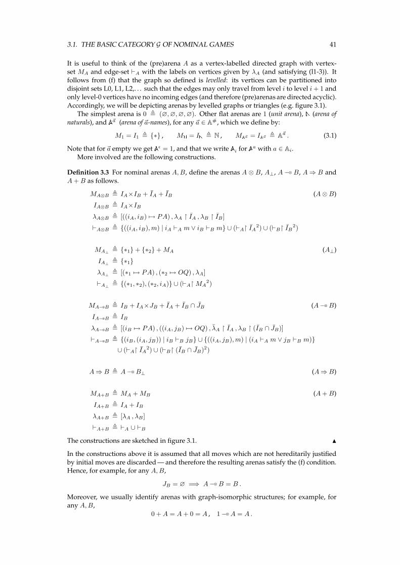
3.1. THE BASIC CATEGORY G OF NOMINAL GAMES 41
It is useful to think of the (pre)arena A as a vertex-labelled directed graph with vertex-set MA and edge-set ⊢A with the labels on vertices given by λA (and satisfying (l1-3)). It
follows from (f) that the graph so defined is levelled: its vertices can be partitioned intodisjoint sets L0, L1, L2,. . . such that the edges may only travel from level i to level i+ 1 and
only level-0 vertices have no incoming edges (and therefore (pre)arenas are directed acyclic).
Accordingly, we will be depicting arenas by levelled graphs or triangles (e.g. figure 3.1).The simplest arena is 0 , (∅,∅,∅,∅). Other flat arenas are 1 (unit arena), N (arena of
naturals), and A~a (arena of ~a-names), for any ~a ∈ A#, which we define by:
M1 = I1 , {∗} , MN = IN , N , MA~a = IA~a , A~a . (3.1)
Note that for ~a empty we get Aǫ = 1, and that we write Ai for Aa with a ∈ Ai.More involved are the following constructions.
Definition 3.3 For nominal arenas A,B, define the arenas A ⊗ B, A⊥, A −−⊗ B, A⇒ B and
A+B as follows.
MA⊗B , IA×IB + IA + IB (A⊗B)
IA⊗B , IA×IB
λA⊗B , [((iA, iB) 7→ PA) , λA ↾ IA , λB ↾ IB ]
⊢A⊗B , {((iA, iB),m) | iA ⊢A m ∨ iB ⊢B m} ∪ (⊢A↾ IA2) ∪ (⊢B↾ IB2)
MA⊥, {∗1} + {∗2} +MA (A⊥)
IA⊥, {∗1}
λA⊥, [(∗1 7→ PA) , (∗2 7→ OQ) , λA]
⊢A⊥, {(∗1, ∗2), (∗2, iA)} ∪ (⊢A↾ MA
2)
MA−−⊗B , IB + IA×JB + IA + IB ∩ JB (A −−⊗ B)
IA−−⊗B , IB
λA−−⊗B , [(iB 7→ PA) , ((iA, jB) 7→ OQ) , λA ↾ IA , λB ↾ (IB ∩ JB)]
⊢A−−⊗B , {(iB, (iA, jB)) | iB ⊢B jB} ∪ {((iA, jB),m) | (iA ⊢A m ∨ jB ⊢B m)}
∪ (⊢A↾ IA2) ∪ (⊢B↾ (IB ∩ JB)2)
A⇒ B , A −−⊗ B⊥ (A⇒B)
MA+B , MA +MB (A+B)
IA+B , IA + IB
λA+B , [λA , λB ]
⊢A+B , ⊢A ∪ ⊢B
The constructions are sketched in figure 3.1. N
In the constructions above it is assumed that all moves which are not hereditarily justified
by initial moves are discarded— and therefore the resulting arenas satisfy the (f) condition.Hence, for example, for any A,B,
JB = ∅ =⇒ A −−⊗ B = B .
Moreover, we usually identify arenas with graph-isomorphic structures; for example, forany A,B,
0 +A = A+ 0 = A , 1 −−⊗ A = A .
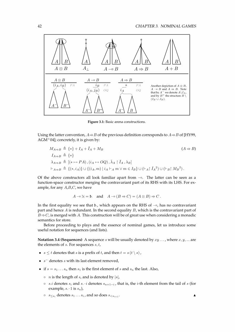
42 CHAPTER 3. NOMINAL GAMES
A B
A⊗B
A
∗∗
A⊥
A B
A −−⊗ B
A B
A⇒B
∗
A B
A+B
A⊗B
(iA, iB) PA
A− B−
A −−⊗ B
iB PA
(iA, jB) OQ
A− B=
A⇒B
∗ PA
iA OQ
A− B
Another depiction ofA⊗ B,A −−⊗ B and A ⇒ B. Notethat byA− we denoteA\IA ,and byB= the structureB \(IB ∪ JB).
Figure 3.1: Basic arena constructions.
Using the latter convention,A⇒B of the previous definition corresponds toA⇒B of [HY99,
AGM+04]; concretely, it is given by:
MA⇒B , {∗} + IA + IA +MB (A⇒B)
IA⇒B , {∗}
λA⇒B , [(∗ 7→ PA) , (iA 7→ OQ) , λA ↾ IA , λB]
⊢A⇒B , {(∗, iA)} ∪ {(iA,m) | iA ⊢A m ∨m ∈ IB} ∪ (⊢A↾ IA2) ∪ (⊢B↾ MB2) .
Of the above constructors all look familiar apart from −−⊗. The latter can be seen as afunction-space constructor merging the contravariant part of its RHS with its LHS. For ex-
ample, for any A,B,C, we have
A −−⊗ N = N and A −−⊗ (B⇒ C) = (A⊗B) ⇒ C .
In the first equality we see that N, which appears on the RHS of −−⊗, has no contravariant
part and hence A is redundant. In the second equality B, which is the contravariant part of
B⇒C, is mergedwithA. This construction will be of great use when considering a monadicsemantics for store.
Before proceeding to plays and the essence of nominal games, let us introduce someuseful notation for sequences (and lists).
Notation 3.4 (Sequences) A sequence swill be usually denoted by xy . . . , where x, y, ... arethe elements of s. For sequences s, t,
• s ≤ t denotes that s is a prefix of t, and then t = s (t \ s) ,
• s− denotes s with its last element removed,
• if s = s1 . . . sn then s1 is the first element of s and sn the last. Also,
◦ n is the length of s, and is denoted by |s|,
◦ s.i denotes si and s.−i denotes sn+1−i , that is, the i-th element from the tail of s (for
example, s.−1 is sn),
◦ s≤sidenotes s1 . . . si , and so does s<si+1 . N
3.1. THE BASIC CATEGORY G OF NOMINAL GAMES 43
We move on to describe how nominal games are played. Given a prearena A, plays of agame consist of sequences of moves from A. These moves are augmented with name-lists
(elements of A#) to the effect of capturing name-environments.
Definition 3.5 Amove-with-names of a prearenaA is a pair, writtenm~a, wherem is a move
of A and ~a is a finite list of distinct names (name-list). N
If x is a move-with-names then its name-list is denoted by nlist(x) and its underlying moveby x ; therefore,
x = xnlist(x) . (3.2)
The above notation is extended to sequences of moves-with-names, so that for such a se-
quence s we write s = snlist(s), where nlist(s) is a list, of length |s|, of lists of names.A justified sequence over a prearena A is a finite sequence s of OP-alternating moves
such that, except for s.1 which is initial, every move s.i has a justification pointer to some
s.j such that j < i and s.j ⊢A s.i ; we say that s.j (explicitly) justifies s.i . A move in s is anopen question if it is a question and there is no answer inside s justified by it.
There are two standard technical conditions that one may want to apply to justified se-quences: well-bracketing and visibility. We say that a justified sequence s iswell-bracketed if
each answer s.i appearing in s is explicitly justified by the last open question in s<s.i , called
the pending question. Seeing questions as opening brackets and answers as closing onesthis condition indeed corresponds to well-bracketing. For visibility, we need to introduce
the notions of Player- andOpponent-view. For a justified sequence s, its P-view psq and its
O-view xsy are defined as follows.
pǫq , ǫ
psxq , psq x if x a P-move
pxq , x if x is initial
psxs′yq , psq xy if y an O-move
expl. justified by x
xǫy , ǫ
xsxy , xsyx if x an O-move
xsxs′yy , xsyxy if y a P-move
expl. justified by x
The visibility condition states that any O-move x in s is justified by a P-move in xs<xy , andany P-move y in s is justified by an O-move in ps<yq. We can now define plays.
Definition 3.6 Let A be a prearena. A legal sequence on A is a sequence of moves-with-
names s such that s is a justified sequence satisfying Visibility and Well-Bracketing.
A legal sequence s is a play if s.1 has empty name-list and s also satisfies the followingName Change Conditions.
(NC1) The name-list of a P-move x in s contains as a prefix the name-list of the move pre-
ceding it. It possibly contains some other names, all of which are fresh for s<x.
(NC2) Any name in the support of a P-move x in s that is fresh for s<x is contained in the
name-list of x.
(NC3) The name-list of a non-initial O-move in s is that of the move explicitly justifying it.
The set of plays on a prearenaA is denoted by PA. N
It is important to observe that plays have strong support, due to the tagging of moves withlists of names (instead of sets of names [AGM+04]). Note also that plays are the ǫ-plays
of [Tze07]. Now, some further notation.
Notation 3.7 (Name-introduction) A name a is introduced (by Player) in a play s, written
a ∈ L(s), whenever there exist consecutive moves yx in s such that x is a P-move anda ∈ nlist(x) \ nlist(y). N
44 CHAPTER 3. NOMINAL GAMES
From plays we move on to strategies. Recall the notion of name-abstraction we introducedin definition 2.7; for any nominal set X and any x ∈ X ,
[x] = {π [x | π ∈ PERM(A)} .
Definition 3.8 Let A be a prearena. A strategy σ on A is a non-empty set of equivalenceclasses [s] of plays in A, satisfying:
• Prefix closure: If [su] ∈ σ then [s] ∈ σ.
• Contingency completeness: If even-length [s] ∈ σ and sx is a play then [sx] ∈ σ.
• Determinacy: If even-length [s1x1], [s2x2] ∈ σ and [s1] = [s2] then [s1x1] = [s2x2].
We write σ : Awhenever σ is a strategy on A. N
By convention, the empty sequence ǫ is a play and hence, by prefix closure and contingency
completeness, all strategies contain [ǫ] and [iA]’s. Note that strategies always have emptysupport because their elements are equivariant support abstractions.
Some basic strategies are the following— note that we give definitions modulo prefix clo-
sure (and recall that ~a′ ⊆ ~a if S(~a′) ⊆ S(~a)).
Definition 3.9 For any ~a′ ⊆ ~a ∈ A#, i, n ∈ N and any arena B, define the following strate-gies.
•bn : 1 B N , { [∗n] } ,
• !B : BB 1 , { [iB ∗] } ,
• ~a~a′ : A~a B A~a′ , { [~a~a′] } ,
• eqi : Ai ⊗ AiB N , { [(a, a) 0] } ∪ { [(a, b) 1] | a# b } ,
• idB : BB B , { [s xx] | |s| even ∧ [s] ∈ idB ∧ s x ∈ PB→B } . N
Note that in general we do not include justification pointers in definitions/expressions ofstrategies (or plays), unless they cannot be easily determined.
3.1.2 Composition
We proceed to composition of plays and strategies. In ordinary games, plays are composedby “parallel composition plus hiding” (v. [AJ94]); in nominal games we need to take some
extra care for fresh names.
Definition 3.10 Let s ∈ PA→B and t ∈ PB→C . We say that:
• s and t are almost composable, s ` t, if s ↾ B = t ↾ B.
• s and t are composable, s ≍ t, if s ` t and, for any s′ ≤ s, t′ ≤ t with s′ ` t′:
(C1) If s′ ends in a (Player) move in A introducing some name a then a# t′ ;dually, if t′ ends in a move in C introducing some name a then a# s′.
(C2) If both s′, t′ end in B and s′ ends in a move introducing some name a then a# t′− ;
dually, if t′ ends in a move introducing some name a then a# s′−. N
The following lemma is taken verbatim from [HY99], adapted from [BDE97].
Lemma 3.11 (Zipper lemma) If s ∈ PA→B and t ∈ PB→C with s ` t then either s ↾ B = t = ǫ,
or s ends in A and t in B, or s ends in B and t in C, or both s and t end in B. �
3.1. THE BASIC CATEGORY G OF NOMINAL GAMES 45
Note that in the sequel wewill use some standard switching condition results (see e.g. [AJM00,HY99]) without further mention. Composable plays are composed as below. Note that jus-
tification pointers inside s ‖ t follow precisely those in s, t. Moreover, we may tag a movemasm(O) (orm(P )) to specify it is an O-move (a P-move).
Definition 3.12 (Play composition) Let s ∈ PA→B and t ∈ PB→C with s ≍ t . Their parallelinteraction s ‖ t and their mix s • t, which returns the final name-list in s ‖ t, are defined by
mutual recursion as below,
ǫ ‖ ǫ , ǫ ǫ • ǫ , ǫ
sm~bA ‖ t , (s ‖ t)m
sm~bA • t
A sm~bA(P ) • t , (s • t), (~b \ nlist(s.−1))
sm~bA(O) • t , ~b′
sm~bB ‖ tm~c
B , (s ‖ t)msm
~bB • tm~c
B
B sm~bB(P ) • tm
~cB(O) , (s • t), (~b \ nlist(s.−1))
sm~bB(O) • tm
~cB(P ) , (s • t), (~c \ nlist(t.−1))
s ‖ tm~cC , (s ‖ t)m
s • tm~cC
C s • tm~cC(P ) , (s • t), (~c \ nlist(t.−1))
s • tm~cC(O) , ~c ′
where~b′ is the name-list ofmA(O)’s justifier inside s ‖ t, and similarly for ~c ′.The composite of s and t is
s ; t , (s ‖ t) ↾ AC .
The set of interaction sequences of A,B,C is defined by:
ISeq(A,B,C) , {s ‖ t | s ∈ PA→B ∧ t ∈ PB→C ∧ s ≍ t} .N
Our aim now is to show that the composite of plays is still a play. The following lemmaexamines the behaviour of name-lists in interactions of plays. In particular, it shows that
condition (NC1) is preserved and that there is no loss of names by composition: although
certain moves may be hidden in composition, their fresh names are propagated inside thename-lists. Note below that a generalised P-move in an interaction sequence of A,B,C is
either a P-move in AC or a move in B.
Lemma 3.13 Let s ≍ t with s ∈ PA→B and t ∈ PB→C .
(a) If s ‖ t ends in a generalised P-movem~b then~b contains as a prefix the name-list of (s ‖ t).−2 . It
possibly contains some other names, all of which are fresh for (s ‖ t)−.
(b) If s ; t ends in a P-move m~b then ~b contains as a prefix the name-list of (s ; t).−2 . It possibly
contains some other names, all of which are fresh for (s ; t)−.
(c) If s ‖ t ends in a movem~b then~b contains as a prefix the name-list of the move explicitly justifying
m~b.
(d) If s = s′m~b ends in A and t in B then~b � s • t,
if s = s′m~b and t = t′m~c end in B then~b � s • t and ~c � s • t,
if s ends in B and t = t′m~c in C then ~c � s • t.
(e) S(s) ∪ S(t) = S(s ‖ t) = S(s ; t) ∪ S(s • t) .
Proof: Part (a) follows from definitions of s ‖ t and s ≍ t, and then part (b) easily follows.For (c) we do induction on |s ‖ t| ; the base case is trivial. Moreover, if s ‖ t ends in an O-move
in AC then the claim trivially holds, by definition of play-composition. So assume that s ‖ t
46 CHAPTER 3. NOMINAL GAMES
ends in a P-move in AB, consider p(s ‖ t) ↾ ABq and take two consecutive moves xy in it. If yis a P-move in AB then xy are consecutive in (s ‖ t) ↾ AB and, by switching condition, they
are also consecutive in s ‖ t ; hence, by part (b) we have that nlist(x) ≤ nlist(y). If y is an O-move inAB and particularly inA then nlist(x) = nlist(y), as x justifies y. Otherwise, y is inB
and justified by x, and, since s ‖ t ends in a P-move in AB, we can apply the IH on s≤y ‖ t≤yand obtain nlist(x) ≤ nlist(y). Therefore, in any subsequence of moves in p(s ‖ t) ↾ ABq thename-list of the last move contains that of the initial move as a prefix. By visibility of s,
the move z justifying (s ‖ t).−1 appears in p(s ‖ t) ↾ ABq, hence nlist(z) ≤ nlist((s ‖ t).−1), asrequired. The case of s ‖ t ending in a P-move in BC is entirely symmetrical.
For (d) we do induction on |s ‖ t|. The base case is encompassed in t being empty, which is
trivial. Now assume s = s′m~b ends in A and t ends in B. If m is an O-move then the claim
follows from the IH applied to s≤x , where x is the justifier ofm~b in s, and the corresponding
subsequence of t, and part (c). Ifm is a P-move then
~b = nlist(s′.−1), (~b \ nlist(s′.−1))IH� s′ • t, (~b \ nlist(s′.−1)) = s • t .
The case of t = t′m~c ending in C is proved similarly. Now, if s = s′m~b and t = t′m~c both
end in B andm a P-move in AB then, reasoning exactly as above, we have that ~b � s • t. If
m is non-initial in B then ms • t is justified by some n~d in s ‖ t , and then, by IH, ~c � ~d , and,
by (c), ~d ≤ s • t , which imply ~c � s • t. The case ofm being a P-move in t is proved similarly.
Now, for (e) we note that the following straightforwardly hold
S(s ‖ t) ⊆ S(s) ∪ S(t) , S(s ; t) ∪ S(s • t) ⊆ S(s ‖ t) .
Moreover, by (d) we obtain S(s) ∪ S(t) ⊆ S(s ‖ t). Finally, we show that S(s ‖ t) ⊆ S(s ; t) ∪S(s • t) by induction on |s ‖ t| . The base case is encompassed in t being empty, which is
trivial. Otherwise, if s = s′m~b ends in A and t ends in B then
S(s ‖ t) = S(s′ ‖ t)∪S(ms • t)IH⊆ S(s′ ; t)∪S(s′ • t)∪S(ms • t)
(∗)
⊆ S(s′ ; t)∪S(s • t)∪S(ms • t) = S(s ; t)
where (∗) holds because if m is a P-move then, by (a), s′ • t ≤ s • t, while if m is an O-move
then S(s′ • t) ⊆ S(s′ ; t). Similarly for the case of t ending in C. For the case of both s = s′m~b
and t = t′m~c ending in B assume wlog thatm~b is a P-move in s. Then
S(m) ⊆ S(m~b) ⊆ S(s′) ∪ S(~b) ⊆ S(s′ ‖ t′) ∪ S(s • t)
and hence
S(s ‖ t) = S(s′ ‖ t′) ∪ S(m) ∪ S(s • t) ⊆ S(s′ ‖ t′) ∪ S(s • t)IH⊆ S(s′ ; t′) ∪ S(s′ • t′) ∪ S(s • t)
(a)
⊆ S(s′ ; t′) ∪ S(s • t) = S(s ; t) ∪ S(s • t)
as required. �
We can now prove the following.
Proposition 3.14 (Plays compose) If s ∈ PA→B and t ∈ PB→C with s ≍ t, then s ; t ∈ PA→C .
Proof: We skip visibility andwell-bracketing, as these follow from ordinary CBV game anal-ysis. It remains to show that the name change conditions hold for s ; t. (NC3) clearly does
by definition, while (NC1) is part (b) of previous lemma.
For (NC2), let s ; t end in some P-movems • t and suppose a ∈ S(ms • t) and a#(s ; t)−. Sup-
pose wlog that s = s′m~b, and so (s ; t)− = s′ ; t. Now, if a# s′ • t then, by part (e) of previous
lemma, a # s′, t and therefore a ∈ ~b , by (NC2) of s. By part (d) then, a ∈ s • t. Otherwise,
a ∈ s′ • t and hence, by part (a), a ∈ s • t. �
We now proceed to composition of strategies. Note that we write σ : A B B if σ is a
strategy on the prearenaA→ B.
3.1. THE BASIC CATEGORY G OF NOMINAL GAMES 47
Definition 3.15 (Strategy composition) For strategies σ : A → B and τ : B → C, theircomposition is defined as
σ ; τ , { [s ; t] | [s] ∈ σ ∧ [t] ∈ τ ∧ s ≍ t } .N
Note that, for any sequence u, if [u] ∈ σ ; τ then u = π [(s ; t) = (π [ s) ;(π [ t) for some
[s] ∈ σ, [t] ∈ τ, s ≍ t and π. Therefore, we can always assume u = s ; t with [s] ∈ σ, [t] ∈ τ
and s ≍ t.
Our next aim is to show that composites of strategies are strategies themselves. Weproceed by first giving two technical lemmata.
Lemma 3.16 For plays s1 ≍ t1 and s2 ≍ t2 , if s1 ‖ t1 = s2 ‖ t2 then s1 = s2 and t1 = t2 . Hence,
if s1 ‖ t1 ≤ s2 ‖ t2 then s1 ≤ s2 and t1 ≤ t2 .
Proof: The first part by easy induction on |s1 ‖ t1| = |s2 ‖ t2|. The second part follows. �
Lemma 3.17 Let σ : A → B and τ : B → C be strategies with [s1], [s2] ∈ σ and [t1], [t2] ∈ τ . If
|s1 ‖ t1| ≤ |s2 ‖ t2| and [s1 ; t1] = [s2 ; t2] then there exists some π such that π [(s1 ‖ t1) ≤ s2 ‖ t2.
Proof: By induction on |s1 ‖ t1|. The base case is encompassed in t1 being empty. In this case,
by switching condition and determinacy of σ, [s1] = [s1 ; t1] = [s2 ; t2] implies that s2 = s′2s′′2
with [s1] = [s′2]. Hence, π [ s1 = s′2 ≤ s2 ‖ t2, for some permutation π, as required.
Now assume that s1, t1 both end in B, say s1 = s′1m~b11 and t1 = t′1m
~c11 . Then, [s1 ; t1] =
[s′1 ; t′1] = [s2 ; t2] so, by IH, there exists some π such that π [ s′1 = s′2 and π [ t′1 = t′2 , with
s2 = s′2s′′2 and t2 = t′2t
′′2 . Moreover, s′′2 , t
′′2 are in B and non-empty; let s′′2 .1 = m
~b22 and
t′′2 .1 = m~c22 and assume wlog thatm2 is a P-move inB → C, so the same holds form1. Then,
by prefix closure, [t′2m~c22 ] ∈ τ , and, as [t′1] = [t′2], we have [t′1m
~c11 ] = [t′2m
~c22 ], so π′ [ t′1m~c1
1 =
t′2m~c22 for some π′. Now, by (C2) we have that (S(m~ci
i ) \ S(t′i)) ∩ S(s′i) = ∅, therefore, by
Strong Support Lemma, there exists some π′′ such that π′′ [m~c11 = m~c2
2 , π′′ [ t′1 = t′2 and
π′′ [ s′1 = s′2 . Moreover, π′′ [ s′1 = s′2 and π′′ [m1 = m2 imply that π′′ [(s′1m~b11 ) = s′2m~b22 .
Hence, π′′ [(s1 ‖ t1) ≤ s2 ‖ t2 , as required.
Now assume s1 ends in A and t1 in B, say s1 = s′1m~b11 . Then, [s1 ; t1] = [s2 ; t2] implies
that s2 = s′2m~b22 s
′′2 and t2 = t′2t
′′2 with [s1 ; t1] = [s′2m
~b22 ; t′2] , m2 in A and s′′2 , t
′′2 in B. Then,
[s′1 ; t1] = [s′2 ; t′2], and, by IH, there exists a π such that π [ s′1 = s′21 , π [ t1 = t′21 , s′2 = s′21s
′22 ,
t′2 = t′21t′22 and s′22, t
′22 in B.
If m1 is an O-move then, by switching condition, s′1 ends in A, and so does s′2 . Hence,
s′22 = t′22 = ǫ and thus π [ s′1 = s′2 , π [ t1 = t′2 . Now, from [s1 ; t1] = [s′2m~b22 ; t′2] we have
π′ [(s1 ; t1) = s′2m~b22 ; t′2 , some π′. Taking π′′ = π−1 ◦ π′ we have that π′′ [(s′1 ; t1) = s′1 ; t1
and therefore, by strong support, π′′ fixes all elements in S(s′1 ; t1)lm 3.13
= S(s′1) ∪ S(t1), thusπ′′ [ s′1 = s′1, ∴ π′ [ s′1 = π [ s′1 = s′2 , and similarly π′ [ t1 = t′2 . Hence, π′ [(s1 ‖ t1) =
π′ [ s1 ‖ π′ [ t1 = s′2m~b22 ‖ t′2 ≤ s2 ‖ t2 .
If m1 is a P-move then, by prefix-closure, [s′1m~b11 ], [s′21(s
′22m
~b22 ).1] ∈ σ and [s′1] = [s′21], thus,
by determinacy of σ, [s′1m~b11 ] = [s′21(s
′22m
~b22 ).1] so s′22 = t′22 = ǫ and π′ [(s′1m~b11 ) = s′2m
~b22 ,
some π′. Because of (C1), we can now apply the Strong Support Lemma and obtain a π′′
such that π′′ [(s1 ‖ t1) = s′2m~b22 ‖ t′2 ≤ s2 ‖ t2 .
The case of s1 ending in B and t1 in C is entirely symmetrical. �
Proposition 3.18 (Strategies compose) If σ : A → B and τ : B → C are strategies then so is
σ ; τ .
Proof: By definition and proposition 3.14, σ ; τ contains equivalence classes of plays. We
need also check the following.
• Prefix-closure: Assume [um~b] ∈ σ ; τ . Then, by prefix closure of σ, τ , there exist s, t not
48 CHAPTER 3. NOMINAL GAMES
both ending in B and such that s ; t = um~b, [s] ∈ σ, [t] ∈ τ . Now, assume wlog that m is in
C, so t = t′m~b′ and s ; t = (s ; t′)m
~b. By prefix-closure of τ , [t′] ∈ τ , ∴ [s ; t′] ∈ σ ; τ .
• Contingency completeness: Assume [u] ∈ σ ; τ is even-length and um~b a play. Then
u = s ; t, some [s] ∈ σ, [t] ∈ τ . Suppose wlog that m is in A. As it is an O-move, u is either
empty or it ends in a P-move in A. The former case is trivial. In the latter case, taking ~b′ to
be the name-list ofm’s justifier inside s, sm~b′ is a play: visibility and well-bracketing follow
from ordinary CBV-game analysis,2while name change conditions clearly hold. Moreover,
[sm~b′ ; t] = [um
~b] ∈ σ ; τ , as required.
• Determinacy: Assume even-length [u1x1], [u2x2] ∈ σ ; τ with [u1] = [u2], say uixi = si ; ti,[si] ∈ σ and [ti] ∈ τ , i = 1, 2 . By prefix-closure of σ, τ we may assume that si, ti don’t both
end in B, for i = 1, 2.
If si end in A then si = s′in~bi
i and si ; ti = (s′i ; ti)n~b′ii , i = 1, 2 . Now, [s′1 ; t1] = [u1] =
[u2] = [s′2 ; t2], so, by lemma 3.17 and assuming wlog that |s′1 ‖ t1| ≤ |s′2 ‖ t2|, we have
π [(s′1 ‖ t1) ≤ (s′2 ‖ t2), ∴ π [ s′1 ≤ s′2 , say s′2 = s′′2s
′′′2 with s′′2 = π [ s′1 and s′′′2 in B. Then
[s′′2 ] = [s′1], ∴ [s′′2(s′′′2 n~b22 ).1] = [s′1n
~b11 ], by determinacy of σ, and hence |s′′′2 | = 0, s′2 = π [ s′1
and t2 = π [ t1 . Moreover, π′ [ s′1n~b11 = s′2n~b22 , some permutation π′. Now we can apply the
Strong Support Lemma, as (C1) implies (S(n~bi
i ) \ S(s′i)) ∩ S(ti) = ∅. Hence, there exists a
permutation π′′ such that π′′ [ s1 = s2 and π′′ [ t1 = t2, ∴ [s1 ; t1] = [s2 ; t2] , as required.If si end in B and ti in C, then work similarly as above. These are, in fact, the only cases we
need to check. Because if, say, s2, t1 end in B, s1 in A and t2 in C then t1, s2 end in P-movesand [s−1 ; t1] = [s2 ; t−2 ] implies that s−1 , t
−2 end in O-moves in B. If, say, |s−1 ‖ t1| ≤ |s2 ‖ t
−2 |
then we have, by lemma 3.17, π [ s−1 ≤ s2 , some permutation π. So if π [ s−1 = s′2 and
s2 = s′2s′′2 , determinacy of σ dictates that s′′2 .1 be in A, to |s1 ; t1| = |s2 ; t2| and s2 ; t2 end-
ing in C. �
In the following remark we examine the previous proof closer in order to identify where
exactly strong support is needed. This analysis provides a view on the reasons for which
the nominal games model of [AGM+04] is flawed. In fact, we provide specific counterex-amples for needed properties which fail in that model.
Remark 3.19 (The need for strong support) The nominal games presented here differ fromthose of [AGM+04] crucially in one aspect: the requirement for strong support. In [AGM+04]
plays are weakly supported since local state is modelled by finite sets of names, so a move-with-names is a move attached with a finite set of names (hence, no strong support), and
other definitions differ accordingly. The problem is that thus determinacy is not preserved
by strategy composition: information separating freshly created names may be hidden bycomposition and hence a composite strategy may break determinacy by distinguishing be-
tween composite plays that are equivalent.In particular, in the proof of determinacy above we first derived from [s′1 ; t1] = [s′2 ; t2]
that there exists some π so that π [ s′1 = s2 and π [ t1 = t2, by appealing to lemma 3.17; in
the proof of that lemma, the Strong Support Lemma needs to be used several times. In fact,the statement
|s′1 ‖ t1| = |s′2 ‖ t2| ∧ [s′1 ; t1] = [s′2 ; t2] =⇒ ∃π. π [ s′1 = s′2 ∧ π [ t1 = t2
does not hold in a weak support setting such as that of [AGM+04]. For take some i ∈ ω and
2Visibility holds because xsy = xuy. For well-bracketing, if m is an Answer then its justifier, say n, is in A, and n
is the pending Question of u. Now, because u ↾ A = s ↾ A, if the pending-Q of s is in A then it is n. Otherwise, thepending-Q of s is some n′ in B, and s = s1ns2n′s3. Since s satisfies well-bracketing all Answers in s3 are justifiedby Q’s within s3, and since n′ is the pending-Q all Q’s in s3 are answered. Hence, s3 is even-length and n′ is aP-move. Moreover, all A’s in s3 ↾ A are justified within s3 ↾ A, so s3 ↾ A is also even-length,to the switchingcondition
3.1. THE BASIC CATEGORY G OF NOMINAL GAMES 49
consider the following AGMOS-strategies.
σ : 1B Ai , { [∗ a{a,b}] | a 6= b ∈ Ai } ,
τ : AiB Ai ⇒ Ai , { [a ∗ c a] | a, c ∈ Ai } .(3.19:A)
Then
[∗ a{a,b} ; a ∗ b] = [∗ ∗{a,b} b{a,b}] = [∗ ∗{a,b} a{a,b}] = [∗ a{a,b} ;a ∗ a] ,
yet for no π dowe have π [(∗ a{a,b}) = ∗ a{a,b} and π [(a∗ b) = a∗ a . As a result, determinacy
fails for σ ; τ since both [∗ ∗{a,b} b{a,b}a{a,b}], [∗ ∗{a,b} a{a,b}a{a,b}] ∈ σ ; τ .Another point where we used the Strong Support Lemma in the proof of determinacy
was in showing (the dual of):
∃π, π′. π [(s1, t′1) = (s2, t′2) ∧ π′ [ t′1n~b11 = t′2n
~b22 =⇒ ∃π′′. π′′ [(s1, t′1n~b11 ) = (s2, t
′2n~b22 )
i.e. [s1, t′1] = [s2, t
′2] ∧ [t′1n
~b11 ] = [t′2n
~b22 ] =⇒ [s1, t
′1n~b11 ] = [s2, t
′2n~b22 ] .
The above statement does not hold for AGMOS-games. To show this, we need to introduce3
the flat arena Ai⊙Ai withMAi⊙A
i, P2(Ai) (the set of 2-element subsets of Ai). This is not a
legal arena in our setting, since its moves are not strongly supported, but it is in the AGMOS
setting. Consider the following strategies.
σ : Ai ⊗ AiB Ai⊙Ai , { [(a, b) {a, b}] | a 6= b ∈ Ai }
τ : Ai⊙AiB Ai , { [{a, b} a] | a 6= b ∈ Ai }(3.19:B)
We have that [(a, b) {a, b}, {a, b}] = [(a, b) {a, b}, {a, b}] and [{a, b} a] = [{a, b} b] , yet
[(a, b) {a, b}, {a, b} a] 6= [(a, b) {a, b}, {a, b} b] .
In fact, determinacy is broken since [(a, b) a], [(a, b) b] ∈ σ ; τ .
Our final task in this section is to show that composition of strategies is associative. Note
first that by lemma 3.13, part (a), if s ≍ t then the name-list of (s ‖ t).−1 contains as a prefixthat of (s ; t).−1. This allows for the following definition.
Definition 3.20 Let s ∈ PA→B, t ∈ PB→C with s ≍ t . If s ; t ends in a movem~b, define
s ◦ t , s • t \~b ,
that is, s • t = ~b, s ◦ t. N
Note in particular that if s ; t and s ‖ t end in the same move then s ◦ t = ǫ. Now we extend
parallel interaction to triples of plays.
Definition 3.21 Let s ∈ PA→B , t ∈ PB→C and u ∈ PC→D with (s ; t) ≍ u and s ≍ (t ;u).
3In the AGMOS setting, plays with non-empty initial local state are allowed. Hence, we could have used to thesame effect the {a, b}-strategies:
σ : Ai ⊗ AiB 1 , { [(a, b){a,b}∗{a,b}]{a,b} } , τ : 1B Ai , { [∗{a,b}a{a,b}
]{a,b} } .
50 CHAPTER 3. NOMINAL GAMES
Define s ‖ t ‖ u and s • t •u as follows,
ǫ ‖ ǫ ‖ ǫ , ǫ ǫ • ǫ • ǫ , ǫ
sm~bA ‖ t ‖ u , (s ‖ t ‖u)m
sm~bA • t • u
A sm~bA(P ) • t • u , (s • t •u), (~b \ nlist(s.−1))
sm~bA(O) • t • u , ~b′
sm~bB ‖ tm~c
B ‖ u , (s ‖ t ‖u)msm
~bB • tm~c
B • uB sm
~bB(P ) • tm
~cB(O) • u , (s • t •u), (~b \ nlist(s.−1))
sm~bB(O) • tm
~cB(P ) • u , (s • t •u), (~c \ nlist(t.−1))
s ‖ tm~cC ‖ um
~dC , (s ‖ t ‖u)m
s • tm~cC • um
~dC
C s • tm~cC(P ) • um
~dC(O) , (s • t •u), (~c \ nlist(t.−1))
s • tm~cC(O) • um
~dC(P ) , (s • t •u), (~d \ nlist(u.−1))
s ‖ t ‖um~dD , (s ‖ t ‖u)m
s • t •um~dD
D s • t •um~dD(P ) , (s • t •u), (~d \ nlist(u.−1))
s • t •um~cD(O) , ~d ′
where~b′ is the name-list ofmA(O)’s justifier inside s ‖ t ‖u, and similarly for ~d ′. N
Note that the conditions s ≍ t, t ≍ u, (s ; t) ≍ u and s ≍ (t ;u) in the above definition indeedimply that exactly one of the following is the case: s ends in A, or s, t end in B, or t, u end in
C, or u ends in D. We can now show the following.
Lemma 3.22 If s1 ∈ PA1→A2 , s2 ∈ PA2→A3 and s3 ∈ PA3→A4 with (s1 ; s2) ≍ s3 and s1 ≍(s2 ; s3) then
(s1; s2); s3 = (s1 ‖ s2 ‖ s3) ↾ A1A4 = s1 ;(s2 ; s3) ,
(s1; s2) • s3, s1 ◦ s2 = s1 • s2 • s3 = s1 •(s2 ; s3), s2 ◦ s3 .
Proof: By induction on k = |s1 ‖ s2 ‖ s3|. The case of k = 0 is trivial; otherwise:
# (s1m~bA1
; s2) ; s3 = ((s1 ; s2) ; s3)m~b′
A1
IH= ((s1 ‖ s2 ‖ s3)m
~b′
A1) ↾ A1A4 , where~b′ = (s1m
~bA1
; s2) • s3.
Thus, it suffices to show that (s1m~bA1
; s2) • s3 = s1m~bA1
• s2 • s3 . Since s1m~bA1
◦ s2 = ǫ, that
would also imply s1m~bA1
• s2 • s3 = (s1m~bA1
; s2) • s3 , s1m~bA1
◦ s2 . Now, if mA1 an O-move
then the assertion holds by definition. On the other hand, if mA1 a P-move then ~b′ =
(s1 ; s2) • s3 ,(~b′′ \ nlist((s1 ; s2).−1)) and~b′′ = s1 • s2 ,(~b \ nlist(s1.−1)) , while s1m~bA1
• s2 • s3 =
(s1 • s2 • s3) ,(~b \ nlist(s1.−1)) . By IH, s1 • s2 • s3 = (s1 ; s2) • s3 , s1 ◦ s2 , thus
~b′ = (s1 ; s2) • s3 ,(~b′ \ nlist((s1 ; s2).−1))
= (s1 ; s2) • s3 ,((s1 • s2 ,(~b \ nlist(s1.−1))) \ nlist((s1 ; s2).−1))
= (s1 ; s2) • s3 ,(s1 • s2 \ nlist((s1 ; s2).−1)) ,(~b \ nlist(s1.−1))
= (s1 ; s2) • s3 , s1 ◦ s2 ,(~b \ nlist(s1.−1)) = s1m~bA1
• s2 • s3 .
Also, s1m~bA1
;(s2 ; s3) = (s1 ;(s2 ; s3))m~b′
A1
IH= ((s1 ‖ s2 ‖ s3)m
~b′
A1) ↾ A1A4 , with~b′ = s1m
~bA1
•(s2 ; s3) .
Note that s2 ‖ s3 necessarily ends in a P-move in A2 and therefore s2 ◦ s3 = ǫ. Now, it suf-
fices to show that s1m~bA1
•(s2 ; s3) = s1m~bA1
• s2 • s3 ; that would also imply s1m~bA1
• s2 • s3 =
s1m~bA1
•(s2 ; s3) , s2 ◦ s3 . If mA1 an O-move then the assertion holds by definition. If a P-
move then~b′ = s1 •(s2 ; s3) ,(~b \ nlist(s1.−1)), which is what required, because of the IH.
# (s1m~bA2
; s2m~cA2
) ; s3 = ((s1 ; s2) ; s3)IH= (s1 ‖ s2 ‖ s3) ↾ A1A4
IH= (s1 ;(s2 ; s3)) = (s1m
~bA2
;(s2m~cA2
; s3)).
3.1. THE BASIC CATEGORY G OF NOMINAL GAMES 51
IfmA2 is a P-move in A1 → A2 then s2 ‖ s3 ends in a P-move in A2 , so s2 ◦ s3 = ǫ, and
s1m~bA2
◦ s2m~cA2
= s1m~bA2
• s2m~cA2
\ nlist((s1m~bA2
; s2m~cA2
).−1)
= (s1 • s2 ,(~b \ nlist(s1.−1))) \ nlist((s1 ; s2).−1)
= (s1 • s2 \ nlist((s1 ; s2).−1)) ,(~b \ nlist(s1.−1))
= s1 ◦ s2 ,(~b \ nlist((s1 ; s2).−1)) ,
(s1m~bA2
; s2m~cA2
) • s3 ,(s1m~bA2
◦ s2m~cA2
) = (s1 ; s2) • s3 , s1 ◦ s2 ,(~b \ nlist(s1.−1))
IH= s1 • s2 • s3 ,(~b \ nlist(s1.−1)) = s1m
~bA2
• s2m~cA2
• s3
s1m~bA2
•(s2m~cA2
; s3) , s2m~cA2
◦ s3 = s1m~bA2
•(s2 ; s3)m~c′
A2= s1 •(s2 ; s3) ,(~b \ nlist(s1.−1))
IH=
s2 ◦ s3=ǫs1 • s2 • s3 ,(~b \ nlist(s1.−1)) = s1m
~bA2
• s2m~cA2
• s3 .
The case ofmA2 being a P-move in A2 → A3 is entirely symmetrical.
# The other cases are shown similarly. �
The two conditions in the previous lemma are sometimes equivalent.
Lemma 3.23 If s1 ∈ PA1→A2 , s2 ∈ PA2→A3 , s3 ∈ PA3→A4 and either s1 ends in A1 or s3 in A4
then
(s1 ; s2) ≍ s3 ⇐⇒ s1 ≍ (s2 ; s3)
Proof: We show only the left-to-right implication; the other is shown similarly. Note thatwe may use lemma 3.13 without further mention.
Assume (s1 ; s2) ≍ s3 . It is easy to see that s1 ≍ s2 ` s3 , so, using the assumption for
A1A4, not both s1, s2 end in A2 nor both s2, s3 end in A3 . Now let s′2 ≤ s2 and s′3 ≤ s3 withs′2 ` s′3 . If s
′2.−1 introduces a (and s′3 ends in A3) then, if this introduction occurs in A3 then
(s′1 ; s′2).−1 introduces a, for relevant s′1 ≤ s1 , so a # s′−3 . If the introduction occurs in A2
then there exist least prefixes s′′1 ≤ s1 and s′2 ≤ s′′2 ≤ s2 such that |s′′1 ; s′′2 | = |s′1 ; s′2| + 1 and
(s′′1 ; s′′2).−1 introduces a. Hence, a# s′3 . On the other hand, if s′3.−1 introduces a and s′2 ends
in A3 then, taking relevant s′1 ≤ s1 , either a# s′1 ; s′2 or a# (s′1 ; s′2)−, according to whether
a being introduced in A4 or in A3 , which implies a# s′2 or a# s′−2 . Hence, s2 ≍ s3 .
It is not difficult to see that s1 ` (s2 ; s3) . Now let s′i ≤ si , i = 1, 2, 3 , with s′1 ` (s′2 ; s′3) and
s′2, s′3 not both ending in A3 , so (s′1 ; s′2) ` s′3 and thus (s′1 ; s′2) ≍ s′3 . Assume s′1.−1 intro-
duces a name a and s′2 ; s′3 ends in A2 . If the introduction occurs in A1 then (s′1 ; s′2).−1 also
introduces a, so a# s′2, s′3, ∴ a# (s′2 ; s′3) . If it occurs in A2 then there exist least prefixes
s′1 ≤ s′′1 ≤ s1 and s′2 ≤ s′′2 ≤ s2 such that |s′′1 ; s′′2 | = |s′1 ; s′2| + 1 and (s′′1 ; s′′2).−1 introduces
a. Hence, a# s′3 and, as a# s′−2 , a# (s′2 ; s′3)−. Now assume (s′2 ; s′3)−1 introduces a and s′1
ends in A2 . If the introduction occurs in A2 then a is introduced by s′′2 .−1, some relevants′′2 ≤ s′2 , or by s
′′3 .−1, some relevant s′′3 ≤ s′3 . In the former case, s′1 ≍ s′2 implies a# s′−1 . In
the latter, a is introduced in A3 by s′′3 .−1 and, taking s′′2 ≤ s′2 with s′′2 ≍ s′′3 , we have s′−1 ≍ s′′2and a # (s′−1 ; s′′2)−, so a # s′−1 . If the introduction occurs in A4 then we follow a similar
reasoning. �
With the results we have gathered we obtain a category of nominal games.
Proposition 3.24 For any σ : AB B, idA ;σ = σ = σ ;idB .
Moreover, for any σ1 : A′ B A and σ3 : BB B′, (σ1 ;σ) ;σ3 = σ1 ;(σ ;σ3) .
Proof: The first part is straightforward. For the second part, take some [u] ∈ (σ1 ;σ) ;σ3. By
prefix-closure we may assume that u = s ; s3 with s and s3 not both ending in B, and that
52 CHAPTER 3. NOMINAL GAMES
s = s1 ; s2 with s1 and s2 not both ending in A, so
u = (s1 ; s2) ; s3 ∧ [s1] ∈ σ1 ∧ [s2] ∈ σ ∧ [s3] ∈ σ3 ∧ (s1 ; s2) ≍ s3
∴ u = s1 ;(s2 ; s3) ∧ [s1] ∈ σ1 ∧ [s2] ∈ σ ∧ [s3] ∈ σ3 ∧ s1 ≍ (s2 ; s3)
∴ [u] ∈ σ1 ;(σ ;σ3)
Thus (σ1 ;σ2) ;σ3 ⊆ σ1 ;(σ2 ;σ3) and similarly the other inclusion. �
Definition 3.25 (Category of nominal games) G is the category having nominal arenas asobjects and nominal strategies as arrows. N
3.1.3 Arena and strategy orders in G
G is the raw material from which several subcategories of nominal games will emerge. Still
though there is structure in G which will be inherited to the refined subcategories we will
consider later on. In particular, we will consider orderings for arenas and strategies, thelatter enriching G over Cpo.4
Strategies are (nominal) sets and hence ordered by the subset relation.
Definition 3.26 (Strategy order) For any arenas A,B and each σ, τ ∈ G(A,B) define:
σ ⊑ τ△
⇐⇒ σ ⊆ τ .
For each ⊑-increasing sequence (σi)i∈ω take⊔
i σi ,⋃
i σi. N
It is easy to see that each such a⊔
i σi is indeed a strategy: prefix closure, contingencycompleteness and determinacy easily follow from the fact that the sequences we consider
are⊑-increasing. Hence, each G(A,B) is a cpo with least element the empty strategy (i.e. thestrategy containing only [ǫ] and [iA]’s). More than that, these cpo’s enrich G.
Proposition 3.27 G is Cpo-enriched wrt ⊑.
Proof: Enrichment amounts to showing the following straightforward assertions.
σ ⊑ σ′ ∧ τ ⊑ τ ′ =⇒ σ ; τ ⊑ σ′ ; τ ′
(σi)i∈ω an ω-chain =⇒ (⊔
i∈ω
σi) ; τ ⊑⊔
i∈ω
(σi ; τ)
(τi)i∈ω an ω-chain =⇒ σ ;(⊔
i∈ω
τi) ⊑⊔
i∈ω
(σ ; τi)�
On the other hand, arenas are tuples and hence also ordered by a ‘subset relation’.
Definition 3.28 (Arena order) For any A,B ∈ Ob(G) define
A E B ⇐⇒ MA ⊆MB ∧ IA ⊆ IB ∧ λA ⊆ λB ∧ ⊢A ⊆ ⊢B ,
and for any E-increasing sequence (Ai)i∈ω define⊔
i∈ω
Ai ,⋃
i∈ω
Ai .
If A E B then we can define an embedding-projection pair of arrows by setting
inclA,B : AB B , {[s] | s ∈ PA→B ∧ ([s] ∈ idA ∨ (odd(|s|) ∧ [s−] ∈ idA))} ,
projB,A : BB A , {[s] | s ∈ PB→A ∧ ([s] ∈ idA ∨ (odd(|s|) ∧ [s−] ∈ idA))} .
N4By cpo we mean a partially ordered set with least element and least upper bounds for increasing ω-sequences.
Cpo is the category of cpos and continuous functions.
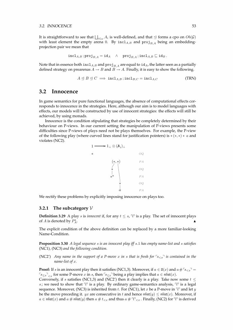
3.2. INNOCENCE 53
It is straightforward to see that⊔
i∈ω Ai is well-defined, and that E forms a cpo on Ob(G)
with least element the empty arena 0. By inclA,B and projB,A being an embedding-
projection pair we mean that
inclA,B ; projB,A = idA ∧ projB,A ; inclA,B ⊑ idB .
Note that in essence both inclA,B and projB,A are equal to idA, the latter seen as a partially
defined strategy on prearenasA→ B and B → A. Finally, it is easy to show the following.
A E B E C =⇒ inclA,B ; inclB,C = inclA,C (TRN)
3.2 Innocence
In game semantics for pure functional languages, the absence of computational effects cor-responds to innocence in the strategies. Here, although our aim is to model languages with
effects, our models will be constructed by use of innocent strategies: the effects will still beachieved, by using monads.
Innocence is the condition stipulating that strategies be completely determined by their
behaviour on P-views. In our current setting the manipulation of P-views presents somedifficulties since P-views of plays need not be plays themselves. For example, the P-view
of the following play (where curved lines stand for justification pointers) is ∗ (∗, ∗) ∗ a andviolates (NC2).
1 // 1⊥ ⊗ (Ai)⊥∗ OQ
(∗, ∗) PA
∗ OQ
∗a PA
∗ OQ
a PA
We rectify these problems by explicitly imposing innocence on plays too.
3.2.1 The subcategory V
Definition 3.29 A play s is innocent if, for any t ≤ s, ptq is a play. The set of innocent playsof A is denoted by P i
A. N
The explicit condition of the above definition can be replaced by a more familiar-looking
Name-Condition.
Proposition 3.30 A legal sequence s is an innocent play iff s.1 has empty name-list and s satisfies
(NC1), (NC3) and the following condition.
(NC2’) Any name in the support of a P-move x in s that is fresh for ps<xq is contained in thename-list of x.
Proof: If s is an innocent play then it satisfies (NC1,3). Moreover, if a ∈ S(x) and a#ps<xq =
ps≤xq<x for some P-move x in s, then ps≤xq being a play implies that a ∈ nlist(x).
Conversely, if s satisfies (NC1,3) and (NC2’) then it clearly is a play. Take now some t ≤s ; we need to show that ptq is a play. By ordinary game-semantics analysis, ptq is a legal
sequence. Moreover, (NC3) is inherited from t. For (NC1), let x be a P-move in ptq and let y
be the move preceding it. yx are consecutive in t and hence nlist(y) ≤ nlist(x). Moreover, ifa ∈ nlist(x) and a# nlist(y) then a# t<x and thus a# ptq<x . Finally, (NC2) for ptq is derived
54 CHAPTER 3. NOMINAL GAMES
from (NC2’) for t. �
Summarising:
A legal sequence s is an innocent play if s.1 has empty name-list and s also satisfiesthe following Name Change Conditions:
(NC1) The name-list of a P-move x in s contains as a prefix the name-list of the
move preceding it. It possibly contains some other names, all of which arefresh for s<x.
(NC2’) Any name in the support of a P-move x in s that is fresh for ps<xq is con-
tained in the name-list of x.
(NC3) The name-list of a non-initial O-move in s is that of the P-move explicitly
justifying it.
Figure 3.2: Definition of innocent play.
We can obtain the following characterisation of name-introduction in innocent plays.
Proposition 3.31 (Name-introduction) Let s be an innocent play. A name a is introduced byPlayer in s iff there exists a P-move x in s such that a ∈ S(x) and a# ps<xq.
Proof: If a is introduced by a P-move x in s then a ∈ nlist(x) and a# nlist(s<x.−1), hence, by
(NC1), a# s<x so a# ps<xq.Conversely, if a ∈ S(x) and a # ps<xq then by (NC2’) we get a ∈ nlist(x), while a # ps<xqimplies a# nlist(s<x.−1). �
We proceed to show that innocent plays are closed under composition. First, we defineP-views of interaction sequences. Recall that in an interaction sequence of A,B,C a move
is a generalised P-move if it is either a P-move in AC or a move in B. The component of a
generalised P-move x is AB if x represents a P-move in component AB, otherwise it is BC.Similar things apply for generalised O-moves.
Definition 3.32 Let w ∈ ISeq(A,B,C) . Define its P-view pwq by recursion as follows.
pǫq , ǫ
pxq , x if x an initial move in A,
pwxq , pwqx if x a generalised P-move,
pwxw′yq , pwqxy if y an O-move in AC justified by x.N
We will need the following results, which are taken verbatim from [McC00].
Lemma 3.33
(a) Let s be a legal sequence and y be a P-move. If psq y is legal then sy is.
(b) Let w ∈ ISeq(A,B,C) and let x be a generalised O-move of w with component X . If x is not
initial in X , write y for its justifier and y′ for the move immediately before y. Then,
(1) If x is not initial in X then y′ is a generalised O-move with componentX .
(2) If x is not initial in X and appears in pwq then both y and y′ appear in pwq.
(3) If x appears in pwq then ppwq≤x ↾ Xq = pw≤x ↾ Xq. �
3.2. INNOCENCE 55
Wewill also need the following lemmata. Note that if x is amove in s and s ‖ t = (s<x ‖ t′)xw
then we say that x appears in s ‖ t as x.
Lemma 3.34 If s1, s2 ∈ PA→B , t1, t2 ∈ PB→C and si ‖ ti end in a generalised O-move x,
(a) if x has component AB then p(s1 ‖ t1) ↾ ABq = p(s2 ‖ t2) ↾ ABq =⇒ ps1q = ps2q ,
(b) if x has component BC then p(s1 ‖ t1) ↾ BCq = p(s2 ‖ t2) ↾ BCq =⇒ pt1q = pt2q .
Proof: We show (a) by induction on |s1| ≥ 1, and (b) is proved similarly. If |s1| = 1 then
|s2| = 1 and, clearly, s1 = s2. If s1 = s′1n~b1s′′1m
~b1 , with m an O-move in A justified by
n, then s2 = s′2n~b2s′′2m
~b2 . Moreover, ti = t′it′′i , i = 1, 2, and si ‖ ti = (s′i ‖ t
′i)n
~b′iuim~b′i ,
with ~b′i = (s′i • t′i)(~bi \ nlist(s′i.−1)), and hence p(s1 ‖ t1) ↾ ABq = p(s2 ‖ t2) ↾ ABq implies that
p(s′1 ‖ t′1) ↾ ABq = p(s′2 ‖ t
′2) ↾ ABq, s′1 • t
′1 = s′2 • t
′2 and
~b′1 = ~b′2. By IH, ps′1q = ps′2q and~b1 = ~b2 ,
as~bi = nlist(s′i.−1)(~b′i \ nlist(s′1 • t′i)) . Thus, ps1q = ps2q.
If s1 = s′1n~b1s′′1m
~b1 , with m an O-move in B justified by n, then s2 = s′2n~b2s′′2m
~b2 , and we
work similarly to the previous case. �
Lemma 3.35 Let s ∈ PA→B , t ∈ PB→C be innocent and s ≍ t . Then,
(a) there exist innocent s′ ∈ PA→B , t′ ∈ PB→C with s′ ≍ t′ such that ps ‖ tq = s′ ‖ t′ ,
(b) S(ps ‖ tq) = S(ps ; tq) ∪ S(s • t) ,
(c) if s ‖ t ends in a generalised O-move inAB and x appears in psq then x appears in ps ‖ tq as somex; similarly for BC and t.
Proof: For (a), we do induction on |s ‖ t| ≥ 1. The base case is trivial. Otherwise, let s ‖ t beending in an O-move in AC, say wlog in a move x in A. Then s = s1s2x and t = t1t2 , with
x justified by s1.−1, so ps ‖ tq = ps1 ‖ t1qx′. By IH, there exist s′, t′ such that ps1 ‖ t1q = s′ ‖ t′.Now, it is easy to see that s′x is a play and that ps ‖ tq = s′x ‖ t′.If s ‖ t ends in a P-move inAC, say wlog in a move x inA, then s = s−x and s ‖ t = (s− ‖ t)x′.By IH, ps− ‖ tq = s′ ‖ t′, some s′, t′. Since s− ‖ t ends in a generalised O-move, we have
that p(s− ‖ t) ↾ ABq = pps− ‖ tq ↾ ABq = p(s′ ‖ t′) ↾ ABq, so ps−q = ps′q. Hence, ps′q x is a
play. We have that s′x is a legal sequence and also that it satisfies (NC2’-3). For (NC1), ifb ∈ (nlist(x)\nlist(s′.−1)) then b ∈ (nlist(x)\nlist(s−.−1)), so b# s−, t, ∴ b#ps− ‖ tq = s′ ‖ t′,∴ b# s′. Hence, ps ‖ tq = s′x ‖ t.If s ‖ t ends in a B-move then we combine the treatments of the two cases above.
For (b), we have that S(ps ‖ tq) = S(s′ ‖ t′) = S(s′ ; t′) ∪ S(s′ • t′) = S(ps ; tq) ∪ S(s • t) .For (c), we have that ps ‖ tq = s′ ‖ t′ and x appears in s′, as p(s ‖ t) ↾ ABq = pps ‖ tq ↾ ABq =
p(s′ ‖ t′) ↾ ABq, ∴ psq = ps′q. �
Now we can show the following.
Proposition 3.36 If s ∈ PA→B , t ∈ PB→C are innocent and s ≍ t then s ; t is innocent.
Proof: Suppose s ; t is not innocent and let u be its least prefix manifesting this, so puq is not
a play. Then puq doesn’t satisfy (NC2). By leastness, u = u′m~b ,m a P-move and there exists
some a such that a ∈ S(m), a ∈ S(u′) but a#~b, pu′q.Supposem is in A, so s = s′m
~b′s′′, t = t′t′′ and u′ = s′ ; t′ . ~b′ is contained in~b , so a#~b′ and
hence a ∈ S(ps′q), since s is innocent. Now, s′ ‖ t′ O-ends in AB and~b contains s′ • t′, so
S(ps′q) ⊆ S(p(s′ ‖ t′) ↾ ABq) = S(pps′ ‖ t′q ↾ ABq) ⊆ S(ps′ ‖ t′q ↾ AB) ⊆ S(ps′ ‖ t′q)
= S(ps′ ; t′q) ∪ S(s′ • t′) ⊆ S(ps′ ; t′q) ∪ S(~b) .
Thus, a ∈ S(ps′ ; t′q) or a ∈ ~b, . Similarly ifm is in C. �
We move on to innocent strategies.
56 CHAPTER 3. NOMINAL GAMES
Definition 3.37 A strategy σ is innocent if [s] ∈ σ implies that s is innocent, and if even-length [s1x1] ∈ σ and odd-length [s2] ∈ σ have [ps1q] = [ps2q] then there exists x2 such that
[s2x2] ∈ σ and [ps1x1q] = [ps2x2q] . N
Some nice properties of innocent strategies are the following.
Lemma 3.38 Let σ be an innocent strategy.
(1) If [s] ∈ σ then [psq] ∈ σ.
(2) If sy is an even-length innocent play and [s], [psyq] ∈ σ then [sy] ∈ σ.
(3) If psyq is even-length with nlist(y) = nlist(s.−1) and [s], [psyq] ∈ σ then [sy] ∈ σ.
(4) If s is an even-length innocent play and, for any even-length prefix s′ of s, [ps′q] ∈ σ then [s] ∈ σ.
Proof: For (1) we do induction on |s|. The base case is trivial. Now, if s = s′y with y a
P-move then psq = ps′q y and [ps′q] ∈ σ by prefix closure and IH. By innocence, there existsy′ such that [ps′q y′] ∈ σ and [ps′q y′] = [psyq], so done. If s = s1ys2x and x an O-move
justified by y then [ps1yq] ∈ σ by prefix closure and IH, hence [ps1yqx] ∈ σ by contingency
completeness.For (2) note that by innocence we have [sy′] ∈ σ for some y′ such that [psyq] = [psy′q]. Then,
[psq, y] = [psq, y′] ∧ [psq, s] = [psq, s] ∧ (S(y) \ S(psq)) ∩ S(s) = (S(y′) \ S(psq)) ∩ S(s) = ∅
Thus we can apply the strong support lemma and get [sy] = [sy′], as required.
For (3) it suffices to show that sy is an innocent play. As s, psq y are plays, it suffices to show
that sy satisfies the name conditions at y. (NC3) and (NC2’) hold because psyq a play. (NC1)also holds, as y is non-introducing.
For (4) we do induction on |s|. The base case is encompassed in psq = s, which is trivial. Forthe inductive step, let s = s−x with psq 6= s. By IH and contingency completeness we have
[s−] ∈ σ, and since [psq] ∈ σ, by (2), [s] ∈ σ. �
We now want to show that innocent strategies are closed with respect to composition. We
will need the following technical lemmata.
Lemma 3.39 Let σ : A→ B, τ : B → C be innocent strategies and let [si] ∈ σ, [ti] ∈ τ , si = s′is′′i ,
ti = t′it′′i , si ≍ ti, s
′′i = t′′i in B, i = 1, 2 , and also |s′′1 | = |s′′2 | . Then
(a) [ps′1 ‖ t′1q] = [ps′2 ‖ t
′2q] =⇒ [ps1 ‖ t1q] = [ps2 ‖ t2q] ,
(b) (ps′1 ‖ t′1q = ps′2 ‖ t
′2q ∧ s1 • t1 = s2 • t2) =⇒ ps1 ‖ t1q = ps2 ‖ t2q .
Proof: (a) is proved by induction on k = |s′′i | = |t′′i | , using also lemma 3.34.For (b), if ps′1 ‖ t
′1q = ps′2 ‖ t
′2q then π [ ps1 ‖ t1q = ps2 ‖ t2q for some π [~a = ~a , by (a). Then,
π must be fixing ps′1 ‖ t′1q , and if s1 • t1 = s2 • t2 then π fixes also s1 • t1 . Now, using
lemma 3.35,
S(ps1 ‖ t1q) = S(ps1 ; t1q) ∪ S(s1 • t1) = S(ps′1 ; t′1q) ∪ S(s1 • t1) ⊆ S(ps′1 ‖ t′1q) ∪ S(s1 • t1) .
Hence, S(ps1 ‖ t1q) = S(ps′1 ‖ t′1q) ∪ S(s1 • t1) . Therefore, π fixes ps1 ‖ t1q , as required. �
Lemma 3.40 Let σ : A→ B, τ : B → C be innocent strategies and let [si] ∈ σ, [ti] ∈ τ and si ; tibe O-ending plays, i = 1, 2 . Then
ps1 ; t1q = ps2 ; t2q =⇒ ps1 ‖ t1q = ps2 ‖ t2q .
3.2. INNOCENCE 57
Proof: By induction on k = |s1 ‖ t1| ≥ 1 . Let si ; ti be (s′i ; t′i)m
~b . If k = 1 then ok.
Otherwise,m is not initial, so let n~b be the (common) move justifyingm
~b inside si ; ti , and x
be the move immediately preceding n~b . Then, (s′i ‖ t
′i)m
~b = (si ‖ ti)≤xwin~bw′
im~b with wi in
B, and, by IH and assumption, p(s1 ‖ t1)≤xq = p(s2 ‖ t2)≤xq .So, we need only show p(s1 ‖ t1)≤xw1q = p(s2 ‖ t2)≤xw2q . Let’s say (si ‖ ti)≤xwi = uiu
′i ‖ viv
′i
with (si ‖ ti)≤x = ui ‖ vi and u′i = v′i , i = 1, 2.
If |u′1| ≤ |u′2| , let u′2 = u′21u
′22 and v
′2 = v′21v
′22 with |u′1| = |u′21| = |v′21| = |v′1| . As [pu1 ‖ v1q] =
[pu2 ‖ v2q] , by previous lemma we get [pu1u′1 ‖ v1v
′1q] = [pu2u
′21 ‖ v2v
′21q] . If, say, these O-end
in AB then [pu1u′1q] = [pu2u
′21q] , by lemma 3.34, so, because of innocence and prefix-closure
of σ, u′22.1 is in the same arena as n, which is not B (and similarly if they O-end in BC).
Hence, u′22 = v′22 = ǫ and [pu1u′1 ‖ v1v
′1q] = [pu2u
′2 ‖ v2v
′2q] , as required. �
Lemma 3.41 Let s ∈ PA→B , t ∈ PB→C with s ≍ t. If s is O-ending and sx ∈ PA→B , for some x
in B, then there exists x′ in B such that tx′ ∈ PB→C and sx ⌣ tx′. Moreover, if S(x) ⊆ S(s) then
sx ≍ tx′.Similarly if t is O-ending and tx ∈ PB→C .
Proof: We only show the sx case; the other one is shown similarly. Let y = m~b be x’s justifier
inside sx. Then y appears in t as some y′ = m~b′ . If x = n~c then we claim that tn
~b′ ∈ PB→C .
Since tn~c clearly satisfies the name-conditions (NC1-3), it suffices to show that tn~c is legal,that is, it suffices to show that tn is legal. Now, tn is a justified sequence of moves, so we
need only show it satisfies Visibility and Well-Bracketing.As sx is legal, sn is legal and therefore, by results for ordinary game semantics (e.g. [HO00,
prop. 4.4] or [HY99, prop. A.9]), (s.1)(sn ↾ B) is legal. Therefore, y appears in ps ↾ Bq = xty,and thus y′ appears in xty showing visibility. For well-bracketing, we need only considerthe case of n being an answer. In this case, y is the pending question of s ↾ B = t ↾ B, and
therefore t has a pending question. In fact, its pending question is y′: had some question zin t ↾ C been left unanswered, the last switch-move w from C to B would have necessarily
been a P-question. But t≥w is odd-length, so there must either be a pending-Q in it— can’t
happen as z is the pending-Q—or an externally justified answer—which would violatewell-bracketing. Thus, tn is legal, and hence tx′ is a play.
Finally, if S(x) ⊆ S(s) then C1 and C2 are also satisfied. �
The main lemma is the following, from which we prove that innocent strategies are closed
under composition.
Lemma 3.42 Let σ : A→ B, τ : B → C be innocent strategies and [si] ∈ σ, [ti] ∈ τ with si ≍ ti ,
i = 1, 2 , and [ps1 ‖ t1q] = [ps2 ‖ t2q] .
(a) If [s1s′1] ∈ σ, [t1t
′1] ∈ τ for sequences s′1, t
′1 in B such that s1s
′1 ≍ t1t
′1 , then there exist
sequences s′2, t′2 in B such that s2s
′2 ≍ t2t
′2 , [s2s
′2] ∈ σ, [t2t
′2] ∈ τ and [ps1s′1 ‖ t1t
′1q] =
[ps2s′2 ‖ t2t′2q] .
(b) If [s1m~b11 ] ∈ σ for some P-movem in A such that s1m
~b11 ≍ t1 then there exists m
~b22 such that
s2m~b22 ≍ t2 , [s2m
~b22 ] ∈ σ and [ps1m
~b11 ‖ t1q] = [ps2m
~b22 ‖ t2q] .
(c) If [t1n~b11 ] ∈ τ for some P-move n in C such that t1n
~b11 ≍ s1 then there exists n
~b22 such that
t2n~b22 ≍ s2 , [t2n
~b22 ] ∈ τ and [ps1 ‖ t1n
~b11 q] = [ps2 ‖ t2n
~b22 q] .
Proof: We only show (a), by induction on k = |s′1| = |t′1|; (b) and (c) are shown as the
induction step in (a). For k = 0 ok.
Now let s′1 = s′′1m~b11 and t′1 = t′′1m
~c11 and assume, wlog, thatm1 a P-move in AB, so
[ps1s′1 ‖ t1t′1q] = [ps1s′′1 ‖ t1t
′′1qm
~d11 ] with ~d1 = s1s
′′1 • t1t
′′1 , (~b1 \ nlist(s1s
′′1 .−1)) .
58 CHAPTER 3. NOMINAL GAMES
Then, by IH, there exist s′′2 , t′′2 in B such that [s2s
′′2 ] ∈ σ, [t2t
′′2 ] ∈ τ and [ps1s′′1 ‖ t1t
′′1q] =
[ps2s′′2 ‖ t2t′′2q] .
Let’s say π [ ps1s′′1 ‖ t1t′′1q = ps2s′′2 ‖ t2t
′′2q , some π, so, by lemma 3.34, π [ ps1s′′1q = ps2s′′2q and
hence [ps1s′′1q] = [ps2s′′2q] . Since [s1s′′1m
~b11 ] ∈ σ and σ innocent, there exists m
~b22 such that
[s2s′′2m
~b22 ] ∈ σ and [ps1s′′1m
~b11 q] = [ps2s′′2m
~b22 q] .
In fact, we can choose m~b22 so that all its names that are fresh for s2s
′′2 are also fresh for t2t
′′2 .
Thus if ~c2 is the name-list of the justifier ofm2 in t2t′′2 , determined bym
~b22 ’s justifier in s2s
′′2 ,
then, by first part of lemma 3.41, t2t′′2m
~c22 ∈ PB→C and s2s
′′2m
~b22 ≍ t2t
′′2m
~c22 . As m~c2
2 is an
O-move, t2t′′2m
~c22 is innocent, so [t2t
′′2m
~c22 ] ∈ τ .
We also have that (S(m~b11 ) \ S(ps1s′′1q)) ∩ S(ps1s′′1 ‖ t1t
′′1q) = ∅ , by NC1 and C2. Moreover, by
choice of~b2 we have (S(m~b22 ) \ S(ps2s′′2q)) ∩ S(ps2s′′2 ‖ t2t
′′2q) = ∅ .
Hence, we can apply lemma 2.11, so there exists π′ such that π′ [m~b11 = m~b22 , π′ [ ps1s′′1q =
ps2s′′2q and π′ [ ps1s′′1 ‖ t1t′′1q = ps2s′′2 ‖ t2t
′′2q . Thus,
ps2s′′2m~b22 ‖ t2t
′′2m
~c22 q = ps2s′′2 ‖ t2t
′′2qm
s2s′′2 • t2t
′′2 ,(~b2\nlist(s2s
′′2 .−1))
2
= (π′ [ ps1s′′1 ‖ t1t′′1q)(π
′ [m1)π′ [(s1s′′1 • t1t
′′1 ),π′ [(~b1\nlist(s1s
′′1 .−1))
= π′ [ ps1s′′1 ‖ t1t′′1qm
s1s′′1 • t1t
′′1 ,(~b1\nlist(s1s
′′1 .−1))
1 = π′ [ ps1s′′1m~b11 ‖ t1t
′′1m
~c11 q
as required. �
Proposition 3.43 If σ : A→ B, τ : B → C are innocent strategies then so is σ ; τ .
Proof: σ ; τ is a strategy. Moreover, if [s ; t] ∈ σ ; τ for some [s] ∈ σ, [t] ∈ τ , then, byproposition 3.36, s ; t is innocent. Now let [u1n
~c11 ], [u2] ∈ σ ; τ be even- and odd-length re-
spectively, with [pu1q] = [pu2q] . By definition and prefix closure, u2 = s2 ; t2 and u1n~c11 =
(s1s′1 ; t1t
′1)n
~c11 = (s1 ; t1)n
~c11 with [s1s
′1], [s2] ∈ σ, [t1t
′1], [t2] ∈ τ and si ‖ ti O-ending in AC.
Hence, by lemma 3.40, [ps1 ‖ t1q] = [ps2 ‖ t2q] .
By previous lemma then, there exist s′2, t′2 inB such that [s2s
′2] ∈ σ, [t2t
′2] ∈ τ and [ps′1s1 ‖ t1t
′′1q] =
[ps′2s2 ‖ t2t′′2q] .
Suppose now n1 is in A and u1n~c11 = s′1s1n
~c′11 ‖ t1t′′1 . By previous lemma, there exists n
~c′22
such that [s2s′2n~c′22 ] ∈ σ and [ps1s′1n
~c′11 ‖ t1t′1q] = [ps2s′2n
~c′22 ‖ t2t′2q] = [p(s2s′2 ‖ t2t
′2)n
~c22 q] , ∴
[p(s1 ; t1)n~c11 q] = [p(s2 ; t2)n
~c22 q] and [(s2 ; t2)n
~c22 ] ∈ σ ; τ , as required. Similarly if n1 is in C. �
Hence, and since identities are innocent, we obtain a subcategory of innocent strategies.
Definition 3.44 V is the lluf subcategory of G of innocent (nominal) strategies. N
Henceforth, we will assume plays and strategies as being innocent unless stated otherwise.It is easy to see that V inherits Cpo-enrichment from G by the subset ordering ⊑ of defini-
tion 3.26.
Proposition 3.45 V is Cpo-enriched by ⊑. �
3.2.2 Viewfunctions
We argued previously that innocent strategies are specified by their behaviour on P-views.We formalise this argument by representing innocent strategies by viewfunctions.
Definition 3.46 Let A be a prearena. A viewfunction f on A is a set of equivalence classesof innocent plays of Awhich are even-length P-views, satisfying:
• Even-prefix closure: If [s] ∈ f and t is an even-length prefix of s then [t] ∈ f .
• Single-valuedness: If [s1x1], [s2x2] ∈ f and [s1] = [s2] then [s1x1] = [s2x2].
3.2. INNOCENCE 59
Let σ be an innocent strategy. Its viewfunction is given by:
viewf(σ) , {[s] ∈ σ | |s| even ∧ psq = s} .
Conversely, if f is a viewfunction on a prearenaA then its strategy is given by:
strat(f) ,⋃
nstratn(f) ,
where strat0(f) , {[ǫ]} and
strat2n+1(f) , {[sx] | sx ∈ P iA ∧ [s] ∈ strat2n(f)} ,
strat2n+2(f) , {[sy] | sy ∈ P iA ∧ [s] ∈ strat2n+1(f) ∧ [psyq] ∈ f} .
N
Note in the above definition that, for any even-length s, [s] ∈ strat(f) implies [psq] ∈ f .
We first show that the conversion functions above are well-defined, and then that they areinverses.
Lemma 3.47 For any innocent strategy σ, viewf(σ) is a viewfunction.
Proof: Since σ is innocent, elements in viewf(σ) are by definition equivalence classes of
innocent plays that are even-length P-views. Moreover, if [s] ∈ viewf(σ) and t ≤ s is even-length then [t] ∈ σ. But s being a P-view implies t is a P-view, so [t] ∈ viewf(σ). Finally, let
[s1x1], [s2x2] ∈ viewf(σ) and [s1] = [s2]. By determinacy of σ, [s1x1] = [s2x2], as required. �
Lemma 3.48 For any viewfunction f , strat(f) is an innocent strategy.
Proof: By definition, strat(f) contains innocent plays and satisfies prefix-closure. For con-tingency completeness note that if [s] ∈ strat2n(f) and sx ∈ PA then necessarily sx ∈ P i
A,
as x an O-move, so [sx] ∈ strat2n+1(f).
Now, for determinacy suppose that even-length [sxy], [s′x′y′] ∈ strat(f) and [sx] = [s′x′].Then, [psxq y], [ps′x′q y′] ∈ f and [psxq] = [ps′x′q] , so by single-valuedness of f , [psxq y] =
[ps′x′q y′] . But now the three previous equalities suffice for applying the strong supportlemma and obtain [sxy] = [s′x′y′].
For innocence, let [s1x1y1], [s2x2] ∈ strat(f) with [ps1x1q] = [ps2x2q] being odd-length, say
π [ ps1x1q = ps2x2q . Let y2 , π [π′ [ y1 , where π′ simply swaps names introduced by y1in s1x1y1 with completely fresh ones, i.e. fresh for s1x1, s2x2, y1, π. Since s1x1y1 is a le-
gal sequence, so is s2x2y2: visibility is obvious and well-bracketing follows from the fact
that the (possible) pending question of s2x2 is the same as that of ps2x2q (see e.g. [McC00,lemma 2.1]). Moreover, s2x2y2 obviously satisfies NC3, and ps2x2y2q = π [(ps1x1q π′ [ y1) =
π [π′ [ ps1x1y1q implies NC2’. For NC1, if a ∈ S(y2) and a#nlist(x2) then π−1(a) ∈ S(π′ [ y1)
and π−1(a) # nlist(x1). But then π−1(a) is one of the completely fresh names, so π−1(a) = a
and a # s2x2 . Hence, s2x2y2 an innocent play. Since [s2x2] ∈ strat(f) and [ps2x2y2q] =
[ps1x1y1q] ∈ f , [s2x2y2] ∈ strat(f). �
Proposition 3.49 For any viewfunction f and innocent strategy σ,
f = viewf(strat(f)) ∧ σ = strat(viewf(σ)) .
Proof: For the first part, we show first [s] ∈ f =⇒ [s] ∈ strat(f). We do induction on
even |s|. The base case is obvious. For the inductive step, if [sxy] ∈ f then, by IH and prefixclosure of f , we have that [s] ∈ strat(f), and thus [sxy] ∈ strat(f) as [psxyq] = [sxy] ∈ f .
Clearly then f ⊆ viewf(strat(f)).
Conversely, we show that [s] ∈ viewf(strat(f)) =⇒ [s] ∈ f . Now, [s] ∈ viewf(strat(f))
implies that [s] ∈ strat(f) and psq = s, so [s] = [psq] ∈ f .
For the second part, we show that, for each n, Sn , stratn(viewf(σ)) ⊆ σ , by induction
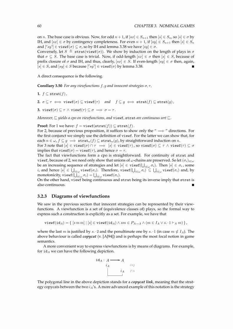
60 CHAPTER 3. NOMINAL GAMES
on n. The base case is obvious. Now, for odd n+ 1, if [sx] ∈ Sn+1 then [s] ∈ Sn, so [s] ∈ σ byIH, and [sx] ∈ σ by contingency completeness. For even n + 1, if [sy] ∈ Sn+1 then [s] ∈ Snand [psyq] ∈ viewf(σ) ⊆ σ, so by IH and lemma 3.38 we have [sy] ∈ σ.Conversely, let S , strat(viewf(σ)). We show by induction on the length of plays in σ
that σ ⊆ S. The base case is trivial. Now, if odd-length [sx] ∈ σ then [s] ∈ S, because of
prefix closure of σ and IH, and thus, clearly, [sx] ∈ S. If even-length [sy] ∈ σ then, again,[s] ∈ S, and [sy] ∈ S because [psyq] ∈ viewf(σ) by lemma 3.38. �
A direct consequence is the following.
Corollary 3.50 For any viewfunctions f, g and innocent strategies σ, τ ,
1. f ⊆ strat(f) ,
2. σ ⊆ τ ⇐⇒ viewf(σ) ⊆ viewf(τ) and f ⊆ g ⇐⇒ strat(f) ⊆ strat(g) ,
3. viewf(σ) ⊆ τ ∧ viewf(τ) ⊆ σ =⇒ σ = τ .
Moreover, ⊑ yields a cpo on viewfunctions, and viewf, strat are continuous wrt ⊑.
Proof: For 1 we have: f = viewf(strat(f)) ⊆ strat(f) .For 2, because of previous proposition, it suffices to show only the “ =⇒ ” directions. For
the first conjunct we simply use the definition of viewf. For the latter we can show that, for
each n ∈ ω, f ⊆ g =⇒ stratn(f) ⊆ stratn(g), by straightforward induction on n.For 3 note that [s] ∈ viewf(σ) ∩ τ =⇒ [s] ∈ viewf(τ) , so viewf(σ) ⊆ τ ∧ viewf(τ) ⊆ σ
implies that viewf(σ) = viewf(τ), and hence σ = τ .The fact that viewfunctions form a cpo is straightforward. For continuity of strat and
viewf, because of 2, we need only show that unions of ω-chains are preserved. So let (σi)i∈ωbe an increasing sequence of strategies and let [s] ∈ viewf(
⋃
i∈ω σi). Then [s] ∈ σi , somei, and hence [s] ∈
⋃
i∈ω viewf(σi). Therefore, viewf(⋃
i∈ω σi) ⊆⋃
i∈ω viewf(σi) and, by
monotonicity, viewf(⋃
i∈ω σi) =⋃
i∈ω viewf(σi).On the other hand, viewf being continuous and strat being its inverse imply that strat is
also continuous. �
3.2.3 Diagrams of viewfunctions
We saw in the previous section that innocent strategies can be represented by their view-functions. A viewfunction is a set of (equivalence classes of) plays, so the formal way to
express such a construction is explicitly as a set. For example, we have that
viewf(idA) = { [smm] | [s] ∈ viewf(idA) ∧ sm ∈ PA→A ∧ (m ∈ IA ∨ s.−1 ⊢A m) } ,
where the last m is justified by s.−2 and the penultimate one by s.−1 (in case m /∈ IA). The
above behaviour is called copycat (v. [AJ94]) and is perhaps the most focal notion in gamesemantics.
Amore convenient way to express viewfunctions is by means of diagrams. For example,
for idA we can have the following depiction.
AidA : // AiA OQ
iA PA
The polygonal line in the above depiction stands for a copycat link, meaning that the strat-
egy copycats between the two iA’s. Amore advanced example of this notation is the strategy
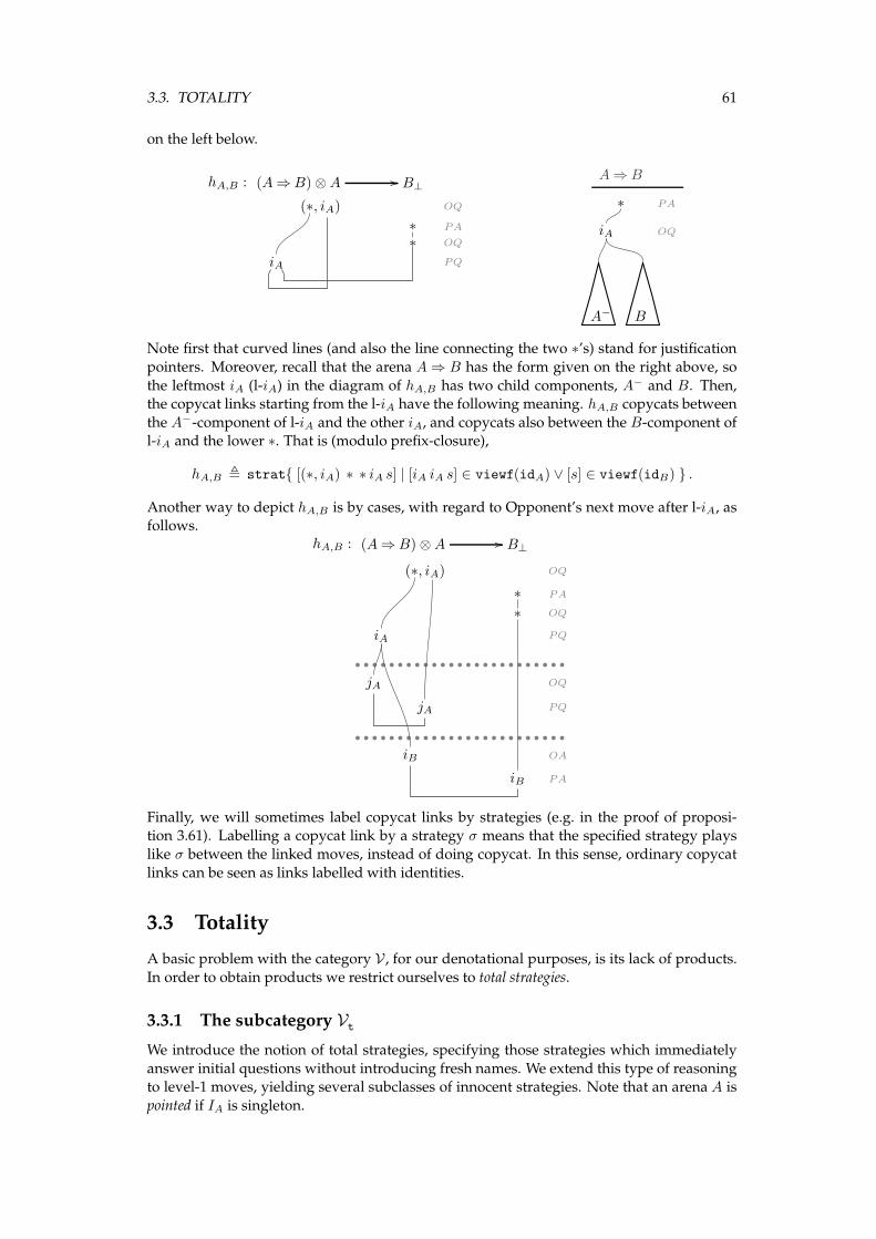
3.3. TOTALITY 61
on the left below.
(A⇒B) ⊗AhA,B : // B⊥
(∗, iA) OQ
∗ PA
∗ OQ
iA PQ
A⇒B
∗ PA
iA OQ
A− B
Note first that curved lines (and also the line connecting the two ∗’s) stand for justification
pointers. Moreover, recall that the arena A⇒ B has the form given on the right above, so
the leftmost iA (l-iA) in the diagram of hA,B has two child components, A− and B. Then,the copycat links starting from the l-iA have the following meaning. hA,B copycats between
the A−-component of l-iA and the other iA, and copycats also between the B-component ofl-iA and the lower ∗. That is (modulo prefix-closure),
hA,B , strat{ [(∗, iA) ∗ ∗ iA s] | [iA iA s] ∈ viewf(idA) ∨ [s] ∈ viewf(idB) } .
Another way to depict hA,B is by cases, with regard to Opponent’s next move after l-iA, asfollows.
(A⇒B) ⊗AhA,B : // B⊥
(∗, iA) OQ
∗ PA
∗ OQ
iA PQ
jA OQ
jA PQ
iB OA
iB PA
Finally, we will sometimes label copycat links by strategies (e.g. in the proof of proposi-tion 3.61). Labelling a copycat link by a strategy σ means that the specified strategy plays
like σ between the linked moves, instead of doing copycat. In this sense, ordinary copycat
links can be seen as links labelled with identities.
3.3 Totality
A basic problem with the category V , for our denotational purposes, is its lack of products.
In order to obtain products we restrict ourselves to total strategies.
3.3.1 The subcategory Vt
We introduce the notion of total strategies, specifying those strategies which immediately
answer initial questions without introducing fresh names. We extend this type of reasoningto level-1 moves, yielding several subclasses of innocent strategies. Note that an arena A is
pointed if IA is singleton.
62 CHAPTER 3. NOMINAL GAMES
Definition 3.51 (Vt, Vtt, Vt∗, Vtt∗) An innocent strategy σ : AB B is total if for any [iA] ∈σ there exists [iA iB] ∈ σ. A total strategy σ : AB B is:
• l4 if whenever [s] ∈ σ and s.−1 ∈ JA then | psq | = 4,
• t4 if for any [iA iB jB ] ∈ σ there exists [iA iB jB j~bA] ∈ σ,
• tl4 if it is both t4 and l4,
• ttotal if it is tl4 and for any [iA iB jB ] ∈ σ there exists [iA iB jB jA] ∈ σ.
A total strategy τ : C ⊗AB B is:
• l4* if whenever [s] ∈ τ and s.−1 ∈ JA then | psq | = 4,
• t4* if for any [(iC , iA)iB jB ] ∈ τ there exists [(iC , iA)iB jB j~bA] ∈ τ ,
• tl4* if it is both t4* and l4*,
• ttotal* if it is tl4* and for any [(iC , iA) iB jB ] ∈ σ there exists [(iC , iA) iB jB jA] ∈ σ.
We let Vt be the lluf subcategory of V of total strategies, and Vtt its lluf subcategory ofttotal strategies. Vt∗ and Vtt∗ are the full subcategories of Vt and Vtt respectively containing
pointed arenas. N
These subclasses of strategies will be demystified in the sequel. For now, note that l4 stands
for “linear in the 4th move”, and t4 for “total in the 4th move”.We now proceed to examine properties of Vt. Eventually, we will see that it contains fi-
nite products and distributive coproducts, that it contains some exponentials, and that liftingpromotes to a functor. Note that in the definitions to follow we will usually define strategies
by means of their viewfunctions modulo even-prefix closure.
3.3.2 Lifting and product
We first upgrade the lifting and tensor arena-constructions of definition 3.3 to functors.Eventually, tensor will give us products. In the following definition recall L from nota-
tion 3.7 and note that we write L(m) #m′ for L(m) ∩ S(m′) = ∅.
Definition 3.52 Let f : A → A′, g : B → B′ be arrows in Vt. Define the strategies f ⊗ g :
A⊗B → A′ ⊗B′ and f⊥ : A⊥ → A′⊥ as follows.
f ⊗ g , strat{ [(iA, iB) (iA′ , iB′) s] | ([iA iA′ s] ∈ viewf(f) ∧ [iB iB′ ] ∈ g ∧ L(iA iA′ s) # iB)
∨ ([iB iB′ s] ∈ viewf(g) ∧ [iA iA′ ] ∈ f ∧ L(iB iB′ s) # iA) }
f⊥ , strat{ [∗ ∗′ ∗′ ∗ s] | [s] ∈ viewf(f) } .N
Note that f⊥ is always ttotal. Let us we give an informal description of the above construc-tions:
• f⊥ : A⊥ → A′⊥ initially plays a sequence of asterisks [∗ ∗′ ∗′∗] and then continues
playing like f .
• f ⊗ g : A⊗B → A′⊗B′ answers initial moves [(iA, iB)] with f ’s answer to [iA] and g’sanswer to [iB]. Then, according to whether Opponent plays in JA′ or in JB′ , Player
plays like f or like g respectively.
We proceed to show that the above yield functors. The following lemma is straightforward
but arises quite often when we are dealing with definitions like that of f ⊗ g.
3.3. TOTALITY 63
Lemma 3.53 Let s1s and s2s be legal sequences of moves-with-names on a prearena A which bothsatisfy NC3, and s1, s2 be P-ending plays such that S(s2) ⊆ S(s1), L(s2s) # s1 and s1 appears in
ps1s′q, for any s′ ≤ s. Then, s1s is a play iff s2s is a play.
Proof: The claim is trivial if |s| = 0, so assume |s| > 0. For the “if”-part, we need to showNC1-2’. So let s′ ≤ s be P-ending sequence. If a ∈ nlist(s′.−1) and a # nlist(s′.−2) then
a # s2s′− and a ∈ L(s2s), so a # s1, s2s
′−, hence a # s1s′−. If a ∈ S(s′.−1) and a # ps1s′−q
then, since s1 appears in ps1s′q, a# ps2s′−q and hence a ∈ nlist(s′.−1).
For the “only if”-part, we again need to show NC1-2’. So let s′ ≤ s be P-ending sequence. If
a ∈ nlist(s′.−1) and a#nlist(s′.−2) then a# s1s′−, so a# s2s
′−. If a ∈ S(s′.−1) and a# ps2s′−qthen a ∈ L(s2s) so a# ps2s′−q, s1 , hence a# ps1s′−q and a ∈ nlist(s′.−1). �
Lemma 3.54 For f, f ′, g and g′ as above, the following are arrows in Vt.
f ⊗ g : A⊗B → A′ ⊗B′ , f⊥ : A⊥ → B⊥ .
Proof: For f ⊗ g, it suffices to show that φ is a viewfunction:
φ , { [(iA, iB) (iA′ , iB′) s] | ([iA iA′ s] ∈ viewf(f) ∧ [iB iB′ ] ∈ g ∧ L(iA iA′ s) # iB)
∨ ([iB iB′ s] ∈ viewf(g) ∧ [iA iA′ ] ∈ f ∧ L(iB iB′ s) # iA) } .
Elements in φ are plays: let [t] ∈ φ and suppose wlog that t = (iA, iB) (iA′ , iB′) s with
[iA iA′ s] ∈ viewf(f), [iB iB′ ] ∈ g and L(iA iA′ s) # iB. Then t is legal because iA iA′ s is.
Moreover, NC3 trivially holds and therefore, by previous lemma, t is a play.For even-prefix closure, let t = (iA, iB) (iA′ , iB′) sxy, [t] ∈ φ, and suppose, wlog, that
[iA iA′ sxy] ∈ viewf(f), [iB iB′ ] ∈ g and L(iA iA′ s) # iB. Then, [iA iA′ s] ∈ viewf(f) andthus [t−−] ∈ φ.
For single-valuedness, let [t1], [t2] ∈ φ and [t−1 ] = [t−2 ], say modulo π0 (i.e. t−1 = π0 [ t−2 ).If tκ = (iA(κ), iB(κ)) (iA′(κ), iB′(κ)) , for κ = 1, 2, then, by single-valuedness of viewf(f),[iA(1)] = [iA(2)] implies [iA(1) iA′(1)] = [iA(2) iA′(2)], and similarly [iB(1) iB′(1)] = [iB(2) iB′(2)].
Let’s say the former equality is modulo π1 and the latter is modulo π2. We now have iA(1) =
π0 [ iA(2) = π0 [π−11 [ iA(1) , ∴ iA′(1) = π0 [π−1
1 [ iA′(1) because S(iA′(1) ) ⊆ S(iA(1) ) ,
∴ iA(1) iA′(1) = π0 [ iA(2) iA′(2) , and similarly for the B-counterpart. Hence, t1 = π0 [ t2as required. If tκ = [(iA(κ), iB(κ)) (i′A′(κ), i
′B′(κ)) sκxκ], for κ = 1, 2, then suppose wlog that
[iB(κ) iB′(κ)] ∈ g and [iA(κ) iA′(κ) sκxκ] ∈ viewf(f), and L(iA(κ) iA′(κ) sκxκ) # iB(κ) . Then
[iA(1) iA′(1) s1] = [iA(2) iA′(2) s2], so [iA(1) iA′(1) s1x1] = [iA(2) iA′(2) s2x2]. Now using thestrong support lemma we get [t1] = [t2]. This completes the proof of “φ is a viewfunction”.
The case of f⊥ is similar (and simpler). �
Lemma 3.55 LetA,A′, B,B′ be arenas and iA,A′,B,B′ ∈ IA,A′,B,B′ respectively, and let sA and sBbe justified sequences of moves-with-names from IA ∪ IA′ and IB ∪ IB′ respectively. If f : AB A′
and g : BB B′ in Vt , then:
1. [(iA, iB) (iA′ , iB′) sA] ∈ f ⊗ g ⇐⇒ [iA iA′ sA] ∈ f ∧ [iB iB′ ] ∈ g ∧ L(iA iA′ sA) # iB ,
2. [(iA, iB) (iA′ , iB′) sB] ∈ f ⊗ g ⇐⇒ [iA iA′ ] ∈ f ∧ [iB iB′ sB] ∈ g ∧ L(iB iB′ sB) # iA ,
3. [∗ ∗ ∗ ∗ sA] ∈ f⊥ ⇐⇒ [sA] ∈ f .
Proof: For 1, let s = (iA, iB) (iA′ , iB′) sA, sf = iA iA′ sA and sg = iB iB′ . For “ =⇒ ”, wedo induction on |sA| ≥ 0 ; the base case is by definition. If |sA| is odd then, because of the
IH and contingency completeness of f , it suffices to show that sf is a play. But this followseasily from s and s−f being plays. If |sA| > 0 is even then, by IH and lemma 3.38, it suffices
to show that sf a play and that [psfq] ∈ f . Note that [psq] ∈ f ⊗ g implies psfq ∈ f and
L(psfq) # iB , and therefore, using also the IH, L(sf ) # iB . Moreover, sf is legal and satisfiesNC3 so we can use lemma 3.53.
For “⇐=”, we do again induction on |sA| ≥ 0 , and the base case is by definition. The case
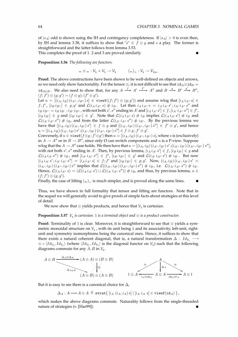
64 CHAPTER 3. NOMINAL GAMES
of |sA| odd is shown using the IH and contingency completeness. If |sA| > 0 is even then,by IH and lemma 3.38, it suffices to show that psq ∈ f ⊗ g and s a play. The former is
straightforward and the latter follows from lemma 3.53.This completes the proof of 1. 2 and 3 are proved similarly. �
Proposition 3.56 The following are functors.
⊗ : Vt × Vt → Vt ( )⊥ : Vt → Vtt∗
Proof: The above constructions have been shown to be well-defined on objects and arrows,
so we need only show functoriality. For the tensor⊗, it is not difficult to see that idA⊗idB =
idA⊗B . We also need to show that, for any AfPA A′ f ′PPA A′′ and B
gPA B′ g′PA B′′,(f ; f ′) ⊗ (g; g′) = (f ⊗ g); (f ′ ⊗ g′).
Let u = [(iA, iB) (iA′′ , iB′′) s] ∈ viewf((f ; f ′) ⊗ (g; g′)) and assume wlog that [iA iA′′ s] ∈f ; f ′ , [iB iB′′ ] ∈ g; g′ and L(iA iA′′ s) # iB . Let then iA iA′′ s = iA iA′ s′ ; iA′ iA′′ s′′ and
iB iB′′ = iB iB′ ; iB′ iB′′ , with not both s′, s′′ ending inA′ and [iA iA′ s′] ∈ f , [iA′ iA′′ s′′] ∈ f ′,
[iB iB′ ] ∈ g and [iB′ iB′′ ] ∈ g′. Note that L(iA iA′′ s) # iB implies L(iA iA′ s′) # iB andL(iA′ iA′′ s′′) # iB , and from the latter L(iA′ iA′′ s′′) # iB′ . By the previous lemma we
have that [(iA, iB) (iA′ , iB′) s′] ∈ f ⊗ g and [(iA′ , iB′) (iA′′ , iB′′) s′′] ∈ f ′ ⊗ g′, and henceu = [(iA, iB) (iA′ , iB′) s′ ;(iA′ , iB′) (iA′′ , iB′′) s′′] ∈ f ⊗ g ; f ′ ⊗ g′.
Conversely, if u ∈ viewf(f⊗g ; f ′⊗g′) then u = [(iA, iB) (iA′′ , iB′′) s], where s is (exclusively)
in A → A′′ or in B → B′′, since only O can switch components and u is a P-view. Supposewlog that theA→ A′′ case holds. We then have that u = [(iA, iB) (iA′ , iB′) s′ ;(iA′ , iB′) (iA′′ , iB′′) s′′],
with not both s′, s′′ ending in A′. Then, by previous lemma, [iA iA′ s′] ∈ f , [iB iB′ ] ∈ g andL(iA iA′ s′′) # iB , and [iA′ iA′′ s′′] ∈ f ′, [iB′ iB′′ ] ∈ g′ and L(iA′ iA′′ s′) # iB′ . But now
[iA iA′ s′ ; iA′ iA′′ s′′] = [iA iA′′ s] ∈ f ; f ′ and [iB iB′′ ] ∈ g; g′. Now, (iA, iB) (iA′ , iB′) s′ ≍(iA′ , iB′) (iA′′ , iB′′) s′′ implies that L((iA′ , iB′) (iA′′ , iB′′) s′′) # iB , i.e. L(iA′ iA′′ s′′) # iB .Hence, L(iA iA′′ s) = (L(iA iA′ s′) ∪ L(iA′ iA′′ s′′)) # iB , and thus, by previous lemma, u ∈(f ; f ′) ⊗ (g; g′).Finally, the case of lifting ( )⊥ is much simpler, and is proved along the same lines. �
Thus, we have shown in full formality that tensor and lifting are functors. Note that inthe sequel we will generally avoid to give proofs of simple facts about strategies at this level
of detail.
We now show that ⊗ yields products, and hence that Vt is cartesian.
Proposition 3.57 Vt is cartesian: 1 is a terminal object and ⊗ is a product constructor.
Proof: Terminality of 1 is clear. Moreover, it is straightforward to see that ⊗ yields a sym-metric monoidal structure on Vt , with its unit being 1 and its associativity, left-unit, right-
unit and symmetry isomorphisms being the canonical ones. Hence, it suffices to show that
there exists a natural coherent diagonal, that is, a natural transformation ∆ : IdVtB
⊗ ◦ 〈IdVt, IdVt
〉 (where 〈IdVt, IdVt
〉 is the diagonal functor on Vt) such that the following
diagrams commute for any A,B in Vt.
A⊗B
∆A⊗B **TTTTTTTTTTTTTTTTT
∆A⊗∆B // (A⊗A) ⊗ (B ⊗B)
(A⊗B) ⊗ (A⊗B)��∼=
A∼=
xxpppppppppppp
∆A
��
∼=
&&NNNNNNNNNNNN
1 ⊗A A⊗ A!A⊗idA
ooidA⊗!A
// A⊗ 1
But it is easy to see there is a canonical choice for ∆,
∆A : AB A⊗A , strat{ [iA (iA, iA) s] | [iA iA s] ∈ viewf(idA) } ,
which makes the above diagrams commute. Naturality follows from the single-threaded
nature of strategies (v. [Har99]). �
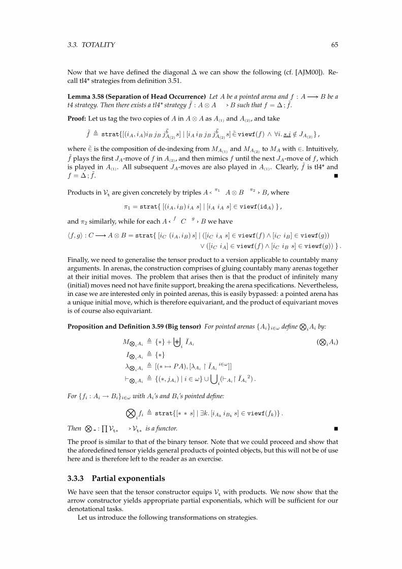
3.3. TOTALITY 65
Now that we have defined the diagonal ∆ we can show the following (cf. [AJM00]). Re-
call tl4* strategies from definition 3.51.
Lemma 3.58 (Separation of Head Occurrence) Let A be a pointed arena and f : AB B be at4 strategy. Then there exists a tl4* strategy f : A⊗AB B such that f = ∆ ; f .
Proof: Let us tag the two copies of A in A⊗A as A(1) and A(2), and take
f , strat{[(iA, iA)iB jB j~bA(2)
s] | [iA iB jB j~bA(2)
s] ∈ viewf(f) ∧ ∀i. s.i /∈ JA(2)} ,
where ∈ is the composition of de-indexing fromMA(1)andMA(2)
toMA with ∈. Intuitively,
f plays the first JA-move of f in A(2), and then mimics f until the next JA-move of f , which
is played in A(1). All subsequent JA-moves are also played in A(1). Clearly, f is tl4* and
f = ∆ ; f . �
Products in Vt are given concretely by triples Aπ1QPP A⊗B
π2PPA B, where
π1 = strat{ [(iA, iB) iA s] | [iA iA s] ∈ viewf(idA) } ,
and π2 similarly, while for each AfQP C gPA B we have
〈f, g〉 : CB A⊗B = strat{ [iC (iA, iB) s] | ([iC iA s] ∈ viewf(f) ∧ [iC iB] ∈ viewf(g))
∨ ([iC iA] ∈ viewf(f) ∧ [iC iB s] ∈ viewf(g)) } .
Finally, we need to generalise the tensor product to a version applicable to countably manyarguments. In arenas, the construction comprises of gluing countably many arenas together
at their initial moves. The problem that arises then is that the product of infinitely many
(initial) moves need not have finite support, breaking the arena specifications. Nevertheless,in case we are interested only in pointed arenas, this is easily bypassed: a pointed arena has
a unique initial move, which is therefore equivariant, and the product of equivariant moves
is of course also equivariant.
Proposition and Definition 3.59 (Big tensor) For pointed arenas {Ai}i∈ω define⊗
iAi by:
MN
iAi, {∗} +
⊎
iIAi
(⊗
iAi)
IN
iAi, {∗}
λN
iAi, [(∗ 7→ PA), [λAi
↾ IAi
i∈ω]]
⊢N
iAi, {(∗, jAi
) | i ∈ ω} ∪⋃
i(⊢Ai
↾ IAi
2) .
For {fi : Ai → Bi}i∈ω with Ai’s and Bi’s pointed define:
⊗
ifi , strat{[∗ ∗ s] | ∃k. [iAk
iBks] ∈ viewf(fk)} .
Then⊗
:∏
Vt∗ B Vt∗ is a functor. �
The proof is similar to that of the binary tensor. Note that we could proceed and show that
the aforedefined tensor yields general products of pointed objects, but this will not be of usehere and is therefore left to the reader as an exercise.
3.3.3 Partial exponentials
We have seen that the tensor constructor equips Vt with products. We now show that the
arrow constructor yields appropriate partial exponentials, which will be sufficient for ourdenotational tasks.
Let us introduce the following transformations on strategies.
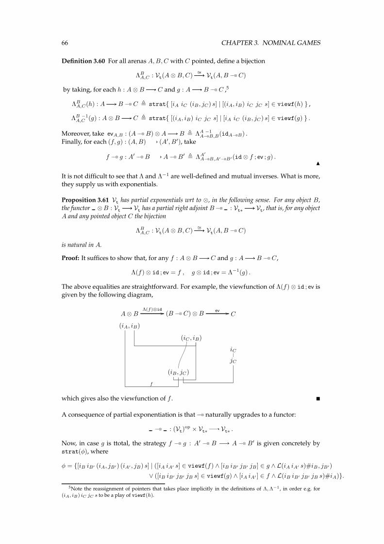
66 CHAPTER 3. NOMINAL GAMES
Definition 3.60 For all arenas A,B,C with C pointed, define a bijection
ΛBA,C : Vt(A⊗B,C)∼=PA Vt(A,B −−⊗ C)
by taking, for each h : A⊗BB C and g : AB B −−⊗ C ,5
ΛBA,C(h) : AB B −−⊗ C , strat{ [iA iC (iB, jC) s] | [(iA, iB) iC jC s] ∈ viewf(h) } ,
ΛB −1A,C (g) : A⊗BB C , strat{ [(iA, iB) iC jC s] | [iA iC (iB, jC) s] ∈ viewf(g) } .
Moreover, take evA,B : (A −−⊗ B) ⊗AB B , ΛA −1A−−⊗B,B(idA−−⊗B) .
Finally, for each (f, g) : (A,B) B (A′, B′), take
f −−⊗ g : A′−−⊗ BB A −−⊗ B′ , ΛA
′
A−−⊗B,A′−−⊗B′(id⊗ f ; ev ; g) .N
It is not difficult to see that Λ and Λ−1 are well-defined and mutual inverses. What is more,they supply us with exponentials.
Proposition 3.61 Vt has partial exponentials wrt to ⊗, in the following sense. For any object B,the functor ⊗B : Vt B Vt has a partial right adjoint B −−⊗ : Vt∗ B Vt, that is, for any object
A and any pointed object C the bijection
ΛBA,C : Vt(A⊗B,C)∼=PA Vt(A,B −−⊗ C)
is natural in A.
Proof: It suffices to show that, for any f : A⊗BB C and g : AB B −−⊗ C,
Λ(f) ⊗ id ; ev = f , g ⊗ id ; ev = Λ−1(g) .
The above equalities are straightforward. For example, the viewfunction of Λ(f) ⊗ id ; ev isgiven by the following diagram,
A⊗BΛ(f)⊗id // (B −−⊗ C) ⊗B
ev // C
(iA, iB)
(iC , iB)
iC
jC
(iB, jC)
f
which gives also the viewfunction of f . �
A consequence of partial exponentiation is that −−⊗ naturally upgrades to a functor:
−−⊗ : (Vt)op × Vt∗ B Vt∗ .
Now, in case g is ttotal, the strategy f −−⊗ g : A′−−⊗ B B A −−⊗ B′ is given concretely by
strat(φ), where
φ = {[iB iB′ (iA, jB′) (iA′ , jB) s] | ([iA iA′ s] ∈ viewf(f) ∧ [iB iB′ jB′ jB] ∈ g ∧ L(iA iA′ s)#iB , jB′)
∨ ([iB iB′ jB′ jB s] ∈ viewf(g) ∧ [iA iA′ ] ∈ f ∧ L(iB iB′ jB′ jB s)#iA)}.
5Note the reassignment of pointers that takes place implicitly in the definitions of Λ,Λ−1, in order e.g. for(iA, iB) iC jC s to be a play of viewf(h).
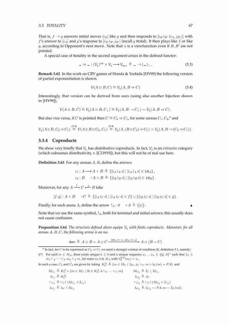
3.3. TOTALITY 67
That is, f −−⊗ g answers initial moves [iB] like g and then responds to [iB iB′ (iA, jB′)] withf ’s answer to [iA] and g’s response to [iB iB′ jB′ ] (recall g ttotal). It then plays like f or like
g, according to Opponent’s next move. Note that φ is a viewfunction even if B,B′ are notpointed.
A special case of ttotality in the second argument arises in the defined functor:
⇒ : (Vt)op × Vt B Vtt∗ , −−⊗ ( )⊥ . (3.3)
Remark 3.62 In the work on CBV games of Honda & Yoshida [HY99] the following versionof partial exponentiation is shown.
V(A⊗B,C) ∼= Vt(A,B⇒ C) (3.4)
Interestingly, that version can be derived from ours (using also another bijection shownin [HY99]),
V(A⊗B,C) ∼= Vt(A⊗B,C⊥) ∼= Vt(A,B −−⊗ C⊥) = Vt(A,B⇒ C) .
But also vice versa, if C is pointed then C ∼= C2 ⇒ C1, for some arenas C1, C2,6 and
Vt(A⊗B,C2⇒C1)(3.4)∼= V(A⊗B⊗C2, C1)
(3.4)∼= Vt(A, (B⊗C2)⇒C1) = Vt(A,B −−⊗(C2⇒C1)) .
3.3.4 Coproducts
We show very briefly that Vt has distributive coproducts. In fact, Vt is an extensive category(which subsumes distributivity, v. [CLW93]), but this will not be of real use here.
Definition 3.63 For any arenas A,B, define the arrows:
ι1 : AB A+ B , {[iA iA s] | [iA iA s] ∈ idA} ,
ι2 : BB A+B , {[iB iB s] | [iB iB s] ∈ idB} .
Moreover, for any AfPA C
gQP B take
[f, g] : A+BB C , {[iA iC s] | [iA iC s] ∈ f} ∪ {[iB iC s] | [iB iC s] ∈ g} .
Finally, for each arena A, define the arrow !A : 0B A , {[ǫ]} . N
Note that we use the same symbol, !A, both for terminal and initial arrows; this usually does
not cause confusion.
Proposition 3.64 The structure defined above equips Vt with finite coproducts. Moreover, for allarenas A,B,C, the following arrow is an iso.
dst , A⊗B +A⊗ C[idA ⊗ ι1, idA ⊗ ι2]PPPPPPPPPPPPPPA A⊗ (B + C)
6 In fact, for C to be expressed as C2 ⇒ C1 we need a stronger version of condition (f), definition 3.1, namely:
(f’) For each m ∈ MA, there exists unique k ≥ 0 and a unique sequence x1 . . . xn ∈ {Q, A}∗ such that IA ∋
m1 ⊢A · · · ⊢A mk ⊢A m , for some ml’s in MA with λQAC (ml) = xl .
In such a case, C1 and C2 are given by taking KAC , {m ∈ MC | ∃jC . jC ⊢C m ∧ λC(m) = PA} and
MC1, KA
C + {m ∈ MC | ∃k ∈ KAC . k ⊢C · · · ⊢C m} MC2
, IC \ MC1
IC1, KA
C IC2, JC
⊢C1, ⊢C↾ (MC1
× IC1) ⊢C2
, ⊢C↾ (MC2× IC2
)
λC1, λC ↾ MC1
λC2, [iC2
7→ PA, m 7→ λC(m)] .
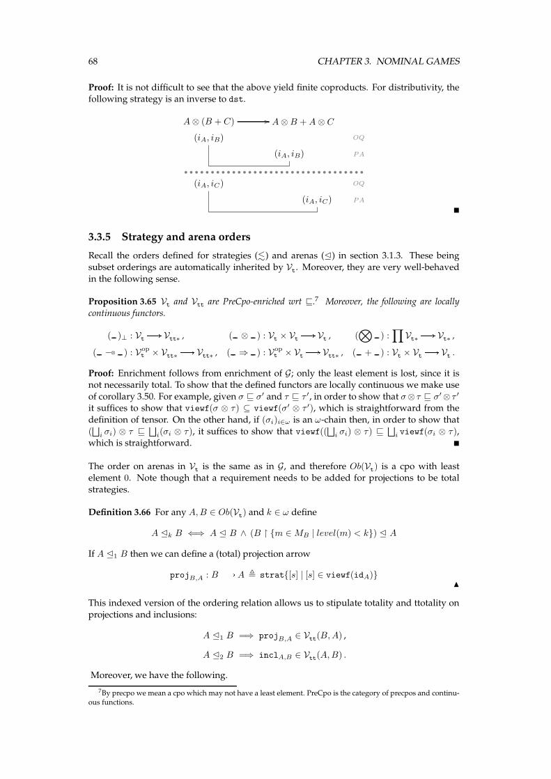
68 CHAPTER 3. NOMINAL GAMES
Proof: It is not difficult to see that the above yield finite coproducts. For distributivity, thefollowing strategy is an inverse to dst.
A⊗ (B + C) // A⊗B +A⊗ C
(iA, iB) OQ
(iA, iB) PA
(iA, iC) OQ
(iA, iC) PA
�
3.3.5 Strategy and arena orders
Recall the orders defined for strategies (.) and arenas (E) in section 3.1.3. These being
subset orderings are automatically inherited by Vt. Moreover, they are very well-behaved
in the following sense.
Proposition 3.65 Vt and Vtt are PreCpo-enriched wrt ⊑.7 Moreover, the following are locally
continuous functors.
( )⊥ : Vt B Vtt∗ , ( ⊗ ) : Vt × Vt B Vt , (⊗
) :∏
Vt∗ B Vt∗ ,
( −−⊗ ) : Vopt × Vtt∗ B Vtt∗ , ( ⇒ ) : Vop
t × Vt B Vtt∗ , ( + ) : Vt × Vt B Vt .
Proof: Enrichment follows from enrichment of G; only the least element is lost, since it isnot necessarily total. To show that the defined functors are locally continuous we make use
of corollary 3.50. For example, given σ ⊑ σ′ and τ ⊑ τ ′, in order to show that σ⊗ τ ⊑ σ′⊗ τ ′
it suffices to show that viewf(σ ⊗ τ) ⊆ viewf(σ′ ⊗ τ ′), which is straightforward from the
definition of tensor. On the other hand, if (σi)i∈ω is an ω-chain then, in order to show that
(⊔
i σi) ⊗ τ ⊑⊔
i(σi ⊗ τ), it suffices to show that viewf((⊔
i σi) ⊗ τ) ⊑⊔
i viewf(σi ⊗ τ),which is straightforward. �
The order on arenas in Vt is the same as in G, and therefore Ob(Vt) is a cpo with leastelement 0. Note though that a requirement needs to be added for projections to be total
strategies.
Definition 3.66 For any A,B ∈ Ob(Vt) and k ∈ ω define
A Ek B ⇐⇒ A E B ∧ (B ↾ {m ∈MB | level(m) < k}) E A
If A E1 B then we can define a (total) projection arrow
projB,A : BB A , strat{[s] | [s] ∈ viewf(idA)}N
This indexed version of the ordering relation allows us to stipulate totality and ttotality on
projections and inclusions:
A E1 B =⇒ projB,A ∈ Vtt(B,A) ,
A E2 B =⇒ inclA,B ∈ Vtt(A,B) .
Moreover, we have the following.
7By precpo we mean a cpo which may not have a least element. PreCpo is the category of precpos and continu-ous functions.
3.4. A MONAD, AND SOME COMONADS 69
Proposition 3.67 All of the functors of proposition 3.65 are continuous wrt E . Moreover,
A E A′ ∧B E B′ =⇒ inclA,A′⊗inclB,B′ = inclA⊗B,A′⊗B′
A E1 A′ ∧B E1 B
′ =⇒ projA′,A⊗projB′,B = projA′⊗B′,A⊗B
∀i ∈ ω.Ai E A′i =⇒
⊗
iinclAi,A′
i= inclN
iAi,N
iA′i
∀i ∈ ω.Ai E A′i =⇒
⊗
iprojA′
i,Ai= projN
iA′i,
N
iAi
A E1 A′ ∧B E B′ =⇒ projA′,A ⇒ inclB,B′ = inclA⇒B,A′⇒B′
A E A′ ∧B E1 B′ =⇒ inclA,A′ ⇒ projB′,B = projA′⇒B′,A⇒B
A E1 A′ ∧B E2 B
′ =⇒ projA′,A−−⊗ inclB,B′ = inclA−−⊗B,A′−−⊗B′
A E A′ ∧B E1 B′ =⇒ inclA,A′ −−⊗ projB′,B = projA′−−⊗B′,A−−⊗B
A E A′ ∧B E B′ =⇒ inclA,A′ + inclB,B′ = inclA+B,A′+B′
A E1 A′ ∧B E1 B
′ =⇒ projA′,A + projB′,B = projA′+B′,A+B
Proof: It is not difficult to show E-continuity. Now, all the above clauses are in effect spe-cial cases of functoriality statements, since the underlying sets of inclusions and projections
correspond to identity strategies. �
3.4 A monad, and some comonads
We now proceed to construct a monad and a family of comonads on Vt that will be of use
in later chapters. Specifically, we will upgrade lifting to a monad and introduce a family of
product comonads for initial state.
3.4.1 Lifting monad
It is a more-or-less standard result that the lifting functor induces a monad.
Definition 3.68 (Lifting monad) Define the natural transformations up, dn, st as follows.
upA : AB A⊥ = strat{ [iA ∗1 ∗2 iA s] | [iA iA s] ∈ viewf(idA) }
dnA : A⊥⊥ B A⊥ , strat{ [∗1 ∗′1 ∗
′2 ∗2 ∗3 ∗4 s] | [s] ∈ viewf(idA) }
stA,B : A⊗B⊥ B (A⊗B)⊥ , strat{ [(iA, ∗1) ∗′1 ∗
′2 ∗2 iB (iA, iB) s]
| [(iA, iB) (iA, iB) s] ∈ viewf(idA⊗B) }
(primed asterisks are used for arenas on the RHS, where necessary). N
Proposition 3.69 The quadruple (( )⊥, up, dn, st) is a strong monad on Vt. Moreover, it yields
monadic exponentials by taking (C⊥)B to be B⇒ C, for each B,C.
Proof: It is not difficult to see that (( )⊥, up, dn, st) is a strong monad. Moreover, for each
B,C we have that B⇒C = B −−⊗C⊥ is a ( )⊥-exponential, because of exponentiation prop-
erties of −−⊗. �
Although finding a canonical arrow from A to A⊥ is elementary (upA), finding a canoni-cal arrow in the inverse direction is not always possible. In some cases, e.g. A = Ai , there isno such arrow at all, let alone canonical. An exception occurs when A is pointed.
Definition 3.70 For any pointed arena A define:
puA : A⊥ B A , strat{ [∗ iA jA ∗ iA jA s] | [iA iA jA jA s] ∈ viewf(idA) } .N
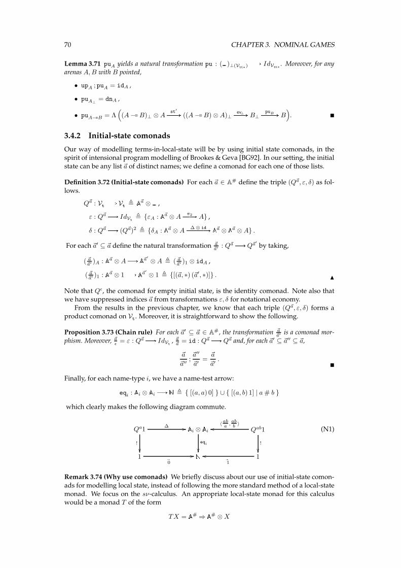
70 CHAPTER 3. NOMINAL GAMES
Lemma 3.71 puA yields a natural transformation pu : ( )⊥(Vtt∗) B IdVtt∗. Moreover, for any
arenas A,B with B pointed,
• upA ; puA = idA ,
• puA⊥= dnA ,
• puA−−⊗B = Λ(
(A −−⊗ B)⊥ ⊗Ast
′PPA ((A −−⊗ B) ⊗A)⊥ev⊥PPA B⊥
puBPPPA B)
. �
3.4.2 Initial-state comonads
Our way of modelling terms-in-local-state will be by using initial state comonads, in thespirit of intensional programmodelling of Brookes & Geva [BG92]. In our setting, the initial
state can be any list ~a of distinct names; we define a comonad for each one of those lists.
Definition 3.72 (Initial-state comonads) For each ~a ∈ A# define the triple (Q~a, ε, δ) as fol-
lows.
Q~a : Vt B Vt , A~a ⊗ ,
ε : Q~aB IdVt, {εA : A~a ⊗A
π2PPA A} ,
δ : Q~aB (Q~a)2 , {δA : A~a ⊗A∆ ⊗ idPPPPPA A~a ⊗ A~a ⊗A} .
For each ~a′ ⊆ ~a define the natural transformation ~a~a′ : Q~aB Q~a
′
by taking,
( ~a~a′ )A : A~a ⊗ AB A~a′ ⊗A , ( ~a~a′ )1 ⊗ idA ,
( ~a~a′ )1 : A~a ⊗ 1B A~a′ ⊗ 1 , {[(~a, ∗) (~a′, ∗)]} . N
Note that Qǫ, the comonad for empty initial state, is the identity comonad. Note also thatwe have suppressed indices ~a from transformations ε, δ for notational economy.
From the results in the previous chapter, we know that each triple (Q~a, ε, δ) forms aproduct comonad on Vt. Moreover, it is straightforward to show the following.
Proposition 3.73 (Chain rule) For each ~a′ ⊆ ~a ∈ A#, the transformation ~a~a′ is a comonad mor-
phism. Moreover, ~aǫ = ε : Q~aB IdVt, ~a~a = id : Q~aB Q~a and, for each ~a′ ⊆ ~a′′ ⊆ ~a,
~a
~a′′;~a′′
~a′=~a
~a′.
�
Finally, for each name-type i, we have a name-test arrow:
eqi : Ai ⊗ AiB N , { [(a, a) 0] } ∪ { [(a, b) 1] | a# b }
which clearly makes the following diagram commute.
Qa1∆ //
!
��
Ai ⊗ Aieqi
��
Qab1〈aba ,
abb 〉
oo
!
��1 b
0
// N 1b1
oo
(N1)
Remark 3.74 (Why use comonads) We briefly discuss about our use of initial-state comon-
ads for modelling local state, instead of following the more standard method of a local-state
monad. We focus on the sν-calculus. An appropriate local-state monad for this calculuswould be a monad T of the form
TX = A# ⇒ A# ⊗X
3.4. A MONAD, AND SOME COMONADS 71
and would entail that each typed term ~a ^ Γ_M : A be translated to a morphism JMK :
JΓK B A# ⇒ (A# ⊗ JAK), or, equivalently,
JMK : A# ⊗ JΓK B (A# ⊗ JAK)⊥ .
However, the generic treatment of initial state in the above description is inadequate for our
purposes. A# contains all possible initial states, and JMK would have to be specified for
each single one of these— even for irrelevant ones.What seemsmore fitting to our nominal framework is a translation to specific initial states,
up to permutation, which concretely means
JMK : A~a ⊗ JΓK B (A# ⊗ JAK)⊥
in our running example. But since in nominal games all information pertaining fresh names
is embedded in moves (cf. [AGM+04, Ong02]), the appearance of A# in the RHS above isredundant. Hence, the desired interpretation boils down to
JMK : A~a ⊗ JΓK B JAK⊥
which is precisely the (underlying) interpretation pursued in the next chapters.
3.4.3 Fresh-name constructors
Combining the monad and comonads of the previous sections we can obtain a monadic-
comonadic setting (Vt, ( )⊥, Q), where by Q we denote the family (Q~a)~a∈A# . This setting,which in fact yields a sound model of the sν-calculus, will be used as the basis of our se-
mantics of nominal computation in the sequel. As discussed in remark 3.74, nominal com-
putation of type A, in name-environment ~a and variable-environment Γ, will be translatedin the set of strategies
{ σ : Q~aJΓK B JAK⊥ } .
The lifting functor, representing the monadic part of our semantical setting, will therefore
incorporate the computational effect of fresh-name creation.We describe in this section the game-semantical expression of fresh-name creation. Fresh
names are created by means of natural transformations which transform a comonadQ~a, say,
to a monad-comonad composite (Q~aa )⊥.
Definition 3.75 Consider the setting (Vt, ( )⊥, Q). We define, for each ~aa ∈ A#, naturaltransformations
new~aa : Q~aB (Q~aa )⊥
by:
new~aaA , A~a ⊗Anew
~aa1 ⊗ idAPPPPPPPPPA (A~aa)⊥ ⊗A
st′PPA (A~aa ⊗A)⊥ ,
new~aa1 : A~a ⊗ 1 B (A~aa ⊗ 1)⊥ , strat{[(~a, ∗) ∗ ∗ (~aa, ∗)a]} .N
We will usually omit superscripts in new, for economy. That new is a natural transformation
is straightforward: for any f : AB B we can form the following commutative diagram.A~a ⊗A
id⊗f
��
new1⊗id // (A~aa)⊥ ⊗ A
id⊗f
��
st′
// (A~aa ⊗A)⊥
(id⊗f)⊥
��A~a ⊗Bnew1⊗id
// (A~aa)⊥ ⊗Bst
′// (A~aa ⊗B)⊥
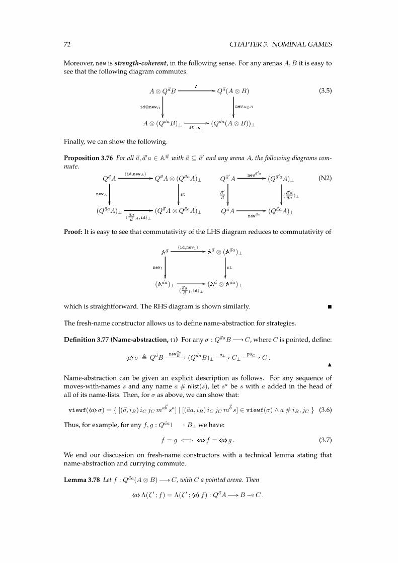
72 CHAPTER 3. NOMINAL GAMES
Moreover, new is strength-coherent, in the following sense. For any arenas A,B it is easy tosee that the following diagram commutes.
A⊗Q~aB
id⊗newB
��
z // Q~a(A⊗B)
newA⊗B
��A⊗ (Q~aaB)⊥
st ; z⊥ // (Q~aa(A⊗B))⊥
(3.5)
Finally, we can show the following.
Proposition 3.76 For all ~a,~a′a ∈ A# with ~a ⊆ ~a′ and any arena A, the following diagrams com-
mute.
Q~aA
newA
��
〈id,newA〉 // Q~aA⊗ (Q~aaA)⊥
st
��(Q~aaA)⊥
〈~aa~a A,id〉⊥
// (Q~aA⊗Q~aaA)⊥
Q~a′
Anew
~a′a//
~a′
~a
��
(Q~a′aA)⊥
(~a′a~aa )⊥
��Q~aA
new~aa
// (Q~aaA)⊥
(N2)
Proof: It is easy to see that commutativity of the LHS diagram reduces to commutativity ofA~anew1
��
〈id,new1〉 // A~a ⊗ (A~aa)⊥st
��(A~aa)⊥
〈~aa~a 1,id〉⊥
// (A~a ⊗ A~aa)⊥which is straightforward. The RHS diagram is shown similarly. �
The fresh-name constructor allows us to define name-abstraction for strategies.
Definition 3.77 (Name-abstraction, \ ℄) For any σ : Q~aaBB C, whereC is pointed, define:\a℄σ , Q~aBnew
~aaBPPPPA (Q~aaB)⊥
σ⊥PPA C⊥puCPPPA C .
N
Name-abstraction can be given an explicit description as follows. For any sequence ofmoves-with-names s and any name a # nlist(s), let sa be s with a added in the head of
all of its name-lists. Then, for σ as above, we can show that:
viewf(\a℄σ) = { [(~a, iB) iC jC ma~b sa] | [(~aa, iB) iC jC m
~b s] ∈ viewf(σ) ∧ a# iB, jC } (3.6)
Thus, for example, for any f, g : Q~aa1B B⊥ we have:
f = g ⇐⇒ \a℄ f = \a℄ g . (3.7)
We end our discussion on fresh-name constructors with a technical lemma stating that
name-abstraction and currying commute.
Lemma 3.78 Let f : Q~aa(A⊗B) B C, with C a pointed arena. Then\a℄Λ(ζ ′ ; f) = Λ(ζ ′ ; \a℄ f) : Q~aAB B −−⊗ C .
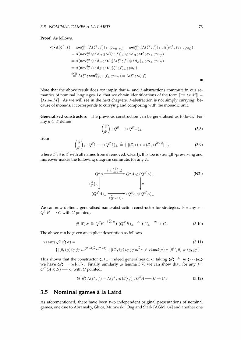
3.5. NOMINAL GAMES A LA LAIRD 73
Proof: As follows.\a℄Λ(ζ ′ ; f) = new~aaA ;(Λ(ζ ′ ; f))⊥ ; puB−−⊗C = new~aaA ;(Λ(ζ ′ ; f))⊥ ; Λ(st′ ; ev⊥ ; puC)
= Λ(new~aaA ⊗ idB ;(Λ(ζ ′ ; f))⊥ ⊗ idB ; st′ ; ev⊥ ; puC)
= Λ(new~aaA ⊗ idB ; st′ ;(Λ(ζ ′ ; f) ⊗ idB)⊥ ; ev⊥ ; puC)
= Λ(new~aaA ⊗ idB ; st′ ;(ζ ′ ; f)⊥ ; puC)
(N2)= Λ(ζ ′ ; new~aaA⊗B ; f⊥ ; puC) = Λ(ζ ′ ; \a℄ f)
�
Note that the above result does not imply that ν- and λ-abstractions commute in our se-mantics of nominal languages, i.e. that we obtain identifications of the form Jνa.λx.MK =
Jλx.νa.MK. As we will see in the next chapters, λ-abstraction is not simply currying: be-
cause of monads, it corresponds to currying and composing with the monadic unit.
Generalised constructors The previous construction can be generalised as follows. Forany ~a ⊆ ~a′ define
(~a
~a′
)
: Q~aB (Q~a′
)⊥ (3.8)
from (~a
~a′
)
1 : Q~a1B (Q~a′
1)⊥ , { [(~a, ∗) ∗ ∗ (~a′, ∗)~a′r~a] } , (3.9)
where ~a′ \~a is ~a′ with all names from ~a removed. Clearly, this too is strength-preserving and
moreover makes the following diagram commute, for any A.
Q~aA
(~a~a′
)
A
��
〈id,(~a~a′
)
A〉// Q~aA⊗ (Q~a
′
A)⊥
st
��(Q~a
′
A)⊥〈~a′
~a A,id〉⊥
// (Q~aA⊗Q~a′
A)⊥
(N2’)
We can now define a generalised name-abstraction constructor for strategies. For any σ :
Q~a′
BB C with C pointed,\~a^~a′℄σ , Q~aB
` ~a~a′
´
BPPPPA (Q~a′
B)⊥σ⊥PPA C⊥
puCPPPA C . (3.10)
The above can be given an explicit description as follows.
viewf( \~a^~a′℄σ) = (3.11)
{ [(~a, iB) iC jC m(~a′\~a)~b s(~a
′\~a)] | [(~a′, iB) iC jC m~b s] ∈ viewf(σ) ∧ (~a′ \ ~a) # iB, jC }
This shows that the constructor \ ^ ℄ indeed generalises \ ℄ : taking \~a′℄ , \a1℄ · · · \an℄we have \~a′℄ = \~a^~a~a′℄ . Finally, similarly to lemma 3.78 we can show that, for any f :
Q~a′
(A⊗B) B C with C pointed,\~a^~a′℄Λ(ζ ′ ; f) = Λ(ζ ′ ; \~a^~a′℄ f) : Q~aAB B −−⊗ C . (3.12)
3.5 Nominal games a la Laird
As aforementioned, there have been two independent original presentations of nominal
games, one due to Abramsky, Ghica, Murawski, Ong and Stark [AGM+04] and another one
74 CHAPTER 3. NOMINAL GAMES
due to Laird [Lai04, Lai08]. Although Laird’s constructions are not explicitly based on nom-inal sets (natural numbers are used instead of atoms), they constitute nominal constructions
nonetheless. In this section we highlight the main differences between our nominal games,which follow [AGM+04], and those of [Lai04, Lai08].
Laird’s presentation concerns the ν-calculus with pointers, i.e. with references to names.
The main difference in his presentation is in the treatment of name-introduction. In particu-lar, a name does not appear in a play at the point of evaluation of its ν-constructor, but rather
at the point of its first use; let us refer to this condition as name-frugality (cf. [MT09]). An im-mediate result is that strategies are no longer innocent, as otherwise e.g. νa.λx.a and λx.νa.a
would have the same denotation.8 More importantly, name-frugality implies that strategies
capture the examined nominal language more accurately: Opponent is not expected to guessnames he is not supposed to know and thus, for example, the denotations of νa.skip and
skip are identical. In our setting, Player is not frugal with his names and therefore the twoterms above are identified only at the extensional level (i.e. after quotienting).9
The major difference between [Lai04] and [Lai08] lies in the modelling of (ground-type,
name-storing) store. In [Lai04] the store is modelled by attaching to strategies a global, top-level (non-monadic), store-arena. Then, a good-store-discipline is imposed on strategies via
extra conditions on strategy composition which enforce that hidden store-moves follow thestandard read/write pattern. As a result (and in contrast to our model), the model relies
heavily on quotienting by the intrinsic preorder in order for the store to work properly.
The added accuracy obtained by using frugality conditions is fully exploited in [Lai08],where a carefully formulated setting of moves-with-store10 allows for an explicit character-
isation result, that is, a semantic characterisation of operational equality at the intensionallevel. The contribution of using moves-with-store in that result is that thus the seman-
tics is relieved from the (too revealing) internal workings of store: for example, terms like
(a := b) ;λx. ! a ; 0 and (a := b) ;λx.0 are equated semantically at the intensional level, incontrast to what happens in our model.11 Note, though, that in a setting with higher-order
store such that of νρ, moves-with-store would not be as simple since stores would need to
store higher-order values, that is, strategies.Laird’s approach is therefore advantageous in its use of name-frugality conditions, which
allow for more accurate models. At the same time, though, frugality conditions are an ex-tra burden in constructing a model: apart from the fact that they need to be dynamically
preserved in play-composition by garbage collection, they presuppose an appropriately de-
fined notion of name-use. In [Lai04, Lai08], a name is considered as used in a play if it isaccessible through the store (in a reflexive transitive manner) from a name that has been ex-
plicitly played. This definition, however, does not directly apply to languages with differentnominal effects (e.g. higher-order store). Moreover, frugality alone is not enough for lan-
guages like ReducedML [Sta94] or the ν-calculus: a namemay have been used in a play but
may still be inaccessible to some participant (e.g. if it is outside his view [MT09]). On theother hand, our approach is advantageous in its simplicity and its applicability on a wide
rage of nominal effects, but suffers from the accuracy issues discussed above.
8Non-innocence can be seen as beneficial in terms of simplicity of the model, since strategies then have onecondition less. On the other hand, though, innocent strategies are specified by means of their viewfunctions,which makes their presentation simpler. Moreover, non-innocence diminishes the power of definability results, asfinitary behaviours are less expressive in the absence of innocence.
9Note here, though, that the semantics being too explicit about the created names can prove beneficial: herewe are able to give a particularly concise proof adequacy for νρ (see section 4.3.4 and compare e.g. with respectiveproof in [AHM98]) by exploiting precisely this extra information!
10Inter alia, frugality of names implies that sequences of moves-with-store have strong support even if stores arerepresented by sets!
11In our model they correspond to the strategies (see also section 4.3):
σ1 , {[(a, b) ∗ ⊛(∗, ⊛)(n, ⊛) a c 0]} , σ2 , {[(a, b) ∗ ⊛(∗, ⊛)(n, ⊛) 0]} .
Thus, the inner-workings of the store revealed by σ1 (i.e. the moves a c) differentiate it from σ2. In fact, in ourattempts to obtain an explicit characterisation result from our model, we found store-related inaccuracies to be themost stubborn ones.

Chapter 4
Nominal References
In this chapter we construct in nominal games a fully abstract semantics for a languagewith nominal general references called the νρ-calculus. General references are references
which can store not only values of ground type (integers, booleans, etc.) but also of higher-
order type (procedures, higher-order functions) or references themselves. They constitutea very powerful and useful programming construct, allowing for the encoding of a wide
range of computational effects and programming paradigms (e.g. object-oriented program-ming [AHM98, section 2.3] or aspect-oriented programming [SO07]). The denotational
modelling of higher-order references is quite demanding since, on top of phenomena of dy-
namic update and interference, one has to cope with the inherent cyclicity of higher-orderstorage.
The νρ-calculus is a functional language with dynamically allocated general references,
reference-equality tests and “good variables”, which faithfully reflects the practice of realprogramming languages such as ML [MTM97]. In particular, it extends the sν-calculus by
using names for general references. In terms of the What’s new? motto (cf. [PS93]), namescan be
created with local scope, updated and dereferenced, tested for equality and passed around
via function application, but that is all.
The fully abstract model of νρ is the first such for a language with general references andgood variables.
Fully abstract models for general references were given via game semantics in [AHM98]and via abstract categorical semantics (and games) in [Lai02]. Neither approach used names.
The model of [AHM98] is based on the idea of relaxing strategy conditions in order to model
computational effects. In particular, it models references as variables of a read/write prod-uct type and it uses strategies which violate visibility in order to use values assigned to ref-
erences previously in a play. The synchronisation of references is managed by cell strategieswhich model fresh-reference creation. Because references are modelled by products, and
in order to produce a fully abstract semantics, the examined language needs to include bad
variables, which in turn yield unwanted behaviours affecting severely the expressivity of thelanguage, and prohibit the use of equality tests for references.1 On the other hand, the ap-
proach in [Lai02] bypasses the bad-variables problem by not including types for references(variables and references of the same type coincide). This contributes new intuitions on se-
quential categorical behaviour (sequoidal category), but we think that is somehow distanced
from the common notion of reference in functional programming.The full-abstraction problem has also been tackled via trace semantics in [Lai07]. The
language examined is a version of that in [AHM98] without bad variables. The latter are not
needed since the modelling of references is achieved by names pointing to a store (which
1By “bad variables” we mean read/write constructs of reference type which are not references. They are nec-essary for obtaining full-abstraction in [AHM98] since read/write-product semantical objects may not necessarilydenote references.
75
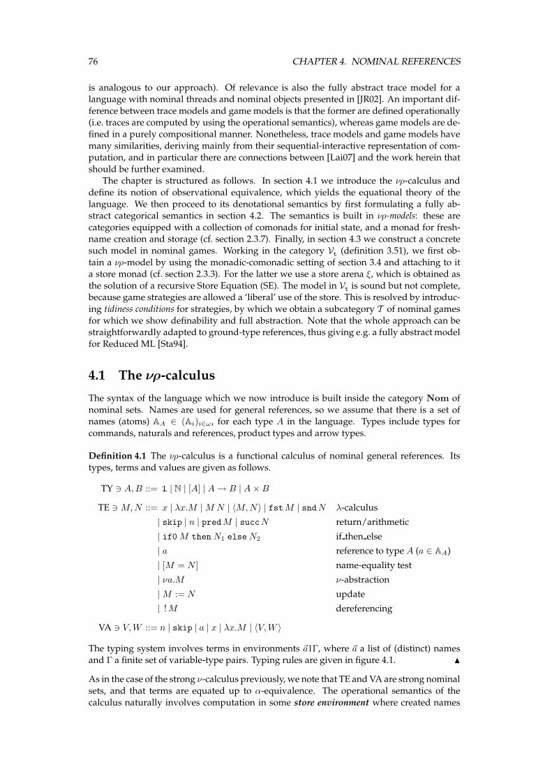
76 CHAPTER 4. NOMINAL REFERENCES
is analogous to our approach). Of relevance is also the fully abstract trace model for alanguage with nominal threads and nominal objects presented in [JR02]. An important dif-
ference between trace models and game models is that the former are defined operationally(i.e. traces are computed by using the operational semantics), whereas game models are de-
fined in a purely compositional manner. Nonetheless, trace models and game models have
many similarities, deriving mainly from their sequential-interactive representation of com-putation, and in particular there are connections between [Lai07] and the work herein that
should be further examined.The chapter is structured as follows. In section 4.1 we introduce the νρ-calculus and
define its notion of observational equivalence, which yields the equational theory of the
language. We then proceed to its denotational semantics by first formulating a fully ab-stract categorical semantics in section 4.2. The semantics is built in νρ-models: these are
categories equipped with a collection of comonads for initial state, and a monad for fresh-name creation and storage (cf. section 2.3.7). Finally, in section 4.3 we construct a concrete
such model in nominal games. Working in the category Vt (definition 3.51), we first ob-
tain a νρ-model by using the monadic-comonadic setting of section 3.4 and attaching to ita store monad (cf. section 2.3.3). For the latter we use a store arena ξ, which is obtained as
the solution of a recursive Store Equation (SE). The model in Vt is sound but not complete,because game strategies are allowed a ‘liberal’ use of the store. This is resolved by introduc-
ing tidiness conditions for strategies, by which we obtain a subcategory T of nominal games
for which we show definability and full abstraction. Note that the whole approach can bestraightforwardly adapted to ground-type references, thus giving e.g. a fully abstract model
for Reduced ML [Sta94].
4.1 The νρ-calculus
The syntax of the language which we now introduce is built inside the category Nom of
nominal sets. Names are used for general references, so we assume that there is a set ofnames (atoms) AA ∈ (Ai)i∈ω, for each type A in the language. Types include types for
commands, naturals and references, product types and arrow types.
Definition 4.1 The νρ-calculus is a functional calculus of nominal general references. Its
types, terms and values are given as follows.
TY ∋ A,B ::= 1 | N | [A] | A→ B | A×B
TE ∋M,N ::= x | λx.M |M N | 〈M,N〉 | fstM | sndN λ-calculus
| skip | n | predM | succN return/arithmetic
| if0M thenN1 elseN2 if then else
| a reference to type A (a ∈ AA)
| [M = N ] name-equality test
| νa.M ν-abstraction
|M := N update
| !M dereferencing
VA ∋ V,W ::= n | skip | a | x | λx.M | 〈V,W 〉
The typing system involves terms in environments ~a^Γ, where ~a a list of (distinct) namesand Γ a finite set of variable-type pairs. Typing rules are given in figure 4.1. N
As in the case of the strong ν-calculus previously, we note that TE and VA are strong nominal
sets, and that terms are equated up to α-equivalence. The operational semantics of the
calculus naturally involves computation in some store environment where created names

4.1. THE νρ-CALCULUS 77
~a ^ Γ_ n : N ~a ^ Γ, x :A_ x : A ~a ^ Γ_ skip : 1~a ^ Γ_M : A×B
~a ^ Γ_ fstM : A
~a ^ Γ_M : A×B
~a ^ Γ_ sndM : B
~a ^ Γ_M : A ~a ^ Γ_N : B
~a ^ Γ_ 〈M,N〉 : A×B
~a ^ Γ_M : N
~a ^ Γ_ predM : N
~a ^ Γ_M : N
~a ^ Γ_ succM : N
~a ^ Γ_M : N ~a ^ Γ_N1, N2 : A
~a ^ Γ_ if0M thenN1 elseN2 : A
~a ^ Γ, x :A_M : B
~a ^ Γ_ λx.M : A→ B
~a ^ Γ_M : A→ B ~a ^ Γ_N : A
~a ^ Γ_M N : B
a∈ AA
∧a∈~a~a ^ Γ_ a : [A]
~aa ^ Γ_M : B
~a ^ Γ_ νa.M : B
~a ^ Γ_M : [A] ~a ^ Γ_N : [A]
~a ^ Γ_ [M = N ] : N
~a ^ Γ_M : [A]
~a ^ Γ_ !M : A
~a ^ Γ_M : [A] ~a ^ Γ_N : A
~a ^ Γ_M := N : 1Figure 4.1: The νρ-calculus: typing rules.
have their values stored. Formally, we define store environments S to be lists of the form:
S ::= ǫ | a, S | a :: V, S . (4.1)
Observe that the store may include names that have been created but remain as yet unas-signed a value. For each store environment S we define its domain to be the name-list given
by:
dom(ǫ) , ǫ , dom(a, S) , a, dom(S) , dom(a :: V, S) , a, dom(S) . (4.2)
We only consider environments whose domains are lists of distinct names. Wewrite S `Γ,A
M , or simply S `M , only if dom(S) ^ Γ_M : A is valid (i.e. derivable).
Definition 4.2 The operational semantics is given in terms of a small-step reduction rela-tion, the rules of which are given in figure 4.2. Evaluation contexts E are of the forms:
(λx.N) , N , fst , snd , 〈 , N〉 , 〈V, 〉 , if0 thenN1 elseN2 ,
pred , succ , [ = N ] , [a = ] , ! , := N , a := .N
We can see that νρ is not strongly normalising with the following example. Recall the stan-
dard CBV encoding of sequencing:
M ;N , (λz.N)M (4.3)
with z /∈ fv(N).
Example 4.3 For each type A, take
stopA , νb.(b := λx.(! b)skip) ;(! b)skip
with b ∈ A1→A. We can see that stopA diverges, since:` stopA −→→ b :: λx.(! b)skip` (! b)skip
−−→ b :: λx.(! b)skip` (λx.(! b)skip)skip
−−→ b :: λx.(! b)skip` (! b)skip .
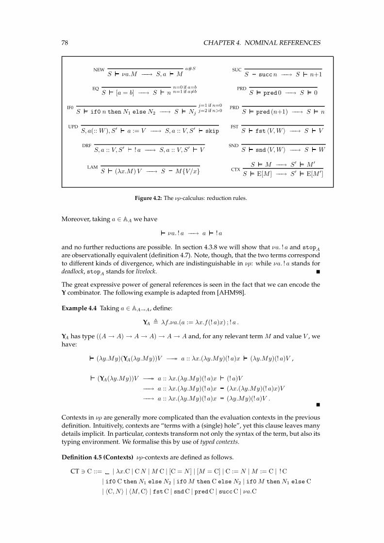
78 CHAPTER 4. NOMINAL REFERENCES
NEW a#S
S ` νa.M −−→ S, a`MSUC
S ` succn −−→ S ` n+1
EQ n=0 if a=bn=1 if a6=bS ` [a = b] −−→ S ` n
PRDS ` pred0 −−→ S ` 0
IF0j=1 if n=0j=2 if n>0S ` if0 n thenN1 elseN2 −−→ S ` Nj
PRDS ` pred (n+1) −−→ S ` n
UPDS, a(:: W ), S′ ` a := V −−→ S, a :: V, S′ ` skip
FSTS ` fst 〈V,W 〉 −−→ S ` V
DRFS, a :: V, S′ ` ! a −−→ S, a :: V, S′ ` V
SNDS ` snd 〈V,W 〉 −−→ S `W
LAMS ` (λx.M)V −−→ S `M{V/x} CTX
S `M −−→ S′ `M ′
S ` E[M ] −−→ S′ ` E[M ′]
Figure 4.2: The νρ-calculus: reduction rules.
Moreover, taking a ∈ AA we have ` νa. ! a −−→ a` !a
and no further reductions are possible. In section 4.3.8 we will show that νa. ! a and stopAare observationally equivalent (definition 4.7). Note, though, that the two terms correspond
to different kinds of divergence, which are indistinguishable in νρ: while νa. ! a stands fordeadlock, stopA stands for livelock. �
The great expressive power of general references is seen in the fact that we can encode theY combinator. The following example is adapted from [AHM98].
Example 4.4 Taking a ∈ AA→A, define:
YA , λf.νa.(a := λx.f(! a)x) ; ! a .
YA has type ((A → A) → A → A) → A → A and, for any relevant termM and value V , we
have: ` (λy.My)(YA(λy.My))V −→→ a :: λx.(λy.My)(! a)x` (λy.My)(! a)V ,` (YA(λy.My))V −→→ a :: λx.(λy.My)(! a)x` (! a)V
−−→ a :: λx.(λy.My)(! a)x` (λx.(λy.My)(! a)x)V
−−→ a :: λx.(λy.My)(! a)x` (λy.My)(! a)V .�
Contexts in νρ are generally more complicated than the evaluation contexts in the previous
definition. Intuitively, contexts are “terms with a (single) hole”, yet this clause leaves manydetails implicit. In particular, contexts transform not only the syntax of the term, but also its
typing environment. We formalise this by use of typed contexts.
Definition 4.5 (Contexts) νρ-contexts are defined as follows.
CT ∋ C ::= | λx.C | CN |M C | [C = N ] | [M = C] | C := N |M := C | ! C
| if0 C thenN1 elseN2 | if0M then C else N2 | if0M thenN1 else C
| 〈C, N〉 | 〈M,C〉 | fstC | sndC | predC | succC | νa.C
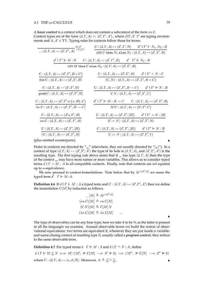
4.1. THE νρ-CALCULUS 79
A basic context is a context which does not contain a subcontext of the form νa.C.Context types are of the form (~a,Γ, A) 7→ (~a′,Γ′, A′) , where ~a^Γ,~a′^Γ′ are typing environ-
ments and A,A′ ∈ TY. Typing rules for contexts follow those for terms:
~a⊆~a′
∧Γ⊆Γ′ : (~a,Γ, A) 7→ (~a′,Γ′, A)
C : (~a,Γ, A) 7→ (~a′,Γ′,N) ~a′ ^ Γ′_N1, N2 : B
if0 C thenN1 elseN2 : (~a,Γ, A) 7→ (~a′,Γ′, B)
~a′ ^ Γ′_M : N C : (~a,Γ, A) 7→ (~a′,Γ′, B) ~a′ ^ Γ′_N2 : B
if0M then C elseN2 : (~a,Γ, A) 7→ (~a′,Γ′, B)
C : (~a,Γ, A) 7→ (~a′,Γ′, B × C)
fstC : (~a,Γ, A) 7→ (~a′,Γ′, B)
C : (~a,Γ, A) 7→ (~a′,Γ′, B) ~a′ ^ Γ′_N : C
〈C, N〉 : (~a,Γ, A) 7→ (~a′,Γ′, B × C)
C : (~a,Γ, A) 7→ (~a′,Γ′,N)
predC : (~a,Γ, A) 7→ (~a′,Γ′,N)
C : (~a,Γ, A) 7→ (~a′,Γ′, B → C) ~a′ ^ Γ′_N : B
CN : (~a,Γ, A) 7→ (~a′,Γ′, C)
C : (~a,Γ, A) 7→ (~a′,Γ′ ⊎ {x :B}, C)
λx.C : (~a,Γ, A) 7→ (~a′,Γ′, B → C)
~a′ ^ Γ′_M : B → C C : (~a,Γ, A) 7→ (~a′,Γ′, B)
M C : (~a,Γ, A) 7→ (~a′,Γ′, C)
C : (~a,Γ, A) 7→ (~a′a,Γ′, B)
νa.C : (~a,Γ, A) 7→ (~a′,Γ′, B)
C : (~a,Γ, A) 7→ (~a′,Γ′, [B]) ~a′ ^ Γ′_N : [B]
[C = N ] : (~a,Γ, A) 7→ (~a′,Γ′,N)
C : (~a,Γ, A) 7→ (~a′,Γ′, [B])
! C : (~a,Γ, A) 7→ (~a′,Γ′, B)
C : (~a,Γ, A) 7→ (~a′,Γ′, [B]) ~a′ ^ Γ′_N : B
C := N : (~a,Γ, A) 7→ (~a′,Γ′, 1)(plus omitted counterparts). N
Holes in contexts are denoted by “ ” (elsewhere, they are usually denoted by “[ ]”). In acontext of type (~a,Γ, A) 7→ (~a′,Γ′, A′) the type of its hole is (~a,Γ, A), and (~a′,Γ′, A′) is the
resulting type. The first typing rule above states that if has type (~a,Γ, A) then the typeof the context may have more names or more variables. This allows us to consider typed
terms ~a ^ Γ_M : A in all compatible contexts. Finally, note that contexts are not equated
up to α-equivalence.We now proceed to context-instantiations. Note below that by M+(~a′\~a) we mean the
typed term ~a′ ^ Γ_M :A.
Definition 4.6 If ~a ^ Γ_M : A a typed term and C : (~a,Γ, A) 7→ (~a′,Γ′, A′) then we definethe instantiation C[M ] by induction as follows. [M ] , M+(~a′\~a)
(νa.C)[M ] , νa.C[M ]
(CN)[M ] , C[M ]N
(λx.C)[M ] , λx.C[M ] ...N
The type of observables can be any base type; here we take it to be N, as the latter is present
in all the languages we examine. Around observable terms we build the notion of obser-vational equivalence: two terms are equivalent if, whenever they are put inside a variable-
and name-closing context of resulting type N, usually called a program context, they reduceto the same observable term.
Definition 4.7 For typed terms ~a ^ Γ_M : A and ~a ^ Γ_N : A , define
~a ^ Γ_M / N ⇐⇒ ∀C. (∃S′. ` C[M ] −→→ S′ ` 0) =⇒ (∃S′′. ` C[N ] −→→ S′′ ` 0)
where C : (~a,Γ, A) 7→ (ǫ,∅,N) . Moreover, ≅ , / ∩ ' . N

80 CHAPTER 4. NOMINAL REFERENCES
Usually we omit ~a and Γ and write simplyM / N .Let us examine some examples in observational equivalence which are suggestive of the
expressivity of the νρ-calculus. Let us introduce the following abbreviation which comparestwo terms of type N as booleans. For any pair of termsM,N : N take
[M ⇔ N ] , if0M thenN else (if0N then 1 else 0) .
Then, taking
M1 , λf. 0 : ([1] → N) → N
M2 , λf. νa.νb.[fa⇔ fb] : ([1] → N) → N
M3 , λf. νa.[fa⇔ fa] : ([1] → N) → N
M4 , λf. stop : (1 → 1) → 1M5 , λf. f skip ; stop : (1→ 1) → 1 (4.4)
we have the following equivalences and inequivalences.
M1 6≅ M2 (4.5)
M2 6≅ M3 (4.6)
M4 ≅ M5 (4.7)
(4.7) will be established by semantical means is section 4.3.8. For (4.5) we can use a con-text that is sensitive to the fact that f has been applied to an argument. This can be easily
achieved by supplying an f that updates the store, as e.g. in
C , νc.c := 2 ; (λx.c := pred ! c ; ! c) .
However, the intention behind the comparison of the two terms was to establish whether f
could distinguish between the two fresh names, or it would return the same result in bothcases; in this sense, the choice ofM1 is not adequate in a calculus with side-effects. More to
the point is the comparison betweenM2 anM3. It turns out that νρ can distinguish between
them, e.g. by taking
C , νc.νd.c := d ; (λx.if0 [x = ! c] then 0 else c := x ; 1)
where c ∈ A[1] and d ∈ A1. We can see that the context can remember the fresh name a after
the first time it encounters it, so in particular it can distinguish it from the fresh b.Regarding the comparison to the sν-calculus, we note that both (4.5) and (4.6) are equiv-
alences in sν (and (4.7) is irrelevant because of termination). The former can be shown
using logical relations [Sta94, Chapter 4]2 while the latter is established for the νε-calculusin section 5.2.6.
4.2 Semantics
We now examine sufficient conditions for a fully abstract semantics of νρ in an abstract cat-
egorical setting. Our aim is to construct fully abstract models in an appropriate categoricalsetting, pinpointing the parts of structure needed for such a task. In section 4.3 we will
apply this knowledge in constructing a concrete such model in nominal games.
Translating each termM into an object JMK and assuming a preorder “.” in the seman-tics, full-abstraction amounts to the assertion:
M / N ⇐⇒ JMK . JNK . (FA)
Notice that this formulation does not coincide with the full-abstraction specification givenpreviously in the introduction, i.e. with
M ≅ N ⇐⇒ JMK = JNK . (4.8)
2Note that M1 ≅ M2 is not the “hard” equivalence proven in [Sta94, BK08]: λf. 0 ≅ νa.νb.λf. [fa ⇔ fb] .
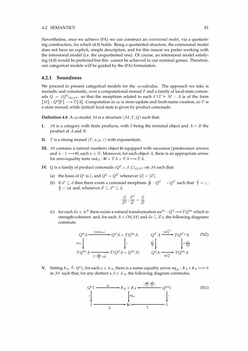
4.2. SEMANTICS 81
Nevertheless, once we achieve (FA) we can construct an extensional model, via a quotient-ing construction, for which (4.8) holds. Being a quotiented structure, the extensional model
does not have an explicit, simple description, and for this reason we prefer working withthe intensional model (i.e. the unquotiented one). Of course, an intensional model satisfy-
ing (4.8) would be preferred but this cannot be achieved in our nominal games. Therefore,
our categorical models will be guided by the (FA) formulation.
4.2.1 Soundness
We proceed to present categorical models for the νρ-calculus. The approach we take is
monadic and comonadic, over a computational monad T and a family of local-state comon-ads Q = (Q~a)~a∈A# , so that the morphism related to each ~a ^ Γ_M : A is of the form
JMK : Q~aJΓK B T JAK. Computation in νρ is store-update and fresh-name creation, so T is
a store monad, while (initial) local state is given by product comonads.
Definition 4.8 A νρ-model M is a structure (M, T,Q) such that:
I. M is a category with finite products, with 1 being the terminal object and A × B theproduct of A and B.
II. T is a strong monad (T, η, µ, τ) with exponentials.
III. M contains a natural numbers object N equipped with successor/predecessor arrowsand
bn : 1 B N, each n ∈ N. Moreover, for each object A, there is an appropriate arrow
for zero-equality tests cndA : N× TA× TAB TA.
IV. Q is a family of product comonads (Q~a, ε, δ, ζ )~a∈A# on M such that:
(a) the basis of Qǫ is 1, and Q~a = Q~a′
whenever [~a] = [~a′],
(b) if ~a′ ⊆ ~a then there exists a comonad morphism ~a~a′ : Q~a B Q~a
′
such that ~aǫ = ε ,
~a~a = id and, whenever ~a′ ⊆ ~a′′ ⊆ ~a,
~a
~a′′;~a′′
~a′=~a
~a′
(c) for each ~aa ∈ A# there exists a natural transformation nu~aa : Q~aB TQ~aawhich isstrength-coherent and, for each A ∈ Ob(M) and ~aa ⊆ ~a′a, the following diagrams
commute.
Q~aA
nuA
��
〈id,nuA〉 // Q~aA× TQ~aaA
τ
��TQ~aaA
T 〈~aa~a ,id〉
// T (Q~aA×Q~aaA)
Q~a′
Anu
~a′aA //
~a′
~a��
TQ~a′aA
T~a′a~aa
��Q~aA
nu~aaA
// TQ~aaA
(N2)
V. Setting AA , Qa1, for each a ∈ AA, there is a name-equality arrow eqA : AA×AA B NinM such that, for any distinct a, b ∈ AA, the following diagram commutes.
Qa1∆ //
!
��
AA × AAeqA
��
Qab1〈aba ,
abb 〉
oo
!
��1 b
0
// N 1b1
oo
(N1)
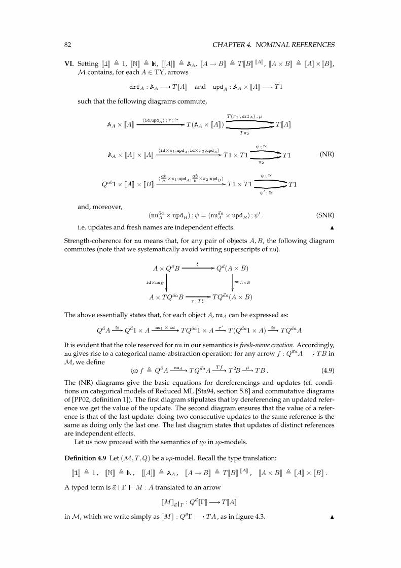
82 CHAPTER 4. NOMINAL REFERENCES
VI. Setting J1K , 1, JNK , N, J[A]K , AA, JA→ BK , T JBK JAK , JA ×BK , JAK×JBK,M contains, for each A ∈ TY, arrows
drfA : AA B T JAK and updA : AA × JAK B T 1
such that the following diagrams commute,AA × JAK〈id,updA〉 ; τ ;∼= // T (AA × JAK)
T (π1 ; drfA) ;µ--
Tπ2
11 T JAKAA × JAK × JAK〈id×π1;updA,id×π2;updA〉 // T 1 × T 1
ψ ;∼=++
π2
33 T 1
Qab1 × JAK × JBK〈aba ×π1;updA,
abb ×π2;updB〉
// T 1 × T 1
ψ ;∼=++
ψ′ ;∼=
33 T 1
(NR)
and, moreover,(nu~aaA × updB) ;ψ = (nu~aaA × updB) ;ψ′ . (SNR)
i.e. updates and fresh names are independent effects. N
Strength-coherence for nu means that, for any pair of objects A,B, the following diagram
commutes (note that we systematically avoid writing superscripts of nu).
A×Q~aB
id×nuB
��
z // Q~a(A×B)
nuA×B
��A× TQ~aaB
τ ;Tz // TQ~aa(A×B)
The above essentially states that, for each object A, nuA can be expressed as:
Q~aA∼=PA Q~a1 ×A
nu1 × idPPPPPPA TQ~aa1 ×A τ ′PA T (Q~aa1 ×A)∼=PA TQ~aaA
It is evident that the role reserved for nu in our semantics is fresh-name creation. Accordingly,
nu gives rise to a categorical name-abstraction operation: for any arrow f : Q~aaAB TB in
M, we define \a℄ f , Q~aAnuAPPPA TQ~aaA
TfPPA T 2BµPA TB . (4.9)
The (NR) diagrams give the basic equations for dereferencings and updates (cf. condi-
tions on categorical models of Reduced ML [Sta94, section 5.8] and commutative diagramsof [PP02, definition 1]). The first diagram stipulates that by dereferencing an updated refer-
ence we get the value of the update. The second diagram ensures that the value of a refer-
ence is that of the last update: doing two consecutive updates to the same reference is thesame as doing only the last one. The last diagram states that updates of distinct references
are independent effects.Let us now proceed with the semantics of νρ in νρ-models.
Definition 4.9 Let (M, T,Q) be a νρ-model. Recall the type translation:
J1K , 1 , JNK , N , J[A]K , AA , JA→ BK , T JBK JAK , JA×BK , JAK × JBK .
A typed term is ~a ^ Γ_M : A translated to an arrow
JMK~a^Γ : Q~aJΓK B T JAK
inM, which we write simply as JMK : Q~aΓ B TA , as in figure 4.3. N
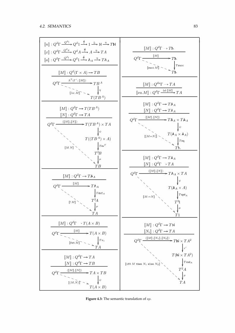
4.2. SEMANTICS 83
JnK : Q~aΓQ~a!PPPA Q~a1
~aǫPA 1
bnPA N ηPA TN
JxK : Q~aΓQ~aπPPPA Q~aA
~aǫPA A
ηPA TA
JaK : Q~aΓQ~a!PPPA Q~a1
~aaPA AA ηPA TAA
JMK : Q~a(Γ ×A)A TB
Q~aΓ
Jλx.MK ))TTTTTTTT
ΛT (z ′ ; JMK) // TB A
η
��T (TBA)
JMK : Q~aΓ A T (TBA)
JNK : Q~aΓ A TA
Q~aΓ
JM NK
!!CC
CC
CC
CC
CC
CC
CC
〈JMK,JNK〉 // T (TBA) × TA
ψ��
T ((TBA) ×A)
T evT
��T 2B
µ
��TB
JMK : Q~aΓ A TAAQ~aΓ
J!MK
$$HH
HH
HH
HH
HH
JMK // TAATdrfA
��T 2A
µ
��TA
JMK : Q~aΓ A T (A×B)
Q~aΓ
JfstMK**UUUUUUUUU
JMK // T (A×B)
Tπ1
��TA
JMK : Q~aΓ A TA
JNK : Q~aΓ A TB
Q~aΓ
J〈M,N〉K **TTTTTTTT〈JMK,JNK〉 // TA× TB
ψ��
T (A×B)
JMK : Q~aΓ A TNQ~aΓ
JsuccMK ))SSSSSSSS
JMK // TNTsucc��
TNJMK : Q~aaΓ A TA
Jνa.MK : Q~aΓ\a℄ JMKPPPPPA TA
JMK : Q~aΓ A TAAJNK : Q~aΓ A TAA
Q~aΓ
J[M=N ]K
%%KK
KK
KK
KK
KK
K
〈JMK,JNK〉 // TAA × TAAψ��
T (AA × AA)
Teq
��TN
JMK : Q~aΓ A TAAJNK : Q~aΓ A TA
Q~aΓ
JM :=NK
AA
AA
AA
AA
AA
AA
A
〈JMK,JNK〉 // TAA × TA
ψ��
T (AA ×A)
TupdA
��T 21
µ
��T 1
JMK : Q~aΓ A TNJNiK : Q~aΓ A TA
Q~aΓ
Jif0 M then N1 else N2K
AA
AA
AA
AA
AA
AA
AA
〈JMK,JN1K,JN2K〉 // TN× TA2
τ ′
��T (N× TA2)
TcndA
��T 2A
µ
��TA
Figure 4.3: The semantic translation of νρ.
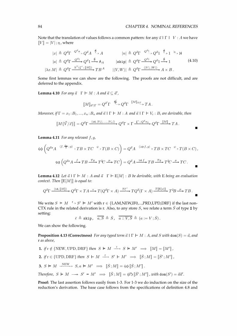
84 CHAPTER 4. NOMINAL REFERENCES
Note that the translation of values follows a common pattern: for any ~a ^ Γ_ V : Awe haveJV K = |V | ; η , where
|x| , Q~aΓQ~aπPPPA Q~aA
~aǫPA A |n| , Q~aΓ
Q~a!PPPA Q~a1~aǫPA 1
bnPA N
|a| , Q~aΓQ~a!PPPA Q~a1
~aaPA AA |skip| , Q~aΓ
Q~a!PPPA Q~a1~aǫPA 1
|λx.M | , Q~aΓΛT (z ′ ; JMK)PPPPPPPPPA TB A |〈V,W 〉| , Q~aΓ
〈|V |, |W |〉PPPPPPPA A×B .
(4.10)
Some first lemmas we can show are the following. The proofs are not difficult, and are
deferred to the appendix.
Lemma 4.10 For any ~a ^ Γ_M : A and ~a ⊆ ~a′,
JMK~a′|Γ = Q~a′
Γ~a′
~aPPA Q~aΓJMK~a|ΓPPPPPA TA .
Moreover, if Γ = x1 :B1, ..., xn :Bn and ~a ^ Γ_M : A and ~a ^ Γ_ Vi : Bi are derivable, then
JM{~V /~x}K = Q~aΓ〈id, |V1|, ..., |Vn|〉PPPPPPPPPPPPA Q~aΓ × Γ
z ′ ;Q~aπ2PPPPPPA Q~aΓJMKPPPA TA .
�
Lemma 4.11 For any relevant f, g,\a℄(Q~aaA 〈f, ~aa~a
; g〉PPPPPPPA TB × TCψPA T (B × C)
)
= Q~aA〈\a℄ f, g〉PPPPPPA TB × TC
ψPA T (B × C) ,\a℄(Q~aaA fPA TBTgPPA T 2C
µPA TC)
= Q~aA\a℄ fPPPA TB
TgPPA T 2CµPA TC .
�
Lemma 4.12 Let ~a ^ Γ_M : A and ~a ^ Γ_E[M ] : B be derivable, with E being an evaluationcontext. Then JE[M ]K is equal to:
Q~aΓ〈id, JMK〉PPPPPPPA Q~aΓ × TA τPA T (Q~aΓ ×A)
Tz ′PPPA TQ~a(Γ ×A)T JE[x]KPPPPPA T 2B
µPA TB .�
We write S ` M rPA S′ ` M ′ with r ∈ {LAM,NEW,IF0,...,PRD,UPD,DRF} if the last non-CTX rule in the related derivation is r. Also, to any store S, we relate a term S of type 1 by
setting:ǫ , skip , a, S , S , a :: V, S , (a := V ; S) .
We can show the following.
Proposition 4.13 (Correctness) For any typed term ~a ^ Γ_M : A, and S with dom(S) = ~a, andr as above,
1. if r /∈ {NEW,UPD,DRF} then S `Mr
−−→ S `M ′ =⇒ JMK = JM ′K ,
2. if r ∈ {UPD,DRF} then S `Mr
−−→ S′ `M ′ =⇒ JS ;MK = JS′ ;M ′K ,
3. S `MNEW
−−−−−→ S, a`M ′ =⇒ JS ;MK = \a℄ JS ;M ′K .
Therefore, S `M −→→ S′ `M ′ =⇒ JS ;MK = \~a′℄ JS′ ;M ′K , with dom(S′) = ~a~a′.
Proof: The last assertion follows easily from 1-3. For 1-3 we do induction on the size of the
reduction’s derivation. The base case follows from the specifications of definition 4.8 and
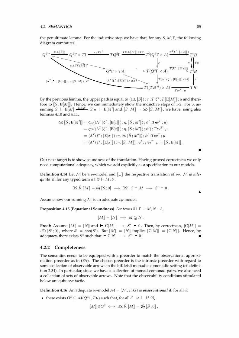
4.2. SEMANTICS 85
the penultimate lemma. For the inductive step we have that, for any S,M,E, the followingdiagram commutes.
Q~aΓ
〈id,JS ;MK〉++WWWWWWWWWWWWWWWWWWWWWWWWWWWW
〈ΛT (z ′ ; JE[x]K) ; η,JS ;MK〉 ;ψ′
//
〈id,JSK〉 // Q~aΓ × T 1τ ; Tz ′
// TQ~aΓT 〈id,JMK〉 ;Tτ // T 2(Q~aΓ ×A)
T 2(z ′ ; JE[x]K)//
µ
��
T 3B
Tµ
��µ
��Q~aΓ × TA
τ //
ΛT (z ′ ; JE[x]K)×id ; τ))RRRRRRRRRRRRRRT (Q~aΓ ×A)
T (ΛT (z ′ ; JE[x]K)×id)
��
T (z ′ ; JE[x]K) // T 2B
µ
��T ((TBA) ×A)
T evT ;µ
// TB
By the previous lemma, the upper path is equal to 〈id, JSK〉 ; τ ;T ζ ′ ;T JE[M ]K ;µ and there-
fore to JS ; E[M ]K. Hence, we can immediately show the inductive steps of 1-2. For 3, as-suming S ` E[M ] NEWPPPPA S, a ` E[M ′] and JS ;MK = \a℄ JS ;M ′K , we have, using also
lemmas 4.10 and 4.11,\a℄ JS ; E[M ′]K = \a℄(〈ΛT (ζ ′ ; JE[x]K) ; η, JS ;M ′K〉 ;ψ′ ;T evT ;µ)
= \a℄(〈ΛT (ζ ′ ; JE[x]K) ; η, JS ;M ′K〉 ;ψ′) ;T evT ;µ
= 〈ΛT (ζ ′ ; JE[x]K) ; η, \a℄ JS ;M ′K〉 ;ψ′ ;T evT ;µ
= 〈ΛT (ζ ′ ; JE[x]K) ; η, JS ;MK〉 ;ψ′ ;T evT ;µ = JS ; E[M ]K .
�
Our next target is to show soundness of the translation. Having proved correctness we only
need computational adequacy, which we add explicitly as a specification to our models.
Definition 4.14 Let M be a νρ-model and J K the respective translation of νρ. M is ade-
quate if, for any typed term ~a ^∅_M :N,
∃S,~b. JMK = \~b℄ JS ; 0K =⇒ ∃S′. ~a`M −→→ S′ ` 0 .N
Assume now our running M is an adequate νρ-model.
Proposition 4.15 (Equational Soundness) For terms ~a ^ Γ_M,N : A,
JMK = JNK =⇒ M / N .
Proof: Assume JMK = JNK and ` C[M ] −→→ S′ ` 0 . Then, by correctness, JC[M ]K =\~a′℄ JS′ ; 0K , where ~a′ = dom(S′). But JMK = JNK implies JC[M ]K = JC[N ]K. Hence, by
adequacy, there exists S′′ such that` C[N ] −→→ S′′ ` 0 . �
4.2.2 Completeness
The semantics needs to be equipped with a preorder to match the observational approxi-
mation preorder as in (FA). The chosen preorder is the intrinsic preorder with regard tosome collection of observable arrows in the biKleisli monadic-comonadic setting (cf. defini-
tion 2.34). In particular, since we have a collection of monad-comonad pairs, we also need
a collection of sets of observable arrows. Note that the observability conditions stipulatedbelow are quite syntactic.
Definition 4.16 An adequate νρ-model M = (M, T,Q) is observational if, for all ~a:
• there exists O~a ⊆ M(Q~a1, TN) such that, for all ~a ^∅_M :N,
JMK∈O~a ⇐⇒ ∃S,~b. JMK = \~b℄ JS ; 0K ,
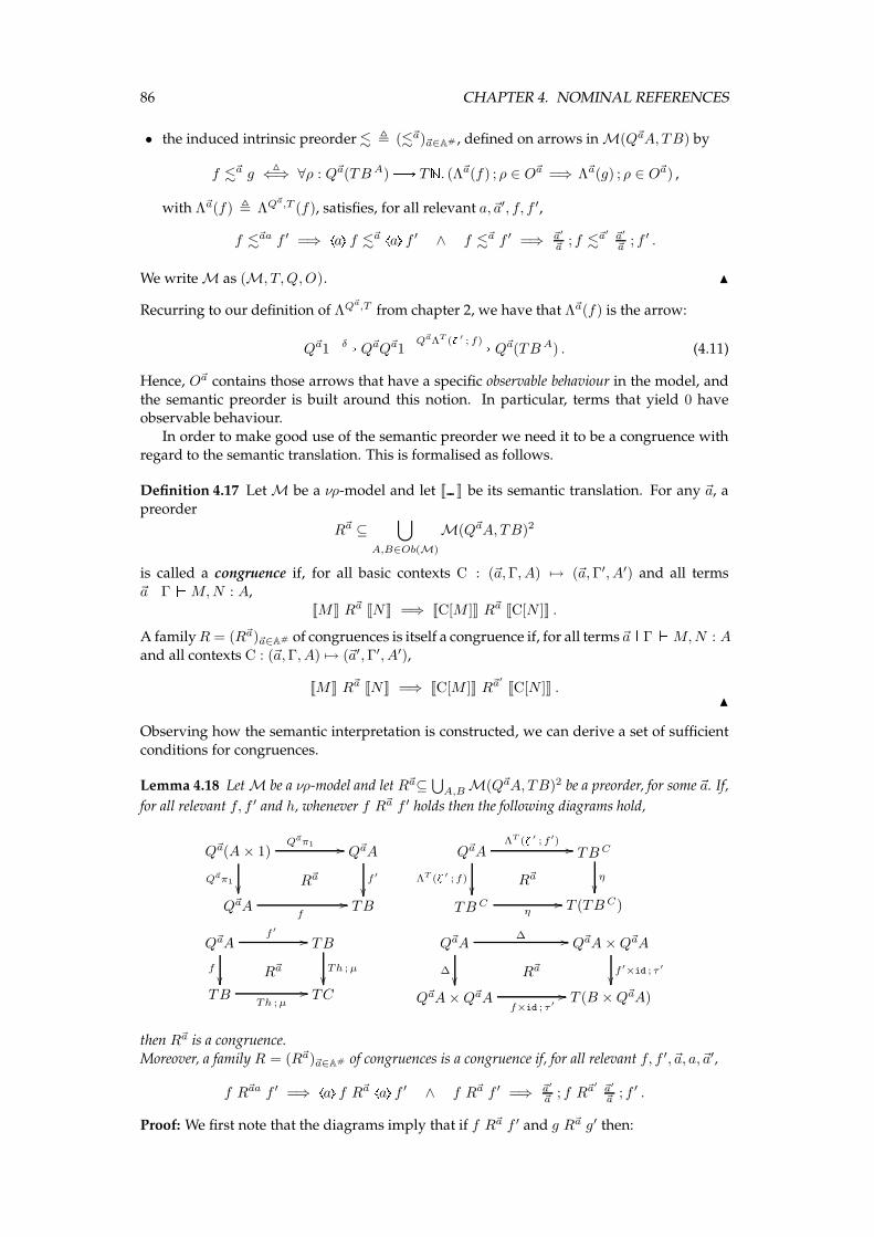
86 CHAPTER 4. NOMINAL REFERENCES
• the induced intrinsic preorder . , (.~a)~a∈A# , defined on arrows in M(Q~aA, TB) by
f .~a g△
⇐⇒ ∀ρ : Q~a(TB A)B TN. (Λ~a(f) ; ρ ∈ O~a =⇒ Λ~a(g) ; ρ ∈ O~a) ,
with Λ~a(f) , ΛQ~a,T (f), satisfies, for all relevant a,~a′, f, f ′,
f .~aa f ′ =⇒ \a℄ f .~a \a℄ f ′ ∧ f .~a f ′ =⇒ ~a′
~a ; f .~a′ ~a′
~a ; f ′ .
We write M as (M, T,Q,O). N
Recurring to our definition of ΛQ~a,T from chapter 2, we have that Λ~a(f) is the arrow:
Q~a1 δPA Q~aQ~a1Q~aΛT (z ′ ; f)PPPPPPPPPA Q~a(TB A) . (4.11)
Hence, O~a contains those arrows that have a specific observable behaviour in the model, and
the semantic preorder is built around this notion. In particular, terms that yield 0 haveobservable behaviour.
In order to make good use of the semantic preorder we need it to be a congruence with
regard to the semantic translation. This is formalised as follows.
Definition 4.17 Let M be a νρ-model and let J K be its semantic translation. For any ~a, a
preorder
R~a ⊆⋃
A,B∈Ob(M)
M(Q~aA, TB)2
is called a congruence if, for all basic contexts C : (~a,Γ, A) 7→ (~a,Γ′, A′) and all terms
~a ^ Γ_M,N : A,JMK R~a JNK =⇒ JC[M ]K R~a JC[N ]K .
A familyR = (R~a)~a∈A# of congruences is itself a congruence if, for all terms~a ^ Γ_M,N : A
and all contexts C : (~a,Γ, A) 7→ (~a′,Γ′, A′),
JMK R~a JNK =⇒ JC[M ]K R~a′
JC[N ]K .N
Observing how the semantic interpretation is constructed, we can derive a set of sufficient
conditions for congruences.
Lemma 4.18 Let M be a νρ-model and let R~a⊆⋃
A,BM(Q~aA, TB)2 be a preorder, for some ~a. If,
for all relevant f, f ′ and h, whenever f R~a f ′ holds then the following diagrams hold,
Q~a(A× 1)Q~aπ1 //
Q~aπ1
��
Q~aA
f ′
��R~a
Q~aAf
// TB
Q~aAΛT (z ′ ; f ′) //
ΛT (z ′ ; f)
��
TBC
η
��R~a
TB Cη
// T (TBC)
Q~aAf ′
//
f
��
TB
Th ;µ
��R~a
TBTh ;µ
// TC
Q~aA∆ //
∆��
Q~aA×Q~aA
f ′×id ; τ ′
��R~a
Q~aA×Q~aAf×id ; τ ′
// T (B ×Q~aA)
then R~a is a congruence.
Moreover, a family R = (R~a)~a∈A# of congruences is a congruence if, for all relevant f, f ′,~a, a,~a′,
f R~aa f ′ =⇒ \a℄ f R~a \a℄ f ′ ∧ f R~a f ′ =⇒ ~a′
~a ; f R~a′ ~a′
~a ; f ′ .
Proof: We first note that the diagrams imply that if f R~a f ′ and g R~a g′ then:
4.2. SEMANTICS 87
• f ; η = ( ∆ ;(ΛT (ζ ′ ;Q~aπ1 ; f) ; η) × id ; τ ′ ;T (id×! ; evT ; η) ;µ ) R~a (f ′ ; η).
• f ;h = (f ; η ;Th ;µ) R~a (f ′ ;h).
• 〈f, g〉 ;ψ = (∆ ; f × id ; τ ′ ;T (id× g ; τ) ;µ) R~a (〈f ′, g〉 ;ψ).
• 〈f ′, g〉 ;ψ = (∆ ; g × id ; τ ′ ;T (id× f ′) ;Tτ ;T 2〈π2, π1〉 ;µ) R~a (〈f ′, g′〉 ;ψ).
• 〈f, g〉 ; τ = (〈f ; η, g〉 ;ψ) R~a (〈f ′, g′〉 ; τ).
• 〈f, g〉 ; τ ′ = (〈f, g ; η〉 ;ψ) R~a (〈f ′, g′〉 ; τ ′).
It then follows that R~a is a congruence, by induction on contexts. Finally, in order to showthat R is a congruence it suffices to show that for all ~a ^ Γ_M,N : A, JMK R~a JNK implies:
• JMK~a′|Γ R~a′ JNK~a′|Γ, for any ~a ⊆ ~a′,
• Jνa.MK R~a′
Jνa.NK, whenever ~a = ~a′a.
But, using also lemma 4.10, we see that these conditions precisely correspond to the condi-tions for congruences. �
It is now straightforward to show that the semantic preorder is a congruence.
Corollary 4.19 Let (M, T,Q~a, O) be an observational νρ-model. Then, (.~a)~a∈A# is a congruence.
Proof: We need only show the four diagrams of the previous lemma, and these are easily ob-
tained from the enrichment properties of the semantic preorder, proven in proposition 2.35.For example, for the first diagram and for general h : A′ B A, we have:
Q~ah ; f = δ ;Q~aε ;Q~ah ;Q~aη ; ℓ ;Tf ;µ
which falls within the first claim of that proposition. �
Assume now that we translate νρ in an observational νρ-model. Then, one direction of (FA)follows immediately form the definition.
Lemma 4.20 (Inequational Soundness) For terms ~a ^ Γ_M,N : A,
JMK . JNK =⇒ M / N .
Proof: Assume JMK .~a JNK and ` C[M ] −→→ S′ ` 0 , so JC[M ]K = \~a′℄ JS′ ; 0K with~a′ = dom(S′). JMK .~a JNK implies JC[M ]K . JC[N ]K , and hence JC[N ]K ∈ Oǫ. Thus, by
observationality and adequacy, there exists S′′ such that` C[N ] −→→ S′′ ` 0 . �
In order to achieve completeness, and hence full-abstraction, we need our semantic transla-
tion to satisfy some definability requirement with regard to the intrinsic preorder.
Definition 4.21 Let (M, T,Q,O) be an observational νρ-model and let J K be the semantic
translation of νρ to M. M satisfies ip-definability if, for all ~a,A,B, there exists D~aA,B ⊆
M(Q~aJAK, T JBK) such that:
• for each f ∈ D~aA,B there exists termM such that JMK = f ,
• for each f, g ∈ M(Q~aJAK, T JBK),
f .~a g ⇐⇒ ∀ρ ∈ D~aA→B,N . (Λ~a(f) ; ρ ∈ O~a =⇒ Λ~a(g) ; ρ ∈ O~a) .
We write M as (M, T,Q,O,D). N
88 CHAPTER 4. NOMINAL REFERENCES
For such a model Mwe achieve full abstraction.
Proposition 4.22 (FA) For terms ~a ^ Γ_M,N : A,
JMK . JNK ⇐⇒ M / N .
Proof: Soundness is by previous lemma. For completeness (⇐=), we do induction on thesize of Γ.
For the base case suppose~a ^∅_M / N and take any ρ ∈ D 1→A,N such thatΛ~a(JMK) ; ρ ∈O~a . Let ρ = J~a ^ y : 1→ A_ L : NK , some L, so Λ~a(JMK) ; ρ is
Λ~a(JMK) ; JLK = δ ;Q~a|λz.M | ; JLK = J(λy.L)(λz.M)K
for some z :1. The latter being in O~a implies that it equals \~b℄ JS ; 0K, some S. Now,M / N
implies (λy.L)(λz.M) / (λy.L)(λz.N) , hence ν~b.(S ; 0) / (λy.L)(λz.N) , by soundness. But
this implies that ~a ` (λy.L)(λz.N) AA S′ ` 0 , so J(λy.L)(λz.N)K ∈ O~a, by correctness.Hence, Λ~a(JNK) ; ρ ∈ O~a, so JMK .~a JNK, by ip-definability.
For the inductive step, if Γ = x :B,Γ′ then
~a ^ Γ_M / N =⇒ ~a ^ Γ′_ λx.M / λx.NIH=⇒ Jλx.MK .~a Jλx.NK
=⇒ JMK = J(λx.M)xK(∗)
.~a J(λx.N)xK = JNK
where (∗) follows from corollary 4.19. �
4.3 The nominal games model
We embark on the adventure of modelling νρ in a category of nominal arenas and strategies.
Our starting point is the category Vt of nominal arenas and total strategies (definition 3.51).Recall that Vt is constructed within the category Nom of nominal sets so, for each type A,
we have an arena AA for references to typeA. Explicitly, AA is the flat arena Aa, with a ∈ AA,defined in (3.1).
The semantics is monadic in a store monad built around a store arena ξ, and comonadic
in an initial state comonad. The store monad is defined on top of the lifting monad (seedefinition 3.68) by use of the side-effect constructor described in section 2.3.3, that is,
TA , ξ −−⊗ (A⊗ ξ)⊥ (i.e. TA = ξ⇒A⊗ ξ).
Now, ξ contains the values assigned to each name (reference), and thus it is of the form
⊗
A∈TY(AA ⇒ JAK)
where JAK is the translation of each typeA. Thus, a recursive definition of the type-translationis not possible because of the following cyclicity.
JA→ BK = JAK −−⊗ (ξ⇒ JBK ⊗ ξ)
ξ =⊗
A(AA ⇒ JAK)
(SE)
Rather, both ξ and the type-translation have to be computed as the least solution to the above
domain equation. By the way, observe that JA→ BK = JAK ⊗ ξ⇒ JBK ⊗ ξ .
4.3.1 Solving the Store Equation
The full form of the store equation (SE) is the following.
J1K = 1 , JNK = N , J[A]K = AA , JA×BK = JAK ⊗ JBK ,
JA→ BK = JAK −−⊗ (ξ⇒ JBK ⊗ ξ) , ξ =⊗
A(AA ⇒ JAK) .
4.3. THE NOMINAL GAMESMODEL 89
This can be solved either as a fixpoint equation in the cpo of nominal arenas or as a domainequation in the PreCpo-enriched category Vt. We follow the latter approach, which provides
themost general notion of canonical solution (andwhich incorporates the solution in the cpoof nominal arenas, analogously to [McC00]). It uses the categorical constructions of [SP82,
Fre90] for solving recursive domain equations, as adapted to games in [McC00].
Definition 4.23 Define the category
C , Vt ×∏
A∈TY
Vt
with objects D of the form (Dξ, DAA∈TY) and arrows f of the form (fξ, fA
A∈TY).Now take F : Cop × C → C to be defined on objects by:
F (D,E) , (ξD,E , JAKD,EA∈TY) ,
where
J1KD,E , 1 JA×BKD,E , JAKD,E ⊗ JBKD,E J[A]KD,E , AAJNKD,E , N JA→ BKD,E , DA −−⊗ (ξE,D ⇒EB ⊗ ξD,E) ξD,E ,
⊗
A∈TY(AA ⇒EA)
and similarly for arrows, with F (f, g) , (ξf,g, JAKf,gA∈TY) . N
Now (SE) has been reduced to:D = F (D,D) (SE∗)
where F is a locally continuous functor wrt the strategy ordering (proposition 3.65), andcontinuous wrt the arena ordering (proposition 3.67). The solution to (SE∗) is given via a
local bilimit construction to the following ω-chain in C.3
Definition 4.24 In C form the sequence (Di)i∈ω takingD0 as below and Di+1 , F (Di, Di).
D0,1 , 1 D0,N , N D0,[A] , AAD0,A→B , 1 D0,A×B , D0,A ⊗D0,B D0,ξ ,
⊗
A(AA ⇒ 0)
Moreover, define arrows ei : DiB Di+1 and eRi : Di+1 B Di by:
e0 , inclD0,D1 , eR0 , projD1,D0, ei+1 , F (eRi , ei) , eRi+1 , F (ei, e
Ri ) .
N
The above inclusion and projection arrows are defined componentwise. In fact, there is a
hidden lemma in the definition which allows us to define the projection arrow, namely that
D0 E1 D1 (which means D0,ξ E1 D1,ξ andD0,A E1 D1,A for all A).Thus, we have formed the ω-chain ∆:
D0e0 // D1
e1 // D2e2 // D3
e3 // · · · (∆)
We now show that ∆ is a E-increasing sequence of objects and embeddings, and proceed tothe main result.
3Recall that we call an arrow e : AB B an embedding if there exists eR : B B A such that
e ; eR = idA ∧ eR ; e ⊑ idB .
Given an ω-chain ∆ = (Di, ei)i∈ω of objects and embeddings, a cone for ∆ is an object D together with a family(ηi : Di B D)i∈ω of embeddings such that, for all i ∈ ω, ηi = ei ; ηi+1. Such a cone is a local bilimit for ∆ if,for all i ∈ ω,
ηRi ; ηi ⊑ ηRi+1 ; ηi+1 ∧G
i∈ω(ηRi ; ηi) = idD .
90 CHAPTER 4. NOMINAL REFERENCES
Lemma 4.25 For (ei, eRi )i∈ω as above and any i ∈ ω,
ei = inclDi,Di+1 ∧ eRi = projDi+1,Di.
Proof: Doing induction on i we can show that Di E1 Di+1, all i ∈ ω, and that the aboveequalities hold. The base case is true by definition; the inductive step follows from proposi-
tion 3.67. �
Theorem 4.26 We obtain a local bilimit (D∗, ηii∈ω) for ∆ by taking:
D∗ ,⊔
iDi , ηi , inclDi,D∗ (each i ∈ ω).
Hence, idD∗ : F (D∗, D∗)B D∗ is a minimal invariant for F .
Proof: First, note that D0 E1 Di, for all i ∈ ω, implies that all Di’s share the same initial
moves, and hence Di E1 D∗. Thus, for each i ∈ ω, we can define ηRi , projD∗,Di
, andhence each ηi is an embedding. We now need to show the following.
1. (D∗, ηii∈ω) is a cone for ∆,
2. for all i ∈ ω, ηRi ; ηi ⊑ ηRi+1 ; ηi+1 ,
3.⊔
i∈ω(ηRi ; ηi) = idD∗ .
For 1, we nts that, for any i, inclD1,D∗ = inclDi,Di+1 ; inclDi+1,D∗ , which follows from
(TRN). For 2 we essentially nts that idDi⊆ idDi+1 , and for 3 that
⋃
i idDi= idD∗ ; these are
both straightforward.From the local bilimit (D∗, ηi
i∈ω) we obtain a minimal invariant α : F (D∗, D∗) B D∗ by
taking (see e.g. [Abr07]):
α ,⊔
iαi , αi , F (ηi, η
Ri ) ; ηi+1
prop. 3.67= projF (D∗,D∗),Di+1
; inclDi+1,D∗ .
Moreover, D∗ = F (D∗, D∗) by the Tarski-Knaster theorem, and therefore αi = ηRi+1 ; ηi+1 ,which implies α = idD∗ . �
Thus, D∗ is the canonical solution to D = F (D,D), and in particular it solves:
DA→B = DA −−⊗ (Dξ ⇒DB ⊗Dξ)
Dξ =⊗
A(AA ⇒DA) .
Definition 4.27 (ξ, ⊛ and JAK) LetD∗ be as in the previous theorem. Define the store arenaξ and, for each type A, the translation JAK of A by:
ξ , D∗ξ , JAK , D∗
A .N
The arena ξ and the translation of compound types are given explicitly in the following
figure. ξ is depicted by means of unfolding it to⊗
A(AA ⇒ JAK) : it consists of an initialmove ⊛ which justifies each name-question a ∈ AA, all types A, with the answer to the
latter being the denotation of A (and modelling the stored value of a). Note that we reserve
the symbol “⊛” for the initial move of ξ. ⊛-moves in type-translations can be seen as openinga new store.
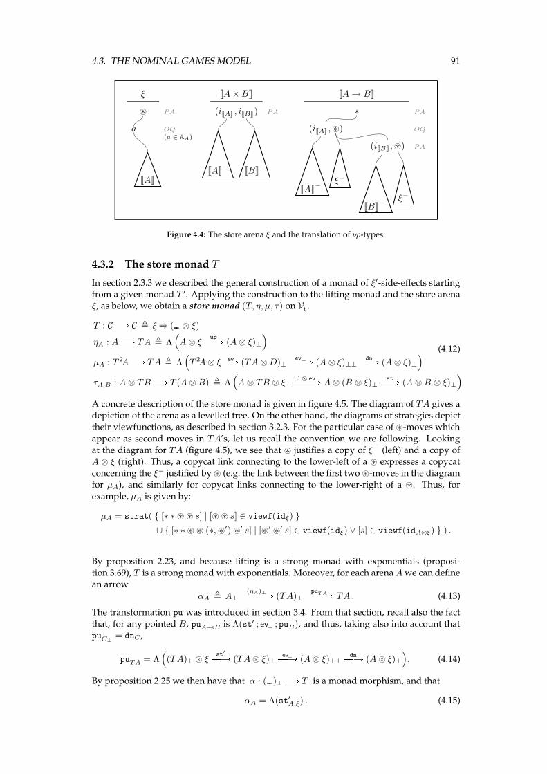
4.3. THE NOMINAL GAMESMODEL 91
ξ
⊛ PA
a OQ(a ∈ AA)
JAK
JA×BK
(iJAK , iJBK) PA
JAK− JBK−
JA→ BK
∗ PA
(iJAK ,⊛) OQ
JAK−
ξ−
(iJBK ,⊛) PA
JBK−
ξ−
Figure 4.4: The store arena ξ and the translation of νρ-types.
4.3.2 The store monad T
In section 2.3.3 we described the general construction of a monad of ξ′-side-effects startingfrom a given monad T ′. Applying the construction to the lifting monad and the store arena
ξ, as below, we obtain a store monad (T, η, µ, τ) on Vt.
T : C B C , ξ⇒ ( ⊗ ξ)
ηA : AB TA , Λ(
A⊗ ξupPPA (A⊗ ξ)⊥
)
µA : T 2AB TA , Λ(
T 2A⊗ ξ evPA (TA⊗D)⊥ev⊥PPPA (A⊗ ξ)⊥⊥
dnPPA (A⊗ ξ)⊥
)
τA,B : A⊗ TBB T (A⊗B) , Λ(
A⊗ TB ⊗ ξid ⊗ evPPPPPA A⊗ (B ⊗ ξ)⊥
stPPA (A⊗B ⊗ ξ)⊥
)
(4.12)
A concrete description of the store monad is given in figure 4.5. The diagram of TA gives a
depiction of the arena as a levelled tree. On the other hand, the diagrams of strategies depicttheir viewfunctions, as described in section 3.2.3. For the particular case of ⊛-moves which
appear as second moves in TA’s, let us recall the convention we are following. Looking
at the diagram for TA (figure 4.5), we see that ⊛ justifies a copy of ξ− (left) and a copy ofA ⊗ ξ (right). Thus, a copycat link connecting to the lower-left of a ⊛ expresses a copycat
concerning the ξ− justified by ⊛ (e.g. the link between the first two ⊛-moves in the diagramfor µA), and similarly for copycat links connecting to the lower-right of a ⊛. Thus, for
example, µA is given by:
µA = strat( { [∗ ∗ ⊛ ⊛ s] | [⊛ ⊛ s] ∈ viewf(idξ) }
∪ { [∗ ∗ ⊛ ⊛ (∗,⊛′) ⊛′ s] | [⊛′ ⊛′ s] ∈ viewf(idξ) ∨ [s] ∈ viewf(idA⊗ξ) } ) .
By proposition 2.23, and because lifting is a strong monad with exponentials (proposi-
tion 3.69), T is a strong monad with exponentials. Moreover, for each arenaAwe can definean arrow
αA , A⊥(ηA)⊥PPPPPA (TA)⊥
puT APPPPA TA . (4.13)
The transformation pu was introduced in section 3.4. From that section, recall also the fact
that, for any pointed B, puA−−⊗B is Λ(st′ ; ev⊥ ; puB), and thus, taking also into account thatpuC⊥
= dnC ,
puTA = Λ(
(TA)⊥ ⊗ ξst
′PPA (TA⊗ ξ)⊥ev⊥PPA (A⊗ ξ)⊥⊥
dnPPA (A⊗ ξ)⊥
)
. (4.14)
By proposition 2.25 we then have that α : ( )⊥ B T is a monad morphism, and that
αA = Λ(st′A,ξ) . (4.15)

92 CHAPTER 4. NOMINAL REFERENCES
TA
∗ PA
⊛ OQ
ξ−
(iA,⊛) PA
A−ξ−
TATf : // TB∗ OQ
∗ PA
⊛ OQ
⊛ PQ
(iA,⊛) OA
(iB,⊛) PAf
AηA : // TAiA OQ
∗ PA
⊛ OQ
(iA,⊛) PA
T 2AµA : // TA∗ OQ
∗ PA
⊛ OQ
⊛ PQ
(∗,⊛) OA
⊛ PQ
A⊗ TBτA,B : // T (A⊗B)
(iA, ∗) OQ
∗ PA
⊛ OQ
⊛ PQ
(iB,⊛) OA
(iA, iB,⊛) PA
Figure 4.5: The store monad (T, η, µ, τ ) for νρ.
4.3.3 Obtaining the νρ-model
Let us recapitulate the structure we have constructed thus far to the effect of obtaining aνρ-model in Vt. Our numbering below follows that of definition 4.8.
I. Vt is a category with finite products (proposition 3.57).
II. The store monad T is a strong monad with exponentials.
III. Vt contains adequate structure for numerals.
IV. There is a family (Q~a, ε, δ, ζ )~a∈A# of product comonads, with each Q~a having basis A~a(see section 3.4.2), which fulfills specifications (a,b). There are also fresh-name construc-
tors,new~aa : Q~aB (Q~aa)⊥ ,
given in section 3.4.3, which satisfy (N2).
V. There are name-equality arrows, eqA for each type A, making the (N1) diagram com-
mute (section 3.4.2).
From newwe can obtain a fresh-name transformation for the store monad.
Definition 4.28 For each ~aa ∈ A#, define a natural transformation nu~aa : Q~aB TQ~aa by:
nu~aaA , Q~aAnewAPPPA (Q~aaA)⊥
αQ~aaAPPPPPA TQ~aaA .
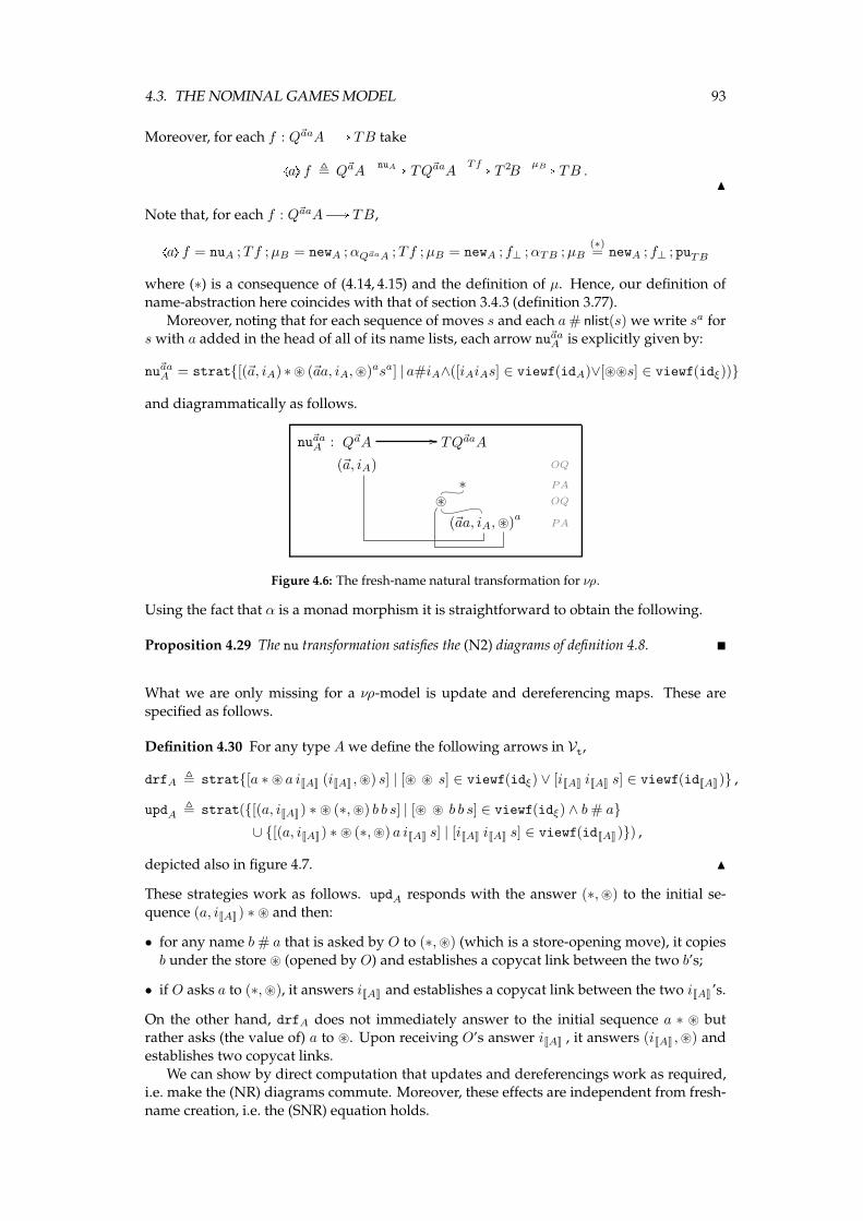
4.3. THE NOMINAL GAMESMODEL 93
Moreover, for each f : Q~aaAB TB take\a℄ f , Q~aAnuAPPPA TQ~aaA
TfPPA T 2BµBPPA TB .
N
Note that, for each f : Q~aaAB TB,\a℄ f = nuA ;Tf ;µB = newA ;αQ~aaA ;Tf ;µB = newA ; f⊥ ;αTB ;µB(∗)= newA ; f⊥ ; puTB
where (∗) is a consequence of (4.14, 4.15) and the definition of µ. Hence, our definition of
name-abstraction here coincides with that of section 3.4.3 (definition 3.77).
Moreover, noting that for each sequence of moves s and each a# nlist(s) we write sa fors with a added in the head of all of its name lists, each arrow nu~aaA is explicitly given by:
nu~aaA = strat{[(~a, iA) ∗⊛ (~aa, iA,⊛)asa] | a#iA∧([iAiAs] ∈ viewf(idA)∨[⊛⊛s] ∈ viewf(idξ))}
and diagrammatically as follows.
Q~aAnu~aaA : // TQ~aaA
(~a, iA) OQ
∗ PA
⊛ OQ
(~aa, iA,⊛)a
PA
Figure 4.6: The fresh-name natural transformation for νρ.
Using the fact that α is a monad morphism it is straightforward to obtain the following.
Proposition 4.29 The nu transformation satisfies the (N2) diagrams of definition 4.8. �
What we are only missing for a νρ-model is update and dereferencing maps. These are
specified as follows.
Definition 4.30 For any type Awe define the following arrows in Vt,
drfA , strat{[a ∗ ⊛ a iJAK (iJAK ,⊛) s] | [⊛ ⊛ s] ∈ viewf(idξ) ∨ [iJAK iJAK s] ∈ viewf(idJAK)} ,
updA , strat({[(a, iJAK) ∗ ⊛ (∗,⊛) b b s] | [⊛ ⊛ b b s] ∈ viewf(idξ) ∧ b# a}
∪ {[(a, iJAK) ∗ ⊛ (∗,⊛) a iJAK s] | [iJAK iJAK s] ∈ viewf(idJAK)}) ,
depicted also in figure 4.7. N
These strategies work as follows. updA responds with the answer (∗,⊛) to the initial se-
quence (a, iJAK) ∗ ⊛ and then:
• for any name b# a that is asked by O to (∗,⊛) (which is a store-opening move), it copies
b under the store ⊛ (opened by O) and establishes a copycat link between the two b’s;
• if O asks a to (∗,⊛), it answers iJAK and establishes a copycat link between the two iJAK ’s.
On the other hand, drfA does not immediately answer to the initial sequence a ∗ ⊛ butrather asks (the value of) a to ⊛. Upon receiving O’s answer iJAK , it answers (iJAK ,⊛) and
establishes two copycat links.
We can show by direct computation that updates and dereferencings work as required,i.e. make the (NR) diagrams commute. Moreover, these effects are independent from fresh-
name creation, i.e. the (SNR) equation holds.
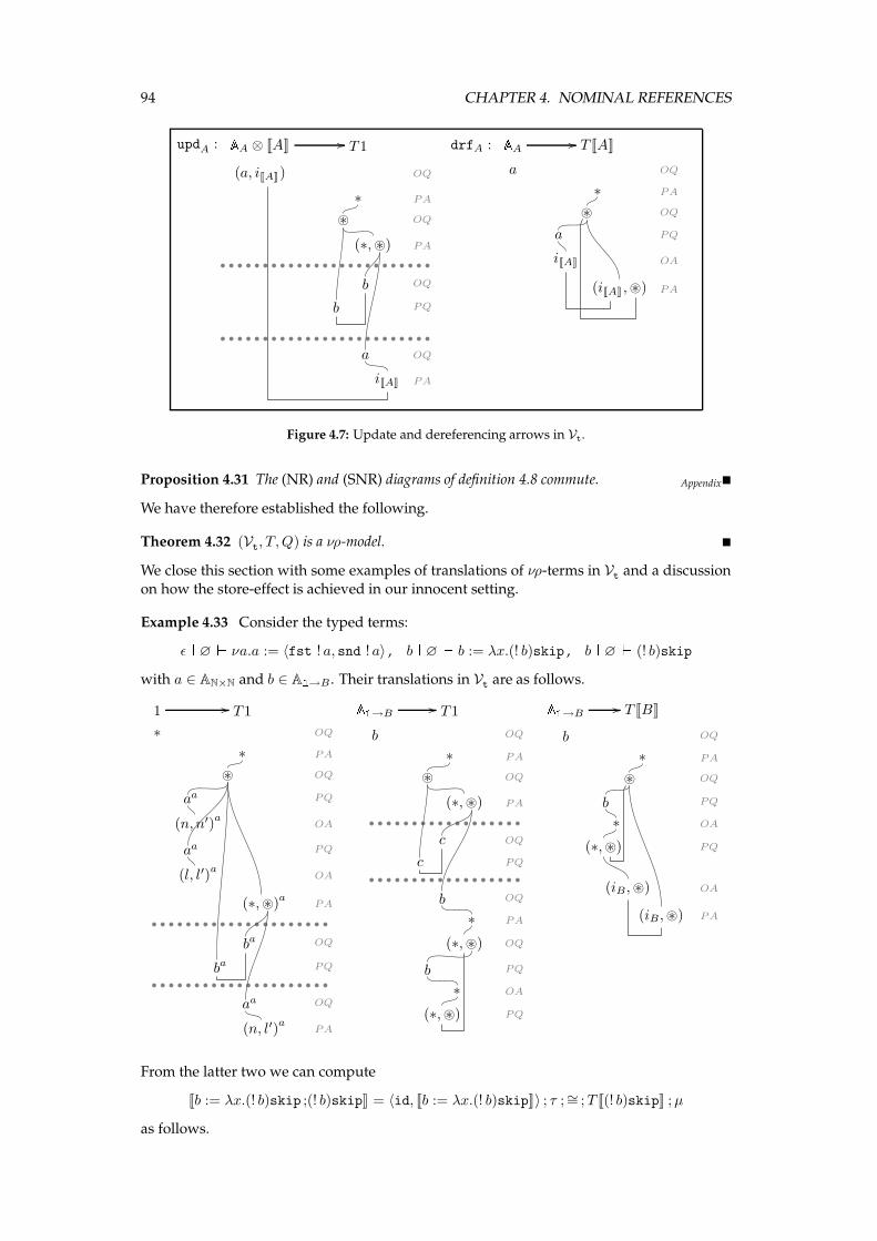
94 CHAPTER 4. NOMINAL REFERENCESAA ⊗ JAKupdA : // T 1
(a, iJAK) OQ
∗ PA
⊛ OQ
(∗,⊛) PA
b OQ
b PQ
a OQ
iJAK PA
AAdrfA : // T JAK
a OQ
∗ PA
⊛ OQ
a PQ
iJAK OA
(iJAK ,⊛) PA
Figure 4.7: Update and dereferencing arrows in Vt.
Proposition 4.31 The (NR) and (SNR) diagrams of definition 4.8 commute. Appendix�
We have therefore established the following.
Theorem 4.32 (Vt, T,Q) is a νρ-model. �
We close this section with some examples of translations of νρ-terms in Vt and a discussion
on how the store-effect is achieved in our innocent setting.
Example 4.33 Consider the typed terms:
ǫ ^∅_ νa.a := 〈fst ! a, snd ! a〉 , b ^∅_ b := λx.(! b)skip , b ^∅_ (! b)skip
with a ∈ AN×N and b ∈ A1→B . Their translations in Vt are as follows.
1 // T 1
∗ OQ
∗ PA
⊛ OQ
aa PQ
(n, n′)a
OA
aa PQ
(l, l′)a
OA
(∗,⊛)a PA
ba OQ
ba PQ
aa OQ
(n, l′)a
PA
A1→B// T 1
b OQ
∗ PA
⊛ OQ
(∗,⊛) PA
c OQ
c PQ
b OQ
∗ PA
(∗,⊛) OQ
b PQ
∗ OA
(∗,⊛) PQ
A1→B// T JBK
b OQ
∗ PA
⊛ OQ
b PQ
∗ OA
(∗,⊛) PQ
(iB,⊛) OA
(iB,⊛) PA
From the latter two we can compute
Jb := λx.(! b)skip ;(! b)skipK = 〈id, Jb := λx.(! b)skipK〉 ; τ ;∼= ;T J(! b)skipK ;µ
as follows.
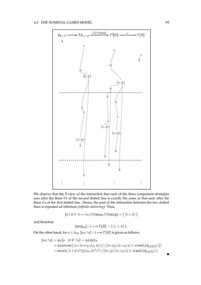
4.3. THE NOMINAL GAMESMODEL 95A1→B... // TA1→B
T J(! b)skipK // T 2JBKµ // T JBK
b
∗
∗
∗
⊛
⊛
⊛
(b,⊛)
(∗,⊛)
⊛
b
b
b
∗
∗
∗
(∗,⊛)
(∗,⊛)
(∗,⊛)
b
b
b
b
b
b
......
......
We observe that the P-view of the interaction that each of the three component strategies
sees after the three b’s of the second dotted line is exactly the same as that seen after thethree b’s of the first dotted line. Hence, the part of the interaction between the two dotted
lines is repeated ad infinitum (infinite chattering). Thus,
Jb ^∅_ b := λx.(! b)skip ;(! b)skipK = { [b ∗ ⊛] }
and therefore
JstopBK : 1 B T JBK = { [∗ ∗ ⊛] } .
On the other hand, for a ∈ AB , Jνa. ! aK : 1B T JBK is given as follows.
Jνa. ! aK = \a℄ Ja ^∅_ ! aK = \a℄ drfB= \a℄(strat{ [a ∗ ⊛ a iB (iB,⊛) s] | [(⊛, iB) (⊛, iB) s] ∈ viewf(idξ⊗JBK) })
= strat{ [∗ ∗ ⊛ aaiaB(iB,⊛)asa] | [(⊛, iB) (⊛, iB) s] ∈ viewf(idξ⊗JBK) }�
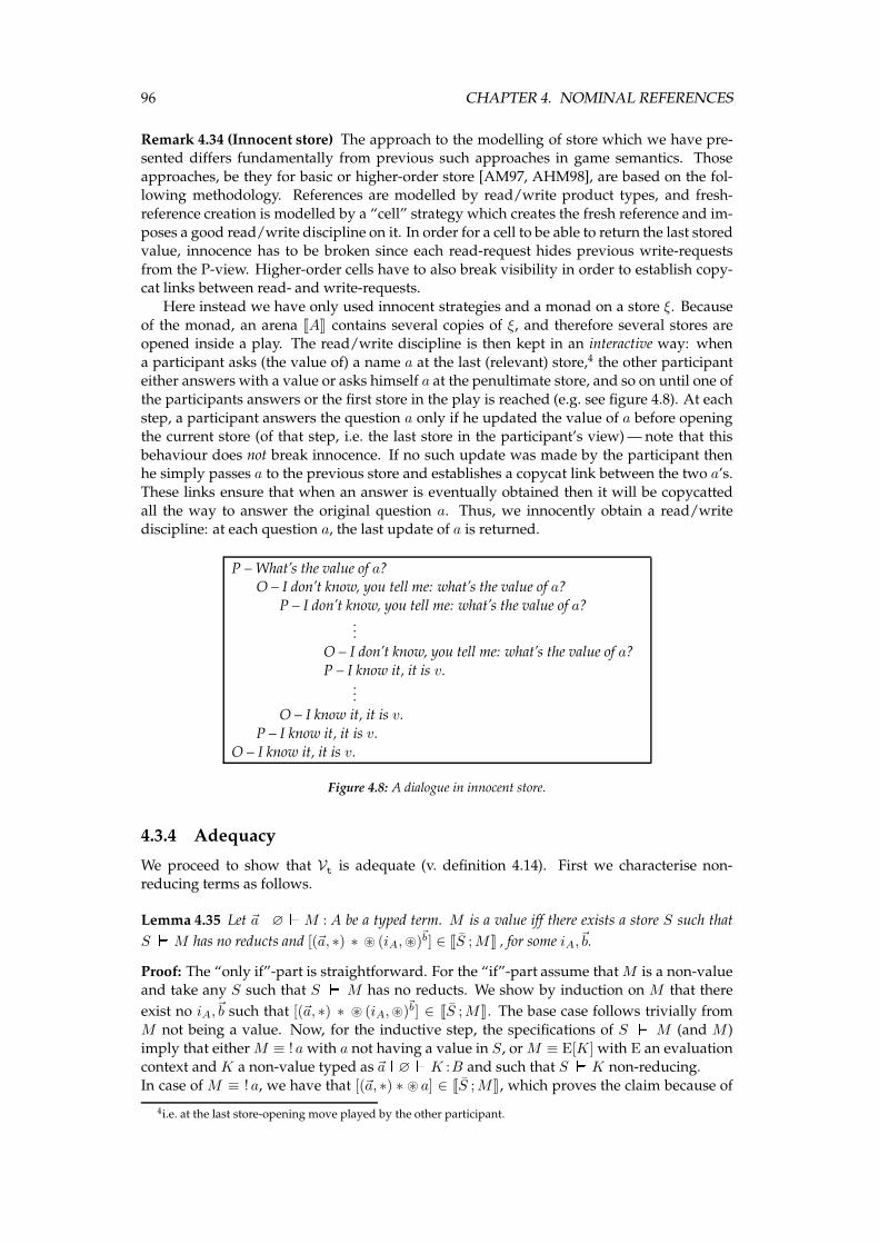
96 CHAPTER 4. NOMINAL REFERENCES
Remark 4.34 (Innocent store) The approach to the modelling of store which we have pre-sented differs fundamentally from previous such approaches in game semantics. Those
approaches, be they for basic or higher-order store [AM97, AHM98], are based on the fol-lowing methodology. References are modelled by read/write product types, and fresh-
reference creation is modelled by a “cell” strategy which creates the fresh reference and im-
poses a good read/write discipline on it. In order for a cell to be able to return the last storedvalue, innocence has to be broken since each read-request hides previous write-requests
from the P-view. Higher-order cells have to also break visibility in order to establish copy-cat links between read- and write-requests.
Here instead we have only used innocent strategies and a monad on a store ξ. Because
of the monad, an arena JAK contains several copies of ξ, and therefore several stores areopened inside a play. The read/write discipline is then kept in an interactive way: when
a participant asks (the value of) a name a at the last (relevant) store,4 the other participanteither answers with a value or asks himself a at the penultimate store, and so on until one of
the participants answers or the first store in the play is reached (e.g. see figure 4.8). At each
step, a participant answers the question a only if he updated the value of a before openingthe current store (of that step, i.e. the last store in the participant’s view)— note that this
behaviour does not break innocence. If no such update was made by the participant thenhe simply passes a to the previous store and establishes a copycat link between the two a’s.
These links ensure that when an answer is eventually obtained then it will be copycatted
all the way to answer the original question a. Thus, we innocently obtain a read/writediscipline: at each question a, the last update of a is returned.
P – What’s the value of a?O – I don’t know, you tell me: what’s the value of a?
P – I don’t know, you tell me: what’s the value of a?...
O – I don’t know, you tell me: what’s the value of a?
P – I know it, it is v....
O – I know it, it is v.
P – I know it, it is v.
O – I know it, it is v.
Figure 4.8: A dialogue in innocent store.
4.3.4 Adequacy
We proceed to show that Vt is adequate (v. definition 4.14). First we characterise non-reducing terms as follows.
Lemma 4.35 Let ~a ^∅_M :A be a typed term. M is a value iff there exists a store S such that
S `M has no reducts and [(~a, ∗) ∗ ⊛ (iA,⊛)~b] ∈ JS ;MK , for some iA,~b.
Proof: The “only if”-part is straightforward. For the “if”-part assume thatM is a non-valueand take any S such that S ` M has no reducts. We show by induction on M that there
exist no iA,~b such that [(~a, ∗) ∗ ⊛ (iA,⊛)~b] ∈ JS ;MK. The base case follows trivially from
M not being a value. Now, for the inductive step, the specifications of S ` M (and M )
imply that eitherM ≡ ! awith a not having a value in S, orM ≡ E[K] with E an evaluationcontext and K a non-value typed as ~a ^∅_K :B and such that S ` K non-reducing.
In case ofM ≡ ! a, we have that [(~a, ∗) ∗ ⊛ a] ∈ JS ;MK, which proves the claim because of
4i.e. at the last store-opening move played by the other participant.
4.3. THE NOMINAL GAMESMODEL 97
determinacy. On the other hand, ifM ≡ E[K] then, as in proof of proposition 4.13, we havethat
JS ;MK = 〈Λ(ζ ′ ; JE[x]K), JS ;KK〉 ; τ ;T ev ;µ = 〈id, JS ;KK〉 ; τ ;T (ζ ′ ; JE[x]K) ;µ
By IH, there are no iB,~c such that [(~a, ∗) ∗ ⊛ (iB,⊛)~c] ∈ JS ;KK, which implies that there are
no iA,~b such that [(~a, ∗) ∗ ⊛ (iA,⊛)~b] ∈ JS ;MK. �
Because of the previous result, in order to show adequacy it will suffice to show that, when-
ever JMK = \~b℄ JS ; 0K, there is no infinite reduction sequence starting from ~a`M . We will
carry out the following reasoning.
• Firstly, since the calculus without DRF reductions is strongly normalising— this is in-
herited from strong normalisation of the sν-calculus— it suffices to show there is noreduction sequence starting from ~a ` M and containing infinitely many DRF reduc-
tion steps.
• In fact, the problem can be further reduced to showing that, whenever [(~a, ∗)∗⊛ (0,⊛)~b] ∈
JMK, there is no reduction sequence starting from ~a ` M and containing infinitely
many NEW reduction steps. But the latter clearly holds, since M cannot create more
than |~b| fresh names in that case, because of correctness.
The reduction to this simpler problem is achieved as follows. For each term M , we
construct a term M ′ by adding immediately before each dereferencing in M a fresh-name construction. The result is that, whenever there is a sequence with infinitely
many DRF’s starting from S ` M , there is a sequence with infinitely many NEW’sstarting from S `M ′. The reduction is completed by finally showing that, whenever
we have [(~a, ∗) ∗ ⊛ (0,⊛)~b] ∈ JMK, we also have [(~a, ∗) ∗ ⊛ (0,⊛)
~b′] ∈ JM ′K.
The crucial step in the proof is the reduction to “the simpler problem”, and particularly
showing the connection between JMK and JM ′K described above. The latter can be carried
out by using the intrinsic preorder on strategies and showing O-adequacy (lemma 4.62):adequacy can then be derived fromO-adequacy. Nevertheless, a direct proof is always useful
(and more fun). We present such a proof in the remainder of this section.
In the following discussion we will be using κ for a νρ-type. We start with a definition.
Definition 4.36 Let κ ∈ TY. For any termM , we define:
κ#M ⇐⇒ ∀a ∈ Aκ. a#M .
For κ#M , we define (M) κ© inductively by:
(x) κ© , x , (a) κ© , a , ... (λx.N) κ© , λx.(N) κ© , (M N) κ© , (M) κ©(N) κ© , ...
and (!N) κ© , νc. !(N) κ©, with c ∈ Aκ. N
Note that a#M means that a does not appear, neither free nor bound, insideM . Our next
target is to show that if κ#M then J(M) κ©K does not use names of type κ. What we mean by
“non-usage” of names is defined formally below (recall the �-quantifier from page 17 andthe notation s = snlist(s) from page 43).
Definition 4.37 Let σ be a strategy. We say that the type κ is essentially fresh for σ, κess
# σ if,
for any a ∈ Aκ,∀s. [s] ∈ σ =⇒ � b. [s(a b) [ nlist(s)] ∈ σ
N
For economy, we let
(a b)[s , s(a b) [ nlist(s) .
98 CHAPTER 4. NOMINAL REFERENCES
What the previous definition is essentially saying is that κess
#σ iff σ does not really use names
of type κ, even though it may be introducing them.There is an alternative definition of essential freshness for strategies, which involves only
viewfunctions.
Proposition 4.38 For any strategy σ, κess
# σ iff, for any a ∈ Aκ,
∀s. [s] ∈ viewf(σ) =⇒ � b. [(a b)[s] ∈ σ .
Proof: Suppose the condition holds and let us pick such an a and some [s] ∈ σ ; we need to
show that � b. [(a b)[s] ∈ σ. We do induction on |s|, taking as base case |s| = 0which is trivial.
For the inductive step, let s = s−x. If x an O-move then � b. [(a b)[s] ∈ σ by contingencycompleteness and the IH. On the other hand, if x a P-move and psq 6= s then, for any fresh b,
[(a b)[(s−)], [p(a b)[sq] ∈ σ by IH and the hypothesis. By lemma 3.38, it suffices to show that(a b)[s is a play. For the latter, we need only check the Name Conditions. (NC3) and (NC2’)
clearly hold, since (a b)[s−, p(a b)[sq are plays. For (NC1), if nlist((a b)[x) contains some new
name c and c 6= b, then c# s− since s is a play, so c# (a b)[s−. If c = b then a# s− since s aplay, ∴ c# (a b)[s− as bwas chosen fresh. �
We can now show the following enrichment properties for essential freshness.
Lemma 4.39 For any relevant σ, τ , if κess
# σ, τ then:
• κess
# σ ; τ ,
• κess
# σ⊥,
• κess
# Λ(σ),
• κess
# 〈σ, τ〉.
Proof: For the first claim we have that [s ; t] ∈ σ ; τ implies that, for any fresh b, [(a b)[s] ∈ σ
and [(a b)[t] ∈ τ . Clearly, (a b)[s ` (a b)[t. Moreover, the fresh-name conditions (C1-2)
still hold: the only thing that could go wrong would be b being introduced at some point
in (a b)[s, say, without being fresh at the respective point in t, which can’t happen as b ischosen fresh.
The other claims follow easily from the previous proposition, and the definitions of these
constructions on viewfunctions. �
Corollary 4.40 For any termM ,
• κ#M =⇒ κess
# JMK,
• κ#M =⇒ κess
# J(M) κ©K.
Proof: Both claims are proven by induction onM . For the first claim, we simply use the fact
that κess
# σ for any strategy σ that does not introduce any names of type κ.
For the second claim, we also use the previous lemma, yet the case ofM ≡ !N needs some
extra attention. By IH we have that κess
# J(N) κ©K, while we know that
J(M) κ©K = nuΓ ;T ~ac~a ;T J!(N) κ©K ;µ
with c ∈ Aκ and M typed in environment ~a^Γ. By previous lemma we have that κess
#
T J!(N) κ©K ;µ, and hence it suffices to show that κess
# nu ;T ~ac~a . We have that:
viewf(nu ;T ~ac~a ) = {[(~a, iΓ) ∗ ⊛ (~a, iΓ,⊛)c sc] | [iΓ iΓ s] ∈ viewf(idJΓK)∨[⊛ ⊛ s] ∈ viewf(idξ)}
4.3. THE NOMINAL GAMESMODEL 99
From the above we observe that, for any a ∈ Aκ, any [s] ∈ viewf(nu ;T ~ac~a ) and any fresh b,[(a b)[s] ∈ nu ;T ~ac~a , as required. �
A consequence of essential freshness is that if κess
# σ then we can delete all κ-name introduc-
tions from σ and still have a strategy.
Definition 4.41 For any play s, define srκ to be swith all names of type κ removed from its
name lists. Take then, for each strategy σ,
σrκ , {[srκ] | [s] ∈ σ} .N
Lemma 4.42 For any strategy σ, if κess
# σ then:
1. if [s] ∈ σ then srκ is a play,
2. if [s1], [s2] ∈ σ, (S(si) \ S(sirκ)) ∩ S(si) = ∅ and [s1rκ] = [s2
rκ] then [s1] = [s2],
3. σrκ is a strategy.
Proof: For 1, we only need to check the Name Conditions still hold, and in particular only(NC2’), as the other two trivially do. So let x be a P-move in srκ and let a ∈ S(x) such that
a # psrκ
<xq. If a /∈ Aκ then a ∈ nlist(x); the case a ∈ Aκ is not possible since then we would
have [(a b)[s] ∈ σ breaking (NC2’), any fresh b.For 2, we do induction on |s1| = |s2|; the base case is trivial. For the inductive step, if |s1|is even then, by IH, [s−1 ] = [s−2 ] and hence, by determinacy, [s1] = [s2]. Finally, if si = s−i xiwith xi an O-move then, by IH, [s−1 ] = [s−2 ]. Now using the condition on supports and the
strong support lemma we obtain [s−1 x1] = [s−2 x2] and thus, by (NC3), [s1] = [s2].
We now show σrκ is a strategy. Prefix closure and contingency completeness are obvious.For determinacy, take even-length [s1x1], [s2x2] ∈ σrκ with sixi = (s′ix
′i)
rκ and [s′ix′i] ∈
σ, and assume [s1] = [s2]. As κ#σ, we can choose s′ix′i in such a way that the names in
S(s′ix′i) \ S(sixi) are fresh for s′ix
′i, and hence, by 2, [s′1] = [s′2]. Then, by determinacy of σ,
[s′1x′1] = [s′2x
′2], which implies [s1x1] = [s2x2]. Finally, for innocence, let [s1x1], [s2] ∈ σrκ
with s1x1 = (s′1x′1)
rκ, s2 = s′2rκ and [s′1x
′1], [s
′2] ∈ σ, and assume [ps1q] = [ps2q]. Then, as
before, we may assume [ps′1q] = [ps′2q] and therefore [s′2x′2] ∈ σ, for some [ps′2x
′2q] = [ps′1x
′1q].
We then have [s2x′2
rκ] ∈ σrκ and [ps1x1q] = [ps2x′2rκq]. �
We need a last lemma before proving adequacy.
Lemma 4.43 For any termM , if κess
#M then JMK ⊆ J(M) κ©Krκ.
Proof: We do induction onM . The base case is encompassed in the case ofM ≡ (M) κ©, in
which case srκ = s for any [s] ∈ JMK and the claim trivially holds. For the inductive step, asJ(M) κ©Krκ is a strategy by previous lemma, it suffices to show that
viewf(JMK) ⊆ {[srκ] | [s] ∈ J(M) κ©K}
We show some characteristic cases:
• M ≡ λx.N . Let [s1 ; s2] ∈ viewf(JMK), where JMK = Λ(ζ ′ ; JNK) ; η, and [s1] ∈ Λ(ζ ′ ; JNK),[s2] ∈ η. Since s2
rκ = s2, it suffices to show that [s1] ∈ Λ(ζ ′ ; J(N) κ©K)rκ, and because
the latter is a strategy it suffices to consider the case of s1 being an even-length P-view(lemma 3.38). Then, by definition of Λ, s1 is obtained from some [s′1] ∈ viewf(JNK) after
a reordering of moves. By IH, s′1 = t′1rκ for some [t′1] ∈ J(N) κ©K and hence s1 = t1
rκ, with
t1 being the play in Λ(ζ ′ ; J(N) κ©K) obtained by t′1.
100 CHAPTER 4. NOMINAL REFERENCES
• M ≡ N1N2. Let [s1 ; s2] ∈ JMK = 〈JN1K, JN2K〉 ;ψ ;T ev ;µ, and [s1] ∈ 〈JN1K, JN2K〉, [s2] ∈ψ ;T ev ;µ. As before, it suffices to show that [s1] ∈ 〈JN1K, JN2K〉rκ, in the particular case
of s1 being an even-length P-view. We have that, wlog, s1 is obtained from some [s′1] ∈viewf(JN1K) with the addition of JN2K’s initial answer (which is non-introducing). By
IH, s′1 = t′1rκ for [t′1] ∈ J(N1)
κ©K and hence we obtain a [t1] ∈ J〈(N1)κ©, (N2)
κ©〉K such that
s1 = t1rκ.
• M ≡ !N . In this case, assumingM is typed as ~a ^ Γ_M : A,
JMK = JNK ;Tdrf ;µ and J(M) κ©K = nu ;T ~aa~a ;T J!(N) κ©K ;µ
with a ∈ Aκ. Let now [s] ∈ viewf(JMK), so s = s1 ; s2 with [s1] ∈ JNK and [s2] ∈ Tdrf ;µ.
By IH, s1 = u1rκ for [u1] ∈ J(N) κ©K with u1 ≍ s2. Hence, s = trκ with [t] = [u1 ; s2] ∈
J!(N) κ©K.
Now, J!(N) κ©K = η ;T J!(N) κ©K ;µ, hence t = t1 ; t2 with [t1] ∈ η and [t2] ∈ T J!(N) κ©K ;µ. tbeing a P-view implies that
t1 = (~a, iΓ) ∗ ⊛ (~a, iΓ,⊛) v1
with v1 not containing any O-moves justified by the initial (~a, iΓ) ∗ ⊛. Hence, we can seethat
t′1 , (~a, iΓ) ∗ ⊛ (~a, iΓ,⊛)a va1
is a play in nu ;T ~aa~a , for any fresh a ∈ Aκ. Therefore, [t′1 ; t2] ∈ nu ;T ~aa~a ;T J!(N) κ©K ;µ, andhence [s] ∈ J(M) κ©Krκ. �
We have now gathered all the ingredients for proving the following.
Proposition 4.44 (Adequacy) (Vt, T,Q) is adequate: for any typed term ~a ^∅_M : N, if there
exists some S such that JMK = \~b℄ JS ; 0K then there exists S′ such that ~a`M −→→ S′ ` 0.
Proof: By lemma 4.35 it suffices to show that, for any such M , there is a non-reducing se-quent S′ ` N such that ~a ` M AA S′ ` N , as then N would be a closed value of type
N such that JS′ ;NK ∈ O—and therefore N ≡ 0. But then it suffices to show that there is
no infinite reduction sequence starting from ~a`M and containing infinitely many DRF re-duction steps: leaving DRF’s aside we are left with a sν-calculus with a non-recursive effect,
which is strongly normalising for closed terms (cf. theorem 2.15).
So let ~a ^∅_M : N be a typed term such that JMK = \~b℄ JS ; 0K, for some S, and assumethat ~a`M diverges using infinitely many DRF reduction steps. Then, ~a` (M) κ© diverges
using infinitely many NEW reduction steps. Now, we have that [(~a, ∗)∗⊛ (0,⊛)~b] ∈ JMK and
hence, by previous lemma, there exists some ~b′ � ~b such that [(~a, ∗) ∗ ⊛ (0,⊛)~b′ ] ∈ J(M) κ©K.
However, ~a ` (M) κ© can reduce to some S′ ` M ′ using |~b′| + 1 NEW reduction steps, so
J(M) κ©K = \~c℄ JS′ ;M ′K with |~c| = |~b′| + 1, . �
Hence, (Vt, T,Q) is a sound model for νρ and thus, for all termsM,N ,
JMK = JNK =⇒ M / N .
4.3.5 Tidy strategies
Leaving adequacy behind, the route for obtaining a fully abstract model of νρ proceeds to
definability. That is, we aim for a model in which elements with finite descriptions correspond
to translations of νρ-terms.However, Vt does not satisfy such a requirement: it includes (finitary) store-related be-
haviours that are disallowed in the operational semantics of νρ. In fact, our strategies treat
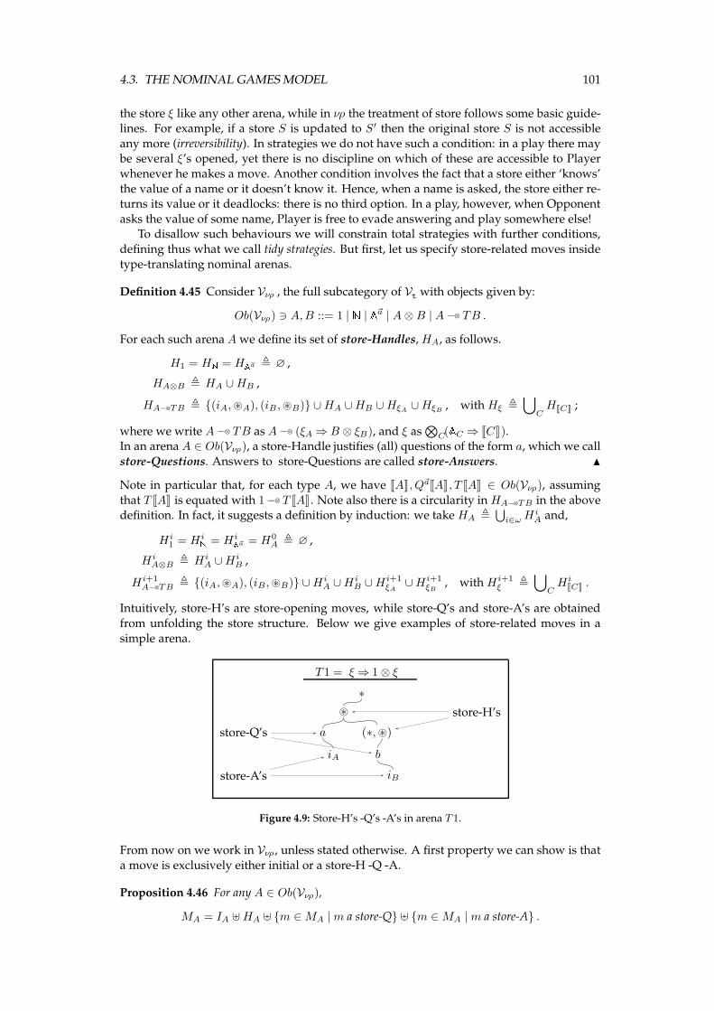
4.3. THE NOMINAL GAMESMODEL 101
the store ξ like any other arena, while in νρ the treatment of store follows some basic guide-lines. For example, if a store S is updated to S′ then the original store S is not accessible
any more (irreversibility). In strategies we do not have such a condition: in a play there maybe several ξ’s opened, yet there is no discipline on which of these are accessible to Player
whenever he makes a move. Another condition involves the fact that a store either ‘knows’
the value of a name or it doesn’t know it. Hence, when a name is asked, the store either re-turns its value or it deadlocks: there is no third option. In a play, however, when Opponent
asks the value of some name, Player is free to evade answering and play somewhere else!To disallow such behaviours we will constrain total strategies with further conditions,
defining thus what we call tidy strategies. But first, let us specify store-related moves inside
type-translating nominal arenas.
Definition 4.45 Consider Vνρ , the full subcategory of Vt with objects given by:
Ob(Vνρ) ∋ A,B ::= 1 | N | A~a | A⊗B | A −−⊗ TB .
For each such arena Awe define its set of store-Handles,HA, as follows.
H1 = HN = HA~a , ∅ ,
HA⊗B , HA ∪HB ,
HA−−⊗TB , {(iA,⊛A), (iB,⊛B)} ∪HA ∪HB ∪HξA∪HξB
, withHξ ,⋃
CHJCK ;
where we write A −−⊗ TB as A −−⊗ (ξA ⇒ B ⊗ ξB), and ξ as⊗
C(AC ⇒ JCK).In an arena A ∈ Ob(Vνρ), a store-Handle justifies (all) questions of the form a, which we call
store-Questions. Answers to store-Questions are called store-Answers. N
Note in particular that, for each type A, we have JAK, Q~aJAK, T JAK ∈ Ob(Vνρ), assuming
that T JAK is equated with 1 −−⊗ T JAK. Note also there is a circularity inHA−−⊗TB in the abovedefinition. In fact, it suggests a definition by induction: we take HA ,
⋃
i∈ωHiA and,
Hi1 = HiN = HiA~a = H0
A , ∅ ,
HiA⊗B , Hi
A ∪HiB ,
Hi+1A−−⊗TB , {(iA,⊛A), (iB,⊛B)} ∪Hi
A ∪HiB ∪Hi+1
ξA∪Hi+1
ξB, withHi+1
ξ ,⋃
CHi
JCK .
Intuitively, store-H’s are store-opening moves, while store-Q’s and store-A’s are obtained
from unfolding the store structure. Below we give examples of store-related moves in a
simple arena.
T 1 = ξ⇒ 1 ⊗ ξ
∗
⊛ store-H’s
store-Q’s a (∗,⊛)
iA b
store-A’s iB
Figure 4.9: Store-H’s -Q’s -A’s in arena T1.
From now on we work in Vνρ , unless stated otherwise. A first property we can show is that
a move is exclusively either initial or a store-H -Q -A.
Proposition 4.46 For any A ∈ Ob(Vνρ),
MA = IA ⊎HA ⊎ {m ∈MA |m a store-Q} ⊎ {m ∈MA |m a store-A} .
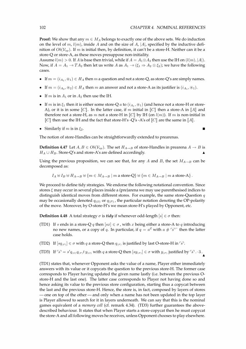
102 CHAPTER 4. NOMINAL REFERENCES
Proof: We show that anym ∈MA belongs to exactly one of the above sets. We do inductionon the level of m, l(m), inside A and on the size of A, |A|, specified by the inductive defi-
nition of Ob(Vνρ). If m is initial then, by definition, it can’t be a store-H. Neither can it be astore-Q or store-A, as these moves presuppose non-initiality.
Assume l(m) > 0. IfA is base then trivial, while ifA = A1⊗A2 then use the IH on (l(m), |A|).Now, if A = A1 −−⊗ TA2 then let us write A as A1 −−⊗ (ξ1 ⇒ A2 ⊗ ξ2); we have the followingcases.
• Ifm = (iA1 ,⊛1) ∈ HA thenm a question and not a store-Q, as store-Q’s are simply names.
• Ifm = (iA2 ,⊛2) ∈ HA thenm an answer and not a store-A as its justifier is (iA1 ,⊛1).
• Ifm is in A1 or in A2 then use the IH.
• Ifm is in ξ1 then it is either some store-Q a to (iA1 ,⊛1) (and hence not a store-H or store-
A), or it is in some JCK. In the latter case, if m initial in JCK then a store-A in JAK andtherefore not a store-H, as m not a store-H in JCK by IH (on l(m)). If m is non-initial in
JCK then use the IH and the fact that store-H’s -Q’s -A’s of JCK are the same in JAK.
• Similarly ifm is in ξ2. �
The notion of store-Handles can be straightforwardly extended to prearenas.
Definition 4.47 Let A,B ∈ Ob(Vνρ). The set HA→B of store-Handles in prearena A → B is
HA ∪HB . Store-Q’s and store-A’s are defined accordingly. N
Using the previous proposition, we can see that, for any A and B, the set MA→B can be
decomposed as:
IA ⊎ IB ⊎HA→B ⊎ {m ∈MA→B |m a store-Q} ⊎ {m ∈MA→B |m a store-A} .
We proceed to define tidy strategies. We endorse the following notational convention. Sincestores ξ may occur in several places inside a (pre)arenawe may use parenthesised indices to
distinguish identical moves from different stores. For example, the same store-Question q
may be occasionally denoted q(O) or q(P ) , the particular notation denoting the OP-polarityof the move. Moreover, by O-store-H’s we mean store-H’s played by Opponent, etc.
Definition 4.48 A total strategy σ is tidy if whenever odd-length [s] ∈ σ then:
(TD1) If s ends in a store-Q q then [sx] ∈ σ , with x being either a store-A to q introducingno new names, or a copy of q. In particular, if q = a~a with a # psq− then the latter
case holds.
(TD2) If [sq(P )] ∈ σ with q a store-Q then q(P ) is justified by last O-store-H in psq.
(TD3) If psq = s′q(O)q(P )t y(O) with q a store-Q then [sy(P )] ∈ σ with y(P ) justified by psq .−3 .N
(TD1) states that, whenever Opponent asks the value of a name, Player either immediately
answers with its value or it copycats the question to the previous store-H. The former casecorresponds to Player having updated the given name lastly (i.e. between the previous O-
store-H and the last one). The latter case corresponds to Player not having done so and
hence asking its value to the previous store configuration, starting thus a copycat betweenthe last and the previous store-H. Hence, the store is, in fact, composed by layers of stores
— one on top of the other— and only when a name has not been updated in the top layer
is Player allowed to search for it in layers underneath. We can say that this is the nominalgames equivalent of a memory cell (cf. remark 4.34). (TD3) further guarantees the above-
described behaviour. It states that when Player starts a store-copycat then he must copycatthe store-A and all following moves he receives, unless Opponent chooses to play elsewhere.
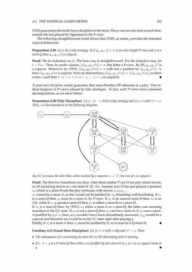
4.3. THE NOMINAL GAMESMODEL 103
(TD2) guarantees themulti-layer discipline in the store: Player can see one store at each time,namely the last played by Opponent in the P-view.
The following straightforward result shows that (TD3), as stated, provides the intendedcopycat behaviour.
Proposition 4.49 Let σ be a tidy strategy. If [s′q(O)q(P )t] ∈ σ is an even-length P-view and q is a
store-Q then q(O)q(P )t is a copycat.
Proof: We do induction on |t|. The base case is straightforward. For the inductive step, let
t = t′xz. Then, by prefix closure, [s′q(O)q(P )t′x] ∈ σ, this latter a P-view. By IH, q(O)q(P )t
′ isa copycat. Moreover, by (TD3), [s′q(O)q(P )t
′xx] ∈ σ with last x justified by (q(O)q(P )t′x).−3,
thus s′q(O)q(P )t′xx a copycat. Now, by determinacy, [s′q(O)q(P )t
′xx] = [s′q(O)q(P )t′xz], so there
exists π such that π [x = x ∧ π [x = z, ∴ x = z, as required. �
A good store discipline would guarantee that store-Handles OP-alternate in a play. This in-deed happens in P-views played by tidy strategies. In fact, such P-views have canonical
decompositions, as we show below.
Proposition 4.50 (Tidy Discipline) Let σ : AB B be a tidy strategy and [s] ∈ σ with psq = s.Then, s is decomposed as in the following diagram.
GFED@ABCiA // GFED@ABCiB //WVUTPQRSS-HOQ
�� ##**UUUUUUUUUUUUUUUUUUUUUUUUUUUUUUUU
WVUTPQRSS-HPA
��
LL
WVUTPQRSS-HPQ
��yyrrrrrrrrrrrrrrr
cc
WVUTPQRSS-QP
��WVUTPQRSS-QO
��&&LLLLLLLLLLLLLLLWVUTPQRSS-HOA
LLeeLLLLLLLLLLLLLLL
99rrrrrrrrrrrrrrr WVUTPQRSS-AO
jjUUUUUUUUUUUUUUUUUUUUUUUUUUUUUUUU
LLeeLLLLLLLLLLLLLLL
WVUTPQRSS-AP
>>
WVUTPQRSONMLHIJKCC
(by CC we mean the state that, when reached by a sequence s = psq, the rest of s is copycat.)
Proof: The first two transitions are clear. After them neither P nor O can play initial moves,
so all remaining moves in s are store-H -Q -A’s. Assume now O has just played a questionx0 which is a store-H and the play continues with moves x1x2x3... .
x1 cannot be a store-A, as this would not be justified by x0, breaching well-bracketing. If x1
is a store-Q then x2 must be a store-A, by P-view. If x1 is an answer-store-H then x2 is anOQ, while if x1 a question-store-H then x2 is either a store-Q or a store-H.
If x2 is a store-Q then, by (TD1), x3 either a store-A or a store-Q, the latter case meaning
transition to the CC state. If x2 is not a store-Q then x3 can’t be a store-A: if x3 were a store-A justified by q 6= x2 then, as q wouldn’t have been immediately answered, s≥q would be a
copycat and therefore we would be in the CC state right after playing q.Finally, if x3 is a store-A then x4 must be justified by it, so it must be a Q-store-H. �
Corollary 4.51 (Good Store Discipline) Let [s] ∈ σ with σ tidy and psq = s. Then:
• The subsequence of s containing its store-H’s is OP-alternating and O-starting.
• If s.−1 = q is a P-store-Q then either q is justified by last store-H in s, or s is in copycat mode at
q. �
104 CHAPTER 4. NOMINAL REFERENCES
Our next aim is to show that νρ is modelled inside the subcategory of Vνρ with tidy strate-
gies. We first need to show that tidy strategies indeed form a subcategory of Vνρ , and thenthat all the structure necessary for the νρ-model is available in tidy strategies. The following
proposition gives equivalent definitions of tidy strategies, which will be of use in the sequel.
Proposition 4.52 Let σ be a strategy.
1. σ is tidy iff whenever odd-length [s] ∈ σ then (TD1,2,3′) hold, where:
(TD3′) If psq = s′q(O)q(P )t y(O) with q a store-Q and q(O)q(P )t a copycat then [sy(P )] ∈ σ
with y(P) justified by psq .−3.
2. (a) σ is tidy iff whenever odd-length [s] ∈ σ with psq = s then (TD1,2,3) hold,
(b) σ is tidy iff whenever odd-length [s] ∈ σ with psq = s then (TD1,2,3′) hold.
Proof: For 1, it suffices to show that whenever σ satisfies (TD1,2,3′) and [s′q(O)q(P )t y] ∈ σ is
a P-view and q a store-Q, then q(O)q(P )t is a copycat. But this is shown exactly as proposi-
tion 4.49, replacing “by (TD3)” by “by (TD3′)”.For 2, we show only the first part, the other part is shown similarly. We need only show the
“if” direction. So assume the RHS hypothesis and let odd-length [s] ∈ σ, so [psq] ∈ σ.If s ends in a store-Q q, then so does psq, so [psqx] ∈ σ, with x being a store-A not introducing
new names or a copy of q. But x non-introducing and [s], [psq x] ∈ σ implies [sx] ∈ σ, by
lemma 3.38. If, in particular, q = a with a# psq− then x is a copy of q.If [sq] ∈ σ with q a store-Q then [psq q] ∈ σ so q justified by last O-store-H in psq.If psq = s′q(O)q(P )ty with q a store-Q then [psq y] ∈ σ with last y justified by psq .−3. Bylemma 3.38, [sy] ∈ σ, as required. �
We can now show that strategies which ‘mostly do copycats’ are tidy.
Corollary 4.53 A strategy σ is tidy if, for any odd-length [s] ∈ σ with psq = s and |s| ≥ 5:
1. If ∀x. [sx] /∈ σ then s.−1 is not a store-Q and there are no consecutive store-Q’s q(O)q(P ) inside s.
2. If [sx] ∈ σ and x 6= s.−1 then s doesn’t contain any q(O)q(P ) and also:
(a) if s.−1 a store-Q then x is an answer to s.−1 not introducing new names and s.−1 = a~a with
a ∈ S(s−),
(b) if x a store-Q then it is justified by last O-store-H in s.
3. If [sx] ∈ σ and x = s.−1 then one of the following is the case:
(a) s doesn’t contain any q(O)q(P ), and if x a store-Q then justified by last O-store-H in s;
(b) x is justified by s.−3.
Proof: By proposition 4.52, it suffices to show that such an s satisfies (TD1,2,3). For (TD1),
if s.−1 a store-Q then |s| ≥ 5 and, by 1, [sx] ∈ σ, for some x. If x is not a copy of s.−1 then,by 2a, s.−1 is not a fresh name and x is a non-intro answer to s.−1, as required. For (TD3), if
s = s′q(O)q(P )t y(O) then |s| ≥ 7 and, by 1,2, [sy] ∈ σ and, by 3, y is justified by s.−3. Finally,
for (TD2), if [sx] ∈ σ with x a store-Q then |s| ≥ 3. If |s| = 3 then x necessarily justifiedby s.−1 and that is the last O-store-H in s, as s.1, s.2 are initial moves. If |s| ≥ 5 then either
cases 2b,3a apply, or x = s.−1 and x justified by s.−3. In the latter case, s.−1 is an O-store-Q
justified by s.−2, hence s.−3 is the last O-store-H in s, as required. �
Thus, for example, identity arrows are tidy as they fall under case 3b. In fact, as we willshow later, all important structure is tidy. Let us now proceed to closure of tidy strategies
under composition.
4.3. THE NOMINAL GAMESMODEL 105
Lemma 4.54 Let σ : AB B and τ : BB C be tidy strategies, and let [s ; t] ∈ σ ; τ , [s] ∈ σ and[t] ∈ τ , with ps ‖ tq = s ‖ t ending in a generalised O-move in AB and x, an O-move, being the last
store-H in psq. Let x appear in s ‖ t as x. Then, x is the last store-H in s ‖ t and if x is in A then allmoves after x in s ‖ t are in A. Similarly for BC and t.
Proof: We show the (AB, s) case, the other case being entirely dual. Let s = s1xs2 and let
x appear in s ‖ t as some x. If x is in A then we claim that s2 is in A. Suppose otherwise,
so s = s1xs21ys22 with s21 in A and y a P-move in B. Since x appears in psq, the wholeof s21y appears in it, as it is in P-view mode already. Since x is last store-H in psq, s21y is
store-H-less. If y a store-Q then it should be justified by last O-store-H in ps<yq, that is x,which is not possible as x is in A. Thus, y must be a store-A, say to some O-store-Q q in B.
Now, since q wasn’t immediately answered by P, tidiness dictates that psq be a copycat from
move q and on. But then the move following x in s must be a copy of x in B, . Hence, s2is in A and therefore it appears in psq, which implies that it is store-H-less. Thus, x is last
store-H in s ‖ t.If x is in B then we do induction on |s ‖ t|. The base case is encompassed in the case of s2being empty, which is trivial. So let s2 = s21ys22z with y justifying z (since x appears in psq,z has to be justified in s2). z is not a store-H and neither is it a store-Q, as then y would be astore-H after x in psq. Thus z a store-A and y a store-Q, the latter justified by last O-store-H in
ps<yq = psq<y , that is x, so y, z in B. Now, s = s1xs21ys22z and t = t1x′t21y
′t22z′ ; we claim
that s21 and t21 are store-H-less. Indeed, s<y ‖ t<y′ ends in a generalised O-move in AB and
x is still the last store-H in ps<yq , from which we have, by IH, that x is the last store-H in
s<y ‖ t<y′ .Thus, s ‖ t = (s1 ‖ t1)xvyuz with v store-H-less. It suffices to show that u is also store-H-
less. In fact, u = y . . . y︸ ︷︷ ︸
n
z . . . z︸ ︷︷ ︸
n
for some n ≥ 0. Indeed, by tidiness of τ , (t22z′).1 is either
an answer to y′, whence t22 = u = ǫ, or a copy of it under the last O-store-H in pt≤y′q. Ifthe latter is in B then σ reacts analogously, and so on, so there is initially a sequence y . . . y
in u, played in B. As u finite, at some point σ (or τ ) either answers y (y′) or copycats it inA (in C). In the latter case, O immediately answers, as s (t) is in P-view mode in A (in C).
Hence, in either cases there is an answer that is copycatted to all open y in u, yielding thus
the required pattern. Therefore, u is store-H-less. �
Lemma 4.55 Let σ : A B B and τ : B B C be tidy strategies, and let [s ; t] ∈ σ ; τ , [s] ∈ σ
and [t] ∈ τ , with ps ‖ tq = s ‖ t ending in a generalised O-move. If there exists i ≥ 1 and store-Q’sq1, ..., qi with q = qj , all 1 ≤ j ≤ i, and q1, ..., qi−1 in B and qi in AC and [(s ‖ t)q1...qi] ∈ σ ‖ τ ,then qi is justified by the last O-store-H in s ; t.
Proof: By induction on |s ‖ t|. The base case is encompassed in the case of s ; t containingat most one O-store-H, which is trivial. Now let wlog (s ‖ t)q1...qi = (sq1...qi) ‖(tq′1...q
′i−1)
with [sq1...qi] ∈ σ and [tq′1...q′i−1] ∈ τ , and let each qj be justified by xj and each q′j by x
′j .
Moreover, by hypothesis, xj = x′j , for 1 ≤ j ≤ i − 1, and therefore each such pair xj , x′j
appears in s ‖ t as some xj , the latter justifying qj in s ‖ t.Now, assume wlog that s ‖ t ends in AB. Then, by tidiness of σ and τ we have that, for each
j ≥ 1,
q2j+1 = q2j , q′2j = q′2j−1 , qj = q′j
For each j ≥ 1, q2j+1 is a P-move of σ justified by some store-H, say x2j+1. By tidiness ofσ, x2j+1 is the last O-store-H in ps<q2j+1q = ps≤q2j
q, and therefore x2j+1 is the last store-H
in ps<x2jq. Then, by previous lemma, x2j+1 is the last store-H in s<x2j
‖ t<x′2j
= (s ‖ t)<x2j.
Similarly, x2j is the last store-H in (s ‖ t)<x2j−1 . Hence, the store-H subsequence of (s ‖ t)≤x1
ends in xi...x1.
Now, by tidiness of σ, x1 is the last O-store-H in psq. If x1 is also the last store-H in psq then, byprevious lemma, x1 is the last store-H in s ‖ t, hence xi is the last store-H in s ; t. Otherwise,
by corollary 4.51, q1 is a copy of s.−1 = q0 . If q0 is in A then its justifier is s.−2 = x0 and,
106 CHAPTER 4. NOMINAL REFERENCES
because of CC-mode, the store-H subsequence of s ‖ t ends in xi...x1x0 , so xi is the last O-store-H in s ; t. If q0 is in B then we can use the IH on s− ‖ t− and q0, q1, ..., qi, and obtain
that xi is the last O-store-H in s− ; t− = s ; t. �
Proposition 4.56 If σ : AB B and τ : BB C are tidy strategies then so is σ ; τ .
Proof: Take odd-length [s ; t] ∈ σ ; τ with not both s and t ending in B, ps ‖ tq = s ‖ t and|s ; t| odd. We need to show that s ; t satisfies (TD1-3). As (TD2) is a direct consequence ofthe previous lemma, we nos the other two conditions. Assume wlog that s ; t ends in A.
For (TD1), assume s ; t ends in a store-Q q. Then s ends in some q, which is justified by the
P-store-H s.−2 = x (also in A). q is either answered or copied by σ ; in particular, if q = a~a
with a # ps ; tq− = s− ; t then a # s−, t , so σ copies q. If σ answers q with z then z doesn’t
introduce new names, so [(s ; t)z] ∈ σ ; τ with nlist(z) = nlist(q) and z = z , as required.Otherwise, let σ copy q as q1 , say, under last O-store-H in psq, say x1. If x1 is in B then, by
lemma 3.41, sq1 ≍ tq′1, with q1, q′1 in B and q′1 being q1 with name-list that of its justifier, say
x′1, where x1 = x′1 . Now [tq′1] ∈ τ and it ends in a store-Q, so τ either answers it or copies
it under last O-store-H in ptq′1q. In particular, if q = a~a with a # ps ; tq then, as above, a # t
and τ copies q′1. This same reasoning can be applied consecutively, with copycats attachingstore-Q’s to store-H’s appearing each time earlier in s and t. As the latter are finite and
initial store-H’s are third moves in s and t, at some point either σ plays qi in A or answers it
in B, or τ plays q′i in C or answers it in B. If an answer occurs then it doesn’t introduce newnames (by tidiness), so it is copycatted back to q closing all open qj ’s and q
′j ’s. Otherwise,
we need only show that, for each j, qj = q, which we do by induction on j: q1 = qs • t,ǫ and
qj+1 = q(s≤qj
) •(t≤q′j),ǫ
= qjIH= q. This proves (TD1).
For (TD3), assume s ; t = uq(O)q(P )vy with q(O)q(P )v a copycat. Then, either both q(O), q(P )
are in A, or one is in A and the other in C. Let’s assume q(O) in A and q(P ) in C— the
other cases are shown similarly. Then, q(O) her(editarily)-justifies y, and let s.−1 = y be
justified by some x in s. Now, as above, q(O)q(P ) is witnessed by some q(O) q1 . . . qiq(P ) ins ‖ t, with odd i ≥ 1 and all qj ’s in B. We show by induction on 1 ≤ k ≤ i that there exist
x1, ..., xk, x′1, ..., x
′k, y1, ..., yk, y
′1, ..., y
′k in B such that (sy1 . . . yk ‖ ty′1 . . . y
′k) ∈ σ ‖ τ and, for
each relevant j ≥ 1,
yj = y′j = y , y1 = y , y2j = y2j+1 , y′2j−1 = y′2j , xj = x′j
with qj her-justifying xj in s and xj justifying yj (and q′j her-justifying x
′j in t and x
′j justify-
ing y′j), and xj+1, xj consecutive in s ‖ t, and x1, x also consecutive.
For k = 1, let s = s1q(O)q1s2y. Now, q(O) her-justifying y implies that q(O) her-justifies
y, hence it appears in psq. Thus psq = s′1q(O)q1s′2y, so, by (original definition of) tidiness,
[sy1] ∈ σ with y1 = y justified by x1 = psq .−3 = s.−3. By lemma 3.41, [ty′1] ∈ τ with y′1 = y1.
By proposition 4.49, q(O)q1s′2 is a copycat, so q1 her-justifies x1 and therefore x1, y1 in B. Fi-
nally, x = psq .−2 = s.−2 is a P-move so x1, x are consecutive in s ‖ t.For even k > 1 we have, by IH, that (sy1 . . . yk−1 ‖ ty′1 . . . y
′k−1) ∈ σ ‖ τ with y′k−1 an O-
move her-justified by q′k−1, an O-move. Then, q′k−1 appears in pty′1...y′k−1q, so pty′1...y
′k−1q =
t1q′k−1q
′kt2y
′k−1, thus (by tidiness) [ty
′1...y
′k−1y
′k] ∈ τ with y′k = y′k−1 justified by x′k = pty′1...y
′k−1q .−3.
Now, q′k−1q′kt2 is a copycat so q′k her-justifies x′k. Moreover, x′k, x
′k−1 are consecutive in ptq,
so, as x′k−1 a P-move, they are consecutive in t, and therefore xk, xk−1 consecutive in s ‖ t.Finally, by lemma 3.41, [sy1 . . . yk−1yk] ∈ σ with yk = y′k. The case of k odd is entirely dual.
Now, working as above, we can show that there exist x′i+1, y′i+1 inC such that [ty′1...y
′iy
′i+1] ∈
τ and y′i+1 justified by x′i+1, x′i+1 her. justified by q(P ), etc. Then [(s ; t)yi+1] ∈ σ ; τ with
xi+1, xi, ..., x1, x consecutive in s ‖ t, so xi+1 = (s ; t).−3. Finally, as above, yi+1 = yj = y, all
j, as required. �
Hence, we can define our category of nominal arenas and tidy strategies.
Definition 4.57 T is the lluf subcategory of Vνρ of tidy strategies. N
4.3. THE NOMINAL GAMESMODEL 107
We now check that all structure required for a sound νρ-model pass from Vt to T .
Proposition 4.58 (T an adequate model) T forms an adequate νρ-model by inheriting the nec-essary structure from Vt:
I. Projections and terminal arrows are tidy, and arrow pairing preserves tidiness.
II. ηA, τA, µA are tidy, and if h is tidy then so is Th. Moreover, ΛT preserves and reflects tidiness.
III. Successor, predecessor, numeral and conditional arrows are tidy.
IV. εA, δA, ζA are tidy, and if h is tidy then so is Q~ah, for any ~a. Moreover,(~a~a′
)
Aand nuA are
tidy.
V. Name-equality arrows are tidy.
VI. updA, drfA are tidy.
Proof: Items III and V involve strategies with plays of length less than 3, hence tidy. The
same holds for terminal arrows in I and(~a~a′
)
1in IV. From corollary 4.53 we have that pro-
jections in I; ηA, τA, µA in III; nuA in IV; and updA, drfA in VI are all tidy.
Now let f : A→ B, g : A→ C be tidy strategies. Then,
viewf(〈f, g〉) = { [iA (iB, iC) s] | ([iA iB s] ∈ viewf(f) ∧ [iA iC ] ∈ g)
∨ ([iA iC s] ∈ viewf(g) ∧ [iA iB ] ∈ f) }
So let odd-length [s] ∈ 〈f, g〉 with psq = s and |s| ≥ 5, say wlog s = iA (iB, iC) s′ x with[iA iB s
′] ∈ viewf(f) and [iA iC ] ∈ g. It is not difficult to see then that [sf ] ∈ f , for sf =
iA iB s′ x. If x is a store-Q then [sf y] ∈ viewf(f) for a relevant y, and so [s y] ∈ viewf(〈f, g〉).
We need only check the case of x = a~a with a # s−, which implies a # s−f and hence y acopy of x, as required. Now, if [s y] ∈ viewf(〈f, g〉) with y a store-Q then [sf y] ∈ viewf(f),
so y is justified by last O-store-H in sf , and hence y justified by last O-store-H in s. Fi-nally, if s = iA (iB, iC) s′′q(O) q(P ) t x(O) then sf = s = iA iB s
′′q(O) q(P ) t x(P ), and therefore
[sf x] ∈ viewf(f) with x(P ) justified by sf .−3 and [s x(P )] ∈ viewf(〈f, g〉), as required. Hence,
〈f, g〉 tidy.In along the same lines we can prove that T preserves tidiness, and that ΛT preserves and
reflects tidiness. Moreover, tidiness of product-related constructs implies tidiness of struc-tural arrows in the comonads.
Finally, adequacy is clearly inherited from Vt. �
Henceforth, by strategies we shall mean tidy strategies, unless stated otherwise.
4.3.6 Observationality
Strategy equality is too fine grained to capture contextual equivalence in a complete manner.For example, even simple contextual equivalences like
skip ≅ νa.skip
are not preserved by the semantical translation, since strategies include in their name-listsall introduced names, even useless ones. For similar reasons, equivalences like
νa.νb.M ≅ νb.νa.M
are not valid semantically. It is not only because of the treatment of name-creation thatthe semantics is not complete. The ‘explicit’ way in which the store works distinguishes
equivalences likea := 1 ;λx. ! a ; 2 ≅ a := 1 ;λx.2 .
108 CHAPTER 4. NOMINAL REFERENCES
Thus, there are many ways in which our semantics is too expressive for our language. Wetherefore proceed to apply a quotienting by the intrinsic preorder and prove full-abstraction
in the extensional model.Following the steps described in section 4.2.2, in this section we introduce the intrinsic
preorder on T and show that the resulting model is observational. Full-abstraction is then
shown in the following section.
Definition 4.59 Expand T to (T , T,Q,O) by setting, for each ~a ∈ A#,
O~a , {f ∈ T (Q~a1, TN) | ∃~b. [(~a, ∗) ∗ ⊛ (0,⊛)~b] ∈ f} .
Then, for each f, g ∈ T (Q~aA, TB), f .~a g if
∀ρ : Q~a(A −−⊗ TB)B TN. (Λ~a(f) ; ρ ∈ O~a =⇒ Λ~a(g) ; ρ ∈ O~a) .N
Thus, the observability predicate O is a family (O~a)~a∈A# , and the intrinsic preorder . is a
family (.~a)~a∈A# . Recall that by Λ~a(f) we mean ΛQ~a,T (f), that is,
Λ~a(f) = Q~a1 δPA Q~aQ~a1Q~aΛ(z ′ ; f)PPPPPPPPA Q~a(A −−⊗ TB) .
In particular, if f ⊑ g then Λ~a(f) ⊑ Λ~a(g) and therefore Λ~a(f) ; ρ ⊑ Λ~a(g) ; ρ, which implies:
f ⊑ g =⇒ f .~a g (4.16)
The intrinsic preorder is defined by use of test arrows ρ, which stand for possible programcontexts. As the following result shows, not all such tests are necessary.
Lemma 4.60 (tl4 tests suffice) Let f, g ∈ T (Q~a1, B) with B pointed. The following are equiva-
lent.5
I. ∀ρ : Q~aBB TN. δ ;Q~af ; ρ ∈ O~a =⇒ δ ;Q~ag ; ρ ∈ O~a .
II. ∀ρ : Q~aBB TN. ρ is tl4 =⇒ (δ ;Q~af ; ρ ∈ O~a =⇒ δ ;Q~ag ; ρ ∈ O~a) .
Hence, for each ~a and f, g ∈ T (Q~aA, TB), f .~a g iff
∀ρ : Q~a(A −−⊗ TB)B TN. ρ is tl4 =⇒ (Λ~a(f) ; ρ ∈ O~a =⇒ Λ~a(g) ; ρ ∈ O~a) .
Proof: I ⇒ II is trivial. Now assume II holds and let ρ : Q~aB B TN be any strategy
such that δ ;Q~af ; ρ ∈ O~a. Then, there exist [s] ∈ δ ;Q~af and [t] ∈ ρ such that [s ; t] =
[(~a, ∗) ∗ ⊛ (0,⊛)~b] ∈ (δ ;Q~af) ; ρ. We show by induction on the number of JB-moves ap-
pearing in s ‖ t that δ ;Q~ag ; ρ ∈ O~a.
If no suchmoves appear then t = (~a, iB) ∗⊛ (0,⊛)~b, so done. If n+1 suchmoves appear then
ρ is necessarily t4, asB is pointed, so by lemma 3.58 there exists tl4* strategy ρ such that ρ =
∆ ; ρ. It is not difficult to see that ρ being tidy implies that ρ is tidy. Moreover, δ ;Q~af ; ρ =
δ ;Q~af ; ∆ ; ρ = δ ;Q~af ;〈id, Q~a! ; δ ;Q~af〉 ; ρ = δ ;Q~af ; ρ′ , with ρ′ being 〈id, Q~a! ; δ ;Q~af〉 ; ρ.
Now, by definition of ρ, [(~a, ∗) ∗ ⊛ (0,⊛)~b] = [s′ ; t′] ∈ δ ;Q~af ; ρ′ with s′ ‖ t′ containing
n JB-moves so, by IH, δ ;Q~ag ; ρ′ ∈ O~a. But δ ;Q~ag ; ρ′ = δ ;Q~ag ;〈id, Q~a! ; δ ;Q~af〉 ; ρ =
δ ;Q~af ;〈Q~a! ; δ ;Q~ag, id〉 ; ρ = δ ;Q~af ; ρ′′ , with ρ′′ being 〈Q~a! ; δ ;Q~ag, id〉 ; ρ. But ρ′′ is tl4,thus, by hypothesis, O~a ∋ δ ;Q~ag ; ρ′′ = δ ;Q~ag ; ρ , as required. �
We can now prove the second half of observationality.
5Recall, from definition 3.51, that a total strategy σ : A −→ B is:
• l4 if whenever [s] ∈ σ and s.−1 ∈ JA then |psq | = 4,
• t4 if for any [iA iB jB ] ∈ σ there exists [iA iB jB j~bA] ∈ σ,
• tl4 if it is both t4 and l4,
• ttotal if it is tl4 and for any [iA iB jB ] ∈ σ there exists [iA iB jB jA] ∈ σ.
4.3. THE NOMINAL GAMESMODEL 109
Lemma 4.61 For any f : Q~a′
1B B and any tl4 morphism ρ : Q~aBB TN, with B pointed and~a ⊆ ~a′,
δ ;Q~a \~a^~a′℄ f ; ρ ∈ O~a ⇐⇒ δ ;Q~a′
f ; ~a′
~a ; ρ ∈ O~a′
.
Moreover, for all relevant f, g and ~a ⊆ ~a′′ ⊆ ~a′,
f .~a′ g =⇒ \~a^~a′℄ f .~a \~a^~a′℄ g ,f .~a g =⇒ ~a′
~a ; f .~a′ ~a′
~a ; g ,
~a′
~a′′ ; f .~a′ g =⇒ \~a^~a′′℄ f .~a \~a^~a′℄ g .In particular, f .~aa g =⇒ \a℄ f .~a \a℄ g .Proof: For the first part, ρ being tl4 and B being pointed imply that there exists some ~b# ~a
and a ttotal strategy ρ′ such that ρ = \~b℄ ρ′. Now let δ ;Q~a \~a^~a′℄ f ; ρ ∈ O~a, so there exists
[s ; t] = [(~a, ∗) ∗ ⊛ (0,⊛)~b(~a′\~a)~c] ∈ (δ ;Q~a \~a^~a′℄ f) ; ρ, and let s = (~a, ∗) (~a, iB) jBm
(~a′\~a)~cs′
and t = (~a, iB) ∗⊛ j~bB t
′. Letting s′rα be s′nlist(s′)\(~a′\~a)
, we can see that [(~a′, ∗) iB jBm~cs′rα] ∈
f and thus [s′′] , [(~a′, ∗) (~a, iB) jBm~cs′rα] ∈ δ ;Q~a
′
f ; ~a′
~a . Hence, [s′′ ; t] = [(~a′, ∗) ∗⊛ (0,⊛)~b~c] ∈
δ ;Q~a′
f ; ~a′
~a ; ρ, as required. The converse is shown similarly.
For the second part, suppose f .~a′ g : Q~a′
A B TB and take any tl4 morphism ρ :
Q~a(A −−⊗ TB)B TN. Then,Λ~a(\~a^~a′℄ f) ; ρ ∈ O~a ⇐⇒ δ ;Q~aΛ(ζ ′ ; \~a^~a′℄ f) ; ρ ∈ O~a
(3.12)⇐⇒ δ ;Q~a \~a^~a′℄(Λ(ζ ′ ; f)) ; ρ ∈ O~a
⇐⇒ δ ;Q~a′
Λ(ζ ′ ; f) ; ~a′
~a ; ρ ∈ O~a′
f.~a′g
=⇒ δ ;Q~a′
Λ(ζ ′ ; g) ; ~a′
~a ; ρ ∈ O~a′
⇐⇒ Λ~a(\~a^~a′℄ g) ; ρ ∈ O~a.
For the next claim, it is easy to see that, for any h : Q~a′
1B TN, h ∈ O~a′
iff(~a~a′
);h⊥ ; pu ∈ O~a.
Hence, if f .~a g then we have:
δ ;Q~a′
Λ(ζ ′ ; ~a′
~a ; f) ; ρ ∈ O~a′
⇐⇒ δ ;Q~a′ ~a′
~a ;Q~a′
Λ(ζ ′ ; f) ; ρ ∈ O~a′
⇐⇒(~a~a′
);(δ ;Q~a
′ ~a′
~a ;Q~a′
Λ(ζ ′ ; f) ; ρ)⊥ ; pu ∈ O~a
(N2’)⇐⇒ δ ;Q~aΛ(ζ ′ ; f) ;
(~a~a′
); ρ⊥ ; pu ∈ O~a
f.~ag=⇒ δ ;Q~aΛ(ζ ′ ; g) ;
(~a~a′
); ρ⊥ ; pu ∈ O~a ⇐⇒ δ ;Q~a
′
Λ(ζ ′ ; ~a′
~a ; g) ; ρ ∈ O~a′
.
For the last claim, if ~a′
~a′′ ; f .~a′ g then \~a^~a′℄( ~a′~a′′ ; f) .~a \~a^~a′℄ g, so it suffices to show\~a^~a′℄( ~a′~a′′ ; f) ⋍ \~a^~a′′℄ f . Now, observing that, for any h : Q~a′′
1 B TN, h ∈ O~a′′
iff~a′
~a′′ ;h ∈ O~a′
, we have:
δ ;Q~aΛ(ζ ′ ; \~a^~a′℄( ~a′~a′′ ; f)) ; ρ ∈ O~a(3.12)⇐⇒ δ ;Q~a \~a^~a′℄Λ(ζ ′ ; ~a
′
~a′′ ; f) ; ρ ∈ O~a
⇐⇒ δ ;Q~a′
Λ(ζ ′ ; ~a′
~a′′ ; f) ; ~a′
~a ; ρ ∈ O~a′
⇐⇒ ~a′
~a′′ ; δ ;Q~a′′
Λ(ζ ′ ; f) ; ~a′′
~a ; ρ ∈ O~a′
⇐⇒ δ ;Q~a′′
Λ(ζ ′ ; f) ; ~a′′
~a ; ρ ∈ O~a′′
⇐⇒ δ ;Q~a \~a^~a′′℄Λ(ζ ′ ; f) ; ρ ∈ O~a(3.12)⇐⇒ δ ;Q~aΛ(ζ ′ ; \~a^~a′′℄ f) ; ρ ∈ O~a,
as required. �
In order to prove that T is observational, we are only left to show that
JMK ∈ O~a ⇐⇒ ∃~b, S. JMK = \~b℄ JS ; 0K
for any ~a ^∅_M : N. The “⇐=” direction is trivial. For the converse, because of correct-ness, it suffices to show the following generalisation of adequacy.6
6At this point, notice that the proof of adequacy (proposition 4.44) is, in fact, a proof of O-adequacy. As we findboth proofs interesting, we present them both regardless of the redundancy.
110 CHAPTER 4. NOMINAL REFERENCES
Lemma 4.62 (O-Adequacy) Let ~a ^∅_M : N be a typed term. If JMK ∈ Oǫ then there existssome S such that ~a`M −→→ S ` 0.
Proof: The idea behind the proof is the same as that of the proof of adequacy (v. sec-tion 4.3.4). It suffices to show that, for any suchM , there is a non-reducing sequent S ` N
such that ~a ` M −→→ S ` N ; therefore, because of Strong Normalisation in the sν-calculus, it suffices to show that there is no infinite reduction sequence starting from ~a`M
and containing infinitely many DRF reduction steps.
To show the latter we will use an operation on terms adding new-name constructors justbefore dereferencings. The operation yields, for each termM , a term (M)[ the semantics of
which is equivalent to that of M . On the other hand, ~a ` (M)[ cannot perform infinitelymany DRF reduction steps without creating infinitely many new names. For each termM ,
define (M)[by induction as:
(a)[ , a , (x)[ , x , ... (λx.M)[ , λx.(M)[ , (M N)[ , (M)[(N)[ , ...
and (!N)[ , νa. !(N)[ , some a /∈ fn(N).
We show that J(M)[K ⋍ JMK, by induction on M ; the base cases are trivial. The inductionstep follows immediately from the IH and the fact that ⋍ is a congruence, in all cases except
for M being !N . In the latter case we have that J(M)[K = \a℄(~aa~a ; J!(N)[K) , while the IHimplies that JMK ⋍ J!(N)[K. Hence, it sts that for each f : Q~aA B TB we have f ⋍\a℄(~aa~a ; f) . Indeed, for any relevant ρ which is tl4,
Λ~a(\a℄(~aa~a ; f)) ; ρ ∈ O~alem 4.61⇐⇒ δ ;Q~aaΛ(ζ ′ ; ~aa~a ; f) ; ~aa~a ; ρ ∈ O~aa
⇐⇒ δ ;Q~aa~aa~a ; ~aa~a ;Q~aΛ(ζ ′ ; f) ; ρ ∈ O~aa
⇐⇒ ~aa~a ; Λ~a(f) ; ρ ∈ O~aa ⇐⇒ Λ~a(f) ; ρ ∈ O~a .
Now, take any ~a ^∅_M : N and assume JMK ∈ O~a, and that ~a ` M diverges us-
ing infinitely many DRF reduction steps. Then, ~a ` (M)[ diverges using infinitely manyNEW reduction steps. However, since J(M)[K ⋍ JMK, we have J(M)[K ∈ O~a and therefore
[(~a, ∗) ∗ ⊛ (0,⊛)~b] ∈ J(M)[K for some ~b. However, ~a ` (M)[ reduces to some S ` M ′ us-
ing |~b|+1NEW reduction steps, so J(M)[K = \~c℄ JS ;M ′K with |~c| = |~b|+1,to determinacy.�
We have therefore shown observationality.
Proposition 4.63 (Observationality) (T , T,Q,O) is observational. �
4.3.7 Definability and full-abstraction
We now proceed to show definability in our model T , and through it ip-definability. Ac-
cording to the results of section 4.2.2, this will suffice for full abstraction.
We first make precise the notion of finitary strategy, that is, of strategy with finite descrip-tion, by introducing truncation functions that remove inessential branches from a strategy’s
description.
Definition 4.64 Let σ : A B B in T and let [s] ∈ viewf(σ) be of even length. Definetrunc(s) and trunc′(s) by induction as follows.
trunc(ǫ) = trunc′(ǫ) , ǫ
trunc(x(O)y(P )s′) ,
{
ǫ , if x = y are store-Q’s
xy trunc(s′) , o.w.
trunc′(x(O)y(P )s′) ,
ǫ , if x = y are store-Q’s
ǫ , if x store-Q , y a store-A and s′ = ǫ
ǫ , if x ∈ IA, y ∈ IB and s′ = ǫ
xy trunc′(s′) , o.w.
4.3. THE NOMINAL GAMESMODEL 111
Moreover, say σ is finitary if trunc(σ) is finite, where
trunc(σ) , {[trunc(s)] | [s] ∈ viewf(σ) ∧ |s| > 3} .
Finally, for any [t] ∈ σ define:
σ≤t , strat{[s] ∈ viewf(σ) | ∃ t′ ≤ t. trunc′(s) = pt′q} .N
Hence, finitary are those strategies whose viewfunctions become finite if we delete all thestore-copycats and all default initial answers— the latter dictated by totality. Moreover,
the strategy σ≤t is the strategy we are left with if we truncate viewf(σ) by removing all its
branches of size greater than 3 that are not contained in t, except for the store-copycatswhichare left intact and for the store-A’s brancheswhich are truncated to the point of leaving solely
the store-A, so that we retain tidiness.Note that, in general, trunc′(s) ≤ trunc(s) ≤ s. We can then show the following.
Proposition 4.65 If σ is a strategy and [t] ∈ σ is even-length then σ≤t is a finitary strategy with
[t] ∈ σ≤t and σ≤t ⊑ σ.
Proof: To show that σ≤t is an innocent strategy we need to show that
f , {[s] ∈ viewf(σ) | ∃ t′ ≤ t. trunc′(s) = pt′q}
is a viewfunction. For even-prefix closure, if s = s′xy and [s] ∈ f then [s] ∈ viewf(σ) and
trunc′(s) = pt′q, some t′ ≤ t. We have that trunc′(s′) ≤ trunc′(s) so trunc′(s′) = pt′′q, somet′′ ≤ t′ ≤ t, so [s′] ∈ f . Single-valuedness is clear, as f ⊆ viewf(σ). The latter shows also
that σ≤t ⊑ σ.
Totality is obvious. For tidiness, let odd-length [s] ∈ σ≤t with psq = s. (TD2) clearlyholds. For (TD1), if s ends in a store-Q then there exists [sx] ∈ σ satisfying (TD1) and,
as trunc′(s−) = trunc′(sx), we have [sx] ∈ f . The same reasoning resolves (TD3).We now show trunc(f) is finite. Each [s′] ∈ trunc(f) is [trunc(s)] for some [s] ∈ viewf(σ)
and t′ ≤ t such that |s| > 3 and trunc′(s) = pt′q. The cases of [trunc(s)] = [trunc′(s)] are
finitely many, as t is of finite length. For the rest, trunc(s) = trunc′(s)xy , x a store-Q awitha ∈ S(trunc′(s)) and y a store-A. Hence, for each t′ ≤ t there are not more than |S(pt′q)|-many elements added in trunc(f). Thus, σ≤t is finitary.Finally, for any even-length t′ ≤ t, we have that trunc′(pt′q) ≤ pt′q, so there exists some t′′ ≤ t
such that trunc′(pt′q) = pt′′q and hence [pt′q] ∈ σ≤t. Then, by lemma 3.38, we have [t] ∈ σ≤t.�
We proceed to show definability. The proof is facilitated by the following lemma. Note
that for economy we define strategies by means of their viewfunctions modulo totality andeven-prefix closure. Moreover, we write σ ↾ i for the (total) restriction of a strategy σ to an
initial move i, and sr~b for swith~b removed from all of its name-lists.
Lemma 4.66 (Decomposition Lemma) Let σ : Q~aJAK B T JBK be a strategy. We can decom-
pose σ as follows.
1. If there exists an iA(0) such that ∃x0. [(~a, iA(0)) ∗ ⊛ x0] ∈ σ then
σ = Q~aJAK〈[x
~a= iA(0)], 〈σ0, σ
′〉〉PPPPPPPPPPPPPPPA N⊗ (T JBK)2cndPPA T JBK
where:
[x~a= iA(0)] : Q~aJAK B N , {[(~a, iA(0)) 0]} ∪ {[(~a, iA) 1] | [(~a, iA)] 6= [(~a, iA(0))]} ,
σ0 : Q~aJAK B T JBK , strat{ [(~a, iA(0)) s] ∈ viewf(σ) } ,
σ′ : Q~aJAK B T JBK , strat{ [(~a, iA) s] ∈ viewf(σ) | [(~a, iA)] 6= [(~a, iA(0))] } .

112 CHAPTER 4. NOMINAL REFERENCES
2. If there exists an iA(0) such that ∀iA. (∃x0. [(~a, iA) ∗ ⊛ x0] ∈ σ) ⇐⇒ [(~a, iA)] = [(~a, iA(0))] ,
then σ = \~b℄σ~b , where:σ~b : Q~a
~bJAK B T JBK , strat{ [(~a~b, iA(0))∗⊛m0 sr~b] | [(~a, iA(0)) ∗⊛m
~b0 s] ∈ viewf(σ) } .
3. If there exist iA(0),m0 such that ∀iA, x. [(~a, iA) ∗ ⊛ x] ∈ σ ⇐⇒ [(~a, iA)x] = [(~a, iA(0))m0] ,then one of the following is the case.
(a) m0 = a, a store-Q of type C under ⊛, in which case we have σ = σ′ ↾ (~a, iA(0)), where:
σ′ , Q~aJAK〈id, φ〉PPPPA Q~aJAK ⊗ T JCK
τ ; Tz ′PPPPPA TQ~a(JAK ⊗ JCK)TσaPPPA T 2JBK
µPA T JBK ,
σa , strat{ [(~a, iA(0), iC) ∗ ⊛ s] | [(~a, iA(0)) ∗ ⊛ a iC s] ∈ viewf(σ) } ,
φ : Q~aJAK B T JCK ,
{
Q~a! ; ~aa ; drfC , if a ∈ S(~a)
Q~aπj ; ~aǫ ; drfC , if a# ~a .
(b) m0 = jA ∨m0 = (iB,⊛) , a store-H, in which case if [(~a, iA(0)) ∗ ⊛m0 a iC ] ∈ σ, for some
store-Q a and store-A iC , then
σ = Q~aJAK〈∆, σa〉PPPPPA Q~aJAK ⊗Q~aJAK ⊗ T JCK
τ ;T (id⊗φ; τ);µPPPPPPPPPPPA TQ~aJAKTσ′ ;µPPPPPA T JBK
where:
σa : Q~aJAK B T JCK , strat{ [(~a, iA(0)) ∗ ⊛ (iC ,⊛) s] | [(~a, iA(0)) ∗ ⊛m0 a iC s] ∈ viewf(σ)
∨ [⊛ ⊛ s] ∈ viewf(idξ) } ,
σ′ : Q~aJAK B T JBK , strat( {[(~a, iA(0)) ∗ ⊛m0 y s] ∈ viewf(σ) | y 6= a }
∪ {[(~a, iA(0)) ∗ ⊛m0 a s] | [⊛ ⊛ a s] ∈ viewf(idξ)} ) ,
φ : Q~aJAK ⊗ JCK B T 1 ,
{
(Q~a! ; ~aa ) ⊗ idJCK ;updC , if a ∈ S(~a)
(Q~aπj ; ~aǫ ) ⊗ idJCK ; updC , if a# ~a .
In both cases above, we take j = min{j | (iA(0))j = a}.
Proof: 1 is straightforward: we just partition σ into σ0 and σ′ and recover it by use of
[x~a= iA(0)] and cnd. For 2, we just use the definition of name-abstraction for strategies and
the condition on σ.
For 3, it is clear thatm0 is either a store-Q a under ⊛, or a store-H jA, or a store-H (iB,⊛).In case m0 = a with a ∈ AC , we define σa : Q~a(JAK ⊗ JCK) B T JBK , strat(fa) ,
where
fa , { [(~a, iA(0), iC) ∗ ⊛ s] | [(~a, iA(0)) ∗ ⊛ a iC s] ∈ viewf(σ) } .
To see that fa is a viewfunction it suffices to show that its elements are plays, and for that it
suffices to show that they are legal. Now, for any [(~a, iA(0), iC) ∗ ⊛ s] ∈ fa with [(~a, iA(0)) ∗⊛ a iC s] ∈ viewf(σ), (~a, iA(0), iC) ∗ ⊛ s is a justified sequence and satisfies well-bracketing,
as its open Q’s outside s are the same as those in (~a, iA(0)) ∗ ⊛ a iC s , i.e. ⊛. Moreover,
visibility is obvious. Hence, fa is a viewfunction, and it inherits tidiness from σ. Moreover,
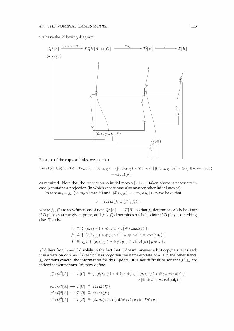
4.3. THE NOMINAL GAMESMODEL 113
we have the following diagram.
Q~aJAK〈id,φ〉 ; τ ;Tz ′
// TQ~a(JAK ⊗ JCK)Tσa // T 2JBK
µ // T JBK
(~a, iA(0))
∗
∗
∗
⊛
⊛
⊛a
a
a
iC
iC
iC
(~a, iA(0), iC ,⊛)
(∗,⊛)
⊛
Because of the copycat links, we see that
viewf(〈id, φ〉 ; τ ;T ζ ′ ;Tσa ;µ) ↾ (~a, iA(0)) = {[(~a, iA(0)) ∗ ⊛ a iC s] | [(~a, iA(0), iC) ∗ ⊛ s] ∈ viewf(σa)}
= viewf(σ) ,
as required. Note that the restriction to initial moves [~a, iA(0)] taken above is necessary in
case φ contains a projection (in which case it may also answer other initial moves).In casem0 = jA (som0 a store-H) and [(~a, iA(0)) ∗ ⊛m0 a iC ] ∈ σ, we have that
σ = strat(fa ∪ (f ′ \ f ′a)) ,
where fa, f′ are viewfunctions of typeQ~aJAK B T JBK, so that fa determines σ’s behaviour
if O plays a at the given point, and f ′ \ f ′a determines σ’s behaviour if O plays something
else. That is,
fa , { [(~a, iA(0)) ∗ ⊛ jA a iC s] ∈ viewf(σ) }
f ′a , { [(~a, iA(0)) ∗ ⊛ jA a s] | [⊛ ⊛ a s] ∈ viewf(idξ) }
f ′ , f ′a ∪ { [(~a, iA(0)) ∗ ⊛ jA y s] ∈ viewf(σ) | y 6= a } .
f ′ differs from viewf(σ) solely in the fact that it doesn’t answer a but copycats it instead;
it is a version of viewf(σ) which has forgotten the name-update of a. On the other hand,fa contains exactly the information for this update. It is not difficult to see that f ′, fa are
indeed viewfunctions. We now define
f ′′a : Q~aJAK B T JCK , { [(~a, iA(0)) ∗ ⊛ (iC ,⊛) s] | [(~a, iA(0)) ∗ ⊛ jA a iC s] ∈ fa
∨ [⊛ ⊛ s] ∈ viewf(idξ) }
σa : Q~aJAK B T JCK , strat(f ′′a )
σ′ : Q~aJAK B T JBK , strat(f ′)
σ′′ : Q~aJAK B T JBK , 〈∆, σa〉 ; τ ;T (id⊗φ ; τ) ;µ ;∼= ;Tσ′ ;µ .
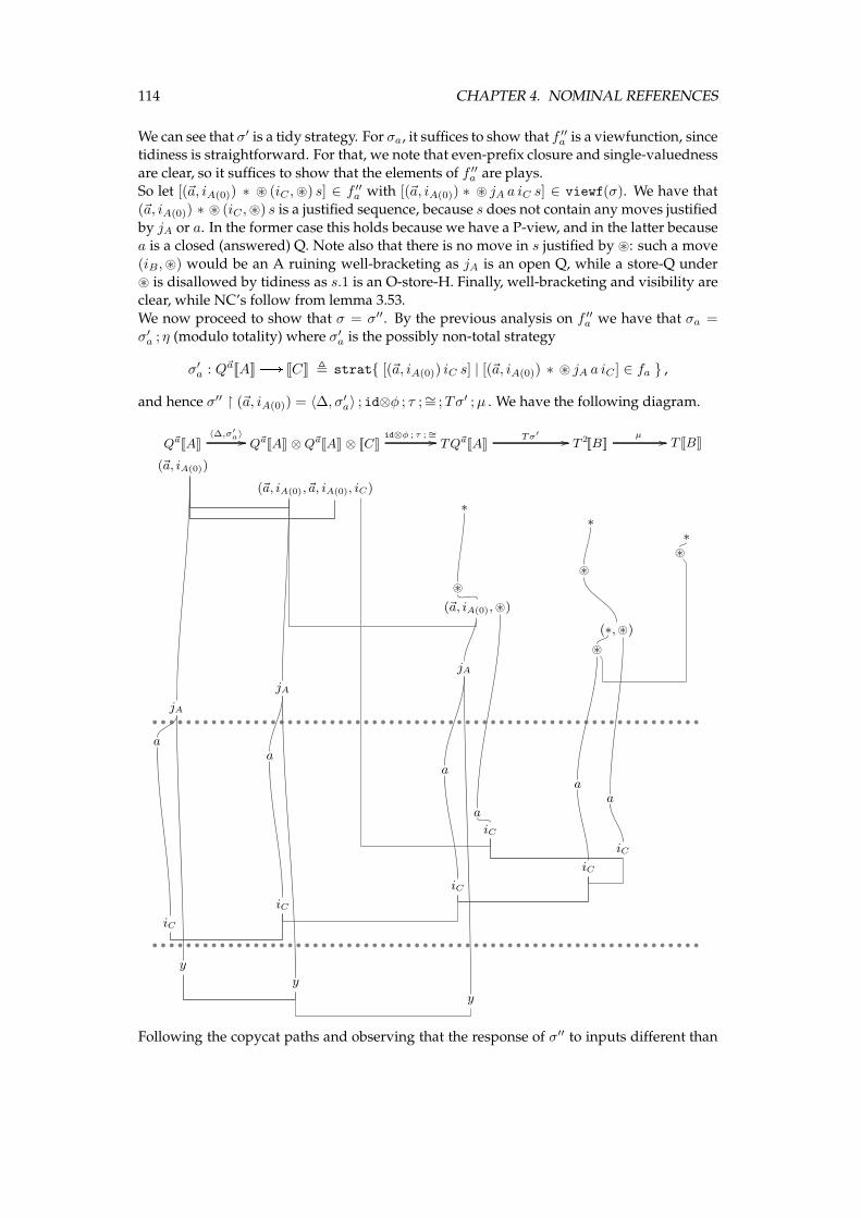
114 CHAPTER 4. NOMINAL REFERENCES
We can see that σ′ is a tidy strategy. For σa, it suffices to show that f ′′a is a viewfunction, since
tidiness is straightforward. For that, we note that even-prefix closure and single-valuedness
are clear, so it suffices to show that the elements of f ′′a are plays.
So let [(~a, iA(0)) ∗ ⊛ (iC ,⊛) s] ∈ f ′′a with [(~a, iA(0)) ∗ ⊛ jA a iC s] ∈ viewf(σ). We have that
(~a, iA(0)) ∗ ⊛ (iC ,⊛) s is a justified sequence, because s does not contain any moves justified
by jA or a. In the former case this holds because we have a P-view, and in the latter becausea is a closed (answered) Q. Note also that there is no move in s justified by ⊛: such a move
(iB,⊛) would be an A ruining well-bracketing as jA is an open Q, while a store-Q under⊛ is disallowed by tidiness as s.1 is an O-store-H. Finally, well-bracketing and visibility are
clear, while NC’s follow from lemma 3.53.
We now proceed to show that σ = σ′′. By the previous analysis on f ′′a we have that σa =
σ′a ; η (modulo totality) where σ′
a is the possibly non-total strategy
σ′a : Q~aJAK B JCK , strat{ [(~a, iA(0)) iC s] | [(~a, iA(0)) ∗ ⊛ jA a iC ] ∈ fa } ,
and hence σ′′ ↾ (~a, iA(0)) = 〈∆, σ′a〉 ; id⊗φ ; τ ;∼= ;Tσ′ ;µ . We have the following diagram.
Q~aJAK〈∆,σ′
a〉 // Q~aJAK ⊗ Q~aJAK ⊗ JCKid⊗φ ; τ ; ∼=// TQ~aJAK
Tσ′// T 2JBK
µ // T JBK
(~a, iA(0))
(~a, iA(0),~a, iA(0), iC)
∗
∗
∗
⊛⊛
⊛
(~a, iA(0), ⊛)
(∗, ⊛)
⊛jA
jA
jA
aa
aa
aa
iC
iC
iC
iC
iC
iC
y
y
y
Following the copycat paths and observing that the response of σ′′ to inputs different than
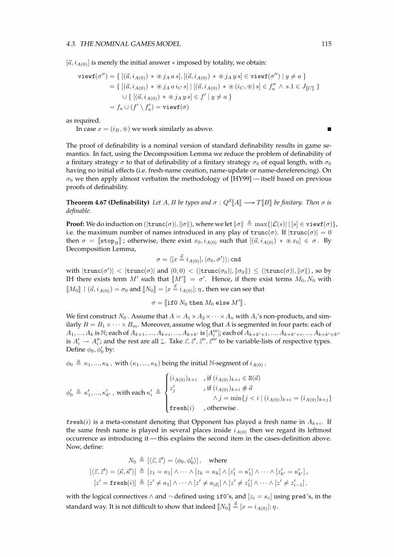
4.3. THE NOMINAL GAMESMODEL 115
[~a, iA(0)] is merely the initial answer ∗ imposed by totality, we obtain:
viewf(σ′′) = { [(~a, iA(0)) ∗ ⊛ jA a s], [(~a, iA(0)) ∗ ⊛ jA y s] ∈ viewf(σ′′) | y 6= a }
= { [(~a, iA(0)) ∗ ⊛ jA a iC s] | [(~a, iA(0)) ∗ ⊛ (iC ,⊛) s] ∈ f ′′a ∧ s.1 ∈ JJCK }
∪ { [(~a, iA(0)) ∗ ⊛ jA y s] ∈ f ′ | y 6= a }
= fa ∪ (f ′ \ f ′a) = viewf(σ)
as required.In case x = (iB,⊛) we work similarly as above. �
The proof of definability is a nominal version of standard definability results in game se-mantics. In fact, using the Decomposition Lemma we reduce the problem of definability of
a finitary strategy σ to that of definability of a finitary strategy σ0 of equal length, with σ0
having no initial effects (i.e. fresh-name creation, name-update or name-dereferencing). On
σ0 we then apply almost verbatim the methodology of [HY99]— itself based on previous
proofs of definability.
Theorem 4.67 (Definability) Let A,B be types and σ : Q~aJAK B T JBK be finitary. Then σ is
definable.
Proof: Wedo induction on (|trunc(σ)|, ‖σ‖), wherewe let ‖σ‖ , max{|L(s)| | [s] ∈ viewf(σ)},i.e. the maximum number of names introduced in any play of trunc(σ). If |trunc(σ)| = 0
then σ = JstopBK ; otherwise, there exist x0, iA(0) such that [(~a, iA(0)) ∗ ⊛ x0] ∈ σ . By
Decomposition Lemma,
σ = 〈[x~a= iA(0)], 〈σ0, σ
′〉〉; cnd
with |trunc(σ′)| < |trunc(σ)| and (0, 0) < (|trunc(σ0)|, ‖σ0‖) ≤ (|trunc(σ)|, ‖σ‖) , so by
IH there exists term M ′ such that JM ′K = σ′. Hence, if there exist terms M0, N0 with
JM0K ↾ (~a, iA(0)) = σ0 and JN0K = [x~a= iA(0)]; η , then we can see that
σ = Jif0 N0 thenM0 elseM′K .
We first constructN0 . Assume thatA = A1×A2×· · ·×An withAi’s non-products, and sim-ilarly B = B1 × · · · ×Bm. Moreover, assume wlog that A is segmented in four parts: each of
A1, ..., Ak isN; each ofAk+1, ..., Ak+i, ..., Ak+k′ is [A′′′i ]; each ofAk+k′+1, ..., Ak+k′+i, ..., Ak+k′+k′′
is A′i → A′′
i ; and the rest are all 1. Take ~z, ~z′, ~z′′, ~z′′′ to be variable-lists of respective types.Define φ0, φ
′0 by:
φ0 , κ1, ..., κk , with (κ1, ..., κk) being the initial N-segment of iA(0) ,
φ′0 , κ′1, ..., κ′k′ , with each κ′i ,
(iA(0))k+i , if (iA(0))k+i ∈ S(~a)
z′j , if (iA(0))k+i # ~a
∧ j = min{j < i | (iA(0))k+i = (iA(0))k+j}
fresh(i) , otherwise .
fresh(i) is a meta-constant denoting that Opponent has played a fresh name in Ak+i. If
the same fresh name is played in several places inside iA(0) then we regard its leftmostoccurrence as introducing it— this explains the second item in the cases-definition above.
Now, define:
N0 , [〈~z, ~z′〉 = 〈φ0, φ′0〉] , where
[〈~z, ~z′〉 = 〈~κ,~κ′〉] , [z1 = κ1] ∧ · · · ∧ [zk = κk] ∧ [z′1 = κ′1] ∧ · · · ∧ [z′k′ = κ′k′ ] ,
[z′ = fresh(i)] , [z′ 6= a1] ∧ · · · ∧ [z′ 6= a|~a|] ∧ [z′ 6= z′1] ∧ · · · ∧ [z′ 6= z′i−1] ,
with the logical connectives ∧ and ¬ defined using if0’s, and [zi = κi] using pred ’s, in the
standard way. It is not difficult to show that indeed JN0K~a= [x = iA(0)]; η .
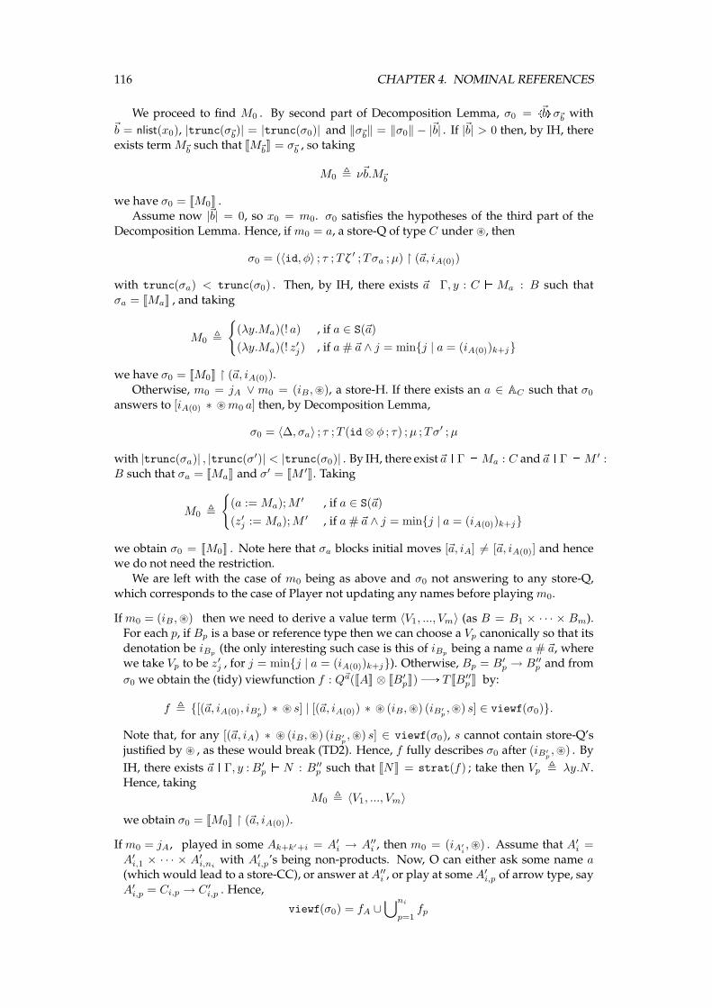
116 CHAPTER 4. NOMINAL REFERENCES
We proceed to find M0 . By second part of Decomposition Lemma, σ0 = \~b℄σ~b with~b = nlist(x0), |trunc(σ~b)| = |trunc(σ0)| and ‖σ~b‖ = ‖σ0‖ − |~b| . If |~b| > 0 then, by IH, thereexists termM~b such that JM~bK = σ~b , so taking
M0 , ν~b.M~b
we have σ0 = JM0K .Assume now |~b| = 0, so x0 = m0. σ0 satisfies the hypotheses of the third part of the
Decomposition Lemma. Hence, ifm0 = a, a store-Q of type C under ⊛, then
σ0 = (〈id, φ〉 ; τ ;T ζ ′ ;Tσa ;µ) ↾ (~a, iA(0))
with trunc(σa) < trunc(σ0) . Then, by IH, there exists ~a ^ Γ, y : C_Ma : B such that
σa = JMaK , and taking
M0 ,
{
(λy.Ma)(! a) , if a ∈ S(~a)
(λy.Ma)(! z′j) , if a# ~a ∧ j = min{j | a = (iA(0))k+j}
we have σ0 = JM0K ↾ (~a, iA(0)).
Otherwise, m0 = jA ∨ m0 = (iB,⊛), a store-H. If there exists an a ∈ AC such that σ0
answers to [iA(0) ∗ ⊛m0 a] then, by Decomposition Lemma,
σ0 = 〈∆, σa〉 ; τ ;T (id⊗ φ ; τ) ;µ ;Tσ′ ;µ
with |trunc(σa)| , |trunc(σ′)| < |trunc(σ0)| . By IH, there exist~a ^ Γ_Ma : C and~a ^ Γ_M ′ :
B such that σa = JMaK and σ′ = JM ′K. Taking
M0 ,
{
(a := Ma);M′ , if a ∈ S(~a)
(z′j := Ma);M′ , if a# ~a ∧ j = min{j | a = (iA(0))k+j}
we obtain σ0 = JM0K . Note here that σa blocks initial moves [~a, iA] 6= [~a, iA(0)] and hencewe do not need the restriction.
We are left with the case of m0 being as above and σ0 not answering to any store-Q,
which corresponds to the case of Player not updating any names before playingm0.
Ifm0 = (iB,⊛) then we need to derive a value term 〈V1, ..., Vm〉 (as B = B1 × · · · × Bm).For each p, if Bp is a base or reference type then we can choose a Vp canonically so that its
denotation be iBp(the only interesting such case is this of iBp
being a name a# ~a, wherewe take Vp to be z′j , for j = min{j | a = (iA(0))k+j}). Otherwise, Bp = B′
p → B′′p and from
σ0 we obtain the (tidy) viewfunction f : Q~a(JAK ⊗ JB′pK)B T JB′′
p K by:
f , {[(~a, iA(0), iB′p) ∗ ⊛ s] | [(~a, iA(0)) ∗ ⊛ (iB,⊛) (iB′
p,⊛) s] ∈ viewf(σ0)}.
Note that, for any [(~a, iA) ∗ ⊛ (iB,⊛) (iB′p,⊛) s] ∈ viewf(σ0), s cannot contain store-Q’s
justified by ⊛ , as these would break (TD2). Hence, f fully describes σ0 after (iB′p,⊛) . By
IH, there exists ~a ^ Γ, y :B′p_N : B′′
p such that JNK = strat(f) ; take then Vp , λy.N .Hence, taking
M0 , 〈V1, ..., Vm〉
we obtain σ0 = JM0K ↾ (~a, iA(0)).
Ifm0 = jA, played in some Ak+k′+i = A′i → A′′
i , then m0 = (iA′i,⊛) . Assume that A′
i =
A′i,1 × · · · × A′
i,niwith A′
i,p’s being non-products. Now, O can either ask some name a(which would lead to a store-CC), or answer at A′′
i , or play at some A′i,p of arrow type, say
A′i,p = Ci,p → C′
i,p . Hence,
viewf(σ0) = fA ∪⋃ni
p=1fp
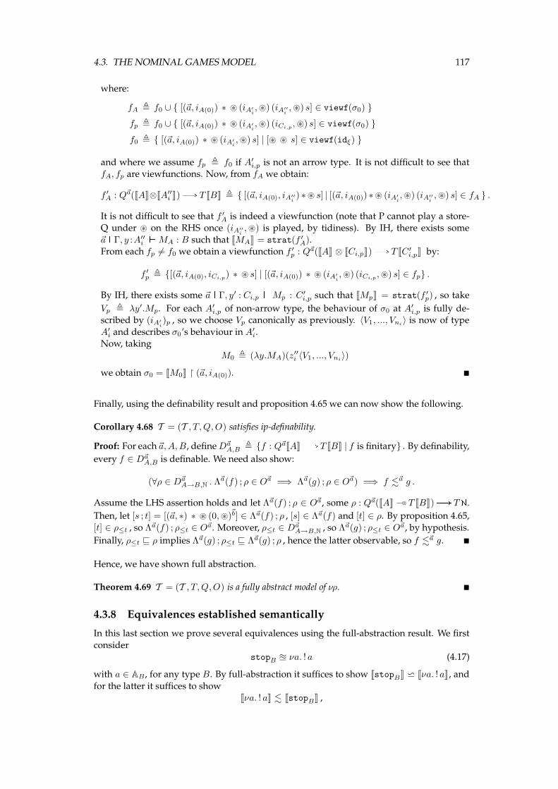
4.3. THE NOMINAL GAMESMODEL 117
where:
fA , f0 ∪ { [(~a, iA(0)) ∗ ⊛ (iA′i,⊛) (iA′′
i,⊛) s] ∈ viewf(σ0) }
fp , f0 ∪ { [(~a, iA(0)) ∗ ⊛ (iA′i,⊛) (iCi,p
,⊛) s] ∈ viewf(σ0) }
f0 , { [(~a, iA(0)) ∗ ⊛ (iA′i,⊛) s] | [⊛ ⊛ s] ∈ viewf(idξ) }
and where we assume fp , f0 if A′i,p is not an arrow type. It is not difficult to see that
fA, fp are viewfunctions. Now, from fA we obtain:
f ′A : Q~a(JAK⊗JA′′
i K)B T JBK , { [(~a, iA(0), iA′′i) ∗⊛ s] | [(~a, iA(0)) ∗⊛ (iA′
i,⊛) (iA′′
i,⊛) s] ∈ fA } .
It is not difficult to see that f ′A is indeed a viewfunction (note that P cannot play a store-
Q under ⊛ on the RHS once (iA′′i,⊛) is played, by tidiness). By IH, there exists some
~a ^ Γ, y :A′′i _MA : B such that JMAK = strat(f ′
A).From each fp 6= f0 we obtain a viewfunction f ′
p : Q~a(JAK ⊗ JCi,pK)B T JC′i,pK by:
f ′p , {[(~a, iA(0), iCi,p
) ∗ ⊛ s] | [(~a, iA(0)) ∗ ⊛ (iA′i,⊛) (iCi,p
,⊛) s] ∈ fp} .
By IH, there exists some ~a ^ Γ, y′ : Ci,p_Mp : C′i,p such that JMpK = strat(f ′
p) , so take
Vp , λy′.Mp. For each A′i,p of non-arrow type, the behaviour of σ0 at A′
i,p is fully de-scribed by (iA′
i)p , so we choose Vp canonically as previously. 〈V1, ..., Vni
〉 is now of type
A′i and describes σ0’s behaviour in A
′i.
Now, taking
M0 , (λy.MA)(z′′i 〈V1, ..., Vni〉)
we obtain σ0 = JM0K ↾ (~a, iA(0)). �
Finally, using the definability result and proposition 4.65 we can now show the following.
Corollary 4.68 T = (T , T,Q,O) satisfies ip-definability.
Proof: For each~a,A,B, defineD~aA,B , {f : Q~aJAK B T JBK | f is finitary} . By definability,
every f ∈ D~aA,B is definable. We need also show:
(∀ρ ∈ D~aA→B,N . Λ~a(f) ; ρ ∈ O~a =⇒ Λ~a(g) ; ρ ∈ O~a) =⇒ f .~a g .
Assume the LHS assertion holds and let Λ~a(f) ; ρ ∈ O~a, some ρ : Q~a(JAK −−⊗ T JBK) B TN.Then, let [s ; t] = [(~a, ∗) ∗ ⊛ (0,⊛)
~b] ∈ Λ~a(f) ; ρ , [s] ∈ Λ~a(f) and [t] ∈ ρ. By proposition 4.65,
[t] ∈ ρ≤t , so Λ~a(f) ; ρ≤t ∈ O~a. Moreover, ρ≤t ∈ D~aA→B,N , so Λ~a(g) ; ρ≤t ∈ O~a, by hypothesis.
Finally, ρ≤t ⊑ ρ implies Λ~a(g) ; ρ≤t ⊑ Λ~a(g) ; ρ , hence the latter observable, so f .~a g. �
Hence, we have shown full abstraction.
Theorem 4.69 T = (T , T,Q,O) is a fully abstract model of νρ. �
4.3.8 Equivalences established semantically
In this last section we prove several equivalences using the full-abstraction result. We first
consider
stopB ≅ νa. ! a (4.17)
with a ∈ AB , for any type B. By full-abstraction it suffices to show JstopBK ⋍ Jνa. ! aK, and
for the latter it suffices to showJνa. ! aK . JstopBK ,
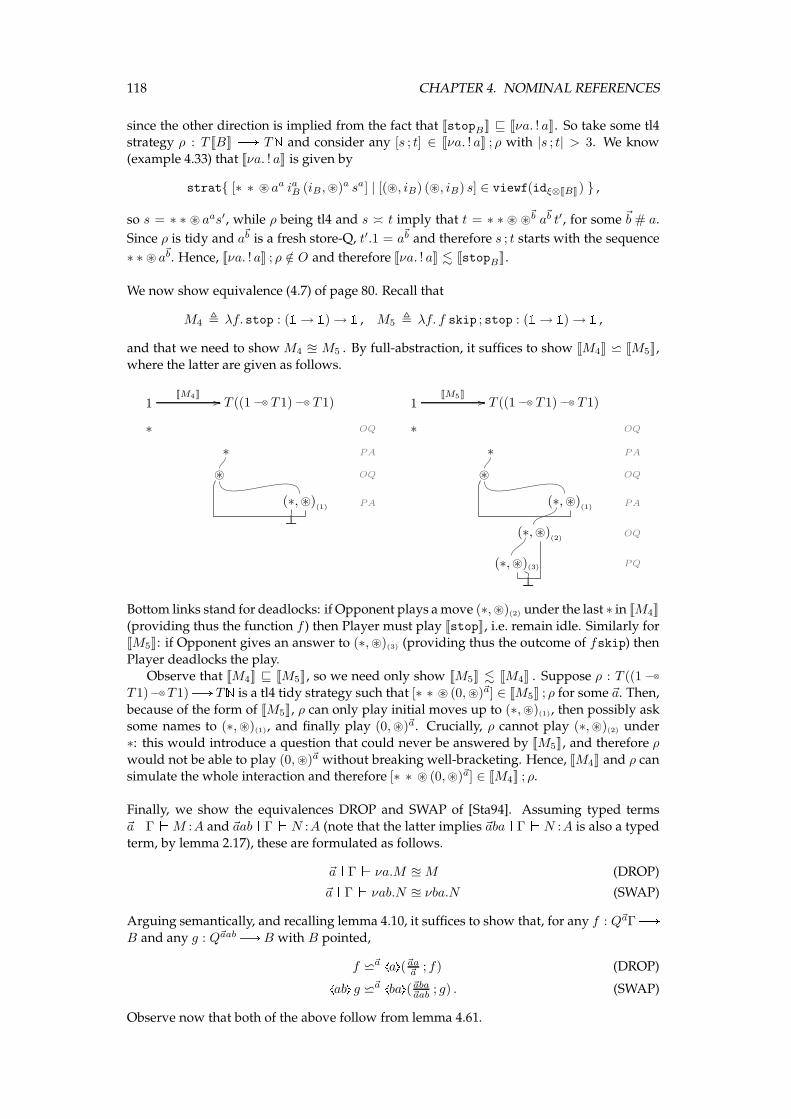
118 CHAPTER 4. NOMINAL REFERENCES
since the other direction is implied from the fact that JstopBK ⊑ Jνa. ! aK. So take some tl4strategy ρ : T JBK B TN and consider any [s ; t] ∈ Jνa. ! aK ; ρ with |s ; t| > 3. We know
(example 4.33) that Jνa. ! aK is given by
strat{ [∗ ∗ ⊛ aa iaB (iB,⊛)a sa] | [(⊛, iB) (⊛, iB) s] ∈ viewf(idξ⊗JBK) } ,
so s = ∗ ∗ ⊛ aas′, while ρ being tl4 and s ≍ t imply that t = ∗ ∗ ⊛ ⊛~b a~b t′, for some ~b # a.
Since ρ is tidy and a~b is a fresh store-Q, t′.1 = a
~b and therefore s ; t starts with the sequence
∗ ∗ ⊛ a~b. Hence, Jνa. ! aK ; ρ /∈ O and therefore Jνa. ! aK . JstopBK.
We now show equivalence (4.7) of page 80. Recall that
M4 , λf. stop : (1→ 1) → 1 , M5 , λf. f skip ; stop : (1 → 1) → 1 ,and that we need to showM4 ≅ M5 . By full-abstraction, it suffices to show JM4K ⋍ JM5K,
where the latter are given as follows.
1JM4K // T ((1 −−⊗ T 1) −−⊗ T 1)
∗ OQ
∗ PA
⊛ OQ
(
⊥
∗,⊛)(1) PA
1JM5K // T ((1 −−⊗ T 1) −−⊗ T 1)
∗ OQ
∗ PA
⊛ OQ
(∗,⊛)(1) PA
(∗,⊛)(2)
OQ
(∗,⊛)
⊥
(3) PQ
Bottom links stand for deadlocks: if Opponent plays amove (∗,⊛)(2) under the last ∗ in JM4K
(providing thus the function f ) then Player must play JstopK, i.e. remain idle. Similarly forJM5K: if Opponent gives an answer to (∗,⊛)(3) (providing thus the outcome of fskip) then
Player deadlocks the play.Observe that JM4K ⊑ JM5K, so we need only show JM5K . JM4K . Suppose ρ : T ((1 −−⊗
T 1) −−⊗T 1)B TN is a tl4 tidy strategy such that [∗ ∗ ⊛ (0,⊛)~a] ∈ JM5K ; ρ for some ~a. Then,
because of the form of JM5K, ρ can only play initial moves up to (∗,⊛)(1), then possibly asksome names to (∗,⊛)(1), and finally play (0,⊛)~a. Crucially, ρ cannot play (∗,⊛)(2) under
∗: this would introduce a question that could never be answered by JM5K, and therefore ρ
would not be able to play (0,⊛)~a without breaking well-bracketing. Hence, JM4K and ρ cansimulate the whole interaction and therefore [∗ ∗ ⊛ (0,⊛)~a] ∈ JM4K ; ρ.
Finally, we show the equivalences DROP and SWAP of [Sta94]. Assuming typed terms
~a ^ Γ_M :A and ~aab ^ Γ_N :A (note that the latter implies ~aba ^ Γ_N :A is also a typed
term, by lemma 2.17), these are formulated as follows.
~a ^ Γ_ νa.M ≅ M (DROP)
~a ^ Γ_ νab.N ≅ νba.N (SWAP)
Arguing semantically, and recalling lemma 4.10, it suffices to show that, for any f : Q~aΓ BB and any g : Q~aabB B with B pointed,
f ⋍~a \a℄(~aa~a ; f) (DROP)\ab℄ g ⋍~a \ba℄(~aba~aab ; g) . (SWAP)
Observe now that both of the above follow from lemma 4.61.
Chapter 5
Nominal Exceptions
In this chapter we examine extensions of the sν-calculus in which names can be raised and
handled as exceptions. Exceptions are a prevalent feature of programming languages forraising and handling eccentric program behaviour, and more generally for manipulating
the flow of control. It is a key feature, for example, of ML, Java and C++. The raising
of an exception forces a program to escape out of its context and to the nearest availableexception-handler. Thus, exceptions provide a means of (an effect for) overriding nested
behaviour of functional programs.
We start with a simple extension of the sν-calculus, the νε-calculus, of which we brieflyexamine the syntax and abstract categorical semantics. The main focus, though, is on the
νερ-calculus, the extension of νρ with nominal exceptions. For νερ we carry out a simi-lar analysis as with νρ in the previous chapter (factoring out material covered previously
where possible), and thus construct a fully abstract semantics in nominal games. The con-
struction combines elegantly the use of an exception monad with the nominal games settingwhere atoms are used (also) for exception names. We obtain a model of νερ in (innocent,
well-bracketed) nominal games, which we then restrict to strategies with ‘disciplined’ ex-ceptional behaviour (x-tidy strategies) to the effect of obtaining a fully abstract model.
A fully abstract model for a language with exceptions and ground-type references was
constructed in [Lai01]. In rough terms, the model of [Lai01] allows for jumps in the prece-dence with which a program answers questions posed by the environment (i.e. it mildens
the well-bracketing condition), thus translating in the semantical universe the override ofnested behaviour. This yields a description of the exception effect that is both accurate and
intuitive. However, the modelling of exceptions themselves is not nominal but rather based
on the ‘object-oriented’ approach which encodes exceptions as products of raise/handletype. Therefore, “bad” constructors are included in the syntax, that is, the language exam-
ined includes bad exceptions (and also bad variables). Another point of difference betweenthe two languages is that the one of [Lai01], being an extension of Idealized Algol [Rey81],
is call-by-name with block-structured exceptions and references.
5.1 The νε-calculus
Exceptions are a mechanism allowing program control to jump out of the current context
and to the nearest handler. In the calculus we examine now, exceptions are terms of type E.These can be raised and handled, and their closed values are given by names. The latter aretaken from a set of atoms
Ae ∈ (Ai)i∈ω
and hence the calculus is an extension of sν with names used for exceptions.
Definition 5.1 The νε-calculus is a functional calculus of nominal exceptions. Its types,
119
120 CHAPTER 5. NOMINAL EXCEPTIONS
terms and values are given as follows.
TY ∋ A,B ::= N | A→ B | A×B | E
TE ∋M,N ::= x | λx.M |M N | 〈M,N〉 | fstM | sndN λ-calculus
| n | predM | succN arithmetic
| if0M thenN1 elseN2 if then else
| a | νa.M | [M = N ] ν-calculus (a ∈ Ae)
| raiseM raise exception
| tryN1 handleM =>N2 try/handle exception
VA ∋ V,W ::= x | n | a | λx.M | 〈V,W 〉
The typing system involves (as before) terms in environments ~a^Γ; the main typing rulesare the following.
a ∈ ~a~a ^ Γ_ a : E
~aa ^ Γ_M : B
~a ^ Γ_ νa.M : B
~a ^ Γ_M : E ~a ^ Γ_N : E
~a ^ Γ_ [M = N ] : N
~a ^ Γ_M : E
~a ^ Γ_ raiseM : A
~a ^ Γ_M : E ~a ^ Γ_N1, N2 : A
~a ^ Γ_ tryN1 handleM =>N2 : A
N
Observe that TE and VA are strong nominal sets. Regarding bound names and variables,the same definitions and conventions as in the case of the sν-calculus are in effect. Note that
raised exceptions can have any type— even exception-type. Thus, for example, both the
following terms can have type E,
M1 , a , M2 , raise a ,
but they are quite different: the former is a value of exception-type, while the latter is clearly
non-value.
The operational semantics is defined by means of a small-step reduction relation, whereterms reduce in name-list environments containing the names created thus far in the com-
putation.
Definition 5.2 Reduction in the νε-calculus involves sν-calculus reduction rules and rulesfor exceptions. The latter set of rules is given below.
HL~a` try (raise a) handle a => N −−→ ~a` N
VHL~a` try V handle a => N −−→ ~a` V
NHL a6=b
~a` try (raise b) handle a =>N −−→ ~a` raise b
XPN~a` Z[raise a] −−→ ~a` raise a
CTX~a`M −−→ ~a′ `M ′
~a` E[M ] −−→ ~a′ ` E[M ′]
Unhandled evaluation contexts Z are of the forms:
(λx.N) , N , 〈 , N〉 , 〈V, 〉 , fst , snd , if0 thenN1 elseN2 ,
succ , pred , [ = N ] , [a = ] , raise , tryN1 handle =>N2 .
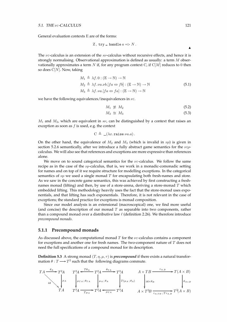
5.1. THE νε-CALCULUS 121
General evaluation contexts E are of the forms:
Z , try handle a =>N .N
The νε-calculus is an extension of the sν-calculus without recursive effects, and hence it is
strongly normalising. Observational approximation is defined as usually: a termM obser-vationally approximates a term N if, for any program context C, if C[M ] reduces to 0 then
so does C[N ]. Now, taking
M1 , λf. 0 : (E → N) → N
M2 , λf. νa.νb.[fa⇔ fb] : (E → N) → N
M3 , λf. νa.[fa⇔ fa] : (E → N) → N
(5.1)
we have the following equivalences/inequivalences in νε.
M1 6≅ M2 (5.2)
M2 ≅ M3 (5.3)
M1 and M2, which are equivalent in sν, can be distinguished by a context that raises an
exception as soon as f is used, e.g. the context
C , (λx. raise νa.a) .
On the other hand, the equivalence of M2 and M3 (which is invalid in νρ) is given in
section 5.2.6 semantically, after we introduce a fully abstract game semantics for the νερ-
calculus. Wewill also see that references and exceptions aremore expressive than referencesalone.
We move on to sound categorical semantics for the νε-calculus. We follow the same
recipe as in the case of the νρ-calculus, that is, we work in a monadic-comonadic settingfor names and on top of it we require structure for modelling exceptions. In the categorical
semantics of νρ we used a single monad T for encapsulating both fresh-names and store.As we saw in the concrete game semantics, this was achieved by first constructing a fresh-
names monad (lifting) and then, by use of a store-arena, deriving a store-monad T which
embedded lifting. This methodology heavily uses the fact that the store-monad uses expo-nentials, and that lifting has such exponentials. Therefore, it is not relevant in the case of
exceptions; the standard practice for exceptions is monad composition.Since our model analysis is an extensional (macroscopical) one, we find more useful
(and concise) the description of our monad T as separable into two components, rather
than a compound monad over a distributive law ℓ (definition 2.26). We therefore introduceprecompound monads.
5.1.1 Precompound monads
As discussed above, the computational monad T for the νε-calculus contains a componentfor exceptions and another one for fresh names. The two-component nature of T does not
need the full specifications of a compound monad for its description.
Definition 5.3 A strong monad (T, η, µ, τ) is precompound if there exists a natural transfor-
mation θ : T B T 2 such that the following diagrams commute.
TAθA //
id
AAA
AAAA
AAAA
T 2A
µA
��TA
T 3A
µT A ; θT A
��
T 2A
µA ; θA
��
TθAoo θTA // T 3A
T (µA ; θA)
��T 3A
TµA
// T 2A T 3AµT A
oo
A× TBτA,B //
id×θB
��
T (A×B)
θA×B
��A× T 2B
τA,TB ;TτA,B
// T 2(A×B)
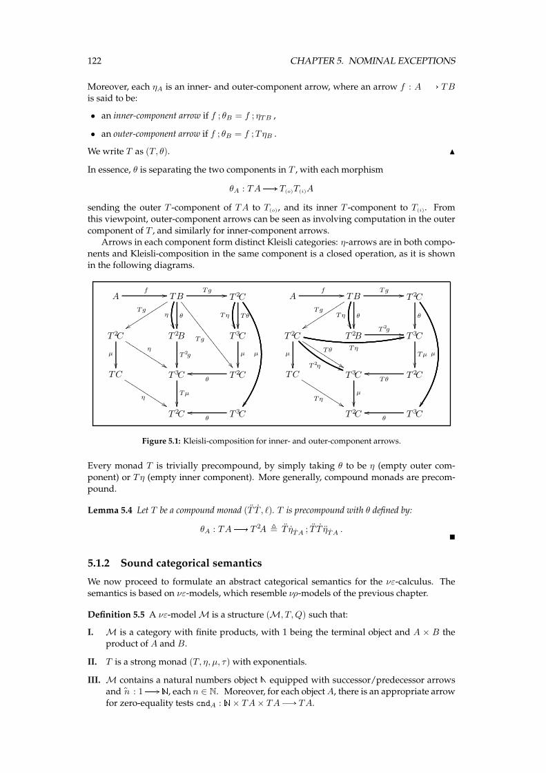
122 CHAPTER 5. NOMINAL EXCEPTIONS
Moreover, each ηA is an inner- and outer-component arrow, where an arrow f : AB TB
is said to be:
• an inner-component arrow if f ; θB = f ; ηTB ,
• an outer-component arrow if f ; θB = f ;TηB .
We write T as (T, θ). N
In essence, θ is separating the two components in T , with each morphism
θA : TAB T(o)T(i)A
sending the outer T -component of TA to T(o), and its inner T -component to T(i). From
this viewpoint, outer-component arrows can be seen as involving computation in the outer
component of T , and similarly for inner-component arrows.Arrows in each component form distinct Kleisli categories: η-arrows are in both compo-
nents and Kleisli-composition in the same component is a closed operation, as it is shownin the following diagrams.
Af // TB
Tg //
Tg
��88
88
88
88
88
88
88
88
88
8
θ
��η
��
Tg
yysssssssssssT 2C
Tθ
��Tη
��
µ
��
T 2C
µ
��
η
%%KKKKKKKKKKK T 2B
T 2g
��
T 3C
µ
��TC
η%%KKKKKKKKKKK T 3C
Tµ
��
T 2Cθ
oo
T 2C T 3Cθ
oo
Af // TB
Tg //
Tg
yysssssssssss
θ
��Tη
��
T 2C
θ
��
µ
��
T 2C
µ
�� T 2η ))
Tη
22
Tθ
%%KKKKKKKKKKK T 2BT 2g // T 3C
Tµ
��TC
Tη%%KKKKKKKKKKK T 3C
µ
��
T 2CTθ
oo
T 2C T 3Cθ
oo
Figure 5.1: Kleisli-composition for inner- and outer-component arrows.
Every monad T is trivially precompound, by simply taking θ to be η (empty outer com-
ponent) or Tη (empty inner component). More generally, compound monads are precom-
pound.
Lemma 5.4 Let T be a compound monad (T T , ℓ). T is precompound with θ defined by:
θA : TAB T 2A , T ηTA ; T T ηTA .�
5.1.2 Sound categorical semantics
We now proceed to formulate an abstract categorical semantics for the νε-calculus. The
semantics is based on νε-models, which resemble νρ-models of the previous chapter.
Definition 5.5 A νε-model M is a structure (M, T,Q) such that:
I. M is a category with finite products, with 1 being the terminal object and A × B theproduct of A and B.
II. T is a strong monad (T, η, µ, τ) with exponentials.
III. M contains a natural numbers object N equipped with successor/predecessor arrowsand
bn : 1B N, each n ∈ N. Moreover, for each objectA, there is an appropriate arrow
for zero-equality tests cndA : N× TA× TAB TA.
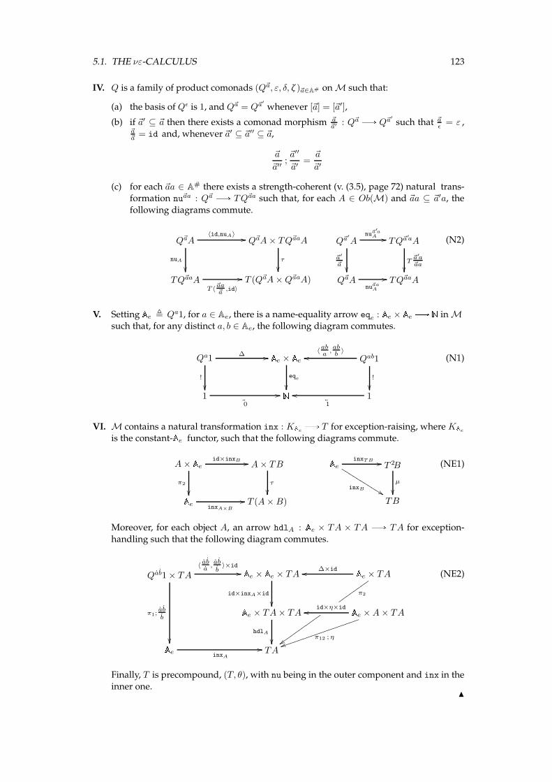
5.1. THE νε-CALCULUS 123
IV. Q is a family of product comonads (Q~a, ε, δ, ζ )~a∈A# on M such that:
(a) the basis of Qǫ is 1, and Q~a = Q~a′
whenever [~a] = [~a′],
(b) if ~a′ ⊆ ~a then there exists a comonad morphism ~a~a′ : Q~a B Q~a
′
such that ~aǫ = ε ,~a~a = id and, whenever ~a′ ⊆ ~a′′ ⊆ ~a,
~a
~a′′;~a′′
~a′=~a
~a′
(c) for each ~aa ∈ A# there exists a strength-coherent (v. (3.5), page 72) natural trans-formation nu~aa : Q~a B TQ~aa such that, for each A ∈ Ob(M) and ~aa ⊆ ~a′a, the
following diagrams commute.
Q~aA
nuA
��
〈id,nuA〉 // Q~aA× TQ~aaA
τ
��TQ~aaA
T 〈~aa~a ,id〉
// T (Q~aA×Q~aaA)
Q~a′
Anu
~a′aA //
~a′
~a��
TQ~a′aA
T~a′a~aa
��Q~aA
nu~aaA
// TQ~aaA
(N2)
V. Setting Ae , Qa1, for a ∈ Ae, there is a name-equality arrow eqe : Ae × Ae B N in Msuch that, for any distinct a, b ∈ Ae, the following diagram commutes.
Qa1∆ //
!
��
Ae × Aeeqe
��
Qab1〈aba ,
abb 〉
oo
!
��1 b
0
// N 1b1
oo
(N1)
VI. M contains a natural transformation inx : KAeB T for exception-raising, where KAe
is the constant-Ae functor, such that the following diagrams commute.
A× Ae id×inxB //
π2
��
A× TB
τ
��AeinxA×B
// T (A×B)
Ae inxT B //
inxB %%KKKKKKKKKKK T 2B
µ
��TB
(NE1)
Moreover, for each object A, an arrow hdlA : Ae × TA × TA B TA for exception-
handling such that the following diagram commutes.
Qab1 × TA〈aba ,
abb〉×id
//
π1;abb
��
Ae × Ae × TA
id×inxA×id
��
Ae × TA∆×idoo
vvvvvvvv
π2
zzvvvvvvvvvvvAe × TA× TA
hdlA
��
Ae ×A× TAid×η×idoo
π12 ; ηuujjjjjjjjjjjjjjjjjjAe
inxA
// TA
(NE2)
Finally, T is precompound, (T, θ), with nu being in the outer component and inx in the
inner one.N
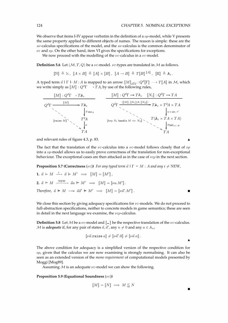
124 CHAPTER 5. NOMINAL EXCEPTIONS
We observe that items I-IV appear verbatim in the definition of a νρ-model, while V presentsthe same property applied to different objects of names. The reason is simple: these are the
sν-calculus specifications of the model, and the sν-calculus is the common denominator ofνε and νρ. On the other hand, item VI gives the specifications for exceptions.
We now proceed with the modelling of the νε-calculus in a νε-model.
Definition 5.6 Let (M, T,Q) be a νε-model. νε-types are translated inM as follows.
JNK , N , JA×BK , JAK × JBK , JA→ BK , T JBK JAK , JEK , Ae .A typed term ~a ^ Γ_M :A is mapped to an arrow JMK
~a^Γ :Q~aJΓK B T JAK in M, which
we write simply as JMK : Q~aΓ B TA, by use of the following rules,
JMK : Q~aΓ A TAeQ~aΓ
Jraise MK
##HH
HH
HH
HH
HH
JMK // TAeTinxA
��T 2A
µ
��TA
JMK : Q~aΓ A TAe JNiK : Q~aΓ A TA
Q~aΓ
Jtry N1 handle M => N2K
''NN
NN
NN
NN
NN
NN
N
〈JMK, JN1K;θ, JN2K〉 // TAe × T 2A× TA
ψ×id ; τ ′
��T (Ae × TA× TA)
ThdlA ;µ
��TA
and relevant rules of figure 4.3, p. 83. N
The fact that the translation of the νε-calculus into a νε-model follows closely that of νρinto a νρ-model allows us to easily prove correctness of the translation for non-exceptional
behaviour. The exceptional cases are then attacked as in the case of νερ in the next section.
Proposition 5.7 (Correctness (νε)) For any typed term ~a ^ Γ_M : A and any r 6= NEW,
1. ~a`Mr
−−→ ~a`M ′ =⇒ JMK = JM ′K ,
2. ~a`MNEW
−−−−−→ ~aa`M ′ =⇒ JMK = Jνa.M ′K .
Therefore, ~a`M −→→ ~a~a′ `M ′ =⇒ JMK = Jν~a′.M ′K . �
We close this section by giving adequacy specifications for νε-models. We do not proceed to
full-abstraction specifications, neither to concrete models in game semantics; these are seen
in detail in the next language we examine, the νερ-calculus.
Definition 5.8 LetM be a νε-model and J K be the respective translation of the νε-calculus.M is adequate if, for any pair of states ~a,~a′, any n 6= 0 and any a ∈ Ae,
Jν~a.raise aK 6= Jν~a′.0K 6= Jν~a.nK .N
The above condition for adequacy is a simplified version of the respective condition for
νρ, given that the calculus we are now examining is strongly normalising. It can also beseen as an extended version of the mono requirement of computational models presented by
Moggi [Mog89].
Assuming M is an adequate νε-model we can show the following.
Proposition 5.9 (Equational Soundness (νε))
JMK = JNK =⇒ M / N�
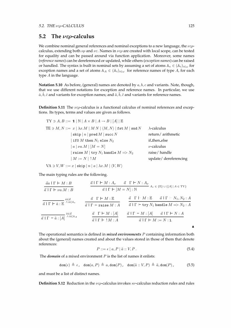
5.2. THE νερ-CALCULUS 125
5.2 The νερ-calculus
We combine nominal general references and nominal exceptions to a new language, the νερ-calculus, extending both νρ and νε. Names in νερ are created with local scope, can be tested
for equality and can be passed around via function application. Moreover, some names(reference names) can be dereferenced or updated, while others (exception names) can be raised
or handled. The syntax is built in nominal sets by assuming a set of atoms Ae ∈ (Ai)i∈ω for
exception names and a set of atoms AA ∈ (Ai)i∈ω for reference names of type A, for eachtype A in the language.
Notation 5.10 As before, (general) names are denoted by a, b, c and variants. Note, though,
that we use different notations for exception and reference names. In particular, we use
a, b, c and variants for exception names; and a, b, c and variants for reference names.
Definition 5.11 The νερ-calculus is a functional calculus of nominal references and excep-
tions. Its types, terms and values are given as follows.
TY ∋ A,B ::= 1 | N | A×B | A→ B | [A] | E
TE ∋M,N ::= x | λx.M |M N | 〈M,N〉 | fstM | sndN λ-calculus
| skip | n | predM | succN return/ arithmetic
| if0M thenN1 elseN2 if then else
| a | νa.M | [M = N ] ν-calculus
| raiseM | try N1 handleM => N2 raise/ handle
|M := N | !M update/ dereferencing
VA ∋ V,W ::= x | skip | n | a | λx.M | 〈V,W 〉
The main typing rules are the following.
~aa ^ Γ_M : B
~a ^ Γ_ νa.M : B
~a ^ Γ_M : Aν ~a ^ Γ_N : AνAν ∈ {E} ∪ {[A] |A ∈ TY}
~a ^ Γ_ [M = N ] : N
a∈~a∧ a∈Ae~a ^ Γ_ a : E
~a ^ Γ_M : E
~a ^ Γ_ raiseM : A
~a ^ Γ_M : E ~a ^ Γ_N1, N2 : A
~a ^ Γ_ try N1 handleM => N2 : A
a∈~a∧ a∈AA~a ^ Γ_ a : [A]
~a ^ Γ_M : [A]
~a ^ Γ_ !M : A
~a ^ Γ_M : [A] ~a ^ Γ_N : A
~a ^ Γ_M := N : 1N
The operational semantics is defined inmixed environments P containing information both
about the (general) names created and about the values stored in those of them that denotereferences:
P ::= ǫ | a, P | a :: V, P . (5.4)
The domain of a mixed environment P is the list of names it enlists:
dom(ǫ) , ǫ , dom(a, P ) , a, dom(P ) , dom(a :: V, P ) , a, dom(P ) , (5.5)
and must be a list of distinct names.
Definition 5.12 Reduction in the νερ-calculus invokes sν-calculus reduction rules and rules
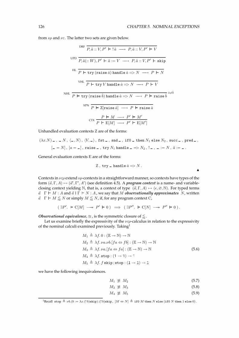
126 CHAPTER 5. NOMINAL EXCEPTIONS
from νρ and νε. The latter two sets are given below.
DRFP, a :: V, P ′ ` ! a −−→ P, a :: V, P ′ ` V
UPDP, a(:: W ), P ′ ` a := V −−→ P, a :: V, P ′ ` skip
HLP ` try (raise a) handle a => N −−→ P ` N
VHLP ` try V handle a => N −−→ P ` V
NHL a6=b
P ` try (raise b) handle a =>N −−→ P ` raise b
XPNP ` Z[raise a] −−→ P ` raise a
CTXP `M −−→ P ′ `M ′
P ` E[M ] −−→ P ′ ` E[M ′]
Unhandled evaluation contexts Z are of the forms:
(λx.N) , N , 〈 , N〉 , 〈V, 〉 , fst , snd , if0 thenN1 elseN2 , succ , pred ,
[ = N ] , [a = ] , raise , try N1 handle => N2 , ! , := N , a := .
General evaluation contexts E are of the forms:
Z , try handle a => N .N
Contexts in νερ extend νρ-contexts in a straightforwardmanner, so contexts have types of theform (~a,Γ, A) 7→ (~a′,Γ′, A′) (see definition 4.5). A program context is a name- and variable-
closing context yielding N, that is, a context of type (~a,Γ, A) 7→ (ǫ,∅,N). For typed terms~a ^ Γ_M : A and ~a ^ Γ_N : A , we say thatM observationally approximates N , written
~a ^ Γ_M / N or simplyM / N , if, for any program context C,
( ∃P ′. ` C[M ] −→→ P ′ ` 0 ) =⇒ ( ∃P ′′. ` C[N ] −→→ P ′′ ` 0 ) .
Observational equivalence, ≅ , is the symmetric closure of / .
Let us examine briefly the expressivity of the νερ-calculus in relation to the expressivityof the nominal calculi examined previously. Taking1
M1 , λf. 0 : (E → N) → N
M2 , λf. νa.νb.[fa⇔ fb] : (E → N) → N
M3 , λf. νa.[fa⇔ fa] : (E → N) → N
M4 , λf. stop : (1→ 1) → 1M5 , λf. f skip ;stop : (1→ 1) → 1 (5.6)
we have the following inequivalences.
M1 6≅ M2 (5.7)
M2 6≅ M3 (5.8)
M4 6≅ M5 (5.9)
1Recall stop , νb.(b := λx.(! b)skip) ;(! b)skip , [M ⇔ N ] , if0 M then N else (if0 N then 1 else 0) .
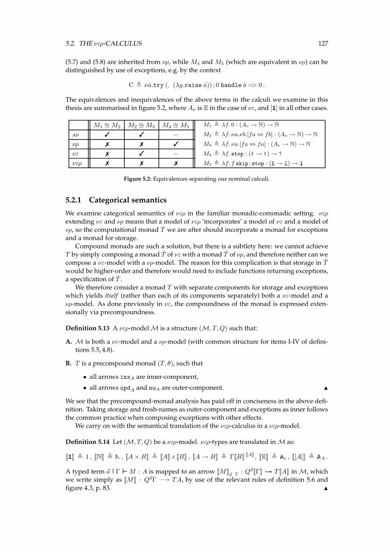
5.2. THE νερ-CALCULUS 127
(5.7) and (5.8) are inherited from νρ, while M4 and M5 (which are equivalent in νρ) can bedistinguished by use of exceptions, e.g. by the context
C , νa.try ( (λy.raise a)) ; 0 handle a => 0 .
The equivalences and inequivalences of the above terms in the calculi we examine in this
thesis are summarised in figure 5.2, where Aν is E in the case of νε, and [1] in all other cases.
M1 ≅ M2 M2 ≅ M3 M4 ≅ M5 M1 , λf. 0 : (Aν → N) → N
M2 , λf. νa.νb.[fa ⇔ fb] : (Aν → N) → N
M3 , λf. νa.[fa ⇔ fa] : (Aν → N) → N
M4 , λf. stop : (1 → 1) → 1M5 , λf. f skip ; stop : (1 → 1) → 1sν ✓ ✓ −
νρ ✗ ✗ ✓
νε ✗ ✓ −
νερ ✗ ✗ ✗
Figure 5.2: Equivalences separating our nominal calculi.
5.2.1 Categorical semantics
We examine categorical semantics of νερ in the familiar monadic-comonadic setting. νερ
extending νε and νρ means that a model of νερ ‘incorporates’ a model of νε and a model ofνρ, so the computational monad T we are after should incorporate a monad for exceptions
and a monad for storage.
Compound monads are such a solution, but there is a subtlety here: we cannot achieveT by simply composing a monad T of νεwith a monad T of νρ, and therefore neither canwe
compose a νε-model with a νρ-model. The reason for this complication is that storage in T
would be higher-order and therefore would need to include functions returning exceptions,a specification of T .
We therefore consider a monad T with separate components for storage and exceptionswhich yields itself (rather than each of its components separately) both a νε-model and a
νρ-model. As done previously in νε, the compoundness of the monad is expressed exten-
sionally via precompoundness.
Definition 5.13 A νερ-modelM is a structure (M, T,Q) such that:
A. M is both a νε-model and a νρ-model (with common structure for items I-IV of defini-tions 5.5, 4.8).
B. T is a precompound monad (T, θ), such that
• all arrows inxA are inner-component,
• all arrows updA and nuA are outer-component. N
We see that the precompound-monad analysis has paid off in conciseness in the above defi-
nition. Taking storage and fresh-names as outer-component and exceptions as inner follows
the common practice when composing exceptions with other effects.We carry on with the semantical translation of the νερ-calculus in a νερ-model.
Definition 5.14 Let (M, T,Q) be a νερ-model. νερ-types are translated inM as:
J1K , 1 , JNK , N , JA×BK , JAK×JBK , JA→ BK , T JBK JAK , JEK , Ae , J[A]K , AA .A typed term ~a ^ Γ_M : A is mapped to an arrow JMK~a^Γ : Q~aJΓK A T JAK in M, whichwe write simply as JMK : Q~aΓ B TA, by use of the relevant rules of definition 5.6 and
figure 4.3, p. 83. N
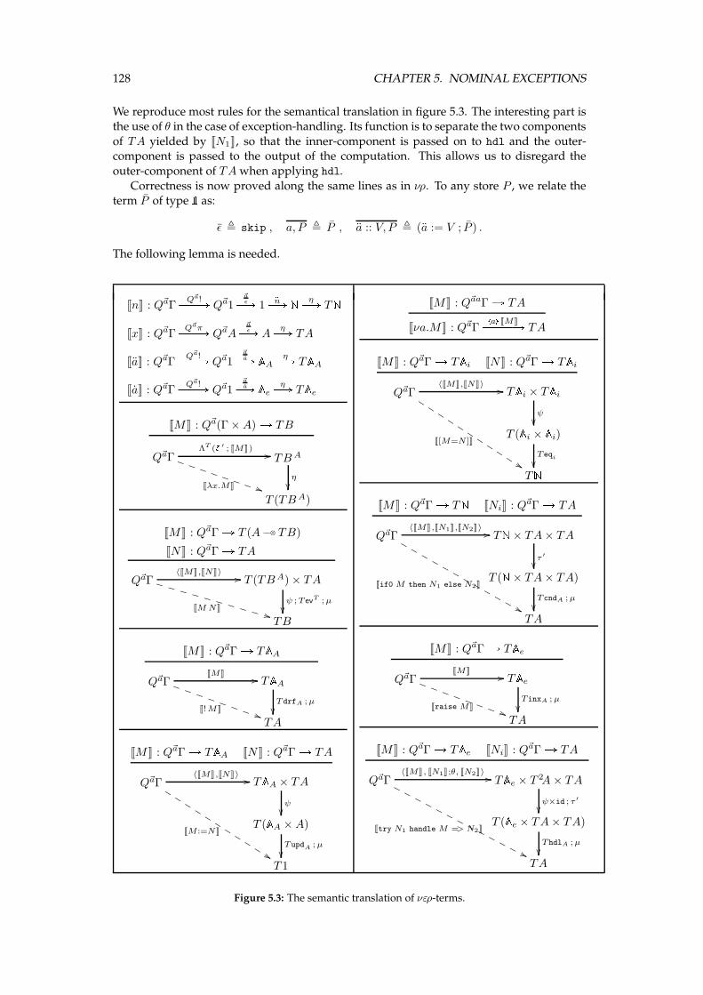
128 CHAPTER 5. NOMINAL EXCEPTIONS
We reproduce most rules for the semantical translation in figure 5.3. The interesting part isthe use of θ in the case of exception-handling. Its function is to separate the two components
of TA yielded by JN1K, so that the inner-component is passed on to hdl and the outer-component is passed to the output of the computation. This allows us to disregard the
outer-component of TAwhen applying hdl.
Correctness is now proved along the same lines as in νρ. To any store P , we relate theterm P of type 1 as:
ǫ , skip , a, P , P , a :: V, P , (a := V ; P ) .
The following lemma is needed.
JnK : Q~aΓQ~a!PPPA Q~a1
~aǫPA 1
bnPA N ηPA TN
JxK : Q~aΓQ~aπPPPA Q~aA
~aǫPA A
ηPA TA
JaK : Q~aΓQ~a!PPPA Q~a1
~aaPA AA ηPA TAA
JaK : Q~aΓQ~a!PPPA Q~a1
~aaPA Ae ηPA TAe
JMK : Q~a(Γ ×A) A TB
Q~aΓ
Jλx.MK ))TTTTTTTT
ΛT (z ′ ; JMK) // TB A
η
��T (TBA)
JMK : Q~aΓA T (A −−⊗ TB)
JNK : Q~aΓA TA
Q~aΓ
JMNK**VVVVVVVVVV
〈JMK,JNK〉 // T (TBA) × TA
ψ ;T evT ;µ
��TB
JMK : Q~aΓ A TAAQ~aΓ
J!MK))TTTTTTTT
JMK // TAATdrfA ;µ
��TA
JMK : Q~aΓA TAA JNK : Q~aΓ A TA
Q~aΓ
JM :=NK
%%KK
KK
KK
KK
KK
K
〈JMK,JNK〉 // TAA × TA
ψ��
T (AA ×A)
TupdA ; µ
��T 1
JMK : Q~aaΓ A TA
Jνa.MK : Q~aΓ\a℄ JMKPPPPPA TA
JMK : Q~aΓ A TAi JNK : Q~aΓ A TAiQ~aΓ
J[M=N ]K
%%JJ
JJ
JJ
JJ
JJ
J
〈JMK,JNK〉 // TAi × TAiψ��
T (Ai × Ai)Teqi
��TN
JMK : Q~aΓ A TN JNiK : Q~aΓ A TA
Q~aΓ
Jif0 M then N1 else N2K
&&MM
MM
MM
MM
MM
MM
〈JMK,JN1K,JN2K〉 // TN× TA× TA
τ ′
��T (N× TA× TA)
TcndA ;µ
��TA
JMK : Q~aΓ A TAeQ~aΓ
Jraise MK ))SSSSSSSS
JMK // TAeTinxA ; µ
��TA
JMK : Q~aΓ A TAe JNiK : Q~aΓ A TA
Q~aΓ
Jtry N1 handle M => N2K
''NN
NN
NN
NN
NN
NN
N
〈JMK, JN1K;θ, JN2K〉 // TAe × T 2A× TA
ψ×id ; τ ′
��T (Ae × TA× TA)
ThdlA ;µ
��TA
Figure 5.3: The semantic translation of νερ-terms.
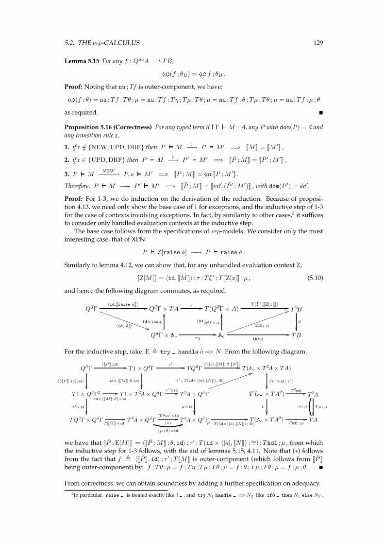
5.2. THE νερ-CALCULUS 129
Lemma 5.15 For any f : Q~aaAB TB,\a℄(f ; θB) = \a℄ f ; θB .
Proof: Noting that nu ;Tf is outer-component, we have:\a℄(f ; θ) = nu ;Tf ;Tθ ;µ = nu ;Tf ;Tη ;Tµ ;Tθ ;µ = nu ;Tf ; θ ;Tµ ;Tθ ;µ = nu ;Tf ;µ ; θ
as required. �
Proposition 5.16 (Correctness) For any typed term ~a ^ Γ_M : A, any P with dom(P ) = ~a and
any transition rule r,
1. if r /∈ {NEW,UPD,DRF} then P `Mr
−−→ P `M ′ =⇒ JMK = JM ′K ,
2. if r ∈ {UPD,DRF} then P `Mr
−−→ P ′ `M ′ =⇒ JP ;MK = JP ′ ;M ′K ,
3. P `MNEW
−−−−−→ P, a`M ′ =⇒ JP ;MK = \a℄ JP ;M ′K .
Therefore, P `M −→→ P ′ `M ′ =⇒ JP ;MK = Jν~a′.(P ′ ;M ′)K , with dom(P ′) = ~a~a′.
Proof: For 1-3, we do induction on the derivation of the reduction. Because of proposi-
tion 4.13, we need only show the base case of 1 for exceptions, and the inductive step of 1-3
for the case of contexts involving exceptions. In fact, by similarity to other cases,2 it sufficesto consider only handled evaluation contexts at the inductive step.
The base case follows from the specifications of νερ-models. We consider only the mostinteresting case, that of XPN:
P ` Z[raise a] −−→ P ` raise a .
Similarly to lemma 4.12, we can show that, for any unhandled evaluation context Z,
JZ[M ]K = 〈id, JMK〉 ; τ ;T ζ ′ ;T JZ[x]K ;µ , (5.10)
and hence the following diagram commutes, as required.
Q~aΓ
〈id,|a|〉 ))SSSSSSSSSSSSSSSSS
〈id,Jraise aK〉 // Q~aΓ × TAτ // T (Q~aΓ ×A)
T (z ′;JZ[x]K) // T 2B
µ
��Q~aΓ × Ae π2
//
id×inxA
OO AeinxQ~aΓ×A
OO
inxT B
55jjjjjjjjjjjjjjjjjjjjj
inxB
// TB
For the inductive step, take E , try handle a => N . From the following diagram,
Q~aΓ〈JP K,id〉 //
〈〈JP K,id〉,id〉
��
T1 × Q~aΓτ ′ //
id×〈JMK;θ,id〉
��
TQ~aΓT〈|a|,JMK;θ,JNK〉// T (Ae × T 2A × TA)
T (τ×id ; τ ′)
��T1 × Q~aΓ2
τ ′×id
��
id×(JMK;θ)×id
// T1 × T 2A × Q~aΓτ ′×id // T 3A × Q~aΓ
µ×id
��
τ ′ ; T (id×〈|a|,JNK〉 ;∼=)
55jjjjjjjjjjjjjjj
T 2(Ae × TA2)T2hdl //
µ
��
T 3A
Tµ ;µ
��µ ; µ
��TQ~aΓ × Q~aΓ
TJMK×id
// T 2A × Q~aΓ(Tθ;µ)×id//
(µ ; θ)×id
(∗) 44T2A × Q~aΓ
τ ′ ; T (id×〈|a|,JNK〉 ;∼=)
// T (Ae × TA2)Thdl ;µ
// TA
we have that JP ; E[M ]K = 〈JP ;MK ; θ, id〉 ; τ ′ ;T (id × 〈|a|, JNK〉 ;∼=) ;Thdl ;µ , from which
the inductive step for 1-3 follows, with the aid of lemmas 5.15, 4.11. Note that (∗) followsfrom the fact that f , 〈JP K, id〉 ; τ ′ ;T JMK is outer-component (which follows from JP K
being outer-component) by: f ;Tθ ;µ = f ;Tη ;Tµ ;Tθ ;µ = f ; θ ;Tµ ;Tθ ;µ = f ;µ ; θ . �
From correctness, we can obtain soundness by adding a further specification on adequacy.
2In particular, raise is treated exactly like ! , and try N1 handle => N2 like if0 then N1 else N2 .
130 CHAPTER 5. NOMINAL EXCEPTIONS
Definition 5.17 Let M be a νερ-model and J K the respective translation of νερ. M is ade-
quate if, for any typed term ~a ^∅_M : N, if JMK = Jν~b.P ; 0K , some P,~b, then there exists
P ′ such that ~a`M −→→ P ′ ` 0 . N
Proposition 5.18 (Equational Soundness) Translating νερ into an adequate νερ-model M weobtain:
JMK = JNK =⇒ M / N .�
5.2.2 Full abstraction
Normally we would expect to obtain full-abstraction from soundness by adding furtherspecifications to νερ-models, and perhaps doing some quotienting, but this is not the case
here. For full-abstraction the model needs to satisfy definability, at least for the arrowsdefining the semantical preorder. However, θ is clearly not definable— there is no context
separating the computational effects in the manner θ does— and its presence affects the
semantical preorder in a substantial way. For the latter, note for example that the terms
a := 0 ; raise νa.a and a := 1 ; raise νa.a
are observationally equivalent in the language, but their translations can be distinguishedby use of θ: simply discard their inner-component computations by composing them with
θ ;T !, and then return the value of a.Since it is unreasonable to ask definability with θ, we will remove it from our models and
thus work in νερ-submodels, that is, submodels of νερ-models that contain the translations of
all νερ-terms but not problematic arrows like θ.
Definition 5.19 Let M = (M, T,Q) be an adequate νερ-model and let J K be the semantic
translation of νερ into M. A νερ-submodel is a structure (M′, T ′, Q′
) such that:
• M′ is a lluf subcategory of M, and T ′, Q′
are restrictions of T,Q inM′.
• (M′, T ′, Q′
) satisfies items I-IV of definitions 5.5,4.8.
• JMK ∈ M′(Q′~aJΓK, T ′JAK), for each typed term ~a ^ Γ_M : A. N
By a slight abuse of notation, we denote M′ by (M′, T,Q). Evidently, a νερ-submodel M′
is an adequate model of νερ. Regarding observationality, since the intrinsic preorder cannot
be shown to be a congruence (the semantic translation comes from M as a black box), it is
stipulated to be so.
Definition 5.20 A νερ-submodel M′ = (M′, T,Q) is observational if:
• for all ~a, there exists O~a ⊆ M′(Q~a1, TN) such that, for all ~a ^∅_M :N,
JMK∈O~a ⇐⇒ ∃P,~b. JMK = Jν~b.P ; 0K ,
• the induced intrinsic preorder .= (.~a)~a∈A# , defined on arrows inM′(Q~aA, TB) by
f .~a g ⇐⇒ ∀ρ : Q~a(TB A)B TN. (Λ~a(f) ; ρ ∈ O~a =⇒ Λ~a(g) ; ρ ∈ O~a) ,
with Λ~a(f) , ΛQ~a,T (f), is a congruence.
We write M′ as (M′, T,Q,O). N
Recall from definition 4.17 that. being a congruence means that, for any pairM,N of terms
and any relevant context C,
JMK . JNK =⇒ JC[M ]K . JC[N ]K .
We can now prove the following.
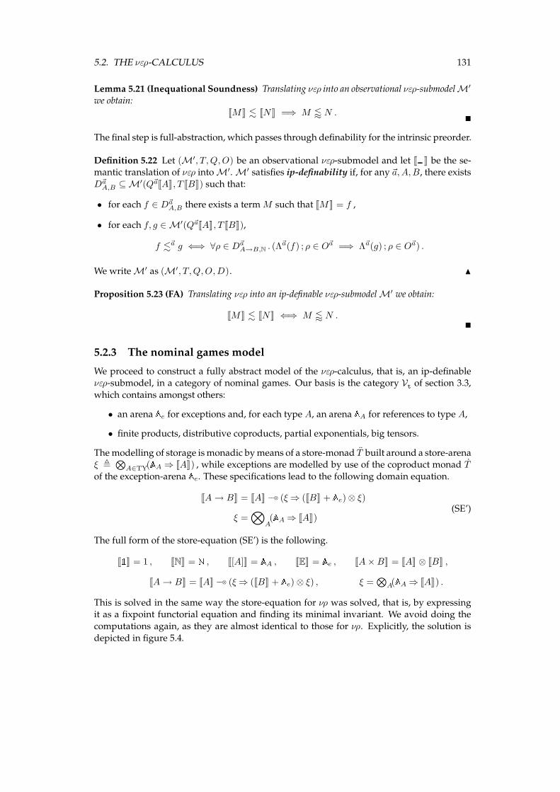
5.2. THE νερ-CALCULUS 131
Lemma 5.21 (Inequational Soundness) Translating νερ into an observational νερ-submodelM′
we obtain:
JMK . JNK =⇒ M / N .�
The final step is full-abstraction, which passes through definability for the intrinsic preorder.
Definition 5.22 Let (M′, T,Q,O) be an observational νερ-submodel and let J K be the se-mantic translation of νερ intoM′. M′ satisfies ip-definability if, for any ~a,A,B, there exists
D~aA,B ⊆ M′(Q~aJAK, T JBK) such that:
• for each f ∈ D~aA,B there exists a termM such that JMK = f ,
• for each f, g ∈ M′(Q~aJAK, T JBK),
f .~a g ⇐⇒ ∀ρ ∈ D~aA→B,N . (Λ~a(f) ; ρ ∈ O~a =⇒ Λ~a(g) ; ρ ∈ O~a) .
We write M′ as (M′, T,Q,O,D). N
Proposition 5.23 (FA) Translating νερ into an ip-definable νερ-submodelM′ we obtain:
JMK . JNK ⇐⇒ M / N .�
5.2.3 The nominal games model
We proceed to construct a fully abstract model of the νερ-calculus, that is, an ip-definableνερ-submodel, in a category of nominal games. Our basis is the category Vt of section 3.3,
which contains amongst others:
• an arena Ae for exceptions and, for each type A, an arena AA for references to type A,
• finite products, distributive coproducts, partial exponentials, big tensors.
Themodelling of storage ismonadic bymeans of a store-monad T built around a store-arenaξ ,
⊗
A∈TY(AA ⇒ JAK) , while exceptions are modelled by use of the coproduct monad T
of the exception-arena Ae. These specifications lead to the following domain equation.
JA→ BK = JAK −−⊗ (ξ⇒ (JBK + Ae) ⊗ ξ)
ξ =⊗
A(AA ⇒ JAK)
(SE’)
The full form of the store-equation (SE’) is the following.
J1K = 1 , JNK = N , J[A]K = AA , JEK = Ae , JA×BK = JAK ⊗ JBK ,
JA→ BK = JAK −−⊗ (ξ⇒ (JBK + Ae) ⊗ ξ) , ξ =⊗
A(AA ⇒ JAK) .
This is solved in the same way the store-equation for νρ was solved, that is, by expressingit as a fixpoint functorial equation and finding its minimal invariant. We avoid doing the
computations again, as they are almost identical to those for νρ. Explicitly, the solution is
depicted in figure 5.4.
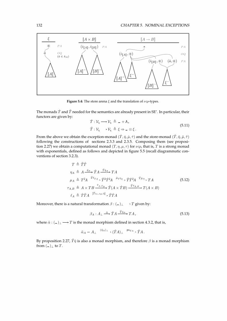
132 CHAPTER 5. NOMINAL EXCEPTIONS
ξ
⊛ PA
a OQ(a ∈ AA)
JAK
JA ×BK
(iJAK , iJBK) PA
JAK−
JBK−
JA→ BK
∗ PA
(iJAK ,⊛) OQ
JAK− ξ−
(iJBK ,⊛) (a,⊛) PA
JBK− ξ−
Figure 5.4: The store arena ξ and the translation of νερ-types.
The monads T and T needed for the semantics are already present in SE’. In particular, theirfunctors are given by:
T : Vt B Vt , + AeT : Vt B Vt , ξ⇒ ⊗ ξ .
(5.11)
From the above we obtain the exception-monad (T , η, µ, τ ) and the store-monad (T , η, µ, τ )
following the constructions of sections 2.3.3 and 2.3.5. Composing them (see proposi-
tion 2.27) we obtain a computational monad (T, η, µ, τ) for νερ, that is, T is a strong monadwith exponentials, defined as follows and depicted in figure 5.5 (recall diagrammatic con-
ventions of section 3.2.3).
T , T T
ηA , AηAPPA TA
T ηAPPPA TA
µA , T 2AT ℓTAPPPPA T 2T 2A
µT2APPPPA T T 2AT µAPPPA TA
τA,B , A× TBτA,TBPPPPA T (A× TB)
T τA,BPPPPPA T (A×B)
ℓA , T TA[T ι1, ι2; η]PPPPPPPA T TA
(5.12)
Moreover, there is a natural transformation β : ( )⊥ B T given by:
βA : A⊥αPA TA
T ηAPPPA TA , (5.13)
where α : ( )⊥ B T is the monad morphism defined in section 4.3.2, that is,
αA = A⊥(ηA)⊥PPPPPA (TA)⊥
puT APPPPA TA .
By proposition 2.27, T η is also a monad morphism, and therefore β is a monad morphism
from ( )⊥ to T .
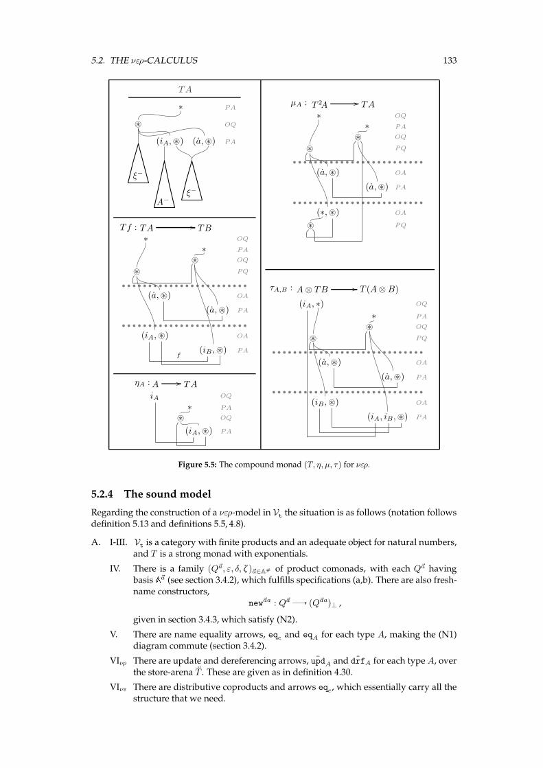
5.2. THE νερ-CALCULUS 133
TA
∗ PA
⊛ OQ
ξ−
(iA,⊛) (a,⊛) PA
A−ξ−
TATf : // TB∗ OQ
∗ PA
⊛ OQ
⊛ PQ
(a,⊛) OA
(a,⊛) PA
(iA,⊛) OA
(iB,⊛) PAf
AηA : // TAiA OQ
∗ PA
⊛ OQ
(iA,⊛) PA
T 2AµA : // TA∗ OQ
∗ PA
⊛ OQ
⊛ PQ
(a,⊛) OA
(a,⊛) PA
(∗,⊛) OA
⊛ PQ
A⊗ TBτA,B : // T (A⊗B)
(iA, ∗) OQ
∗ PA
⊛ OQ
⊛ PQ
(a,⊛) OA
(a,⊛) PA
(iB,⊛) OA
(iA, iB,⊛) PA
Figure 5.5: The compound monad (T, η, µ, τ ) for νερ.
5.2.4 The sound model
Regarding the construction of a νερ-model in Vt the situation is as follows (notation followsdefinition 5.13 and definitions 5.5, 4.8).
A. I-III. Vt is a category with finite products and an adequate object for natural numbers,
and T is a strong monad with exponentials.
IV. There is a family (Q~a, ε, δ, ζ )~a∈A# of product comonads, with each Q~a havingbasis A~a (see section 3.4.2), which fulfills specifications (a,b). There are also fresh-
name constructors,new~aa : Q~aB (Q~aa)⊥ ,
given in section 3.4.3, which satisfy (N2).
V. There are name equality arrows, eqe and eqA for each type A, making the (N1)diagram commute (section 3.4.2).
VIνρ There are update and dereferencing arrows, ¨updA and ¨drfA for each type A, over
the store-arena T . These are given as in definition 4.30.
VIνε There are distributive coproducts and arrows eqe, which essentially carry all the
structure that we need.
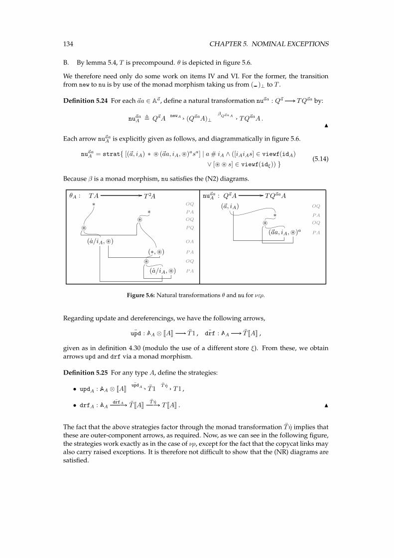
134 CHAPTER 5. NOMINAL EXCEPTIONS
B. By lemma 5.4, T is precompound. θ is depicted in figure 5.6.
We therefore need only do some work on items IV and VI. For the former, the transitionfrom new to nu is by use of the monad morphism taking us from ( )⊥ to T .
Definition 5.24 For each ~aa ∈ A~a, define a natural transformation nu~aa : Q~aB TQ~aa by:
nu~aaA , Q~aAnewAPPPA (Q~aaA)⊥
βQ~aaAPPPPPA TQ~aaA .
N
Each arrow nu~aaA is explicitly given as follows, and diagrammatically in figure 5.6.
nu~aaA = strat{ [(~a, iA) ∗ ⊛ (~aa, iA,⊛)asa] | a# iA ∧ ([iAiAs] ∈ viewf(idA)
∨ [⊛ ⊛ s] ∈ viewf(idξ)) }(5.14)
Because β is a monad morphism, nu satisfies the (N2) diagrams.
TAθA : // T 2A∗ OQ
∗ PA
⊛ OQ
⊛ PQ
(a/iA,⊛) OA
(∗,⊛) PA
⊛ OQ
(a/iA,⊛) PA
Q~aAnu~aaA : // TQ~aaA
(~a, iA) OQ
∗ PA
⊛ OQ
(~aa, iA,⊛)a PA
Figure 5.6: Natural transformations θ and nu for νερ.
Regarding update and dereferencings, we have the following arrows,
¨upd : AA ⊗ JAK B T1 , ¨drf : AA B T JAK ,
given as in definition 4.30 (modulo the use of a different store ξ). From these, we obtain
arrows upd and drf via a monad morphism.
Definition 5.25 For any type A, define the strategies:
• updA : AA ⊗ JAK¨updAPPPA T1
T ηPPA T 1 ,
• drfA : AA ¨drfAPPPA T JAKT ηPPA T JAK . N
The fact that the above strategies factor through the monad transformation T η implies thatthese are outer-component arrows, as required. Now, as we can see in the following figure,
the strategies work exactly as in the case of νρ, except for the fact that the copycat links mayalso carry raised exceptions. It is therefore not difficult to show that the (NR) diagrams are
satisfied.
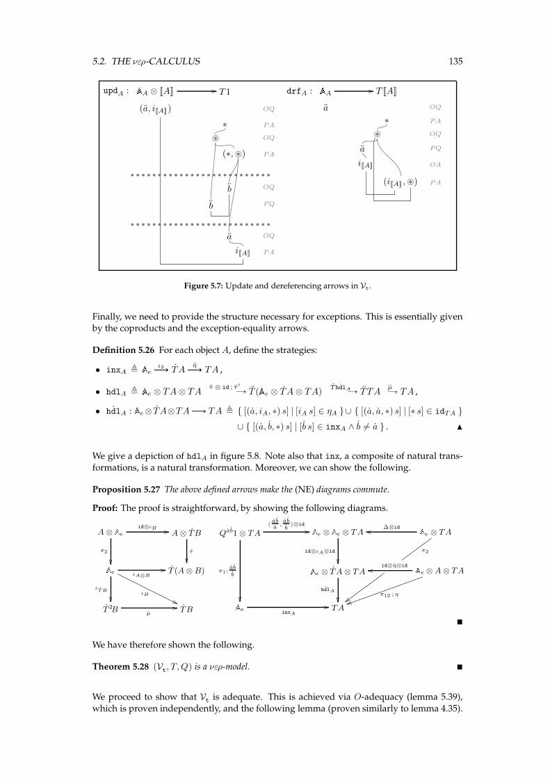
5.2. THE νερ-CALCULUS 135AA ⊗ JAKupdA : // T 1
(a, iJAK) OQ
∗ PA
⊛ OQ
(∗,⊛) PA
b OQ
b PQ
a OQ
iJAK PA
AAdrfA : // T JAK
a OQ
∗ PA
⊛ OQ
a PQ
iJAK OA
(iJAK ,⊛) PA
Figure 5.7: Update and dereferencing arrows in Vt.
Finally, we need to provide the structure necessary for exceptions. This is essentially givenby the coproducts and the exception-equality arrows.
Definition 5.26 For each object A, define the strategies:
• inxA , Ae ι2PA TAηPA TA ,
• hdlA , Ae ⊗ TA⊗ TAτ ⊗ id ; τ ′PPPPPPPA T (Ae ⊗ TA⊗ TA)
T ˙hdlAPPPPPA T TAµPA TA ,
• ˙hdlA : Ae⊗ TA⊗TAB TA , { [(a, iA, ∗) s] | [iA s] ∈ ηA }∪ { [(a, a, ∗) s] | [∗ s] ∈ idTA }
∪ { [(a, b, ∗) s] | [b s] ∈ inxA ∧ b 6= a } . N
We give a depiction of hdlA in figure 5.8. Note also that inx, a composite of natural trans-
formations, is a natural transformation. Moreover, we can show the following.
Proposition 5.27 The above defined arrows make the (NE) diagrams commute.
Proof: The proof is straightforward, by showing the following diagrams.
A ⊗ Ae id⊗ιB //
π2
��
A ⊗ TB
τ
��Ae ιA⊗B
//
ιB
''OOOOOOOOOOOOOOO
ιT B
��
T (A ⊗ B)
T 2Bµ
// TB
Qab1 ⊗ TA
〈aba,ab
b〉⊗id
//
π1;ab
b
��
Ae ⊗ Ae ⊗ TA
id⊗ιA⊗id
��
Ae ⊗ TA∆⊗idoo
wwwwwwww
π2
{{wwwwwwwwww
wAe ⊗ TA ⊗ TA
˙hdlA
��
Ae ⊗ A ⊗ TAid⊗η⊗idoo
π12 ; η
uukkkkkkkkkkkkkkkkkkAeinxA
// TA
�
We have therefore shown the following.
Theorem 5.28 (Vt, T,Q) is a νερ-model. �
We proceed to show that Vt is adequate. This is achieved via O-adequacy (lemma 5.39),
which is proven independently, and the following lemma (proven similarly to lemma 4.35).
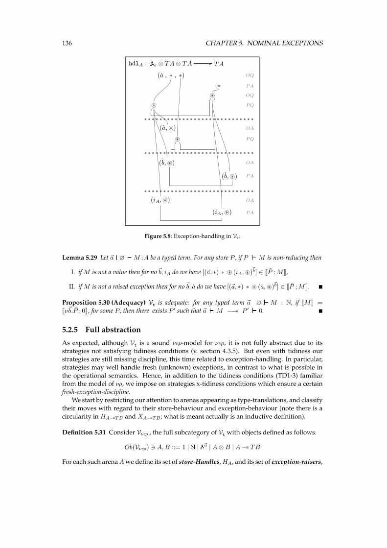
136 CHAPTER 5. NOMINAL EXCEPTIONSAe ⊗ TA⊗ TAhdlA : // TA
(a , ∗ , ∗) OQ
∗ PA
⊛ OQ
⊛ PQ
(a,⊛) OA
⊛ PQ
(b,⊛) OA
(b,⊛) PA
(iA,⊛) OA
(iA,⊛) PA
Figure 5.8: Exception-handling in Vt.
Lemma 5.29 Let ~a ^∅_M :A be a typed term. For any store P , if P `M is non-reducing then
I. ifM is not a value then for no~b, iA do we have [(~a, ∗) ∗ ⊛ (iA,⊛)~b] ∈ JP ;MK,
II. ifM is not a raised exception then for no~b, a do we have [(~a, ∗) ∗ ⊛ (a,⊛)~b] ∈ JP ;MK. �
Proposition 5.30 (Adequacy) Vt is adequate: for any typed term ~a ^∅_M : N, if JMK =
Jν~b.P ; 0K, for some P , then there exists P ′ such that ~a`M −→→ P ′ ` 0. �
5.2.5 Full abstraction
As expected, although Vt is a sound νερ-model for νερ, it is not fully abstract due to its
strategies not satisfying tidiness conditions (v. section 4.3.5). But even with tidiness ourstrategies are still missing discipline, this time related to exception-handling. In particular,
strategies may well handle fresh (unknown) exceptions, in contrast to what is possible in
the operational semantics. Hence, in addition to the tidiness conditions (TD1-3) familiarfrom the model of νρ, we impose on strategies x-tidiness conditions which ensure a certain
fresh-exception-discipline.We start by restricting our attention to arenas appearing as type-translations, and classify
their moves with regard to their store-behaviour and exception-behaviour (note there is a
circularity inHA−−⊗TB and XA−−⊗TB ; what is meant actually is an inductive definition).
Definition 5.31 Consider Vνερ , the full subcategory of Vt with objects defined as follows.
Ob(Vνερ) ∋ A,B ::= 1 | N | A~a | A⊗B | A −−⊗ TB
For each such arenaAwe define its set of store-Handles,HA, and its set of exception-raisers,

5.2. THE νερ-CALCULUS 137
XA, as follows.
H1 =HN = HA~a , ∅ ,
HA⊗B ,HA ∪HB ,
HA−−⊗TB , {(iA,⊛A), (iB,⊛B), (a,⊛B)} ∪HA ∪HB ∪HξA∪HξB
, withHξ ,⋃
C HJCK ;
X1 =XN = XA~a , ∅ ,
XA⊗B ,XA ∪XB ,
XA−−⊗TB , {(a,⊛B)} ∪XA ∪XB ∪XξA∪XξB
, with Xξ ,⋃
C XJCK ;
where we write A −−⊗ TB as A −−⊗ (ξA ⇒ (B + Ae) ⊗ ξB), and ξ as⊗
C(AC ⇒ JCK).In an arena A, a store-Handle justifies (all) Questions of the form a, which we call store-
Questions. Answers to store-Questions are called store-Answers. N
The classification of moves relatively to the store is familiar from νρ. Regarding exceptions,it is obvious that X-raisers are moves that raise an exception—note here that exception
names may also appear in a play as values (i.e. not inside X-raisers). We observe that X-
raisers are by definition A-store-H’s, justified by Q-store-H’s, and that every Q-store-H jus-tifies X-raisers. An example of how the above classes of moves are related is given in the
next figure.
ξ⇒ (1 + AE) ⊗ ξ
∗
⋄ ⊛
⊲ a ⋄ (∗,⊛) ⋄ (a,⊛) z
⊳ iA ⊲ b ⊲ c
⊳ iB ⊳ iC
store-H’s: ⋄ store-Q’s: ⊲
store-A’s: ⊳ X-raisers: z
Figure 5.9: Store-H’s -Q’s -A’s and X-raisers in arena T1.
From now on we work in Vνερ , unless stated otherwise. The above notions can be straight-forwardly extended to prearenas, by setting
HA→B , HA ∪HB , XA→B , XA ∪XB , (5.15)
and similarly for store-Q’s and store-A’s. As in section 4.3.5, we can show that a move isexclusively either initial or a store-H or a store-Q or a store-A.
Proposition 5.32 For any type A ∈ Ob(Vνερ),
MA = IA ⊎HA ⊎ {m ∈MA |m a store-Q} ⊎ {m ∈MA |m a store-A} .�
Around these notions we define x-tidy strategies. Note that we endorse again the following
notational convention. Since stores ξmay occur in several places inside a (pre)arenawemayuse parenthesised indices to distinguish identical moves from different stores. For example,
the same store-question q may be occasionally denoted q(O) or q(P ) , the particular notationdenoting the OP-polarity of the moves.
138 CHAPTER 5. NOMINAL EXCEPTIONS
Definition 5.33 A total strategy σ is x-tidy if whenever odd-length [s] ∈ σ then:
(TD1) If s ends in a store-Q q then [sx] ∈ σ , with x being either a store-A to q introducingno new names, or a copy of q. In particular, if q = a~a with a # psq− then the latter
case holds.
(TD2) If [sq(P )] ∈ σ with q a store-Q then q(P ) is justified by the last O-store-H in psq.
(TD3) If psq = s′q(O)q(P )t y(O) with q a store-Q then [s y(P )] ∈ σ with y(P) justified by psq .−3 .
(xTD1) If s ends in an X-raiser (a,⊛)~a with a# psq− then [s(a,⊛)~a] ∈ σ.
(xTD3) If psq = s′(a,⊛)~a(O)(a,⊛)~a(P )q(O) with q a store-Q, (a,⊛)(O) an X-raiser and a# s′, then[s q(P )] ∈ σ. N
The (TD) conditions define tidy strategies as in section 4.3.5, imposing thus a certain store-
discipline. The (xTD) conditions provide a fresh-exception-discipline:
When a fresh raised exception is encountered, it is simply copycatted.
In (xTD1), the X-raiser (a,⊛)~a played by Player is an answer and hence needs to be justified
by the pending question; the following lemma shows that this is always possible.
Lemma 5.34 If odd-length [s] ∈ σ ends in an X-raiser (a,⊛)~a then s has a pending-Q which is an
O-store-H, and s(a,⊛)~a is a play.
Proof: s being odd-length implies that it has a pending question, say q. If q were a P-movethen s = s1qs2 with s1, s2 being odd-length, so anA in s2 should be justified by q,. Hence,
q an O-move. Moreover, q cannot be initial, by totality, and neither a store-Q: q being unan-swered would mean that P copycats after it, so the move following q would be a copy of
it answered by an O-store-A y, say. After y is played, P must answer q with a copy of y,
thus y can only be the last move in s, i.e. (a,⊛)~a, as y a store-A. Hence, q an O-store-H.Thus, s(a,⊛)~a is a justified sequence satisfying well-bracketing, and it clearly satisfies NC’s.
Finally, it also satisfies visibility since s and psq have the same pending-Q (see e.g. [McC98]).�
It is easy to see that identity arrows are x-tidy. Moreover, x-tidy strategies compose and thuswe have a category of nominal arenas and x-tidy strategies.
Proposition 5.35 If σ : AB B and τ : BB C are x-tidy strategies then so is σ ; τ .
Proof: Fromproposition 4.56we know that σ ; τ satisfies the (TD) conditions. The (xTD) con-ditions are shown similarly. We only show (xTD1). So let odd-length [s ; t] ∈ σ ; τ be ending
in an X-raiser (a,⊛)~a′
with a# ps ; tq−. Assume, wlog, that s ; t ends in A, so s.−1 = (a,⊛)~a1 ,some~a1 � ~a′. Then, similarly to proposition 3.36, a#psq− so, by x-tidiness, [s(a,⊛)~a1 ] ∈ σ. If
(a,⊛)~a1 is in A then we are done. Otherwise, we have that [t(a,⊛)~a2 ] ∈ τ some ~a2 � ~a′. Ap-
plying the same reasoning consecutively, some (a,⊛)~an is played in AC, giving the requiredcopy of (a,⊛)~a
′
. �
Definition 5.36 xT is the lluf subcategory of Vνερ of x-tidy strategies. N
Many of the strategies we have encountered thus far are x-tidy, but not all of them: θA is not
x-tidy, for any object A. But this was exactly the reason for introducing νερ-submodels in
definition 5.19. Thus, we have the following.
Proposition 5.37 xT forms a νερ-submodel of Vνερ.
Proof: It is not difficult to show the following (see also proposition 4.58).
5.2. THE νερ-CALCULUS 139
⊲ If f : A → B, g : A → C are x-tidy then 〈f, g〉 is. Moreover, projections and terminalarrows are all x-tidy.
⊲ ηA, µA, τA,B are all x-tidy, and if h is x-tidy then Th is. Moreover, f : A⊗B → TC is x-tidy
iff ΛT (f) is.
⊲ εA, δA are x-tidy, and if h is x-tidy then so is Q~ah.
⊲ Successor, predecessor and numeral arrows are x-tidy.
⊲ Name-equality arrows are x-tidy. Moreover, ( ~a~a′ )A and nu~aaA are x-tidy.
⊲ updA, drfA are x-tidy.
⊲ inxA are x-tidy, and so are the following composite strategies.Ae ⊗ TA⊗ TAid ⊗ θA ⊗ idPPPPPPPPPA Ae ⊗ T 2A⊗ TA
τ ⊗ id ; τ ′PPPPPPPA T (Ae ⊗ TA⊗ TA)ThdlA ;µPPPPPPPA TA
Hence, xT is a νερ-submodel. �
Henceforth, by strategies we shall mean x-tidy strategies, unless stated otherwise.
We now proceed to add the structure necessary for an observational νερ-submodel.
Definition 5.38 Expand xT to (xT , T,Q,O) by setting, for each ~a,
O~a , {f ∈ xT (Q~a1, TN) | ∃~b. [(~a, ∗) ∗ ⊛ (0,⊛)~b] ∈ f} .
N
With the above definition, the semantic preorder is given as follows. For each f, g ∈ xT (Q~aA, TB),
f .~a g ⇐⇒ ∀ρ∈xT (Q~a(A −−⊗ TB), TN). (Λ~a(f) ; ρ ∈ O~a =⇒ Λ~a(g) ; ρ ∈ O~a) ,
where
Λ~a(f) = ΛQ~a,T (f) , Q~a1 δPA Q~aQ~a1
Q~aΛT (z ′ ; f)PPPPPPPPPA Q~a(A −−⊗ TB) .
In order to show observationality we need to show O-adequacy and that the semantical
preorder is a congruence. The former is shown in the next lemma. The latter can be shownas in the case of νρ (section 4.3.6) and lemma 4.18 (note that we do not need to consider θ
itself, but rather the x-tidy arrow of proposition 5.37 which includes it).
Lemma 5.39 (O-Adequacy) Let ~a ^∅_M : N be a typed term. If JMK ∈ O~a then there exists
some P such that ~a`M −→→ P ` 0.
Proof: By lemma 5.29 it suffices to show that, for any such M , there is a non-reducing se-quent P ` N such that ~a`M −→→ P ` N , as thenN would necessarily be 0. For sake of
contradiction suppose the opposite, that is, that there exists an infinite reduction sequence
starting from ~a`M .The sequence must contain infinitely many reductions from the set {HL,NHL,VHL,XPN},or otherwise it would end in an infinite reduction sequence in νρ, contradicting the lat-ter’s O-adequacy (lemma 4.62). Moreover, if it contained infinitely many reductions from
{NHL,XPN,VHL} but finitely many HL reductions, then it would have either to terminate
at some raised exception or to end in an infinite sequence of reductions in νρ+VHL. The lat-ter would then produce an infinite reduction sequence in νρ. We therefore have that ~a`M
has a reduction sequence containing infinitely many HL reductions.Now we can apply a similar methodology to lemma 4.62. Namely, for each termM , define
(M)[by induction as follows.
(a)[ , a , (x)[ , x , . . . (λx.M)[ , λx.(M)[ , (M N)[ , (M)[(N)[ , . . .
140 CHAPTER 5. NOMINAL EXCEPTIONS
and (try N1 handleM => N2)[ , try (N1)
[handle (M)[=> νa.(N2)[, some a /∈ fn(N2) .
We can show that J(M)[K ⋍ JMK, by induction onM .
Now, for the term M we are examining, JMK ∈ O~a implies J(M)[K ∈ O~a. Moreover, since~a ` M diverges using infinitely many HL reduction steps, ~a ` (M)[ diverges using in-
finitely many NEW reduction steps. But the latter contradicts J(M)[K ∈ O~a. �
Hence, we can show the following.
Proposition 5.40 (Observationality) xT is observational. �
Our last task is to show ip-definability. Ourmethodology follows closely that of section 4.3.7,
and therefore wewill be omitting some proofs which are similar to proofs presented therein.We start by defining truncation functions for x-tidy strategies, the notion of finitary strat-
egy, and a sub-strategy constructor.
Definition 5.41 Let σ : A B B in xT and let [s] ∈ viewf(σ) be of even length. Define
trunc(s) and trunc′(s) by induction as follows.
trunc(ǫ) = trunc′(ǫ) , ǫ
trunc(x(O)y(P )s′) ,
ǫ , if x = y are store-Q’s
ǫ , if x = y are fresh X-raisers
xy trunc(s′) , o.w.
trunc′(x(O)y(P )s′) ,
ǫ , if x = y are store-Q’s
ǫ , if x a store-Q, y a store-A and s′ = ǫ
ǫ , if x ∈ IA, y ∈ IB and s′ = ǫ
ǫ , if x = y are fresh X-raisers
xy trunc′(s′) , o.w.
Moreover, say σ is finitary if trunc(σ) is finite, where
trunc(σ) , {[trunc(s)] | [s] ∈ viewf(σ) ∧ |s| > 3} .
Finally, for any [t] ∈ σ define:
σ≤t , strat{[s] ∈ viewf(σ) | ∃ t′ ≤ t. trunc′(s) = pt′q} .N
Hence, we call finitary those strategies whose viewfunctions become finite if we delete allthe store-copycats, all default initial answers, and all fresh-exception-copycats. On the other
hand, the strategy σ≤t is the strategy we are left with if we truncate viewf(σ) by removing
all its branches of length greater than 3 which are not contained in t, except for:
• the store-copycats and the fresh-exception-copycats, which are left intact,
• the store-A’s branches which are truncated to the point of leaving solely the store-A,so that we retain tidiness.
Note that, in general, trunc′(s) ≤ trunc(s) ≤ s. We can now show the following.
Proposition 5.42 If σ is an x-tidy strategy and [t] ∈ σ is even-length then σ≤t is a finitary x-tidystrategy with [t] ∈ σ≤t and σ≤t ⊑ σ. �
The proof of definability is facilitated by the following decomposition lemma (cf. lemma 4.66
and its proof).
5.2. THE νερ-CALCULUS 141
Lemma 5.43 (Decomposition Lemma) Let σ : Q~aJAK B T JBK be a strategy. We can decom-pose σ as follows.
1. If there exists an iA(0) such that ∃x0. [(~a, iA(0)) ∗ ⊛ x0] ∈ σ then
σ = Q~aJAK〈[x
~a= iA(0)], 〈σ0, σ
′〉〉PPPPPPPPPPPPPPPA N⊗ (T JBK)2cndPPA T JBK
where:
[x~a= iA(0)] : Q~aJAK B N , {[(~a, iA(0)) 0]} ∪ {[(~a, iA) 1] | [(~a, iA)] 6= [(~a, iA(0))]} ,
σ0 : Q~aJAK B T JBK , strat{ [(~a, iA(0)) s] ∈ viewf(σ) } ,
σ′ : Q~aJAK B T JBK , strat{ [(~a, iA) s] ∈ viewf(σ) | [(~a, iA)] 6= [(~a, iA(0))] } .
2. If there exists an iA(0) such that ∀iA. (∃x0. [(~a, iA) ∗ ⊛ x0] ∈ σ) ⇐⇒ [(~a, iA)] = [(~a, iA(0))] ,
then σ = \~b℄σ~b , where:σ~b : Q~a
~bJAK B T JBK , strat{ [(~a~b, iA(0))∗⊛m0 sr~b] | [(~a, iA(0)) ∗⊛m
~b0 s] ∈ viewf(σ) } .
3. If there exist iA(0),m0 such that ∀iA, x. [(~a, iA) ∗ ⊛ x] ∈ σ ⇐⇒ [(~a, iA)x] = [(~a, iA(0))m0] ,
then one of the following is the case.
(a) m0 = a, a store-Q of type C under ⊛, in which case we have σ = σ′ ↾ (~a, iA(0)), where:
σ′ , Q~aJAK〈id, φ〉PPPPA Q~aJAK ⊗ T JCK
τ ;Tz ′PPPPPA TQ~a(JAK ⊗ JCK)TσaPPPA T 2JBK
µPA T JBK ,
σa , strat{ [(~a, iA(0), iC) ∗ ⊛ s] | [(~a, iA(0)) ∗ ⊛ a iC s] ∈ viewf(σ) } ,
φ : Q~aJAK B T JCK ,
{
Q~a! ; ~aa ; drfC , if a ∈ S(~a)
Q~aπj ; ~aǫ ; drfC , if a# ~a .
(b) m0 = jA ∨m0 = (iB/a,⊛) , a store-H, in which case if [(~a, iA(0)) ∗ ⊛m0 a iC ] ∈ σ, for
some store-Q a and store-A iC , then
σ = Q~aJAK〈∆, σa〉PPPPPA Q~aJAK ⊗Q~aJAK ⊗ T JCK
τ ;T (id⊗φ; τ);µPPPPPPPPPPPA TQ~aJAKTσ′ ;µPPPPPA T JBK
where:
σa : Q~aJAK B T JCK , strat{ [(~a, iA(0)) ∗ ⊛ (iC ,⊛) s] | [(~a, iA(0)) ∗ ⊛m0 a iC s] ∈ viewf(σ)
∨ [⊛ ⊛ s] ∈ viewf(idξ) } ,
σ′ : Q~aJAK B T JBK , strat( {[(~a, iA(0)) ∗ ⊛m0 y s] ∈ viewf(σ) | y 6= a }
∪ {[(~a, iA(0)) ∗ ⊛m0 a s] | [⊛ ⊛ a s] ∈ viewf(idξ)} ) ,
φ : Q~aJAK ⊗ JCK B T 1 ,
{
(Q~a! ; ~aa ) ⊗ idJCK ; updC , if a ∈ S(~a)
(Q~aπj ; ~aǫ ) ⊗ idJCK ; updC , if a# ~a .
In both cases above, we take j = min{j | (iA(0))j = a}. �
Theorem 5.44 (Definability) Let A,B be types and σ : Q~aJAK B T JBK be finitary. Then σ isdefinable.
Proof: The proof follows the same route as the proof of definability in νρ (theorem 4.67). We
only show the parts where there is some extra work needed.
The proof is by induction on (|trunc(σ)|, ‖σ‖). Using the Decomposition Lemma, wereduce the inductive step to showing that for any σ0 : Q~aJAK B T JBK with (0, 0) <
(|trunc(σ0)|, ‖σ0‖) ≤ (|trunc(σ)|, ‖σ‖) and such that, for some iA(0),m0,
∀iA, x. [(~a, iA) ∗ ⊛ x] ∈ σ0 ⇐⇒ [(~a, iA)x] = [(~a, iA(0))m0] ,
142 CHAPTER 5. NOMINAL EXCEPTIONS
with m0 a store-H and with σ0 not updating any names before playing m0, there exists aterm M0 with σ0 = JM0K ↾ (~a, iA(0)). The case of m0 = (iB,⊛) is treated exactly as in
theorem 4.67. We need also check the casesm0 = (a,⊛) andm0 = jA.Ifm0 = (a,⊛) then σ0 = JM0K ↾ (~a, iA(0)) by taking
M0 ,
{
raise a , if a ∈ S(~a)
raise z′j , if a# ~a ∧ j = min{i | a = (iA(0))k+i} .
If m0 = jA , played in some Ak+k′+i = A′i → A′′
i , then m0 = (iA′i,⊛) . Assume that
A′i = A′
i,1 × · · · × A′i,ni
with A′i,p’s being non-products. Now, O can either ask some name
a (which would lead to a store-CC), or answer at A′′i , or raise a known exception b, or raise
some fresh exception a (whichwould lead to an exception-CC), or play at someA′i,p of arrow
type, say A′i,p = Ci,p → C′
i,p . Hence, taking S , S(~a, iA(0)) we have:
viewf(σ0) = fA ∪⋃
b∈Sfb ∪
⋃ni
p=1fp
where:
fA , f0 ∪ { [(~a, iA(0)) ∗ ⊛ (iA′i,⊛) (iA′′
i,⊛) s] ∈ viewf(σ0) }
fb , f0 ∪ { [(~a, iA(0)) ∗ ⊛ (iA′i,⊛) (b,⊛) s] ∈ viewf(σ0) }
fp , f0 ∪ { [(~a, iA(0)) ∗ ⊛ (iA′i,⊛) (iCi,p
,⊛) s] ∈ viewf(σ0) }
f0 , { [(~a, iA(0)) ∗ ⊛ (iA′i,⊛) s] | [⊛ ⊛ s] ∈ viewf(idξ)
∨ (s.1 = (a,⊛) ∧ a /∈ S ∧ [s] ∈ viewf(idAe⊗ξ)) }
and where we assume fp , f0 if A′i,p is not an arrow type. It is not difficult to see that
fA , fb , fp are viewfunctions. Now, from fA we obtain f ′A : Q~a(JAK ⊗ JA′′
i K)B T JBK by:
f ′A , { [(~a, iA(0), iA′′
i) ∗ ⊛ s] | [(~a, iA(0)) ∗ ⊛ (iA′
i,⊛) (iA′′
i,⊛) s] ∈ fA } .
It is not difficult to see that f ′A is indeed an (x-tidy) viewfunction. By IH, there exists some
~a ^ Γ, y :A′′i _MA : B such that JMAK = strat(f ′
A).From each fp 6= f0 we obtain a viewfunction f ′
p : Q~a(JAK ⊗ JCi,pK)B T JC′i,pK by:
f ′p , {[(~a, iA(0), iCi,p
) ∗ ⊛ s] | [(~a, iA(0)) ∗ ⊛ (iA′i,⊛) (iCi,p
,⊛) s] ∈ fp} .
By IH, there exists some ~a ^ Γ, y′ : Ci,p_Mp : C′i,p such that JMpK = strat(f ′
p) , so take
Vp , λy′.Mp. For each A′i,p of non-arrow type, the behaviour of σ0 at A
′i,p is fully described
by (iA′i)p , so we take Vp to be the denotation of (iA′
i)p . 〈V1, ..., Vni
〉 is now of type A′i and
describes σ0’s behaviour in A′i.
Finally, from each fb we obtain a viewfunction:
f ′b
: Q~aJAK B T JBK , {[(~a, iA(0)) ∗ ⊛ s] | [(~a, iA(0)) ∗ ⊛ (iA′i,⊛) (b,⊛) s] ∈ fb} .
By IH, there exists some ~a ^ Γ_Mb : B such that JMbK = strat(f ′b) .
Now, taking for each known exception-name b
Nb ,
{
b , if b ∈ S(~a)
z′j , if b# ~a ∧ j = min{i | b = (iA(0))k+i} ,
and
M0 , (try (λx′.λx.(λy.MA)x′)(z′′i 〈V1, ..., Vni〉) handle
−→Nb =>
−−−−→λx.Mb) skip ,
for some x, x′ not free inMA,Mb’s, we obtain σ0 = JM0K ↾ (~a, iA(0)) . �
5.2. THE νερ-CALCULUS 143
Corollary 5.45 (ip-Definability) xT = (xT , T,Q,O) is an ip-definable νερ-submodel.
Proof: For each~a,A,B, defineD~aA,B , {f : Q~aJAK B T JBK | f is finitary} . By definability,
every f ∈ D~aA,B is definable. We need also show:
(∀ρ ∈ D~aA→B,N . Λ~a(f) ; ρ ∈ O~a =⇒ Λ~a(g) ; ρ ∈ O~a) =⇒ f .~a g .
Assume the LHS assertion holds and let Λ~a(f) ; ρ ∈ O~a, some ρ : Q~a(JAK −−⊗ T JBK) B TN.Then, let [s ; t] = [(~a, ∗) ∗ ⊛ (0,⊛)
~b] ∈ Λ~a(f) ; ρ , [s] ∈ Λ~a(f) and [t] ∈ ρ. Then, by proposi-
tion 5.42, [t] ∈ ρ≤t , so Λ~a(f) ; ρ≤t ∈ O~a. Moreover, ρ≤t ∈ D~aA→B,N , so Λ~a(g) ; ρ≤t ∈ O~a, by
hypothesis. Finally, ρ≤t ⊑ ρ implies Λ~a(g) ; ρ≤t ⊑ Λ~a(g) ; ρ , hence the latter observable, sof .~a g. �
Hence, we have finally shown the following.
Theorem 5.46 xT = (xT , T,Q,O) is a fully abstract model of νερ. �
5.2.6 Equivalences established semantically
Reasoning as in section 4.3.8 we can show that, for any B ∈ TY and taking a ∈ AB , we
have νa. ! a ≅ stopB in the νερ-calculus. Moreover, using the fact that νερ-environments are
x-tidy we can also show in a similar way that
stopB ≅ νa.raise a . (5.16)
This implies that νa.raise a / M for any ǫ ^∅_M : B, in νερ and in νε.
Let us now prove equivalence (5.3) in the νε-calculus using the full-abstraction result for
νερ. Recall that
M2 , λf. νa.νb. [fa⇔ f b] : (E → N) → N , M3 , λf.νa. [fa⇔ fa] : (E → N) → N ,
and that we need to show M2 ≅ M3 . By full-abstraction of νερ (in fact, by correctness andadequacy), it suffices to show that, for any ρ : T ((Ae −−⊗ TN) −−⊗ N) B TN which is tl4 and
does not use the store,
JM2K ; ρ ∈ Oǫ ⇐⇒ JM3K ; ρ ∈ Oǫ. (5.17)
In fact, it suffices to assume ρ does not use the store for dereferencings, i.e. it does not
ask store-Q’s unless in a copycat. The viewfunctions of JM2K and JM3K are given below.Note that we have omitted store-copycat links (as we won’t be using the store) and also the
exception-copycat that occurs if Opponent plays an exception under (b,⊛)ab(4)/(a,⊛)a(4) .

144 CHAPTER 5. NOMINAL EXCEPTIONS
1JM2K // T ((Ae −−⊗ TN) −−⊗ TN)
∗ OQ
∗ PA
⊛ OQ
(∗,⊛)(1) PA
(∗,⊛)(2)
OQ
(a,⊛)ab(3)
PQ
(c,⊛)ab OA
(c,⊛)ab PA
(n,⊛)ab OA
(b,⊛)ab
(4)PQ
(m,⊛)ab OA
(n⇔ m,⊛)ab PA
1JM3K // T ((Ae −−⊗ TN) −−⊗ TN)
∗ OQ
∗ PA
⊛ OQ
(∗,⊛)(1) PA
(∗,⊛)(2)
OQ
(a,⊛)a(3)
PQ
(c,⊛)a
OA
(c,⊛)a PA
(n,⊛)a
OA
(a,⊛)a(4)
PQ
(m,⊛)a
OA
(n⇔ m,⊛)a PA
We show only one direction of the equivalence; the other is shown by a similar argument.
Let [∗ ∗ ⊛ (0,⊛)~a] ∈ JM2K ; ρ, some ρ,~a with ρ being tl4 and not asking store-Q’s. Then,
the interaction witnessing this sequence starts with [∗ ∗ ∗ ⊛ ⊛~b], some ~b introduced by ρ,
to which JM2K plays (∗,⊛)~b(1). At this point, ρ can either play (0,⊛)~a or ask some (∗,⊛)
~b1(2).
In the latter case, JM2K plays (a1,⊛)~b1a1b1(3) and now ρ has three choices: either play some
(n,⊛)~b1a1b1~c, or ask again some (∗,⊛)
~b2(2), or play some exception (c,⊛)
~b1a1b1~c. In the latter
case, JM2K responds by also playing (c,⊛)~b1a1b1~c. Note that c cannot be b1 as then x-tidiness
of ρwould copycat the exception to the output giving [∗ ∗ ⊛ (c,⊛)~b1a1b1~c] ∈ JM2K ; ρ. Hence,
the interaction can be simulated (modulo b1 ) by JM3K ; ρ. At this point, ρ can play either
(∗,⊛)~b2(2) or (0,⊛)~a. In the former case, JM2K will play (a2,⊛)
~b2a2b2(3) with a1 6= a2. Up to now,
the interaction can be simulated by JM3K ; ρ, as the bi’s have not played any part.
So suppose that, after some rounds of Opponent answering to (ai,⊛)~biaibi(3) with excep-
tions or with fresh openings of (∗,⊛)~bj
(2), Opponent plays some (n,⊛)~bk ak bk~c. At this point,
JM2K plays (bk,⊛)~bkak bk~c(4) and the play continues. But now (bk,⊛)
~bkak bk~c(4) has hidden ak from
the P-view of ρ and therefore, because of innocence, the latter will play in the same way as if
(ak,⊛)~bak bk~c(4) had been played. Hence, JM3K ; ρ can simulate this appearance of bk. Using the
precisely the same argument for all appearances of bi’s, we have that JM3K ; ρ can simulate
the whole interaction.
Chapter 6
Conclusion
E quindi uscimmo a riveder le stelle.
Dante, La Divina Commedia, Inferno.
Summary
In this thesis we have examined the semantics of nominal computation, that is, of computa-
tion capable of creating fresh names, comparing them and passing them around. Followingthe work on the ν-calculus, a characteristic feature of our approach is the stipulation of
names being constants rather than variables. We find this more adequate not only for de-notational reasons (absence of ‘bad’ constructors) but also because it seems more intuitive:
names are just like integers, but can only be compared for equality.
The constants-as-names rationale allows for a simple— syntactic and denotational—modelling of names once an adequate framework for such constants has been laid down.
The chosen relevant framework is that of nominal sets, that is, sets supplied with atoms andatom-permutation technology, which provide an elegant foundational mathematical theory
for reasoning with names (by atoms). The whole discussion— of nominal computation and
its semantics—was made inside the universe of nominal sets.Our denotational models were built in game semantics, and in particular in nominal
games. The latter are stateful, call-by-value games built inside nominal sets: names appearas constants inside games, and states contain precisely the names created along a compu-
tation. We have examined names for general references and exceptions. The methodol-
ogy followed was that of establishing a basic category of games corresponding to a basicnominal calculus, and from that obtain models of the additional nominal computational
effects by means of computational monads. Thus, our models differ importantly from pre-
vious models of general references and exceptions. While in those models names were se-mantically modelled as compound objects encapsulating the structure necessary for name-
manipulation (i.e. read/write or raise/handle methods), in our models names are elemen-tary objects manipulated by computational monads. This feature allowed us to obtain fully
complete models without the need to add ‘bad’ constructors in the language.
Further directions
This thesis has taken some basic steps in the modelling of nominal computation which can
serve as a stable platform for further research on names. A first further direction is that of
characterising the nominal effect— i.e. the computational effect that arises from the use ofnames— in abstract categorical terms. Here we have pursued this task to some extent by
introducing the monadic-comonadic description of nominal computation, but it is evidentthat the description needs further investigation. We see that there aremoremonad-comonad
145
146 CHAPTER 6. CONCLUSION
connections to be revealed, which will simplify and further substantiate the presentation.The work of Schopp which examines categories with names [Sch06] seems to be particularly
helpful in this direction.A second direction, which has not been pursued here, is that of decidability of obser-
vational equivalence in nominal languages. The use of denotational methods, and game
semantics in particular, for attacking the problem has been extremely successful in the ‘non-nominal’ case, having characterised decidability of (fragments of) Idealized Algol [GM00,
Ong02, Mur03]. It would therefore be useful to ‘nominalise’ that body of work and applyit to nominal calculi. Already from [Mur03] we can deduce that nominal languages with
ground store are undecidable, and from [PS93] we know that equivalence is decidable for
programs of first-order type in the ν-calculus, but otherwise the problem remains open. Amajor challenge to be faced is that the fully abstract models we have devised lean heavily
on semantical quotientings and therefore disallow direct reasoning on strategies. To thisend, Laird’s approach to nominal games [Lai08] seems very relevant. A first step, covering
Reduced ML, has been taken in [MT09].
A third direction would be to examine nominal languages for concurrent computation.In concurrency, names may also appear in threads, channels etc, and it is therefore natural
to extend nominal games to the concurrent setting. Usually, the passage from sequentialgames to concurrent games is achieved by interleaving of sequential plays [GM04, Lai05],
an approach that could be tested in the nominal setting. It would also be interesting to
examine formal properties, such as private names and common store, of nominal concurrentlanguages. Work in this direction has so far only been conducted by Laird [Lai06].
Finally, it would be interesting to examine AJM-games [AJM00] under the lens of nomi-nal sets. A distinctive feature of AJM-games is the use of moves-with-tags inside a play in
order to distinguish between different threads of computation. Evidently, strategies need
only distinguish between different tags and be impervious to permutation of tags. We seethat tags play a role of names and seems therefore natural to use atoms as tags. This ap-
proach seems more natural than the usual naturals-as-tags and would greatly simplify the
presentation of AJM-games allowing also the nominal consideration of issues arising in Lin-ear Logic and Geometry of Interaction.
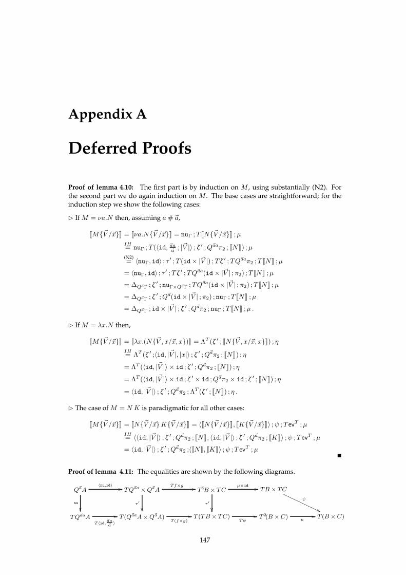
Appendix A
Deferred Proofs
Proof of lemma 4.10: The first part is by induction on M , using substantially (N2). Forthe second part we do again induction on M . The base cases are straightforward; for the
induction step we show the following cases:
⊲ IfM = νa.N then, assuming a# ~a,
JM{~V /~x}K = Jνa.N{~V /~x}K = nuΓ ;T JN{~V /~x}K ;µ
IH= nuΓ ;T (〈id, ~aa~a ; |~V |〉 ; ζ ′ ;Q~aaπ2 ; JNK) ;µ
(N2)= 〈nuΓ, id〉 ; τ ′ ;T (id× |~V |) ;T ζ ′ ;TQ~aaπ2 ;T JNK ;µ
= 〈nuΓ, id〉 ; τ ′ ;T ζ ′ ;TQ~aa(id× |~V | ;π2) ;T JNK ;µ
= ∆Q~aΓ ; ζ ′ ; nuΓ×Q~aΓ ;TQ~aa(id× |~V | ;π2) ;T JNK ;µ
= ∆Q~aΓ ; ζ ′ ;Q~a(id× |~V | ;π2) ; nuΓ ;T JNK ;µ
= ∆Q~aΓ ; id× |~V | ; ζ ′ ;Q~aπ2 ; nuΓ ;T JNK ;µ .
⊲ IfM = λx.N then,
JM{~V /~x}K = Jλx.(N{~V , x/~x, x})K = ΛT (ζ ′ ; JN{~V , x/~x, x}K) ; η
IH= ΛT (ζ ′ ;〈id, ~|V |, |x|〉 ; ζ ′ ;Q~aπ2 ; JNK) ; η
= ΛT (〈id, ~|V |〉 × id ; ζ ′ ;Q~aπ2 ; JNK) ; η
= ΛT (〈id, ~|V |〉 × id ; ζ ′ × id ;Q~aπ2 × id ; ζ ′ ; JNK) ; η
= 〈id, ~|V |〉 ; ζ ′ ;Q~aπ2 ; ΛT (ζ ′ ; JNK) ; η .
⊲ The case ofM = N K is paradigmatic for all other cases:
JM{~V /~x}K = JN{~V /~x}K{~V /~x}K = 〈JN{~V /~x}K, JK{~V /~x}K〉 ;ψ ;T evT ;µ
IH= 〈〈id, |~V |〉 ; ζ ′ ;Q~aπ2 ; JNK, 〈id, |~V |〉 ; ζ ′ ;Q~aπ2 ; JKK〉 ;ψ ;T evT ;µ
= 〈id, |~V |〉 ; ζ ′ ;Q~aπ2 ;〈JNK, JKK〉 ;ψ ;T evT ;µ�
Proof of lemma 4.11: The equalities are shown by the following diagrams.
Q~aA
nu
��
〈nu,id〉 // TQ~aa× Q~aA
τ ′
��
Tf×g // T 2B × TC
τ ′
��
µ×id // TB × TC
ψ
''PPPPPPPPPPPPP
TQ~aaAT〈id,
~aa~a
〉
// T (Q~aaA × Q~aA)T (f×g)
// T (TB × TC)Tψ
// T 2(B × C)µ
// T (B × C)
147
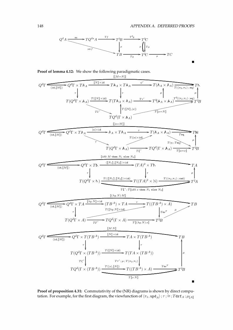
148 APPENDIX A. DEFERRED PROOFS
Q~aAnu // \a℄ f
++VVVVVVVVVVVVVVVVVVVVVVVVVV TQ~aaATf // T 2B
T2g //
µ
��
T 3C
Tµ
��µ
��TB
Tg
// T 2C µ// TC
�
Proof of lemma 4.12: We show the following paradigmatic cases.
Q~aΓ〈id,JMK〉
//
J[M=N ]K
--Q~aΓ × TAA JNK×id //
τ
��
TAA × TAA ψ′
//
τ
��
T (AA × AA)T (〈π2,π1〉 ; eq)
// TNT (Q~aΓ × AA)
T (JNK×id) //
Tz ′))SSSSSSSSSSSSSS
T (TAA × AA)Tτ ′
// T 2(AA × AA)
µ
OO
T 2(〈π2,π1〉 ; eq)// T 2B
µ
OO
TQ~a(Γ × AA)
T Jx=NK
22ffffffffffffffffffffffffffffffff
T 〈JNK,|x|〉
OO
Q~aΓ
J[a=M ]K
--〈id,JMK〉
// Q~aΓ × TAA |a|×id //
τ))SSSSSSSSSSSSSSAA × TAA τ // T (AA × AA)
Teq//
T (η ;Teq)((PPPPPPPPPPPPPPTN
T (Q~aΓ × AA)
T (|a|×id)55kkkkkkkkkkkkkk
Tz ′// TQ~a(Γ × AA)
T Ja=xK// T 2B
µ
OO
Q~aΓ
Jif0 M then N1 else N2K
--〈id,JMK〉
// Q~aΓ × TN 〈JN1K,JN2K〉×id //
τ
��
(TA)2 × TNτ
��
TA
T (Q~aΓ × N)T (〈JN1K,JN2K〉×id) //
Tz ′ ; T Jif0 x then N1 else N2K
22T ((TA)2 × N)T (〈π2,π1〉 ; cnd) // T 2A
µ
OO
Q~aΓ
J(λy.N)MK
--〈id,JMK〉
// Q~aΓ × TAJλy.NK×id //
τ
��
(TBA) × TAτ // T ((TBA) ×A)
T evT
��
TB
T (Q~aΓ ×A)
T (Jλy.NK×id)
22eeeeeeeeeeeeeeeeeeeeeeeeeeeeeee
Tz ′// TQ~a(Γ ×A)
T J(λy.N)xK// T 2B
µ
66nnnnnnnnnnnnnnn
Q~aΓ
JM NK
,,〈id,JMK〉
// Q~aΓ × T (TBA)JNK×id //
τ
��
TA× T (TBA)
τ
��
TB
T (Q~aΓ × (TB A))
Tz ′
��
T (JNK×id) // T (TA× (TB A))
Tτ ′ ;µ ; T 〈π2,π1〉
��TQ~a(Γ × (TB A))
T 〈|x|,JNK〉 //
T JxNK
22T ((TBA) ×A)T ev
T
// T 2B
µ
OO
�
Proof of proposition 4.31: Commutativity of the (NR) diagrams is shown by direct compu-
tation. For example, for the first diagram, the viewfunction of 〈π1, updA〉 ; τ ;∼= ;TdrfA ;µJAK
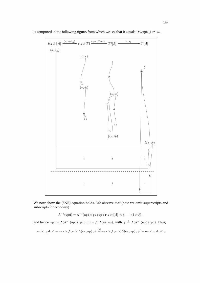
149
is computed in the following figure, from which we see that it equals 〈π2, updA〉 ; τ ;∼=.AA ⊗ JAK〈π1,updA〉 // AA ⊗ T 1
τ ;∼= ;TdrfA // T 2JAKµJAK // T JAK
(a, iA)
(a, ∗)
∗
∗
⊛
⊛
⊛
(∗,⊛)
(∗,⊛)
⊛a
a
a
iA
iA
iA
(iA,⊛)
(iA,⊛)
a
......
...
iA
b
......
...
b
We now show the (SNR) equation holds. We observe that (note we omit superscripts and
subscripts for economy)
Λ−1(upd) = Λ−1(upd) ; pu ; up : AA ⊗ JAK ⊗ ξB (1 ⊗ ξ)⊥
and hence upd = Λ(Λ−1(upd) ; pu ; up) = f ; Λ(ev ; up) , with f , Λ(Λ−1(upd) ; pu). Thus,
nu× upd ;ψ = new× f ;α× Λ(ev ; up) ;ψ(∗)= new× f ;α× Λ(ev ; up) ;ψ′ = nu× upd ;ψ′ ,
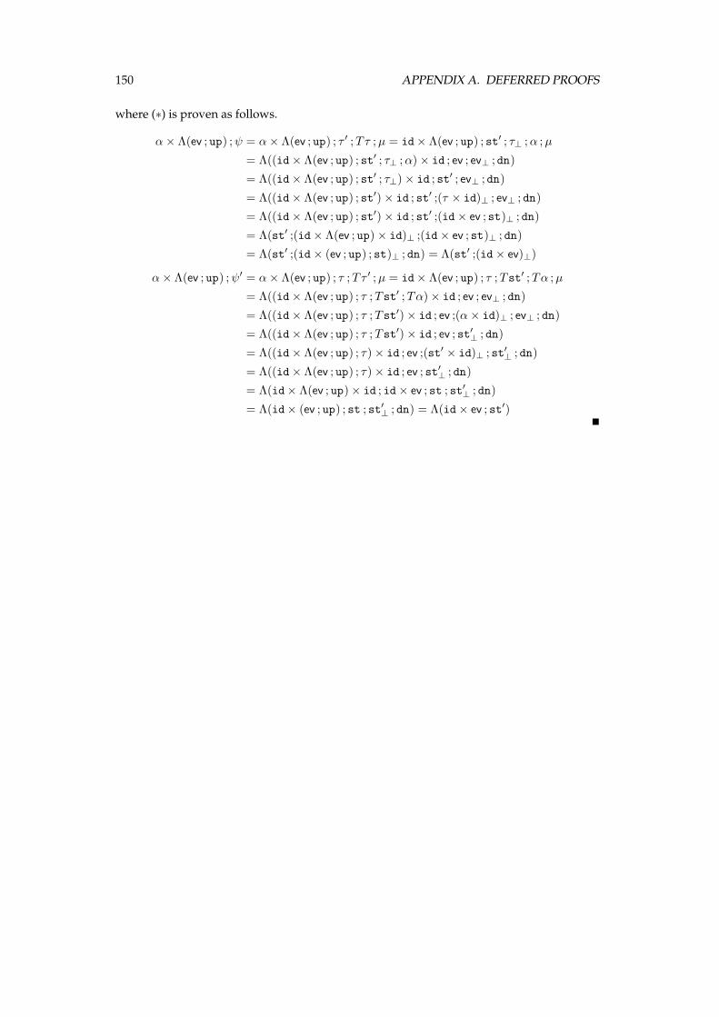
150 APPENDIX A. DEFERRED PROOFS
where (∗) is proven as follows.
α× Λ(ev ; up) ;ψ = α× Λ(ev ; up) ; τ ′ ;Tτ ;µ = id× Λ(ev ; up) ; st′ ; τ⊥ ;α ;µ
= Λ((id× Λ(ev ; up) ; st′ ; τ⊥ ;α) × id ; ev ; ev⊥ ;dn)
= Λ((id× Λ(ev ; up) ; st′ ; τ⊥) × id ; st′ ; ev⊥ ;dn)
= Λ((id× Λ(ev ; up) ; st′) × id ; st′ ;(τ × id)⊥ ; ev⊥ ; dn)
= Λ((id× Λ(ev ; up) ; st′) × id ; st′ ;(id× ev ;st)⊥ ; dn)
= Λ(st′ ;(id× Λ(ev ; up) × id)⊥ ;(id× ev ;st)⊥ ; dn)
= Λ(st′ ;(id× (ev ; up) ; st)⊥ ; dn) = Λ(st′ ;(id× ev)⊥)
α× Λ(ev ; up) ;ψ′ = α× Λ(ev ; up) ; τ ;Tτ ′ ;µ = id× Λ(ev ; up) ; τ ;Tst′ ;Tα ;µ
= Λ((id× Λ(ev ; up) ; τ ;Tst′ ;Tα) × id ; ev ; ev⊥ ; dn)
= Λ((id× Λ(ev ; up) ; τ ;Tst′) × id ; ev ;(α× id)⊥ ; ev⊥ ; dn)
= Λ((id× Λ(ev ; up) ; τ ;Tst′) × id ; ev ; st′⊥ ; dn)
= Λ((id× Λ(ev ; up) ; τ) × id ; ev ;(st′ × id)⊥ ; st′⊥ ; dn)
= Λ((id× Λ(ev ; up) ; τ) × id ; ev ; st′⊥ ; dn)
= Λ(id× Λ(ev ; up) × id ; id× ev ; st ; st′⊥ ; dn)
= Λ(id× (ev ; up) ; st ; st′⊥ ; dn) = Λ(id× ev ; st′)�

Bibliography
[Abr00] Samson Abramsky, Axioms for definability and full completeness, Proof, Language,
and Interaction: essays in honour of Robin Milner, MIT Press, 2000, pp. 55–75.
[Abr07] , Domain theory, Lecture Notes, Oxford University Computing Labora-
tory, 2007.
[AGM+04] Samson Abramsky, Dan Ghica, Andrzej Murawski, Luke Ong, and Ian Stark,Nominal games and full abstraction for the nu-calculus, LICS ’04: Proceedings of the
19th Annual IEEE Symposium on Logic in Computer Science (Turku, Finland),IEEE Computer Society Press, 2004, pp. 150–159.
[AHM98] Samson Abramsky, Kohei Honda, and Guy McCusker, A fully abstract game se-mantics for general references, LICS ’98: Proceedings of the 13th Annual IEEE Sym-
posium on Logic in Computer Science (Indianapolis, USA), IEEE Computer So-
ciety Press, 1998, pp. 334–344.
[AJ94] Samson Abramsky and Radha Jagadeesan, Games and full completeness for multi-
plicative linear logic, Journal of Symbolic Logic 59 (1994), no. 2, 543–574.
[AJM00] Samson Abramsky, Radha Jagadeesan, and Pasquale Malacaria, Full abstraction
for PCF, Information and Computation 163 (2000), no. 2, 409–470, results firstpublished in TACS ’94: Proceedings of International Symposium on Theoretical As-
pects of Computer Software (Sendai, Japan, 1994).
[AM97] Samson Abramsky and Guy McCusker, Linearity, Sharing and State: a fully ab-stract game semantics for Idealized Algol, Algol-like languages (Peter O’Hearn and
Robert D. Tennent, eds.), vol. 2, Birkhauser, 1997, 297–329, results first publishedin Proceedings of Linear Logic 96 Tokyo Meeting (Tokyo, Japan, 1996).
[AM98] , Call-by-value games, CSL ’97: Proceedings of the 11th International Work-shop on Computer Science Logic (Aarhus, Denmark), Lecture Notes in Com-
puter Science, vol. 1414, Springer-Verlag, 1998, pp. 1–17.
[AM99] , Game semantics, Computational Logic: Proceedings of the 1997 Mark-toberdorf Summer School (H. Schwichtenberg and U. Berger, eds.), Springer-
Verlag, 1999, pp. 1–56.
[Bar84] Hendrik P. Barendregt, The lambda calculus. Its syntax and semantics, Studies in
Logic and the Foundations of Mathematics, vol. 103, North-Holland, 1984.
[BDE97] Patrick Baillot, Vincent Danos, and Thomas Ehrhard, Believe it or not, AJM’s games
model is a model of classical linear logic, LICS ’97: Proceedings of the 12th Annual
IEEE Symposium on Logic in Computer Science (Warsaw, Poland), IEEE Com-puter Society Press, 1997, pp. 68–75.
[Bec69] Jon Beck, Distributive laws, Seminar on Triples and Categorical Homology The-ory, ETH, Zurich, 1966/67 (B. Eckmann, ed.), Lecture Notes in Mathematics,
vol. 80, Springer-Verlag, 1969, pp. 119–140.
151
152 BIBLIOGRAPHY
[BG92] Stephen Brookes and Shai Geva,Computational comonads and intensional semantics,Applications of Categories in Computer Science: Proceedings LMS Symposium
(Durham, UK, 1991), LondonMathematical Society Lecture Note Series, vol. 177,Cambridge University Press, 1992, pp. 1–44.
[BK08] Nick Benton and Vasileios Koutavas, Amechanized bisimulation for the nu-calculus,Tech. Report MSR-TR-2008-129,Microsoft Research, September 2008.
[BvS93] Stephen Brookes and Kathryn van Stone, Monads and comonads in intensional se-mantics, Tech. Report CMU-CS-93-140, Carnegie Mellon University, 1993.
[BW85] Michael Barr and Charles Wells, Toposes, triples and theories, Grundlehren dermathematischen Wissenschaften, vol. 278, Springer-Verlag, 1985.
[BW99] , Category theory for computing science, third ed., Les Publications CRM,
1999.
[BW02] , Toposes, triples and theories, revised version 1.1 of [BW85], available at
http://www.cwru.edu/artsci/math/wells/pub/ttt.html, November
2002.
[Che04] James Cheney,Nominal logic programming, Phd thesis, Cornell University, August
2004.
[Che05] , Nominal logic and abstract syntax, SIGACT News 36 (2005), no. 4, 47–69.
[CLW93] Aurelio Carboni, Steve Lack, and Robert Walters, Introduction to extensive and
distributive categories, Journal of Pure and Applied Algebra 84 (1993), 145–158.
[Fil99] Andrzej Filinski, Representing layered monads, POPL ’99: Proceedings of the 26th
ACM SIGPLAN-SIGACT symposium on Principles of programming languages(San Antonio, USA), ACM Press, 1999, pp. 175–188.
[Fre90] Peter J. Freyd, Recursive types reduced to inductive types, LICS ’90: Proceedings ofthe 5th Annual IEEE Symposium on Logic in Computer Science (Philadelphia,
USA), IEEE Computer Society Press, 1990, pp. 498–507.
[Gab00] Murdoch J. Gabbay, A theory of inductive definitions with α-equivalence: Seman-
tics, implementation, programming language, DPhil thesis, University of Cambridge
Computing Laboratory, 2000.
[Gab02] , FM-HOL, a higher-order theory of names, 35 Years of Automath (F. Ka-mareddine, ed.), Heriot-Watt University, Edinburgh, Scotland, April 2002.
[GM00] Dan R. Ghica andGuyMcCusker, Reasoning about Idealized Algol using regular lan-guages, ICALP ’00: Proceedings of 27th International Colloquium on Automata,
Languages and Programming (Geneva, Switzerland), LNCS, vol. 1853, Springer-
Verlag, 2000, pp. 103–116.
[GM04] Dan R. Ghica and Andrzej S. Murawski, Angelic semantics of fine-grained concur-
rency, FoSSaCS ’04: Proceedings of the 7th International Conference on Founda-tions of Software Science and Computation Structures (Barcelona, Spain), Lec-
ture Notes in Computer Science, vol. 2987, Springer, 2004, pp. 211–225.
[GP02] Murdoch J. Gabbay and Andrew M. Pitts, A new approach to abstract syntax with
variable binding, Formal Aspects of Computing 13 (2002), 341–363, results firstpublished in LICS ’99: Proceedings of the 14th Annual IEEE Symposium on Logic in
Computer Science (Trento, Italy, 1999).
[Har99] Russell Harmer, Games and full abstraction for nondeterministic languages, DPhil
thesis, University of London, 1999.
BIBLIOGRAPHY 153
[HM99] Russell Harmer and Guy McCusker, A fully abstract game semantics for finite non-determinism, LICS ’99: Proceedings of the 14thAnnual IEEE Symposium on Logic
in Computer Science (Trento, Italy), IEEE Computer Society Press, 1999, pp. 422–430.
[HO00] J. Martin E. Hyland and C.-H. Luke Ong, On full abstraction for PCF: I, II, III,
Information and Computation 163 (2000), no. 2, 285–408, first written in 1994
and published in the authors’ domain.
[Hug97] Dominic J. D. Hughes, Games and definability for system F, LICS ’97: Proceedingsof the 12th Annual IEEE Symposium on Logic in Computer Science (Warsaw,
Poland), IEEE Computer Society Press, 1997, pp. 76–87.
[Hug00] , Hypergame semantics: Full completeness for system F, DPhil thesis, Univer-sity of Oxford, 2000.
[HY99] Kohei Honda and Nobuko Yoshida, Game-theoretic analysis of call-by-value com-
putation, Theoretical Computer Science 221 (1999), no. 1–2, 393–456, results first
published in ICALP ’97: Proceedings of the 24th International Colloquium on Au-tomata, Languages and Programming (Bologna, Italy, 1997).
[Jec73] Thomas J. Jech, The axiom of choice, Studies in Logic and the Foundations of Math-
ematics, vol. 75, North-Holland, Amsterdam, 1973.
[Jon03] Simon P. Jones, Haskell 98 language and libraries: The revised report, Cambridge
University Press, May 2003.
[JR02] Alan Jeffrey and Julian Rathke, A fully abstract may testing semantics for concurrentobjects, LICS ’02: Proceedings of the 17th Annual IEEE Symposium on Logic in
Computer Science (Copenhagen, Denmark), IEEE Computer Society Press, 2002,pp. 101–112.
[Kie99] Richard Kieburtz, Codata and comonads in Haskell, unpublished manuscript, 1999.
[Kri90] Jean-Louis Krivine, Lambda-calcul, types et modeles, Masson, 1990.
[Lai97] James Laird, Full abstraction for functional languages with control, LICS ’97: Pro-
ceeding of the 12th Annual IEEE Symposium on Logic in Computer Science
(Warsaw, Poland), IEEE Computer Society Press, 1997, pp. 58–67.
[Lai98] , A semantic analysis of control, DPhil thesis, University of Edinburgh, 1998.
[Lai01] , A fully abstract game semantics of local exceptions, LICS ’01: Proceedings ofthe 16th Annual IEEE Symposium on Logic in Computer Science (Boston, USA),
IEEE Computer Society Press, 2001, pp. 105–114.
[Lai02] , A categorical semantics of higher order store, CTCS ’02: Category Theory
and Computer Science (Ottawa, Canada), Electronic Notes in Theoretical Com-puter Science, vol. 69, Elsevier, 2002, pp. 209–226.
[Lai04] , A game semantics of local names and good variables, FoSSaCS ’04: Proceed-
ings of the 7th International Conference on Foundations of Software Science andComputation Structures (Barcelona, Spain), Lecture Notes in Computer Science,
vol. 2987, Springer, 2004, pp. 289–303.
[Lai05] , A game semantics of the asynchronous pi-calculus, CONCUR ’05: 16th In-
ternational Conference on Concurrency Theory (San Francisco, USA), LectureNotes in Computer Science, vol. 3653, Springer, 2005, pp. 51–65.
154 BIBLIOGRAPHY
[Lai06] , Game semantics for higher-order concurrency, FSTTCS ’06: Proceedings ofthe 26th International Conference on Foundations of Software Technology and
Theoretical Computer Science (Kolkata, India), Lecture Notes in Computer Sci-ence, vol. 4337, Springer, 2006, pp. 417–428.
[Lai07] , A fully abstract trace semantics for general references, ICALP ’07: Proceed-
ings of the 34th International Colloquium on Automata, Languages and Pro-
gramming (Wroclaw, Poland), Lecture Notes in Computer Science, vol. 4596,Springer-Verlag, 2007, pp. 667–679.
[Lai08] , A game semantics of names and pointers, Annals of Pure and Applied Logic
151 (2008), 151–169, GaLoP ’05: First Games for Logic and Programming Lan-guages Workshop (post-proceedings).
[Loa01] Ralph Loader, Finitary PCF is not decidable, Theoretical Computer Science 266
(2001), no. 1–2, 341–364.
[LSLM00] Jeffrey R. Lewis, Mark Shields, John Launchbury, and Erik Meijer, Implicit param-
eters: Dynamic scoping with static types, POPL ’00: Symposium on Principles ofProgramming Languages (Boston, USA), 2000, pp. 108–118.
[Mac98] Saunders Mac Lane, Categories for the working mathematician, second ed., Gradu-
ate texts in mathematics, vol. 5, Springer Verlag, 1998.
[McC96] Guy McCusker, Games and full abstraction for FPC, LICS ’96: Proceeding of the
11th Annual IEEE Symposium on Logic in Computer Science (New Brunswick,USA), IEEE Computer Society Press, 1996, pp. 174–183.
[McC98] , Games and full abstraction for a functional metalanguage with recursive types,
Distinguished Dissertations, Springer-Verlag, London, 1998.
[McC00] , Games and full abstraction for FPC, Information and Computation 160
(2000), no. 1-2, 1–61.
[Mog88] Eugenio Moggi, Computational lambda calculus and monads, Tech. Report ECS-
LFCS-88-86, University of Edinburgh, 1988.
[Mog89] , Computational lambda-calculus and monads, LICS ’89: Proceedings of 4th
Annual IEEE Symposium on Logic in Computer Science (Pacific Grove, USA),IEEE Computer Society Press, 1989, pp. 14–23.
[Mog91] , Notions of computation and monads, Information and Computation 93
(1991), no. 1, 55–92.
[MT09] Andrzej S. Murawski and Nikos Tzevelekos, Full abstraction for Reduced ML, FoS-
SaCS ’09: Proceedings of the 12th International Conference on Foundations ofSoftware Science and Computation Structures (York, United Kingdom), Lecture
Notes in Computer Science, vol. 5504, Springer, 2009, pp. 32–47.
[MTM97] Robin Milner, Mads Tofte, and David Macqueen, The definition of Standard ML,MIT Press, 1997.
[Mur03] Andrzej S. Murawski, On program equivalence in languages with ground-type refer-
ences, LICS ’03: Proceedings of the 18th IEEE Symposium on Logic in Computer
Science (Ottawa, Canada), IEEE Computer Society Press, 2003, pp. 108–117.
[Nee93] Roger M. Needham, Names, Distributed systems, ACM Press/Addison-WesleyPublishing Co., 1993, 2nd edition (1st edition 1989), pp. 315–327.
BIBLIOGRAPHY 155
[Nic96] Hanno Nickau, Hereditarily sequential functionals: A game-theoretic approach to se-quentiality, Ph.D. thesis, Universitat Gesamthochschule Siegen, 1996, results re-
sults first published in LFCS ’94: Proceedings of the 3rd Symposium on Logical Foun-dations of Computer Science (St. Petersburg, Russia, 1994).
[Ong02] C.-H. Luke Ong, Observational equivalence of third-order Idealized Algol is decid-
able, LICS ’02: Proceedings of the 17th Annual IEEE Symposium on Logic inComputer Science (Copenhagen, Denmark), IEEE Computer Society Press, 2002,
pp. 245–256.
[OT97] Peter W. O’Hearn and Robert D. Tennent (eds.), ALGOL-like languages,Birkhauser, 1997.
[PG00] Andrew M. Pitts and Murdoch J. Gabbay, A metalanguage for programming withbound names modulo renaming, MPC2000: Proceedings of 5th International Con-
ference on Mathematics of Program Construction (R. Backhouse and J. N.
Oliveira, eds.), Lecture Notes in Computer Science, vol. 1837, Springer-Verlag,2000, pp. 230–255.
[Pit03] Andrew M. Pitts, Nominal logic, a first order theory of names and binding, Informa-
tion and Computation 186 (2003), 165–193.
[Pit06] , Alpha-structural recursion and induction, Journal of the ACM 53 (2006),
459–506.
[Plo77] Gordon D. Plotkin, LCF considered as a programming language, Theoretical Com-
puter Science 5 (1977), 223–255.
[Pow00] John Power, Models for the computational lambda-calculus, MFCSIT2000: Proceed-ings of First Irish Conference on the Mathematical Foundations of Computer
Science and Information Technology (Cork, Ireland), Electronic Notes in Theo-
retical Computer Science, vol. 40, Elsevier, 2000, pp. 288–301.
[PP02] Gordon D. Plotkin and John Power, Notions of computation determine monads,
FoSSaCS ’02: Proceedings of the 5th International Conference on Foundationsof Software Science and Computation Structures (Grenoble, France), Springer-
Verlag, 2002, pp. 342–356.
[PR97] John Power and Edmund Robinson, Premonoidal categories and notions of compu-tation, Mathematical Structures in Computer Science 7 (1997), no. 5, 453–468.
[PS93] AndrewM. Pitts and Ian D. B. Stark, Observable properties of higher order functions
that dynamically create local names, or: What’s new?, MFCS ’93: Proceedings of 18thInternational Symposium on Mathematical Foundations of Computer Science
(Gdansk, Poland), Lecture Notes in Computer Science, vol. 711, Springer-Verlag,
1993, pp. 122–141.
[PW02] John Power andHiroshi Watanabe, Combining a monad and a comonad, Theoretical
Computer Science 280 (2002), no. 1-2, 137–162.
[Rey81] John C. Reynolds, The essence of Algol, Proceedings of the International Sym-
posium on Algorithmic Languages (Amsterdam, Netherlands), North-Holland,
1981, Reprinted in [OT97, vol. 1, pages 67–88], pp. 345–372.
[Sch06] Ulrich Schopp,Names and binding in type theory, DPhil thesis, University of Edin-
burgh, 2006.
[Sco70] Dana S. Scott, Outline of a mathematical theory of computation, Technical Mono-graph PRG–2, Oxford University Computing Laboratory, Oxford, England,
November 1970.
156 BIBLIOGRAPHY
[Sco93] , A type-theoretical alternative to ISWIM, CUCH, OWHY, Theoretical Com-puter Science 121 (1993), no. 1-2, 411–440, First written in 1969 and circulated
privately.
[Shi05a] Mark Shinwell, The fresh approach: functional programming with names and binders,
DPhil thesis, University of Cambridge Computing Laboratory, February 2005,Available also in a more compact form as [Shi05b].
[Shi05b] , The fresh approach: functional programming with names and binders, Tech.Report UCAM-CL-TR-618, University of Cambridge, UK, February 2005.
[SO07] Sam B. Sanjabi and C.-H. Luke Ong, Fully abstract semantics of additive aspects by
translation, AOSD ’07: Proceedings of the 6th international conference on Aspect-oriented software development (Vancouver, Canada), ACM, 2007, pp. 135–148.
[SP82] Michael B. Smyth and Gordon D. Plotkin, The category-theoretic solution of recur-sive domain equations, SIAM Journal on Computing 11 (1982), no. 4, 761–783.
[Sta94] Ian D. B. Stark,Names and higher-order functions, Ph.D. thesis, University of Cam-bridge, December 1994, Also available as Technical Report 363, University of
Cambridge Computer Laboratory.
[Sta96] , Categorical models for local names, Lisp and Symbolic Computation 9
(1996), no. 1, 77–107.
[Sta97] , Names, equations, relations: Practical ways to reason about new, TLCA ’97:
Proceedings of the Third International Conference on Typed Lambda Calculi
and Applications (Nancy, France), Lecture Notes in Computer Science, no. 1210,Springer-Verlag, 1997, pp. 336–353.
[Str66] Christopher Strachey, Towards a formal semantics, IFIP ’64: TC2 Working Confer-ence on Formal Language Description Languages for Computer Programming
(Amsterdam), North-Holland, 1966, pp. 198–220.
[SW01] Davide Sangiorgi and David Walker, The π-calculus: a theory of mobile processes,
Cambridge University Press, 2001.
[Tze07] Nikos Tzevelekos, Full abstraction for nominal general references, LICS ’07: Pro-ceedings of the 22nd Annual IEEE Symposium on Logic in Computer Science
(Wroclaw, Poland), IEEE Computer Society Press, 2007, pp. 399–410.
[Tze08] , Full abstraction for nominal exceptions and general references, GaLoP ’08:
Games for Logic and Programming Languages (Budapest, Hungary), 2008, fullversion available as Tech. Report PRG-RR-07-08, Oxford University Computing Lab-
oratory (October 2007, updated December 2009).
[UV05] TarmoUustalu and Varmo Vene, Signals and comonads, Journal of Universal Com-puter Science 11 (2005), no. 7, 1310–1326.
[Wad92] Philip Wadler, The essence of functional programming, POPL ’92: ConferenceRecord of the 19th ACM SIGPLAN-SIGACT Symposium on Principles of Pro-
gramming Languages (Albuquerque, USA), 1992, pp. 1–14.
[Wad95] , Monads for functional programming, First International Spring School on
Advanced Functional Programming Techniques, Tutorial Text (Bastad, Sweden),
Lecture Notes in Computer Science, vol. 925, Springer, 1995, pp. 24–52.
[ZN03] Yu Zhang and David Nowak, Logical relations for dynamic name creation, CSL ’03:
Proceedings of the 12th Annual Conference of the European Association forComputer Science Logic (Vienna, Austria), Lecture Notes in Computer Science,
vol. 2803, Springer-Verlag, 2003, pp. 575–588.
Index
Symbols# (freshness relation), 16� (fresh quantifier), 17ess
#, 97
(a b), 15
=αN, 25
=αV, 25
M ;N , 77[x], 19
[x]S , 18
≅, 79, 126(a b)[s, 97\ ℄, 72, 82, 93, 128\ ^ ℄, 73⊛, 90, 132
(M) κ©, 97~a~a′ , 44, 81, 123
x , 43
⊢A, 40/, 29, 79, 126
., 32, 38, 86, 108, 130, 139⊑, 52
E, 52
Ek, 68`, 44
≍, 44⊗
, 65
⊥, 41, 62, 64−−⊗, 41, 66⇒, 41, 67
+, 41⊗, 41, 62, 64
≤, 18, 42
�, 18⊆, 18
s ‖ t, 45s ; t, 45
s • t, 45σ ; τ , 47σ≤t, 111, 140
σrκ, 99
s.−i, 42s.i, 42
s−, 42sa, 72
s≤si, 42
t \ s, 42
AA (atoms), 15
AA, 76, 125A~a, 18Ae, 119, 125A# (lists of distinct atoms), 18
Ai, 15Aν , 24AA, 81Ae, 123
a, 125
a, 125abstraction
atom-abstraction, 18
generalised name-abstraction, 73name-abstraction, 72, 82, 93, 128
support abstraction, 18adequacy, 85, 100, 124, 130, 136
O-adequacy, 110, 139
AGMOS, 39α-equivalence, 25
answer, 40arena, 40AA, 88
ξ, 90, 1320, 41
1, 41A~a, 41Ai, 41N, 41order (E), 52
atom, 15, 21, 145
atom-abstraction, 18atom-freshness, 16
atom-permutation, 15Axiom of Choice, 21, 23
Bbad exception, 119bad variable, 75, 119
Barendregt convention, 24block-structure, 119
157
158 INDEX
Ccategory
G, 52T , 106
V , 58Vνερ, 136Vνρ , 101Vt, 62cartesian, 64
Vt∗, 62
Vtt, 62Vtt∗, 62
Nom, 18xT , 138
biKleisli category, 37
Cpo, 52Cpo-enriched, 52
distributive, 35Freyd category, 32
Kleisli category, 32
PreCpo, 68PreCpo-enriched, 68
with names, 146Chain rule, 70, 81, 123
cnd, 81, 122
comonad, 36comonad morphism, 37
initial-state comonad, 70
product comonad, 36basis, 36
strong comonad, 36cone, 89
congruence, 86
constants-as-names, 145contingency completeness, 44
coproducts, 35copycat, 60
link, 60
correctness, 84, 124, 129cpo, 52
cumulative hierarchy, 11, 21
DD~a, 87, 131
Decomposition Lemma, 111, 141definability, 115, 141
ip-definability, 87, 117, 131, 143
∆, 64δ, 36, 70, 81, 123, 133
determinacy, 12, 44discipline
fresh-exception discipline, 138
good store discipline, 103tidy discipline, 103
distributive law, 34, 37drf, 82, 93, 134
dst, 35, 67dynamic allocation, 75
Eembedding, 89environment
domain (dom), 77, 125mixed environment, 125
store environment, 77
ε, 36, 70, 81, 123, 133eq, 44, 70, 81, 123
equivariance, 16η, 30, 81, 92, 122, 133
η, 132
η, 132ev, 66
evaluation context, 27, 77, 120, 126unhandled, 120, 126
even-prefix closure, 58
Ffix
fix, 16
π fixes S, 16fn (free names), 25
FPC, 12Fraenkel-Mostowski (FM), 11, 21
FM-set, 15
fresha is fresh for x, 16
essentially fresh, 97fresh quantifier, 17
fresh-name constructors, 71
Full Abstraction (FA), 9, 80, 88, 117, 131, 143fv (free variables), 25
Ggames
AJM-games, 146
call-by-value, 12hypergames, 12
nominal, 10, 39, 145
general references, 75
HHA, 101, 137HA→B , 102, 137
hdl, 123, 135
IIA, 40
IA, 40ι (injections), 35
INDEX 159
Idealized Algol (IA), 11, 119, 146incl, 52
inner-component arrow, 122, 127innocence, 11, 53
innocent store, 95
interaction sequence, 45P-view, 54
intrinsic preorder, 32, 38, 130inx, 123, 127, 135
ISeq, 45
JJA, 40
JA, 40justification
justification pointer, 43
justification relation, 40justified sequence, 43
s.j (explicitly) justifies s.i, 43
LΛ, 66
Λ~a, 86, 87, 130, 131, 139λA (labelling function), 40
ℓ, 34, 37
ΛQ,T , 38, 86, 130, 139ΛT , 30
legal sequence, 43levelled graph, 41
L(s), 43, 54
local bilimit, 89local state, 24
ordered, 28unordered, 28
MMA, 40MA→B , 40
minimal invariant, 131ML, 75
Reduced ML, 76, 146
modeladequate, 85, 100, 124, 130, 136
categorical, 81, 127
extensional, 81fully abstract, 9, 88, 117, 131, 143
intensional, 81observational, 85, 110, 130, 140
permutation model, 22
basic Fraenkel model, 11, 22monad, 30
exception monad, 35, 132layering, 33
lifting monad, 69
monad composition, 34
monad morphism, 31monadic exponentials, 30
precompound, 121, 123, 127side-effect monad, 33
store monad, 88, 91, 132
strong, 30monadic-comonadic setting, 37
move, 40generalised P-move, 45
initial, 40
level of move, 40with-names, 43
nlist(x), 43x , 43
µ, 30, 81, 92, 122, 133
µ, 132µ, 132
N(N1), 81, 123
(N2), 81, 123
name, 9, 24introduction, 43, 54
Name Change Conditions, 43
(NC1-3), 43(NC2’), 53
(NE1), 123(NE2), 123
νερ-calculus, 125
context, 126program context, 126
operational semantics, 126typing rules, 125
νερ-model, 127, 135
νερ-submodel, 130, 138nlist (name-list), 43N, 81, 122bn , 81, 122
Nom, 18
nominal arena, 40nominal computation, 145
nominal concurrency, 146nominal effect, 10, 145
nominal games, 10, 39, 145
a la Laird, 73nominal language, 10
Nominal Logic, 15
nominal relation, 18nominal function, 18
nominal set, 10, 16strong, 20
nominal subset, 17
normal filter, 22(NR), 82
160 INDEX
nu, 81, 92, 123, 127, 134ν-calculus, 10, 24
evaluation context, 27operational semantics, 26
typing rules, 26
νε-calculus, 120evaluation context, 120
unhandled, 120operational semantics, 120
typing rules, 120
νε-model, 122, 127νρ-calculus, 76
context, 78basic, 79
instantiation, 79
program context, 79typing rules, 79
evaluation context, 77operational semantics, 77
typing rules, 76
νρ-model, 81, 94, 127
OO, 32
O~a, 85, 108, 130, 139observables, 32, 79
observational approximation, 29, 79, 126
observational equivalence, 79, 126decidability, 146
observationality, 85, 110, 130, 140
ω-chain, 89Opponent, 40
view (O-view), 43outer-component arrow, 122, 127
PP , 125
PA, 43P iA, 53
partial exponentials, 65P , 128
PCF, 9, 11
call-by-value, 12PERM, 16
permutation, 15action, 16
basic permutation, 16
play, 43almost composable, 44
composable, 44composite, 45
innocent, 53, 54
parallel interaction, 45Player, 40
view (P-view), 43
prearena, 40precpo, 68
prefix closure, 44products, 65
proj, 52
ψ, 31ψ′, 31
QQ (comonad), 36
(Q, T )-exponentials, 38
Q~a, 70, 81, 123, 127, 133question, 40
open, 43pending, 43
RReduced ML, 76, 146reference-equality test, 75
SS, 77S, 84
S, 16semantics
Denotational, 9
Game Semantics, 9, 11Operational, 9
semantic cube, 11trace semantics, 75
Separation of Head Occurrence, 65
single-valuedness, 58(SNR), 82
sν-calculus, 28operational semantics, 28
typing rules, 28
soundnessequational, 85, 124, 130
inequational, 87, 131stop, 77, 95
Store Equation
(SE’), 131(SE), 88
store-A, 101, 137
store-H, 101, 137store-Q, 101, 137
strat, 59strategy, 44
!B (initial), 67
!B (terminal), 44bn , 44(~a~a′
), 73
δ, 70
dn, 69
drf, 93, 134
INDEX 161
¨drf, 134dst, 67
ε, 70eq, 44, 70
new, 71, 92, 133
hdl, 135˙hdl, 135
idB , 44ι, 67
incl, 52
inx, 135nu, 92, 134
π, 65~a~a′ , 44
proj, 52
pu, 69, 91st, 69
θ, 134JstopK, 95
upd, 93, 134¨upd, 134
up, 69
composition, 47finitary, 111, 140
gen. name-abstraction (\ ^ ℄), 73innocent, 56l4, 62
l4*, 62
name-abstraction (\ ℄), 72, 93order (⊑), 52
pairing, 65t4, 62
t4*, 62
tidy, 102tl4, 62
tl4*, 62total, 62
ttotal, 62
ttotal*, 62x-tidy, 138
strength-coherence, 72, 82, 123strong support lemma, 20, 21
support, 16
finite, 16strong, 20, 48
support abstraction, 18support ideal, 16
S supports x, 16, 22
switching condition, 45symmetric premonoidal tensor, 32
TT (monad), 30, 81, 92, 122, 127, 133
T -computation, 31
T -evaluation arrow, 31T -exponentials, 30
T -exponentiation functor, 31T , 132
T , 132
τ , 30, 81, 92, 122, 133τ , 132
τ , 132τ ′, 31
(TD1-3), 102, 138
(TD3’), 104θ, 121, 123, 127, 134
trunc, 110, 140trunc′, 110, 140
Uupd, 82, 93, 127, 134
Vviewf, 59
viewfunction, 58diagram, 60
visibility, 11, 43
Wwell-bracketing, 11, 43
What’s new?, 24, 75
XX-raiser, 137XA, 137
XA→B , 137
ξ, 90, 132(xTD1,3), 138
YY, 78
Zζ , 36, 81, 123, 133ζ ′, 36
ζ , 36
ζ ′, 36ZFA, 21
Zipper lemma, 44


![Efiective descriptive set theoryynm/lectures/2013mostowski.pdfarithmetical undeflnability of arithmetical truth, etc. † Mostowski [1947]: Reinvents the arithmetical hierarchy,](https://img.pdfslide.us/doc/110x75/60875c1c6f750c3df66e5dc7/eiective-descriptive-set-ynmlectures2013mostowskipdf-arithmetical-undeinability.jpg)


![EG YO - cs.ox.ac.uk€¦ · 8lyvwhe] 1e] lxxt˚ [[[ gsqpef s\ eg yo egxmzmxmiw uyerxyq gsyvwi negsf fmeqsrxi$gsqpef s\ eg yo](https://img.pdfslide.us/doc/110x75/5ee30b47ad6a402d666d298c/eg-yo-csoxacuk-8lyvwhe-1e-lxxt-gsqpef-s-eg-yo-egxmzmxmiw-uyerxyq-gsyvwi.jpg)


![Relational Algebra by Way of Adjunctions - cs.ox.ac.uk · Relational Algebra by Way of Adjunctions 86:3 2006, p179]. Adjunctions capture universal properties, which embody essentially](https://img.pdfslide.us/doc/110x75/5c962df709d3f28e0d8bd9a3/relational-algebra-by-way-of-adjunctions-csoxacuk-relational-algebra-by.jpg)
