Embed Size (px)
Citation preview

Computing Real Roots of Real Polynomials …… and now For Real!
Alexander Kobel • Max-Planck-Institute for Informatics, Saarbrücken, GermanyFabrice Rouillier • INRIA & Université Pierre et Marie Curie, Paris, FranceMichael Sagraloff • Max-Planck-Institute for Informatics, Saarbrücken, Germany

Computing Real Roots …
A classical approach

Computing Real Roots of Real Polynomials
Given a square-free polynomial
P(x) = pnxn + pn−1xn−1 + · · ·+ p1x + p0 ∈ R[x]
and an open interval I = (a0, b0) ⊂ R,
find isolating intervals I1, . . . , Ir ⊂ I such that
• each Ij contains exactly one real root of P,
• the Ij are pairwise disjoint, and
•⋃
j Ij covers all real roots of P in I .
1

Subdivision approach
• Queue← {I}Isol← ∅
• while Queue is not empty:
• pop I = (a, b) from Queue• if I contains no root: (exclusion predicate)
discard I• else if I contains exactly one root: (inclusion-and-isolation predicate)
add I to Isol• otherwise (or we-don’t-know):
• split I at m = a+b2 (or some other point)
• if P(m) = 0: add {m} to Isol• add (a,m) and (m, b) to Queue
2

Descartes method
Descartes’ Rule of Signsr = # positive real roots of Pv = # sign changes in coeffs of P
r ≤ v and r ≡ v (mod 2)
localized versionrI = # real roots of P in I = (a, b)vI = # sign changes of (x + 1)nP
( ax+bx+1
)rI ≤ vI and rI ≡ vI (mod 2)
exclusion predicatevI = 0 ⇒ I contains no root of P
inclusion-and-isolation predicatevI = 1 ⇒ I contains exactly one root of P
rI = vI ∈ {0, 1} if other (complex) roots well-separated from I
3

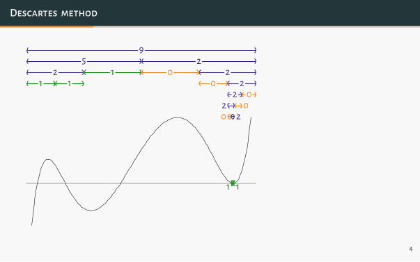
Descartes method
v = 9
9
5 2
5 2
2 1 0 2
2 1 0 2
1 1 0 2
1 1 0 2
2 0
2 0
2 0
2 0
0 2
0 2
1 1
1 1
9
5
2
1 1
1
2
0 2
0 2
2
2
0 2
1 1
0
0
up toO(nτ)
steps
4

Descartes method
v = 9
9
5 2
5 2
2 1 0 2
2 1 0 2
1 1 0 2
1 1 0 2
2 0
2 0
2 0
2 0
0 2
0 2
1 1
1 1
9
5
2
1 1
1
2
0 2
0 2
2
2
0 2
1 1
0
0
up toO(nτ)
steps
4

Descartes method
v = 9
9
5 2
5 2
2 1 0 2
2 1 0 2
1 1 0 2
1 1 0 2
2 0
2 0
2 0
2 0
0 2
0 2
1 1
1 1
9
5
2
1 1
1
2
0 2
0 2
2
2
0 2
1 1
0
0
up toO(nτ)
steps
4

Descartes method
v = 9
9
5 2
5 2
2 1 0 2
2 1 0 2
1 1 0 2
1 1 0 2
2 0
2 0
2 0
2 0
0 2
0 2
1 1
1 1
9
5
2
1 1
1
2
0 2
0 2
2
2
0 2
1 1
0
0
up toO(nτ)
steps
4

Descartes method
v = 9
9
5 2
5 2
2 1 0 2
2 1 0 2
1 1 0 2
1 1 0 2
2 0
2 0
2 0
2 0
0 2
0 2
1 1
1 1
9
5
2
1 1
1
2
0 2
0 2
2
2
0 2
1 1
0
0
up toO(nτ)
steps
4

Descartes method
v = 9
9
5 2
5 2
2 1 0 2
2 1 0 2
1 1 0 2
1 1 0 2
2 0
2 0
2 0
2 0
0 2
0 2
1 1
1 1
9
5
2
1 1
1
2
0 2
0 2
2
2
0 2
1 1
0
0
up toO(nτ)
steps
4

Descartes method
v = 9
9
5 2
5 2
2 1 0 2
2 1 0 2
1 1 0 2
1 1 0 2
2 0
2 0
2 0
2 0
0 2
0 2
1 1
1 1
9
5
2
1 1
1
2
0 2
0 2
2
2
0 2
1 1
0
0
up toO(nτ)
steps
4

Descartes method
v = 9
9
5 2
5 2
2 1 0 2
2 1 0 2
1 1 0 2
1 1 0 2
2 0
2 0
2 0
2 0
0 2
0 2
1 1
1 1
9
5
2
1 1
1
2
0 2
0 2
2
2
0 2
1 1
0
0
up toO(nτ)
steps
4
Descartes method
v = 9
9
5 2
5 2
2 1 0 2
2 1 0 2
1 1 0 2
1 1 0 2
2 0
2 0
2 0
2 0
0 2
0 2
1 1
1 1
9
5
2
1 1
1
2
0 2
0 2
2
2
0 2
1 1
0
0
up toO(nτ)
steps
4

Descartes method
v = 9
9
5 2
5 2
2 1 0 2
2 1 0 2
1 1 0 2
1 1 0 2
2 0
2 0
2 0
2 0
0 2
0 2
1 1
1 1
9
5
2
1 1
1
2
0 2
0 2
2
2
0 2
1 1
0
0
up toO(nτ)
steps
4

Descartes method
v = 9
9
5 2
5 2
2 1 0 2
2 1 0 2
1 1 0 2
1 1 0 2
2 0
2 0
2 0
2 0
0 2
0 2
1 1
1 1
9
5
2
1 1
1
2
0 2
0 2
2
2
0 2
1 1
0
0
up toO(nτ)
steps
4

Complexity (“benchmark problem”)
isolate all roots of an integer polynomial of degree n and coefficient bitsize τ
# roots / tree width: ≤ n min. root separation: ≥ 2−O(nτ)
subdivision rule and subdivision precision overall bitmodel of computation tree size demand complexity
bisection, exact over Z / Q O(nτ) O(n2τ) O(n4τ2)1
bisection, approximate O(nτ) O(nτ) O(n3τ2)
Newton, exact over Z / Q O(n) O(n2τ)∗ O(n3τ)
Newton, approximate O(n) O(nτ)† O(n3 + n2τ)
∗amortized over entire tree: O(nτ) †amortized over entire tree: O(n + τ)
5

Complexity (“benchmark problem”)
isolate all roots of an integer polynomial of degree n and coefficient bitsize τ
# roots / tree width: ≤ n min. root separation: ≥ 2−O(nτ)
subdivision rule and subdivision precision overall bitmodel of computation tree size demand complexity
bisection, exact over Z / Q O(nτ)1 O(n2τ) O(n4τ2)1
bisection, approximate O(nτ) O(nτ) O(n3τ2)
Newton, exact over Z / Q O(n) O(n2τ)∗ O(n3τ)
Newton, approximate O(n) O(nτ)† O(n3 + n2τ)
∗amortized over entire tree: O(nτ) †amortized over entire tree: O(n + τ)
1[Eigenwillig, Sharma, Yap: ISSAC 2006] [Collins: JSC 2016]
5

… of Real Polynomials …
Deficiencies and remedies

Beyond the RealRAM-model
P(x) = 2πx2 − (π + 4√
2)x + 2√
2 = (πx− 2√
2)(2x− 1) ∈ R[x]≈ 6.2831853072x2 − 8.7984469031x + 2.8284271247
12
2√
2π
1
v =?2
? ?
P( 12 ) = 0?
problems with arbitrarily approximable (“bitstream”) coefficients
• no termination on subdivision on an exact root
• precision demand for processing I = (a, b) depends on |P(a)| and |P(b)|
6

Beyond the RealRAM-model
P(x) = 2πx2 − (π + 4√
2)x + 2√
2 = (πx− 2√
2)(2x− 1) ∈ R[x]≈ 6.…x2 − 9.…x + 3.…
12
2√
2π
1
v =?2
? ?
P( 12 ) = 0?
problems with arbitrarily approximable (“bitstream”) coefficients
• no termination on subdivision on an exact root
• precision demand for processing I = (a, b) depends on |P(a)| and |P(b)|
6

Beyond the RealRAM-model
P(x) = 2πx2 − (π + 4√
2)x + 2√
2 = (πx− 2√
2)(2x− 1) ∈ R[x]≈ 6.3…x2 − 8.8…x + 2.8…
12
2√
2π
1
v =?2
? ?
P( 12 ) = 0?
problems with arbitrarily approximable (“bitstream”) coefficients
• no termination on subdivision on an exact root
• precision demand for processing I = (a, b) depends on |P(a)| and |P(b)|
6

Beyond the RealRAM-model
P(x) = 2πx2 − (π + 4√
2)x + 2√
2 = (πx− 2√
2)(2x− 1) ∈ R[x]≈ 6.28…x2 − 8.79…x + 2.83…
12
2√
2π
1
v =?2
? ?
P( 12 ) = 0?
problems with arbitrarily approximable (“bitstream”) coefficients
• no termination on subdivision on an exact root
• precision demand for processing I = (a, b) depends on |P(a)| and |P(b)|
6

Beyond the RealRAM-model
P(x) = 2πx2 − (π + 4√
2)x + 2√
2 = (πx− 2√
2)(2x− 1) ∈ R[x]≈ 6.283…x2 − 8.7984…x + 2.828…
12
2√
2π
1
v =?2
? ?
P( 12 ) = 0?
problems with arbitrarily approximable (“bitstream”) coefficients
• no termination on subdivision on an exact root
• precision demand for processing I = (a, b) depends on |P(a)| and |P(b)|
6

Beyond the RealRAM-model
P(x) = 2πx2 − (π + 4√
2)x + 2√
2 = (πx− 2√
2)(2x− 1) ∈ R[x]≈ 6.2832…x2 − 8.79845…x + 2.8284…
12
2√
2π
1
v =?2
? ?
P( 12 ) = 0?
problems with arbitrarily approximable (“bitstream”) coefficients
• no termination on subdivision on an exact root
• precision demand for processing I = (a, b) depends on |P(a)| and |P(b)|
6
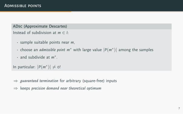
Admissible points
ADsc (Approximate Descartes)Instead of subdivision at m ∈ I:
• sample suitable points near m,
• choose an admissible point m∗ with large value |P(m∗)| among the samples
• and subdivide at m∗.
In particular: |P(m∗)| 6= 0!
⇒ guaranteed termination for arbitrary (square-free) inputs
⇒ keeps precision demand near theoretical optimum
7

Complexity (“benchmark problem”)
isolate all roots of an integer polynomial of degree n and coefficient bitsize τ
# roots / tree width: ≤ n min. root separation: ≥ 2−O(nτ)
subdivision rule and subdivision precision overall bitmodel of computation tree size demand complexity
bisection, exact over Z / Q O(nτ) O(n2τ) O(n4τ2)
bisection, approximate O(nτ) O(nτ)1 O(n3τ2)1
Newton, exact over Z / Q O(n) O(n2τ)∗ O(n3τ)
Newton, approximate O(n) O(nτ)† O(n3 + n2τ)
∗amortized over entire tree: O(nτ) †amortized over entire tree: O(n + τ)
1[Sagraloff: JSC 2014]
8

Clustered roots
v = 9
9
5 2
5 2
2 1 0 2
2 1 0 2
1 1 0 2
1 1 0 2
2 0
2 0
2 0
2 0
0 2
0 2
1 1
1 1
9
5
2
1 1
1
2
0 2
0 2
2
2
0 2
1 1
0
0
up toO(nτ)
steps
9

Clustered roots
v = 9
9
5 2
5 2
2 1 0 2
2 1 0 2
1 1 0 2
1 1 0 2
2 0
2 0
2 0
2 0
0 2
0 2
1 1
1 1
9
5
2
1 1
1
2
0 2
0 2
2
2
0 2
1 1
0
0
up toO(nτ)
steps
9

Clustered roots
v = 9
9
5 2
5 2
2 1 0 2
2 1 0 2
1 1 0 2
1 1 0 2
2 0
2 0
2 0
2 0
0 2
0 2
1 1
1 1
9
5
2
1 1
1
2
0 2
0 2
2
2
0 2
1 1
0
0
up toO(nτ)
steps
9

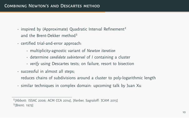
Combining Newton’s and Descartes method
• inspired by (Approximate) Quadratic Interval Refinement2
and the Brent-Dekker method3
• certified trial-and-error approach:
• multiplicity-agnostic variant of Newton iteration• determine candidate subinterval of I containing a cluster• verify using Descartes tests; on failure, resort to bisection
• successful in almost all steps;reduces chains of subdivisions around a cluster to poly-logarithmic length
• similar techniques in complex domain: upcoming talk by Juan Xu
2[Abbott: ISSAC 2006; ACM CCA 2014], [Kerber, Sagraloff: JCAM 2015]3[Brent: 1973]
10

Complexity (“benchmark problem”)
isolate all roots of an integer polynomial of degree n and coefficient bitsize τ
# roots / tree width: ≤ n min. root separation: ≥ 2−O(nτ)
subdivision rule and subdivision precision overall bitmodel of computation tree size demand complexity
bisection, exact over Z / Q O(nτ) O(n2τ) O(n4τ2)
bisection, approximate O(nτ) O(nτ) O(n3τ2)
Newton, exact over Z / Q O(n)1 O(n2τ)∗ O(n3τ)1
Newton, approximate O(n) O(nτ)† O(n3 + n2τ)
∗amortized over entire tree: O(nτ)
†amortized over entire tree: O(n + τ)
1[Sagraloff: ISSAC 2012]
11

Complexity (“benchmark problem”)
isolate all roots of an integer polynomial of degree n and coefficient bitsize τ
# roots / tree width: ≤ n min. root separation: ≥ 2−O(nτ)
subdivision rule and subdivision precision overall bitmodel of computation tree size demand complexity
bisection, exact over Z / Q O(nτ) O(n2τ) O(n4τ2)
bisection, approximate O(nτ) O(nτ) O(n3τ2)
Newton, exact over Z / Q O(n) O(n2τ)∗ O(n3τ)
Newton, approximate O(n) O(nτ)† O(n3 + n2τ)1
∗amortized over entire tree: O(nτ) †amortized over entire tree: O(n + τ)
1[Sagraloff, Mehlhorn: JSC 2016]best known: O(n2τ) [Pan: JSC 2002] [Mehlhorn, Sagraloff, Wang: JSC 2015]
11

… and now For Real!
Implementation results

Implementation
RS
• C library for real root solving, refinement & more
• sophisticated implementation of classical Descartes
• tailored for approximate arithmetic
• high-performance general purpose solver
• default real root solver in Maple since version 11
[Rouillier, Zimmermann: JCAM 2003]
12

Implementation
ANewDsc (Approximate Arithmetic Newton-Descartes)
• implemented on top of RS
• merged admissible point selection & Newton-Descartes
• heuristics to reduce / eliminate overhead on “easy” instances
• additional optimizations
• certified output (based on interval arithmetic using MPFI)
• matches theoretical worst-case bit complexity (Las Vegas)(assuming asymptotically fast polynomial arithmetic)
• to be integrated in Maple 201x?
[Sagraloff, Mehlhorn: JSC 2016]
12

Benchmark excerpt: tame (well-separated) instances
instance degree bitsizeRS ANewDsc
speeduptime [s] nodes time [s] nodes
random 16384 1024 275.1 46 279.0 40 0.99Hermite 1024 9875 88.3 2237 79.6 1396 1.11Legendre 1024 4640 118.2 2272 117.2 1325 1.01Wilkinson 1024 8777 219.1 2064 398.8 1565 0.73
13

Benchmark excerpt: hard (clustered) instances
instance degree bitsizeRS ANewDsc
speeduptime [s] nodes time [s] nodes
monic random 4096 1024 713.1 3212 14.6 37 48.84random2 − 1 1024 1029 288.5 6648 5.2 419 55.48
14

Benchmark excerpt: hard (clustered) instances
instance degree bitsizeRS ANewDsc
speeduptime [s] nodes time [s] nodes
Mignotte polynomials: xn − (ax− 1)2
a = 231 1025 63 3.6 66 1.4 27 2.57a = 5 1025 5 402.6 2384 0.7 43 575.14a = 231 + 1 1025 63 13338.4 31810 1.2 53 11115.3
two clustered roots near 1/awith separation of appx. an/2
14

Comparison to other solvers
instance n τ MPSolve CF Sage RS ANewDsc
random 16384 1024 578.9 376.6 3825.1 275.1 279.0Hermite 1024 9875 2169.9 140.5 11.9 88.3 79.6Legendre 1024 4640 5061.3 79.0 9.7 118.2 117.2Wilkinson 1024 8777 5308.1 13.7 14.1 219.1 398.8
random2 − 1 512 1029 33.5 339.2 3.1 71.5 1.31024 1029 141.8 > 7200 8.2 288.5 5.2
random monic 1024 1024 2.6 0.7 4115.0 38.8 1.216384 1024 579.3 279.2 > 7200 > 7200 143.1
xn − (2ax− 1)2 2047 5 87.2 1.2 21.1 1.0 1.2xn − (ax− 1)2 2047 5 131.5 1.5 21.7 1.6 1.6xn − (ax2 − 1)2 2047 5 99.1 > 7200 26.5 3472.0 8.3nested 4-fold 260 2560 69.6 348.8 5.6 636.7 2.1
1028 260 186.2 3993.7 20.9 430.4 7.4
15

Bit complexity estimation: tame instances
16K 32K 48K
2k
4k
6k
n
time [s]
estimated exponent for degree: 1.97
16K 32K 48K 64K
10
20
τ
time [s]
estimated exponent for bitsize: −0.03
theoretical vs. estimated bit complexity:O(n3 + n2τ) vs. O(n1.97τ−0.03)
degree n, integer coefficients in range (−2τ, 2τ) chosen uniformly at randomleft: τ = 1024; right: n = 1024
16

Bit complexity estimation: hard instances
1K 2K 3K
500
1k
n
time [s]
estimated exponent for degree: 2.37
1.5K 3K 4.5K
100
200
300
τ
time [s]
estimated exponent for bitsize: 1.45
theoretical vs. estimated bit complexity:O(n3 + n2τ) vs. O(n2.37τ1.45)
Mignotte-like: xn − (ax2 − 1)3 (cluster of multiplicity 3 around irrational center)left: a = 2256 − 1; right: n = 1024
17
ANewDsc: Approximate Arithmetic Newton-Descartes
• highly efficient general-purpose solver
• tremendous speedups in degenerate situationswithout tailored tweaks (e.g., does not (yet) exploit sparsity)
no
• easily solves previously infeasible instances
• first available solver with
• expected performance near theoretical optimum• native support for inputs with arbitrary real coefficients
• implementation & benchmarks available at ANewDsc.mpi-inf.mpg.de
Thank you for your attention!
18


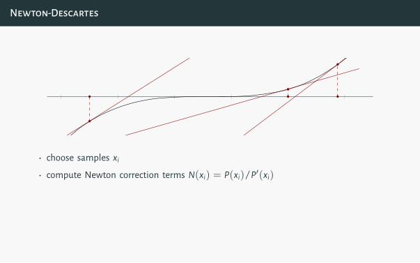
Newton-Descartes
0 0
• choose samples xi
• compute Newton correction terms N(xi) = P(xi)/P′(xi)
• guess multiplicity k s.t. xi − k · N(xi) is approximately the same
• verify that no roots are lost; otherwise, resort to bisection
Newton-Descartes
0 0
• choose samples xi
• compute Newton correction terms N(xi) = P(xi)/P′(xi)
• guess multiplicity k s.t. xi − k · N(xi) is approximately the same
• verify that no roots are lost; otherwise, resort to bisection

Newton-Descartes
0 0
• choose samples xi
• compute Newton correction terms N(xi) = P(xi)/P′(xi)
• guess multiplicity k s.t. xi − k · N(xi) is approximately the same
• verify that no roots are lost; otherwise, resort to bisection

Newton-Descartes
0 0
• choose samples xi
• compute Newton correction terms N(xi) = P(xi)/P′(xi)
• guess multiplicity k s.t. xi − k · N(xi) is approximately the same
• verify that no roots are lost; otherwise, resort to bisection


Comparison to other solvers
instance n τ MPSolve CF Sage SLV RS ANewDsc
random 16384 1024 578.9 376.6 3825.1 5138.1 275.1 279.0Hermite 1024 9875 2169.9 140.5 11.9 176.3 88.3 79.6Legendre 1024 4640 5061.3 79.0 9.7 215.2 118.2 117.2Wilkinson 1024 8777 5308.1 13.7 14.1 (80.9) 219.1 398.8
random2 − 1 512 1029 33.5 339.2 3.1 3270.5 71.5 1.31024 1029 141.8 > 7200 8.2 > 7200 288.5 5.2
random monic 1024 1024 2.6 0.7 4115.0 > 7200 38.8 1.216384 1024 579.3 279.2 > 7200 > 7200 > 7200 143.1
xn − (2ax− 1)2 2047 5 87.2 1.2 21.1 1.1 1.0 1.2xn − (ax− 1)2 2047 5 131.5 1.5 21.7 0.7 1.6 1.6xn − (ax2 − 1)2 2047 5 99.1 > 7200 26.5 > 7200 3472.0 8.3nested 4-fold 260 2560 69.6 348.8 5.6 1193.9 636.7 2.1
1028 260 186.2 3993.7 20.9 6983.4 430.4 7.4