Computing Query Probability with Incidence Algebras

Nilesh DalviYahoo Research

Santa Clara, CA, USAndalvi@yahoo-inc.com

Karl SchnaitterUC Santa Cruz

Santa Cruz, CA, USAkarlsch@soe.ucsc.edu

Dan SuciuUniversity of Washington

Seattle, WA, USAsuciu@cs.washington.edu

ABSTRACTWe describe an algorithm that evaluates queries over probabilisticdatabases using Mobius’ inversion formula in incidence algebras.The queries we consider are unions of conjunctive queries (equiv-alently: existential, positive First Order sentences), and the proba-bilistic databases are tuple-independent structures. Our algorithmruns in PTIME on a subset of queries called "safe" queries, and iscomplete, in the sense that every unsafe query is hard for the classFP#P . The algorithm is very simple and easy to implement inpractice, yet it is non-obvious. Mobius’ inversion formula, whichis in essence inclusion-exclusion, plays a key role for completeness,by allowing the algorithm to compute the probability of some safequeries even when they have some subqueries that are unsafe. Wealso apply the same lattice-theoretic techniques to analyze an algo-rithm based on lifted conditioning, and prove that it is incomplete.

Categories and Subject DescriptorsH.2.4 [Database Management]: Systems—Query Processing; F.4.1[Mathematical Logic and Formal Languages]: Mathematical Logic

General TermsAlgorithms, Theory

KeywordsMobius inversion, incidence algebra, probabilistic database

1. INTRODUCTIONIn this paper we show how to use incidence algebras to evaluate

unions of conjunctive queries over probabilistic databases. Thesequeries correspond to the select-project-join-union fragment of therelational algebra, and they also correspond to existential positiveformulas of First Order Logic. A probabilistic database, also re-ferred to as a probabilistic structure, is a pair (A, P ) where A =(A,RA1 , . . .,RAk ) is first order structure over vocabularyR1, . . . , Rk,and P is a function that associates to each tuple t in A a numberP (t) ∈ [0, 1]. A probabilistic structure defines a probability distri-bution on the set of substructures B of A by:

Permission to make digital or hard copies of all or part of this work forpersonal or classroom use is granted without fee provided that copies arenot made or distributed for profit or commercial advantage and that copiesbear this notice and the full citation on the first page. To copy otherwise, torepublish, to post on servers or to redistribute to lists, requires prior specificpermission and/or a fee.PODS’10, June 6–11, 2010, Indianapolis, Indiana, USA.Copyright 2010 ACM 978-1-4503-0033-9/10/06 ...$10.00.

PA(B) =

k∏i=1

(∏t∈RB

i

P (t)×∏

t∈RAi −R

Bi

(1− P (t))) (1)

We describe a simple, yet quite non-obvious algorithm for com-puting the probability of an existential, positive FO sentence Φ,PA(Φ)1, based on Mobius’ inversion formula in incidence alge-bras. The algorithm runs in polynomial time in the size of A. Thealgorithm only applies to certain sentences, called safe sentences,and is sound and complete in the following way. It is sound, inthat it computes correctly the probability for each safe sentence,and it is complete in that, for every fixed unsafe sentence Φ, thedata complexity of computing Φ is FP#P -hard. This establishesa dichotomy for the complexity of unions of conjunctive queriesover probabilistic structures. The algorithm is more general than,and significantly simpler than a previous algorithm for conjunctivesentences [5].

The existence of FP#P -hard queries on probabilistic structureswas observed by Grädel et al. [8] in the context of query reliabil-ity. In the following years, several studies [4, 6, 11, 10], sought toidentify classes of tractable queries. These works provided condi-tions for tractability only for conjunctive queries without self-joins.The only exception is [5], which considers conjunctive queries withself-joins. We extend those results to a larger class of queries, andat the same time provide a very simple algorithm. Some other priorwork is complimentary to ours, e.g., the results that consider theeffects of functional dependencies [11].

Our results have applications to probabilistic inference on pos-itive Boolean expressions [7]. For every tuple t in a structure A,let Xt be a distinct Boolean variable. Every existential positiveFO sentence Φ defines a positive DNF Boolean expression over thevariables Xt, sometimes called lineage expression, whose proba-bility is the same as PA(Φ). Our result can be used to classify thecomplexity of computing the probability of Positive DNF formulasdefined by a fixed sentence Φ. For example, the two sentences2

Φ1 = R(x), S(x, y) ∨ S(x, y), T (y) ∨R(x), T (y)

Φ2 = R(x), S(x, y) ∨ S(x, y), T (y)

define two classes of positive Boolean DNF expressions (lineages):

F1 =∨

a∈R,(a,b)∈SXaYa,b ∨

∨(a,b)∈S,b∈T

Ya,b, Zb ∨∨

a∈R,b∈SXaYb

F2 =∨

a∈R,(a,b)∈SXaYa,b ∨

∨(a,b)∈S,b∈T

Ya,b, Zb

1This is the marginal probability PA(Φ) =∑

B:B|=Φ PA(B).2We omit quantifiers and drop the conjunct they are clear from thecontext, e.g. Φ2 = ∃x∃y(R(x) ∧ S(x, y) ∨ S(x, y) ∧ T (y)).

Our result implies that, for each such class of Boolean formulas, ei-ther all formulas in that class can be evaluated in PTIME in the sizeof the formula, or the complexity for that class is hard for FP#P ;e.g. F1 can be evaluated in PTIME using our algorithm, while F2

is hard.The PTIME algorithm we present here relies in a critical way

on an interesting connection between existential positive FO sen-tences and incidence algebras [16]. By using the Mobius inversionformula in incidence algebras we resolve a major difficulty of theevaluation problem: a sentence that is in PTIME may have a subex-pression that is hard. This is illustrated by Φ1 above, which is inPTIME, but has Φ2 as a subexpression, which is hard; to evaluateΦ1 one must avoid trying to evaluate Φ2. Our solution is to ex-press P (Φ) using Mobius’ inversion formula: subexpressions ofΦ that have a Mobius value of zero do not contribute to P (Φ),and this allows us to compute P (Φ) without computing its hardsubexpressions. The Mobius inversion formula corresponds to theinclusion/exclusion principle, which is ubiquitous in probabilisticinference: the connection between the two in the context of prob-abilistic inference has already been recognized in [9]. However, tothe best of our knowledge, ours is the first application that exploitsthe full power of Mobius inversion to remove hard subexpressionsfrom a computation of probability.

Another distinguishing, and quite non-obvious aspect of our ap-proach is that we apply our algorithm on the CNF, rather than themore commonly used DNF representation of existential, positiveFO sentences. This departure from the common representation ofexistential, positive FO is necessary in order to handle correctlyexistential quantifiers.

We call sentences on which our algorithm works safe; those onwhich the algorithm fails we call unsafe. We prove a theorem stat-ing that the evaluation problem of a safe query is in PTIME, andof an unsafe query is hard for FP#P : this establishes both thecompleteness of our algorithm and a dichotomy of all existential,positive FO sentences. The proof of the theorem is in two steps.First, we define a simple class of sentences called forbidden sen-tences, where each atom has at most two variables, and a set ofsimple rewrite rules on existential, positive FO sentences; we provethat the safe sentences can be characterized as those that cannot berewritten into a forbidden sentence. Second, we prove that everyforbidden sentence is hard for FP#P , using a direct, and ratherdifficult proof which we include in [3]. Together, these two resultsprove that every unsafe sentence is hard for FP#P , establishingthe dichotomy. Notice that our characterization of safe queries isreminiscent of minors in graph theory. There, a graph H is calleda minor of a graph G if H can be obtained from G through a se-quence of edge contractions. “Being a minor of” defines a partialorder on graphs: Robertson and Seymour’s celebrated result statesthat any minor-closed family is characterized by a finite set of for-bidden minors. Our characterization of safe queries is also donein terms of forbidden minors, however the order relation is morecomplex and the set of forbidden minors is infinite.

In the last part of the paper, we make a strong claim: that us-ing Mobius’ inversion formula is a necessary technique for com-pleteness. Today’s approaches to general probabilistic inferencefor Boolean expressions rely on combining (using some advancedheuristics) a few basic techniques: independence, disjointness, andconditioning. In conditioning, one chooses a Boolean variable X ,then computes P (F ) = P (F | X)P (X) + P (F | ¬X)(1 −P (X)). We extended these techniques to unions of conjunctivequeries, an approach that is generally known as lifted inference [12,15, 14] and given a PTIME algorithm based on these three tech-niques. The algorithm performs conditioning on subformulas of

Φ instead of Boolean variables. We prove that this algorithm isnot complete, by showing a formula Φ (Fig. 2) that is computablein PTIME, but for which it is not possible to compute using liftedinference that combines conditioning, independence, and disjoint-ness on subformulas. On the other hand, we note that condition-ing has certain practical advantages that are lost by Mobius’ inver-sion formula: by repeated conditioning on Boolean variables, onecan construct a Free Binary Decision Diagram [17], which has fur-ther applications beyond probabilistic inference. There seems to beno procedure to convert Mobius’ inversion formula into FBDDs;in fact, we conjecture that the formula in Fig. 2 does not have anFBDD whose size is polynomial in that of the input structure.

Finally, we mention that a different way to define classes ofBoolean formulas has been studied in the context of the constraintsatisfaction problem (CSP). Creignou et al. [2, 1] showed that thecounting version of the CSP problem has a dichotomy into PTIMEand FP#P -hard. These results are orthogonal to ours: they de-fine the class of formulas by specifying the set of Boolean opera-tors, such as and/or/not/majority/parity etc, and do not restrict theshape of the Boolean formula otherwise. As a consequence, theonly class where counting is in PTIME is defined by affine opera-tors: all classes of monotone formulas are hard. In contrast, in ourclassification there exist classes of formulas that are in PTIME, forexample the class defined by Φ1 above.

2. BACKGROUND AND OVERVIEWPrior Results A very simple PTIME algorithm for conjunctive

queries without self-joins is discussed in [4, 6]. When the conjunc-tive query is connected, the algorithm chooses a variable that occursin all atoms (called a root variable) and projects it out, comput-ing recursively the probabilities of the sub-queries; if no root vari-able exists, then the query is FP#P -hard. When the conjunctivequery is disconnected, then the algorithm computes the probabili-ties of the connected components, then multiples them. Thus, thealgorithm alternates between two steps, called independent projec-tion, and independent join. For example, consider the conjunctivequery3:

ϕ = R(x, y), S(x, z)

The algorithm computes its probability by performing the fol-lowing steps:

P (ϕ) = 1−∏a∈A

(1− P (R(a, y), S(a, z)))

P (R(a, y), S(a, z)) = P (R(a, y)) · P (S(a, z))

P (R(a, y)) = 1−∏b∈A

(1− P (R(a, b)))

P (S(a, z)) = 1−∏c∈A

(1− P (S(a, c)))

The first line projects out the root variable x, where A is theactive domain of the probabilistic structure: it is based on fact that,in ϕ ≡

∨a∈A(R(a, y), S(a, z)), the sub-queries R(a, y), S(a, z)

are independent for distinct values of the constant a. The secondline applies independent join; and the third and fourth lines applyindependent project again.

This simple algorithm, however, cannot be applied to a querywith self-joins because both the projection and the join step are in-correct. For a simple example, considerR(x, y), R(y, z). Here y isa root variable, but the queriesR(x, a), R(a, z) andR(x, b), R(b, z)

3All queries are Boolean and quantifiers are dropped; in completenotation, ϕ is ∃x.∃y.∃z.R(x, y), S(x, z).

are dependent (both depend on R(a, b) and R(b, a)). Hence, it isnot possible to do an independent projection on y. In fact, thisquery is FP#P -hard.

Queries with self-joins were analyzed in [5] based on the no-tion of an inversion. In a restricted form, an inversion consists oftwo atoms, over the same relational symbol, and two positions inthose atoms, such that the first position contains a root variable inthe first atom and a non-root variable in the second atom, and thesecond position contains a non-root / root pair of variables. In ourexample above, the atoms R(x, y) and R(y, z) and the positions 1and 2 form an inversion: position 1 has variables x and y (non-root/ root) and position 2 has variables y and z (root / non-root). Thepaper describes a first PTIME algorithm for queries without inver-sions, by expressing its probability in terms of several sums, eachof which can be reduced to a polynomial size expression. Then,the paper notices that some queries with inversion can also be com-puted in polynomial time, and describes a second PTIME algorithmthat uses one sum (called eraser) to cancel the effect of a another,exponentially sized sum. The algorithm succeeds if it can erase allexponentially sized sums (corresponding to sub-queries with inver-sions).

Our approach The algorithm that we describe in this paper isboth more general (it applies to unions of conjunctive queries), andsignificantly simpler than either of the two algorithms in [5]. Weillustrate it here on a conjunctive query with a self-join (S occurstwice):

ϕ = R(x1), S(x1, y1), S(x2, y2), T (x2)

Our algorithm starts by applying the inclusion-exclusion formula:

P (R(x1), S(x1, y1), S(x2, y2), T (x2)) =

P (R(x1), S(x1, y1)) + P (S(x2, y2), T (y2))

−P (R(x1), S(x1, y1) ∨ S(x2, y2), T (x2))

This is the dual of the more popular inclusion-exclusion formulafor disjunctions; we describe it formally in the framework of inci-dence algebras in Sec. 3. The first two queries are without self-joinsand can be evaluated as before. To evaluate the query on the lastline, we simultaneously project out both variables x1, x2, writingthe query as:

ψ =∨a∈A

(R(a), S(a, y1) ∨ S(a, y2), T (a))

The variables x1, x2 are chosen because they satisfy the follow-ing conditions: they occur in all atoms, and for the atoms with thesame relation name (S in our case) they occur in the same position.We call such a set of variables separator variables (Sec. 4). Asa consequence, sub-queries R(a), S(a, y1) ∨ S(a, y2), T (a) cor-responding to distinct constants a are independent. We use thisindependence, then rewrite the sub-query into CNF and apply theinclusion/exclusion formula again:

P (ψ) = 1−∏a∈A

(1− P (R(a), S(a, y1) ∨ S(a, y2), T (a)))

R(a), S(a, y1) ∨ S(a, y2), T (a) ≡ (R(a) ∨ T (a)) ∧ S(a, y)

P ((R(a) ∨ T (a)) ∧ S(a, y))

= P (R(a) ∨ T (a)) + P (S(a, y))− P (R(a) ∨ T (a) ∨ S(a, y))

= P (R(a)) + P (T (a))− P (R(a)) · P (T (a))

−1 + (1− P (R(a)))(1− P (T (a)))∏b∈A

(1− P (S(a, b)))

In summary, the algorithm alternates between applying the inclu-sion/exclusion formula, and performing a simultaneous projection

on separator variables: when no separator variables exists, then thequery is FP#P -hard. The two steps can be seen as generaliza-tions of the independent join, and the independent projection forconjunctive queries without self-joins.

Ranking Before running the algorithm, a rewriting of the queryis necessary. Consider R(x, y), R(y, x): it has no separator vari-able because neither x nor y occurs in both atoms on the same posi-tion. After a simple rewriting, however, the query can be evaluatedby our algorithm: partition the relation R(x, y) into three sets, ac-cording to x < y, x = y, x > y, call them R<, R=, R>, andrewrite the query as R<(x, y), R>(y, x) ∨ R=(z). Now x, z is aseparator, because the three relational symbols are distinct. We callthis rewriting ranking (Sec. 5). It needs to be done only once, be-fore running the algorithm, since all sub-queries of a ranked queriesare ranked. A similar but more general rewriting called coveragewas introduced in [5]: ranking corresponds to the canonical cover-age.

Incidence Algebras An immediate consequence of using theinclusion-exclusion formula is that sub-queries that happen to can-cel out do not have to be evaluated. This turns out to be a funda-mental property of the algorithm that allows it to be complete since,as we have explained, some queries are in PTIME but may havesub-queries that are hard. This cancellation is described by the Mo-bius inversion formula, which groups equal terms in the inclusion-exclusion expansion under coefficients called the Mobius function.Using this notion, it is easy to state when a query is PTIME: thishappens if and only if all its sub-queries that have a non-zero Mo-bius function are in PTIME. Thus, while the algorithm itself couldbe described without any reference to the Mobius inversion for-mula, by simply using inclusion-exclusion, the Mobius functiongives a key insight into what the algorithm does: it recurses onlyon sub-queries whose Mobius function is non-zero. In fact, weprove the following result (Theorem 6.6): for every finite lattice,there exists a query whose sub-queries generate precisely that lat-tice, such that all sub-queries are in PTIME except that correspond-ing to the bottom of the lattice. Thus, the query is in PTIME iff theMobius function of the lattice bottom is zero. In other words, anyformulation of the algorithm must identify, in some way, the ele-ments with a zero Mobius function in an arbitrary lattice: queriesare as general as any lattice. For that reason we prefer to exposethe Mobius function in the algorithm rather than hide it under theinclusion/exclusion formula.

Lifted Inference At a deeper level, lattices and their associatedMobius function help us understand the limitations of alternativequery evaluation algorithms. In Sec. 7 we study an evaluation al-gorithm based on lifted conditioning and disjointness. We showthat conditioning is equivalent to replacing the lattice of sub-querieswith a certain sub-lattice. By repeated conditioning one it is some-times possible to simplify the lattice sufficiently to remove all hardsub-queries whose Mobius function is zero. However, we given anexample of a lattice with 9 elements (Fig 2) whose bottom elementhas the Mobius function equal to zero, but where no conditioningcan further restrict the lattice. Thus, the algorithm based on liftedconditioning makes no progress on this lattice, and cannot evaluatethe corresponding query. By contrast, our algorithm based on Mo-bius’ inversion formula will easily evaluate the query by skippingthe bottom element (since its Mobius function is zero). Thus, ournew algorithm based on Mobius’ inversion formula is more gen-eral than existing techniques based on lifted inference. Finally, wecomment on the implications for the completeness of the algorithmin [5].

In the rest of the paper we will refer to conjunctive queries andunions of conjunctive queries as conjunctive sentences, and exis-

tential positive FO sentences (or just positive FO sentences) respec-tively.

3. EXISTENTIAL POSITIVE FO AND IN-CIDENCE ALGEBRAS

We describe here the connection between positive FO and inci-dence algebras. We start with basic notations.

3.1 Existential Positive FOFix a vocabulary R̄ = {R1, R2, . . .}. A conjunctive sentence

ϕ is a first-order logical formula obtained from positive relationalatoms using ∧ and ∃:

ϕ = ∃x̄.(r1 ∧ . . . ∧ rk) (2)

We allow the use of constants. V ar(ϕ) = x̄ denotes the set ofvariables in ϕ, and Atoms(ϕ) = {r1, . . . , rk} the set of atoms.Consider the undirected graph where the nodes are Atoms(ϕ) andedges are pairs (ri, rj) s.t. ri, rj have a common variable. A com-ponent of ϕ is a connected component in this graph. Each conjunc-tive sentence ϕ can be written as:

ϕ = γ1 ∧ . . . ∧ γp

where each γi is a component; in particular, γi and γj do not shareany common variables, when i 6= j.

A disjunctive sentence is an expression of the form:

ϕ′ = γ′1 ∨ . . . ∨ γ′qwhere each γ′i is a single component.

An existential, positive sentence Φ is obtained from positive atomsusing ∧, ∃ and ∨; we will refer to it briefly as positive sentence. Wewrite a positive sentence either in DNF or in CNF:

Φ = ϕ1 ∨ . . . ∨ ϕm (3)Φ = ϕ′1 ∧ . . . ∧ ϕ′M (4)

where ϕi are conjunctive sentences in DNF (3), and ϕ′i are disjunc-tive sentences in CNF (4). The DNF can be rewritten into the CNFby:

Φ =∨

i=1,m

∧j=1,pi

γij =∧f

∨i

γif(i)

where f ranges over functions with domain [m] s.t. ∀i ∈ [m],f(i) ∈ [pi]. This rewriting can increase the size of the sentenceexponentially4. Finally, we will often drop ∃ and ∧ when clearfrom the context.

A classic result by Sagiv and Yannakakis [13] gives a necessaryand sufficient condition for a logical implication of positive sen-tences written in DNF: if Φ =

∨i ϕi and Φ′ =

∨j ϕ′j , then:

Φ⇒ Φ′ iff ∀i.∃j.ϕi ⇒ ϕ′j (5)

No analogous property holds for CNF: R(x, a), S(a, z) logicallyimplies R(x, y), S(y, z) (where a is a constant), but R(x, a) 6⇒R(x, y), S(y, z) and S(a, z) 6⇒ R(x, y), S(y, z). We show inSec. 5 a rewriting technique that enforces such a property.

3.2 Incidence AlgebrasNext, we review the basic notions in incidence algebras follow-

ing Stanley [16]. A finite lattice is a finite ordered set (L̂,≤)

where every two elements u, v ∈ L̂ have a least upper bound4Our algorithm runs in PTIME data complexity; we do not addressthe expression complexity in this paper.

u ∨ v and a greatest lower bound u ∧ v, usually called join andmeet. Since it is finite, it has a minimum and a maximum ele-ment, denoted 0̂, 1̂. We denote L = L̂− {1̂} (departing from [16],where L denotes L̂ − {0̂, 1̂}). L is a meet-semi-lattice. The in-cidence algebra I(L̂) is the algebra5 of real (or complex) matri-ces t of dimension |L̂| × |L̂|, where the only non-zero elementstuv (denoted t(u, v)) are for u ≤ v; alternatively, a matrix canbe seen as a linear function t : RL̂ → RL̂. Two matrices areof key importance in incidence algebras: ζL̂ ∈ I(L̂), defined asζL̂(u, v) = 1 forall u ≤ v; and its inverse, the Mobius functionµL̂ : {(u, v) | u, v ∈ L̂, u ≤ v} → Z, defined by:

µL̂(u, u) = 1

µL̂(u, v) = −∑

w:u<w≤v

µL̂(w, v)

We drop the subscript and write µwhen L̂ is clear from the context.The fact that µ is the inverse of ζ means the following thing.

Let f : L̂ → R be a real function defined on the lattice. De-fine a new function g as g(v) =

∑u≤v f(u). Then f(v) =∑

u≤v µ(u, v)g(u). This is called Mobius’ inversion formula, andis a key piece of our algorithm. Note that it simply expresses thefact that g = ζ(f) implies f = µ(g).

3.3 Their ConnectionA labeled lattice is a triple L̂ = (L̂,≤, λ) where (L̂,≤) is a lat-

tice and λ assigns to each element in u ∈ L̂ a positive FO sentenceλ(u) s.t. λ(u) ≡ λ(v) iff u = v.

DEFINITION 3.1. A D-lattice is a labeled lattice L̂ where, forallu 6= 1̂, λ(u) is conjunctive, forall u, v, λ(u∧ v) is logically equiv-alent to λ(u) ∧ λ(v), and λ(1̂) ≡

∨u<1̂ λ(u).

A C-lattice is a labeled lattice L̂ where, forall u 6= 1̂, λ(u) isdisjunctive, forall u, v, λ(u ∧ v) is logically equivalent to λ(u) ∨λ(v), and λ(1̂) =

∧u<1̂ λ(u).

In a D-lattice, u ≤ v iff λ(u) ⇒ λ(v). This is because λ(u) =λ(u ∧ v) is logically equivalent to λ(u) ∧ λ(v). Similarly, in aC-lattice, u ≤ v iff λ(v)⇒ λ(u). If L̂ is a D- or C-lattice, we sayL̂ represents Φ = λ(1̂).

PROPOSITION 3.2 (INVERSION FORMULA FOR POSITIVE FO).Fix a probabilistic structure (A, P ) and a positive sentence Φ; de-note PA as P . Let L̂ be either a D-lattice or a C-lattice represent-ing Φ. Then:

P (Φ) = P (λ(1̂)) = −∑v<1̂

µL(v, 1̂)P (λ(v)) (6)

PROOF. The proof for the D-lattice is from [16]. Denote f(u) =P (λ(u) ∧ ¬(

∨v<u λ(v))). Then:

P (λ(u)) =∑v≤u

f(v) ⇒ f(u) =∑v≤u

µ(v, u)P (λ(v))

The claim follows by setting u = 1̂ and noting f(1̂) = 0. For aC-lattice, write λ′(u) = ¬λ(u). Then P (λ(1̂)) = 1−P (λ′(1̂)) =1+

∑v<1̂ µ(v, 1̂)P (λ′(v)) and the claim follows from the fact that∑

v∈L̂ µ(v, 1̂) = 0.

5An algebra is a vector space plus a multiplication operation [16].

1̂

ϕ1 ϕ3 ϕ2

ϕ1,ϕ3 ϕ2,ϕ3

0̂ = ϕ1,ϕ2,ϕ3

1̂

ϕ4 ϕ5

0̂ = ϕ4 ∨ ϕ5

(a) (b)

1̂

ϕ1 ϕ2 ϕ3

ϕ1,ϕ2 ϕ1,ϕ3 ϕ2,ϕ3

ϕ4

0̂ = ϕ1,ϕ2,ϕ3,ϕ4

1

1̂

ϕ1 ϕ3 ϕ2

ϕ1,ϕ3 ϕ2,ϕ3

0̂ = ϕ1,ϕ2,ϕ3

1̂

ϕ4 ϕ5

0̂ = ϕ4 ∨ ϕ5

(a) (b)

1̂

ϕ1 ϕ2 ϕ3

ϕ1,ϕ2 ϕ1,ϕ3 ϕ2,ϕ3

ϕ4

0̂ = ϕ1,ϕ2,ϕ3,ϕ4

1

(a) (b)

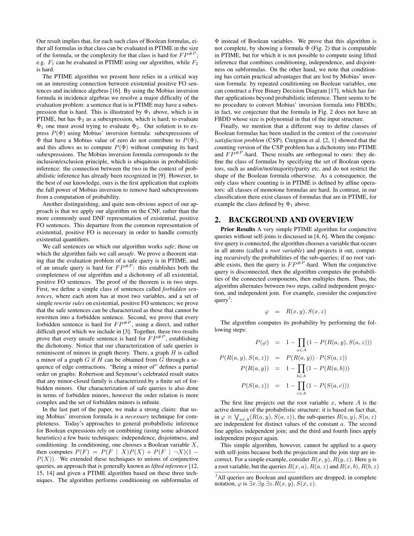
Figure 1: The D-lattice (a) and the C-lattice (b) for Φ (Ex. 3.3).

The proposition generalizes the well known inclusion/exclusionformula (for D-lattices), and its less well known dual (for C-lattices):

P (a ∨ b ∨ c) = P (a) + P (b) + P (c)

−P (a ∧ b)− P (a ∧ c)− P (b ∧ c) + P (a ∧ b ∧ c)P (a ∧ b ∧ c) = P (a) + P (b) + P (c)

−P (a ∨ b)− P (a ∨ c)− P (b ∨ c) + P (a ∨ b ∨ c)

We show how to construct a canonical D-lattice, L̂D(Φ) thatrepresents a positive sentence Φ. Start from the DNF in Eq.(3), andfor each subset s ⊆ [m] denote ϕs =

∧i∈s ϕi. Let L̂ be the set of

these conjunctive sentences, up to logical equivalence, and orderedby logical implication (hence, |L| ≤ 2m). Label each elementu ∈ L̂, u 6= 1̂, with its corresponding ϕs (choose any, if thereare multiple equivalent ones), and label 1̂ with

∨s 6=∅ ϕs (≡ Φ).

We denote the resulting D-lattice L̂D(Φ). Similarly, L̂C(Φ) is theC-lattice that represents Φ, obtained from the CNF of Φ in Eq.(4),setting ϕ′s =

∨i∈s ϕ

′i.

The first main technique of our algorithm is this. Given Φ, com-pute its C-lattice, then use Eq.(6) to compute P (Φ); we explainlater why we use the C-lattice instead of the D-lattice. It remainsto compute the probability of disjunctive sentences P (λ(u)): weshow this in the next section. The power of this technique comesfrom the fact that, whenever µ(u, 1̂) = 0, then we do not needto compute the corresponding P (λ(u)). As we explain in Sec. 7this is strictly more powerful than the current techniques used inprobabilistic inference, such as lifted conditioning.

Example 3.3 Consider the following positive sentence:

Φ = R(x1), S(x1, y1) ∨ S(x2, y2), T (y2) ∨R(x3), T (y3)

= ϕ1 ∨ ϕ2 ∨ ϕ3

The Hasse diagram of the D-lattice LD(Φ) is shown in Fig. 1 (a).There are eight subsets s ⊆ [3], but only seven up to logical equiv-alence, because6 ϕ1, ϕ2 ≡ ϕ1, ϕ2, ϕ3. The values of the Mobiusfunction are, from top to bottom: 1,−1,−1,−1, 1, 1, 0, hence theinversion formula is7:

P (Φ) = P (ϕ1) + P (ϕ2) + P (ϕ3)− P (ϕ1ϕ3)− P (ϕ2ϕ3)

The Hasse diagram of the C-lattice LC(Φ) is shown in Fig. 1

6There exists a homomorphism ϕ1, ϕ2, ϕ3 → ϕ1, ϕ2 that mapsR(x3) to R(x1) and T (y3) to T (y2).7One can arrive at the same expression by using inclusion-exclusion instead of Mobius’ inversion formula, and noting thatϕ1, ϕ2 ≡ ϕ1, ϕ2ϕ3, hence these two terms cancel out in theinclusion-exclusion expression.

(b). To see this, first express Φ in CNF:

Φ = (R(x1), S(x1, y1) ∨ S(x2, y2), T (y2) ∨R(x3)) ∧(R(x4), S(x4, y4) ∨ S(x5, y5), T (y5) ∨ T (y6))

= (R(x3) ∨ S(x2, y2), T (y2)) ∧ (R(x4), S(x4, y4) ∨ T (y6))

= ϕ4 ∧ ϕ5

Note that 0̂ is labeled withϕ4∨ϕ5 ≡ R(x3)∨T (y6). The inversionformula here is:

P (Φ) = P (ϕ4) + P (ϕ5)− P (ϕ4 ∨ ϕ5)

where ϕ4 ∨ ϕ5 ≡ R(x3) ∨ T (y6).

3.4 MinimizationBy minimizing a conjunctive sentence ϕ we mean replacing it

with an equivalent sentence ϕ0 that has the smallest number ofatoms. A disjunctive sentence Φ =

∨γi is minimized if every

conjunctive sentence is minimized and there is no homomorphismϕi ⇒ ϕj for i 6= j. If such a homomorphism exists, then wecall ϕj redundant: clearly we can remove it from the expression Φwithout affecting its semantics.

For the purpose of D-lattices, it doesn’t matter if we minimize thesentence or not: if the sentence is not minimized, then one can showthat all lattice elements corresponding to redundant terms have theMobius function equal to zero. More precisely, any two D-latticesthat represent the same sentence have the same set of elements witha non-zero Mobius function: we state this fact precisely in the re-mainder of this section. A similar fact does not hold in general forC-lattices, but it holds over ranked structures (Sec. 5.2).

An element u in a lattice covers v if u > v and there is no w s.t.u > w > v. An atom8 is an element that covers 0̂; a co-atom is anelement covered by 1̂. An element u is called co-atomic if it is ameet of coatoms. Let L0 denote the set of co-atomic elements: L0

is a meet semilattice, and L̂0 = L0 ∪ {1̂} is a lattice. We prove thefollowing in the full paper [3]:

PROPOSITION 3.4. (1) If u ∈ L and µL̂(u, 1̂) 6= 0 then u isco-atomic. (2) Forall u ∈ L0, µL̂(u, 1̂) = µL̂0

(u, 1̂).

Let L̂ and L̂′ be D-lattices representing the sentences Φ and Φ′.If Φ ≡ Φ′, then L̂ and L̂′ have the same co-atoms, up to logicalequivalence. Indeed, we can write Φ as the disjunction of co-atomlabels in L̂, and one co-atom cannot imply another. Thus, by apply-ing Eq.(5) in both directions, we get a one-to-one correspondencebetween the co-atoms of L̂ and L̂′, indicating logical equivalence.It follows from Prop. 3.4 that, when D-lattices represent equivalentformulas, the set of labels λ(u) where µ(u, 1̂) 6= 0 are equivalent.Thus, an algorithm that inspects only these labels is independent ofthe particular representation of a sentence.

A similar property fails on C-lattices, because Eq.(5) does notextend to CNF. For example, Φ = R(x, a), S(a, z) and Φ′ =R(x, a), S(a, z), R(x′, y′), S(y′, z′) are logically equivalent, buthave different co-atoms. The co-atoms of Φ areR(x, a) and S(a, z)(the C-lattice is V -shaped, as in Fig. 1 (b)), and the co-atoms ofΦ′ are R(x, a), (R(x′, y′), S(y′, z′)), and S(a, z) (the C-lattice isW -shaped, as in Fig. 1 (a)).

4. INDEPENDENCE AND SEPARATORSNext, we show how to compute the probability of a disjunctive

sentence∨i γi; this is the second technique used in our algorithm,

8Not to be confused with a relational atom ri in (2).

and consists of eliminating, simultaneously, one existential variablefrom each γi, by exploiting independence.

Let ϕ be a conjunctive sentence. A valuation h is a substitutionof its variables with constants; h(ϕ), is a set of ground tuples. Wecall two conjunctive sentences ϕ1, ϕ2 tuple-independent if for allvaluations h1, h2, we have h1(ϕ1) ∩ h2(ϕ2) = ∅. Two positivesentences Φ,Φ′ are tuple-independent if, after expressing them inDNF, Φ =

∨i ϕi, Φ′ =

∨j ϕ′j , all pairs ϕi, ϕ′j are independent.

Let Φ1, . . . ,Φm be positive sentences s.t. any two are tuple-independent. Then:

P (∨i

Φi) = 1−∏i

(1− P (Φi))

This is because the m lineage expressions for Φi depend on dis-joint sets of Boolean variables, and therefore they are independentprobabilistic events. In other words, tuple-independence is a suf-ficient condition for independence in the probabilistic sense. Al-though it is only a sufficient condition, we will abbreviate tuple-independence with independence in this section.

Let ϕ be a positive sentence, V = {x1, . . . , xm} ⊆ V ars(ϕ),and a a constant. Denote ϕ[a/V ] = ϕ[a/x1, . . . , a/xm] (all vari-ables in V are substituted with a).

DEFINITION 4.1. Let ϕ =∨i=1,m γi be a disjunctive sen-

tence. A separator is a set of variables V = {x1, . . . , xm}, xi ∈V ar(γi), such that for all a 6= b, ϕ[a/V ], ϕ[b/V ] are independent.

PROPOSITION 4.2. Let ϕ be a disjunctive sentence with a sep-arator V , and (A, P ) a probabilistic structure with active domainD. Then:

P (ϕ) = 1−∏a∈D

(1− P (ϕ[a/V ])) (7)

The claim follows from the fact that ϕ ≡∨a∈D ϕ[a/V ] on all

structures whose active domain is included in D.In summary, to compute the probability of a disjunctive sentence,

we find a separator, then apply Eq.(7): each expression ϕ[a/V ] is apositive sentence, simpler than the original one (it has strictly fewervariables in each atom) and we apply again the inversion formula.This technique, by itself, is not complete: we need to “rank” the re-lations in order to make it complete, as we show in the next section.Before that, we illustrate with an example.

Example 4.3 Considerϕ = R(x1), S(x1, y1)∨S(x2, y2), T (x2).Here {x1, x2} is a separator. To see this, note that for any constantsa 6= b, the sentences ϕ[a] = R(a), S(a, y1) ∨ S(a, y2), T (a) andϕ[b] = R(b), S(b, y1) ∨ S(b, y2), T (b) are independent, becausethe former only looks at tuples that start with a, while the latteronly looks at tuples that start with b.

Consider ϕ = R(x1), S(x1, y1) ∨ S(x2, y2), T (y2). This sen-tence has no separator. For example, {x1, x2} is not a separatorbecause both sentences ϕ[a] and ϕ[b] have the atom T (y2) in com-mon: if two homomorphisms h1, h2 map y2 to some constant c,then T (c) ∈ h1(ϕ[a]) ∩ h2(ϕ[b]), hence they are dependent. Theset {x1, y2} is also not a separator, because ϕ[a] contains the atomS(a, y1), ϕ[b] contains the atom S(x2, b), and these two can bemapped to the common ground tuple S(a, b).

We end with a necessary condition for V to be a separator.

DEFINITION 4.4. If γ is a component, a variable of γ is calleda root variable if it occurs in all atoms of γ.

Note that components do not necessarily have root variables,e.g., R(x), S(x, y), T (y). We have:

PROPOSITION 4.5. If V is a separator of∨i γi, then each sep-

arator variable xi ∈ V ars(γi) is a root variable for γi.

The claim follows from the fact that, if r is any atom in ϕi that doesnot contain xi: then r is unchanged in γi[a] and in γi[b], hence theyare not independent.

5. RANKINGIn this section, we define a simple restriction on all formulas and

structures that simplifies our later analysis: we require that, in eachrelation, the attributes may be strictly ordered A1 < A2 < . . . Weshow how to alter any positive sentence and probabilistic structureto satisfy this constraint, without changing the sentence probability.This is a necessary preprocessing step for our algorithm to work,and a very convenient technique in the proofs.

5.1 Ranked StructuresThroughout this section, we use < to denote a total order on

the active domain of a probabilistic structure (such an order alwaysexists). In our examples, we assume that < is the natural orderingon integers, but the order may be chosen arbitrarily in general.

DEFINITION 5.1. A relation instance R is ranked if every tu-ple R(a1, . . . , ak) is such that a1 < · · · < ak. A probabilisticstructure is ranked if all its relations are ranked.

To motivate ranked structures, we observe that the techniquesgiven in previous sections do not directly lead to a complete al-gorithm. We illustrate by reviewing the example in Sec. 2: γ =R(x, y), R(y, x). This component is connected, so we cannot useMobius inversion to simplify it, and we also cannot apply Eq.(7)because there is no separator: indeed, {x} is not a separator be-cause R(a, y), R(y, a) and R(b, y), R(y, b) are not independent(they share the tuple R(a, b)), and by symmetry neither is {y}.However, consider a structure with a unary relation R12 and binaryrelations R1<2, R2<1 defined as:

R12 = πX1(σX1=X2(R)) R2<1 = πX2X1(σX2<X1(R))R1<2 = σX1<X2(R)

Here, we use Xi to refer to the i-th attribute of R. This is a rankedstructure: in both relations R1<2 and R2<1 the first attribute is lessthan the second. Moreover: γ ≡ R12(z)∨R1<2(x, y), R2<1(x, y)and now {z, x} is a separator, becauseR1<2(a, y), R2<1(a, y) andR1<2(b, y), R2<1(b, y) are independent. Thus, Eq.(7) applies tothe formula over the ranked structure, and we can compute theprobability of γ in polynomial time.

DEFINITION 5.2. A positive sentence is in reduced form if eachatom R(x1, . . . , xk) is such that (a) each xi is a variable (i.e. nota constant), and (b) the variables x1, . . . , xk are distinct.

We now prove that the evaluation of any sentence can be reducedto an equivalent sentence over a ranked structure, and we furtherguarantee that the resulting sentence is in reduced form.

PROPOSITION 5.3. Let Φ0 be positive sentence. Then, thereexists a sentence Φ in reduced form such that for any structure A0,one can construct in polynomial time a ranked structure A suchthat PA0(Φ0) = PA(Φ).

PROOF. Let R(X1, . . . , Xk) be a relation symbol and let ρ bea maximal, consistent conjunction of order predicates involving at-tributes of R and the constants occurring in Φ0. Thus, for anypair of attributes names or constants y, z, ρ implies exactly one of

y < z, y = z, y > z. Before describing Φ, we show to constructthe ranked structure A from an unranked one A0. We say Xj isunbound if ρ 6⇒ Xj = c for any constant c. The ranked struc-ture will have one symbol Rρ for every symbol R in the unrankedstructure and every maximal consistent predicate ρ. The instanceA is computed as Rρ = πX̄(σρ(R)) where X̄ contains one Xj ineach class of unbound attributes that are equivalent under ρ, listedin increasing order according to ρ. Clearly A can be computed inPTIME from A0.

We show now how to rewrite any positive sentence Φ0 into anequivalent, reduced sentence Φ over ranked structures s.t. PA0(Φ0) =PA(Φ). We start with a conjunctive sentence ϕ = r1, . . . , rn andlet Ri denote the relation symbol of ri. Consider a maximally con-sistent predicate ρi on the attributes of Ri, for each i = 1, n, andlet ρ ≡ ρ1, . . . , ρn be the conjunction. We say that ρ is consistentif there is a valuation h such that h(ϕ) |= ρ. Given a consistentρ, divide the variables into equivalence classes of variables that ρrequires to be equal, and choose one representative variable fromeach class. Let rρii be the result of changing Ri(x1, . . . , xk) toRρii (y1, . . . , ym), where y1, . . . , ym are chosen as follows. Con-sider the unbound attribute classes in Ri, in increasing order ac-cording to ρi. Choose yp to be the representative of a variablethat occurs in the position of an attribute in the p-th class of un-bound attributes. This works because the position of any unboundattribute X must have a variable: if there is a constant a, thenh(ri) |= X = a for all valuations h. But ρi ⇒ X 6= a sothis contradicts the assumption that ρ is consistent. Using a similarargument, we can show that each yi is distinct, so rρii is in reducedform. Furthermore, ϕ ≡

∧ρ r

ρ11 , . . . , rρnn where the disjunction

ranges over all maximal ρi such that ρ is consistent. For a positivesentence Φ0, we apply the above procedure to each conjunctivesentence in the DNF of Φ0 to yield a sentence in reduced form onthe ranked relations Rρ.

Example 5.4 Let ϕ = R(x, a), R(a, x). If we define the rankedrelations R1 = πX2(σX1=a(R)), R2 = πX1(σX2=a(R)), andR12 = π∅(σX1=X2=a(R)), we have ϕ ≡ R1(x), R2(x) ∨R12().

Next, consider ϕ = R(x), S(x, x, y), S(u, v, v). Define

S123 = πX1(σX1=X2=X3(S))

S23<1 = πX2X1(σX2=X3<X1((S))

and so on. We can rewrite ϕ as:

ϕ ≡ R(x), S123(x)

∨ R(x), S12<3(x, y), S1<23(u, v) ∨R(x), S12<3(x, y), S23<1(v, u)

∨ R(x), S3<12(y, x), S1<23(u, v) ∨R(x), S3<12(y, x), S23<1(v, u)

and note that these relations are ranked.

Thus, when computing PA(Φ), we may conveniently assumew.l.o.g. that A is ranked and Φ is in reduced form. When we re-place separator variables with a constant as in Eq.(7), we can easilyrestore the formula to reduced form. Given a disjunctive sentenceϕ in reduced form and a separator V , we remove a from ϕ[a/V ]as follows. For each relationR, suppose the separator variables oc-cur at position Xi of R. Then we remove all rows from R whereXi 6= a, reduce the arity of R by removing column i, and removexi = a from all atoms R(x1, . . . , xk) in ϕ[a/V ].

We end this section with two applications of ranking. The firstshows a homomorphism theorem for CNF sentences.

PROPOSITION 5.5. Assume all structures to be ranked, and allsentences to be in reduced form.

• If ϕ,ϕ′ are conjunctive sentences, and ϕ is satisfiable overranked structures9 then ϕ ⇒ ϕ′ iff there exists a homomor-phism h : ϕ′ → ϕ.

• Formula (5) holds for positive sentences in DNF.

• The dual of (5) holds for positive sentences in CNF:∧i ϕi ⇒

∧j ϕ′j iff ∀j.∃i.ϕi ⇒ ϕ′j

The proof is the full version of the paper [3]. The first two itemsare known to fail for conjunctive sentences with order predicates:for example R(x, y), R(y, x) logically implies R(x, y), x ≤ y,but there is no homomorphism from the latter to the former. Theyhold for ranked structures because there is a strict total order onthe attributes of each relation. The last item implies the following.If L̂ and L̂′ are two C-lattices representing equivalent sentences,then they have the same co-atoms. In conjunction with Prop. 3.4,this implies that an algorithm that ignores lattice elements whereµ(u, 1̂) = 0 does not depend on the representation of the positivesentence. This completes our discussion at the end of Sec. 3.

The second result shows how to handle atoms without variables.

PROPOSITION 5.6. Let γ0, γ1 be components in reduced forms.t. V ar(γ0) = ∅, V ar(γ1) 6= ∅. Then γ0, γ1 are independent.

PROOF. Note that γ0 contains a single atom R(); if it had twoatoms then it is not a component. Since γ1 is connected, each atommust have at least one variable, hence it cannot have the same rela-tion symbol R().

Let ϕ =∨γi be a disjunctive sentence, ϕ0 =

∨i:V ar(γi)=∅ γi

and ϕ1 =∨i:V ar(γi)6=∅ γi. It follows that:

P (ϕ) = 1− (1− P (ϕ0))(1− P (ϕ1)) (8)

5.2 Finding a SeparatorAssuming structures to be ranked, we give here a necessary and

sufficient condition for a disjunctive sentence in reduced form tohave a separator, which we use both in the algorithm and to provehardness for FP#P . We need some definitions first.

Let ϕ = γ1 ∨ . . . ∨ γm be a disjunctive sentence, in reducedform. Throughout this section we assume that ϕ is minimized andthat V ar(γi) ∩ V ar(γj) = ∅ for all i 6= j (if not, then rename thevariables). Two atoms r ∈ Atoms(γi) and r′ ∈ Atoms(γj) arecalled unifiable if they have the same relational symbol. We mayalso say r, r′ unify. It is easy to see that γi and γj contain two unifi-able atoms iff they are not tuple-independent. Two variables x, x′

are unifiable if there exist two unifiable atoms r, r′ such that x oc-curs in r at the same position that x′ occurs in r′. This relationshipis reflexive and symmetric. We also say that x, x′ are recursivelyunifiable if either x, x′ are unifiable, or there exists a variable x′′

such that x, x′′ and x′, x′′ are recursively unifiable.A variable x is maximal if it is only recursively unifiable with

root variables. Hence all maximal variables are root variables. Thefollowing are canonical examples of sentences where each compo-nent has a root variable, but there are no maximal variables:

h0 = R(x0), S1(x0, y0), T (y0)h1 = R(x0), S1(x0, y0) ∨ S1(x1, y1), T (y1)h2 = R(x0), S1(x0, y0) ∨ S1(x1, y1), S2(x1, y1) ∨ S2(x2, y2), T (y2). . .hk = R(x0), S1(x0, y0) ∨ S1(x1, y1), S2(x1, y1) ∨

. . . ∨ Sk−1(xk−1, yk−1), Sk(xk−1, yk−1) ∨ (Sk(xk, yk), T (yk)

9Meaning: it is satisfied by at least one (ranked) structure.

In each hk, k ≥ 1, the root variables are xi−1, yi for i = 1, k − 1,and there are no maximal variables.

Maximality propagates during unification: if x is maximal andx, x′ unify, then x′ must be maximal because otherwise x wouldrecursively unify with a non-root variable.

Let Wi be the set of maximal variables occurring in γi. If anatom in γi unifies with an atom in γj , then |Wi| = |Wj | becausethe two atoms contain all maximal variables in each component,and maximality propagates through unification. Since the struc-tures are ranked, for every i there exists a total order on the max-imal variables in Wi: xi1 < xi2 < . . . The rank of a variablex ∈Wi is the position where it occurs in this order. The followingresult gives us a means to find a separator if it exists:

PROPOSITION 5.7. A disjunctive sentence has a separator iffevery component has a maximal variable. In that case, the set com-prising maximal variables with rank 1 forms a separator.

PROOF. Consider the disjunctive sentence ϕ =∨mi=1 γi and set

of variables V = {x1, . . . , xm} s.t. xi ∈ V ars(γi), i = 1,m.It is straightforward to show that V is a separator iff any pair ofunifiable atoms have a member of V in the same position. Hence,if V is a separator, then each xi ∈ V can only (recursively) unifywith another xj ∈ V . Since xj is a root variable (Prop. 4.5), eachxi ∈ V ars(γi) is maximal, as desired.

Now suppose every component has a maximal variable. ChooseV such that xi is the maximal variable in γi with rank 1. If twoatoms r, r′ unify, then they have maximal variables occurring inthe same positions. In particular, the first maximal variable hasrank 1, and thus is in V . We conclude that V is a separator.

For a trivial illustration of this result, consider the disjunctivesentence R(x, y), S(x, y) ∨ S(x′, y′), T (x′, y′). All variables areroot variables, and the sets of maximal variables are W1 = {x, y},W2 = {x′, y′}. We break the tie by using the ranking: choosingarbitrarily rank 1, we obtain the separator {x, x′}. (Rank 2 wouldgives us the separator {y, y′}). A more interesting example is:

Example 5.8 In ϕ, not all root variables are maximal:

ϕ = R(z1, x1), S(z1, x1, y1) ∨ S(z2, x2, y2), T (z2, y2) ∨R(z3, x3), T (z3, y3)

The root variables are z1, x1, z2, y2, z3. The sets of maximal vari-ables in each component are W1 = {z1}, W2 = {z2}, W3 ={z3}, and the set {z1, z2, z3} is a separator.

6. THE ALGORITHMAlgorithm 6.1 takes as input a ranked probabilistic structure A

and a positive sentence Φ in reduced form (Def 5.2), and computesthe probability P (Φ), or fails. The algorithm proceeds recursivelyon the structure of the sentence Φ. The first step applies the Mobiusinversion formula Eq.(6) to the C-lattice for Φ, expressing P (Φ) asa sum of several P (ϕ), where each ϕ is a disjunctive sentence.Skipping those ϕ’s where the Mobius function is zero, for all oth-ers it proceeds with the second step. Here, the algorithm first min-imizes ϕ =

∨γi, then computes P (

∨γi), by using Eq.(8), and

Eq.(7). For the latter, the algorithm needs to find a separator first,as described in Sec. 5.2: if none exists, then the algorithm fails.

The expression P (ϕ0) represents the base case of the algorithm:this is when the recursion stops, when all variables have been sub-stituted with constants from the structure A. Notice that ϕ0 is ofthe form

∨ri, where each ri is a ground atom. Its probability

is 1 −∏i(1 − P (ri)), where P is the probability function of the

probabilistic structure (A, P ). We illustrate the algorithm with twoexamples.

Algorithm 6.1 Algorithm for Computing P (Φ)Input: Positive sentence Φ in reduced form;Ranked structure (A, p) with active domain DOutput: P (Φ)

1: Function MobiusStep(Φ) /* Φ = positive sentence */2: Let L̂ = L̂C(Φ) be a C-lattice representing Φ3: Return

∑u<1̂ µL̂(u, 1̂)∗IndepStep(λ(u))

4: 2

5: Function IndepStep(ϕ) /* ϕ =∨i γi */

6: Minimize ϕ (Sec. 3.4)7: Let ϕ = ϕ0 ∨ ϕ1

8: where: ϕ0 =∨i:V ar(γi)=∅ γi, ϕ1 =

∨i:V ar(γi)6=∅ γi

9: Let V = a separator for ϕ1 (Sec. 5.2)10: If (no separator exists) then FAIL (UNSAFE)11: Let p0 = P (ϕ0)12: Let p1 = 1−

∏a∈D(1−MobiusStep(ϕ1[a/V ]))

13: /* Note: assume ϕ1[a/V ] is reduced (Sec.5) */14: Return 1− (1− p0)(1− p1).15: 2

Example 6.1 Let Φ = R(x1), S(x1, y1) ∨ S(x2, y2), T (y2) ∨R(x3), T (y3). This example is interesting because, as we willshow, the subexpression R(x1), S(x1, y1) ∨ S(x2, y2), T (y2) ishard (it has no separator), but the entire sentence is in PTIME.The algorithm computes the C-lattice, shown in Fig. 1 (b), thenexpresses P (Φ) = P (ϕ4) +P (ϕ5)−P (ϕ6) where ϕ6 = R(x)∨T (y) (see Example 3.3 for notations). Next, the algorithm appliesthe independence step to each of ϕ4, ϕ5, ϕ6; we illustrate here forϕ4 = R(x3) ∨ S(x2, y2), T (y2) only; the other expressions aresimilar. Here, {x3, y2} is a set of separator variables, hence:

P (ϕ4) = 1−∏a∈A

(1− P (R(a) ∨ S(x2, a), T (a)))

Next, we apply the algorithm recursively onR(a)∨S(x2, a), T (a).In CNF it becomes10 (R(a)∨S(x2, a))(R(a)∨T (a)), and the al-gorithm returns P (R(a)∨S(x2, a))+P (R(a)∨T (a))−P (R(a)∨S(x2, a) ∨ T (a)). Consider the last of the three expressions (theother two are similar): its probability is

1− (1− P (R(a) ∨ T (a)))∏b∈A

(1− P (S(b, a)))

Now we have finally reached the base case, where we compute theprobabilities of sentences without variables: P (R(a) ∨ T (a)) =1− (1− P (R(a)))(1− P (T (a))), and similarly for the others.

Example 6.2 Consider the sentence ϕ in Example 5.8. Since thisis already CNF (it is a disjunctive sentence), the algorithm proceedsdirectly to the second step. The separator is V = {z1, z2, z3} (seeEx. 5.8), and therefore:

P (ϕ) = 1−∏a∈A

(1− P (ϕ[a/V ])

where ϕ[a/V ] is:

R(a, x1), S(a, x1, y1)∨S(a, x2, y2), T (a, y2)∨R(a, x3), T (a, y3)

After reducing the sentence (i.e. removing the constant a), it be-comes identical to Example 6.1.

10Strictly speaking, we would have had to rewrite the sentence intoa reduce form first, by rewriting S(x2, a) into S2<a(x2), etc.

In the rest of this section we show that the algorithm is complete,meaning that, if it fails on a positive sentence Φ, then Φ is FP#P -hard.

6.1 Safe SentencesThe sentences on which the algorithm terminates (and thus are

in PTIME) admit characterization as a minor-closed family, for apartial order that we define below.

Let ϕ be a disjunctive sentence. A level is a non-empty set ofvariables11 W such that every atom in ϕ contains at most one vari-able in W and for any unifiable variables x, x′, if x ∈ W thenx′ ∈ W . In particular, a separator is a level W that has one vari-able in common with each atom; in general, a level does not needto be a separator. For a variable x ∈ W , let nx be the number ofatoms that contain x; let n = maxx nx. Let A = {a1, . . . , ak} bea set of constants not occurring in ϕ s.t. k ≤ n. Denote ϕ[A/W ]the sentence obtained as follows: substitute each variable x ∈ Wwith some constant ai ∈ A and take the union of all such substitu-tions:

ϕ[A/W ] =∨

θ:W→A

ϕ[θ]

Note that ϕ[A/W ] is not necessarily a disjunctive sentence, sincesome components γi may become disconnected in ϕ[A/W ].

DEFINITION 6.3. Define the following rewrite rule Φ→ Φ0 onpositive sentences. Below, ϕ,ϕ0, ϕ1, denote disjunctive sentences:

ϕ → ϕ[A/W ] W is a level, A is a set of constantsϕ0 ∨ ϕ1 → ϕ1 if V ars(ϕ0) = ∅

Φ → ϕ ∃u ∈ LC(Φ).µ(u, 1̂) 6= 0, ϕ = λ(u)

The second and third rules are called simple rules. The first rule isalso simple if W is a separator and |A| = 1.

The first rewrite rule allows us to substitute variables with con-stants; the second to get rid of disjuncts without any variables; thelast rule allows us to replace a CNF sentence Φ with one element ofits C-lattice, provided its Mobius value is non-zero. The transitiveclosure ∗→ defines a partial order on positive sentences.

DEFINITION 6.4. A positive sentence Φ is called unsafe if thereexists a sequence of simple rewritings Φ

∗→ ϕ s.t. ϕ is a disjunctivesentence without separators. Otherwise it is called safe.

Thus, the set of safe sentences can be defined as the downwardsclosed family (under the partial order defined by simple rewritings)that does not contain any disjunctive sentence without separators.The main result in this paper is:

THEOREM 6.5 (SOUNDNESS AND COMPLETENESS). Fix a pos-itive sentence Φ.

Soundness If Φ is safe then, for any probabilistic structure, Algo-rithm 6.1 terminates successfully (i.e. doesn’t fail), computescorrectly P (Φ), and runs in time O(nk), where n is the sizeof the active domain of the structure, and k the largest arityof any symbol in the vocabulary.

Completeness If Φ is unsafe then it is hard for FP#P .

Soundness follows immediately, by induction: if the algorithmsstarts with Φ, then for any sentence Φ0 processed recursively, itis the case that Φ

∗→ Φ0, where all rewrites are simple. Thus, if11No connection to the maximal sets Wi in Sec. 5.2.

the algorithm ever gets stuck, Φ is unsafe; conversely, if Φ is safe,then the algorithm will succeed in evaluating it on any probabilisticstructure. The complexity follows from the fact that each recursivestep of the algorithm removes one variable from every atom, andtraverses the domain D once, at a cost O(n). Completeness isharder to prove, and we discuss it in Sec. 6.3.

For a simple illustration, consider the sentence:

ϕ = R(z1, x1), S(z1, x1, y1) ∨ S(z2, x2, y2), T (z2, y2)

To show that it is hard, we substitute the separator variablesz1, z2 with a constant a, and obtain

ϕ → R(a, x1), S(a, x1, y1) ∨ S(a, x2, y2), T (a, y2)

Since the latter is a disjunctive sentence without a separator, it fol-lows that ϕ is hard.

6.2 DiscussionAn Optimization The first step of the algorithm can be opti-

mized, as follows. If the DNF sentence Φ =∧γi is such that

the relational symbols appearing in γi are distinct for different i,then the first step of the algorithm can be optimized to computeP (Φ) =

∏i P (γi) instead of using Mobius’ inversion formula. To

see an example, consider the sentence Φ = R(x), S(y), which canbe computed as

P (Φ) = (1−∏a

(1− P (R(a))))(1−∏a

(1− P (S(a))))

Without this optimization, the algorithm would apply Mobius’inversion formula first:

P (Φ) = P (R(x)) + P (S(y))− P (R(x) ∨ S(y))

= 1−∏a

(1− P (R(a))) + 1−∏a

(1− S(a))

− 1 +∏a

(1− P (R(a))− P (S(a)) + P (R(a)) · P (S(a)))

The two expressions are equal, but the former is easier to compute.A Justification We justify here two major choices we made in

the algorithm: using the C-lattice instead of the D-lattice, and re-lying on the inversion formula with the Mobius function instead ofsome simpler method to eliminate unsafe subexpressions.

To see the need for the C-lattice, let’s examine a possible dualalgorithm, which applies the Mobius step to the D-lattice. Such analgorithm fails on Ex. 5.8, because here the D-lattice is 2[3], and theMobius function is +1 or −1 for every element of the lattice. Thelattice contains R(z1, x1), S(z1, x1, y1), S(z2, x2, y2), T (z2, y2),which is unsafe12. Thus, the dual algorithm fails.

To see the need of the Mobius inversion, we prove that an exis-tential, positive FO sentence can be “as hard as any lattice”.

THEOREM 6.6 (REPRESENTATION THEOREM). Let (L̂,≤) beany lattice. There exists a positive sentence Φ such that: LD(Φ) =

(L̂,≤, λ), λ(0̂) is unsafe, and for all u 6= 0̂, λ(u) is safe. The dualstatement holds for the C-lattice.

PROOF. Call an element r ∈ L join irreducible if wheneverv1 ∨ v2 = r, then either v1 = r or v2 = r. (Every atom isjoin irreducible, but the converse is not true in general.) Let R ={r0, r1, . . . , rk} be all join irreducible elements in L. For every

12It rewrites to R(a, x1), S(a, x1, y1), S(a, x2, y2), T (a, y2) −→R(a, x1), S(a, x1, y1) ∨ S(a, x2, y2), T (a, y2).

u ∈ L denote Ru = {r | r ∈ R, r ≤ u}, and note that Ru∧v =Ru ∪Rv . Define the following components13:

γ0 = R(x1), S1(x1, y1)

γi = Si(xi+1, yi+1), Si+1(xi+1, yi+1) i = 1, k − 1

γk = Sk(xk, yk), T (yk)

Consider the sentences Φ and Ψ below:

Φ =∨u<1̂

∧ri∈Ru

γi Ψ =∧u<1̂

∨ri∈Ru

γi

Then both L̂D(Φ) and L̂C(Ψ) satisfy the theorem.

The theorem says that the lattice associated to a sentence can beas complex as any lattice. There is no substitute for checking if theMobius function of a sub-query is zero: for any complex lattice L̂one can construct a sentence Φ that generates that lattice and wherethe only unsafe sentence is at 0̂: then Φ is safe iff µL̂(0̂, 1̂) = 0.

6.3 Outline of the Completeness ProofIn this section we give an outline of the completeness proof and

defer details to the full version [3]. We have seen that Φ is unsafeiff there exists a rewriting Φ

∗→ ϕ where ϕ has no separators. Calla rewriting maximal if every instance of the third rule in Def. 6.3,Φ→ λ(u), is such that for all lattice elements v > u, λ(v) is safe:that is u is a maximal unsafe element in the CNF lattice. Clearly, ifΦ is unsafe then there exists a maximal rewriting Φ

∗→ ϕ where ϕhas no separators. We prove the following:

LEMMA 6.7. If Φ∗→ ϕ is a maximal rewriting, then there exists

a PTIME algorithm for evaluating PA(ϕ) on probabilistic struc-ture A, with a single access to an oracle for computing PB(Φ) onprobabilistic structures B.

Thus, to prove that every unsafe sentence is hard, it suffices toprove that every sentence without separators is hard. To prove thelatter, we will continue to apply the same rewrite rules to furthersimplify the sentence, until we reach an unsafe sentence where eachatom has at most two variables: we call it a forbidden sentence.Then, we prove that all forbidden sentences are hard.

However, there is a problem with this plan. We may get stuckduring rewriting before reaching a sentence with two variables peratom. This happens when a disjunctive sentence has no level, whichprevents us from applying any rewrite rule. We illustrate here asimple sentence without a level:

ϕ = R(x, y), S(y, z) ∨R(x′, y′), S(x′, y′)

Each consecutive pair of variables in the sequence x, x′, y, y′, zis unifiable. This indicates that no level exists, because it wouldhave to include all variables, while by definition a level may haveat most one variable from each atom; hence, this sentence does nothave any level. While this sentence already has only two variablesper atom, it illustrates where we may get stuck in trying to apply arewriting.

To circumvent this, we transform the sentence (with two vari-ables or more) as follows. Let V = V ars(ϕ). A leveling is afunction l : V → [L], where L > 0, s.t. for all i ∈ [L], l−1(i) isa level. Conceptually, l partitions the variables into levels, and as-signs an integer to each level. This, in turn, associates exactly onelevel to each relation attribute, since unifiable variables must be inthe same level. We also call ϕ an L-leveled sentence, or simplyleveled sentence. Clearly, a leveled sentence has a level: in fact it

13That is,∨γi = hk.

has L disjoint levels. We show that each sentence is equivalent to aleveled sentence, on some restricted structures.

Call a structure A L-leveled if there exists a function l : A →[L] s.t. if two constants a 6= b appear in the same tuple thenl(a) 6= l(b), and if they appear in the same column of a relationthen l(a) = l(b). For example, consider a single binary relationR(A,B). An instance of R represents a graph. There are no1-leveled instances, because for every tuple (a, b) we must havel(a) 6= l(b). A 2-leveled instance is a bipartite graph. There areno 3-leveled structures, except if one level is empty. For a secondexample, consider two relations R(A,B), S(A,B). (Recall thatour structures are ranked, hence for every tuple R(a, b) or S(a, b)we have a < b). An example of a 3-leveled structure is a 3-partitegraph where the R-edges go from partition 1 to partition 2 and theS-edges go from partition 2 to partition 3.

PROPOSITION 6.8. Let ϕ be a disjunctive sentence that has noseparators. Then there exists L > 0 and an L-leveled sentence ϕL

s.t. that ϕL has no separator and the evaluation problem of ϕL

over L-leveled structures can be reduced in PTIME to the evalua-tion problem of ϕ.

The proof is in the full version [3]. We illustrate the main ideaon the example above. We choose L = 4 and the leveled sentenceϕ becomes:

ϕL = R23(x2, y3), S34(y3, u4) ∨R12(x1, y2), S23(y2, z3) ∨R23(x′2, y

′3), S23(x′2, y

′3)

Here ϕL is leveled, and still does not have a separator. It is alsoeasy to see that if a probabilistic structure A is 4-leveled, then ϕand ϕL are equivalent over that structure. Thus, it suffices to provehardness of ϕL on 4-leveled structures: this implies hardness of ϕ.

To summarize, our hardness proof is as follows. Start with a dis-junctive sentence without separators, and apply the leveling con-struct once. Then continue to apply the rewritings 6.3: it is easy tosee that, whenever ϕ→ ϕ′ and ϕ is leveled, then ϕ′ is also leveled;in other words we only need to level once.

DEFINITION 6.9. A forbidden sentence is a disjunctive sentenceϕ that has no separator, and is 2-leveled; in particular, every atomhas at most two variables.

We prove the following in the full version [3]:

THEOREM 6.10. Suppose ϕ is leveled, and has no separator.Then there exists a rewriting ϕ ∗→ ϕ′ s.t. ϕ′ is a forbidden sen-tence.

The level L may decrease after rewriting. In this theorem wemust be allowed to use non-simple rewritingsϕ→ ϕ[A/W ], whereW is not a separator (of course) and A has more than one constant.We show in [3] examples were the theorem fails if one restricts Ato have size 1.

Finally, the completeness of the algorithm follows from the fol-lowing theorem, which is technically the hardest result of this work.The proof is given in [3]:

THEOREM 6.11. If ϕ is a forbidden sentence then it is hard forFP#P over 2-leveled structures.

7. LIFTED INFERENCEConditioning and disjointness are two important techniques in

probabilistic inference. The first expresses the probability of some

Boolean expression Φ as P (Φ) = P (Φ | X)∗P (X) + P (Φ |¬X)∗(1 − P (X)) where X is a Boolean variable. Disjointnessallows us to write P (Φ ∨Ψ) = P (Φ) + P (Ψ) when Φ and Ψ areexclusive probabilistic events. Recently, a complementary set oftechniques called lifted inference has been shown to be very effec-tive in probabilistic inference [12, 15, 14], by doing inference at thelogic formula level instead of at the Boolean expression level. Inthe case of conditioning, lifted conditioning uses a sentence ratherthan a variable to condition.

We give an algorithm that uses lifted conditioning and disjoint-ness in place of the Mobius step of Algorithm 6.1. When the al-gorithm succeeds, it runs in PTIME in the size of the probabilisticstructure. However, we also show that the algorithm is incomplete;in fact, we claim that no algorithm based on these two techniquesonly can be complete.

Given Φ =∨ϕi, our goal is to compute P (Φ) in a sequence

of conditioning/disjointness steps, without Mobius’ inversion for-mula. The second step of Algorithm 6.1 (existential quantificationbased on independence) remains the same and is not repeated here.For reasons discussed earlier, that step requires that we have a CNFrepresentation of the sentence, Ψ =

∧ϕi, but both conditioning

and disjointness operate on disjunctions, so we apply De Morgan’slaws P (

∧ϕi) = 1 − P (

∨¬ϕi). Thus, with some abuse of ter-

minology we assume that our input is a D-lattice, although its ele-ments are labeled with negations of disjunctive sentences.

We illustrate first with an example.

Example 7.1 Consider the sentence in Example 6.1:

Φ = R(x1), S(x1, y1) ∨ S(x2, y2), T (y2) ∨R(x3), T (y3)

= ϕ1 ∨ ϕ2 ∨ ϕ3

We illustrate here directly on the DNF lattice, without using thenegation. (This works in our simple example, but in general onemust start from the CNF, then negate.) The Hasse diagram of theDNF lattice is shown in Fig. 1. First, let’s revisit Mobius’ inversionformula:

P (Φ) = P (ϕ1) + P (ϕ2) + P (ϕ3)− P (ϕ1ϕ3)− P (ϕ2ϕ3)

The only unsafe sentence in the lattice is the bottom element of thelattice, where ϕ1 and ϕ2 occur together, but that disappears fromthe sum because µ(0̂, 1̂) = 0. We show how to compute Φ byconditioning on ϕ3. We denote ϕ̄ = ¬ϕ for a formula ϕ:

P (Φ) = P (ϕ3) + P ((ϕ1 ∨ ϕ2) ∧ ϕ̄3)

= P (ϕ3) + P ((ϕ1, ϕ̄3) ∨ (ϕ2, ϕ̄3))

= P (ϕ3) + P (ϕ1, ϕ̄3) + P (ϕ2, ϕ̄3)

= P (ϕ3) + (P (ϕ1)− P (ϕ1, ϕ3)) + (P (ϕ2)− P (ϕ2, ϕ3))

The first line is conditioning (ϕ3 is either true, or false), and thethird line is based on mutual exclusion: ϕ1 and ϕ2 become mutu-ally exclusive when ϕ3 is false. We expand one more step, becauseour algorithm operates only on positive sentences: this is the fourthline. This last expansion may be replaced with a different usage,e.g. the construction of a BDD, not addressed in this paper. Allsentences in the last line are safe, and the algorithm can proceedrecursively.

For lifted conditioning to work, it is of key importance that wechoose the correct subformula to condition. Consider what wouldhappen if we conditioned on ϕ1 instead:

P (Φ) = P (ϕ1) + P ((ϕ2 ∨ ϕ3) ∧ ϕ̄1)

= P (ϕ1) + P (ϕ2 ∧ ϕ̄1) + P (ϕ3 ∧ ϕ̄1)

Now we are stuck, because the expression ϕ2 ∧ ϕ̄1 is hard.

Algorithm 7.1 computes the probability of a DNF formula usingconditionals and disjointness. The algorithm operates on a DNFlattice (the negation of a CNF sentence). The algorithm starts byminimizing the expression

∨i ϕi, which corresponds to remov-

ing all elements that are not co-atomic from the DNF lattice L(Prop 3.4). Recall that Φ =

∨u<1̂ λ(u).

Next, the algorithm chooses a particular sub-lattice E, called thecond-lattice, and conditions on the disjunction of all sentences inthe lattice. We define E below: first we show how to use it. Denoteu1, . . . , uk the minimal elements of L−E. For any subset S ⊆ L,denote ΦS =

∨u∈S,u<1̂ λ(u); in particular, ΦL = Φ.

The conditioning and the disjointness rules give us:

P (ΦL) = P (ΦE) + P (ΦL−E ∧ (¬ΦE))

= P (ΦE) +∑i=1,k

(Φ[ui,1̂] ∧ (¬ΦE))

We have used here the fact that, for i 6= j, the sentences Φ[ui,1̂] andΦ[uj ,1̂] are disjoint given ¬ΦE . Finally, we do this:

P (Φ[ui,1̂] ∧ (¬ΦE)) = P (Φ[ui,1̂])− P (Φ[ui,1̂]∧E)

where [ui, 1̂] ∧ E = {u ∧ v | u ≥ ui, v ∈ E − {1̂}}This completes the high level description of the algorithm. We

show now how to choose the cond-lattice, then show that the algo-rithm is incomplete.

7.1 Computing the Cond-LatticeFix a lattice (L̂,≤). The set of zero elements, Z, and the set of

z-atoms ZA are defined as follows14:

Z = {z | µL(z, 1̂) = 0}ZA = {a | a covers some element z ∈ Z}

The algorithm reduces the problem of computing P (ΦL) for theentire lattice L to computing P (ΦK) for three kinds of sub-latticesK: E, [ui, 1̂] ∧ E, and [ui, 1̂]. The goal is to choose E to avoidcomputing unsafe sentences. We assume the worse: that every zeroelement z ∈ Z is unsafe (if a non-zero element is unsafe then thesentence is hard). So our goal is: choose E s.t. for any sub-latticeK above, if z is a zero element and z ∈ K, then µK(z, 1̂) = 0.That is, we can’t necessarily remove the zeros in one conditioningstep, but if we ensure that they continue to be zeroes, they willeventually be eliminated.

The join closure of S ⊆ L is cl(S) = {∨u∈s u | s ⊆ S}. Note

that 0̂ ∈ cl(S). The join closure is a join-semilattice and is madeinto a lattice by adding 1̂.

DEFINITION 7.2. Let L be a lattice. The cond-lattice E ⊆ L isE = {1̂} ∪ cl(Z ∪ ZA).

The following three propositions, proved in [3], show that E hasour required properties.

PROPOSITION 7.3. If u ∈ L andw ∈ [u, 1̂] then µ[u,1̂](u, 1̂) =

µL(u, 1̂).

PROPOSITION 7.4. For all z ∈ Z, µE(z, 1̂) = 0.

PROPOSITION 7.5. Assume 0̂ ∈ Z. Then, for every zero ele-ment z ∈ L and for every w ∈ L− E we have µ[0̂,w](z, w) = 0.

14“Covers” is defined in Sec. 3.

1̂

ϕ1 ϕ3 ϕ2

ϕ1,ϕ3 ϕ2,ϕ3

0̂ = ϕ1,ϕ2,ϕ3

1̂

ϕ4 ϕ5

0̂ = ϕ4 ∨ ϕ5

1̂

ϕ1 ϕ2 ϕ3

ϕ1,ϕ2 ϕ1,ϕ3 ϕ2,ϕ3

ϕ4

0̂ = ϕ1,ϕ2,ϕ3,ϕ4

1

γ1 = R(x1), S1(x1, y1)γ2 = S1(x2, y2), S2(x2, y2)γ3 = S2(x3, y3), S3(x3, y3)γ4 = S3(x4, y4), T (y4)

ϕ1 = γ3, γ4

ϕ2 = γ2, γ4

ϕ3 = γ1, γ4

ϕ4 = γ1, γ2, γ3

Φ = ϕ1 ∨ ϕ2 ∨ ϕ3 ∨ ϕ4

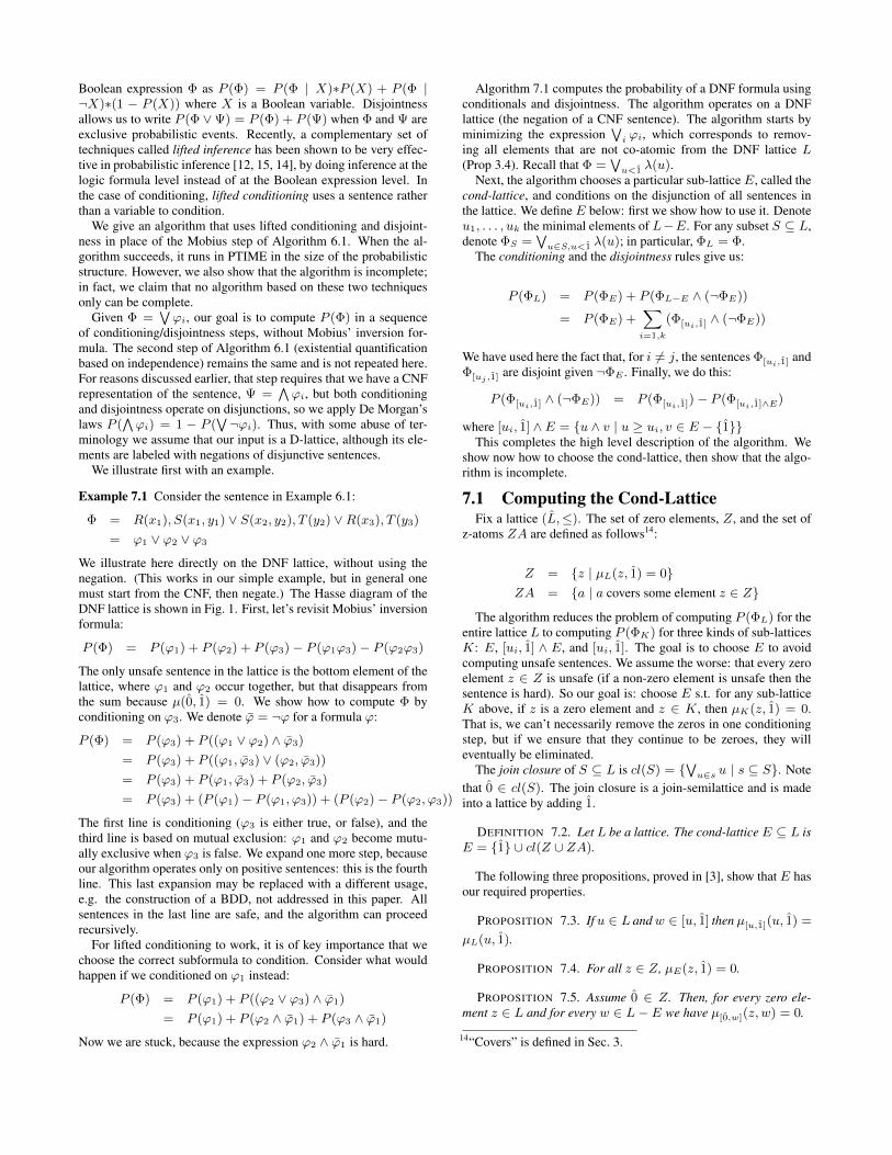
Figure 2: A lattice that is atomic, coatomic, and µ(0̂, 1̂) = 0.Its sentence Φ is given by Th. 6.6 (compare to h3 in Sec. 5.2).

Example 7.6 Consider Example 7.1. The cond-lattice for Fig. 1(a) is

E = cl({0̂, (ϕ1, ϕ3), (ϕ3, ϕ2)})= {0̂, (ϕ1, ϕ3), (ϕ3, ϕ2), ϕ3, 1̂}

Notice that this set is not co-atomic: in other words, when viewedas a sentence, it minimizes to ϕ3, and thus we have gotten rid of 0̂.

To get a better intuition on how conditioning works from a lattice-theoretic perspective, consider the case when Z = {0̂}. In thiscase ZA is the set of atoms, and E is simply the set of all atomicelements; usually this is a strict subset of L, and conditioning parti-tions the lattice intoE, [ui, 1̂]∧E, and [u1, 1̂]. When processingErecursively, the algorithm retains only co-atomic elements. Thus,conditioning works by repeatedly removing elements that are notatomic, then elements that are not co-atomic, until 0̂ is removed,in which case we have removed the unsafe sentence and we canproceed arbitrarily.

7.2 IncompletenessAssume 0̂ is an unsafe sentence, and all other sentences in the

lattice are safe. Lifted conditioning proceeds by repeatedly replac-ing the lattice L with a smaller lattice E, obtained as follows: firstretain only the atomic elements (= cl(Z ∪ ZA)), then retain onlythe co-atomic elements (this is minimization of the resulting for-mula). Conditioning on any formula other than E is a bad idea,because then we get stuck having to evaluate the unsafe formulaat 0̂. Thus, lifted conditioning repeatedly trims the lattice to theatomic-, then to the co-atomic-elements, until, hopefully, 0̂ is re-moved. Proposition 3.4 implies that, if 0̂ is eventually removed thisway, then µ(0̂, 1̂) = 0. But does the converse hold ?

Fig.2 shows a lattice where this process fails. Here µ(0̂, 1̂) =0; by Th. 6.6 there exists a sentence Φ that generates this lattice,where 0̂ is unsafe and all other elements are safe (Φ is shown inthe Figure). Yet the lattice is both atomic and co-atomic. Hencecond-lattice is the entire lattice E = L. We cannot condition onany formula and still have µ(0̂, 1̂) = 0 in the new lattice. In otherwords, no matter what formula we condition on, we will eventuallyget stuck having to evaluate the sentence at 0̂. On the other hand,Mobius’ inversion formula easily computes the probability of thissentence, by exploiting directly the fact that µ(0̂, 1̂) = 0.

8. CONCLUSIONSWe have proposed a simple, yet non-obvious algorithm for com-

puting the probability of an existential, positive sentence over a

Algorithm 7.1 Compute PΦ) using lifted conditionalInput: Φ =

∨i=1,m ϕi, L = LDNF (Φ)

Output P (Φ)

1: Function Cond(L)2: If L has a single co-atom Then proceed with IndepStep3: Remove from L all elements that are not co-atomic (Prop 3.4)4: Let Z = {u | u ∈ L, µL(u, 1̂) = 0}5: Let ZA = {u | u ∈ L, u covers some z ∈ Z}6: If Z = ∅ Then E := [u, 1̂] for arbitrary u7: Else E := cl(Z ∪ ZA)8: If E = L then FAIL (unable to proceed)9: Let u1, . . . , uk be the minimal elements of L− E

10: Return Cond(E)+∑i=1,kCond(ui)−Cond([ui, 1̂]∧E)

probabilistic structure. For every safe sentence, the algorithm runsin PTIME in the size of the input structure; every unsafe sentenceis hard. Our algorithm relies in a critical way on Mobius’ inversionformula, which allows it to avoid attempting to compute the prob-ability of sub-sentences that are hard. We have also discussed thelimitations of an alternative approach to computing probabilities,based on conditioning and independence.

Acknowledgments We thank Christoph Koch and Paul Beamefor pointing us (independently) to incidence algebras, and the anony-mous reviewers for their comments. This work was partially sup-ported by NSF IIS-0713576.

9. REFERENCES[1] N. Creignou and M. Hermann. Complexity of generalized

satisfiability counting problems. Inf. Comput, 125(1):1–12, 1996.[2] Nadia Creignou. A dichotomy theorem for maximum generalized

satisfiability problems. J. Comput. Syst. Sci., 51(3):511–522, 1995.[3] N. Dalvi, K. Schnaitter, and D. Suciu. Computing query probability

with incidence algebras. Technical Report UW-CSE-10-03-02,University of Washington, March 2010.

[4] N. Dalvi and D. Suciu. Efficient query evaluation on probabilisticdatabases. In VLDB, Toronto, Canada, 2004.

[5] N. Dalvi and D. Suciu. The dichotomy of conjunctive queries onprobabilistic structures. In PODS, pages 293–302, 2007.

[6] N. Dalvi and D. Suciu. Management of probabilistic data:Foundations and challenges. In PODS, pages 1–12, Beijing, China,2007. (invited talk).

[7] Adnan Darwiche. A differential approach to inference in bayesiannetworks. Journal of the ACM, 50(3):280–305, 2003.

[8] Erich Grädel, Yuri Gurevich, and Colin Hirsch. The complexity ofquery reliability. In PODS, pages 227–234, 1998.

[9] Kevin H. Knuth. Lattice duality: The origin of probability andentropy. Neurocomputing, 67:245–274, 2005.

[10] Dan Olteanu and Jiewen Huang. Secondary-storage confidencecomputation for conjunctive queries with inequalities. In SIGMOD,pages 389–402, 2009.

[11] Dan Olteanu, Jiewen Huang, and Christoph Koch. Sprout: Lazy vs.eager query plans for tuple-independent probabilistic databases. InICDE, pages 640–651, 2009.

[12] D. Poole. First-order probabilistic inference. In IJCAI, 2003.[13] Yehoushua Sagiv and Mihalis Yannakakis. Equivalences among

relational expressions with the union and difference operators.Journal of the ACM, 27:633–655, 1980.

[14] P. Sen, A.Deshpande, and L. Getoor. Bisimulation-basedapproximate lifted inference. In UAI, 2009.

[15] Parag Singla and Pedro Domingos. Lifted first-order beliefpropagation. In AAAI, pages 1094–1099, 2008.

[16] Richard P. Stanley. Enumerative Combinatorics. CambridgeUniversity Press, 1997.

[17] Ingo Wegener. BDDs–design, analysis, complexity, and applications.Discrete Applied Mathematics, 138(1-2):229–251, 2004.