COMPUTING MOTION IN THE PRIMATE'S VISUAL SYSTEMComputing motion on the basis of the time-varying image intensity is a difficult problem for both artificial and biological vision systems

/. exp. Biol. 146, 115-139 (1989) 115Printed in Great Britain © The Company of Biologists Limited 1989

COMPUTING MOTION IN THE PRIMATE'S VISUAL SYSTEM

BY CHRISTOF KOCHComputation and Neural Systems Program, Divisions of Biology and

Engineering and Applied Sciences, 216-76, California Institute of Technology,Pasadena, CA 91125, USA

H. TAICHI WANG and BIMAL MATHUR

Science Center, Rockwell International, Thousand Oaks, CA 91360, USA

Summary

Computing motion on the basis of the time-varying image intensity is a difficultproblem for both artificial and biological vision systems. We will show how onewell-known gradient-based computer algorithm for estimating visual motion canbe implemented within the primate's visual system. This relaxation algorithmcomputes the optical flow field by minimizing a variational functional of a formcommonly encountered in early vision, and is performed in two steps. In the firststage, local motion is computed, while in the second stage spatial integrationoccurs. Neurons in the second stage represent the optical flow field via apopulation-coding scheme, such that the vector sum of all neurons at each locationcodes for the direction and magnitude of the velocity at that location. Theresulting network maps onto the magnocellular pathway of the primate visualsystem, in particular onto cells in the primary visual cortex (VI) as well as ontocells in the middle temporal area (MT). Our algorithm mimics a number ofpsychophysical phenomena and illusions (perception of coherent plaids, motioncapture, motion coherence) as well as electrophysiological recordings. Thus, asingle unifying principle 'the final optical flow should be as smooth as possible'(except at isolated motion discontinuities) explains a large number of phenomenaand links single-cell behavior with perception and computational theory.

IntroductionOne prominent school of thought holds that information-processing systems,

whether biological or man-made, should follow essentially similar computationalstrategies when solving complex perceptual problems, in spite of their vastlydifferent hardware (Marr, 1982). However, it is not apparent how algorithmsdeveloped for machine vision or robotics can be mapped in a plausible manneronto nervous structures, given their known anatomical and physiological con-straints. In this chapter, we show how one well-known computer algorithm forestimating visual motion can be implemented within the early visual system ofprimates.

The measurement of movement can be divided into multiple stages and may be

PCey words: motion, visual cortex, neuronal network, population coding.

116 C. K O C H , H . T. W A N G AND B. MATHUR

performed in different ways in different biological systems. In the primate visualsystem, motion appears to be measured on the basis of two different systems,termed short-range and long-range processes (Braddick, 1974, 1980). The short-range process analyzes continuous motion, or motion presented discretely but withsmall spatial and temporal displacement from one moment to the next (apparentmotion; in the human fovea both presentations must be within 15min of arc andwith 60-100ms of each other). The long-range system processes larger spatialdisplacements and temporal intervals. A second, conceptually more important,distinction is that the short-range process uses the image intensity, or some filteredversion of image intensity (e.g. filtered via a Laplacian-of-Gaussian or adifference-of-Gaussian operator), to compute motion, while the long-rangeprocess uses more high-level 'token-like' motion primitives, such as lines, corners,triangles etc. (Ullman, 1981). Among short-range motion processes, the two mostpopular classes of algorithms are the gradient method on the one hand (Limb &Murphy, 1975; Fennema & Thompson, 1979; Marr & Ullman, 1981; Hildreth,1984; Yuille & Grzywacz, 1988) and the correlation, second-order or spatio-temporal energy methods on the other hand (Hassenstein & Reichardt, 1956;Poggio & Reichardt, 1973; van Santen & Sperling, 1984; Adelson & Bergen, 1985;Watson & Ahumada, 1985). Gradient methods exploit the relationship betweenthe spatial and the temporal intensity gradient at a given point to estimate localmotion, while the second class of algorithms multiplies a filtered version of theimage intensity with a slightly delayed version of the filtered intensity from aneighboring point (a mathematical operation similar to correlation; hence theirname (for a review, see Hildreth & Koch, 1987).

Computational theory

The problem in computing the optical flow field consists of labeling every pointin a visual image with a vector, indicating at what speed and in what direction thispoint moves (for reviews on motion see Ullman, 1981; Nakayama, 1985; Horn,1986; Hildreth & Koch, 1987). One limiting factor in any system's ability toaccomplish this is the fact that the optical flow, computed from the changing imagebrightness, can differ from the underlying two-dimensional velocity field. Thisvector field, a purely geometrical concept, is obtained by projecting the three-dimensional velocity field associated with moving objects onto the two-dimen-sional image plane. A perfectly featureless rotating sphere will not induce anyoptical flow field, even though the underlying velocity field differs from zeroalmost everywhere. Conversely, if the sphere does not rotate but a light source,such as the sun, moves across the scene the computed optical flow will be differentfrom zero even though the velocity field is not (Horn, 1986). In general, if theobjects in the scene are strongly textured, the optical flow field should be a goodapproximation to the underlying velocity field (Verri & Poggio, 1987).

The basic tenet underlying Horn & Schunck's (1981) analysis of the problem ofcomputing the optical flow field from the time-varying image intensity I(x,y,i%

Computing motion 117

falling onto a retina or a phototransistor array is that the total derivative of theimage intensity between two image frames separated by the interval dr is zero:dl(x,y,t)/dt = 0. In other words, the image intensity seen from the point-of-view ofan observer located in the image plane and moving with the image, does notchange. This conservation law is strictly only satisfied for translation of a rigidLambertian body in planes parallel to the image plan (for a detailed error analysissee Kearney et al. 1987). This law will be violated to some extent for other types ofmovements, such as motion in depth or rotation around an axis. The question is towhat extent this rule will be violated and whether the system built using thishypothesis will suffer from a severe 'visual illusion'.

Using the chain rule of differentiation, dl/dt = 0 can be reformulated asIxx+Iyy+I[ = VI- V+It = 0, where x' = dx/dt and y = dy/dt are the x and ycomponents of velocity V, and Ix = 91/dx, Iy = 31/dy and /, = 91/dt are the spatialand temporal image gradients which can be measured from the image (vectors areprinted in boldface). Formulating the problem in this manner leads to a singleequation in two unknowns x',y. Measuring at n different locations does not help ingeneral, since we are then faced with n linear equations in In unknowns. This typeof problem is termed ill-posed (Hadamard, 1923). One way to make theseproblems well-behaved in a precise, mathematical sense, is to impose additionalconstraints in order to be able to compute unambiguously the optical flow field.The fact that we are unable to measure both components of the velocity vector isalso known as the 'aperture' problem. Any system with a finite viewing apertureand the rule dl/dt = 0 can only measure the component of motion - 7 , / | V/| alongthe spatial gradient V7 = (Ix,Iy). The motion component perpendicular to the localgradient remains invisible. In addition to the aperture problem, the initial motiondata is usually noisy and may be sparse. That is, at those locations where the localvisual contrast is weak or zero, no initial optical flow data exist (the featurelessrotating sphere would be perceived as stationary), thereby complicating the task ofrecovering the optical flow field in a robust manner.

To solve this problem Horn & Schunck (1981) first introduced a 'smoothnessconstraint'. The underlying rationale for this constraint is that nearby points onmoving objects tend to have similar three-dimensional velocities; thus, theprojected velocity field should reflect this fact. Their algorithm finds the opticalflow field which is as compatible as possible with the measured motion com-ponents, and also varies smoothly everywhere in the image. This flow field isdetermined by minimizing a cost functional L:

The term in the first square bracket is nothing but the expansion of d//df (seeJabove) and thus represents local motion, measured along the intensity gradient. In


an ideal world free of noise, dl/dt should be zero; we here impose the conditionthat it should be as small as possible to account for unavoidable noise in the motionmeasurement stage. The terms in the second bracket represent a measure of thesmoothness of the flow field, the parameter A controlling the compromise betweenthe smoothness of the desired solution and its closeness to the data. Thecontribution of this term to L will be zero for a spatially constant flow field -induced by rigid motion in the plane — since all spatial derivatives will be zero. Thesmoothness constraint also stabilizes the solution against the unavoidable noise inthe intensity measurements.

Since L is quadratic in x and y and therefore has a unique minimum, the finalsolution minimizing L will represent a trade-off between faithfulness in the dataand smoothness, depending on a parameter A. The Horn & Schunck (1981)algorithm derives motion at every point in the image by taking into account motionin the surrounding area. It can be shown that it finds the qualitatively correctoptical flow field for real images (for a mathematical analysis in terms of the theoryof dynamic systems see Verri & Poggio, 1987). Such as area-based optical flowmethod is in marked contrast to the edge-based algorithm of Hildreth (1984); sheproposes to solve the aperture problem by computing the optical flow along edges(in her case zero-crossings of the filtered image) using a variational functional verysimilar to that of equation 1.

The use of general constraints (as compared to very specific constraints of thetype 'a red blob at desk-top height is a telephone', popular in early computervision algorithms) is very common to solve the ill-posed problems of early vision(Poggio et al. 1985). Thus, continuity and uniqueness are exploited in the Marr &Poggio (1977) cooperative stereo algorithm, smoothness is used in surfaceinterpolation (Grimson, 1981) and rigidity is used for reconstructing a three-dimensional figure from motion (structure-from-motion; Ullman, 1979).

Before we continue, it is important to emphasize that the optical flow iscomputed in two, conceptually separate, stages. In the first stage, an initialestimate of the local motion, based on spatial and temporal image intensities, iscomputed. Horn & Schunck's method of doing this (using dl/dt = 0) belongs to abroad class of motion algorithms, collectively known as gradient algorithms (Limb& Murphy, 1975; Fermema & Thompson, 1979; Marr & Ullman, 1981; Hildreth,1984; Yuille & Grzywacz, 1988). A new variant of the gradient method, usingdVl/dt = 0 to compute local motion, leads to uniqueness of the optical flow, sincethis constraint is equivalent to two linear independent (in general) equations intwo unknowns (Uras et al. 1988). Thus, in this formulation, computing optical flowis not an ill-posed but an ill-conditioned problem. Alternatively, a correlation orsecond-order model could be used at this stage for estimating local motion(Hassenstein & Reichardt, 1956; Poggio & Reichardt, 1973; van Santen &Sperling, 1984; Adelson & Bergen, 1985; Watson & Ahumada, 1985; Reichardt etal. 1988). However, for both principal (e.g. non-uniqueness of initial motionestimate) and practical (e.g. robustness to noise) reasons, all these methodsrequire a second, independent stage where smoothing occurs.


However, while the optical flow generally varies smoothly from location tolocation, it can change quite abruptly across discontinuities. Thus, the flow fieldassociated with a flying bird varies smoothly across the animal but drops to zero'outside' the bird (since the background is stationary). In these cases of motiondiscontinuities - usually encountered when objects move across each other -smoothing should be prevented (see below and Hutchinson et al. 1988).

The cost functional used to compute motion (equation 1) is a quadraticvariational functional of a type common in early vision (Poggio et al. 1985), andcan be solved using simple electrical networks (Poggio & Koch, 1985). The keyidea is that the power dissipated in a linear electrical network is quadratic in thecurrents or voltages; thus, if the values of the resistances are chosen appropriately,the functional L to be minimized corresponds to power dissipation and the steady-state voltage distribution in the network corresponds to the minimum of L inequation 1. Data are introduced by injecting currents into the nodes of thenetwork. Once the network settles into its steady state - dictated by Kirchhoff s &Ohm's laws - the solution can simply be read off by measuring the voltages atevery node. Efforts are now under way (see, in particular, Luo et al. 1988) to buildsuch resistive networks for various early vision algorithms in the form ofminiaturized circuits using analog, subthreshold CMOS VLSI technology of thetype pioneered by Mead (1989).

Implementation in a neuronal networkWe will now describe a possible neuronal implementation of this computer

vision algorithm. Specifically, we wih1 show that a reformulated variationalfunctional equivalent to equation 1 can be evaluated within the known anatomicaland physiological constraints of the primate visual system and that this formalismcan explain a number of psychophysical and physiological phenomena.

Neurons in the visual cortex of mammals represent the direction of motion in avery different manner from resistive networks, using many neurons per locationsuch that each neuron codes for motion in one particular direction (Fig. 1). In thisrepresentation, the velocity vector V(i,j) [where (/',/) are the image planecoordinates of the center of the cell's receptive field] is not coded explicitly but iscomputed across a population of n such cells, each of which codes for motion in adifferent direction (given by the unit vector ©k), such that:

v(i,j) = I v(t,j,k)ek. (2)

Thus, the cells V(i,j,k) have spatially overlapping receptive fields but withdifferent preferred direction of motion k. This population-coding scheme implies,of course, that all neurons corresponding to location ij represent a single, uniquevalue of velocity, an assumption which breaks down during the perception of two|timuli moving over each other (see the section on motion transparency). This

120 C. KOCH, H. T. WANG AND B. MATHUR

A k+l kk-l k' + l k' k'-l

9

S, T

y

9

-

\

yU, E

Transientchannel

Reunalimages

Sustainedchannel

Area VI

Direction-selectivecells U

AreaMT

Opticalflow

Orientation-selectivecells E

Fig. 1. Computing motion in neuronal networks. (A) Simple scheme of our model.The image / is projected onto the rectangular 64 by 64 retina and sent to the firstprocessing stage via the 5 and T channels. Subsequently, a set of n = 16 ON-OFForientation- and direction-selective (U) cells code local motion in n differentdirections. Neurons with overlapping receptive field positions ij but differentpreferred directions 8 k (indicated by arrows in the upper right-hand side of eachplane) are arranged here in n parallel planes. The ON subfield of one such U cell isshown in Fig. 8A. The output of both E and U cells is relayed to a second set of 64 by 64V cells where the final optical flow is computed. The final optical flow is represented inthis stage, on the basis of a population coding V(l j ) = Z£_1 V(ij,k)Sv, with n = 16.Each cell V(ij,k) in this second stage receives input from cells E and U at location ij aswell as from neighboring V neurons at different spatial locations. (B) Block model of apossible neuronal implementation. The T and 5 streams originate in the retina andenter the primary visual cortex in layer 4C<* and 4C£. The output of VI projects fromlayer 4B to the middle temporal area (MT). We assume that the ON-OFF orientation-and direction-selective neurons E and U are located in VI, and the final optical flow isassumed to be represented by the V units in area MT.

distributed and coarse population-coding scheme is similar to the coding believedto be used in the system controlling eye movements in the mammalian superiorcolliculus (Lee etal. 1988). Detecting the most active neuron at each location(winner-take-all scheme), as in Bulthoff etal. (1989), is not required. To mimicneuronal responses more accurately, the output of all our model neurons is half-wave rectified; in other words, f(x) = x if J C > 0 and 0 if x<0. Thus, when thd|


inhibitory inputs exceed the excitatory ones, the neuron is silent. We then requireat least n = 4 neurons to represent all possible directions of movement. Note thatin this representation the individual components V(i,j,k) are not the projections ofthe velocity field V(i j ) onto the direction ©k (except for n = 4).

Let us now consider a two-stage model for extracting the optical flow field basedon cortical physiology (Fig. 1). Following Marr & Ullman (1981), we assume thatin a pre-processing stage the intensity distribution /(/,/) is projected onto the imageplane and relayed to the first cortical processing stage via two sets of cells:

(i,j) (3)

and

n i J > , ( )

atwhere G is the two-dimensional Gaussian filter (with a2 = 4 pixels; Marr &Hildreth, 1980; Marr & Ullman, 1981). The V2G filter is very similar to thedifference-of-Gaussian or Mexican hat-shaped receptive fields of retinal ganglioncells (Enroth-Cugell & Robson, 1966). This stage then models the filteringperformed by retinal ganglion cells. S and T cells, however, only represent a first-order approximation of the visual transformations occurring in the retina and thelateral geniculate nucleus, because retinal ganglion cells always show sometransient behavior - different from equation 3 - and do not respond instan-taneously, as would be expected from equation 4. However, little would be gainedat this early stage in our understanding of cortical processing by using much moresophisticated cellular models (for such a detailed dynamic description of cat retinalX cells see Victor, 1987).

In the first processing stage, the local motion information (the velocitycomponent along the local spatial gradient) is measured using n ON-OFForientation- and direction-selective cells U{i,j,k), each with preferred directionindicated by the unit vector 0 k (here the V neurons and the U neurons have thesame number of directions and the same preferred directions for the sake ofsimplicity, even though it is not necessary):

™*- (5)

where e is a constant and V^ the spatial derivative along the direction 0 k . Thisderivative is approximated by projecting the convolved image S(i,j) onto a'simple'-type cortical receptive field, consisting of a 1 by 7 pixel positive (ON)subfield next to a 1 by 7 pixel negative (OFF) subfield. Because of the Gaussianconvolution in the S cells, the resulting receptive field has an ON subfield of 3 by9pixels next to an OFF subfield of the same size (Fig. 8A shows such a subfield).Such receptive fields are common in the primary visual cortex of cats and primates(Hubel & Wiesel, 1962). We assume that at each location n such receptive fields,


each with preferred axis given byQk(ke {l...n}) exist. The cell U{i,j,k) respondsoptimally if a bar or grating oriented at right angles to Ok moves in direction Gk.

Our definition of U differs from the standard gradient model U = — T/VkS, byincluding a gain control term, e, such that t/does not diverge if the visual contrastof the stimulus decreases to zero; thus, U-* — TVkS as | V^̂ S| —>• 0. Under theseconditions of small stimulus contrast, our model can be considered a second-ordermodel, similar to the correlation or spatio-temporal energy models (Hassenstein &Reichardt, 1956; Poggio & Reichardt, 1973; Adelson & Bergen, 1985) and theoutput of the U cell is proportional to the product of a transient cell (T) and asustained simple cell with an odd-symmetric receptive field (VkS); thus, theresponse of U is proportional to the magnitude of velocity. For large values ofstimulus contrast, i.e. \VkS\ > e, U-* — T/VkS. Thus, our model of local motiondetection appears to contain aspects of both gradient and second-order methods,depending on the exact experimental conditions (for a further discussion of thisissue, see Koch etal. 1989).

Finally, as an input to our second stage, we also require a set of ON-OFF,orientation-selective but not direction-selective neurons:

) \ . (6)

The absolute value operation (| • |) ensures that these neurons only respond to theamplitude of the spatial gradient, but not to its sign.

We have now progressed from registering and convolving the image in the retinato computing and representing local motion information within the first stage ofour network. In the second processing stage, we determine the final optical flowfield by computing the activity of a second set of cells, V. The state of theseneurons - coding for the final (global) optical flow field - is evaluated byminimizing a reformulated version of the functional in equation 1. The first termexpresses the fact that the final velocity field should be compatible with the initialdata, i.e. with the local velocity component measured along the spatial gradient('velocity constraint line'). In other words, the velocity at location (i,j),V(i,j) = 22 = i V(i,j,k)&k should be compatible with the local motion term U:

U= I [ I V(iJ,k') cos (*' -k)- U(iJ,k) V ET(iJ,k), (7)

where cos (k'—k) represents the cosine of the angle between 0 k ' and 0 k , andE(i,j,k) is the output of an orientation-selective neuron raised to the mth power.This term ensures that the local motion components U(i,j,k) only have aninfluence when there is an appropriately oriented local pattern; in other words, E™prevents velocity terms incompatible with the measured data from contributingsignificantly to Lo. Thus, we require that the neurons E(i,j,k) do not respondsignificantly to directions differing from Ok. If they do, L$ will increasingly containcontributions from other, undesirable, data terms. A large exponent m isadvantageous on computational grounds, since it will lead to a better selection ofthe velocity constraint line. For our model neurons (with a half-width tuning oij|


approximately 60°), m = 2 gave satisfactory responses. Equation 7 directlycorresponds to the first term in the variational functional of Horn & Schunck(1981), equation 1.

The second, smoothing, term in equation 1 can be reformulated in a straightfor-ward manner by replacing the partial derivatives of x and y by their components interms of V(i,j,k) [for instance, the x component of the vector V(i,j) is given byZ* V(i,j,k)cosSk]. This leads to:

x cos(A:' - k)V{i,j,k'). (8)

We are now searching for the neuronal activity level V(i,j,k) that minimizes thefunctional LQ + kL\. Similar to the original Horn & Schunck's functional, equation1, the reformulated variational functional is quadratic in V(i,j,k), so we can findthis state by evolving V(i,j,k) on the basis of the steepest descent rule:

aV(ij,k)_ djLp + XLr)

k)

The contribution from the Lo term to the right-hand side of this equation has theform:

cos(k-k')Em(i,j,k') \U(i,j,k')- £ cos(k'- k")V(i,j,k") , (10),j,k")] ,J

while the contribution from the Lj term has the form:

A I cos(fc - k')[V(i - l,j,k') + V(i + l,j,k') + V(i,j - 1,/c') + V(iJk'

,k')} . (11)

The terms in equations 10 and 11 are all linear in either UOT V. This enables us toview them as the linear synaptic contributions of the U and V neurons towards theactivity of neuron V(iJ,k). The left-hand term of equation 9 can be interpreted as acapacitative term, governing the dynamics of our model neurons. In other words,in evaluating the new activity state of neuron V{i,j,k), we evaluate equations 10and 11 by summing all the contributions from V and U of the same location i,j aswell as neighbouring V neurons and subsequently using a simple numericalintegration routine to compute the new state at time t+At. The appropriatenetwork carrying out these operations is shown schematically in Fig. 1A.

This neuronal implementation converges to the solution of the Horn & Schunckalgorithm as long as the correct constraint line is chosen in equation 7, that is aslong as the Em term is selective enough to suppress velocity terms incompatiblewith the measured data. In the next two sections, we will illustrate the behavior ofthis algorithm by replicating a number of perceptual and electrophysiologicalêxperiments.


Correspondence to cortical anatomy and physiologyThe neuronal network we propose to compute optical flow (Fig. 1) maps

directly onto the primate visual system. Two major visual pathways, the parvo-and the magnocellular, originate in the retina and are perpetuated into highervisual cortical areas. Magnocellular cells appear to be the ones specialized toprocess motion information (for reviews, see Livingstone & Hubel, 1988; DeYoe& van Essen, 1988), since they respond faster and more transiently and are moresensitive to low-contrast stimuli than parvocellular cells. Parvocellular neurons, incontrast, are selective for form and color.

We do not identify our S and T channels with either the parvo- or the magno-pathway since this is not crucial to our model. Furthermore, reversibly blockingeither the magno- or the parvocellular input to cells in the primary cortex leads to adegradation but not to the abolition of orientation- and direction-selectivity(Malpelli et al. 1981). Different from our model, cortical cells therefore appear tocompute the local estimate of motion in either of the two pathways. Our currentmodel does require that one set of cells signals edge information while a secondpopulation is sensitive to temporal changes in intensity (motion or flicker). Weapproximate the spatial receptive field of our retinal neurons using the Laplacian-of-Gaussian operator and the temporal properties of our transient pathway by thefirst derivative. Thus, the response of our U neurons increases linearly withincreasing velocity of the stimulus. This is, of course, an oversimplification andmore realistic filter functions should be used (see above).

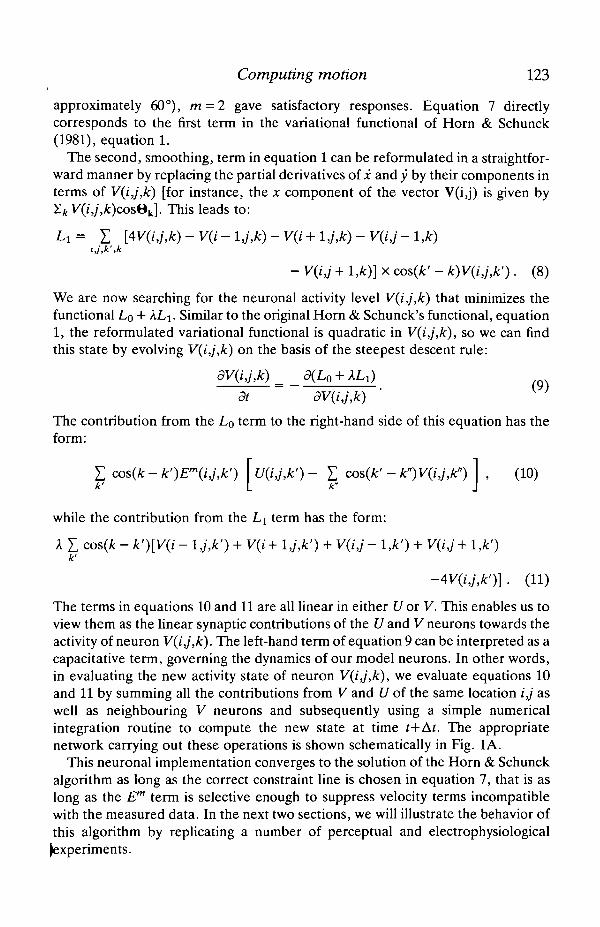
Both the parvo- and the magnocellular pathways project into layer 4C of theprimary visual cortex. Here the two pathways diverge, magnocellular neuronsprojecting to layer 4B (Lund et al. 1976). Cells in this layer are orientation- as wellas direction-selective (Dow, 1974). Layer 4B cells project heavily to a small butwell-defined visual area in the superior temporal sulcus called the middle temporalarea (MT; Allman & Kass, 1971; Baker et al. 1981; Maunsell & van Essen, 1983a).All cells in MT are direction-selective and tuned for the speed of the stimulus; themajority of cells are also orientation-selective. Moreover, irreversible chemicallesions in MT cause striking elevations in psychophysically measured motionthresholds, but have no effect on contrast thresholds (Newsome & Pare, 1988).These findings all support the thesis that area MT is at least partially responsiblefor mediating motion perception. We assume that the orientation- and direction-selective E and U cells corresponding to the first stage of our motion algorithmsare located in layers 4B or 4C in the primary visual cortex or possibly in the inputlayers of area MT, while the V cells are located in the deeper layers of area MT.Inspection of the tuning curve of a V model cell in response to a moving bar revealsits similarity with the superimposed experimentally measured tuning curve of atypical MT cell of the owl monkey (Fig. 2).

The structure of our network is indicated schematically in Fig. 1A. Thestrengths of synapses between the U and the V neurons and among the V neuronsare directly given by the appropriate coefficients in equations 10 and 11. Equation10 contains the contribution from U and E neurons in the primary visual cortex


180°

270°MT neuron

Fig. 2. Polar plot of the median neuron (solid line) in the medial temporal cortex (MT)of the owl monkey in response to a field of random dots moving in different directions(Baker et al. 1981). The tuning curve of one of our model V cells in response to amoving bar is superimposed (dashed line). The distance from the center of the plot isthe average response in spikes per second. Both the cell and its model counterpart aredirection-selective, since motion towards the upper right quadrant evokes a maximalresponse whereas motion towards the lower left quadrant evokes no response. Figurecourtesy of J. Allman and S. Petersen.

well as from MT neurons V at the same location i,j but with differently orientedreceptive fields k'. No spatial convergence or divergence occurs between our Uand V modules, although this could be included. The first part of equation 10 givesthe synaptic strength of the Uto V projection [cos{k-k')Em{i,j,k')U{i,j,k')\. if thepreferred direction of motion of the presynaptic input U(i,j,k') differs by no morethan ±90° from the preferred direction of the postsynaptic neuron V(i,j,k), theU—> V projection will depolarize the postsynaptic membrane. Otherwise, it willact in a hyperpolarizing manner, since the cos(k—k') term will be negative. Noticethat our theory predicts neurons from all cortical orientation columns k' (whichcould be located in either VI or in the superficial layers of MT) projecting onto theVcells, a proposal which could be addressed using anatomical labeling techniques.

The synaptic interaction contains a multiplicative nonlinearity (U-E7"). Thisveto term can be implemented using a number of different biophysical mechan-isms, for instance 'silent' or 'shunting' inhibition (Koch etal. 1982). Thesmoothness term Lx results in synaptic connections among the V neurons, bothamong cells with overlapping receptive fields (same value of i,j) and among cells

Jtvith adjacent receptive fields (e.g. i—l,j). The synaptic strength of these


connections acts in either a de- or a hyperpolarizing manner, depending on thesign of cos(k—k') as well as on their relative locations (see equation 11).

We will next discuss an elegant psychophysical experiment, strongly supportinga two-stage model of motion computation (Adelson & Movshon, 1982; Welch,1989). Moreover, since MT cells in primates, but not cells in VI, appear to mimicthe behavioral response of humans to the psychophysical stimulus, such exper-iments can be used as probes to dissect the different stages in the processing ofperceptual information.

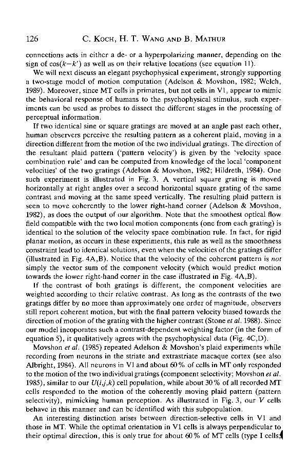
If two identical sine or square gratings are moved at an angle past each other,human observers perceive the resulting pattern as a coherent plaid, moving in adirection different from the motion of the two individual gratings. The direction ofthe resultant plaid pattern ('pattern velocity') is given by the 'velocity spacecombination rule' and can be computed from knowledge of the local 'componentvelocities' of the two gratings (Adelson & Movshon, 1982; Hildreth, 1984). Onesuch experiment is illustrated in Fig. 3. A vertical square grating is movedhorizontally at right angles over a second horizontal square grating of the samecontrast and moving at the same speed vertically. The resulting plaid pattern isseen to move coherently to the lower right-hand corner (Adelson & Movshon,1982), as does the output of our algorithm. Note that the smoothest optical flowfield compatible with the two local motion components (one from each grating) isidentical to the solution of the velocity space combination rule. In fact, for rigidplanar motion, as occurs in these experiments, this rule as well as the smoothnessconstraint lead to identical solutions, even when the velocities of the gratings differ(illustrated in Fig. 4A,B). Notice that the velocity of the coherent pattern is notsimply the vector sum of the component velocity (which would predict motiontowards the lower right-hand corner in the case illustrated in Fig. 4A,B).

If the contrast of both gratings is different, the component velocities areweighted according to their relative contrast. As long as the contrasts of the twogratings differ by no more than approximately one order of magnitude, observersstill report coherent motion, but with the final pattern velocity biased towards thedirection of motion of the grating with the higher contrast (Stone et al. 1988). Sinceour model incoporates such a contrast-dependent weighting factor (in the form ofequation 5), it qualitatively agrees with the psychophysical data (Fig. 4C,D).

Movshon et al. (1985) repeated Adelson & Movshon's plaid experiments whilerecording from neurons in the striate and extrastriate macaque cortex (see alsoAlbright, 1984). All neurons in VI and about 60 % of cells in MT only respondedto the motion of the two individual gratings (component selectivity; Movshon et al.1985), similar to our U(i,j,k) cell population, while about 30 % of all recorded MTcells responded to the motion of the coherently moving plaid pattern (patternselectivity), mimicking human perception. As illustrated in Fig. 3, our V cellsbehave in this manner and can be identified with this subpopulation.

An interesting distinction arises between direction-selective cells in VI andthose in MT. While the optimal orientation in VI cells is always perpendicular totheir optimal direction, this is only true for about 60% of MT cells (type I cells\


V

frt

4

•v

>

V

I. *

\

\

N

N*

N*

N*

\

\

N*

N.Si

s*Si

Si

\

\

\

Si

s*Si

s*Si

\

\

\

\

Si

Si

s.Si

\

\

\

\

\

\

Si

Si

\

\

\

\

\

\

\

\

\

\

\

\

\

\

\

\

\

\

\

\

\

\

\

\

Fig. 3. Mimicking perception and single-cell behavior. (A) Two superimposed squaregratings, oriented orthogonal to each other, and moving at the same speed in thedirection perpendicular to their orientation. The amplitude of the composite is the sumof the amplitude of the individual bars. (B) Response of a patch of 8 by 8 direction-selective simple cells U (outlined in A) to this stimulus. The outputs of all n = 16 cellsare plotted in a radial coordinate system at each location as long as the response issignificantly different from zero; the lengths are proportional to the magnitudes.(C) The output of the V cells using the same needle diagram representation after 2-5time constants. (D) The resulting optical flow field, extracted from C via populationcoding, corresponding to a plaid moving coherently towards the lower right-handcorner, is similar to the perception of human observers (Adelson & Movshon, 1982) aswell as to the response of a subset of MT neurons in the macaque (Movshon et al.1985).

Albright, 1984; Rodman & Albright, 1989). 30% of MT cells respond strongly toflashed bars oriented parallel to their preferred direction of motion (type II cells).These cells also respond best to the pattern motion in the Movshon et al. (1985)^ experiments. Based on this identification, our model predicts that type II


B

>. N* Nl N» î > >i

SWWNS

^ ^ ^ ^ ^ ^ ^

N,

N.

N,

NNN,N.

NNN,

s,NN

Fig. 4. Additional coherent plaid experiments. (A) Two gratings moving towards thelower right (one at —26° and one at —64°), the first moving at twice the speed of thesecond. The final optical flow, coded via the V cells, of a 12 by 12 pixel patch (outlinedin A) is shown in B, corresponding to a coherent plaid moving horizontally towards theright. The final optical flow is within 5% of the correct flow field. (C) Similar to theexperiment illustrated in Fig. 3, except that the contrast of the horizontally orientedgrating only has 75 % of the contrast of the vertically oriented gTating. The final opticalflow (D) is biased towards the direction of motion of the vertical grating, in agreementwith psychophysical experiments (Stone etal. 1988; compare with Fig. 3D).

cells should respond to an extended bar (or grating) moving parallel to its edge.Even though, in this case, no motion information is available if only the classicalreceptive field of the MT cell is considered, motion information from the trailingand leading edges will propagate along the entire bar. Thus, neurons whosereceptive fields are located away from the edges will eventually (i.e. after severaltens of milliseconds) signal motion in the correct direction, even though thedirection of motion is parallel to the local orientation. This neurophysiologicalprediction is illustrated in Fig. 8A,B.

Cells in area MT respond well not only to motion of a bar or gTating but also to amoving random dot pattern (Albright, 1984; Allman etal. 1985), a stimuli!^

Computing motion

B

129

Fig. 5. Figure-ground response. (A) The first frame of two random-dot stimuli. Thearea outlined was moved 1 pixel to the left. (B) The final population-coded velocityfield, signals the presence of a blob, moving towards the left. The outline of thedisplaced area is superimposed onto the final optical flow.

containing no edges or intensity discontinuities. Our algorithm responds well torandom-dot motion, as long as the spatial displacement between two consecutiveframes is not too large (Fig. 5).

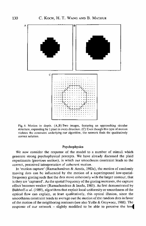
The 'smooth' optical flow algorithms we are discussing only derive the exactvelocity field if a rigid, Lambertian object moves parallel to the image plane. If anobject rotates or moves in depth, the derived optical flow only approximates theunderlying velocity field (Verri & Poggio, 1987). Is this constraint reflected in VIand MT cells? No cells selective for true motion in depth have been reported inprimate VI or MT. Cells in MT do encode information about position in depth,i.e. whether an object is near or far, but not about motion in depth, i.e. whether anobject is approaching or receding (Maunsell & van Essen, 19836). The absence ofcells responding to motion in depth in the primate (but not in the cat; see Cynader& Regan, 1982) supports the thesis that area MT is involved in extracting opticalflow using a smoothness constraint, an approach which breaks down for three-dimensional motion. Cells selective for expanding or contracting patterns, causedby motion in depth, or to rotations of patterns within the frontoparallel plane,were first reported by Saito et al. (1986) in a cortical area surrounding MT, termedthe medial superior temporal area (MST). We illustrate the response of ournetwork to a looming stimuli in Fig. 6. As emphasized previously, our algorithmcomputes the qualitatively correct flow field even in this case when the principalconstraint underlying our analysis, dl/dt = 0, is violated. Since MST receivesheavy fiber projections from MT (Maunsell & van Essen, 1983c), it is likely thatmotion in depth is extracted on the basis of the two-dimensional optical flowômputed in the previous stage.


B

Fig. 6. Motion in depth. (A,B) Two images, featuring an approaching circularstructure, expanding by 1 pixel in every direction. (C) Even though this type of motionviolates the constraint underlying our algorithm, the network finds the qualitativelycorrect solution.

Psychophysics

We now consider the response of the model to a number of stimuli whichgenerate strong psychophysical percepts. We have already discussed the plaidexperiments (previous section), in which our smoothness constraint leads to thecorrect, perceived interpretation of coherent motion.

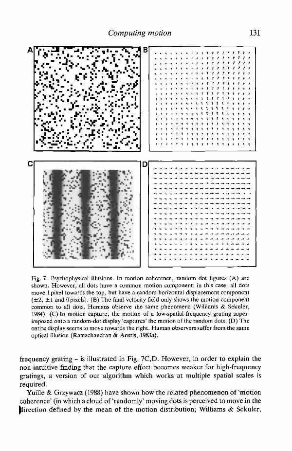
In 'motion capture' (Ramachandran & Anstis, 1983a), the motion of randomlymoving dots can be influenced by the motion of a superimposed low-spatial-frequency grating such that the dots move coherently with the larger contour, thatis they are 'captured'. As the spatial frequency of the grating increases, the captureeffect becomes weaker (Ramachandran & Inada, 1985). As first demonstrated byBiilthoff et al. (1989), algorithms that exploit local uniformity or smoothness of theoptical flow can explain, at least qualitatively, this optical illusion, since thesmoothness constraint tends to average out the motion of the random dots in favorof the motion of the neighboring contours (see also Yuille & Grzywacz, 1988). Theresponse of our network - slightly modified to be able to perceive the ^


Fig. 7. Psychophysical illusions. In motion coherence, random dot figures (A) areshown. However, all dots have a common motion component; in this case, all dotsmove 1 pixel towards the top, but have a random horizontal displacement component(±2, ±1 and Opixels). (B) The final velocity field only shows the motion componentcommon to all dots. Humans observe the same phenomena (Williams & Sekuler,1984). (C) In motion capture, the motion of a low-spatial-frequency grating super-imposed onto a random-dot display 'captures' the motion of the random dots. (D) Theentire display seems to move towards the right. Human observers suffer from the sameoptical illusion (Ramachandran & Anstis, 1983a).

frequency grating - is illustrated in Fig. 7C,D. However, in order to explain thenon-intuitive finding that the capture effect becomes weaker for high-frequencygratings, a version of our algorithm which works at multiple spatial scales isrequired.

Yuille & Grzywacz (1988) have shown how the related phenomenon of 'motioncoherence' (in which a cloud of 'randomly' moving dots is perceived to move in thedirection defined by the mean of the motion distribution; Williams & Sekuler,


1984) can be accounted for using a specific smoothness constraint. Our algorithmalso reproduces this visual illusion quite well (Fig. 7A,B)- In fact, it is surprisinghow often the Gestalt psychologists use the words 'smooth' and 'simple' whendescribing the perceptual organization of objects (for instance in the formulationof the key law of Pragnanz; Kofka, 1935; Kohler, 1969). Thus, one could arguethat these psychologists intuitively captured some of the constraints used in today'scomputer vision algorithms.

Smoothing, that is that the flow field at one location influences motion at adifferent location, will not occur instantaneously. The differential equationimplemented by our network (equations 9-11) can be considered to be a spatialdiscretized version of a parabolic differential equation, a family of partialdifferential equations whose members include the diffusion and the heat equation.We thus expect the time it takes to travel a certain distance to be proportional tothe square of this distance. There exists some psychophysical support for thisnotion. Neighboring flashed dots can impair the speed discrimination of a pair ofbriefly flashed dots in an apparent motion experiment (Bowne & McKee, 1989).This 'motion interference' is time-selective, such that the optimal time ofoccurrence for the stimuli to interfere with the task increases with increasingdistance between the two.

Our algorithm is able to mimic another illusion of the Gestalt psychologists: ymotion (Lindemann, 1922; Kofka, 1931). A figure which is exposed for a shorttime appears with a motion of expansion and disappears with a motion ofcontraction, independent of the sign of contrast. Our algorithm responds in asimilar manner to a flashed disk (Wang etal. 1989). A similar phenomenon haspreviously been reported for both fly and man (Blilthoff & Gotz, 1979). Thisillusion arises from the initial velocity measurement stage and does not rely on thesmoothness constraint.

Our model so far does not take into account temporal integration of velocityinformation over more than two frames [all simulations were always carried outwith only two frames: I{x,y,t) and I(x,y,t + At)]. This is an obvious oversimplifica-tion. From careful psychophysical measurements we know that optimal velocitydiscrimination requires about 80-100 ms (McKee & Welch, 1985). Furthermore, anumber of experiments argue for a 'temporal recruitment' (P. J. Snowden & O. J.Braddick, personal communication) or 'motion inertia' (Ramachandran & Anstis,1983ft) effect, such that the previously perceived velocity or direction of velocityinfluences the currently perceived velocity. Such a phenomenon could bereproduced by including into the variational functional of equation 1 a term whichsmooths over time, such as dV/dl.

Motion transparency

An interesting visual phenomenon is 'motion transparency', in which twoobjects appear to move past or over each other; i.e. at least one object appears tobe transparent. For instance, if the two gratings in the Adelson & Movshon (1982]|


experiment (Fig. 3) differ by an order of magnitude in visual contrast, i.e. onegrating having a strong and the other a weak contrast, or if the two gratings differsignificantly in spatial frequency, they tend not to be perceived as movingcoherently. Perceptually, observers report seeing two gratings sliding past or overeach other. The significant fact is that in these cases, more than one uniquevelocity is associated with a location in visual space.

Welch & Bourne (1989) propose that motion transparency could be decided atthe level of the striate cortex by neurons that compare the local contrast andtemporal frequency content of the moving stimuli. If either of these two quantitiesdiffer substantially - probably caused by two distinct objects - a decision not tocohere would be made. We could then assume within our framework that thisdecision - occurring somewhere prior to our smoothing stage - preventssmoothing from occurring by blocking the appropriate connections among the Vcells with spatially distinct receptive fields. This could be accomplished by settingthe synaptic connection strength to zero either via conventional synaptic inhibitionor via the release of a neurotransmitter or neuropeptide acting over relativelylarge cortical areas. The notion that motion transparency prevents smoothingamong the V cells presupposes that the perceptual apparatus now has access to theindividual motion components V(i,j,k), instead of to the vector sum V(i,j) ofequation 2; only this assumption can explain the perception of two or morevelocity vectors at any one location. Simple electrophysiological experimentscould provide proof for or against our conjecture. For instance, it would be veryintriguing to know how the pattern-selective cells of Movshon et al. (1985) in areaMT respond to the two moving gratings of Adelson & Movshon (1982; see Figs 3and 4). We know that if the gratings cohere, the cells respond to the motion of theplaid. How would these cells respond, however, if the two gratings do not cohereand motion transparency is perceived by the human observer?

Motion discontinuitiesThe major drawback of this and all other motion algorithms is the degree of

smoothness required, smearing out any discontinuities in the flow field, such asthose arising along occluding objects or along a figure-ground boundary. Apowerful idea to deal with this problem was proposed by Geman & Geman (1984;see also Blake & Zisserman, 1987), who introduced the concept of binary lineprocesses which explicitly code for the presence of discontinuities. We adopted thesame approach for discontinuities in the optical flow by introducing binaryhorizontal (lh) and vertical (/*") line processes representing discontinuities in theoptical flow (as first proposed in Koch et al. 1986). If the spatial gradient of theoptical flow between two neighboring points is larger than some threshold,the flow field is 'broken' and the appropriate motion discontinuity at that locationis switched on (/= 1), and no smoothing is carried out. If little spatial variationexists, the discontinuity is switched off (/ = 0). This approach can be justifiedHgorously using Bayesian estimation and Markov random fields (Geman &


Geman, 1984). In our deterministic approximation to their stochastic searchtechnique, a modified version of the variational functional in equation 1 must beminimized (Hutchinson et al. 1988). This functional is, different from before, non-quadratic or non-convex, that is it can have many local minima. Domain-independent constraints about motion discontinuities, such as that they occur ingeneral along extended contours and that they usually coincide with intensitydiscontinuities (edges), are incorporated into this approach (Geman & Geman,1984; Poggio et al. 1988). As before, some of these constraints may be violatedunder laboratory conditions (such as when a homogeneous black figure movesover an equally homogeneous black background and the motion discontinuitiesbetween the figure and the ground do not coincide with the edges, since there areno edges) and the algorithm computes an optical flow field different from theunderlying two-dimensional velocity field (in this case, the computed optical flowfield is zero everywhere). However, for most natural scenes, these motiondiscontinuities lead to a dramatically improved performance of the motionalgorithm (see Hutchinson et al. 1988).

We have not yet implemented motion discontinuities into the neuronal model. Itis known, however, that the visual system uses motion to segment different partsof the scene. Several authors have studied the conditions under which disconti-nuities (in either speed or direction) in motion fields can be detected (Baker &Braddick, 1982; van Doom & Koenderink, 1983; Hildreth, 1984). Van Doom &Koenderink (1983) concluded that perception of motion boundaries requires thatthe magnitude of the velocity difference be larger than some critical value, afinding in agreement with the notion of processes that explicitly code for motionboundaries. Recently, Nakayama & Silverman (1988) studied the spatial interac-tion of motion among moving and stationary waveforms. A number of their resultscould be re-interpreted in terms of our motion discontinuities.

What about the possible cellular correlate of line processes? Allman et al. (1985)first described cells in area MT in the owl monkey whose 'true' receptive fieldextended well beyond the classical receptive field, as mapped with bar or spotstimuli (see Tanaka et al. 1986, for such cells in macaque MT). About 40-50 % ofall MT cells have an antagonistic direction-selective surround, such that theresponse of the cell to motion of a random dot display or an edge within the centerof the receptive field can be modified by moving a stimulus within the surroundingregion that is 50-100 times the area of the center. The response depends on thedifference in speed and direction of motion between the center and the surround,and is maximal if the surround moves at the same speed as the stimulus in thecenter but in the opposite direction. In brief, these cells become activated if amotion discontinuity exists within their receptive field. In cats, similar cells appearat the level of areas 17 and 18 (Orban & Gulyas, 1988). These authors havespeculated as to the existence of two separate cortical systems, one for detectingand computing continuous variables, such as depth or motion, and one fordetecting and handling boundaries. Thus, tantalizing hints exist as to the possibleneuronal basis of motion discontinuities.


f

t4

—

•

• • - . . . ' <

• • • f

. . . , .

' f

• • • « . f . I » 1—. ,. .

• • . <.

S * ' « * • • • • • «

t < «. *

• • • • » • * • • • r

u

Fig. 8. Robustness of the neuronal network. A dark bar (outlined in all images) ismoved parallel to its orientation towards the right. (A) Owing to the apertureproblem, those U neurons whose receptive field only 'see' the straight elongated edgesof the bar - and not a corner - will fail to respond to this moving stimulus, since itremains invisible on the basis of purely local information. The ON subfield of thereceptive field of a vertically oriented U cell is superimposed for comparison. (B) It isonly after information has been integrated, following the smoothing process inherentin the second stage of our algorithm, that the V neurons respond to this motion. TypeII cells of Albright (1984) in MT should respond to this stimulus whereas cells in VI donot. (C) Subsequently, we randomly 'lesion' 25 % of all V neurons, that is, their outputis always set to 0. The resulting distribution of V cells is obviously perturbed.(D) However, given the redundancy build into the V cells (at each location n = 16neurons signal the direction of motion), the final population-coded velocity field onlydiffers on average by 3 % from the flow field computed with no 'damaged' neurons.

Conclusion

The principal contribution of this article is to show how a well-known algorithmfor computing optical flow, based on minimizing a quadratic functional via aRelaxation scheme, can be mapped onto the visual system of primates. ThePbderlying neuronal network uses a population-coding scheme and is very robust


in the face of hardware errors such as missing connections (Fig. 8). While thedetails of our algorithm are bound to be incorrect, it does explain qualitatively anumber of perceptual phenomena and illusions, as well as electrophysiologicalexperiments, on the basis of a single unifying principle: the final optical flowshould be as smooth as possible. We are much less satisfied with our formulation ofthe initial, local stage of motion computation, because the detailed properties ofdirection-selective cortical cells in cat and primates do not agree with those of ourU cells. The challenge here is to bring the biophysics of such motion-detecting cellinto agreement with the well-explored phenomenological theories of psychophy-sics and computational vision (Grzywacz & Koch, 1988; Suarez & Koch, 1989).

The performance of our motion algorithm implemented via resistive grids(Hutchinson et al. 1988) is substantially improved following the introduction ofprocesses which explicitly label for the existence of motion discontinuities, acrosswhich no smoothing should occur. It would be surprising if the nervous system hasnot made use of such an idea.

ReferencesADELSON, E. H. & BERGEN, J. R. (1985). Spatio-temporal energy models for the perception of

motion. /. opt. Soc. Am. A 2, 284-299.ADELSON, E. H. & MOVSHON, J. A. (1982). Phenomenal coherence of moving visual patterns.

Nature, Lond. 200, 523-525.ALBRIGHT, T. L. (1984). Direction and orientation selectivity of neurons in visual are a MT of the

macaque. J. Neurophysiol. 52, 1106-1130.ALLMAN, J. M. &KASS, J. H. (1971). Representation of the visual field in the caudal third of the

middle temporal gyms of the owl monkey (Aotus trivirgatus). Brain Res. 31, 85-105.ALLMAN, J., MIEZIN, F. & MCGUINNESS, E. (1985). Direction- and velocity-specific responses

from beyond the classical receptive field in the middle temporal area (MT). Perception 14,105-126.

BAKER, C. L. & BRADDICK, O. J. (1982). Does segregation of differently moving areas depend onrelative or absolute displacement. Vision Res. 7, 851-856.

BAKER, J. F., PETERSEN, S. E., NEWSOME, W. T. & ALLMAN, J. M. (1981). Visual responseproperties of neurons in four extrastriate visual areas of the owl monkey (Aotus trivirgatus): aquantitative comparison of medial, dorsomedial, dorsolateral and middle temporal areas.J. Neurophysiol. 45, 397-416.

BLAKE, A. & ZISSERMAN, A. (1987). Visual Reconstruction. Cambridge, MA: MTT Press.BOWNE, S. F. & MCKEE, S. P. (1989). Motion interference in speed discrimination. J. opt. Soc.

Am. A (in press).BOLTHOFF, H. H. & GOTZ, K. G. (1979). Analogous motion illusion in man and fly. Nature,

Lond. 278, 636-638.BOLTHOFF, H. H., LITTLE, J. J. & POGGIO, T. (1989). Parallel computation of motion:

computation, psychophysics and physiology. Nature, Lond. (in press).BRADDICK, O. J. (1974). A short-range process in apparent motion. Vision Res. 14, 519-527.BRADDICK, O. J. (1980). Low-level and high-level processes in apparent motion. Phil. Trans. R.

Soc. Ser. B 290, 137-151.CYNADER, M. & REGAN, D. (1982). Neurons in cat visual cortex tuned to the direction of motion

in depth: effect of positional disparity. Vision Res. 22, 967-982.DEYOE, E. A. & VAN ESSEN, D. C. (1988). Concurrent processing streams in monkey visual

cortex. Trends Neurosci. 11, 219-226.Dow, B. M. (1974). Functional classes of cells and their laminar distribution in monkey visuals

cortex. J. Neurophysiol. 37, 927-946.


ENROTH-CUGELL, C. & ROBSON, J. G. (1966). The contrast sensitivity of retinal ganglion cells ofthe cat. /. Physiol, Lond. 187, 517-552.

FENNEMA, C. L. & THOMPSON, W. B. (1979). Velocity determination in scenes containing severalmoving objects. Comput. Graph. Image Proc. 9, 301-315.

GEMAN, S. & GEMAN, D. (1984). Stochastic relaxation, Gibbs distribution and the Bayesianrestoration of images. IEEE Trans. Pattern anal. Machine Intell. 6, 721-741.

GRIMSON, W. E. L. (1981). From Images to Surfaces. Cambridge, MA: MIT Press.GRZVWACZ, N. M. & KOCH, C. (1988). Functional properties of models for direction selectivity

in the retina. Synapse 1, 417-434.HADAMARD, J. (1923). Lectures on the Cauchy Problem in linear Partial Differential Equations.

Yale University Press.HASSENSTEIN, B. & REICHARDT, W. (1956). Systemtheoretische Analyse der Zeit-,

Reihenfolgenund Vorzeichenauswertung bei der Bewegungsperzeption des RiisselkafersChlorophanus. Z. Naturforsch. lib, 513-524.

HILDRETH, E. C. (1984). The Measurement of Visual Motion. Cambridge, MA: MIT Press.HILDRETH, E. C. & KOCH, C. (1987). The analysis of visual motion. A. Rev. Neurosci. 10,

477-533.HORN, B. K. P. (1986). Robotic Vision. Cambridge, MA: MIT Press.HORN, B. K. P. & SCHUNCK, B. G. (1981). Determining optical flow. Artif. Intell. 17, 185-20.HUBEL, D. H. & WIESEL, T. N. (1962). Receptive fields, binocular interactions and functional

architecture in the cat's visual cortex. /. Physiol., Lond. 160, 106-154.HUTCHINSON, J., KOCH, C , LUO, J. & MEAD, C. (1988). Computing motion using analog and

binary resistive networks. IEEE Computer 21, 52-61.KEARNEY, J. K., THOMPSON, W. B. & BOLEY, D. L. (1987). Optical flow estimation: an error

analysis of gradient-based methods with local optimization. IEEE Trans. Pattern anal.Machine Intell. 9, 229-244.

KOCH, C , MARROQUIN, J. & YULLLE, A. L. (1986). Analog neuronal networks in early vision.Proc. natn. Acad. Sci. U.S.A. 83, 4263-4267.

KOCH, C , POGGIO, T. & TORRE, V. (1982). Retinal ganglion cells: a functional interpretation ofdendritic morphology. Phil. Trans. R. Soc. Ser. B 298, 227-264.

KOCH, C .WANG, H. T., MATHUR, B., Hsu, A. &SUAREZ,H. (1989). Computing optical flow inresistive networks and in the primate visual system. In Proceedings of the IEEE Workshop onVisual Motion, pp. 62-73, Irvine, March 20-22, pp. 62-72.

KOFKA, K. (1931). In Handbuch der Normalen und Pathologischen Physiologic, vol. 12 (ed. A.Bethe, G. v. Bergmann, G. Embden & A. EUinger). Berlin: Springer-Verlag.

KOFKA, K. (1935). Principles of Gestalt Psychology. Harcourt: Brace & World.KOHLER, W. (1969). The Task of Gestalt Psychology. Princeton: Princeton University Press.LEE, C , ROHRER, W. H. & SPARKS, D. L. (1988). Population coding of saccadic eye movements

by neurons in the superior colliculus. Nature, Lond. 332, 357-360.LIMB, J. O. & MURPHY, J. A. (1975). Estimating the velocity of moving images in television

signals. Comput. Graph. Image Proc. 4, 311-327.LINDEMANN, E. (1922). Experimentelle Untersuchungen iiber das Entstehen und Vergehen von

Gestalten. Psych. Forsch. 2, 5-60.LIVINGSTONE, M. & HUBEL, D. (1988). Segregation of form, color, movement, and depth:

anatomy, physiology and perception. Science 240, 740-749.LUND, J. S., LUND, R. S., HENDRICKSON, A. E., BUNT, A. H. &FUCHS, A. F. (1976). The origin

of efferent pathways from the primary visual cortex, area 17, of the macaque monkey asshown by retrograde transport of horseradish peroxidase. /. comp. Neurol. 164, 287-304.

Luo, J., KOCH, C. & MEAD, C. (1988). An analog VLSI circuit for two-dimensional surfaceinterpolation. In Proceedings of the IEEE Conference on Neural Information ProcessingSystems. Denver, November 28-30.

MCKEE, S. P. & WELCH, L. (1985). Sequential recruitment in the discrimination of velocity./. opt. Soc. Am. A 2, 243-251.

MALPELLI, J. G., SCHILLER, P. H. & COLBY, C. L. (1981). Response properties of single cells inmonkey striate cortex during reversible inactivation of individual lateral geniculate laminae./. Neurophysiol. 46, 1102-1119.

|4ARR, D. (1982). Vision. San Francisco, CA: Freeman.


MARR, D. & HILDRETH, E. C. (1980). Theory of edge detection. Proc. R. Soc. Ser. B 297,181-217.

MARR, D. & POGGIO, T. (1977). Cooperative computation of stereo disparity. Science 195,283-287.

MARR, D. & ULLMAN, S. (1981). Directional selectivity and its use in early visual processing.Proc. R. Soc. B 211, 151-180.

MAUNSELL, J. H. R. & VAN ESSEN, D. (1983a). Functional properties of neurons in middletemporal visual area of the macaque monkey. I. Selectivity for stimulus direction, speed andorientation. J. Neurophysiol. 49,1127-1147.

MAUNSELL, J. H. R. & VAN ESSEN, D. (19836). Functional properties of neurons in middletemporal visual area of the macaque monkey. II. Binocular interactions and sensitivity tobinocular disparity. J. Neurophysiol. 49, 1148-1167.

MAUNSELL, J. H. R. & VAN ESSEN, D. (1983C). The connections of the middle temporal visualarea (MT) and their relationship to a cortical hierarchy in the macaque monkey. /. Neurosci.3, 2563-2586.

MEAD, C. (1989). Analog VLSI and Neural Systems. Reading, MA: Addison-Wesley.MOVSHON, J. A., ADELSON, E. H., GIZZI, M. S. & NEWSOME, W. T. (1985). The analysis of

moving visual patterns. In Expl Brain Res., Suppl. II, Pattern Recognition Mechanisms (ed.C. Chagas, R. Gattass & C. Gross), pp. 117-151. Heidelberg: Springer-Verlag.

NAKAYAMA, K. (1985). Biological motion processing: a review. Vision Res. 25, 625-660.NAKAYAMA, K. & SILVERMAN, G. H. (1988). The aperture problem. II. Spatial integration of

velocity information along contours. Vision Res. 28, 747-75 .NEWSOME, W. T. & PARE, E. B. (1988). A selective impairment of motion perception following

lesions of the middle temporal visual area (MT). /. Neurosci. 8, 2201-2211.ORBAN, G. A. & GULYAS, B. (1988). Image segregation by motion: cortical mechanisms and

implementation in neural networks. In Neural Computers (ed. R. Eckmiller & Ch. v. d.Malsburg), NATO ASI Series, V. F41, pp. 149-158. Heidelberg: Springer Verlag.

POGGIO, T., GAMBLE, E. B. & LITTLE, J. J. (1988). Parallel integration of visual modules. Science242,337-340.

POGGIO, T. & KOCH, C. (1985). Ill-posed problems in early vision: from computational theory toanalog networks. Proc. R. Soc. B 226, 303-323.

POGGIO, T. & REICHARDT, W. (1973). Considerations on models of movement detection.Kybernetik 13, 223-227.

POGGIO, T., TORRE, V. & KOCH, C. (1985). Computational vision and regularization theory.Nature, Lond. 317, 314-319.

RAMACHANDRAN, V. S. & ANSTIS, S. M. (1983a). Displacement threshold for coherent apparentmotion in random-dot patterns. Vision Res. 12, 1719-1724.

RAMACHANDRAN, V. S. & ANSTIS, S. M. (19836). Extrapolation of motion path in human visualperception. Vision Res. 23, 83-85.

RAMACHANDRAN, V. S. & INADA, V. (1985). Spatial phase and frequency in motion capture ofrandom-dot patterns. Spatial Vision 1, 57-67.

REICHARDT, W., EGELHAAF, M. & SCHLOGEL, R. W. (1988). Movement detectors providesufficient information for local computation of 2-D velocity field. Natunvissenschaften 75,313-315.

RODMAN, H. & ALBRIGHT, T. (1989). Single-unit analysis of pattern-motion selective propertiesin the middle temporal area (MT). Expl Brain Res. (in press).

SAJTO, H., YUKIE, M., TANAKA, K., HIKOSAKA, K., FUKUDA, Y. & IWAI, E. (1986). Integrationof direction signals of image motion in the superior sulcus of the macaque monkey.J. Neurosci. 6, 145-157.

STONE, L. S., MULUGAN, J. B. & WATSON, A. B. (1988). Neural determination of the directionof motion: contrast affects the perceived direction of motion. Neurosci. Abstr. 14, 502.5.

SUAREZ, H. & KOCH, C. (1989). Linking linear threshold units with quadratic models of motionperception. Neural Computation (in press).

TANAKA, K., HIKOSAKA, K., SATTO, H., YUKIE, M., FUKUDA, Y. & IWAI, E. (1986). Analysis oflocal and wide-field movements in the superior temporal visual areas of the macaque monkey.J. Neurosci. 6, 134-144.

ULLMAN, S. (1979). The Interpretation of Visual Motion. Cambridge, MA: MTT Press.


ULLMAN, S. (1981). Analysis of visual motion by biological and computer systems. IEEEComputer 14, 57-69.

URAS, S., GIROSI, F., VERRI, A. & TORRE, V. (1988). A computational approach to motionperception. Biol. Cybernetics 60, 79-87.

VAN DOORN, A. J. & KOENDERINK, J. J. (1983). Detectability of velocity gradients in movingrandom-dot patterns. Vision Res. 23, 799-804.

VAN SANTEN, J. P. H. & SPERLING, G. (1984). A temporal covariance model of motionperception. J. opt. Soc. Am. A 1, 451—473.

VICTOR, J. (1987). The dynamics of the cat retinal X cell centre. /. Physiol, Lond. 386,219-246.VERRI, A. & POGGIO, T. (1987). Against quantitative optical flow. Artif. Intell. Lab. Memo No.

917. Cambridge, MA: MIT Press.WANG, H. T., MATHUR, B. & KOCH, C. (1989). Computing optical flow in the primate visual

system. Neural Computation 1, 92-103.WATSON, A. B. & AHUMADA, A. J. (1985). Model of human visual-motion sensing. J. opt. Soc.

Am. A 2, 322-341.WELCH, L. (1989). The perception of moving plaids reveals two motion-processing stages.

Nature, Lond. 337, 734-736.WELCH, L. & BOURNE, S. F. (1989). Neural rules for combining signals from moving gratings.

Ass. Res. Vision Ophthalmol. 30, 75.WILLIAMS, D. & SEKULER, R. (1984). Coherent global motion percepts from stochastic local

motions. Vision Res. 24, 55-62.YUILLE, A. L. & GRZYWACZ, N. M. (1988). A computational theory for the perception of

coherent visual motion. Nature, Lond. 333, 71-73.

Documents

COMPUTING MOTION IN THE PRIMATE'S VISUAL SYSTEMComputing motion on the basis of the time-varying image intensity is a difficult problem for both artificial and biological vision systems