Draft Copy: July 23, 2009

Computing maximally smooth forward rate curves forcoupon bonds

An iterative piecewise quartic polynomial interpolationmethod

Paul M. Beaumont · Yaniv Jerassy-Etzion

23 July 2009

Abstract We present a simple and fast iterative, linear algorithm for simulta-neously stripping the coupon payments from and smoothing the yield curve ofthe term structure of interest rates. The method minimizes pricing errors, con-strains initial and terminal conditions of the curves and produces maximallysmooth forward rate curves.

Keywords term structure of interest rates · yield curve · coupon stripping ·curve interpolation

1 Introduction

In this paper we present an algorithm to construct maximally smooth forwardrate and discount curves from the term structure of on-the-run U.S. Treasurybills and bonds. The maximum smoothness criterion produces more accurateprices for derivatives such as swaps (Adams 2001) and ensures that no artificialarbitrages will be introduced when using the constructed forward curve forpricing securities beyond those used to construct the curves.

Our method uses a piecewise, quartic polynomial interpolation of the for-ward curve based upon Adams and van Deventer (1994) as corrected by Limand Xiao (2002). Their method, however, works only for zero coupon bonds sowe extend the method to work for coupon bonds by simultaneously strippingthe coupons and interpolating the spot curve. It is critical that these steps bedone simultaneously in order to maintain consistency (Hagan and West 2006).

Paul M. BeaumontDepartment of Economics, Florida State Univeristy, Tallahassee, FL 32306, USAand Faculty of Business and Management, University of Balamand, North Lebanon.Tel.: +1 850 644-7085, Fax: +1 850 644-4535E-mail: beaumont@fsu.edu

Yaniv Jerassy-EtzionDepartment of Economics, Florida State Univeristy, Tallahassee, FL 32306, USA

2

The interpolation step alone can be accomplished with a linear algorithm butthe inclusion of simultaneous stripping leads to a highly nonlinear problem.Our approach relies on an iterated linear algorithm that is simple to imple-ment and very fast to compute while maintaining minimal pricing errors andmaximum smoothness of the interpolated curves. We also correct some minorproblems in Lim and Xiao (2002) related to the terminal conditions of spotand forward rate curves.

Our method computes the smoothest possible forward curve among theclass of polynomials which is shown to be a, fourth-order polynomial con-strained to have continuous second derivatives at all node points. Additionalconstraints fix the initial value f(0) and impose the terminal slope of the for-ward curve to be zero. It is also possible to include other constraints such asnon-negativity of the forward rates if necessary. The coefficients of the polyno-mials are chosen so as to minimize the pricing errors on the observed securities.The spot curve and discount functions are derived from the forward curve asdescribed in Section 2. Details of the algorithm are discussed in Section 3.

The primary complication, and what makes modeling the term structurean interesting problem, is that we only observe prices and yields-to-maturityof a finite set of securities from several different markets including on-the-runand off-the-run treasuries, corporate bonds, LIBORs, SWAP rates, and variousderivatives such as TIGR strips. Each of these markets has its own liquidityand risk characteristics that must be accounted for when constructing thediscount function. Our choice is to use on-the-run treasuries because they arethe most liquid and they have very low and uniform credit risk.

In the U.S. Treasury market we observe zero-coupon Treasury bills of ma-turities one, three, six and twelve months and semi-annual coupon payingTreasury bonds of maturities two, three, five, ten and thirty years. Generallythis list of securities is supplemented with the Federal Funds rate or REPOrates of various maturities such as one day and one week in order to observeyields closer to zero maturity. We add the one-week LIBOR and then use thisand the one month T-Bill rate to interpolate backward to the implied zeromaturity rate yt(0). This approach provides us with a good estimate of thevery short end of the spot curve without having to deal with the high dailyvolatility in overnight REPO rates.

Table 1 presents the yield curve data for July 10, 2008 for the on-the-runU.S. Treasuries. The first column of gives the maturity date of the bill or bondin decimals; the second column gives the annualized coupon rate (paid semi-annually) and is zero for the pure discount bills; the third column gives thequoted prices1; column four gives the yield-to-maturity using the appropriateday count conventions; and the final column reports the Macaulay duration of

1 The quoted prices are dirty prices which is the actual cost of the bond and includes theaccrued interest due to the current bond holder. Some sources quote the clean prices whichdo not include the accrued interest since the previous coupon payment.

3

Table 1 Observed yield curve data for on-the-run U.S. Treasuries on 7/10/2008: maturitydate, Coupon rate, quoted price, yield-to-maturity, and Macaulay duration. The second rowis the one week LIBOR and the first row is the y(0) spot rate implied by backward linearinterpolation.

Maturity Coupon Price Yield Duration

7/10/2008 0 100.00 1.426 07/17/2008 0 99.97 1.435 0.01928/7/2008 0 99.89 1.462 0.0767

10/9/2008 0 99.59 1.670 0.24921/8/2009 0 99.01 2.007 0.49837/2/2009 0 97.90 2.194 0.9774

6/30/2010 2.875 100.88 2.418 1.93156/30/2013 3.375 101.30 3.091 4.62715/15/2018 3.875 100.52 3.811 8.31142/15/2038 4.375 99.28 4.4186 17.0089

each security computed as

D =1P

(n∑i=1

ti C/2(1 + ytm)ti

+tn 100

(1 + ytm)tn

)(1)

where P is the bond price, C/2 is one half of the semi-annually paid coupon,ytm is the yield-to-maturity of the bond, and there are n coupon paymentsplus a face value of 100 paid at maturities ti, i = 1, . . . , n.

From these ten observations we need to compute continuous discount, spotand forward rate functions. The first six securities are zero-coupons so theiryield-to-maturities are already the appropriate spot rates and only interpola-tion between these points is required. The last four securities are coupon bondsso the coupon payments need to be stripped from the cash flows to computethe appropriate spot rates.

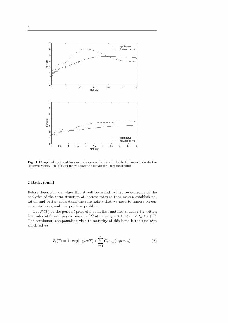
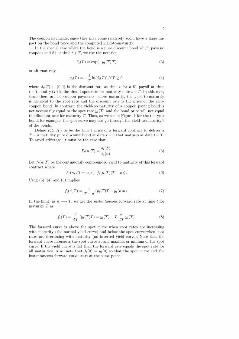
Figure 1 displays the spot curve and instantaneous forward rate curvescomputed by our algorithm for the the data given in Table 1. The spot curveis the solid black line, the instantaneous forward rate curve is the dashed line,and the observed yields are indicated by the small circles. The top figure showsall maturities and the bottom figure zooms in on the short maturities of thecurves.

The figure reveals several important properties of the curves. First, it isclear that the forward curve is much more volatile than the spot curve. This isthe reason that we focus on modeling the forward curve rather than the spotor discount curves. If we can produce a smooth forward curve then we areassured of producing smooth spot and discount curves. The particular termstructure produces a maximum spot rate at about the twenty year maturity soour forward curve intersects the spot curve at that point. Note that the spotand forward curves begin at the same point at the zero maturity date and bothcurves are very stable at long maturities. This latter property is non-trivialand often not observed in polynomial interpolation methods.

4

0 5 10 15 20 25 300

1

2

3

4

5

6

7

Maturity

Perc

ent

spot curveforward curve

0 0.5 1 1.5 2 2.5 3 3.5 4 4.5 50

1

2

3

4

5

6

7

Maturity

Perc

ent

spot curveforward curve

Fig. 1 Computed spot and forward rate curves for data in Table 1. Circles indicate theobserved yields. The bottom figure shows the curves for short maturities.

2 Background

Before describing our algorithm it will be useful to first review some of theanalytics of the term structure of interest rates so that we can establish no-tation and better understand the constraints that we need to impose on ourcurve stripping and interpolation problem.

Let Pt(T ) be the period t price of a bond that matures at time t+T with aface value of $1 and pays a coupon of C at dates ti, t ≤ t1 < · · · < tn ≤ t+ T .The continuous compounding yield-to-maturity of this bond is the rate ytmwhich solves

Pt(T ) = 1 · exp(−ytmT ) +n∑i=1

Ci exp(−ytm ti). (2)

5

The coupon payments, since they may come relatively soon, have a large im-pact on the bond price and the computed yield-to-maturity.

In the special case where the bond is a pure discount bond which pays nocoupons and $1 at time t+ T , we use the notation

δt(T ) = exp(−yt(T )T ) (3)

or alternatively,

yt(T ) = − 1T

ln(δt(T )),∀T ≥ 0, (4)

where δt(T ) ∈ (0, 1] is the discount rate at time t for a $1 payoff at timet+ T , and yt(T ) is the time t spot rate for maturity date t+ T . In this case,since there are no coupon payments before maturity, the yield-to-maturityis identical to the spot rate and the discount rate is the price of the zero-coupon bond. In contrast, the yield-to-maturity of a coupon paying bond isnot necessarily equal to the spot rate yt(T ) and the bond price will not equalthe discount rate for maturity T . Thus, as we see in Figure 1 for the ten-yearbond, for example, the spot curve may not go through the yield-to-maturity’sof the bonds.

Define Ft(n, T ) to be the time t price of a forward contract to deliver aT − n maturity pure discount bond at date t+ n that matures at date t+ T .To avoid arbitrage, it must be the case that

Ft(n, T ) =δt(T )δt(n)

. (5)

Let ft(n, T ) be the continuously compounded yield to maturity of this forwardcontract where

Ft(n, T ) = exp (−ft(n, T )(T − n)) . (6)

Usng (3), (4) and (5) implies

ft(n, T ) =1

T − n(yt(T )T − yt(n)n) . (7)

In the limit, as n −→ T , we get the instantaneous forward rate at time t formaturity T as

ft(T ) =d

d T(yt(T )T ) = yt(T ) + T

d

dTyt(T ). (8)

The forward curve is above the spot curve when spot rates are increasingwith maturity (the normal yield curve) and below the spot curve when spotrates are decreasing with maturity (an inverted yield curve). Note that theforward curve intersects the spot curve at any maxima or minima of the spotcurve. If the yield curve is flat then the forward rate equals the spot rate forall maturities. Also, note that ft(0) = yt(0) so that the spot curve and theinstantaneous forward curve start at the same point.

6

The spot rate yt(T ) is essentially an average of the forward rates up tomaturity T . To see this note that∫ T

0

ft(τ) dτ =∫ T

0

d (τ yt(τ)) = T yt(T ) (9)

or

yt(T ) =1T

∫ T

0

ft(τ) dτ. (10)

Thus, the forward curve is more volatile than the spot curve, which is evidentin our computed curves in Figure 1.

Our task is to find the discount function δt(T ), the spot function yt(T )and the instantaneous forward function ft(T ) for all T ≥ 0 such that they areconsistent with observed market data and satisfy the relationships

δt(T ) = exp(−yt(T )T ) = exp

(−∫ T

0

ft(τ) dτ

)(11a)

ft(T ) = yt(T ) + Td

dTyt(T ) = −

ddT δt(T )δt(T )

(11b)

yt(T ) =1T

∫ T

0

ft(τ) dτ = − 1T

ln δt(T ) (11c)

yt(0) = ft(0). (11d)

It is also reasonable to expect that the spot and forward curves shouldbe well-behaved as maturities increase beyond that of the longest observedsecurity. This is particularly important if we need to price, say, a forwardcontract on a thirty-year bond five or ten years hence. Thus, we assume thatthe spot rate, and therefore the forward rate, approaches a positive asymptote:

limT→∞

yt(T ) = limT→∞

ft(T ) = y∞t . (12)

Again, this property is evident in our curves in Figure 1.Finally, when we model the term structure we assume that current prices

should not permit any arbitrage opportunities among the securities. The no-arbitrage condition implies that the discount function must be monotonicallydecreasing which, in turn, implies that the forward curve must be everywherepositive. We see from Figure 1 that our forward curves satisfy the no-arbitragecondition.

3 Iterative Piecewise Quartic Polynomial Interpolation Algorithm

Our goal is a simple and fast algorithm to compute the forward, spot and dis-count rates associated with the current on-the-run Treasury yield curve. Themethod of Adams and van Deventer (1994) and Lim and Xiao (2002) is linearin the unknown coefficients but only when all securities are zero coupon bonds.

7

As we will see, when coupon bonds are introduced the algorithm becomes non-linear. Our approach is to modify the Lim and Xiao (2002) algorithm and dealwith the nonlinearity by iterating over a sequence of linear problems. Com-pared to other nonlinear algorithms, such as Manzano and Blomvall (2004)and Hagan and West (2006), our approach is simple to code, fast and verystable.

To make the description of the algorithm as concrete as possible we willrefer to the specific data from Table 1 where there are nine observed securitiesin the yield curve plus the initial condition on the settlement date. The firstfive securities are zero coupon bonds with maturities from seven days to aboutone year. The last four securities are the coupon paying bonds with maturitiesbetween two and thirty years.

We will denote the maturities of the securities as Ti, i = 1, . . . ,m andthe price of the bond with maturity Ti as P (Ti). The yield-to-maturities arecomputed according to the appropriate day count conventions for the specificbills and bonds. To simplify our presentation we will use yields based uponcontinuous compounding with actual day counts.

A bond is just a sequence of cash flows on specific days. In our examplethere are 10,812 days between the settlement date of July 10, 2008 and thematurity of the thirty year bond on February 15, 2038. Let Z(Ti) denote the10,812 element cash flow vector for the bond maturing at date Ti. For our firstfive securities, the zero coupons, Z(Ti) will contain all zeros except for the valueof $100 at day Ti. For example, Z(T3) contains $100 in the 91st element—thedays to maturity of the three month T-Bill maturing on October 9, 2008.The cash flow vector for bonds includes the semi-annual coupon payments aswell as the final face value payment. For example, the two year 2.875 couponbond maturing on June 30, 2010 has cash flows of $2.875/2 = $1.4375 on days{174, 355, 539} and a cash flow of $101.4375 on maturity day 720.

Using the notation from Section 2, let δ, y and f be the discount rate, spotrate and instantaneous forward rate functions to be computed. Our methodcomputes the forward curve as a , piecewise, quartic polynomial function andthen derives the spot curve and discount function from it. Given estimates ofthese functions, we could compute the price for each security as

P (Ti) = δ′ Z(Ti), i = 1, . . . ,m, (13)

where δ is the 10,812 element vector of discount rates computed from theforward function f .

The smoothest function is the one that has the minimum acceleration orsmallest absolute second derivatives over its range. A straight line is verysmooth but would not be a good choice for the forward curve because it wouldcreate large pricing errors. The optimization problem is

minf

∫ Tm

0

(f ′′(t))2 dt (14)

subject to the pricing constraints P (Ti) = P (Ti), i = 1, . . . ,m, the initialcondition f(0) = y(0) (= 1.426 in our example) and the terminal condition

8

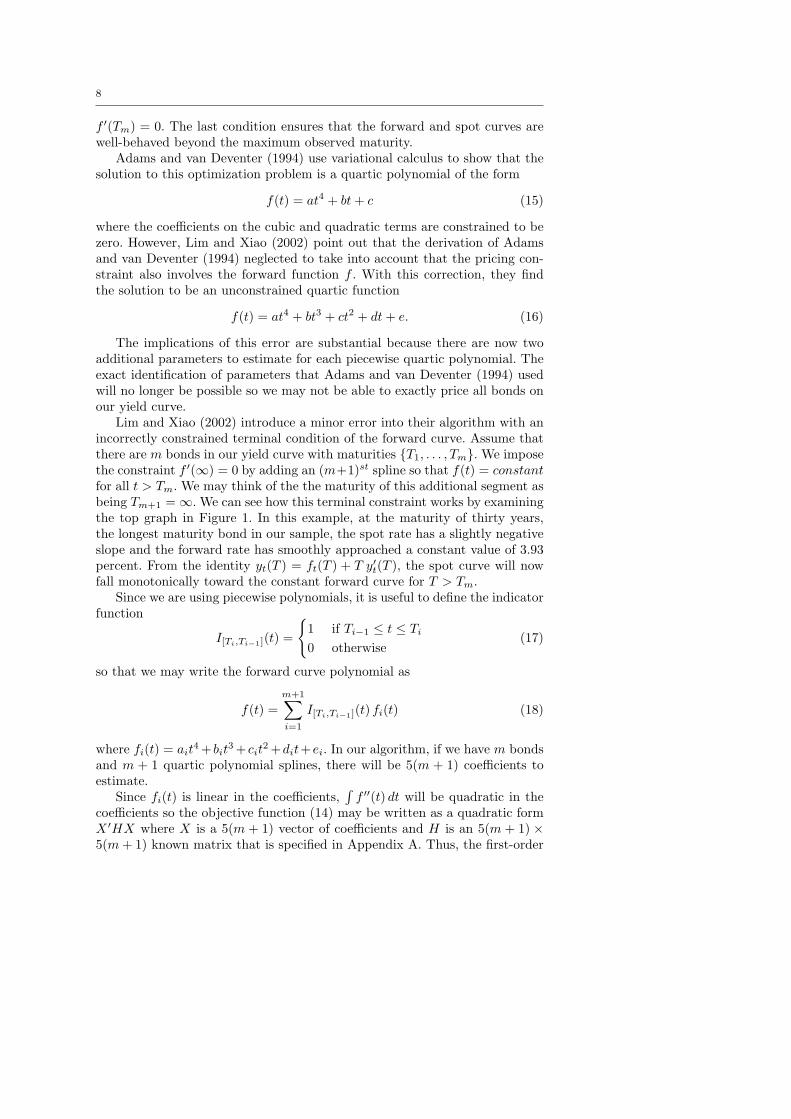
f ′(Tm) = 0. The last condition ensures that the forward and spot curves arewell-behaved beyond the maximum observed maturity.

Adams and van Deventer (1994) use variational calculus to show that thesolution to this optimization problem is a quartic polynomial of the form

f(t) = at4 + bt+ c (15)

where the coefficients on the cubic and quadratic terms are constrained to bezero. However, Lim and Xiao (2002) point out that the derivation of Adamsand van Deventer (1994) neglected to take into account that the pricing con-straint also involves the forward function f . With this correction, they findthe solution to be an unconstrained quartic function

f(t) = at4 + bt3 + ct2 + dt+ e. (16)

The implications of this error are substantial because there are now twoadditional parameters to estimate for each piecewise quartic polynomial. Theexact identification of parameters that Adams and van Deventer (1994) usedwill no longer be possible so we may not be able to exactly price all bonds onour yield curve.

Lim and Xiao (2002) introduce a minor error into their algorithm with anincorrectly constrained terminal condition of the forward curve. Assume thatthere are m bonds in our yield curve with maturities {T1, . . . , Tm}. We imposethe constraint f ′(∞) = 0 by adding an (m+1)st spline so that f(t) = constantfor all t > Tm. We may think of the the maturity of this additional segment asbeing Tm+1 =∞. We can see how this terminal constraint works by examiningthe top graph in Figure 1. In this example, at the maturity of thirty years,the longest maturity bond in our sample, the spot rate has a slightly negativeslope and the forward rate has smoothly approached a constant value of 3.93percent. From the identity yt(T ) = ft(T ) + T y′t(T ), the spot curve will nowfall monotonically toward the constant forward curve for T > Tm.

Since we are using piecewise polynomials, it is useful to define the indicatorfunction

I[Ti,Ti−1](t) =

{1 if Ti−1 ≤ t ≤ Ti0 otherwise

(17)

so that we may write the forward curve polynomial as

f(t) =m+1∑i=1

I[Ti,Ti−1](t) fi(t) (18)

where fi(t) = ait4 + bit

3 + cit2 +dit+ei. In our algorithm, if we have m bonds

and m + 1 quartic polynomial splines, there will be 5(m + 1) coefficients toestimate.

Since fi(t) is linear in the coefficients,∫f ′′(t) dt will be quadratic in the

coefficients so the objective function (14) may be written as a quadratic formX ′HX where X is a 5(m + 1) vector of coefficients and H is an 5(m + 1) ×5(m+ 1) known matrix that is specified in Appendix A. Thus, the first-order

9

conditions with respect to the coefficient vector X will be linear in the un-knowns.

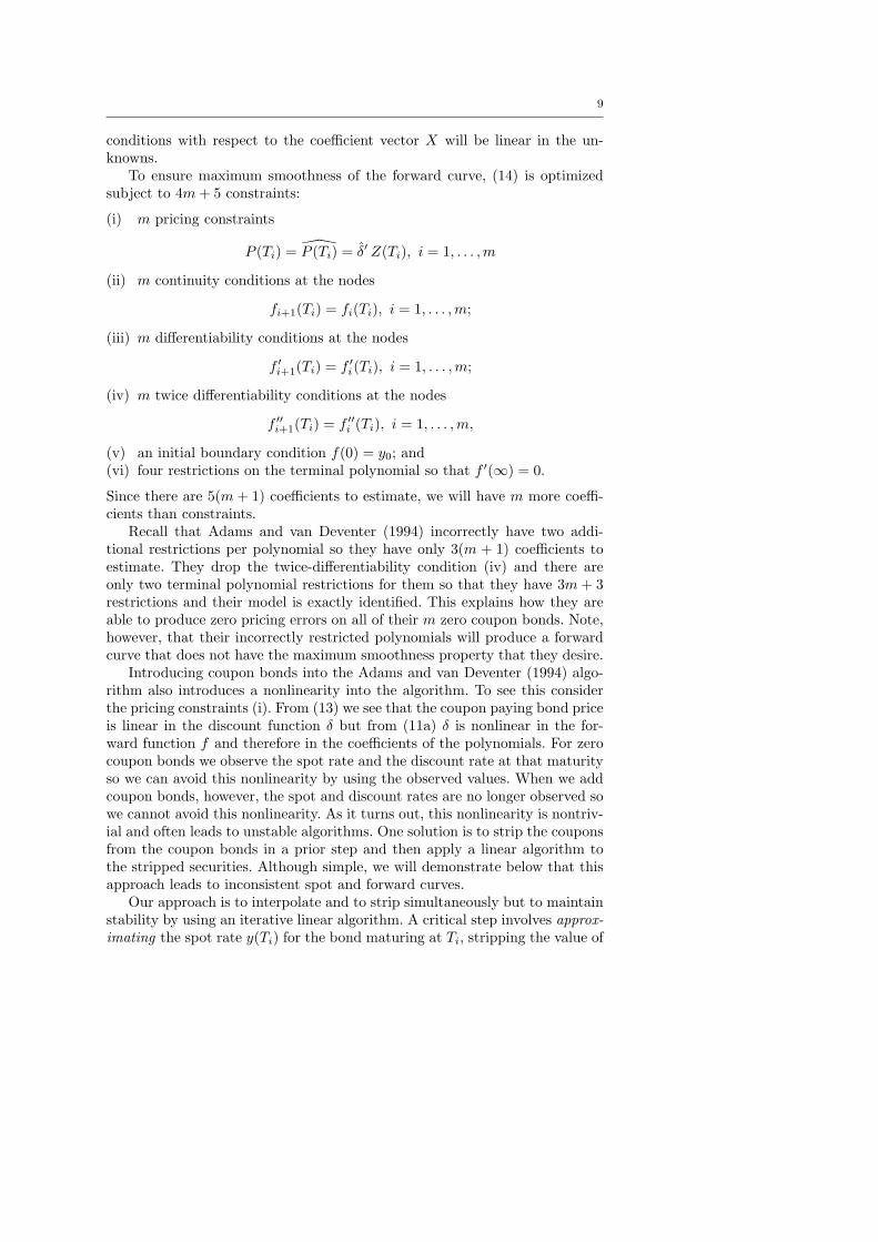
To ensure maximum smoothness of the forward curve, (14) is optimizedsubject to 4m+ 5 constraints:

(i) m pricing constraints

P (Ti) = P (Ti) = δ′ Z(Ti), i = 1, . . . ,m

(ii) m continuity conditions at the nodes

fi+1(Ti) = fi(Ti), i = 1, . . . ,m;

(iii) m differentiability conditions at the nodes

f ′i+1(Ti) = f ′i(Ti), i = 1, . . . ,m;

(iv) m twice differentiability conditions at the nodes

f ′′i+1(Ti) = f ′′i (Ti), i = 1, . . . ,m,

(v) an initial boundary condition f(0) = y0; and(vi) four restrictions on the terminal polynomial so that f ′(∞) = 0.

Since there are 5(m + 1) coefficients to estimate, we will have m more coeffi-cients than constraints.

Recall that Adams and van Deventer (1994) incorrectly have two addi-tional restrictions per polynomial so they have only 3(m + 1) coefficients toestimate. They drop the twice-differentiability condition (iv) and there areonly two terminal polynomial restrictions for them so that they have 3m + 3restrictions and their model is exactly identified. This explains how they areable to produce zero pricing errors on all of their m zero coupon bonds. Note,however, that their incorrectly restricted polynomials will produce a forwardcurve that does not have the maximum smoothness property that they desire.

Introducing coupon bonds into the Adams and van Deventer (1994) algo-rithm also introduces a nonlinearity into the algorithm. To see this considerthe pricing constraints (i). From (13) we see that the coupon paying bond priceis linear in the discount function δ but from (11a) δ is nonlinear in the for-ward function f and therefore in the coefficients of the polynomials. For zerocoupon bonds we observe the spot rate and the discount rate at that maturityso we can avoid this nonlinearity by using the observed values. When we addcoupon bonds, however, the spot and discount rates are no longer observed sowe cannot avoid this nonlinearity. As it turns out, this nonlinearity is nontriv-ial and often leads to unstable algorithms. One solution is to strip the couponsfrom the coupon bonds in a prior step and then apply a linear algorithm tothe stripped securities. Although simple, we will demonstrate below that thisapproach leads to inconsistent spot and forward curves.

Our approach is to interpolate and to strip simultaneously but to maintainstability by using an iterative linear algorithm. A critical step involves approx-imating the spot rate y(Ti) for the bond maturing at Ti, stripping the value of

10

the coupon payments from the bond and then pricing the bond face value usingthe zero-coupon bond price given by (11a) so that the log of the zero couponbond price is linear in the polynomial coefficients. We may then solve ournonlinear optimization problem using a sequence of linear steps. The detailsof the linear steps of the piecewise quartic polynomial interpolation (PQPI)algorithm are similar to those of Lim and Xiao (2002) and are described inthe Appendix A along with our corrections for the terminal conditions. In thenext section we describe the iterative algorithm.

3.1 The Iterative Algorithm

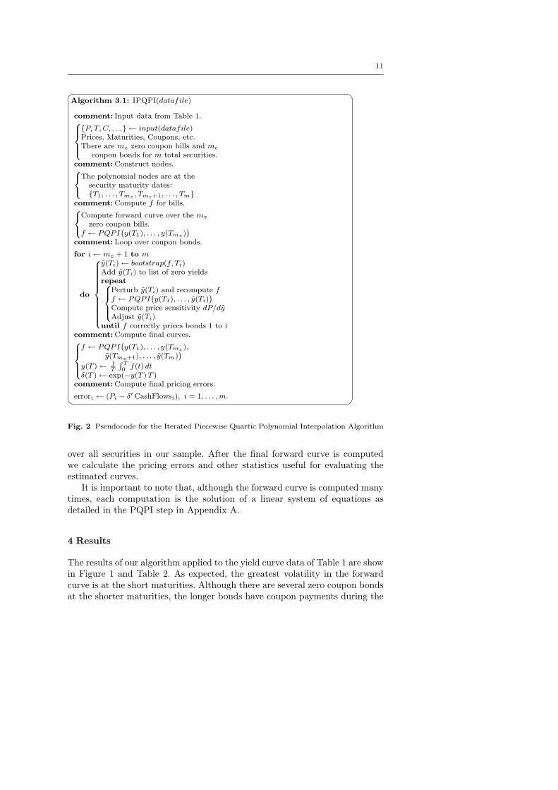
Pseudocode for the main iterative algorithm is shown in Figure 3.1. Afterreading the yield curve data from Table 1 and storing the vector of nodepoints, we first compute the forward curve over the observed zero couponbills. In our example this includes the first five securities up to maturity July2, 2009. Since these are all zero coupon bills we can do this with a slightlymodified version of the linear Lim and Xiao (2002) PQPI algorithm.

Next we add the first coupon bond, the sixth security or the two year 2.875coupon bond maturing on June 30, 2010, to our list of securities. The yieldof 2.418% for this bond includes the coupon payments so we must strip thecoupons and compute the spot rate, y(T6) at this maturity date T6. We dothis by first getting an initial estimate of y(T6) using a simple linear bootstrapmethod. Using this estimated value, we use PQPI to compute an estimateof the forward curve f up through maturity T6. Using f we compute theestimated price P (T6) of the two year bond. This method will not produce anestimate that is consistent with the interpolation up to Ti−1 from the previousstep since some of the coupon payments of the two year bond will occur beforeTi−1, T5, in our example.

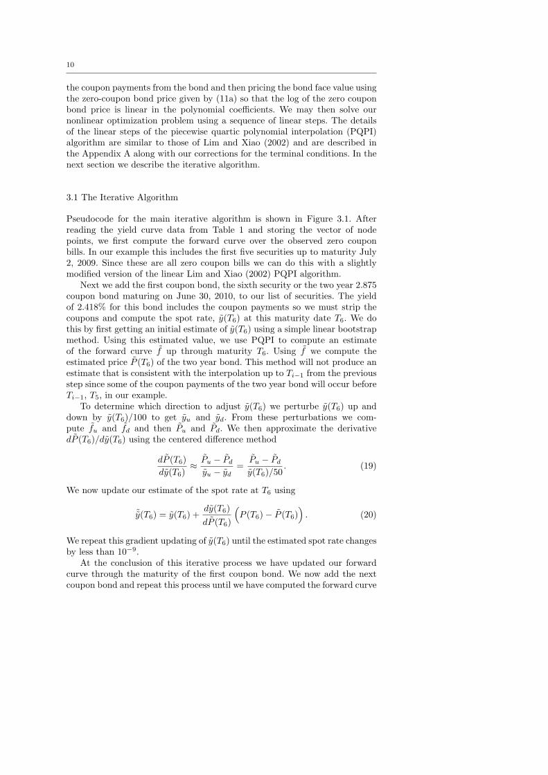
To determine which direction to adjust y(T6) we perturbe y(T6) up anddown by y(T6)/100 to get yu and yd. From these perturbations we com-pute fu and fd and then Pu and Pd. We then approximate the derivativedP (T6)/dy(T6) using the centered difference method

dP (T6)dy(T6)

≈ Pu − Pdyu − yd

=Pu − Pdy(T6)/50

. (19)

We now update our estimate of the spot rate at T6 using

˜y(T6) = y(T6) +dy(T6)dP (T6)

(P (T6)− P (T6)

). (20)

We repeat this gradient updating of y(T6) until the estimated spot rate changesby less than 10−9.

At the conclusion of this iterative process we have updated our forwardcurve through the maturity of the first coupon bond. We now add the nextcoupon bond and repeat this process until we have computed the forward curve

11

�

�

Algorithm 3.1: IPQPI(datafile)

comment: Input data from Table 1.8>><>>:{P, T,C, . . . } ← input(datafile)Prices, Maturities, Coupons, etc.There are mz zero coupon bills and mc

coupon bonds for m total securities.comment: Construct nodes.8<:The polynomial nodes are at the

security maturity dates:{T1, . . . , Tmz , Tmz+1, . . . , Tm}

comment: Compute f for bills.8<:Compute forward curve over the mz

zero coupon bills.f ← PQPI

`y(T1), . . . , y(Tmz )

´comment: Loop over coupon bonds.

for i← mz + 1 to m

do

8>>>>>>>>><>>>>>>>>>:

y(Ti)← bootstrap(f, Ti)Add y(Ti) to list of zero yieldsrepeat8>><>>:

Perturb y(Ti) and recompute ff ← PQPI

`y(T1), . . . , y(Ti)

´Compute price sensitivity dP/dyAdjust y(Ti)

until f correctly prices bonds 1 to icomment: Compute final curves.8>><>>:f ← PQPI

`y(T1), . . . , y(Tmz ),

y(Tmz+1), . . . , y(Tm)´

y(T )← 1T

R T0 f(t) dt

δ(T )← exp(−y(T )T )comment: Compute final pricing errors.

errori ← (Pi − δ′ CashFlowsi), i = 1, . . . ,m.

Fig. 2 Pseudocode for the Iterated Piecewise Quartic Polynomial Interpolation Algorithm

over all securities in our sample. After the final forward curve is computedwe calculate the pricing errors and other statistics useful for evaluating theestimated curves.

It is important to note that, although the forward curve is computed manytimes, each computation is the solution of a linear system of equations asdetailed in the PQPI step in Appendix A.

4 Results

The results of our algorithm applied to the yield curve data of Table 1 are showin Figure 1 and Table 2. As expected, the greatest volatility in the forwardcurve is at the short maturities. Although there are several zero coupon bondsat the shorter maturities, the longer bonds have coupon payments during the

12

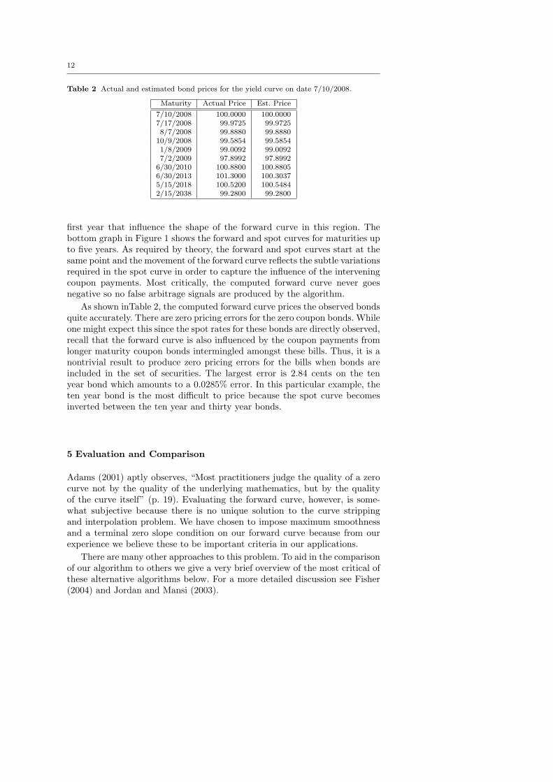
Table 2 Actual and estimated bond prices for the yield curve on date 7/10/2008.

Maturity Actual Price Est. Price

7/10/2008 100.0000 100.00007/17/2008 99.9725 99.97258/7/2008 99.8880 99.8880

10/9/2008 99.5854 99.58541/8/2009 99.0092 99.00927/2/2009 97.8992 97.8992

6/30/2010 100.8800 100.88056/30/2013 101.3000 100.30375/15/2018 100.5200 100.54842/15/2038 99.2800 99.2800

first year that influence the shape of the forward curve in this region. Thebottom graph in Figure 1 shows the forward and spot curves for maturities upto five years. As required by theory, the forward and spot curves start at thesame point and the movement of the forward curve reflects the subtle variationsrequired in the spot curve in order to capture the influence of the interveningcoupon payments. Most critically, the computed forward curve never goesnegative so no false arbitrage signals are produced by the algorithm.

As shown inTable 2, the computed forward curve prices the observed bondsquite accurately. There are zero pricing errors for the zero coupon bonds. Whileone might expect this since the spot rates for these bonds are directly observed,recall that the forward curve is also influenced by the coupon payments fromlonger maturity coupon bonds intermingled amongst these bills. Thus, it is anontrivial result to produce zero pricing errors for the bills when bonds areincluded in the set of securities. The largest error is 2.84 cents on the tenyear bond which amounts to a 0.0285% error. In this particular example, theten year bond is the most difficult to price because the spot curve becomesinverted between the ten year and thirty year bonds.

5 Evaluation and Comparison

Adams (2001) aptly observes, “Most practitioners judge the quality of a zerocurve not by the quality of the underlying mathematics, but by the qualityof the curve itself” (p. 19). Evaluating the forward curve, however, is some-what subjective because there is no unique solution to the curve strippingand interpolation problem. We have chosen to impose maximum smoothnessand a terminal zero slope condition on our forward curve because from ourexperience we believe these to be important criteria in our applications.

There are many other approaches to this problem. To aid in the comparisonof our algorithm to others we give a very brief overview of the most critical ofthese alternative algorithms below. For a more detailed discussion see Fisher(2004) and Jordan and Mansi (2003).

13

5.1 Alternative Algorithms

Early approaches (McCulloch 1971, 1975; Vasicek and Fong 1982) used polyno-mial or exponential splines to fit the discount function directly. One advantageof these approachs is that the polynomials offer enough degrees of freedom sothat the security prices can be fit with minimal error. The problems are two-fold. First, you must already know the discount rate for long maturity bondsand these are not directly observed. Second, as can be seen from (11b), evena very smooth appearing discount function may create erratic forward ratecurves. In the extreme case, if the splines in the discount function are not dif-ferentiable at the nodes then the forward rate curve will have discontinuitiesat those points implying arbitrage opportunities for derivative securities thatare, in fact, merely an artifact of the interpolation algorithm.

Probably the most widely used yield curve model at present is that ofNelson and Siegel (1987) along with the extension of Svensson (1995). Jordanand Mansi (2003) conclude that these are the best models and Gimeno andNave (2006) report that nine out of the thirteen central banks that report theirestimation methods to the Bank of International Settlements, use the Svenssonaugmented version of the Nelson-Siegel model. Consequently, we will reviewthese methods in detail and use them as benchmarks against which we cancompare our model.

Nelson and Siegel (1987) observe that the yield curve generally followsrather simple monotone increasing concave or occasionally humped or evenS-shapes curves. To match this fact they propose a global approach that fitsa specific functional form for the forward rate curve

ft(T ) = β0 + β1 exp(−Tτ

)+ β2

[T

τexp

(−Tτ

)](21)

which, using (11c) gives the spot curve

yt(T ) =β0 + β1

[1− exp

(−Tτ

)Tτ

]

+ β2

([1− exp

(−Tτ

)Tτ

]− exp

(−Tτ

)).

(22)

The first term, the constant β0, is interpreted as the long run level of interestrates, the second term is interpreted as a short-term component that deter-mines the slope of the spot curve for short maturities, and the third term isinterpreted as a medium term component that can capture a hump or dip inthe spot curve. The coefficients are estimated by minimizing the pricing errorsfor the observed securities and we expect β0 > 0, β0 + β1 > 0 and τ > 0.

The Nelson-Siegel functional form has been widely adopted because it hasseveral appealing features. The spot and forward curves are always smoothand continuously differentiable. As the maturity increases we get

limT→∞

yt(T ) = limT→∞

ft(T ) = β0 (23)

14

so that the curves are well-behaved in the limit—a property not always ob-served in polynomial models of the term structure. Note that, in the limit, thespot curve becomes a flat function so the forward curve will asymptoticallyapproach the fixed limiting spot rate.

At the short-end of the term structure we get

limT→0

yt(T ) = limT→0

ft(T ) = β0 + β1 (24)

so the constraint that the forward and spot curves begin at the same point issatisfied. For a normal yield curve that is an upward sloping concave functionwe would expect to find β1 < 0.

One short-coming of the Nelson-Siegel model is that, with only four freeparameters, the model cannot be calibrated to fit all current security pricesand in some cases the pricing errors can be substantial. To improve this aspectof the model, Svensson (1995) added an additional term to the forward curveto get

ft(T ) = β0 + β1 exp(− Tτ1

)+ β2

[T

τ1exp

(−Tτ1

)]+ β3

[T

τ2exp

(−Tτ2

)] (25)

which yields the spot curve

yt(T ) =β0 + β1

1− exp(− Tτ1

)Tτ1

+ β2

1− exp(− Tτ1

)Tτ1

− exp(− Tτ1

)+ β3

1− exp(− Tτ2

)Tτ2

− exp(− Tτ2

) .

(26)

The additional term allows more flexibility in the shapes of the forward andspot curves and the model is easier to calibrate to securities prices since it hassix free parameters.

There are many variations of the Nelson and Siegel (1987) model, includingDiebold and Li (2006) who make a natural and powerful extension by allowingthe parameters to vary over time. The additional degrees of freedom improvethe calibration properties of their model at the cost of additional complexityin modeling the factors that drive the coefficient movements.

Other sophisticated nonlinear approaches include the monotone convexspline method of Hagan and West (2006) and the nonlinear dynamic program-ming method of Manzano and Blomvall (2004). These methods, while verypromising, are highly nonlinear and difficult to implement. Our goal is to pro-vide an easily implemented algorithm that is superior to the most commonlyused algorithms in practice.

15

5.2 Comparison of Algorithms

We will compare our IPQPI method to four alternative methods:

LBLI A simple linear bootstrap and linear interpolation method appliedto the spot curve.

LBPQPI A linear bootstrap method on the spot rates of the coupons with apiecewise quartic polynomial interpolation through these rates.

NS The Nelson-Siegel method described in 5.1.SV The Svensson extension of Nelson-Siegel described in 5.1.

The linear bootstrap with linear interpolation (LBLI) method is simply apiecewise linear interpolation of the spot curve using a bootstrap method tocompute the spot rates at each node. This is straightforward for zero couponbonds when the the spot rates at those maturities are directly observed. Forbonds, we add one bond at a time and adjust the estimated spot rate upor down until that bond is correctly priced. Note that the linear segmentsdetermined in prior steps are not adjusted during this process. The resultingspot curve will be continuous but not differentiable at the node points. Thismethod is admittedly a “straw man” but it is useful for illustrating someimportant features of the IPQPI method.

The LBPQPI method computes the spot rates at the maturities of thebonds in the same way as LBLI except, in the final step, we use a piecewisequartic polynomial interpolation of the computed spot rates to estimate theforward curve. This approach separates the interpolation and stripping stepsand is the most straightforward extension of the various methods, includingthe Lim and Xiao (2002) method, applied to coupon bonds but that requirespot rates as inputs.

The Nelson-Siegel (NS) and Svensson (SV) methods are described in 5.1and, due to their widespread use, are the most serious contenders for ourIPQPI method.

Table 3 reports the pricing errors of the five algorithms for each of secu-rities as well as some summary statistics to evaluate the methods. The firsttwo columns give the maturities and actual prices of the on-the-run treasuriesfor the yield curve on July 10, 2008. The first six securities (including thesettlement date in the first row) are zero coupon bills and the last four secu-rities are the coupon bonds. Columns three through seven in the top portionof the table report the pricing error in cents

[100 ∗

(P (Ti)− P (Ti)

)]of each

security for each method.The bottom portion of the table reports three useful summary statistics.

“MDwError” is the root mean square Macaulay duration weighted percentagepricing errors

MDwError =

√√√√ m∑i=1

1MDi

(100

P (Ti)− P (Ti)P (Ti)

)2

. (27)

16

The Macaulay durations are defined in equation (1) and reported in Table 1.The idea underlying this measure is to give increased weight to the short-termsecurities because it is more difficult to fit the short end of the yield curvethan the long end. The seven day spot yield can move considerably withouteffecting bond prices by much but even a small movement in the thirty yearrate has a large impact on other bond prices.

The “Ave Abs Error” row reports the average of the absolute pricing errorsin cents:

Ave Abs Error =1m

m∑i=1

∣∣∣100(P (Ti)− P (Ti)

)∣∣∣ . (28)

“Smoothness’ reports the smoothness of the instantaneous forward curveas measured by the integral of the squared second derivatives

Smoothness =

√∫ Tm

0

(f ′′(t))2 dt

−1

(29)

≈

√√√√Tm−1∑

t=2

(f(t+ 1)− 2f(t) + f(t− 1))2−1

(30)

where the second equation is the discrete approximation. The smoothnessvalues in Table 3 are computed with f measured in percentages rather thandecimals. Taking the square root of the integral converts the units back topercents for easier interpretation. Taking the inverse of the measure meansthat the less “jerk” there is in the forward curve, the larger the Smoothnessvalue will be. A straight line would have a smoothness score of infinity.

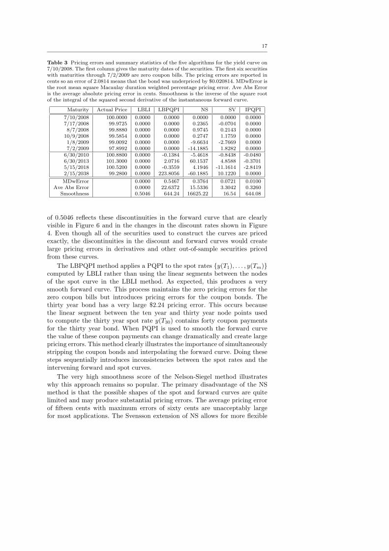
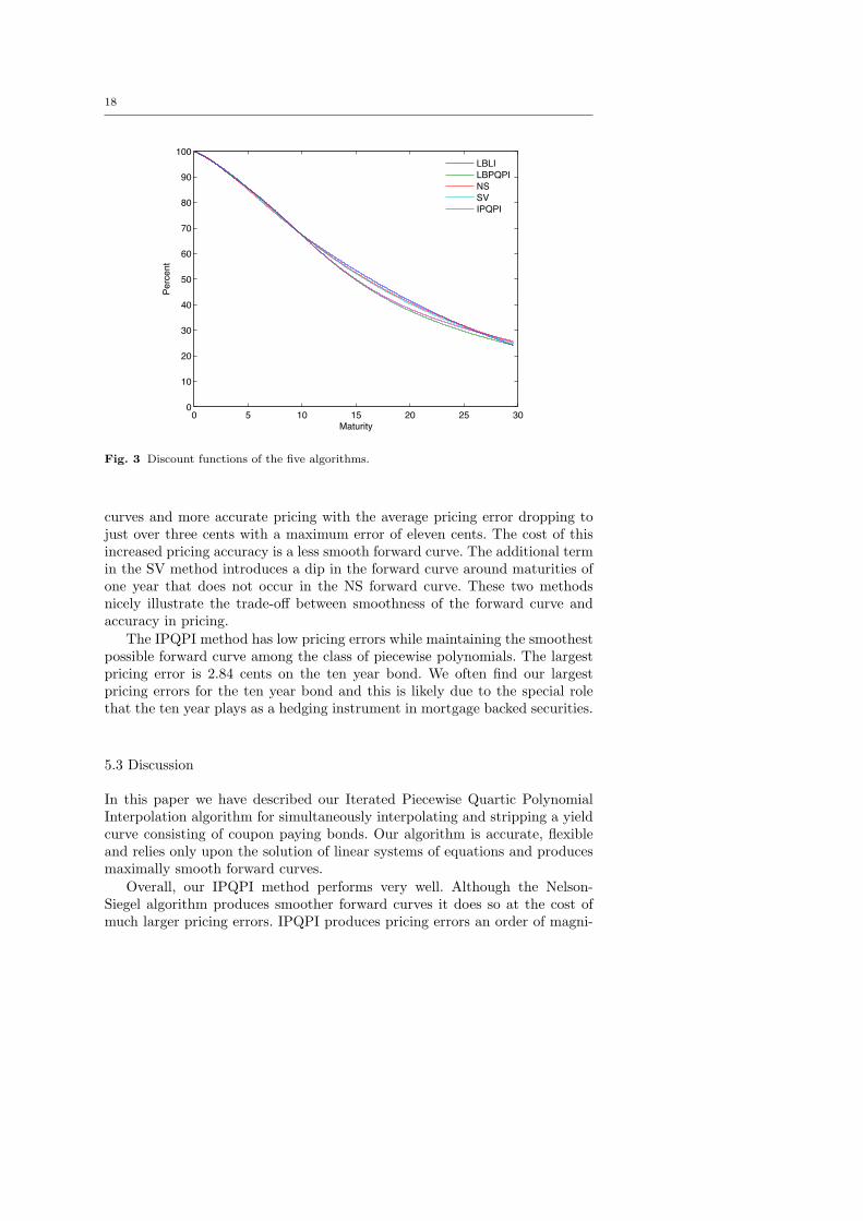
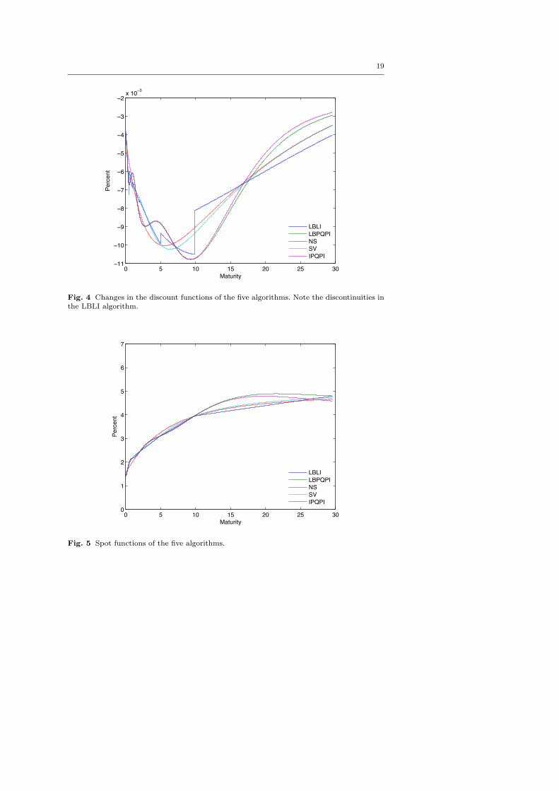
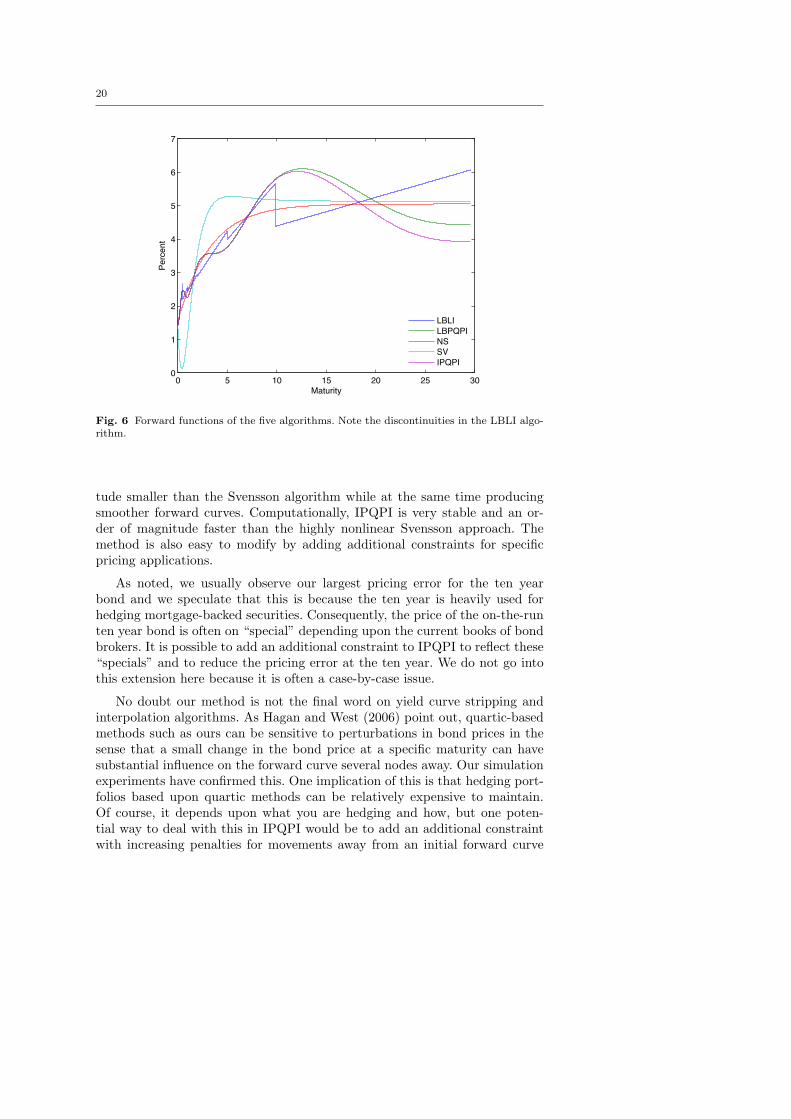
Figures 3 through 6 compare the discount functions, spot curves and in-stantaneous forward curves generated by each of these methods. Note that thediscount functions in Figure 3 and spot curves in Figure 5 for all the methodslook “reasonably” similar and it would be difficult to choose among them onthe basis of these curves alone. The changes in the discount function shownin Figure 4 and the forward curves shown in Figure 6, however, differ dra-matically. This is a visual indication of why modeling the forward rate curvedirectly is critical in fitting the yield curve.

Table 3 and the associated Figures 3 through 6 below illustrate the keyfeatures of the various methods and what we believe are the advantages of theIPQPI method. Note first that the LBLI method produces zero pricing errorsfor both the zero coupon bills and the coupon bearing bonds. This is preciselywhat the LBLI algorithm is designed to do. The spot yields at each nodeare chosen to exactly price the security maturing at that node. Since there isno feedback from one node to previous nodes during the computations, zeropricing errors is an easy criteria to satisfy. The problem with this method isthat, because the spot curve is piecewise linear, it produces discontinuities inthe spot and forward curves at the nodes. The reason for the discontinuitiesis clear from equations (11a) and (11b). The very low smoothness statistic

17

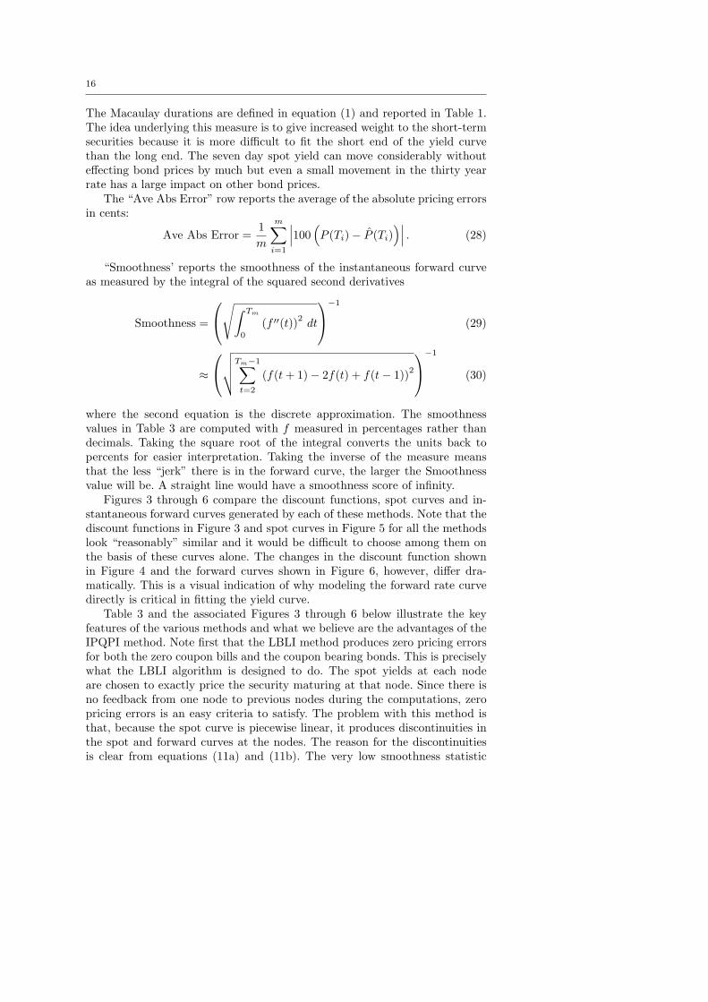
Table 3 Pricing errors and summary statistics of the five algorithms for the yield curve on7/10/2008. The first column gives the maturity dates of the securities. The first six securitieswith maturities through 7/2/2009 are zero coupon bills. The pricing errors are reported incents so an error of 2.0814 means that the bond was underpriced by $0.020814. MDwError isthe root mean square Macaulay duration weighted percentage pricing error. Ave Abs Erroris the average absolute pricing error in cents. Smoothness is the inverse of the square rootof the integral of the squared second derivative of the instantaneous forward curve.

Maturity Actual Price LBLI LBPQPI NS SV IPQPI

7/10/2008 100.0000 0.0000 0.0000 0.0000 0.0000 0.00007/17/2008 99.9725 0.0000 0.0000 0.2365 -0.0704 0.00008/7/2008 99.8880 0.0000 0.0000 0.9745 0.2143 0.0000

10/9/2008 99.5854 0.0000 0.0000 0.2747 1.1759 0.00001/8/2009 99.0092 0.0000 0.0000 -9.6634 -2.7669 0.00007/2/2009 97.8992 0.0000 0.0000 -14.1885 1.8282 0.0000

6/30/2010 100.8800 0.0000 -0.1384 -5.4618 -0.8438 -0.04806/30/2013 101.3000 0.0000 2.0716 60.1537 4.8588 -0.37015/15/2018 100.5200 0.0000 -0.3559 4.1946 -11.1614 -2.84192/15/2038 99.2800 0.0000 223.8056 -60.1885 10.1220 0.0000

MDwError 0.0000 0.5467 0.3764 0.0721 0.0100Ave Abs Error 0.0000 22.6372 15.5336 3.3042 0.3260

Smoothness 0.5046 644.24 16625.22 16.54 644.08

of 0.5046 reflects these discontinuities in the forward curve that are clearlyvisible in Figure 6 and in the changes in the discount rates shown in Figure4. Even though all of the securities used to construct the curves are pricedexactly, the discontinuities in the discount and forward curves would createlarge pricing errors in derivatives and other out-of-sample securities pricedfrom these curves.

The LBPQPI method applies a PQPI to the spot rates {y(T1), . . . , y(Tm)}computed by LBLI rather than using the linear segments between the nodesof the spot curve in the LBLI method. As expected, this produces a verysmooth forward curve. This process maintains the zero pricing errors for thezero coupon bills but introduces pricing errors for the coupon bonds. Thethirty year bond has a very large $2.24 pricing error. This occurs becausethe linear segment between the ten year and thirty year node points usedto compute the thirty year spot rate y(T30) contains forty coupon paymentsfor the thirty year bond. When PQPI is used to smooth the forward curvethe value of these coupon payments can change dramatically and create largepricing errors. This method clearly illustrates the importance of simultaneouslystripping the coupon bonds and interpolating the forward curve. Doing thesesteps sequentially introduces inconsistencies between the spot rates and theintervening forward and spot curves.

The very high smoothness score of the Nelson-Siegel method illustrateswhy this approach remains so popular. The primary disadvantage of the NSmethod is that the possible shapes of the spot and forward curves are quitelimited and may produce substantial pricing errors. The average pricing errorof fifteen cents with maximum errors of sixty cents are unacceptably largefor most applications. The Svensson extension of NS allows for more flexible

18

0 5 10 15 20 25 300

10

20

30

40

50

60

70

80

90

100

Maturity

Perc

ent

LBLILBPQPINSSVIPQPI

Fig. 3 Discount functions of the five algorithms.

curves and more accurate pricing with the average pricing error dropping tojust over three cents with a maximum error of eleven cents. The cost of thisincreased pricing accuracy is a less smooth forward curve. The additional termin the SV method introduces a dip in the forward curve around maturities ofone year that does not occur in the NS forward curve. These two methodsnicely illustrate the trade-off between smoothness of the forward curve andaccuracy in pricing.

The IPQPI method has low pricing errors while maintaining the smoothestpossible forward curve among the class of piecewise polynomials. The largestpricing error is 2.84 cents on the ten year bond. We often find our largestpricing errors for the ten year bond and this is likely due to the special rolethat the ten year plays as a hedging instrument in mortgage backed securities.

5.3 Discussion

In this paper we have described our Iterated Piecewise Quartic PolynomialInterpolation algorithm for simultaneously interpolating and stripping a yieldcurve consisting of coupon paying bonds. Our algorithm is accurate, flexibleand relies only upon the solution of linear systems of equations and producesmaximally smooth forward curves.

Overall, our IPQPI method performs very well. Although the Nelson-Siegel algorithm produces smoother forward curves it does so at the cost ofmuch larger pricing errors. IPQPI produces pricing errors an order of magni-

19

0 5 10 15 20 25 30−11

−10

−9

−8

−7

−6

−5

−4

−3

−2x 10−3

Maturity

Perc

ent

LBLILBPQPINSSVIPQPI

Fig. 4 Changes in the discount functions of the five algorithms. Note the discontinuities inthe LBLI algorithm.

0 5 10 15 20 25 300

1

2

3

4

5

6

7

Maturity

Perc

ent

LBLILBPQPINSSVIPQPI

Fig. 5 Spot functions of the five algorithms.

20

0 5 10 15 20 25 300

1

2

3

4

5

6

7

Maturity

Perc

ent

LBLILBPQPINSSVIPQPI

Fig. 6 Forward functions of the five algorithms. Note the discontinuities in the LBLI algo-rithm.

tude smaller than the Svensson algorithm while at the same time producingsmoother forward curves. Computationally, IPQPI is very stable and an or-der of magnitude faster than the highly nonlinear Svensson approach. Themethod is also easy to modify by adding additional constraints for specificpricing applications.

As noted, we usually observe our largest pricing error for the ten yearbond and we speculate that this is because the ten year is heavily used forhedging mortgage-backed securities. Consequently, the price of the on-the-runten year bond is often on “special” depending upon the current books of bondbrokers. It is possible to add an additional constraint to IPQPI to reflect these“specials” and to reduce the pricing error at the ten year. We do not go intothis extension here because it is often a case-by-case issue.

No doubt our method is not the final word on yield curve stripping andinterpolation algorithms. As Hagan and West (2006) point out, quartic-basedmethods such as ours can be sensitive to perturbations in bond prices in thesense that a small change in the bond price at a specific maturity can havesubstantial influence on the forward curve several nodes away. Our simulationexperiments have confirmed this. One implication of this is that hedging port-folios based upon quartic methods can be relatively expensive to maintain.Of course, it depends upon what you are hedging and how, but one poten-tial way to deal with this in IPQPI would be to add an additional constraintwith increasing penalties for movements away from an initial forward curve

21

at a specific maturity. Our method is flexible enough to easily add such con-straints.

Another issue worth exploring is the dependency of IPQPI on polynomials.One of the reasons that the Nelson and Siegel and the Svensson methods workso well is that they use exponential functions that are essentially infinite orderpolynomials with highly constrained coefficients. It is likely that a more generalclass of basis functions would produce better results albeit at a much highercomputational cost.

A Appendix: Piecewise Quartic Polynomial Interpolation (PQPI)

The procedure for interpolating the zero coupon portion of the yield curve is similar tothat described in Lim and Xiao (2002) except that we handle the terminal condition onthe forward curve differently. Our approach adds one additional segment to the piecewisespline function with some additional coefficient restrictions on the terminal spline. Since thematrix sizes differ to reflect these changes, we provide the details of this step here.

In the first subsection of the appendix we show how to construct the objective functionas a quadratic expression. In the second subsection we construct the constraints as linearequations and in the final subsection we show how to solve the PQPI system.

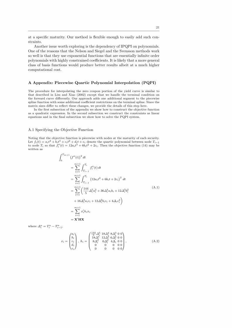
A.1 Specifying the Objective Function

Noting that the objective function is piecewise with nodes at the maturity of each security.Let fi(t) = ait

4 + bit3 + cit

2 + dit + ei denote the quartic polynomial between node Ti−1

to node Ti so that f ′′i (t) = 12ait3 + 6bit

2 + 2ci. Then the objective function (14) may bewritten as Z Tm+1

0

`f ′′(t)

´2dt

=

m+1Xi=1

Z Ti

Ti−1

f ′′i (t) dt

=

m+1Xi=1

Z Ti

Ti−1

`12ait

2 + 6bit+ 2ci´2dt

=

m+1Xi=1

„144

5∆5

i a2i + 36∆4

i aibi + 12∆3i b

2i

+ 16∆3i aici + 12∆2

i bici + 4∆ic2i

«

=

m+1Xi=1

x′ihixi

= X′HX

(A.1)

where ∆ni = Tn

i − Tni−1,

xi =

0BBB@ai

bicidi

ei

1CCCA , hi =

0BBBB@1445∆5

i 18∆4i 8∆3

i 0 018∆4

i 12∆3i 6∆2

i 0 08∆3

i 6∆2i 4∆i 0 0

0 0 0 0 00 0 0 0 0

1CCCCA , (A.2)

22

X =

0B@ x1

...xm+1

1CA5(m+1)×1

, (A.3)

H =

0BBB@h1 0 0 · · · 00 h2 0 · · · 0...

. . ....

0 0 0 · · · hm+1

1CCCA5(m+1)×5(m+1)

, (A.4)

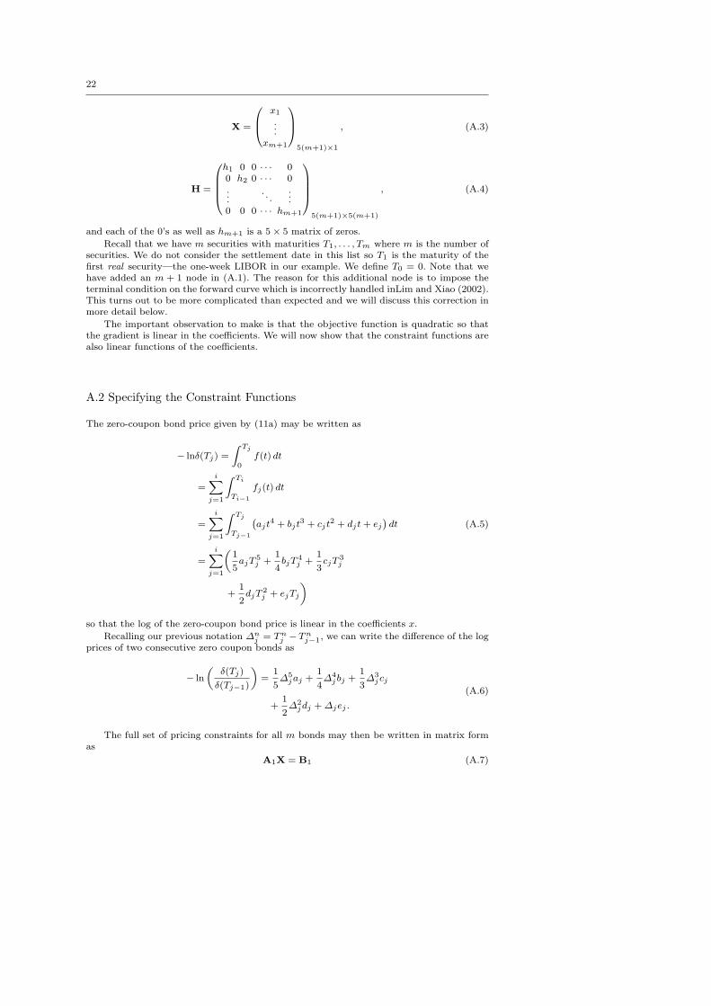
and each of the 0’s as well as hm+1 is a 5× 5 matrix of zeros.

Recall that we have m securities with maturities T1, . . . , Tm where m is the number ofsecurities. We do not consider the settlement date in this list so T1 is the maturity of thefirst real security—the one-week LIBOR in our example. We define T0 = 0. Note that wehave added an m + 1 node in (A.1). The reason for this additional node is to impose theterminal condition on the forward curve which is incorrectly handled inLim and Xiao (2002).This turns out to be more complicated than expected and we will discuss this correction inmore detail below.

The important observation to make is that the objective function is quadratic so thatthe gradient is linear in the coefficients. We will now show that the constraint functions arealso linear functions of the coefficients.

A.2 Specifying the Constraint Functions

The zero-coupon bond price given by (11a) may be written as

− lnδ(Tj) =

Z Tj

0f(t) dt

=iX

j=1

Z Ti

Ti−1

fj(t) dt

=

iXj=1

Z Tj

Tj−1

`ajt

4 + bjt3 + cjt

2 + djt+ ej

´dt

=

iXj=1

„1

5ajT

5j +

1

4bjT

4j +

1

3cjT

3j

+1

2djT

2j + ejTj

«

(A.5)

so that the log of the zero-coupon bond price is linear in the coefficients x.

Recalling our previous notation ∆nj = Tn

j − Tnj−1, we can write the difference of the log

prices of two consecutive zero coupon bonds as

− ln

„δ(Tj)

δ(Tj−1)

«=

1

5∆5

jaj +1

4∆4

j bj +1

3∆3

jcj

+1

2∆2

jdj +∆jej .

(A.6)

The full set of pricing constraints for all m bonds may then be written in matrix formas

A1X = B1 (A.7)

23

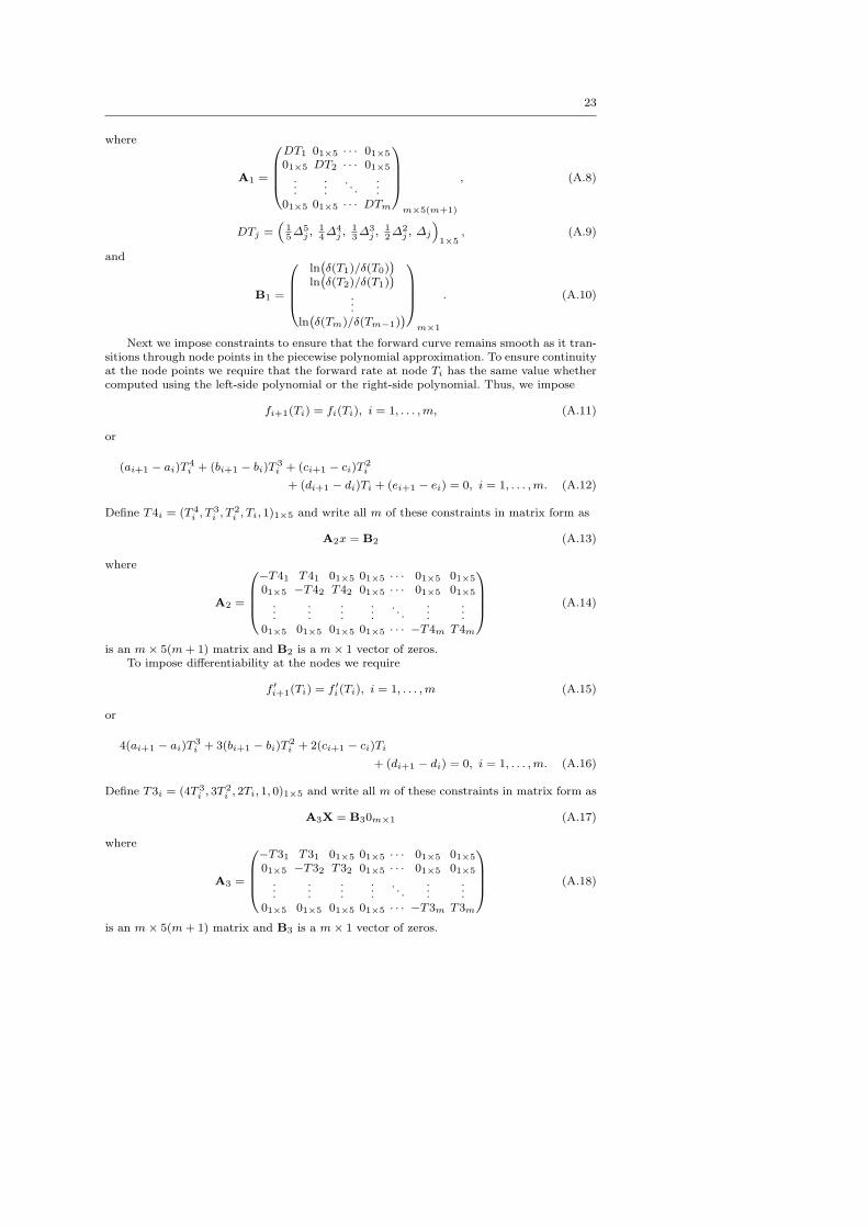
where

A1 =

0BBB@DT1 01×5 · · · 01×5

01×5 DT2 · · · 01×5

......

. . ....

01×5 01×5 · · · DTm

1CCCAm×5(m+1)

, (A.8)

DTj =“

15∆5

j ,14∆4

j ,13∆3

j ,12∆2

j , ∆j

”1×5

, (A.9)

and

B1 =

0BBB@ln`δ(T1)/δ(T0)

´ln`δ(T2)/δ(T1)

´...

ln`δ(Tm)/δ(Tm−1)

´1CCCA

m×1

. (A.10)

Next we impose constraints to ensure that the forward curve remains smooth as it tran-sitions through node points in the piecewise polynomial approximation. To ensure continuityat the node points we require that the forward rate at node Ti has the same value whethercomputed using the left-side polynomial or the right-side polynomial. Thus, we impose

fi+1(Ti) = fi(Ti), i = 1, . . . ,m, (A.11)

or

(ai+1 − ai)T4i + (bi+1 − bi)T 3

i + (ci+1 − ci)T 2i

+ (di+1 − di)Ti + (ei+1 − ei) = 0, i = 1, . . . ,m. (A.12)

Define T4i = (T 4i , T

3i , T

2i , Ti, 1)1×5 and write all m of these constraints in matrix form as

A2x = B2 (A.13)

where

A2 =

0BBB@−T41 T41 01×5 01×5 · · · 01×5 01×5

01×5 −T42 T42 01×5 · · · 01×5 01×5

......

......

. . ....

...01×5 01×5 01×5 01×5 · · · −T4m T4m

1CCCA (A.14)

is an m× 5(m+ 1) matrix and B2 is a m× 1 vector of zeros.To impose differentiability at the nodes we require

f ′i+1(Ti) = f ′i(Ti), i = 1, . . . ,m (A.15)

or

4(ai+1 − ai)T3i + 3(bi+1 − bi)T 2

i + 2(ci+1 − ci)Ti

+ (di+1 − di) = 0, i = 1, . . . ,m. (A.16)

Define T3i = (4T 3i , 3T

2i , 2Ti, 1, 0)1×5 and write all m of these constraints in matrix form as

A3X = B30m×1 (A.17)

where

A3 =

0BBB@−T31 T31 01×5 01×5 · · · 01×5 01×5

01×5 −T32 T32 01×5 · · · 01×5 01×5

......

......

. . ....

...01×5 01×5 01×5 01×5 · · · −T3m T3m

1CCCA (A.18)

is an m× 5(m+ 1) matrix and B3 is a m× 1 vector of zeros.

24

To ensure that the first derivatives of the forward curve are smooth at the nodes weimpose

f ′′i+1(Ti) = f ′′i (Ti), i = 1, . . . ,m, (A.19)

or

12(ai+1 − ai)T2i + 6(bi+1 − bi)Ti

+ 2(ci+1 − ci) = 0, i = 1, . . . ,m. (A.20)

Define T2i = (12T 2i , 6Ti, 2, 1, 0, 0)1×5 and write all m of these constraints in matrix form as

A4X = B4 (A.21)

where

A4 =

0BBB@−T21 T21 01×5 01×5 · · · 01×5 01×5

01×5 −T22 T22 01×5 · · · 01×5 01×5

......

......

. . ....

...01×5 01×5 01×5 01×5 · · · −T2m T2m

1CCCA (A.22)

is an m× 5(m+ 1) matrix and B4 is a m× 1 vector of zeros.

To ensure the boundary condition f(0) = y0, we simply impose e1 = y0. The terminalboundary condition f ′(Tm) = 0 is more difficult to impose. Lim and Xiao (2002) use thecondition d1 = 0 which is clearly incorrect. We impose the terminal condition by adding anadditional (m + 1)st segment to the piecewise polynomial with the coefficient restrictionsam+1 = bm+1 = cm+1 = dm+1 = 0 so that f(t) = em+1 for all t > Tm. The terminal heightof the forward function is left unconstrained and the continuity and smoothness constraintsdescribed above will ensure a smooth transition to the zero slope of the forward curve atnode Tm.

These five boundary conditions may be written in matrix notation as

A5X = B5 (A.23)

where

A5 =

0BBB@0 0 0 0 1 0 · · · 0 0 0 0 00 0 0 0 0 0 · · · 1 0 0 0 00 0 0 0 0 0 · · · 0 1 0 0 00 0 0 0 0 0 · · · 0 0 1 0 00 0 0 0 0 0 · · · 0 0 0 1 0

1CCCA5×5(m+1)

(A.24)

and

B5 =

0BBB@y00000

1CCCA . (A.25)

Stacking all of these linear constraints gives

AX = B (A.26)

where

A =

0BBB@A1

A2

A3

A4

A5

1CCCA(4m+5)×5(m+1)

and

0BBB@B1

B2

B3

B4

B5

1CCCA(4m+5)×1

. (A.27)

25

A.3 Solving the PQPI System

The constrained optimization problem may now be written in matrix notation as

minX,λ

Z(X,λ) = X′HX + λ′(AX−B) (A.28)

where λ is the 4m+ 5 vector of Lagrange multipliers corresponding to the constraints.The first-order conditions are

∂

∂XZ(X,λ) = 2HX + A′λ = 0 (A.29)

and∂

∂λZ(X,λ) = AHX−B = 0, (A.30)

or „2H A′

A 0

«„Xλ

«=

„0B

«(A.31)

from which we find the explicit solution„X∗

λ∗

«=

„2H A′

A 0

«−1 „0B

«. (A.32)

References

Adams, K. (2001). Smooth interpolation of zero curves. ALGO Research Quarterly,4(1/2):11–22.

Adams, K. and van Deventer, D. (1994). Fitting yield curves and forward rate curves withmaximum smoothness. The Journal of Fixed Income, 4(1):52–62.

Diebold, F. X. and Li, C. (2006). Forecasting the term structure of government bond yields.Journal of Econometrics, 130:337–364.

Fisher, M. (2004). Modeling the term structure of interest rates: An introduction. FederalReserve Bank of Atlanta Economic Review, 89(3):41–62.

Gimeno, R. and Nave, J. M. (2006). Genetic algorithm estimation of interest rate termstructure. Technical Report 0634, Banco de Espana.

Hagan, P. S. and West, G. (2006). Interpolation methods for curve construction. AppliedMathematical Finance, 13 (2):89–129.

Jordan, J. V. and Mansi, S. A. (2003). Term structure estimation from on-the-run treasuries.Journal of Banking & Finance, 27.

Lim, K. G. and Xiao, Q. (2002). Computing maximum smoothness forward rate curves.Journanl of Statistics and Computing, 12(3):275–279.

Manzano, J. and Blomvall, J. (2004). Positive forward rates in the maximum smoothnessframework. Quantitative Finance, 4(2):221–232.

McCulloch, J. H. (1971). Measuring the term structure of interest rates. The Journal ofBusiness, 44 (1):19–31.

McCulloch, J. H. (1975). The tax-adjusted yield curve. The Journal of Finance, 30 (3):811–830.

Nelson, C. R. and Siegel, A. F. (1987). Parsimonious modeling of yield curves. The Journalof Business, 60 (4):473–489.

Svensson, L. E. O. (1995). Estimating forward interest rates with the extended nelson &siegel method. Sveriges Riksbank Quarterly Review, 3:13–26.

Vasicek, O. A. and Fong, H. G. (1982). Term structure modeling using exponential splines.The Journal of Finance, 37 (2):339–348.