COMPUTERS & STRUCTURES INC. Software Verificationextras.springer.com/2003/978-3-322-80050-3/INFORMATION and POOL/SAP200… · COMPUTERS & STRUCTURES INC. R Software Verification PROGRAM

C OMP UTE R S &S TRU CTU R ES

IN C.

R Software VerificationPROGRAM NAME: SAP2000REVISION NO.: 0

EXAMPLE 6-006 - 1

EXAMPLE 6-006LINK – SUNY BUFFALO DAMPER WITH LINEAR VELOCITY EXPONENT

PROBLEM DESCRIPTION

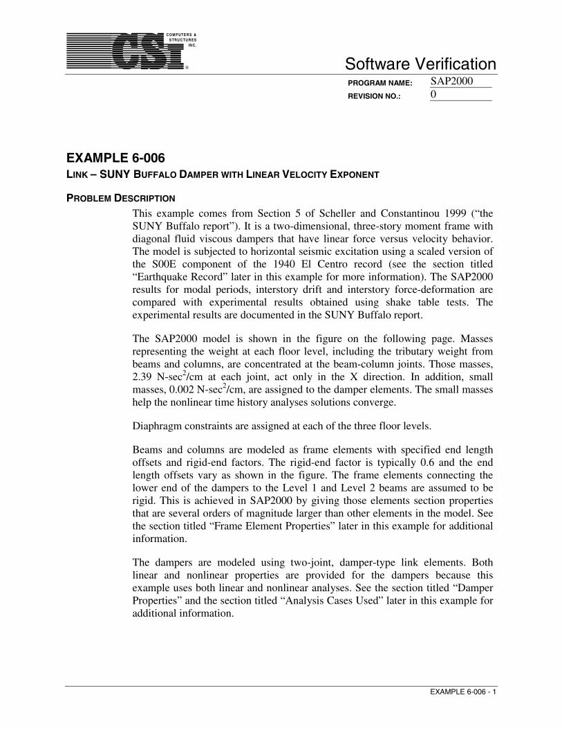
This example comes from Section 5 of Scheller and Constantinou 1999 (“theSUNY Buffalo report”). It is a two-dimensional, three-story moment frame withdiagonal fluid viscous dampers that have linear force versus velocity behavior.The model is subjected to horizontal seismic excitation using a scaled version ofthe S00E component of the 1940 El Centro record (see the section titled“Earthquake Record” later in this example for more information). The SAP2000results for modal periods, interstory drift and interstory force-deformation arecompared with experimental results obtained using shake table tests. Theexperimental results are documented in the SUNY Buffalo report.

The SAP2000 model is shown in the figure on the following page. Massesrepresenting the weight at each floor level, including the tributary weight frombeams and columns, are concentrated at the beam-column joints. Those masses,2.39 N-sec2/cm at each joint, act only in the X direction. In addition, smallmasses, 0.002 N-sec2/cm, are assigned to the damper elements. The small masseshelp the nonlinear time history analyses solutions converge.

Diaphragm constraints are assigned at each of the three floor levels.

Beams and columns are modeled as frame elements with specified end lengthoffsets and rigid-end factors. The rigid-end factor is typically 0.6 and the endlength offsets vary as shown in the figure. The frame elements connecting thelower end of the dampers to the Level 1 and Level 2 beams are assumed to berigid. This is achieved in SAP2000 by giving those elements section propertiesthat are several orders of magnitude larger than other elements in the model. Seethe section titled “Frame Element Properties” later in this example for additionalinformation.

The dampers are modeled using two-joint, damper-type link elements. Bothlinear and nonlinear properties are provided for the dampers because thisexample uses both linear and nonlinear analyses. See the section titled “DamperProperties” and the section titled “Analysis Cases Used” later in this example foradditional information.


IN C.


EXAMPLE 6-006 - 2

GEOMETRY AND PROPERTIES

Level 3

Level 2

Level 1

Base

1STC

OL

10 c

m10

cm

10 c

m

18.8

cm1

Stiff

15 c

m40.25 cm

40.25 cm

10 cm 10 cm

120.5 cm

26 c

m

100.

5 cm

76.2

cm

76.2

cm

3

5

7

2

4

6

8

98 cm

10

11

12

13

26 c

m

X

Y

Damper

Damper

Damper

Stiff

2XST2X3

2XST2X3

2XST2X3

ST2X

385

ST2X

385

1STC

OL

ST2X

385

ST2X

385 10

cm

Joints constrained as diaphragm, typical at Levels 1, 2, and 3

Frame element end length offsets, typical. Rigid-end factor is 0.6

2.39 N-sec2/cm mass at joints 3, 4, 5, 6, 7 and 8 acting in X direction only

20 c

m


IN C.


EXAMPLE 6-006 - 3

FRAME ELEMENT PROPERTIES

The frame elements in the SAP2000 model have the following materialproperties.

E = 21,000,000 N/cm2

ν = 0.3

The frame elements in the SAP2000 model have the following section properties.

1STCOLA = 9.01 cm2

I = 14.614 cm4

Av = 4.42 cm2

ST2X385A = 6.61 cm2

I = 5.95 cm4

Av = 2.02 cm2

2XST2X3A = 13.22 cm2

I = 11.9 cm4

Av = 2.02 cm2

STIFFA = 10,000 cm2

I = 100,000 cm4

Av = 0 cm2 (shear deformations not included)


IN C.


EXAMPLE 6-006 - 4

DAMPER PROPERTIES

The damper elements in the SAP2000 model have the following properties.

Linear (k is in parallel with c)k = 0 N/cmc = 160 N-sec/cm

Nonlinear (k is in series with c)k = 1,000,000 N/cmc = 160 N-sec/cmexp= 1

The damping coefficient used for the dampers for both the linear and nonlinearanalyses is c = 160 N-sec/cm. This value was determined using the average valuefrom a series of experimental tests. As described in Scheller and Constantinou1999, the tested values of the damping coefficient ranged from 135 to 185 N-sec/cm. The average value of 160 N-sec/cm was used for all dampers in theSAP2000 model

LINEAR AND NONLINEAR ANALYSIS USING DAMPERS

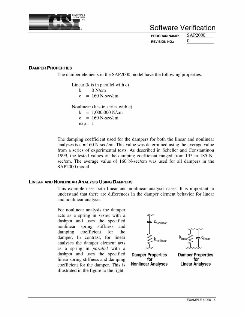
This example uses both linear and nonlinear analysis cases. It is important tounderstand that there are differences in the damper element behavior for linearand nonlinear analysis.

For nonlinear analysis the damperacts as a spring in series with adashpot and uses the specifiednonlinear spring stiffness anddamping coefficient for thedamper. In contrast, for linearanalyses the damper element actsas a spring in parallel with adashpot and uses the specifiedlinear spring stiffness and dampingcoefficient for the damper. This isillustrated in the figure to the right.

Damper Propertiesfor

Nonlinear Analyses

knonlinear

cnonlinear

clinearklinear

Damper Propertiesfor

Linear Analyses


IN C.


EXAMPLE 6-006 - 5

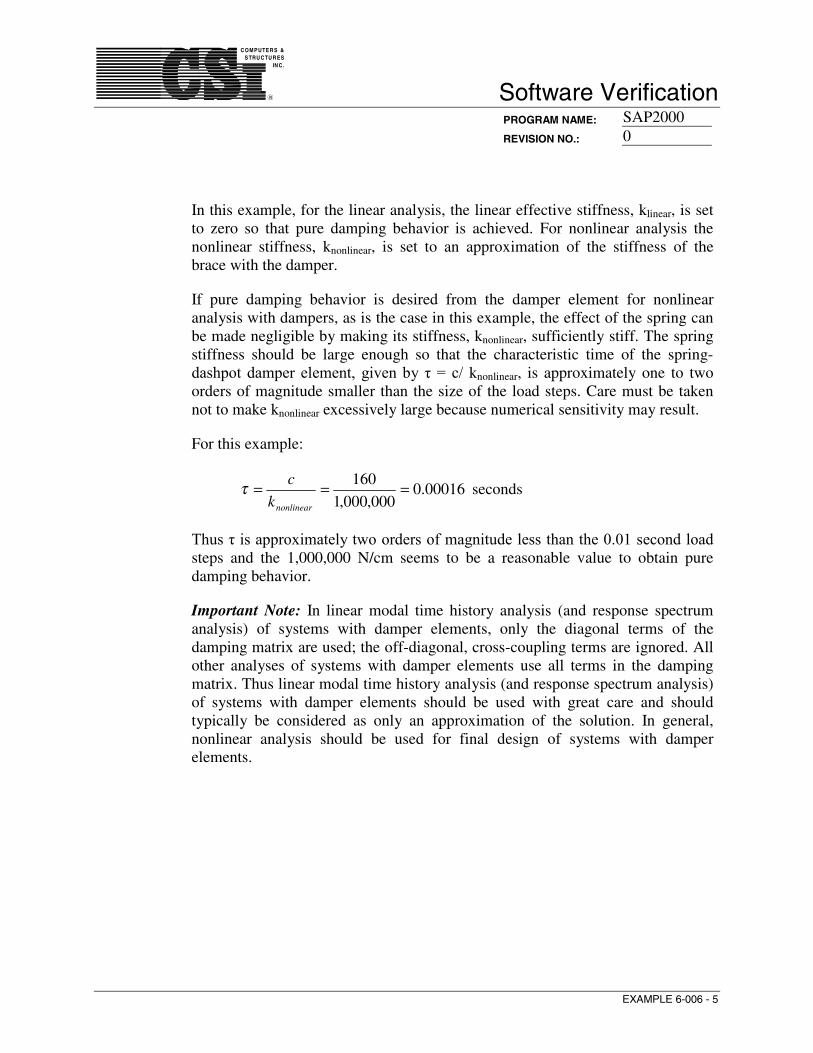
In this example, for the linear analysis, the linear effective stiffness, klinear, is setto zero so that pure damping behavior is achieved. For nonlinear analysis thenonlinear stiffness, knonlinear, is set to an approximation of the stiffness of thebrace with the damper.

If pure damping behavior is desired from the damper element for nonlinearanalysis with dampers, as is the case in this example, the effect of the spring canbe made negligible by making its stiffness, knonlinear, sufficiently stiff. The springstiffness should be large enough so that the characteristic time of the spring-dashpot damper element, given by τ = c/ knonlinear, is approximately one to twoorders of magnitude smaller than the size of the load steps. Care must be takennot to make knonlinear excessively large because numerical sensitivity may result.

For this example:

00016.0000,000,1

160 ===nonlineark

cτ seconds

Thus τ is approximately two orders of magnitude less than the 0.01 second loadsteps and the 1,000,000 N/cm seems to be a reasonable value to obtain puredamping behavior.

Important Note: In linear modal time history analysis (and response spectrumanalysis) of systems with damper elements, only the diagonal terms of thedamping matrix are used; the off-diagonal, cross-coupling terms are ignored. Allother analyses of systems with damper elements use all terms in the dampingmatrix. Thus linear modal time history analysis (and response spectrum analysis)of systems with damper elements should be used with great care and shouldtypically be considered as only an approximation of the solution. In general,nonlinear analysis should be used for final design of systems with damperelements.


IN C.


EXAMPLE 6-006 - 6

ANALYSIS CASES USED

Five different analysis cases are run for this example. They are described in thefollowing table.

Analysis Case Description

MODAL Modal analysis case for ritz vectors. Ninety-nine modes arerequested. The program will automatically determine that amaximum of ten modes are possible and thus reduce thenumber of modes to ten. The starting vectors are Ux

acceleration and all link element nonlinear degrees offreedom.

MHIST1 Linear modal time history analysis case that uses the modesin the MODAL analysis case. This case includes modaldamping in modes 1, 2 and 3.

NLMHIST1 Nonlinear modal time history analysis case that uses themodes in the MODAL analysis case. This case includesmodal damping in modes 1, 2 and 3.

DHIST1 Linear direct integration time history analysis case. Thiscase includes proportional damping.

NLDHIST1 Nonlinear direct integration time history analysis case. Thiscase includes proportional damping.

The modal time history analyses use 2.71%, 1.02% and 1.04% modal dampingfor modes 1, 2 and 3, respectively. As described in Scheller and Constantinou1999, those modal damping values were determined by experiment for the framewithout dampers.


IN C.


EXAMPLE 6-006 - 7

The direct integration timehistories use mass andstiffness proportional dampingthat is specified to have 2.71%damping at a the period of thefirst mode and 1.02%damping at the period of thesecond mode. The solid line inthe figure to the right showsthe proportional damping usedin this example.

EARTHQUAKE RECORD

The following figure shows the earthquake record used in this example. Asdescribed in Scheller and Constantinou 1999, it is the S00E component of the1940 El Centro record compressed in time by a factor of two. It is compressed tosatisfy the similitude requirements of the quarter length scale model used in theshake table tests.

The earthquake record is provided in a file named EQ6-006.txt. This file has oneacceleration value per line, in g. The acceleration values are provided at an equalspacing of 0.01 second.

-0.4

-0.3

-0.2

-0.1

0

0.1

0.2

0.3

0 5 10 15 20 25 30 35 40

Time (sec)

Acc

eler

atio

n (

cm/s

ec2 )

0

0.01

0.02

0.03

0.04

0.05

0 0.05 0.1 0.15 0.2 0.25 0.3 0.35 0.4 0.45 0.5

Period (sec)D

amp

ing

Rat

io

Mass Stiffness Rayleigh


IN C.


EXAMPLE 6-006 - 8

TECHNICAL FEATURES OF SAP2000 TESTED

Damper links with linear velocity exponents Frame end length offsets Joint mass assignments Modal analysis for ritz vectors Linear modal time history analysis Nonlinear modal time history analysis Linear direct integration time history analysis Nonlinear direct integration time history analysis Generalized displacements

RESULTS COMPARISON

Independent results are experimental results from shake table testing presented inSection 5, pages 61 through 73, of Scheller and Constantinou 1999.

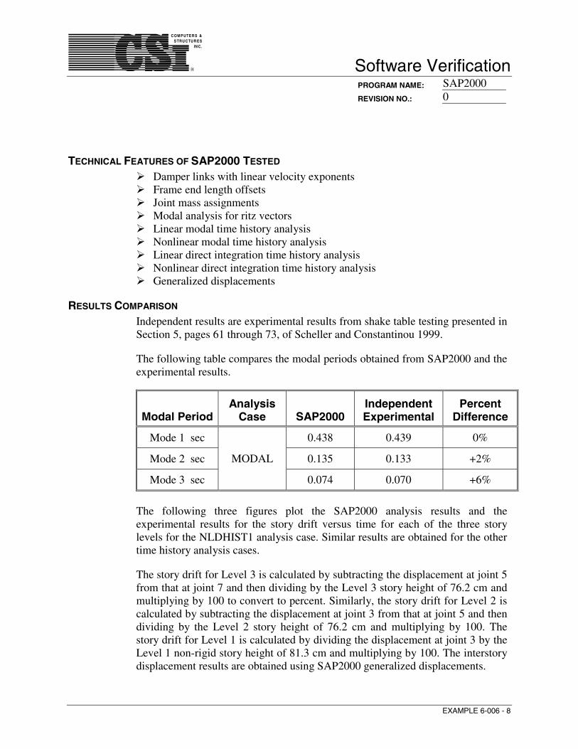
The following table compares the modal periods obtained from SAP2000 and theexperimental results.

Modal PeriodAnalysis

Case SAP2000IndependentExperimental

PercentDifference

Mode 1 sec 0.438 0.439 0%

Mode 2 sec 0.135 0.133 +2%

Mode 3 sec

MODAL

0.074 0.070 +6%

The following three figures plot the SAP2000 analysis results and theexperimental results for the story drift versus time for each of the three storylevels for the NLDHIST1 analysis case. Similar results are obtained for the othertime history analysis cases.

The story drift for Level 3 is calculated by subtracting the displacement at joint 5from that at joint 7 and then dividing by the Level 3 story height of 76.2 cm andmultiplying by 100 to convert to percent. Similarly, the story drift for Level 2 iscalculated by subtracting the displacement at joint 3 from that at joint 5 and thendividing by the Level 2 story height of 76.2 cm and multiplying by 100. Thestory drift for Level 1 is calculated by dividing the displacement at joint 3 by theLevel 1 non-rigid story height of 81.3 cm and multiplying by 100. The interstorydisplacement results are obtained using SAP2000 generalized displacements.


IN C.


EXAMPLE 6-006 - 9

-1

-0.8

-0.6

-0.4

-0.2

0

0.2

0.4

0.6

0.8

1

0 2 4 6 8 10 12 14 16 18 20

Time (sec)

Lev

el 3

Sto

ry D

rift

(%

)

NLDHIST1

Experimental

-1

-0.8

-0.6

-0.4

-0.2

0

0.2

0.4

0.6

0.8

1

0 2 4 6 8 10 12 14 16 18 20

Time (sec)

Lev

el 2

Sto

ry D

rift

(%

)

NLDHIST1

Experimental

-1

-0.8

-0.6

-0.4

-0.2

0

0.2

0.4

0.6

0.8

1

0 2 4 6 8 10 12 14 16 18 20

Time (sec)

Lev

el 1

Sto

ry D

rift

(%

)

NLDHIST1

Experimental


IN C.


EXAMPLE 6-006 - 10

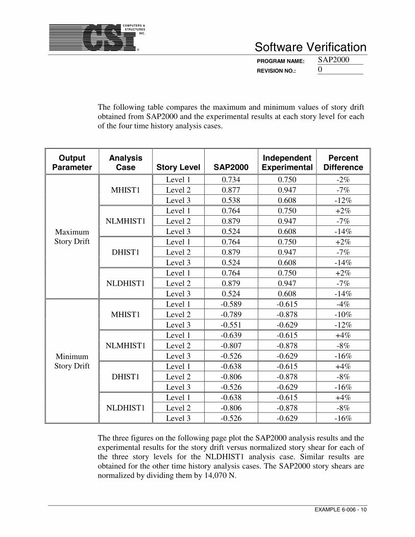
The following table compares the maximum and minimum values of story driftobtained from SAP2000 and the experimental results at each story level for eachof the four time history analysis cases.

OutputParameter

AnalysisCase Story Level SAP2000

IndependentExperimental

PercentDifference

Level 1 0.734 0.750 -2%Level 2 0.877 0.947 -7%MHIST1Level 3 0.538 0.608 -12%Level 1 0.764 0.750 +2%Level 2 0.879 0.947 -7%NLMHIST1Level 3 0.524 0.608 -14%Level 1 0.764 0.750 +2%Level 2 0.879 0.947 -7%DHIST1Level 3 0.524 0.608 -14%Level 1 0.764 0.750 +2%Level 2 0.879 0.947 -7%

MaximumStory Drift

NLDHIST1Level 3 0.524 0.608 -14%Level 1 -0.589 -0.615 -4%Level 2 -0.789 -0.878 -10%MHIST1Level 3 -0.551 -0.629 -12%Level 1 -0.639 -0.615 +4%Level 2 -0.807 -0.878 -8%NLMHIST1Level 3 -0.526 -0.629 -16%Level 1 -0.638 -0.615 +4%Level 2 -0.806 -0.878 -8%DHIST1Level 3 -0.526 -0.629 -16%Level 1 -0.638 -0.615 +4%Level 2 -0.806 -0.878 -8%

MinimumStory Drift

NLDHIST1Level 3 -0.526 -0.629 -16%

The three figures on the following page plot the SAP2000 analysis results and theexperimental results for the story drift versus normalized story shear for each ofthe three story levels for the NLDHIST1 analysis case. Similar results areobtained for the other time history analysis cases. The SAP2000 story shears arenormalized by dividing them by 14,070 N.


IN C.


EXAMPLE 6-006 - 11

-0.4

-0.3

-0.2

-0.1

0

0.1

0.2

0.3

0.4

-1 -0.8 -0.6 -0.4 -0.2 0 0.2 0.4 0.6 0.8 1

Level 3 Story Drift (%)

Lev

el 3

Sto

ry S

hea

r / W

eig

ht

Experimental

NLDHIST1

Story Height for Drift = 76.2 cm

Structure Weight for Shear Normalization = 14,070 N

-0.4

-0.3

-0.2

-0.1

0

0.1

0.2

0.3

0.4

-1 -0.8 -0.6 -0.4 -0.2 0 0.2 0.4 0.6 0.8 1


Lev

el 2

Sto

ry S

hea

r / W

eig

ht

Experimental

NLDHIST1



-0.4

-0.3

-0.2

-0.1

0

0.1

0.2

0.3

0.4

-1 -0.8 -0.6 -0.4 -0.2 0 0.2 0.4 0.6 0.8 1


Lev

el 1

Sto

ry S

hea

r / W

eig

ht

Experimental

NLDHIST1




IN C.


EXAMPLE 6-006 - 12

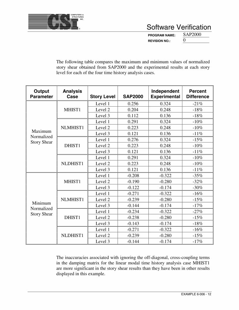
The following table compares the maximum and minimum values of normalizedstory shear obtained from SAP2000 and the experimental results at each storylevel for each of the four time history analysis cases.

OutputParameter

AnalysisCase Story Level SAP2000

IndependentExperimental

PercentDifference

Level 1 0.256 0.324 -21%Level 2 0.204 0.248 -18%MHIST1Level 3 0.112 0.136 -18%Level 1 0.291 0.324 -10%Level 2 0.223 0.248 -10%NLMHIST1Level 3 0.121 0.136 -11%Level 1 0.276 0.324 -15%Level 2 0.223 0.248 -10%DHIST1Level 3 0.121 0.136 -11%Level 1 0.291 0.324 -10%Level 2 0.223 0.248 -10%

MaximumNormalizedStory Shear

NLDHIST1Level 3 0.121 0.136 -11%Level 1 -0.208 -0.322 -35%Level 2 -0.190 -0.280 -32%MHIST1Level 3 -0.122 -0.174 -30%Level 1 -0.271 -0.322 -16%Level 2 -0.239 -0.280 -15%NLMHIST1Level 3 -0.144 -0.174 -17%Level 1 -0.234 -0.322 -27%Level 2 -0.238 -0.280 -15%DHIST1Level 3 -0.143 -0.174 -18%Level 1 -0.271 -0.322 -16%Level 2 -0.239 -0.280 -15%

MinimumNormalizedStory Shear

NLDHIST1Level 3 -0.144 -0.174 -17%

The inaccuracies associated with ignoring the off-diagonal, cross-coupling termsin the damping matrix for the linear modal time history analysis case MHIST1are more significant in the story shear results than they have been in other resultsdisplayed in this example.


IN C.


EXAMPLE 6-006 - 13

The Level 1 story shear results shown for the MHIST1 analysis case do notinclude the force in the Level 1 damper. This damper force is not reportedbecause, for the linear modal time history, the damping associated with thedampers is converted to modal damping and added to any other modal dampingthat may be specified. If a stiff frame element was included in the model belowthe Level 1 damper, similar to the stiff element at the other levels, the Level 1story shear could be cut through three frame elements and all of the shear wouldbe accounted for. However, the inaccuracies caused by ignoring the off-diagonalterms in the damping matrix would still be present.

COMPUTER FILE: Example 6-006

CONCLUSION

The SAP2000 results show an acceptable comparison with the independentresults. The clearest comparison of results is evident in the graphicalcomparisons.

The results using linear modal time history analysis (analysis case MHIST1) areslightly different from the other analyses because the linear modal time historyanalysis uses only the diagonal terms in the damping matrix, ignoring any off-diagonal, cross-coupling terms. The other analyses use all terms in the dampingmatrix. For this example analysis case MHIST1 shows a good approximation ofthe other solutions. The error introduced by ignoring the cross-coupling termstends to improve the comparison with experimental results in some items and tomake it worse in other items.

In general we recommend that linear modal time history analysis of models withdamper elements only be used for quick, preliminary checks, and that anothertype of analysis be used for final analysis.

Documents

COMPUTERS & STRUCTURES INC. Software Verificationextras.springer.com/2003/978-3-322-80050-3/INFORMATION and POOL/SAP200… · COMPUTERS & STRUCTURES INC. R Software Verification PROGRAM