Embed Size (px)
Citation preview

Computers and Fluids 153 (2017) 1–19
Contents lists available at ScienceDirect
Computers and Fluids
journal homepage: www.elsevier.com/locate/compfluid
Implementation of the Ghost Fluid Method for free surface flows in
polyhedral Finite Volume framework
Vuko Vuk ̌cevi ́c
a , ∗, Hrvoje Jasak
a , b , Inno Gatin
a
a University of Zagreb, Faculty of Mechanical Engineering and Naval Architecture, Ivana Lu ̌ci ́ca 5, Zagreb, Croatia b Wikki Ltd, 459 Southbank House, SE1 7SJ London, United Kingdom
a r t i c l e i n f o
Article history:
Received 25 August 2016
Revised 13 April 2017
Accepted 3 May 2017
Available online 4 May 2017
Keywords:
Ghost Fluid Method
Free surface flow
Volume-of-Fluid
Collocated polyhedral Finite Volume
method
OpenFOAM
Marine hydrodynamics
Validation and verification
Steady resistance with sinkage and trim
a b s t r a c t
This paper presents an extension of the Ghost Fluid Method to arbitrary polyhedral Finite Volume frame-
work for free surface flow simulations, primarily intended for marine hydrodynamics applications. Two
immiscible, incompressible fluids are implicitly coupled via interface jump conditions, allowing the for-
mulation of a single set of equations for both fluids. The jump conditions at the free surface are discre-
tised with one sided extrapolates, using a compact computational stencil in second-order accurate, collo-
cated polyhedral Finite Volume Method. The free surface is captured using the Volume-of-Fluid method
with an additional compressive term. Even though the Volume-of-Fluid method is used, density and dy-
namic pressure exhibit sharp distribution at the interface due to jump conditions. The paper also demon-
strates how the conditionally averaged equations with segregated solution algorithms cause spurious ve-
locities at the free surface, which are resolved by the present approach since the Ghost Fluid Method re-
locates the pressure–density coupling inside the pressure equation. The method is implemented in Open-
FOAM Computational Continuum Mechanics software, and the verification and validation is performed on
two sets of test cases: free surface flow over a ramp and a steady resistance simulation of a container
ship free to sink and trim.
© 2017 Elsevier Ltd. All rights reserved.
1
d
T
i
e
f
a
M
i
m
l
o
m
e
f
h
t
fi
s
r
b
a
s
v
p
fi
s
i
C
c
w
1
h
0
. Introduction
With immense increase in computer resources over the past
ecades, multiphase flow modelling has become common practice.
he iterative nature of Computational Fluid Dynamics (CFD) makes
t suitable for handling non-linear and complex equations that gov-
rn multiphase flows.
Water–air free surface flows cover wide range of phenomena,
rom small-scale flows [1–3] to large-scale marine hydrodynamic
pplications [4–7] . In this work, we present a general Ghost Fluid
ethod (GFM) [8–14] model for incompressible, multiphase flow
n the arbitrary polyhedral Finite Volume (FV) framework. The
ethod is primarily intended for large length-scale applications re-
ated to marine hydrodynamics [15] .
Free-surface flows are often modelled with [16] : Volume-
f-Fluid (VOF) [17–20] , Lagrangian tracking and Level Set (LS)
ethods [21–24] . Being conservative, the VOF method is well-
stablished and extensively used in CFD regarding non-linear sur-
ace wave propagation [25–29] . However, special procedures need
∗ Corresponding author.
E-mail addresses: [email protected] (V. Vuk ̌cevi ́c), [email protected] ,
[email protected] (H. Jasak), [email protected] (I. Gatin).
f
G
t
i
ttp://dx.doi.org/10.1016/j.compfluid.2017.05.003
045-7930/© 2017 Elsevier Ltd. All rights reserved.
o be employed to ensure boundedness of the solution and to con-
ne smearing of the interface [17,19] . The LS method based on the
igned distance function [30] is not conservative and often requires
edistancing algorithms [31,32] . On the other hand, LS method
ased on hyperbolic tangent profile is conservative [23,24] with
dditional terms that compress the interface and maintain the
pecified profile. The Phase Field method [33,34] also represents a
ariant of the interface capturing approach where the tangent hy-
erbolic profile is transported, while the preservation of the pro-
le is achieved during the solution process. Another approach is
harp interface tracking method using moving grids [1,2] , which
ntroduces additional grid deformation equations that increase the
PU time. Complex geometries (e.g. a ship hull) and complex flow
haracteristics (e.g. wave breaking) become challenging to simulate
ith this approach.
.1. Related studies
Two approaches for the treatment of jump conditions at the
ree surface exist: embedded free surface method [35] and the
FM [11] . Both approaches consider two fluids with a sharp in-
erface, the only difference being the treatment (discretisation) of
nterface jump conditions, as indicated by Wang et al. [35] .

2 V. Vuk ̌cevi ́c et al. / Computers and Fluids 153 (2017) 1–19
l
m
t
m
t
p
s
f
a
v
1
e
p
m
a
y
s
m
i
t
w
t
s
t
o
D
t
H
s
l
t
w
p
s
[
l
t
t
e
t
t
t
t
c
c
T
l
t
2
i
a
f
Johansen and Colella [36] developed the embedded boundary
method for Poisson’s equation, while Crockett et al. [37] embedded
the discontinuous jump conditions in Poisson and heat equations,
achieving second-order accuracy. Recently, Wang et al. [35] ex-
tended the method for two phase incompressible flows. The publi-
cations regarding the embedding technique considered structured
Cartesian grids.
The GFM for jump condition treatment across a sharp, mov-
ing interface, represents an active area of research in the past two
decades. Fedkiw et al. [8] developed the GFM coupled with the LS
interface capturing to efficiently capture discontinuities in defla-
gration and detonation problems. The method has been extended
by Kang et al. [9] to simulate multiphase incompressible and lam-
inar flow. Desjardins et al. [10] presented the methodology based
on the GFM with the conservative LS method developed by Ols-
son and Kreiss [23] , and remarked that the GFM provides a good
framework for two phase flows with large density variations. Re-
cently, Lalanne et al. [14] provided an extensive overview of the
treatment of discontinuous viscosity in two phase flow utilising
the GFM with LS interface capturing. The GFM has been also used
alongside the VOF method for compressible multiphase flows by
Bo and Grove [12] . The above mentioned publications on the GFM
utilise structured Cartesian grids.
Huang et al. [11] implemented the GFM with the LS interface
capturing in the finite difference framework on curvilinear grids.
The jump conditions are discretised using second-order accurate
schemes and the LS method is used to calculate one-sided extrap-
olates of pressure. The authors note that the method is suitable for
large length-scale free surface water–air flows encountered in ma-
rine hydrodynamics, although they report that the resulting matrix
from pressure equation is stiff. Also, it is not clear from the pub-
lication how they treat density and pressure discontinuity in the
momentum equation.
1.2. Present approach
In this paper, we present the extension of the GFM imple-
mented by Huang et al. [11] in arbitrary polyhedral FV framework
with collocated arrangement [38] . The methodology has not been
implemented to our present knowledge, although Queutey and Vi-
sonneau [39] present a similar approach where the free surface
is assumed to be aligned with the grid faces. Following Huang
et al. [11] , special interpolation schemes for density and pressure
are derived and presented, where it is shown that the resulting
pressure equation matrix remains symmetric. Due to discretisation
of pressure jump conditions in the GFM, the smearing of the in-
terface only affects viscous and turbulent effects, whereas density
and pressure are calculated assuming a sharp interface. Therefore,
the VOF method [19] is used in present work. Two-equation turbu-
lence modelling [40] is used, while the surface tension effects are
neglected in present work since they are of minor importance for
marine hydrodynamic flows. The GFM treatment of surface tension
shall be the focus of future work.
The method is implemented in foam-extend-3.2, a scientific
community driven fork of the OpenFOAM CFD software [41] . Sup-
port for parallel computations is achieved with domain decomposi-
tion and efficient linear system solvers. Pressure–velocity–VOF cou-
pling is resolved in a segregated manner using a combination of
SIMPLE [42] and PISO [43] algorithms. Validation of the model is
performed on two sets of test cases: free surface flow over a ramp
and steady resistance simulations of the Kriso (Moeri) Container
Ship (KCS) with dynamic sinkage and trim, where the results are
compared to analytical and experimental data, respectively. Veri-
fication is achieved by performing grid and iterative uncertainty
assessment.
The paper is organised as follows. The cause of spurious air ve-
ocities is briefly discussed in Section 1.3 . General two-phase flow
odel is presented in Section 2 with approximate jump condi-
ions at the interface that are valid for large-scale flows. Numerical
odel is presented in Section 3 with emphasis on the discretisa-
ion of dynamic pressure terms appearing in the momentum and
ressure equation. Derivation of interface-corrected interpolation
chemes for the dynamic pressure and density using the free sur-
ace jump conditions is presented in detail in Section 4 . Solution
lgorithm is briefly described in Section 5 and the verification and
alidation of the presented method is presented in Section 6 .
.3. The cause of spurious air velocities
Incompressible, Newtonian flow is governed by Navier–Stokes
quations. Multiple incompressible phases are coupled with ap-
ropriate jump conditions at the interface [44] , where the kine-
atic boundary condition ensures continuity of velocity field
cross the interface, while tangential and normal stress balance
ield jump conditions for velocity gradient and pressure. Some re-
earchers [25–29] in offshore and marine CFD use a two-phase
omentum equation that is derived based on conditional averag-
ng [45] procedure which includes variable two-phase density. The
wo-phase momentum equation has the following form:
∂(ρu )
∂t + ∇ • (ρuu ) − ∇ •
(μe f f ∇u
)= −∇p d − g • x ∇ρ
+ ∇u • ∇μe f f + σκ∇α ,
(1)
here ρ is the two-phase density field, u is the velocity field, μe is
he two-phase effective dynamic viscosity, p d is the dynamic pres-
ure, g is the gravitational acceleration vector, x is the position vec-
or, σ is the surface tension coefficient, κ is the mean curvature
f the interface and α is the volume fraction using VOF approach.
ynamic pressure gradient ∇p d and density gradient (present near
he interface) ∇ρ should be balanced in a hydrostatic test case.
ence, the coupling between dynamic pressure and density is re-
olved in the momentum equation, which leads to spurious air ve-
ocities near the interface.
Consider a hydrostatic case of inviscid fluid where the surface
ension is neglected. Eq. (1) becomes:
∂(ρu )
∂t = −∇p d − g • x ∇ρ = S u , (2)
here the source term S u represents imbalance between dynamic
ressure gradient and density gradient, which is present during
egregated numerical solution as used by many CFD algorithms
6,11,25–29,39] . The source term causes temporal change in the ve-
ocity field. The erroneous change in the velocity field is higher in
he lighter phase because of ρ pre-factor in the time derivative
erm. Furthermore, dynamic pressure gradient and density gradi-
nt are often discretised with usual gradient discretisation schemes
hat do not take the density discontinuity into account, making
hem inefficient near the interface. It is important to note that
his consideration does not include surface tension effects, thus,
his observation is unrelated to parasitic currents due to numeri-
al modelling issues related to the surface tension in atomisation
alculations using the Continuous Surface Stress (CSS) model [46] .
he model implementing the conditionally averaged equations out-
ined above is compared to the present model for the hydrostatic
est case in Section 6 .
. Two-phase flow model
This section presents the mathematical model for incompress-
ble, turbulent, multiphase flow of two immiscible fluids with
sharp interface. The appropriate jump conditions at the inter-
ace are first discussed, followed by the incompressible, Newtonian

V. Vuk ̌cevi ́c et al. / Computers and Fluids 153 (2017) 1–19 3
fl
a
2
h
s
F
s
[
w
s
d
u
V
ν
w
i
e
e
s
i
i
s
w
j
i
m
b
p
v
[
E
s
i
[
[
t
2
s
c
∇
i
w
t
c
s
m
−
i
β
T
t
−
I
s
p
d
p
T
fl
C
p
S
j
p
[
c
e
c
[
w
t
2
w
c
α
w
m
p
p
w
f
b
i
m
s
m
a
s
i
uid equations governing the flow. Turbulence is accounted for in
generic way, allowing the use of general turbulence models [47] .
.1. Free surface jump conditions
The interface between two fluids � separates the two phases,
ere water and air, without loss of generality. In each fluid, den-
ity is assumed constant, i.e. ρ = ρw
in water and ρ = ρa in air.
ollowing notation used by GFM authors [10,11] , the jump of den-
ity across the free surface can be written as:
ρ] = ρ− − ρ+ , (3)
here superscripts + and − denote heavier and lighter fluid, re-
pectively.
To facilitate the implementation of the GFM in arbitrary polyhe-
ral FV framework, effective kinematic viscosity is assumed contin-
ous across the free surface using the volume fraction, α from the
OF approach (see Section 2.3 ):
e = ανe,w
+ (1 − α) νe,a , (4)
here νe, w
is the effective kinematic viscosity in water and νe, a
s the effective kinematic viscosity in air, allowing the use of gen-
ral eddy-viscosity turbulence models [47] . Eq. (4) states that the
ffective kinematic viscosity does not have a jump across the free
urface, albeit it may have a steep gradient if the smearing of the
nterface in the VOF approach is confined to a narrow region. Sim-
lar definition has been used by Olsson and Kreiss [23] , who used
meared Heaviside function instead of α, and Desjardins et al. [10] ,
ho used a tangent hyperbolic LS profile. This approximation is
ustified for large-scale flows where viscosity effects have minor
nfluence on the interface behaviour [10] . A more advanced treat-
ent of the viscosity jump conditions has been recently presented
y Lalanne et al. [14] , who also gave an excellent overview of other
ossible approaches regarding numerical treatment of viscosity.
The kinematic boundary condition [44,48] defines a continuous
elocity field across the free surface:
u ] = u
− − u
+ = 0 . (5)
q. (5) states that the velocity field infinitesimally close to the free
urface in the lighter fluid must be the same as the velocity field
nfinitesimally close to the free surface in the heavier fluid.
Furthermore, neglecting the surface tension effects as in
11,39] yields a continuous pressure field:
p] = 0 . (6)
Eqs. (3) , (5) and (6) present jump conditions that need to be
aken into account to numerically model the free surface flow.
.2. Incompressible two-phase flow
As both fluids are assumed incompressible with piece-wise con-
tant density and the velocity field is continuous, the continuity
onstraint reads:
• u = 0 , (7)
Following Desjardins et al. [10] , the momentum equation for an
ncompressible Newtonian fluid in a gravitational field reads:
∂u
∂t + ∇ • (uu ) − ∇ • ( νe ∇u ) = − 1
ρ∇p + g , (8)
here νe is the effective kinematic viscosity defined by Eq. (4) , p is
he pressure field and g is the gravitational acceleration. Since in-
ompressible flow is assumed, ρ denotes piece-wise constant den-
ity field. The right hand side (RHS) of Eq. (8) can be written in a
ore convenient way:
1
ρ∇p + g = −β∇p + g , (9)
ntroducing:
=
1
ρ. (10)
wo terms in Eq. (8) denoting the pressure gradient and gravita-
ional acceleration can be written as follows:
β∇ p + g = −β∇ p + ∇ (g • x ) = −β∇
(p − g • x
β
)= −β∇ p d .
(11)
t should be noted that in the second identity, the inverse den-
ity may be positioned inside the gradient operator as the two
hases are considered incompressible and the density jump con-
ition shall be treated via GFM in Section 4 . The decomposition of
ressure into hydrostatic and dynamic part reads:
p = p d +
g • x
β. (12)
he momentum equation for incompressible, turbulent, two-phase
ow, Eq. (8) has the final form:
∂u
∂t + ∇ • (uu ) − ∇ • ( νe ∇u ) = −β∇ p d . (13)
ompared to Eq. (1) , ∇ρ term is absent in Eq. (13) due to assumed
iece-wise constant density of the fluid that shall be treated in
ection 4 .
Using decomposition of pressure given by Eq. (12) , the pressure
ump condition defined in Eq. (6) is rewritten in terms of dynamic
ressure:
p d ] = −[
1
β
] g • x . (14)
Furthermore, due to continuous velocity field and the assumed
ontinuity of the kinematic viscosity, the dynamic pressure gradi-
nt term appearing on the right-hand-side (RHS) of Eq. (13) is also
ontinuous:
β∇ p d ] = 0 , (15)
hich represents an additional jump condition that needs to be
aken into account, as indicated by a number of authors [10,11,39] .
.3. Interface capturing
Capturing of the free surface between two phases is achieved
ith the VOF method [17] . The VOF method is based on the indi-
ator function α, which represents the volume fraction:
=
V w
V
, (16)
here V w
is the volume of water inside a control volume V . VOF
ethod is conservative because α represents a physical, conserved
roperty, bounded between 0 and 1. Following Rusche [19] , trans-
ort equation for α reads:
∂α
∂t + ∇ • (u α) + ∇ • ( u r α(1 − α) ) = 0 , (17)
here the last term serves to prevent excessive smearing of the
ree surface based on the compressive velocity field u r , which shall
e defined in Section 3.4 . The term is active only in the smeared
nterface region due to the α(1 − α) non-linear pre-factor. The VOF
ethod with the additional compressive term is similar to the con-
ervative LS method proposed by Olsson and Kreiss [23,24] . The
ethods differ in the definition of the indicator field α and in the
dditional diffusion term present in the conservative LS method to
tabilise the advection.
Once calculated, α is used to calculate the effective viscosity us-
ng Eq. (4) , making it a continuous, albeit steep function. We stress

4 V. Vuk ̌cevi ́c et al. / Computers and Fluids 153 (2017) 1–19
f
P
Vy
z
x
N
d
sf
f
r
Fig. 1. Polyhedral control volume. Control volume P shares a common face with its
immediate neighbour N .
d
w
b
r
e
a
w
d
a
s
c
o
n
r
t
i
B
t
3
i
i
b
s
(
a
I
s
t
p
p
(
H
(∫
w
o
c
fi
t
u
C
c
u
w
t
j
t
i
w
that ρ , and consequently β (see Eq. (10) ) field are not smeared
using α: only ρw
, ρa and the location of the interface given by
α = 0 . 5 will be used in the discretisation of the momentum equa-
tion, Eq. (13) , obeying dynamic pressure jump conditions given by
Eqs. (14) and (15) .
The model can be easily extended for more than two phases by
including additional VOF equations to capture multiple phases, as
demonstrated by Kissling et al. [20] .
3. Numerical model
Governing partial differential equations, Eqs. (7) , (8) and
(17) are discretised in space using a second-order accurate, collo-
cated FV method for arbitrary polyhedral (unstructured) grids [38] .
A polyhedral control volume (CV), or cell, presented in Fig. 1 , has
a number of neighbours connected through common faces, where
s f represents surface area vector and d f is the distance vector from
cell centre P to cell centre N .
3.1. Finite volume discretisation
We shall divide the analysis of the FV discretisation into two
parts. We shall present the general FV method with arbitrary dis-
cretisation schemes. Without detailed analysis, terms enclosed in
curly braces { ·} (as opposed to [ ·] as used by Rusche [19] ) repre-
sent implicit FV discretisation, while other terms represent explicit
FV discretisation. For details, the reader is referred to [19,38,49,50] .
After obtaining the discretised equation set, FV discretisation of
dynamic pressure terms will be given in detail. Dynamic pressure
terms require special attention due to jump conditions across the
free surface, Eqs. (14) and (15) , which shall be treated using the
GFM.
3.2. Momentum equation
The discretised, integral form of the momentum equation, Eq.
(13) reads: {∂u
∂t
}+ { ∇ • (uu ) } − { ∇ • ( νe ∇u ) } = −β∇ p d , (18)
where the time derivative, convection and diffusion term are dis-
cretised implicitly. Usual linearisation procedure of the convection
term is employed to avoid non-linearity [50] . Special considera-
tions are not needed for implicit terms in Eq. (18) because they
o not have a discontinuity at the interface (see Eqs. (4) and (5) ),
hile standard FV discretisation of the pressure gradient term will
e given in detail in Section 3.5 , followed by jump condition cor-
ections presented in Section 4 .
On assembly, Eq. (18) is represented by a linear equation for
ach cell:
P u P +
∑
f
a N u N = b , (19)
here a P represents the diagonal coefficient and a N the off-
iagonal coefficient for the equation arising from discretisation for
control volume P , f denotes sum over all neighbouring faces,
ubscripts P and N denote field values ( u in this case) defined in
ell centres P and N , respectively. b is the source term arising from
ld time step contribution in the time derivative term, possible
on-orthogonal correction in the diffusion term [38] , deferred cor-
ection on convection [50] and explicit dynamic pressure gradient
erm. Over-relaxed correction approach [38,51] is exclusively used
n present work for non-orthogonal correction in diffusion terms.
oundary cells have additional diagonal and/or source contribu-
ions arising from boundary conditions [38] .
.3. Pressure equation
The pressure equation is used to create conservative fluxes in
ncompressible fluid flow. Segregated pressure–velocity coupling
s achieved following Patankar and Spalding [42] . Using notation
y Jasak [38] , the derivation of the pressure equation starts from
emi-discretised form of the mixture momentum equation, Eq.
19) :
P u P = H (u N ) − β∇ p d . (20)
n analogy to the Rhie and Chow correction [52] , the dynamic pres-
ure gradient term is left undiscretised to facilitate derivation of
he pressure equation. H ( u N ) term consists of two parts: the trans-
ort part containing matrix coefficients for all neighbours multi-
lied by corresponding velocities; and the source part b as in Eq.
19) , but excluding the pressure gradient term:
(u N ) = −∑
f
a N u N + b . (21)
Discretised, integral form of the continuity equation, Eq.
7) reads:
CV
∇ • u d V =
∫ ∂CV
d S • u =
∑
f
s f • u f = 0 , (22)
here the first identity follows from Gauss’ theorem and the sec-
nd identity follows from second-order accurate polyhedral FV dis-
retisation [38] . Index f denotes face centred value. The velocity
eld can be defined using the semi-discretised momentum equa-
ion, Eq. (20) as:
P =
H (u N )
a P − β∇ p d
a P . (23)
ell centred velocities given by Eq. (23) are used to obtain face
entred velocities by linear interpolation:
f =
( H (u N ) ) f
( a P ) f −
(1
a P
)f
(β) f � (∇p d ) f � , (24)
here () f denotes cell-to-face interpolation, and () f � denotes cell-
o-face interpolation with correction at the interface � due to
ump conditions, Eqs. (14) and (15) . Interface-corrected interpola-
ion based on the GFM proposed in this paper will be presented
n detail in Section 4 . Eq. (24) is later used to calculate face fluxes
ith a new pressure field p that enforces the continuity equation.
d
V. Vuk ̌cevi ́c et al. / Computers and Fluids 153 (2017) 1–19 5
v
E
∑
W
e
i
c
r
a
s
F
a
f
t
p
3
({
w
fi
d
u
w
o
v
t
f
u
i
s
w
a
3
n
p
m
s
3
s
β
w
o
w
l
t
f
G
3
r
β
w
n
G
G
L
i
i
t
j
3
(
∑
T
b
i
f
t
s
o
a
t
t
3
e
m
The pressure equation is obtained by substituting face centred
elocities given by Eq. (24) into the discretised continuity equation,
q. (22) :
f
s f •(
1
a P
)f
(β) f � (∇p d ) f � =
∑
f
s f •( H (u N ) ) f
( a P ) f . (25)
e shall proceed by inspecting individual terms of the pressure
quation at the free surface:
• (1/ a P ) f represents face interpolated inverse diagonal coefficient
of the momentum equation. The momentum equation is con-
tinuous across the free surface (see Section 2.2 ), hence its diag-
onal does not have a jump. Under such circumstances, ordinary
interpolation is sufficient. • (β) f � represents face interpolated inverse density. Density field
has a discontinuity across the free surface, hence, ordinary lin-
ear interpolation is not sufficient. • (∇p d ) f � represents the surface normal gradient of the dynamic
pressure. Since dynamic pressure has a jump at the free surface,
ordinary interpolation schemes are not sufficient. • ( H ( u N )) f is smooth across the free surface because it arises from
the velocity field in the momentum equation, which is itself
continuous.
We stress that even though β and ∇p d are discontinuous at the
nterface, their product is continuous according to Eq. (15) . The
ontinuity of β∇ p d has an important implication: interface cor-
ected interpolation schemes () f � obtained via GFM for density
nd dynamic pressure have to preserve the symmetry of the pres-
ure Laplacian in Eq. (25) , making the resulting matrix symmetric.
Using Eq. (24) , volumetric face flux is calculated as:
= s f • u f = s f •(
( H (u N ) ) f
( a P ) f −
(1
a P
)f
(β) f � (∇p d ) f �
), (26)
fter solving the pressure equation, Eq. (25) , making volumetric
ace fluxes conservative in the discrete form: ∑
f F = 0 . Conserva-
ive volumetric fluxes are used to convect α, u and other trans-
orted variables.
.4. VOF equation
The discretised form of the VOF transport equation, Eq.
17) reads:
∂α
∂t
}+ { ∇ • (u α) } + { ∇ • ( u r α(1 − α) ) } = 0 , (27)
here all terms are treated implicitly. The compressive velocity
eld u r , oriented towards the interface in the normal direction, is
efined as [53] :
r = c α ˆ n �
CF L re f | d f | �t
, (28)
here c α is a compression constant used to control the sharpness
f the interface (usually taken as one) and
ˆ n � is the unit normal
ector to the interface �. Reader is referred to Rusche [19] for de-
ails regarding the numerical calculation of the unit normal vector
rom the VOF field. CFL ref is the reference compression CFL number
sually taken as 0.5, | d f | is the distance between cell centres shar-
ng an internal face, and �t is the time step size. Note that the
harpness of the interface only affects effective viscosity, Eq. (4) ,
hile the jump in dynamic pressure and density shall be modelled
ppropriately using the GFM in Section 4 .
.5. Finite Volume discretisation of pressure terms
We shall proceed with analysis of dynamic pressure terms. Dy-
amic pressure p and inverse density β are present only in two
dlaces, always appearing as a product: the source term in the mo-
entum equation, Eq. (20) and the pressure Laplacian in the pres-
ure equation, Eq. (25) .
.5.1. Gauss gradient discretisation
Using Gauss’ theorem, second-order accurate discretised pres-
ure gradient for a control volume P reads:
P ∇p dP =
βP
V P
∑
f
s f p df �
=
βP
V P
∑
f
s f ( f x p dP + (1 − f x ) p dN ) � ,
(29)
here the second identity is obtained by linear interpolation
f cell centred values and f x = f N / P N is the central-differencing
eight [38] . However, index � indicates that one-sided extrapo-
ation will be used to obtain p dP and p dN for cells near the in-
erface. Second-order accurate, one-sided extrapolation is obtained
rom jump conditions Eqs. (14) and (15) in Section 4 following the
FM approach given by Huang et al. [11] .
.5.2. Least squares gradient discretisation
Following Jasak and Weller [54] , least squares pressure gradient
eads:
P ∇p dP = βP
∑
f
w
2 f G
−1 • d f (p dN − p dP ) � , (30)
here index � denotes one-sided extrapolation for p dN and p dP
ear the free surface, w f = 1 / | d f | is the least squares weight and
is a 3 × 3 symmetric tensor:
=
∑
f
w
2 f d f d f . (31)
east squares evaluation of the gradient is second-order accurate
rrespective of local arrangement of neighbouring cells [54] , mak-
ng it a favourable choice for unstructured, skewed grids. It is clear
hat both schemes can be easily adapted to account for pressure
ump conditions.
.5.3. Pressure Laplacian discretisation
Discretisation of the pressure Laplacian on the LHS of Eq.
25) reads [38] :
f
s f •(
1
a P
)f
(β) f � (∇p d ) f � =
∑
f
(1
a P
)f
(β) f � | s f | (p dN − p dP ) �
| d f |
+
∑
f
k •(
1
a P
)f
(β∇ p d ) o f .
(32)
he first term on the RHS of Eq. (32) denotes the implicit contri-
ution of the surface normal gradient. The second term denotes
ts explicit non-orthogonal correction, defined in terms of old,
ace interpolated pressure gradient (β∇p d ) o f . The pressure gradient
erm pre-multiplied by inverse density is continuous, Eq. (15) and
afe to interpolate from cell centres to face centres. The non-
rthogonal correction vector k is obtained using the over-relaxed
pproach [38] . We stress that discretisation of the pressure equa-
ion given by Eq. (32) uses a compact computational stencil: con-
rol volume P interacts only with its immediate neighbours N .
.6. Turbulence modelling
Turbulence modelling in CFD is most often achieved with two-
quation eddy viscosity turbulence models [47] , while Direct Nu-
erical Simulation (DNS) for marine hydrodynamics is still out
6 V. Vuk ̌cevi ́c et al. / Computers and Fluids 153 (2017) 1–19
u
g
l
a
t
t
s
K
o
d
p
m
c
t
t
F
A
i
b
n
v
e
p
h
c
4
F
f
a
s
H
m
t
0
i
t
f
E
t
f
1 If the free surface position is tracked using LS or other approaches, equivalent
free surface detection criterion are used.
of reach [55] . Other notable possibilities for turbulence modelling
are Large Eddy Simulations (LES) [56] or Detached Eddy Simula-
tions (DES) [57] , which should provide more accurate, but increas-
ingly time-consuming solutions. The free surface method presented
here allows general turbulence modelling (two-equation, LES and
DNS) without algorithmic change. This is straightforward because
the effect of turbulence is modelled through two-phase kinematic
eddy viscosity used in the momentum equation. Here, we will use
k − ω SST two-equation model [58] which proved to be accurate
for steady resistance computations [59] . Although two-equation
models are mostly developed for single-phase flows, their trans-
port is mostly influenced by the velocity field through convective
term and local production (source) term. As the velocity field is
continuous across the interface and the velocity gradient is approx-
imated as continuous, it is suitable to use single-phase turbulence
models in standard marine hydrodynamics CFD. Moreover, turbu-
lent kinetic energy k and specific dissipation of turbulent kinetic
energy ω do not directly depend on the pressure and density fields
in incompressible flow, which have a discontinuity across the inter-
face.
For details of the k − ω SST model, the reader is referred to
Menter [58] , and to Menter et al. [40] for an overview of the in-
dustrial experience with the model.
3.7. Coupling of 6-DOF motion equations with the flow solution
In order to calculate sinkage and trim of a ship at steady state,
it is necessary to introduce rigid body motion equations into the
solution algorithm. Yang and Lohner [60] used a quasi-static ap-
proach that solves for sinkage and trim increment at desired time-
step and updates the grid correspondingly. Although their idea is
elegant, we use 6-DOF rigid body motion equations as presented
in [6] in order to be able to simulate more complex motions in the
future.
To facilitate the evaluation of rigid body motion, a moving, ship
fixed reference frame is introduced as in [6] , making the moment
of inertia tensor constant in time and diagonal. The flow field is
solved in the global Cartesian, inertial coordinate system, allowing
calculation of forces and moments acting on a floating body:
F = F p + F v , (33)
M = M p + M v , (34)
where index p stands for pressure and index v stands for vis-
cous force and moment. Forces and moments are calculated in the
global coordinate system as:
F p =
∑
b f
s f p f , (35)
F v =
∑
b f
ρ f νe, f s f • T
∗ , (36)
M p =
∑
b f
r f × s f p f , (37)
M v =
∑
b f
r f ×(ρ f νe, f s f • T
∗) , (38)
where bf denotes summation over all body (ship) faces, ρ f is the
corresponding density at the boundary face and νe, f is the effective
viscosity. T ∗ represents the deviatoric part of the stress tensor T ,
which is defined as twice the symmetric part of the ∇u tensor.
r f is the distance vector from current boundary face to centre of
gravity of the body.
After obtaining forces and moments in the global coordinate
system, they are transformed into a body fixed coordinate system
sing quaternions [61] . Using quaternions compared to Euler an-
les is more suitable for a general motion as they prevent gimbal
ock phenomenon. Time evolution of quaternions involves only 4
dditional differential equation for rigid body rotation, as opposed
o 9 equations for time evolution of the orthogonal transformation
ensor [61] . Hence, a total of 13 differential equation are solved:
• 6 equations for rigid body translation (3 for velocity and 3 for
displacement), • 7 equations for rigid body rotation (3 Euler equations for rota-
tional velocity and 4 for rotation angles using quaternions).
Ordinary differential equations are solved with the adaptive
tep size Embedded Runge–Kutta 5th order method with Cash–
arp parameters [62] . Compared to the fluid flow solver, the cost
f additional 13 ordinary differential equations is negligible.
Solution of ordinary differential equations yields floating body
isplacement and velocity. Displacement is used to move the com-
utational grid as a rigid body. As the control volumes are now
oving in space and time, grid motion flux for each face is cal-
ulated using the Space Conservation Law (SCL) [63] and is sub-
racted from the absolute flux calculated in global coordinate sys-
em. Reader is referred to Ferziger and Peri ́c [50] for details on
V discretisation of the SCL using Euler time integration schemes.
part from grid motion, rigid body velocity is calculated and spec-
fied as a boundary condition for all boundary faces on the floating
ody.
The coupling between rigid body motion and fluid flow is sig-
ificant as it moves the computational domain and prescribes
elocity boundary conditions for the floating body. Simonsen
t al. [64] report using 5 fluid flow-rigid body motion correctors
er time-step for heave and pitch simulations of a ship in regular
ead waves. However, as the steady state solution is sought in this
ase, only one corrector is used here.
. Discretisation of pressure jump conditions using the Ghost
luid Method
FV discretisation of dynamic pressure terms near the free sur-
ace presented in Section 3 requires one-sided extrapolates of βnd p d . Before detailed derivation and analysis, the following as-
umptions are made, where the level set model presented by
uang et al. [11] is extended to VOF approach:
• Cell P is considered wet or dry, if αP > 0.5 or αP < 0.5, respec-
tively. • If a wet cell is completely surrounded by other wet cells, usual
discretisation practices (see Section 3 ) are employed, since the
free surface is not located in the immediate vicinity of the cell.
Similarly, a dry cell completely surrounded with other dry cells
does not require special attention.
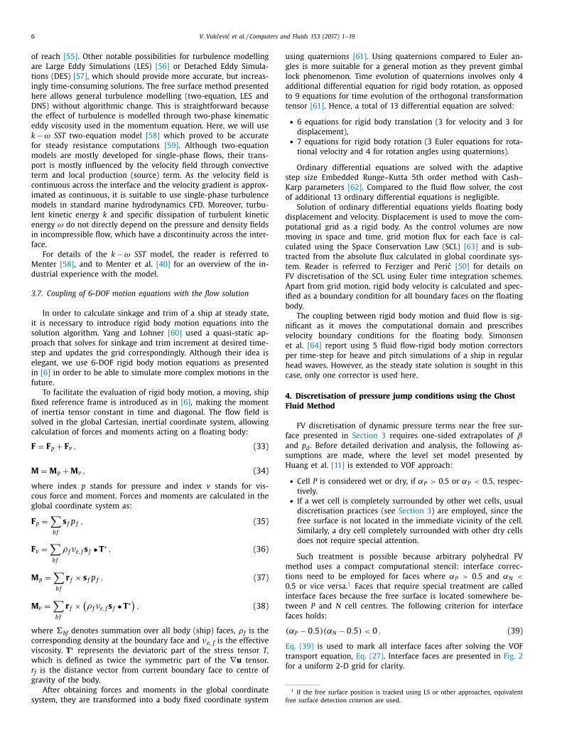
Such treatment is possible because arbitrary polyhedral FV
ethod uses a compact computational stencil: interface correc-
ions need to be employed for faces where αP > 0.5 and αN <
.5 or vice versa. 1 Faces that require special treatment are called
nterface faces because the free surface is located somewhere be-
ween P and N cell centres. The following criterion for interface
aces holds:
(αP − 0 . 5)(αN − 0 . 5) < 0 . (39)
q. (39) is used to mark all interface faces after solving the VOF
ransport equation, Eq. (27) . Interface faces are presented in Fig. 2
or a uniform 2-D grid for clarity.
V. Vuk ̌cevi ́c et al. / Computers and Fluids 153 (2017) 1–19 7
Fig. 2. Interface faces for a uniform 2-D grid. The dashed blue line denotes free sur-
face location: α = 0 . 5 . Wet cells are below the blue line: α > 0.5, while dry cells
are above the blue line: α < 0.5. Interface faces are represented with red lines. In-
terface face is a face where the free surface is located between adjacent cell centres.
Ordinary faces are denoted with black lines. (For interpretation of the references to
colour in this figure legend, the reader is referred to the web version of this article.)
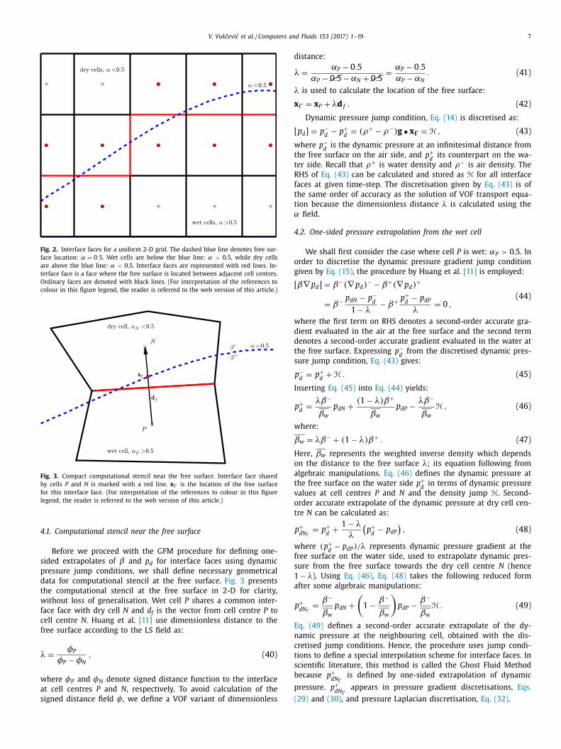
Fig. 3. Compact computational stencil near the free surface. Interface face shared
by cells P and N is marked with a red line. x � is the location of the free surface
for this interface face. (For interpretation of the references to colour in this figure
legend, the reader is referred to the web version of this article.)
4
s
p
d
t
w
f
c
f
λ
w
a
s
d
λ
λ
x
[
w
t
t
R
f
t
t
α
4
o
g
[
w
d
d
t
s
I
w
β
H
o
a
t
v
o
t
w
f
s
1
a
E
n
c
t
s
b
p
(
.1. Computational stencil near the free surface
Before we proceed with the GFM procedure for defining one-
ided extrapolates of β and p d for interface faces using dynamic
ressure jump conditions, we shall define necessary geometrical
ata for computational stencil at the free surface. Fig. 3 presents
he computational stencil at the free surface in 2-D for clarity,
ithout loss of generalisation. Wet cell P shares a common inter-
ace face with dry cell N and d f is the vector from cell centre P to
ell centre N . Huang et al. [11] use dimensionless distance to the
ree surface according to the LS field as:
=
φP
φP − φN
, (40)
here φP and φN denote signed distance function to the interface
t cell centres P and N , respectively. To avoid calculation of the
igned distance field φ, we define a VOF variant of dimensionless
istance:
=
αP − 0 . 5
αP −��0 . 5 − αN + ��0 . 5
=
αP − 0 . 5
αP − αN
. (41)
is used to calculate the location of the free surface:
� = x P + λd f . (42)
Dynamic pressure jump condition, Eq. (14) is discretised as:
p d ] = p −d
− p + d
= (ρ+ − ρ−) g • x � = H , (43)
here p −d
is the dynamic pressure at an infinitesimal distance from
he free surface on the air side, and p + d
its counterpart on the wa-
er side. Recall that ρ+ is water density and ρ− is air density. The
HS of Eq. (43) can be calculated and stored as H for all interface
aces at given time-step. The discretisation given by Eq. (43) is of
he same order of accuracy as the solution of VOF transport equa-
ion because the dimensionless distance λ is calculated using the
field.
.2. One-sided pressure extrapolation from the wet cell
We shall first consider the case where cell P is wet: αP > 0.5. In
rder to discretise the dynamic pressure gradient jump condition
iven by Eq. (15) , the procedure by Huang et al. [11] is employed:
β∇ p d ] = β−(∇ p d ) − − β+ (∇ p d )
+
= β− p dN − p −d
1 − λ− β+ p
+ d
− p dP
λ= 0 ,
(44)
here the first term on RHS denotes a second-order accurate gra-
ient evaluated in the air at the free surface and the second term
enotes a second-order accurate gradient evaluated in the water at
he free surface. Expressing p −d
from the discretised dynamic pres-
ure jump condition, Eq. (43) gives:
p −d
= p + d
+ H . (45)
nserting Eq. (45) into Eq. (44) yields:
p + d
=
λβ−
βw
p dN +
(1 − λ) β+
βw
p dP −λβ−
βw
H , (46)
here:
w
= λβ− + (1 − λ) β+ . (47)
ere, βw
represents the weighted inverse density which depends
n the distance to the free surface λ; its equation following from
lgebraic manipulations. Eq. (46) defines the dynamic pressure at
he free surface on the water side p + d
in terms of dynamic pressure
alues at cell centres P and N and the density jump H. Second-
rder accurate extrapolate of the dynamic pressure at dry cell cen-
re N can be calculated as:
p + dN �
= p + d
+
1 − λ
λ
(p +
d − p dP
), (48)
here (p + d
− p dP ) /λ represents dynamic pressure gradient at the
ree surface on the water side, used to extrapolate dynamic pres-
ure from the free surface towards the dry cell centre N (hence
− λ). Using Eq. (46) , Eq. (48) takes the following reduced form
fter some algebraic manipulations:
p + dN �
=
β−
βw
p dN +
(1 − β−
βw
)p dP −
β−
βw
H . (49)
q. (49) defines a second-order accurate extrapolate of the dy-
amic pressure at the neighbouring cell, obtained with the dis-
retised jump conditions. Hence, the procedure uses jump condi-
ions to define a special interpolation scheme for interface faces. In
cientific literature, this method is called the Ghost Fluid Method
ecause p + dN �
is defined by one-sided extrapolation of dynamic
ressure. p + dN �
appears in pressure gradient discretisations, Eqs.
29) and (30) , and pressure Laplacian discretisation, Eq. (32) .

8 V. Vuk ̌cevi ́c et al. / Computers and Fluids 153 (2017) 1–19
p
t
4
e
c
fi
4
u
w
β
w
d
o
t
t
E
e
(
w
e
r
d
t
c
4
g
v
β
w
E
4.3. One-sided pressure extrapolation from the dry cell
We shall now consider the case where cell P is dry: αP < 0.5.
Dynamic pressure jump condition, Eq. (43) is used to express p + d
:
p + d
= p −d
− H . (50)
Discretisation of the dynamic pressure gradient jump condition, Eq.
(15) yields:
β+ p dN − p + d
1 − λ− β− p −
d − p dP
λ= 0 . (51)
Comparing Eq. (51) with Eq. (44) , it can be seen that β+ and
β− are interchanged as expected. Inserting Eq. (50) into Eq.
(51) yields:
p −d
=
λβ+
βd
p dN +
(1 − λ) β−
βd
p dP +
λβ+
βd
H , (52)
where:
βd = λβ+ + (1 − λ) β− . (53)
It should be noted that βd � = βw
. Following the same procedure as
before, second-order accurate extrapolate of the dynamic pressure
at wet cell centre N can be calculated as:
p −dN �
= p −d
+
1 − λ
λ
(p −
d − p dP
). (54)
Insertion of Eq. (52) into Eq. (54) yields:
p −dN �
=
β+
βd
p dN +
(1 − β+
βw
)p dP +
β+
βw
H . (55)
Eq. (55) defines a second-order accurate extrapolate of dynamic
pressure if the cell P is dry and consequently, cell N is wet.
4.4. Summary of dynamic pressure extrapolation formulae
In the dynamic pressure extrapolation using jump conditions,
we distinguish two cases:
• Cell P is wet and cell N is dry:
p + dN �
=
β−
βw
p dN +
(1 − β−
βw
)p dP −
β−
βw
H , (56)
p −dP �
=
β+
βw
p dP +
(1 − β+
βw
)p dN +
β+
βw
H , (57)
• Cell P is dry and cell N is wet:
p −dN �
=
β+
βd
p dN +
(1 − β+
βd
)p dP +
β+
βd
H , (58)
p + dP �
=
β−
βd
p dP +
(1 − β−
βd
)p dN −
β−
βd
H . (59)
Eqs. (57) and (59) are derived in analogy to Eqs. (56) and (58) ,
looking from cell N to cell P . Eqs. (56) –(59) need further com-
ments. In OpenFOAM, cell P is denoted as owner of neighbour-
ing cell N , depending on the direction of the face normal. Conse-
quently, cell P may be wet or dry, leading to expressions for:
• p + dN �
– used when P is wet ( N is dry) for discretisation looking
from cell P ; • p −
dP �– used when P is wet ( N is dry) for discretisation looking
from cell N ; • p −
dN �– used when P is dry ( N is wet) for discretisation looking
from cell P ; • p +
dP �– used when P is dry ( N is wet) for discretisation looking
from cell N .
Eqs. (56) and (57) will be used to prove the symmetry of the
ressure Laplacian in Eq. (32) , which is a natural consequence of
he incompressibility condition.
.5. Notes on density extrapolation
Face interpolated density in the pressure equation, Eq. (32) is
xtrapolated as follows:
• Looking from the wet cell:
(β) f � = β+ , (60)
• Looking from the dry cell:
(β) f � = β− . (61)
Simple expressions for face interpolated densities are also a
onsequence of the incompressibility condition, where the density
eld is assumed constant in a given fluid.
.6. Interface contribution in the discretised Gauss pressure gradient
To demonstrate the effect of interface corrections on the eval-
ation of the Gauss gradient, we inspect the case where cell P is
et in detail. Eq. (29) can be written in the following form:
P �p dP =
βP
V P
∑
f ��s f ( f x p dP + (1 − f x ) p dN )
+
βP
V P
∑
f�
s f (
f x p dP + (1 − f x ) p + dN �
), (62)
here ∑
f ��denotes summation over non-interface faces and f �
enotes summation over interface faces. The first sum on the RHS
f Eq. (62) does not need special attention: ordinary interpola-
ion scheme is sufficient. Furthermore, if cell P is wet ( αP > 0.5),
hen βP = β+ . For interpolation on interface faces (second sum in
q. (62) ), p + dN �
is used because cell P is wet (+). We proceed to
xamine interface contributions in the second sum. Inserting Eq.
56) into second sum in Eq. (62) yields:
βP
V P
∑
f�
s f (
f x p dP + (1 − f x ) p + dN �
)=
1
V P
∑
f�
s f β+ p dP
+
1
V P
∑
f�
s f β+ β−
βw
(1 − f x )(p dN − p dP − H) ,
(63)
here the first term on the RHS can be identified as first order
xtrapolation. The second term represents the second order cor-
ection arising from discretisation of dynamic pressure jump con-
itions via GFM. Eq. (63) represents interface correction contribu-
ions for interface faces when the cell is wet. Similar expression
an be obtained for dry cell using p −dN �
given by Eq. (58) .
.7. Interface contribution in the discretised least squares pressure
radient
Least squares gradient discretisation for wet cell P , Eq. (30) , di-
ided into two sums reads:
P �p dP =
βP
V P
∑
f ��l f ( p dN − p dP )
+
βP
V P
∑
f�
l f (
p + dN �
− p dP
), (64)
here l f = w
2 f G
−1 • d f . Inserting Eq. (56) into the second sum in
q. (64) yields:
βP
V P
∑
f�
l f (
p + dN �
− p dP
)=
∑
f�
l f β+ β−
βw
(p dN − p dP − H) , (65)

V. Vuk ̌cevi ́c et al. / Computers and Fluids 153 (2017) 1–19 9
w
4
S
s
t
w
E
a
r
w
(
(
w
t
c
d
U
i
a
F
p
S
W
s
(
w
c
a
d
L
P
a
C
t
o
f
S
I
d
m
t
d
a
p
a
a
d
w
i
5
s
P
u
P
l
t
t
f
d
f
t
s
s
E
d
d
u
v
e
6
o
r
l
a
s
t
o
w
t
c
n
t
c
s
v
p
here βP = β+ has been used because cell P is considered wet (+).
.8. Interface contribution in the discretised pressure Laplacian
Detailed inspection of the pressure equation, Eq. (25) in
ection 3.3 led to conclusion that interface corrected interpolation
chemes should produce a symmetric matrix. The implicit part of
he pressure equation, Eq. (32) can be divided into two sums:
∑
f
(1
a P
)f
(β) f � | s f | (p dN − p dP ) �
| d f |
=
∑
f ��
(1
a P
)f
(β) f | s f | p dN − p dP
| d f |
+
∑
f�
(1
a P
)f
(β) f � | s f | p +
dN �− p dP
| d f | , (66)
here wet owner cell P is considered. The first sum on the RHS of
q. (66) denotes fully wet or fully dry faces: interface corrections
re not needed and the resulting matrix contributions are symmet-
ic as in single-phase flows. Consider a contribution for a single
et owner cell P and dry neighbour cell N pair, by inserting Eq.
56) into Eq. (66) :
1
a P
)f
(β) f � | s f | p +
dN �− p dP
| d f | =
(1
a P
)f
| s f | | d f |
β+ β−
βw
( p dN − p dP − H ) ,
(67)
here (β) f � = β+ because cell P is considered wet. Diagonal con-
ribution in discretisation of pressure Laplacian at an interface face
an be identified as:
P = −(
1
a P
)f
| s f | | d f |
β+ β−
βw
. (68)
pper matrix coefficient accounting for the influence of neighbour-
ng cell N to cell P is:
PN =
(1
a P
)f
| s f | | d f |
β+ β−
βw
. (69)
urthermore, additional source term is present on the RHS of the
ressure equation due to discretisation of jump conditions:
P =
(1
a P
)f
| s f | | d f |
β+ β−
βw
H . (70)
e now proceed to inspect interface face contribution to the pres-
ure equation for the neighbouring cell N :
1
a P
)f
(β) f � | s f | p −
dP �− p dN
| d f | =
(1
a P
)f
| s f | | d f |
β+ β−
βw
( p dP − p dN + H ) ,
(71)
here Eq. (57) for p −dP �
is used and (β) f � = β− because cell N is
onsidered dry. Diagonal contribution for cell N can be identified
s:
N = −(
1
a P
)f
| s f | | d f |
β+ β−
βw
. (72)
ower matrix coefficient accounting for the influence of owner cell
to cell N is:
NP =
(1
a P
)f
| s f | | d f |
β+ β−
βw
. (73)
omparison of the upper matrix coefficient given by Eq. (69) and
he lower matrix coefficient given by Eq. (73) proves the symmetry
f the matrix, as postulated in Section 3.3 . Additional source term
or cell N is:
N = −(
1
a P
)f
| s f | | d f |
β+ β−
βw
H . (74)
t is important to note that additional source terms arising from
ynamic pressure jump conditions at interface faces are antisym-
etric (see Eqs. (70) and (74) ). The source terms represent addi-
ional flux through the interface face that will be balanced by the
ynamic pressure jump after solving the pressure equation. Equiv-
lent properties can be easily derived for dry cell P and wet cell N
air.
By inspecting Eqs. (68) and (69) , we stress that the matrix di-
gonal can be reconstructed using off-diagonal matrix coefficients
s:
P = −∑
f
a PN , (75)
here f is the summation over all neighbours of cell P , both for
nterface faces and non-interface faces.
. Segregated solution algorithm
The flow chart of the segregated solution algorithm is pre-
ented in Fig. 4 . The solution algorithm is a combination of SIM-
LE [42] and PISO [43] algorithms. The SIMPLE loop handles α − − p d coupling with the rigid body motion, while the embedded
ISO loop is used to further resolve u − p d coupling. The SIMPLE
oop starts by calculating the 6-DOF rigid body motion, updating
he mesh and relative fluxes and solving the VOF transport equa-
ion, Eq. (27) . After obtaining a new estimate of the α field, inter-
ace faces are marked in order to prepare for discretisation of the
ynamic pressure terms in mixture equations, see Section 4 . Ef-
ective viscosity of the two phases is updated using Eq. (4) before
he mixture momentum equation. The PISO loop starts with the
olution of momentum equation, Eq. (19) , using the dynamic pres-
ure from the previous iteration. The dynamic pressure equation,
q. (25) is formulated and solved, taking into account pressure–
ensity coupling through GFM treatment of interface jump con-
itions. New dynamic pressure with jumps across the interface is
sed to correct the velocity field, making the face flux field conser-
ative, Eq. (26) . On convergence of the PISO loop, turbulence model
quations are solved and the effective viscosity νe is updated.
. Test cases
As the mathematical model is exact for inviscid flow with-
ut surface tension, an inviscid 2-D free surface flow over a
amp [65] is considered first, where the water height at the out-
et boundary is compared with the analytical solution. Simulations
re carried out using sets of block-structured hexahedral and un-
tructured prismatic grids in order to compare numerical uncer-
ainties. Furthermore, a simple hydrostatic test case is performed
n a block-structured grid in order to discuss spurious velocities
hich can be observed when using conditionally averaged equa-
ions and segregated solution algorithms.
The second set of test cases considers steady resistance of a
ontainer ship with dynamic sinkage and trim for different Froude
umbers. Four unstructured computational grids are used and de-
ailed verification is performed for all Froude numbers. Results are
ompared to experimental data published at the Tokyo 2015 Work-
hop website [66–68] . Along with iterative and grid uncertainties,
alidation uncertainties are calculated for all conditions, as the ex-
erimental uncertainty is readily available [66] .

10 V. Vuk ̌cevi ́c et al. / Computers and Fluids 153 (2017) 1–19
Fig. 4. Flow chart of the segregated solution algorithm.
t
a
t
(
w
o
6
r
f
C
t
ε
b
w
g
g
a
t
r
a
b
r
d
v
w
t
o
e
m
U
w
δ
w
g
(
l
H
t
U
w
t
v
t
U
c
m
6.1. Discretisation and numerical settings
Time derivative terms are discretised using the first order ac-
curate implicit Euler scheme [49,50] , convective term in the mo-
mentum equation is discretised with second order accurate linear
upwind scheme, while the convective term in the VOF equation
is discretised with second order accurate Total Variation Diminish-
ing (TVD) [69] scheme with van Leer’s flux limiter [70] in a de-
ferred correction formulation [50] . Pressure gradient term in the
momentum equation is discretised using the second order accu-
rate least squares scheme with interface jump correction relying on
the GFM. Pressure Laplacian in the pressure equation is discretised
with second order central differencing scheme with interface cor-
rection, using the over-relaxed approach for non-orthogonal cor-
rection [38,51] . Since all spatial discretisation schemes are second
order accurate, second order grid refinement convergence is ex-
pected.
All governing equations are solved with Krylov subspace linear
system solvers [71] . Symmetric pressure equation is solved with
he Conjugate gradient method [72] using Cholesky factorisation
s a preconditioner. Non-symmetric momentum and volume frac-
ion equations are solved with Stabilised Bi-Conjugate Gradient
BiCGStab) [73] method with Incomplete L-U (ILU) preconditioner
ithout fill in [71] . Under-relaxation [42] factors not used unless
therwise stated.
.2. Outline of validation and verification procedures
In order to validate the implemented methodology, simulations
esults shall be compared with analytical and experimental data
or first and second test case, respectively. The relative error of the
FD solution S CFD compared to the analytical or experimental solu-
ion S is defined as:
=
S − S CF D
S , (76)
The order of grid convergence is calculated following guidelines
y Versteeg and Malalasekera [49] based on work by Roache [74] :
p G =
ln
(S f −S m S m −S c
)ln (r G )
, (77)
here p G is the achieved order of spatial accuracy, S c is the coarse
rid solution, S m
is the medium grid solution and S f is the fine
rid solution. r G is the grid refinement ratio, which should prefer-
bly be constant. As the constant grid refinement ratio is difficult
o achieve using unstructured grids, the average grid refinement
atio between coarse/medium and medium/fine grids is used. We
lso stress that one of the Roache’s [74] conditions for Eq. (77) to
e valid states that the flow field must be sufficiently smooth. This
equirement is not met as the dynamic pressure and density have a
iscontinuity across the free surface. However, since the grid con-
ergence of integral quantities shall be assessed in present work,
e assume Eq. (77) to be valid even though the integral quanti-
ies ( i.e. force on the ship’s hull) are obtained using discontinu-
us density and pressure fields. Following guidelines given by Stern
t al. [75] , Richardson extrapolation (RE) is used to calculate nor-
alised grid uncertainty:
G =
U G
| S f | =
δRE
| S f | , (78)
here S f is the finest grid solution and δRE is the grid error:
RE =
∣∣εG m, f
∣∣r | p G | G
− 1
, (79)
here εG m, f = S f − S m
is the difference between fine and medium
rid solutions.
It is important to note that grid uncertainty calculated with Eq.
78) is valid only if monotone convergence is achieved. For oscil-
atory grid convergence, order of accuracy cannot be calculated.
owever, following Stern et al. [75] , grid uncertainty may be es-
imated as:
G =
U G
| S f | =
1
2
| S max − S min | | S f | , (80)
here S max and S min are the maximum and minimum solutions ob-
ained from a set of coarse, medium and fine grids.
Finally, if neither monotonically converging or oscillatory con-
erging solutions are obtained with grid refinement, grid uncer-
ainty is estimated following Simonsen et al. [64] :
G =
U G
| S f | =
| S max − S min | | S f | , (81)
alculating the grid uncertainty as the absolute value of the maxi-
um and minimum solutions.

V. Vuk ̌cevi ́c et al. / Computers and Fluids 153 (2017) 1–19 11
Fig. 5. Representative signal of trim convergence for the KCS ship in calm sea at
F r = 0 . 282 (case 6).
t
i
o
U
w
i
U
t
t
F
u
z
t
b
e
U
w
v
s
h
Fig. 6. Geometry of the computational domain for the 2-D ramp test case.
Table 1
Simulation parameters for the 2-D
ramp test case [76] .
Item Value
ρh , kg/m
3 1
ρ l , kg/m
3 0.001
g , m/s 2 [0 , −9 . 81 , 0]
h 1 , m 1
u , m/s [6, 0, 0]
F r = | u | / √ | g | h 1 1.92
Table 2
Boundary conditions for the 2-D ramp test
case.
Inlet Outlet Bottom Top
u f.v. z.g. s. s.
p d z.g. z.g. z.g. f.v.
α f.v. z.g. z.g. z.g.
a
u
ε
m
s
6
v
i
a
fi
u
c
t
A
i
t
S
t
w
u
c
b
b
A
c
f 1
For the steady resistance test cases, experimental data uncer-
ainty U D is reported in [66] for all Froude number conditions
n percentages of measured values. Hence, it is possible to assess
verall validation uncertainty as:
V =
√
U
2 D
+ U
2 SN
, (82)
here U SN is the simulation numerical uncertainty calculated from
terative uncertainty U I and grid uncertainty U G :
SN =
√
U
2 I
+ U
2 G
. (83)
Convergence of the drag force coefficient, sinkage and trim in
ime is observed to be oscillatory for the steady resistance simula-
ions. Fig. 5 presents the oscillatory convergence of trim for largest
roude number condition. Fig. 5 (a) presents trim signal from sim-
lation start ( t = 0 s) to end ( t = 100 s), while Fig. 5 (b) presents
oomed convergence from t = 40 s to end of simulation. Although
he convergence is oscillatory, oscillations occur within a narrow
and, indicating low iterative uncertainty. In order to quantify it-
rative uncertainty, we use the expression analogous to Eq. (80) :
I =
U I
ε f−m
=
1
2
| S I,max − S I,min | ε f−m
, (84)
here S I,max is the maximum value and S I, min is the minimum
alue. Both S I, max and S I, min are taken from last few hundred time-
teps (iterations) since small oscillations often exhibit irregular be-
aviour. As an example, Fig. 5 (b) presents illustration of τ I, max
nd τ I, min obtained from the time-evolution signal of τ . Iterative
ncertainty is always calculated based on the fine grid solution.
f−m
= S f − S m
denotes the difference between the fine and the
edium grid solution and allows U I to be represented in a dimen-
ionless form.
.3. Inviscid free surface flow over a 2-D ramp
The inviscid flow model is easily obtained by setting kinematic
iscosities of two fluids to zero. Validation for test case presented
n this section is achieved by comparing simulation results with
nalytical solution. Verification is achieved by performing grid re-
nement studies for both block-structured hexahedral grids and
nstructured prismatic grids.
Steady state flow over a 2-D ramp is a standard validation test
ase for free surface flows used by many authors [65,76] , where
he geometry of the computational domain is presented in Fig. 6 .
pplying the Bernoulli and the continuity equation for a known
nflow velocity u and free surface height h 1 , it is possible to ob-
ain the height of the free surface at the outlet boundary h 2 [76] .
imulation parameters are outlined in Table 1 .
For a general variable φ, following key words are used for cer-
ain boundary conditions:
• Zero gradient ( z.g. ): n • ∇φ = 0 . • Fixed value ( f.v. ): φ = φb . • Slip ( s. ): t • (∇u ) = 0 and n • u = 0 ,
here φb is the specified value at the boundary and t denotes
nit tangential vector. Boundaries of the computational domain in-
lude: inlet, outlet, bottom and top (see Fig. 7 ), with corresponding
oundary conditions given in Table 2 . As the flow is inviscid, slip
oundary conditions are used for velocity at the bottom boundary.
t the top, dynamic pressure is set to zero. Uniform velocity field
orresponding to the inflow velocity u and undisturbed free sur-
ace with constant height of h are used as initial conditions.

12 V. Vuk ̌cevi ́c et al. / Computers and Fluids 153 (2017) 1–19
Fig. 7. Volume fraction α at the steady state solution for four structured hexahedral
grids.
Table 3
Structured grid refinement results for 2-D ramp test case.
Index 1 2 3 4
No. cells 180 720 2 880 11 520
h 2 , m 1.03114 1.07241 1.08650 1.08662
ε, % 5.38 1.59 0.30 0.29
Fig. 8. Volume fraction α at the steady state solution for four unstructured pris-
matic grids.
Table 4
Unstructured grid refinement results for 2-D
ramp test case.
Index 1 2 3
No. cells 2 892 13 913 26 112
h 2 , m 1.02634 1.09777 1.09250
ε, % 5.82 −0.73 −0.25
6
d
s
a
r
v
o
i
t
t
c
g
o
g
6
d
a
s
d
s
r
C
b
6.3.1. Refinement study with block-structured hexahedral grids
The initial, coarsest grid consists of 15 × 12 = 180 cells, shown
in Fig. 7 (a). Grading of cells in longitudinal direction towards the
ramp and in the vertical direction towards the undisturbed free
surface is used. A constant grid refinement ratio [74] r G = 2 is
applied three times, producing three additional grids consisting
of 720, 2 880 and 11,520 cells. Steady state solution for each of
four grids is presented in Fig. 7 . The computed free surface height
at the outlet boundary is compared with the analytical solution
h 2 a = 1 . 08973 m [76] for all grids. Table 3 presents the solution
for four grids and corresponding relative errors calculated with Eq.
(76) .
Taking into account three coarsest grids (1, 2 and 3), achieved
order of spatial accuracy is p G = 1 . 55 , while taking into account
three finest grids (2, 3 and 4) results in p G = 6 . 87 . The unrealisti-
cally high order of convergence using three finest grids is due to
the fact that the solutions are not within asymptotic range of con-
vergence, as calculated using the Grid Convergence Index follow-
ing guidelines presented in [77] . Taking into account three coars-
est grids (1, 2 and 3), grid uncertainty is U G = 0 . 67% , while for the
three finest grids U ≈ 10 −4 % .
G.3.2. Refinement study with unstructured prismatic grids
Three grids with prisms (extruded triangles in the third,
ummy direction) are used for the unstructured grid refinement
tudy. The coarse, medium and fine grids consist of 2892, 13,913
nd 26,112 cells, respectively, leading to an average grid refinement
atio r G ≈ 1.78. Fig. 8 presents the steady-state α field and provides
isual details of the grids. Table 3 presents the water height at the
utlet for the three grids and corresponding relative errors.
Although the relative errors using unstructured grids reported
n Table 4 are similar to the relative errors obtained with struc-
ured grids, monotone convergence is not achieved for unstruc-
ured grids. The achieved order of spatial accuracy cannot be cal-
ulated, thus, we proceed to inspect grid uncertainties. Calculating
rid uncertainties using Eq. (80) for oscillatory convergence, we
btain U G = 3 . 3% , which is higher than in the case of structured
rids.
.3.3. Spurious air velocities in hydrostatic test case
As indicated in Section 1.3 , the numerical model using con-
itionally averaged momentum equation with segregated solution
lgorithms yields spurious air velocities. Specifically, the cause of
purious air velocities can be directly linked to the pressure–
ensity coupling being resolved in the momentum equation. We
tress that this numerical phenomena is unrelated to parasitic cur-
ents caused by numerical issues in atomisation calculations due to
ontinuous Surface Stress (CSS) model [46] . This is demonstrated
y considering the inviscid case without surface tension effects.

V. Vuk ̌cevi ́c et al. / Computers and Fluids 153 (2017) 1–19 13
s
s
w
s
i
e
g
t
s
o
a
t
t
h
F
m
a
m
a
s
t
s
t
t
m
v
a
i
a
fi
t
A
t
t
d
b
c
c
h
s
6
a
s
r
t
t
o
a
r
w
a
o
s
t
t
6
t
r
Fig. 9. Air velocities near the free surface for the hydrostatic test case.
fl
s
i
s
n
t
s
t
t
i
To test the improvements using the present approach, we con-
ider the hydrostatic variant of this test case where the calm free
urface is initialised and the velocity field is set to zero every-
here. Such hydrostatic test case is linear, hence the converged
olution should be obtained in a single time-step. OpenFOAM’s
nterFoam multiphase flow solver is based on conditionally av-
raged equations and is used for comparison. Additional details re-
arding the interFoam solver can be found in numerous publica-
ions [25–29] . To further stress the inconsistency, we use the fine
tructured hexahedral mesh.
As the considered problem is linear, a single time-step with
ne pressure correction step has been computed. Velocity fields
fter the momentum equation (momentum predictor step) and af-
er the pressure correction step are compared in Fig. 9 using the
wo approaches, where we stress that the different velocity scales
ave been used for each figure in order to visualise the difference.
ig. 9 (a) presents the velocity field after the solution of the mo-
entum equation using the conditional averaging approach, where
single layer of cells in air adjacent to the free surface has velocity
agnitudes up to O(10 3 ) . The extreme velocities in the intermedi-
te step of the solution algorithm are caused by the dynamic pres-
ure and density (free surface) imbalance in the momentum equa-
ion. In the present approach, the dynamic pressure–density (free
urface) coupling is resolved in the pressure equation, indicating
hat there should be no spurious air velocities after the momen-
um predictor step. This is demonstrated in Fig. 9 (b), where the
aximum velocity is O(10 −5 ) due to discretisation errors. The final
elocity field after the pressure correction step using conditional
veraging approach yields velocity magnitudes of O(10 −3 ) , which
s 7 orders of magnitude smaller than the velocity field obtained
fter the momentum predictor step. In contrast, the final velocity
eld using the present approach is the same as after the momen-
um predictor step, as can be seen by comparing Fig. 9 (d) and (b).
lthough the maximum velocity magnitude obtained with condi-
ionally averaged approach is reduced by 7 orders of magnitude in
he pressure correction step, the final maximum value is two or-
ers of magnitude smaller in the present approach. It should also
e noted that the velocity field of O(10 −5 ) in the present approach
an be observed both in air and water (indicating the level of dis-
retisation errors), while in the conditionally averaged approach,
igher velocities can be found only in air cells adjacent to the free
urface.
.3.4. Summary of the results
For the 2-D ramp test case, both block-structured hexahedral
nd unstructured prismatic grids have been used. For the block-
tructured hexahedral grids, the achieved order of spatial accu-
acy for the water height at the outlet is 1.55 considering first
hree grids and 6.87 considering last three grids (where the solu-
ions are not within asymptotic range of convergence). The results
n unstructured grids exhibit oscillatory convergence, hence, the
chieved order of spatial accuracy could not be determined. The
esults on both structured and unstructured grids compare well
ith the analytical solution. For comparison with the condition-
lly averaged equations, a simple hydrostatic test case is carried
ut using the same geometry, where it was demonstrated that the
purious air velocities (related to density–pressure coupling inside
he momentum equation using segregated solution algorithm, not
he surface tension effects) are remedied with present approach.
.4. Simulations of a Kriso (Moeri) container ship in calm seas
Steady resistance of a ship in calm seas is one of standard
est cases for validation and verification of a viscous CFD algo-
ithm, as used by many authors [11,39,60,78] . Viscous free-surface
ow around the KCS model free to sink and trim will be con-
idered. KCS is a modern container ship investigated both exper-
mentally [79,80] and numerically [81] , and is one of the three
hips used for Tokyo 2015 Workshop on CFD in Ship Hydrody-
amics [66] . Experimental data concerning resistance, sinkage and
rim, along with the data uncertainty is available at the Work-
hop’s website [66] . Main particulars of the ship for sinkage and
rim results are briefly given in Table 5 , while the reader is referred
o [66] for additional details. Longitudinal centre of buoyancy LCB
s 1.48% L from mid-ship towards aft of the ship.
PP
14 V. Vuk ̌cevi ́c et al. / Computers and Fluids 153 (2017) 1–19
Table 5
Main particulars of the KCS model [66] .
Item Units Value
Length between perpendiculars L PP , m 7.2786
Maximum beam of waterline B WL , m 1.0190
Depth D , m 0.6013
Draft T , m 0.3418
Displacement ∇ , m
3 1.6490
Wetted surface coefficient S W /L 2 PP 0.1803
Block coefficient C B 0.6505
Pitch radius of inertia r y , m 1.81965
Fig. 10. Coarse KCS grid details.
ω
r
i
r
l
6
A
Experimental settings are: g = 9 . 81 m/s 2 , ρw
= 999 . 5 kg/m
3 and
νw
= 1 . 27 · 10 −6 m
2 /s. The model is free to sink (translation in ver-
tical direction) and trim (rotation around transversal axis), and 6
conditions given in Table 6 are considered, where:
F r =
U √
gL PP
, (85)
is the Froude number. The Reynolds number is given as:
R e =
UL PP
νw
, (86)
where U is the forward speed of the model.
6.4.1. Unstructured computational grids
Four unstructured, polyhedral FV grids are used. The origin of
the coordinate system is located at mid-ship in the longitudinal
direction and at calm water in the vertical direction. Symmetry
plane is used to decrease cell count and consequently computa-
tional cost. x axis is positive from aft to fore perpendicular of the
ship, while y axis is positive towards portside of the ship. z axis is
positive upwards, defining a right-handed coordinate system. The
bounding box of the computational domain is: x ∈ [ −21 . 8 , 10 . 9] ,
y ∈ [0, 11.4] and z ∈ [ −11 . 8 , 8 . 2] meters. Since grids are unstruc-
tured, it is difficult to achieve constant grid refinement ratio. Four
grids consist of approximately 60 0,0 0 0, 950,0 0 0, 2,60 0,0 0 0 and
4,60 0,0 0 0 cells, and their details are given in Table 7 . Grid refine-
ment ratio, r G = 1 . 28 , is calculated as the average of successive
grid refinement ratios and is used in the grid convergence study.
We note that relatively coarse grids are used with low grid refine-
ment ratios due to limited computational resources. Details of the
coarse grid are presented in Fig. 10 .
6.4.2. Boundary conditions and numerical settings for KCS cases
Each grid has the following set of boundaries: inlet, outlet, bot-
tom, atmosphere, far-field, hull and symmetry plane. Correspond-
ing boundary conditions are given in Table 8 . u ship denotes the
specified forward speed of the ship, while u wall denotes moving
wall velocity as calculated from the 6-DOF solution. αswl corre-
sponds to the volume fraction distribution according to still water
level. Inlet–outlet (mixed) boundary condition is used at the bot-
tom and atmosphere for α: zero gradient is used if outflow occurs,
fixed value of 0 and 1 is used otherwise for atmosphere and bot-
tom, respectively. Free stream values of k and ω are calculated and
imposed on the inlet, while wall functions are used at the hull. Im-
plicit relaxation zones [82] are used at the inlet, outlet and far-field
boundaries.
The following initial conditions are used: uniform velocity field
u = u ship , α distribution corresponding to still water level obtained
with cell cutting algorithm, uniform dynamic pressure p d = 0 , uni-
form turbulent kinetic energy k = k f s and uniform specific dissipa-
tion of turbulent kinetic energy ω = ω f s .
Grid motion, k and ω under-relaxation parameters are set to
0.5 and the under-relaxation parameter for velocity field is set
to 0.7. Grid motion is under-relaxed explicitly, while u , k and
are under-relaxed implicitly [42] . α and p d are not under-
elaxed. Under-relaxation parameter of 0.5 for grid motion slightly
mproves convergence of sinkage and trim compared to under-
elaxation parameter of 1 which causes a more pronounced oscil-
atory behaviour.
.4.3. Computational results for the KCS model in calm seas
Computations for 6 conditions given in Table 6 are carried out.
t steady state, drag force coefficient C , sinkage σ and trim τ are
T
V. Vuk ̌cevi ́c et al. / Computers and Fluids 153 (2017) 1–19 15
Table 6
Steady resistance conditions for the KCS model [66] .
Index i 1 2 3 4 5 6
Forward speed U , m/s 0.915 1.281 1.647 1.922 2.196 2.379
Froude number F r 0.108 0.152 0.195 0.227 0.260 0.282
Reynolds number R e · 10 −6 5.23 7.33 9.42 1.10 1.26 1.36
Table 7
Computational grids for the KCS model.
Grid index 1 2 3 4
Number of cells 607 114 954 016 2 643 763 4 661 889
Hexahedral cells 535 096 853 998 2 422 245 4 331 549
Prismatic cells 23 933 33 430 77 582 118 077
Polyhedral cells 44 599 61 565 132 118 194 026
Maximum non-orthogonality, ° 84.3 75.2 86.8 76.1
Average non-orthogonality, ° 8.5 7.5 7.5 6.6
Maximum aspect ratio 807 787 656 779
Table 8
Boundary conditions for the KCS test case.
Inlet Outlet Bottom Atmosphere Far-field Hull
u u ship Pressure outlet Zero gradient u wall
p d zero gradient Fixed value Zero gradient
α αswl Inlet–outlet Zero gradient
k k fs Zero gradient Wall function
ω ω fs Zero gradient Wall function
c
fi
C
w
t
b
t
g
F
w
i
p
t
6
fi
i
i
I
a
0
F
s
a
g
g
c
l
o
s
r
n
t
Table 9
Validation and verification: F r = 0 . 108 case.
Measured parameters C T · 10 3 σ , cm τ , °
Experimental results S 3.796 −0.090 −0.017
Grid 1 solution S 1 4.242 −0.200 −0.035
Grid 2 solution S 2 4.141 −0.194 −0.034
Grid 3 solution S 3 3.972 −0.188 −0.030
Absolute error 1 E 1 −0.446 0.110 0.018
Absolute error 2 E 2 −0.345 0.104 0.017
Absolute error 3 E 3 −0.175 0.098 0.013
Relative error 1 ε1 , % −11.8 −122.1 −106.1
Relative error 2 ε2 , % −9.1 −115.6 −97.2
Relative error 3 ε3 , % −4.6 −109.0 −74.8
Iterative uncertainty U I −9 . 36 · 10 −3 1 . 98 · 10 −5 4 . 62 · 10 −6
Order of accuracy p G N/A N/A N/A
Grid uncertainty U G , % 6.8 6.4 16.7
Data uncertainty U D , % 1.0 8.2 9.6
Validation uncertainty U V 0.2730 0.0196 0.0058
t
c
a
b
w
0
I
u
t
f
p
a
f
f
r
l
t
b
alculated and compared to experimental results. Drag force coef-
cient is calculated as:
T =
| F x | 0 . 5 ρw
U
2 S W
, (87)
here F x is the fluid force acting on a ship hull in the longi-
udinal direction. Sinkage and trim are readily available as rigid
ody translation in the vertical direction and rotation around the
ransversal axis.
Fig. 11 shows the comparison of CFD results on the finest
rid (4,60 0,0 0 0 cells) and experimental results over a range of
roude numbers. Fig. 11 (a) presents the drag force coefficient,
hile Fig. 11 (b) and (c) shows sinkage and trim, respectively. C T s dimensionless, σ is presented in centimetres for clarity and τ is
resented in degrees. CFD results show good agreement compared
o experimental results.
.4.4. Verification and validation study
Verification and validation results corresponding to the grid re-
nement study for each condition given in Table 6 are presented
n Tables 9 –14 . CFD results are presented along with correspond-
ng absolute and relative errors compared to experimental results.
terative and grid uncertainties are calculated for each simulation,
nd grids 1, 2 and 3 are used for lower Froude number cases: F r = . 108 , 0 . 152 , 0 . 195 , while grids 1, 2, 3 and 4 are used for higher
roude number cases: F r = 0 . 227 , 0 . 260 , 0 . 282 .
Results for the lowest Froude number case, F r = 0 . 108 , are pre-
ented in Table 9 . Although errors for drag force coefficient, sink-
ge and trim monotonically decrease with grid refinement, conver-
ence is not achieved as the difference between fine and medium
rid solutions is larger than the difference between medium and
oarse grid solutions. Hence, order of accuracy cannot be calcu-
ated. Relative error for the drag force coefficient is less than −5%
n the fine grid, while relative errors for sinkage and trim are con-
iderably greater, −110% and −75% , respectively. Larger relative er-
ors for sinkage and trim are expected as the ship exhibits only mi-
or movement at small Froude numbers. Furthermore, experimen-
al measurement of sinkage is slightly less than −0 . 1 cm, while
he finest layer of cells near the free surface is approximately 0.5
m high. Therefore, we do not expect to correctly model sinkage
nd trim with such a coarse grid resolution for low Froude num-
ers. Taking above mentioned considerations into account along
ith the absolute errors for sinkage and trim of 0.098 cm and
.013 °, respectively, results compare well with experimental data.
terative uncertainty is low as expected, while the normalised grid
ncertainty calculated with Eq. (81) ranges from 6.4% for sinkage
o 16.7% for trim. The normalised grid uncertainty for the drag
orce coefficient is 6.8%. Overall validation uncertainties are ap-
roximately 0.27, 0.02 and 0.006 for drag force coefficient, sinkage
nd trim, respectively.
Results for the F r = 0 . 152 case are presented in Table 10 . Errors
or all measured parameters monotonically decrease. Relative error
or drag force coefficient is less than −5% for the fine grid, while
elative errors for sinkage and trim are 40% and −8% . Compared to
owest Froude number case, Table 9 , relative errors for sinkage and
rim are significantly lowered. This is expected as the same grid
etter resolves larger motions, and the measured sinkage and trim

16 V. Vuk ̌cevi ́c et al. / Computers and Fluids 153 (2017) 1–19
Fig. 11. Comparison of CFD results using the finest grid (4,60 0,0 0 0 cells) and ex-
perimental results for 6 KCS test case conditions.
Table 10
Validation and verification: F r = 0 . 152 case.
Measured parameters C T · 10 3 σ , cm τ , °
Experimental results S 3.641 −0.275 −0.053
Grid 1 solution S 1 3.972 −0.423 −0.061
Grid 2 solution S 2 3.878 −0.414 −0.059
Grid 3 solution S 3 3.819 −0.387 −0.057
Absolute error 1 E 1 −0.331 0.148 0.008
Absolute error 2 E 2 −0.237 0.139 0.006
Absolute error 3 E 3 −0.178 0.112 0.004
Relative error 1 ε1 , % −9.1 −53.7 −14.7
Relative error 2 ε2 , % −6.5 −50.4 −12.0
Relative error 3 ε3 , % −4.9 −40.4 −7.5
Iterative uncertainty U I −5 . 82 · 10 −2 1 . 05 · 10 −5 1 . 05 · 10 −5
Order of accuracy p G 1.85 N/A N/A
Grid uncertainty U G , % 2.7 9.3 7.0
Data uncertainty U D , % 1.0 5.9 6.8
Validation uncertainty U V 0.1096 0.0426 0.0056
Table 11
Validation and verification: F r = 0 . 195 case.
Measured parameters C T · 10 3 σ , cm τ , °
Experimental results S 3.475 −0.599 −0.097
Grid 1 solution S 1 3.719 −0.709 −0.107
Grid 2 solution S 2 3.691 −0.697 −0.100
Grid 3 solution S 3 3.526 −0.691 −0.102
Absolute error 1 E 1 −0.244 0.110 0.010
Absolute error 2 E 2 −0.216 0.098 0.003
Absolute error 3 E 3 −0.051 0.092 0.005
Relative error 1 ε1 , % −7.0 −18.4 −10.7
Relative error 2 ε2 , % −6.2 −16.4 −2.8
Relative error 3 ε3 , % −1.5 −15.3 −5.1
Iterative uncertainty U I −5 . 29 · 10 −2 3 . 29 · 10 −5 −1 . 69 · 10 −4
Order of accuracy p G N/A 2.57 N/A
Grid uncertainty U G , % 5.5 1.1 3.8
Data uncertainty U D , % 1.0 3.9 4.57
Validation uncertainty U V 0.1973 0.0245 0.0060
a
s
t
e
d
t
f
g
t
s
F
m
r
o
u
i
m
u
a
−
e
a
t
t
i
a
c
re approximately 3 times higher compared to F r = 0 . 108 case. Ab-
olute errors for sinkage and trim are 0.112 cm and 0.004 °. Respec-
ively, iterative uncertainties are low: ≈ 10 −2 for the drag force co-
fficient and ≈ 10 −5 for sinkage and trim. Order of accuracy for the
rag force coefficient is 1.85, giving normalised grid uncertainty es-
imate of 2.7% and validation uncertainty of approximately 0.1.
Results for the F r = 0 . 195 case are presented in Table 11 . Errors
or drag force coefficient and sinkage monotonically decrease with
rid refinement, while trim exhibits oscillatory convergence. Rela-
ive errors for the fine grid: −2% for drag force coefficient, −15% for
inkage and −5% for trim, are further lowered compared to lower
roude number cases. Iterative uncertainties are several orders of
agnitude lower than grid uncertainties. Achieved order of accu-
acy for sinkage is 2.6, giving normalised grid uncertainty estimate
f 1.1% and validation uncertainty estimate of 0.03. Normalised grid
ncertainty for oscillatory converging trim is 3.8%, followed by val-
dation uncertainty of 0.006. For the drag force coefficient, nor-
alised grid uncertainty is 5.5% with the corresponding validation
ncertainty of approximately 0.2.
Results for the F r = 0 . 227 case are presented in Table 12 . Rel-
tive errors for the drag force coefficient, sinkage and trim are:
2% , −4 . 3% and −9 . 6% on the fine grid, respectively. Drag force co-
fficient and sinkage exhibit monotone convergence with order of
ccuracy of 16 and 3.7, respectively, yielding very low grid uncer-
ainty. Iterative uncertainty for the drag force coefficient is −5 , due
o a minor difference between fine and medium grid solution. Val-
dation uncertainties for the drag force coefficient and sinkage are
pproximately 0.04 and 0.03. Trim exhibits oscillatory narrow band
onvergence which gives normalised grid uncertainty estimate of

V. Vuk ̌cevi ́c et al. / Computers and Fluids 153 (2017) 1–19 17
Table 12
Validation and verification: F r = 0 . 227 case.
Measured parameters C T · 10 3 σ , cm τ , °
Experimental results S 3.467 −0.944 −0.127
Grid 1 solution S 1 3.672 −1.008 −0.146
Grid 2 solution S 2 3.635 −0.988 −0.138
Grid 3 solution S 3 3.538 −0.987 −0.141
Grid 4 solution S 4 3.536 −0.985 −0.139
Absolute error 1 E 1 −0.205 0.064 0.019
Absolute error 2 E 2 −0.168 0.044 0.011
Absolute error 3 E 3 −0.071 0.043 0.014
Absolute error 4 E 4 −0.069 0.041 0.012
Relative error 1 ε1 , % −5.9 −6.8 −14.6
Relative error 2 ε2 , % −4.8 −4.7 −8.3
Relative error 3 ε3 , % −2.1 −4.6 −10.8
Relative error 4 ε4 , % −2.0 −4.3 −9.6
Iterative uncertainty U I −5 . 09 7 . 64 · 10 −4 5 . 04 · 10 −4
Order of accuracy p G 16.0 3.7 N/A
Grid uncertainty U G , % 0.0 0.2 1.2
Data uncertainty U D , % 1.0 2.8 3.3
Validation uncertainty U V 0.0359 0.0263 0.0044
Table 13
Validation and verification: F r = 0 . 260 case (design condition).
Measured parameters C T · 10 3 σ , cm τ , °
Experimental results S 3.711 −1.394 −0.169
Grid 1 solution S 1 3.981 −1.377 −0.174
Grid 2 solution S 2 3.910 −1.352 −0.170
Grid 3 solution S 3 3.808 −1.349 −0.169
Grid 4 solution S 4 3.726 −1.346 −0.171
Absolute error 1 E 1 −0.270 −0.017 0.005
Absolute error 2 E 2 −0.199 −0.042 0.001
Absolute error 3 E 3 −0.097 −0.045 0.0 0 0
Absolute error 4 E 4 −0.015 −0.049 0.002
Relative error 1 ε1 , % −7.3 1.3 −3.2
Relative error 2 ε2 , % −5.4 3.0 −0.9
Relative error 3 ε3 , % −2.6 3.3 −0.3
Relative error 4 ε4 , % −0.4 3.5 −1.0
Iterative uncertainty U I −3 . 15 · 10 −1 4 . 00 · 10 −3 −7 . 65 · 10 −3
Order of accuracy p G 0.86 0.13 N/A
Grid uncertainty U G , % 9.4 7.6 0.4
Data uncertainty U D , % 1.0 1.9 2.3
Validation uncertainty U V 0.3528 0.1056 0.0039
1
n
0
s
s
s
s
a
c
d
a
o
c
a
s
a
D
h
c
m
a
t
Table 14
Validation and verification: F r = 0 . 282 case.
Measured parameters C T · 10 3 σ , cm τ , °
Experimental results S 4.501 −1.702 −0.159
Grid 1 solution S 1 4.837 −1.665 −0.145
Grid 2 solution S 2 4.737 −1.650 −0.147
Grid 3 solution S 3 4.608 −1.655 −0.147
Grid 4 solution S 4 4.560 −1.653 −0.146
Absolute error 1 E 1 −0.336 −0.037 −0.014
Absolute error 2 E 2 −0.236 −0.052 −0.012
Absolute error 3 E 3 −0.107 −0.047 −0.012
Absolute error 4 E 4 −0.059 −0.049 −0.013
Relative error 1 ε1 , % −7.5 2.2 8.8
Relative error 2 ε2 , % −5.2 3.1 7.3
Relative error 3 ε3 , % −2.4 2.8 7.9
Relative error 4 ε4 , % −1.3 2.9 8.0
Iterative uncertainty U I −1 . 79 · 10 −1 2 . 59 · 10 −4 2 . 57 · 10 −3
Order of accuracy p G 3.98 N/A 6.21
Grid uncertainty U G , % 0.6 0.2 0.04
Data uncertainty U D , % 1.0 1.4 1.8
Validation uncertainty U V 0.0541 0.0233 0.0028
c
s
6
p
a
i
p
p
d
t
m
t
a
s
e
4
t
t
c
t
a
d
o
o
fi
c
t
i
o
d
r
y
6
c
t
s
w
r
a
s
c
.2%. Iterative uncertainty is low as in the previous lower Froude
umber cases, followed by low validation uncertainty estimate of
.004.
Results for the design Froude number case, F r = 0 . 260 , are pre-
ented in Table 13 . Relative errors for the drag force coefficient,
inkage and trim on the fine grid are: −0 . 4% , 3.5% and −1% , re-
pectively. As in the previous condition, drag force coefficient and
inkage exhibit monotone convergence with 0.86 and 0.13 order of
ccuracy. Achieved orders of accuracy are lower than the theoreti-
al ones, resulting in higher normalised grid uncertainties: 9.4% for
rag force coefficient and 7.6% for sinkage. Combined with low iter-
tive uncertainties, grid uncertainties yield validation uncertainties
f 0.35 (drag force coefficient) and 0.11 (sinkage). Trim exhibits os-
illatory convergence with low normalised grid uncertainty of 0.4
nd validation uncertainty of 0.004.
Results for the largest Froude number case, F r = 0 . 282 , are pre-
ented in Table 14 . Relative errors for drag force coefficient, sink-
ge and trim on the fine grid are: −1 . 3% , 2.9% and 8%, respectively.
rag force coefficient and trim exhibit monotone convergence with
igh orders of accuracy. Achieved order of accuracy for drag force
oefficient and trim are approximately 4 and 6, yielding low nor-
alised grid uncertainties of less than 1%. Iterative uncertainties
re low as in previous conditions. Resulting validation uncertain-
ies are approximately 0.05 and 0.003. Sinkage exhibits oscillatory
onvergence within narrow band. Normalised grid uncertainty for
inkage is 0.2%, yielding validation uncertainty of 0.02.
.4.5. Summary of the results
A set of steady resistance simulations with sinkage and trim is
erformed for the KCS ship model at different conditions given by
wide range of Froude numbers. Four unstructured grids are used
n order to assess grid uncertainty. Iterative uncertainties are also
resented for all conditions, and the simulation results are com-
ared to experimental data. Since the uncertainty of experimental
ata is available, validation uncertainty is assessed as well. Rela-
ive errors for the drag force coefficients on fine grids are approxi-
ately 5% for two lowest F r conditions, while the higher F r condi-
ions yield relative errors less than 2%. Relative errors for sinkage
nd trim are high for the lowest F r case as the grid resolution is in-
ufficient to capture minor ship motions. Sinkage and trim relative
rrors for higher F r conditions are within 10%.
Grid convergence for the drag force coefficient is obtained for
out of 6 conditions: 3 conditions give order of accuracy higher
han theoretical, while 1 condition gives order of accuracy lower
han theoretical. Normalised grid uncertainty is less than 3%, ex-
ept for one condition with 10%. Corresponding validation uncer-
ainties are less than 0.5. Monotone grid convergence for sink-
ge is achieved for 3 out of 6 conditions: 2 conditions yield or-
er of accuracy higher than theoretical, while 1 condition gives
rder of accuracy lower than theoretical. One condition exhibits
scillatory convergence and others do not converge with grid re-
nement, even though the errors decrease monotonically. Grid un-
ertainties for sinkage are less than 1.1%, except for one condi-
ion with 7.6%. Corresponding validation uncertainties are approx-
mately 0.03 when the grid convergence is achieved. Trim exhibits
scillatory grid convergence for 3 out of 6 conditions, while 1 con-
ition yields monotone convergence with achieved order of accu-
acy higher than theoretical. Grid uncertainties are at most 3.8%,
ielding largest validation uncertainty of 0.006.
12 out of 18 items (drag force coefficient, sinkage and trim for
conditions) exhibit convergence with grid refinement. All 6 non-
onverging items are clustered at low F r conditions which are par-
icularly challenging due to low motion magnitudes (0.09 cm for
inkage and 0.017 ° for trim at lowest Froude numbers) and small
ave elevations relative to grid resolution. We believe that better
esults could be obtained by using finer grids for low F r conditions,
lthough this is not demonstrated due to limited computational re-
ources. Moreover, it is interesting to note that the oscillatory grid
onvergence is achieved for 5 out of 12 converging items. For the

18 V. Vuk ̌cevi ́c et al. / Computers and Fluids 153 (2017) 1–19
ramp test case with block-structured grids using constant refine-
ment ratio, monotone convergence has been achieved. Observa-
tions regarding oscillatory grid convergence and grid divergence on
unstructured grids are in accordance with Larsson et al. [15] where
better grid refinement results are obtained using structured grids.
This is expected as the well controlled, uniform refinement is im-
possible with unstructured grids. However, low relative errors indi-
cate that accurate results may be obtained with unstructured grids
which are appealing for the industrial use due to easier grid gen-
eration.
7. Conclusion and future work
An implementation of the Ghost Fluid Method for free sur-
face incompressible flows in the arbitrary polyhedral Finite Volume
framework is presented in this paper. The numerical model is pre-
sented in detail, with the emphasis on the interface-corrected in-
terpolation schemes for discontinuous pressure and density fields.
Interface-corrected schemes are used only for interface faces, while
ordinary interpolation is sufficient for fully wet or dry cells. Such
treatment is straightforward because polyhedral FV method imple-
mented in OpenFOAM uses compact computational stencil. Discre-
tised Gauss gradient and least squares gradient operators for dy-
namic pressure are derived and presented. Implicit dynamic pres-
sure Laplacian operator is inspected in detail, proving the symme-
try of pressure equation. Furthermore, it follows that the diagonal
part of the pressure equation can be reconstructed using negative
off-diagonal coefficients as is the case in single-phase flow.
The verification and validation of the model is performed for
two sets of test cases: inviscid flow over a 2-D ramp and steady re-
sistance simulations of a container ship for different Froude num-
bers. The results compare well with analytical and experimental
data, while the numerical uncertainties are within reasonably low
bounds. The detailed verification and validation exercise renders
the presented method suitable for marine hydrodynamic flows.
Incorporation of the surface tension effects in the dynamic
pressure jump and the implementation of the viscous jump con-
ditions [14] should enable efficient modelling of the small scale ef-
fects, which shall be the topic of future work.
Acknowledgements
This research was sponsored by Bureau Veritas and Hyundai
Heavy Industries under the administration of Dr. Šime Malenica
and Dr. Geon-Hong Kim, whose support is gratefully acknowl-
edged. The authors express their gratitude towards Johan Rønby
and Holger Marschall for numerous helpful discussions and com-
ments. Our gratitude also goes to Mr. Marko Horvat, a graduate
student who provided the grids for the 2-D ramp test case.
References
[1] Tukovi ́c Z , Jasak H . A moving mesh finite volume interface tracking method forsurface tension dominated interfacial fluid flow. Comput Fluids 2012;55:70–84 .
[2] Dieter-Kissling K, Marschall H, Bothe D. Numerical method for coupled interfa-
cial surfactant transport on dynamic surface meshes of general topology. Com-put Fluids 2015;109:168–84. doi: 10.1016/j.compfluid.2014.12.017 .
[3] Tryggvason G, Bunner B, Esmaeeli A, Juric D, Al-Rawahi N, Tauber W, et al.A front-Tracking method for computations of multiphase flow. J Comput Phys
2001;169:708–59. doi: 10.1006/jcph.2001.6726 . [4] Stern F , Yang J , Wang Z , Sadat-Hosseini H , Mousaviraad M , Bhushan S , Xing T ,
et al. Computational ship hydrodynamics: nowadays and way forward. In: Pro-ceedings of the 29th ONR symposium on naval hydrodynamics; 2012. p. 1–73 .
[5] Luppes R , Düz B , van der Heiden H , van der Plas P , Veldman A . Numerical
simulations of two-phase flow with COMFLOW: past and recent developments.In: Proceedings of the ECCOMAS 2012 conference; 2012. p. 1–16 .
[6] Carrica PM, Wilson RV, Noack RW, Stern F. Ship motions using single-phaselevel set with dynamic overset grids. Comput Fluids 2007;36:1415–33. doi: 10.
1016/j.compfluid.2007.01.007 .
[7] Carrica PM, Wilson RV, Stern F. An unsteady single-phase level set method forviscous free surface flows. Int J Numer Meth Fluids 2007;53:229–56. doi: 10.
1002/fld.1279 . [8] Fedkiw RP , Aslam T , Xu S . The ghost fluid method for deflagration and deto-
nation discontinuities. J Comput Phys 1999;154(2):393–427 . [9] Kang M , Fedkiw RP , Liu X-D . A boundary condition capturing method for mul-
tiphase incompressible flow. J Sci Comput 20 0 0;15(3):323–60 . [10] Desjardins O , Moureau V , Pitsch H . An accurate conservative level
set/ghost fluid method for simulating turbulent atomization. J Comput
Phys 2008;227(18):8395–416 . [11] Huang J, Carrica PM, Stern F. Coupled ghost fluid/two-phase level set method
for curvilinear body-fitted grids. Int J Numer Meth Fluids 2007;44:867–97.doi: 10.1002/fld.1499 .
[12] Bo W , Grove JW . A volume of fluid method based ghost fluid method for com-pressible multi-fluid flows. Comput Fluids 2014;90:113–22 .
[13] Kaneda M , Haruna T , Suga K . Ghost-fluid-based boundary treatment in lattice
Boltzmann method and its extension to advancing boundary. Appl Therm Eng2014;72(1):126–34 .
[14] Lalanne B , Villegas LR , Tanguy S , Risso F . On the computation of viscous termsfor incompressible two-phase flows with level set/ghost fluid method. J Com-
put Phys 2015;301:289–307 . [15] Larsson L, Stern F, Visonneau M. Numerical ship hydrodynamics: an as-
sessment of the Gothenburg 2010 workshop. Springer; 2013. doi: 10.1007/
978- 94- 007- 7189- 5 . [16] Tryggvason G , Scardovelli R , Zaleski S . Direct numerical simulations of gas–liq-
uid multiphase flows. Cambridge University Press; 2011 . [17] Ubbink O , Issa RI . A method for capturing sharp fluid interfaces on arbitrary
meshes. J Comput Phys 1999;153:26–50 . [18] Ubbink O . Numerical prediction of two fluid systems with sharp interfaces,
London: Imperial College of Science, Technology & Medicine; 1997. [Ph.D. the-
sis] . [19] Rusche H . Computational fluid dynamics of dispersed two-phase flows at high
phase fractions, London: Imperial College of Science, Technology & Medicine;2002. [Ph.D. thesis] .
[20] Kissling K , Springer J , Jasak H , Schütz S , Urban K , Piesche M . A coupled pres-sure based solution algorithm based on the volume–of–fluid approach for two
or more immiscible fluids. In: Proceedings of Vth European conference on
computational fluid dynamics, ECCOMAS CFD; 2010 . [21] Sethian JA . Level set methods: evolving interfaces in geometry, fluid mechan-
ics, computer vision and materials science. Cambridge University Press; 1996 . [22] Sussman M , Smereka P , Osher S . A level set approach for computing solutions
to incompressible two-phase flow. J Comput Phys 1994;114:146–59 . [23] Olsson E , Kreiss G . A conservative level set method for two phase flow. J Com-
put Phys 2005;210(1):225–46 .
[24] Olsson E , Kreiss G , Zahedi S . A conservative level set method for two phaseflow ii. J Comput Phys 2007;225(1):785–807 .
[25] Jacobsen NG, Fuhrman DR, Fredsøe J. A wave generation toolbox for the open-source CFD library: OpenFoam®. Int J Numer Meth Fluids 2012;70(9):1073–88.
doi: 10.1002/fld.2726 . [26] Higuera P, Lara J, Losada IJ. Realistic wave generation and active wave ab-
sorption for Navier–Stokes models: application to OpenFoam®. Coast Eng2013;71:102–18. doi: 10.1016/j.coastaleng.2012.07.002 .
[27] Higuera P, Lara J, Losada IJ. Simulating coastal engineering processes with
OpenFoam®. Coast Eng 2013;71:119–34. doi: 10.1016/j.coastaleng.2012.06.002 . [28] Paulsen BT, Bredmose H, Bingham HB. An efficient domain decomposition
strategy for wave loads on surface piercing circular cylinders. Coast Eng2014a;86:57–76. doi: 10.1016/j.coastaleng.2014.01.006 .
[29] Paulsen BT, Bredmose H, Bingham HB, Jacobsen NG. Forcing of a bottom-mounted circular cylinder by steep regular water waves at finite depth. J Fluid
Mech 2014b;755:1–3. doi: 10.1017/jfm.2014.386 .
[30] Osher S , Fedkiw R . Level set methods and dynamic implicit surfaces. Springer;2003 .
[31] Sussman M , Fatemi E . An efficient, interface-preserving level set redistancingalgorithm and its application to interfacial incompressible fluid flow. SIAM J
Sci Comput 1999;20(4):1165–91 . [32] Gómez P , Hernández J , López J . On the reinitialization procedure in a nar-
row-band locally refined level set method for interfacial flows. Int J Numer
Methods Eng 2005;63:1478–512 . [33] Sun Y, Beckermann C. Sharp interface tracking using the phase-field equation.
J Comput Phys 2007;220:626–53. doi: 10.1016/j.jcp.2007.05.025 . [34] Sun Y, Beckermann C. A two-phase diffusive-interface model for Hele–Shaw
flows with large property contrasts. Physica D 2008;237:3089–98. doi: 10.1016/j.physd.2008.06.010 .
[35] Wang S, Glimm J, Samulyak R, Jiao X, Diao C. An embedded boundary method
for two phase incompressible flow. arXiv e-prints 1304.5514 ; 2013. http://adsabs.harvard.edu/abs/2013arXiv1304.5514W
[36] Johansen H, Colella P. A Cartesian grid embedding boundary method for Pois-son’s equation on irregular domains. J Comput Phys 1998;147:60–85. doi: 10.
1006/jcph.1998.5965 . [37] Crockett RK, Colella P, Graves DT. A Cartesian grid embedded boundary
method for solving the Poisson and heat equations with discontinuous coeffi-
cients in three dimensions. J Comput Phys 2010;230:613–28. doi: 10.1016/j.jcp.2010.12.017 .
[38] Jasak H . Error analysis and estimation for the finite volume method with ap-plications to fluid flows, London: Imperial College of Science, Technology &
Medicine; 1996. [Ph.D. thesis] .

V. Vuk ̌cevi ́c et al. / Computers and Fluids 153 (2017) 1–19 19
[
[
[
[
[
[
[
[
[
[
[
[
[
[
[
[
[
[
[
[
[
[
[
[
[
[
[
[
[
[
[
39] Queutey P, Visonneau M. An interface capturing method for free–surface hy-drodynamic flows. Comput Fluids 2007;36:1481–510. doi: 10.1002/j.compfluid.
20 06.11.0 07 . 40] Menter FR , Kuntz M , Langtry R . Ten years of industrial experience with the SST
turbulence model. Turbul Heat Mass Transf 2003;4:625–32 . [41] Weller HG , Tabor G , Jasak H , Fureby C . A tensorial approach to computa-
tional continuum mechanics using object oriented techniques. Comput Phys1998;12:620–31 .
42] Patankar SV , Spalding DB . A calculation procedure for heat, mass and mo-
mentum transfer in three-dimensional parabolic flows. Int J Heat Mass Transf1972;15:1787–806 .
43] Issa RI . Solution of the implicitly discretised fluid flow equations by opera-tor-splitting. J Comput Phys 1986;62:40–65 .
44] Batchelor FR . An introduction to fluid dynamics. Cambridge University Press;1967 .
45] Dopazo C . On conditional averages for intermittent turbulent flows. J Fluid
Mech 1977;81:433–8 . 46] Ashgriz N . Handbook of atomization and sprays: theory and applications.
Springer Science & Business Media; 2011 . [47] Wilcox DC . Turbulence modeling for CFD. DCW Industries; 1993 .
48] Ito K, Li Z. Interface conditions for Stokes equations with a discontinuous vis-cosity and surface sources. Appl Math Lett 2006;19:229–34. doi: 10.1016/j.aml.
2005.02.041 .
49] Versteeg HK , Malalasekera W . An introduction to computational fluid dynam-ics: the finite volume method. Pearson Education Limited; 1995 .
50] Ferziger JH , Peric M . Computational methods for fluid dynamics. Springer;1996 .
[51] Demirdži ́c I. On the discretization of the diffusion term in finite–volume con-tinuum mechanics. Numer Heat Transf B 2015;68:1–10. doi: 10.1080/10407790.
2014.985992 .
52] Rhie CM , Chow WL . A numerical study of the turbulent flow past an isolatedairfoil with trailing edge separation. AIAA J 1983;21:1525–32 .
53] Vuk ̌cevi ́c V , Östman A , Jasak H . Rapid simulations of pure sway motion usingFVM in OpenFOAM. In: Proceedings of workshop on verification and validation
of ship manoeuvring simulation methods (SIMMAN 2014); 2014 . 54] Jasak H , Weller HG . Application of the finite volume method and unstructured
meshes to linear elasticity. Int J Numer Methods Eng 20 0 0;48:267–87 .
55] Specialist committee on CFD in marine hydrodynamics. Final report and rec-ommendations to the 27th ITTC. Proceedings of the 27th International Towing
Tank Conference Aug.–Sep. 2014 [available online; accessed 20.08.15]. 56] Pereira FS , Vaz G , Eca L . On the numerical requirements of RANS and hy-
brid turbulence models. In: Proceedings of the MARINE 2015 conference; 2015.p. 886–902 .
[57] Li D , Hallander J , Johansson T , Karlsson R . Cavitation dynamics and underwater
radiated noise signature of a ship with a cavitating propeller. In: Proceedingsof the MARINE 2015 conference; 2015. p. 401–12 .
58] Menter FR . Two-equation eddy-viscosity turbulence models for engineeringapplications. AIAA J 1994;32(8):1598–605 .
59] Jasak H , Vuk ̌cevi ́c V , Christ D . Rapid free surface simulation for steady-statehull resistance with FVM using OpenFOAM. In: Proceedings of the 30th sym-
posium on naval hydrodynamics; 2014. p. 548–54 . 60] Yang C , Löhner R . Calculation of ship sinkage and trim using a finite element
method and unstructured grids. Int J CFD 2002;16(3):217–27 .
[61] Coutsias EA , Romero L . The quaternions with an application to rigid body dy-namics. Department of Mathematics and Statistics 1999 .
62] Press WH , Teukolsky SA , Vetterling WT , Flannery BP . Numerical recipes in C++:the art of scientific computing. Cambridge University Press; 2002 .
63] Demiridži ́c I, Peri ́c M. Space conservation law in finite volume calculationsof fluid flow. Int J Numer Methods Fluids 1988;8:1037–50. doi: 10.1002/fld.
1650080906 . 64] Simonsen CD, Otzen JF, Joncquey S, Stern F. EFD and CFD for KCS heav-
ing and pitching in regular head waves. J Mar Sci Technol 2013;18:435–59.doi: 10.10 07/s0 0773- 013- 0219- 0 .
65] Muzaferija S , Peri ́c M . Computation of free–surface flows using the finite–vol-ume method and moving grids. Numer Heat Transf B 1997;32:369–84 .
66] Tokyo workshop, Tokyo 2015: a workshop on CFD in ship hydrodynamics. http:
//www.t2015.nmri.go.jp/ ; 2015 [online; accessed 20.08.15]. [67] Larsson L, Stern F, Visonneau M, Hirata N, Hino T, Kim J, editors. Tokyo 2015: a
workshop on CFD in ship hydrodynamics; vol. 2. Tokyo, Japan: NMRI (NationalMaritime Research Institute); 2015.
68] Larsson L, Stern F, Visonneau M, Hirata N, Hino T, Kim J, editors. Tokyo 2015: aworkshop on CFD in ship hydrodynamics; vol. 3. Tokyo, Japan: NMRI (National
Maritime Research Institute); 2015.
69] Hirsch C . Numerical computation of internal and external flows. Computationalmethods for inviscid and viscous flows, vol. 2. John Wiley & Sons; 1984 .
[70] van Leer B . Towards the ultimate conservative difference scheme. IV. A newapproach to numerical convection. J Comput Phys 1977;23:276–99 .
[71] Saad Y . Iterative methods for sparse linear systems. (2nd ed). Philadelphia: So-ciety for Industrial and Applied Mathematics, SIAM; 2003 .
[72] Hestens M , Steifel E . Method of conjugate gradients for solving linear systems.
J Res 1952;29:409–36 . [73] van der Vorst H . BI-CGSTAB: a fast and smoothly converging variant of
BI-CG for the solution of nonsymmetric linear systems. SIAM J Sci Comput1992;13:631–44 .
[74] Roache P . Quantification of uncertainty in computational fluid dynamics. AnnRev Fluid Mech 1997;29:123–60 .
75] Stern F, Wilson RV, Coleman HW, Paterson EG. Comprehensive approach to
verification and validation of CFD simulations – part 1: methodology and pro-cedures. J Fluids Eng 2001;123(4):793–802. doi: 10.1115/1.1412235 .
[76] Tukovi ́c Z . Finite volume method on domains of varying shape (in Croatian),Zagreb: Faculty of Mechanical Engineering and Naval Architecture; 2005. [Ph.D.
thesis] . [77] NPARC alliance CFD verification and validation web site. Examining spa-
tial (grid) convergence. http://www.grc.nasa.gov/WWW/wind/valid/tutorial/
spatconv.html ; 2016 [online; accessed 01.04.16]. 78] Raven CH , van der Ploeg A , Starke B . Computation of free-surface viscous flows
at model and full scale by a steady iterative approach. In: Proceedings of the25th symposium on naval hydrodynamics; 2004 .
79] Van SH , Kim WJ , Yim GT , Kim DH , Lee CJ . Experimental investigation of theflow characteristics around practical hull forms. In: Proceedings of the 3rd Os-
aka colloguium on advanced CFD applications to ship flow and hull form de-
sign; 1998 . 80] Kim WJ , Van SH , Kim D . Measurment of flows around modern commercial ship
models. Exp Fluids 2001;31:567–78 . 81] Simonsen CD , Otzen JF , Stern F . EFD and CFD for KCS heaving and pitching in
regular head waves. In: Proceedings of the 27th symposium on naval hydrody-namics; 2008 .
82] Jasak H , Vuk ̌cevi ́c V , Gatin I . Numerical simulation of wave loads on static off-shore structures. In: CFD for wind and tidal offshore turbines; Springer, 2015.
p. 95–105 . ISBN 978-3-319-16201-0.