Computers and Electronics in Agriculture 113 (2015) 104–115

Contents lists available at ScienceDirect

Computers and Electronics in Agriculture

journal homepage: www.elsevier .com/locate /compag

Obstacle detection in a greenhouse environment using the Kinect sensor

http://dx.doi.org/10.1016/j.compag.2015.02.0010168-1699/� 2015 Elsevier B.V. All rights reserved.

⇑ Corresponding author.

Sharon Nissimov a, Jacob Goldberger a,⇑, Victor Alchanatis b

a Engineering Faculty, Bar-Ilan University, Israelb The Volcani Center, Israel

a r t i c l e i n f o

Article history:Received 30 July 2013Received in revised form 13 July 2014Accepted 2 February 2015

Keywords:Obstacle detectionNavigationKinect sensorRGB-D

a b s t r a c t

In many agricultural robotic applications, the robotic vehicle must detect obstacles in its way in order tonavigate correctly. This is also true for robotic spray vehicles that autonomously explore greenhouses. Inthis study, we present an approach to obstacle detection in a greenhouse environment using the Kinect3D sensor, which provides synchronized color and depth information. First, the depth data are processedby applying slope computation. This creates an obstacle map which labels the pixels that exceed apredefined slope as suspected obstacles, and others as surface. Then, the system uses both color and tex-ture features to classify the suspected obstacle pixels. The obstacle detection decision is made usinginformation on the pixel slope, its intensity and surrounding neighbor pixels. The obstacle detection ofthe proposed sensor and algorithm is demonstrated on data recorded by the Kinect in a greenhouse.We show that the system produces satisfactory results (all obstacles were detected with only few falsepositive detections) and is fast enough to run on a limited computer.

� 2015 Elsevier B.V. All rights reserved.

1. Introduction

In a greenhouse environment, to reduce human involvement intoxic or labor-intensive activities such as spraying and fruit collec-tion, a high degree of system autonomy is required. The pathsbetween pepper plants often contain objects, some of which canimpede the passage of a robotic vehicle. The robotic spray vehicleneeds to be able to navigate along greenhouse paths and thus mustbe equipped to distinguish between obstacles and non-obstacles.The ability to detect obstacles plays an important role in robotautonomy. Currently, the most common systems in use for thistask are based on data from stereo images (Kumano et al., 2000;Zhao and Yuta, 1993; Reina and Milella, 2012; Rankin et al.,2005; Konolige et al., 2008), or a combination of visual imageryand 3D scanning (Quigley et al., 2009). These systems require theuse of multiple sensors in order to perceive multiple aspects oftheir environment (Krotkov et al., 2007; Luo and Kay, 1990;Stentz et al., 2003; Dahlkamp et al., 2006). Passive sensors, suchas color and infrared cameras, are used for sensing the appearanceof the environment whereas active sensors, such as lasers are usedfor geometric sensing. The implementation of multiple sensors in asingle system requires a large platform for sensor installation andoften results in a complicated and expensive product.

Nowadays, cameras that capture RGB images with depth infor-mation are available. The Microsoft Kinect (Kinect, 2010) is a lowcost peripheral, designed for use as a controller for the Xbox 360game system. In addition to its color (RGB) image, the depth imageis obtained using an infrared (IR) emitter which projects a prede-fined irregular pattern of IR dots of varying intensities (Shpuntet al., 2007), and an infrared camera which acquires it. The appear-ance of the light pattern in a certain camera image region varieswith the camera-object distance. This effect is utilized to generatea distance image of the acquired scene. This new technology wasrecently used in object detection systems (Khan et al., 2012;Lopez et al., 2012).

The Kinect 3D sensor, which provides both synchronized colorand depth information was originally designed for the gamingindustry in a living room environment. The goal of this studywas to develop a reliable and cheap system based on the Kinect’scolor and depth information, which detects obstacles in the green-house environment, without any a priori knowledge of the green-house layout. Several objectives were formulated. First, recordingKinect’s color and depth sensor operations in a greenhouse,in situations involving outdoor scenarios and a moving camera.Note that the Kinect was originally built for gaming and in mostof the applications the sensor is stationary. Second, developingan obstacle detection system based on a range of information suchas depth, color and texture to insure the robustness of the obstacledetection system.

S. Nissimov et al. / Computers and Electronics in Agriculture 113 (2015) 104–115 105

2. Related work

2.1. Obstacle detection sensors and technology

Several technologies including stereovision, ladar and micro-wave radar have been investigated for obstacle detection in agri-cultural autonomous robotics (Rouveure et al., 2012). Anexamination of the sensors in use in the obstacle detection fieldshows that each of them has its own unique advantages and disad-vantages (Discant et al., 2007). Stereovision allows three-dimen-sional scene reconstruction using two or more cameras placed atdifferent fixed locations in space. By matching correspondingpoints between images captured by the cameras and assumingthe stereo calibration parameters to be known, it is possible toreconstruct the three-dimensional scene (Rovira-Mas et al.,2008). A growing amount of research on obstacle detection hasbeen concentrated in this direction. One of the reasons for thisincreased interest is that images, which are captured by visiblespectrum cameras, are very rich in contents and easy to interpret.Reina and Milella (2012) suggested to combine range and colorinformation from a stereovision device in a self-learning frame-work for ground/non-ground detection. An important advantageof these cameras is that they do not emit any signals, and conse-quently do not cause interference problems with the environment.Nevertheless there are considerable drawbacks to stereovision use.The most crucial is the need for good light. Without good light toilluminate the field of view, obstacles can be badly obscured orlost. Another problem is that stereo algorithms are highly compli-cated, and the computation costs are extreme, making it too slowfor real-time systems (Langer et al., 2000). Another major problemwith vision system is how to determine what constitutes the back-ground and what constitutes an obstacle. The background is oftenthe same color as the obstacle. In (Harper and Mckerrow, 1999) theobstacles were the plants, and in this case the cameras were use-less. In stereovision systems this problem could be mitigated byfusing appearance information with range information. Anothermajor problem with stereo vision is dust, rain, and snow. Foesselet al. (1999) described the problems that cameras have in blowingsnow. Corke et al. (1999) described the problems associated withcameras and dust typical of mining environments. These dust con-ditions appear to the sensor as obstacles even though they are not.However, in a greenhouse, where lighting and coloring can be con-trolled, stereo vision can be effectively used as an obstacle detec-tion sensor.

Sonar is the a widely used sensor for obstacle detection becauseit is cheap and simple to operate. Ultrasonic sensors generate ultra-sonic waves which are reflected back to the receiver. Based on theiranalysis, objects can be detected together with their distance andspeed. Borenstein and Koren (1998) used a sonar ring around hisrobot for obstacle detection, which allowed him to develop anobstacle avoidance algorithm. Harper and Mckerrow (1999) statedthat ‘‘sonar works by blanketing a target with ultrasonic energy,where the resultant echo contains information about the geometricstructure of the surface, in particular the relative depth informa-tion’’. Unfortunately, a key drawback of sonar is the fact that thereis one sensor for one distance reading; that is, in order to obtain anadequate picture of the environment around the vehicle, manysensors must be used together. Borenstein and Koren (1989) liststhree reasons why ultrasonic sensors are poor sensors when accu-racy is required. These reasons are: (i) Poor directionality that lim-its accuracy in determining the spatial position of an obstacle to10–50 cm, depending on the distance to the obstacle and the anglebetween the obstacles’ surface and the acoustic beam. (ii) Frequentmisreading that are caused by either ultrasonic noise from externalsources or stray reflections from neighboring sensors (crosstalk).Miss readings cannot always be filtered out and they cause the

algorithm to see nonexistent obstacles. (iii) Specular reflectionsthat occur when the angles between the wave front and the normalto a smooth surface is too large. In this case the surface reflects theincoming ultra sound waves away from the sensor, and the obsta-cle is either not detected at all, or (since only part of the surface isdetected) is seen much smaller than it is in reality. However,despite all the limitations of ultrasonic sensors, the techniquecan still be put to good use as a safety net sensor.

LIght Detection And Ranging (LIDAR) and LAser Detection AndRanging (LADAR) (sometimes called ‘‘laser radar’’) are popular sen-sors for autonomous vehicles. They basically have the same mean-ing, and were coined to describe the same concept of using pulsesof laser light instead of radio waves, as radar, to measure distance.By measuring the distance at which a rotating laser beam is reflect-ed, information about the environment is collected without anydependency on lighting conditions. Such devices are available ina broad price range, where the price of a single sensor could easilyexceed the price of an entire autonomous vehicle. The earliest andsimplest Lidars were scanning lasers, which used laser pulses tomeasure the distance to an object. The scanning laser does haveits drawbacks. The most important one is that the scans are planar,which means that if an obstacle is above or below the scanningplane then nothing is detected. More advanced Lidars scan thebeam across a target area to measure the distance to points acrossits field of view. These Lidars have high accuracy both in the lateraland the longitudinal directions so a precise three-dimensional pro-file is produced. In this case the drawback is the price of the unit.The laser sensor is also affected by dust, rain, and blowing snow,which lead to false readings (Foessel et al., 1999).

RADAR is an active ‘‘radio detection and ranging’’ sensor whichprovides its own source of electromagnetic energy. An active radarsensor emits radiation in a series of pulses from an antenna. Whenthe energy reaches the target, some of the energy is reflected backtoward the sensor and this radiation is measured and timed. Thetime required for the energy to travel to the target and back tothe sensor determines the range to the target. One advantage ofradar is that images can be acquired day or night. Radar technologycan operate in different environmental conditions without anymajor limitations. It has the improved characteristics of robustnessin harsh environmental conditions (because it uses a millimeter orcentimeter wavelength, the radar is not affected by dust, rain,snow, etc.) Foessel et al. (1999) tested radar in a blowing snowenvironment and although the stereo vision and scanning lasersshowed many false objects, there was almost no effect on the mil-limeter wave range estimation. Another advantage of this radar isits ability to achieve measurements over long range distances withbetter range and angular resolution than lower frequency micro-wave radars. The drawbacks of the sensor is its high price tagwhich prevents most researchers from acquiring one.

2.2. RGB-D cameras

RGB-D cameras are sensing systems that capture RGB imagesalong with per-pixel depth information. RGB-D cameras rely oneither active stereo (Konolige, 2010) or time-of-flight sensing togenerate depth estimates at a large number of pixels. RGB-D cam-eras allow the capture of reasonably accurate mid-resolution depthand appearance information at high data rates. Since they are lowcost, compact and easy to use, sensors appear to be good candi-dates for obstacle detection systems. However, RGB-D camerashave some important drawbacks with respect to obstacle detec-tion: they provide depth only up to a limited distance (typicallyless than 5 m), their depth estimates are very noisy and their fieldof view (60�) is far more constrained than that of the specializedcameras and laser scanners commonly used for obstacle detection(180�).

106 S. Nissimov et al. / Computers and Electronics in Agriculture 113 (2015) 104–115

In our work we decided to use the RGB-D camera developed byPrimeSense,1 which captures 640 � 480 registered images anddepth points at 30 frames per second. This camera is equivalent tothe visual sensors in the recently marketed Microsoft Kinect(Kinect, 2010). The Kinect sensor consists of an infrared laser emit-ter, an infrared camera and an RGB camera. The inventors describethe measurement of depth as a triangulation process (Freedmanet al., 2010). The laser source emits a single beam which is split intomultiple beams by a diffraction grating to create a constant patternof speckles projected onto the scene. This pattern is captured by theinfrared camera and is correlated to a reference pattern. The refer-ence pattern is obtained by capturing a plane at a known distancefrom the sensor, and is stored in the memory of the sensor. Whena speckle is projected on an object whose distance to the sensor issmaller or larger than that of the reference plane, the position ofthe speckle in the infrared image will be shifted. These shifts aremeasured for all speckles by a simple image correlation procedure,and then for each pixel the distance to the sensor can be retrievedfrom the corresponding disparity. This technology requires thereturning beams of the emitter to be easily detectable within theimage of the IR camera hence; the beams must be significantly stron-ger than the ambient light. To overcome this problem our experi-ments were carried out in the afternoon hours when the daylightintensity decreases.

2.3. Range data processing

Obstacle detection is achieved primarily by processing datafrom imaging range sensors. This problem is specifically addressedin the QUAD-AV project (Rouveure et al., 2012) which investigatesthe potential of technologies including stereovision, ladar andmicrowave radar for obstacle detection in agricultural autonomousrobotics. The recent development of the Kinect, a low-cost rangesensor, appears as an attractive alternative to these expensive sen-sors and has attracted the attention of researchers from the obsta-cle detection field (Khan et al., 2012; Lopez et al., 2012) and otherssuch as mapping and 3D modeling (Henry et al., 2010; Khoshelhamand Elberink, 2012).

For navigation indoors or in structured environments, obstaclesare simply defined as surface elements that are higher than theground plane by some amount. In (Manduchi et al., 2005) obstacleswere detected by measuring the slope and height of visible surfacepatches, an operation that can be carried out directly in the rangeimage domain. An earlier version of this algorithm (Bellutta et al.,2000; Matthies and Grandjean, 1994; Matthies et al., 1995, 1998)was based on the analysis of 1-D profiles corresponding to rangevalues in each pixel column in the image plane. Radial slope algo-rithms have been used in model-based approaches to obstacledetection in high resolution range images (Daily et al., 1987) andfound to be a very useful feature for determining the traceabilityof an environment (Sobottka and Bunke, 1998).

2.4. Image classification

The more traditional feature we use is color which is crucial forperception, and it plays an important role in object detection. Forexample the corresponding colors for vegetation and ground differconsiderably, so the system can be configured to learn these typicalfeatures from color data (Palamas et al., 2006). A color classifier isbuilt for this purpose. Various kinds of color features can be calcu-lated from the RGB components (Ohta et al., 1980; Ortiz andOlivares, 2006). Color is a popular choice as a feature mainlybecause it is a local property and hence computationally cheap

1 http://www.primesense.com.

and easy to learn. However a classifier based on color has severalshortcomings. First, the appearance of real world color is almostalways non-homogeneous. Second, obstacles may have similar col-ors to the model classification features, and the most serious is thata color property changes dramatically when the illumination con-dition changes this is known as; the color constancy problem(Sridharan and Stone, 2009). The relationship between the appear-ance of color and illumination is non-linear and very difficult tomodel.

3. Obstacle detection system

3.1. System overview

Obstacle detection is done separately for each video framebased on the depth and color maps. The first step is calculatingthe slope of the depth image pixels. A small slope for a surfacepatch is an indication of a ground surface and therefore traversa-ble. Pixels which can potentially be interpreted as obstacles for arobotic vehicle have a slope above a certain threshold value. Thisfirst step is based on depth only, taken as a raw data from the sen-sor, in order to obtain an efficient procedure that can be operatedin real-time. We address the problem of inaccuracy of slope esti-mation based on depth measurements (Khoshelham andElberink, 2012) by using a sequence of consecutive images and aswe approach an obstacle the accuracy of the depth sensor increas-es. For alternative approaches that increase depth resolution bycolor information see e.g. (Huhle et al., 2010). Next, suspected pix-els are classified, based on color and texture features, to one of thefollowing four categories: (1) green bush group, (2) red peppergroup, (3) brown ground group and (4) white greenhouse covergroup. The classifier, trained on manually annotated data, is usedfor a pixel level class decision that is obtained based on a distancemeasure. If the pixel distance from all the class models exceeds athreshold we obtain a color based indication of an obstacle. Aftermerging the slope and color classification results an image levelobstacle detection decision is made. A block diagram of the obsta-cle detection process is presented in Fig. 1.

3.2. Slope computation

The Kinect outputs both color and depth, in 640 � 480 pixelimages. Both image color and depth images have an angular fieldof view of 57� horizontally and 43� vertically. The operating rangeof the sensor is between 0.5 m to 5.0 m (Khoshelham and Elberink,2012), and the depth image pixels which are not included in thisoperation range are ignored. vertical slope is an indication of obsta-cle. Pixels not exceeding a slope threshold are labelled as surfaceareas and all other pixels are marked as suspected obstacles.Assuming a geometric model as presented in Fig. 2, Rj and Rk aretwo range measurements of the sensor to two vertical neighboringpixels, labelled ðxi; yjÞ and ðxi; ykÞ respectively, located in the samehorizontal direction. Based on the depth relationships, we cancompute the slope value for these two adjacent vertical pixels.Define bj as the vertical angle between the depth pixel ðxi; yjÞ andthe middle y-axis pixel with the same x-coordinate (see Fig. 2).Formally,

bj ¼ ðyj � 240:5Þ � 21:5239:5

In this formula 240.5 is the y coordinate of the center pixel and 21.5is the half-angle of the vertical FOV. The angle bk is similarlydefined.

Fig. 2 reveals the following relation between the depthmeasurements:

Depth ImageColor Image

Obstacle / Non ObstacleDecision

Slope

SuspectedObstacle Map

Color and TextureClassification

Fig. 1. Block diagram of obstacle detection process.

Fig. 2. Vertical slope computation geometry.

S. Nissimov et al. / Computers and Electronics in Agriculture 113 (2015) 104–115 107

Rk

sinð180� h� bjÞ¼ Rk

sinðbjþ hÞ ¼Rj

sinðbk þ hÞ ð1Þ

Hence,

Rj

Rk¼ sinðbk þ hÞ

sinðbjþ hÞ ¼sinðbkÞ � cosðhÞ þ sinðhÞ � cosðbkÞsinðbjÞ � cosðhÞ þ sinðhÞ � cosðbjÞ ð2Þ

Therefore,

cosðhÞðRj � sinðbjÞ�Rk �sinðbkÞÞþsinðhÞðRj �cosðbjÞ�Rk �cosðbkÞÞ¼0

ð3Þ

and finally the slope is:

tanðhÞ ¼ � Rj � sinðbjÞ � Rk � sinðbkÞRj � cosðbjÞ � Rk � cosðbkÞ

ð4Þ

Pixels whose slope is above a threshold slope (we used 40�) are sus-pected to be obstacles. A dilation operation using a 3 � 3 structureelement is performed on the binary slope map to close small gapsbetween suspected obstacles pixels.

An example of the slope computation process is shown in Fig. 3.The color and depth images are shown in Fig. 3(a) and (b) respec-tively. The computed slope image is presented in Fig. 3(c). Theslope image shows that the greenhouse path has slope values ofalmost 0�, whereas bushes on either side of the path have valuesreaching 50� or more. This also matches the information fromthe color image, where the greenhouse path seems to be complete-ly flat. The suspected obstacle pixel map is presented in Fig. 3(d).

(a) Color image0

500

1000

1500

2000

2500

3000

3500

4000

4500

(b) Depth image

−80

−60

−40

−20

0

20

40

60

80

(c) Slope image (d) Suspected obstacle map

(e) Color class map (green: bush, red: pepper,brown: ground, grey: greenhouse-cover, white:undefined)

(white: suspected)

Fig. 3. An example of the slope and color classification computation process: (a) color image, (b) depth image, (c) slope image, (d) suspected obstacle map (white: suspected),(e) color class map (green: bush, red: pepper, brown: ground, grey: greenhouse-cover, white: undefined). (For interpretation of the references to color in this figure legend,the reader is referred to the web version of this article.)

108 S. Nissimov et al. / Computers and Electronics in Agriculture 113 (2015) 104–115

3.3. Color classification

A color classification is made on the color image of the Kinect.The classification is applied only to those pixels whose slope isabove a threshold. The Mahalanobis distance is used as a distancemeasure (it was found to provide better results than the Euclideandistance), so it was chosen to be the distance measure of our colorclassifier. The Mahalanobis distance of an RGB color pixel z from aclass is:

dðz;mÞ ¼ ½ðz�mÞT C�1ðz�mÞ�1=2

ð5Þ

where m is the class mean vector, C is the class covariance matrixand the vector z is the current sample in the color RGB space. Theclass mean and variance are computed using a manually annotateddata. A pixel is classified as belonging to the class from which theMahalanobis distance is minimum, if that distance was less than athreshold; otherwise it is classified as an undefined class. Fig. 3(e)shows an example of a color classification image where: (1) green

pixels are associated with the green bush group, (2) red pixels areassociated with the red pepper group, (3) brown pixels are associat-ed with the brown ground group, (4) gray pixels are associated withthe white greenhouse cover group, and (5) white pixels are anundefined category. The black pixels represent a surface area takenfrom the slope map.

3.4. Texture operators

Texture discrimination methods are based on the current pixeland its neighboring pixels (Ma and Manjunath, 1996; Ohanian andDubes, 1992; Reed and du Buf, 1993). Because of their high compu-tational cost and application specific tuning, texture features havenot been adopted widely in the mobile robotics domain. Howeverrecently there have been a number of attempts to use texture inaddition to color (Viet and Marshall, 2009), in particular, textureoperators which are considered to be computationally light suchas the Local Binary Pattern (LBP) operator. The LBP operator(Ojala et al., 1996) is a simple yet efficient gray-scale invariant

S. Nissimov et al. / Computers and Electronics in Agriculture 113 (2015) 104–115 109

texture measure operator to describe local image patterns. Itachieved impressive classification results on a representative tex-ture databases (Ojala et al., 2002a), and has also been adapted tomany other applications, such as face recognition (Ahonen et al.,2006) and obstacle detection (Viet and Marshall, 2009). An impor-tant property is its robustness to monotonic gray-scale changescaused, for example, by illumination variations. The CompletedLBP (CLBP) operator is a generalization of the LBP operator thatincorporates additional information in the local region (Guo andZhang, 2010). We implemented also the CLBP but obtained resultswere similar to the ones obtained by using the simpler methodLBP.

Our system uses the LBP operator for texture classification.Given a pixel in the image, an LBP code (Ojala et al., 1996) is com-puted by comparing it with its neighbors. As the neighborhoodconsists of 8 pixels, a total of 28 ¼ 256 different labels can beobtained depending on the relative gray values of the center andthe pixels in the neighborhood. The LBP of pixel c with intensitygc is defined in Eq. (6).

LBPðcÞ ¼X8

p¼1

Sðgp � gcÞ2ðp�1Þ ð6Þ

where

SðxÞ ¼1 if x P 00 if x < 0

�

and gc is the gray value of the central pixel, and g1; . . . ; g8 are theintensity values of the 8 pixels neighboring c. The LBP pattern in cal-culated for each pixel. For each image region (we used 20� 20) ahistogram is constructed to represent the region texture, as shownin Eq. (7).

HðkÞ ¼ jfcjLBPðcÞ ¼ kgj; k ¼ 0; . . . ;255 ð7Þ

where c goes over all the pixels in the specified region. Similar tothe color feature we learn textures histograms for the four classesdescribed above based on manually annotated data. A chi-squaredistance is used to evaluate the goodness of fit between two his-tograms (Ojala et al., 2002b). In our system the chi-square distanceis measured as shown in Eq. (8):

DðT; LÞ ¼X256

x¼1

ðTx � LxÞ2=ðTx þ LxÞ ð8Þ

where Tx and Lx are respectively the values of the sample and themodel image at the xth bin.

Due to computational cost of the texture classifier, we apply itonly on frames where at least one obstacle was already detectedusing the color classifier. In such cases the texture classifier isapplied to find more obstacles that were not detected based on col-or. The texture classification is applied to pixels that are suspectedto be obstacle based on the depth features. These obstacle candi-date pixels in the frame are processed using a 20 � 20 window ofpixels, resulting in one classification decision. This limits theresolution of classification compared to the color classificationwhich was conducted for each pixel separately. The texture classi-fier builds histograms out of groups of several hundreds pixels.These amount is necessary because the histogram consist of a256 different labels. In a low resolution image this window of pix-els may contain more than one object with different textures pat-terns, which result in a poor classification. The window size in oursystem was determined after considering a reasonable trade-offbetween a good histogram and good resolution. On the one handit is important to use a sufficient number of pixels to obtain a rep-resentative histogram of the sample for successful classification.On the other hand the classification resolution decreases when

classification is based on a group of pixels that contain more thanone classification feature. The LBP histogram is computed based onthe LBP operators. Using the chi-square distance (Eq. (8)), the his-togram is compared to the histogram models of the four classifica-tion groups created in the training stage. A sample was classified asbelonging to the class from which the chi-square distance wasminimal and the minimum value was below threshold (we used0.5) If the sample did not fit any of the class histograms it was clas-sified as an undefined object.

3.5. Obstacle detection decision

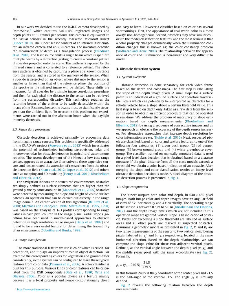
An obstacle detection decision is based on the pixel slope, itsclassification, and surrounding neighbors pixels. An obstacle isassumed to be placed on the ground, have a slope above 40� anda classification different from the green bush and red pepper cate-gories. This classification is necessary for distinguishing betweenan obstacle and a non-obstacle because the growth of bushes andfallen peppers on greenhouse paths which do not impose restric-tions on a vehicles’ ability to maneuver, are considered to benon-obstacles. Based on these characteristics, a sufficient groupof connected-component pixels (we used a threshold of 30 pixels)which are: (i) above and adjacent to the surface pixels, and (ii) clas-sified to be other than the green bush or red pepper categories,were defined as an obstacle, as seen in Fig. 4. All other cases weredefined as non-obstacles.

4. Experimental setup

We conducted the experiments in a greenhouse at the Volcanicenter, Israel. The Kinect sensor was connected to a laptop comput-er, and its data were recorded while following several greenhousepaths. The Kinect sensor was mounted on a flat surface area andthe sensor’s field of view (FOV) contains the ground and pepperbush areas. The recorded data were taken in the afternoon hourswhen the sunlight is sufficient for the Kinect’s RGB camera opera-tion and yet does not interfere with the Kinect’s depth sensoroperation. The depth sensor needs to detect the incoming infrared beams of the emitter, so the ambient light should be sig-nificantly weaker than the beams. Given these two issues, theafternoon hours provided the optimal solution, in that there wassufficient light for the RGB camera, but it was not strong enoughto interfere with the operation of the depth sensor. Our methodwas examined using records taken from four greenhouse pathsroads, termed roads 1, 2, 3, 4. The training data frames were takenfrom road 1. The test data that was used to evaluate our method,contained 158 frames from roads 2, 3 and 4. The greenhouse pathscontained 9 objects which been defined as obstacles. While travel-ing along the path obstacles appeared in consecutive frames. 87Obstacles (one or more in each frame) appear in 30 frames out ofthe 158.

4.1. Training data

The training stage, is based on manually annotated frames. Weused 12 frames from path road 1. We marked several pixel-blocksfor each color class. Every block contained a set of pixels whichrepresented the category. In the greenhouse, the predefined classesare the red pepper, green bush, brown ground and white green-house cover groups. Pixels blocks were marked for each of theclasses; for example a green bush block is presented in Fig. 5. Froma group block of pixels the class mean and covariance matrix werecalculated and stored as parameters of the color classifier. We usedseveral variants of color features, RGB, Delta-RGB((R � G) + (R � B),(G � R) + (G � B), (B � G) + (B � R)), I-RGB ((R + G+B)/3, (R � B)/2,

(a) Color classification (b) Detection based on color classifier

(c) Texture classification using LBP (d) Detection using LBP

Fig. 4. An example of an obstacle detection decision. Color map is green: bush, red: pepper, brown: ground, gray: greenhouse-cover, white: undefined: (a) color classification,(b) detection based on color classifier, (c) texture classification using LBP, (d) detection using LBP. (For interpretation of the references to color in this figure legend, the readeris referred to the web version of this article.)

Fig. 5. A green bush block mark. (For interpretation of the references to color in thisfigure legend, the reader is referred to the web version of this article.)

Table 1Mean and covariance parameters of the color classes.

Case Red pepper Green bush Brown ground White cover

R value 85.4 39.2 136.4 253.5G value 25.3 51.4 113.7 253.4B value 40.6 39.0 109.9 253.5

Pepper R G B

R 742.7 561.5 681.3G 561.5 725.9 756.3B 681.3 756.3 922.2

Bush R G B

R 643.5 699.1 724.1G 699.1 830.7 805.7B 724.1 805.7 1008

Ground R G B

R 364.1 361.9 439.2G 361.9 392.7 488.3B 439.2 488.3 659.8

Cover R G B

R 1.0 1.1 0.8G 1.1 1.5 0.9B 0.8 0.9 0.7

110 S. Nissimov et al. / Computers and Electronics in Agriculture 113 (2015) 104–115

(2G � R � B)/4), I0-RGB((R + G+B)/3, (R � B), (2G � R � B)/2) andLAB. The computed parameters of the RGB feature parametersare presented in Table 1. The LBP texture operator histograms weretrained using the same data (Fig. 6).

5. Experimental results

We applied texture features only on frames where at least oneobstacle was already detected using the color classifier. In suchcases the texture features were utilized to find more obstacles thatwere not detected based on color. A final detection decision wasmade if either color or texture classifiers were positive. This guar-anteed that the system would stay on the safe side and present all

detected obstacles and that the robotic vehicle will not bump intoan obstacle. Table 2 shows the number obstacles (out of 9) thatwere detected at least in one frame for several variants of color fea-tures. The results are shown for color and color + texture basedsystems. More detailed results of the proposed method is shownin Table 3 where we show, on a frame-level basis, the number ofdetected obstacles, miss-detected obstacles and non-obstacles thatwere detected as obstacles, out of the 87 obstacles that appear

50 100 150 200 2500

0.01

0.02

0.03

0.04

0.05

0.06S operator of green bush

(a) Green bush histogram50 100 150 200 250

0

0.01

0.02

0.03

0.04

0.05

0.06

0.07S operator of red pepper

(b) Red pepper histogram

50 100 150 200 2500

0.01

0.02

0.03

0.04

0.05

0.06S operator of brown ground

(c) Brown ground histogram50 100 150 200 250

0

0.1

0.2

0.3

0.4

0.5

0.6

0.7

0.8

0.9

1S operator of white cover

(d) White cover histogram

Fig. 6. LBP histograms for the four classes: (a) green bush histogram, (b) red pepper histogram, (c) brown ground histogram, (d) white cover histogram.

Table 2Obstacle detection results of several color features.

Color feature Obstacle detection

Color Color + texture

RGB 8/9 9/9Delta-RGB 7/9 9/9I-RGB 8/9 9/9I0-RGB 8/9 9/9Lab 8/9 9/9

S. Nissimov et al. / Computers and Electronics in Agriculture 113 (2015) 104–115 111

along the 158 test frames. Table 4 shows similar results for thesystem that is based only on color.

Fig. 7 shows an example where texture features enable detec-tion of obstacles that were not discovered primarily when onlythe color classification was used. This obstacle was not detectedinitially when we used the color classifier because its green colorcaused it to be classified as part of the green bush group. By addingthe texture classifier to our obstacle detection system we were ableto achieve 100% obstacle detection while keeping a low false posi-tive detection rate as before.

Table 3Detection performance of the proposed color + texture system. There were 87 obstacles al

Color True positive False positive

RGB 79 17Delta-RGB 67 13I-RGB 79 18I0-RGB 79 17Lab 79 17

The depth + color detection system always succeeded in detect-ing whether a frame was free of obstacles or not. In cases wherethe frame included more than one obstacle the system recognizedthe existence of obstacles but did not always successfully identifyall the obstacles. Fig. 9 show an example of frame with severalobstacles. The detected obstacle are shown by marking a contouraround the detected pixels on both the depth and the color images.This revealed in some of the cases an alignment error betweenthose images, which can be observed by comparing the contourposition of the depth (e.g. Fig. 9(b)) and the color image (e.g.Fig. 9(c)). In Fig. 9 the alignment error did not influence the detec-tion results. The obstacles were large enough so that although thealignment error occurred it did not cause a shift to another groupof pixels. Thus, part of the same pixels group was still processedand the two barrels were detected and marked with a blue contour.They were classified, as seen in Fig. 9(a), as an undefined objectcategory (colored in white pixels) and below each object thereare black pixels which represent the surface area (taken from thesuspected obstacle map). Therefore, in terms of our detection crite-ria, these objects have been identified as obstacles. Some of theleaves in the same frame, which were mistakenly identified as

ong the 158 frames of the test video sequence.

False negative Recall (%) Precision (%)

8 90.8 82.320 77.0 83.7

8 90.8 81.48 90.8 82.38 90.8 82.3

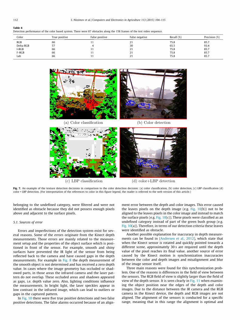
Table 4Detection performance of the color based system. There were 87 obstacles along the 158 frames of the test video sequence.

Color True positive False positive False negative Recall (%) Precision (%)

RGB 66 11 21 75.8 85.7Delta-RGB 57 4 30 65.5 93.4I-RGB 66 11 21 75.8 85.7I0-RGB 66 11 21 75.8 85.7Lab 66 11 21 75.8 85.7

(a) Color classification (b) Color detection

(c) LBP classification (d) color+LBP detection

Fig. 7. An example of the texture detection decisions in comparison to the color detection decision: (a) color classification, (b) color detection, (c) LBP classification (d)color + LBP detection. (For interpretation of the references to color in this figure legend, the reader is referred to the web version of this article.)

112 S. Nissimov et al. / Computers and Electronics in Agriculture 113 (2015) 104–115

belonging to the undefined category, were filtered and were notidentified as obstacle because they did not possess enough pixelsabove and adjacent to the surface pixels.

5.1. Sources of error

Errors and imperfections of the detection system exist for sev-eral reasons. Some of the errors originate from the Kinect depthmeasurements. Those errors are mainly related to the measure-ment setup and the properties of the object surface which is posi-tioned in front of the sensor. For example, smooth and shinysurfaces have prevented the IR light of the sensor from beingreflected back to the camera and have caused gaps in the depthmeasurements. For example in Fig. 8 the depth measurement ofthe smooth object is not determined and has received a zero depthvalue. In cases where the image geometry has occluded or shad-owed parts, in those areas the infrared camera and the laser pat-tern do not overlap. These occluded areas and shadows appearedas gaps, i.e. depth value zero. Also, lighting conditions influencethe measurements. In bright light, the laser speckles appear inlow contrast in the infrared image, which can lead to outliers orgaps in the captured pattern.

In Fig. 10 there were five true positive detections and two falsepositive detections. The false alarms occurred because of an align-

ment error between the depth and color images. This error causedthe leaves pixels on the depth image (e.g. Fig. 10(b)) not to bealigned to the leaves pixels in the color image and instead to matchthe surface pixels (e.g. Fig. 10(c)). These pixels were classified as anundefined category instead of part of the green bush group (e.g.Fig. 10(a)). Therefore, in terms of our detection criteria these leaveswere identified as obstacle.

Another possible explanation for inaccuracy in depth measure-ments can be found in (Andersen et al., 2012), which state thatwhen the Kinect sensor is rotated and quickly pointed towards adifferent scene, approximately 30 s are required until the depthvalue of the pixel reaches its final value. another source of errorcaused by the Kinect motion is synchronization inaccuraciesbetween the color and depth images and misalignment and blurof the image sensor itself.

Three main reasons were found for this synchronization prob-lem. One of the reasons is differences in the field of view betweenthe sensors. The RGB field of view is slightly larger than the field ofview of the depth sensor. It is seen clearly in Fig. 11 when examin-ing the object position near the edges of the depth and colorimages. Due to the distance between the IR camera and the RGBcamera in the Kinect device, the depth and RGB images are notaligned. The alignment of the sensors is conducted for a specificrange, meaning that in this range the alignment is optimal and

(a) Color image0

500

1000

1500

2000

2500

3000

3500

4000

4500

(b) Depth image

Fig. 8. An example of a reflective object where the sensor is not able to determine a distance to: (a) color image, (b) depth image. (For interpretation of the references to colorin this figure legend, the reader is referred to the web version of this article.)

(a) Color classification0

500

1000

1500

2000

2500

3000

3500

4000

4500

(b) Detection on depth image (c) Detection on color image

Fig. 9. An example of an obstacle detection decision based on color classification: (a) color classification, (b) detection on depth image, (c) detection on color image. (Forinterpretation of the references to color in this figure legend, the reader is referred to the web version of this article.)

(a) Classification0

500

1000

1500

2000

2500

3000

3500

4000

(b) Detection on depth image (c) Detection on color image

Fig. 10. Examples of non-obstacles that were detected as obstacles: (a) classification, (b) detection on depth image, (c) detection on color image. (For interpretation of thereferences to color in this figure legend, the reader is referred to the web version of this article.)

(a) Color image0

500

1000

1500

2000

2500

3000

3500

(b) Depth image

Fig. 11. An example of the different field of view of the sensors: (a) color image, (b) depth image. (For interpretation of the references to color in this figure legend, the readeris referred to the web version of this article.)

S. Nissimov et al. / Computers and Electronics in Agriculture 113 (2015) 104–115 113

114 S. Nissimov et al. / Computers and Electronics in Agriculture 113 (2015) 104–115

as the range of the object is increased or decreased the alignmentaccuracy decreases. Another effect that happens due to the dis-tance between the sensors is that each sensor possesses a differentview point on each of the objects which results in picturing anobject in two different angles. This effect is stronger for closerobjects. These two effects depend on the distance between the sen-sors and because this distance is short (2.5 cm) relative to the dis-tances of the objects examined, those inaccuracies are tolerable. Inaddition, problems in time synchronization between the color andthe depth sensors’ streams can cause the color and depth images tobe out of sync.

6. Conclusion

The experimental results determine that the approach present-ed can efficiently distinguish between obstacles and non-obstacles.By use of varied information such as depth, color and texture infor-mation, this method achieves satisfactory performance and its sim-ple computation enables a solution in real time. The application ofthe Kinect sensor, providing both color and depth information,enabled the development of an inexpensive obstacle detection sys-tem, using only one sensor to accomplish the task. Some alignmenterrors between the color and depth images of the Kinect sensorhave been observed. Those errors can be removed by using moreadequate calibration parameters. The texture classifier was usedin addition to the color classifier to enhance obstacle detection per-formance. The texture classifier reinforces the color classifier espe-cially in cases where the obstacles are of colors similar to one of theclassification groups. The texture classifier is capable of obstacledetection. When examining by sight its classification in compar-ison to the color classification, it is significant that the classificationsuccess rate of the texture classifier is inferior to the color classifi-er. Better texture classification can be achieved by using a higherresolution image or in this case by defining more than one patternfor some of the groups. For example, for the green bush group, theleaves that are in proximity to the camera have a very differenttexture in comparison to a group of leaves that are distant fromthe camera. Since the Kinect sensor is a contemporary develop-ment, released in November 2010, and designed for use as an Xbox360 game system controller in a household environment, littleinformation regarding the geometric quality and calibration of itsdata is available. For this purpose, it is necessary to investigatethe quality of the Kinect data in typical greenhouse conditions,which include high temperatures and increased carbon dioxideand humidity levels. Further techniques can be used in the futureto increase system performance. For example, an improved model-ing of the classification features based on ‘‘Mixture of Gaussians’’modeling can be used to improve the color classification (see e.g.Dahlkamp et al. (2006); Reina and Milella (2012)). This techniqueallows representation of the classification group for various illumi-nation conditions. For example, the color distribution under directlight and under diffuse light (shade) usually corresponds to differ-ent Gaussian modes. When using consecutive frames, the robotmotion may cause image misalignment and blur. This can beaddressed by detecting and filtering-out these frames. Anothertechnique to improve performance may be the use of a votingstrategy among multiple frames for the detection of obstacles. Thispossesses the advantage of obstacle detection that is based on anumber of frames and not on a single frame which may containpossible errors.

References

Ahonen, T., Hadid, A., Pietikainen, M., 2006. Face recognition with local binarypatterns: application to face recognition. IEEE Trans. Pattern Anal. Mach. Intell.28, 2037–2041.

Andersen, M., Jensen, T., Lisouski, P., Mortensen, A., Hansen, M., Gregersen, T.,Ahrendt, P., 2012. Kinect depth sensor evaluation for computer visionapplications. In: Technical Report ECE-TR-6, Aarhus University, Denmark.

Bellutta, P., Manduchi, R., Matthies, L., Owens, K., Rankin, A., 2000. Terrainperception for demo jjj. In: Intelligent Vehicles Conference.

Borenstein, J., Koren, Y., 1989. Real time avoidance for fast mobile robots. IEEETrans. Syst. Man Cybern. 19, 1179–1187.

Borenstein, J., Koren, Y., 1998. Obstacle avoidance with ultrasonic sensors. IEEE J.Robot. Autom. 4, 213–218.

Corke, P., Winstanley, G., Roberts, J., Duff, E., Sikka, P., 1999. Robotics for the miningindustry: opportunities and current research. In: Proceedings of theInternational Conference on Field and Service Robotics, pp. 208–219.

Dahlkamp, H., Kaehler, A., Stavens, D., Thrun, S., Bradski, G., 2006. Self-supervisedmonocular road detection in desert terrain. In: Proceedings of the RoboticsScience and Systems Conference.

Daily, M.J., Harris, J.G., Reiser, K., 1987. Detecting obstacles in range imagery. In:Image Understanding Workshop, pp. 87–97.

Discant, A., Rogozan, A., Rusu, C., Bensrhair, A., 2007. Sensors for obstacle detection– a survey. In: Electronics Technology, 30th International Spring Seminar, pp.100–105.

Foessel, A., Chheda, S., Apostolopoulos, D., 1999. Short-range millimeter wave radarperception in a polar environment. In: Proceedings of the InternationalConference on Field and Service Robotics, pp. 133–138.

Freedman, B., Shpunt, A., Machline, M., Arieli, Y., May 2010. Depth mapping usingprojected patterns. In: United States Patent Application 2010/0118123.

Guo, Z., Zhang, L., 2010. A completed modeling of local binary pattern operator fortexture classification. IEEE Trans. Image Process. 19, 1657–1663.

Harper, N., Mckerrow, P., 1999. Detecting plants for landmarks with ultrasonicsensing. In: Proceedings of the International Conference on Field and ServiceRobotics, pp. 144–149.

Henry, P., Krainin, M., Herbst, E., Ren, X., Fox, D., December 2010. RGB-D mapping:using depth cameras for dense 3D modeling of indoor environments. In:Proceedings of International Symposium on Experimental Robotics (ISER).

Huhle, B., Schairer, T., Jenke, P., Straer, W., 2010. Fusion of range and color imagesfor denoising and resolution enhancement with a non-local filter. Comput. Vis.Image Underst. 114, 1336–1345.

Khan, A., Moideen, F., Lopez, J., Khoo, W.L., Zhu, Z., 2012. Kindectect: Kinectdetecting objects. In: International Conference on Computers Helping Peoplewith Special Needs, pp. 588–595.

Khoshelham, K., Elberink, S.O., 2012. Accuracy and resolution of Kinect depth datafor indoor mapping applications. Sensors 12, 1437–1454.

Kinect, 2010. <http://www.xbox.com/en-us/kinect>.Konolige, K., 2010. Projected texture stereo. In: Proc. of the IEEE International

Conference on Robotics and Automation (ICRA).Konolige, K., Agrawal, M., Bolles, R.C., Cowan, C., Fischler, M., Gerkey, B., 2008.

Outdoor mapping and navigation using stereo vision. Exp. Robot. SpringerTracts Adv. Robot. 39, 179–190.

Krotkov, E., Fish, S., Jackel, L., McBride, B., Perschbacher, M., Pippine, J., 2007. TheDARPA perceptor evaluation experiments. In: Autonomous Robots.

Kumano, M., Ohya, A., Yuta, S., 2000. Obstacle avoidance of autonomous mobilerobot using stereo vision sensor. In: Proceedings of the 2nd InternationalSymposium on Robotics and Automation, pp. 497–502.

Langer, D., Mettenleiter, M., Hartl, F., Frohlich, C., 2000. Imaging ladar for 3Dsurveying and CAD modelling of real world environments. Int. J. Robot. Res. 19,1075–1088.

Lopez, J.J.H., Olvera, A.L.Q., Ramrez, J.L.L., Butanda, F.J.R., Manzano, M.A.I., Ojeda,D.L.A., 2012. Detecting objects using color and depth segmentation with Kinectsensor. In: The Iberoamerican Conference on Electronics Engineering andComputer Science.

Luo, R.C., Kay, M.G., 1990. A tutorial on multisensor integration and fusion. In: IEEEAnnual Conference of Industrial Electronics Society, pp. 707–722.

Ma, W., Manjunath, B., 1996. Texture features and learning similarity. In:Proceedings of the Conference on Computer Vision and Pattern Recognition(CVPR).

Manduchi, R., Castano, A., Talukder, A., Matthies, L., 2005. Obstacle detection andterrain classification for autonomous off-road navigation. Auton. Robot. 18, 81–102.

Matthies, L., Grandjean, P., 1994. Stochastic performance modeling and evaluationof obstacle detectability with imaging range sensors. IEEE Trans. Robot. Autom.10, 783–792, Special Issue on Perception-based Real World Navigation.

Matthies, L., Kelly, A., Litwin, T., Tharp, G., 1995. Obstacle detection for unmannedground vehicles: a progress report. In: Proceedings of the Intelligent VehiclesSymposium, pp. 66–71.

Matthies, L., Litwin, T., Owens, K., Rankin, A., Murphy, K., Coombs, D., Gilsinn, J.,Hong, T., Legowik, S., Nashman, M., Billibon, 1998. Performance evaluation ofUGV obstacle detection with CCD/FLIR stereo vision and LADAR. In: IEEE ISIC/CIRA/ISAS Joint Conference.

Ohanian, P., Dubes, R., 1992. Performance evaluation for four classes of texturalfeatures. Pattern Recogn. 25, 819–833.

Ohta, Y., Kanade, T., Sakai, T., 1980. Color information for region segmentation.Comput. Graph. Image Process. 13, 222–241.

Ojala, T., Pietikinen, M., Harwood, D., 1996. A comparative study of texturemeasures with classification based on featured distributions. Pattern Recogn.29, 51–59.

Ojala, T., Maenpaa, T., Pietikainen, M., Viertola, J., Kyllonen, J., Huovinen, S., 2002a.Outex-new framework for empirical evaluation of texture analysis algorithm.

S. Nissimov et al. / Computers and Electronics in Agriculture 113 (2015) 104–115 115

In: Proceedings of International Conference on Pattern Recognition, pp. 701–706.

Ojala, T., Pietikainen, M., Maenpaa, T., 2002b. Multiresolution gray-scale androtation invariant texture classification with local binary pattern. IEEE Trans.Pattern Anal. Mach. Intell. 24, 971–987.

Ortiz, J.M., Olivares, M., 2006. A vision based navigation system for an agriculturalfield robot. In: Robotics Symposium IEEE 3rd Latin American, pp. 106–114.

Palamas, G., Houzard, J.F., Kavoussanos, M., 2006. Relative position estimation of amobile robot in a greenhouse pathway. In: IEEE International Conference onIndustrial Technology.

Quigley, M., Batra, S., Gould, S., Klingbeil, E., Le, Q., Wellman, A., Ng, A.Y., 2009. High-accuracy 3D sensing for mobile manipulation: Improving object detection anddoor opening. In: IEEE International Conference on Robotics and Automation,pp. 2816–2822.

Rankin, A., Huertas, A., Matthies, L., 2005. Evaluation of stereo vision obstacledetection algorithms for off-road autonomous navigation. In: Proceedings of theAUVSI symposium on unmanned systems.

Reed, T., du Buf, J., 1993. A review of recent texture segmentation and featureextraction techniques. CVGIP: Image Process. 57, 359–372.

Reina, G., Milella, A., 2012. Towards autonomous agriculture: automatic grounddetection using trinocular stereovision. Sensors 12, 12405–12423.

Rouveure, R., Nielsen, M., Petersen, A., Reina, G., Foglia, M.M., Worst, R., Sadri, S.S.,Blas, M.R., Faure, P., Milella, A., Lykkegard, K., 2012. The QUAD-AV project:multi-sensory approach for obstacle detection in agricultural autonomousrobotics. In: International Conference of Agricultural Engineering.

Rovira-Mas, F., Zhang, Q., Reid, J.F., 2008. Stereo vision three dimensional terrainmaps for precision agriculture. Comput. Electron. Agric. 60, 133–143.

Shpunt, A., Zalevsky, Z., March 2007. Three dimensional sensing using specklepatterns. In: United States Patent Application 20090096783.

Sobottka, K., Bunke, H., 1998. Obstacle detection in range image sequences usingradial slope. In: Proc. 3rd IFAC Symposium on Intelligent Autonomous Vehicles.

Sridharan, M., Stone, P., 2009. Color learning and illumination invariance on mobilerobots: a survey. Robot. Auton. Syst. 57, 629–644.

Stentz, A., Kelly, A., Rander, P., Herman, H., Amidi, O., Mandelbaum, R., Salgian, G.,Pedersen, J., 2003. Real-time, multi-perspective perception for unmannedground vehicles. In: Proc. of AUVSI Unmanned Systems Symposium.

Viet, C., Marshall, I., 2009. An efficient obstacle detection algorithm using colour andtexture. In: World Academy of Science, Engineering and Technology.

Zhao, G., Yuta, S., 1993. Obstacle detection by vision system for an autonomousvehicle. In: Intelligent Vehicles Symposium, pp. 31–36.