Linköping University Medical DissertationsNo. 656

Computerised MicrotomographyNon-invasive imaging and analysis of biological samples, with specialreference to monitoring development of osteoporosis in small animals

Mats Stenström

Linköping 2000___________________________________________________________________________

Department of Radiation Physics, IMV, Faculty of Health Sciences,Linköping Universitet, SE-581 85 Linköping

2

ISSN 0345-0082ISBN 91-7219-757-9

Printed in Sweden by UniTryck, Linköping 2000

3

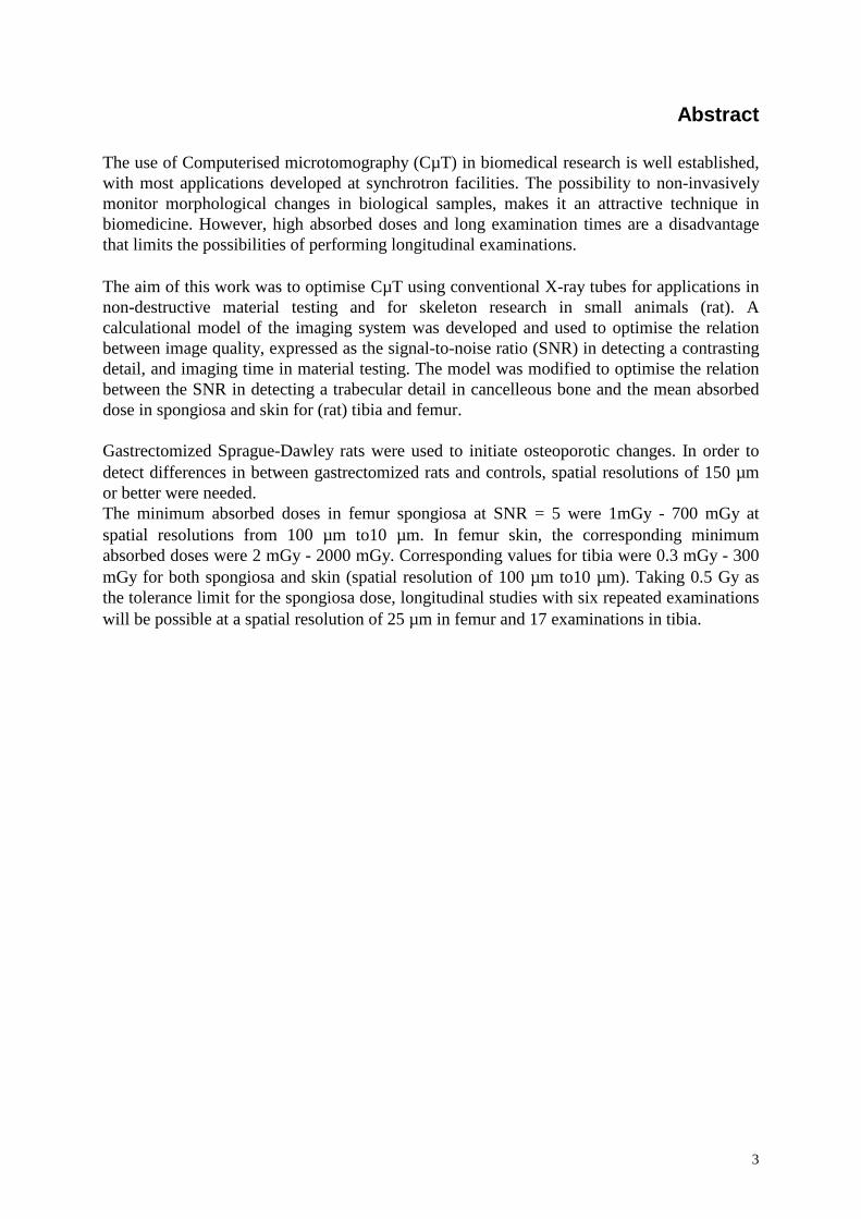
Abstract

The use of Computerised microtomography (CµT) in biomedical research is well established,with most applications developed at synchrotron facilities. The possibility to non-invasivelymonitor morphological changes in biological samples, makes it an attractive technique inbiomedicine. However, high absorbed doses and long examination times are a disadvantagethat limits the possibilities of performing longitudinal examinations.

The aim of this work was to optimise CµT using conventional X-ray tubes for applications innon-destructive material testing and for skeleton research in small animals (rat). Acalculational model of the imaging system was developed and used to optimise the relationbetween image quality, expressed as the signal-to-noise ratio (SNR) in detecting a contrastingdetail, and imaging time in material testing. The model was modified to optimise the relationbetween the SNR in detecting a trabecular detail in cancelleous bone and the mean absorbeddose in spongiosa and skin for (rat) tibia and femur.

Gastrectomized Sprague-Dawley rats were used to initiate osteoporotic changes. In order todetect differences in between gastrectomized rats and controls, spatial resolutions of 150 µmor better were needed.The minimum absorbed doses in femur spongiosa at SNR = 5 were 1mGy - 700 mGy atspatial resolutions from 100 µm to10 µm. In femur skin, the corresponding minimumabsorbed doses were 2 mGy - 2000 mGy. Corresponding values for tibia were 0.3 mGy - 300mGy for both spongiosa and skin (spatial resolution of 100 µm to10 µm). Taking 0.5 Gy asthe tolerance limit for the spongiosa dose, longitudinal studies with six repeated examinationswill be possible at a spatial resolution of 25 µm in femur and 17 examinations in tibia.

4

Content

Linköping University Medical Dissertations______________________________________ 1

Abstract ___________________________________________________________________ 3

Preface ___________________________________________________________________ 7

Introduction _______________________________________________________________ 9

Computerised tomography ___________________________________________________ 11

Data acquisition _______________________________________________________________ 11

Object Reconstruction __________________________________________________________ 12

Image quality _____________________________________________________________ 15

Image artefacts ____________________________________________________________ 17

Computerised microtomography ______________________________________________ 19

Applications of computerised microtomography _________________________________ 21

Description of the two CµT systems at Linköping University _______________________ 23

Department of Radiation Physics_________________________________________________ 23

Department of Mechanical Engineering ___________________________________________ 25

Objective of this thesis ______________________________________________________ 26

Methods__________________________________________________________________ 27

Optimisation of SNR in two different imaging tasks ________________________________ 27Optimisation in relation to imaging time _________________________________________________27Optimisation in relation to absorbed dose ________________________________________________30

Derivation of structural and mechanical characteristics ______________________________ 32Derivation of bone structural parameters from CµT images ________________________________33Measurements of bone mineral density (BMD) ____________________________________________36Mechanical testing ___________________________________________________________________36

Summary of results and discussion ____________________________________________ 37

Paper I. Methodologic aspects of CµT to monitor the development of osteoporosis ingastrectomized rats ____________________________________________________________ 37

Paper II. A theoretical model for determination of the optimal irradiation conditions forcomputerised tomography_______________________________________________________ 41

Paper III. Maximising the signal-to-noise ratio in computerised tomography data usingrobust design__________________________________________________________________ 45

Paper IV. Absorbed dose aspects in in vivo microtomography of small experimental animals_____________________________________________________________________________ 47

Longitudinal studies __________________________________________________________________48Trade off between absorbed dose and imaging time _________________________________________49

Paper V. Bone mineral density and bone structure parameters as predictors of bone strength:an analysis using CµT and gastrectomy-induced ostoepenia in the rat __________________ 51

Significance and future work ________________________________________________ 55

5

Acknowledgements _________________________________________________________ 57

References________________________________________________________________ 58

Papers _____________________________________________________________________

Paper 1. Methodologic aspects of CµT to monitor the development of osteoporosis in

gastrectomized rats ______________________________________________________________

Paper II. A theoretical model for determination of the optimal irradiation conditions for

computerised tomography_________________________________________________________

Paper III. Maximising the signal-to-noise ratio in computerised tomography data usingrobust design____________________________________________________________________

Paper IV. Absorbed dose aspects in in vivo microtomography of small experimental animals

Paper V. Bone mineral density and bone structure parameters as predictors of bone strength:an analysis using CµT and gastrectomy-induced ostoepenia in the rat ____________________

6

7

Preface

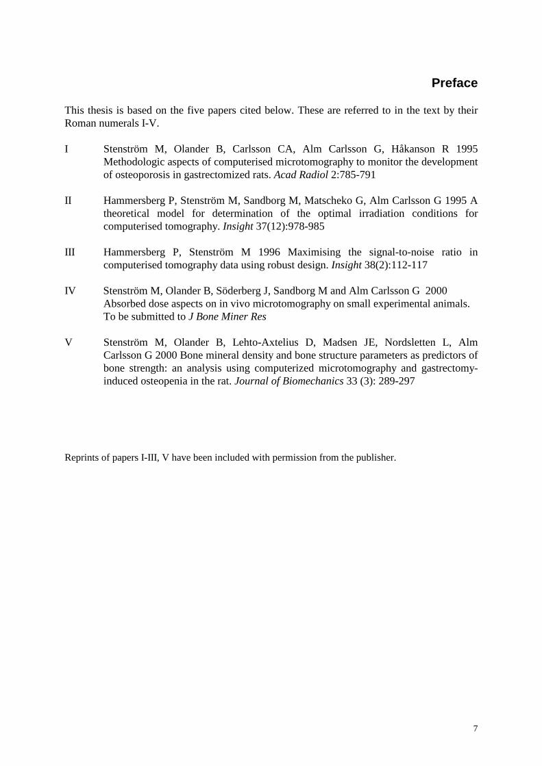
This thesis is based on the five papers cited below. These are referred to in the text by theirRoman numerals I-V.

I Stenström M, Olander B, Carlsson CA, Alm Carlsson G, Håkanson R 1995Methodologic aspects of computerised microtomography to monitor the developmentof osteoporosis in gastrectomized rats. Acad Radiol 2:785-791

II Hammersberg P, Stenström M, Sandborg M, Matscheko G, Alm Carlsson G 1995 Atheoretical model for determination of the optimal irradiation conditions forcomputerised tomography. Insight 37(12):978-985

III Hammersberg P, Stenström M 1996 Maximising the signal-to-noise ratio incomputerised tomography data using robust design. Insight 38(2):112-117

IV Stenström M, Olander B, Söderberg J, Sandborg M and Alm Carlsson G 2000Absorbed dose aspects on in vivo microtomography on small experimental animals.To be submitted to J Bone Miner Res

V Stenström M, Olander B, Lehto-Axtelius D, Madsen JE, Nordsletten L, AlmCarlsson G 2000 Bone mineral density and bone structure parameters as predictors ofbone strength: an analysis using computerized microtomography and gastrectomy-induced osteopenia in the rat. Journal of Biomechanics 33 (3): 289-297

Reprints of papers I-III, V have been included with permission from the publisher.

8

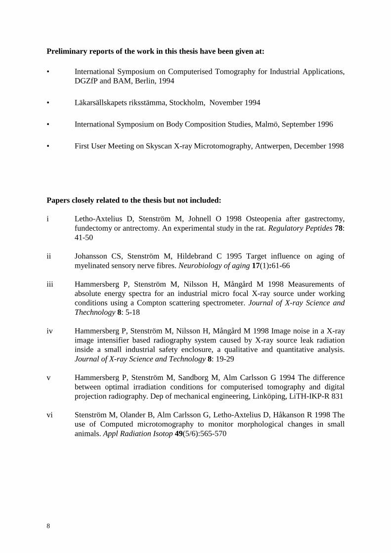
Preliminary reports of the work in this thesis have been given at:

• International Symposium on Computerised Tomography for Industrial Applications,DGZfP and BAM, Berlin, 1994

• Läkarsällskapets riksstämma, Stockholm, November 1994

• International Symposium on Body Composition Studies, Malmö, September 1996

• First User Meeting on Skyscan X-ray Microtomography, Antwerpen, December 1998

Papers closely related to the thesis but not included:

i Letho-Axtelius D, Stenström M, Johnell O 1998 Osteopenia after gastrectomy,fundectomy or antrectomy. An experimental study in the rat. Regulatory Peptides 78:41-50

ii Johansson CS, Stenström M, Hildebrand C 1995 Target influence on aging ofmyelinated sensory nerve fibres. Neurobiology of aging 17(1):61-66

iii Hammersberg P, Stenström M, Nilsson H, Mångård M 1998 Measurements ofabsolute energy spectra for an industrial micro focal X-ray source under workingconditions using a Compton scattering spectrometer. Journal of X-ray Science andThechnology 8: 5-18

iv Hammersberg P, Stenström M, Nilsson H, Mångård M 1998 Image noise in a X-rayimage intensifier based radiography system caused by X-ray source leak radiationinside a small industrial safety enclosure, a qualitative and quantitative analysis.Journal of X-ray Science and Technology 8: 19-29

v Hammersberg P, Stenström M, Sandborg M, Alm Carlsson G 1994 The differencebetween optimal irradiation conditions for computerised tomography and digitalprojection radiography. Dep of mechanical engineering, Linköping, LiTH-IKP-R 831

vi Stenström M, Olander B, Alm Carlsson G, Letho-Axtelius D, Håkanson R 1998 Theuse of Computed microtomography to monitor morphological changes in smallanimals. Appl Radiation Isotop 49(5/6):565-570

9

Introduction

The invention of Computerised Tomography (CT) by Hounsfield in the seventies was one ofthe greatest advances in diagnostic radiology. Together with Cormack, Hounsfield wasawarded the Nobel Prize in 1979. Efforts to improve CT equipment and the mathematicalreconstruction algorithms required have continued and have resulted in reduced examinationtimes and improved image quality. The spatial resolution in medical CT images today, of theorder of a few millimetres, is sufficient for most diagnostic tasks. Additional increases inspatial resolution with patients are not realistic, due to the increased absorbed doses and henceincreased radiation risk implied (Bongatz et al., 2000).

Efforts to increase spatial resolution developed in the eighties and Computerisedmicrotomography (CµT), capable of resolution of a few µm, was first reported by Sato et al1981, Elliot and Dover 1984 and Carlsson et al. 1985. Today, CµT is a well-establishedtechnique with equipment installed at many synchrotron facilities, but it is also widely usedtogether with X-ray tubes. Commercial systems with micro-focus X-ray tubes for industrial aswell as biomedical research purposes are available (Sasov and Van Dyck, 1998).

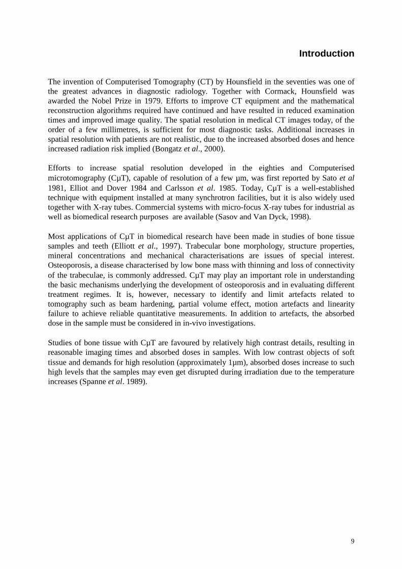
Most applications of CµT in biomedical research have been made in studies of bone tissuesamples and teeth (Elliott et al., 1997). Trabecular bone morphology, structure properties,mineral concentrations and mechanical characterisations are issues of special interest.Osteoporosis, a disease characterised by low bone mass with thinning and loss of connectivityof the trabeculae, is commonly addressed. CµT may play an important role in understandingthe basic mechanisms underlying the development of osteoporosis and in evaluating differenttreatment regimes. It is, however, necessary to identify and limit artefacts related totomography such as beam hardening, partial volume effect, motion artefacts and linearityfailure to achieve reliable quantitative measurements. In addition to artefacts, the absorbeddose in the sample must be considered in in-vivo investigations.

Studies of bone tissue with CµT are favoured by relatively high contrast details, resulting inreasonable imaging times and absorbed doses in samples. With low contrast objects of softtissue and demands for high resolution (approximately 1µm), absorbed doses increase to suchhigh levels that the samples may even get disrupted during irradiation due to the temperatureincreases (Spanne et al. 1989).

10

11

Computerised tomography

Data acquisition

In projection radiography all information along a single ray through the object is displayed asa point in a two-dimensional image. This gives in many cases sufficient information aboutinternal three-dimensional structures, if the observer has a priori knowledge of the object.Rotating the object with repeated exposures improves the information but the projectionremains a shadow image of the object. If further information is needed, we have either to cutthe object into slices or to use tomography techniques. Tomography means sliced imaging andin computerised tomography (CT), a map of the linear attenuation coefficient in the slices ofthe object is created as described below.

The basis for CT imaging relies on a statement by Radon 1917 claiming that if all projections∫= dl)y,x(fp through a point P in the plane of an object described by the object function

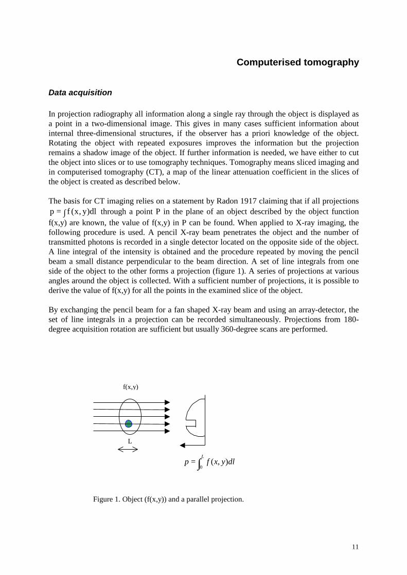
f(x,y) are known, the value of f(x,y) in P can be found. When applied to X-ray imaging, thefollowing procedure is used. A pencil X-ray beam penetrates the object and the number oftransmitted photons is recorded in a single detector located on the opposite side of the object.A line integral of the intensity is obtained and the procedure repeated by moving the pencilbeam a small distance perpendicular to the beam direction. A set of line integrals from oneside of the object to the other forms a projection (figure 1). A series of projections at variousangles around the object is collected. With a sufficient number of projections, it is possible toderive the value of f(x,y) for all the points in the examined slice of the object.

By exchanging the pencil beam for a fan shaped X-ray beam and using an array-detector, theset of line integrals in a projection can be recorded simultaneously. Projections from 180-degree acquisition rotation are sufficient but usually 360-degree scans are performed.

L

f(x,y)

∫=L

dlyxfp0

),(

Figure 1. Object (f(x,y)) and a parallel projection.

12

When the photon beam penetrates the object, the number N of photons transmitted throughthe object is, for mono-energetic photons, mathematically given by:

∫⋅=

− dllleNN

)()(

0

ρρµ

(1)

where N0 equals the number of photons incident on the object, µ/ρ is the mass attenuationcoefficient, ρ the object density and dl the path length of the photons. Without going into themathematical proof of the requirement for reconstruction from line integrals, these must belinear functions. By taking the logarithm of (1), we end up with a function that fulfils thisrequirement:

∫= dllNN )()/ln( 0 µ (2)

The use of Eq (2) to form line integrals through the object means that the object functionf(x,y) is equal to µ(x,y) where µ is the linear attenuation coefficient. The linear attenuationcoefficient is material- and energy-dependent and is the parameter that forms the image intomography.

A set of projections for all angles (θ) around the object is commonly denoted by p(r,θ) and isknown as the Radon transform of the object function f(r,θ) (Radon, 1917):

p(r,θ)= Rf(r,θ) (3)

The task of the reconstruction algorithm is to solve the problem of inversion:

f(x,y)=R-1 p(x,y) (4)

The energy dependency of f(x,y) (or the linear attenuation coefficient) is a problem when X-ray photon energy spectra are used since the requirement on linearity is then violated andgives rise to the so called beam hardening artefact. This will be discussed later.

Object Reconstruction

The art of reconstruction is purely mathematical: to solve equation (4). The methods used canbe divided into two main groups, algebraic and transform methods. The algebraicreconstruction algorithms are computationally intensive and start from a crude but intelligentguess followed by stepwise corrections until the calculated projections correspond to themeasured projections. Algebraic methods are advantageous when the signal-to-noise ratio inthe projection data is poor.

The key to accurate description of the original object function from projection data is theprojection-slice theorem (Magnusson, 1993). The theorem says: the Fourier-transform of aprojection of an object, from edge to edge, is identical with a line through the centre of the

13

two-dimensional Fourier-transform of the image. This means that, as long as all projectionsare known, the original object can be reconstructed using the inverse Fourier-transform.

The most common reconstruction algorithm is the filtered backprojection (FB). A schematicdescription of FB is given in figure 2 and a brief overview below. For details, see (Kak, 1988;Magnusson, 1993).

Each projection corresponds to a specific angel θ of the beam with respect to the object and isstored in a sinogram p(r,θ) (Edholm, 1990). A 1D Fourier-transform of each projection is thenperformed. In this step, we enter the frequency domain and the projection notation isP(R,θ). Each projection is subsequently filtered with a ramp filter according to:

Q(R,θ)=[R] x P(R,θ) (5)

By taking the inverse Fourier-transform in the R-direction, we return to the spatial domainwith filtered projections, q(r,θ). The image is finally formed by performing a back-projectionof all filtered projections.

There are a number of alternative reconstruction algorithms, such as the direct Fourier method(Magnusson, 1993) and the Linogram method (Edholm, 1990). In this work, the FB algorithmis used without exception.

Figure 2. Schematic description of the filtered back projection algorithm.

14

15

Image quality

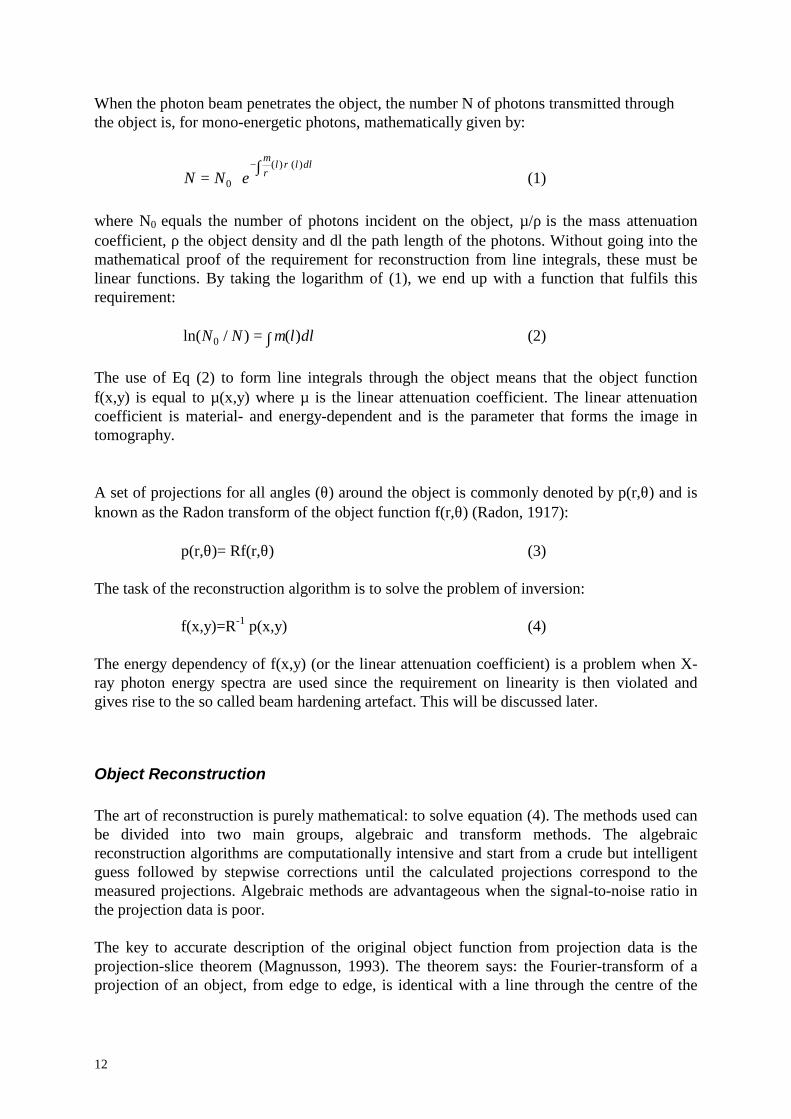
The basic physical concepts of image quality are contrast, spatial resolution and noise. Theirrelation to one another are illustrated in figure 3. The relationship between contrast and noiseis described by the signal-to-noise ratio (SNR). The modulation transfer function (MTF)describes the connection between contrast and resolution and finally, the noise powerspectrum (NPS) describes the relationship between noise and resolution. The contrast can beseparated into object contrast and image contrast (ICRU 54, 1995). Object contrast is definedas:

ρρµµ

µµµ ⋅=−= )(;

1

12C (6)

where µ1 and µ2 are the linear attenuation coefficients for the contrasting detail and thebackground, respectively and ρ the density of the object. With low energy photons,photoelectric interaction is the predominant absorption process and coherent scattering thedominant scattering process. With increased photon energy, Compton scattering becomes ofincreasing importance. Compton scattering is less dependent on material than thephotoelectric process. Thus, with increasing photon energy, the object contrast will be lesssensitive to the atomic compositions of the materials than to their density variations.

Contrast

Resolution Noise

Signal to noiseratio

Modulation transferfunction

Noise power spectrum

Imagequality

Figure 3. The relationship between the image quality parameters, contrast, resolution and noise.

16

Image contrast is the difference in grey scale (or colour) in the reconstructed image and can bemanipulated by image processing.

Noise is always present in CT images and degrades image quality. We distinguish betweenquantum noise, due to the statistics of the interaction processes in the object and the imagedetector, and electronic noise in the signal chain. Quantum noise decreases with increasingnumbers of incident photons. Cooling the detector and digitizing the signal in an early stage ofthe signal chain can reduce the electronic noise.

Spatial resolution is an equipment dependent parameter and low spatial resolution may causeimage artefacts (partial volume effects, aliasing).

17

Image artefacts

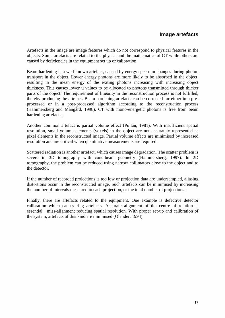
Artefacts in the image are image features which do not correspond to physical features in theobjects. Some artefacts are related to the physics and the mathematics of CT while others arecaused by deficiencies in the equipment set up or calibration.

Beam hardening is a well-known artefact, caused by energy spectrum changes during photontransport in the object. Lower energy photons are more likely to be absorbed in the object,resulting in the mean energy of the exiting photons increasing with increasing objectthickness. This causes lower µ values to be allocated to photons transmitted through thickerparts of the object. The requirement of linearity in the reconstruction process is not fulfilled,thereby producing the artefact. Beam hardening artefacts can be corrected for either in a pre-processed or in a post-processed algorithm according to the reconstruction process(Hammersberg and Mångård, 1998). CT with mono-energetic photons is free from beamhardening artefacts.

Another common artefact is partial volume effect (Pullan, 1981). With insufficient spatialresolution, small volume elements (voxels) in the object are not accurately represented aspixel elements in the reconstructed image. Partial volume effects are minimised by increasedresolution and are critical when quantitative measurements are required.

Scattered radiation is another artefact, which causes image degradation. The scatter problem issevere in 3D tomography with cone-beam geometry (Hammersberg, 1997). In 2Dtomography, the problem can be reduced using narrow collimators close to the object and tothe detector.

If the number of recorded projections is too low or projection data are undersampled, aliasingdistortions occur in the reconstructed image. Such artefacts can be minimised by increasingthe number of intervals measured in each projection, or the total number of projections.

Finally, there are artefacts related to the equipment. One example is defective detectorcalibration which causes ring artefacts. Accurate alignment of the centre of rotation isessential, miss-alignment reducing spatial resolution. With proper set-up and calibration ofthe system, artefacts of this kind are minimised (Olander, 1994).

18

19

Computerised microtomography

While computerised microtomography has been reported in the literature since the earlyeighties (Carlsson et al., 1987; Elliot and Dover, 1984; Sato, et al., 1981), there is, however,no exact definition of CµT in relation to conventional CT. Usually CµT means tomographywith spatial resolutions in the range from 100 µm down to a few µm or to even less than 1µm.

The main factor limiting the use of high spatial resolution is the limited photon fluence ratesfrom conventional X-ray sources which result in unacceptably long irradiation times andrelated problems such as focus movement (Carlsson, et al., 1987). This specific problem canbe solved by the use of synchrotron radiation sources, available in a few laboratories.Synchrotron sources have some other advantages compared to conventional X-ray tubes. Theirhigh fluence rates make it possible to use monochromators, i.e., crystals for energy tuning.This improves image quality and the possibility of achieving lower absorbed doses in theobject by appropriate optimisation.

The recent development of microfocus X-ray tubes has pushed the progress of CµT forward.Several manufactories can provide X-ray tubes with focal spot sizes less then 5 µm. Thelimited photon fluence is compensated for by a compact geometry. The small focus spotmakes possible geometrical magnification with increased spatial resolution. A further benefitof small foci is that they make promising phase contrast imaging, the latest member of thegrowing family of different tomographic modalities (Carlsson, 1999; Wilkins et al., 1996).

CµT detectors are either image intensifiers, charge couple devices (CCD) or photo diodearrays. Image intensifiers have limited spatial resolution but large detector area and highsensitivity, allowing the use of magnification techniques and cone-beam registration (Machinand Webb, 1994). CCD or photo diode arrays may be used directly or connected to intensifier-screens via light conductor. They are commonly cooled by peltier-elements in order to reducethe noise level. Pixel sizes vary from 10 µm to 50 µm and the length of the detector is usuallya few centimetres.

Common used image matrix sizes are 512x512 or 1024x1024, which might limit the spatialresolution. An object with a diameter of 10 cm corresponds to a pixel size of 10 µm whenusing a 1024x1024 matrix. Larger image matrices result in cumbersome amounts of data andlong reconstruction times.

The high spatial resolution in CµT puts high demands on the stability of the movement axisand the overall set up. To prevent image artefacts, the accuracies of all movements must bebetter than 1/10 of the resolution. This is one of the reasons why the object is rotated ratherthan the radiation source and the detector (Olander, 1994, Carlsson et al, 1987).

High spatial resolution leads to by high absorbed doses in the object, the dose increasing withthe fourth power of the resolution. This makes optimisation of the imaging chain of particularinterest in CµT. The possibility of varying X-ray tube parameters such as tube potential, anode

20

material and external filtering may be exploited to reduce absorbed doses or decrease imagingtimes.

21

Applications of computerised microtomography

Computerised microtomography with spatial resolutions from 5 µm to 50 µm has a greatpotential as a research-tool in biomedicine. In oncology, cell biology, dentistry, dermatology,orthopaedic and pharmacology, there are numbers of questions at issue where CµT might beof interest. So far, CµT investigations have been focused on bone samples, histomorphometryof bone and teeth (Elliott and Dover, 1984; Elliott et al., 1994). The structural parameters oftrabecular bone have attracted most attention for derivation of quantitative measures (Bonseet al., 1994; Cann, 1988; Durand and Rüegsegger, 1991; Feldkamp et al., 1989; Gibson, 1985;Goulet et al., 1994; Kinney et al., 1995; Stenström et al., 1995; Stenström et al., 2000).

Fracture risk is closely related to loss of bone mass but for patients with equal bone mass,there is an age-related increase in fracture risk (Kinney and Ladd, 1998). It is thus clear thatknowledge of bone mass alone is not sufficient to predict this risk. This has led investigatorsto search for aspects other than low bone mass to explain fracture occurrences. Geometricstructure, micro-damage and differences in tissue properties are often mentioned asparameters related to the mechanical properties of trabecular bone (Gibson, 1985; Goulet, etal., 1994; Kinney and Ladd, 1998). Geometric structures can be described by a number ofparameters calculated from CµT images in two or three dimensions. For improvedunderstanding of the relation between architecture and mechanical characteristics, structuralorganisation has been investigated (Kinney and Ladd, 1998). Recently, finite element methods(FEM) have been used to evaluate the parameters important with respect to bone strength andthe relation between bone structure parameters and bone mechanical properties (Keyak et al.1990; Müller and Rüegsegger, 1995). 3D cone-beam CµT has been used to generate input tothe finite element model code.

Recently longitudinal studies on rats, in which CµT was used to measure changes in the bonestructure after ovariectomy have been reported (Kinney, et al. 1995; Lane et al. 1998;Reimann et al. 1997). These studies showed promising results, but limited attention was paidto the absorbed dose in bone and the question if this might have influenced the parameter ofinterest. Earlier results from Schlegel et al.1972, Aronsson et al.1976 and Kember andCoggins, 1967 demonstrated an effect on the bone growth with absorbed doses in bone tissueless than 5 Gy. Reinmann et al. 1997 reported no effect in the rat tail at an absorbed dose of0.35 Gy. Engelke et al. 1993 recommended an absorbed dose limit of 0.5 Gy, which isconsistent with the results reported by others.

22

23

Description of the two CµT systems at Linköping University

Department of Radiation Physics

The first CµT system in Linköping was built in 1980 (Carlsson et al. 1985). New versionshave been installed during the last ten years and the system is today a flexible, totally openequipment for research purposes. Below follows a brief description of the most recent versionof the system.

A CµT acquisition system requires a radiation source, a detector unit, an object holder andmanipulators. Mounting all units on a granite table solves the requirement of mechanicalstability (figure 4). The flexible set-up offers the possibility of changing components andgeometry within extensive limits. To meet the demands of high spatial resolution combinedwith the possibility to change components, most units are step-motor controlled. Alignmentprocedures and data collection are computer controlled with resolutions of 0.1 µm (translationmovement) or rotation resolutions of 0.01 degree, respectively. To improve image quality,beam-alignment software which automatically performs alignment, has been developed(Olander, 1994). The host computer is a PC. The PC, the manipulators with the collimators,the object holder and the detector with the associated electronic units, are all mobile. Thismakes it possible to move the equipment to different radiation sources.

The X-ray tubes and detectors available are presented in Tables 1 and 2. Image reconstructionis performed with software (SNARK 87) using a filtered back-projection algorithm (Hermanand Rowland, 1978).

Manufacturer COMET COMET Siemens JEOLType MAMEX

DXmammo

78Efine focus

Bi200/20/50S

JMX-8Hmicrofocus

Tube voltages[kV]

20-49 40-110 40-150 10-50

Maximum beamcurrent [mA]

2 14 FF20 CF

3 0.1

Anod/Target material Mo W W Cr, Fe, Mo,Co, Cu, Ta

Focus size[mm]

0.1 ff0.4 cf

0.13 ff0.6 cf

1.2x1.2 0.01 pnt0.03x0.03 line

Minimum distanceFocus-object

30 mm 40 mm 40 mm 8 mm

Max load [kW] 0.6 ff4.5 cf

10 ff50 cf

50 0.2

Table 1. X-ray tubes available for tomography at the Department of Radiation Physics, Linköping (ff=fine focus, cf= coarse focus).

24

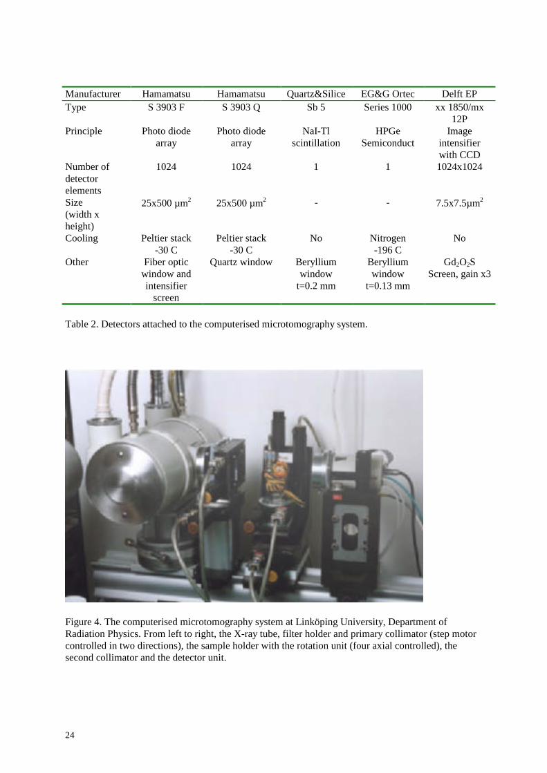
Manufacturer Hamamatsu Hamamatsu Quartz&Silice EG&G Ortec Delft EPType S 3903 F S 3903 Q Sb 5 Series 1000 xx 1850/mx

12PPrinciple Photo diode

arrayPhoto diode

arrayNaI-Tl

scintillationHPGe

SemiconductImage

intensifierwith CCD

Number ofdetectorelements

1024 1024 1 1 1024x1024

Size(width xheight)

25x500 µm2 25x500 µm2 - - 7.5x7.5µm2

Cooling Peltier stack-30 C

Peltier stack-30 C

No Nitrogen-196 C

No

Other Fiber opticwindow andintensifier

screen

Quartz window Berylliumwindow

t=0.2 mm

Berylliumwindow

t=0.13 mm

Gd2O2SScreen, gain x3

Table 2. Detectors attached to the computerised microtomography system.

Figure 4. The computerised microtomography system at Linköping University, Department ofRadiation Physics. From left to right, the X-ray tube, filter holder and primary collimator (step motorcontrolled in two directions), the sample holder with the rotation unit (four axial controlled), thesecond collimator and the detector unit.

25

Department of Mechanical Engineering

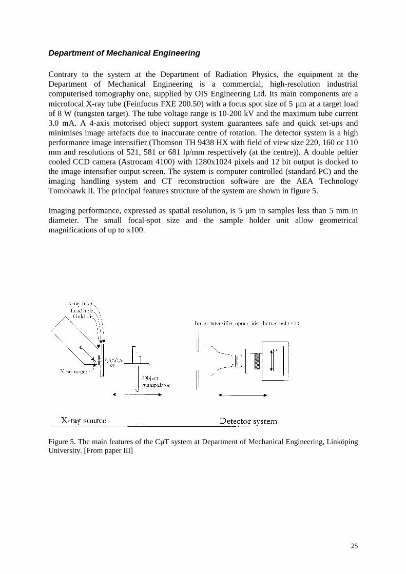
Contrary to the system at the Department of Radiation Physics, the equipment at theDepartment of Mechanical Engineering is a commercial, high-resolution industrialcomputerised tomography one, supplied by OIS Engineering Ltd. Its main components are amicrofocal X-ray tube (Feinfocus FXE 200.50) with a focus spot size of 5 µm at a target loadof 8 W (tungsten target). The tube voltage range is 10-200 kV and the maximum tube current3.0 mA. A 4-axis motorised object support system guarantees safe and quick set-ups andminimises image artefacts due to inaccurate centre of rotation. The detector system is a highperformance image intensifier (Thomson TH 9438 HX with field of view size 220, 160 or 110mm and resolutions of 521, 581 or 681 lp/mm respectively (at the centre)). A double peltiercooled CCD camera (Astrocam 4100) with 1280x1024 pixels and 12 bit output is docked tothe image intensifier output screen. The system is computer controlled (standard PC) and theimaging handling system and CT reconstruction software are the AEA TechnologyTomohawk II. The principal features structure of the system are shown in figure 5.

Imaging performance, expressed as spatial resolution, is 5 µm in samples less than 5 mm indiameter. The small focal-spot size and the sample holder unit allow geometricalmagnifications of up to x100.

Figure 5. The main features of the CµT system at Department of Mechanical Engineering, LinköpingUniversity. [From paper III]

26

Objective of this thesis

The aim of this thesis was to develop CµT methods using conventional X-ray tubes inbiomedical research and non-destructive testing in order to:

1. Optimise the relations between image quality (signal-to-noise ratio) and absorbed dose insamples or imaging time

2. Explore the use of CµT in skeleton research comprising the steps

2.1 To develop tools to quantify bone-structure parameters in the tomographic images

2.2 To optimise the conditions for performing longitudinal in vivo studies on smallanimals

27

Methods

Optimisation of SNR in two different imaging tasks

The signal-to-noise ratio (SNR) describing the relation between contrast and noise wasselected as the image quality parameter for quantifying optimisation. Being developed formonoenergetic photons and totally absorbing, photon counting detectors, previously publishedtheories on the optimisation of SNR and absorbed dose in CT systems dedicated to biomedicalresearch have several limitations (Engelke et al., 1993; Grodzins, 1983; Spanne, 1989). Inthis thesis, a realistic model has been developed in which the energy distributions of photonsfrom conventional x-ray tubes as well as the signals from partially absorbing, energyintegrating image detectors are taken into account.

Optimisation has moreover been performed for two different situations placing differentrequirements on the examination technique. First, in papers II and III, attention is focused onoptimisation of an industrial apparatus, the aim being to find the imaging technique giving thehighest SNR for a given imaging time. This gives the desired SNR at the cost of the shortestpossible examination time. In this case, focusing on non-destructive material testing, absorbeddoses are not considered to be a limiting factor.

On the other hand, when using CT techniques for imaging biomedical samples or livinganimals in longitudinal studies, absorbed dose is a most important parameter. If absorbeddoses get too high there is a risk that the biological processes being investigated will beinfluenced by radiation injury from the irradiation itself.

Optimisation in relation to imaging time

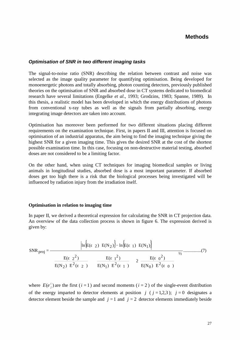
In paper II, we derived a theoretical expression for calculating the SNR in CT projection data.An overview of the data collection process is shown in figure 6. The expression derived isgiven by:

{ } { })7......(..........

½

)(E)NE(

)E(2

)(E)NE(

)E(

)(E)NE(

)E(

)NE()E(ln)NE()E(lnSNR

02

0

20

12

1

21

22

2

22

1122proj

ε⋅ε+

ε⋅ε+

ε⋅ε

⋅ε−⋅ε=

where )( ijE ε are the first ( 1=i ) and second moments ( 2=i ) of the single-event distribution

of the energy imparted to detector elements at position j ( 3,2,1=j ); 0=j designates adetector element beside the sample and 1=j and 2=j detector elements immediately beside

28

and behind the contrasting detail, respectively. )( jNE are the expectation values of thenumbers of photons incident on the corresponding detector elements.

The single-event size distribution of the energy imparted to the detector by incident primaryphotons was derived using photon transport Monte Carlo calculations. The photons wereassumed to impinge perpendicular to the surface plane of the image detector. The energyimparted to the detector by each incident primary photon (of energy 10-200 keV) wascalculated as the difference between the energy of the incident photon and the sum of allphotons escaping the detector. Photons could either interact by photoelectric absorption or bycoherent or incoherent scattering. The model is valid for large area details and does notconsider scattered radiation.

In papers II and III, the algorithm in Eq (7) was used to calculate SNRproj in projection dataas a function of tube voltage and filtration. The signal beside the object, S0, is kept constant,i.e., CENES =⋅∝ )()( 000 ε , and is chosen so that it is within the linear range of the signalresponse function (figure 7). In practice, this can be achieved by adjusting the tube current tocompensate for the variations in x-ray output at different tube voltages thereby achieving aconstant brightness on the image intensifier screen.

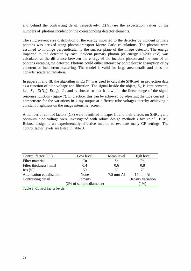
A number of control factors (CF) were identified in paper III and their effects on SNRproj andoptimum tube voltage were investigated with robust design methods (Box et al., 1978).Robust design is an experimentally effective method to evaluate many CF settings. Thecontrol factor levels are listed in table 3.

Control factor (CF) Low level Mean level High levelFilter material Cu Sn PbFilter thickness [mm] 0.4 0.6 0.8Iris [%] 50 60 70Attenuation equalisation None 7.5 mm Al 15 mm AlContrasting detail Porosity

(2% of sample diameter)Density variation

(1%)Table 3. Control factor levels

29

S0

S1

S2

detector

energy imparted

x

S1

S2

L

S0

filter

X-raysource

energy

phot

ons

Simulation model

energy

linea

r atte

nuat

ion

coef

ficie

nt, µ filter

sample

detailair

frequ

ency

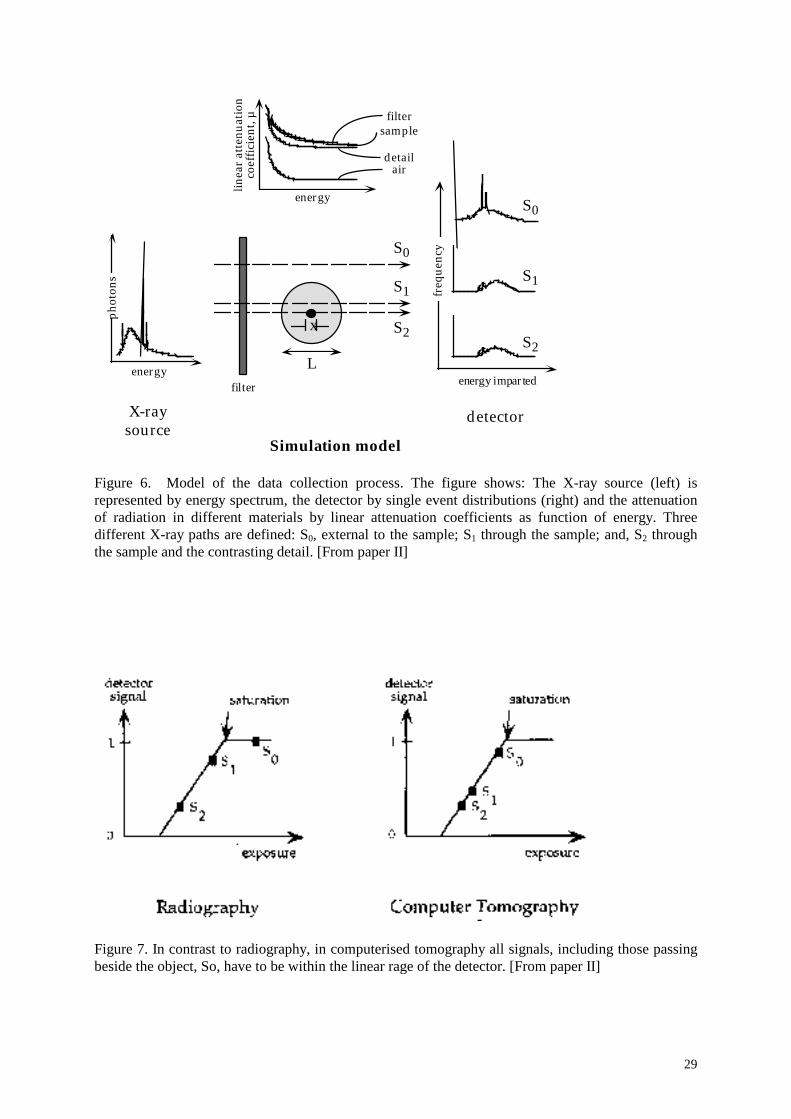
Figure 6. Model of the data collection process. The figure shows: The X-ray source (left) isrepresented by energy spectrum, the detector by single event distributions (right) and the attenuationof radiation in different materials by linear attenuation coefficients as function of energy. Threedifferent X-ray paths are defined: S0, external to the sample; S1 through the sample; and, S2 throughthe sample and the contrasting detail. [From paper II]

Figure 7. In contrast to radiography, in computerised tomography all signals, including those passingbeside the object, So, have to be within the linear rage of the detector. [From paper II]

30

Optimisation in relation to absorbed dose

In paper IV, the algorithm in Eq (7) was further elaborated to permit optimising with respectto absorbed dose in the object (biological samples). Image quality was defined as a value ofSNR=5 in the CT image and mean absorbed doses in critical tissues resulting from this imagequality requirement were derived.

Numerical methods combining bisection, secant and inverse quadratic interpolations wereused to calculate the photon fluence in the case of X-ray photon energy spectra. The meanabsorbed dose in the tissue was calculated as the product of the incident photon fluencederived from E(N0), and values of the mean absorbed dose per photon fluence calculatedusing the coupled photon-electron transport Monte Carlo code MCNP4B (Briesmeister,1993). Photons were incident on the object in a parallel beam of rectangular shape simulatinga fan-beam. The width of the beam was equal to the diameter of the sample and the beamheight 100 µm. The photon energies used were 5, 10, 15, 20, 25, 30 and 40 keV. Meanabsorbed doses per unit fluence in the skin (a soft tissue layer of thickness 100 µm) andspongiosa were calculated by dividing the energy imparted to the tissues with their masscontained in the volume irradiated by the primary photons.

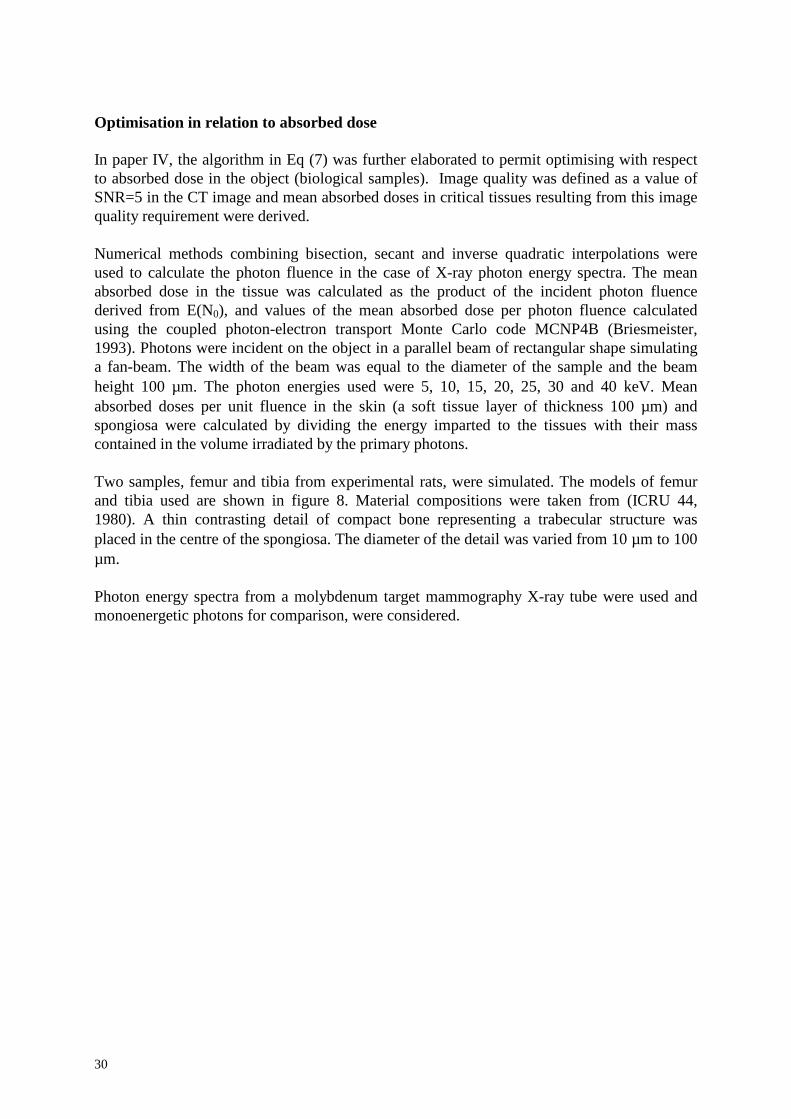
Two samples, femur and tibia from experimental rats, were simulated. The models of femurand tibia used are shown in figure 8. Material compositions were taken from (ICRU 44,1980). A thin contrasting detail of compact bone representing a trabecular structure wasplaced in the centre of the spongiosa. The diameter of the detail was varied from 10 µm to 100µm.

Photon energy spectra from a molybdenum target mammography X-ray tube were used andmonoenergetic photons for comparison, were considered.

31

12 mm

8 mm

5 mm

2 mm

4 mm6 mm

Soft tissueCortical bone

SpongiosaDetail

FemurTibia

Figure 8. Test samples with soft tissue, cortical bone and spongiosa, corresponding to the femur andtibia of rats. Femur; 12 mm in diameter with a 2 mm thick soft-tissue shell, 1.5 mm thick corticalbone shell and at the centre, a 5 mm thick spongiosa (33% cortical bone, 67% marrow,ρ = 1.18 g/cm3). Tibia; 6 mm in diameter with a 1 mm thick soft-tissue shell, 1 mm thick cortical boneshell and at the centre, a 2 mm thick spongiosa. A contrast detail of compact bone with variablediameters were placed at the centre of the spongiosa. All material specifications were taken from(ICRU 44, 1980). [From paper IV]

Measurements of the photon energy spectra

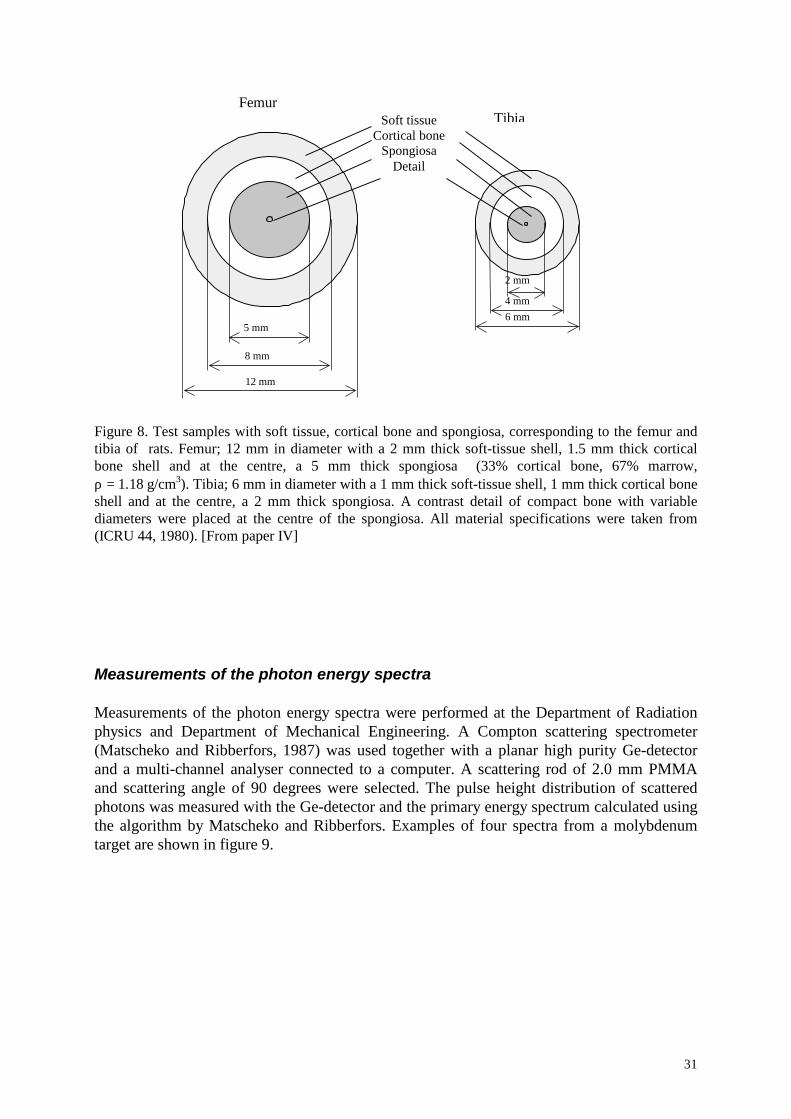
Measurements of the photon energy spectra were performed at the Department of Radiationphysics and Department of Mechanical Engineering. A Compton scattering spectrometer(Matscheko and Ribberfors, 1987) was used together with a planar high purity Ge-detectorand a multi-channel analyser connected to a computer. A scattering rod of 2.0 mm PMMAand scattering angle of 90 degrees were selected. The pulse height distribution of scatteredphotons was measured with the Ge-detector and the primary energy spectrum calculated usingthe algorithm by Matscheko and Ribberfors. Examples of four spectra from a molybdenumtarget are shown in figure 9.

32

0 5 10 15 20 25 30 35

0

0.5

1

1.5

2

2.5

3

3.5

4

4.5x 10 11

Photon energy [keV]

Photons(kev-1,mA-1,s-1,sr-1)

Figure 9. Examples of measured photon energy spectra (Mo target, 1 mm Al filtration; 26, 28, 30 and32 kV). Measurements were performed with a Compton scattering spectrometer, which explains thebroadening of the characteristic x-ray peaks at 19 and 21 keV. [From paper IV]

33

Derivation of structural and mechanical characteristics

Gastrectomy is known to cause osteopathy in experimental animals (Lehto-Axtelius et al.1998) and gastrectomized Sprague-Dawley rats were used in this study to monitor theconcomitant skeleton changes and their influence on the mechanical strength of rat bone. Theanimals were raised, treated and taken care of by our collaborators at the Department ofPharmacology, Lund University.

To answer the question of the importance of bone mineral density (BMD) relative to bonearchitecture for the mechanical strength of rat bone, measurements of BMD and mechanicaltesting were performed. The mechanical testing was performed by our collaborators at theInstitute of Surgical research, Rikshospitalet, Oslo.

Derivation of bone structural parameters from CµT images

The first step in calculating structural parameters from reconstructed CµT images is todifferentiate bone from non-bone tissue. Feldkamp et al. 1989 discuss the difficulty of relyingon a simple threshold to separate different tissues and suggested an improved method fordetermining the location of bone surfaces. In paper I, a threshold selected from an analysis ofthe linear attenuation coefficient (figure 2, paper I) was used to discriminate bone from othertissue. A more complex method was used in paper V. The tomographic image was medianfiltered using circular 5x5 pixel regions and interpolated from 5122 to 2562 pixels (figure 10a).To facilitate setting a global threshold level, beam-hardening normalisation was applied.Compact bone was for the spectrum used in this experiment normalised to a linear attenuationcoefficient value of 0.20 cm-1 (figure 10b). The trabecular region was then separated from thecortical bone with an automatic segmentation algorithm using a ”rolling ball” filter(Sternberg, 1983). Individual trabeculae were separated from bone marrow using a globalthreshold defined as (µcomp. bone + µbone marrow)/2 where µcomp.bone and µbone marrow are the linearattenuation coefficients for compact bone and bone marrow respectively. Finally a binaryimage was produced. Linear attenuation coefficients exceeding the threshold were presentedas white pixels, and those below as black (figure 10c).

34

Original image

0 1 2 3 4 5

0

1

2

3

4

5

0 20 40 60 80 100 120 140 160 180 200

0

0.05

0.1

0.15

0.2

0.25

0.3

0.35

0.4

a) b)

Trabecular and bone mask image

1.5 2 2.5 3 3.5

1

1.5

2

2.5

3

0 10 20 30 400

10

20

30Htx

0 10 20 300

10

20

30

40Hsx

0 20 40 600

10

20

30Hty

0 10 20 300

5

10

15

20

25Hsy

c) d)

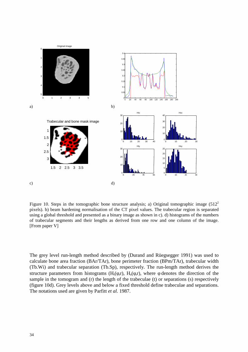
Figure 10. Steps in the tomographic bone structure analysis; a) Original tomographic image (5122

pixels). b) beam hardening normalisation of the CT pixel values. The trabecular region is separatedusing a global threshold and presented as a binary image as shown in c). d) histograms of the numbersof trabecular segments and their lengths as derived from one row and one column of the image.[From paper V]

The grey level run-length method described by (Durand and Rüegsegger 1991) was used tocalculate bone area fraction (BAr/TAr), bone perimeter fraction (BPm/TAr), trabecular width(Tb.Wi) and trabecular separation (Tb.Sp), respectively. The run-length method derives thestructure parameters from histograms (Ht(φ,r), Hs(φ,r), where φ denotes the direction of thesample in the tomogram and (r) the length of the trabeculae (t) or separations (s) respectively(figure 10d). Grey levels above and below a fixed threshold define trabeculae and separations.The notations used are given by Parfitt et al. 1987.

35

Trabecular bone area in two dimensions is equivalent to the bone volume in a threedimensional representation and according to the run-length method can be calculated from thehistogram Ht(φ,r):

pix

t

NrrH

TArBAr ∑= ),(θ

[mm2/mm2] (8)

TAr is the total area of the region of interest and BAr the total area containing bone tissue.Npix is the total number of pixels in the same region. The bone perimeter fraction is calculatedin a similar manner:

pix

t

NdrHd

TArB

2

),(22

Pr ∑××= θπ [mm/mm2] (9)

with variable d equal to the pixel area in the image. The trabecular width, given by (2 xBAr/BPr) can be written as a function of the two histograms:

∑∑×=

),(),(2

rHrrHdTrWi

t

t

θθ

π [mm] (10)

Consistently, the trabecular separation is given by

∑∑×=

),(),(2

rHrrHdTrSp

s

s

θθ

π [mm] (11)

The idea behind the run-length method is clearly seen in equations 8-11, where all fourparameters are calculated from the histograms. The model is based on the rod model oftrabecular bone tissue and is similar to other models in bone histomorphometry (Parfitt et al.,1983).

Trabecular bone architecture is extremely complex and can’t be explained exclusively by theparameters above. The number of closed loops in trabecular bone and the orientation of thenetwork are essential in determining biomechanical properties and bone strength (Goulet, etal., 1994; Kinney and Ladd, 1998). The former is called connectivity and is commonlyquantified by the Euler number (Feldkamp, et al., 1989). Kinney and Ladd investigated therelation between connectivity and trabecular bone modulus with a finite-element method.Their results indicate an important correlation between changes in connectivity and elasticstiffness. With three-dimensional data available, the Euler number is of particular interest butin isolated two-dimensional sections, it is of limited interest (Feldkamp, et al., 1989).

36

In paper I, we derived an alternative solution to the relation between architecture parametersand bone strength. The moment of inertia (J) was defined as:

dArJ ×= ∫ 2 (12)

Here, r is the distance from the area element to the axis of calculation and dA the areaelement, containing bone. The moment of inertia was used by Nordsletten et al. 1993 tocalculate the value of mechanical parameters related to bone strength.

Measurements of bone mineral density (BMD)

Bone mineral density was measured with a dual energy X-ray absorptiometry system providedwith a high resolution scanning protocol.

Mechanical testing

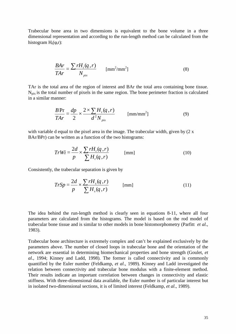
Mechanical testing was performed at the Institute for Surgical Research, Rikshospitalet Oslo.Rat femur were fractured in a hydraulic testing device (Figure 11) (Nordsletten et al., 1994).Femoral midshafts were tested by means of a three-point anterior bending and femoral necksin combined bending and compression. From the bending tests, values of ultimate bendingmoment, energy absorption to failure, bending stiffness and deflection were calculated.

Figure 11. (A) Mechanical testing of the femoral midshaft in three-point anterior bending. (B)Mechanical testing of the femoral neck in combined bending and compression.[From paper V]

37

Summary of results and discussion

Paper I. Methodologic aspects of CµT to monitor the development ofosteoporosis in gastrectomized rats

In paper I, methodological aspects of CµT in monitoring the development of osteoporosis ingastrectomized rats were considered. Spatial resolution and slice positions were tested withrespect to the possibility of discriminating between gastrectomized rats and sham operatedcontrols. Effects of gastrectomy on bone structure were quantified by the measures bonediameter, area and moment of inertia.

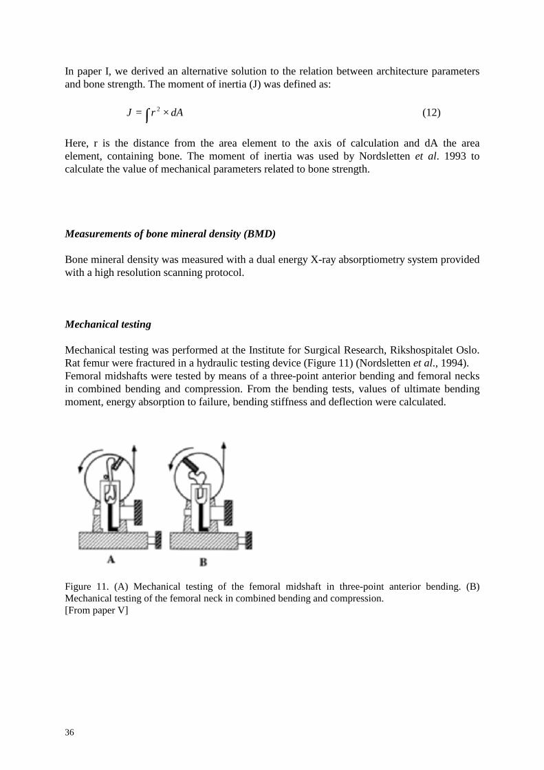
Figure 12 shows CµT images of the same slice of femur of a gastrectomized rat. Spatialresolution (pixel size) was altered from 5 µm to 500 µm in images A-F. Bone structureparameters were calculated from the images with different resolutions. Significant differencesbetween gastrectomized and control groups were established for spatial resolutions better than250 µm.

Figure 12. CµT images of the same slice of rat femur at spatial resolutions of 5 µm (A), 20 µm (B), 50µm (C), 150 µm (D), and 450 µm (E). The imaging parameters were tube potential 60 kV, 4mA,integration time/projection = 1 sec, 360 projections and slice thickness = 100 µm. In A, a microfocusX-ray tube and magnification technique were used. In F, the same specimen was imaged with aclinical CT scanner (pixel size 500 µm). [From paper I]

38

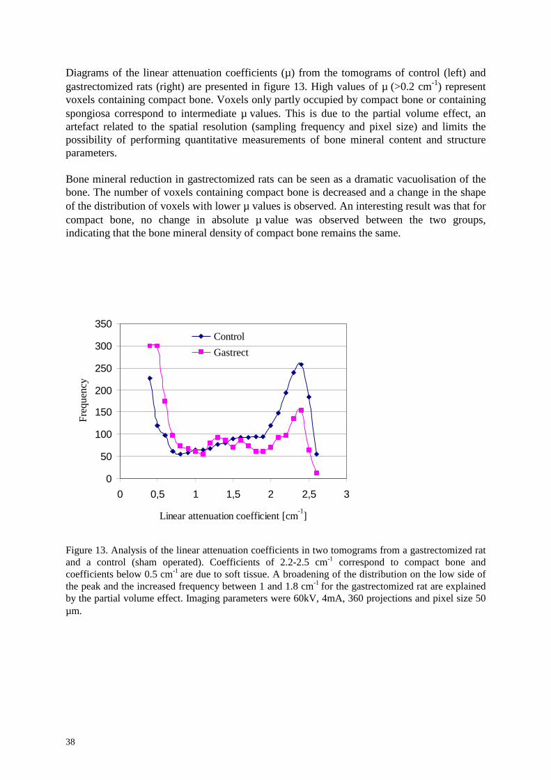
Diagrams of the linear attenuation coefficients (µ) from the tomograms of control (left) andgastrectomized rats (right) are presented in figure 13. High values of µ (>0.2 cm-1) representvoxels containing compact bone. Voxels only partly occupied by compact bone or containingspongiosa correspond to intermediate µ values. This is due to the partial volume effect, anartefact related to the spatial resolution (sampling frequency and pixel size) and limits thepossibility of performing quantitative measurements of bone mineral content and structureparameters.

Bone mineral reduction in gastrectomized rats can be seen as a dramatic vacuolisation of thebone. The number of voxels containing compact bone is decreased and a change in the shapeof the distribution of voxels with lower µ values is observed. An interesting result was that forcompact bone, no change in absolute µ value was observed between the two groups,indicating that the bone mineral density of compact bone remains the same.

0

50

100

150

200

250

300

350

0 0,5 1 1,5 2 2,5 3

Linear attenuation coefficient [cm-1]

Freq

uenc

y

ControlGastrect

Figure 13. Analysis of the linear attenuation coefficients in two tomograms from a gastrectomized ratand a control (sham operated). Coefficients of 2.2-2.5 cm-1 correspond to compact bone andcoefficients below 0.5 cm-1 are due to soft tissue. A broadening of the distribution on the low side ofthe peak and the increased frequency between 1 and 1.8 cm-1 for the gastrectomized rat are explainedby the partial volume effect. Imaging parameters were 60kV, 4mA, 360 projections and pixel size 50µm.

39

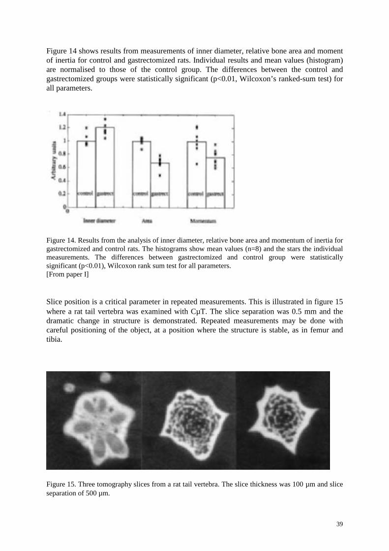
Figure 14 shows results from measurements of inner diameter, relative bone area and momentof inertia for control and gastrectomized rats. Individual results and mean values (histogram)are normalised to those of the control group. The differences between the control andgastrectomized groups were statistically significant (p<0.01, Wilcoxon’s ranked-sum test) forall parameters.

Figure 14. Results from the analysis of inner diameter, relative bone area and momentum of inertia forgastrectomized and control rats. The histograms show mean values (n=8) and the stars the individualmeasurements. The differences between gastrectomized and control group were statisticallysignificant (p<0.01), Wilcoxon rank sum test for all parameters.[From paper I]

Slice position is a critical parameter in repeated measurements. This is illustrated in figure 15where a rat tail vertebra was examined with CµT. The slice separation was 0.5 mm and thedramatic change in structure is demonstrated. Repeated measurements may be done withcareful positioning of the object, at a position where the structure is stable, as in femur andtibia.

Figure 15. Three tomography slices from a rat tail vertebra. The slice thickness was 100 µm and sliceseparation of 500 µm.

40

41

Paper II. A theoretical model for determination of the optimal irradiationconditions for computerised tomography

Figure 16 shows results from calculations and measurements on a 5.0 mm steel-cylinder witha 1.0 mm glass inclusion for tube voltages from 70 kV to 150 kV. The calculations andmeasurements show maxima at tube voltages of 100 and 105 kV respectively.

Figure 16. Comparison between simulated SNRproj for scintillator thicknesses of 300µm (— ×— ) and450µm (— •— ) and experimental measurements with a high signal and low scatter model (— — ) and95% conf. int. (— ∆— )). The sample is a 5.0mm steel cylinder with 1.0 mm glass inclusion. Thesimulation and the regression model show maxima at tube voltage of 100 and 105 kV respectively.Reconstructed images of the object at 100 kV and 140 kV are inserted. [From paper II]

42

6 0 8 0 1 0 0 1 2 0 1 4 0 1 6 00

1

2

3

4

5

6Exp . cond. 4

high s ignal , h igh scat .

6 0 8 0 1 0 0 1 2 0 1 4 0 1 6 00

1

2

3

4

5

6 Exp . cond. 1low s igna l, lo w s c a t.

SNR

proj

6 0 8 0 1 0 0 1 2 0 1 4 0 1 6 00

1

2

3

4

5

6 Exp. cond .2 h igh s ignal, lo w s c a t.

6 0 8 0 1 0 0 1 2 0 1 4 0 1 6 00

1

2

3

4

5

6E x p . cond. 3

low s igna l, high sca t .

U [ k V ]

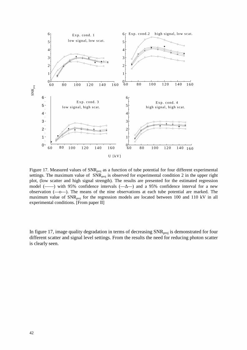
Figure 17. Measured values of SNRproj as a function of tube potential for four different experimentalsettings. The maximum value of SNRproj is observed for experimental condition 2 in the upper rightplot, (low scatter and high signal strength). The results are presented for the estimated regressionmodel (— — ) with 95% confidence intervals (— ∆— ) and a 95% confidence interval for a newobservation (— o— ). The means of the nine observations at each tube potential are marked. Themaximum value of SNRproj for the regression models are located between 100 and 110 kV in allexperimental conditions. [From paper II]

In figure 17, image quality degradation in terms of decreasing SNRproj is demonstrated for fourdifferent scatter and signal level settings. From the results the need for reducing photon scatteris clearly seen.

43

Figure 18. CµT images of a 5.0 mm steel object with 1.0 mm glass inclusion reconstructed from 256projections with high and low levels of scattered radiation for optimal and non-optimal tube voltagesrespectively a) 100 kV, high signal strength and level of scattered radiation b) 140 kV, high signalstrength and level of scattered radiation c) 100 kV, high signal strength and low level of scatteredradiation d) 140 kV, high signal strength and low level of scattered radiation. [From paper II]

In figure 18, four CµT images of the same object have been reconstructed for the differentscatter and signal settings mentioned above. The tube voltages were 100 kV and 140 kV. It isclear that even a small increase in SNR of the projections significant improves image quality,which is best in (c). Experimental conditions in (b), (140 kV, high signal, high scatter) and(d), (140kV, high signal, low scatter) illustrate the difference in image qualities expected infan beam and cone beam tomography respectively.

44

45

Paper III. Maximising the signal-to-noise ratio in computerised tomographydata using robust design

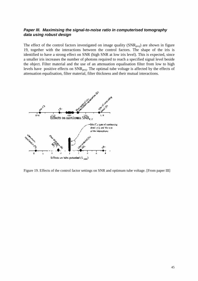
The effect of the control factors investigated on image quality (SNRproj) are shown in figure19, together with the interactions between the control factors. The shape of the iris isidentified to have a strong effect on SNR (high SNR at low iris level). This is expected, sincea smaller iris increases the number of photons required to reach a specified signal level besidethe object. Filter material and the use of an attenuation equalisation filter from low to highlevels have positive effects on SNRproj. The optimal tube voltage is affected by the effects ofattenuation equalisation, filter material, filter thickness and their mutual interactions.

Figure 19. Effects of the control factor settings on SNR and optimum tube voltage. [From paper III]

46

Figure 20.The SNRCT as a function of monoenergetic photons and for unfiltered and filtered X-rayenergy spectra (110kV); 0.8 mm copper and 0.8 mm lead filters were used. [From paper III]

In figure 20, calculated values of SNRproj for monoenergetic photons are shown (for a 5.0 mmsteel object) together with 110 kV X-ray spectra with different filters. The figure shows why alead filter is more efficient than a copper filter.

47

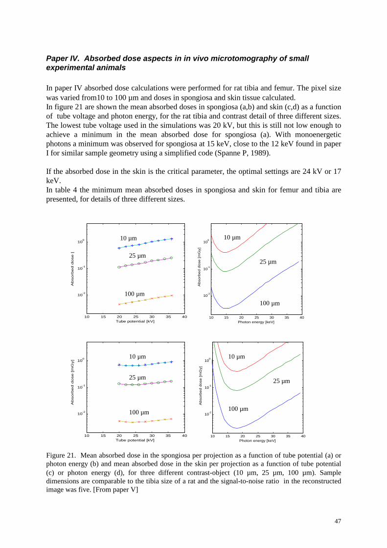
Paper IV. Absorbed dose aspects in in vivo microtomography of smallexperimental animals

In paper IV absorbed dose calculations were performed for rat tibia and femur. The pixel sizewas varied from10 to 100 µm and doses in spongiosa and skin tissue calculated.In figure 21 are shown the mean absorbed doses in spongiosa (a,b) and skin (c,d) as a functionof tube voltage and photon energy, for the rat tibia and contrast detail of three different sizes.The lowest tube voltage used in the simulations was 20 kV, but this is still not low enough toachieve a minimum in the mean absorbed dose for spongiosa (a). With monoenergeticphotons a minimum was observed for spongiosa at 15 keV, close to the 12 keV found in paperI for similar sample geometry using a simplified code (Spanne P, 1989).

If the absorbed dose in the skin is the critical parameter, the optimal settings are 24 kV or 17keV.In table 4 the minimum mean absorbed doses in spongiosa and skin for femur and tibia arepresented, for details of three different sizes.

Figure 21. Mean absorbed dose in the spongiosa per projection as a function of tube potential (a) orphoton energy (b) and mean absorbed dose in the skin per projection as a function of tube potential(c) or photon energy (d), for three different contrast-object (10 µm, 25 µm, 100 µm). Sampledimensions are comparable to the tibia size of a rat and the signal-to-noise ratio in the reconstructedimage was five. [From paper V]

10 15 20 25 30 35 40

10-2

10-1

100

Photon energy [keV]

Ab

sorb

ed

do

se [

mG

y]

10 15 20 25 30 35 40

10-2

10-1

100

Tube potential [kV]

Ab

so

rbe

d d

ose

[m

Gy]

10 15 20 25 30 35 40

10-2

10-1

100

Photon energy [keV]

Ab

sorb

ed

do

se [

mG

y]

10 15 20 25 30 35 40

10-2

10-1

100

Tube potential [kV]

Ab

so

rbe

d d

ose

[m

Gy]

10 µm

25 µm

100 µm

10 µm

25 µm

100 µm

10 µm

25 µm

100 µm

10 µm

25 µm

100 µm

48

FemurNumber ofprojections

Tube voltage[kV]

Absorbed dose[mGy]

Photon energy[keV]

Absorbed dose[mGy]

Spongiosa 10 µm 1024 20 726 15 60025 µm 512 20 69 15 59

100 µm 128 20 0.7 15 0.6 Skin 10 µm 1024 26 2034 21 1056

25 µm 512 26 192 21 99100 µm 128 26 1.9 21 0.9

TibiaNumber ofprojections

Tube voltage[kV]

Absorbed dose[mGy]

Photon energy[keV]

Absorbed dose[mGy]

Spongiosa 10 µm 512 20 302 15 21325 µm 256 20 29 15 21

100 µm 64 20 0.3 15 0.2 Skin 10 µm 512 24 336 17 214

25 µm 256 24 32 17 21100 µm 64 24 0.3 19 0.2

Table 4. Mean absorbed dose in spongiosa and skin at the optimal tube voltage or photon energy, fordifferent contrast detail sizes and numbers of projections. The signal-to-noise ratio in thereconstructed image is 5.

Longitudinal studies

In order to follow a biological sequence of events in small experimental animals, e.g., thedevelopment of osteoporosis caused by ovariectomy or gastrectomy, large groups of animalsmust be studied to avoid problems caused by biological variation within the group. Anadvantage of longitudinal studies in which the same individual is repeatedly measured is areduction in the statistical uncertainty of the measurements due to the reduced variation withinthe group. The non-invasive technique and digital format make CµT an appropriate method inlongitudinal studies.

Three factors that influence the possibility of performing repeated CµT examinations can beidentified.• The image quality (signal-to-noise ratio) required for the diagnostic task, which depends

on contrast, spatial resolution and noise.• The absorbed dose in critical organs, which need to be within acceptable limits.• The examination time which needs to be short to prevent motion artefacts and reduce

animal stress.

49

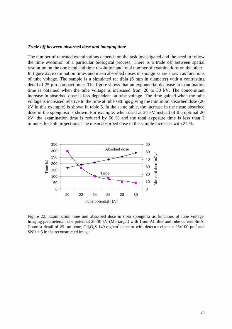
Trade off between absorbed dose and imaging time

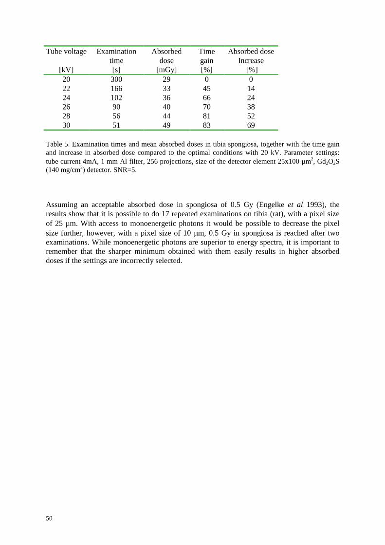
The number of repeated examinations depends on the task investigated and the need to followthe time evolution of a particular biological process. There is a trade off between spatialresolution on the one hand and time resolution and total number of examinations on the other.In figure 22, examination times and mean absorbed doses in spongiosa are shown as functionsof tube voltage. The sample is a simulated rat tibia (6 mm in diameter) with a contrastingdetail of 25 µm compact bone. The figure shows that an exponential decrease in examinationtime is obtained when the tube voltage is increased from 20 to 30 kV. The concomitantincrease in absorbed dose is less dependent on tube voltage. The time gained when the tubevoltage is increased relative to the time at tube settings giving the minimum absorbed dose (20kV in this example) is shown in table 5. In the same table, the increase in the mean absorbeddose in the spongiosa is shown. For example, when used at 24 kV instead of the optimal 20kV, the examination time is reduced by 66 % and the total exposure time is less than 2minutes for 256 projections. The mean absorbed dose in the sample increases with 24 %.

Figure 22. Examination time and absorbed dose in tibia spongiosa as functions of tube voltage.Imaging parameters: Tube potential 20-30 kV (Mo target) with 1mm Al filter and tube current 4mA.Contrast detail of 25 µm bone, Gd2O2S 140 mg/cm2 detector with detector element 25x100 µm2 andSNR = 5 in the reconstructed image.

0

50

100

150

200

250

300

350

20 22 24 26 28 30

Tube potential [kV]

Tim

e [s

]

0

10

20

30

40

50

60

Abs

orbe

d do

se [m

Gy]

Absobed dose

Time

50

Tube voltage

[kV]

Examinationtime[s]

Absorbeddose

[mGy]

Timegain[%]

Absorbed doseIncrease

[%]20 300 29 0 022 166 33 45 1424 102 36 66 2426 90 40 70 3828 56 44 81 5230 51 49 83 69

Table 5. Examination times and mean absorbed doses in tibia spongiosa, together with the time gainand increase in absorbed dose compared to the optimal conditions with 20 kV. Parameter settings:tube current 4mA, 1 mm Al filter, 256 projections, size of the detector element 25x100 µm2, Gd2O2S(140 mg/cm2) detector. SNR=5.

Assuming an acceptable absorbed dose in spongiosa of 0.5 Gy (Engelke et al 1993), theresults show that it is possible to do 17 repeated examinations on tibia (rat), with a pixel sizeof 25 µm. With access to monoenergetic photons it would be possible to decrease the pixelsize further, however, with a pixel size of 10 µm, 0.5 Gy in spongiosa is reached after twoexaminations. While monoenergetic photons are superior to energy spectra, it is important toremember that the sharper minimum obtained with them easily results in higher absorbeddoses if the settings are incorrectly selected.

51

Paper V. Bone mineral density and bone structure parameters as predictors ofbone strength: an analysis using CµT and gastrectomy-induced ostoepenia inthe rat

In paper V, the correlations between bone structure parameters, calculated from 2Dmicrotomography images, bone strength and bone mineral density were investigated. Femursfrom 21 male Sprague Dawley rats were subjected to computerised microtomographyexaminations, the three-point cantilever bending test (femoral shaft), the two-point bending-compression test (femoral neck) and dual energy absorptiometry. Modified gastrectomy wascarried out on 12 animals and 9 were sham operated.

Correlations between all result parameters were investigated as were differences between thegastrectomized and sham operated samples.

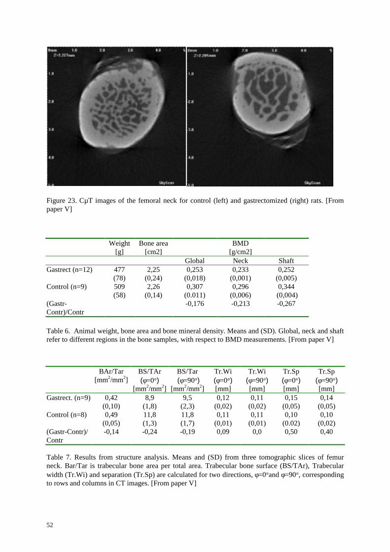
In figure 23, representative CµT images of femoral neck from gastrectomized and control ratsare shown. The number of trabecular networks is dramatically changed and large areaswithout trabeculae are seen in samples from gastrectomized rats.

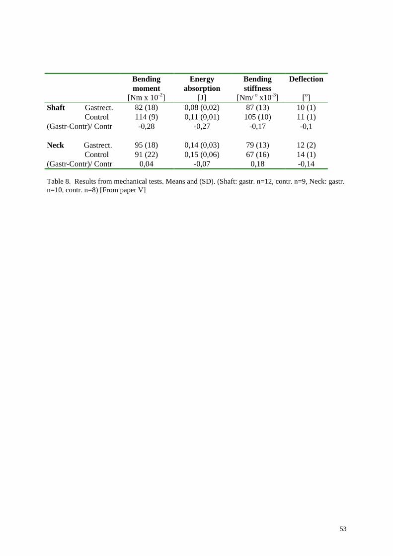
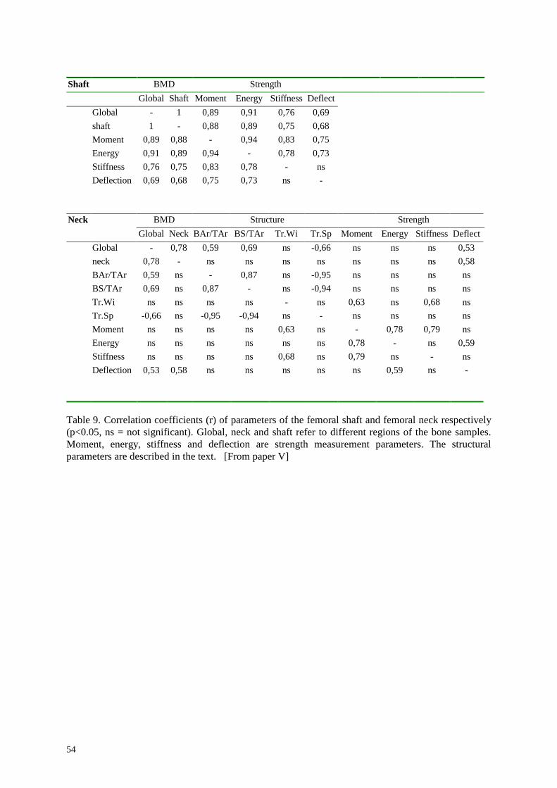
Results from measurements of BMD, structure and strength are listed in tables 6-8. Thecorrelations between measured parameters for the shaft and neck from the Pearson product-moment test are presented in table 9.

The reduction of BMD was 21% and 27% in femoral neck and shaft respectively. BMD hadan excellent correlation with all bending test parameters of the shaft. Hence, BMD is apredictor of fracture risk for non-cancellous bone. On the other hand, BMD showed nocorrelation with bone strength in the femoral neck where cancellous bone is predominant.Correlations were instead found between trabecular thickness and strength. Consequently,compared to trabecular size BMD is of limited interest in predicting fracture risk in cancellousbone.

52

Figure 23. CµT images of the femoral neck for control (left) and gastrectomized (right) rats. [Frompaper V]

Weight[g]

Bone area[cm2]

BMD[g/cm2]

Global Neck ShaftGastrect (n=12) 477

(78)2,25

(0,24)0,253

(0,018)0,233

(0,001)0,252

(0,005)Control (n=9) 509

(58)2,26

(0,14)0,307

(0.011)0,296

(0,006)0,344

(0,004)(Gastr-Contr)/Contr

-0,176 -0,213 -0,267

Table 6. Animal weight, bone area and bone mineral density. Means and (SD). Global, neck and shaftrefer to different regions in the bone samples, with respect to BMD measurements. [From paper V]

BAr/Tar[mm2/mm2]

BS/TAr(φ=0°)

[mm2/mm2]

BS/Tar (φ=9 0°)

[mm2/mm2]

Tr.Wi(φ=0°)[mm]

Tr.Wi(φ=9 0°)[mm]

Tr.Sp(φ=0°)[mm]

Tr.Sp(φ=9 0°)[mm]

Gastrect. (n=9) 0,42(0,10)

8,9(1,8)

9,5(2,3)

0,12(0,02)

0,11(0,02)

0,15(0,05)

0,14(0,05)

Control (n=8) 0,49(0,05)

11,8(1,3)

11,8(1,7)

0,11(0,01)

0,11(0,01)

0,10(0.02)

0,10(0,02)

(Gastr-Contr)/Contr

-0,14 -0,24 -0,19 0,09 0,0 0,50 0,40

Table 7. Results from structure analysis. Means and (SD) from three tomographic slices of femurneck. Bar/Tar is trabecular bone area per total area. Trabecular bone surface (BS/TAr), Trabecularwidth (Tr.Wi) and separation (Tr.Sp) are calculated for two directions, φ=0°and φ=9 0°, correspondingto rows and columns in CT images. [From paper V]

53

Bendingmoment

[Nm x 10-2]

Energyabsorption

[J]

Bendingstiffness

[Nm/ o x10-3]

Deflection

[o]Shaft Gastrect. 82 (18) 0,08 (0,02) 87 (13) 10 (1)

Control 114 (9) 0,11 (0,01) 105 (10) 11 (1)(Gastr-Contr)/ Contr -0,28 -0,27 -0,17 -0,1

Neck Gastrect. 95 (18) 0,14 (0,03) 79 (13) 12 (2) Control 91 (22) 0,15 (0,06) 67 (16) 14 (1)

(Gastr-Contr)/ Contr 0,04 -0,07 0,18 -0,14

Table 8. Results from mechanical tests. Means and (SD). (Shaft: gastr. n=12, contr. n=9, Neck: gastr.n=10, contr. n=8) [From paper V]

54

Shaft BMD StrengthGlobal Shaft Moment Energy Stiffness Deflect

Global - 1 0,89 0,91 0,76 0,69shaft 1 - 0,88 0,89 0,75 0,68Moment 0,89 0,88 - 0,94 0,83 0,75Energy 0,91 0,89 0,94 - 0,78 0,73Stiffness 0,76 0,75 0,83 0,78 - nsDeflection 0,69 0,68 0,75 0,73 ns -

Neck BMD Structure StrengthGlobal Neck BAr/TAr BS/TAr Tr.Wi Tr.Sp Moment Energy Stiffness Deflect

Global - 0,78 0,59 0,69 ns -0,66 ns ns ns 0,53neck 0,78 - ns ns ns ns ns ns ns 0,58BAr/TAr 0,59 ns - 0,87 ns -0,95 ns ns ns nsBS/TAr 0,69 ns 0,87 - ns -0,94 ns ns ns nsTr.Wi ns ns ns ns - ns 0,63 ns 0,68 nsTr.Sp -0,66 ns -0,95 -0,94 ns - ns ns ns nsMoment ns ns ns ns 0,63 ns - 0,78 0,79 nsEnergy ns ns ns ns ns ns 0,78 - ns 0,59Stiffness ns ns ns ns 0,68 ns 0,79 ns - nsDeflection 0,53 0,58 ns ns ns ns ns 0,59 ns -

Table 9. Correlation coefficients (r) of parameters of the femoral shaft and femoral neck respectively(p<0.05, ns = not significant). Global, neck and shaft refer to different regions of the bone samples.Moment, energy, stiffness and deflection are strength measurement parameters. The structuralparameters are described in the text. [From paper V]

55

Significance and future work

With the work started in paper I, a collaboration was established with the Department ofPharmacology, Lund University. They had developed an animal model with the aim toinvestigate underlying processes in bone formation and resorption, with special reference tothe pathophysiology and ethiology of osteoporosis. Their need to follow developments and toquantify effects in rats after gastrectomy was well suited to the CµT technique.Methodological aspects of the measurements with reference to image quality, spatialresolution and absorbed dose in bone tissue are discussed in paper I. The results wereunequivocal and the collaboration continued with an enquire of longitudinal studies, in vivo.The absorbed doses in spongiosa were, however, so high (5-10 Gy at 60 kV), that the boneremodulation processes, the issue of interest, could be influenced.

In paper IV, it is shown that with access to lower energy X-ray spectra and careful selection ofimaging parameters, in-vivo longitudinal studies with up to 6 repeated examinations could beperformed with spatial resolutions of ≥ 25 µm in femur and with 17 examinations in tibia.

Further development of the methodology will depend on the goals to be achieved, two of themhave been touched on in this thesis.

I. Changes in trabecular structure may, if they can be followed carefully over time, be thekey to understanding the basic mechanisms in the development of osteoporosis.Longitudinal in vivo studies are then attractive since such studies open up thepossibility of reducing the uncertainties due to biological variability betweenindividuals. However, it is likely that the needs for high spatial ( ≤5 µm) and timeresolutions will be too demanding. With increasing demand for improved spatialresolution, the sample has to be reduced in size, i.e., performed on biopsies, to fit anacceptable image matrix and to achieve reasonable imaging times and absorbed doses.

II. The practical significance of osteoporotic and other changes in bone structure is theinfluence they may have on bone strength and fracture risk. In order to study thecorrelation between bone structure and bone strength, the requirements of high spatialresolution may be reduced. Here, it may instead be more important to find the relevantmeasures of bone structure. In paper I, we introduced moment of inertia as a possiblepredictor of bone strength which should be studied further. As shown in Paper V, theissue of bone strength may not solely be one of bone architecture, since bone mineraldensity (BMD) also appears to be important. It may also be useful to be able toquantify bone mineral concentrations in different volume elements of the bone. Here,dual energy CT methods could be used but such methods are still difficult to performon an absolute scale due to image artefacts, in particular, beam hardening and partialvolume effects.

56

The study of bone micro-fracture cracks is another application where CµT techniques mightbe helpful. Micro-fracture cracks develop in bone of situations of extreme loading (Madsen etal., 1996). The healing lapse and their influence on bone strength could be investigated withCµT.

An important field within computerised tomography is how to increase knowledge of imageartefacts and their influence on the performance of quantitative measurements with CµT.Analysis of the histogram in figure 10 might be a way to correct for partial volume effects andby extension, perform quantitative measurements with comparatively low spatial resolutions.

The main world-wide focus of CµT applications has so far been on bone samples and teeth(Elliott, et al., 1997). The large object contrast and relatively small sample dimensions hasmade the method successful. However, applications to soft tissue might be the next areawhere CµT can be a helpful tool. With the totally open CµT system at the Department ofRadiation Physics, Linköping University, soft tissue applications with phase contrast CµTimaging, 2D, 3D or first generation tomography with quantitative examinations is an excitingfuture, where only limited by own imagination.

57

Acknowledgements

The present work was carried out at the Department of Radiation Physics, LinköpingUniversity. I wish to express my deep and sincere appreciation to all who have supported mein my work with this thesis.

Professor Gudrun Alm Carlsson and Professor emeritus Calle Carlsson, my two scientificsupervisors, for professional guidance and valuable criticism on all the papers. For providingexcellent working facilities and never ending enthusiasm in the project.

My close friends Birger Olander and Michael Sandborg for sharing your knowledge ofcomputers, physics and tomography. Without your help I would still be struggling with thepassword...

My good friends Peter Hammersberg and Måns Mångård for sharing the interest ofcomputerised tomography, valuable discussions and collaborations in all subjects. You haveboth significant share in this work.

The senior research staff at the Department of Radiation Physics, Eva Lund, Jan Persliden,Jojje Matcheko and Håkan Petersson for valuable discussions and advises throughout. Aspecial thanks to Eva, for always being there when I needed support.

Inger Sundgren and Ingela Allert, how so actively contributed to the familiar atmosphere atthe department.

To all friends at the Department of Radiation Physics, for sharing joy and a lot of hard work.

Stefan Ekberg, Göran Granerus and all close friends at nuclear medicine, University hospital,Linköping. For encouragement and bringing so much sun into my life.

Professor Rolf Håkansson and Daisy Axtelius, for sharing there deep knowledge inbiomedical science and fruitful collaboration.

Peter Dougan for fast and correct help in the linguistic corrections.

Finally, I would like to thank my beloved wife, Inger, for all support and her faith over theyears. For all the “funny” songs you and the kids made about me, when I was working late.

58

References

Aronson AM, Gustavsson M, and Selvik G. (1976). Acta Radiol Diagn 17, 838-844.Bongatz G, Golding S J, Leonardi M, van Meerten E v P, Geleijns J, Jessen K A, Panzer W,

Shrimpton P C, and Tosi G. (2000). European commission.Bonse U, Busch F, Gunnewig O, Beckmann F, Pahl R , Delling G, Hahn M, and Graeff W.

(1994). Bone and Mineral , 25-38.Box G, Hunter W, and Hunter S. (1978). “Statistics for experimenters.” Wiley interscience,

New York.Briesmeister J F. (1993). MCNPA A general Monte Carlo N particle transport code LA-

12625-M.Cann C E. (1988). Radiology 166, 509-522.Carlsson C, Matscheko G, and Spanne P. (1985). Med. Biol. Eng. Comput 23, 552-553.Carlsson CA. (1999). Phys. Med. Biol. 44, 23-56.Carlsson CA, Matscheko G, and Spanne P. (1987). Biol. Trace Element Res. 13, 209-217.Durand E P, and Rüegsegger P. (1991). J Comput Assist Tomogr 15, 133-139.Edholm P R. (1990). In “12th Annual international conference of the IEEE engineering in

medicine and biology society,” p. 372-373.Elliot JC, and Dover SD. (1984). Metab Bone Dis & Res 5, 219-221.Elliott JC, Anderson P, Davis G, Wong F, Dowker S E, Kozul N, and Boyde A. (1997). In

“Developments in X-ray tomography,” p. 2-12.Elliott JC, Anderson P, Gao XJ, Wong FSL, Davis GR, and Dowker SEP. (1994). J. of X-ray

science and technology 4, 102-117.Engelke K, Graeff W, Meiss L, and Delling G. (1993). Invest Radiol 23, 341-349.Feldkamp L A, Goldstein S, Parfitt M, Jesion G, and Kleerekoper M. (1989). J Bone Miner

Res 4, 3-11.Gibson L J. (1985). J. Biomechanics 18, 317-328.Goulet R W, Goldstein S A, Ciarelli M J, Kuhn J L, Brown M B, and Feldkamp L A. (1994).

J. Biomechanics 27, 375-389.Grodzins L. (1983). Nuclear Instruments and methods 206, 541-545.Hammersberg P. (1997). In “Department of Mechanical Engineering” . Linköping University,

Linköping.Hammersberg P, and Mångård M. (1998). J of x-ray science and technology 8, 75-93.Herman G, and Rowland S. (1978). . Dept of computer science, State Univ of New York,

Buffalo.ICRU 44. (1980). ICRU Publications, Washington DC.ICRU 54. (1995). ICRU Publications, Washington DC.Kak, A. C. (1988). “Principles of computerized tomographic imaging.” IEEE, PC02071.Kember NF, and Coggins J. (1967). Int J Radiat Biol 12, 143-151.Keyak J H, Meagher J M, Skinner H B, and Mote C D. (1990). J. Biomed. Eng 12, 389-397.Kinney J H, and Ladd A J. (1998). J Bone Miner Res 13, 839-845.Kinney J H, Lane N E, and Haupt D L. (1995). J Bone Mineral Res 10, 264-270.Lane N, Thompson J M, Haupt D, Kimmel D, Modin G, and Kinney J H. (1998). J Bone

Mineral Res 13, 229-236.Lehto-Axtelius D, Stenström M, and Johnell O. (1998). Reg Pept 78, 41-50.Machin K and Webb S, (1994). Phys. Med. Biol. 39, 1639-1657.

59

Madsen J E, Aune A K, Falch J A, Hukkanen M, Konttinen Y T, Santavirta S, and NordsettenL. (1996). Bone 18, 411-416.

Magnusson, M. (1993). “Dept of Electrical Engineering” . Linköping University.Matscheko G, and Ribberfors R. (1987). Phys. Med. Biol. 32, 577-594.Müller R, and Rüegsegger P. (1995). Med. Eng. Phys 17, 126-133.Nordsletten L, Kaastad TS, Skildal S, Kirkeby OJ, Reikerås O, and Ekeland A. (1993). J Bone

Miner Res 9, 1089-1095.Nordsletten L, Madsen J E, Almaas R, Roowelt T, Halse J, Konttinen Y, Hukkanen M, and

Santavirta S. (1994). Acta Orthop Scand 63, 299-304.Olander B. (1994). . Radiation Physics, Linköping University.Parfitt A, Mathews C, Villanueva A, Kleerekoper M, Frame B, and Rao D. (1983). J. clin.

Invest. 72, 1396-1409.Parfitt AM, Drezner MK, and Glorieux FH. (1987). J Bone Min Res 2, 595-610.Pullan BR. (1981). Medical Physics, Proceedings of the International School of Physics,

Enrico Fermi, Course 67 , 34-48.Radon, J. (1917). Ber. Verrh. Sächs. Akad. 69, 262.Reimann DA, Hames SM, Flynn M, and Fyhrie DP. (1997). Appl Radiat Isot 48, 1433-1436.Sasov A, and Van Dyck D. (1998). Microscopy and Analysis 3, 21-23.Sato T, Ikeda O, Yamakoshi Y, and Tsubouchi M. (1981). Appl Optics 20, 3380-3383.Schlegel D, Hilfrich J, Klemm H, and Schreckenberger H. (1972). Electromedica 1, 26-28.Spanne P. (1989). Phys. Med. Biol. 34, 679-690.Stenström M, Olander B, Carlsson CA, Alm Carlsson G, and Håkanson R. (1995). Acad

Radiol 2, 785-791.Stenström M, Olander B, Lehto-Axtelius D, Madsen J E, Nordsletten L, and Alm Carlsson G.

(2000). Journal of Biomechanics 33, 289-297.Wilkins SW, Gureyev TE, Gao D, Pogany A, and Stevenson AW. (1996). Nature 384, 335-

338.