Embed Size (px)
Citation preview
r
Computer Graphics
i
About the Tutorial
To display a picture of any size on a computer screen is a difficult process.
Computer graphics are used to simplify this process. Various algorithms and
techniques are used to generate graphics in computers. This tutorial will help you
understand how all these are processed by the computer to give a rich visual
experience to the user.
Audience
This tutorial has been prepared for students who don’t know how graphics are
used in computers. It explains the basics of graphics and how they are
implemented in computers to generate various visuals.
Prerequisites
Before you start proceeding with this tutorial, we assume that you are already
aware of the basic concepts of C programming language and basic mathematics.
Copyright & Disclaimer
Copyright 2015 by Tutorials Point (I) Pvt. Ltd.
All the content and graphics published in this e-book are the property of Tutorials
Point (I) Pvt. Ltd. The user of this e-book is prohibited to reuse, retain, copy,
distribute or republish any contents or a part of contents of this e-book in any
manner without written consent of the publisher.
We strive to update the contents of our website and tutorials as timely and as
precisely as possible, however, the contents may contain inaccuracies or errors.
Tutorials Point (I) Pvt. Ltd. provides no guarantee regarding the accuracy,
timeliness or completeness of our website or its contents including this tutorial. If
you discover any errors on our website or in this tutorial, please notify us at
Computer Graphics
ii
Table of Contents
About the Tutorial .................................................................................................................................. i
Audience ................................................................................................................................................ i
Prerequisites .......................................................................................................................................... i
Copyright & Disclaimer ........................................................................................................................... i
Table of Contents .................................................................................................................................. ii
1. COMPUTER GRAPHICS – BASICS ......................................................................................... 1
Cathode Ray Tube ................................................................................................................................. 1
Raster Scan ............................................................................................................................................ 2
Application of Computer Graphics ......................................................................................................... 3
2. LINE GENERATION ALGORITHM ......................................................................................... 5
DDA Algorithm ...................................................................................................................................... 5
Bresenham’s Line Generation ................................................................................................................ 6
Mid-Point Algorithm .............................................................................................................................. 9
3. CIRCLE GENERATION ALGORITHM ................................................................................... 11
Bresenham’s Algorithm ....................................................................................................................... 11
Mid Point Algorithm ............................................................................................................................ 13
4. POLYGON FILLING ............................................................................................................ 16
Scan Line Algorithm ............................................................................................................................. 16
Flood Fill Algorithm ............................................................................................................................. 17
Boundary Fill Algorithm ....................................................................................................................... 18
4-Connected Polygon ........................................................................................................................... 18
8-Connected Polygon ........................................................................................................................... 19
Inside-outside Test .............................................................................................................................. 21
Computer Graphics
iii
5. VIEWING AND CLIPPING ................................................................................................... 24
Point Clipping ...................................................................................................................................... 24
Line Clipping ........................................................................................................................................ 24
Cohen-Sutherland Line Clippings ......................................................................................................... 25
Cyrus-Beck Line Clipping Algorithm ..................................................................................................... 27
Polygon Clipping (Sutherland Hodgman Algorithm) ............................................................................. 28
Text Clipping ........................................................................................................................................ 29
Bitmap Graphics .................................................................................................................................. 31
6. 2D TRANSFORMATION ..................................................................................................... 33
Homogenous Coordinates ................................................................................................................... 33
Translation .......................................................................................................................................... 33
Rotation .............................................................................................................................................. 34
Scaling ................................................................................................................................................. 36
Reflection ............................................................................................................................................ 37
Shear ................................................................................................................................................... 38
Composite Transformation .................................................................................................................. 39
7. 3D GRAPHICS ................................................................................................................... 41
Parallel Projection ............................................................................................................................... 41
Orthographic Projection ...................................................................................................................... 42
Oblique Projection ............................................................................................................................... 43
Isometric Projections ........................................................................................................................... 43
Perspective Projection ......................................................................................................................... 44
Translation .......................................................................................................................................... 45
Rotation .............................................................................................................................................. 46
Scaling ................................................................................................................................................. 47
Shear ................................................................................................................................................... 48
Computer Graphics
iv
Transformation Matrices ..................................................................................................................... 49
8. CURVES ............................................................................................................................ 51
Types of Curves ................................................................................................................................... 51
Bezier Curves ....................................................................................................................................... 52
Properties of Bezier Curves .................................................................................................................. 52
B-Spline Curves .................................................................................................................................... 53
Properties of B-spline Curve ................................................................................................................ 54
9. SURFACES ........................................................................................................................ 55
Polygon Surfaces ................................................................................................................................. 55
Polygon Tables .................................................................................................................................... 55
Plane Equations ................................................................................................................................... 57
Polygon Meshes .................................................................................................................................. 57
10. VISIBLE SURFACE DETECTION ........................................................................................... 59
Depth Buffer (Z-Buffer) Method .......................................................................................................... 59
Scan-Line Method ................................................................................................................................ 61
Area-Subdivision Method .................................................................................................................... 61
Back-Face Detection ............................................................................................................................ 62
A-Buffer Method ................................................................................................................................. 64
Depth Sorting Method ......................................................................................................................... 65
Binary Space Partition (BSP) Trees ....................................................................................................... 66
11. FRACTALS ......................................................................................................................... 68
What are Fractals? ............................................................................................................................... 68
Generation of Fractals ......................................................................................................................... 68
Geometric Fractals .............................................................................................................................. 69
12. COMPUTER ANIMATION .................................................................................................. 71

Computer Graphics
v
Animation Techniques ......................................................................................................................... 71
Key Framing ......................................................................................................................................... 72
Morphing............................................................................................................................................. 73
Computer Graphics
1
Computer graphics is an art of drawing pictures on computer screens with the help of
programming. It involves computations, creation, and manipulation of data. In other
words, we can say that computer graphics is a rendering tool for the generation and
manipulation of images.
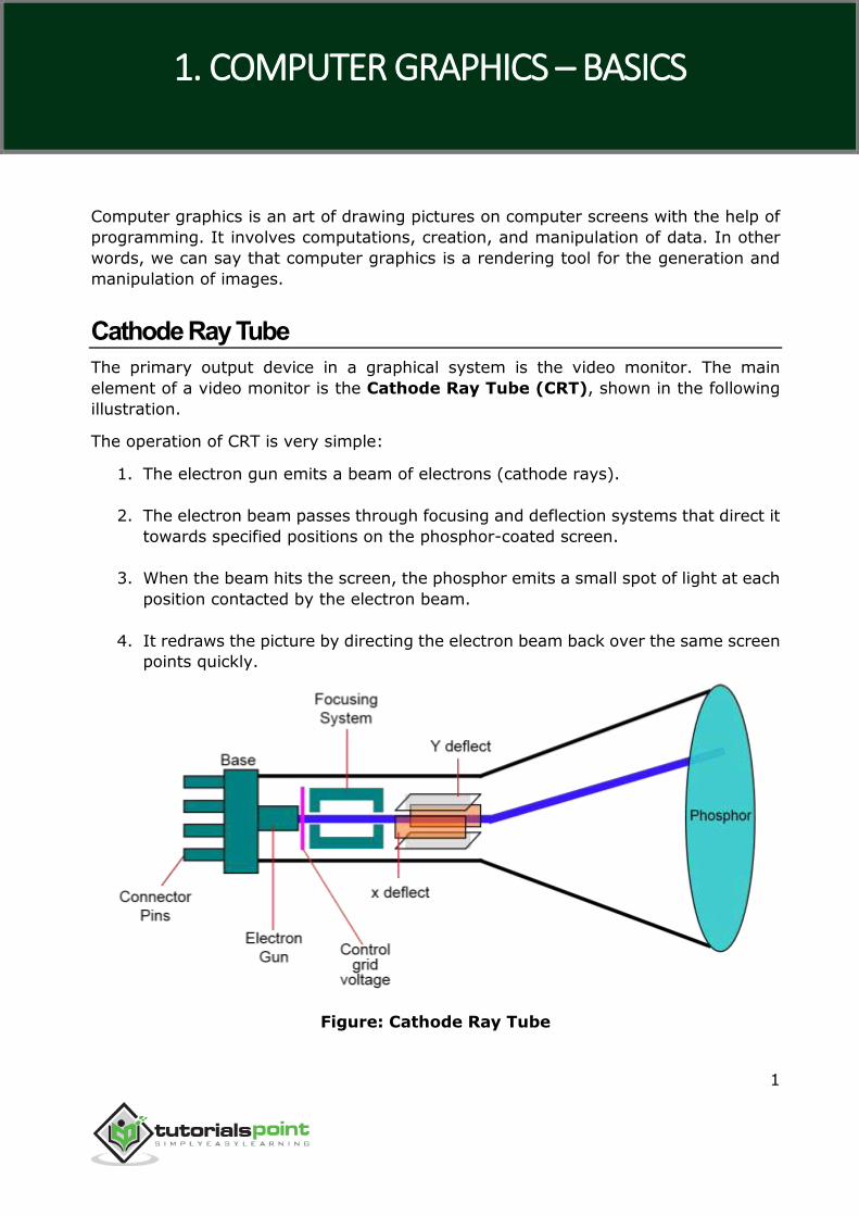
Cathode Ray Tube
The primary output device in a graphical system is the video monitor. The main
element of a video monitor is the Cathode Ray Tube (CRT), shown in the following
illustration.
The operation of CRT is very simple:
1. The electron gun emits a beam of electrons (cathode rays).
2. The electron beam passes through focusing and deflection systems that direct it
towards specified positions on the phosphor-coated screen.
3. When the beam hits the screen, the phosphor emits a small spot of light at each
position contacted by the electron beam.
4. It redraws the picture by directing the electron beam back over the same screen
points quickly.
Figure: Cathode Ray Tube
1. COMPUTER GRAPHICS – BASICS
Computer Graphics
2
There are two ways (Random scan and Raster scan) by which we can display an object
on the screen.
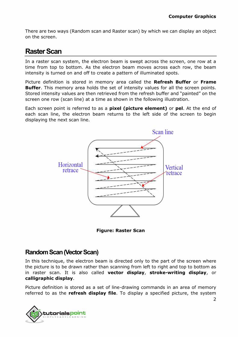
Raster Scan
In a raster scan system, the electron beam is swept across the screen, one row at a
time from top to bottom. As the electron beam moves across each row, the beam
intensity is turned on and off to create a pattern of illuminated spots.
Picture definition is stored in memory area called the Refresh Buffer or Frame
Buffer. This memory area holds the set of intensity values for all the screen points.
Stored intensity values are then retrieved from the refresh buffer and “painted” on the
screen one row (scan line) at a time as shown in the following illustration.
Each screen point is referred to as a pixel (picture element) or pel. At the end of
each scan line, the electron beam returns to the left side of the screen to begin
displaying the next scan line.
Figure: Raster Scan
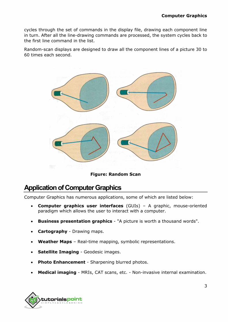
Random Scan (Vector Scan)
In this technique, the electron beam is directed only to the part of the screen where
the picture is to be drawn rather than scanning from left to right and top to bottom as
in raster scan. It is also called vector display, stroke-writing display, or
calligraphic display.
Picture definition is stored as a set of line-drawing commands in an area of memory
referred to as the refresh display file. To display a specified picture, the system
Computer Graphics
3
cycles through the set of commands in the display file, drawing each component line
in turn. After all the line-drawing commands are processed, the system cycles back to
the first line command in the list.
Random-scan displays are designed to draw all the component lines of a picture 30 to
60 times each second.
Figure: Random Scan
Application of Computer Graphics
Computer Graphics has numerous applications, some of which are listed below:
Computer graphics user interfaces (GUIs) – A graphic, mouse-oriented
paradigm which allows the user to interact with a computer.
Business presentation graphics - "A picture is worth a thousand words".
Cartography - Drawing maps.
Weather Maps – Real-time mapping, symbolic representations.
Satellite Imaging - Geodesic images.
Photo Enhancement - Sharpening blurred photos.
Medical imaging - MRIs, CAT scans, etc. - Non-invasive internal examination.
Computer Graphics
4
Engineering drawings - mechanical, electrical, civil, etc. - Replacing the blueprints of the past.
Typography - The use of character images in publishing - replacing the hard
type of the past.
Architecture - Construction plans, exterior sketches - replacing the blueprints
and hand drawings of the past.
Art - Computers provide a new medium for artists.
Training - Flight simulators, computer aided instruction, etc.
Entertainment - Movies and games.
Simulation and modeling - Replacing physical modeling and enactments
Computer Graphics
5
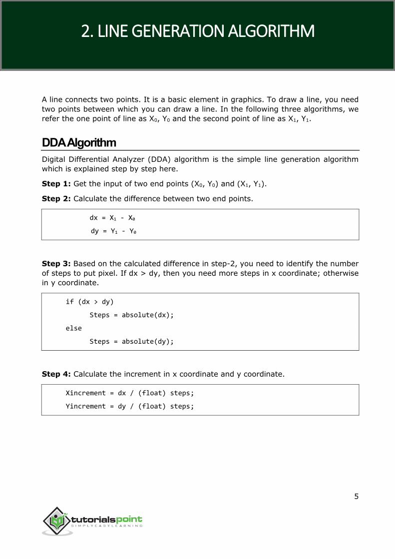
A line connects two points. It is a basic element in graphics. To draw a line, you need
two points between which you can draw a line. In the following three algorithms, we
refer the one point of line as X0, Y0 and the second point of line as X1, Y1.
DDA Algorithm
Digital Differential Analyzer (DDA) algorithm is the simple line generation algorithm
which is explained step by step here.
Step 1: Get the input of two end points (X0, Y0) and (X1, Y1).
Step 2: Calculate the difference between two end points.
dx = X1 - X0
dy = Y1 - Y0
Step 3: Based on the calculated difference in step-2, you need to identify the number
of steps to put pixel. If dx > dy, then you need more steps in x coordinate; otherwise
in y coordinate.
if (dx > dy)
Steps = absolute(dx);
else
Steps = absolute(dy);
Step 4: Calculate the increment in x coordinate and y coordinate.
Xincrement = dx / (float) steps;
Yincrement = dy / (float) steps;
2. LINE GENERATION ALGORITHM
Computer Graphics
6
Step 5: Put the pixel by successfully incrementing x and y coordinates accordingly and
complete the drawing of the line.
for(int v=0; v < Steps; v++)
{
x = x + Xincrement;
y = y + Yincrement;
putpixel(x,y);
}
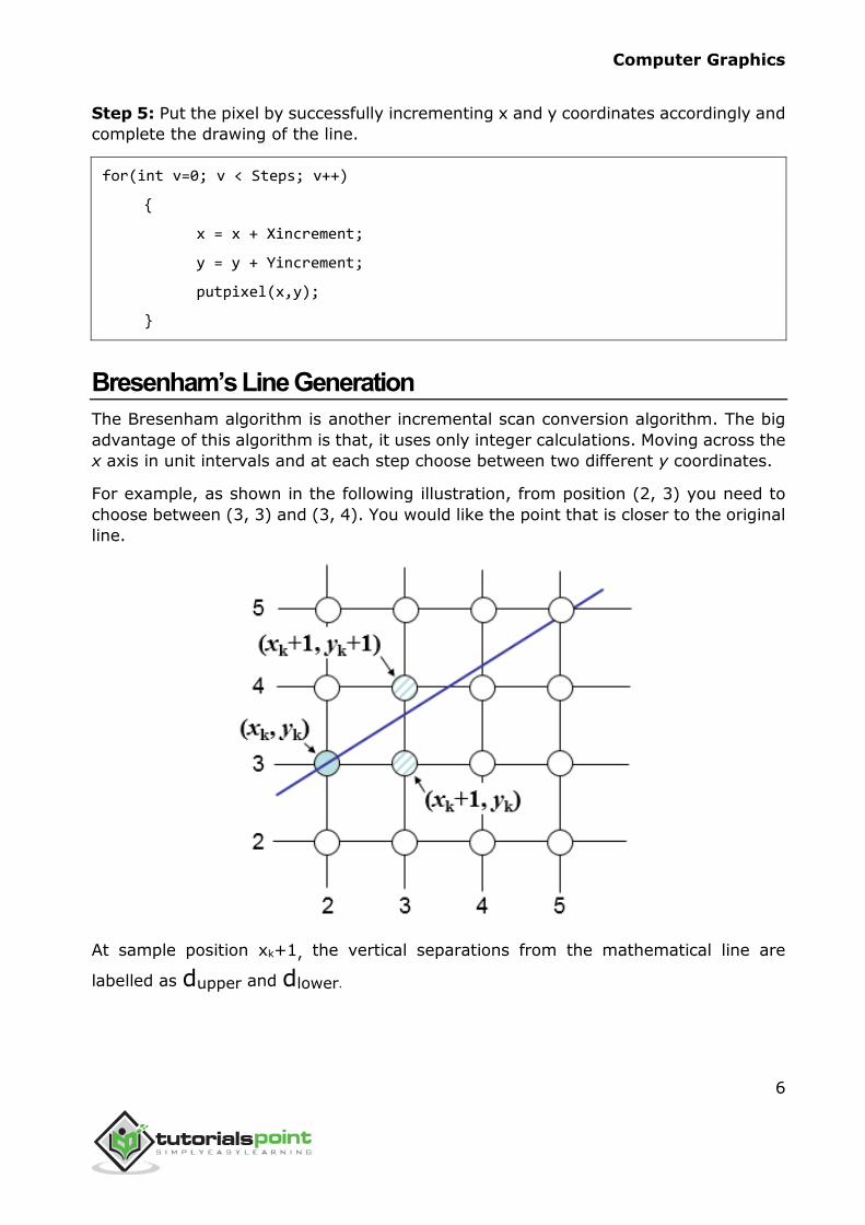
Bresenham’s Line Generation
The Bresenham algorithm is another incremental scan conversion algorithm. The big
advantage of this algorithm is that, it uses only integer calculations. Moving across the
x axis in unit intervals and at each step choose between two different y coordinates.
For example, as shown in the following illustration, from position (2, 3) you need to
choose between (3, 3) and (3, 4). You would like the point that is closer to the original
line.
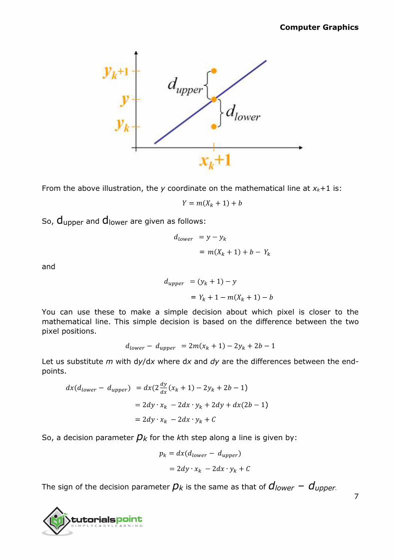
At sample position xk+1, the vertical separations from the mathematical line are
labelled as dupper and dlower.
Computer Graphics
7
From the above illustration, the y coordinate on the mathematical line at xk+1 is:
𝑌 = 𝑚(𝑋𝑘 + 1) + 𝑏
So, dupper and dlower are given as follows:
𝑑𝑙𝑜𝑤𝑒𝑟 = 𝑦 − 𝑦𝑘
= 𝑚(𝑋𝑘 + 1) + 𝑏 − 𝑌𝑘
and
𝑑𝑢𝑝𝑝𝑒𝑟 = (𝑦𝑘 + 1) − 𝑦
= 𝑌𝑘 + 1 − 𝑚(𝑋𝑘 + 1) − 𝑏
You can use these to make a simple decision about which pixel is closer to the
mathematical line. This simple decision is based on the difference between the two
pixel positions.
𝑑𝑙𝑜𝑤𝑒𝑟 − 𝑑𝑢𝑝𝑝𝑒𝑟 = 2𝑚(𝑥𝑘 + 1) − 2𝑦𝑘 + 2𝑏 − 1
Let us substitute m with dy/dx where dx and dy are the differences between the end-
points.
𝑑𝑥(𝑑𝑙𝑜𝑤𝑒𝑟 − 𝑑𝑢𝑝𝑝𝑒𝑟) = 𝑑𝑥(2𝑑𝑦
𝑑𝑥(𝑥𝑘 + 1) − 2𝑦𝑘 + 2𝑏 − 1)
= 2𝑑𝑦 ∙ 𝑥𝑘 − 2𝑑𝑥 ∙ 𝑦𝑘 + 2𝑑𝑦 + 𝑑𝑥(2𝑏 − 1)
= 2𝑑𝑦 ∙ 𝑥𝑘 − 2𝑑𝑥 ∙ 𝑦𝑘 + 𝐶
So, a decision parameter pk for the kth step along a line is given by:
𝑝𝑘 = 𝑑𝑥(𝑑𝑙𝑜𝑤𝑒𝑟 − 𝑑𝑢𝑝𝑝𝑒𝑟)
= 2𝑑𝑦 ∙ 𝑥𝑘 − 2𝑑𝑥 ∙ 𝑦𝑘 + 𝐶
The sign of the decision parameter pk is the same as that of dlower – dupper.
Computer Graphics
8
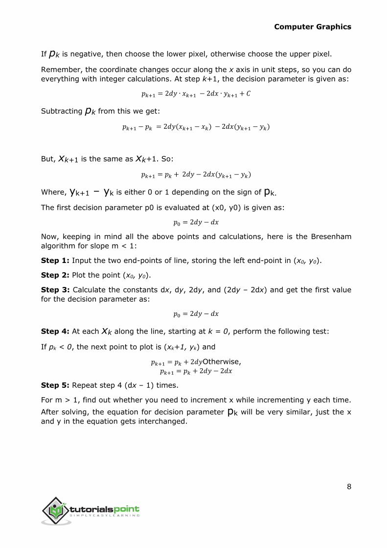
If pk is negative, then choose the lower pixel, otherwise choose the upper pixel.
Remember, the coordinate changes occur along the x axis in unit steps, so you can do
everything with integer calculations. At step k+1, the decision parameter is given as:
𝑝𝑘+1 = 2𝑑𝑦 ∙ 𝑥𝑘+1 − 2𝑑𝑥 ∙ 𝑦𝑘+1 + 𝐶
Subtracting pk from this we get:
𝑝𝑘+1 − 𝑝𝑘 = 2𝑑𝑦(𝑥𝑘+1 − 𝑥𝑘) − 2𝑑𝑥(𝑦𝑘+1 − 𝑦𝑘)
But, xk+1 is the same as xk+1. So:
𝑝𝑘+1 = 𝑝𝑘 + 2𝑑𝑦 − 2𝑑𝑥(𝑦𝑘+1 − 𝑦𝑘)
Where, yk+1 – yk is either 0 or 1 depending on the sign of pk.
The first decision parameter p0 is evaluated at (x0, y0) is given as:
𝑝0 = 2𝑑𝑦 − 𝑑𝑥
Now, keeping in mind all the above points and calculations, here is the Bresenham
algorithm for slope m < 1:
Step 1: Input the two end-points of line, storing the left end-point in (x0, y0).
Step 2: Plot the point (x0, y0).
Step 3: Calculate the constants dx, dy, 2dy, and (2dy – 2dx) and get the first value
for the decision parameter as:
𝑝0 = 2𝑑𝑦 − 𝑑𝑥
Step 4: At each xk along the line, starting at k = 0, perform the following test:
If pk < 0, the next point to plot is (xk+1, yk) and
𝑝𝑘+1 = 𝑝𝑘 + 2𝑑𝑦Otherwise,
𝑝𝑘+1 = 𝑝𝑘 + 2𝑑𝑦 − 2𝑑𝑥
Step 5: Repeat step 4 (dx – 1) times.
For m > 1, find out whether you need to increment x while incrementing y each time.
After solving, the equation for decision parameter pk will be very similar, just the x
and y in the equation gets interchanged.
Computer Graphics
9
Mid-Point Algorithm
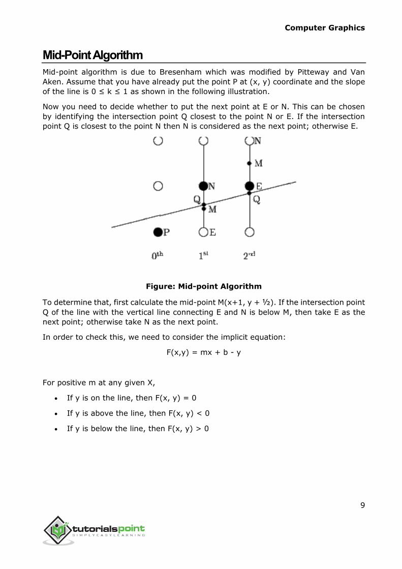
Mid-point algorithm is due to Bresenham which was modified by Pitteway and Van
Aken. Assume that you have already put the point P at (x, y) coordinate and the slope
of the line is 0 ≤ k ≤ 1 as shown in the following illustration.
Now you need to decide whether to put the next point at E or N. This can be chosen
by identifying the intersection point Q closest to the point N or E. If the intersection
point Q is closest to the point N then N is considered as the next point; otherwise E.
Figure: Mid-point Algorithm
To determine that, first calculate the mid-point M(x+1, y + ½). If the intersection point
Q of the line with the vertical line connecting E and N is below M, then take E as the
next point; otherwise take N as the next point.
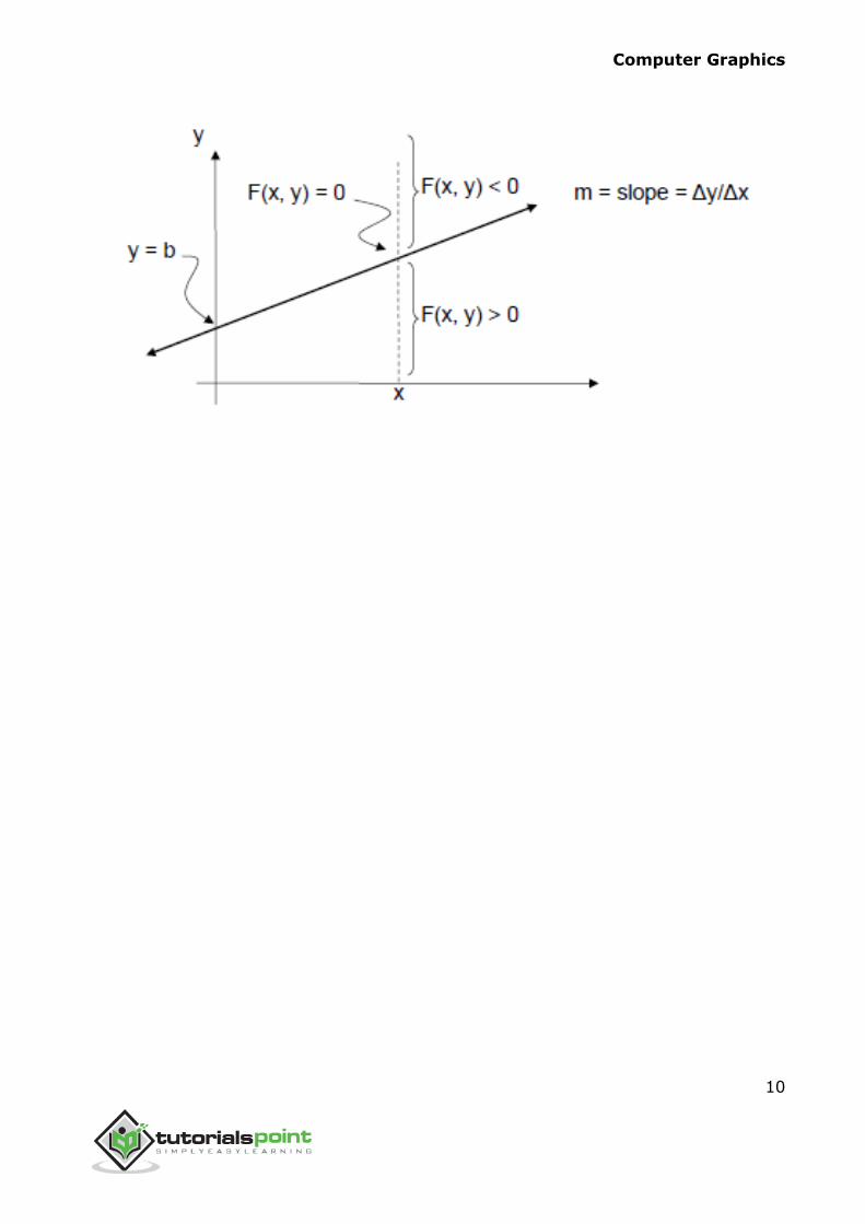
In order to check this, we need to consider the implicit equation:
F(x,y) = mx + b - y
For positive m at any given X,
If y is on the line, then F(x, y) = 0
If y is above the line, then F(x, y) < 0
If y is below the line, then F(x, y) > 0
Computer Graphics
10
Computer Graphics
11
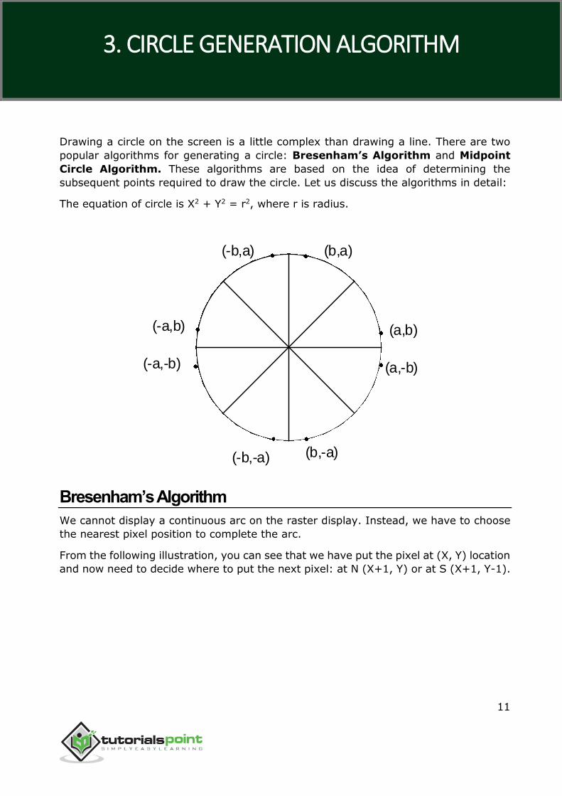
Drawing a circle on the screen is a little complex than drawing a line. There are two
popular algorithms for generating a circle: Bresenham’s Algorithm and Midpoint
Circle Algorithm. These algorithms are based on the idea of determining the
subsequent points required to draw the circle. Let us discuss the algorithms in detail:
The equation of circle is X2 + Y2 = r2, where r is radius.
Bresenham’s Algorithm
We cannot display a continuous arc on the raster display. Instead, we have to choose
the nearest pixel position to complete the arc.
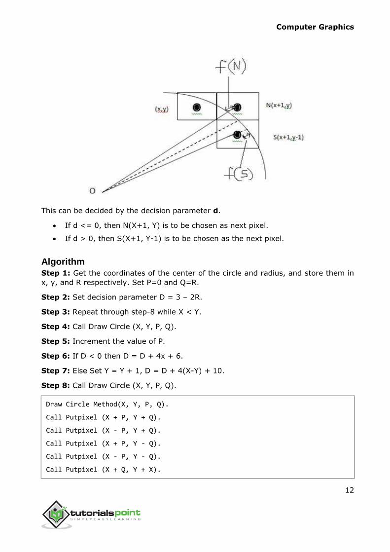
From the following illustration, you can see that we have put the pixel at (X, Y) location
and now need to decide where to put the next pixel: at N (X+1, Y) or at S (X+1, Y-1).
(a,b)
(b,a)
(a,-b)
(b,-a)
(-a,-b)
(-a,b)
(-b,-a)
(-b,a)
3. CIRCLE GENERATION ALGORITHM
Computer Graphics
12
This can be decided by the decision parameter d.
If d <= 0, then N(X+1, Y) is to be chosen as next pixel.
If d > 0, then S(X+1, Y-1) is to be chosen as the next pixel.
Algorithm
Step 1: Get the coordinates of the center of the circle and radius, and store them in
x, y, and R respectively. Set P=0 and Q=R.
Step 2: Set decision parameter D = 3 – 2R.
Step 3: Repeat through step-8 while X < Y.
Step 4: Call Draw Circle (X, Y, P, Q).
Step 5: Increment the value of P.
Step 6: If D < 0 then D = D + 4x + 6.
Step 7: Else Set Y = Y + 1, D = D + 4(X-Y) + 10.
Step 8: Call Draw Circle (X, Y, P, Q).
Draw Circle Method(X, Y, P, Q).
Call Putpixel (X + P, Y + Q).
Call Putpixel (X - P, Y + Q).
Call Putpixel (X + P, Y - Q).
Call Putpixel (X - P, Y - Q).
Call Putpixel (X + Q, Y + X).
Computer Graphics
13
Call Putpixel (X - Q, Y + X).
Call Putpixel (X + Q, Y - X).
Call Putpixel (X - Q, Y - X).
Mid Point Algorithm
Step 1: Input radius r and circle center (xc, yc) and obtain the first point on the
circumference of the circle centered on the origin as
(x0, y0) = (0, r)
Step 2: Calculate the initial value of decision parameter as
P0 = 5/4 – r (See the following description for simplification of this equation.)
f(x, y) = x2 + y2 - r2 = 0
f(xi - 1/2 + e, yi + 1)
= (xi - 1/2 + e)2 + (yi + 1)2 - r2
= (xi- 1/2)2 + (yi + 1)2 - r2 + 2(xi - 1/2)e + e2
= f(xi - 1/2, yi + 1) + 2(xi - 1/2)e + e2 = 0
Computer Graphics
14
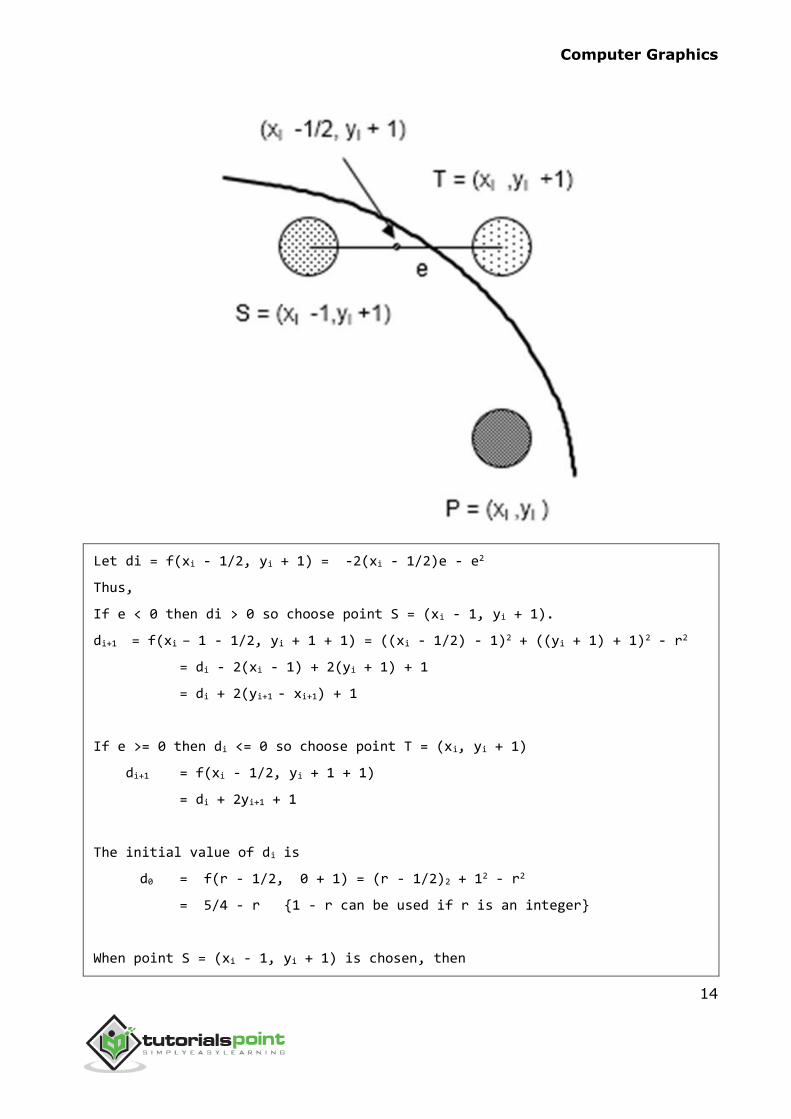
Let di = f(xi - 1/2, yi + 1) = -2(xi - 1/2)e - e2
Thus,
If e < 0 then di > 0 so choose point S = (xi - 1, yi + 1).
di+1 = f(xi – 1 - 1/2, yi + 1 + 1) = ((xi - 1/2) - 1)2 + ((yi + 1) + 1)2 - r2
= di - 2(xi - 1) + 2(yi + 1) + 1
= di + 2(yi+1 - xi+1) + 1
If e >= 0 then di <= 0 so choose point T = (xi, yi + 1)
di+1 = f(xi - 1/2, yi + 1 + 1)
= di + 2yi+1 + 1
The initial value of di is
d0 = f(r - 1/2, 0 + 1) = (r - 1/2)2 + 12 - r2
= 5/4 - r {1 - r can be used if r is an integer}
When point S = (xi - 1, yi + 1) is chosen, then
Computer Graphics
15
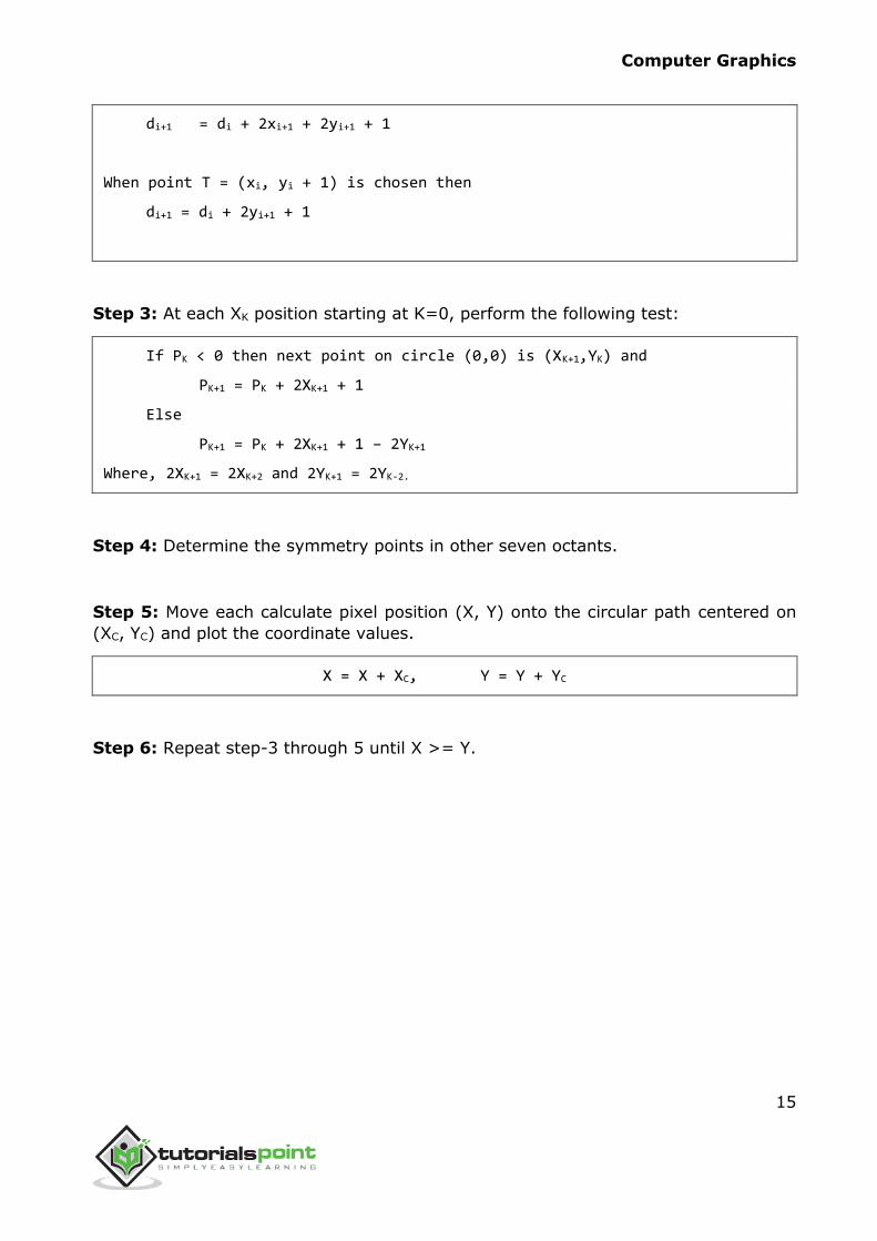
di+1 = di + 2xi+1 + 2yi+1 + 1
When point T = (xi, yi + 1) is chosen then
di+1 = di + 2yi+1 + 1
Step 3: At each XK position starting at K=0, perform the following test:
If PK < 0 then next point on circle (0,0) is (XK+1,YK) and
PK+1 = PK + 2XK+1 + 1
Else
PK+1 = PK + 2XK+1 + 1 – 2YK+1
Where, 2XK+1 = 2XK+2 and 2YK+1 = 2YK-2.
Step 4: Determine the symmetry points in other seven octants.
Step 5: Move each calculate pixel position (X, Y) onto the circular path centered on
(XC, YC) and plot the coordinate values.
X = X + XC, Y = Y + YC
Step 6: Repeat step-3 through 5 until X >= Y.
Computer Graphics
16
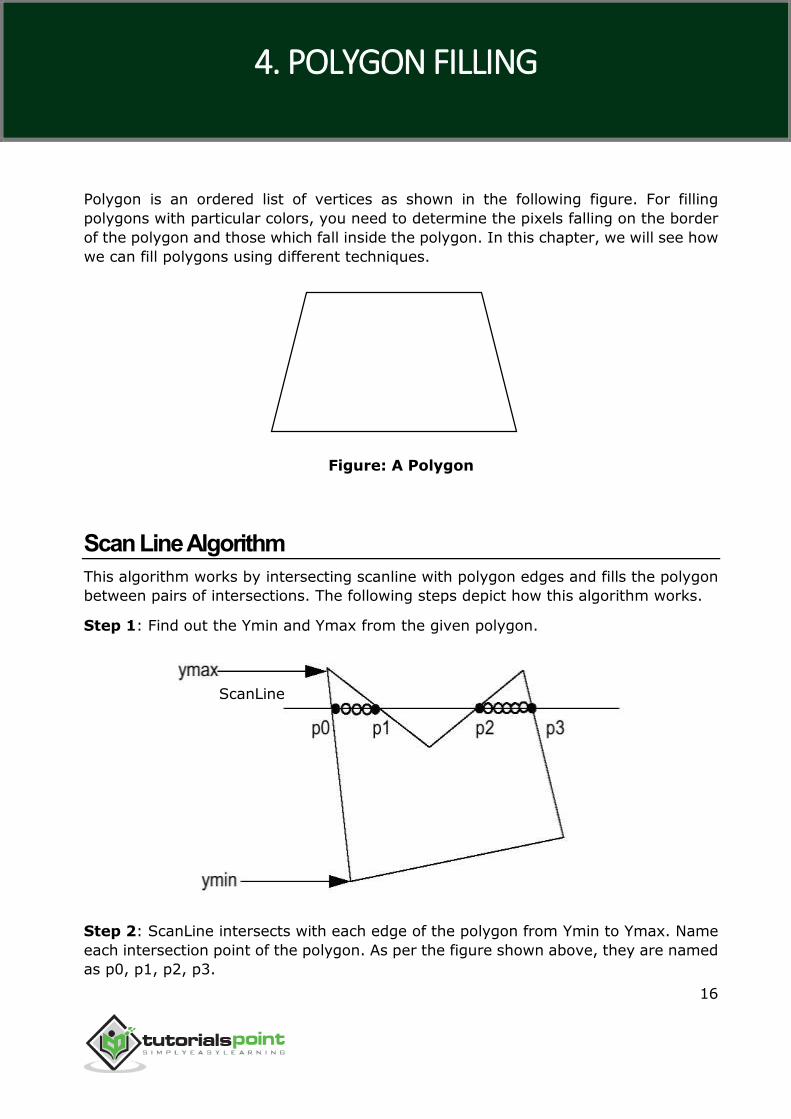
Polygon is an ordered list of vertices as shown in the following figure. For filling
polygons with particular colors, you need to determine the pixels falling on the border
of the polygon and those which fall inside the polygon. In this chapter, we will see how
we can fill polygons using different techniques.
Figure: A Polygon
Scan Line Algorithm
This algorithm works by intersecting scanline with polygon edges and fills the polygon
between pairs of intersections. The following steps depict how this algorithm works.
Step 1: Find out the Ymin and Ymax from the given polygon.
Step 2: ScanLine intersects with each edge of the polygon from Ymin to Ymax. Name
each intersection point of the polygon. As per the figure shown above, they are named
as p0, p1, p2, p3.
4. POLYGON FILLING
ScanLine
Computer Graphics
17
Step 3: Sort the intersection point in the increasing order of X coordinate i.e. (p0, p1),
(p1, p2), and (p2, p3).
Step 4: Fill all those pair of coordinates that are inside polygons and ignore the
alternate pairs.
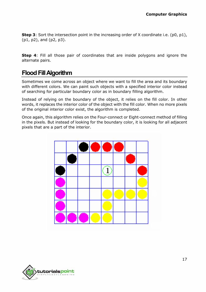
Flood Fill Algorithm
Sometimes we come across an object where we want to fill the area and its boundary
with different colors. We can paint such objects with a specified interior color instead
of searching for particular boundary color as in boundary filling algorithm.
Instead of relying on the boundary of the object, it relies on the fill color. In other
words, it replaces the interior color of the object with the fill color. When no more pixels
of the original interior color exist, the algorithm is completed.
Once again, this algorithm relies on the Four-connect or Eight-connect method of filling
in the pixels. But instead of looking for the boundary color, it is looking for all adjacent
pixels that are a part of the interior.
Computer Graphics
18
Boundary Fill Algorithm
The boundary fill algorithm works as its name. This algorithm picks a point inside an
object and starts to fill until it hits the boundary of the object. The color of the boundary
and the color that we fill should be different for this algorithm to work.
In this algorithm, we assume that color of the boundary is same for the entire object.
The boundary fill algorithm can be implemented by 4-connetected pixels or 8-
connected pixels.
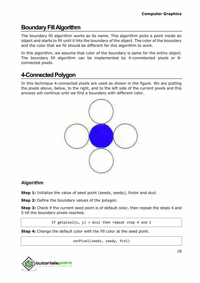
4-Connected Polygon
In this technique 4-connected pixels are used as shown in the figure. We are putting
the pixels above, below, to the right, and to the left side of the current pixels and this
process will continue until we find a boundary with different color.
Algorithm
Step 1: Initialize the value of seed point (seedx, seedy), fcolor and dcol.
Step 2: Define the boundary values of the polygon.
Step 3: Check if the current seed point is of default color, then repeat the steps 4 and
5 till the boundary pixels reached.
If getpixel(x, y) = dcol then repeat step 4 and 5
Step 4: Change the default color with the fill color at the seed point.
setPixel(seedx, seedy, fcol)
Computer Graphics
19
Step 5: Recursively follow the procedure with four neighborhood points.
FloodFill (seedx – 1, seedy, fcol, dcol)
FloodFill (seedx + 1, seedy, fcol, dcol)
FloodFill (seedx, seedy - 1, fcol, dcol)
FloodFill (seedx – 1, seedy + 1, fcol, dcol)
Step 6: Exit
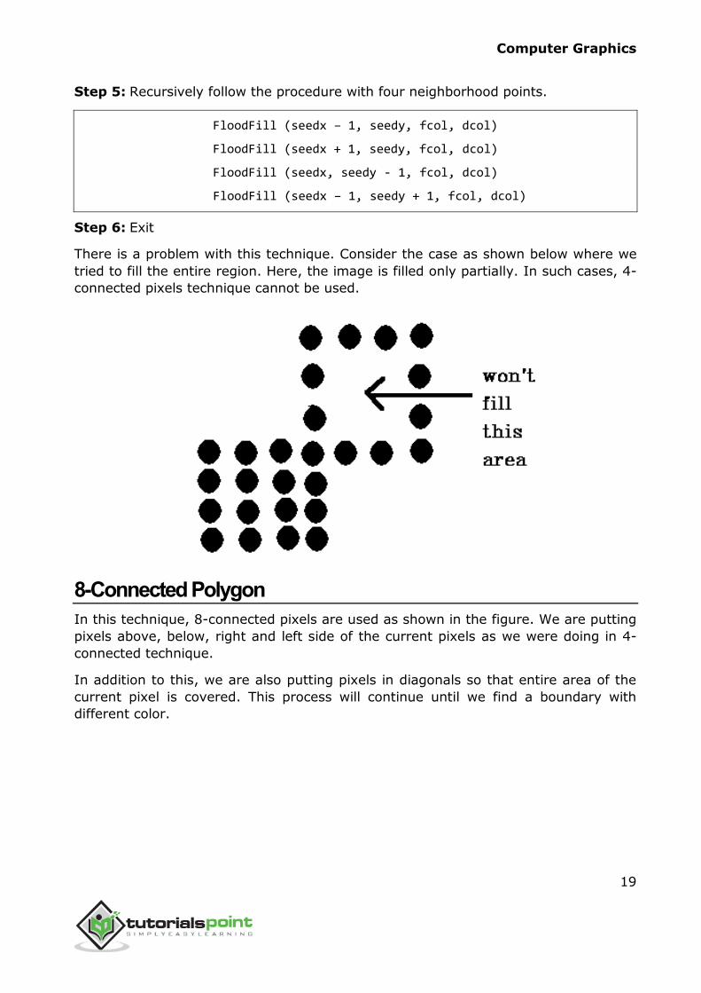
There is a problem with this technique. Consider the case as shown below where we
tried to fill the entire region. Here, the image is filled only partially. In such cases, 4-
connected pixels technique cannot be used.
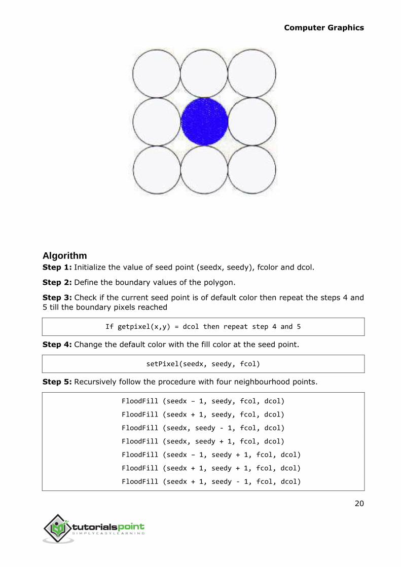
8-Connected Polygon
In this technique, 8-connected pixels are used as shown in the figure. We are putting
pixels above, below, right and left side of the current pixels as we were doing in 4-
connected technique.
In addition to this, we are also putting pixels in diagonals so that entire area of the
current pixel is covered. This process will continue until we find a boundary with
different color.
Computer Graphics
20
Algorithm Step 1: Initialize the value of seed point (seedx, seedy), fcolor and dcol.
Step 2: Define the boundary values of the polygon.
Step 3: Check if the current seed point is of default color then repeat the steps 4 and
5 till the boundary pixels reached
If getpixel(x,y) = dcol then repeat step 4 and 5
Step 4: Change the default color with the fill color at the seed point.
setPixel(seedx, seedy, fcol)
Step 5: Recursively follow the procedure with four neighbourhood points.
FloodFill (seedx – 1, seedy, fcol, dcol)
FloodFill (seedx + 1, seedy, fcol, dcol)
FloodFill (seedx, seedy - 1, fcol, dcol)
FloodFill (seedx, seedy + 1, fcol, dcol)
FloodFill (seedx – 1, seedy + 1, fcol, dcol)
FloodFill (seedx + 1, seedy + 1, fcol, dcol)
FloodFill (seedx + 1, seedy - 1, fcol, dcol)
Computer Graphics
21
FloodFill (seedx – 1, seedy - 1, fcol, dcol)
Step 6: Exit
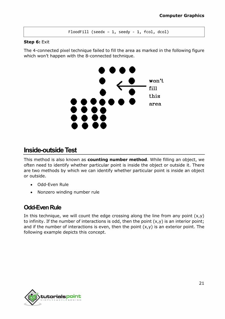
The 4-connected pixel technique failed to fill the area as marked in the following figure
which won’t happen with the 8-connected technique.
Inside-outside Test
This method is also known as counting number method. While filling an object, we
often need to identify whether particular point is inside the object or outside it. There
are two methods by which we can identify whether particular point is inside an object
or outside.
Odd-Even Rule
Nonzero winding number rule
Odd-Even Rule
In this technique, we will count the edge crossing along the line from any point (x,y)
to infinity. If the number of interactions is odd, then the point (x,y) is an interior point;
and if the number of interactions is even, then the point (x,y) is an exterior point. The
following example depicts this concept.
Computer Graphics
22
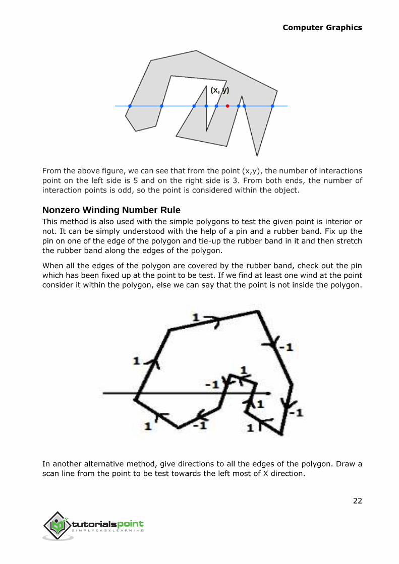
From the above figure, we can see that from the point (x,y), the number of interactions
point on the left side is 5 and on the right side is 3. From both ends, the number of
interaction points is odd, so the point is considered within the object.
Nonzero Winding Number Rule This method is also used with the simple polygons to test the given point is interior or
not. It can be simply understood with the help of a pin and a rubber band. Fix up the
pin on one of the edge of the polygon and tie-up the rubber band in it and then stretch
the rubber band along the edges of the polygon.
When all the edges of the polygon are covered by the rubber band, check out the pin
which has been fixed up at the point to be test. If we find at least one wind at the point
consider it within the polygon, else we can say that the point is not inside the polygon.
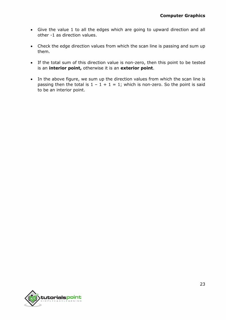
In another alternative method, give directions to all the edges of the polygon. Draw a
scan line from the point to be test towards the left most of X direction.
(x, y)
Computer Graphics
23
Give the value 1 to all the edges which are going to upward direction and all
other -1 as direction values.
Check the edge direction values from which the scan line is passing and sum up
them.
If the total sum of this direction value is non-zero, then this point to be tested
is an interior point, otherwise it is an exterior point.
In the above figure, we sum up the direction values from which the scan line is
passing then the total is 1 – 1 + 1 = 1; which is non-zero. So the point is said
to be an interior point.
Computer Graphics
24
The primary use of clipping in computer graphics is to remove objects, lines, or line
segments that are outside the viewing pane. The viewing transformation is insensitive
to the position of points relative to the viewing volume – especially those points behind
the viewer – and it is necessary to remove these points before generating the view.
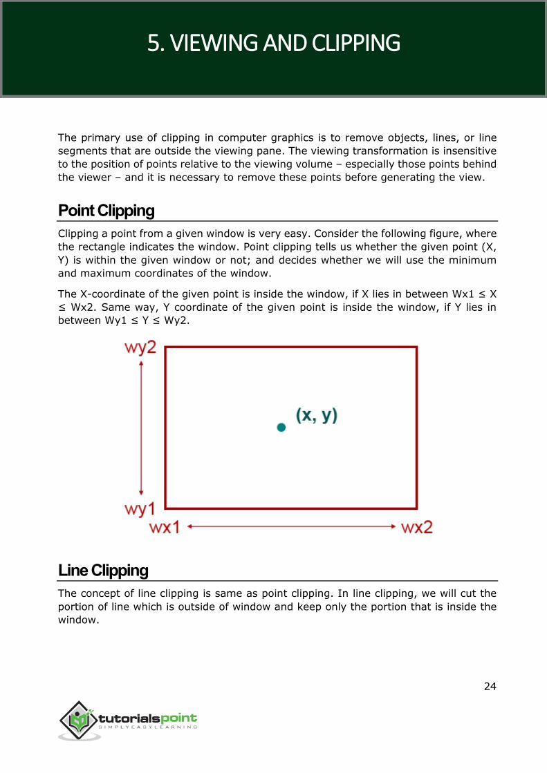
Point Clipping
Clipping a point from a given window is very easy. Consider the following figure, where
the rectangle indicates the window. Point clipping tells us whether the given point (X,
Y) is within the given window or not; and decides whether we will use the minimum
and maximum coordinates of the window.
The X-coordinate of the given point is inside the window, if X lies in between Wx1 ≤ X
≤ Wx2. Same way, Y coordinate of the given point is inside the window, if Y lies in
between Wy1 ≤ Y ≤ Wy2.
Line Clipping
The concept of line clipping is same as point clipping. In line clipping, we will cut the
portion of line which is outside of window and keep only the portion that is inside the
window.
5. VIEWING AND CLIPPING
Computer Graphics
25
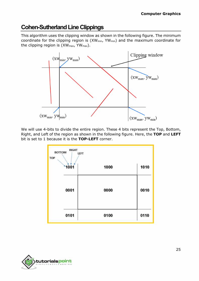
Cohen-Sutherland Line Clippings
This algorithm uses the clipping window as shown in the following figure. The minimum
coordinate for the clipping region is (XWmin, YWmin) and the maximum coordinate for
the clipping region is (XWmax, YWmax).
We will use 4-bits to divide the entire region. These 4 bits represent the Top, Bottom,
Right, and Left of the region as shown in the following figure. Here, the TOP and LEFT
bit is set to 1 because it is the TOP-LEFT corner.
Computer Graphics
26
There are 3 possibilities for the line:
1. Line can be completely inside the window (This line should be accepted).
2. Line can be completely outside of the window (This line will be completely
removed from the region).
3. Line can be partially inside the window (We will find intersection point and draw
only that portion of line that is inside region).
Algorithm Step 1: Assign a region code for each endpoints.
Step 2: If both endpoints have a region code 0000 then accept this line.
Step 3: Else, perform the logical AND operation for both region codes.
Step 3.1: If the result is not 0000, then reject the line.
Step 3.2: Else you need clipping.
Step 3.2.1: Choose an endpoint of the line that is outside the window.
Step 3.2.2: Find the intersection point at the window boundary (base on region
code).
Step 3.2.3: Replace endpoint with the intersection point and update the region
code.
Step 3.2.4: Repeat step 2 until we find a clipped line either trivially accepted or
trivially rejected.
Step-4: Repeat step 1 for other lines.
Computer Graphics
27
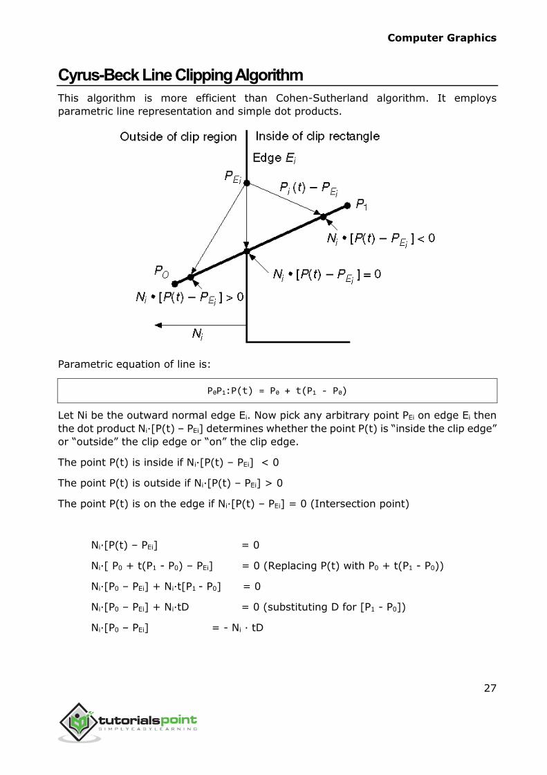
Cyrus-Beck Line Clipping Algorithm
This algorithm is more efficient than Cohen-Sutherland algorithm. It employs
parametric line representation and simple dot products.
Parametric equation of line is:
P0P1:P(t) = P0 + t(P1 - P0)
Let Ni be the outward normal edge Ei. Now pick any arbitrary point PEi on edge Ei then
the dot product Ni∙[P(t) – PEi] determines whether the point P(t) is “inside the clip edge”
or “outside” the clip edge or “on” the clip edge.
The point P(t) is inside if Ni∙[P(t) – PEi] < 0
The point P(t) is outside if Ni∙[P(t) – PEi] > 0
The point P(t) is on the edge if Ni∙[P(t) – PEi] = 0 (Intersection point)
Ni∙[P(t) – PEi] = 0
Ni∙[ P0 + t(P1 - P0) – PEi] = 0 (Replacing P(t) with P0 + t(P1 - P0))
Ni∙[P0 – PEi] + Ni∙t[P1 - P0] = 0
Ni∙[P0 – PEi] + Ni∙tD = 0 (substituting D for [P1 - P0])
Ni∙[P0 – PEi] = - Ni ∙ tD
Computer Graphics
28
The equation for t becomes,
t = N𝑖 ∙ [P0 – PEi]
−N𝑖 ∙ D
It is valid for the following conditions:
1. Ni ≠ 0 (error cannot happen)
2. D ≠ 0 (P1 ≠ P0)
3. Ni∙D ≠ 0 (P0P1 not parallel to Ei)
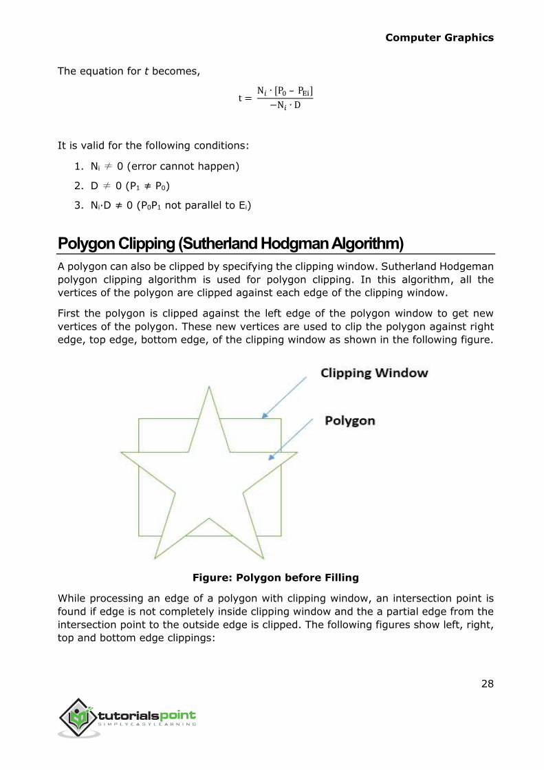
Polygon Clipping (Sutherland Hodgman Algorithm)
A polygon can also be clipped by specifying the clipping window. Sutherland Hodgeman
polygon clipping algorithm is used for polygon clipping. In this algorithm, all the
vertices of the polygon are clipped against each edge of the clipping window.
First the polygon is clipped against the left edge of the polygon window to get new
vertices of the polygon. These new vertices are used to clip the polygon against right
edge, top edge, bottom edge, of the clipping window as shown in the following figure.
Figure: Polygon before Filling
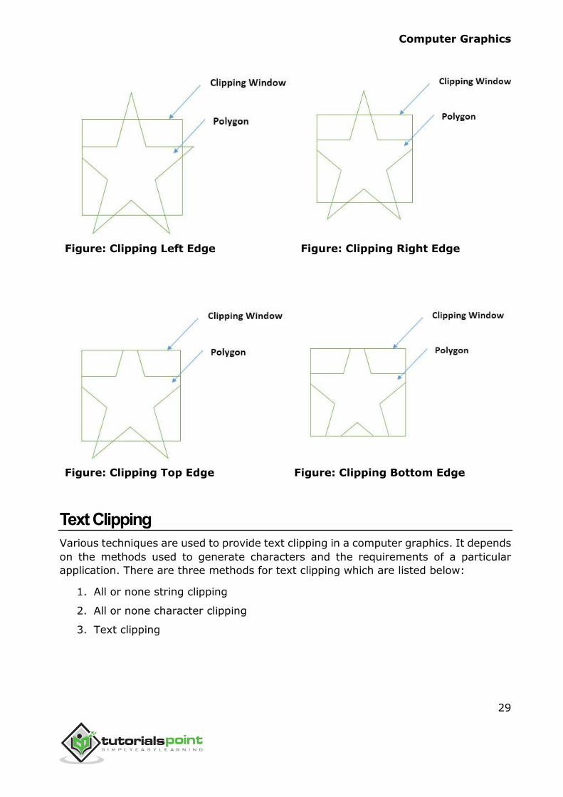
While processing an edge of a polygon with clipping window, an intersection point is
found if edge is not completely inside clipping window and the a partial edge from the
intersection point to the outside edge is clipped. The following figures show left, right,
top and bottom edge clippings:
Computer Graphics
29
Figure: Clipping Left Edge Figure: Clipping Right Edge
Figure: Clipping Top Edge Figure: Clipping Bottom Edge
Text Clipping
Various techniques are used to provide text clipping in a computer graphics. It depends
on the methods used to generate characters and the requirements of a particular
application. There are three methods for text clipping which are listed below:
1. All or none string clipping
2. All or none character clipping
3. Text clipping
Computer Graphics
30
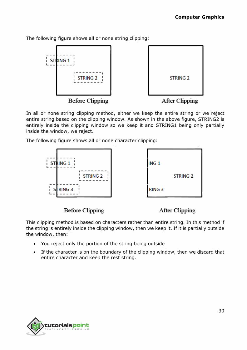
The following figure shows all or none string clipping:
In all or none string clipping method, either we keep the entire string or we reject
entire string based on the clipping window. As shown in the above figure, STRING2 is
entirely inside the clipping window so we keep it and STRING1 being only partially
inside the window, we reject.
The following figure shows all or none character clipping:
This clipping method is based on characters rather than entire string. In this method if
the string is entirely inside the clipping window, then we keep it. If it is partially outside
the window, then:
You reject only the portion of the string being outside
If the character is on the boundary of the clipping window, then we discard that
entire character and keep the rest string.
Computer Graphics
31
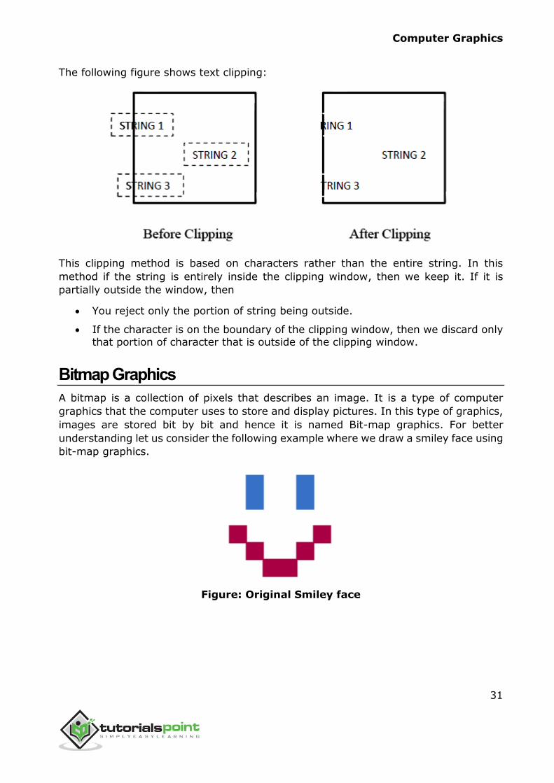
The following figure shows text clipping:
This clipping method is based on characters rather than the entire string. In this
method if the string is entirely inside the clipping window, then we keep it. If it is
partially outside the window, then
You reject only the portion of string being outside.
If the character is on the boundary of the clipping window, then we discard only
that portion of character that is outside of the clipping window.
Bitmap Graphics
A bitmap is a collection of pixels that describes an image. It is a type of computer
graphics that the computer uses to store and display pictures. In this type of graphics,
images are stored bit by bit and hence it is named Bit-map graphics. For better
understanding let us consider the following example where we draw a smiley face using
bit-map graphics.
Figure: Original Smiley face
Computer Graphics
32
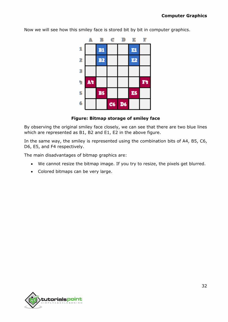
Now we will see how this smiley face is stored bit by bit in computer graphics.
Figure: Bitmap storage of smiley face
By observing the original smiley face closely, we can see that there are two blue lines
which are represented as B1, B2 and E1, E2 in the above figure.
In the same way, the smiley is represented using the combination bits of A4, B5, C6,
D6, E5, and F4 respectively.
The main disadvantages of bitmap graphics are:
We cannot resize the bitmap image. If you try to resize, the pixels get blurred.
Colored bitmaps can be very large.
Computer Graphics
33
Transformation means changing some graphics into something else by applying rules.
We can have various types of transformations such as translation, scaling up or down,
rotation, shearing, etc. When a transformation takes place on a 2D plane, it is called
2D transformation.
Transformations play an important role in computer graphics to reposition the graphics
on the screen and change their size or orientation.
Homogenous Coordinates
To perform a sequence of transformation such as translation followed by rotation and
scaling, we need to follow a sequential process:
1. Translate the coordinates,
2. Rotate the translated coordinates, and then
3. Scale the rotated coordinates to complete the composite transformation.
To shorten this process, we have to use 3×3 transformation matrix instead of 2×2
transformation matrix. To convert a 2×2 matrix to 3×3 matrix, we have to add an
extra dummy coordinate W.
In this way, we can represent the point by 3 numbers instead of 2 numbers, which is
called Homogenous Coordinate system. In this system, we can represent all the
transformation equations in matrix multiplication. Any Cartesian point P(X, Y) can be
converted to homogenous coordinates by P’ (Xh, Yh, h).
Translation
A translation moves an object to a different position on the screen. You can translate
a point in 2D by adding translation coordinate (tx, ty) to the original coordinate (X, Y)
to get the new coordinate (X’, Y’).
6. 2D TRANSFORMATION
Computer Graphics
34
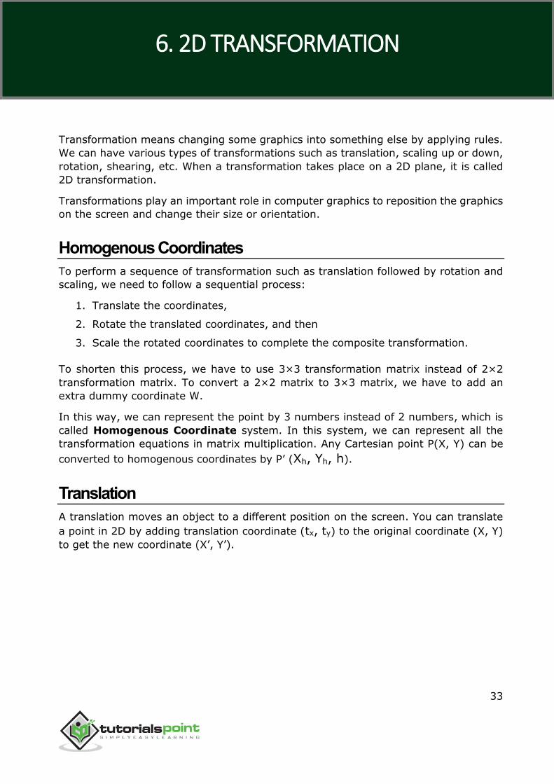
From the above figure, you can write that:
X’ = X + tx
Y’ = Y + ty
The pair (tx, ty) is called the translation vector or shift vector. The above equations
can also be represented using the column vectors.
𝑃 = [𝑋𝑌] 𝑃′ = [
𝑋′
𝑌′] 𝑇 = [
𝑡𝑥
𝑡𝑦]
We can write it as:
P’ = P + T
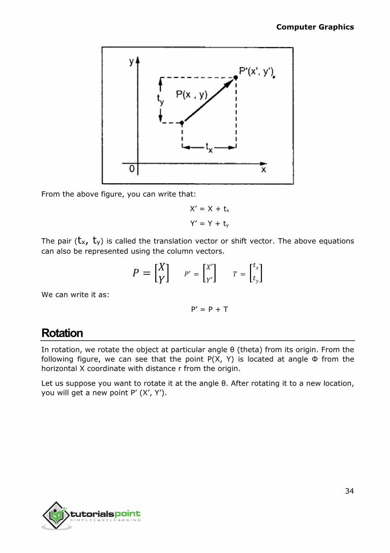
Rotation
In rotation, we rotate the object at particular angle θ (theta) from its origin. From the
following figure, we can see that the point P(X, Y) is located at angle Φ from the
horizontal X coordinate with distance r from the origin.
Let us suppose you want to rotate it at the angle θ. After rotating it to a new location,
you will get a new point P’ (X’, Y’).
Computer Graphics
35
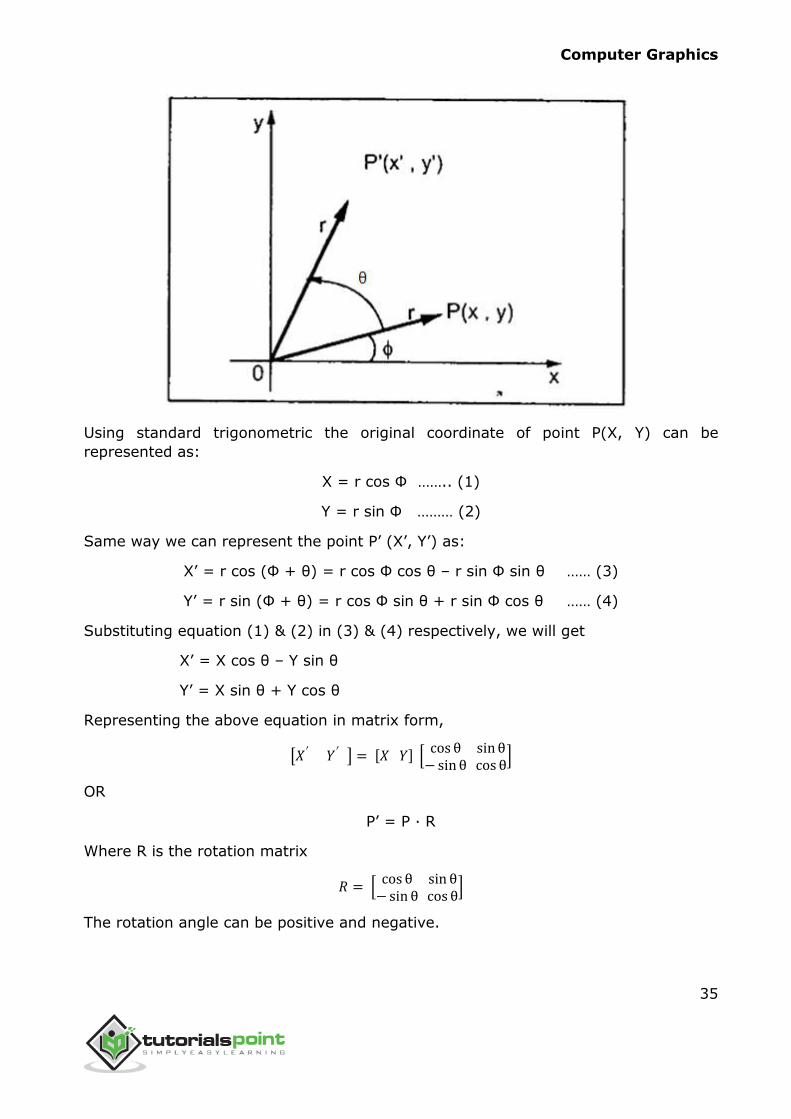
Using standard trigonometric the original coordinate of point P(X, Y) can be
represented as:
X = r cos Φ …….. (1)
Y = r sin Φ ……… (2)
Same way we can represent the point P’ (X’, Y’) as:
X’ = r cos (Φ + θ) = r cos Φ cos θ – r sin Φ sin θ …… (3)
Y’ = r sin (Φ + θ) = r cos Φ sin θ + r sin Φ cos θ …… (4)
Substituting equation (1) & (2) in (3) & (4) respectively, we will get
X’ = X cos θ – Y sin θ
Y’ = X sin θ + Y cos θ
Representing the above equation in matrix form,
[𝑋′ 𝑌′] = [𝑋 𝑌] [cos θ
− sinθ sin θ cos θ
]
OR
P’ = P ∙ R
Where R is the rotation matrix
𝑅 = [cos θ
− sin θ sin θ cos θ
]
The rotation angle can be positive and negative.
Computer Graphics
36
For positive rotation angle, we can use the above rotation matrix. However, for
negative angle rotation, the matrix will change as shown below:
𝑅 = [cos (−θ)−sin(−θ)
sin(−θ) cos(−θ)
]
= [cos θsin θ
− sin θ cos θ
] (∵ cos(−θ) = cos θ and sin(−θ) = −sin θ)
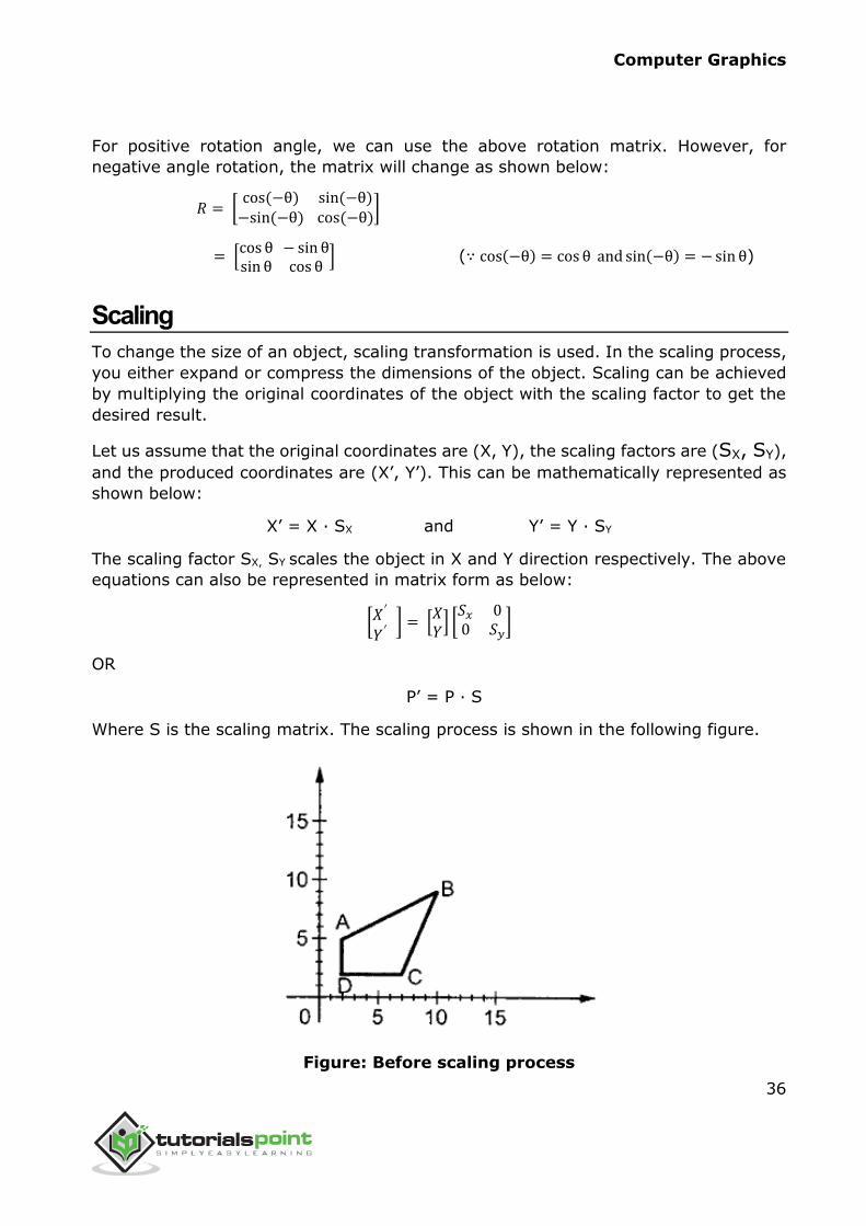
Scaling
To change the size of an object, scaling transformation is used. In the scaling process,
you either expand or compress the dimensions of the object. Scaling can be achieved
by multiplying the original coordinates of the object with the scaling factor to get the
desired result.
Let us assume that the original coordinates are (X, Y), the scaling factors are (SX, SY),
and the produced coordinates are (X’, Y’). This can be mathematically represented as
shown below:
X’ = X ∙ SX and Y’ = Y ∙ SY
The scaling factor SX, SY scales the object in X and Y direction respectively. The above
equations can also be represented in matrix form as below:
[𝑋′
𝑌′] = [
𝑋𝑌] [
𝑆𝑥 00 𝑆𝑦
]
OR
P’ = P ∙ S
Where S is the scaling matrix. The scaling process is shown in the following figure.
Figure: Before scaling process
Computer Graphics
37
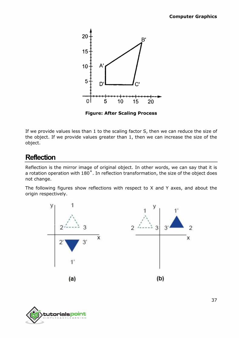
Figure: After Scaling Process
If we provide values less than 1 to the scaling factor S, then we can reduce the size of
the object. If we provide values greater than 1, then we can increase the size of the
object.
Reflection
Reflection is the mirror image of original object. In other words, we can say that it is
a rotation operation with 180˚. In reflection transformation, the size of the object does
not change.
The following figures show reflections with respect to X and Y axes, and about the
origin respectively.
Computer Graphics
38
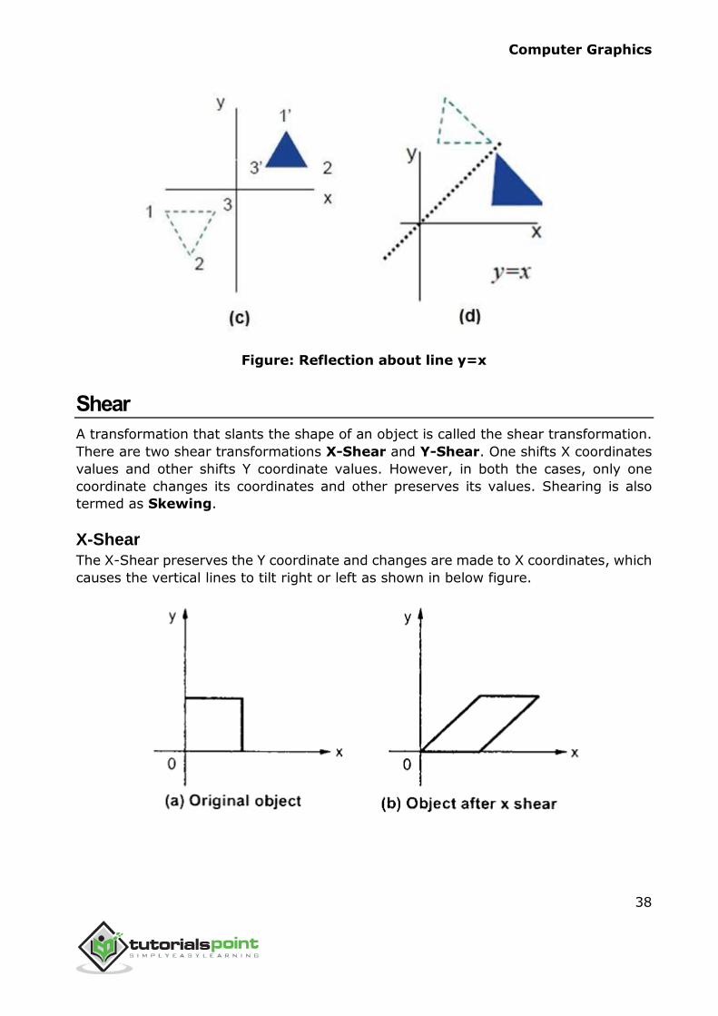
Figure: Reflection about line y=x
Shear
A transformation that slants the shape of an object is called the shear transformation.
There are two shear transformations X-Shear and Y-Shear. One shifts X coordinates
values and other shifts Y coordinate values. However, in both the cases, only one
coordinate changes its coordinates and other preserves its values. Shearing is also
termed as Skewing.
X-Shear The X-Shear preserves the Y coordinate and changes are made to X coordinates, which
causes the vertical lines to tilt right or left as shown in below figure.
Computer Graphics
39
The transformation matrix for X-Shear can be represented as:
𝑋𝑆ℎ = [1 0 0
Sh𝑥 1 00 0 1
]
X’ = X + Shx ∙ Y
Y’ = Y
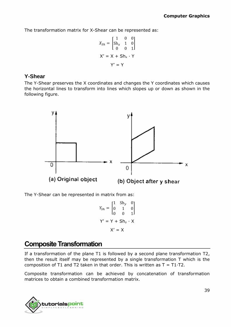
Y-Shear The Y-Shear preserves the X coordinates and changes the Y coordinates which causes
the horizontal lines to transform into lines which slopes up or down as shown in the
following figure.
The Y-Shear can be represented in matrix from as:
𝑌𝑆ℎ = [1 Sh𝑦 0
0 1 00 0 1
]
Y’ = Y + Shy ∙ X
X’ = X
Composite Transformation
If a transformation of the plane T1 is followed by a second plane transformation T2,
then the result itself may be represented by a single transformation T which is the
composition of T1 and T2 taken in that order. This is written as T = T1∙T2.
Composite transformation can be achieved by concatenation of transformation
matrices to obtain a combined transformation matrix.
Computer Graphics
40
A combined matrix:
[T][X] = [X] [T1] [T2] [T3] [T4] …. [Tn]
Where [Ti] is any combination of
Translation
Scaling
Shearing
Rotation
Reflection
The change in the order of transformation would lead to different results, as in general
matrix multiplication is not cumulative, that is [A] ∙ [B] ≠ [B] ∙ [A] and the order of
multiplication. The basic purpose of composing transformations is to gain efficiency by
applying a single composed transformation to a point, rather than applying a series of
transformation, one after another.
For example, to rotate an object about an arbitrary point (Xp, Yp), we have to carry
out three steps:
1. Translate point (Xp, Yp) to the origin.
2. Rotate it about the origin.
3. Finally, translate the center of rotation back where it belonged.
Computer Graphics
41
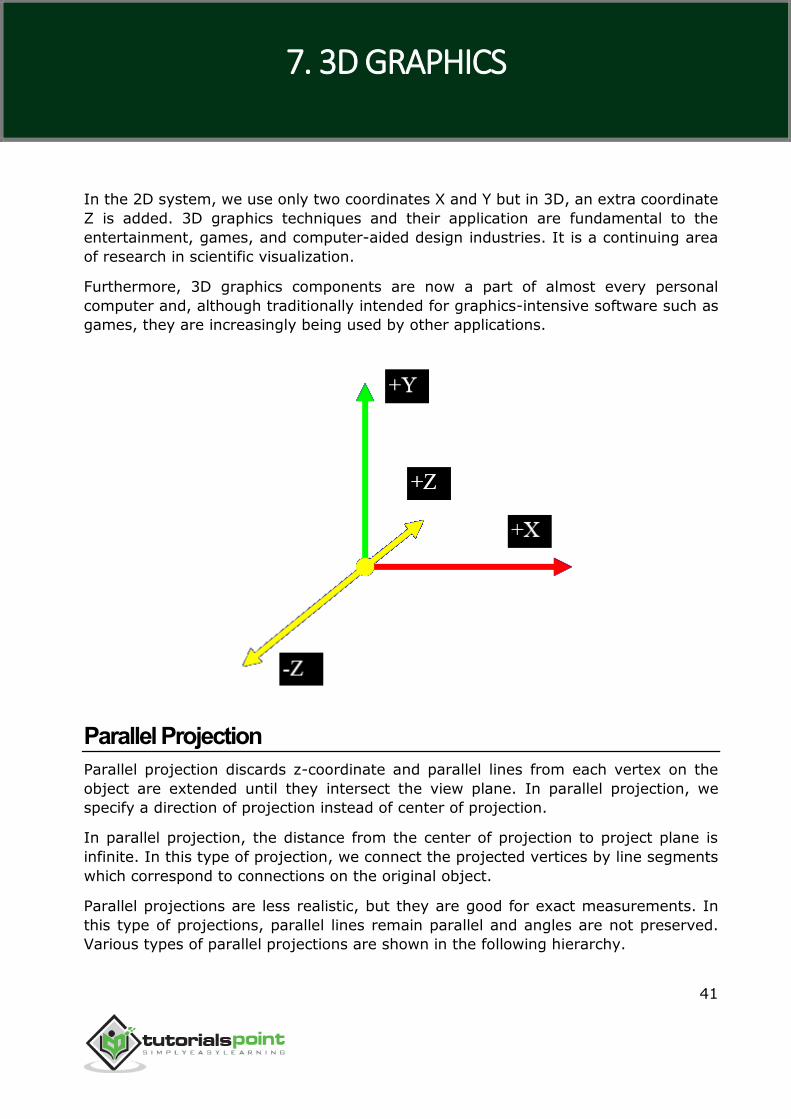
In the 2D system, we use only two coordinates X and Y but in 3D, an extra coordinate
Z is added. 3D graphics techniques and their application are fundamental to the
entertainment, games, and computer-aided design industries. It is a continuing area
of research in scientific visualization.
Furthermore, 3D graphics components are now a part of almost every personal
computer and, although traditionally intended for graphics-intensive software such as
games, they are increasingly being used by other applications.
Parallel Projection
Parallel projection discards z-coordinate and parallel lines from each vertex on the
object are extended until they intersect the view plane. In parallel projection, we
specify a direction of projection instead of center of projection.
In parallel projection, the distance from the center of projection to project plane is
infinite. In this type of projection, we connect the projected vertices by line segments
which correspond to connections on the original object.
Parallel projections are less realistic, but they are good for exact measurements. In
this type of projections, parallel lines remain parallel and angles are not preserved.
Various types of parallel projections are shown in the following hierarchy.
7. 3D GRAPHICS
Computer Graphics
42
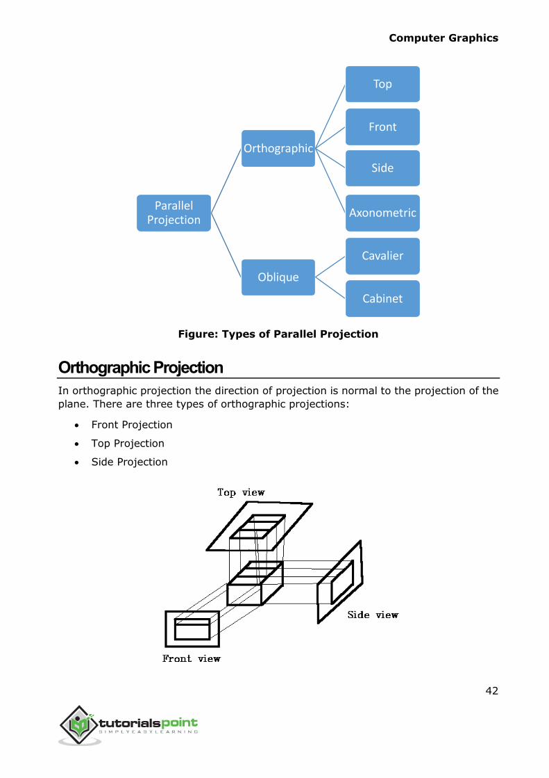
Figure: Types of Parallel Projection
Orthographic Projection
In orthographic projection the direction of projection is normal to the projection of the
plane. There are three types of orthographic projections:
Front Projection
Top Projection
Side Projection
Parallel Projection
Orthographic
Top
Front
Side
Axonometric
Oblique
Cavalier
Cabinet
Computer Graphics
43
Oblique Projection
In orthographic projection, the direction of projection is not normal to the projection
of plane. In oblique projection, we can view the object better than orthographic
projection.
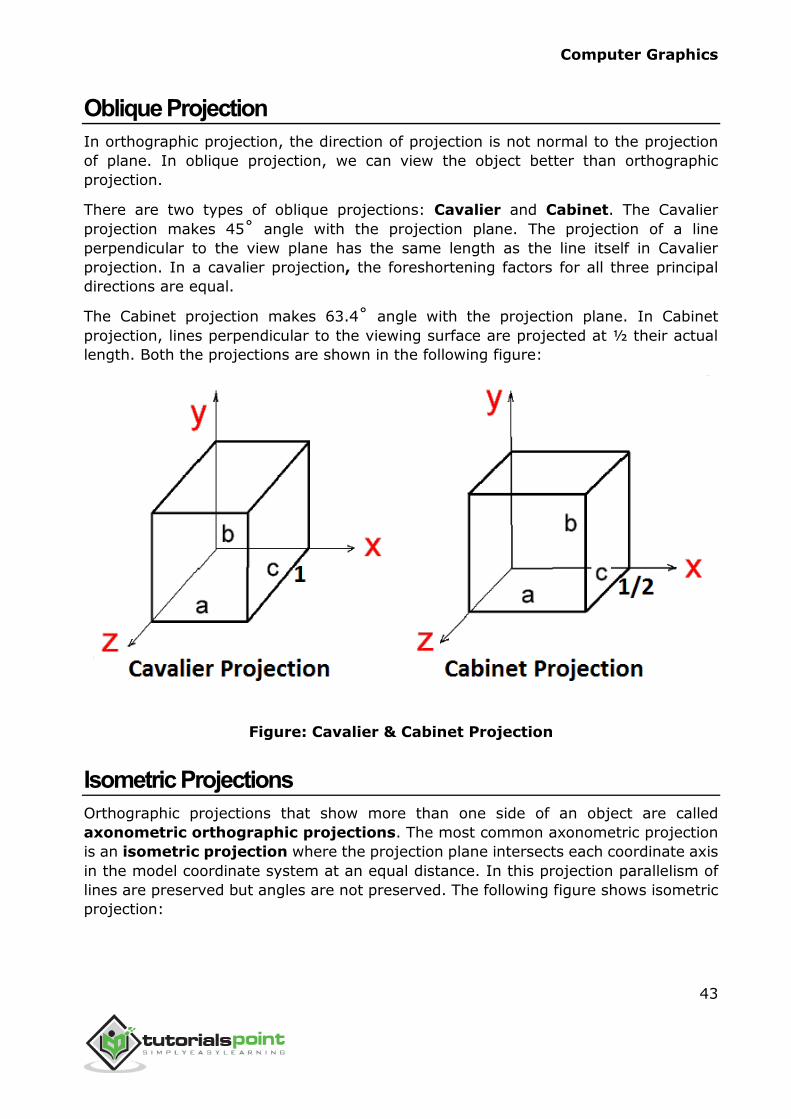
There are two types of oblique projections: Cavalier and Cabinet. The Cavalier
projection makes 45˚ angle with the projection plane. The projection of a line
perpendicular to the view plane has the same length as the line itself in Cavalier
projection. In a cavalier projection, the foreshortening factors for all three principal
directions are equal.
The Cabinet projection makes 63.4˚ angle with the projection plane. In Cabinet
projection, lines perpendicular to the viewing surface are projected at ½ their actual
length. Both the projections are shown in the following figure:
Figure: Cavalier & Cabinet Projection
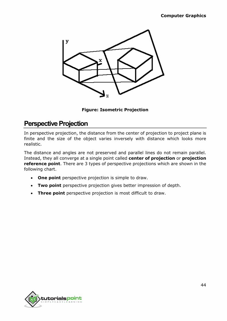
Isometric Projections
Orthographic projections that show more than one side of an object are called
axonometric orthographic projections. The most common axonometric projection
is an isometric projection where the projection plane intersects each coordinate axis
in the model coordinate system at an equal distance. In this projection parallelism of
lines are preserved but angles are not preserved. The following figure shows isometric
projection:
Computer Graphics
44
Figure: Isometric Projection
Perspective Projection
In perspective projection, the distance from the center of projection to project plane is
finite and the size of the object varies inversely with distance which looks more
realistic.
The distance and angles are not preserved and parallel lines do not remain parallel.
Instead, they all converge at a single point called center of projection or projection
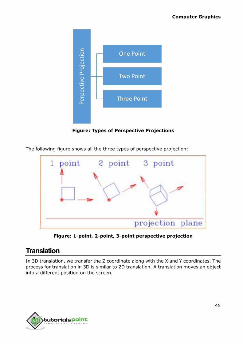
reference point. There are 3 types of perspective projections which are shown in the
following chart.
One point perspective projection is simple to draw.
Two point perspective projection gives better impression of depth.
Three point perspective projection is most difficult to draw.
Computer Graphics
45
Figure: Types of Perspective Projections
The following figure shows all the three types of perspective projection:
Figure: 1-point, 2-point, 3-point perspective projection
Translation
In 3D translation, we transfer the Z coordinate along with the X and Y coordinates. The
process for translation in 3D is similar to 2D translation. A translation moves an object
into a different position on the screen.
Perp
ecti
ve P
roje
ctio
n
One Point
Two Point
Three Point
Computer Graphics
46
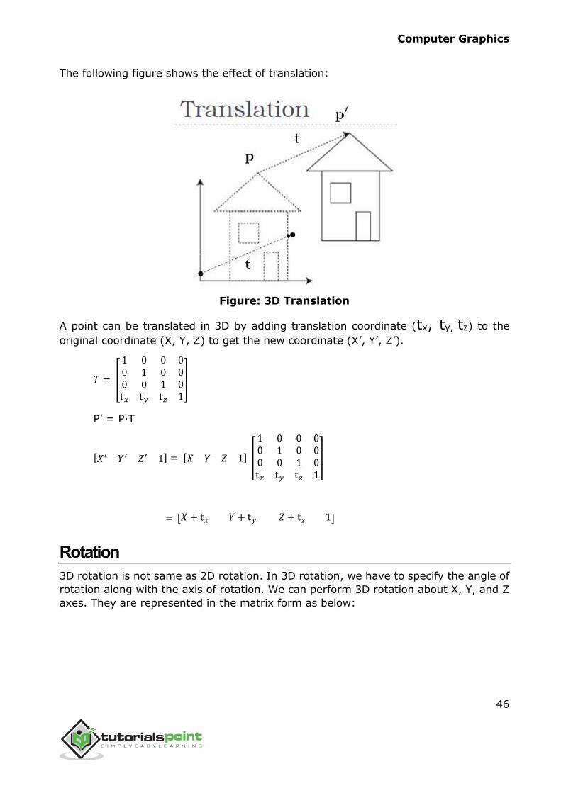
The following figure shows the effect of translation:
Figure: 3D Translation
A point can be translated in 3D by adding translation coordinate (tx, ty, tz) to the
original coordinate (X, Y, Z) to get the new coordinate (X’, Y’, Z’).
𝑇 = [
1 0 0 00 1 0 00 0 1 0t𝑥 t𝑦 t𝑧 1
]
P’ = P∙T
[𝑋′ 𝑌′ 𝑍′ 1] = [𝑋 𝑌 𝑍 1] [
1 0 0 00 1 0 00 0 1 0t𝑥 t𝑦 t𝑧 1
]
= [𝑋 + t𝑥 𝑌 + t𝑦 𝑍 + t𝑧 1]
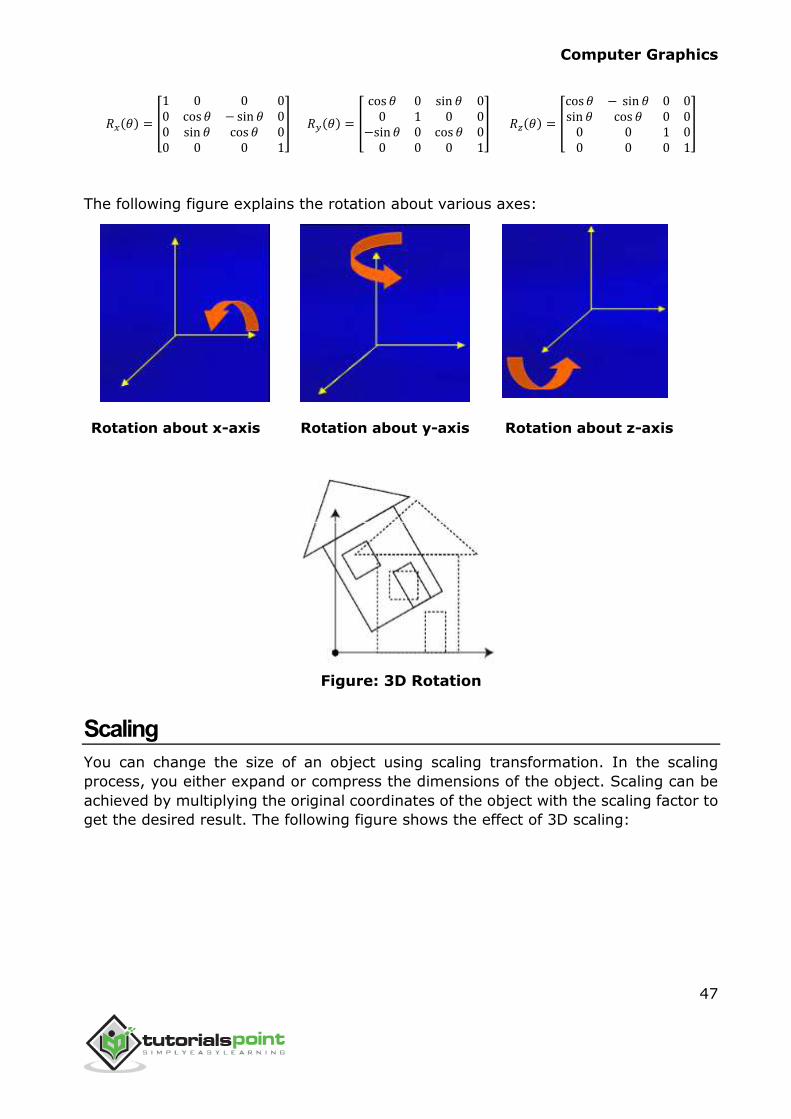
Rotation
3D rotation is not same as 2D rotation. In 3D rotation, we have to specify the angle of
rotation along with the axis of rotation. We can perform 3D rotation about X, Y, and Z
axes. They are represented in the matrix form as below:
Computer Graphics
47
𝑅𝑥(𝜃) = [
1 0 0 00 cos 𝜃 − sin 𝜃 00 sin 𝜃 cos 𝜃 00 0 0 1
] 𝑅𝑦(𝜃) = [
cos 𝜃 0 sin 𝜃 00 1 0 0
−sin 𝜃 0 cos 𝜃 00 0 0 1
] 𝑅𝑧(𝜃) = [
cos 𝜃 − sin 𝜃 0 0sin 𝜃 cos 𝜃 0 0
0 0 1 00 0 0 1
]
The following figure explains the rotation about various axes:
Rotation about x-axis
Rotation about y-axis
Rotation about z-axis
Figure: 3D Rotation
Scaling
You can change the size of an object using scaling transformation. In the scaling
process, you either expand or compress the dimensions of the object. Scaling can be
achieved by multiplying the original coordinates of the object with the scaling factor to
get the desired result. The following figure shows the effect of 3D scaling:
Computer Graphics
48
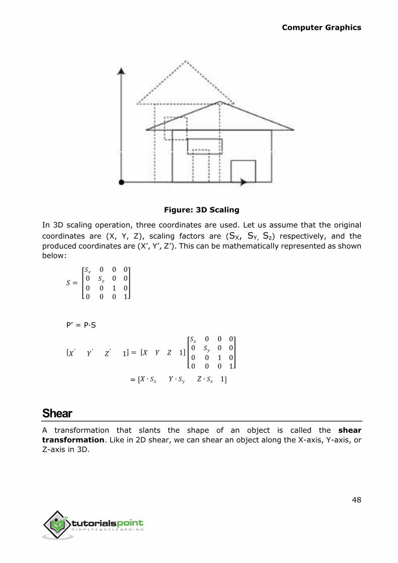
Figure: 3D Scaling
In 3D scaling operation, three coordinates are used. Let us assume that the original
coordinates are (X, Y, Z), scaling factors are (SX, SY, Sz) respectively, and the
produced coordinates are (X’, Y’, Z’). This can be mathematically represented as shown
below:
𝑆 = [
𝑆𝑥 0 0 00 𝑆𝑦 0 0
0 0 1 00 0 0 1
]
P’ = P∙S
[𝑋′ 𝑌′ 𝑍′ 1] = [𝑋 𝑌 𝑍 1] [
𝑆𝑥 0 0 00 𝑆𝑦 0 0
0 0 1 00 0 0 1
]
= [𝑋 ∙ 𝑆𝑥 𝑌 ∙ 𝑆𝑦 𝑍 ∙ 𝑆𝑧 1]
Shear
A transformation that slants the shape of an object is called the shear
transformation. Like in 2D shear, we can shear an object along the X-axis, Y-axis, or
Z-axis in 3D.
Computer Graphics
49
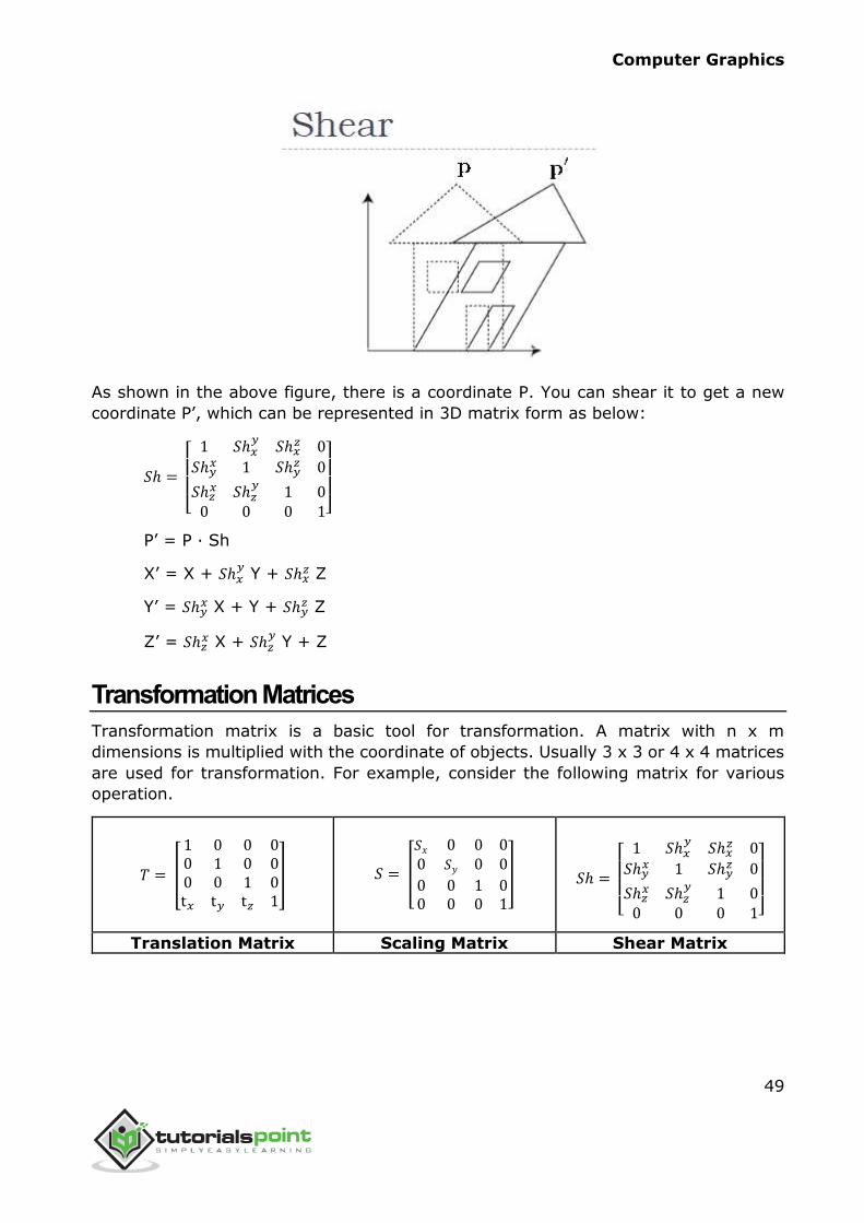
As shown in the above figure, there is a coordinate P. You can shear it to get a new
coordinate P’, which can be represented in 3D matrix form as below:
𝑆ℎ =
[
1 𝑆ℎ𝑥𝑦
𝑆ℎ𝑥𝑧 0
𝑆ℎ𝑦𝑥 1 𝑆ℎ𝑦
𝑧 0
𝑆ℎ𝑧𝑥 𝑆ℎ𝑧
𝑦1 0
0 0 0 1]
P’ = P ∙ Sh
X’ = X + 𝑆ℎ𝑥𝑦 Y + 𝑆ℎ𝑥
𝑧 Z
Y’ = 𝑆ℎ𝑦𝑥 X + Y + 𝑆ℎ𝑦
𝑧 Z
Z’ = 𝑆ℎ𝑧𝑥 X + 𝑆ℎ𝑧
𝑦 Y + Z
Transformation Matrices
Transformation matrix is a basic tool for transformation. A matrix with n x m
dimensions is multiplied with the coordinate of objects. Usually 3 x 3 or 4 x 4 matrices
are used for transformation. For example, consider the following matrix for various
operation.
𝑇 = [
1 0 0 00 1 0 00 0 1 0t𝑥 t𝑦 t𝑧 1
]
𝑆 = [
𝑆𝑥 0 0 00 𝑆𝑦 0 0
0 0 1 00 0 0 1
]
𝑆ℎ =
[
1 𝑆ℎ𝑥𝑦
𝑆ℎ𝑥𝑧 0
𝑆ℎ𝑦𝑥 1 𝑆ℎ𝑦
𝑧 0
𝑆ℎ𝑧𝑥 𝑆ℎ𝑧
𝑦1 0
0 0 0 1]
Translation Matrix Scaling Matrix Shear Matrix

Computer Graphics
50
𝑅𝑥(𝜃) = [
1 0 0 00 cos 𝜃 − sin 𝜃 00 sin 𝜃 cos 𝜃 00 0 0 1
]
𝑅𝑦(𝜃) = [
cos 𝜃 0 sin 𝜃 00 1 0 0
−sin 𝜃 0 cos 𝜃 00 0 0 1
]
𝑅𝑧(𝜃) = [
cos 𝜃 − sin 𝜃 0 0sin 𝜃 cos 𝜃 0 0
0 0 1 00 0 0 1
]
Rotation Matrix
Computer Graphics
51
In computer graphics, we often need to draw different types of objects onto the screen.
Objects are not flat all the time and we need to draw curves many times to draw an
object.
Types of Curves
A curve is an infinitely large set of points. Each point has two neighbors except
endpoints. Curves can be broadly classified into three categories: explicit, implicit,
and parametric curves.
Implicit Curves
Implicit curve representations define the set of points on a curve by employing a
procedure that can test to see if a point in on the curve. Usually, an implicit curve is
defined by an implicit function of the form:
f(x, y) = 0
It can represent multivalued curves (multiple y values for an x value). A common
example is the circle, whose implicit representation is
x2 + y2 − R2 = 0
Explicit Curves
A mathematical function y = f(x) can be plotted as a curve. Such a function is the
explicit representation of the curve. The explicit representation is not general, since it
cannot represent vertical lines and is also single-valued. For each value of x, only a
single value of y is normally computed by the function.
Parametric Curves
Curves having parametric form are called parametric curves. The explicit and implicit
curve representations can be used only when the function is known. In practice the
parametric curves are used. A two-dimensional parametric curve has the following
form:
P(t) = f(t), g(t) or P(t) = x(t), y(t)
The functions f and g become the (x, y) coordinates of any point on the curve, and the
points are obtained when the parameter t is varied over a certain interval [a, b],
normally [0, 1].
8. CURVES
Computer Graphics
52
Bezier Curves
Bezier curve is discovered by the French engineer Pierre Bézier. These curves can be
generated under the control of other points. Approximate tangents by using control
points are used to generate curve. The Bezier curve can be represented mathematically
as:
∑ 𝑃𝑖
𝑛
𝑘=0
𝐵𝑖𝑛(𝑡)
Where 𝑃𝑖 is the set of points and 𝐵𝑖𝑛(𝑡) represents the Bernstein polynomials which
are given by:
𝐵𝑖𝑛(𝑡) = (
𝑛
𝑖) (1 − 𝑡)𝑛−𝑖𝑡𝑖
Where n is the polynomial degree, i is the index, and t is the variable.
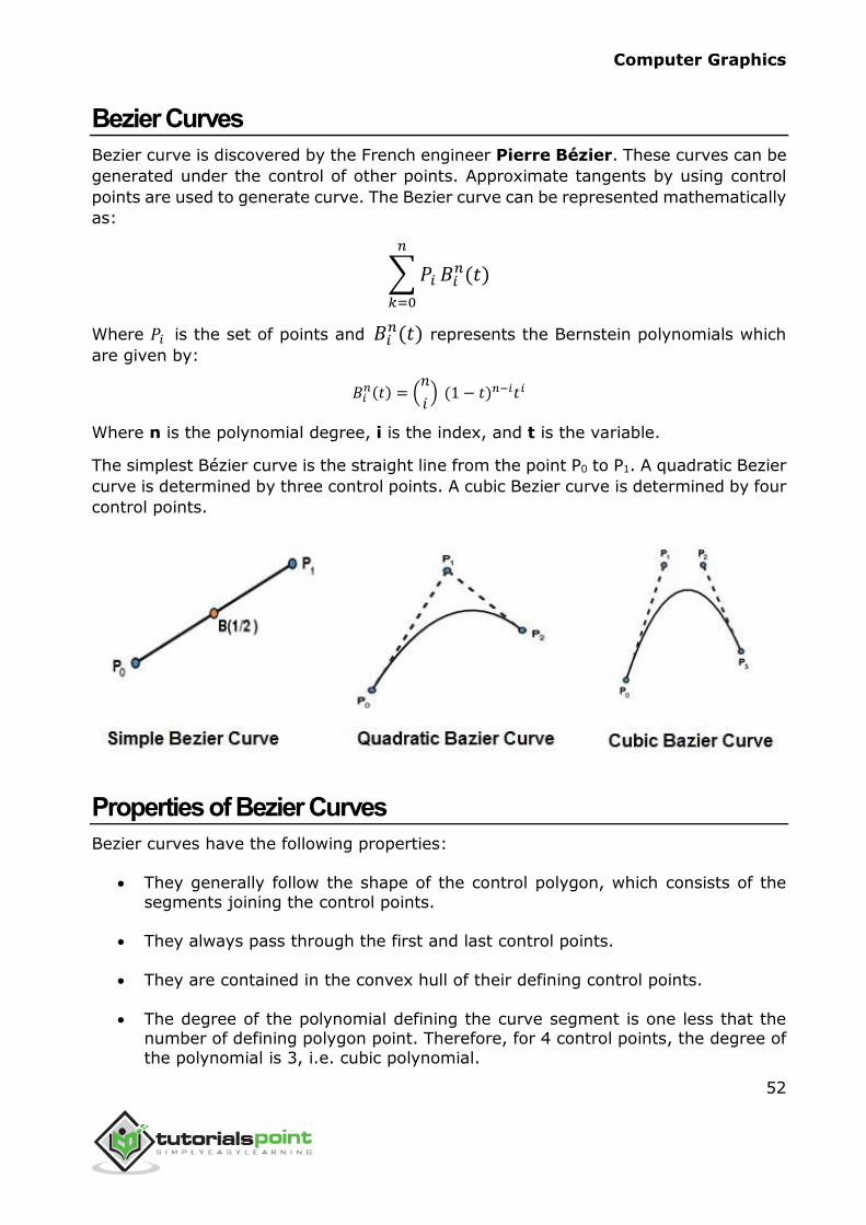
The simplest Bézier curve is the straight line from the point P0 to P1. A quadratic Bezier
curve is determined by three control points. A cubic Bezier curve is determined by four
control points.
Properties of Bezier Curves
Bezier curves have the following properties:
They generally follow the shape of the control polygon, which consists of the
segments joining the control points.
They always pass through the first and last control points.
They are contained in the convex hull of their defining control points.
The degree of the polynomial defining the curve segment is one less that the
number of defining polygon point. Therefore, for 4 control points, the degree of
the polynomial is 3, i.e. cubic polynomial.
Computer Graphics
53
A Bezier curve generally follows the shape of the defining polygon.
The direction of the tangent vector at the end points is same as that of the vector
determined by first and last segments.
The convex hull property for a Bezier curve ensures that the polynomial
smoothly follows the control points.
No straight line intersects a Bezier curve more times than it intersects its control polygon.
They are invariant under an affine transformation.
Bezier curves exhibit global control means moving a control point alters the shape of the whole curve.
A given Bezier curve can be subdivided at a point t=t0 into two Bezier segments
which join together at the point corresponding to the parameter value t=t0.
B-Spline Curves
The Bezier-curve produced by the Bernstein basis function has limited flexibility.
First, the number of specified polygon vertices fixes the order of the resulting polynomial which defines the curve.
The second limiting characteristic is that the value of the blending function is
nonzero for all parameter values over the entire curve.
The B-spline basis contains the Bernstein basis as the special case. The B-spline basis
is non-global.
A B-spline curve is defined as a linear combination of control points Pi and B-spline
basis function Ni, k (t) given by
C(t) = ∑ 𝑃𝑖𝑛𝑖=0 𝑁𝑖,𝑘(𝑡), n ≥ k - 1, t [ tk-1 , tn+1 ]
Where,
{𝑃𝑖: i=0, 1, 2….n} are the control points
k is the order of the polynomial segments of the B-spline curve. Order k means that the curve is made up of piecewise polynomial segments of degree k − 1,
the Ni,k(t) are the “normalized B-spline blending functions”. They are described
by the order k and by a non-decreasing sequence of real numbers normally called the “knot sequence”.
{ti : i = 0, ..., n + k}
Computer Graphics
54
The Ni, k functions are described as follows:
𝑁𝑖,1(𝑡) = {1, 𝑖𝑓 𝑢 [ 𝑡𝑖 , 𝑡𝑖+1 )
0, Otherwise
and if k > 1,
𝑁𝑖,𝑘(𝑡) = 𝑡 − 𝑡𝑖
𝑡𝑖+𝑘−1 − 𝑡𝑖 𝑁𝑖,𝑘−1(𝑡) +
𝑡𝑖+𝑘 − 𝑡
𝑡𝑖+𝑘 − 𝑡𝑖+1𝑁𝑖+1,𝑘−1(𝑡)
and
t [ tk-1,tn+1 )
Properties of B-spline Curve
B-spline curves have the following properties:
The sum of the B-spline basis functions for any parameter value is 1.
Each basis function is positive or zero for all parameter values.
Each basis function has precisely one maximum value, except for k=1.
The maximum order of the curve is equal to the number of vertices of defining polygon.
The degree of B-spline polynomial is independent on the number of vertices of
defining polygon.
B-spline allows the local control over the curve surface because each vertex
affects the shape of a curve only over a range of parameter values where its associated basis function is nonzero.
The curve exhibits the variation diminishing property.
The curve generally follows the shape of defining polygon.
Any affine transformation can be applied to the curve by applying it to the
vertices of defining polygon.
The curve line within the convex hull of its defining polygon.
Computer Graphics
55
Polygon Surfaces
Objects are represented as a collection of surfaces. 3D object representation is divided
into two categories.
Boundary Representations (B-reps): It describes a 3D object as a set of surfaces that separates the object interior from the environment.
Space–partitioning representations: It is used to describe interior
properties, by partitioning the spatial region containing an object into a set of small, non-overlapping, contiguous solids (usually cubes).
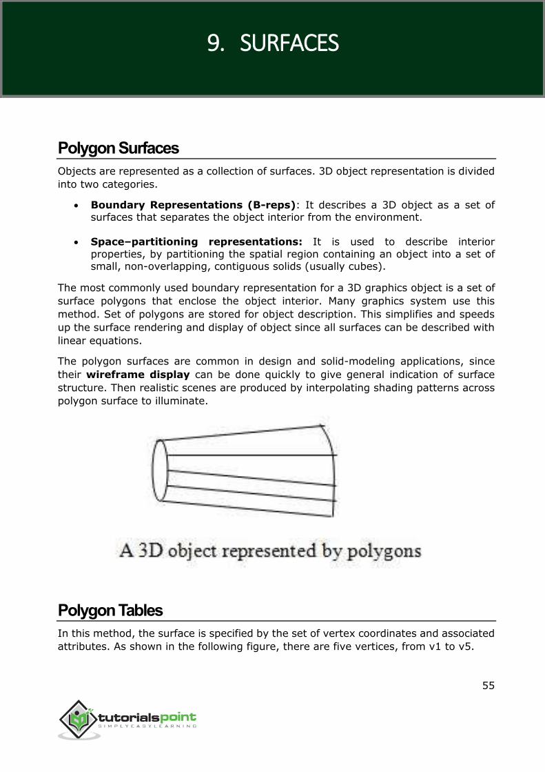
The most commonly used boundary representation for a 3D graphics object is a set of
surface polygons that enclose the object interior. Many graphics system use this
method. Set of polygons are stored for object description. This simplifies and speeds
up the surface rendering and display of object since all surfaces can be described with
linear equations.
The polygon surfaces are common in design and solid-modeling applications, since
their wireframe display can be done quickly to give general indication of surface
structure. Then realistic scenes are produced by interpolating shading patterns across
polygon surface to illuminate.
Polygon Tables
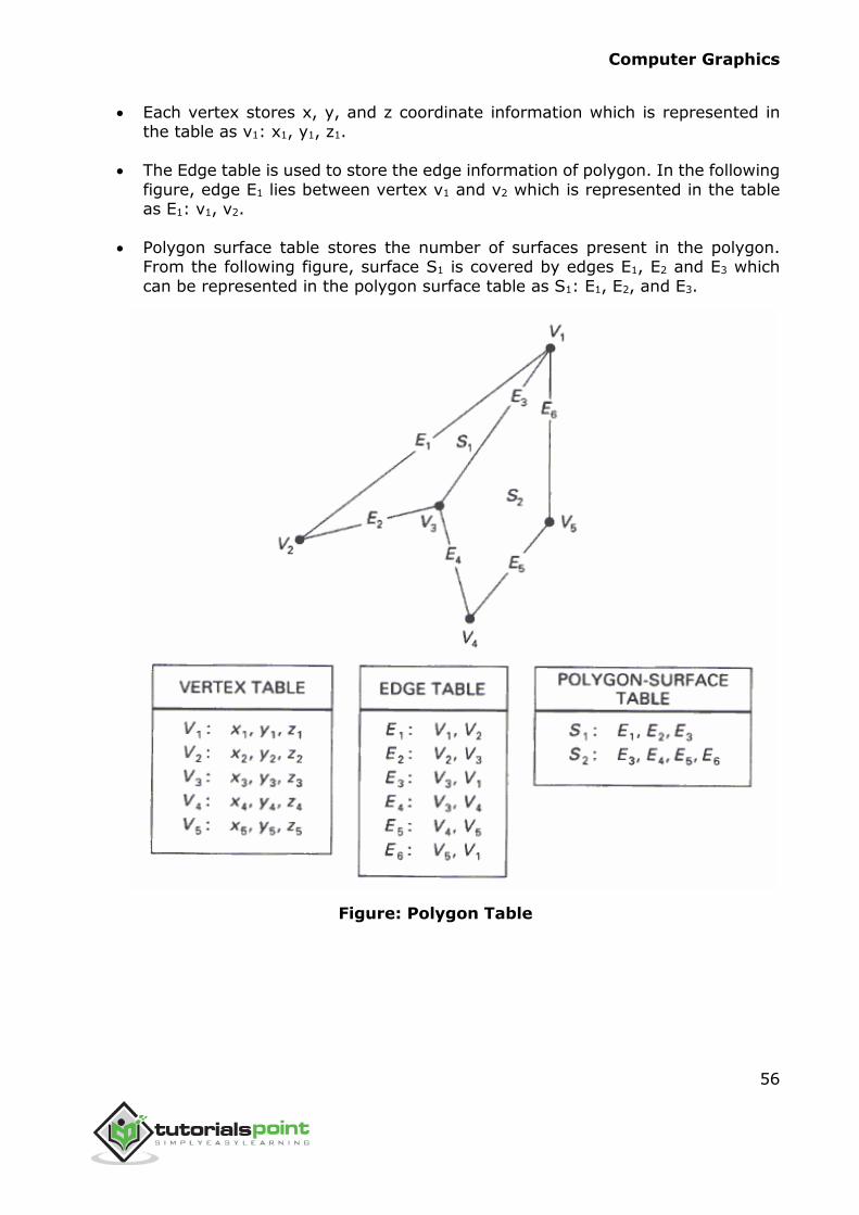
In this method, the surface is specified by the set of vertex coordinates and associated
attributes. As shown in the following figure, there are five vertices, from v1 to v5.
9. SURFACES
Computer Graphics
56
Each vertex stores x, y, and z coordinate information which is represented in the table as v1: x1, y1, z1.
The Edge table is used to store the edge information of polygon. In the following
figure, edge E1 lies between vertex v1 and v2 which is represented in the table as E1: v1, v2.
Polygon surface table stores the number of surfaces present in the polygon. From the following figure, surface S1 is covered by edges E1, E2 and E3 which
can be represented in the polygon surface table as S1: E1, E2, and E3.
Figure: Polygon Table
Computer Graphics
57
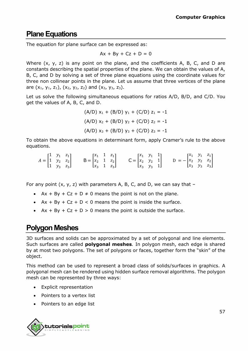
Plane Equations
The equation for plane surface can be expressed as:
Ax + By + Cz + D = 0
Where (x, y, z) is any point on the plane, and the coefficients A, B, C, and D are
constants describing the spatial properties of the plane. We can obtain the values of A,
B, C, and D by solving a set of three plane equations using the coordinate values for
three non collinear points in the plane. Let us assume that three vertices of the plane
are (x1, y1, z1), (x2, y2, z2) and (x3, y3, z3).
Let us solve the following simultaneous equations for ratios A/D, B/D, and C/D. You
get the values of A, B, C, and D.
(A/D) x1 + (B/D) y1 + (C/D) z1 = -1
(A/D) x2 + (B/D) y2 + (C/D) z2 = -1
(A/D) x3 + (B/D) y3 + (C/D) z3 = -1
To obtain the above equations in determinant form, apply Cramer’s rule to the above
equations.
𝐴 = [
1 𝑦1 𝑧1
1 𝑦2 𝑧2
1 𝑦3 𝑧3
] B = [
𝑥1 1 𝑧1
𝑥2 1 𝑧2
𝑥3 1 𝑧3
] C = [
𝑥1 𝑦1 1𝑥2 𝑦2 1𝑥3 𝑦3 1
] D = − [
𝑥1 𝑦1 𝑧1
𝑥2 𝑦2 𝑧2
𝑥3 𝑦3 𝑧3
]
For any point (x, y, z) with parameters A, B, C, and D, we can say that –
Ax + By + Cz + D ≠ 0 means the point is not on the plane.
Ax + By + Cz + D < 0 means the point is inside the surface.
Ax + By + Cz + D > 0 means the point is outside the surface.
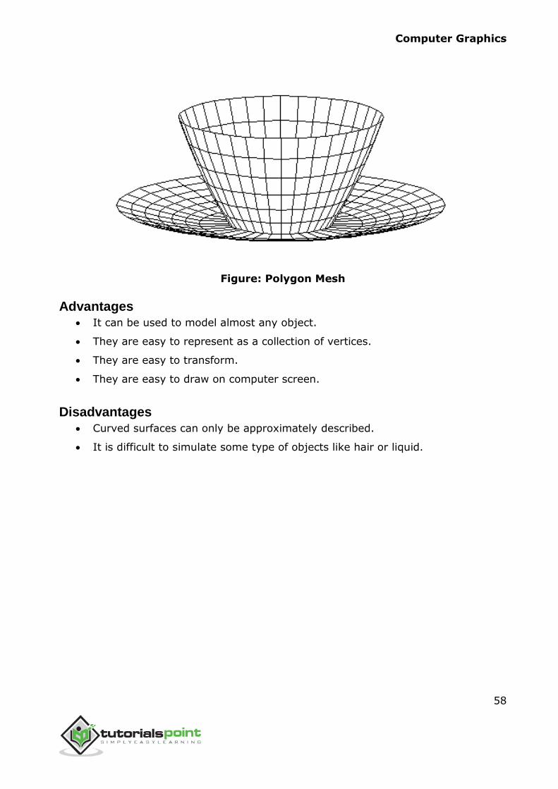
Polygon Meshes
3D surfaces and solids can be approximated by a set of polygonal and line elements.
Such surfaces are called polygonal meshes. In polygon mesh, each edge is shared
by at most two polygons. The set of polygons or faces, together form the “skin” of the
object.
This method can be used to represent a broad class of solids/surfaces in graphics. A
polygonal mesh can be rendered using hidden surface removal algorithms. The polygon
mesh can be represented by three ways:
Explicit representation
Pointers to a vertex list
Pointers to an edge list
Computer Graphics
58
Figure: Polygon Mesh
Advantages It can be used to model almost any object.
They are easy to represent as a collection of vertices.
They are easy to transform.
They are easy to draw on computer screen.
Disadvantages
Curved surfaces can only be approximately described.
It is difficult to simulate some type of objects like hair or liquid.
Computer Graphics
59
When we view a picture containing non-transparent objects and surfaces, then we
cannot see those objects from view which are behind from objects closer to eye. We
must remove these hidden surfaces to get a realistic screen image. The identification
and removal of these surfaces is called Hidden-surface problem.
There are two approaches for removing hidden surface problems: Object-Space
method and Image-space method. The Object-space method is implemented in
physical coordinate system and image-space method is implemented in screen
coordinate system.
When we want to display a 3D object on a 2D screen, we need to identify those parts
of a screen that are visible from a chosen viewing position.
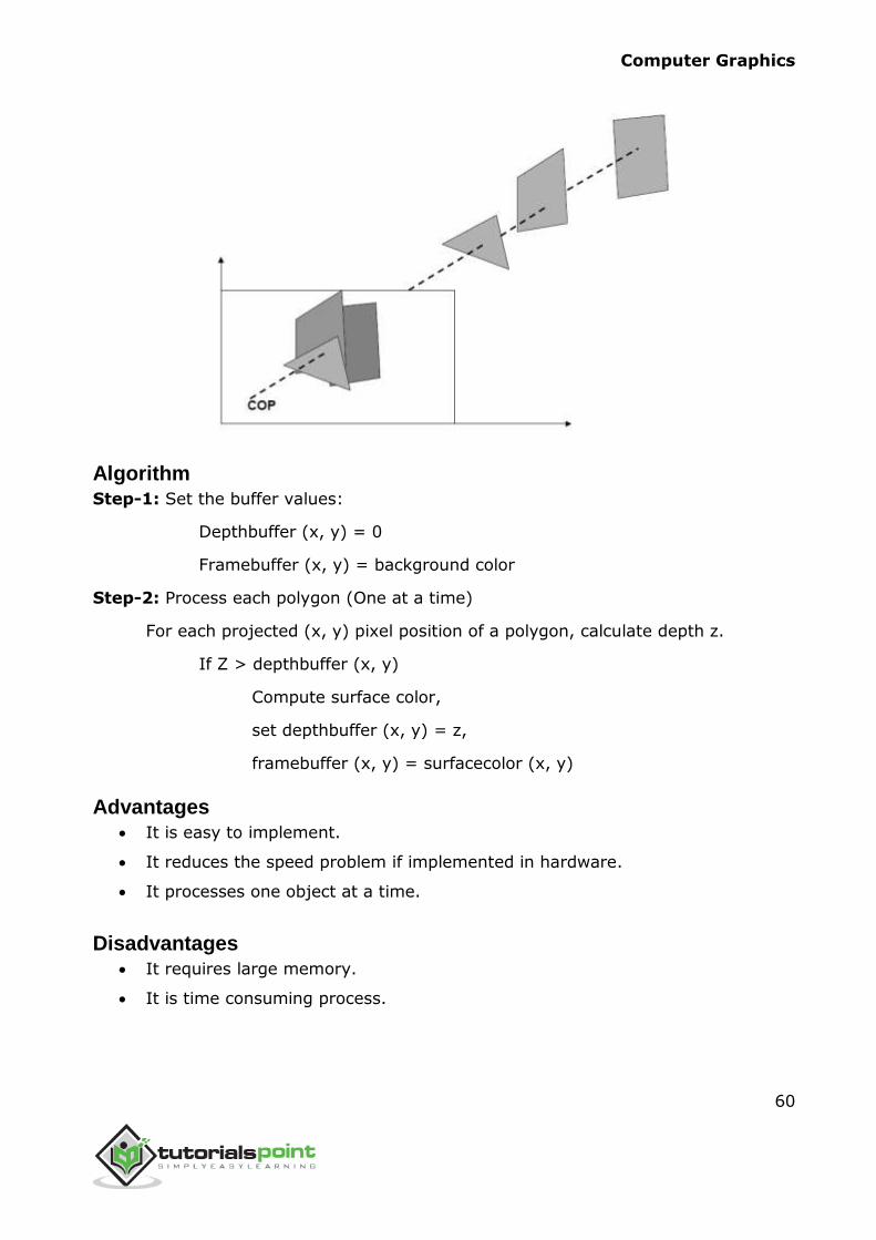
Depth Buffer (Z-Buffer) Method
This method is developed by Cutmull. It is an image-space approach. The basic idea is
to test the Z-depth of each surface to determine the closest (visible) surface.
In this method each surface is processed separately one pixel position at a time across
the surface. The depth values for a pixel are compared and the closest (smallest z)
surface determines the color to be displayed in the frame buffer.
It is applied very efficiently on surfaces of polygon. Surfaces can be processed in any
order. To override the closer polygons from the far ones, two buffers named frame
buffer and depth buffer, are used.
Depth buffer is used to store depth values for (x, y) position, as surfaces are
processed (0 ≤ depth ≤ 1).
The frame buffer is used to store the intensity value of color value at each position
(x, y).
The z-coordinates are usually normalized to the range [0, 1]. The 0 value for z-
coordinate indicates back clipping pane and 1 value for z-coordinates indicates front
clipping pane.
10. VISIBLE SURFACE DETECTION
Computer Graphics
60
Algorithm Step-1: Set the buffer values:
Depthbuffer (x, y) = 0
Framebuffer (x, y) = background color
Step-2: Process each polygon (One at a time)
For each projected (x, y) pixel position of a polygon, calculate depth z.
If Z > depthbuffer (x, y)
Compute surface color,
set depthbuffer (x, y) = z,
framebuffer (x, y) = surfacecolor (x, y)
Advantages It is easy to implement.
It reduces the speed problem if implemented in hardware.
It processes one object at a time.
Disadvantages
It requires large memory.
It is time consuming process.
Computer Graphics
61
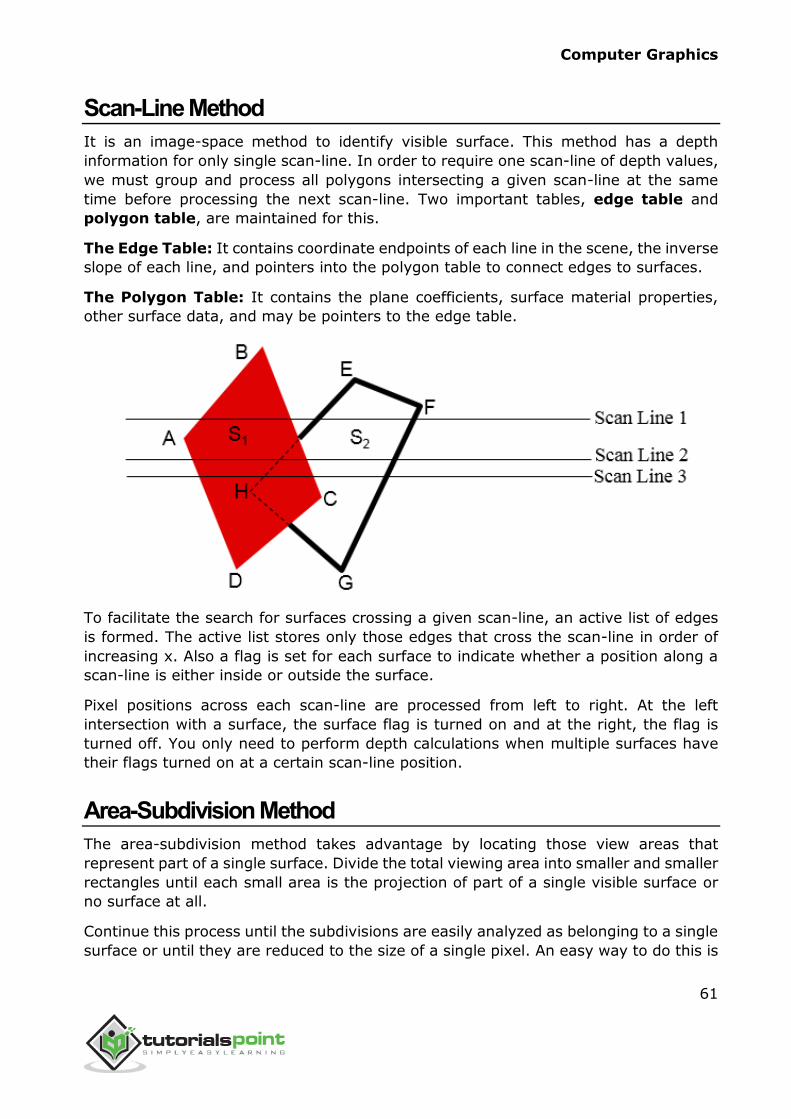
Scan-Line Method
It is an image-space method to identify visible surface. This method has a depth
information for only single scan-line. In order to require one scan-line of depth values,
we must group and process all polygons intersecting a given scan-line at the same
time before processing the next scan-line. Two important tables, edge table and
polygon table, are maintained for this.
The Edge Table: It contains coordinate endpoints of each line in the scene, the inverse
slope of each line, and pointers into the polygon table to connect edges to surfaces.
The Polygon Table: It contains the plane coefficients, surface material properties,
other surface data, and may be pointers to the edge table.
To facilitate the search for surfaces crossing a given scan-line, an active list of edges
is formed. The active list stores only those edges that cross the scan-line in order of
increasing x. Also a flag is set for each surface to indicate whether a position along a
scan-line is either inside or outside the surface.
Pixel positions across each scan-line are processed from left to right. At the left
intersection with a surface, the surface flag is turned on and at the right, the flag is
turned off. You only need to perform depth calculations when multiple surfaces have
their flags turned on at a certain scan-line position.
Area-Subdivision Method
The area-subdivision method takes advantage by locating those view areas that
represent part of a single surface. Divide the total viewing area into smaller and smaller
rectangles until each small area is the projection of part of a single visible surface or
no surface at all.
Continue this process until the subdivisions are easily analyzed as belonging to a single
surface or until they are reduced to the size of a single pixel. An easy way to do this is
Computer Graphics
62
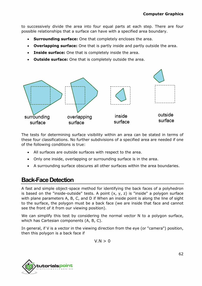
to successively divide the area into four equal parts at each step. There are four
possible relationships that a surface can have with a specified area boundary.
Surrounding surface: One that completely encloses the area.
Overlapping surface: One that is partly inside and partly outside the area.
Inside surface: One that is completely inside the area.
Outside surface: One that is completely outside the area.
The tests for determining surface visibility within an area can be stated in terms of
these four classifications. No further subdivisions of a specified area are needed if one
of the following conditions is true:
All surfaces are outside surfaces with respect to the area.
Only one inside, overlapping or surrounding surface is in the area.
A surrounding surface obscures all other surfaces within the area boundaries.
Back-Face Detection
A fast and simple object-space method for identifying the back faces of a polyhedron
is based on the "inside-outside" tests. A point (x, y, z) is "inside" a polygon surface
with plane parameters A, B, C, and D if When an inside point is along the line of sight
to the surface, the polygon must be a back face (we are inside that face and cannot
see the front of it from our viewing position).
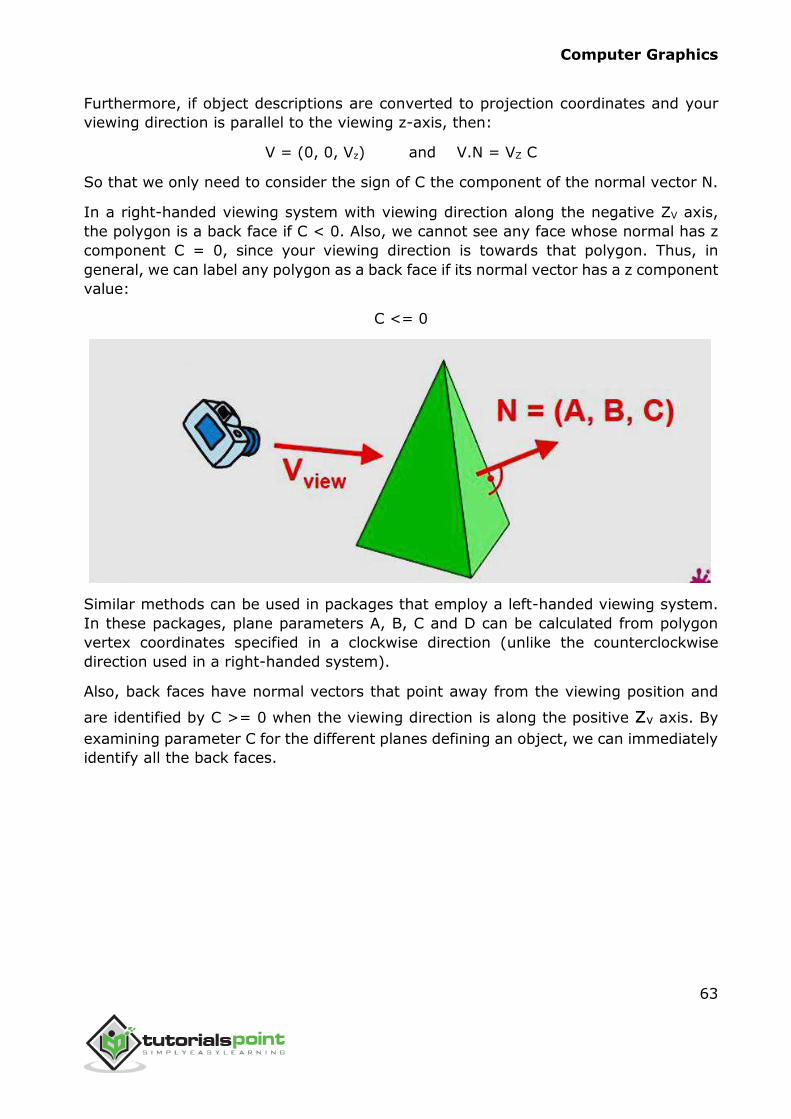
We can simplify this test by considering the normal vector N to a polygon surface,
which has Cartesian components (A, B, C).
In general, if V is a vector in the viewing direction from the eye (or "camera") position,
then this polygon is a back face if
V.N > 0
Computer Graphics
63
Furthermore, if object descriptions are converted to projection coordinates and your
viewing direction is parallel to the viewing z-axis, then:
V = (0, 0, Vz) and V.N = VZ C
So that we only need to consider the sign of C the component of the normal vector N.
In a right-handed viewing system with viewing direction along the negative ZV axis,
the polygon is a back face if C < 0. Also, we cannot see any face whose normal has z
component C = 0, since your viewing direction is towards that polygon. Thus, in
general, we can label any polygon as a back face if its normal vector has a z component
value:
C <= 0
Similar methods can be used in packages that employ a left-handed viewing system.
In these packages, plane parameters A, B, C and D can be calculated from polygon
vertex coordinates specified in a clockwise direction (unlike the counterclockwise
direction used in a right-handed system).
Also, back faces have normal vectors that point away from the viewing position and
are identified by C >= 0 when the viewing direction is along the positive zv axis. By
examining parameter C for the different planes defining an object, we can immediately
identify all the back faces.
Computer Graphics
64
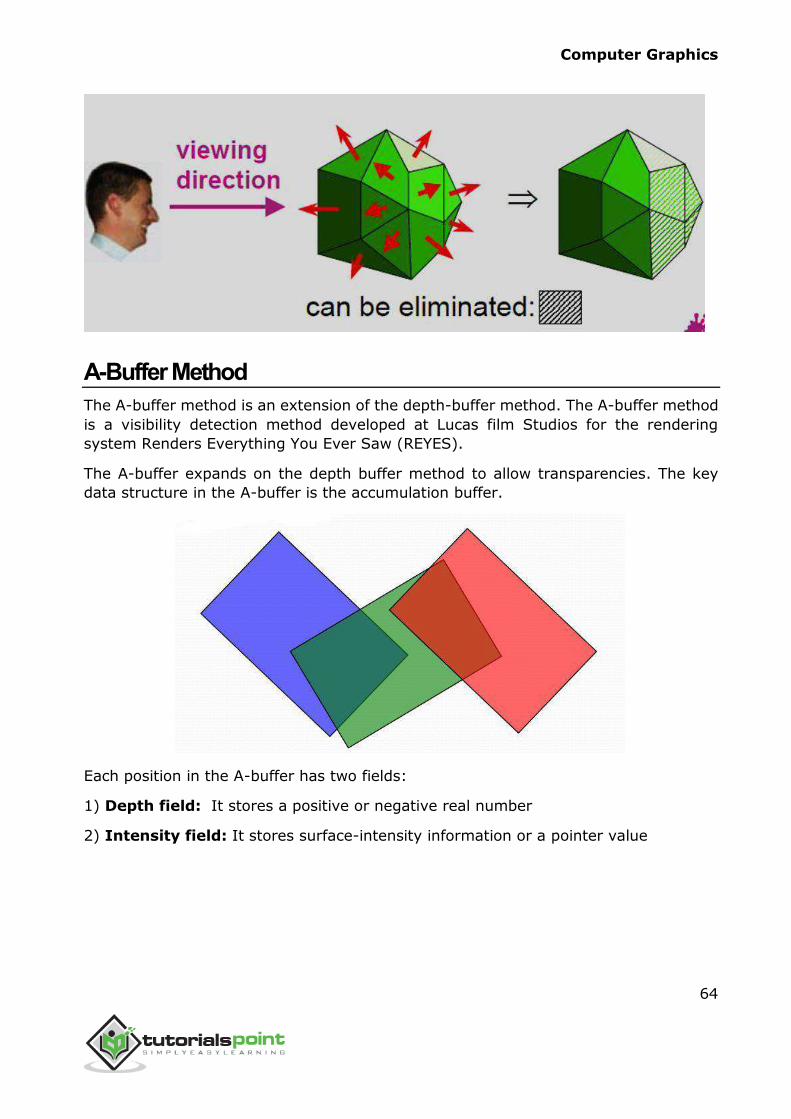
A-Buffer Method
The A-buffer method is an extension of the depth-buffer method. The A-buffer method
is a visibility detection method developed at Lucas film Studios for the rendering
system Renders Everything You Ever Saw (REYES).
The A-buffer expands on the depth buffer method to allow transparencies. The key
data structure in the A-buffer is the accumulation buffer.
Each position in the A-buffer has two fields:
1) Depth field: It stores a positive or negative real number
2) Intensity field: It stores surface-intensity information or a pointer value
Computer Graphics
65
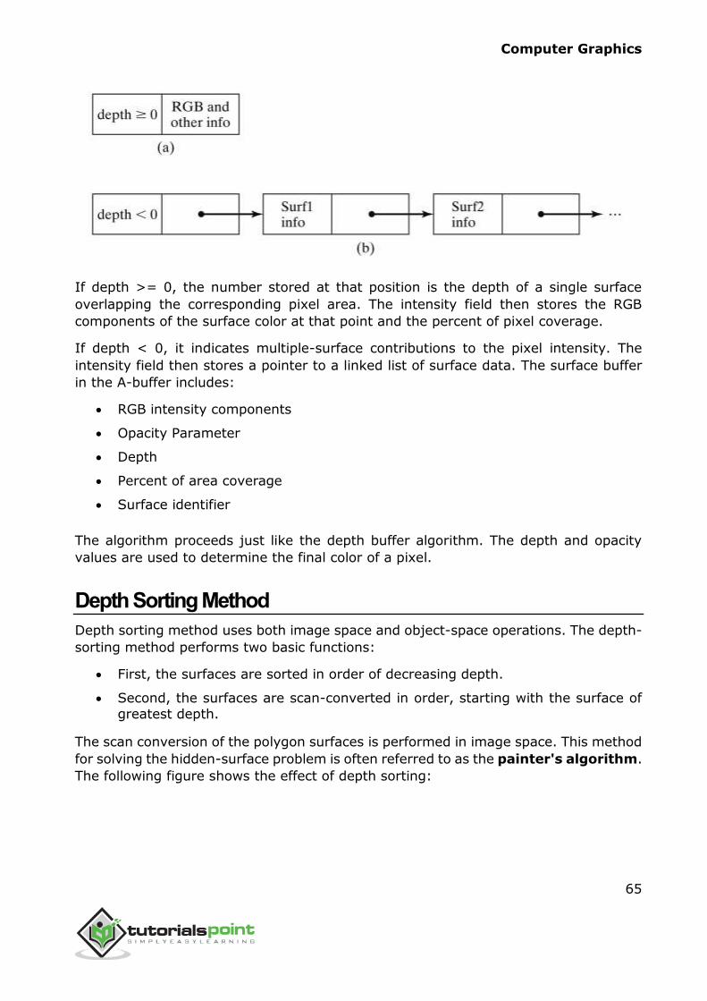
If depth >= 0, the number stored at that position is the depth of a single surface
overlapping the corresponding pixel area. The intensity field then stores the RGB
components of the surface color at that point and the percent of pixel coverage.
If depth < 0, it indicates multiple-surface contributions to the pixel intensity. The
intensity field then stores a pointer to a linked list of surface data. The surface buffer
in the A-buffer includes:
RGB intensity components
Opacity Parameter
Depth
Percent of area coverage
Surface identifier
The algorithm proceeds just like the depth buffer algorithm. The depth and opacity
values are used to determine the final color of a pixel.
Depth Sorting Method
Depth sorting method uses both image space and object-space operations. The depth-
sorting method performs two basic functions:
First, the surfaces are sorted in order of decreasing depth.
Second, the surfaces are scan-converted in order, starting with the surface of
greatest depth.
The scan conversion of the polygon surfaces is performed in image space. This method
for solving the hidden-surface problem is often referred to as the painter's algorithm.
The following figure shows the effect of depth sorting:
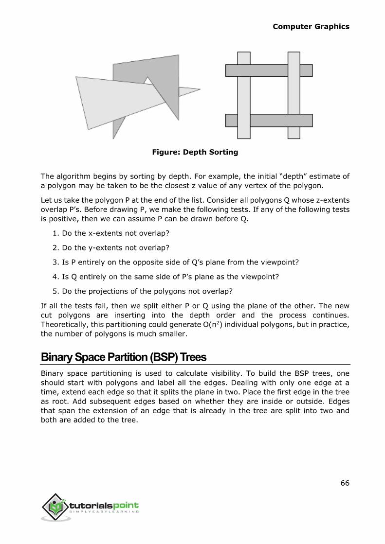
Computer Graphics
66
Figure: Depth Sorting
The algorithm begins by sorting by depth. For example, the initial “depth” estimate of
a polygon may be taken to be the closest z value of any vertex of the polygon.
Let us take the polygon P at the end of the list. Consider all polygons Q whose z-extents
overlap P’s. Before drawing P, we make the following tests. If any of the following tests
is positive, then we can assume P can be drawn before Q.
1. Do the x-extents not overlap?
2. Do the y-extents not overlap?
3. Is P entirely on the opposite side of Q’s plane from the viewpoint?
4. Is Q entirely on the same side of P’s plane as the viewpoint?
5. Do the projections of the polygons not overlap?
If all the tests fail, then we split either P or Q using the plane of the other. The new
cut polygons are inserting into the depth order and the process continues.
Theoretically, this partitioning could generate O(n2) individual polygons, but in practice,
the number of polygons is much smaller.
Binary Space Partition (BSP) Trees
Binary space partitioning is used to calculate visibility. To build the BSP trees, one
should start with polygons and label all the edges. Dealing with only one edge at a
time, extend each edge so that it splits the plane in two. Place the first edge in the tree
as root. Add subsequent edges based on whether they are inside or outside. Edges
that span the extension of an edge that is already in the tree are split into two and
both are added to the tree.
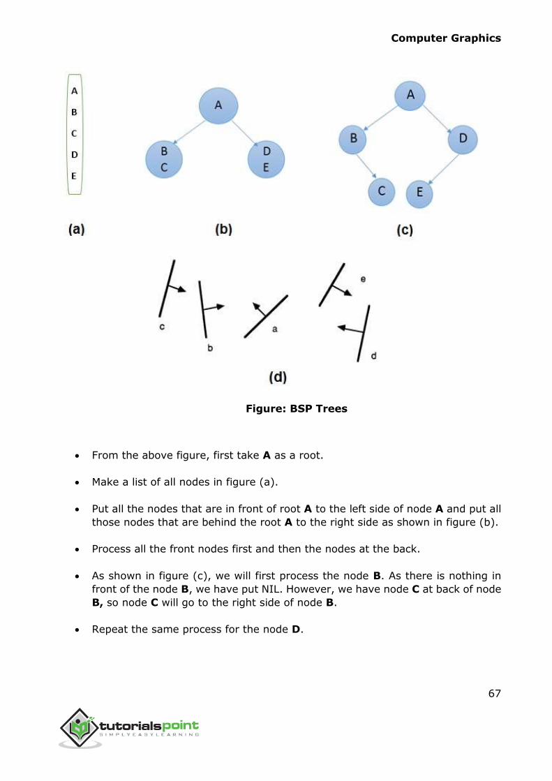
Computer Graphics
67
Figure: BSP Trees
From the above figure, first take A as a root.
Make a list of all nodes in figure (a).
Put all the nodes that are in front of root A to the left side of node A and put all
those nodes that are behind the root A to the right side as shown in figure (b).
Process all the front nodes first and then the nodes at the back.
As shown in figure (c), we will first process the node B. As there is nothing in
front of the node B, we have put NIL. However, we have node C at back of node
B, so node C will go to the right side of node B.
Repeat the same process for the node D.
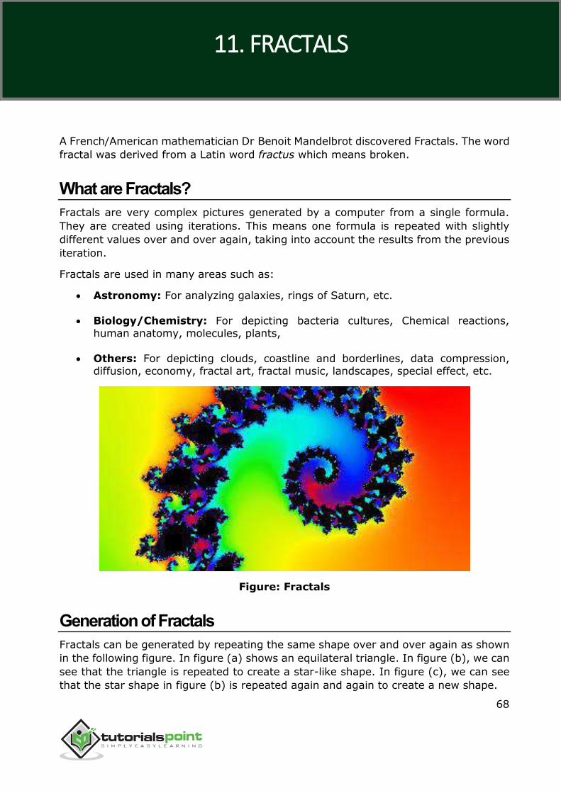
Computer Graphics
68
A French/American mathematician Dr Benoit Mandelbrot discovered Fractals. The word
fractal was derived from a Latin word fractus which means broken.
What are Fractals?
Fractals are very complex pictures generated by a computer from a single formula.
They are created using iterations. This means one formula is repeated with slightly
different values over and over again, taking into account the results from the previous
iteration.
Fractals are used in many areas such as:
Astronomy: For analyzing galaxies, rings of Saturn, etc.
Biology/Chemistry: For depicting bacteria cultures, Chemical reactions, human anatomy, molecules, plants,
Others: For depicting clouds, coastline and borderlines, data compression,
diffusion, economy, fractal art, fractal music, landscapes, special effect, etc.
Figure: Fractals
Generation of Fractals
Fractals can be generated by repeating the same shape over and over again as shown
in the following figure. In figure (a) shows an equilateral triangle. In figure (b), we can
see that the triangle is repeated to create a star-like shape. In figure (c), we can see
that the star shape in figure (b) is repeated again and again to create a new shape.
11. FRACTALS
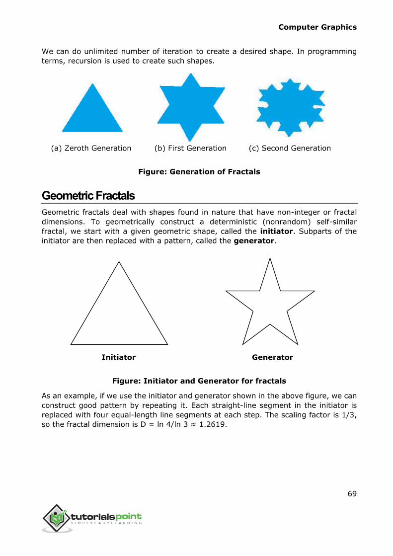
Computer Graphics
69
We can do unlimited number of iteration to create a desired shape. In programming
terms, recursion is used to create such shapes.
(a) Zeroth Generation (b) First Generation (c) Second Generation
Figure: Generation of Fractals
Geometric Fractals
Geometric fractals deal with shapes found in nature that have non-integer or fractal
dimensions. To geometrically construct a deterministic (nonrandom) self-similar
fractal, we start with a given geometric shape, called the initiator. Subparts of the
initiator are then replaced with a pattern, called the generator.
Initiator
Generator
Figure: Initiator and Generator for fractals
As an example, if we use the initiator and generator shown in the above figure, we can
construct good pattern by repeating it. Each straight-line segment in the initiator is
replaced with four equal-length line segments at each step. The scaling factor is 1/3,
so the fractal dimension is D = ln 4/ln 3 ≈ 1.2619.
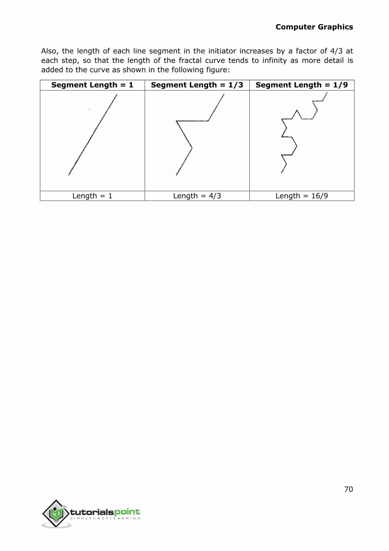
Computer Graphics
70
Also, the length of each line segment in the initiator increases by a factor of 4/3 at
each step, so that the length of the fractal curve tends to infinity as more detail is
added to the curve as shown in the following figure:
Segment Length = 1 Segment Length = 1/3 Segment Length = 1/9
Length = 1 Length = 4/3 Length = 16/9
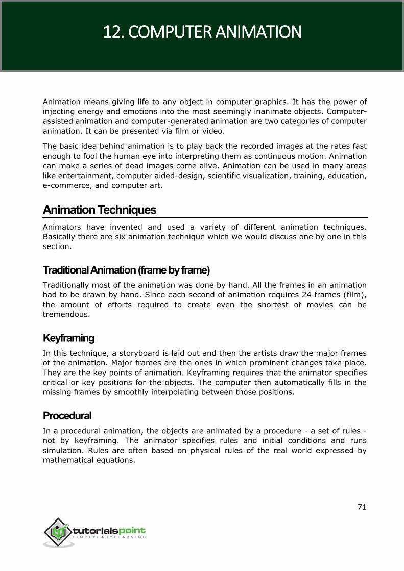
Computer Graphics
71
Animation means giving life to any object in computer graphics. It has the power of
injecting energy and emotions into the most seemingly inanimate objects. Computer-
assisted animation and computer-generated animation are two categories of computer
animation. It can be presented via film or video.
The basic idea behind animation is to play back the recorded images at the rates fast
enough to fool the human eye into interpreting them as continuous motion. Animation
can make a series of dead images come alive. Animation can be used in many areas
like entertainment, computer aided-design, scientific visualization, training, education,
e-commerce, and computer art.
Animation Techniques
Animators have invented and used a variety of different animation techniques.
Basically there are six animation technique which we would discuss one by one in this
section.
Traditional Animation (frame by frame)
Traditionally most of the animation was done by hand. All the frames in an animation
had to be drawn by hand. Since each second of animation requires 24 frames (film),
the amount of efforts required to create even the shortest of movies can be
tremendous.
Keyframing
In this technique, a storyboard is laid out and then the artists draw the major frames
of the animation. Major frames are the ones in which prominent changes take place.
They are the key points of animation. Keyframing requires that the animator specifies
critical or key positions for the objects. The computer then automatically fills in the
missing frames by smoothly interpolating between those positions.
Procedural
In a procedural animation, the objects are animated by a procedure - a set of rules -
not by keyframing. The animator specifies rules and initial conditions and runs
simulation. Rules are often based on physical rules of the real world expressed by
mathematical equations.
12. COMPUTER ANIMATION
Computer Graphics
72
Behavioral
In behavioral animation, an autonomous character determines its own actions, at least
to a certain extent. This gives the character some ability to improvise, and frees the
animator from the need to specify each detail of every character's motion.
Performance Based (Motion Capture)
Another technique is Motion Capture, in which magnetic or vision-based sensors record
the actions of a human or animal object in three dimensions. A computer then uses
these data to animate the object.
This technology has enabled a number of famous athletes to supply the actions for
characters in sports video games. Motion capture is pretty popular with the animators
mainly because some of the commonplace human actions can be captured with relative
ease. However, there can be serious discrepancies between the shapes or dimensions
of the subject and the graphical character and this may lead to problems of exact
execution.
Physically Based (Dynamics)
Unlike key framing and motion picture, simulation uses the laws of physics to generate
motion of pictures and other objects. Simulations can be easily used to produce slightly
different sequences while maintaining physical realism. Secondly, real-time simulations
allow a higher degree of interactivity where the real person can maneuver the actions
of the simulated character.
In contrast the applications based on key-framing and motion select and modify
motions form a pre-computed library of motions. One drawback that simulation suffers
from is the expertise and time required to handcraft the appropriate controls systems.
Key Framing
A keyframe is a frame where we define changes in animation. Every frame is a
keyframe when we create frame by frame animation. When someone creates a 3D
animation on a computer, they usually don’t specify the exact position of any given
object on every single frame. They create keyframes.
Keyframes are important frames during which an object changes its size, direction,
shape or other properties. The computer then figures out all the in-between frames
and saves an extreme amount of time for the animator. The following illustrations
depict the frames drawn by user and the frames generated by computer.
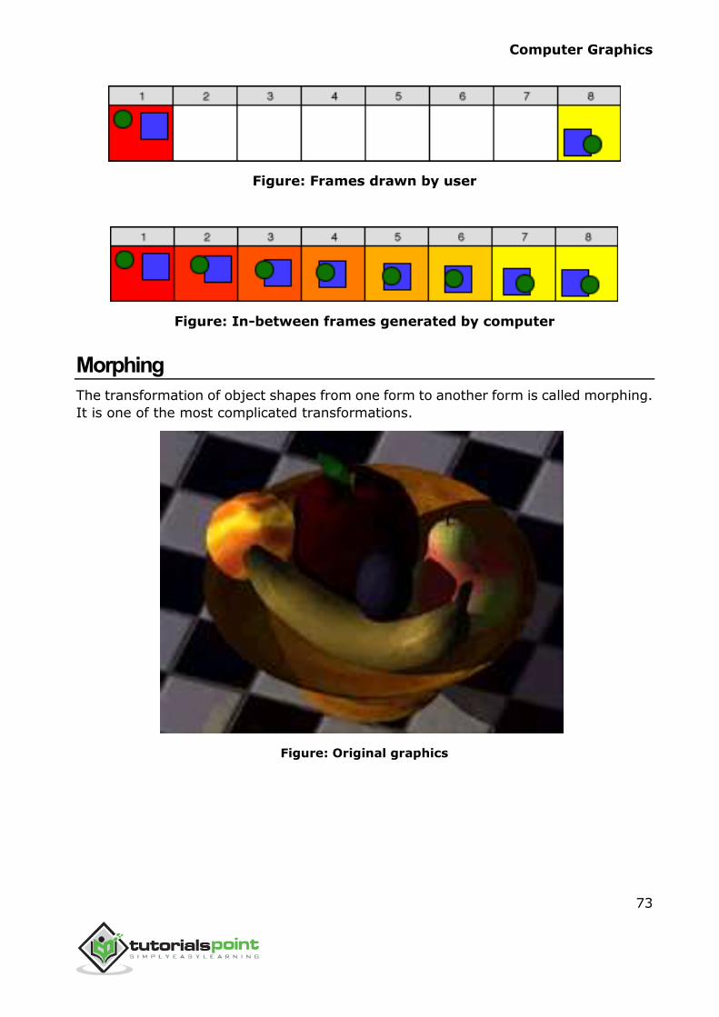
Computer Graphics
73
Figure: Frames drawn by user
Figure: In-between frames generated by computer
Morphing
The transformation of object shapes from one form to another form is called morphing.
It is one of the most complicated transformations.
Figure: Original graphics
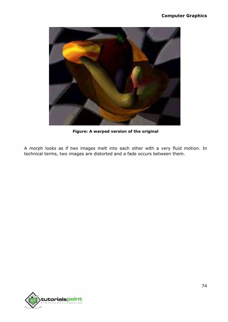
Computer Graphics
74
Figure: A warped version of the original
A morph looks as if two images melt into each other with a very fluid motion. In
technical terms, two images are distorted and a fade occurs between them.