Embed Size (px)
Citation preview
Computer VisionLocal Invariant Features
Mehdi [email protected]
SLIDES have been prepared by:Dr. Ghassabi
2
Outline• Why do we care about matching features?• Problem Statement
– Properties of features– Types of invariance
• Introduction to feature matching– Matching using invariant descriptors
• Feature Detection– Corner Detection
» Moravec, harris» Harris properties (rotation, intensity, scale invariance)
– Low’s key point
• Feature description– SIFT (Scale Invariant Feature Transform)– SIFT Extensions: PCA-SIFT, GLoH ,SPIN image, RIFT,
• Feature matching
• Applications (examples)• Future Works • Conclusion
Outline
Motivation
Problems statement
How we solve it
Future Work
Reference
3
Motivation
• Why do we care about matching features?– image stitching, – object recognition, – Indexing and database retrieval,– Motion tracking– … Others
Outline
Motivation
Problems statement
How we solve it
Future Work
Reference
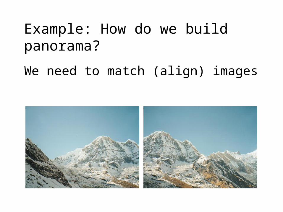
Example: How do we build panorama?
We need to match (align) images
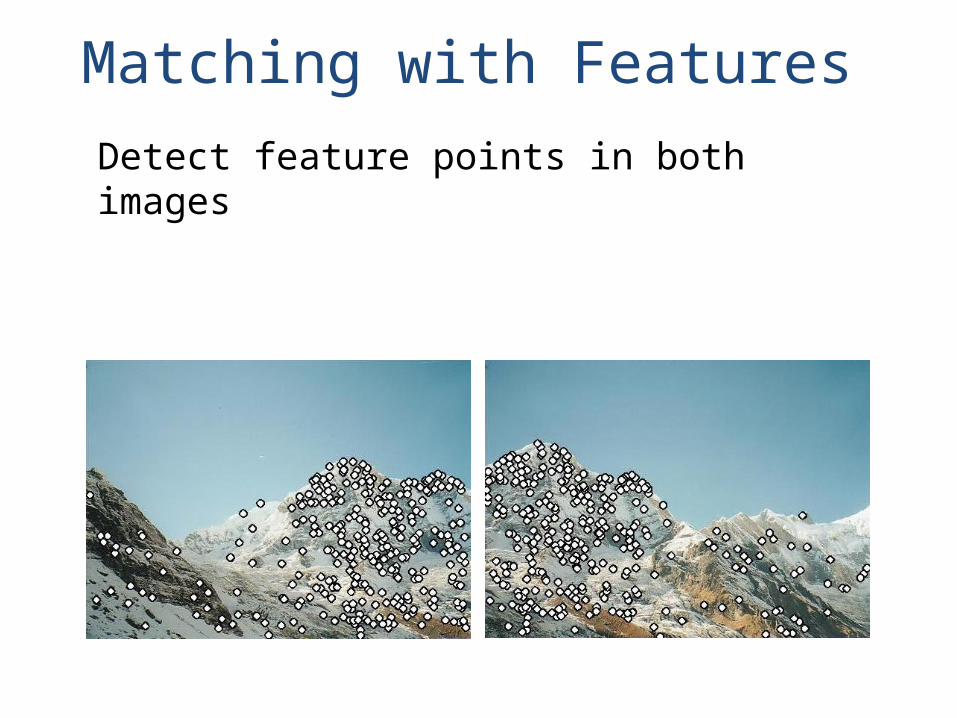
Matching with FeaturesDetect feature points in both images
6
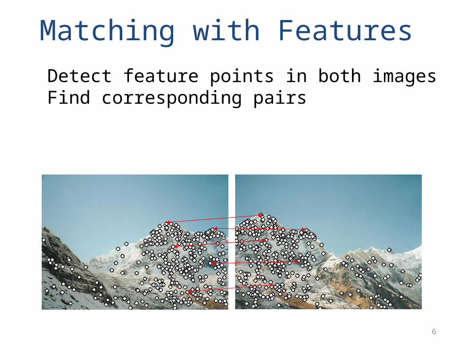
Matching with FeaturesDetect feature points in both imagesFind corresponding pairs
7
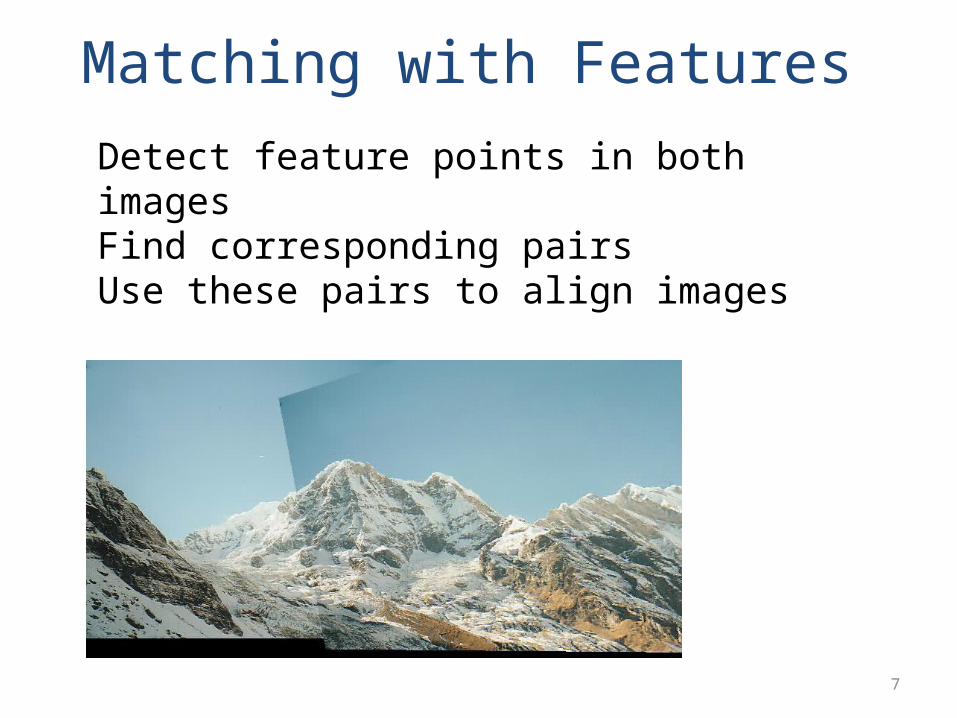
Matching with FeaturesDetect feature points in both imagesFind corresponding pairsUse these pairs to align images

8
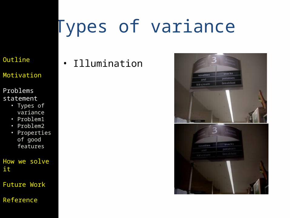
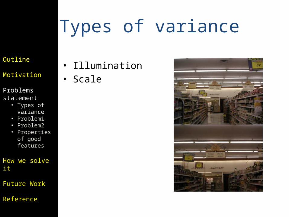
• Types of variance– Illumination– Scale– Rotation– Affine– Full Perspective
• Problems statements• Properties of good features
Outline
Motivation
Problems statement
How we solve it
Future Work
Reference
9
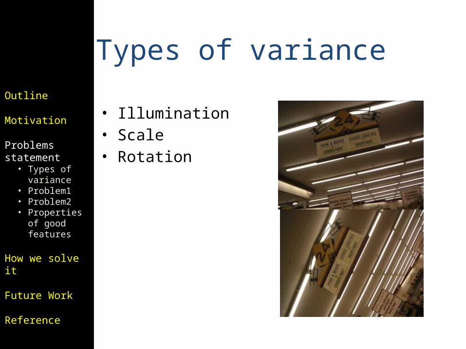
Types of variance
• IlluminationOutline
Motivation
Problems statement
• Types of variance
• Problem1• Problem2• Properties
of good features
How we solve it
Future Work
Reference
10
Types of variance
• Illumination• Scale
Outline
Motivation
Problems statement
• Types of variance
• Problem1• Problem2• Properties
of good features
How we solve it
Future Work
Reference
11
Types of variance
• Illumination• Scale• Rotation
Outline
Motivation
Problems statement
• Types of variance
• Problem1• Problem2• Properties
of good features
How we solve it
Future Work
Reference
12
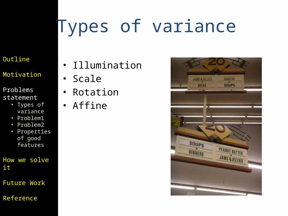
Types of variance
• Illumination• Scale• Rotation• Affine
Outline
Motivation
Problems statement
• Types of variance
• Problem1• Problem2• Properties
of good features
How we solve it
Future Work
Reference
13
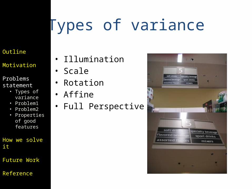
Types of variance
• Illumination• Scale• Rotation• Affine• Full Perspective
Outline
Motivation
Problems statement
• Types of variance
• Problem1• Problem2• Properties
of good features
How we solve it
Future Work
Reference
14
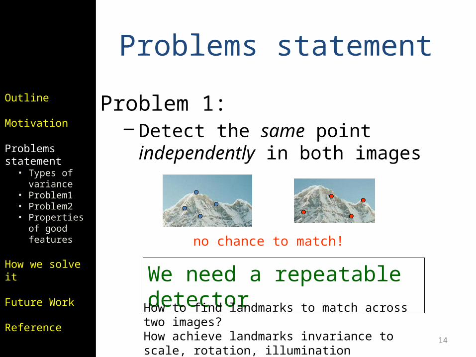
Problems statement
Problem 1:– Detect the same point independently in
both images
no chance to match!
We need a repeatable detectorHow to find landmarks to match across two images?How achieve landmarks invariance to scale, rotation, illumination distortions?
Outline
Motivation
Problems statement
• Types of variance
• Problem1• Problem2• Properties
of good features
How we solve it
Future Work
Reference
15
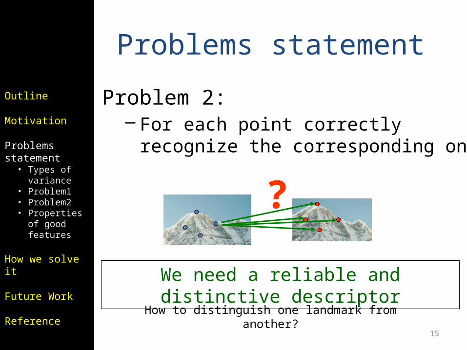
Problems statement
Problem 2:– For each point correctly recognize the
corresponding one
?
We need a reliable and distinctive descriptor
How to distinguish one landmark from another?
Outline
Motivation
Problems statement
• Types of variance
• Problem1• Problem2• Properties
of good features
How we solve it
Future Work
Reference
16
Properties of features
• Distinctiveness• Invariance
– Invariance to illumination, scale, Rotation, Affine, full perspective
Good features should be robust to all sorts of distortions that can occur
between images.
Outline
Motivation
Problems statement
• Types of variance
• Problem1• Problem2• Properties
of good features
How we solve it
Future Work
Reference
17
Methods using invariant descriptors
• Methods using invariant descriptors Invariance to: transformation change in illumination image noise Distinctiveness
• Local features– Feature Detector– Feature descriptor– Feature-matching
Outline
Motivation
Problems statement
How we solve it
• Methods of Feature matching
• Invariant descriptors
Future Work
Reference
18
Methods using invariant descriptors
• Local features– Feature Detector
• Point detector– Corner detectors
» Moravec, harris, SUSAN, Trajkovic operators– Low’s key point
• Region detector– Harris-Laplase, Harris affine, Hessian affine, edge-
based, Intensity-based, salient region detectors
– Feature descriptor– Feature-matching
Outline
Motivation
Problems statement
How we solve it
• Methods of Feature matching
• Invariant descriptors
Future Work
Reference
19
Methods using invariant descriptors
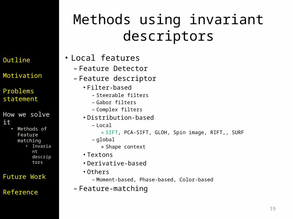
• Local features– Feature Detector– Feature descriptor
• Filter-based– Steerable filters– Gabor filters– Complex filters
• Distribution-based– Local
» SIFT, PCA-SIFT, GLOH, Spin image, RIFT,, SURF– global
» Shape context
• Textons• Derivative-based• Others
– Moment-based, Phase-based, Color-based
– Feature-matching
Outline
Motivation
Problems statement
How we solve it
• Methods of Feature matching
• Invariant descriptors
Future Work
Reference
20
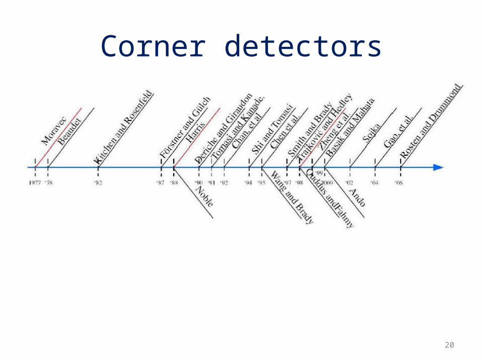
Corner detectors
21
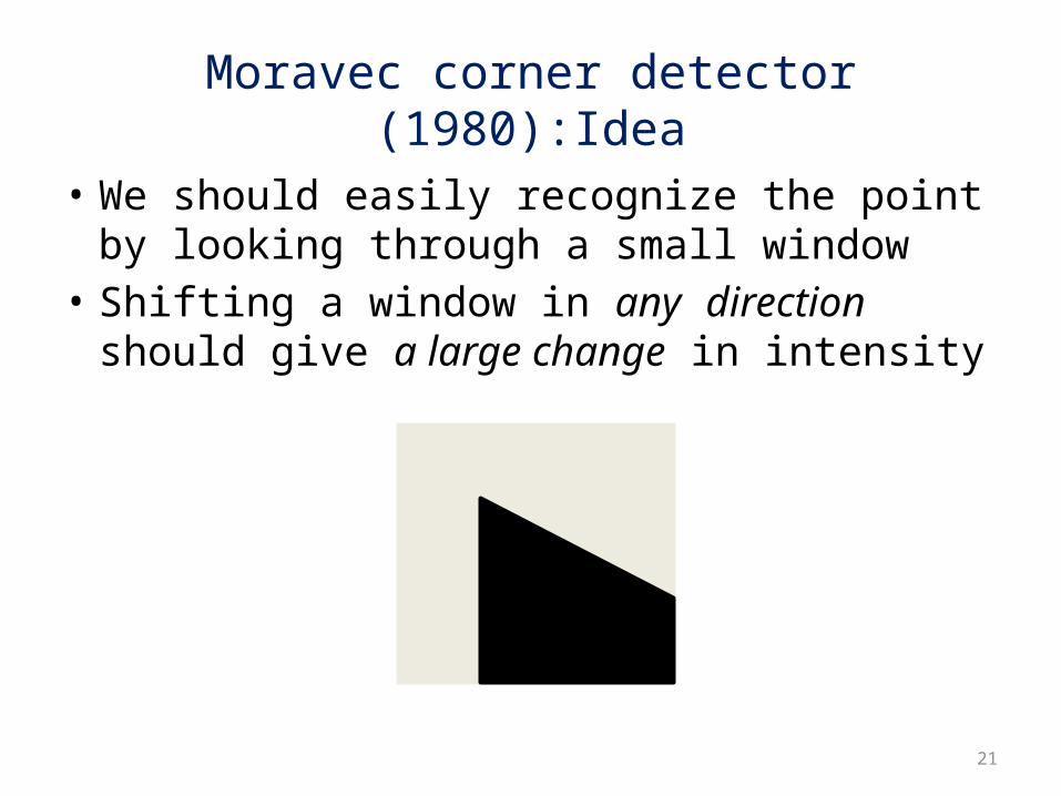
Moravec corner detector (1980):Idea
• We should easily recognize the point by looking through a small window
• Shifting a window in any direction should give a large change in intensity
22
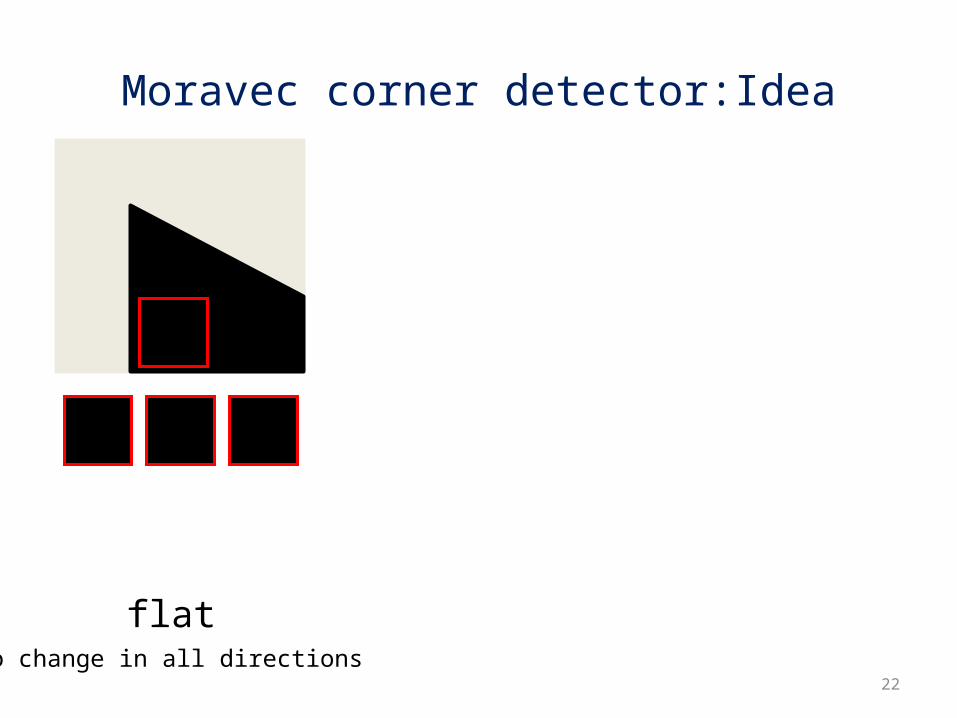
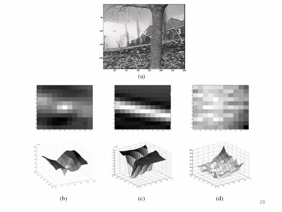
Moravec corner detector:Idea
flatno change in all directions
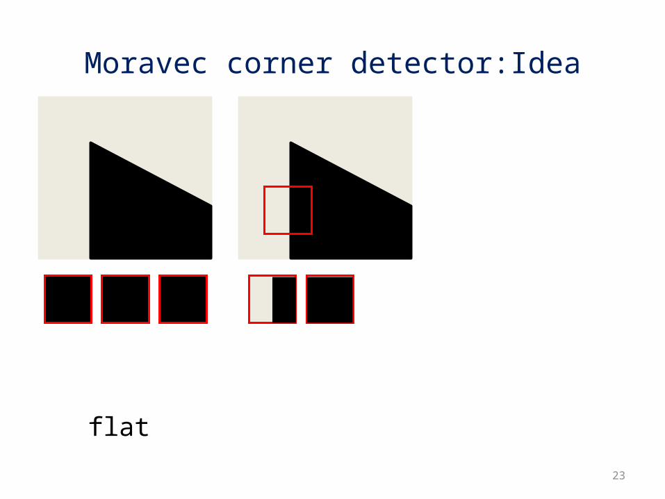
23
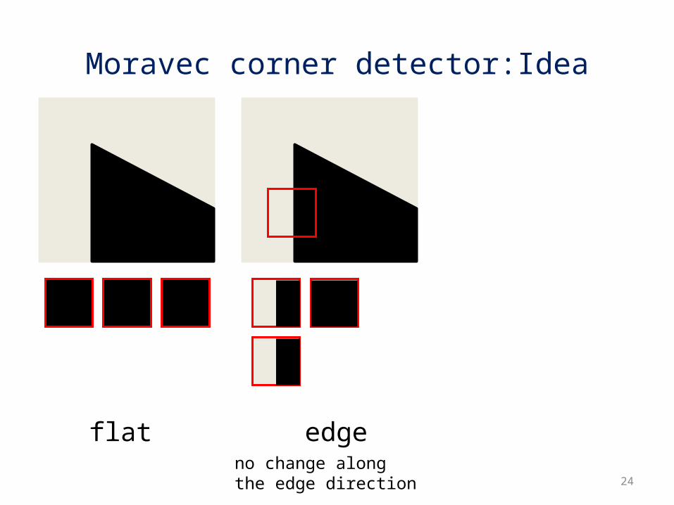
Moravec corner detector:Idea
flat
24
Moravec corner detector:Idea
flat edgeno change along the edge direction
25
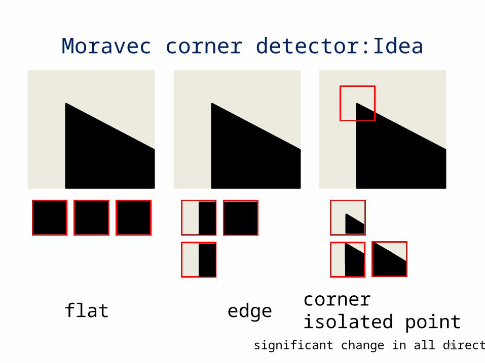
Moravec corner detector:Idea
flat edgecornerisolated point
significant change in all directions
26
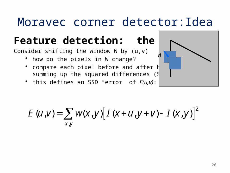
Feature detection: the mathConsider shifting the window W by (u,v)
• how do the pixels in W change?• compare each pixel before and after by
summing up the squared differences (SSD)• this defines an SSD “error” of E(u,v):
Moravec corner detector:Idea
W
2
,
( , ) ( , ) ( , ) ( , )x y
E u v w x y I x u y v I x y
27
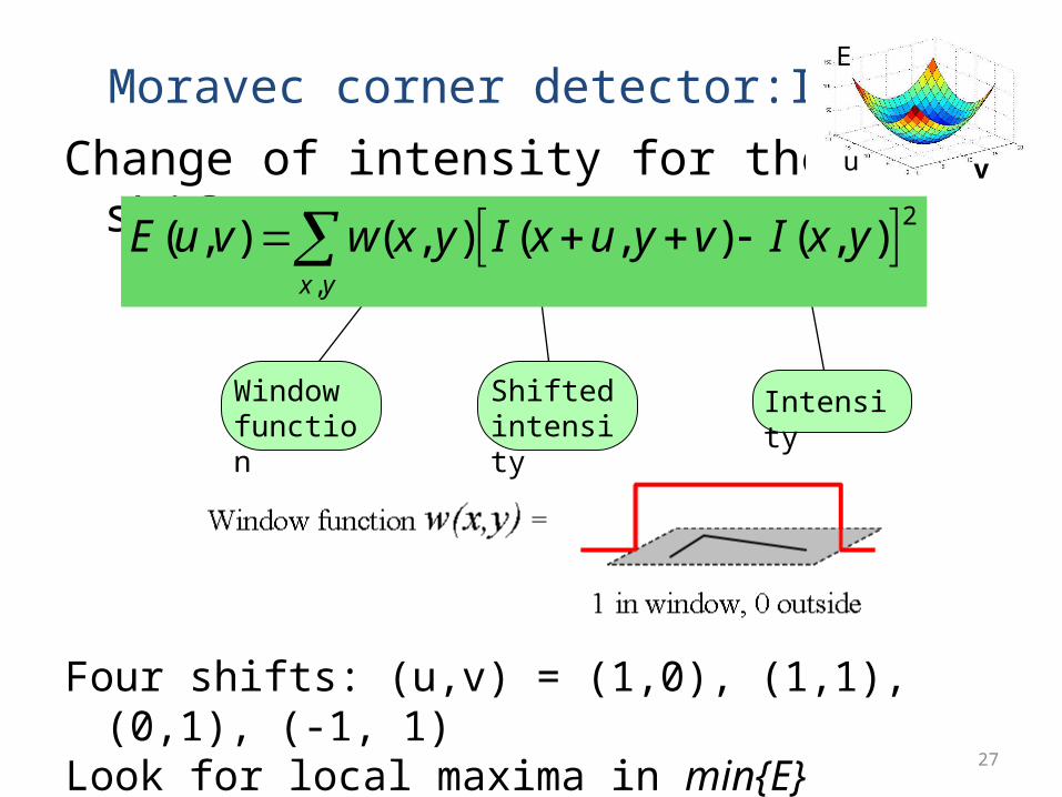
Moravec corner detector:IdeaChange of intensity for the shift [u,v]:
2
,
( , ) ( , ) ( , ) ( , )x y
E u v w x y I x u y v I x y
IntensityShifted intensity
Window function
Four shifts: (u,v) = (1,0), (1,1), (0,1), (-1, 1)Look for local maxima in min{E}
E
u v
28
29
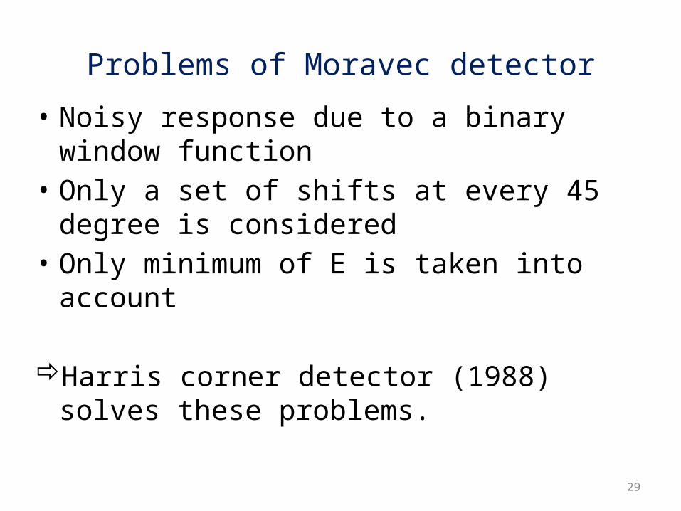
Problems of Moravec detector
• Noisy response due to a binary window function
• Only a set of shifts at every 45 degree is considered
• Only minimum of E is taken into account
Harris corner detector (1988) solves these problems.
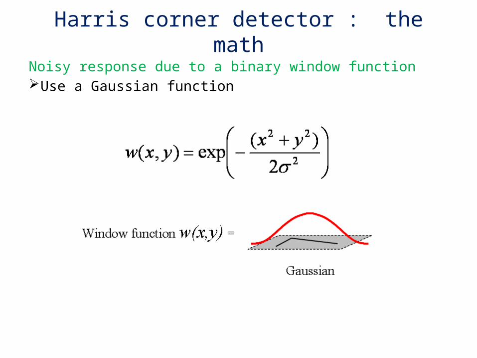
Harris corner detector : the math
Noisy response due to a binary window function Use a Gaussian function
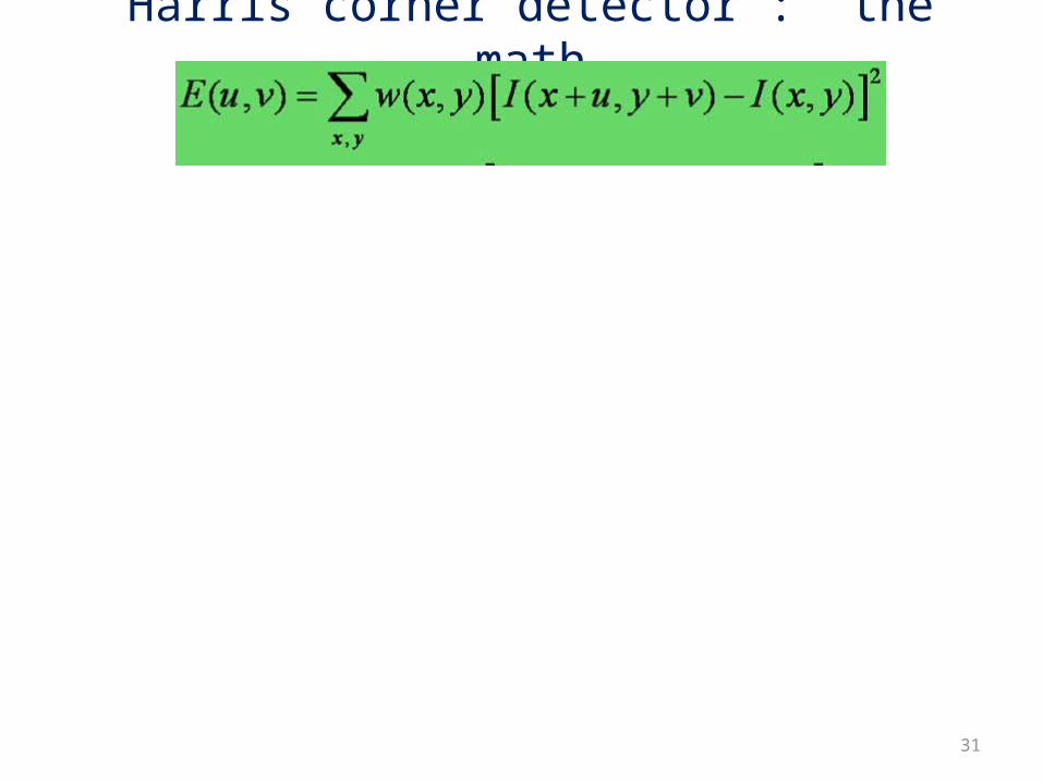
31
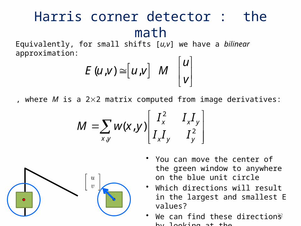
Harris corner detector : the math
32
Harris corner detector : the math
( , ) ,u
E u v u v Mv
Equivalently, for small shifts [u,v] we have a bilinear approximation:
2
2,
( , ) x x y
x y x y y
I I IM w x y
I I I
, where M is a 22 matrix computed from image derivatives:
• You can move the center of the green window to anywhere on the blue unit circle
• Which directions will result in the largest and smallest E values?
• We can find these directions by looking at the eigenvectors of M
33
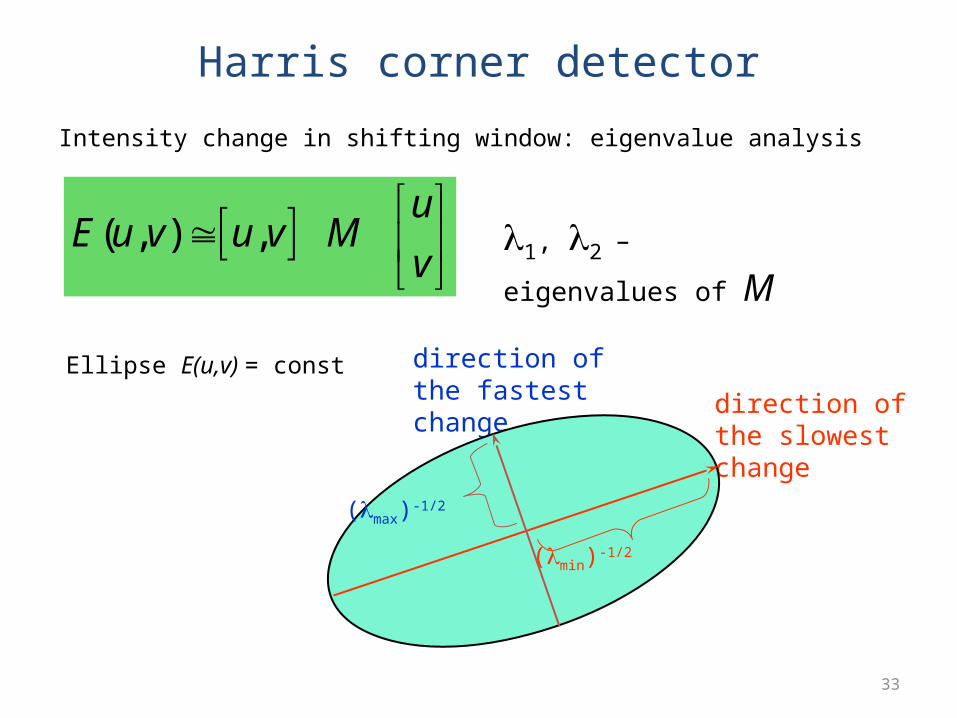
Harris corner detector
( , ) ,u
E u v u v Mv
Intensity change in shifting window: eigenvalue analysis
1, 2 – eigenvalues of M
direction of the slowest change
direction of the fastest change
(max)-1/2
(min)-1/2
Ellipse E(u,v) = const
34
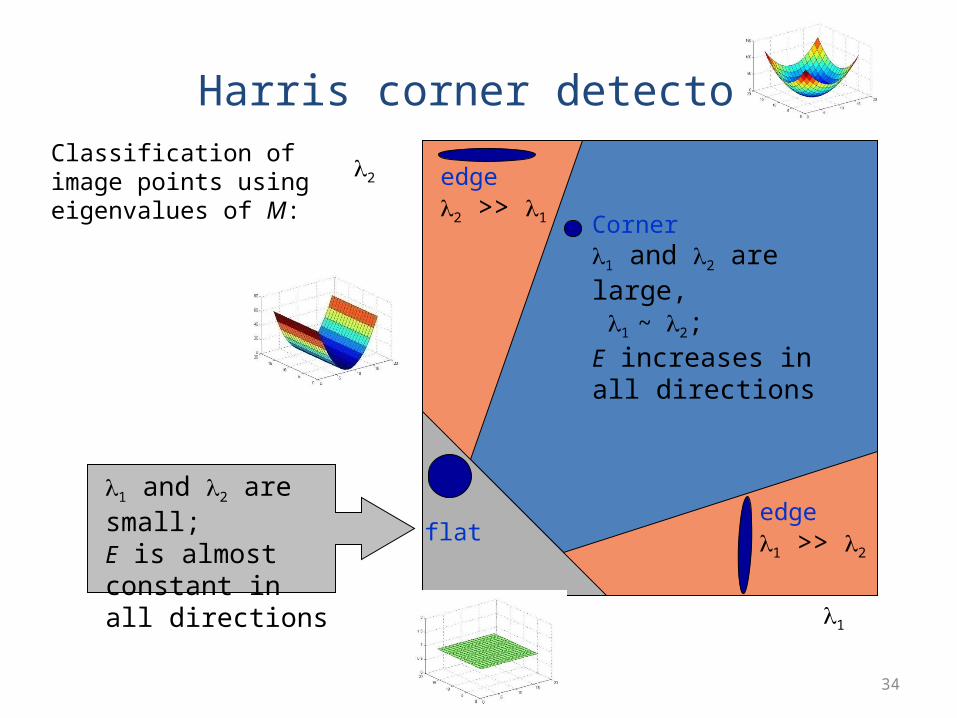
Harris corner detector
1
2
Corner1 and 2 are large, 1 ~ 2;E increases in all directions
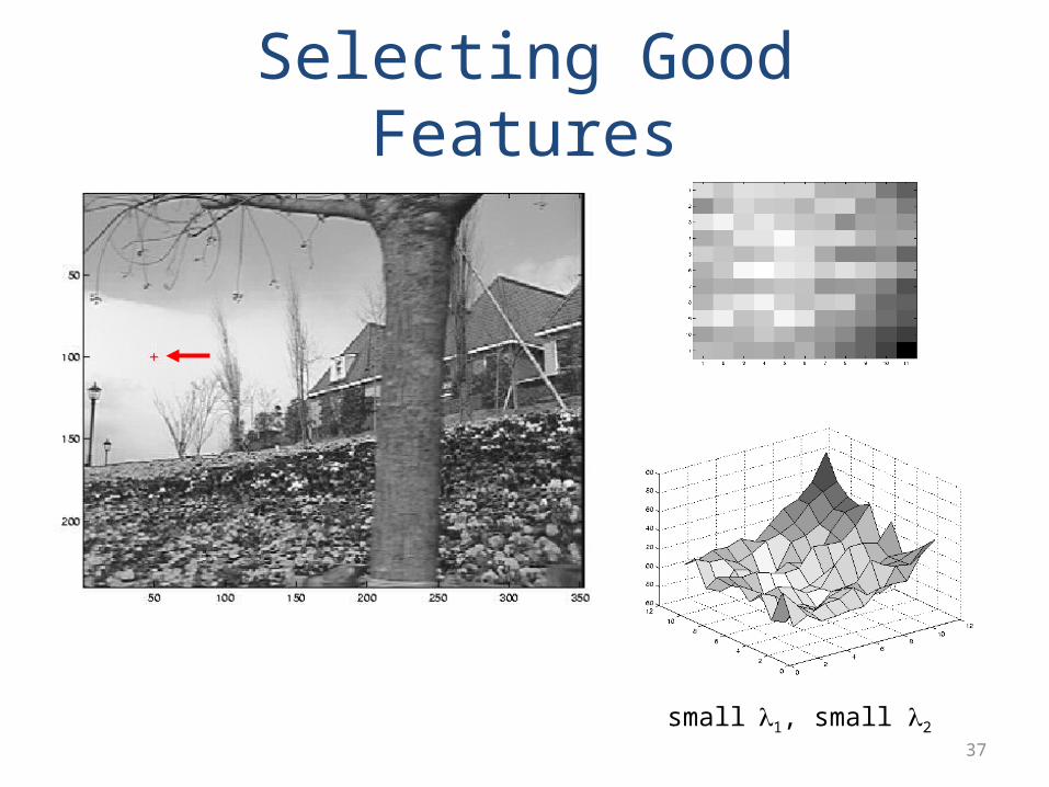
1 and 2 are small;E is almost constant in all directions
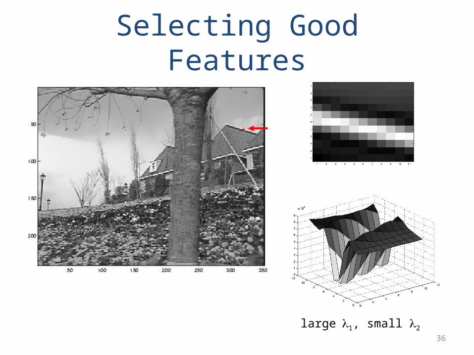
edge 1 >> 2
edge 2 >> 1
flat
Classification of image points using eigenvalues of M:
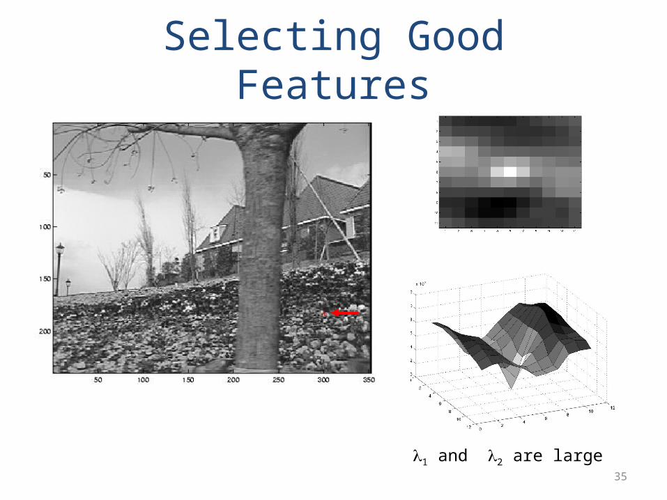
35
Selecting Good Features
l1 and l2 are large
36
Selecting Good Features
large l1, small l2
37
Selecting Good Features
small l1, small l2
Harris corner detector: the mathResponds too strong for edges because only minimum of E is taken into accountA new corner measurement
39
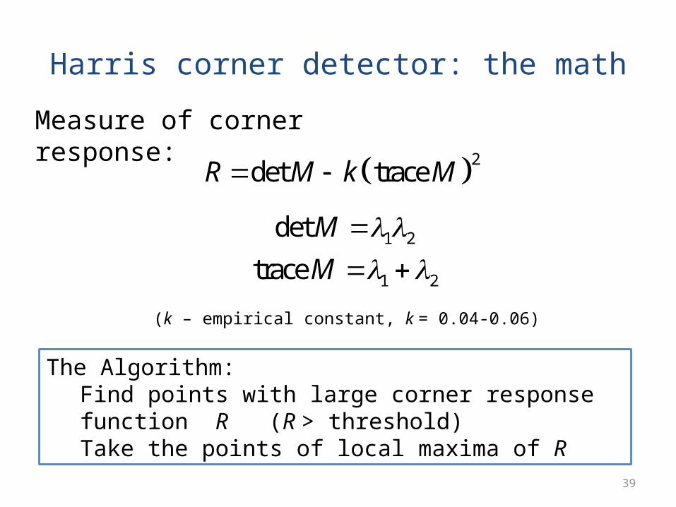
Harris corner detector: the math
Measure of corner response:
2det traceR M k M
1 2
1 2
det
trace
M
M
(k – empirical constant, k = 0.04-0.06)
The Algorithm:Find points with large corner response function R (R > threshold)Take the points of local maxima of R
40
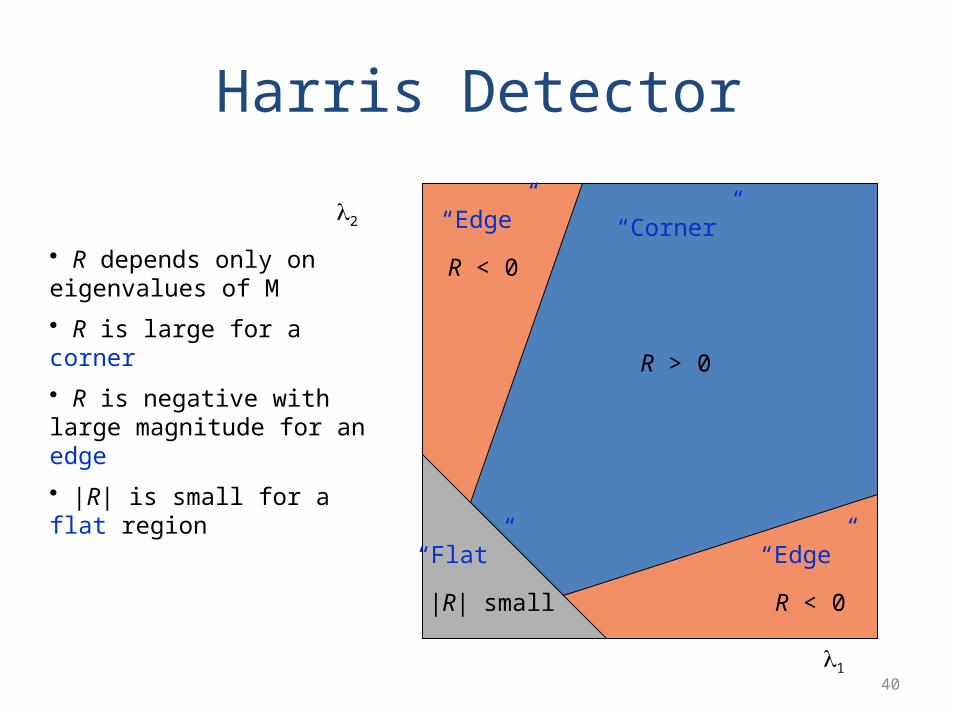
Harris Detector
1
2 “Corner”
“Edge”
“Edge”
“Flat”
• R depends only on eigenvalues of M
• R is large for a corner
• R is negative with large magnitude for an edge
• |R| is small for a flat region
R > 0
R < 0
R < 0|R| small
41
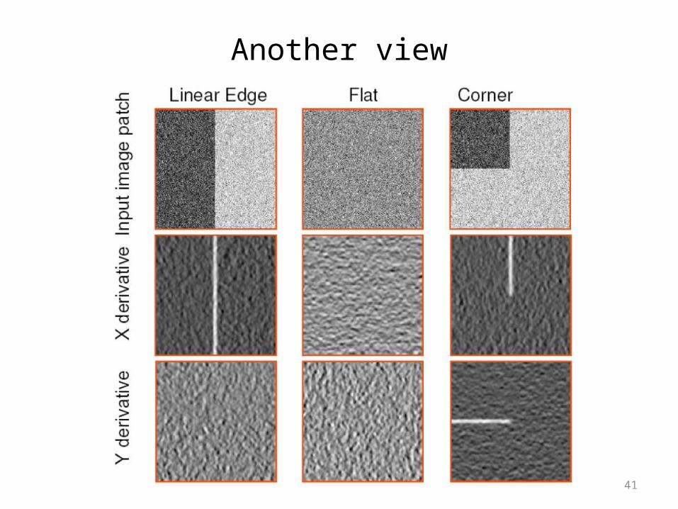
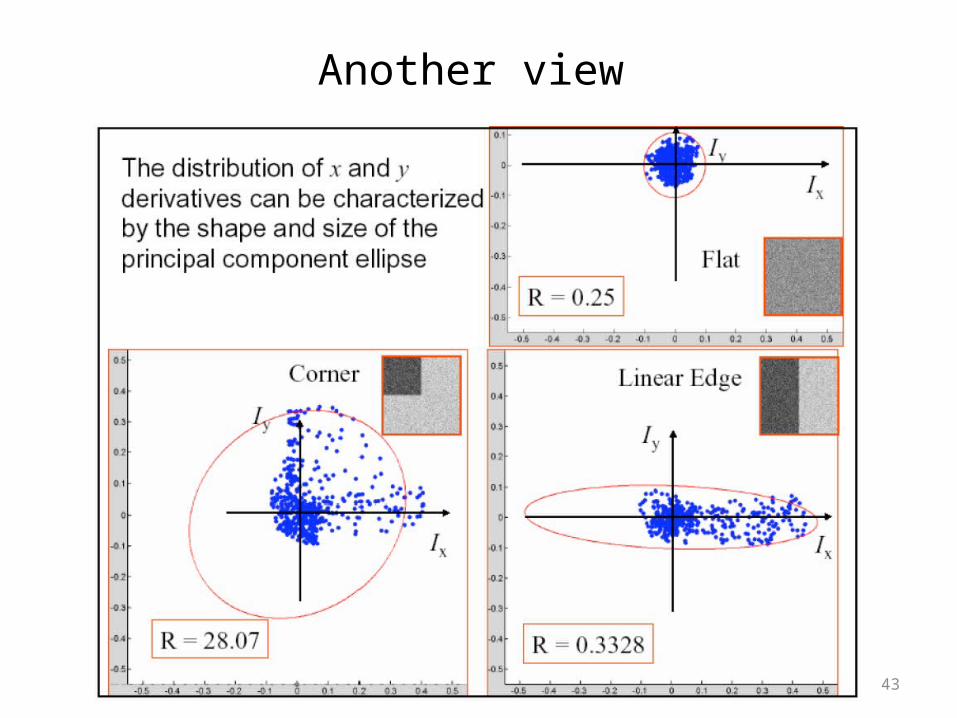
Another view
42
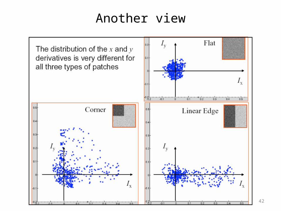
Another view
43
Another view
44
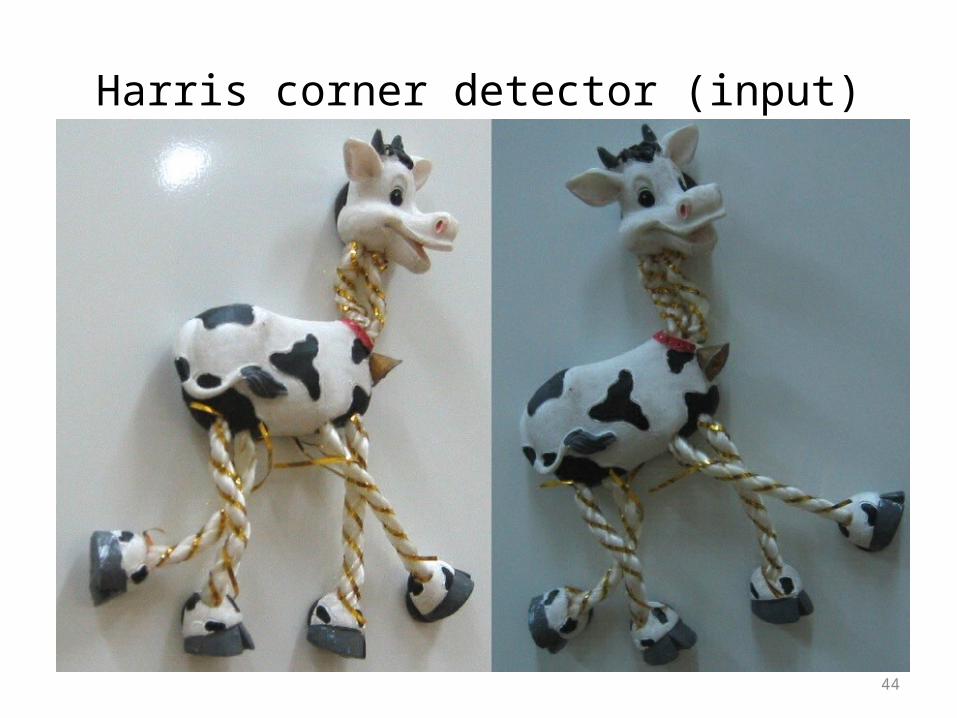
Harris corner detector (input)
45
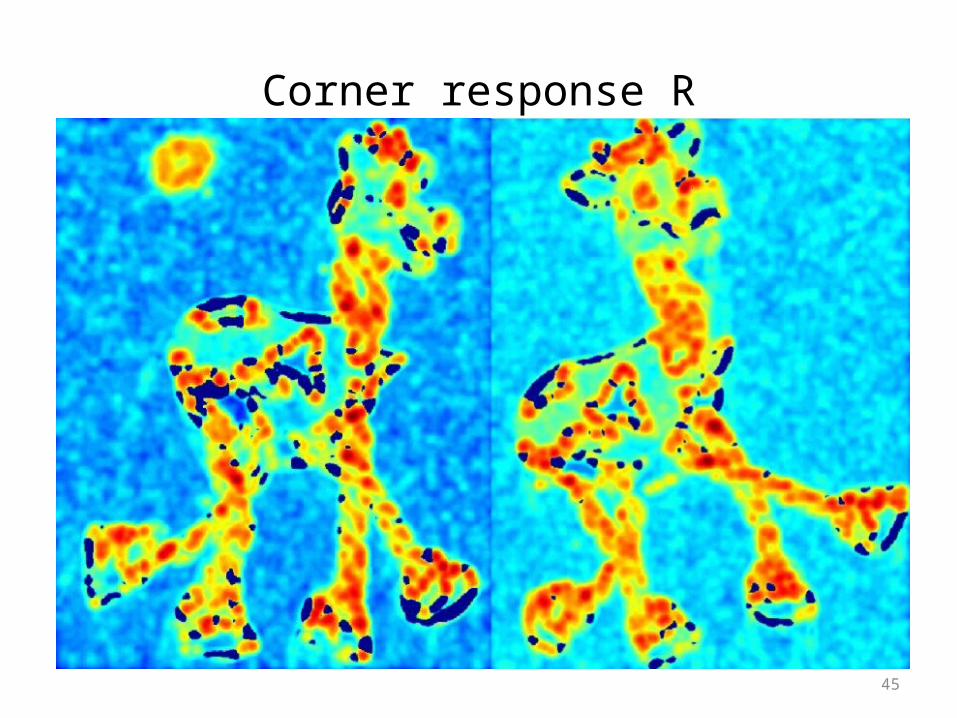
Corner response R
46
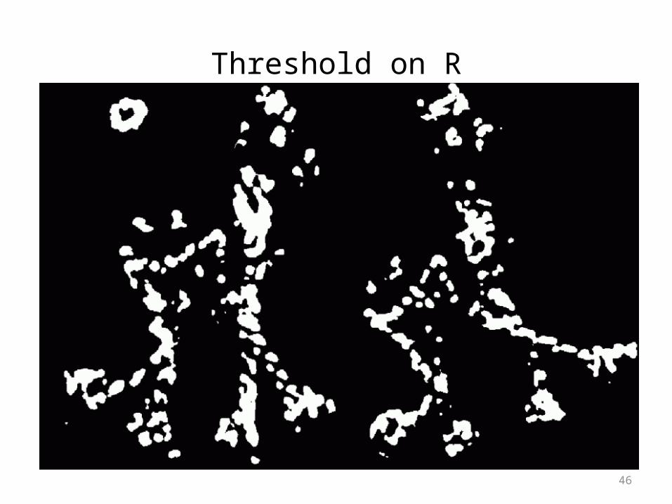
Threshold on R
47
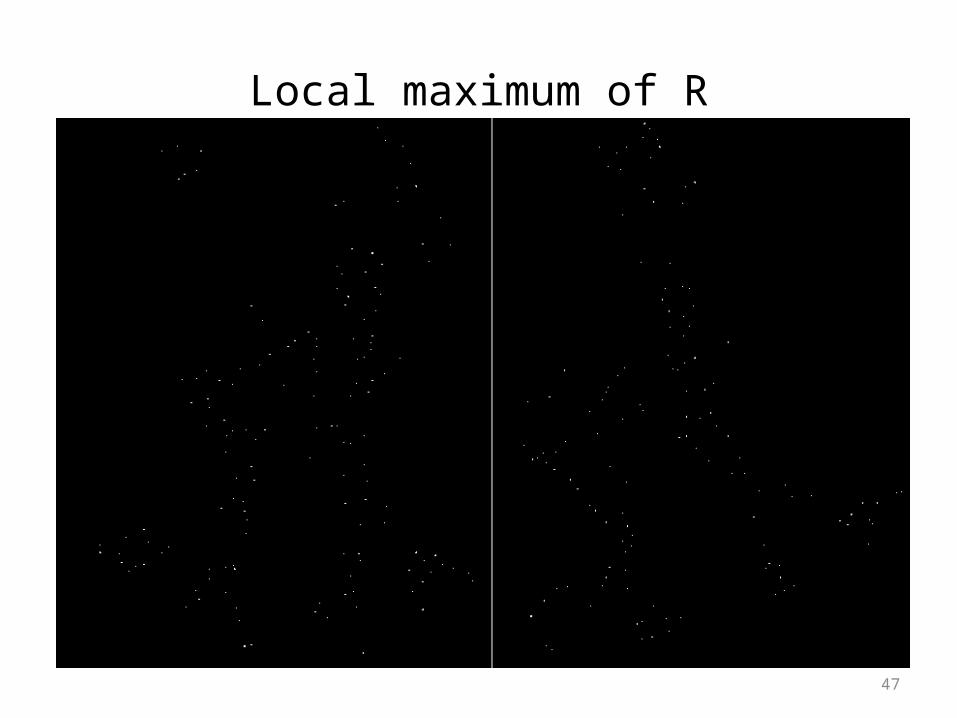
Local maximum of R
48
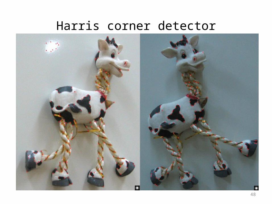
Harris corner detector
49
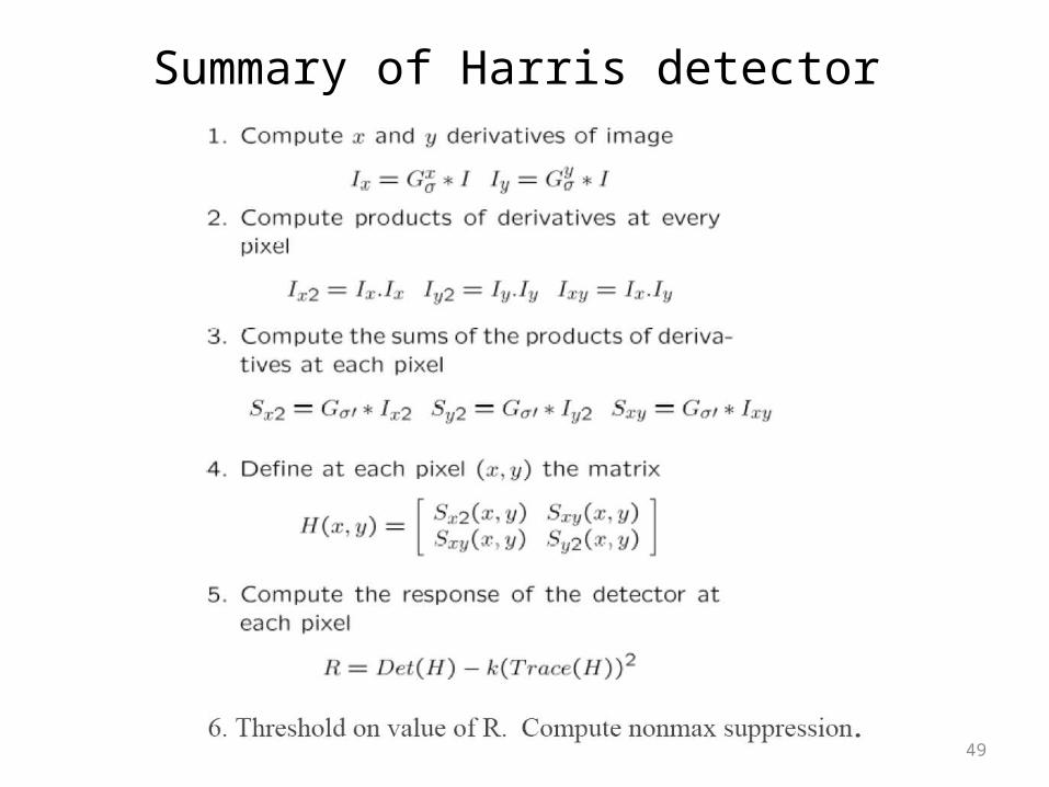
Summary of Harris detector
50
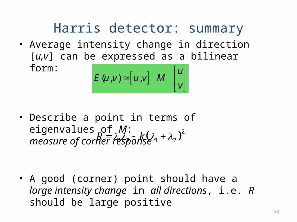
Harris detector: summary• Average intensity change in direction [u,v] can be
expressed as a bilinear form:
• Describe a point in terms of eigenvalues of M:measure of corner response
• A good (corner) point should have a large intensity change in all directions, i.e. R should be large positive
( , ) ,u
E u v u v Mv
2
1 2 1 2R k
51
Harris Detector: Some Properties
• Invariance to image intensity change?
52
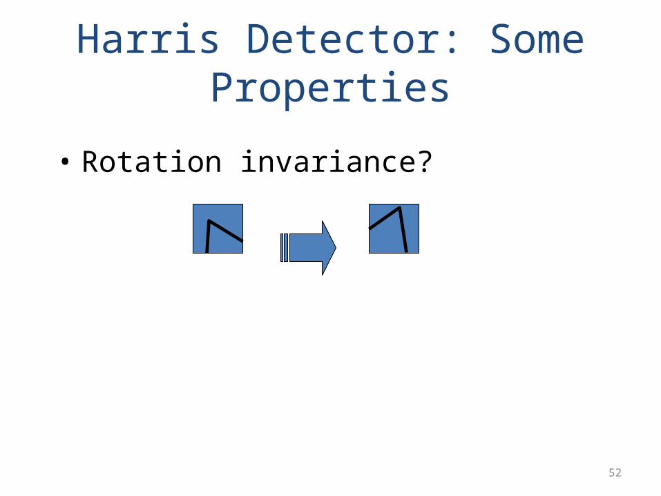
Harris Detector: Some Properties
• Rotation invariance?
53
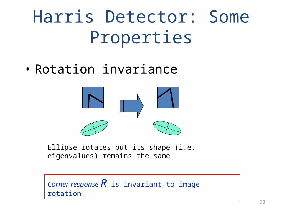
Harris Detector: Some Properties
• Rotation invariance
Ellipse rotates but its shape (i.e. eigenvalues) remains the same
Corner response R is invariant to image rotation
54
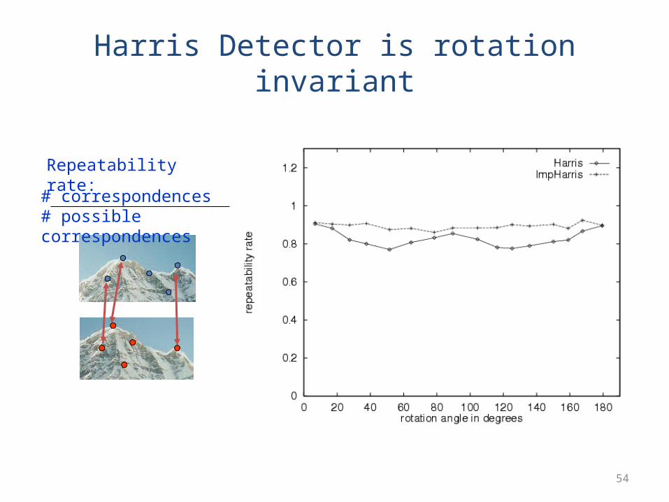
Harris Detector is rotation invariant
Repeatability rate:
# correspondences# possible correspondences
55
Harris Detector: Some Properties
• Invariant to image scale?
56
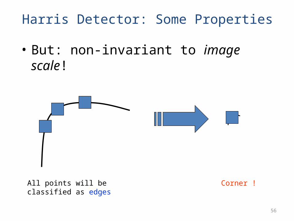
Harris Detector: Some Properties
• But: non-invariant to image scale!
All points will be classified as edges
Corner !
57
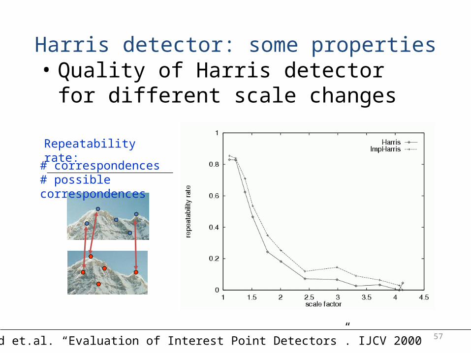
Harris detector: some properties• Quality of Harris detector for different scale
changes
Repeatability rate:
# correspondences# possible correspondences
C.Schmid et.al. “Evaluation of Interest Point Detectors”. IJCV 2000
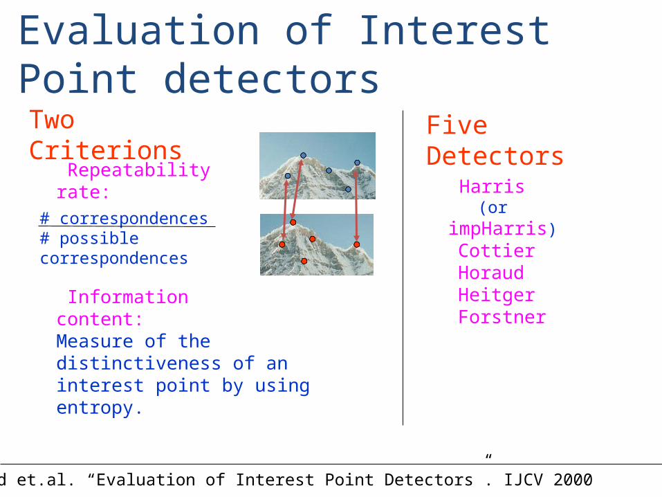
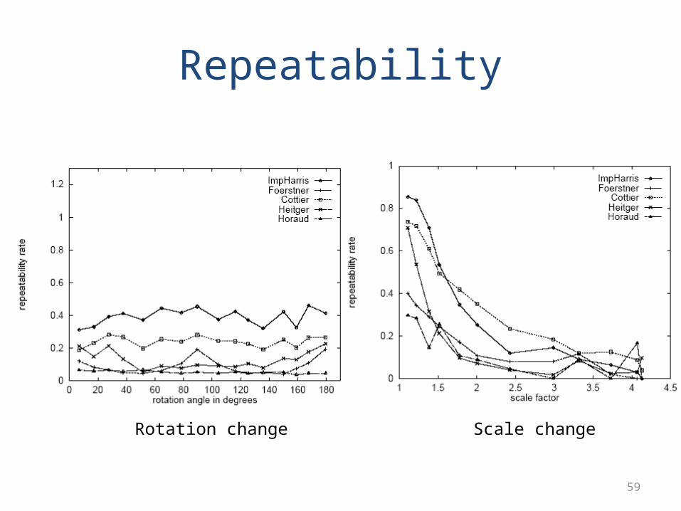
Evaluation of Interest Point detectorsTwo Criterions
Repeatability rate:
# correspondences# possible correspondences
Information content:
Measure of the distinctiveness of an interest point by using entropy.
C.Schmid et.al. “Evaluation of Interest Point Detectors”. IJCV 2000
Five Detectors
Harris (or impHarris) Cottier Horaud Heitger Forstner
59
Repeatability
Rotation change Scale change
60
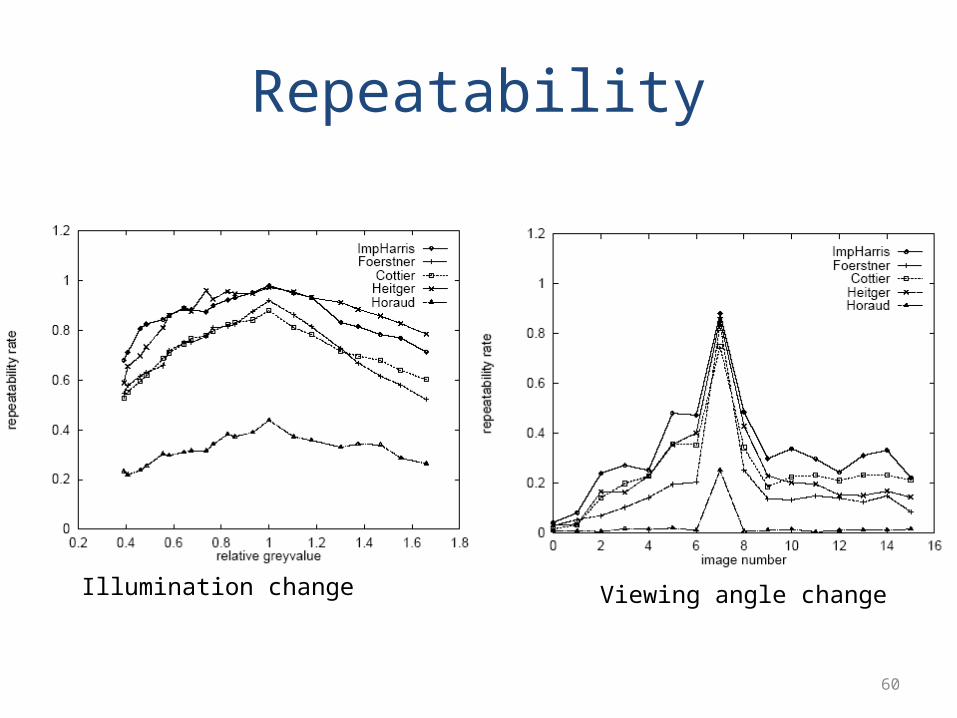
Repeatability
Illumination change Viewing angle change
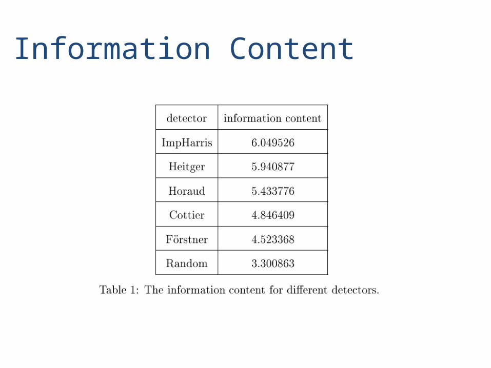
Information Content
62
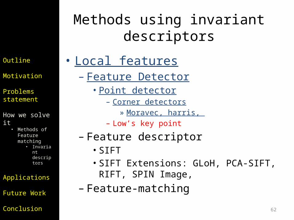
Methods using invariant descriptors
• Local features– Feature Detector
• Point detector– Corner detectors
» Moravec, harris, – Low’s key point
– Feature descriptor• SIFT• SIFT Extensions: GLoH, PCA-SIFT, RIFT, SPIN
Image,
– Feature-matching
Outline
Motivation
Problems statement
How we solve it
• Methods of Feature matching
• Invariant descriptors
Applications
Future Work
Conclusion
63
We want to:
detect the same interest points regardless of image changes
64
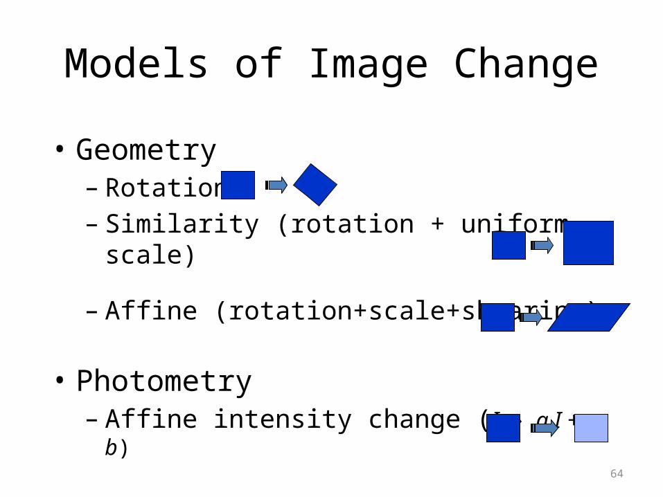
Models of Image Change
• Geometry– Rotation– Similarity (rotation + uniform scale)
– Affine (rotation+scale+shearing)
• Photometry– Affine intensity change (I a I + b)
65
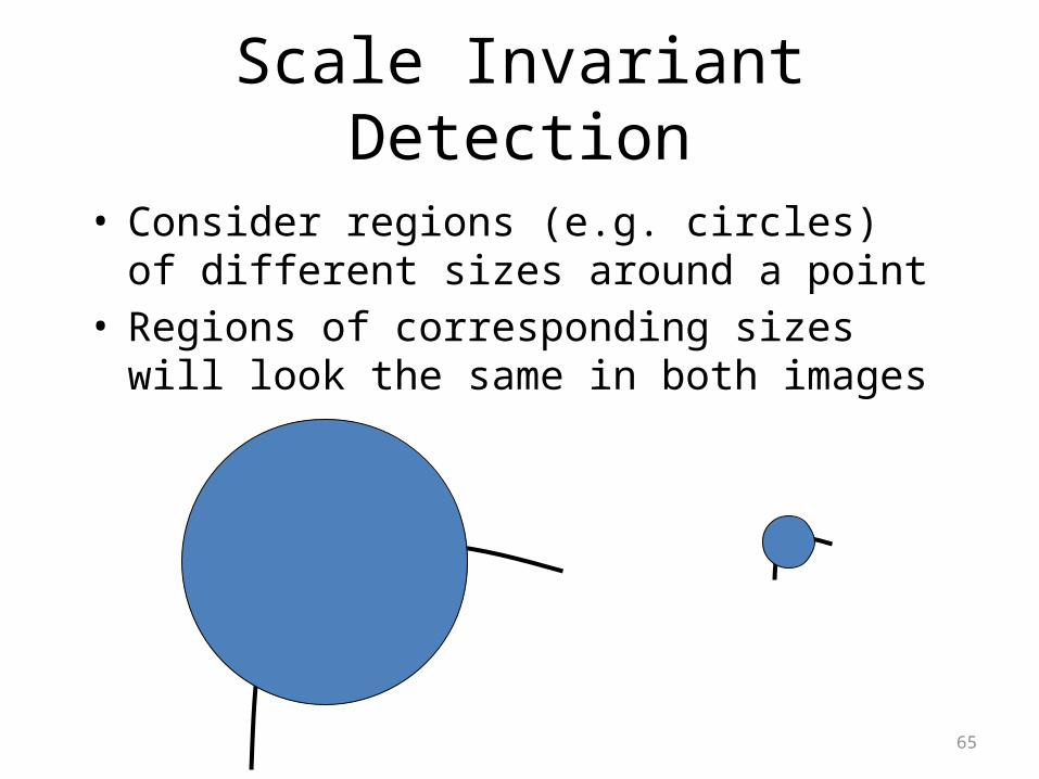
Scale Invariant Detection
• Consider regions (e.g. circles) of different sizes around a point
• Regions of corresponding sizes will look the same in both images
66
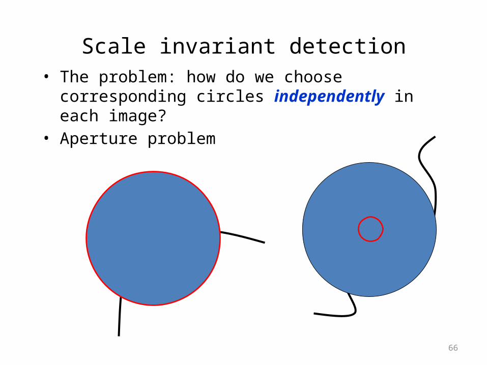
Scale invariant detection• The problem: how do we choose corresponding circles
independently in each image?• Aperture problem
67
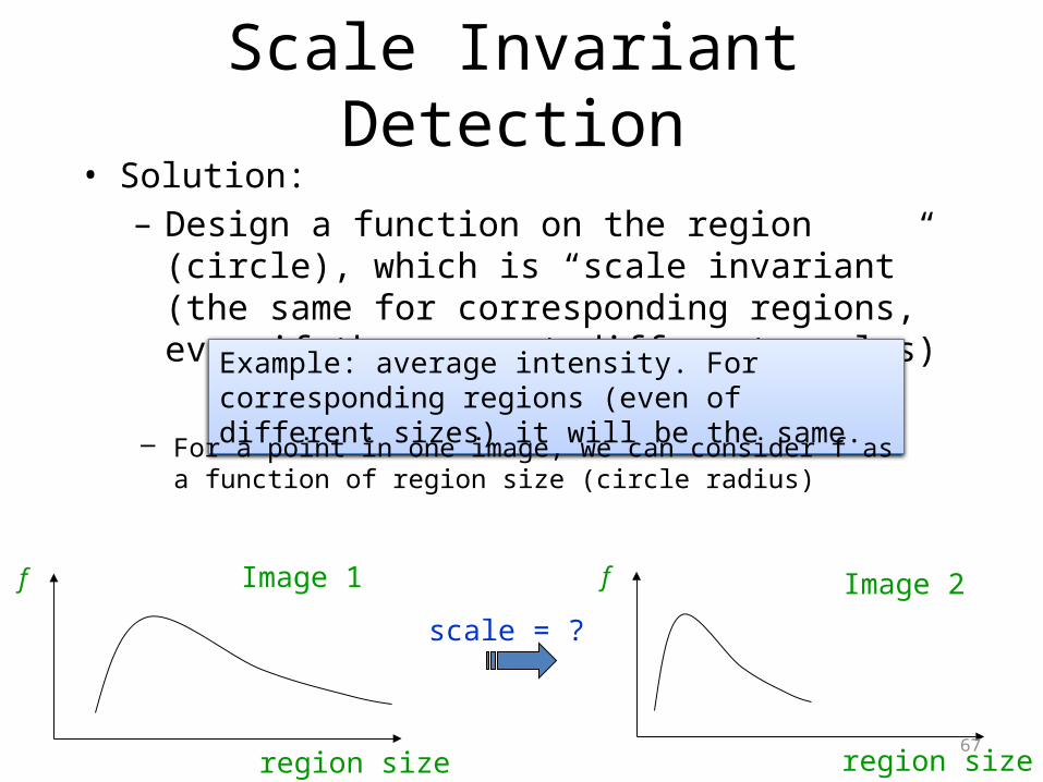
Scale Invariant Detection• Solution:
– Design a function on the region (circle), which is “scale invariant” (the same for corresponding regions, even if they are at different scales)
Example: average intensity. For corresponding regions (even of different sizes) it will be the same.
– For a point in one image, we can consider f as a function of region size (circle radius)
f
region size
Image 1 f
region size
Image 2
scale = ?
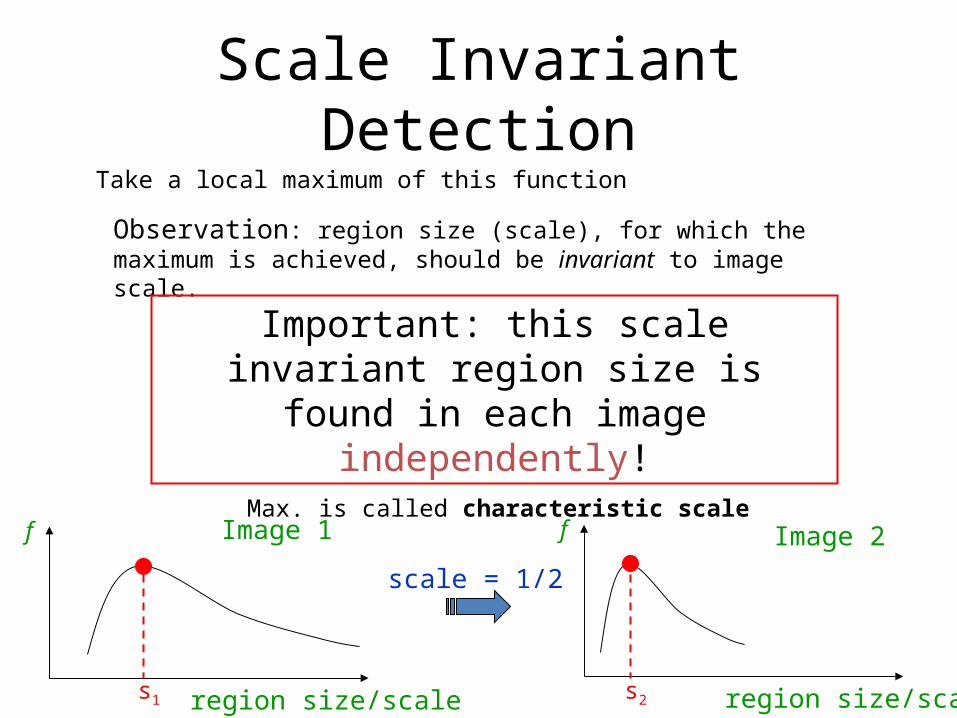
Scale Invariant Detection
scale = 1/2
f
region size/scale
Image 1 f
region size/scale
Image 2
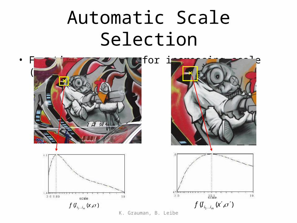
Take a local maximum of this function
Observation: region size (scale), for which the maximum is achieved, should be invariant to image scale.
s1 s2
Important: this scale invariant region size is found in each image independently!
Max. is called characteristic scale
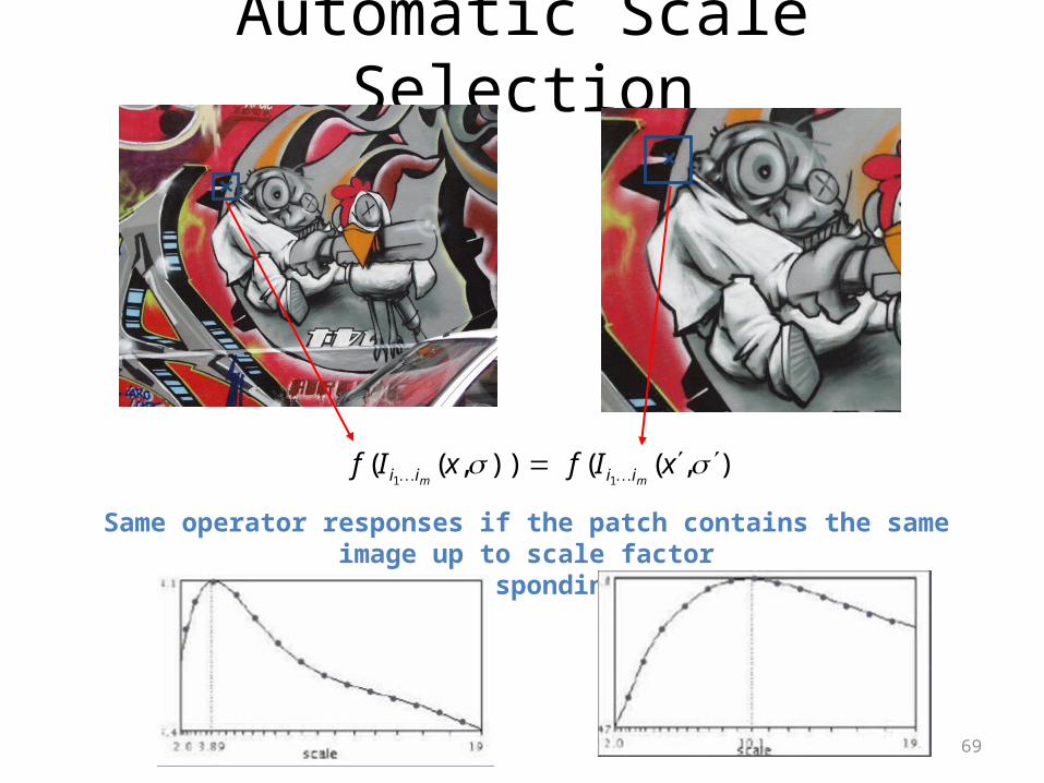
Automatic Scale Selection
69
)),(( )),((11
xIfxIfmm iiii
Same operator responses if the patch contains the same image up to scale factorHow to find corresponding patch sizes?
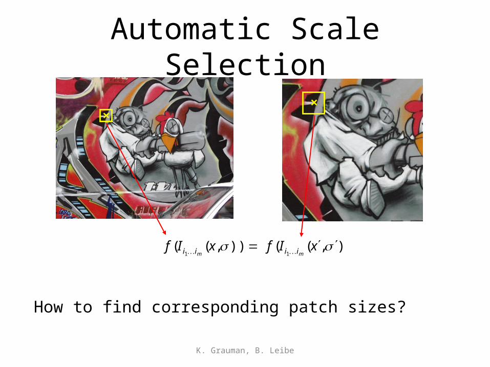
Automatic Scale Selection
K. Grauman, B. Leibe
)),(( )),((11
xIfxIfmm iiii
How to find corresponding patch sizes?

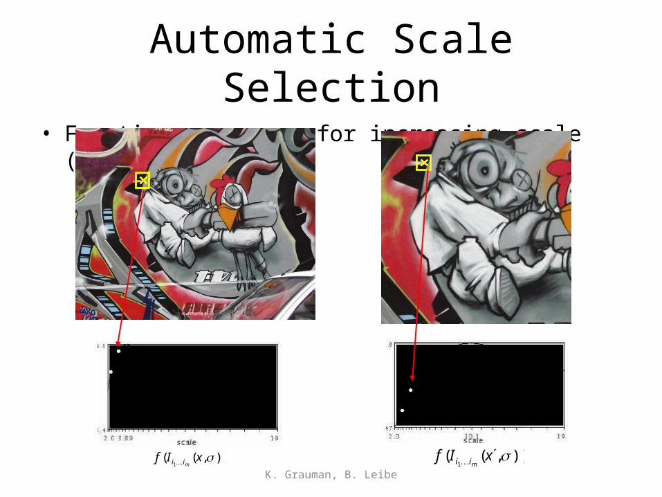
Automatic Scale Selection
• Function responses for increasing scale (scale signature)
K. Grauman, B. Leibe)),((
1xIf
mii )),((1
xIfmii
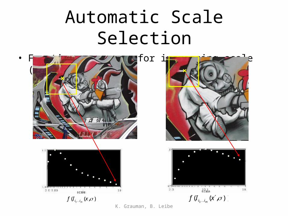
Automatic Scale Selection
• Function responses for increasing scale (scale signature)
K. Grauman, B. Leibe)),((
1xIf
mii )),((1
xIfmii

Automatic Scale Selection
• Function responses for increasing scale (scale signature)
K. Grauman, B. Leibe)),((
1xIf
mii )),((1
xIfmii

Automatic Scale Selection
• Function responses for increasing scale (scale signature)
K. Grauman, B. Leibe)),((
1xIf
mii )),((1
xIfmii
Automatic Scale Selection
• Function responses for increasing scale (scale signature)
K. Grauman, B. Leibe)),((
1xIf
mii )),((1
xIfmii
Automatic Scale Selection
• Function responses for increasing scale (scale signature)
K. Grauman, B. Leibe)),((
1xIf
mii )),((1
xIfmii
77
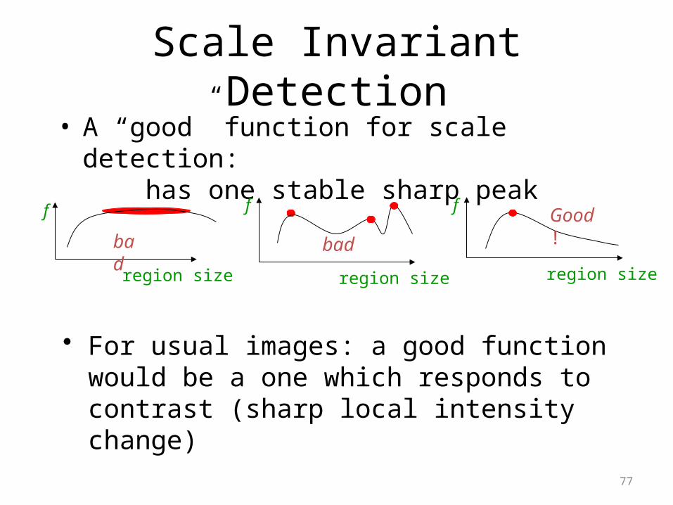
Scale Invariant Detection• A “good” function for scale detection:
has one stable sharp peak
f
region size
bad
f
region size
bad
f
region size
Good !
• For usual images: a good function would be a one which responds to contrast (sharp local intensity change)
78
Scale Invariant Detection• Laplacian-of-Gaussian (LoG)• Difference of Gaussian (DOG)
79
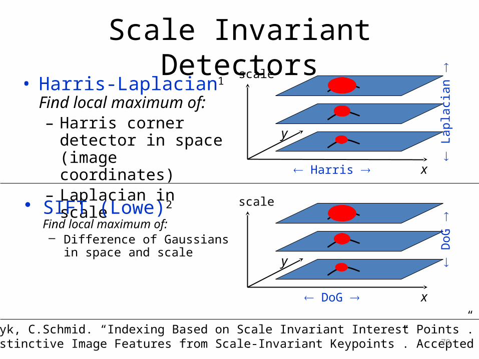
Scale Invariant Detectors• Harris-Laplacian1
Find local maximum of:– Harris corner detector in
space (image coordinates)– Laplacian in scale
1 K.Mikolajczyk, C.Schmid. “Indexing Based on Scale Invariant Interest Points”. ICCV 20012 D.Lowe. “Distinctive Image Features from Scale-Invariant Keypoints”. Accepted to IJCV 2004
scale
x
y
Harris
Lap
laci
an
• SIFT (Lowe)2
Find local maximum of:– Difference of Gaussians in space
and scale
scale
x
y
DoG
DoG
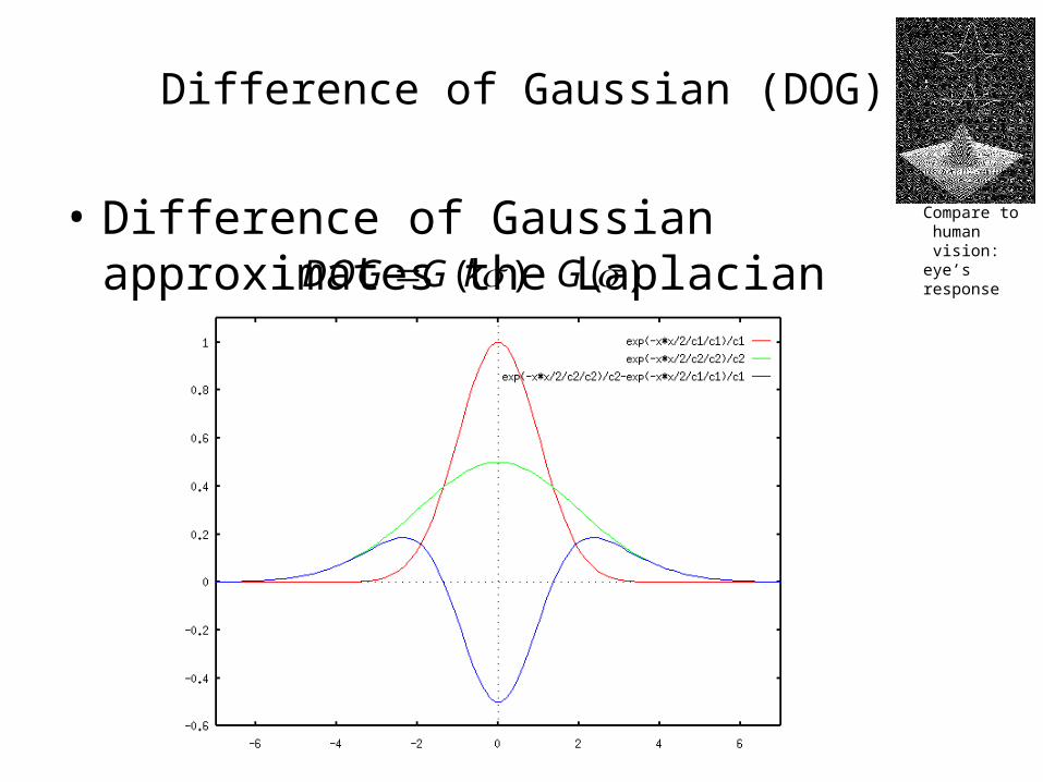
Difference of Gaussian (DOG)
• Difference of Gaussian approximates the Laplacian )()( GkGDOG
Compare to human vision: eye’s response
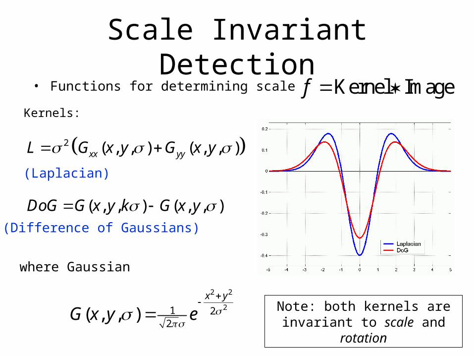
Scale Invariant Detection• Functions for determining scale
2 2
21 22
( , , )x y
G x y e
2 ( , , ) ( , , )xx yyL G x y G x y
( , , ) ( , , )DoG G x y k G x y
Kernel Imagef Kernels:
where Gaussian
Note: both kernels are invariant to scale and rotation
(Laplacian)
(Difference of Gaussians)
82
Scale Invariant Detection• Laplacian-of-Gaussian (LoG)• Difference of Gaussian (DOG)
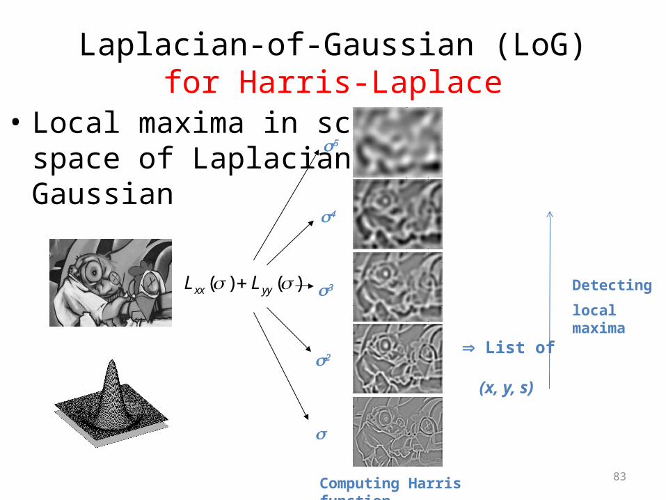
Laplacian-of-Gaussian (LoG)for Harris-Laplace
• Local maxima in scale space of Laplacian-of-Gaussian
83
)()( yyxx LL
s
s2
s3
s4
s5
List of (x, y, s)
Computing Harris function
Detecting
local maxima
84
Harris-Laplace
• Two Parts:– Multiscale-Harris detector– Characteristic scale identification
85
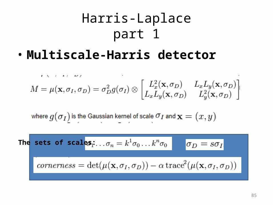
Harris-Laplacepart 1
• Multiscale-Harris detector
The sets of scales:
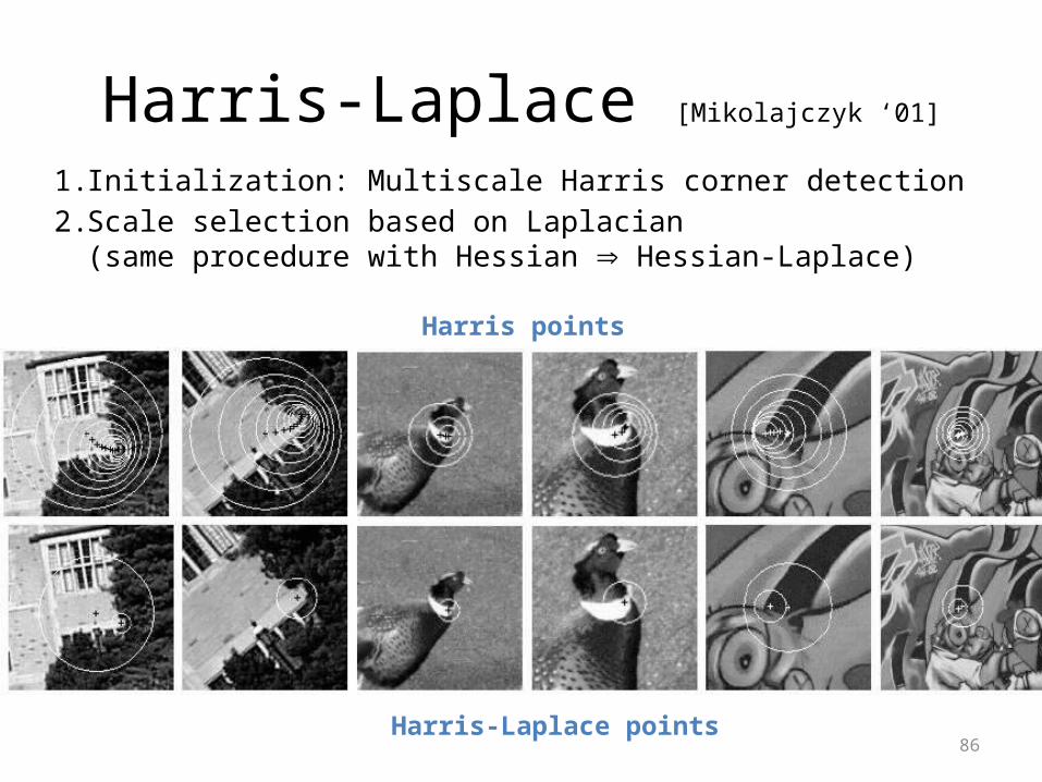
Harris-Laplace [Mikolajczyk ‘01]
1. Initialization: Multiscale Harris corner detection2. Scale selection based on Laplacian
(same procedure with Hessian Hessian-Laplace)
86
Harris points
Harris-Laplace points
87
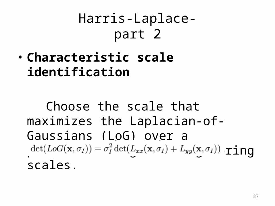
Harris-Laplace-part 2
• Characteristic scale identification
Choose the scale that maximizes the Laplacian-of-Gaussians (LoG) over a predefined range of neighboring scales.
88
Scale Invariant Detection• Laplacian-of-Gaussian (LoG)• Difference of Gaussian (DOG)
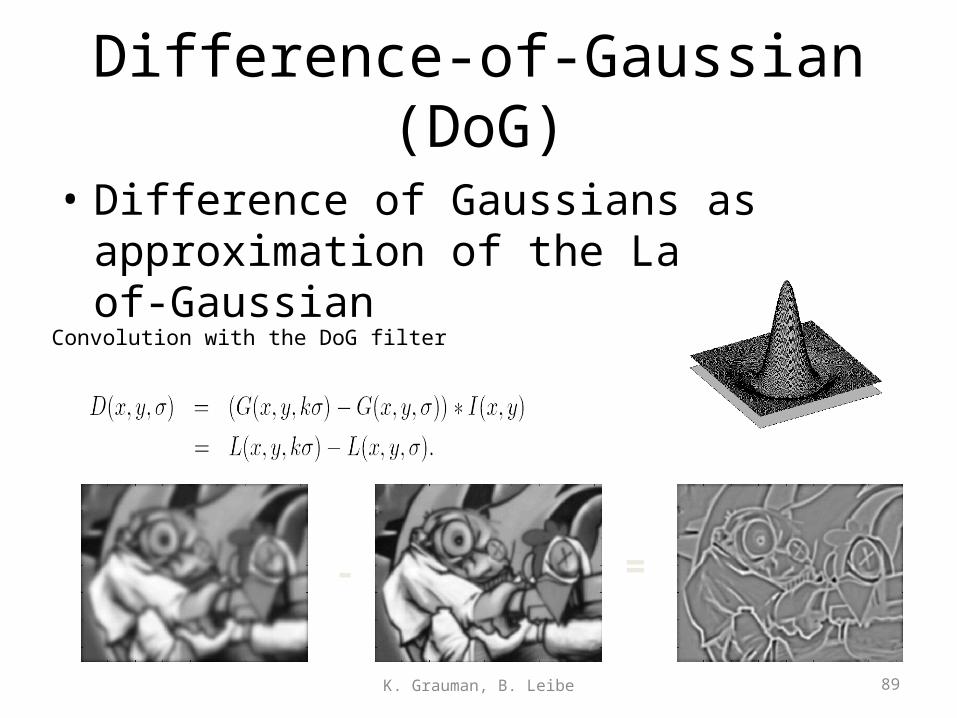
Difference-of-Gaussian (DoG)
• Difference of Gaussians as approximation of the Laplacian-of-Gaussian
89K. Grauman, B. Leibe
- =
Convolution with the DoG filter
90
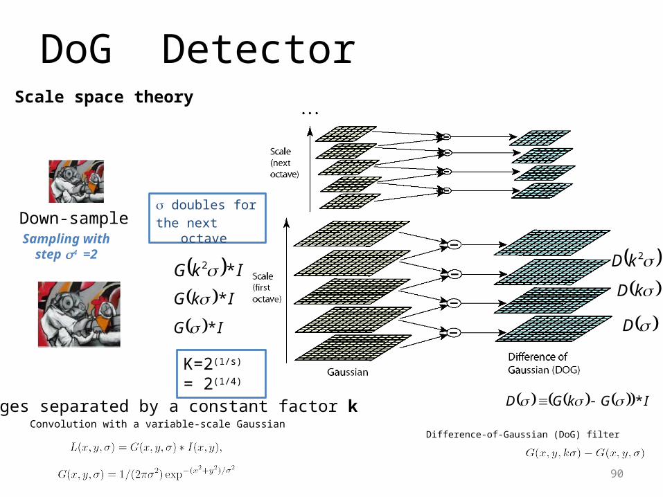
DoG DetectorScale space theory
Down-sample doubles for the next octave
K=2(1/s) = 2(1/4)
IkG *
IG *
IkG *2
IGkGD * Images separated by a constant factor k
D
kD
2kD
Convolution with a variable-scale GaussianDifference-of-Gaussian (DoG) filter
Sampling withstep s4 =2
91
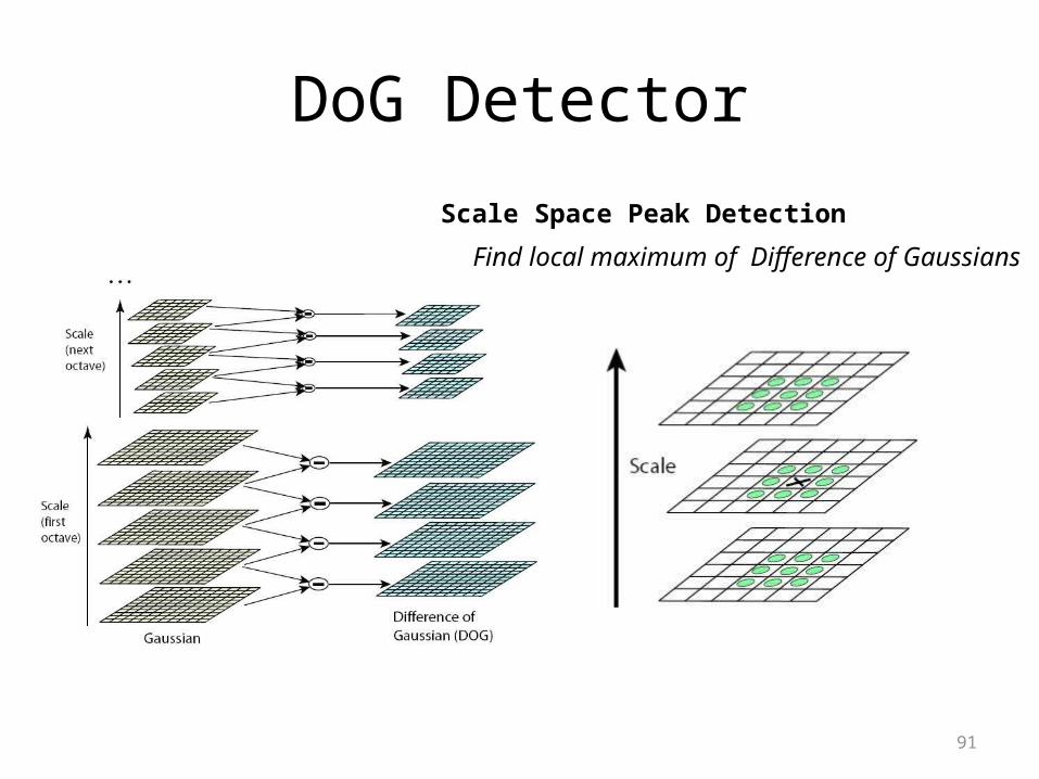
DoG Detector
Scale Space Peak Detection
Find local maximum of Difference of Gaussians
92
1. Detection of scale-space extrema
• For scale invariance, search for stable features across all possible scales using a continuous function of scale, scale space.
• SIFT uses DoG filter for scale space because it is efficient and as stable as scale-normalized Laplacian of Gaussian.
93
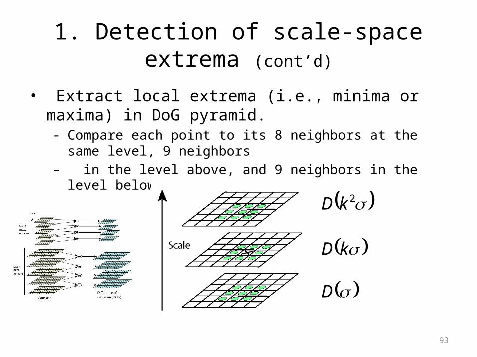
1. Detection of scale-space extrema (cont’d)
• Extract local extrema (i.e., minima or maxima) in DoG pyramid.- Compare each point to its 8 neighbors at the same level, 9 neighbors– in the level above, and 9 neighbors in the level below (i.e., 26 total).
D
kD
2kD
94
Choosing SIFT parameters• Experimentally using a matching task:
- 32 real images (outdoor, faces, aerial etc.)
- Images subjected to a wide range of transformations (i.e., rotation, scaling, shear, change in brightness, noise).
- Keypoints are detected in each image.
- Parameters are chosen based on keypoint repeatability, localization, and matching accuracy.
95
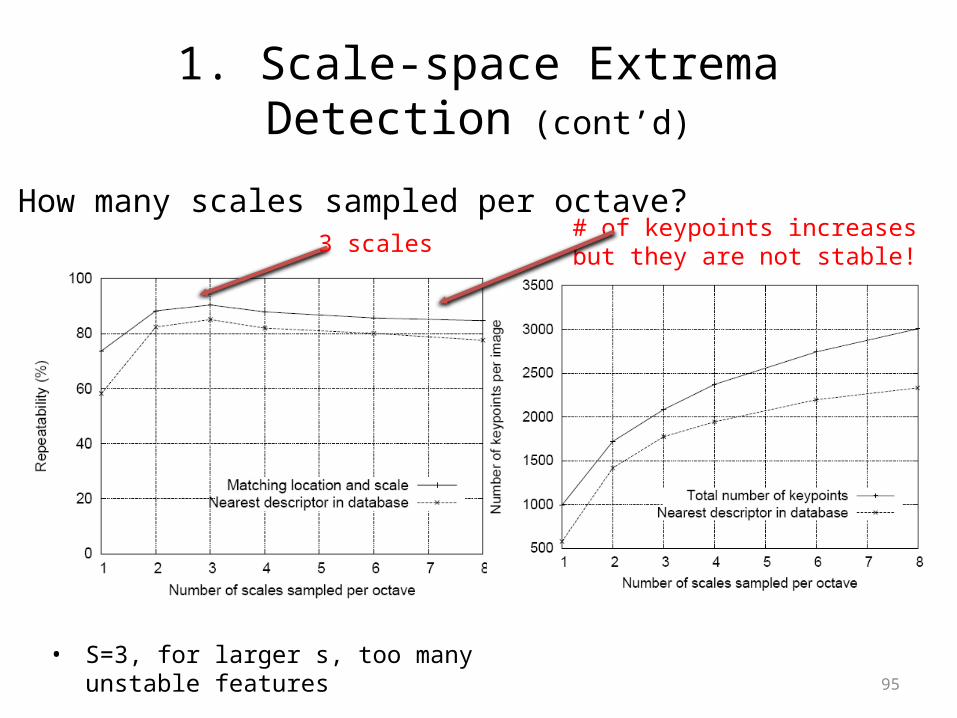
1. Scale-space Extrema Detection (cont’d)
• How many scales sampled per octave?3 scales
• S=3, for larger s, too many unstable features
# of keypoints increases but they are not stable!
96
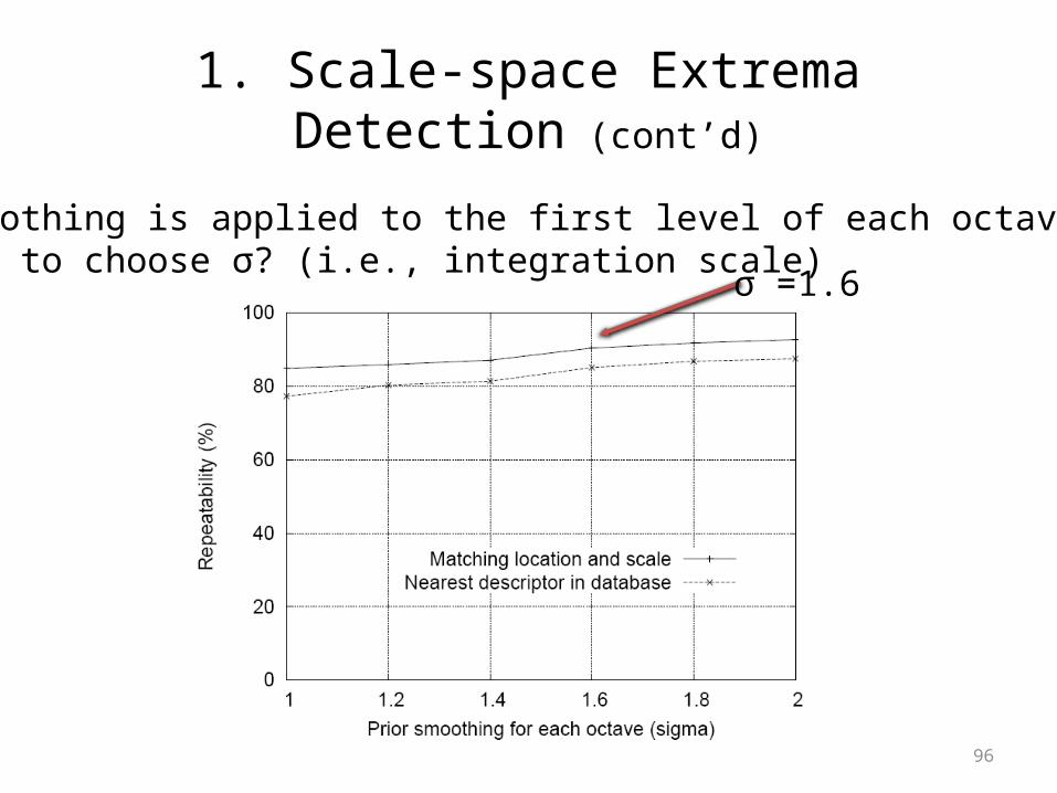
1. Scale-space Extrema Detection (cont’d)
• Smoothing is applied to the first level of each octave.• How to choose σ? (i.e., integration scale)
σ =1.6
97
2. Accurate keypoint localization
• There are still a lot of points, some of them are not good enough.
– The locations of keypoints may be not accurate.– Eliminating edge points.
• Thus– Reject points with low contrast and poorly
localized along an edge– Fit a 3D quadratic function for sub-pixel maxima
98
2. Accurate keypoint localization
• There are still a lot of points, some of them are not good enough.
– The locations of keypoints may be not accurate.– Eliminating edge points.
• Thus– Reject points with low contrast and poorly
localized along an edge– Fit a 3D quadratic function for sub-pixel maxima
99
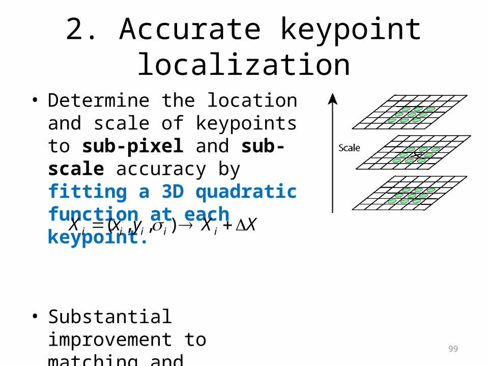
2. Accurate keypoint localization
• Determine the location and scale of keypoints to sub-pixel and sub-scale accuracy by fitting a 3D quadratic function at each keypoint.
• Substantial improvement to matching and stability!
( , , )i i i i iX x y X X
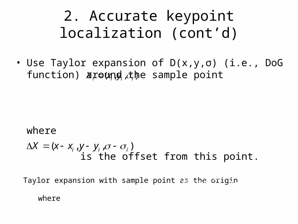
2. Accurate keypoint localization (cont’d)
• Use Taylor expansion of D(x,y,σ) (i.e., DoG function) around the sample point
where is the offset from this point.
2
2
( ) ( )1( ) ( )
2
TTi i
i
D X D XD X D X
( , , )i i iX x x y y
( , , )i i i iX x y
Taylor expansion with sample point as the origin
where
2
2
2
1)(
DDDD T
T
Tyx ),,(

101
2. Accurate keypoint localization (cont’d)
• Change sample point if offset is larger than 0.5
• Throw out low contrast (<0.03)
102
2. Accurate keypoint localization
• There are still a lot of points, some of them are not good enough.
– The locations of keypoints may be not accurate.– Eliminating edge points.
• Thus– Reject points with low contrast and poorly
localized along an edge– Fit a 3D quadratic function for sub-pixel maxima
103
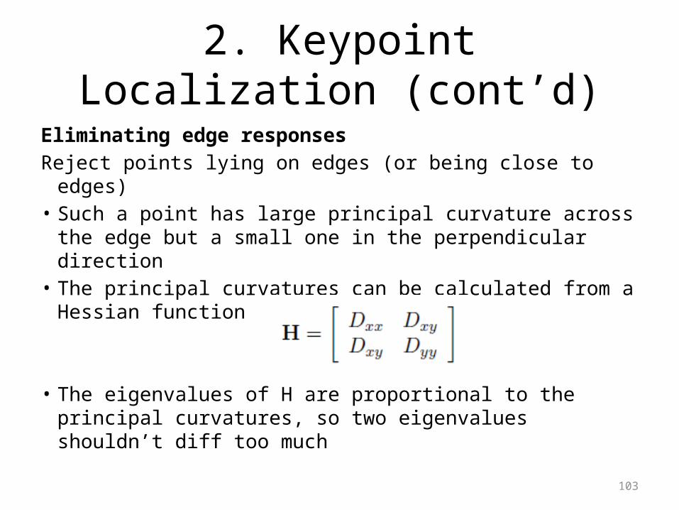
2. Keypoint Localization (cont’d)
Eliminating edge responsesReject points lying on edges (or being close to edges)• Such a point has large principal curvature across the
edge but a small one in the perpendicular direction• The principal curvatures can be calculated from a
Hessian function
• The eigenvalues of H are proportional to the principal curvatures, so two eigenvalues shouldn’t diff too much
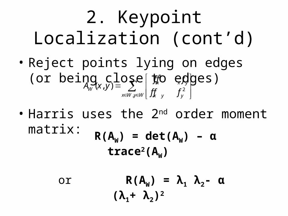
2. Keypoint Localization (cont’d)
• Reject points lying on edges (or being close to edges)
• Harris uses the 2nd order moment matrix:
2
2,
( , ) x x yW
x W y W x y y
f f fA x y
f f f
R(AW) = det(AW) – α trace2(AW)
or R(AW) = λ1 λ2- α (λ1+ λ2)2
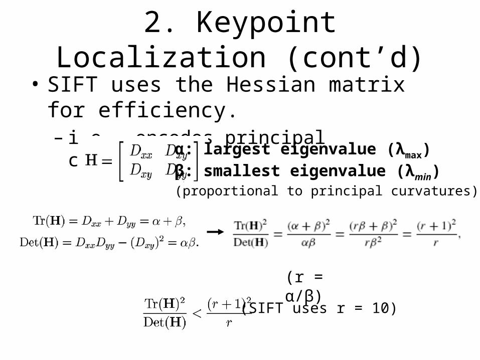
2. Keypoint Localization (cont’d)• SIFT uses the Hessian matrix for efficiency.
– i.e., encodes principal curvatures
α: largest eigenvalue (λmax)β: smallest eigenvalue (λmin)(proportional to principal curvatures)
(SIFT uses r = 10)
(r = α/β)
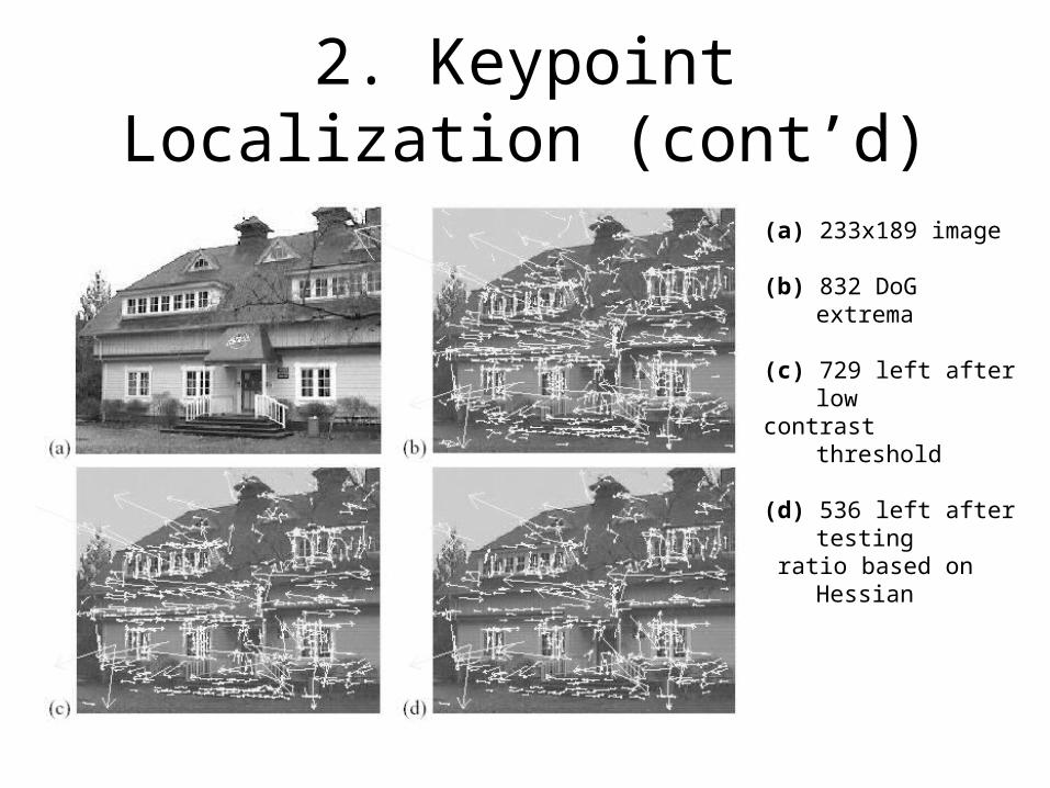
2. Keypoint Localization (cont’d)
(a) 233x189 image
(b) 832 DoG extrema
(c) 729 left after low contrast threshold
(d) 536 left after testing ratio based on Hessian
107
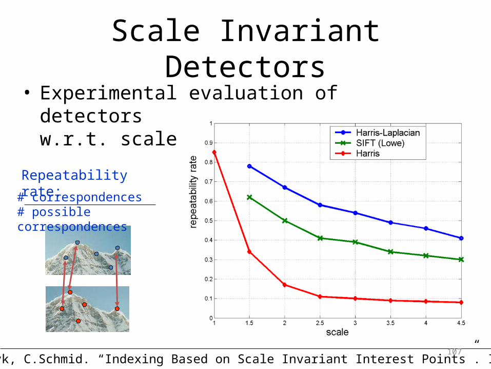
Scale Invariant Detectors
K.Mikolajczyk, C.Schmid. “Indexing Based on Scale Invariant Interest Points”. ICCV 2001
• Experimental evaluation of detectors w.r.t. scale change
Repeatability rate:
# correspondences# possible correspondences
108
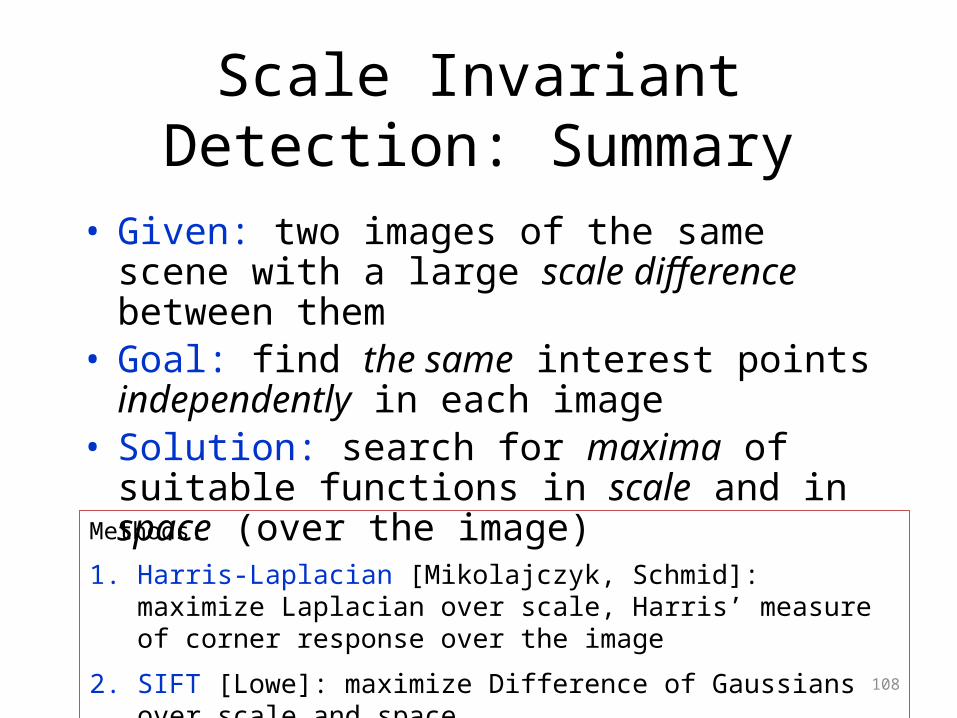
Scale Invariant Detection: Summary
• Given: two images of the same scene with a large scale difference between them
• Goal: find the same interest points independently in each image
• Solution: search for maxima of suitable functions in scale and in space (over the image)
Methods:
1. Harris-Laplacian [Mikolajczyk, Schmid]: maximize Laplacian over scale, Harris’ measure of corner response over the image
2. SIFT [Lowe]: maximize Difference of Gaussians over scale and space
109
Methods using invariant descriptors
• Local features– Feature Detector
• Point detector– Corner detectors
» Moravec, harris, – Low’s key point
– Feature descriptor• SIFT
– Feature-matching
Outline
Motivation
Problems statement
How we solve it
• Methods of Feature matching
• Invariant descriptors
Applications
Future Work
Conclusion
110
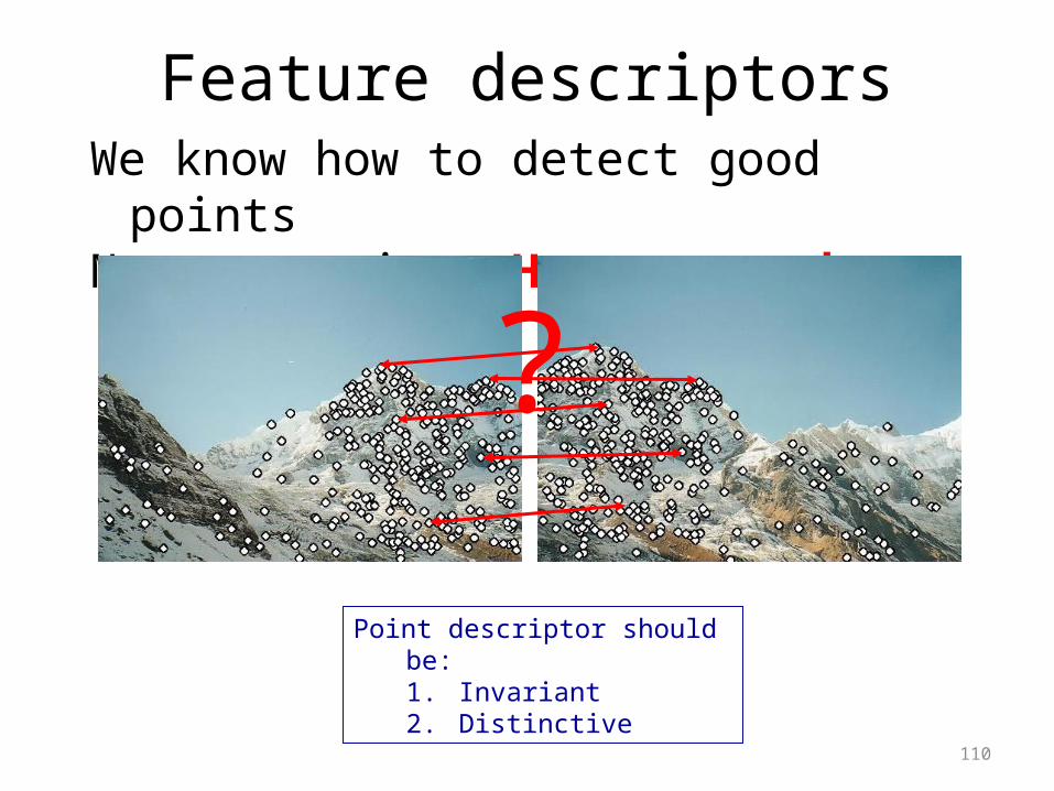
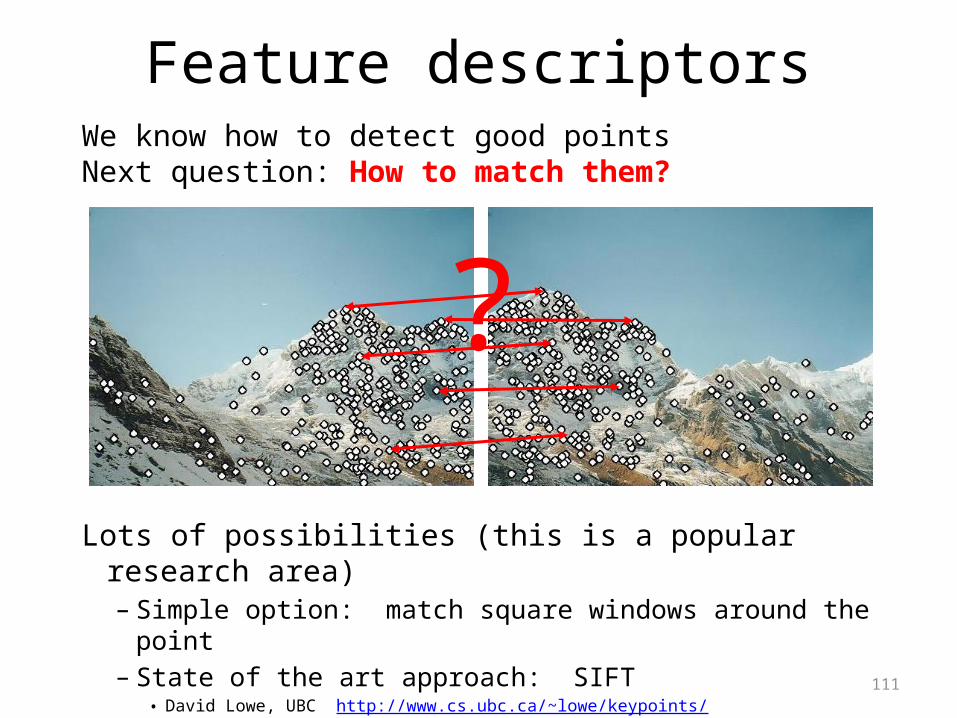
Feature descriptorsWe know how to detect good pointsNext question: How to match them?
?
Point descriptor should be:1. Invariant2. Distinctive
111
Feature descriptorsWe know how to detect good pointsNext question: How to match them?
Lots of possibilities (this is a popular research area)– Simple option: match square windows around the point– State of the art approach: SIFT
• David Lowe, UBC http://www.cs.ubc.ca/~lowe/keypoints/
?
Feature descriptors
112
N p
ixel
s
N pixels
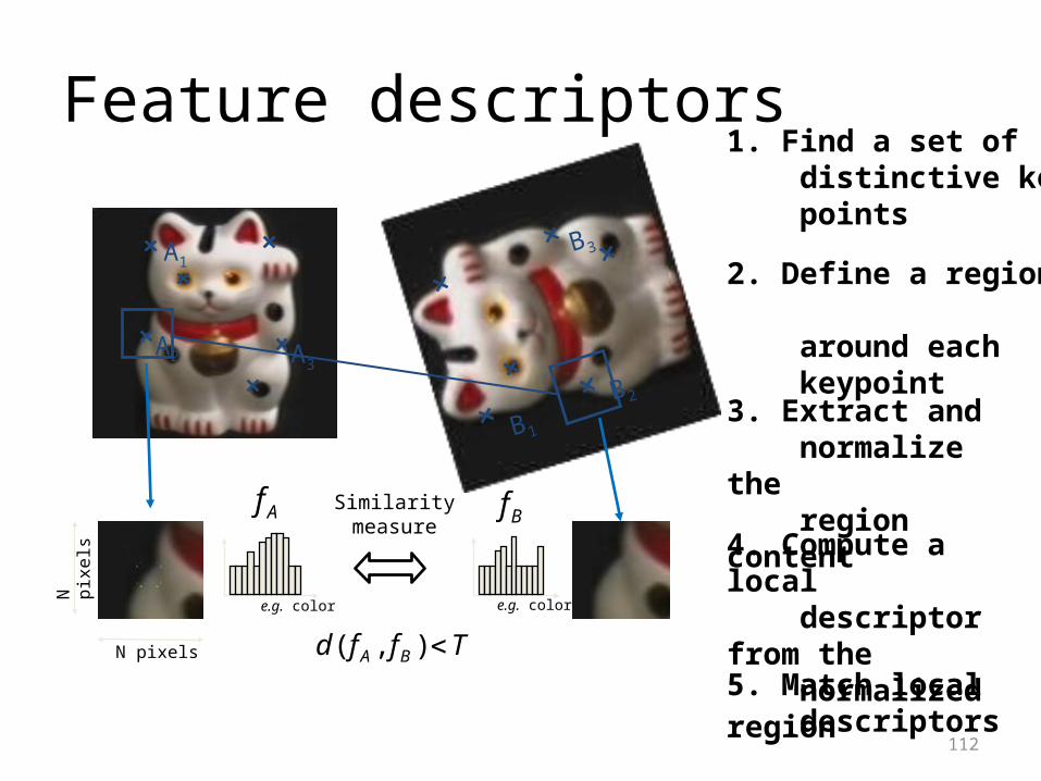
Similarity measureAf
e.g. color
Bf
e.g. color
B1
B2
B3A1
A2 A3
Tffd BA ),(
1. Find a set of distinctive key- points
3. Extract and normalize the region content
2. Define a region around each keypoint
4. Compute a local descriptor from the normalized region
5. Match local descriptors
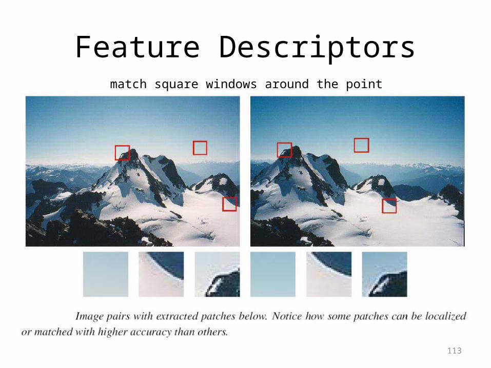
113
Feature Descriptorsmatch square windows around the point
114
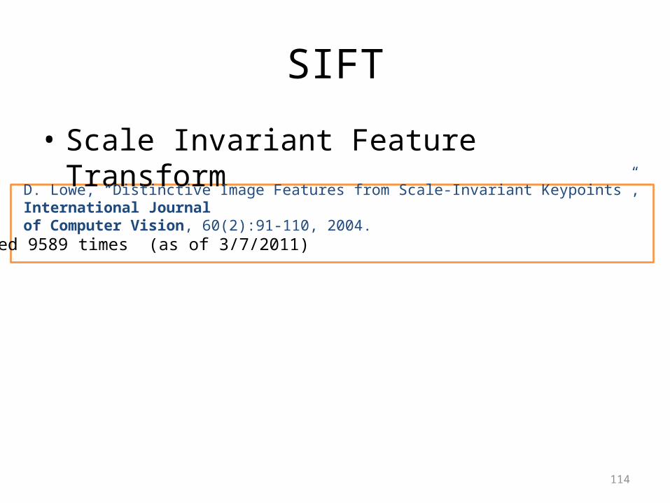
SIFT
• Scale Invariant Feature Transform
D. Lowe, “Distinctive Image Features from Scale-Invariant Keypoints”, International Journal of Computer Vision, 60(2):91-110, 2004.
Cited 9589 times (as of 3/7/2011)
115
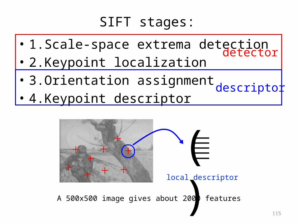
SIFT stages:
• 1.Scale-space extrema detection• 2.Keypoint localization• 3.Orientation assignment• 4.Keypoint descriptor
( )local descriptor
detector
descriptor
A 500x500 image gives about 2000 features
116
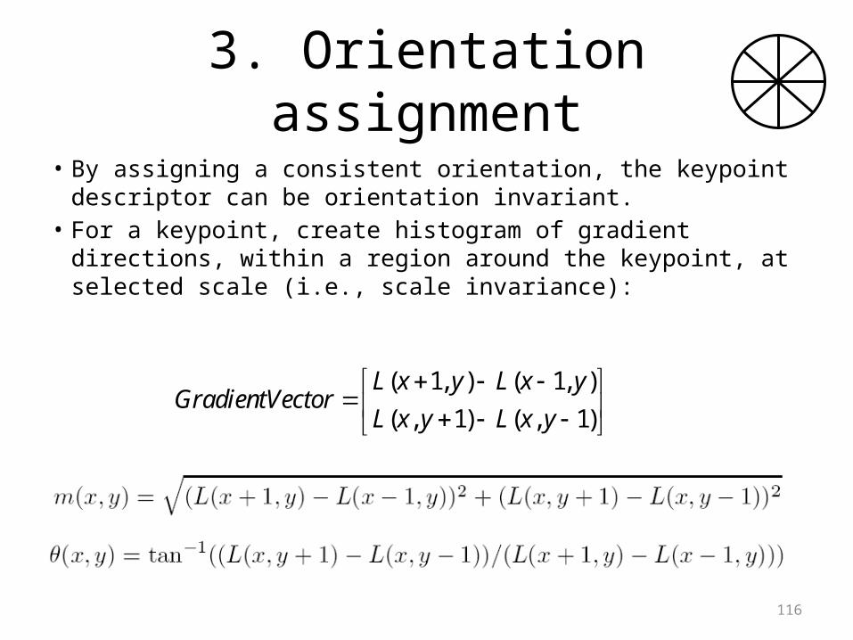
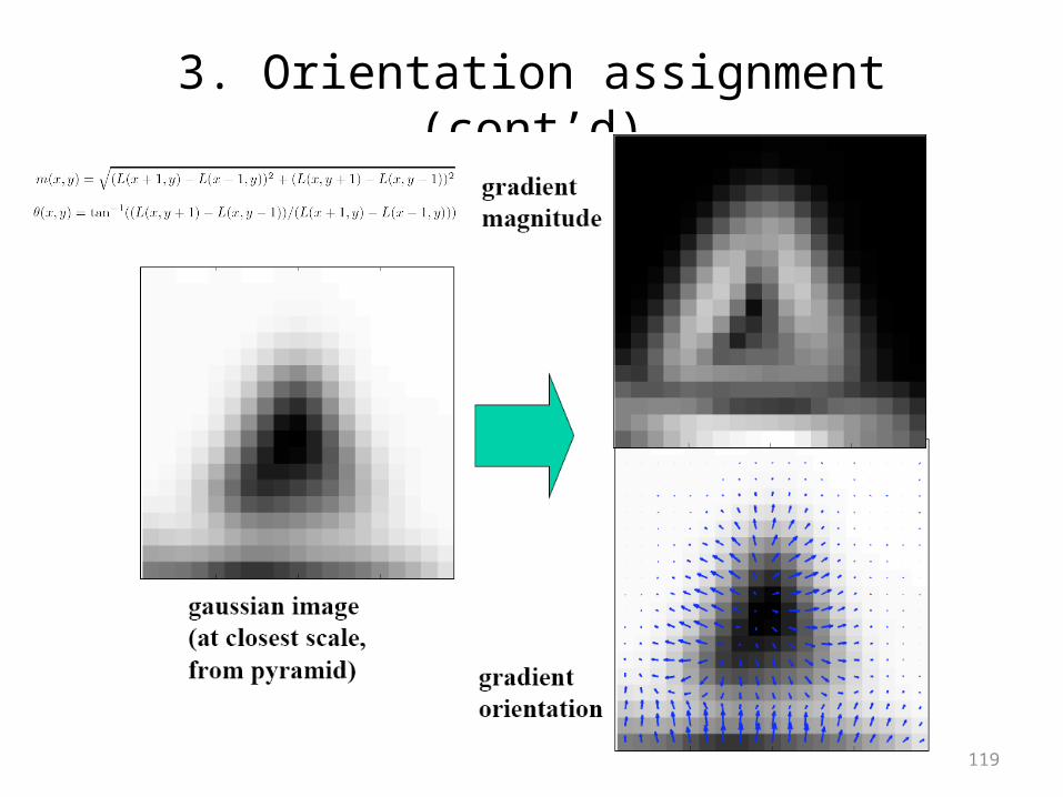
3. Orientation assignment
• By assigning a consistent orientation, the keypoint descriptor can be orientation invariant.
• For a keypoint, create histogram of gradient directions, within a region around the keypoint, at selected scale (i.e., scale invariance):
( 1, ) ( 1, )
( , 1) ( , 1)
L x y L x yGradientVector
L x y L x y
117
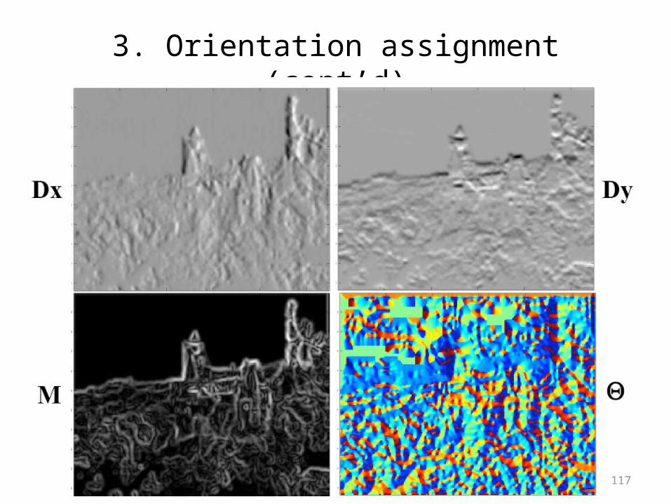
3. Orientation assignment (cont’d)
118
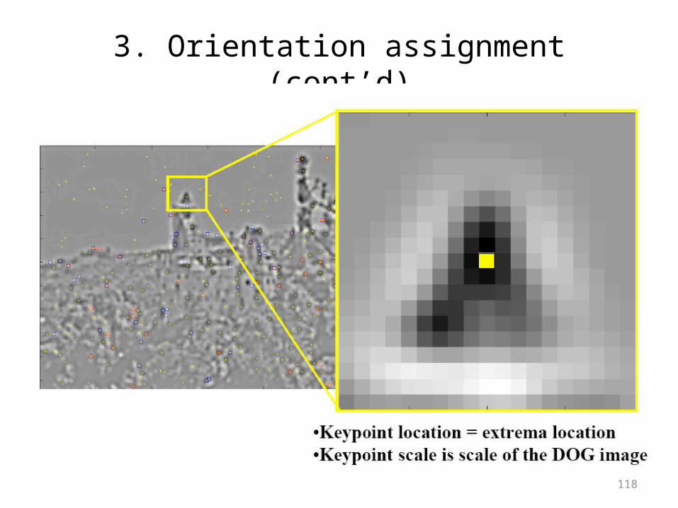
3. Orientation assignment (cont’d)
119
3. Orientation assignment (cont’d)
120
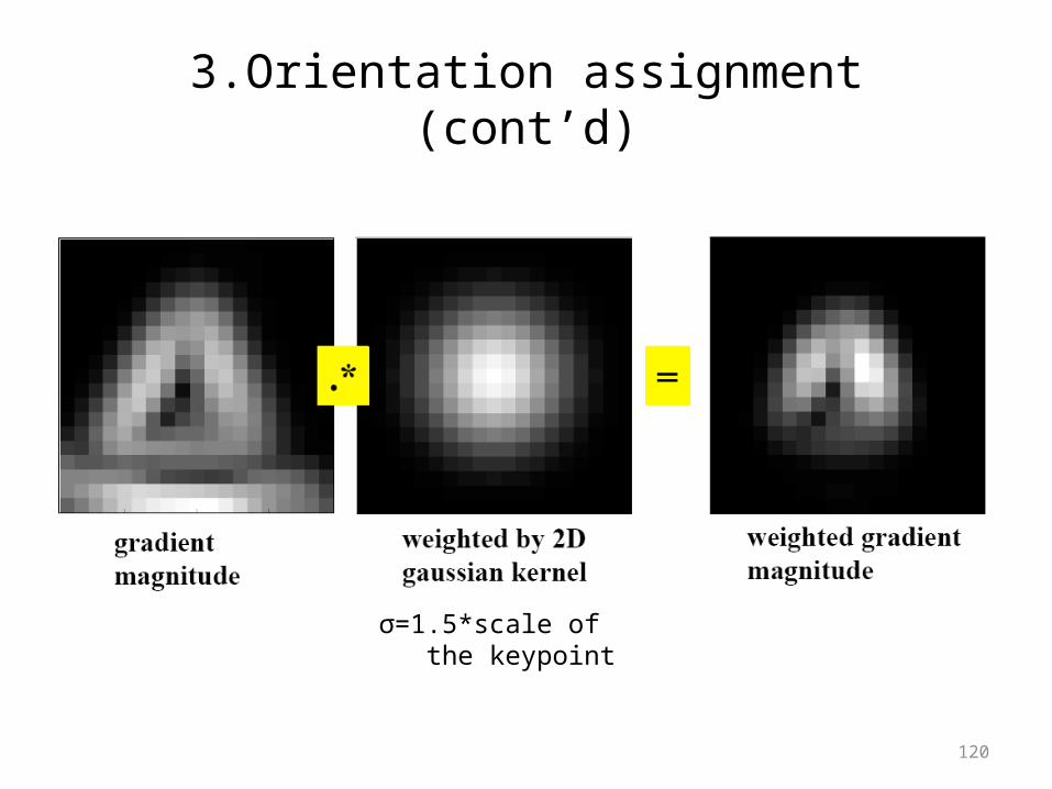
3.Orientation assignment (cont’d)
σ=1.5*scale of the keypoint
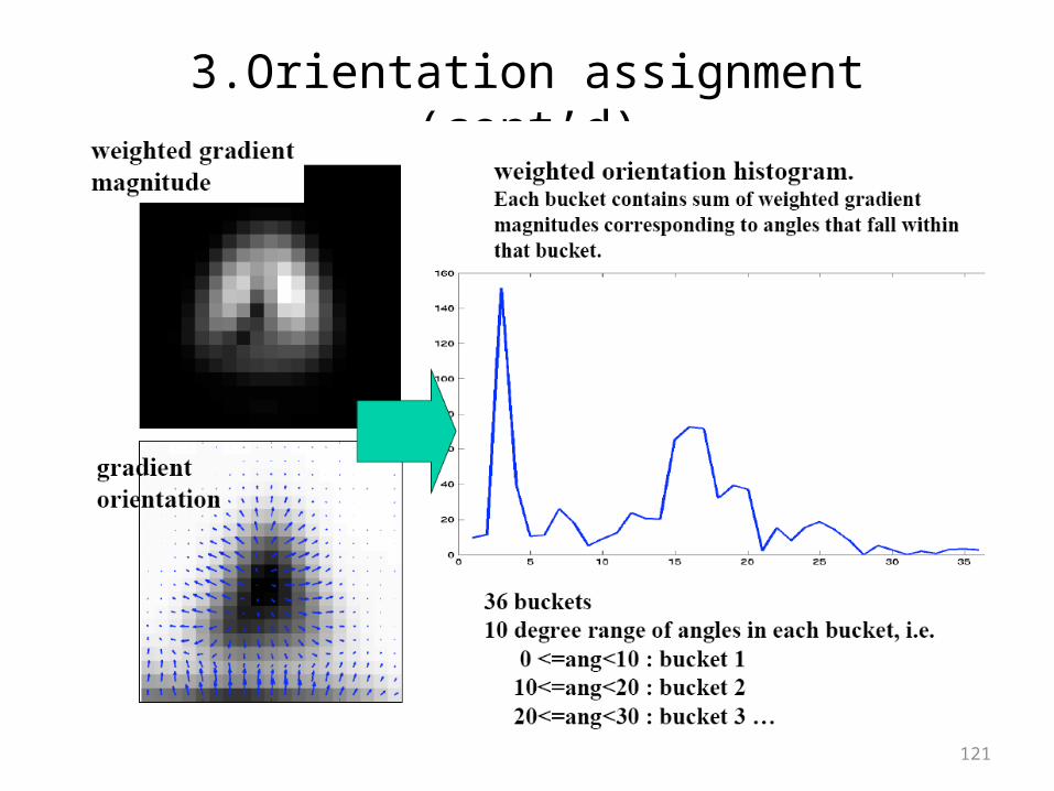
121
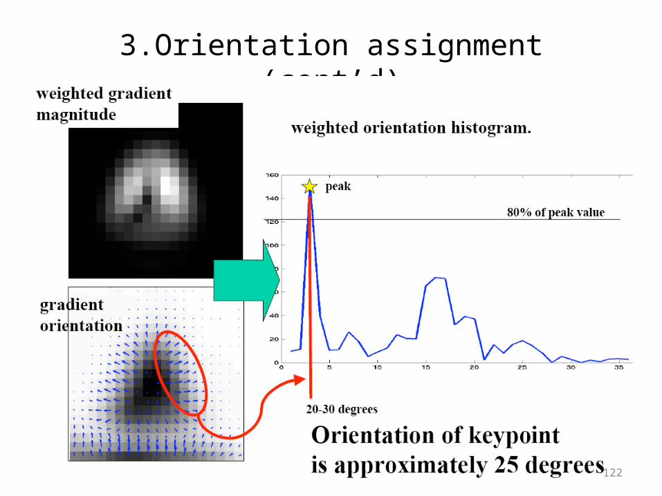
3.Orientation assignment (cont’d)
122
3.Orientation assignment (cont’d)
123
4. Keypoint Descriptor
• Have achieved invariance to location, scale, and orientation.
• Next, tolerate illumination and viewpoint changes.
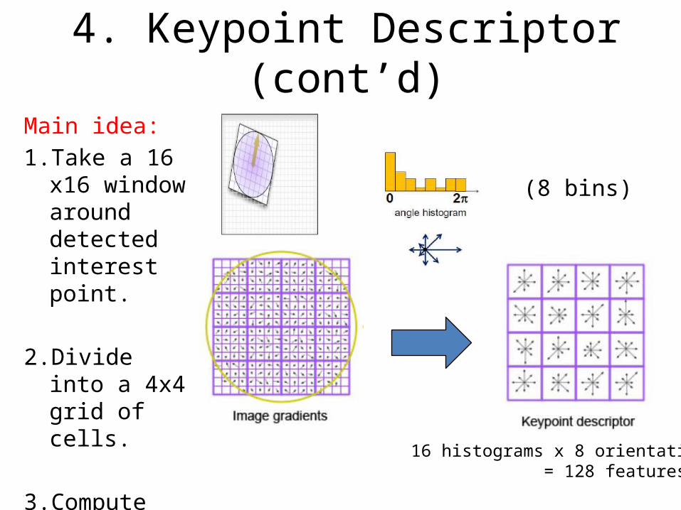
4. Keypoint Descriptor (cont’d)
16 histograms x 8 orientations = 128 features
Main idea:1. Take a 16 x16
window around detected interest point.
2. Divide into a 4x4 grid of cells.
3. Compute histogram in each cell.
(8 bins)
125
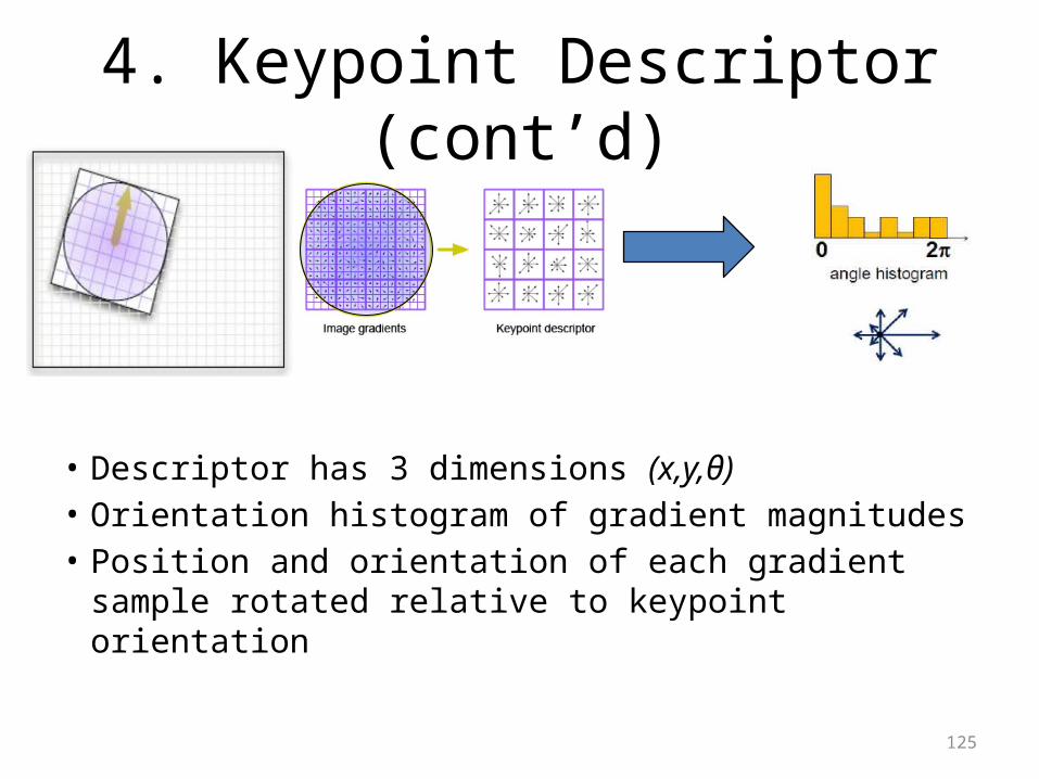
4. Keypoint Descriptor (cont’d)
• Descriptor has 3 dimensions (x,y,θ)• Orientation histogram of gradient magnitudes• Position and orientation of each gradient
sample rotated relative to keypoint orientation
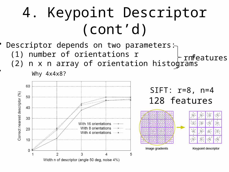
4. Keypoint Descriptor (cont’d)
128 features
• Descriptor depends on two parameters:(1) number of orientations r(2) n x n array of orientation histograms
•
SIFT: r=8, n=4
rn2 features
Why 4x4x8?
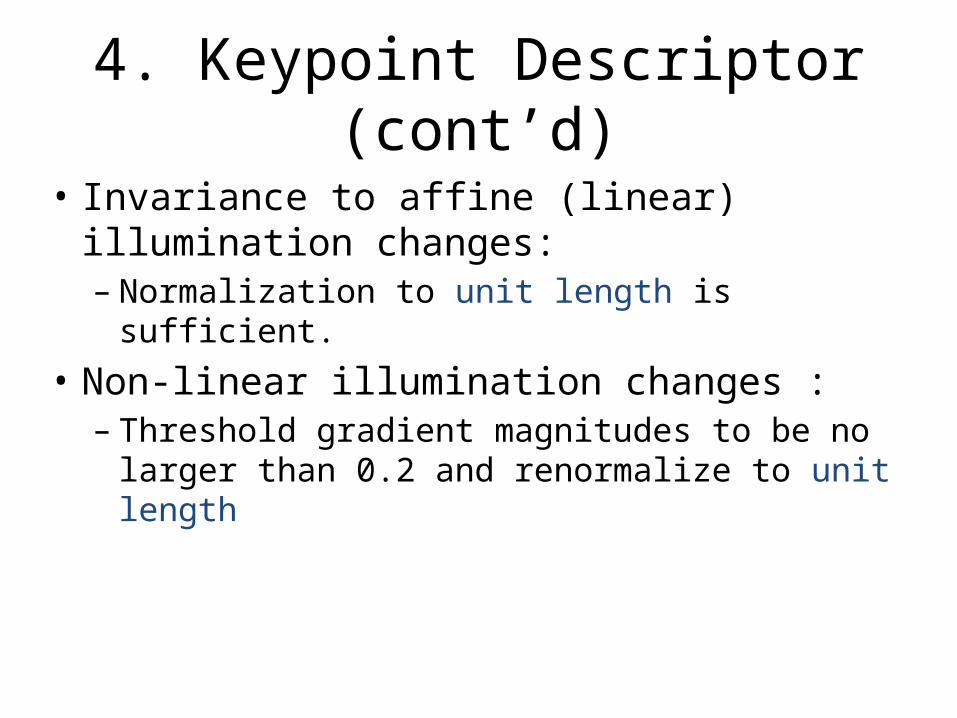
4. Keypoint Descriptor (cont’d)
• Invariance to affine (linear) illumination changes:– Normalization to unit length is sufficient.
• Non-linear illumination changes :– Threshold gradient magnitudes to be no larger
than 0.2 and renormalize to unit length
128
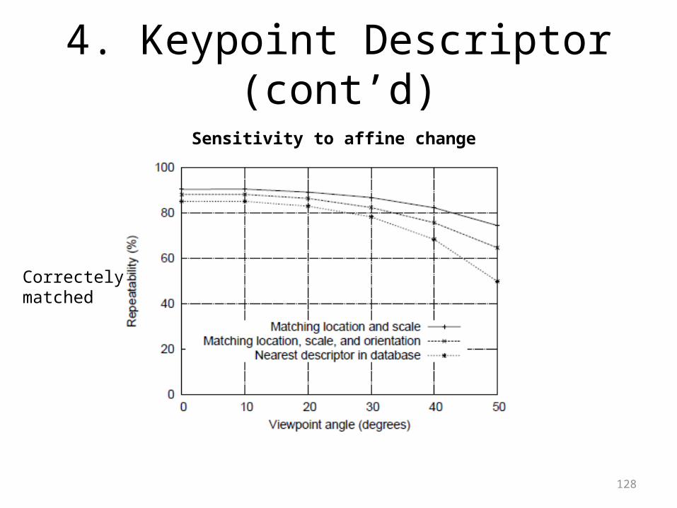
4. Keypoint Descriptor (cont’d)
Sensitivity to affine change
Correctely matched
129
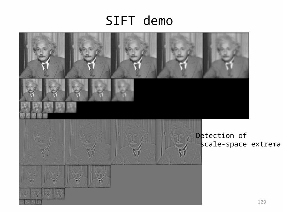
SIFT demo
Detection of scale-space extrema
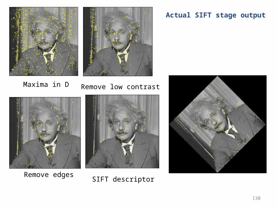
130
Maxima in D Remove low contrast
Remove edgesSIFT descriptor
Actual SIFT stage output
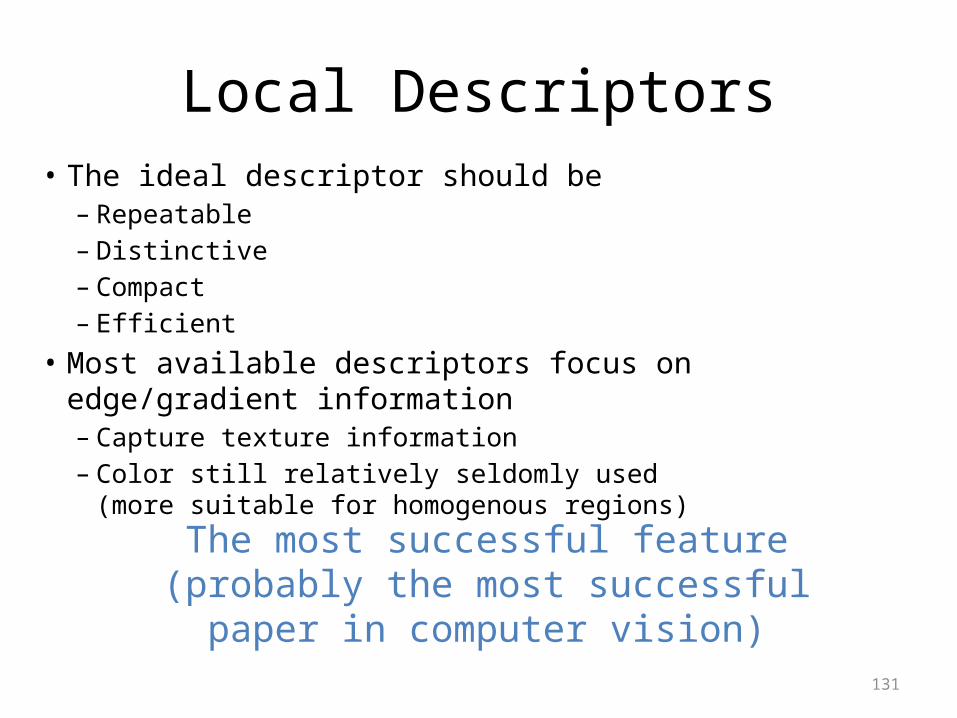
Local Descriptors• The ideal descriptor should be
– Repeatable– Distinctive– Compact– Efficient
• Most available descriptors focus on edge/gradient information– Capture texture information– Color still relatively seldomly used
(more suitable for homogenous regions)
131
The most successful feature (probably the most successful paper in computer vision)
Applications of SIFT
• Object recognition• Object categorization• Location recognition• Robot localization• Image retrieval• Image panoramas
133
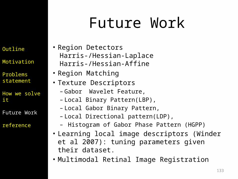
Future Work• Region Detectors
Harris-/Hessian-Laplace Harris-/Hessian-Affine
• Region Matching• Texture Descriptors
– Gabor Wavelet Feature, – Local Binary Pattern(LBP), – Local Gabor Binary Pattern, – Local Directional pattern(LDP),– Histogram of Gabor Phase Pattern (HGPP)
• Learning local image descriptors (Winder et al 2007): tuning parameters given their dataset.
• Multimodal Retinal Image Registration
Outline
Motivation
Problems statement
How we solve it
Future Work
reference
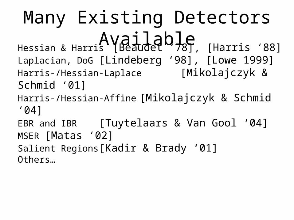
Many Existing Detectors AvailableHessian & Harris [Beaudet ‘78], [Harris ‘88]Laplacian, DoG [Lindeberg ‘98], [Lowe 1999]Harris-/Hessian-Laplace [Mikolajczyk & Schmid ‘01]Harris-/Hessian-Affine[Mikolajczyk & Schmid ‘04]EBR and IBR [Tuytelaars & Van Gool ‘04] MSER [Matas ‘02]Salient Regions [Kadir & Brady ‘01] Others…
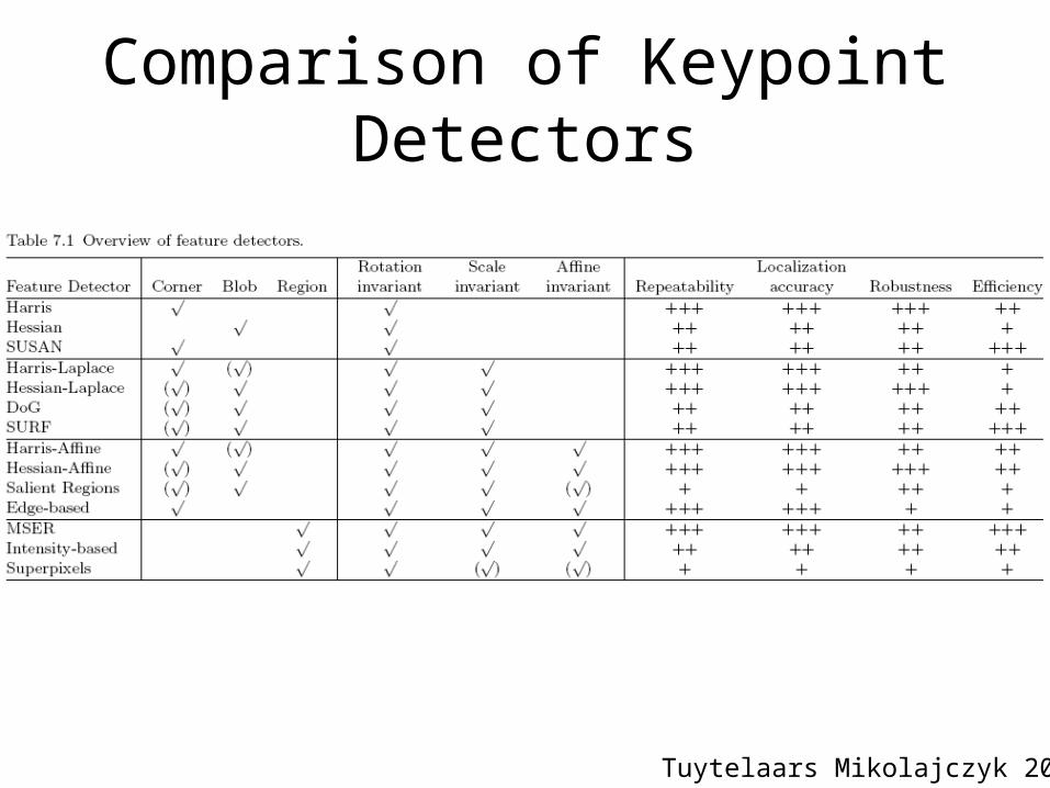
Comparison of Keypoint Detectors
Tuytelaars Mikolajczyk 2008
136
Reference
Outline
Motivation
Problems statement
How we solve it
Future Work
Reference
• Chris Harris, Mike Stephens, A Combined Corner and Edge Detector, 4th Alvey Vision Conference, 1988, pp147-151.
• David G. Lowe, Distinctive Image Features from Scale-Invariant Keypoints, International Journal of Computer Vision, 60(2), 2004, pp91-110.
• Yan Ke, Rahul Sukthankar, PCA-SIFT: A More Distinctive Representation for Local Image Descriptors, CVPR 2004.
• Krystian Mikolajczyk, Cordelia Schmid, A performance evaluation of local descriptors, Submitted to PAMI, 2004.
• SIFT Keypoint Detector, David Lowe.• Matlab SIFT Tutorial, University of Toronto.• “Local Invariant Feature Detectors: A Survey”, Tinne Tuytelaars and
Krystian Mikolajczyk, Computer Graphics and Vision, Vol. 3, No. 3 (2007) 177–280
137
Reference
• http://en.wikipedia.org/wiki/Scale-invariant_feature_transform
Outline
Motivation
Problems statement
How we solve it
Future Work
Reference