Embed Size (px)
Citation preview

Computer Vision, Convolutions, Complexityand Algebraic Geometry
D. V. Chudnovsky, G.V. ChudnovskyIMAS
Polytechnic Institute of NYU6 MetroTech CenterBrooklyn, NY 11201
December 6, 2012

Fast Multiplication: glimpse
Gauss 1801-1809Not dwarf planet Ceres, but an asteroid Pallas
(a0 + a1i) · (b0 + b1i) = a0 · b0 − a1 · b1 + (a0 · b1 + a1 · b0)i
instead
a0 · b0a1 · b1
(a0 + a1) · (b0 + b1)
(a0 + a1) · (b0 + b1)− (a0 · b0 + a1 · b1)
3 multiplies and 5 add/sub instead of 4 multiply and 2 add/sub.
Fast Multiplication: the beginning
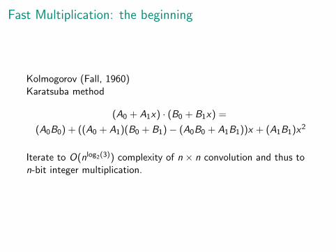
Kolmogorov (Fall, 1960)Karatsuba method
(A0 + A1x) · (B0 + B1x) =
(A0B0) + ((A0 + A1)(B0 + B1)− (A0B0 + A1B1))x + (A1B1)x2
Iterate to O(nlog2(3)) complexity of n × n convolution and thus ton-bit integer multiplication.

Polynomials and Interpolation
Karatsuba method as evaluation/interpolation at x = 0, 1,∞.Toom(-Cook) method
Multiply P(x) = a0 + · · ·+ an−1xn−1 and
Q(x) = b0 + · · ·+ bm−1xm−1 using interpolation of the polynomial
P(x) · Q(x) at n +m − 1 points x = 0, 1, . . . , n +m − 2.
Leads to n+m− 1 multiplication of linear forms in ai , bj but theselinear forms have rational coefficients of the height O(nn).
Early papers on fast convolution
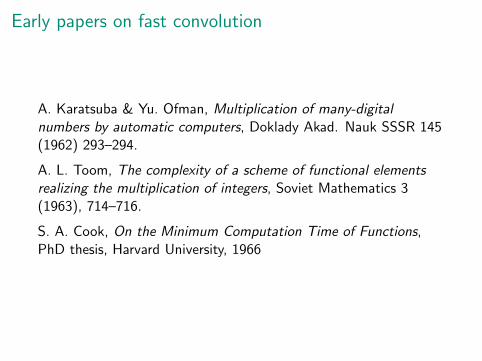
A. Karatsuba & Yu. Ofman, Multiplication of many-digitalnumbers by automatic computers, Doklady Akad. Nauk SSSR 145(1962) 293–294.
A. L. Toom, The complexity of a scheme of functional elementsrealizing the multiplication of integers, Soviet Mathematics 3(1963), 714–716.
S. A. Cook, On the Minimum Computation Time of Functions,PhD thesis, Harvard University, 1966

Bilinear Forms and Multiplicative Complexity
Strassen (1969) 7 for 8
Bilinear forms in variables x0, . . . , xn−1 and y0, . . . , ym−1
zk =n−1∑
i=0
m−1∑
j=0
Ti ,j ,k · xi · yj : k = 1, . . . , s
over some algebra A (typically a field F).
The (multiplicative) complexity of computation of these forms overA, µA(T ) is the rank of the tensor T over A.

Bilinear Forms and Multiplicative Complexity (cont.)
Here rank 1 tensor is just like rank 1 matrix:
Ti ,j ,k = ai · bj · ckfor scalars ai , bj , ck from A.
The tensor T has a rank µ if it is the sum of µ (and not less) ofrank 1 tensors. This defines the multiplicative complexity of Tover A:
µ = µA(T )
In the matrix form, we have A,B ,C matrices (fromMµ,n(A),Mµ,m(A),Ms,µ(A)) such that:
~z = C · (A~x ⊗ B~y)
Complexity of one-dimensional convolution over infinitefields
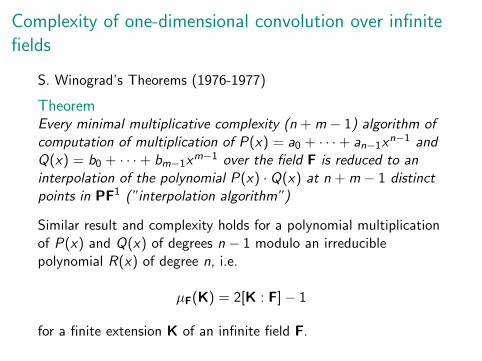
S. Winograd’s Theorems (1976-1977)
TheoremEvery minimal multiplicative complexity (n +m − 1) algorithm ofcomputation of multiplication of P(x) = a0 + · · ·+ an−1x
n−1 andQ(x) = b0 + · · ·+ bm−1x
m−1 over the field F is reduced to aninterpolation of the polynomial P(x) · Q(x) at n +m − 1 distinctpoints in PF1 (”interpolation algorithm”)
Similar result and complexity holds for a polynomial multiplicationof P(x) and Q(x) of degrees n − 1 modulo an irreduciblepolynomial R(x) of degree n, i.e.
µF(K) = 2[K : F]− 1
for a finite extension K of an infinite field F.
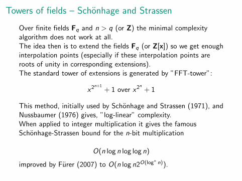
Towers of fields – Schonhage and Strassen
Over finite fields Fq and n > q (or Z) the minimal complexityalgorithm does not work at all.The idea then is to extend the fields Fq (or Z[x]) so we get enoughinterpolation points (especially if these interpolation points areroots of unity in corresponding extensions).The standard tower of extensions is generated by ”FFT-tower”:
x2n+1
+ 1 over x2n
+ 1
This method, initially used by Schonhage and Strassen (1971), andNussbaumer (1976) gives, ”log-linear” complexity.When applied to integer multiplication it gives the famousSchonhage-Strassen bound for the n-bit multiplication
O(n log n log log n)
improved by Furer (2007) to O(n log n2O(log∗ n)).
Papers on complexity of bilinear forms
V. Strassen, Gaussian elimination is not optimal, Numer. Math. 13(1969) 354–356. 5–685.
S. Winograd, Some bilinear forms whose multiplicative complexitydepends on the field of constants, Math. Systems Theory 10(1977) 169–180.
C. Fiduccia & Y. Zalcstein, Algebras having linear multiplicativecomplexities, J. Assoc. Comput. Mach. 24 (1977) 311–331.
V. Strassen, Rank and optimal computation of generic tensors,Linear Algebra Appl. 52/53 (1983) 64
H. F. de Groote, Lectures on the complexity of bilinear problems,Lecture Notes in Comp. Science 245, Springer-Verlag, 1987.

Linear Codes from Multiplication Algorithms
When the tensor
T = Ti ,j ,k i , j , k = 1, . . . n
defines the multiplication in the (n-dimensional) algebra A over thefinite field Fq, any of its representation as a sum of rank 1 tensorsgives rise to q-ary linear codes with special distance properties.
For example, if the algebra A has no divisors of 0, then all threeµ× n matrices A,B ,CT are generators of q-ary linear codes oflength µ = µFq
(A) and the dimension n with the minimal weight(distance) of n.
Moreover, three codes, generated by A,B ,CT are intersecting, i.e.any code vectors from any two of these codes have non-emptycommon support.

Linear Codes and Better Lower Bounds
Applying Elias bound to binary codes, we get the lower bound formultiplication complexity:
µF2(F2n) ≥ 3.5275.. · nIn particular, a weak corollary:
µF2(n × n) ≥ 3.5275.. · nIn general, multiplication of polynomials of degree n modulo anypolynomial of degree ≥ n over Fq has a multiplicative complexity
µFq≥ (2 +
1
q − 1) · n − o(n)
Hankel matrices..

Interpolate on Algebraic Curves of genus g > 0
In 1986 we needed better algorithms of integer multiplications, i.e.faster convolutions over Z, or Z[12 ], Z[
13 ], etc. – start with finite
fields.
Do all minimal complexity convolution algorithms come frominterpolations on algebraic surfaces?
Needed curves with many points over finite fields.Ihara (1981) proved first results for modular curves.
Nq(g) = max{|X (Fq)| : X is a curve of genus g over Fq}
A−(q) = lim infg→∞Nq(g)
g
A+(q) = lim supg→∞Nq(g)
g
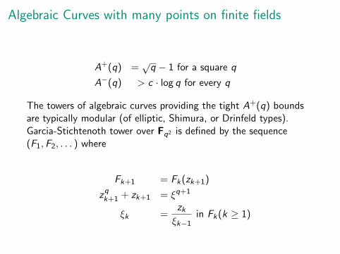
Algebraic Curves with many points on finite fields
A+(q) =√q − 1 for a square q
A−(q) > c · log q for every q
The towers of algebraic curves providing the tight A+(q) boundsare typically modular (of elliptic, Shimura, or Drinfeld types).Garcia-Stichtenoth tower over Fq2 is defined by the sequence(F1,F2, . . . ) where
Fk+1 = Fk(zk+1)
zqk+1 + zk+1 = ξq+1
ξk =zkξk−1
in Fk(k ≥ 1)
Our papers and a general review
D. V. & G. V. Chudnovsky, Algebraic complexities and algebraiccurves over finite fields, Proc. Nat. Acad. Sci. USA 84 (1987)1739–1743.
D. V. & G. V. Chudnovsky, Algebraic complexities and algebraiccurves over finite fields, J. Complexity 4 (1988) 285–316.
P. Burgisser, M. Clausen & A. Shokrollahi, Algebraic complexitytheory, Grundlehren der Math. Wissenschaften 315,Springer-Verlag, 1997.
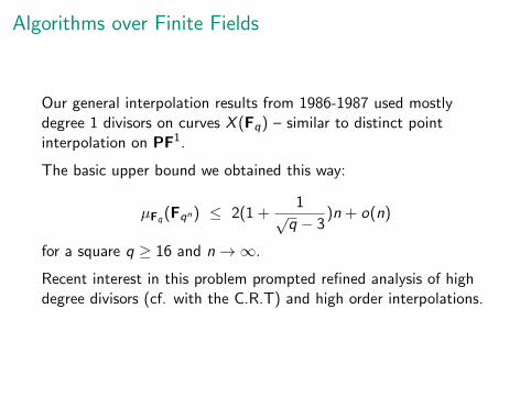
Algorithms over Finite Fields
Our general interpolation results from 1986-1987 used mostlydegree 1 divisors on curves X (Fq) – similar to distinct pointinterpolation on PF1.
The basic upper bound we obtained this way:
µFq(Fqn) ≤ 2(1 +
1√q − 3
)n + o(n)
for a square q ≥ 16 and n → ∞.
Recent interest in this problem prompted refined analysis of highdegree divisors (cf. with the C.R.T) and high order interpolations.

Improved upper bounds
The recent series of results show (after corrections..) a slightlybetter bound:
µFq(Fqn) ≤ 2(1 +
1√q − 2
)n + o(n)
for a square q ≥ 9 and sufficiently large n.
The original 1987 bound as well as these improved ones give ageneral linear bound for a one-dimensional convolution:
µFq(n × n) ≤ Cq · n
The upper bound on Cq (for a square q ≥ 9) is 4(1 + 1√q−2), and a
low bound is 3 + ǫ(q), for any q. E.g. for q = 3 the low bound is3.005.

Recent papers on convolutions and algebraic geometry
Hugues Randriambololona, Bilinear complexity of algebras and theChudnovsky–Chudnovsky interpolation method Journal ofComplexity 28 (2012) 489–517
S. Ballet, On the tensor rank of the multiplication in the finitefields, J. Number Theory 128 (2008) 1795–1806.
S. Ballet, D. Le Brigand & R. Rolland, “On an application of thedefinition field descent of a tower of function fields”, in: F. Rodier& S. Vladut (eds.), Proceedings of the Conference ”Arithmetic,Geometry and Coding Theory” (AGCT 2005), Seminaires etCongres 21, Societe Mathematique de France, 2010, pp. 187–203.
S. Ballet & J. Pieltant, On the tensor rank of multiplication in anyextension of F2, J. Complexity 27 (2011) 230–245.
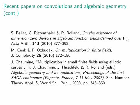
Recent papers on convolutions and algebraic geometry(cont.)
S. Ballet, C. Ritzenthaler & R. Rolland, On the existence ofdimension zero divisors in algebraic function fields defined over Fq,Acta Arith. 143 (2010) 377–392.
M. Cenk & F. Ozbudak, On multiplication in finite fields,J. Complexity 26 (2010) 172–186.
J. Chaumine, “Multiplication in small finite fields using ellipticcurves”, in: J. Chaumine, J. Hirschfeld & R. Rolland (eds.),Algebraic geometry and its applications, Proceedings of the firstSAGA conference (Papeete, France, 7-11 May 2007), Ser. NumberTheory Appl. 5, World Sci. Publ., 2008, pp. 343–350.

Bounds for One-Dimensional Convolutions over F3 – part 1
Convolution Complexity Lower Bound method Upper Bound Method
2× 2 µF3(2× 2) = 3 Dimensions Standard (Karatsuba)
3× 2 µF3(3× 2) = 4 Dimensions Standard (Toom-Cook)
3× 3 µF3(3× 3) = 6 Codes C.R.T
4× 2 µF3(4× 2) = 6 Codes C.R.T
4× 3 µF3(4× 3) = 7 Exhaustive C.R.T
4× 4 µF3(4× 4) = 9 Codes C.R.T
5× 2 µF3(5× 2) = 7 Exhaustive C.R.T
5× 3 µF3(5× 3) = 9 Hankel matrices C.R.T
5× 4 µF3(5× 4) = 10 Hankel matrices C.R.T
5× 5 µF3(5× 5) = 12 Hankel matrices C.R.T
6× 2 µF3(6× 2) = 8 Codes C.R.T
6× 3 µF3(6× 3) = 10 Hankel matrices C.R.T
6× 4 µF3(6× 4) = 12 Hankel matrices (New) C.R.T
6× 5 µF3(6× 5) = 13 Hankel matrices (New) C.R.T
6× 6 µF3(6× 6) = 15 Hankel matrices (New) Field Extension
7× 2 µF3(7× 2) = 10 Codes C.R.T
7× 3 µF3(7× 3) = 12 Hankel matrices (New) C.R.T
7× 4 µF3(7× 4) = 13 Hankel matrices (New) C.R.T
7× 7 18 ≤ µF3(7× 7) ≤ 19 Hankel matrices (New) C.R.T
8× 2 µF3(8× 2) = 11 Codes C.R.T
8× 3 µF3(8× 3) = 13 Hankel matrices (New) C.R.T
8× 8 19 ≤ µF3(8× 8) ≤ 23 Hankel matrices (New) Field Extension

Bounds for One-Dimensional Convolutions – part 2Some new (mostly low bound) special interesting cases; a single new type of upperbound algorithm (6 non-equivalent solutions)
Convolution Complexity Lower Bound Upper/State
6× 5 15 ≤ µF2(6× 5) ≤ 16 1D Hankel Upper Bound C.R.T.
6× 6 µF2(6× 6) = 17 1D Hankel Open since 1987
7× 7 19 ≤ µF2(7× 7) ≤ 22 1D Hankel Upper Bound C.R.T.
F27 18 ≤ µF2(F27) ≤ 22 1D Hankel Upper Bound C.R.T.
mod (Q2(x)2, 3) µF3(Q2(x)
2) = 9 Codes New: Open since 1987
In the last case A = B arise from ternary code generator matrix defining the algebrawith 0 divisors up to the isotopy
1 0 0 0 0 1 1 10 1 0 0 1 0 1 10 0 1 0 1 1 0 20 0 0 1 1 1 2 0
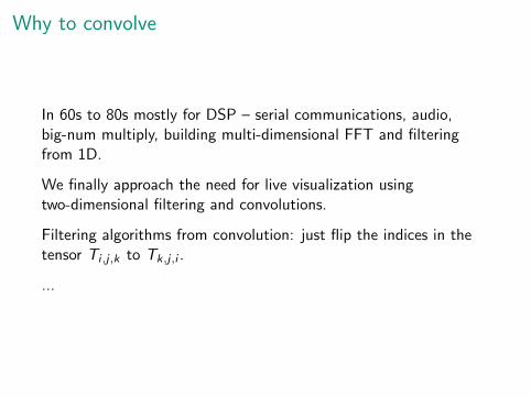
Why to convolve
In 60s to 80s mostly for DSP – serial communications, audio,big-num multiply, building multi-dimensional FFT and filteringfrom 1D.
We finally approach the need for live visualization usingtwo-dimensional filtering and convolutions.
Filtering algorithms from convolution: just flip the indices in thetensor Ti ,j ,k to Tk,j ,i .
...
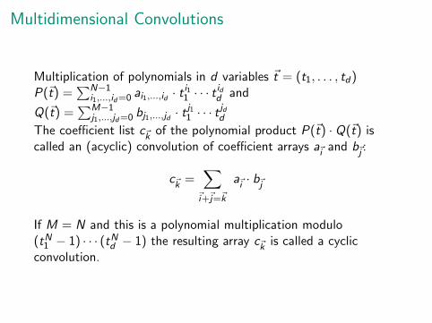
Multidimensional Convolutions
Multiplication of polynomials in d variables ~t = (t1, . . . , td)P(~t) =
∑N−1i1,...,id=0 ai1,...,id · t i11 · · · t idd and
Q(~t) =∑M−1
j1,...,jd=0 bj1,...,jd · tj11 · · · t jdd
The coefficient list c~k of the polynomial product P(~t) · Q(~t) iscalled an (acyclic) convolution of coefficient arrays a~i and b~j :
c~k =∑
~i+~j=~k
a~i · b~j
If M = N and this is a polynomial multiplication modulo(tN1 − 1) · · · (tNd − 1) the resulting array c~k is called a cyclicconvolution.
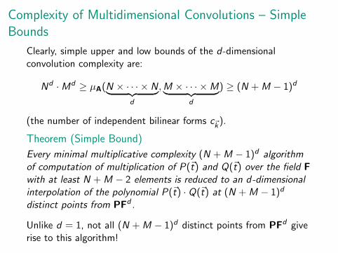
Complexity of Multidimensional Convolutions – SimpleBounds
Clearly, simple upper and low bounds of the d-dimensionalconvolution complexity are:
Nd ·Md ≥ µA(N × · · · × N︸ ︷︷ ︸
d
,M × · · · ×M︸ ︷︷ ︸
d
) ≥ (N +M − 1)d
(the number of independent bilinear forms c~k).
Theorem (Simple Bound)
Every minimal multiplicative complexity (N +M − 1)d algorithmof computation of multiplication of P(~t) and Q(~t) over the field Fwith at least N +M − 2 elements is reduced to an d-dimensionalinterpolation of the polynomial P(~t) · Q(~t) at (N +M − 1)d
distinct points from PFd .
Unlike d = 1, not all (N +M − 1)d distinct points from PFd giverise to this algorithm!

2D Hankel matrices
The complexity bounds in the 2-dimensional case can be obtainedusing the 2D Hankel matrices (”Hankel-block-Hankel”) having theform
H2 = (h~i+~j)(N−1)d ,(M−1)d
~i ,~j=~0
over finite fields Fq.
Not much is known – study of two-dimensional recurrences overfinite fields.
What is the number of 2D Hankel matrices of rank r? Is it afunction of q only, when r is less than min((N − 1)d , (M − 1)d)?

Better Bounds – can curves (surfaces) help us
Only a few examples with useful interpolation on surfaces.Still, one can get linear upper bounds (with respect to the minimalcomplexity = number of terms).
For this reduce d-dimensional polynomial multiplication to aone-dimensional one using a ”Kronecker trick” – a substitution of ad-dimensional monomial by a one-dimensional ”sparse” monomial.
t i11 · · · t idd → t i1+(2N−1)i2+···+(2N−1)d−1id
This allows us to get a far from optimal, but still a linear bound,on the complexity of the d-dimensional convolution:

Better Bounds – curves can help us
µA(N × · · · × N︸ ︷︷ ︸
d
,M × · · · ×M︸ ︷︷ ︸
d
) ≤ Cq · (2N − 1)d
where Cq is our linear factor for the 1D convolution bound;somewhere between 3 + ǫ(q) and 4 + δ(q), for ǫ, δ > 0 (→ 0 asq → ∞).
This bound is far from tight – sparse polynomial multiplication isused here.
What about peculiar Weierstrass gaps – short intervals repeated inarithmetic progressions (like 3, 4, 8, 9 in the 3× 3 by 3× 3 filters).

Practical cases of 2D ConvolutionsNew results; especially for lower bounds.
2D Convolution Complexity Lower Bound method
2× 2 by 2× 2 µF2(2× 2, 2× 2) = 9 Dimensions
3× 2 by 2× 2 µF2(3× 2, 2× 2) = 15 2D Hankel
3× 2 by 3× 2 µF2(3× 2, 3× 2) = 18 2D Hankel
3× 2 by 2× 3 19 ≤ µF2(3× 2, 2× 3) ≤ 22 2D Hankel
2× 2 by 3× 3 19 ≤ µF2(2× 2, 3× 3) ≤ 22 2D Hankel
4× 2 by 2× 2 µF2(4× 2, 2× 2) = 18 2D Hankel
3× 3 by 3× 3 29 ≤ µF2(3× 3, 3× 3) ≤ 33 2D Hankel
4× 2 by 3× 2 21 ≤ µF2(4× 2, 3× 2) ≤ 24 2D Hankel
4× 2 by 2× 3 23 ≤ µF2(4× 2, 2× 3) ≤ 27 2D Hankel
Not much chance for a tight 8× 8 by 8× 8 bound.

But what is the size and power...

Wires...