The Design of Calamari: an Ad-hoc Localization System for Sensor Networks

by Cameron Dean Whitehouse

Research Project

Submitted to the Department of Electrical Engineering and Computer Sciences, University of Cal-ifornia at Berkeley, in partial satisfaction of the requirements for the degree ofMaster of Science,Plan II.

Approval for the Report and Comprehensive Examination:

Committee:

David Culler, Research Adviser Date

Kristofer Pister, Second Reader Date

Fall 2002

The Design of Calamari: an Ad-hoc Localization System for Sensor Networks

Copyright Fall 2002

by

Cameron Dean Whitehouse

i

Abstract

The Design of Calamari: an Ad-hoc Localization System for Sensor Networks

by

Cameron Dean Whitehouse

Master of Science in Electrical Engineering and Computer Science

University of California at Berkeley

Professor David Culler, Research Advisor

This thesis describes the design of an ad-hoc localization system for sensor networks. We

begin by formulating design principles from a concrete implementation of a sensor network applica-

tion that requires localization. We show why several existing localization systems are unsatisfactory

for this application domain and propose a new system calledCalamari that is designed specifically

for this domain’s goals and constraints. We motivate and explain the design decisions pertinent to

Calamari’s ranging technology, calibration and localization algorithm. The ranging technologies

ultimately used are extremely cheap and simple and have approximately 30% error after simple

calibration. A new calibration procedure is designed that reduces this error to about 10%. A mod-

ificiation to APS, an existing distributed localization algorithm, is proposed that improves error by

20% to 30%. Preliminary experiments show that this ranging error with this algorithm is suffi-

cient to give rise to position estimates that are on average 20% of the maximum distance between

connected nodes in the network.

iii

Contents

List of Figures iv1 Introduction . . . . . . . . . . . . . . . . . . . . . . . . . . . . . . . . . . . . . . 12 A Motivating Application . . . . . . . . . . . . . . . . . . . . . . . . . . . . . . . 23 Design Principles . . . . . . . . . . . . . . . . . . . . . . . . . . . . . . . . . . . 4

3.1 Node-level Resolution . . . . . . . . . . . . . . . . . . . . . . . . . . . . 43.2 Scalable Deployment . . . . . . . . . . . . . . . . . . . . . . . . . . . . . 43.3 Event-driven . . . . . . . . . . . . . . . . . . . . . . . . . . . . . . . . . 53.4 Simple and Approximate Operation . . . . . . . . . . . . . . . . . . . . . 5

4 Existing Localization Systems . . . . . . . . . . . . . . . . . . . . . . . . . . . . 54.1 GPS . . . . . . . . . . . . . . . . . . . . . . . . . . . . . . . . . . . . . . 64.2 Cricket . . . . . . . . . . . . . . . . . . . . . . . . . . . . . . . . . . . . 64.3 AHLoS . . . . . . . . . . . . . . . . . . . . . . . . . . . . . . . . . . . . 74.4 Millibots . . . . . . . . . . . . . . . . . . . . . . . . . . . . . . . . . . . 7

5 Calamari Overview . . . . . . . . . . . . . . . . . . . . . . . . . . . . . . . . . . 86 The Ranging Technology . . . . . . . . . . . . . . . . . . . . . . . . . . . . . . . 9

6.1 Radio Connectivity and Hop-based Measures . . . . . . . . . . . . . . . . 106.2 Radio Signal Strength . . . . . . . . . . . . . . . . . . . . . . . . . . . . 136.3 Acoustic Time of Flight . . . . . . . . . . . . . . . . . . . . . . . . . . . 19

7 Calibration . . . . . . . . . . . . . . . . . . . . . . . . . . . . . . . . . . . . . . 267.1 Traditional Calibration . . . . . . . . . . . . . . . . . . . . . . . . . . . . 277.2 Calibration in Calamari . . . . . . . . . . . . . . . . . . . . . . . . . . . . 327.3 Evaluation . . . . . . . . . . . . . . . . . . . . . . . . . . . . . . . . . . 367.4 Distributed Parameter Management . . . . . . . . . . . . . . . . . . . . . 407.5 Autocalibration . . . . . . . . . . . . . . . . . . . . . . . . . . . . . . . . 41

8 The Localization Algorithm . . . . . . . . . . . . . . . . . . . . . . . . . . . . . 438.1 Existing Algorithms . . . . . . . . . . . . . . . . . . . . . . . . . . . . . 448.2 Resolution of Forces . . . . . . . . . . . . . . . . . . . . . . . . . . . . . 50

9 Software Architecture . . . . . . . . . . . . . . . . . . . . . . . . . . . . . . . . . 5510 Experimental Validation . . . . . . . . . . . . . . . . . . . . . . . . . . . . . . . 5811 Conclusion . . . . . . . . . . . . . . . . . . . . . . . . . . . . . . . . . . . . . . 61

Bibliography 65

iv

List of Figures

1 Event-triggered Activity in the Z-Racer Application . . . . . . . . . . . . . . . . . 32 Radio Connectivity over Distance . . . . . . . . . . . . . . . . . . . . . . . . . . 113 Radio Connectivity over Space . . . . . . . . . . . . . . . . . . . . . . . . . . . . 124 Trace of Network Flood . . . . . . . . . . . . . . . . . . . . . . . . . . . . . . . . 125 Average Signal Strength Readings . . . . . . . . . . . . . . . . . . . . . . . . . . 146 Error Increase over Distance . . . . . . . . . . . . . . . . . . . . . . . . . . . . . 157 Signal Strength Ranging Error . . . . . . . . . . . . . . . . . . . . . . . . . . . . 158 Distribution of Noise in Signal Strength Readings . . . . . . . . . . . . . . . . . . 169 Noise in Signal Strength Readings . . . . . . . . . . . . . . . . . . . . . . . . . . 1710 Stationarity and Convergence of Signal Strength . . . . . . . . . . . . . . . . . . . 1711 Noise due to Reflections and Obstructions . . . . . . . . . . . . . . . . . . . . . . 1812 Average Distance Estimate with Ultrasound Ranging . . . . . . . . . . . . . . . . 2013 Ranging Error with Ultrasound Ranging . . . . . . . . . . . . . . . . . . . . . . . 2114 Average Distance Estimates with Audible-Frequency . . . . . . . . . . . . . . . . 2215 Ranging Error with Audible-Frequency . . . . . . . . . . . . . . . . . . . . . . . 2316 Distribution of Noise with Audible-Frequency . . . . . . . . . . . . . . . . . . . . 2417 Filtering Time of Flight Estimates . . . . . . . . . . . . . . . . . . . . . . . . . . 2518 Received Signal Strength over Frequency . . . . . . . . . . . . . . . . . . . . . . 2619 Uncalibrated TOF Readings . . . . . . . . . . . . . . . . . . . . . . . . . . . . . 2720 Uniform Calibration . . . . . . . . . . . . . . . . . . . . . . . . . . . . . . . . . . 3621 Iterative Calibration . . . . . . . . . . . . . . . . . . . . . . . . . . . . . . . . . . 3822 Mean Calibration . . . . . . . . . . . . . . . . . . . . . . . . . . . . . . . . . . . 3923 Joint Calibration . . . . . . . . . . . . . . . . . . . . . . . . . . . . . . . . . . . . 4024 Example of Simulated Network Topology . . . . . . . . . . . . . . . . . . . . . . 4425 Outside the Convex Hull . . . . . . . . . . . . . . . . . . . . . . . . . . . . . . . 4726 Non-convex Topology . . . . . . . . . . . . . . . . . . . . . . . . . . . . . . . . . 4827 Convex, Isotropic Topology . . . . . . . . . . . . . . . . . . . . . . . . . . . . . . 5128 Multi-hop Distance Error Distribution . . . . . . . . . . . . . . . . . . . . . . . . 5329 Resolution of Forces . . . . . . . . . . . . . . . . . . . . . . . . . . . . . . . . . 5430 Software Architecture Wiring Diagram . . . . . . . . . . . . . . . . . . . . . . . . 5631 Experimental Testbed . . . . . . . . . . . . . . . . . . . . . . . . . . . . . . . . . 5932 Mica Sensorboard Mounted on a Mote . . . . . . . . . . . . . . . . . . . . . . . . 6033 Experimental Results . . . . . . . . . . . . . . . . . . . . . . . . . . . . . . . . . 62

1

1 Introduction

The advent of wireless ad-hoc sensor networks has in many ways changed the way we

design computing systems. Sensor network systems face tight constraints on power, bandwidth and

computation. At the same time, such systems face the challenges of ad-hoc networking, embedded

devices, and a multiplicity of nodes. Much work in this new problem domain has therefore shifted

focus to issues of scalability and power efficiency, often at the cost of such traditional goals as speed

and accuracy.

In this paper we apply this new design philosophy to the problem of localization. Exist-

ing localization systems have been optimized for precision at the cost of infrastructure, power and

deployment time. In sensor networks, however, this is exactly the price that cannot be paid. On the

other hand, the exact position of a particular sensor node is usually not necessary, since the spatial

frequency of most physical phenomena, such as temperature fluctuation, is quite low. We design a

localization system that is optimized for deployment time, minimal infrastructure, power efficiency,

cost and scalability. While we pay for this in accuracy, the resolution of this system is sufficient for

most applications of sensor networks.

The rest of this paper is organized as follows. In Section 2, as a motivating example, we

describe a concrete implementation of a sensor network application. From this example, we draw

several design principles for a localization system that would be suitable for sensor networks, which

are discussed in Section 3. In Section 4 we discuss why the many existing localization system

are unsatisfactory for our problem domain. Sections 5 through 8 discuss specific design choices

pertaining to ranging technology, calibration, and localization algorithm, respectively. Section 10

presents results from experimental validation of this system. Section 11 concludes by evaluating the

system in terms of the design principles laid out in the beginning of the paper.

2

2 A Motivating Application

In this section we describe in detail a sensor network application that tracks a remote-

controlled car, theZ-Racer. We will later use this concrete implementation to help formulate the

design principles of our localization system.

The Z-Racer application is helpful for several reasons. First, it provides a concrete ap-

plication which has actually been implemented and deployed by the TinyOS team at UC Berkeley.

Second, the implementation includes a full suite of algorithms, however simple, including leader

election, data aggregation, and multi-hop reliable routing. Finally, it is the embodiment of a much

more general class of applications involvingevent detection. Event detection in general encom-

passes motion detection and object tracking, as well as delta-encoding applications where a network

is monitoring a sensor field, but only recordschangesin a stimulus value. Indeed, this specific im-

plementation could be used without change for many other applications, including soldier or tank

detection and temperature-gradient monitoring.

In the deployment of the Z-Racer application, a sensor network is deployed in a grid in

which each node is pre-programmed with its own location. When Z-Racer drives through the sensor

field, the sensors near the car detect changes in the magnetic field. Thiseventtriggers a series of

cooperative actions on behalf of the sensor nodes in order to notify the base station node of the

event. The general algorithm proceeds as follows:

1. Each node periodically samples its magnetometer reading

2. each sensor node detecting sufficient change broadcasts its measurements to its neighbors

3. the active node with the largest measured change declares itself theleader

4. the leader aggregates up to the four largest measurements into one message

5. this message is repeatedly routed through the next neighbor geographically closest to the base

station until it arrives at its destination

3

0 1 2 3 4 5 60

1

2

3

4

5

6

(1,1)

(2,1)

(3,1)

(4,1)

(5,1)

(1,2)

(2,2)

(3,2)

(4,2)

(5,2)

(1,3)

(2,3)

(3,3)

(4,3)

(5,3)

(1,4)

(2,4)

(3,4)

(4,4)

(5,4)

(1,5)

(2,5)

(3,5)

(4,5)

(5,5)

Event−triggered Activity in Z−Racer

1. Z−Racer drives

2. Magnetometer readingsare broadcast

3. Position estimate isrouted to camera

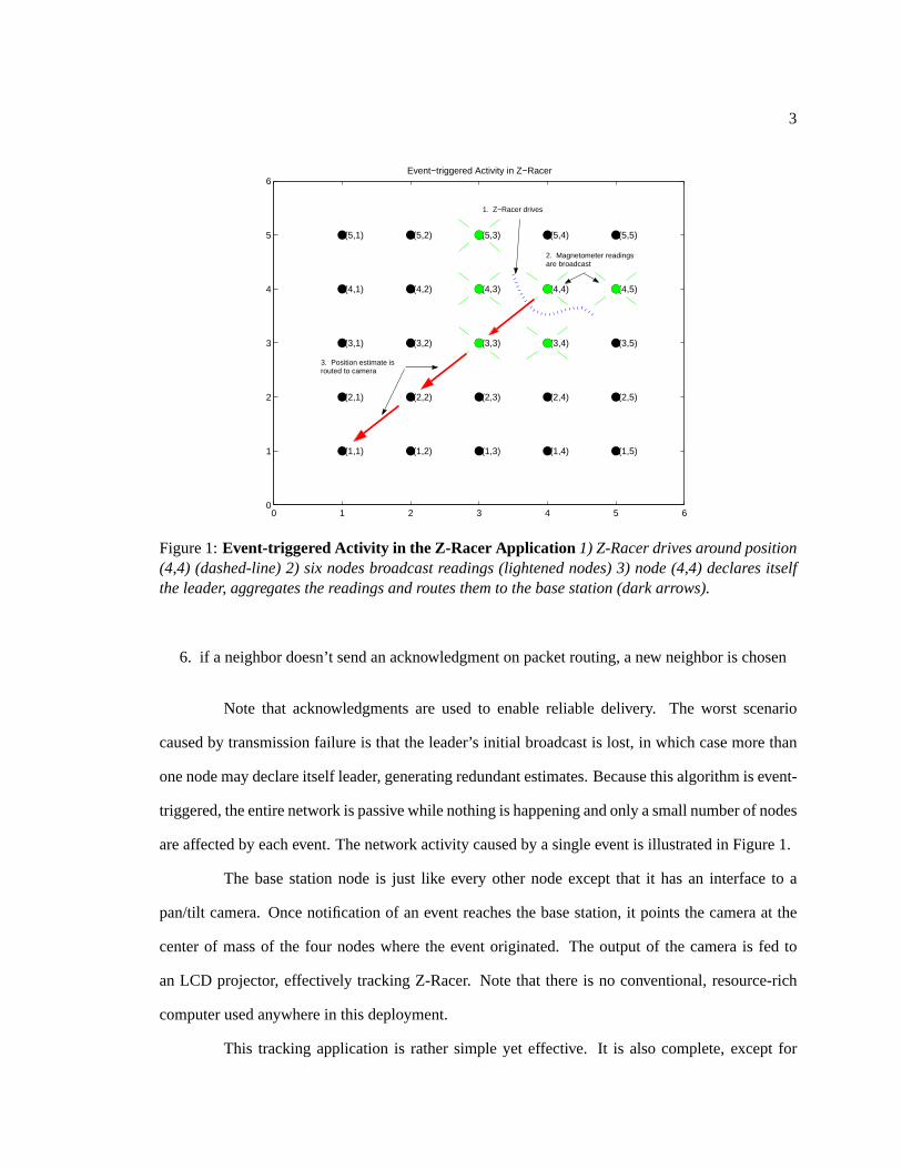
Figure 1:Event-triggered Activity in the Z-Racer Application 1) Z-Racer drives around position(4,4) (dashed-line) 2) six nodes broadcast readings (lightened nodes) 3) node (4,4) declares itselfthe leader, aggregates the readings and routes them to the base station (dark arrows).

6. if a neighbor doesn’t send an acknowledgment on packet routing, a new neighbor is chosen

Note that acknowledgments are used to enable reliable delivery. The worst scenario

caused by transmission failure is that the leader’s initial broadcast is lost, in which case more than

one node may declare itself leader, generating redundant estimates. Because this algorithm is event-

triggered, the entire network is passive while nothing is happening and only a small number of nodes

are affected by each event. The network activity caused by a single event is illustrated in Figure 1.

The base station node is just like every other node except that it has an interface to a

pan/tilt camera. Once notification of an event reaches the base station, it points the camera at the

center of mass of the four nodes where the event originated. The output of the camera is fed to

an LCD projector, effectively tracking Z-Racer. Note that there is no conventional, resource-rich

computer used anywhere in this deployment.

This tracking application is rather simple yet effective. It is also complete, except for

4

the glaring fact that each node must be pre-programmed with its own location. As in most sensor

network applications, however, location information is critical for the interpretation of sensor data.

The rest of this paper aims to provide this missing piece without compromising the simplicity of

this application or overburdening its resources.

3 Design Principles

In this section we derive four simple design principles from the Z-Racer application with

which to design a localization system.

3.1 Node-level Resolution

In the application above, the position of Z-Racer was determined up to node-level resolu-

tion. This will in fact be true for most sensor network applications since the nodes must be spaced

at less than twice the Nyquist interval of the spatial frequency of the phenomenon being observed.

For example, if one is measuring temperature fluctuations and nodes are spaced at one-meter inter-

vals, it is usually safe to assume that the user is interested in the position of a particular temperature

reading only up to one-meter resolution. If the nodes are spaced at two-inch intervals, however, one-

meter resolution is clearly not sufficient. This implies that the resolution of a localization system

for sensor networks must grow with the density of the network.

3.2 Scalable Deployment

Z-Racer is scalable in the sense that the computation, power, bandwidth, and infrastruc-

ture costs do not increase as the network grows. However, it is not entirely scalable in terms of

deployment because every node must be hand-placed and programmed with its location. Since

the size of a sensor network can be arbitrarily large, the infrastructure and deployment time of a

localization system for sensor networks should grow slower than the size of the network.

5

3.3 Event-driven

As previously noted, the Z-Racer application is completely event-driven, which is critical

for resource conservation. Similarly, since sensor nodes are often stationary, a localization system

should be active only in the rare event that nodes move or new nodes appear. In effect, the system

can be event-driven instead of ultra-low power. This philosophy of resource conservation is also

seen in [16], where ultra-low power sensor networks are those that sleep on the order of 97% of the

time.

3.4 Simple and Approximate Operation

The Z-Racer application was optimized for simplicity over accuracy and optimality, as

we can see in the multi-hop routing and Z-Racer positioning algorithms. An ultrasonic or laser

range finder could have been used to locate Z-Racer. However, cheap, simple and approximate

hardware is often as important in sensor networks as simple and approximate algorithms. Any

ad-hoc localization system for sensor networks cannot use high-power hardware or sophisticated

algorithms on the sensor nodes, no matter how accurate.

4 Existing Localization Systems

Localization is a very broadly-used capability that is required in several application do-

mains including ubiquitous computing, robotics, virtual reality and military planning. Each of these

applications has a different set of goals and constraints in terms of accuracy, infrastructure, de-

ployment time, instrumentation, power consumption, etc. For example, Microsoft’s RADAR [1] is

optimized for convenience while AT&T’s Active Bats [7] is optimized for high precision. Note that

neither system encompasses the other’s application domain and, furthermore, neither system could

use GPS [12], which is optimized for coarse-grained resolution outdoors. Unfortunately, localiza-

tion ishard in the sense that each application domain has typically required a new system to be built

6

from the ground up.

In this section we will explore four existing localization systems in terms of the goals

and constraints of sensor networks, as listed in the previous section. As we will see, very simple

differences in application constraints for each system have led to fundamentally different design

approaches. We will not review systems such as RADAR and Active Bats that are clearly not

designed for sensor networks; for a more complete survey see [8].

4.1 GPS

GPS was designed for global outdoor localization, which is useful for example in military

logistical operations. With this goal in mind, it was optimized for course-grained resolution, robust-

ness, and minimal user instrumentation. This was achieved through a multi-million dollar satellite

infrastructure that took years to build and deploy.

While one could argue that the power consumption of a GPS receiver is too high to run

on a sensor node, this is actually not a large concern for stationary nodes that only need to localize

infrequently. In fact, single-chip GPS solutions have been developed [30] and even integrated with

the Mica sensor platform. A more pressing concern is that even the best GPS receivers do not claim

more than 2-3 meter resolution and can see up to 10-20 meter error. GPS therefore does not meet

the node-level resolution requirements of sensor networks, severely limiting the spatial frequencies

that can be monitored with sensor networks.

4.2 Cricket

MIT’s Cricket was designed for the context-aware, ubiquitous computing environment.

Such applications need fine-grained three-dimensional location and orientation information, so

Cricket was optimized for centimeter-level resolution. This was achieved through the precise place-

ment of acoustic beacons on the ceiling and walls of each room.

The constraints of the ubiquitous computing environment, however, are very different

7

from those of sensor networks. One strict constraint in ubiquitous computing is that user location

information must be kept private. Cricket receivers thereforeself-localizeby passively listening

to beacons, which are constantly emitted from the infrastructure. Passive receivers mean that the

system is inherently not event-driven and, since each node must be in direct contact with at least

four beacons, deployment is not scalable in the sense that an ad-hoc system would be. Since sensor

networks have no privacy constraint, the infrastructural and power costs can be further optimized.

4.3 AHLoS

AHLoS, currently under development at UCLA, uses ultrasound technology similar to

cricket but does not contend with privacy constraints, allowing several developments in ad-hoc

localization. This system is ad-hoc in the sense that each node uses its neighbors to estimate its

own position. It is also fully distributed and functions both indoors and outdoors, satisfying many

requirements of most sensor network applications.

The technology is currently being deployed in a “Smart Kindergarten” setting where chil-

dren and toys can be tracked to high accuracy. In order to achieve the required spatial and temporal

resolution, the Medusa node used with AHLoS requires an Atmel ARM Thumb processor, four ul-

trasound transmitters and four receivers. A real-time tracking application, however, is very different

from a typical passive, long-duration stationary sensor network deployment. Sensor networks often

require only node-level resolution and sensor nodes are typically stationary or move infrequently.

We can leverage these properties, specific to sensor networks, to further optimize the hardware, al-

gorithmic complexity and computational costs while still satisfying the low-accuracy requirements

of sensor networks.

4.4 Millibots

An interesting approach to localization is found in the robotics literature. Millibots is

a project at CMU devoted to designing teams of miniature robots. Many system constraints such

8

as power, computation time and bandwidth are similar in these two problem domains. However,

because Millibots are mobile it is reasonable to assume they all robots are within radio range of

all other robots. They use a“leap-frog” approach to move as a group while ensuring that at least

three robots serve as stationary beacons for the rest of the robots. This assumption has allowed a

centralized approach to localization, where all computation is performed by a groupleader[14]. In

sensor networks, on the other hand, we are interested in large ad-hoc deployments over vast areas

where a centralized or leader approach would not be feasible.

5 Calamari Overview

In this section we presentCalamari, an ad-hoc localization system for sensor networks.

Calamari takes advantage of several unique properties of sensor networks that do not exist in the ap-

plication domains of the four systems mentioned above. These include stationarity of node configu-

ration, multiplicity of nodes, and node-level resolution requirements. These assumptions allow us to

optimize the localization system down to a level that is feasible in the highly power-, computation-

, and bandwidth-constrained environment of sensor networks. In the next three sections we will

discuss the design decisions of the main components of Calamari: the ranging technology, the cali-

bration procedure, and the localization algorithm. Here, we provide a brief overview.

The ranging technology is a combination of radio signal strength and acoustic time of

flight, both of which have different error distributions and failure modes. In order to minimize the

amount of hardware used, time of flight readings are taken using audible frequency range hardware

which is very low power and small enough to fit easily on a sensor node. Because the devices are not

optimized for ranging and because the frequency is ten times lower than the ultrasound hardware

typically used in ranging, we pay a factor of approximately ten in error. However, as we will see

this should still be sufficient to achieve the accuracy we need for sensor network applications.

While calibrating hardware can reduce ranging errors dramatically, calibrating each de-

vice can become tedious as networks grow to hundreds or thousands of nodes. Furthermore, unlike

9

systems like GPS or Cricket where each node can be calibrated against the infrastructure, each node

in an ad-hoc system like Calamari seemingly needs to be calibrated againsteveryother node. Such

pair-wise calibration takes timeO(n2) wheren is the number of nodes in the network. Calamari

uses a parameter estimation technique to solve both of these problems at once by calibrating the

network as a system instead of each node individually. Special ranging protocols are designed for

the distributed management of calibration parameters.

Once all nodes have distance estimates to their neighbors, they must use that information

to estimate their own locations. While single-node multilateration can be reduced to a simple set

of simultaneous linear equations, ad-hoc multilateration is a combinatorial problem to which there

is as of yet no optimal algorithm. Calamari uses a variant of APS [19], an ad-hoc analog to GPS,

which is a simple approximation to the true multilateration solution that scales well with network

size. We analyze APS in terms of our known ranging error distributions and suggest modifications

that reduce error by 20-30%.

The following sections outline the design decisions made for each of the three components

of Calamari and present the data and arguments that motivated each decision.

6 The Ranging Technology

The ranging technology is the heart of any localization system; its error characteristics

and failure modes often determine the design and applicability of the rest of the system. This

section evaluates three different ranging technologies that can be used with Calamari: connectivity

or hop-based measures, radio signal strength, and acoustic time of flight.

There are several features that make these three ranging technologies well-suited to sensor

network localization. They can all give long-range estimates in roughly all directions, unlike some

methods, such as infrared [31], which are directional. Furthermore, they all use small, cheap and

low-power hardware that can be used by every single node. This allows a peer-to-peer localization

strategy that cannot be had with technologies such as laser ranging or magnetic ranging [23]. Finally,

10

each of these techniques is extremely simple and does not overburden a sensor node or the network.

In this section, each method is analyzed in terms of cost, range, error characteristics and

failure modes. Notice that the error rates that we see in this section are for a known transmitter and

receiver. The task of calibrating devices to ensure that all transmitters and receivers behave alike is

left until section 7

6.1 Radio Connectivity and Hop-based Measures

Many algorithms and theoretical results in ad-hoc networking and localization are based

on a disc approximation to radio connectivity [17]. For example, work by [6] proved the existence

of a phase transition in network connectivity when each node has an average of4.5 neighbors. Work

by [3] has shown that the disc approximation allows one to frame ad-hoc localization as a convex

optimization problem. Other work in distributed localization algorithms [19, 25] implicitly use radio

connectivity by estimating distances with hop counts. If radio connectivity were a good indicator

of distance, it would be the cheapest and easiest ranging technique since it could just piggy-back on

the network routing protocols.

There are many reasons, however, why a disc may be a bad approximation to radio con-

nectivity. Asymmetries in the environment or in the antenna’s orientation or propagation model

greatly affect radio connectivity. The world is rarely symmetrical and even small environmental

factors can cause large deviation from a disc model.

One further problem with the disc approximation is that it requires a sharp division be-

tween pairs of nodes that areconnectedand those that are not. However, a rather large portion of

the radio range actually exhibits a stochastic behavior where the radios are neither connected nor

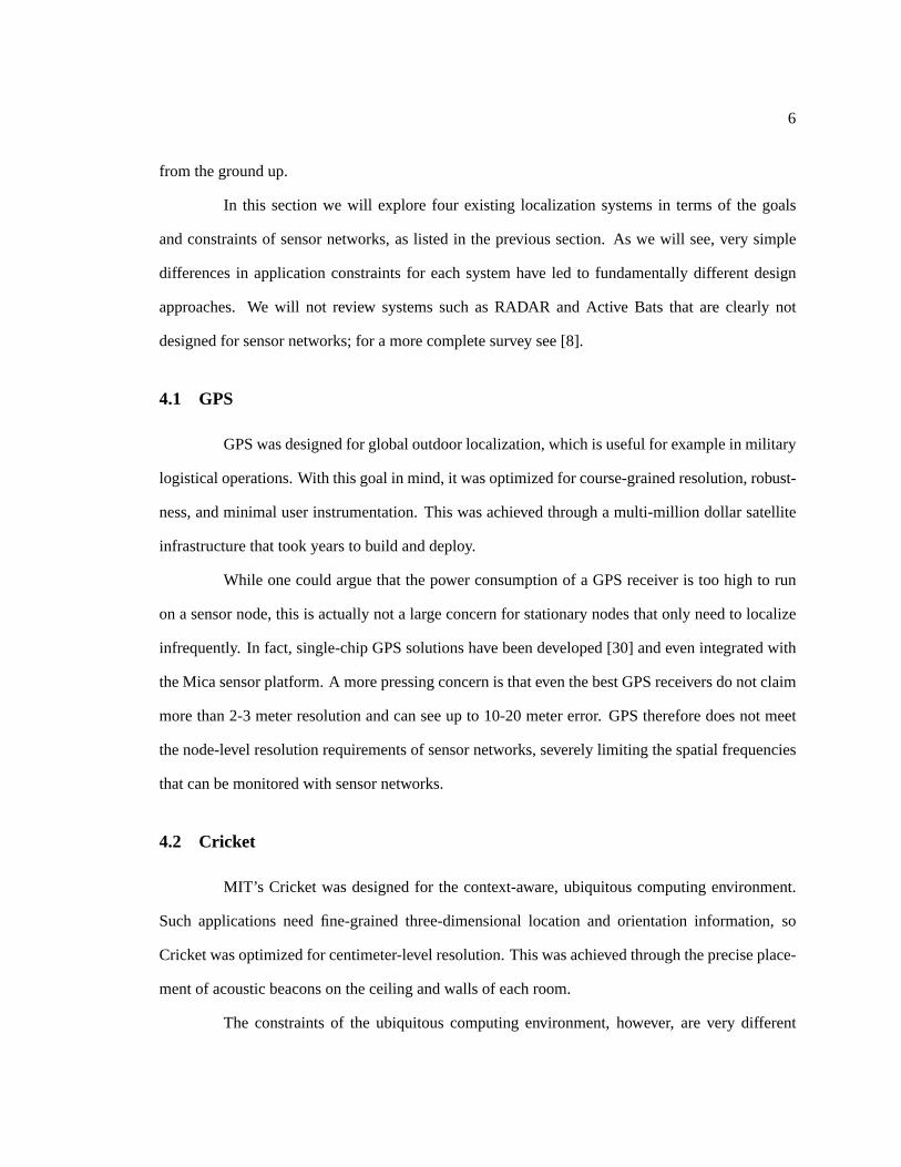
disconnected but rather have some probability of being connected. This is seen in Figure 2, which

depicts the probability of successful transmission between each pair of nodes as a blue dot plotted

as a function of the distance between them. This data indicates three problems for a disc model of

2Figures 2, 3, and 4 courtesy of Alec Woo. Much data from Section 6.1 is from [4].

11

Figure 2:Radio Connectivity over Distance2is stochastic for a large portion of the radio range.Each circle represents the probability of successful transmission plotted as a function of distancefor each of 147 transmitter/receiver pairs.

connectivity. First, it is unclear how to defineconnectivity. Second, no definition of radio connec-

tivity will correctly separate pairs of nodes into those that are farther and those that are closer than

a given distance. Third, many pairs whose connectivity falls near the boundary of connectivity will

tend to oscillate between being closer to and farther than that distance.

Even if eachpair of transceivers did have disc-like connectivity, however, the size of this

disc may be different for each pair due to variations in the transceivers themselves. Therefore, even

in an ideal environment the connectivity model betweenall transceivers may not be well approxi-

mated by a disc. This can be seen in Figure 3 which shows the probability of packet reception for

147 Rene motes laid out in a 2-foot grid on a tennis court. The Rene motes are using monopole

antennas in an upright position and the RFM TR1000 radio transceiver [24]. For this particular

node, the farthest node that can hear it is more than 400% farther than the closest node that cannot.

It is unclear how non-disc-like connectivity affects hop count. In the best case connectivity

variations are unbiased, allowing errors to cancel out over long distances. At the least, stochastic

12

1 2 3 4 5 6 7 8 9 10 11 12

2

4

6

8

10

12

14

Grid Column

Probability of Packet Transmission: Transmitter #254

Grid

Row

0

0.2

0.4

0.6

0.8

1

Figure 3:Connectivity over Spaceis not necessarily disc-like, as seen in this figure where proba-bility of successful transmission is indicated by color. A single transmitter is located at(6,6) in a 12x 14 grid of 147 nodes. All nodes are identically oriented on a tennis court with 2-foot spacing.

Figure 4:Trace of Network Flood from a147 node experiment reveals unpredictable propagationpatterns due to collisions and irregular connectivity. Node45 is eleven times as far from(0,0) asnode184, but both are two hops away.

13

connectivity becomes a logistical problem when measuring hop counts. Figure 4 shows the message

propagation through a network of 147 nodes in an 12 x 13 grid. In this case, hop count is clearly

an extremely unreliable indicator of distance after a single flood of the network. Furthermore, it is

unclear that subsequent floods will not be subject to the same systematic failures that occurred in

the first flood. This argues that radio connectivity must be performed with neighborhood monitoring

instead of controlled network flooding, as proposed in [19, 25].

6.2 Radio Signal Strength

Several localization systems have used received radio signal strength to estimate distance

between transmitter and receiver. Perhaps the most well known of these is RADAR [1] which uses

existing 802.11 networks. Other commercial systems include PinPoint [21] and WhereNet [32]

which deploy specialized RF infrastructure. Recent research in ad-hoc localization using signal

strength include SpotON [9] and AHLoS [26]. The current default radio protocol used with TinyOS

[10] measures signal strength with each radio message sent. This section analyzes exactly how

useful this information might be in localization.

It is well known that signal strength information is an unreliable indicator of distance in

complex indoor or urban environments due to obstacles and reflections. This is especially problem-

atic because erroneous readings give no indication of being erroneous, causing heavy-tailed error

distributions which are difficult to deal with. This does not, however, mean that signal strength is

not applicable in sensor networks. Indeed, many sensor network applicationsare situated in ideal

settings for measuring signal strength, e.g. outdoors. Furthermore, in less than ideal environments,

signal strength can be used to corroborate measurements from other ranging technologies which

might have different failure modes. Such multi-modal fusion for localization is being explored in

several different literatures.

Assuming an isotropic transmitting antenna and a near-ideal environment, signal strength

at a receiver with distancer from a transmitter is proportional toRArwhereR is the surface area of

14

−5 0 5 10 15 20 25 30 35 40 451.3

1.35

1.4

1.45

1.5

1.55

1.6

1.65

1.7

1.75Average Signal Strength over Distance

Distance (ft)

Sig

nal S

tren

gth

(V)

Figure 5:Average Signal Strength Readingsdecay logarithmically over distance in a near-idealenvironment.

the receiver andAr is the surface area of a sphere with radiusr. SinceR is constant and the area

of a sphere is proportional to1r2 , this ratio will shrink by a factor of14 asr doubles. In other words,

received signal strength will decrease by10 log10(4) = 6dB asr doubles.

Signal strength readings on motes are taken by sending an extended RF pulse using the

RFM TR1000 radio to send a clean 916.5MHz signal. The receiver samples theBBOUT pin on

the RFM, which varies at about 10mV/dB [24]. Figure 5 shows the observed mean and standard

deviation of signal strength as distance increases. As the theory above dictates, this curve decreases

logarithmically. What we are interested in is theranging error that would be achieved at each

distance using this curve. This is determined by both the noise in the signal strength readings and

the signal strength attenuation rate, i.e. the slope of the line above. Assuming slope is roughly

constant over short distances, we can approximate this with

error (cm)≈ noise (dB)

attenuation rate(dBcm)

(0.1)

15

−5 0 5 10 15 20 25 30 35 40 451.3

1.35

1.4

1.45

1.5

1.55

1.6

1.65

1.7

1.75Average Signal Strength over Distance

Distance (ft)

Sig

nal S

tren

gth

(V)

SmallError

LargeError

Figure 6:Error Increase over Distancedepends on bothnoiseandattenuation rate. As the atten-uation rate flattens out, differences in signal strength become small relative to noise levels.

0 5 10 15 20 25 30 350

20

40

60

80

100

120Noise(V) / Rate of Attenuation (V/ft)

Distance (ft)

Err

or

Figure 7:Signal Strength Ranging Error increases with distance due to the increase in noise andthe logarithmic decrease in signal strength. The values in this graph are calculated directly fromthe data in Figure 5 and from eq ( 0.1)

16

−0.04 −0.03 −0.02 −0.01 0 0.01 0.02 0.030

2

4

6

8

10

12Distribution of Noise in Signal Strength

Noise (V)

Num

ber

of O

ccur

ence

s

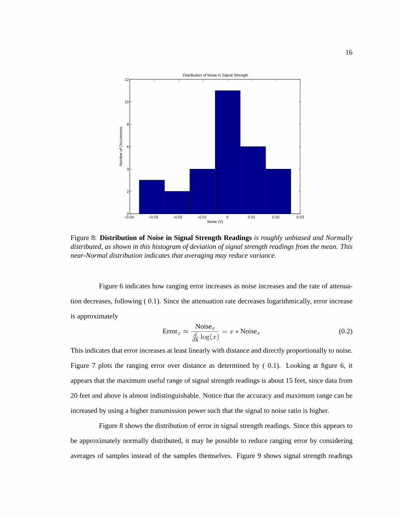
Figure 8:Distribution of Noise in Signal Strength Readingsis roughly unbiased and Normallydistributed, as shown in this histogram of deviation of signal strength readings from the mean. Thisnear-Normal distribution indicates that averaging may reduce variance.

Figure 6 indicates how ranging error increases as noise increases and the rate of attenua-

tion decreases, following ( 0.1). Since the attenuation rate decreases logarithmically, error increase

is approximately

Errorx ≈ Noisexd

dx log(x)= x ∗ Noisex (0.2)

This indicates that error increases at least linearly with distance and directly proportionally to noise.

Figure 7 plots the ranging error over distance as determined by ( 0.1). Looking at figure 6, it

appears that the maximum useful range of signal strength readings is about 15 feet, since data from

20 feet and above is almost indistinguishable. Notice that the accuracy and maximum range can be

increased by using a higher transmission power such that the signal to noise ratio is higher.

Figure 8 shows the distribution of error in signal strength readings. Since this appears to

be approximately normally distributed, it may be possible to reduce ranging error by considering

averages of samples instead of the samples themselves. Figure 9 shows signal strength readings

17

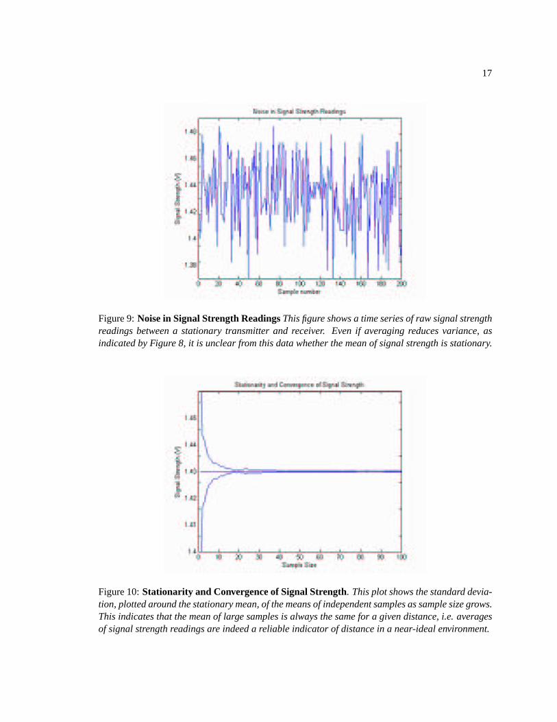
Figure 9:Noise in Signal Strength ReadingsThis figure shows a time series of raw signal strengthreadings between a stationary transmitter and receiver. Even if averaging reduces variance, asindicated by Figure 8, it is unclear from this data whether the mean of signal strength is stationary.

Figure 10:Stationarity and Convergence of Signal Strength. This plot shows the standard devia-tion, plotted around the stationary mean, of the means of independent samples as sample size grows.This indicates that the mean of large samples is always the same for a given distance, i.e. averagesof signal strength readings are indeed a reliable indicator of distance in a near-ideal environment.

18

Figure 11:Noise due to Reflections and Obstructionswill systematically affect signal strengthreadings, indicating that signal strength is not useful in non-ideal environments even afteraveraging.

over time at a constant distance. We want to analyze the stationarity and convergence rate of the

noise in this data, i.e. determine the standard deviationσ of averages ofn data points and observe

thatσ → 0 asn → ∞. Figure 10 shows the variance of sample averages as sample size increases.

Since the noise is normally distributed, the means converge exponentially quickly as sample size

grows. This data is clearly stationary sinceσ → 0, indicating that error can be reduced by using

averages.

While this method of noise reduction seems promising, it does not mean that any distance

can be estimated with arbitrary accuracy given an infinite number of samples. This is because of

systematic error caused by the environment, such as reflections or obstructions, which increases

as distance grows. Figure 11 shows the distance estimates and their correspondingσ values using

averages of signal strength readings over a short distance. At such small values ofσ the systematic

error caused by the environment becomes very apparent from the bumpiness of the curve. As

mentioned before, this phenomenon is even more problematic than if we were not able to reduce

19

the error estimates; we have no way of knowing if an estimate is erroneous or not.

The most severe problem with this ranging modality will be addressed in Section 7 of this

paper. It turns out that the variations between radio transceivers have an effect on signal strength

that is comparable to the effect of distance. Indeed, this is exactly the problem we saw with radio

connectivity and hop-based metrics. However, while calibration coefficients for each node would

not help a connectivity metric, they will help us to correctly interpret signal strength readings.

Tracking

The speed with which one can achieve a given error rate is determined by the number

of samples required to achieve the corresponding noise level. This calculation is important for

tracking. For example, suppose we wanted to track a moving object with1cm resolution and we

need40 samples to achieve1cm error. Assuming we can sample at1000Hz, we need at least40msec

to collect the required samples. Naturally, we need to do this before the object can move more than

1cm, so it can move at most1cm40msec ≈ .9Km

hr , which is to say that radio signal strength cannot be

used to track quickly moving objects very accurately. While this technology may therefore not be

effective in some problem domains such as tracking, it is appropriate for sensor network applications

in which nodes are typically stationary.

6.3 Acoustic Time of Flight

Acoustic time of flight is a popular ranging technology with existing localization sys-

tems. Among these systems are AT&T’s Active Bats [7], MIT’s Cricket [22], UCLA’s AHLoS [26]

and many robotic systems, including CMU’s Millibots [14]. All of these systems use ultrasound

transceivers, which are small, low-power, cheap and highly accurate. This section discusses both

ultrasound and audible-frequency ranging techniques.

Acoustic time of flight is measured in Calamari by simultaneously sending a radio mes-

sage with an acoustic pulse. All radio messages in TinyOS are already time stamped with micro-

20

0 20 40 60 80 100 120 140 160 1800

20

40

60

80

100

120

140

160Ultrasound Distance Estimates vs Distance

Distance (cm)

Dis

tanc

e E

stim

ate

(cm

)

Figure 12:Average Distance Estimate with Ultrasound Ranging4are quite accurate and growlinearly with distance

second accuracy. When an acoustic pulse is received, it signals an interrupt on the processor that is

also time stamped with micro-second accuracy. The only computational cost in obtaining a distance

estimate is to subtract these time stamps and multiply the difference by the speed of sound. We will

analyze the error of the distance estimates that emerge using two different acoustic ranges.

Ultrasound

The above technique was used with an ultrasound board designed for AHLoS [26] and

used on the Mica mote. The board uses the Kobitone ultrasound transmitter/receiver pair [18]. The

average value of 100 samples at each distance is shown in Figure 12 and the corresponding error

rates according to equation ( 0.1) are shown in Figure 13. Since the error rates are lower than the size

of the Mica node itself, this ranging technique is clearly capable of achieving node-level resolution

with Calamari.4Data shown in Figure 12 was collected by Fred Jiang using ultrasound boards courtesy of Andreas Savvides [27].

21

20 30 40 50 60 70 80 90 100 110 1200

1

2

3

4

5

6Ultrasound Noise(cm) / Rate of Attenuation (cm/cm)

Distance (cm)

Err

or (

cm)

Figure 13:Ranging Error with Ultrasound Ranging is seen to be less than 5cm for distances upto 120cm.

One problem, however, is that these transmitter/receivers are highly directional; the de-

vices have a120o cone of transmission, outside of which they cannot obtain a ranging estimate at

all. Furthermore, ranging estimates degrade as the central axes of the transmitter and receiver devi-

ate from each other. Unlike systems like Cricket [22] that can assume transmitters are on the ceiling

or walls, sensor nodes in our application may encounter other sensor nodes anywhere around them.

Furthermore, since the node will not in general know its own orientation, it must be able to range in

multiple directions in order to find its position.

One solution to this problem is to use many transmitter/receiver pairs. Indeed, another

board is being designed for AHLoS which has four such pairs; it is able to estimate distance in

almost any direction. This solution, however, essentially doubles the size of a sensor node; eight ul-

trasound casings are large enough to cover almost the entire surface area of the Mica mote, leaving

little room for actual sensors. The Dot mote is barely large enough to even carry one transmit-

ter/receiver pair. While ultrasound is a viable ranging technology for sensor networks when high

22

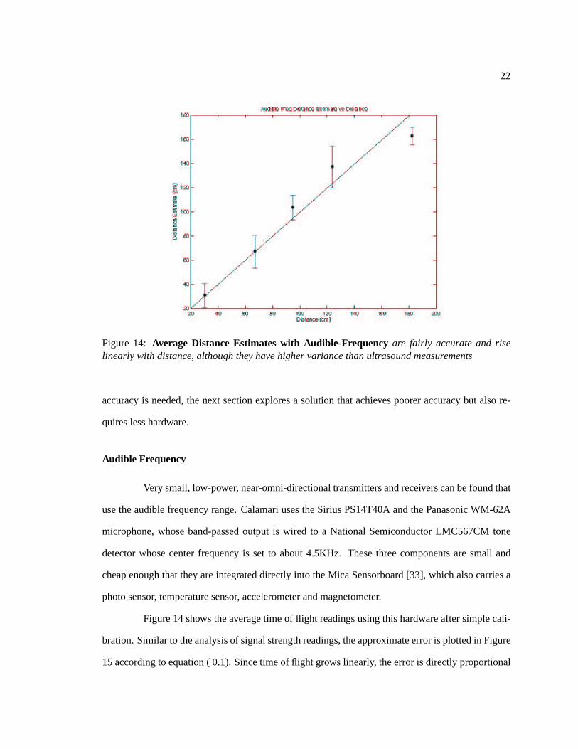
Figure 14: Average Distance Estimates with Audible-Frequencyare fairly accurate and riselinearly with distance, although they have higher variance than ultrasound measurements

accuracy is needed, the next section explores a solution that achieves poorer accuracy but also re-

quires less hardware.

Audible Frequency

Very small, low-power, near-omni-directional transmitters and receivers can be found that

use the audible frequency range. Calamari uses the Sirius PS14T40A and the Panasonic WM-62A

microphone, whose band-passed output is wired to a National Semiconductor LMC567CM tone

detector whose center frequency is set to about 4.5KHz. These three components are small and

cheap enough that they are integrated directly into the Mica Sensorboard [33], which also carries a

photo sensor, temperature sensor, accelerometer and magnetometer.

Figure 14 shows the average time of flight readings using this hardware after simple cali-

bration. Similar to the analysis of signal strength readings, the approximate error is plotted in Figure

15 according to equation ( 0.1). Since time of flight grows linearly, the error is directly proportional

23

30 40 50 60 70 80 90 100 110 120 13013

14

15

16

17

18

19

20

21

22

23Audible Freq Noise(cm) / Rate of Attenuation (cm/cm)

Distance (cm)

Err

or (

cm)

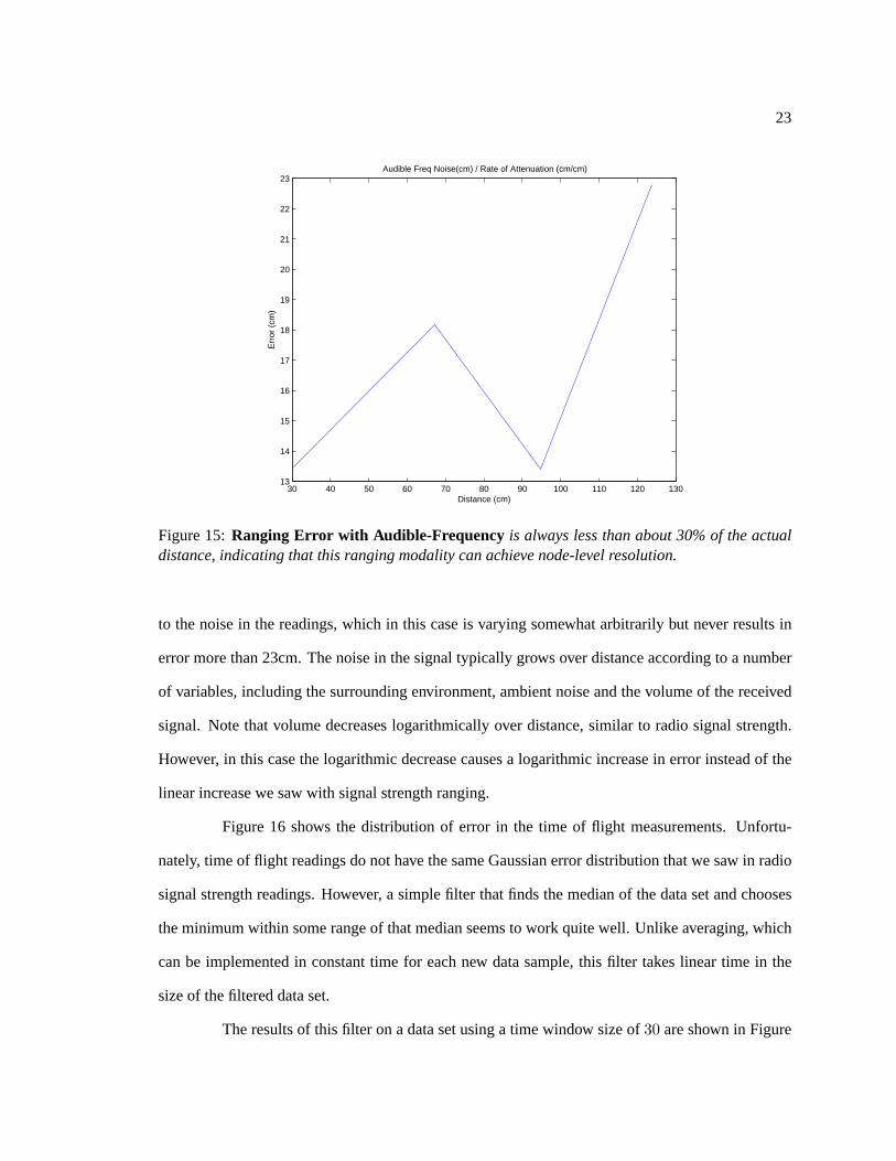
Figure 15:Ranging Error with Audible-Frequency is always less than about 30% of the actualdistance, indicating that this ranging modality can achieve node-level resolution.

to the noise in the readings, which in this case is varying somewhat arbitrarily but never results in

error more than 23cm. The noise in the signal typically grows over distance according to a number

of variables, including the surrounding environment, ambient noise and the volume of the received

signal. Note that volume decreases logarithmically over distance, similar to radio signal strength.

However, in this case the logarithmic decrease causes a logarithmic increase in error instead of the

linear increase we saw with signal strength ranging.

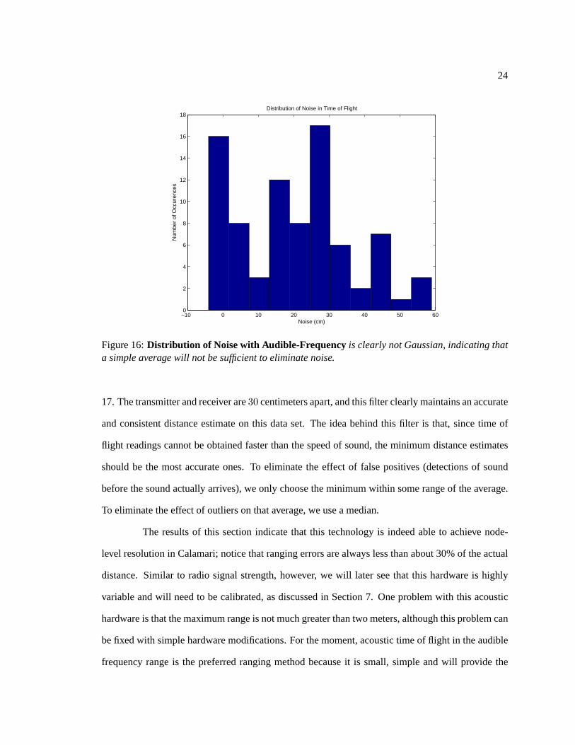
Figure 16 shows the distribution of error in the time of flight measurements. Unfortu-

nately, time of flight readings do not have the same Gaussian error distribution that we saw in radio

signal strength readings. However, a simple filter that finds the median of the data set and chooses

the minimum within some range of that median seems to work quite well. Unlike averaging, which

can be implemented in constant time for each new data sample, this filter takes linear time in the

size of the filtered data set.

The results of this filter on a data set using a time window size of30 are shown in Figure

24

−10 0 10 20 30 40 50 600

2

4

6

8

10

12

14

16

18Distribution of Noise in Time of Flight

Noise (cm)

Num

ber

of O

ccur

ence

s

Figure 16:Distribution of Noise with Audible-Frequency is clearly not Gaussian, indicating thata simple average will not be sufficient to eliminate noise.

17. The transmitter and receiver are30 centimeters apart, and this filter clearly maintains an accurate

and consistent distance estimate on this data set. The idea behind this filter is that, since time of

flight readings cannot be obtained faster than the speed of sound, the minimum distance estimates

should be the most accurate ones. To eliminate the effect of false positives (detections of sound

before the sound actually arrives), we only choose the minimum within some range of the average.

To eliminate the effect of outliers on that average, we use a median.

The results of this section indicate that this technology is indeed able to achieve node-

level resolution in Calamari; notice that ranging errors are always less than about 30% of the actual

distance. Similar to radio signal strength, however, we will later see that this hardware is highly

variable and will need to be calibrated, as discussed in Section 7. One problem with this acoustic

hardware is that the maximum range is not much greater than two meters, although this problem can

be fixed with simple hardware modifications. For the moment, acoustic time of flight in the audible

frequency range is the preferred ranging method because it is small, simple and will provide the

25

0 20 40 60 80 100 120 140 160 180 2000

15

30

45

60

75

90

105Filtered Time of Flight Estimates

Time (sec)

Dis

tanc

e E

stim

ate

(cm

)

Raw Distance EstimatesFiltered Distance Estimates

False positives

Outliers

Normal Noise

Figure 17:Filtering Time of Flight Estimates is done by taking the minimum within some rangeof the median. This reduces the effect of normal noise, outliers, and false positives. The filteredestimate matches the true estimate of30 centimeters while the unfiltered estimate varies greatly.

26

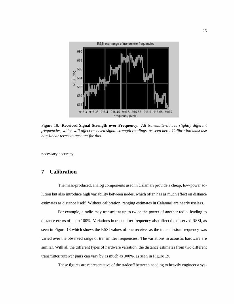
Figure 18: Received Signal Strength over Frequency. All transmitters have slightly differentfrequencies, which will affect received signal strength readings, as seen here. Calibration must usenon-linear terms to account for this.

necessary accuracy.

7 Calibration

The mass-produced, analog components used in Calamari provide a cheap, low-power so-

lution but also introduce high variability between nodes, which often has as much effect on distance

estimates as distance itself. Without calibration, ranging estimates in Calamari are nearly useless.

For example, a radio may transmit at up to twice the power of another radio, leading to

distance errors of up to 100%. Variations in transmitter frequency also affect the observed RSSI, as

seen in Figure 18 which shows the RSSI values of one receiver as the transmission frequency was

varied over the observed range of transmitter frequencies. The variations in acoustic hardware are

similar. With all the different types of hardware variation, the distance estimates from two different

transmitter/receiver pairs can vary by as much as 300%, as seen in Figure 19.

These figures are representative of the tradeoff between needing to heavily engineer a sys-

27

0 50 100 150 200 2500

50

100

150

200

250

300

350

400

450

500

True Distance (cm)

Est

imat

ed D

ista

nce

(cm

)

Uncalibrated Distance Estimates

Figure 19:Uncalibrated TOF readings are always greater than the true distance and are highlyerroneous due to transmit- and receive-delays.

tem and needing to heavily calibrate it. The rest of this paper shows how we solve these calibration

problems instead of adding extra specialized hardware, using expensive digital signal processing, or

adding infrastructure. Unfortunately, as we see in the next section, traditional calibration is not an

adequate solution and we need to find more powerful techniques.

7.1 Traditional Calibration

Device calibration is the process of forcing a device to conform to a given input/output

mapping. This is often done by adjusting the device internally but can equivalently be done by

passing the device’s output through acalibration functionthat maps the actual device response to

the desired response. In this paper, we will focus on the latter method because it is easily compared

to the methods used in macro-calibration.

A more formal description of calibration is this: each device has a set of parameters

β ∈ <p. The purpose of calibration is to choose the correct parameters for each device such that

28

they, in conjunction with a calibration function, will translate any actual device outputr into the

corresponding desired outputr∗. The calibration function must therefore be of the form

r∗ = f(r, β) (0.3)

In traditional calibration, we observe the device in a controlled environment and map its

observed outputr to the desired outputr∗, perhaps using a form of regression or even simply a

lookup table.

To see why traditional calibration is inadequate for Calamari, let us try to use it to calibrate

our ranging system. Assume we have a transmitter and receiver that give distance estimatesd1, d2,

andd3 at known distancesd∗1, d∗2, d∗3. According to the traditional calibration framework, we need

to generate a function with parametersβ that map the estimates to the true distances. Let us try

doing this with linear regression. First, we assume thatr∗ is a linear function ofr, giving us the

following calibration function:

r∗ = β1 + β2 · r (0.4)

Plugging in our three distance estimates and their known distances, we get a system of

equations which we can easily solve for our parametersβ1 andβ2:

d∗1 = β1 + β2 · d1 (0.5)

d∗2 = β1 + β2 · d2 (0.6)

d∗3 = β1 + β2 · d3 (0.7)

These parameters, along with our linear calibration function, can then be used with any future

distance estimatedt to estimate the true distanced∗t .

While traditional calibration does successfully give us a mapping from our actual response

to our desired response, neither parameter belongs to either the transmitter or the receiver, but rather

29

both belong to thetransmitter/receiver pair. We will call this pairwise calibrationsince we must

repeat this process for every such pair. This is clearly undesirable because the cost of pairwise

calibration is ordern2 wheren is the number of nodes in the system. Furthermore, we must manage

n2 sets of parameters.

We would prefer to calibrate each transmitter and each receiver individually as we would

for, say, a thermometer or magnetometer. That is, we would like to use an ordern calibration

method. The problem is that, under the traditional calibration framework just described, we need to

know both the device responser and the desired responser∗. However, the values ofr andr∗ in

ranging are inherently tied to both the transmitter and receiver.

In Calamari, as we can see, traditional calibration can do pairwise calibration but cannot

calibrate individual transmitters or receivers; there is only one response from the system and it

cannot separate the effect of the transmitter from the effect of the receiver. We will call this the

separation problem. In the following sections, we discuss three methods to overcome the separation

problem: iterative, mean, and joint calibration.

Towards Avoiding the Separation Problem

The separation problem is not specific to Calamari, but to the calibration of all sen-

sor/actuator pairs. We realize the importance of it when we see thatall calibration is between

sensor/actuator pairs. We usually do not worry about it when calibrating temperature sensors with

room temperature, but we might need to when calibrating, for example, magnetometers with a set

of magnets.

Iterative Calibration

The first attempt we see to circumvent the separation problem comes from the ad-hoc lo-

calization literature. SpotON [9] uses low-power radio transceivers in an RSSI ranging system very

similar to the RSSI component of Calamari. To calibrate, SpotON observes that the separation prob-

30

lem could be avoided if we had at least one calibrated transmitter or receiver. As a solution, it simply

declaresone transmitterTr to be the reference transmitter and uses it to calibrate all receivers. It

then uses one reference receiverRr to be the reference receiver and calibrate all transmitters.

This procedure effectivelyiteratestraditional calibration, so we will call ititerative cali-

bration. In both iterations there is only one uncalibrated device in each pair. When a measurement

from the pair is in error, the error is attributed to the uncalibrated device, thereby getting past the

separation problem.

More precisely, letdi be the distance between receiverRi and the reference transmitter

and letβi be that receiver’s calibration parameters. For each such receiver, we have a system of

equations of the form

d∗i = f(di, βi) (0.8)

which we can solve forβi. We now choose a reference receiverRr and the distance from it to each

transmitterTj is dj . For each such transmitter, we have a system of equations of the form

d∗j = f(dj , βj , βr) (0.9)

which we can solve forβj , whereβr is the set of parameters for the reference receiver that was

learned in the first iteration. Note that the parameters of each receiver are derived only from the

distance estimates between it and the reference transmitter, and vice versa for each transmitter.

An interesting part of the SpotON technique is that the receivers are not actually adjusted

at all. Instead, each receiver is parameterized in terms of the Seidel and Rappaport RF path loss

model. There are two main advantages to using this parameterization. First, the receiver sensitivity

cannot be adjusted in hardware anyway. Second, and more importantly, the parameterization can

be arbitrarily accurate. In fact, Hightower, et al take advantage of Gaussian noise in their data by

effectively using least-squares log-linear regression over 100 readings. This technique is expanded

upon in the present work.

There is one serious problem with iterative calibration as applied to SpotON. RSSI is

effected by thedifferencein frequency of the transmitter and receiver, as seen in Figure 18. The

31

farther the transmission frequency is from the center frequency of the receiver, the more the incom-

ing signal will be attenuated by the receiver. This means that a receiver’s calibration parameters are

only valid for a single frequency: that of the transmitter used to calibrate it. Iterative calibration

does not actually avoid the separation problem at all; calibration parameters are only known to be

valid for one transmitter/receiver pair.

Mean Calibration

Let us propose one-more attempt to avoid the separation problem. Here, we assume that

variations in the devices are Gaussian distributed. By doing so, we can calibrate all receivers to the

meanof the transmitters, or vice versa. Let us call this methodmean calibration. In mean calibration

one collects calibration data for each receiver usingall transmitters as calibrating devices. The

parameters learned for the receiver will not be coupled to any particular transmitter and will also

minimize the expected error for that receiver in the least-squares sense, assuming that the sample of

transmitters used represents the true transmitter population.

More precisely, letdi,j be the distance between receiverRi and transmitterTj . For each

receiver, we have a system of equations of the form

d∗i,j = f(di,j , βi) (0.10)

which we can solve forβi. Notice that, unlike iterative calibration, the parametersβi are not related

to any particular transmitter. If we use least squares techniques to solve the system of equations, we

are in fact calibrating each receiver to the mean of all transmitters.

Mean calibration trivially avoids the separation problem by not calibrating the transmitters

at all. While this system minimizes expected error for the receiver, however, it is unlikely that it

minimizes error for the system as a whole since the transmitters have not been calibrated. In the

next section, we describe a method that directly minimizes the error of the entire system.

32

7.2 Calibration in Calamari

Both methods that we have seen so far are micro-calibration processes. They directly ob-

serve each device and build a mapping fromr to r∗ to directly optimize that device’s response. In

this section, we will describe a method of macro-calibration that calibrates each device by optimiz-

ing the overall system response instead of the individual device responses.

The method has three steps:

1. Parameterize each individual device and model the system response as a whole using these

parameters

2. Collect data from the system as a whole

3. Choose the parameters for the individual devices such that the behavior of the entire system

is optimized

How does this technique choose parameters for individual devices while only observing

the system response? By observingtrendsin the transmitter/receiver pairs, we can attribute errors

in the system to the individual nodes that are likely to cause them. In other words, if all distance

estimates made with a particular transmitter are slightly high, we can blame that transmitter. By

looking at the entire system response at once, we can allocate blame optimally amongst the nodes.

The Parameterization

We choose parameters for the devices based on our physical understanding of their in-

teractions. We focus here on TOF ranging, although the parameterization is nearly identical for

RSSI.

In Calamari, an acoustic pulse of roughly 15ms is transmitted along with a 25ms radio

packet. When the microphone receives the acoustic pulse, the phase lock loop (PLL) of the tone

detector attempts to identify the signal. When the PLL response and the microphone response are

high enough in combination, an interrupt is fired which is time-stamped by the processor. This time

33

stamp is compared with the time stamp of the radio packet. The difference in time is multiplied by

the nominal speed of sound to obtain a distance estimate.

Several variations in the hardware strongly effect the TOF readings:

Bias – The times for the sounder and microphone to start oscillating,BT andBR, may vary

due to variations in the diaphragms

Gain – The volume of the sounder and the sensitivity of the microphone,GT andGR, affect

the speed with which the PLL detects the signal

Frequency– The difference in sounder frequency and tone detector center frequency,|FT −FR|, has a near-linear affect on the effective received volume.

Orientation – The relative orientations of the sounder and microphone,OT andOR, will

affect the volume with which the acoustic tone is received through some non-linear function

fO(·).

We therefore arrive at the following complete model of the system response for a trans-

mitter/receiver pair:

d∗ = BT + BR + GT · d + GR · d

+|FT − FR| · d + fO(OT , OR) · d (0.11)

Whered is the distance estimate andd∗ is the true distance between the pair.

Choosing the Parameters

Assuming we have collected data from our system, we may choose values for the device

parameters such that our sensor model above matches the data we collected. To simplify the process,

we will remove the non-linear parameters for frequency and orientation and allow both of these

factors to be built into the error term. Our simplified but less accurate sensor model becomes:

r∗ = BT + BR + GT · r + GR · r (0.12)

34

Each pair of collected valuesr andr∗ together with this model form an equation with four

variables. We collect one sample from each pair in our network, giving us4n variables inn2 − n

equations, wheren is the number of nodes. This system of equations will generally over-constrain

the values of all device parameters.

More precisely, letdi,j be the distance between receiverRi and transmitterTj . For each

transmitter and receiver, we have a system of equations of the form

d∗i,j = f(di,j , βi, βj) (0.13)

We cannot solve these equations for eitherβi or βj because there is no unique solution; there is

no way to know if error should be attributed to the transmitter or receiver parameters. However,

we can use all pairs of nodes to create a system ofn2 − n equations, which we can solve for all

4n parameters. Notice that, unlike iterative calibration and mean calibration, we do not calibrate

each device by solving a system of equations for that device. Instead, we calibrate the entire system

at once by solving a system of equations that relates that system. No parameter of a receiver or

transmitter is tied to any device other than that particular receiver or transmitter.

We can use least-squares [2] [20] to solve this system of equations by converting it into

matrix notation

Ax = b (0.14)

Let x be an array of our device parameters and let each row ofA be the coefficients from

our model of one data sampleb. For example, if our first two distance estimates wered1,2 andd1,3

coming from transmitter/receiver pairs(1, 2) and(1, 3), the first two rows of theA andb matrices

would be as follows:

A =

1 0 · · · 0 1 0 · · · d1,2 0 · · · 0 d1,2 0 · · ·1 0 · · · 0 0 1 · · · d1,3 0 · · · 0 0 d1,3 · · ·...

......

......

...

and

35

b =

d∗1,2

d∗1,3

...

where

x =

BT1

...

BTn

BR1

...

BRn

GT1

...

GTn

GR1

...

GRn

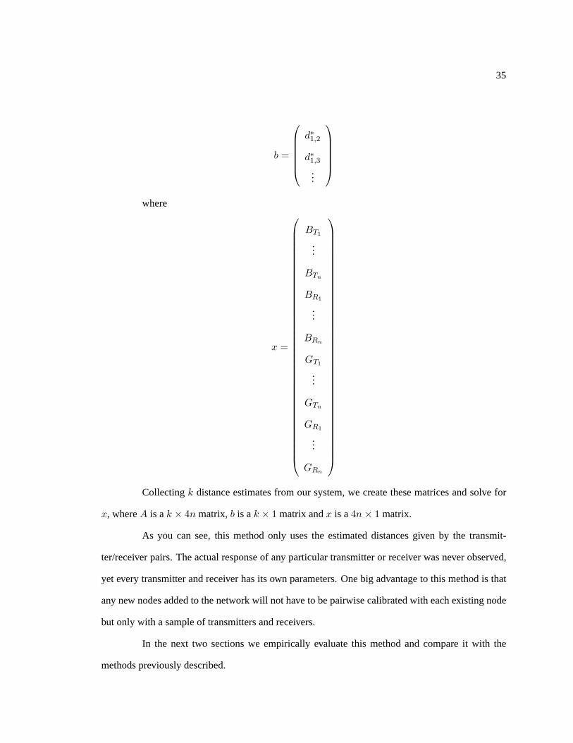
Collectingk distance estimates from our system, we create these matrices and solve for

x, whereA is ak × 4n matrix,b is ak × 1 matrix andx is a4n× 1 matrix.

As you can see, this method only uses the estimated distances given by the transmit-

ter/receiver pairs. The actual response of any particular transmitter or receiver was never observed,

yet every transmitter and receiver has its own parameters. One big advantage to this method is that

any new nodes added to the network will not have to be pairwise calibrated with each existing node

but only with a sample of transmitters and receivers.

In the next two sections we empirically evaluate this method and compare it with the

methods previously described.

36

0 50 100 150 200 2500

50

100

150

200

250

300

350

400

450

500

True Distance (cm)

Est

imat

ed D

ista

nce

(cm

)

Distance Estimates with Uniform Calibration

Figure 20: Uniform Calibration is essentially linear regression. It accounts for the fact thattransmit- and receive-delay exists, but does not account for the values of delay associated witheach transceiver.

7.3 Evaluation

For comparative purposes, we use linear regression to map the distance estimates to their

true distances in what we calluniform calibrationsince it characterizes all transmitters and receivers

in a uniform way with a single set of parameters, not accounting for individual variations among the

devices. The average error is 21% with uniform calibration, as seen in Figure 20.

In this section we evaluate and compare the three methods of parameter estimation: iter-

ative calibration, mean calibration, and joint calibration. To make the evaluations comparable, we

use the same parameters and calibration function in all cases and evaluate them using the same data.

Recall that our calibration function is

r∗ = BT + BR + GT × r + GR × r (0.15)

By convention, we will assume an uncalibrated node has parametersB = 0, G = 12 . This

37

gives us the reasonable model of two uncalibrated nodes:

r∗ = 0 + 0 +12× r +

12× r (0.16)

Iterative Calibration

For iterative calibration we chose an arbitrary node to be the reference transmitter, which

we call transmitterA, that we will use to calibrate all receivers. We assign it parametersBT = 0

andGT = 12 . Then, for each receiverR, we generate the matrices below with all distance estimates

d1, . . . , dk collected from transmitterA and receiverR. We then solve for the receiver parameters

BR andGR using least-squares.

x =

0

12

BR

GR

A =

1 d1 1 d1

1 d2 1 d2

......

......

1 dk 1 dk

b =

d∗1

d∗2...

d∗k

We then chose an arbitrary reference receiver which we call receiverB and use it to

calibrate all transmitters. This iteration is identical to the first except that we solve instead forBT

38

0 50 100 150 200 2500

50

100

150

200

250

300

350

400

450

500Iterative Calibration

Est

imat

ed D

ista

nce

(cm

)

True Distance (cm)

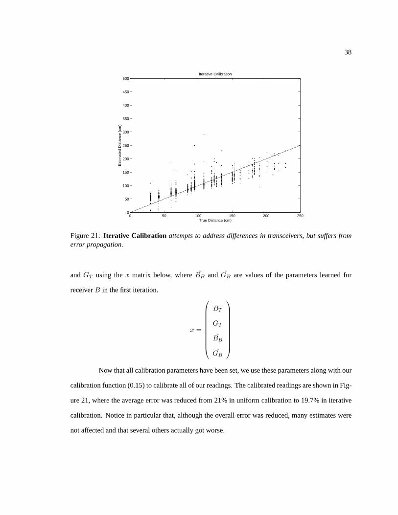
Figure 21: Iterative Calibration attempts to address differences in transceivers, but suffers fromerror propagation.

and GT using thex matrix below, whereBB and GB are values of the parameters learned for

receiverB in the first iteration.

x =

BT

GT

BB

GB

Now that all calibration parameters have been set, we use these parameters along with our

calibration function (0.15) to calibrate all of our readings. The calibrated readings are shown in Fig-

ure 21, where the average error was reduced from 21% in uniform calibration to 19.7% in iterative

calibration. Notice in particular that, although the overall error was reduced, many estimates were

not affected and that several others actually got worse.

39

0 50 100 150 200 2500

50

100

150

200

250

300

350

400

450

500

True Distance (cm)

Est

imat

ed D

ista

nce

(cm

)

Distance Estimates with Individual Calibration

Figure 22: Mean Calibration calibrates each receiver to the mean of all transmitters or eachtransmitter to the mean of all receivers. This approach works better than iterative calibration butdoes not allow one to calibrate both receivers and transmitters.

Mean Calibration

Mean calibration is identical to the first iteration in iterative calibration except that we use

all transmitters instead of just onestandardtransmitter. All transmitters are to remain uncalibrated,

so we assign them parametersBT = 0 andGT = 12 . For each receiverR, we generate the same

matrices as the first iteration of iterative calibration above but use the distance estimatesd1, . . . , dk

collected fromall transmitters and receiverR. We then solve for the receiver parametersBR and

GR using least-squares.

Having calibrated all receivers, we plot the calibrated distance estimates in Figure 22,

where the average error is reduced from 19.7% in iterative calibration to 16.0% in mean calibration.

40

0 50 100 150 200 2500

50

100

150

200

250

300

350

400

450

500

True Distance (cm)

Est

imat

ed D

ista

nce

(cm

)

Distance Estimates with Joint Calibration

Figure 23:Joint Calibration assigns parameters to each device such that overall system perfor-mance is optimized.

Joint Calibration

Using the method of joint calibration as described in Section 5, we obtain the results in

Figure 23, where the average error has been reduced from 16.0% in mean calibration to 10.1% in

joint calibration.

7.4 Distributed Parameter Management

Calamariuses distributed management of calibration parameters through what we call a

piggy-backingprotocol, where localization beacons are fundamentally tied to radio communication

packets. When a node sends a radio packet, it optionally also sends an acoustic pulse. There are

three advantages to this system. First, all radio messages are already time-stamped on arrival, giving

us a foundation for TOF readings at no additional cost. Second, since the RF range is larger than

the acoustic range, we don’t have beacon collision problems. If the beacon is accompanied by a

radio packet, we can identify the source; if it is not, there must have been a packet collision and

41

therefore potentially a beacon collision, so we ignore all acoustic information. The third advantage

to the piggy-backing protocol is that we do not have to worry about scheduling localization beacons.

We essentially hand the problem off to the wireless networking community; as they increase the

throughput of wireless networks, we automatically see more efficient beacon scheduling. Notice

that the corresponding disadvantage is that a communication-starved node is also location-starved.

Another benefit of using this piggy-backing protocol is efficient management of our cal-

ibration parameters. Each device maintains its own calibration parameters and sends them in the

payload of each localization beacon along with its current position estimate. Storing the parameters

in a distributed manner allows the network to change and grow dynamically with no overhead cost

for management or infrastructure. Furthermore, each node can autonomously adjust its own cali-

bration parameters over time, perhaps using techniques such as autocalibration as described in the

next section.

7.5 Autocalibration

The reason why joint calibration is so much more successful than iterative and mean cal-

ibration is that it used a more general parameter estimation technique where regression in the strict

sense failed. This method can in fact be extended to arbitrarily complex parameter estimation. One

such example is proposed in this section, where we frame calibration as a constrained optimization

problem.

In the previous sections, wemanuallycalibrated the devices in the sense that we had a

carefully controlled environment; we knew the true distance between each node. Let us define

autocalibration as calibration in anuncontrolled environment; we do not know the true distance

between each node.

Many sensor systems have incorporated an automatic calibration mechanism, perhaps for

the motors of a robotic arm [15] or for an electronic compass. However, autocalibration invariably

requires specialized hardware, such as the use of gyroscopes [11] or cameras.

42

Instead of using extra hardware in Calamari, we will usea priori information about local-

ization to try toinfer our device parameters.

The first piece ofa priori information is that in Calamari every transmitter/receiver pair

is also a receiver/transmitter pair. In other words, there are two distance estimates for each pair

of motes. One way to select parameters is to select those that maximize the consistency of the

responses between these symmetric pairs. This is to say, for nodesi andj, we want:

d∗ij = d∗ji (0.17)

whered∗ij = BTi + BRj + GTi × dij + GRj × dij ,

The second piece ofa priori information is that all distance estimates must satisfy the

triangle inequality. In other words, for any three nodesi, j, andk that are all connected:

d∗ij + d∗jk − d∗ik ≥ 0 (0.18)

Together, these two hooks into the problem give us a constrained optimization problem:

maximize consistency while satisfying the triangle inequality. To prevent the degenerate case where

all parameters equal zero, we must add two more terms to the objective function:∑

i(GTi −1)2 and

∑i(GRi − 1)2. A quadratic programming formulation arises:

Minimize:

∑

i<j

(d∗ij − dji∗)2 +∑

i

(GTi − 1)2 +∑

i

(GRi − 1)2

Subject to

d∗ij + d∗jk − d∗ik ≥ 0 ∀ trianglei,j,k

Notice that if we actually knew some distancedij , the known distance could easily replace

the estimated∗ij in the quadratic program above. This would allow us to easily take advantage of

anchor nodes or pre-calibrated nodes.

43

Furthermore, if we knew all distances this quadratic program would reduce to minimizing

the squared error between all distance estimates and their corresponding true distances. This would

effectively reduce the program to the least-squares approach used in joint calibration.

It is worthwhile to note that distance-based constraints were previously known to be useful

in the localization literature [3]. However, that paper differs from this work in that it maps out the

convex set of feasible locations for localization purposes whereas the constraints above map out the

convex set of feasible distances for calibration purposes.

8 The Localization Algorithm

In this section we describe the localization algorithm used in Calamari. We first briefly

consider the option of using centralized algorithms and review four existing distributed algorithms,

all of which approximate the distance between a node and an anchor using ashortest-pathtechnique.

This technique approximates the distance between two nodes to be the sum of the distances on

the shortest path through the network between them. Each node uses the approximate multi-hop

distance to the anchor nodes to estimate its own position.

Besides ranging errors, there are two new kinds of errors that the shortest-path technique

incurs. The first is caused by the fact that any process to find theshortest-path distance systemat-

ically prefers ranging estimates with negative errors. For this reason, multi-hop distance estimates

can be much shorter than expected. The second type of error arises from non-convexities in the

network, e.g. ahole in the network. Since shortest paths must go around this hole, many estimates

may be much longer than the true distance.

After reviewing several existing algorithms, we suggest a variant of the Ad-hoc Position-

ing System (APS) [19] that improves results between 20-30%. APS satisfies the design constraints

that the algorithm must be simple, approximate and scalable. With this modification, it also satisfies

the constraint that we achieve node-level resolution with the ranging errors we saw in Section 6.

We will be testing algorithms on random networks such as the one seen in Figure 24. In

44

Example of Simulated Network Topology

1

2 3

4

5

6

7 8

9

10

11

12

13 14

15 16

17

18 19

20 21

22

23 24

25

26 27

28

29

30

31

32 33

34

35

36

37 38

39

40 41

42 43

44

45

46 47

48

49

50

51

52 53

54

55

56

57

58 59

60 61

62

63 64

65

66

67 68

69

70 71

72

73

74 75

76

77

78

79

80

81 82

83 84

85 86

87

88

89

90

91

92

93 94

95

96 97

98 99

100

101

Figure 24:Example of Simulated Network TopologyNodes are placed pseudo-randomly. In thisdiagram, ’X’s indicate anchor nodes, black dots indicate mobile nodes and an edge indicates thata pair of nodes has a ranging estimate. In other diagrams, arrows indicate the positioning errorvector on the mobile nodes.

this diagram, ’X’s indicate anchor nodes, black dots indicate mobile nodes and an edge indicates

that a pair of nodes has a ranging estimate. In other diagrams, arrows indicate the positioning error

vector on the mobile nodes. To replicate the likely placement of nodes in a sensor network, nodes

are not placed completely randomly but are instead placed on a grid with large Gaussian noise equal

to the grid spacing on both theX andY axes, This results in fairly random graphs but avoids the

problem that large numbers of nodes are placed in a few very small regions, which is not likely in a

real sensor network deployment.

8.1 Existing Algorithms

Centralized Algorithms

Before exploring the many distributed algorithms, it is worthwhile to first consider the

realm of centralized algorithms. While no optimal ad-hoc localization algorithm exists as of yet,

45

many approximations could be used at a central node, such as multidimensional scaling [13], max-

imum likelihood methods [14], convex optimization [3], gradient descent, or even a global search

over all node configurations. The use of any such algorithm would of course require that all infor-

mation be sent to a central node which calculates the positions of all nodes. Those positions would

then be sent back to each node in the network, if necessary. This takesO(2nd) messages, wheren

is the number of nodes andd is the hop-diameter of the network. At the very least, this alternative

will give us a baseline by which to measure the bandwidth costs of distributed algorithms. In fact, it

is likely that every distributed algorithm can be partially characterized in terms of the diameter over

which that algorithm is cheaper than a centralized algorithm.

Bounding Box

Bounding Box methods define bounds on the coordinates of a mobile node in terms of

the estimated distance to each anchor node. Such methods are analyzed in [29] and used for initial

position estimation in Collaborative Multilateration, described below.

For any given nodei with distance estimatesdij to anchor nodesj, the coordinates ofi

are bounded according to

maxj(xj − dij) ≤ xi ≤ minj(xj + dij) (0.19)

maxj(yj − dij) ≤ yi ≤ minj(yj + dij) (0.20)

This can be easily extended to multi-hop networks wherej is not necessarily an anchor node. Let

xlbj andxub

j be the lower and upper bounds on nodej’s x coordinate. We have

maxj(xlbj − dij) ≤ xi ≤ minj(xub

j + dij) (0.21)

maxj(ylbj − dij) ≤ yi ≤ minj(yub

j + dij) (0.22)

A simple distributed algorithm arises where the only state information that each node

maintains is its own bounding box. The anchor nodes set their bounding box to be their known

positions and broadcast it. All other nodes update their state whenever a message is received and

46

broadcast their state whenever it changes. This algorithm requires no less thanO(and) messages,

wherea is the number of anchor nodes, since the position of each anchor node must reach every

other node. It also requires no more thanΩ(an2d) messages since each node in the network will

indirectly cause each other node to update a bounding box at most once.

While extremely simple, bounding box methods fail miserably when all mobile nodes are

not within the convex hull defined by the anchor nodes, as seen in Figure 25a. They also fail under

noisy range estimates; a single terribly small estimate can render the bounding box of all nodes

in the network inconsistent. However, as seen in Figure 26a, Bounding Box methods gracefully

degrade under non-convex networks because ranging estimates that are too large do not effect the

bounding box.

APS

Ad-hoc Positioning system (APS) as proposed in [19] is the natural extension of single-

hop multilateration to the multi-hop case. Similar to Bounding Box methods, APS approximates

the distance to each anchor node as the sum of distances over the multi-hop route to that anchor

node. Unlike Bounding Box methods, however, APS maintains these multi-hop distance estimates

explicitly and applies least-squares multilateration.

The distributed algorithm is exactly identical to the Bounding Box algorithm except that

the state each node maintains is the position of and the shortest-path distance to each anchor node.

Furthermore, after the shortest paths are found, each anchor node broadcasts acorrection factor

to help the other nodes deal with the systematic errors with the shortest-path technique that were

previously mentioned. These correction factors indicates the difference between multi-hop distances

that the anchor node has obtained through the shortest-path technique and the true distances that it

can calculate using its own known position.

While APS requires more state information, more network communication and more so-

phisticated local calculations than Bounding Box methods, it achieves reasonable position estimates

47

−1 −0.5 0 0.5 1 1.5 2 2.5 3 3.5 40

0.02

0.04Empirical Probability of Error (kernel smoothing)

Error (relative to maximum range)

Pro

babi

lity

1

2 3

4

5 6

7 8

9

10

11

12

13 14

15 16

17

18 19

20 21

22

23 24

25

26 27

28

29

30

31

32 33

34

35

36

37 38

39

40 41

42 43

44

45

46 47

48

49

50

51 52

53

54

55

56

57

58 59

60 61

62

63 64

65

66

67 68

69

70 71

72

73

74 75

76

77

78

79

80

81 82

83 84

85 86

87

88

89

90

91

92

93 94

95

96 97

98 99

100

101

Bounding Box

−0.1 0 0.1 0.2 0.3 0.4 0.5 0.6 0.7 0.80

0.02

0.04Empirical Probability of Error (kernel smoothing)

Error (relative to maximum range)

Pro

babi

lity

1

2 3

4

5 6

7 8

9

10

11

12

13 14

15 16

17

18 19

20 21

22

23 24

25

26 27

28

29

30

31

32 33

34

35

36

37 38

39

40 41

42 43

44

45

46 47

48

49

50

51 52

53

54

55

56

57

58 59

60 61

62

63 64

65

66

67 68

69

70 71

72

73

74 75

76

77

78

79

80

81 82

83 84

85 86

87

88

89

90

91

92

93 94

95

96 97

98 99

100

101

APS: DV−distance

Figure 25:Outside the Convex Hullof anchor nodes. Both figures are of identical networks withno noise added to range estimates. a) Bounding Box methods position all nodes within the convexhull b) APS can position nodes outside the convex hull.

48

−0.2 0 0.2 0.4 0.6 0.8 1 1.2 1.4 1.6 1.80

0.02

0.04Empirical Probability of Error (kernel smoothing)

Error (relative to maximum range)

Pro

babi

lity

1

2

3 4

5

6

7

8 9

10

11

12 13

14

15 16

17

18 19

20

21 22

23

24

25

26 27

28

29 30

31 32

33

34

35 36

37

38

39

40 41

42

43

44

45 46

47

48

49 50

51

52 53

54

55

56

57 58

59 60

61

62 63

64 65

66

67

68 69

70

71 72

73

74 75

76 77

78

79 80

81 82

83

84 85

86

87 88

89

90

91 92

93 94

95

96

97

98 99

100

101

102 103

104

105

Bounding Box

−0.5 0 0.5 1 1.5 2 2.50

0.02

0.04Empirical Probability of Error (kernel smoothing)

Error (relative to maximum range)

Pro

babi

lity

1

2

3 4

5

6

7

8 9

10

11

12 13

14

15 16

17

18 19

20

21 22

23

24

25

26 27

28

29 30

31 32

33

34

35 36

37

38

39

40 41

42 43

44

45 46

47

48

49 50

51

52 53

54

55

56

57 58

59 60

61

62 63

64 65

66

67 68 69

70

71 72

73

74 75

76 77

78

79 80

81 82

83

84 85

86 87

88

89

90

91 92

93 94

95

96

97

98 99

100

101

102 103

104

105

APS: DV−distance

Figure 26: Non-convex Topologycauses systematic error in multi-hop distance estimates. Bothfigures are of identical networks with no noise added to range estimates. a) Bounding Box methodsare fairly robust to non-convex topologies b) APS sees large degradation.

49

even when all mobile nodes are not within the convex hull defined by the anchor nodes, as seen in

Figure 25b. It is also more robust to noise than Bounding Box methods because the effect of a single

erroneous reading is outweighed by the other distance estimates. However, Figure 26b shows that

APS does not show the same graceful degradation under non-convex and ill-constraining network

topologies seen in Bounding Box methods because estimates that are much too large badly effect

multilateration results.

Collaborative Multilateration

Collaborative Multilateration as proposed in [26] uses Bounding Box methods for initial

position estimates, which are then shared with all local neighbors. This information, along with local

range estimates, is then used to achieve a new position estimate using least squares multilateration.

Each node then broadcasts its new position to all neighbors, who again use it to update their own

positions. This process iterates until the position estimates converge.

Clearly, this process is not guaranteed to converge; a single extremely erroneous initial

position estimate could pull other nodes further from their true positions. To prevent this from

happening, this algorithm first definescollaborative subtreeswhich are sets of nodes whose possible

positions are well-defined. The iterative process is then run only on these subtrees and the refined

positions are later used to update the positions of the other nodes. This prevents nodes with ill-

defined positions from adversely effecting the iterative process.

The iterative process described above is in effect one of many possible gradient descent

methods, which seem not to require any global information at all. Global information is being

propagated slowly with each iteration, however, and the convergence time will therefore depend

indirectly on the distance to the nearest anchor nodes. The method used by Savvides [26] was seen

to converge in approximately one hundred iterations with one hundred nodes. One is unable to

accurately predict the exact bandwidth cost of iterative algorithms, but it is clearlyΩ(nd) and, as

seen from this data, likely to be equal to or better thanO(n2).

50

hop-TERRAIN/Refinement

Hop-TERRAIN/Refinement as proposed in [25] is similar to Collaborative Multilatera-

tion in the sense that it uses multi-hop distances to achieve initial position estimates and a gradient

ascent method to refine those estimates. One important difference is that this algorithm uses APS to

achieve initial positions instead of Bounding Box methods, which we have seen to perform poorly

under certain conditions. The gradient descent method is very similar to that seen in Collaborative

Multilateration in the sense that multilateration is performed on the current position estimates of

a node’s neighbors. However, instead of defining collaborative subtrees, this algorithm usescon-

fidencevalues on each node’s position. Confidence originates at an anchor node and propagates

through the network along with the effect of that node’s position information. The cost, accuracy

and running time analysis of this algorithm is therefore roughly comparable to Collaborative Multi-

lateration except that it does not pay the cost of building collaborative subtrees.

8.2 Resolution of Forces

Of the four distributed algorithms mentioned above, APS appears to best meet the design

constraints of Calamari. While much cheaper in terms of bandwidth and computation than both

Collaborative Multilateration and hop-TERRAIN/Refinement, it does not suffer from the robustness

problems of Bounding Box methods. Furthermore, results from [19, 25] indicate that position errors

are reasonable, i.e. less than the connectivity range, even with distance error rates up to 50%. Here,

we further analyze this algorithm and propose a variant that can reduce error rates between 20% and

30%. We will focus on theDV-distance algorithm proposed with APS in [19].

Figure 27a shows position estimates from APS on a convex, isotropic network contained

within the convex hull of anchor nodes. While this is an ideal network under the specifications

of APS, there is clearly systematic error in the position estimates caused by the shortest-path phe-

nomenon; since many multi-hop distance estimates are too short, most positions are too close to the

center of the network. Figure 26b shows the opposite problem where the network is non-convex and

51

−0.1 0 0.1 0.2 0.3 0.4 0.5 0.6 0.7 0.80

0.02

0.04Empirical Probability of Error (kernel smoothing)

Error (relative to maximum range)

Pro

babi

lity

1

2

3 4 5

6

7 8

9

10

11 12

13

14 15

16 17

18

19 20

21

22 23

24

25 26

27

28

29

30 31

32

33

34

35 36

37 38

39

40

41 42

43

44

45

46

47

48

49

50 51

52

53

54

55 56 57

58 59 60

61 62

63

64 65

66

67 68 69

70 71

72 73

74

75

76

77

78

79

80 81

82 83

84

85 86

87

88 89

90

91

92

93

94

95

96 97 98

99

100

101 102

103 104

105

106

107 108

109

110 111

112

113 114

115 116

117

118 119

120

121 122

123

124

125 126

127

128 129 130

131 132

133

134

135

136 137

138 139

140

141

142

143

144

145 146

147 148

149 150

151 152

APS: DV−distance

−0.1 0 0.1 0.2 0.3 0.4 0.5 0.6 0.7 0.80

0.02

0.04Empirical Probability of Error (kernel smoothing)

Error (relative to maximum range)

Pro

babi

lity

1

2

3 4 5

6

7 8

9

10

11 12

13

14 15

16 17

18

19 20

21

22 23

24

25 26

27 28

29

30 31

32

33

34

35 36

37 38

39

40

41 42

43

44

45 46

47

48

49

50 51

52

53

54

55 56 57

58 59 60

61 62

63

64 65

66

67 68 69

70 71

72 73

74

75

76

77

78

79

80 81

82 83

84

85 86

87

88 89

90

91

92

93

94

95

96 97 98

99

100

101 102

103 104

105

106

107 108

109

110 111

112

113 114

115 116

117

118 119

120

121 122

123

124

125 126

127

128 129 130

131 132

133

134

135

136 137

138 139

140

141

142 143

144

145 146

147 148

149 150

151 152

Resolution of Forces

Figure 27: Convex, Isotropic Topologyreveals systematic error in the shortest-path technique.Both figures are of identical networks with N(0,15%) noise. a) APS positions most nodes too closeto the center b) Resolution of Forces is not as largely affected.

52

multi-hop distance estimates are too long.

APS’s anchor-node correction factor reduces overall error but does not eliminate the sys-

tematic error seen in Figures 27a and 26b. The reason for this error is that standard multilateration

techniques penalize the squared error(dij− dij)2 wheredij is the observed distance between nodei

andj anddij is the calculated distance given the position estimates. However, minimizing squared

error is only optimal only if the distance errors are Normally distributed.

Laplace(X, α, β) =12β

e− |X−α|

β (0.23)

Normal(X,µ, σ) =1√2πσ

e−12(X−α

σ )2

(0.24)

The Laplace density function 0.23 is identical to that of the Normal distribution 0.24

except that it decreases with absolute error instead of squared error. Figure 28 shows the error

distribution of multi-hop distance estimates with a Gaussian and Laplace fit. Clearly, the error’s

highly-peaked, heavy tailed distribution is better approximated by the Laplace Distribution than the

Gaussian, requiring minimization of absolute error instead of squared error.

To do this, we will use a simple technique that resolves theforceon each node by each

anchor node, a technique we will call Resolution of Forces. Given an initial position estimate, some

amount of error will be associated with each anchor node. This error is like a force in the sense

that it has a magnitude and direction. Minimizing absolute error amounts to making the sum of all

forces be equal to zero, which is done by simply moving the position estimate to the current position

plus the resultant of all the forces. Resolution of Forces, therefore, is a very simple technique that

requires an initial estimate and runs inO(a) time, wherea is the number of anchor nodes. For initial

position estimates, this algorithm uses Bounding Box methods if possible, which are extremely

simple. If the bounding box is inconsistent or the error is too high after the first iteration, the second

iteration uses least squares multilateration similar to APS, and then refines these estimates using

Resolution of Forces. A similar method to LMS, which is used in least-squares multilateration, is

53

−4 −3.5 −3 −2.5 −2 −1.5 −1 −0.5 0 0.50

0.2

0.4

0.6

0.8

1

1.2

1.4

1.6

1.8Multi−hop Distance Error Distribution

Distance Estimate Error (relative to maximum range)

Emprical DistributionNormal FitLaplace Fit

Figure 28:Multi-hop Distance Error Distribution is highly-peaked and heavy-tailed, more closelyresembling a Laplace distribution than a Normal Distribution.

being developed that will minimize absolute error without the need of an initial position estimate.

Figure 27b shows the position error distribution using Resolution of Forces on the same

network as in Figure 27. Looking at the error distributions at the tops of the figures reveals that

the errors that were reduced were those with the greatest magnitude. This fact corroborates our

explanation that this method works better because of the heavy-tailed error distribution; squared

error magnifies the effect of large errors in the tails. In this case, average error was reduced by

23%. Resolution of Forces also improves results in more poorly defined networks. Figure 29 shows

Resolution of Forces on the networks from Figures 25 and 26. In these cases, error was reduced by

22% and 26% respectively.

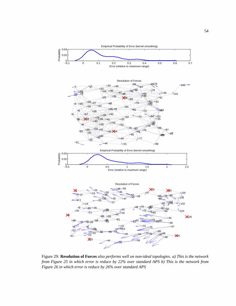
54

−0.1 0 0.1 0.2 0.3 0.4 0.5 0.6 0.70

0.02

0.04Empirical Probability of Error (kernel smoothing)

Error (relative to maximum range)

Pro

babi

lity

1

2 3

4

5 6

7 8

9

10

11

12

13 14

15 16

17

18 19

20 21

22

23 24

25

26 27

28

29

30

31

32 33

34

35

36

37 38

39

40 41

42 43

44

45

46 47

48

49

50

51 52

53

54

55

56

57

58 59

60 61

62

63 64

65

66

67 68

69

70 71

72

73

74 75

76

77

78

79

80

81 82

83 84

85 86

87

88

89

90

91

92

93 94

95

96 97

98 99

100

101

Resolution of Forces

−0.5 0 0.5 1 1.5 2 2.50

0.02

0.04Empirical Probability of Error (kernel smoothing)

Error (relative to maximum range)

Pro

babi

lity

1

2

3 4

5

6

7

8 9 10

11

12 13

14

15 16

17

18 19

20

21 22

23

24

25

26 27

28

29 30

31 32

33

34

35 36

37

38

39

40 41

42 43

44

45 46

47

48

49 50

51

52 53

54

55

56

57 58

59 60

61

62 63

64 65

66

67 68 69

70

71 72

73

74 75

76 77

78

79 80

81 82

83

84 85

86 87

88

89

90

91 92

93 94

95

96 97

98 99

100

101

102 103

104

105

Resolution of Forces

Figure 29:Resolution of Forcesalso performs well on non-ideal topologies. a) This is the networkfrom Figure 25 in which error is reduce by 22% over standard APS b) This is the network fromFigure 26 in which error is reduce by 26% over standard APS

55

9 Software Architecture

In this section we describe the software architecture of Calamari. Calamari is being in-

tegrated into theZ-Racerapplication as a part of the DARPA NEST project acknowledged below.

Because this is a collaborative project involving more than a dozen different groups, one main ob-

jective is to “provide a framework to allow Middleware providers to develop individual components

in a reasonably independent manner” [28]. In this section we try to obtain that goal by defining a

modular and composable set of localization subsystems with well-defined APIs.

Defining a composable architecture is advantageous for more than simply facilitating col-

laboration among independant groups. It also helps support extensions and improvements to the

system. For example, it is likely that ad-hoc ranging technology will improve dramatically in a

matter of years and that new distributed localization algorithms will be developed. The architecture

defined below allows one to easily exploit new technology as it becomes available.

Calamari, along with the rest of theZ-Racerapplication, is being implemented in NesC,

a language designed for network embedded technology [5]. NesC applications consists of several

softwarecomponentswhich exposeinterfacesand arewired together much like hardware compo-

nents might be. This architecture will therefore be articulated in terms of the functionality of the

components, their interfaces, and a wiring diagram.

System Overview

The overall system can be viewed as a three-layer system as shown in Figure 30. The

bottom layers interface the system with the physical world. The middle layer acts as a data bridge

between the bottom and top layers, both within the same mote and between motes. The top layer

uses information from the bottom layer and from other nodes in the network to infer location in

cartesian space. The control of each subsystem and the availability of data is exposed to the appli-

cation as a single interface. The following sections describe the three sub-systems individually; for

a more detailed description of the data structures and interface definitions, see [28].

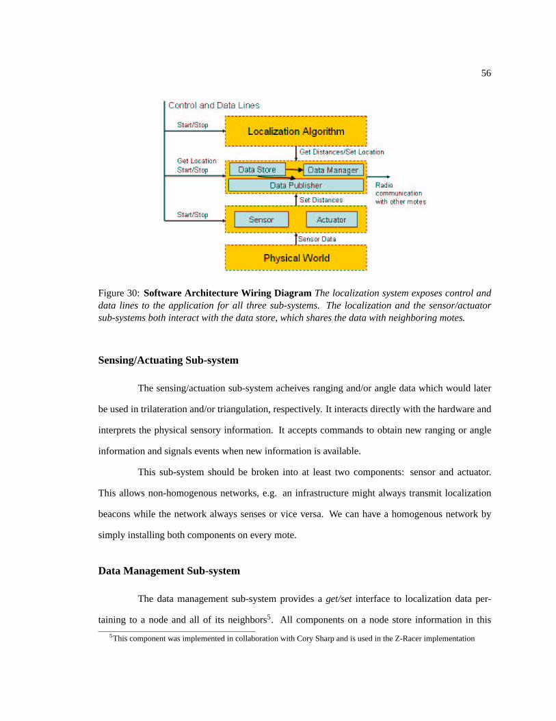
56

Figure 30:Software Architecture Wiring Diagram The localization system exposes control anddata lines to the application for all three sub-systems. The localization and the sensor/actuatorsub-systems both interact with the data store, which shares the data with neighboring motes.

Sensing/Actuating Sub-system

The sensing/actuation sub-system acheives ranging and/or angle data which would later

be used in trilateration and/or triangulation, respectively. It interacts directly with the hardware and

interprets the physical sensory information. It accepts commands to obtain new ranging or angle

information and signals events when new information is available.

This sub-system should be broken into at least two components: sensor and actuator.

This allows non-homogenous networks, e.g. an infrastructure might always transmit localization

beacons while the network always senses or vice versa. We can have a homogenous network by

simply installing both components on every mote.

Data Management Sub-system

The data management sub-system provides aget/setinterface to localization data per-

taining to a node and all of its neighbors5. All components on a node store information in this

5This component was implemented in collaboration with Cory Sharp and is used in the Z-Racer implementation

57

component and it is automatically shared with the data managers running on neighboring nodes.

When a component on one node needs information that originated in a different component or on a

different mote, it uses a simplegetinterface. This component vastly simplifies data sharing between

components and over the radio. Furthermore, by consolidating the radio protocol and software API

for data sharing into a single component, coupling between the remaining components is reduced

and so composability of components is increased.

This sub-system should be broken into at least three subcomponents: the data store, the

data-sharing manager, and the membership manager. The data store is responsible for storing and

retrieving data efficiently. The data-sharing manager is responsible for sharing data over the radio.

This abstraction is necessary because each application may want a different protocol for shared data,

e.g. sharing lazily, eagerly, lossily, enforcing consistency, etc. The membership manager decides

which nodes are in one’s neighborhood. This abstraction is necessary because each application may

want a different set of neighbors. For example, a routing component may want the neighbors with

the best radio link while localization may want to the neighbors with the most accurate ranging

information.

Localization Sub-system

The localization sub-system uses information from other nodes and from the sensing/actuating

sub-system to estimate the node location. For example, using its neighbors’ position estimates and

ranging estimates obtained through the sensing/actuating sub-system, the node’s own position can

be estimated using simple multilateration. Or, using its neighbors’ estimated distances to anchor

nodes and ranging estimates, the node’s own position can be estimated using APS. Once the po-

sition is estimated, it is stored in the data management sub-system and thereby shared with all

neighbors.

58

Control Interface

The localization system exposes a control interface to the application by which all sub-

systems are controlled. Control should be separate from the other systems because usage of local-

ization is almost completely defined by the application. For example, in a static environment the

system might only localize once in the beginning of the application and then never again. If some-

thing walks into a room the system might want all nodes near the moving node to help it localize.

In a completely dynamic environment the system might want all nodes constantly localizing by

following a scheduling algorithm.

As well as decomposing the localization system into functional components, this archi-

tecture also decomposes the system in terms costs and benefits. For example, one could improve

spatial resolution by repeatedly using the sensor/actuator sub-system, at the cost of power. One

could improve temporal resolution by repeatedly using the localization sub-system, at the cost of

cpu cycles. One could increase the data-update frequency in a mobile network by repeatedly syn-

chronizing the data manager sub-systems, at the cost of network bandwidth. Because the control of

the system is exposed as an external interface, such tradeoff decisions can be made specific to the

needs and resources of each application.

10 Experimental Validation

Having defined the three main components of Calamari, we must empirically evaluate the

system. In this section we describe the exact hardware and methodology used to collect data and

some preliminary experiments used to evaluate this localization system.

Calamari is built on the MICA sensor platform [10]. The MICA mote is essentially an

Atmel 103 micro-controller in conjunction with a RFM TR1000 radio transceiver and is about the

size of two AA batteries, as seen in Figure 32. Connected to each mote is a MICA sensor board [33]

which, among other things, contains a Sirius PS14T40A 4.3KHz sounder and a Panasonic WM-

59

Figure 31:Experimental Testbedconsists of a 8 x 4 grid of 32 nodes at 30cm spacing

62A microphone, whose band-passed output is wired to a National Semiconductor LMC567CM

tone detector whose center frequency is set to about 4.5KHz.

In our experiments we use 32 nodes in a 30cm x 30cm grid. The motes are situated atop

a large table in an 8 x 4 formation spanning a total area of 210cm x 90cm, as seen in Figure 31. All

motes are in the same orientation. Both the sounder and microphone point directly upwards. The

sounder is located in the center of the board while the microphone is in one corner, as seen in Figure

32.

Although this experimental setup does not test all combinations of paired distances and

relative orientations, it does provide a nice sampling of that space. A total of 24 distances ranging

from 30cm to 210cm are measured using this setup. While all motes are in the same orientation

on the table, they are not all in the same orientation relative to each other. A total of 992 trans-

mitter/receiver pairs are used, although each at only one distance and orientation. The acoustic

transmission frequencies are distributed evenly from 4.2KHz to 4.5KHz while the tone detector

center frequencies are distributed between 4.4KHz and 4.6KHz.

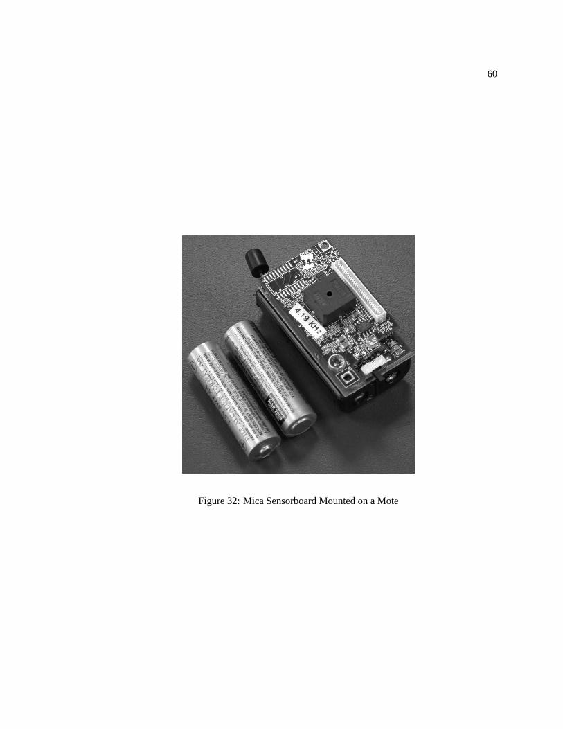
60

Figure 32: Mica Sensorboard Mounted on a Mote

61

To generate the data, each transmitter sent several localization beacons allowing all other

nodes to make a single distance estimate. Each node therefore generated up to 31 distance estimates,

which were seen for Joint Calibration in Figure 23. Not all pairs of nodes were able to make distance

estimates and node number eight did not generate any data in any of the experiments. In the first

experiment, to create a multi-hop scenario, all distances estimates of more than one node spacing

were ignored in this experiment. In the second experiment, to test how results vary as network

density varies, the node density was doubled while the range remained the same.

Three anchor nodes were placed in the network such that approximately 50% of the nodes

were contained within the convex hull that they defined. All nodes were calibrated according to

Section 7 and each node positioned itself using the techniques presented in Section 8.2.

The resulting error was on the order of the node density for both experiments and the

resulting positions are shown in Figure 33. As we can see, we can achieve node-level resolution us-

ing this ranging methodology and localization algorithm. Furthermore, accuracy increases as node

density increases. This is a very desirable property that is not achieved through infrastructure-based

localization systems such as GPS. It effectively uses the high network density as an advantage to

increase resolution, ensuring that the user can always observe the spatial frequency desired. An

intuitive explanation for this is that higher node densities reduce the non-convexities in the network,

i.e. multi-hop distances more closely approximate a straight-line distance. These preliminary ex-

periments have served as a proof-of-concept for Calamari and are motivating more experiments in

the future.

11 Conclusion

Every application has different goals and every problem domain imposes new constraints

on system design. As we have seen, localization is unfortunately ahard problem in the sense

that subtly different goals or constraints have historically resulted in drastically different designs of

localization systems. Calamari was designed specifically for the localization goals and constraints of

62

−0.1 0 0.1 0.2 0.3 0.4 0.5 0.6 0.7 0.80

0.02

0.04Empirical Probability of Error (kernel smoothing)

Error (relative to maximum range)

Pro

babi

lity

4

5

7

10

15

16 17

18

22

23

26

28

29

30 31

32

Resolution of Forces

−0.1 0 0.1 0.2 0.3 0.4 0.5 0.6 0.70

0.02

0.04Empirical Probability of Error (kernel smoothing)

Error (relative to maximum range)

Pro

babi

lity

1

2

3 4

5

6

7 9

10 11

12

13

14

15

16 17

18

19

20

21 22

23 24

25 26

27

28

29

30 31

32

Resolution of Forces

Figure 33:Experimental Resultsa) a low density network exhibits node-level resolution. b) Whenthe density is doubled, resolution increases due to thestraighteningof shortest paths.

63

typical sensor network applications such as Z-Racer: simple design, node-level resolution, scalable

deployment, and event-driven operation.

Calamari is an extremely simple system. All nodes use identical hardware and run identi-

cal algorithms and, unlike systems like GPS or Cricket, Calamari does not require precise infrastruc-

tural support. Because localization must only be approximate in sensor networks, both hardware

and computational costs are reduced from comparable systems like AHLoS that aim to achieve

much higher accuracy.

Because the localization algorithm only works within convex regions of the network,

Calamari requires at least three anchor nodes in each such convex region. For example, indoors

this would require at least three anchor nodes in each room, which is not a large improvement over

systems like Cricket. However, Calamari’s deployment time scales extremely well in large spaces

such as warehouses or outdoors. Whereas systems like Cricket require at least three anchor nodes

to be within ten meters of every position, Calamari requires only three anchor nodes in the entire

region.

Because sensor nodes are typically stationary, Calamari is event driven. Ranging and

localization in the system as a whole are triggered only by the introduction of each new anchor

node. As new mobile nodes enter the network, they can request ranging and location information

from their neighbors. This protocol complies with the low duty-cycle power-saving strategy often

used in sensor networks.

Calamari was able to take advantage of several unique properties of wireless sensor net-

work localization, including the fact that nodes are mostly stationary and the fact that nodes are

quite numerous and must be relatively near each other to form a network. While Calamari has paid

for its minimalistic design with accuracy and resolution, it is still able to achieve the node-level

resolution required by many sensor network applications.

64

Acknowledgements

This work is funded in part by the National Defense Science and Engineering Graduate

Fellowship, the DARPA NEST contract F33615-01-C-1895, and Intel Research.

65

Bibliography

[1] Paramvir Bahl and Venkata N. Padmanabhan. RADAR: An in-building RF-based user location

and tracking system. InINFOCOM (2), pages 775–784, March 2000.

[2] R. Barrett, M. Berry, and T. F. Chan et al. Templates for the solution of linear systems:

Building blocks for iterative methods. InSIAM, Philadelphia, 1994.

[3] L. Doherty and et al. Convex position estimation in wireless sensor networks. InInfocom, Los

Alamitos, Calif., 2001. IEEE CS Press.

[4] Deepak Ganesan, Bhaskar Krishnamachari, Alec Woo, David Culler, Deborah Estrin, and

Stephen Wicker. Complex behavior at scale: An experimental study of low-power wireless

sensor networks. UCLA Computer Science Technical Report UCLA/CSD-TR 02-0013.

[5] David Gay, Phil Levis, Rob von Behren, Matt Welsh, Eric Brewer, and David Culler. The nesc

language: A holistic approach to networked embedded systems. InProgramming Language

Design and Implementation (PLDI), San Diego, June 2003.

[6] E. N. Gilbert. Random plane networks.Journal of SIAM, 9:533–543, 1961.

[7] Andy Harter, Andy Hopper, Pete Steggles, Andy Ward, and Paul Webster. The anatomy of a

context-aware application. InMobile Computing and Networking, pages 59–68, 1999.

[8] Jeffrey Hightower and Gaetano Borriello. Location systems for ubiquitous computing.IEEE

Computer, 34(8):57–66, August 2001.

66

[9] Jeffrey Hightower, Chris Vakili, Gaetano Borriello, and Roy Want. Design and calibration of

the spoton ad-hoc location sensing system. August 2001.

[10] Jason Hill, Robert Szewczyk, Alec Woo, Seth Hollar, David E. Culler, and Kristofer S. J.

Pister. System architecture directions for networked sensors. InACM ASPLOS IX, November

2000.

[11] Bruce Hoff and Ronald Azuma. Autocalibration of an electronic compass in an outdoor aug-

mented reality system. InIEEE and ACM International Symposium on Augmented Reality,

pages 159–164, Munich, Germany, October 2000.

[12] B. Hofmann-Wellenho, H. Lichtenegger, and J.Collins.Global Positioning System: Theory

and Practice. Springer Verlag, fourth edition, 1997.

[13] Joseph B. Kruskal and Myron Wish.Multidimensional Scaling. Sage Publications, Inc., 1978.

[14] et. al Luis Navarro-Serment. A beacon system for the localization of distributed robotic teams.

In the International Conference on Field and Service Robotics, Pittsburgh, PA, August 1999.

[15] D. Ma and J. M. Hollerbach. Identifying mass parameters for gravity compensation and au-

tomatic torque sensor calibration.IEEE Intl Conf Robotics and Automation, pages 661–666,

April 1996.

[16] Alan Mainwaring, Joseph Polastre, Robert Szewczyk, David Culler, and John Anderson. Wire-

less sensor networks for habitat monitoring.ACM International Workshop on Wireless Sensor

Networks and Applications (WSNA), September 2002.

[17] James McLurkin. Algorithms for distributed sensor networks. Master’s thesis, University of

California at Berkeley, 1999.

[18] Mouser. Microphone elements, transducers, and earphones specification sheet.

http://www.mouser.com/catalog/612/633.pdf, Nov-Feb 2002. Catalog 612.

67

[19] Dragos Niculescu and Badri Nath. Ad hoc positioning system (APS). InGLOBECOM (1),

pages 2926–2931, 2001.

[20] C. C. Paige and M. A. Saunders. LSQR: An algorithm for sparse linear equations and sparse

least squares.ACM Trans. Math. Soft., 8:43–71, 1982.

[21] PinPoint. Pinpoint home page. http://www.rftechnologies.com/pinpoint/.

[22] Nissanka B. Priyantha, Anit Chakraborty, and Hari Balakrishnan. The cricket location-support

system. InMobile Computing and Networking, pages 32–43, 2000.

[23] Raab, Blood, Steiner, and Jones. Magnetic position and orientation tracking system.IEEE

Transactions on Aerospace and Electronic Systems, AES-15(5), September 1979.

[24] RFM. Rfm tr1000 transceiver specifications. http://www.rfm.com/products/data/tr1000.pdf.

[25] Chris Savarese. Robust positioning algorithms for distributed ad-hoc wireless sensor networks.

Master’s thesis, University of California at Berkeley, 2002.

[26] A. Savvides, H. Park, and M. B. Srivastava. The bits and flops of the n-hop multilateration

primitive for node localization problems. InFirst ACM International Workshop on Sensor

Networks and Applications, Septmber 2002.

[27] Andreas Savvides. Ahlos hardware webpage. http://nesl.ee.ucla.edu/projects/ahlos/hardware.htm.

[28] Cory Sharp and NEST group. Network embedded software technology tracking minitask ar-

chitecture document. http://cvs.sourceforge.net/cgi-bin/viewcvs.cgi/tinyos/minitasks/02/doc/.

[29] Slobodan Simic. A distributed algorithm for localization in random wireless networks. sub-

mitted to Discrete Applied Mathematics, 2002.

[30] SyChip. Sychip gps module. http://www.sychip.com/gps-module.html.

68

[31] R. Want, A. Hopper, V. Falcao, and J. Gibbons. The active badge location system.ACM

Transactions on Information Systems, 40, January 1992.

[32] WhereNet. Wherenet home page. http://www.wherenet.com.

[33] Alec Woo. Mica sensor board. http://today.cs.berkeley.edu/tos/hardware/hardware.html.