Embed Size (px)
Citation preview

Computer Science II
Course at D-BAUG, ETH Zurich
Felix Friedrich & Hermann Lehner
SS 2019
1

Welcome!Course homepage
http://lec.inf.ethz.ch/baug/informatik2/2019/
The team:Lecturers Felix Friedrich
Hermann LehnerAssistants Patrick Gruntz
Aristeidis MastorasChris WendlerManuel Winkler
Back-office Katja Wolff
2

ExercisesMon Tue Wed Thu Fri Sat Sun Mon Tue Wed Thu Fri Sat
issuance preliminary discussionsubmission
discussion
V Ü V Ü
Exercises availabe at lectures.Preliminary discussion in the following recitation sessionSolution of the exercise until two days before the next recitation session.Dicussion of the exercise in the next recitation session.
3

ExercisesThe solution of the weekly exercises is voluntary but stronlyrecommended.
4

It is so simple!
For the exercises we use an online development environment thatrequires only a browser, internet connection and your ETH login.
If you do not have access to a computer: there are a a lot of computers publiclyaccessible at ETH.
5

Literature
Algorithmen und Datenstrukturen, T. Ottmann, P. Widmayer,Spektrum-Verlag, 5. Auflage, 2011
Algorithmen - Eine Einführung, T. Cormen, C. Leiserson, R.Rivest, C. Stein, Oldenbourg, 2010
Introduction to Algorithms, T. Cormen, C. Leiserson, R. Rivest, C.Stein , 3rd ed., MIT Press, 2009
Algorithmen Kapieren, Aditya Y. Bhargava, MITP, 2019.
6

Exams
The exam will cover
Lectures content (lectures, handouts)
Exercise content (recitation hours, exercise tasks).
Written exam.
We will test your practical skills (algorithmic and programming skills) andtheoretical knowledge (background knowledge, systematics).
7

Offer
Doing the weekly exercise series→ bonus of maximally 0.25 of agrade points for the exam.The bonus is proportional to the achieved points of speciallymarked bonus-task. The full number of points corresponds to abonus of 0.25 of a grade point.The admission to the specially marked bonus tasks can dependon the successul completion of other exercise tasks. The achievedgrade bonus expires as soon as the course has been given again.
8

Offer (concretely)
3 bonus exercises in total; 2/3 of the points suffice for the exambonus of 0.25 marksYou can, e.g. fully solve 2 bonus exercises, or solve 3 bonusexercises to 66% each, or ...Bonus exercises must be unlocked (→ experience points) bysuccessfully completing the weekly exercisesIt is again not necessary to solve all weekly exercises completelyin order to unlock a bonus exerciseDetails: exercise sessions, online exercise system (Code Expert)
9

Academic integrity
Rule: You submit solutions that you have written yourself and thatyou have understood.
We check this (partially automatically) and reserve our rights toadopt disciplinary measures.
10

Exercise group registration IVisit http://expert.ethz.ch/enroll/SS19/ifbaug2Log in with your nethz account.
11

Exercise group registration IIRegister with the subsequent dialog for an exercise group.
12

Overview
13

Programming Exercise
A: compileB: runC: test
D: descriptionE: History
14

Test and Submit
Test
Submission
15

Where is the Save Button?
The file system is transaction based and is saved permanently(“autosave”). When opening a project it is found in the most recentobserved state.The current state can be saved as (named) snaphot. It is alwayspossible to return to saved snapshot.The current state can be submitted (as snapshot). Additionally,each saved named snapshot can be submitted.
16

Snapshots
Look at snapshot
Submission
Go Back
17

Should there be any Problems ...
with the course content
definitely attend all recitation sessionsask questions thereand/or contact the assistant
further problems
Email to lecturer (Felix Friedrich, Hermann Lehner)
We are willing to help.
18

1. Introduction
Algorithms and Data Structures, Correctness, a First Example
19

Goals of the course
Understand the design and analysis of fundamental algorithmsand data structures.Understand how an algorithmic problem is mapped to asufficiently efficient computer program.
20

Contents
data structures / algorithmsThe notion invariant, cost model, Landau notation
algorithms design, inductionsearching, selection and sorting
dictionaries: hashing and search trees, balanced treesdynamic programming
fundamental graph algorithms, shortest paths, maximum flow
Software EngineeringPython Introduction
Python Datastructures
21

1.1 Algorithms
[Cormen et al, Kap. 1;Ottman/Widmayer, Kap. 1.1]
22

Algorithm
Algorithm: well defined computing procedure to compute output datafrom input data
23

example problem
Input: A sequence of n numbers (a1, a2, . . . , an)Output: Permutation (a′1, a
′2, . . . , a
′n) of the sequence (ai)1≤i≤n, such that
a′1 ≤ a′2 ≤ · · · ≤ a′n
Possible input(1, 7, 3), (15, 13, 12,−0.5), (1) . . .
Every example represents a problem instance
The performance (speed) of an algorithm usually depends on theproblem instance. Often there are “good” and “bad” instances.
24

Examples for algorithmic problems
Tables and statistis: sorting, selection and searchingrouting: shortest path algorithm, heap data structureDNA matching: Dynamic Programmingevaluation order: Topological Sortingautocomletion and spell-checking: Dictionaries / TreesFast Lookup : Hash-TablesThe travelling Salesman: Dynamic Programming, MinimumSpanning Tree, Simulated Annealing
25

Characteristics
Extremely large number of potential solutionsPractical applicability
26

Data Structures
A data structure is a particular way oforganizing data in a computer so thatthey can be used efficiently (in thealgorithms operating on them).Programs = algorithms + datastructures.
27

Efficiency
Illusion:
If computers were infinitely fast and had an infinite amount ofmemory ...... then we would still need the theory of algorithms (only) forstatements about correctness (and termination).
Reality: resources are bounded and not free:
Computing time→ EfficiencyStorage space→ Efficiency
Actually, this course is nearly only about efficiency.28

2. Efficiency of algorithms
Efficiency of Algorithms, Random Access Machine Model, FunctionGrowth, Asymptotics [Cormen et al, Kap. 2.2,3,4.2-4.4 |Ottman/Widmayer, Kap. 1.1]
29

Efficiency of Algorithms
Goals
Quantify the runtime behavior of an algorithm independent of themachine.Compare efficiency of algorithms.Understand dependece on the input size.
30

Programs and Algorithms
program
programming language
computer
algorithm
pseudo-code
computation model
implemented in
specified for
specified in
based on
Technology Abstraction
31

Technology Model
Random Access Machine (RAM)
Execution model: instructions are executed one after the other (onone processor core).Memory model: constant access time (big array)Fundamental operations: computations (+,−,·,...) comparisons,assignment / copy on machine words (registers), flow control(jumps)Unit cost model: fundamental operations provide a cost of 1.Data types: fundamental types like size-limited integer or floatingpoint number.
32

Pointer Machine Model
We assume
Objects bounded in size can be dynamically allocated in constanttimeFields (with word-size) of the objects can be accessed in constanttime 1.
top xn xn−1 x1 null
33

Asymptotic behavior
An exact running time of an algorithm can normally not be predictedeven for small input data.
We consider the asymptotic behavior of the algorithm.And ignore all constant factors.
ExampleAn operation with cost 20 is no worse than one with cost 1Linear growth with gradient 5 is as good as linear growth withgradient 1.
34

Algorithms, Programs and Execution Time
Program: concrete implementation of an algorithm.
Execution time of the program: measurable value on a concretemachine. Can be bounded from above and below.Beispiel3GHz computer. Maximal number of operations per cycle (e.g. 8). ⇒ lower bound.A single operations does never take longer than a day⇒ upper bound.
From the perspective of the asymptotic behavior of the program, thebounds are unimportant.
35

2.2 Function growth
O, Θ, Ω [Cormen et al, Kap. 3; Ottman/Widmayer, Kap. 1.1]
36

Superficially
Use the asymptotic notation to specify the execution time ofalgorithms.
We write Θ(n2) and mean that the algorithm behaves for large n liken2: when the problem size is doubled, the execution time multipliesby four.
37

More precise: asymptotic upper bound
provided: a function g : N→ R.
Definition:1
O(g) = f : N→ R|∃ c > 0,∃n0 ∈ N :
∀ n ≥ n0 : 0 ≤ f(n) ≤ c · g(n)
Notation:O(g(n)) := O(g(·)) = O(g).
1Ausgesprochen: Set of all functions f : N→ R that satisfy: there is some (real valued) c > 0 and some n0 ∈ N suchthat 0 ≤ f(n) ≤ n · g(n) for all n ≥ n0.
38

Graphic
g(n) = n2
f ∈ O(g)
h ∈ O(g)
n0
n39

Examples
O(g) = f : N→ R| ∃c > 0,∃n0 ∈ N : ∀n ≥ n0 : 0 ≤ f(n) ≤ c · g(n)
f(n) f ∈ O(?) Example3n+ 4 O(n) c = 4, n0 = 42n O(n) c = 2, n0 = 0n2 + 100n O(n2) c = 2, n0 = 100n+√n O(n) c = 2, n0 = 1
40

Property
f1 ∈ O(g), f2 ∈ O(g)⇒ f1 + f2 ∈ O(g)
41

Converse: asymptotic lower bound
Given: a function g : N→ R.
Definition:
Ω(g) = f : N→ R|∃ c > 0,∃n0 ∈ N :
∀ n ≥ n0 : 0 ≤ c · g(n) ≤ f(n)
42

Example
g(n) = n
f ∈ Ω(g)h ∈ Ω(g)
n0 n
43

Asymptotic tight bound
Given: function g : N→ R.
Definition:
Θ(g) := Ω(g) ∩ O(g).
Simple, closed form: exercise.
44

Example
g(n) = n2
f ∈ Θ(n2)
h(n) = 0.5 · n2
n45

Notions of Growth
O(1) bounded array accessO(log log n) double logarithmic interpolated binary sorted sortO(log n) logarithmic binary sorted searchO(√n) like the square root naive prime number test
O(n) linear unsorted naive searchO(n log n) superlinear / loglinear good sorting algorithmsO(n2) quadratic simple sort algorithmsO(nc) polynomial matrix multiplyO(2n) exponential Travelling Salesman Dynamic ProgrammingO(n!) factorial Travelling Salesman naively
46

Small n
2 3 4 5 6
20
40
60
lnnn
n2
n42n
47

Larger n
5 10 15 20
0.2
0.4
0.6
0.8
1·106
log nnn2
n4
2n
48

“Large” n
20 40 60 80 100
0.2
0.4
0.6
0.8
1·1020
log nnn2n4
2n
49

Logarithms
10 20 30 40 50
200
400
600
800
1,000
n
n2
n3/2
log n
n log n
50

Time Consumption
Assumption 1 Operation = 1µs.
problem size 1 100 10000 106 109
log2 n 1µs 7µs 13µs 20µs 30µs
n 1µs 100µs 1/100s 1s 17 minutes
n log2 n 1µs 700µs 13/100µs 20s 8.5 hours
n2 1µs 1/100s 1.7 minutes 11.5 days 317 centuries
2n 1µs 1014 centuries ≈ ∞ ≈ ∞ ≈ ∞
51

Useful Tool
TheoremLet f, g : N→ R
+ be two functions, then it holds that
1 limn→∞f(n)g(n) = 0⇒ f ∈ O(g), O(f) ( O(g).
2 limn→∞f(n)g(n) = C > 0 (C constant)⇒ f ∈ Θ(g).
3f(n)g(n) →n→∞∞⇒ g ∈ O(f), O(g) ( O(f).
52

About the NotationCommon casual notation
f = O(g)
should be read as f ∈ O(g).
Clearly it holds that
f1 = O(g), f2 = O(g) 6⇒ f1 = f2!
Beispieln = O(n2), n2 = O(n2) but naturally n 6= n2.
We avoid this notation where it could lead to ambiguities.53

Reminder: Java Collections / Maps
Collection
Queue List Set
SortedSet
Map
SortedMap
PriorityQueue
LinkedList
ArrayList
TreeSet LinkedHashSet
HashSet
TreeMap
LinkedHashMap
HashMap
interface
Klasse
54

ArrayList versus LinkedList
run time measurements for 10000 operations (on [code] expert)
ArrayList LinkedList469µs 1787µs
37900µs 761µs1840µs 2050µs426µs 110600µs31ms 301ms38ms 141ms
228ms 1080ms648µs 757µs
58075µs 609µs
55

Reminder: Decision
Order?
TreeMap
sorted
LinkedHashMap
ordererd
important
HashMap
not important
key-value
pairs
duplicates?
ArrayList
rando
mac
cess
LinkedList
nora
ndom
acce
ssPriorityQueue
bypriority
yes
Order?
TreeSet
sorted
LinkedHashSet
ordererd
important
HashSet
not important
no
Values
56

Asymptotic Runtimes
With our new language (Ω,O,Θ), we can now state the behavior ofthe data structures and their algorithms more precisely
Asymptotic running times (Anticipation!)Data structure Random
AccessInsert Next Insert
AfterElement
Search
ArrayList Θ(1) Θ(1)A Θ(1) Θ(n) Θ(n)LinkedList Θ(n) Θ(1) Θ(1) Θ(1) Θ(n)TreeSet – Θ(log n) Θ(log n) – Θ(log n)HashSet – Θ(1)P – – Θ(1)P
A = amortized, P=expected, otherwise worst case
57

3. Searching
Linear Search, Binary Search [Ottman/Widmayer, Kap. 3.2, Cormenet al, Kap. 2: Problems 2.1-3,2.2-3,2.3-5]
58

The Search Problem
Provided
A set of data setsexamplestelephone book, dictionary, symbol table
Each dataset has a key k.Keys are comparable: unique answer to the question k1 ≤ k2 forkeys k1, k2.
Task: find data set by key k.
59

Search in Array
Provided
Array A with n elements (A[1], . . . , A[n]).Key b
Wanted: index k, 1 ≤ k ≤ n with A[k] = b or ”not found”.
10
4
20
2
22
1
24
6
28
9
32
3
35
5
38
8
41
10
42
7
60

Linear Search
Traverse the array from A[1] to A[n].
Best case: 1 comparison.Worst case: n comparisons.Assumption: each permutation of the n keys with same probability.Expected number of comparisons for the successful search:
1
n
n∑i=1
i =n+ 1
2.
61

Search in a Sorted Array
Provided
Sorted array A with n elements (A[1], . . . , A[n]) withA[1] ≤ A[2] ≤ · · · ≤ A[n].Key b
Wanted: index k, 1 ≤ k ≤ n with A[k] = b or ”not found”.
10
1
20
2
22
3
24
4
28
5
32
6
35
7
38
8
41
9
42
10
62
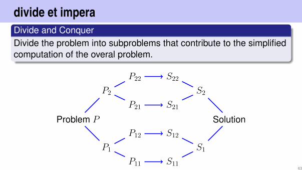
divide et imperaDivide and ConquerDivide the problem into subproblems that contribute to the simplifiedcomputation of the overal problem.
Solution
S2
S22
S21
S1
S12
S11
Problem P
P1
P11
P12
P2
P21
P22
63

Divide and Conquer!Search b = 23.
101
202
223
244
285
326
357
388
419
4210
b < 28
101
202
223
244
285
326
357
388
419
4210
b > 20
223
244
285
101
202
326
357
388
419
4210
b > 22
244
101
202
223
285
326
357
388
419
4210
b < 24
244
101
223
202
285
326
357
388
419
4210
erfolglos
64

Binary Search Algorithm BSearch(A[l..r], b)
Input: Sorted array A of n keys. Key b. Bounds 1 ≤ l ≤ r ≤ n or l > rbeliebig.
Output: Index of the found element. 0, if not found.m← b(l + r)/2cif l > r then // Unsuccessful search
return NotFoundelse if b = A[m] then// found
return melse if b < A[m] then// element to the left
return BSearch(A[l..m− 1], b)else // b > A[m]: element to the right
return BSearch(A[m+ 1..r], b)
65

Analysis (worst case)Recurrence (n = 2k)
T (n) =
d falls n = 1,T (n/2) + c falls n > 1.
Compute: 2
T (n) = T(n
2
)+ c = T
(n4
)+ 2c = ...
= T( n
2i
)+ i · c
= T(nn
)+ log2 n · c = d+ c · log2 n ∈ Θ(log n)
2Try to find a closed form of T by applying the recurrence repeatedly (starting with T (n)).66

Analysis (worst case)
T (n) =
d if n = 1,T (n/2) + c if n > 1.
Guess : T (n) = d+ c · log2 n
Proof by induction:
Base clause: T (1) = d.Hypothesis: T (n/2) = d+ c · log2 n/2
Step: (n/2→ n)
T (n) = T (n/2) + c = d+ c · (log2 n− 1) + c = d+ c log2 n.
67

Result
TheoremThe binary sorted search algorithm requires Θ(log n) fundamentaloperations.
68

Iterative Binary Search Algorithm
Input: Sorted array A of n keys. Key b.Output: Index of the found element. 0, if unsuccessful.l← 1; r ← nwhile l ≤ r do
m← b(l + r)/2cif A[m] = b then
return melse if A[m] < b then
l← m+ 1else
r ← m− 1
return NotFound ;
69

4. Sorting
Simple Sorting, Quicksort, Mergesort
70

Problem
Input: An array A = (A[1], ..., A[n]) with length n.
Output: a permutation A′ of A, that is sorted: A′[i] ≤ A′[j] for all1 ≤ i ≤ j ≤ n.
71

Selection Sort
5 6 2 8 4 1 (i = 1)
1 6 2 8 4 5 (i = 2)
1 2 6 8 4 5 (i = 3)
1 2 4 8 6 5 (i = 4)
1 2 4 5 6 8 (i = 5)
1 2 4 5 6 8 (i = 6)
1 2 4 5 6 8
Selection of the smallestelement by search in theunsorted part A[i..n] ofthe array.
Swap the smallestelement with the firstelement of the unsortedpart.
Unsorted part decreasesin size by one element(i→ i+ 1). Repeat untilall is sorted. (i = n)
72

Algorithm: Selection Sort
Input: Array A = (A[1], . . . , A[n]), n ≥ 0.Output: Sorted Array Afor i← 1 to n− 1 do
p← ifor j ← i+ 1 to n do
if A[j] < A[p] thenp← j;
swap(A[i], A[p])
73

Analysis
Number comparisons in worst case: Θ(n2).
Number swaps in the worst case: n− 1 = Θ(n)
74

4.1 Mergesort
[Ottman/Widmayer, Kap. 2.4, Cormen et al, Kap. 2.3],
75

Mergesort
Divide and Conquer!
Assumption: two halves of the array A are already sorted.Minimum of A can be evaluated with two comparisons.Iteratively: merge the two presorted halves of A in O(n).
76
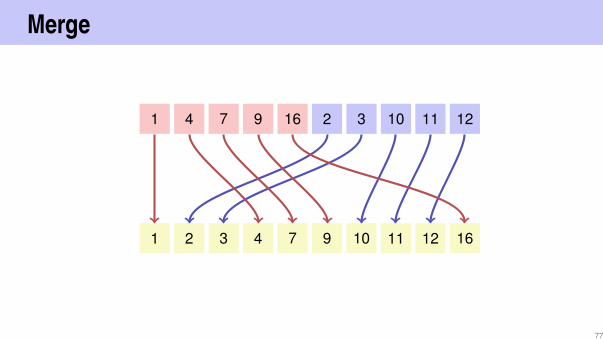
Merge
1 4 7 9 16 2 3 10 11 12
1 2 3 4 7 9 10 11 12 16
77

Algorithm Merge(A, l,m, r)
Input: Array A with length n, indexes 1 ≤ l ≤ m ≤ r ≤ n.A[l, . . . ,m], A[m+ 1, . . . , r] sorted
Output: A[l, . . . , r] sorted1 B ← new Array(r − l + 1)2 i← l; j ← m+ 1; k ← 13 while i ≤ m and j ≤ r do4 if A[i] ≤ A[j] then B[k]← A[i]; i← i+ 15 else B[k]← A[j]; j ← j + 16 k ← k + 1;
7 while i ≤ m do B[k]← A[i]; i← i+ 1; k ← k + 18 while j ≤ r do B[k]← A[j]; j ← j + 1; k ← k + 19 for k ← l to r do A[k]← B[k − l + 1]
78

Mergesort
5 2 6 1 8 4 3 9Split
5 2 6 1 8 4 3 9Split
5 2 6 1 8 4 3 9Split
5 2 6 1 8 4 3 9Merge
2 5 1 6 4 8 3 9Merge
1 2 5 6 3 4 8 9Merge
1 2 3 4 5 6 8 9
79

Algorithm (recursive 2-way) Mergesort(A, l, r)
Input: Array A with length n. 1 ≤ l ≤ r ≤ nOutput: Array A[l, . . . , r] sorted.if l < r then
m← b(l + r)/2c // middle positionMergesort(A, l,m) // sort lower halfMergesort(A,m+ 1, r) // sort higher halfMerge(A, l,m, r) // Merge subsequences
80

Analysis
Recursion equation for the number of comparisons and keymovements:
T (n) = T (⌈n
2
⌉) + T (
⌊n2
⌋) + Θ(n) ∈ Θ(n log n)
81

Derivation for n = 2k
Let n = 2k, k > 0. Recurrence
T (n) =
d if n = 1
2T (n/2) + cn if n > 1
Apply recursivelyT (n) = 2T (n/2) + cn = 2(2T (n/4) + cn/2) + cn
= 2(2(T (n/8) + cn/4) + cn/2) + cn = ...
= 2(2(...(2(2T (n/2k) + cn/2k−1)...) + cn/22) + cn/21) + cn
= 2kT (1) + 2k−1cn/2k−1 + 2k−2cn/2k−2 + ...+ 2k−kcn/2k−k︸ ︷︷ ︸kterms
= nd+ cnk = nd+ cn log2 n ∈ Θ(n log n).
82

4.2 Quicksort
[Ottman/Widmayer, Kap. 2.2, Cormen et al, Kap. 7]
83

Quicksort
? What is the disadvantage of Mergesort?
! Requires additional Θ(n) storage for merging.
? How could we reduce the merge costs?
! Make sure that the left part contains only smaller elements thanthe right part.
? How?! Pivot and Partition!
84

Use a pivot
1 Choose a (an arbitrary) pivot p2 Partition A in two parts, one part L with the elements withA[i] ≤ p and another part R with A[i] > p
3 Quicksort: Recursion on parts L and R
p > ≤ ≤ > > ≤ ≤ > ≤p >≤ ≤ > >≤ ≤ >≤p p≤
r1 n
85

Algorithm Partition(A[l..r], p)
Input: Array A, that contains the pivot p in the interval [l, r] at least once.Output: Array A partitioned in [l..r] around p. Returns position of p.while l ≤ r do
while A[l] < p dol← l + 1
while A[r] > p dor ← r − 1
swap(A[l], A[r])if A[l] = A[r] then
l← l + 1
return l-1
86

Algorithm Quicksort(A[l, . . . , r]
Input: Array A with length n. 1 ≤ l ≤ r ≤ n.Output: Array A, sorted between l and r.if l < r then
Choose pivot p ∈ A[l, . . . , r]k ← Partition(A[l, . . . , r], p)Quicksort(A[l, . . . , k − 1])Quicksort(A[k + 1, . . . , r])
87

Choice of the pivot.
The minimum is a bad pivot: worst case Θ(n2)
p1 p2 p3 p4 p5
A good pivot has a linear number of elements on both sides.
p
≥ ε · n ≥ ε · n
88

Choice of the Pivot?Randomness to our rescue (Tony Hoare, 1961). In each stepchoose a random pivot.
14
14
12
schlecht schlechtgute Pivots
Probability for a good pivot in one trial: 12 =: ρ.
Probability for a good pivot after k trials: (1− ρ)k−1 · ρ.
Expected number of trials3: 1/ρ = 23Expected value of the geometric distribution:
89

Quicksort (arbitrary pivot)
2 4 5 6 8 3 7 9 1
2 1 3 6 8 5 7 9 4
1 2 3 4 5 8 7 9 6
1 2 3 4 5 6 7 9 8
1 2 3 4 5 6 7 8 9
1 2 3 4 5 6 7 8 9
90

Analysis: number comparisons
Worst case. Pivot = min or max; number comparisons:
T (n) = T (n− 1) + c · n, T (1) = 0 ⇒ T (n) ∈ Θ(n2)
91

Analysis (randomized quicksort)
TheoremOn average randomized quicksort requires O(n · log n) comparisons.
(without proof.)
92

Practical Considerations.
Practically the pivot is often the median of three elements. Forexample: Median3(A[l], A[r], A[bl + r/2c]).
93

5. From Java to Python
First Python Program, Transfer Java→ Python, Dynamic DataStructures in Python
94
Learning Objectives
see a new programming language (Python) and learn how totransfer from one programming language to anotherlearn the most important differences between Java and Python,both from a syntactical and semantical point of viewlearn about the basic data types of Python (list, set, dict, tuple)and operations leveraging the use of such data typesget used to the new programming language and environment(Python) by re-implementing known algorithms
95

First Java Program
public class Hello public static void main (String[] args)
System.out.print("Hello World!");
96

First Python Program
print("Hello World!")
97

Comments
Comments are preceded by a #
# prints ’Hello World!’ to the consoleprint("Hello World!")
98

Formatting Matters: Statements
Whitespace is relevantEach line represents a statementSo, exactly one Statement per lineComments start with #
Example program with two statements:# two print−statementsprint("Hurray, finally ...")print("... no Semicolons!")
99

Formatting Matters: Blocks
Blocks must be indented.All indented statements are part of a block. The block ends assoon as the indentation ends.Start of a Block is marked by a colon “:”
# in Pythonwhile i > 0:
x = x + 1 / ii = i − 1
print(x)
// in Javawhile (i > 0)
x = x + 1.0 / i;i = i − 1;
System.out.print(x)
100

Literals: Numbers
integer: 42, −5, 0x1b, 0o33, 7729684762313578932578932Arbitrary precise integer numbersfloat: −0.1, 34.567e−4Like double in Java, but precision depends on platform (CPU/operating system)complex: 2 + 3j, (0.21 - 1.2j)Complex numbers in the form a+bj. Optional round parentheses.
101

Literals: Booleans
TrueFalse
102

Literals: Strings
’a single quoted string\nand a second line’"a doube quoted string\nand a second line"Multi-line strings (tripple double quotes):
"""a multiline stringand a second line"""
103

Literals: Sequences
arrays: There are no primitive arrays in Pythonlists: [ 17, True, "abc"] , []Mutable ordered sequence of 0 or more Values of arbitrary types.tuples: (17, True, "abc") , (42, )Immutable ordered sequence of 1 or more Values of arbitrarytypes.
104

Literals: Collections
dicts: "a": 42, "b": 27, False: 0 , Mutable Key-Value store. Keys and values may have arbitrarytypes.sets: 17, True, "abc" , 42Mutable unordered sequence of 0 or more Values of arbitrarytypes. No duplicates.
105

Variables
Variables are automatically created upon the first assignmentThe type of a variable is not checked upon assignment. That is,values of different types can be assigned to a variable over time.Assignment of values with the assignment operator: =Assignment to multiple variables with tuples
a = "Ein Text"print(a) # prints: Ein Texta = 42print(a) # prints: 42
x, y = 4, 5print(x) # prints: 4print(y) # prints: 5
106

Variables
Variables must always be assigned first before it’s possible to readtheir value
Assume b never got a value assigned:a = b
Results in the following error
NameError: name ’b’ is not defined
107

Numeric and Boolean Operators
Numeric operators as in Java: +, −, ∗, /, %, ∗∗, //Caution: “ / ” always results in a floating-point number∗∗: Power function, a∗∗b = ab.//: Integer division, 5//2 results in 2.5.Comparison operators as in Java: ==, >=, <=, >, <, !=Logical Operators: and, or, notMembership Operator: “ in ” Determines if a value is in a list, setor string.Identity Operator: “ is ” Checks if two variables point to the sameobject.
108

Input/Output
Reading of inputs using input()A prompt can be provided.Output using print(...)print accepts one or more arguments and prints them separatedwith a space
name = input("What is your name: ")print("Hello", name)
109

Input/Output
Input is always read as stringTo read a number, the input must be converted to a number firstNo implicit conversion happensExplicit conversion using:int(), float(), complex(), list(), ...
i = int(input("Enter a number: "))print("The", i,"th power of two is", 2∗∗i)
110

Conditions
No parentheses required around the testelif to test another caseMind the indentation!
a = int(input("Enter a number: "))if a == 42:
print("Naturally, the answer")elif a == 28:
print("A perfect number, good choice")else:
print(a, "is just some boring number")
111

While-Loops
The well-known Collaz-Folgea = int(input("Enter a number: "))while a != 1:
if a % 2 == 0:a = a // 2
else:a = a ∗ 3 + 1
print(a, end=’ ’)
112

For-Loops
For-Loops work differently than in JavaIterates over the elements of the given set
some_list = [14, ’lala’, 22, True, 6]total = 0;for item in some_list:
if type(item) == int:total += item
print("Total of the numbers is", total)
113

For-Loops over a value range
The function range(start, end, step) creates a list of values,starting with start until end - exclusive. Stepsize is step.Step size is 1 if the third argument is omitted.
# the following loop prints "1 2 3 4"for i in range(1,5):
print(i, end=’ ’)
# the following loop prints "10 8 6 4 2"for i in range(10, 0, −2):
print(i, end=’ ’)
114

MethodsThe Cookie Calculator revisited
def readInt(prompt, atleast = 1):"""Prompt for a number greater 0 (or min, if specified)"""number = 0;while number < atleast:
number = int(input(prompt))if (number < atleast):
print("Too small, pick a number larger than", atleast)return number
kids = readInt("Kids: ")cookies = readInt("Cookies: ", atleast=kids)print("Each Kid gets", cookies // kids, "cookies.")print("Papa gets", cookies % kids, "cookies.")
115

Lists: Basic OperationsElement-Access (0-based): a[2] points to the third element.Negative indices count from the last element!
a = [ 3, 7, 4]print(a[−1]) # prints ’4’
Add value to the tail: a.append(12)Test if an element is in a collection:
if 12 in a:print(’12 is in the list, we just added it before’)
Anzahl Elemente in einer Collection: len(a)116

Lists: Slicing
Slicing: address partition: a[start:end]a and/or b are positive or negative indices.end is not inclusive
a = [ 1, 2, 3, 4, 5, 6, 7, 8, 9]print(a[2:4]) # [3, 4]print(a[3:−3]) # [4, 5, 6]print(a[−3:−1]) # [7, 8]print(a[5:]) # [6, 7, 8, 9]print(a[:3]) # [1, 2, 3]
117

Dictionaries
Dictionaries are very important primitive data structures in Python
Easy and efficient possibility to name and group several fields ofdataBuild hierarchical data structures by nestingAccessing elements using [] Operator
record = ’Firstname’: ’Hermann’, ’Lastname’:’Lehner’,’Salary’: 420000, ’Mac User’: True
record[’Salary’] = 450000if record[’Mac User’]:
print(’... one more thing!’)
118

Dynamic Data Structures with Dictstree =
’key’: 8,’left’ :
’key’: 4, ’left’ : None, ’right’: None,’right’:
’key’: 13,’left’ :
’key’: 10, ’left’ : None, ’right’: None,’right’:
’key’: 19, ’left’ : None, ’right’: None
8
4 13
10 19
119

Dynamic Data Structures with Dicts
Working with Dicts (Examples)
l = tree[’left’] # assign left subtree to variable ll[’key’] = 6 # changes key from 4 to 6
if l[’left’] is None: # proper way to test against Noneprint("There is no left child here...")
else:print("Value of left subtree is", l[’left’][’key’]
120

Dynamic Data Structures with Classesclass Node:
def __init__(self, k, l=None, r=None):self.key, self.left, self.right = k, l, r
# create the tree depicted on the rightrightSubtree = Node(13, l=Node(10), r=Node(19))tree = Node(8, l=Node(4), r=rightSubtree)
# an example queryprint(tree.right.right.key) # prints: 19
8
4 13
10 19
121

Modules
Python has a vast amount of libraries in form of modules that can beimported.
Importaing a whole module:
import mathx = math.sqrt(4)
from math import ∗x = sqrt(4)
Importaing parts of a module:
from datetime import datet = date.today()
122

6. Advanced Python Concepts
Built-in Functions, Conditional Expressions, List and DictComprehension, File IO, Exception-Handling
123

Built-In Functions: Enumerate with IndicesSometimes, one wants to iterate through a list, including the index ofeach element. This works with enumerate( ... )
data = [ ’Spam’, ’Eggs’, ’Ham’ ]
for index, value in enumerate(data):print(index, ":", value)
Output:0 : Spam1 : Eggs2 : Ham
124

Built-In Functions: Combining lists
There is a simple possibility to combine lists element-wise (like azipper!): zip( ... )
places = [ ’Zurich’, ’Basel’, ’Bern’]plz = [ 8000, 4000, 3000, ]
list(zip(places, plz)# [(’Zurich’, 8000), (’Basel’, 4000), (’Bern’, 3000)]
dict(zip(places, plz)# ’Zurich’: 8000, ’Basel’: 4000, ’Bern’: 3000
125
Conditional Expressions
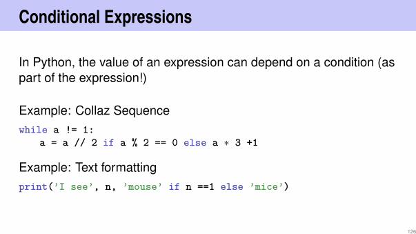
In Python, the value of an expression can depend on a condition (aspart of the expression!)
Example: Collaz Sequencewhile a != 1:
a = a // 2 if a % 2 == 0 else a ∗ 3 +1
Example: Text formattingprint(’I see’, n, ’mouse’ if n ==1 else ’mice’)
126

List Comprehension
Python provides a convenient way of creating lists declarativelySimilar technique to ‘map’ and ‘filter’ in functional languages
Example: Read-in a sequence of numbersline = input(’Enter some numbers: ’)s_list = line.split()n_list = [ int(x) for x in s_list ]
The same combined in one expressionn_list = [ int(x) for x in input(’Enter some numbers: ’).split() ]
127

List Comprehension
Example: Eliminate whitespace in front and at the backline = [ ’ some eggs ’, ’ slice of ham ’, ’ a lot of spam ’ ]cleaned = [ item.strip() for item in line ]
# cleaned == [ ’some eggs’, ’slice of ham’, ’a lot of spam’ ]
128

Dict ComprehensionLike with lists, but with key/value pairs
Example: extract data from a dictdata =
’Spam’ : ’Amount’ : 12, ’Price’: 0.45 ,’Eggs’ : ’Price’: 0.8 ,’Ham’ : ’Amount’: 5, ’Price’: 1.20
total_prices = item : record[’Amount’] ∗ record[’Price’]for item, record in data.items()if ’Amount’ in record
# total_prices == ’Spam’: 5.4, ’Ham’: 6.0129

File IO
Files can be opened with the command openTo automatically close files afterwards, this must happen in a withblock
Example: Read CSV fileimport csv
with open(’times.csv’, mode=’r’) as csv_file:csv_lines = csv.reader(csv_file)for line in csv_lines:
# do something for each record
Writing works similarly. See Python documentation.130

Exception Handling
Given the following code:
x = int(input(’A number please: ’))
If no number is entered, the program crashes:
Traceback (most recent call last):File "main.py", line 1, in <module>
x = int(input(’A number please: ’))ValueError: invalid literal for int() with base 10: ’a’
We can catch this error and react accordingly.
131

Exception Handling
try:x = int(input(’A number please: ’))
except ValueError:print(’Oh boy, that was no number...’)x = 0
print(’x:’, x)
Output, if spam is entered instead of a number:
Oh boy, that was no number...x: 0
132

7. Java Input/Output
User Input/Console Output, File Input and Output (I/O)
133

User Input (half the truth)
e.g. reading a number: int i = In.readInt();Our class In provides various such methods.Some of those methods have to deal with wrong inputs: Whathappens with readInt() for the following input?
"spam"
134

User Input (half the truth)
public class Main public static void main(String[] args)
Out.print("Number: ");int i = In.readInt ();Out.print("Your number: " + i);
It seems not much happens!
Number: spamYour number: 0
135

User Input (the whole truth)e.g. reading a number using the class Scanner
import java. util .Scanner;public class Main
public static void main(String[] args) Out.print("Number: ");Scanner input = new Scanner(System.in);int i = input.nextInt();Out.print("Your number: " + i);
What happens for the following input?
"spam"136

User Input (the whole truth)
Number: spamException in thread "main" java. util .InputMismatchException
at java .base/java. util .Scanner.throwFor(Scanner.java:939)at java .base/java. util .Scanner.next(Scanner.java:1594)at java .base/java. util .Scanner.nextInt(Scanner.java:2258)at java .base/java. util .Scanner.nextInt(Scanner.java:2212)at Main.main(Main.java:7)at TestRunner.main(TestRunner.java:330)
Oh, we come back to this in the next chapter...
137

Console Output
Until now, you knew: Out.print("Hi") oderOut.println("Hi")Without our Out class:
System.out.print("The answer is: " );System.out.println(42);System.out.println("What was the question?!");
This leads to the following output:
The answer is: 42What was the question?!
138

So: User Input/Console Output
Reading of input via the input stream System.inWriting of output via output stream System.out
139

Reading/Writing Files (line by line)
Files can be read byte by byte using the classjava.io.FileReaderTo read entire lines, we use in addition ajava.io.BufferedReaderFiles can be written byte by byte using the classjava.io.FileWriterTo read entire lines, we use in addition ajava.io.BufferedWriter
140

Reading Files (line by line)
import java.io.FileReader;import java.io.BufferedReader;
public class Main public static void main(String[] args)
FileReader fr = new FileReader("gedicht.txt");BufferedReader bufr = new BufferedReader(fr);String line;while ((line = bufr.readLine()) != null)
System.out.println(line);
141

Reading Files (line by line)
We get the following compilation error:./Main.java:6: error: unreported exception FileNotFoundException;
must be caught or declared to be thrownFileReader fr = new FileReader("gedicht.txt");
^./Main.java:9: error: unreported exception IOException; must be
caught or declared to be thrownwhile ((line = bufr.readLine()) != null)
^2 errors
It seems we need to understand more about the topic “Exceptions”
142

... therefore ...
143

8. Errors and Exceptions
Errors, runtime-exceptions, checked-exceptions, exception handling,special case: resources
144

Errors and Exceptions in Java
Exceptions are bad, or not?
Errors and exceptions interrupt thenormal execution of the program abruptlyand represent an unplanned event.
Java allows to catch such events and deal with it (as opposed to crashing theentire program)
Unhandled errors and exceptions are passed up through the call stack.
145

Errors
This glass is broken for good
Errors happen in the virtual machine ofJava and are not repairable.
Examples
No more memory available
Too high call stack (→ recursion)
Missing libraries
Bug in the virtual machine
Hardware error
146

Exceptions
Exceptions are triggered by the virtual machine or the program itselfand can typically be handled in order to re-establish the normalsituation
Clean-up and pour in a new glass
Examples
De-reference null
Division by zero
Read/write errors (on files)
Errors in business logic
147

Exception Types
Runtime Exceptions
Can happen anywhere
Can be handled
Cause: bug in the code
Checked Exceptions
Must be declared
Must be handled
Cause: Unlikely but not impossibleevent
148

Example of a Runtime Exception
1 import java. util .Scanner;2 class ReadTest 3 public static void main(String[] args)4 int i = readInt("Number");5 6 private static int readInt(String prompt)7 System.out.print(prompt + ": ");8 Scanner input = new Scanner(System.in);9 return input.nextInt ();
10 11
Input: Number: asdf149

Unhandled Errors and Exceptions
The program crashes and leaves behind a stack trace. In there, wecan see the where the program got interrupted.
Exception in thread "main" java. util .InputMismatchException[...]
at java . util .Scanner.nextInt(Scanner.java:2076)at ReadTest.readInt(ReadTest.java:9)at ReadTest.main(ReadTest.java:4)
⇒ Forensic investigation based on this information.
150

Exception gets Propagated through Call Stack
Java VM Runtime
ReadTest.main
ReadTest.main();
ReadTest.readInt
int i = readInt("Number");
Scanner.nextInt
return input.nextInt();
88
88
88
=
151

Unstanding Stack Traces
Output:
Exception in thread "main" java.util.InputMismatchExceptionat java . util .Scanner.throwFor(Scanner.java:864)at java . util .Scanner.next(Scanner.java:1485)at java . util .Scanner.nextInt(Scanner.java:2117)at java . util .Scanner.nextInt(Scanner.java:2076)at ReadTest.readInt(ReadTest.java:9)at ReadTest.main(ReadTest.java:4)
An unsuited input ...
... in method readInt on line 9 ...
... called by method main on line 4. 152

Unstanding Stack Traces
1 import java. util .Scanner;2 class ReadTest 3 public static void main(String[] args)4 int i = readInt("Number");5 6 private static int readInt(String prompt)7 System.out.print(prompt + ": ");8 Scanner input = new Scanner(System.in);9 return input.nextInt ();
10 11
at ReadTest.readInt(ReadTest.java:9)at ReadTest.main(ReadTest.java:4)at ReadTest.readInt(ReadTest.java:9)at ReadTest.main(ReadTest.java:4)
153

Runtime Exception: Bug in the Code?!
Where is the bug?
private static int readInt(String prompt)System.out.print(prompt + ": ");Scanner input = new Scanner(System.in);return input.nextInt();
Not guaranteed that the next input is an int
⇒ The scanner class provides a test for this154

Runtime Exception: Bug Fix!
Check first!
private static int readInt(String prompt)System.out.print(prompt + ": ");Scanner input = new Scanner(System.in);if (input.hasNextInt())
return input.nextInt (); else
return 0; // or do something else ...?!
155

First Finding: often no Exceptional Situation
Often, those “exceptional” cases aren’t that unusual, but prettyforeseeable. In those cases no exceptions should be used!
Kids are tipping over cups. You get used to it.
Examples
Wrong credentials when logging in
Empty required fields in forms
Unavailable internet resources
Timeouts
156

Second Finding: Avoid Exceptions
Problem solved.
Instead of letting a runtime exception happen, ac-tively prevent such a situation to arise.
Examples
Check user inputs early
Use optional types
Predict timeout situations
Plan B for unavailable resources
157

Exception Types
Runtime Exceptions
Can happen anywhere
Can be handled
Cause: bug in the code
Checked Exceptions
Must be declared
Must be handled
Cause: Unlikely but not impossibleevent
158

Example of a Checked Exception
private static String[] readFile(String filename)FileReader fr = new FileReader(filename);BufferedReader bufr = new BufferedReader(fr);...line = bufr.readLine();...
Compiler Error:./Root/Main.java:9: error: unreported exception FileNotFoundException; must be caught or declared to be thrown
FileReader fr = new FileReader(filename);^
./Root/Main.java:11: error: unreported exception IOException; must be caught or declared to be thrownString line = bufr.readLine();
^2 errors
159

Quick Look into Javadoc
160
Why use Checked Exceptions?
The following situations justify checked exception:
Fault is unprobable but not impossibe – and can be fixed by takingsuitable measures at runtime.
The caller of a method with a declared checked exception is forcedto deal with it – catch it or pass it up.
161

Handling Exceptions
private static String[] readFile(String filename)try
FileReader fr = new FileReader(filename);BufferedReader bufr = new BufferedReader(fr);...line = bufr.readLine();...
catch (IOException e)// do some recovery handling
finally // close resources
Protectedscope
Measures to re-establis thenormal situation
Gets executed in any case, atthe end, always!
162

Handling Exceptions: Stop Propagation!
Java VM Runtime
ReadTest.main
ReadTest.main();
ReadTest.readFile
lines = readFile("dataset.csv");
BufferedReader.readLine
line = bufr.readLine();
88
4Exception caught!
163

Finally: Closing Resources
In Java, resources must be closed after use at all costs. Otherwise,memory won’t get freed.
Resources:
FilesData streamsUI elements. . .
164

Try-With-Resources Statement
Specific syntax to close resources automatically:private static String[] readFile(String filename)
try ( FileReader fr = new FileReader(filename);BufferedReader bufr = new BufferedReader(fr))
...line = bufr.readLine();...
catch (IOException e)// do some recovery handling
Resources getopened here
Resources get closed automatically here
165

9. Hashing
Hash Tables, Pre-Hashing, Hashing, Resolving Collisions usingChaining, Simple Uniform Hashing, Popular Hash Functions,Table-Doubling, Open Addressing: Probing [Ottman/Widmayer, Kap.4.1-4.3.2, 4.3.4, Cormen et al, Kap. 11-11.4]
166

Motivating Example
Gloal: Efficient management of a table of all n ETH-students of
Possible Requirement: fast access (insertion, removal, find) of adataset by name
167
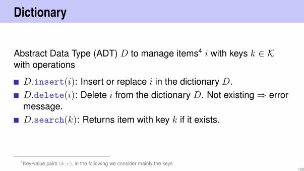
Dictionary
Abstract Data Type (ADT) D to manage items4 i with keys k ∈ Kwith operations
D.insert(i): Insert or replace i in the dictionary D.D.delete(i): Delete i from the dictionary D. Not existing⇒ errormessage.D.search(k): Returns item with key k if it exists.
4Key-value pairs (k, v), in the following we consider mainly the keys168

Dictionaries in Pythonfruits =
"banana": 2.95, "kiwi": 0.70,"pear": 4.20, "apple": 3.95
fruits["melon"] = 3.95fruits["banana"] = 1.90print("banana", fruits["banana"])print("melon in fruits", "melon" infruits)print("onion in fruits", "onion" in fruits)del fruits["strawberry"]for name,price in fruits.items():
print(name,"−>",price)
dictionary
insertupdate
find
removeiterate
169

Dictionaries in Java
Map<String,Double> fruits =new HashMap<String,Double>();
fruits.put("banana", 2.95);fruits.put("kiwi", 0.70);fruits.put("strawberry", 9.95);fruits.put("pear", 4.20);fruits.put("apple", 3.95);fruits.put("banana", 2.90);Out.println("banana " + fruits.get("banana"));fruits.remove("banana");for (String s: fruits.keySet())
Out.println(s+" " + fruits.get(s));
dictionary
insert
updatefind
removeiterate
170

Motivation / UsePerhaps the most popular data structure.
Supported in many programming languages (C++, Java, Python,Ruby, Javascript, C# ...)Obvious use
Databases, SpreadsheetsSymbol tables in compilers and interpreters
Less obvious
Substrin Search (Google, grep)String commonalities (Document distance, DNA)File SynchronisationCryptography: File-transfer and identification
171

1. Idea: Direct Access Table (Array)
Index Item0 -1 -2 -3 [3,value(3)]4 -5 -...
...k [k,value(k)]...
...
Problems1 Keys must be non-negative
integers2 Large key-range⇒ large array
172

Solution to the first problem: Pre-hashing
Prehashing: Map keys to positive integers using a functionph : K → N
Theoretically always possible because each key is stored as abit-sequence in the computerTheoretically also: x = y ⇔ ph(x) = ph(y)
Practically: APIs offer functions for pre-hashing. (Java:object.hashCode(), C++: std::hash<>, Python:hash(object))APIs map the key from the key set to an integer with a restrictedsize.5
5Therefore the implication ph(x) = ph(y)⇒ x = y does not hold any more for all x,y.173

Prehashing Example : String
Mapping Name s = s1s2 . . . sls to key
ph(s) =
(ls∑i=1
sls−i+1 · bi)
mod 2w
b so that different names map to different keys as far as possible.
b Word-size of the system (e.g. 32 or 64)
Example (Java) with b = 31, w = 32. Ascii-Values si.Anna 7→ 2045632Jacqueline 7→ 2042089953442505 mod 232 = 507919049
174

Implementation Prehashing (String) in Java
phb,m(s) =
(l−1∑i=0
sl−i+1 · bi)
mod m
With b = 31 and m = 232 we get in Java6
int prehash(String s)int h = 0;for (int k = 0; k < s.length(); ++k)
h = h ∗ b + s.charAt(k);return h;
6Try to understand why this works
175

Losung zum zweiten Problem: HashingReduce the universe. Map (hash-function) h : K → 0, ...,m− 1(m ≈ n = number entries of the table)
Collision: h(ki) = h(kj).176

Nomenclature
Hash funtion h: Mapping from the set of keys K to the index set0, 1, . . . ,m− 1 of an array (hash table).
h : K → 0, 1, . . . ,m− 1.
Normally |K| m. There are k1, k2 ∈ K with h(k1) = h(k2)(collision).
A hash function should map the set of keys as uniformly as possibleto the hash table.
177

Resolving Collisions: ChainingExample m = 7, K = 0, . . . , 500, h(k) = k mod m.Keys 12 , 55 , 5 , 15 , 2 , 19 , 43
Direct Chaining of the Colliding entries
15
43
2 12
5
19
55
hash table
Colliding entries
0 1 2 3 4 5 6
178

Algorithm for Hashing with Chaining
insert(i) Check if key k of item i is in list at position h(k). If no,then append i to the end of the list. Otherwise replace element byi.find(k) Check if key k is in list at position h(k). If yes, return thedata associated to key k, otherwise return empty element null.delete(k) Search the list at position h(k) for k. If successful,remove the list element.
179

Worst-case Analysis
Worst-case: all keys are mapped to the same index.
⇒ Θ(n) per operation in the worst case.
180

Simple Uniform Hashing
Strong Assumptions: Each key will be mapped to one of the mavailable slots
with equal probability (Uniformity)and independent of where other keys are hashed(Independence).
181
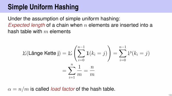
Simple Uniform HashingUnder the assumption of simple uniform hashing:Expected length of a chain when n elements are inserted into ahash table with m elements
E(Länge Kette j) = E
(n−1∑i=0
1(ki = j)
)=
n−1∑i=0
P(ki = j)
=n∑i=1
1
m=n
m
α = n/m is called load factor of the hash table.182

Simple Uniform Hashing
TheoremLet a hash table with chaining be filled with load-factor α = n
m < 1.Under the assumption of simple uniform hashing, the next operationhas expected costs of ≤ 1 + α.
Consequence: if the number slots m of the hash table is always atleast proportional to the number of elements n of the hash table,n ∈ O(m)⇒ Expected Running time of Insertion, Search andDeletion is O(1).
183

Advantages and Disadvantages of Chaining
Advantages
Possible to overcommit: α > 1 allowedEasy to remove keys.
Disadvantages
Memory consumption of the chains-
184

An Example of a popular Hash Function
Division methodh(k) = k mod m
Ideal: m prime, not too close to powers of 2 or 10
But often: m = 2k − 1 (k ∈ N)
Other method: multiplication method (cf. Cormen et al, Kap. 11.3).
185

Table size increase
We do not know beforehand how large n will beRequire m = Θ(n) at all times.
Table size needs to be adapted. Hash-Function changes⇒rehashing
Allocate array A′ with size m′ > m
Insert each entry of A into A′ (with re-hashing the keys)Set A← A′.Costs O(n+m+m′).
How to choose m′?186

Table size increase
1.Idea n = m⇒ m′ ← m+ 1Increase for each insertion: Costs Θ(1 + 2 + 3 + · · ·+ n) = Θ(n2)
2.Idea n = m⇒ m′ ← 2m Increase only ifm = 2i:Θ(1 + 2 + 4 + 8 + · · ·+ n) = Θ(n)Few insertions cost linear time but on average we have Θ(1)
Jede Operation vom Hashing mit Verketten hat erwartet amortisierteKosten Θ(1).
(⇒ Amortized Analysis)
187

Amortisierte AnalyseGeneral procedure for dynamic arrays (e.g. Java: ArrayList,Python: List)
The data structure provides, besides the data array, two numbers:size of the array (capacity m) and the number of used entries (sizen)Double the size and copy entries when the list is fulln = m ⇒ m← 2n. Kosten Θ(m).Runtime costs for n = 2k insertion operations:Θ(1 + 2 + 4 + 8 + · · ·+ 2k) = Θ(2k+1 − 1) = Θ(n).
Costs per operation averaged over all operations = amortized costs= Θ(1) per insertion operation
188

Open Addressing7
Store the colliding entries directly in the hash table using a probingfunction s : K × 0, 1, . . . ,m− 1 → 0, 1, . . . ,m− 1Key table position along a probing sequence
S(k) := (s(k, 0), s(k, 1), . . . , s(k,m− 1)) mod m
Probing sequence must for each k ∈ K be a permutation of0, 1, . . . ,m− 1
7Notational clarification: this method uses open addressing(meaning that the positions in the hashtable are not fixed) butit is a closed hashing procedure (because the entries stay in the hashtable)
189

Algorithms for open addressing
insert(i) Search for kes k of i in the table according to S(k). If kis not present, insert k at the first free position in the probingsequence. Otherwise error message.find(k) Traverse table entries according to S(k). If k is found,return data associated to k. Otherwise return an empty elementnull.delete(k) Search k in the table according to S(k). If k is found,replace it with a special key removed.
190

Linear Probing
s(k, j) = h(k) + j ⇒ S(k) = (h(k), h(k) + 1, . . . , h(k) +m− 1)mod m
Example m = 7, K = 0, . . . , 500, h(k) = k mod m.Key 12 , 55 , 5 , 15 , 2 , 19
0 1 2 3 4 5 6
12 555 15 2 19
191

Discussion
Example α = 0.95
The unsuccessful search consideres 200 table entries on average!(here without derivation).
? Disadvantage of the method?
! Primary clustering: similar hash addresses have similar probingsequences⇒ long contiguous areas of used entries.
192

Quadratic Probing
s(k, j) = h(k) + dj/2e2 (−1)j+1
S(k) = (h(k), h(k) + 1, h(k)− 1, h(k) + 4, h(k)− 4, . . . ) mod m
Example m = 7, K = 0, . . . , 500, h(k) = k mod m.Keys 12 , 55 , 5 , 15 , 2 , 19
0 1 2 3 4 5 6
12 55515 219
193

Discussion
Example α = 0.95
Unsuccessfuly search considers 22 entries on average (here withoutderivation)
? Problems of this method?! Secondary clustering: Synonyms k and k′ (with h(k) = h(k′))
travers the same probing sequence.
194

Double Hashing
Two hash functions h(k) and h′(k). s(k, j) = h(k) + j · h′(k).S(k) = (h(k), h(k) + h′(k), h(k) + 2h′(k), . . . , h(k) + (m− 1)h′(k)) mod m
Example:m = 7, K = 0, . . . , 500, h(k) = k mod 7, h′(k) = 1 + k mod 5.Keys 12 , 55 , 5 , 15 , 2 , 19
0 1 2 3 4 5 6
12 555 15 2 19
195

Double Hashing
Probing sequence must permute all hash addresses. Thush′(k) 6= 0 and h′(k) may not divide m, for example guaranteedwith m prime.h′ should be as independent of h as possible (to avoid secondaryclustering)
Independence largely fulfilled by h(k) = k mod m andh′(k) = 1 + k mod (m− 2) (m prime).
196

Uniform Hashing
Strong assumption: the probing sequence S(k) of a key l is equalylikely to be any of the m! permutations of 0, 1, . . . ,m− 1(Double hashing is reasonably close)
197

Analysis of Uniform Hashing with Open Addressing
TheoremLet an open-addressing hash table be filled with load-factorα = n
m < 1. Under the assumption of uniform hashing, the nextoperation has expected costs of ≤ 1
1−α .
Without Proof, cf. e.g. Cormen et al, Kap. 11.4
198

10. Repetition Binary Search Trees andHeaps
[Ottman/Widmayer, Kap. 2.3, 5.1, Cormen et al, Kap. 6, 12.1 - 12.3]
199

Dictionary implementation
Hashing: implementation of dictionaries with expected very fastaccess times.
Disadvantages of hashing: linear access time in worst case. Someoperations not supported at all:
enumerate keys in increasing ordernext smallest key to given key
200

Nomenclature
Wurzel
W
I E
K
parent
child
inner node
leaves
Order of the tree: maximum number of child nodes, here: 3Height of the tree: maximum path length root – leaf (here: 4)
201

Binary TreesA binary tree is either
a leaf, i.e. an empty tree, oran inner leaf with two trees Tl (left subtree) and Tr (right subtree)as left and right successor.
In each node v we store
a key v.key andtwo nodes v.left and v.right to the roots of the left and rightsubtree.a leaf is represented by the null-pointer
key
left right
202

Baumknoten in Java
public class SearchNode int key;SearchNode left;SearchNode right;
SearchNode(int k)key = k;left = right = null;
5
3 8
2
null null
null null null
SearchNodekey (type int)
left (type SearchNode) right (type SearchNode)
203

Baumknoten in Python
class SearchNode:def __init__(self, k, l=None, r=None):
self.key = kself.left, self.right = l, rself.flagged = False
5
3 8
2
None None
None None None
SearchNodekey
left right
204

Binary search treeA binary search tree is a binary tree that fulfils the search treeproperty:
Every node v stores a keyKeys in left subtree v.left are smaller than v.keyKeys in right subtree v.right are greater than v.key
16
7
5
2
10
9 15
18
17 30
99
205

Searching
Input: Binary search tree with root r, key kOutput: Node v with v.key = k or nullv ← rwhile v 6= null do
if k = v.key thenreturn v
else if k < v.key thenv ← v.left
elsev ← v.right
return null
8
4 13
10
9
19
Search (12)→ null
206

Insertion of a key
Insertion of the key kSearch for kIf successful search: outputerrorNo success: replace thereached leaf by a new nodewith key
8
4
5
13
10
9
19
Insert (5)
207

Remove node
Three cases possible:Node has no childrenNode has one childNode has two children
[Leaves do not count here]
8
3
5
4
13
10
9
19
208

Remove node
Node has no childrenSimple case: replace node by leaf.
8
3
5
4
13
10
9
19
remove(4)−→
8
3
5
13
10
9
19
209
Remove node
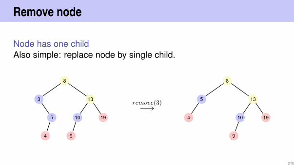
Node has one childAlso simple: replace node by single child.
8
3
5
4
13
10
9
19
remove(3)−→
8
5
4
13
10
9
19
210

Remove node
Node has two children
The following observation helps: thesmallest key in the right subtree v.right(the symmetric successor of v)
is smaller than all keys in v.rightis greater than all keys in v.leftand cannot have a left child.
Solution: replace v by its symmetric suc-cessor.
8
3
5
4
13
10
9
19
211

By symmetry...
Node has two children
Also possible: replace v by its symmetricpredecessor.
8
3
5
4
13
10
9
19
212

Algorithm SymmetricSuccessor(v)
Input: Node v of a binary search tree.Output: Symmetric successor of vw ← v.rightx← w.leftwhile x 6= null do
w ← xx← x.left
return w
213

Traversal possibilities
preorder: v, then Tleft(v), thenTright(v).8, 3, 5, 4, 13, 10, 9, 19postorder: Tleft(v), then Tright(v), thenv.4, 5, 3, 9, 10, 19, 13, 8inorder: Tleft(v), then v, then Tright(v).3, 4, 5, 8, 9, 10, 13, 19
8
3
5
4
13
10
9
19
214

Height of a tree
The height h(T ) of a tree T with root r is given by
h(r) =
0 if r = null1 + maxh(r.left), h(r.right) otherwise.
The worst case run time of the search is thus O(h(T ))
215

Analysis
Search, Insertion and Deletion of an element v from a tree Trequires O(h(T )) fundamental steps in the worst case.
216

Possible Heights
1 The maximal height hn of a tree with n inner nodes is given withh1 = 1 and hn+1 ≤ 1 + hn by hn ≥ n.
2 The minimal height hn of an (ideally balanced) tree with n innernodes fulfils n ≤
∑h−1i=0 2i = 2h − 1.
Thusdlog2(n+ 1)e ≤ h ≤ n
217

Further supported operations
Min(T ): Read-out minimal value inO(h)
ExtractMin(T ): Read-out and removeminimal value in O(h)
List(T ): Output the sorted list ofelementsJoin(T1, T2): Merge two trees withmax(T1) < min(T2) in O(n).
8
3
5
4
13
10
9
19
218

Degenerated search trees
9
5
4 8
13
10 19
Insert 9,5,13,4,8,10,19ideally balanced
4
5
8
9
10
13
19
Insert 4,5,8,9,10,13,19linear list
19
13
10
9
8
5
4
Insert 19,13,10,9,8,5,4linear list
219
[Probabilistically]
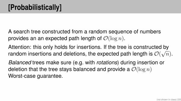
A search tree constructed from a random sequence of numbersprovides an an expected path length of O(log n).
Attention: this only holds for insertions. If the tree is constructed byrandom insertions and deletions, the expected path length is O(
√n).
Balanced trees make sure (e.g. with rotations) during insertion ordeletion that the tree stays balanced and provide a O(log n)Worst-case guarantee.
(not shown in class) 220

[Max-]Heap8
Binary tree with the following prop-erties
1 complete up to the lowestlevel
2 Gaps (if any) of the tree inthe last level to the right
3 Heap-Condition:Max-(Min-)Heap: key of achild smaller (greater) thatthat of the parent node
root
22
20
16
3 2
12
8 11
18
15
14
17
parent
child
8Heap(data structure), not: as in “heap and stack” (memory allocation)221

Heap and Array
Tree→ Array:children(i) = 2i, 2i+ 1parent(i) = bi/2c
22
1
20
2
18
3
16
4
12
5
15
6
17
7
3
8
2
9
8
10
11
11
14
12
parent
Children
22
20
16
3 2
12
8 11
18
15
14
17
[1]
[2] [3]
[4] [5] [6] [7]
[8] [9] [10] [11] [12]
Depends on the starting index9
9For array that start at 0: 2i, 2i + 1 → 2i + 1, 2i + 2, bi/2c → b(i− 1)/2c222

Height of a HeapA complete binary tree with height10 h provides
1 + 2 + 4 + 8 + ...+ 2h−1 =h−1∑i=0
2i = 2h − 1
nodes. Thus for a heap with height h:
2h−1 − 1 < n ≤ 2h − 1
⇔ 2h−1 < n+ 1 ≤ 2h
Particularly h(n) = dlog2(n+ 1)e and h(n) ∈ Θ(log n).10here: number of edges from the root to a leaf
223

Insert
Insert new element at the first freeposition. Potentially violates the heapproperty.Reestablish heap property: climbsuccessivelyWorst case number of operations:O(log n)
22
20
16
3 2
12
8 11
18
15
14
17
22
20
16
3 2
12
8 11
21
18
14 15
17
224

Remove the maximum
Replace the maximum by the lowerright elementReestablish heap property: sift downsuccessively (in the direction of thegreater child)Worst case number of operations:O(log n)
21
20
16
3 2
12
8 11
18
15
14
17
20
16
14
3 2
12
8 11
18
15 17
225

Algorithm SiftDown(A, i,m)Input: Array A with heap structure for the children of i. Last element
m.Output: Array A with heap structure for i with last element m.while 2i ≤ m do
j ← 2i; // j left childif j < m and A[j] < A[j + 1] then
j ← j + 1; // j right child with greater key
if A[i] < A[j] thenswap(A[i], A[j])i← j; // keep sinking down
elsei← m; // sift down finished
226

Sort heap
A[1, ..., n] is a Heap.While n > 1
swap(A[1], A[n])SiftDown(A, 1, n− 1);n← n− 1
7 6 4 5 1 2
swap ⇒ 2 6 4 5 1 7
siftDown ⇒ 6 5 4 2 1 7
swap ⇒ 1 5 4 2 6 7
siftDown ⇒ 5 4 2 1 6 7
swap ⇒ 1 4 2 5 6 7
siftDown ⇒ 4 1 2 5 6 7
swap ⇒ 2 1 4 5 6 7
siftDown ⇒ 2 1 4 5 6 7
swap ⇒ 1 2 4 5 6 7
227

Heap creation
Observation: Every leaf of a heap is trivially a correct heap.
Consequence: Induction from below!
228

Algorithm HeapSort(A, n)
Input: Array A with length n.Output: A sorted.// Build the heap.for i← n/2 downto 1 do
SiftDown(A, i, n);
// Now A is a heap.for i← n downto 2 do
swap(A[1], A[i])SiftDown(A, 1, i− 1)
// Now A is sorted.
229

Analysis: sorting a heap
SiftDown traverses at most log n nodes. For each node 2 keycomparisons. ⇒ sorting a heap costs in the worst case 2 log ncomparisons.
Number of memory movements of sorting a heap also O(n log n).
230

[Analysis: creating a heap]
Calls to siftDown: n/2. Thus number of comparisons andmovements: v(n) ∈ O(n log n).But mean length of the sift-down paths is much smaller:
v(n) =
blognc∑l=0
2l︸︷︷︸number heaps on level l
· (blog nc − l)︸ ︷︷ ︸height heaps on level l
=
blognc∑k=0
2blognc−k · k
≤blognc∑k=0
n
2k· k = n ·
blognc∑k=0
k
2k∈ O(n)
with s(x) :=∑∞
k=0 kxk = x
(1−x)2(0 < x < 1) 11 and s(1
2) = 2
11f(x) = 11−x
= 1 + x + x2...⇒ f ′(x) = 1(1−x)2
= 1 + 2x + ...(not shown in class) 231

11. AVL Trees
Balanced Trees [Ottman/Widmayer, Kap. 5.2-5.2.1, Cormen et al,Kap. Problem 13-3]
232

Objective
Searching, insertion and removal of a key in a tree generated from nkeys inserted in random order takes expected number of stepsO(log2 n).
But worst case Θ(n) (degenerated tree).
Goal: avoidance of degeneration. Artificial balancing of the tree foreach update-operation of a tree.
Balancing: guarantee that a tree with n nodes always has a height ofO(log n).
Adelson-Venskii and Landis (1962): AVL-Trees
233

Balance of a node
The height balance of a node v is de-fined as the height difference of itssub-trees Tl(v) and Tr(v)
bal(v) := h(Tr(v))− h(Tl(v))
v
Tl(v)
Tr(v)
hlhr
bal(v)
234

AVL Condition
AVL Condition: for eacn node v of atree bal(v) ∈ −1, 0, 1
v
Tl(v)
Tr(v)
h h+ 1
h+ 2
235

(Counter-)Examples
AVL tree with height2 AVL tree with height
3 No AVL tree
236

Number of Leaves
1. observation: a binary search tree with n keys provides exactlyn+ 1 leaves. Simple induction argument.
The binary search tree with n = 0 keys has m = 1 leavesWhen a key is added (n→ n+ 1), then it replaces a leaf and adds twonew leafs (m→ m− 1 + 2 = m+ 1).
2. observation: a lower bound of the number of leaves in a searchtree with given height implies an upper bound of the height of asearch tree with given number of keys.
237
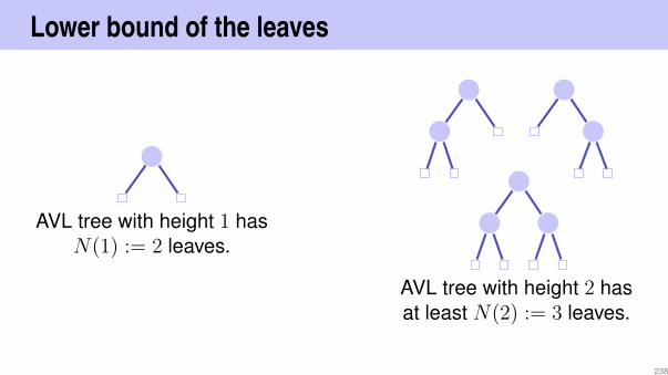
Lower bound of the leaves
AVL tree with height 1 hasN(1) := 2 leaves.
AVL tree with height 2 hasat least N(2) := 3 leaves.
238

Lower bound of the leaves for h > 2
Height of one subtree ≥ h− 1.Height of the other subtree ≥ h− 2.
Minimal number of leaves N(h) is
N(h) = N(h− 1) +N(h− 2)
v
Tl(v)
Tr(v)
h− 2 h− 1
h
Overal we have N(h) = Fh+2 with Fibonacci-numbers F0 := 0,F1 := 1, Fn := Fn−1 + Fn−2 for n > 1.
239
Fibonacci Numbers, closed Form
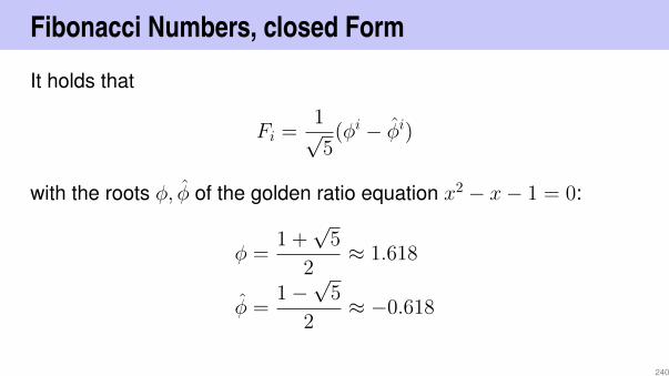
It holds that
Fi =1√5
(φi − φi)
with the roots φ, φ of the golden ratio equation x2 − x− 1 = 0:
φ =1 +√
5
2≈ 1.618
φ =1−√
5
2≈ −0.618
240

[Fibonacci Numbers, Inductive Proof]Fi
!= 1√
5(φi − φi) [∗]
(φ = 1+
√5
2 , φ = 1−√5
2
).
1 Immediate for i = 0, i = 1.
2 Let i > 2 and claim [∗] true for all Fj , j < i.
Fidef= Fi−1 + Fi−2
[∗]=
1√5
(φi−1 − φi−1) +1√5
(φi−2 − φi−2)
=1√5
(φi−1 + φi−2)− 1√5
(φi−1 + φi−2) =1√5φi−2(φ+ 1)− 1√
5φi−2(φ+ 1)
(φ, φ fulfil x+ 1 = x2)
=1√5φi−2(φ2)− 1√
5φi−2(φ2) =
1√5
(φi − φi).
(not shown in class) 241
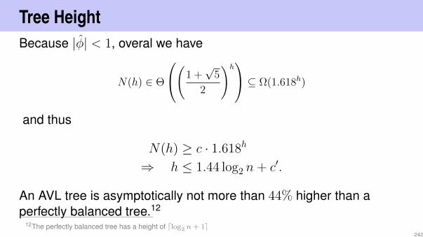
Tree HeightBecause |φ| < 1, overal we have
N(h) ∈ Θ
(1 +√
5
2
)h ⊆ Ω(1.618h)
and thus
N(h) ≥ c · 1.618h
⇒ h ≤ 1.44 log2 n+ c′.
An AVL tree is asymptotically not more than 44% higher than aperfectly balanced tree.12
12The perfectly balanced tree has a height of dlog2 n + 1e242

Insertion
Balance
Keep the balance stored in each nodeRe-balance the tree in each update-operation
New node n is inserted:
Insert the node as for a search tree.Check the balance condition increasing from n to the root.
243

Balance at Insertion Point
=⇒
+1 0p p
n
case 1: bal(p) = +1
=⇒
−1 0p p
n
case 2: bal(p) = −1
Finished in both cases because the subtree height did not change
244

Balance at Insertion Point
=⇒
0 +1p p
n
case 3.1: bal(p) = 0 right
=⇒
0 −1p p
n
case 3.2: bal(p) = 0, left
Not finished in both case. Call of upin(p)
245
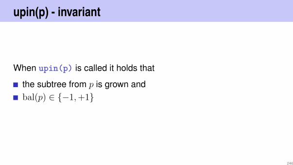
upin(p) - invariant
When upin(p) is called it holds that
the subtree from p is grown andbal(p) ∈ −1,+1
246

upin(p)
Assumption: p is left son of pp13
=⇒
pp +1 pp 0
p p
case 1: bal(pp) = +1, done.
=⇒
pp 0 pp −1
p p
case 2: bal(pp) = 0, upin(pp)
In both cases the AVL-Condition holds for the subtree from pp
13If p is a right son: symmetric cases with exchange of +1 and −1247

upin(p)Assumption: p is left son of pp
pp −1
p
case 3: bal(pp) = −1,
This case is problematic: adding n to the subtree from pp hasviolated the AVL-condition. Re-balance!
Two cases bal(p) = −1, bal(p) = +1248

Rotationscase 1.1 bal(p) = −1. 14
y
x
t1
t2
t3
pp −2
p −1
h
h− 1
h− 1
h + 2 h
=⇒rotation
right
x
y
t1 t2 t3
pp 0
p 0
h h− 1 h− 1
h + 1 h + 1
14p right son: ⇒ bal(pp) = bal(p) = +1, left rotation249

Rotationscase 1.1 bal(p) = −1. 15
z
x
y
t1 t2 t3
t4
pp −2
p +1
h −1/ + 1
h− 1
h− 1
h− 2
h− 2
h− 1
h− 1
h + 2 h
=⇒doublerotationleft-right
y
x z
t1t2 t3
t4
pp 0
0/− 1 +1/0
h− 1 h− 1
h− 2
h− 2
h− 1
h− 1
h + 1
15p right son⇒ bal(pp) = +1, bal(p) = −1, double rotation right left250

Analysis
Tree height: O(log n).Insertion like in binary search tree.Balancing via recursion from node to the root. Maximal pathlenght O(log n).
Insertion in an AVL-tree provides run time costs of O(log n).
251

DeletionCase 1: Children of node n are both leaves Let p be parent node ofn. ⇒ Other subtree has height h′ = 0, 1 or 2.
h′ = 1: Adapt bal(p).h′ = 0: Adapt bal(p). Call upout(p).h′ = 2: Rebalanciere des Teilbaumes. Call upout(p).
p
n
h = 0, 1, 2
−→
p
h = 0, 1, 2
252

Deletion
Case 2: one child k of node n is an inner node
Replace n by k. upout(k)
p
n
k −→
p
k
253

Deletion
Case 3: both children of node n are inner nodes
Replace n by symmetric successor. upout(k)Deletion of the symmetric successor is as in case 1 or 2.
254

upout(p)
Let pp be the parent node of p.
(a) p left child of pp
1 bal(pp) = −1 ⇒ bal(pp)← 0. upout(pp)2 bal(pp) = 0 ⇒ bal(pp)← +1.3 bal(pp) = +1⇒ next slides.
(b) p right child of pp: Symmetric cases exchanging +1 and −1.
255
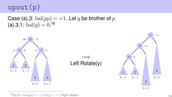
upout(p)Case (a).3: bal(pp) = +1. Let q be brother of p(a).3.1: bal(q) = 0.16
ypp +1
xp 0 zq 0
1 2
3 4
h− 1 h− 1
h + 1 h + 1
=⇒Left Rotate(y)
z −1
y +1
x 0
1 2
3
4
h− 1 h− 1
h + 1
h + 1
16(b).3.1: bal(pp) = −1, bal(q) = −1, Right rotation 256

upout(p)Case (a).3: bal(pp) = +1. (a).3.2: bal(q) = +1.17
ypp +1
xp 0 zq +1
1 2
3
4
h− 1 h− 1
h
h + 1
=⇒Left Rotate(y)
z 0r
y 0
x 0
1 2 3 4
h− 1 h− 1 h h + 1
plus upout(r).
17(b).3.2: bal(pp) = −1, bal(q) = +1, Right rotation+upout257

upout(p)Case (a).3: bal(pp) = +1. (a).3.3: bal(q) = −1.18
ypp +1
xp 0 zq −1
w
1 2
3 4
5h− 1 h− 1
h
=⇒Rotate right(z) left (y)
w 0r
y 0
x
z
0
1 2 3 4 5
h− 1 h− 1 h
plus upout(r).18(b).3.3: bal(pp) = −1, bal(q) = −1, left-right rotation + upout
258

Conclusion
AVL trees have worst-case asymptotic runtimes of O(log n) forsearching, insertion and deletion of keys.Insertion and deletion is relatively involved and an overkill forreally small problems.
259

12. Dynamic Programming
Memoization, Optimal Substructure, Overlapping Sub-Problems,Dependencies, General Procedure. Examples: Rod Cutting,Rabbits, Edit Distance
[Ottman/Widmayer, Kap. 7.1, 7.4, Cormen et al, Kap. 15]
260

Fibonacci Numbers
(again)
Fn :=
n if n < 2
Fn−1 + Fn−2 if n ≥ 2.
Analysis: why ist the recursive algorithm so slow?
261

Algorithm FibonacciRecursive(n)
Input: n ≥ 0Output: n-th Fibonacci number
if n < 2 thenf ← n
elsef ← FibonacciRecursive(n− 1) + FibonacciRecursive(n− 2)
return f
262

Analysis
T (n): Number executed operations.
n = 0, 1: T (n) = Θ(1)
n ≥ 2: T (n) = T (n− 2) + T (n− 1) + c.
T (n) = T (n− 2) + T (n− 1) + c ≥ 2T (n− 2) + c ≥ 2n/2c′ = (√
2)nc′
Algorithm is exponential in n.
263

Reason (visual)
F47
F46
F45
F44 F43
F44
F43 F42
F45
F44
F43 F42
F43
F42 F41
Nodes with same values are evaluated (too) often.
264

Memoization
Memoization (sic) saving intermediate results.
Before a subproblem is solved, the existence of the correspondingintermediate result is checked.If an intermediate result exists then it is used.Otherwise the algorithm is executed and the result is savedaccordingly.
265

Memoization with Fibonacci
F47
F46
F45
F44 F43
F44
F45
Rechteckige Knoten wurden bereits ausgewertet.
266

Algorithm FibonacciMemoization(n)
Input: n ≥ 0Output: n-th Fibonacci number
if n ≤ 2 thenf ← 1
else if ∃memo[n] thenf ← memo[n]
elsef ← FibonacciMemoization(n− 1) + FibonacciMemoization(n− 2)memo[n]← f
return f
267

Analysis
Computational complexity:
T (n) = T (n− 1) + c = ... = O(n).
because after the call to f(n− 1), f(n− 2) has already beencomputed.
A different argument: f(n) is computed exactly once recursively foreach n. Runtime costs: n calls with Θ(1) costs per call n · c ∈ Θ(n).The recursion vanishes from the running time computation.
Algorithm requires Θ(n) memory.19
19But the naive recursive algorithm also requires Θ(n) memory implicitly.268

Looking closer ...
... the algorithm computes the values of F1, F2, F3,. . . in thetop-down approach of the recursion.
Can write the algorithm bottom-up. This is characteristic for dynamicprogramming.
269

Algorithm FibonacciBottomUp(n)
Input: n ≥ 0Output: n-th Fibonacci number
F [1]← 1F [2]← 1for i← 3, . . . , n do
F [i]← F [i− 1] + F [i− 2]
return F [n]
270

Dynamic Programming: Idea
Divide a complex problem into a reasonable number ofsub-problemsThe solution of the sub-problems will be used to solve the morecomplex problemIdentical problems will be computed only once
271

Dynamic Programming Consequence
Identical problems will be computed only once
⇒ Results are saved
We trade spee against
memory consumption
272

Dynamic Programming: Description
1 Use a DP-table with information to the subproblems.Dimension of the entries? Semantics of the entries?
2 Computation of the base casesWhich entries do not depend on others?
3 Determine computation order.In which order can the entries be computed such that dependencies arefulfilled?
4 Read-out the solutionHow can the solution be read out from the table?
Runtime (typical) = number entries of the table times required operations per entry.
273

Dynamic Programing: Description with the example
1Dimension of the table? Semantics of the entries?n× 1 table. nth entry contains nth Fibonacci number.
2Which entries do not depend on other entries?Values F1 and F2 can be computed easily and independently.
3What is the execution order such that required entries are always available?Fi with increasing i.
4Wie kann sich Lösung aus der Tabelle konstruieren lassen?Fn ist die n-te Fibonacci-Zahl.
274

Dynamic Programming = Divide-And-Conquer ?
In both cases the original problem can be solved (more easily) byutilizing the solutions of sub-problems. The problem providesoptimal substructure.Divide-And-Conquer algorithms (such as Mergesort):sub-problems are independent; their solutions are required onlyonce in the algorithm.DP: sub-problems are dependent. The problem is said to haveoverlapping sub-problems that are required multiple-times in thealgorithm.In order to avoid redundant computations, results are tabulated.For sub-problems there must not be any circular dependencies.
275

Rod Cutting
Rods (metal sticks) are cut and sold.Rods of length n ∈ N are available. A cut does not provide anycosts.For each length l ∈ N, l ≤ n known is the value vl ∈ R+
Goal: cut the rods such (into k ∈ N pieces) that
k∑i=1
vli is maximized subject tok∑i=1
li = n.
276

Rod Cutting: Example
Possibilities to cut a rod of length 4 (without permutations)
Length 0 1 2 3 4Price 0 2 3 8 9
⇒ Best cut: 3 + 1 with value 10.
277
Wie findet man den DP Algorithms
0 Exact formulation of the wanted solution1 Define sub-problems (and compute the cardinality)2 Guess / Enumerate (and determine the running time for
guessing)3 Recursion: relate sub-problems4 Memoize / Tabularize. Determine the dependencies of the
sub-problems5 Solve the problem
Running time = #sub-problems × time/sub-problem
278

Structure of the problem0 Wanted: rn = maximal value of rod (cut or as a whole) with
length n.1 sub-problems: maximal value rk for each 0 ≤ k < n
2 Guess the length of the first piece3 Recursion
rk = max vi + rk−i : 0 < i ≤ k , k > 0
r0 = 0
4 Dependency: rk depends (only) on values vi, 1 ≤ i ≤ k and theoptimal cuts ri, i < k
5 Solution in rn279

Algorithm RodCut(v,n)
Input: n ≥ 0, Prices vOutput: best value
q ← 0if n > 0 then
for i← 1, . . . , n doq ← maxq, vi + RodCut(v, n− i);
return q
Running time T (n) =∑n−1
i=0 T (i) + c ⇒20 T (n) ∈ Θ(2n)
20T (n) = T (n− 1) +∑n−2
i=0 T (i) + c = T (n− 1) + (T (n− 1)− c) + c = 2T (n− 1) (n > 0)280

Recursion Tree
5
4
3
2
1
1
2
1
1
3
2
1
1
2
1
1
281

Algorithm RodCutMemoized(m, v, n)Input: n ≥ 0, Prices v, Memoization Table mOutput: best value
q ← 0if n > 0 then
if ∃ m[n] thenq ← m[n]
elsefor i← 1, . . . , n do
q ← maxq, vi + RodCutMemoized(m, v, n− i);m[n]← q
return q
Running time∑n
i=1 i = Θ(n2)
282

Subproblem-Graph
Describes the mutual dependencies of the subproblems
4 3 2 1 0
and must not contain cycles
283

Construction of the Optimal Cut
During the (recursive) computation of the optimal solution for eachk ≤ n the recursive algorithm determines the optimal length of thefirst rodStore the lenght of the first rod in a separate table of length n
284

Bottom-up Description with the example
1Dimension of the table? Semantics of the entries?n× 1 table. nth entry contains the best value of a rod of length n.
2Which entries do not depend on other entries?Value r0 is 0
3What is the execution order such that required entries are always available?ri, i = 1, . . . , n.
4Wie kann sich Lösung aus der Tabelle konstruieren lassen?rn is the best value for the rod of length n.
285

Rabbit!
A rabbit sits on cite (1, 1)of an n × n grid. It canonly move to east or south.On each pathway there isa number of carrots. Howmany carrots does the rab-bit collect maximally?
1, 1
1, 2
1, 3
1, 4
2, 1
2, 2
2, 3
2, 4
3, 1
3, 2
3, 3
3, 4
4, 1
4, 2
4, 3
4, 4
0
1
1
1
2
4
4
0
0
1
2
4
0
3
1
3
0
0
4
4
1
1
0
4
286

Rabbit!
Number of possible paths?Choice of n− 1 ways to south out of2n− 2 ways overal.(
2n− 2
n− 1
)∈ Ω(2n)
⇒ No chance for a naive algorithmThe path 100011
(1:to south, 0: to east)
287

Recursion
Wanted: T0,0 = maximal number carrots from (0, 0) to (n, n).
Let w(i,j)−(i′,j′) number of carrots on egde from (i, j) to (i′, j′).
Recursion (maximal number of carrots from (i, j) to (n, n)
Tij =
maxw(i,j)−(i,j+1) + Ti,j+1, w(i,j)−(i+1,j) + Ti+1,j, i < n, j < n
w(i,j)−(i,j+1) + Ti,j+1, i = n, j < n
w(i,j)−(i+1,j) + Ti+1,j, i < n, j = n
0 i = j = n
288

Graph of Subproblem Dependencies
(1, 1)
(1, 2)
(1, 3)
(1, 4)
(2, 1)
(2, 2)
(2, 3)
(2, 4)
(3, 1)
(3, 2)
(3, 3)
(3, 4)
(4, 1)
(4, 2)
(4, 3)
(4, 4)
289

Bottom-up Description with the example
1
Dimension of the table? Semantics of the entries?Table T with size n× n. Entry at i, j provides the maximal number of carrotsfrom (i, j) to (n, n).
2Which entries do not depend on other entries?Value Tn,n is 0
3
What is the execution order such that required entries are always available?Ti,j with i = n 1 and for each i: j = n 1, (or vice-versa: j = n 1 andfor each j: i = n 1).
4Wie kann sich Lösung aus der Tabelle konstruieren lassen?T1,1 provides the maximal number of carrots.
290

DNA - Comparison (Star Trek)
291
DNA - Comparison
DNA consists of sequences of four different nucleotides AdenineGuanine Thymine CytosineDNA sequences (genes) thus can be described with strings of A,G, T and C.Possible comparison of two genes: determine the longestcommon subsequence
The longest common subsequence problem is a special case of theminimal edit distance problem. The following slides are therefore notpresented in the lectures.
292

[Longest common subsequence]
Subsequences of a string:Subsequences(KUH): (), (K), (U), (H), (KU), (KH), (UH),(KUH)
Problem:
Input: two strings A = (a1, . . . , am), B = (b1, . . . , bn) with lengthsm > 0 and n > 0.Wanted: Longest common subsequecnes (LCS) of A and B.
(not shown in class) 293

[Longest Common Subsequence]
Examples:LGT(IGEL,KATZE)=E, LGT(TIGER,ZIEGE)=IGE
Ideas to solve?
T I G E RZ I E G E
(not shown in class) 294

[Recursive Procedure]Assumption: solutions L(i, j) known for A[1, . . . , i] and B[1, . . . , j]for all 1 ≤ i ≤ m and 1 ≤ j ≤ n, but not for i = m and j = n.
T I G E RZ I E G E
Consider characters am, bn. Three possibilities:
1 A is enlarged by one whitespace. L(m,n) = L(m,n− 1)
2 B is enlarged by one whitespace. L(m,n) = L(m− 1, n)
3 L(m,n) = L(m− 1, n− 1) + δmn with δmn = 1 if am = bn andδmn = 0 otherwise
(not shown in class) 295

[Recursion]
L(m,n)← max L(m− 1, n− 1) + δmn, L(m,n− 1), L(m− 1, n)
for m,n > 0 and base cases L(·, 0) = 0, L(0, ·) = 0.
∅ Z I E G E∅ 0 0 0 0 0 0T 0 0 0 0 0 0I 0 0 1 1 1 1G 0 0 1 1 2 2E 0 0 1 2 2 3R 0 0 1 2 2 3
(not shown in class) 296

[Dynamic Programming algorithm LCS]
1
Dimension of the table? Semantics?Table L[0, . . . ,m][0, . . . , n]. L[i, j]: length of a LCS of the strings (a1, . . . , ai)and (b1, . . . , bj)
2
Computation of an entry
L[0, i]← 0 ∀0 ≤ i ≤ m, L[j, 0]← 0 ∀0 ≤ j ≤ n. Computation of L[i, j]otherwise via L[i, j] = max(L[i− 1, j − 1] + δij, L[i, j − 1], L[i− 1, j]).
(not shown in class) 297

[Dynamic Programming algorithm LCS]
3Computation orderRows increasing and within columns increasing (or the other way round).
4
Reconstruct solution?Start with j = m, i = n. If ai = bj then output ai and continue with(j, i)← (j − 1, i− 1); otherwise, if L[i, j] = L[i, j − 1] continue withj ← j − 1 otherwise, if L[i, j] = L[i− 1, j] continue with i← i− 1 .Terminate for i = 0 or j = 0.
(not shown in class) 298

[Analysis LCS]
Number table entries: (m+ 1) · (n+ 1).Constant number of assignments and comparisons each. Numbersteps: O(mn)
Determination of solition: decrease i or j. Maximally O(n+m)steps.
Runtime overal:O(mn).
(not shown in class) 299

Minimal Editing Distance
Editing distance of two sequences An = (a1, . . . , am),Bm = (b1, . . . , bm).
Editing operations:
Insertion of a characterDeletion of a characterReplacement of a character
Question: how many editing operations at least required in order totransform string A into string B.
TIGER ZIGER ZIEGER ZIEGE
300
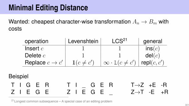
Minimal Editing Distance
Wanted: cheapest character-wise transformation An → Bm withcosts
operation Levenshtein LCS21 generalInsert c 1 1 ins(c)Delete c 1 1 del(c)Replace c→ c′ 1(c 6= c′) ∞ · 1(c 6= c′) repl(c, c′)
BeispielT I G E RZ I E G E
T I _ G E RZ I E G E _
T→Z +E -RZ→T -E +R
21Longest common subsequence – A special case of an editing problem301

DP0 E(n,m) = mimimum number edit operations (ED cost)a1...n → b1...m
1 Subproblems E(i, j) = ED von a1...i. b1...j. #SP = n ·m2 Guess CostsΘ(1)
a1..i → a1...i−1 (delete)a1..i → a1...ibj (insert)a1..i → a1...i1bj (replace)
3 Rekursion
E(i, j) = min
del(ai) + E(i− 1, j),
ins(bj) + E(i, j − 1),
repl(ai, bj) + E(i− 1, j − 1)302

DP
4 Dependencies
⇒ Computation from left top to bottom right. Row- orcolumn-wise.
5 Solution in E(n,m)
303

Example (Levenshtein Distance)
E[i, j]← minE[i−1, j]+1, E[i, j−1]+1, E[i−1, j−1]+1(ai 6= bj)
∅ Z I E G E
∅ 0 1 2 3 4 5T 1 1 2 3 4 5I 2 2 1 2 3 4G 3 3 2 2 2 3E 4 4 3 2 3 2R 5 5 4 3 3 3
Editing steps: from bottom right to top left, following the recursion.Bottom-Up description of the algorithm: exercise
304

Bottom-Up DP algorithm ED]
1
Dimension of the table? Semantics?Table E[0, . . . ,m][0, . . . , n]. E[i, j]: minimal edit distance of the strings(a1, . . . , ai) and (b1, . . . , bj)
2
Computation of an entry
E[0, i]← i ∀0 ≤ i ≤ m, E[j, 0]← i ∀0 ≤ j ≤ n. Computation of E[i, j]otherwise via E[i, j] =mindel(ai) +E(i− 1, j), ins(bj) +E(i, j − 1), repl(ai, bj) +E(i− 1, j − 1)
305

Bottom-Up DP algorithm ED
3Computation orderRows increasing and within columns increasing (or the other way round).
4
Reconstruct solution?Start with j = m, i = n. If E[i, j] = repl(ai, bj) + E(i− 1, j − 1) then outputai → bj and continue with (j, i)← (j − 1, i− 1); otherwise, ifE[i, j] = del(ai) + E(i− 1, j) output del(ai) and continue with j ← j − 1otherwise, if E[i, j] = ins(bj) + E(i, j − 1), continue with i← i− 1 .Terminate for i = 0 and j = 0.
306

13. Graphs
Notation, Representation, Graph Traversal (DFS, BFS), TopologicalSorting [Ottman/Widmayer, Kap. 9.1 - 9.4,Cormen et al, Kap. 22]
307
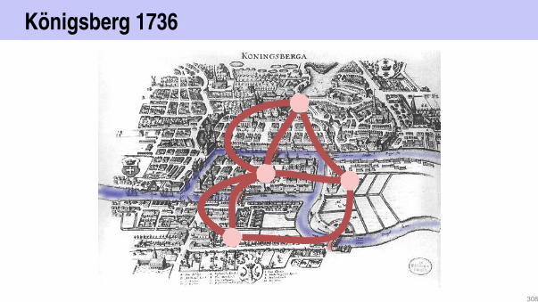
Konigsberg 1736
308

[Multi]Graph
A
B
D
C
edge
node
309

Cycles
Is there a cycle through the town (thegraph) that uses each bridge (each edge)exactly once?Euler (1736): no.Such a cycle is called Eulerian path.Eulerian path⇔ each node provides aneven number of edges (each node is of aneven degree).‘⇒” is straightforward, “⇐” ist a bit more difficult but still elementary.
A
B
D
C
310

Notation1
2 3
4 5
undirected
V =1, 2, 3, 4, 5E =1, 2, 1, 3, 2, 3, 2, 4,2, 5, 3, 4, 3, 5, 4, 5
1
2 3
4 5
directed
V =1, 2, 3, 4, 5E =(1, 3), (2, 1), (2, 5), (3, 2),
(3, 4), (4, 2), (4, 5), (5, 3)311

Notation
A directed graph consists of a set V = v1, . . . , vn of nodes(Vertices) and a set E ⊆ V × V of Edges. The same edges may notbe contained more than once.
1 2
3 4 5
loop
312
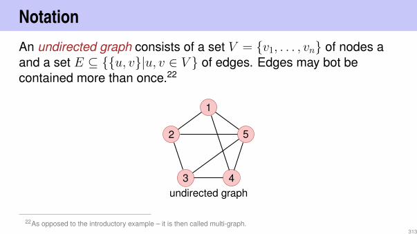
NotationAn undirected graph consists of a set V = v1, . . . , vn of nodes aand a set E ⊆ u, v|u, v ∈ V of edges. Edges may bot becontained more than once.22
1
2
3 4
5
undirected graph
22As opposed to the introductory example – it is then called multi-graph.313

Notation
An undirected graph G = (V,E) without loops where E comprisesall edges between pairwise different nodes is called complete.
1
2
3 4
5
a complete undirected graph
314

Notation
A graph where V can be partitioned into disjoint sets U and W suchthat each e ∈ E provides a node in U and a node in W is calledbipartite.
315

Notation
A weighted graph G = (V,E, c) is a graph G = (V,E) with an edgeweight function c : E → R. c(e) is called weight of the edge e.
0
1
2
3
4
5
2
1.5
4
1
4
3
316

NotationFor directed graphs G = (V,E)
w ∈ V is called adjacent to v ∈ V , if (v, w) ∈ EPredecessors of v ∈ V : N−(v) := u ∈ V |(u, v) ∈ E.Successors: N+(v) := u ∈ V |(v, u) ∈ E
N−(v) N+(v)
v
p1
p2
p3
s1
s2
317

Notation
For directed graphs G = (V,E)
In-Degree: deg−(v) = |N−(v)|,Out-Degree: deg+(v) = |N+(v)|
v
deg−(v) = 3, deg+(v) = 2
w
deg−(w) = 1, deg+(w) = 1
318

Notation
For undirected graphs G = (V,E):
w ∈ V is called adjacent to v ∈ V , if v, w ∈ ENeighbourhood of v ∈ V : N(v) = w ∈ V |v, w ∈ EDegree of v: deg(v) = |N(v)| with a special case for the loops:increase the degree by 2.
v
deg(v) = 5
w
deg(w) = 2
319

Relationship between node degrees and number ofedges
For each graph G = (V,E) it holds
1∑
v∈V deg−(v) =∑
v∈V deg+(v) = |E|, for G directed2∑
v∈V deg(v) = 2|E|, for G undirected.
320

Paths
Path: a sequence of nodes 〈v1, . . . , vk+1〉 such that for eachi ∈ 1 . . . k there is an edge from vi to vi+1 .Length of a path: number of contained edges k.Weight of a path (in weighted graphs):
∑ki=1 c((vi, vi+1)) (bzw.∑k
i=1 c(vi, vi+1))Simple path: path without repeating vertices
321

Connectedness
An undirected graph is called connected, if for eacheach pairv, w ∈ V there is a connecting path.A directed graph is called strongly connected, if for each pairv, w ∈ V there is a connecting path.A directed graph is called weakly connected, if the correspondingundirected graph is connected.
322

Simple Observations
generally: 0 ≤ |E| ∈ O(|V |2)connected graph: |E| ∈ Ω(|V |)complete graph: |E| = |V |·(|V |−1)
2 (undirected)
Maximally |E| = |V |2 (directed ),|E| = |V |·(|V |+1)2 (undirected)
323

Cycles
Cycle: path 〈v1, . . . , vk+1〉 with v1 = vk+1
Simple cycle: Cycle with pairwise different v1, . . . , vk, that doesnot use an edge more than once.Acyclic: graph without any cycles.
Conclusion: undirected graphs cannot contain cycles with length 2(loops have length 1)
324

Representation using a MatrixGraph G = (V,E) with nodes v1 . . . , vn stored as adjacency matrixAG = (aij)1≤i,j≤n with entries from 0, 1. aij = 1 if and only if edgefrom vi to vj.
1 2
4
3
5
0 1 1 1 00 0 0 0 00 1 0 1 10 0 0 0 00 0 1 0 1
Memory consumption Θ(|V |2). AG is symmetric, if G undirected.
325

Representation with a ListMany graphs G = (V,E) with nodesv1, . . . , vn provide much less than n2
edges. Representation with adjacencylist: Array A[1], . . . , A[n], Ai comprises alinked list of nodes in N+(vi).
1 2
4
3
5
1 2 3 4 5
2
3
4
2
4
5
3
5
Memory Consumption Θ(|V |+ |E|).326

Runtimes of simple Operations
Operation Matrix List
Find neighbours/successors of v ∈ V Θ(n) Θ(deg+ v)
find v ∈ V without neighbour/successor Θ(n2) Θ(n)
(u, v) ∈ E ? Θ(1) Θ(deg+ v)
Insert edge Θ(1) Θ(1)
Delete edge Θ(1) Θ(deg+ v)
327

Depth First Search
328

Graph Traversal: Depth First Search
Follow the path into its depth until nothing is left to visit.
a b c
d e f
g h i
aa bb cc
ffdd eeee
gg hh i
Order a, b, c, f, d, e, g, h, i
Adjazenzlistea b c d e f g h i
b c f e b h e
d f i
e
329

Colors
Conceptual coloring of nodes
white: node has not been discovered yet.grey: node has been discovered and is marked for traversal /being processed.black: node was discovered and entirely processed.
330

Algorithm Depth First visit DFS-Visit(G, v)
Input: graph G = (V,E), Knoten v.
v.color ← greyforeach w ∈ N+(v) do
if w.color = white thenDFS-Visit(G,w)
v.color ← black
Depth First Search starting from node v. Running time (withoutrecursion): Θ(deg+ v)
331

Algorithm Depth First visit DFS-Visit(G)
Input: graph G = (V,E)
foreach v ∈ V dov.color ← white
foreach v ∈ V doif v.color = white then
DFS-Visit(G,v)
Depth First Search for all nodes of a graph. Running time:Θ(|V |+
∑v∈V (deg+(v) + 1)) = Θ(|V |+ |E|).
332

Interpretation of the Colors
When traversing the graph, a tree (or Forest) is built. When nodesare discovered there are three cases
White node: new tree edgeGrey node: Zyklus (“back-egde”)Black node: forward- / cross edge
333

Breadth First Search
334

Graph Traversal: Breadth First Search
Follow the path in breadth and only then descend into depth.
a b c
d e f
g h i
aaaa bb
dd eee
cc
f
gg hh i
Order a, b, d, e, c, f, g, h, i
Adjazenzlistea b c d e f g h i
b c f e b h i
d f
e
335

(Iterative) BFS-Visit(G, v)Input: graph G = (V,E)
Queue Q← ∅v.color ← greyenqueue(Q, v)while Q 6= ∅ do
w ← dequeue(Q)foreach c ∈ N+(w) do
if c.color = white thenc.color ← greyenqueue(Q, c)
w.color ← black
Algorithm requires extra space of O(|V |).336

Main program BFS-Visit(G)
Input: graph G = (V,E)
foreach v ∈ V dov.color ← white
foreach v ∈ V doif v.color = white then
BFS-Visit(G,v)
Breadth First Search for all nodes of a graph. Running time:Θ(|V |+ |E|).
337

Topological Sorting
Evaluation Order?338

Topological Sorting
Topological Sorting of an acyclic directed graph G = (V,E):
Bijective mappingord : V → 1, . . . , |V |
such thatord(v) < ord(w) ∀ (v, w) ∈ E.
Identify i with Element vi := ord1(i). Topological sorting =〈v1, . . . , v|V |〉.
339

(Counter-)Examples
1
2
3 4
5
Cyclic graph: cannot be sorted topologically.
Unterhose Hose
Socken Schuhe
Unterhemd Pullover
Mantel
Uhr
A possible toplogical sorting of the graph:Unterhemd,Pullover,Unterhose,Uhr,Hose,Mantel,Socken,Schuhe
340

Observation
TheoremA directed graph G = (V,E) permits a topological sorting if and onlyif it is acyclic.
Proof “⇒”: If G contains a cycle it cannot permit a topologicalsorting, because in a cycle 〈vi1, . . . , vim〉 it would hold thatvi1 < · · · < vim < vi1.
341

Inductive Proof Opposite Direction
Base case (n = 1): Graph with a single node without loop can besorted topologically, setord(v1) = 1.Hypothesis: Graph with n nodes can be sorted topologicallyStep (n→ n+ 1):
1 G contains a node vq with in-degree deg−(vq) = 0. Otherwise iterativelyfollow edges backwards – after at most n+ 1 iterations a node would berevisited. Contradiction to the cycle-freeness.
2 Graph without node vq and without its edges can be topologically sortedby the hypothesis. Now use this sorting and set ord(vi)← ord(vi) + 1 forall i 6= q and set ord(vq)← 1.
342

Preliminary Sketch of an Algorithm
Graph G = (V,E). d← 1
1 Traverse backwards starting from any node until a node vq within-degree 0 is found.
2 If no node with in-degree 0 found after n stepsm, then the graphhas a cycle.
3 Set ord(vq)← d.4 Remove vq and his edges from G.5 If V 6= ∅ , then d← d+ 1, go to step 1.
Worst case runtime: Θ(|V |2).
343

Improvement
Idea?
Compute the in-degree of all nodes in advance and traverse thenodes with in-degree 0 while correcting the in-degrees of followingnodes.
344

Algorithm Topological-Sort(G)Input: graph G = (V,E).Output: Topological sorting ord
Stack S ← ∅foreach v ∈ V do A[v]← 0foreach (v, w) ∈ E do A[w]← A[w] + 1 // Compute in-degreesforeach v ∈ V with A[v] = 0 do push(S, v) // Memorize nodes with in-degree
0i← 1while S 6= ∅ do
v ← pop(S); ord[v]← i; i← i+ 1 // Choose node with in-degree 0foreach (v, w) ∈ E do // Decrease in-degree of successors
A[w]← A[w]− 1if A[w] = 0 then push(S,w)
if i = |V |+ 1 then return ord else return “Cycle Detected”345
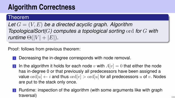
Algorithm CorrectnessTheoremLet G = (V,E) be a directed acyclic graph. AlgorithmTopologicalSort(G) computes a topological sorting ord for G withruntime Θ(|V |+ |E|).
Proof: follows from previous theorem:
1 Decreasing the in-degree corresponds with node removal.
2 In the algorithm it holds for each node v with A[v] = 0 that either the nodehas in-degree 0 or that previously all predecessors have been assigned avalue ord[u]← i and thus ord[v] > ord[u] for all predecessors u of v. Nodesare put to the stack only once.
3 Runtime: inspection of the algorithm (with some arguments like with graphtraversal) 346

Algorithm Correctness
TheoremLet G = (V,E) be a directed graph containing a cycle. AlgorithmTopologicalSort(G) terminates within Θ(|V |+ |E|) steps and detectsa cycle.
Proof: let 〈vi1 , . . . , vik〉 be a cycle in G. In each step of the algorithm remainsA[vij ] ≥ 1 for all j = 1, . . . , k. Thus k nodes are never pushed on the stack undtherefore at the end it holds that i ≤ V + 1− k.
The runtime of the second part of the algorithm can become shorter. But thecomputation of the in-degree costs already Θ(|V |+ |E|).
347

14. Shortest Paths
Motivation, Dijkstra’s algorithm on distance graphs, Bellman-FordAlgorithm
[Ottman/Widmayer, Kap. 9.5.1-9.5.2 Cormen et al, Kap. 24.1-24.3]
348

River Crossing (Missionaries and Cannibals)Problem: Three cannibals and three missionaries are standing at ariver bank. The available boat can carry two people. At no time mayat any place (banks or boat) be more cannibals than missionaries.How can the missionaries and cannibals cross the river as fast aspossible? 23
K K K
M M MB
23There are slight variations of this problem. It is equivalent to the jealous husbands problem.349

Problem as Graph
Enumerate permitted configurations as nodes and connect themwith an edge, when a crossing is allowed. The problem thenbecomes a shortest path problem.
Example
links rechtsMissionare 3 0Kannibalen 3 0Boot x
links rechtsMissionare 2 1Kannibalen 2 1Boot x
Überfahrt möglich
6 Personen am linken Ufer 4 Personen am linken Ufer
350

The whole problem as a graph
3 03 0x
3 02 1x
3 01 2x
3 00 3x
2 12 1x
1 21 2x
0 31 2x
0 32 1x
0 33 0x
6 5 4 3 4 2 1 2 3
3 02 1
x
3 01 2
x
3 00 3
x
2 12 1
x
1 21 2
x
0 31 2
x
0 32 1
x
0 33 0
x
0 30 3
x
5 4 3 4 2 1 2 3 0
351

Another Example: Mystic Square
Want to find the fastest solution for
2 4 67 5 31 8
1 2 34 5 67 8
352

Problem as Graph1 2 34 5 67 8
1 2 34 5 67 8
1 2 34 5 6
7 8
1 2 34 57 8 6
1 2 34 57 8 6
1 2 34 8 57 6
1 2 34 5
7 8 6
2 4 67 5 31 8
353
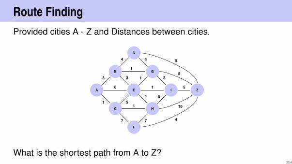
Route FindingProvided cities A - Z and Distances between cities.
A
B
C
D
E
F
G
H
I Z
3
1
6
4
1
3
5
7
1
4 5
1
4
1
7 4
38
5
10
5
What is the shortest path from A to Z?354

Simplest CaseConstant edge weight 1 (wlog)
Solution: Breadth First Search
S
t
355

Weighted GraphsGiven: G = (V,E, c), c : E → R, s, t ∈ V .Wanted: Length (weight) of a shortest path from s to t.Path: p = 〈s = v0, v1, . . . , vk = t〉, (vi, vi+1) ∈ E (0 ≤ i < k)Weight: c(p) :=
∑k−1i=0 c((vi, vi+1)).
S
t2 1
3
2
1
Path with weight 9
356

Shortest Paths
Notation: we write
up v oder p : u v
and mean a path p from u to v
Notation: δ(u, v) = weight of a shortest path from u to v:
δ(u, v) =
∞ no path from u to vminc(p) : u
p v otherwise
357
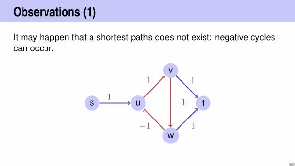
Observations (1)
It may happen that a shortest paths does not exist: negative cyclescan occur.
s u
v
w
t1
1
−1
−1
1
1
358

Observations (2)
There can be exponentially many paths.
s
t
(at least 2|V |/2 paths from s to t)
⇒ To try all paths is too inefficient
359

Observations (3)Triangle Inequality
For all s, u, v ∈ V :
δ(s, v) ≤ δ(s, u) + δ(u, v)
s
u
v
A shortest path from s to v cannot be longer than a shortest path from s to v thathas to include u
360

Observations (4)
Optimal Substructure
Sub-paths of shortest paths are shortest paths. Let p = 〈v0, . . . , vk〉be a shortest path from v0 to vk. Then each of the sub-pathspij = 〈vi, . . . , vj〉 (0 ≤ i < j ≤ k) is a shortest path from vi to vj.
u x y vp p
q
p
If not, then one of the sub-paths could be shortened which immediately leads to acontradiction.
361

Observations (5)
Shortest paths do not contain cycles
1 Shortest path contains a negative cycle: there is no shortest path,contradiction
2 Path contains a positive cycle: removing the cycle from the path will reducethe weight. Contradiction.
3 Path contains a cycle with weight 0: removing the cycle from the path will notchange the weight. Remove the cycle (convention).
362

Ingredients of an AlgorithmWanted: shortest paths from a starting node s.
Weight of the shortest path found so far
ds : V → R
At the beginning: ds[v] =∞ for all v ∈ V .Goal: ds[v] = δ(s, v) for all v ∈ V .Predecessor of a node
πs : V → V
Initially πs[v] undefined for each node v ∈ V363

General Algorithm
1 Initialise ds and πs: ds[v] =∞, πs[v] = null for each v ∈ V2 Set ds[s]← 0
3 Choose an edge (u, v) ∈ ERelaxiere (u, v):
if ds[v] > d[u] + c(u, v) thends[v]← ds[u] + c(u, v)πs[v]← u
4 Repeat 3 until nothing can be relaxed any more.(until ds[v] ≤ ds[u] + c(u, v) ∀(u, v) ∈ E)
364

It is Safe to RelaxAt any time in the algorithm above it holds
ds[v] ≥ δ(s, v) ∀v ∈ V
In the relaxation step:
δ(s, v) ≤ δ(s, u) + δ(u, v) [Triangle Inequality].δ(s, u) ≤ ds[u] [Induction Hypothesis].δ(u, v) ≤ c(u, v) [Minimality of δ]
⇒ ds[u] + c(u, v) ≥ δ(s, v)
⇒ minds[v], ds[u] + c(u, v) ≥ δ(s, v)
365

Central Question
How / in which order should edges be chosen in above algorithm?
366

Special Case: Directed Acyclic Graph (DAG)
DAG⇒ topological sorting returns optimal visiting order
s
v1
v2
v3
v4
v5
v6
v7
v82
4
−3
1
−1
2
−2
2
−2
2
3
−10
2
4
−1
−2
0
−4
3
−6
Top. Sort: ⇒ Order s, v1, v2, v3, v4, v6, v5, v8, v7.367

Assumption (preliminary)
s
a
b
c
d
e
2
3
2
6
1
3
1
1
All weights of G are positive.
368
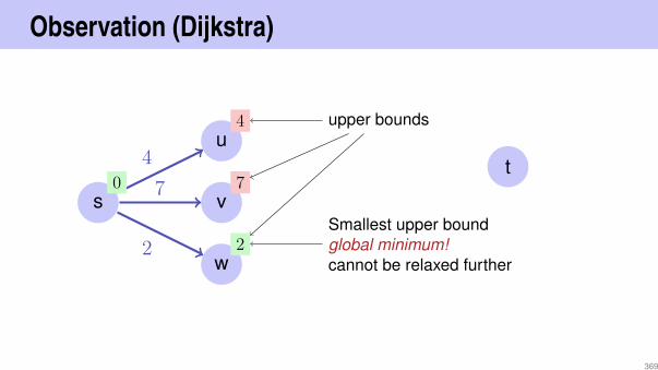
Observation (Dijkstra)
s
u
v
w
4
7
2
t0
4
7
2
upper bounds
Smallest upper boundglobal minimum!cannot be relaxed further
369

Basic Idea
Set V of nodes is partitioned intothe set M of nodes for which ashortest path from s is already known,the set R =
⋃v∈M N+(v) \M of
nodes where a shortest path is not yetknown but that are accessible directlyfrom M ,the set U = V \ (M ∪R) of nodes thathave not yet been considered.
s
2
2
5
3
5
2
1
2
370

Induction
Induction over |M |: choose nodes fromR with smallest upper bound. Add r to Mand update R and U accordingly.
Correctness: if within the “wavefront” anode with minimal weight w has beenfound then no path over later nodes (pro-viding weight ≥ d) can provide any im-provement.
s
2
2
5
3
5
2
1
2
371

Algorithm Dijkstra(G, s)Input: Positively weighted Graph G = (V,E, c), starting point s ∈ V ,Output: Minimal weights d of the shortest paths and corresponding predecessor
node for each node.
foreach u ∈ V dods[u]←∞; πs[u]← null
ds[s]← 0; R← swhile R 6= ∅ do
u← ExtractMin(R)foreach v ∈ N+(u) do
if ds[u] + c(u, v) < ds[v] thends[v]← ds[u] + c(u, v)πs[v]← uR← R ∪ v
372

Example
s
a
b
c
d
e
2
3
2
6
1
3
1
1
0
∞
∞
∞
∞
∞
ss
a
b
2
3
a c8
b d4
M = s, a, bR = c, dU = e
373

Implementation: Data Structure for R?Required operations:
Insert (add to R)ExtractMin (over R) and DecreaseKey (Update in R)foreach v ∈ N+(u) do
if ds[u] + c(u, v) < ds[v] thends[v]← ds[u] + c(u, v)πs[v]← uif v ∈ R then
DecreaseKey(R, v) // Update of a d(v) in the heap of Relse
R← R ∪ v // Update of d(v) in the heap of R
MinHeap!374
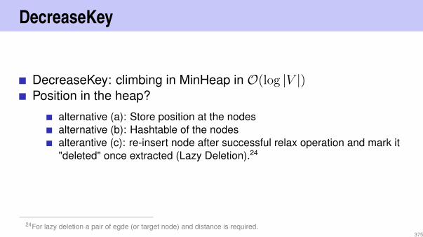
DecreaseKey
DecreaseKey: climbing in MinHeap in O(log |V |)Position in the heap?
alternative (a): Store position at the nodesalternative (b): Hashtable of the nodesalterantive (c): re-insert node after successful relax operation and mark it"deleted" once extracted (Lazy Deletion).24
24For lazy deletion a pair of egde (or target node) and distance is required.375
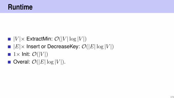
Runtime
|V |× ExtractMin: O(|V | log |V |)|E|× Insert or DecreaseKey: O(|E| log |V |)1× Init: O(|V |)Overal: O(|E| log |V |).
376

General Weighted GraphsRelaxing Step as before but with a return value:
Relax(u, v) (u, v ∈ V , (u, v) ∈ E)if ds[u] + c(u, v) < ds[v] then
ds[v]← ds[u] + c(u, v)πs[v]← ureturn true
return false
s
u
v
ds(u)
ds(v)
Problem: cycles with negative weights can shorten the path, ashortest path is not guaranteed to exist.
377

Dynamic Programming Approach (Bellman)
Induction over number of edges ds[i, v]: Shortest path from s to v viamaximally i edges.
ds[i, v] = minds[i− 1, v], min(u,v)∈E
(ds[i− 1, u] + c(u, v))
ds[0, s] = 0, ds[0, v] =∞ ∀v 6= s.
378

Dynamic Programming Approach (Bellman)
s · · · v · · · w0 0 ∞ ∞ ∞ ∞1 0 ∞ 7 ∞ −2... ... ... ... ... ...
n− 1 0 · · · · · · · · · · · ·
s
u
v
w
4
7
−2
Algorithm: Iterate over last row until the relaxation steps do notprovide any further changes, maximally n− 1 iterations. If stillchanges, then there is no shortest path.
379

Algorithm Bellman-Ford(G, s)Input: Graph G = (V,E, c), starting point s ∈ VOutput: If return value true, minimal weights d for all shortest paths from s,
otherwise no shortest path.
foreach u ∈ V dods[u]←∞; πs[u]← null
ds[s]← 0;for i← 1 to |V | do
f ← falseforeach (u, v) ∈ E do
f ← f ∨ Relax(u, v)
if f = false then return true
return false;
Runtime O(|E| · |V |).380

15. Minimum Spanning Trees
Motivation, Greedy, Algorithm Kruskal, General Rules, ADTUnion-Find, Algorithm Jarnik, Prim, Dijkstra, [Ottman/Widmayer,Kap. 9.6, 6.2, 6.1, Cormen et al, Kap. 23, 19]
381
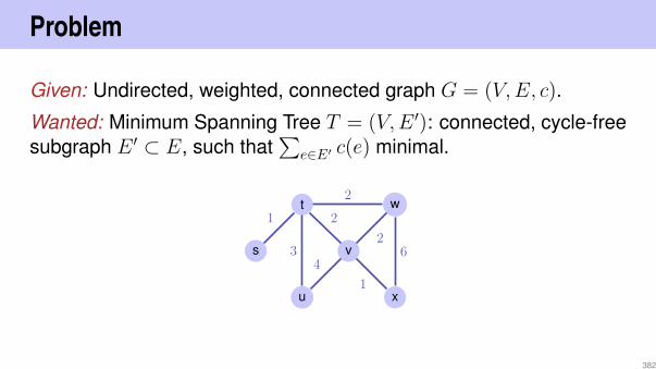
Problem
Given: Undirected, weighted, connected graph G = (V,E, c).
Wanted: Minimum Spanning Tree T = (V,E ′): connected, cycle-freesubgraph E ′ ⊂ E, such that
∑e∈E′ c(e) minimal.
s
t
u
v
w
x
1
1
2
43
2
26
382

Application Examples
Network-Design: find the cheapest / shortest network thatconnects all nodes.Approximation of a solution of the travelling salesman problem:find a round-trip, as short as possible, that visits each node once.25
25The best known algorithm to solve the TS problem exactly has exponential running time.383

Greedy Procedure
Greedy algorithms compute the solution stepwise choosing locallyoptimal solutions.Most problems cannot be solved with a greedy algorithm.The Minimum Spanning Tree problem can be solved with a greedystrategy.
384

Greedy Idea (Kruskal, 1956)
Construct T by adding the cheapest edge that does not generate acycle.
s
t
u
v
w
x
1
1
2
43
2
26
(Solution is not unique.)
385

Algorithm MST-Kruskal(G)
Input: Weighted Graph G = (V,E, c)Output: Minimum spanning tree with edges A.
Sort edges by weight c(e1) ≤ ... ≤ c(em)A← ∅for k = 1 to |E| do
if (V,A ∪ ek) acyclic thenA← A ∪ ek
return (V,A, c)
386

[Correctness]
At each point in the algorithm (V,A) is a forest, a set of trees.
MST-Kruskal considers each edge ek exactly once and eitherchooses or rejects ekNotation (snapshot of the state in the running algorithm)
A: Set of selected edgesR: Set of rejected edgesU : Set of yet undecided edges
(not shown in class) 387

[Cut]A cut of G is a partition S, V − S of V . (S ⊆ V ).
An edge crosses a cut when one of its endpoints is in S and theother is in V \ S.
S
V \ S
(not shown in class) 388

[Rules]
1 Selection rule: choose a cut that is not crossed by a selectededge. Of all undecided edges that cross the cut, select the onewith minimal weight.
2 Rejection rule: choose a circle without rejected edges. Of allundecided edges of the circle, reject those with minimal weight.
(not shown in class) 389
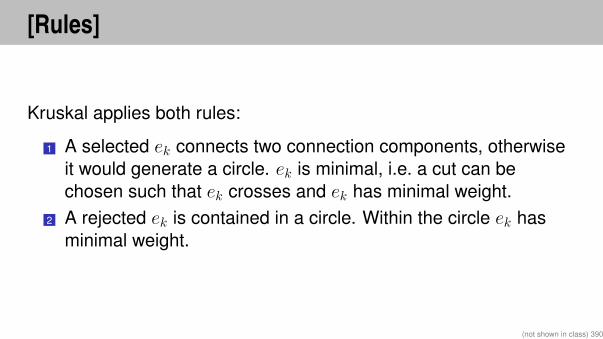
[Rules]
Kruskal applies both rules:
1 A selected ek connects two connection components, otherwiseit would generate a circle. ek is minimal, i.e. a cut can bechosen such that ek crosses and ek has minimal weight.
2 A rejected ek is contained in a circle. Within the circle ek hasminimal weight.
(not shown in class) 390

[Correctness]
TheoremEvery algorithm that applies the rules above in a step-wise manneruntil U = ∅ is correct.
Consequence: MST-Kruskal is correct.
(not shown in class) 391

[Selection invariant]
Invariant: At each step there is a minimal spanning tree that containsall selected and none of the rejected edges.
If both rules satisfy the invariant, then the algorithm is correct.Induction:
At beginning: U = E, R = A = ∅. Invariant obviously holds.Invariant is preserved at each step of the algorithm.At the end: U = ∅, R ∪ A = E ⇒ (V,A) is a spanning tree.
Proof of the theorem: show that both rules preserve the invariant.
(not shown in class) 392

[Selection rule preserves the invariant]
At each step there is a minimal spanning tree T that contains all selected and none of the rejected edges.
Choose a cut that is not crossed by a selected edge. Of all undecided edges that cross the cut, select the egde e withminimal weight.
Case 1: e ∈ T (done)Case 2: e 6∈ T . Then T ∪ e contains a circle that contains eCircle must have a second edge e′ that also crosses the cut.26
Because e′ 6∈ R , e′ ∈ U . Thus c(e) ≤ c(e′) and T ′ = T \ e′∪eis also a minimal spanning tree (and c(e) = c(e′)).
26Such a circle contains at least one node in S and one node in V \ S and therefore at lease to edges between S andV \ S.
(not shown in class) 393

[Rejection rule preserves the invariant]
At each step there is a minimal spanning tree T that contains all selected and none of the rejected edges.
Choose a circle without rejected edges. Of all undecided edges of the circle, reject an edge e with minimal weight.
Case 1: e 6∈ T (done)Case 2: e ∈ T . Remove e from T , This yields a cut. This cut mustbe crossed by another edge e′ of the circle. Because c(e′) ≤ c(e) ,T ′ = T \ e ∪ e′ is also minimal (and c(e) = c(e′)).
(not shown in class) 394

Implementation Issues
Consider a set of sets i ≡ Ai ⊂ V . To identify cuts and circles:membership of the both ends of an edge to sets?
395

Implementation Issues
General problem: partition (set of subsets) .e.g.1, 2, 3, 9, 7, 6, 4, 5, 8, 10Required: Abstract data type “Union-Find” with the followingoperations
Make-Set(i): create a new set represented by i.Find(e): name of the set i that contains e .Union(i, j): union of the sets with names i and j.
396

Union-Find Algorithm MST-Kruskal(G)Input: Weighted Graph G = (V,E, c)Output: Minimum spanning tree with edges A.
Sort edges by weight c(e1) ≤ ... ≤ c(em)A← ∅for k = 1 to |V | do
MakeSet(k)
for k = 1 to m do(u, v)← ekif Find(u) 6= Find(v) then
Union(Find(u),Find(v))A← A ∪ ek
else // conceptual: R← R ∪ ekreturn (V,A, c)
397
Implementation Union-Find
Idea: tree for each subset in the partition,e.g.1, 2, 3, 9, 7, 6, 4, 5, 8, 10
1
2 3
9
6
7 4
5
8
10
roots = names (representatives) of the sets,trees = elements of the sets
398
Implementation Union-Find
1
2 3
9
6
7 4
5
8
10
Representation as array:
Index 1 2 3 4 5 6 7 8 9 10Parent 1 1 1 6 5 6 5 5 3 10
399
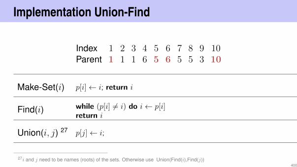
Implementation Union-Find
Index 1 2 3 4 5 6 7 8 9 10Parent 1 1 1 6 5 6 5 5 3 10
Make-Set(i) p[i]← i; return i
Find(i) while (p[i] 6= i) do i← p[i]return i
Union(i, j) 27 p[j]← i;
27i and j need to be names (roots) of the sets. Otherwise use Union(Find(i),Find(j))400

Optimisation of the runtime for Find
Tree may degenerate. Example: Union(8, 7), Union(7, 6),Union(6, 5), ...
Index 1 2 3 4 5 6 7 8 ..Parent 1 1 2 3 4 5 6 7 ..
Worst-case running time of Find in Θ(n).
401

Optimisation of the runtime for Find
Idea: always append smaller tree to larger tree. Requires additionalsize information (array) g
Make-Set(i) p[i]← i; g[i]← 1; return i
Union(i, j)if g[j] > g[i] then swap(i, j)p[j]← iif g[i] = g[j] then g[i]← g[i] + 1
⇒ Tree depth (and worst-case running time for Find) in Θ(log n)
402

[Observation]
TheoremThe method above (union by size) preserves the following propertyof the trees: a tree of height h has at least 2h nodes.
Immediate consequence: runtime Find = O(log n).
(not shown in class) 403

[Proof]
Induction: by assumption, sub-trees have atleast 2hi nodes. WLOG: h2 ≤ h1
h2 < h1:
h(T1 ⊕ T2) = h1 ⇒ g(T1 ⊕ T2) ≥ 2h
h2 = h1:
g(T1) ≥ g(T2) ≥ 2h2
⇒g(T1 ⊕ T2) = g(T1) + g(T2) ≥ 2 · 2h2 = 2h(T1⊕T2)
T1
T2
h1
h2
(not shown in class) 404

Further improvement
Link all nodes to the root when Find is called.
Find(i):j ← iwhile (p[i] 6= i) do i← p[i]while (j 6= i) do
t← jj ← p[j]p[t]← i
return i
Cost: amortised nearly constant (inverse of theAckermann-function).28
28We do not go into details here.405

Running time of Kruskal’s Algorithm
Sorting of the edges: Θ(|E| log |E|) = Θ(|E| log |V |). 29
Initialisation of the Union-Find data structure Θ(|V |)|E|× Union(Find(x),Find(y)): O(|E| log |E|) = O(|E| log |V |).
Overal Θ(|E| log |V |).
29because G is connected: |V | ≤ |E| ≤ |V |2406

Algorithm of Jarnik (1930), Prim, Dijkstra (1959)
Idea: start with some v ∈ V and grow the spanning tree from hereby the acceptance rule.
A← ∅S ← v0for i← 1 to |V | do
Choose cheapest (u, v) mit u ∈ S, v 6∈ SA← A ∪ (u, v)S ← S ∪ v // (Coloring)
S
V \ S
Remark: a union-Find data structure is not required. It suffices tocolor nodes when they are added to S.
407

Running time
Trivially O(|V | · |E|).Improvement (like with Dijkstra’s ShortestPath)
With Min-Heap: costs
Initialization (node coloring) O(|V |)|V |× ExtractMin = O(|V | log |V |),|E|× Insert or DecreaseKey: O(|E| log |V |),
O(|E| · log |V |)
408

16. Flow in Networks
Flow Network, Maximal Flow, Cut, Rest Network, Max-flow Min-cutTheorem, Ford-Fulkerson Method, Edmonds-Karp Algorithm,Maximal Bipartite Matching [Ottman/Widmayer, Kap. 9.7, 9.8.1],[Cormen et al, Kap. 26.1-26.3]
409

Motivation
Modelling flow of fluents, components on conveyors, current inelectrical networks or information flow in communication networks.Connectivity of Communication Networks, Bipartite Matching,Circulation, Scheduling, Image Segmentation, BaseballEliminination...
410

Flow Network
Flow network G = (V,E, c): directedgraph with capacitiesAntiparallel edges forbidden:(u, v) ∈ E ⇒ (v, u) 6∈ E.Model a missing edge (u, v) byc(u, v) = 0.Source s and sink t: special nodes.Every node v is on a path between sand t : s v t
s
v1
v2
v3
v4
t
16
13
12
14
20
4
94 7
411

FlowA Flow f : V ×V → R fulfills the followingconditions:
Bounded Capacity:For all u, v ∈ V : f(u, v) ≤ c(u, v).Skew Symmetry:For all u, v ∈ V : f(u, v) = −f(v, u).Conservation of flow:For all u ∈ V \ s, t:∑
v∈V
f(u, v) = 0.
s
v1
v2
v3
v4
t
16/8
13/10
12/12
14/10
20/14
4/4
9/44/4 7/6
Value of the flow:|f | =
∑v∈V f(s, v).
Here |f | = 18.
412

How large can a flow possibly be?
Limiting factors: cuts
cut separating s from t: Partition of V into S and T with s ∈ S,t ∈ T .Capacity of a cut: c(S, T ) =
∑v∈S,v′∈T c(v, v
′)
Minimal cut: cut with minimal capacity.Flow over the cut: f(S, T ) =
∑v∈S,v′∈T f(v, v′)
413

Implicit SummationNotation: Let U,U ′ ⊆ V
f(U,U ′) :=∑u∈Uu′∈U ′
f(u, u′), f(u, U ′) := f(u, U ′)
Thus
|f | = f(s, V )
f(U,U) = 0
f(U,U ′) = −f(U ′, U)
f(X ∪ Y, Z) = f(X,Z) + f(Y, Z), if X ∩ Y = ∅.f(R, V ) = 0 if R ∩ s, t = ∅. [flow conversation!]
414

How large can a flow possibly be?For each flow and each cut it holds that f(S, T ) = |f |:
f(S, T ) = f(S, V )− f(S, S)︸ ︷︷ ︸0
= f(S, V )
= f(s, V ) + f(S − s︸ ︷︷ ︸63t,63s
, V ) = |f |.
s
v1
v2
v3
v4
t
16/8
13/10
12/12
14/10
20/14
4/4
9/44/4 7/6
415

Maximal Flow ?In particular, for each cut (S, T ) of V .
|f | ≤∑
v∈S,v′∈T
c(v, v′) = c(S, T )
Will discover that equality holds for minS,T c(S, T ).
s
v1
v2
v3
v4
t
16
13
12
14
20
4
94 7
c = 23416

Maximal Flow ?
Naive Procedure
s
v1
v2
v3
v4
t
16/8
13/10
12/12
14/10
20/14
4/4
9/44/4 7/6 s
v1
v2
v3
v4
t
16/8
13/11
12/12
14/11
20/15
4/4
9/44/4 7/7
s
v1
v2
v3
v4
t
16/8
13/13
12/12
14/11
20/17
4/4
9/24/4 7/7 s
v1
v2
v3
v4
t
16/10
13/13
12/12
14/11
20/19
4/4
9/04/2 7/7
Conclusion: greedy increase of flow does not solve the problem.
417

The Method of Ford-FulkersonStart with f(u, v) = 0 for all u, v ∈ VDetermine rest network* Gf and expansion path in Gf
Increase flow via expansion path*Repeat until no expansion path available.
Gf := (V,Ef , cf)
cf(u, v) := c(u, v)− f(u, v) ∀u, v ∈ VEf := (u, v) ∈ V × V |cf(u, v) > 0
*Will now be explained418

Increase of flow, negative!
Let some flow f in the network be given.
Finding:
Increase of the flow along some edge possible, when flow can beincreased along the edge,i.e. if f(u, v) < c(u, v).Rest capacity cf(u, v) = c(u, v)− f(u, v) > 0.Increase of flow against the direction of the edge possible, if flowcan be reduced along the edge, i.e. if f(u, v) > 0.Rest capacity cf(v, u) = f(u, v) > 0.
419

Rest Network
Rest network Gf provided by the edges with positive rest capacity:
s
v1
v2
v3
v4
t
16/8
13/10
12/12
14/10
20/14
4/4
9/44/4 7/6
s
v1
v2
v3
v4
t8
8
3
10
12
4
10
6
14
4
5
4
4 1 6
Rest networks provide the same kind of properties as flow networks with the exception of permitting antiparallel
capacity-edges
420

Observation
TheoremLet G = (V,E, c) be a flow network with source s and sink t and f aflow in G. Let Gf be the corresponding rest networks and let f ′ be aflow in Gf . Then f ⊕ f ′ with
(f ⊕ f ′)(u, v) = f(u, v) + f ′(u, v)
defines a flow in G with value |f |+ |f ′|.
421

Prooff ⊕ f ′ defines a flow in G:
capacity limit
(f ⊕ f ′)(u, v) = f(u, v) + f ′(u, v)︸ ︷︷ ︸≤c(u,v)−f(u,v)
≤ c(u, v)
skew symmetry
(f ⊕ f ′)(u, v) = −f(v, u) +−f ′(v, u) = −(f ⊕ f ′)(v, u)
flow conservation u ∈ V − s, t:∑v∈V
(f ⊕ f ′)(u, v) =∑v∈V
f(u, v) +∑v∈V
f ′(u, v) = 0
422

Proof
Value of f ⊕ f ′
|f ⊕ f ′| = (f ⊕ f ′)(s, V )
=∑u∈V
f(s, u) + f ′(s, u)
= f(s, V ) + f ′(s, V )
= |f |+ |f ′|
423

Augmenting Paths
expansion path p: simple path from s to t in the rest network Gf .
Rest capacity cf(p) = mincf(u, v) : (u, v) edge in p
424

Flow in Gf
TheoremThe mapping fp : V × V → R,
fp(u, v) =
cf(p) if (u, v) edge in p−cf(p) if (v, u) edge in p0 otherwise
provides a flow in Gf with value |fp| = cf(p) > 0.
fp is a flow (easy to show). there is one and only one u ∈ V with(s, u) ∈ p. Thus |fp| =
∑v∈V fp(s, v) = fp(s, u) = cf(p).
425

Consequence
Strategy for an algorithm:
With an expansion path p in Gf the flow f ⊕ fp defines a new flowwith value |f ⊕ fp| = |f |+ |fp| > |f |.
426

Max-Flow Min-Cut Theorem
TheoremLet f be a flow in a flow network G = (V,E, c) with source s andsink t. The following statementsa are equivalent:
1 f is a maximal flow in G2 The rest network Gf does not provide any expansion paths3 It holds that |f | = c(S, T ) for a cut (S, T ) of G.
427
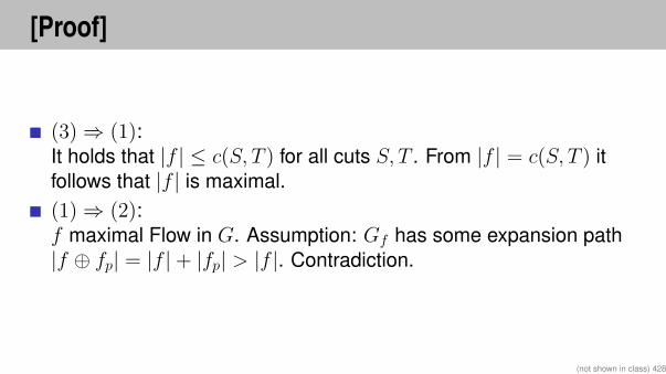
[Proof]
(3)⇒ (1):It holds that |f | ≤ c(S, T ) for all cuts S, T . From |f | = c(S, T ) itfollows that |f | is maximal.(1)⇒ (2):f maximal Flow in G. Assumption: Gf has some expansion path|f ⊕ fp| = |f |+ |fp| > |f |. Contradiction.
(not shown in class) 428

[Proof (2)⇒ (3)]Assumption: Gf has no expansion path
Define S = v ∈ V : there is a path s v in Gf.(S, T ) := (S, V \ S) is a cut: s ∈ S, t ∈ T .
Let u ∈ S and v ∈ T . Then cf(u, v) = 0, alsocf(u, v) = c(u, v)− f(u, v) = 0. Somit f(u, v) = c(u, v).
Thus
|f | = f(S, T ) =∑u∈S
∑v∈T
f(u, v) =∑u∈S
∑v∈T
c(u, v) = C(S, T ).
(not shown in class) 429

Algorithm Ford-Fulkerson(G, s, t)
Input: Flow network G = (V,E, c)Output: Maximal flow f .
for (u, v) ∈ E dof(u, v)← 0
while Exists path p : s t in rest network Gf docf (p)← mincf (u, v) : (u, v) ∈ pforeach (u, v) ∈ p do
f(u, v)← f(u, v) + cf (p)f(v, u)← f(v, u)− cf (p)
430

Practical Consideration
In an implementation of the Ford-Fulkerson algorithm the negativeflow egdes are usually not stored because their value always equalsthe negated value of the antiparallel edge.
f(u, v)← f(u, v) + cf (p)f(v, u)← f(v, u)− cf (p)
is then transformed toif (u, v) ∈ E then
f(u, v)← f(u, v) + cf (p)else
f(v, u)← f(v, u)− cf (p)
431

Analysis
The Ford-Fulkerson algorithm does notnecessarily have to converge for irrationalcapacities. For integers or rational numbers itterminates.For an integer flow, the algorithms requiresmaximally |fmax| iterations of the while loop(because the flow increases minimally by 1).Search a single increasing path (e.g. withDFS or BFS) O(|E|) Therefore O(fmax|E|).
s
u
v
t
1000
1000
1
1000
1000
With an unlucky choice the al-gorithm may require up to 2000iterations here.
432

Edmonds-Karp Algorithm
Choose in the Ford-Fulkerson-Method for finding a path in Gf theexpansion path of shortest possible length (e.g. with BFS)
433

Edmonds-Karp Algorithm
TheoremWhen the Edmonds-Karp algorithm is applied to some integervalued flow network G = (V,E) with source s and sink t then thenumber of flow increases applied by the algorithm is in O(|V | · |E|).⇒ Overal asymptotic runtime: O(|V | · |E|2)
[Without proof]
434

Application: maximal bipartite matchingGiven: bipartite undirected graph G = (V,E).
Matching M : M ⊆ E such that |m ∈M : v ∈ m| ≤ 1 for all v ∈ V .
Maximal Matching M : Matching M , such that |M | ≥ |M ′| for eachmatching M ′.
435

Corresponding flow networkConstruct a flow network that corresponds to the partition L,R of abipartite graph with source s and sink t, with directed edges from sto L, from L to R and from R to t. Each edge has capacity 1.
L R
s t
L R
436

[Integer number theorem]
TheoremIf the capacities of a flow network are integers, then the maximalflow generated by the Ford-Fulkerson method provides integernumbers for each f(u, v), u, v ∈ V .
[without proof]
Consequence: Ford-Fulkerson generates for a flow network thatcorresponds to a bipartite graph a maximal matchingM = (u, v) : f(u, v) = 1.
(not shown in class) 437