Embed Size (px)
Citation preview

Computer Science & Information Technology 68


David C. Wyld Natarajan Meghanathan (Eds)
Computer Science & Information Technology
Seventh International Conference on Computer Science, Engineering and Information Technology (CCSEIT 2017) Vienna, Austria, May 27~28, 2017
AIRCC Publishing Corporation

Volume Editors
David C. Wyld, Southeastern Louisiana University, USA E-mail: [email protected] Natarajan Meghanathan, Jackson State University, USA E-mail: [email protected] ISSN: 2231 - 5403 ISBN: 978-1-921987-66-3
DOI : 10.5121/csit.2017.70601 - 10.5121/csit.2017.70613
This work is subject to copyright. All rights are reserved, whether whole or part of the material is concerned, specifically the rights of translation, reprinting, re-use of illustrations, recitation, broadcasting, reproduction on microfilms or in any other way, and storage in data banks. Duplication of this publication or parts thereof is permitted only under the provisions of the International Copyright Law and permission for use must always be obtained from Academy & Industry Research Collaboration Center. Violations are liable to prosecution under the International Copyright Law. Typesetting: Camera-ready by author, data conversion by NnN Net Solutions Private Ltd., Chennai, India

Preface
The Seventh International Conference on Computer Science, Engineering and Information Technology (CCSEIT 2017) was held in Vienna, Austria, during May 27~28, 2017. The Fourth International Conference on Artificial Intelligence and Applications (AIAP 2017), The Fourth International Conference on Data Mining and Database (DMDB 2017), The Fourth International Conference on Bioinformatics and Bioscience (ICBB 2017) and The Tenth International Conference on Security and its Applications (CNSA 2017) was collocated with the Seventh International Conference on Computer Science, Engineering and Information Technology (CCSEIT 2017). The conferences attracted many local and international delegates, presenting a balanced mixture of intellect from the East and from the West. The goal of this conference series is to bring together researchers and practitioners from academia and industry to focus on understanding computer science and information technology and to establish new collaborations in these areas. Authors are invited to contribute to the conference by submitting articles that illustrate research results, projects, survey work and industrial experiences describing significant advances in all areas of computer science and information technology. The CCSEIT-2017, AIAP-2017, DMDB-2017, ICBB-2017, CNSA-2017 Committees rigorously invited submissions for many months from researchers, scientists, engineers, students and practitioners related to the relevant themes and tracks of the workshop. This effort guaranteed submissions from an unparalleled number of internationally recognized top-level researchers. All the submissions underwent a strenuous peer review process which comprised expert reviewers. These reviewers were selected from a talented pool of Technical Committee members and external reviewers on the basis of their expertise. The papers were then reviewed based on their contributions, technical content, originality and clarity. The entire process, which includes the submission, review and acceptance processes, was done electronically. All these efforts undertaken by the Organizing and Technical Committees led to an exciting, rich and a high quality technical conference program, which featured high-impact presentations for all attendees to enjoy, appreciate and expand their expertise in the latest developments in computer network and communications research. In closing, CCSEIT-2017, AIAP-2017, DMDB-2017, ICBB-2017, CNSA-2017 brought together researchers, scientists, engineers, students and practitioners to exchange and share their experiences, new ideas and research results in all aspects of the main workshop themes and tracks, and to discuss the practical challenges encountered and the solutions adopted. The book is organized as a collection of papers from the CCSEIT-2017, AIAP-2017, DMDB-2017, ICBB-2017, CNSA-2017. We would like to thank the General and Program Chairs, organization staff, the members of the Technical Program Committees and external reviewers for their excellent and tireless work. We sincerely wish that all attendees benefited scientifically from the conference and wish them every success in their research. It is the humble wish of the conference organizers that the professional dialogue among the researchers, scientists, engineers, students and educators continues beyond the event and that the friendships and collaborations forged will linger and prosper for many years to come.
David C. Wyld Natarajan Meghanathan

Organization
General Chair
Natarajan Meghanathan, Jackson State University, USA Brajesh Kumar Kaushik, Indian Institute of Technology - Roorkee, India Program Committee Members
Abdolreza hatamlou Islamic Azad University, Iran Adnan Rawashdeh Yarmouk University, Jordan Ahmed Hussein Aliwy University of Kufa, Iraq Ahmed Korichi University of Ouargla, Algeria Ahmed Mohamed Khedr Sharjah university, UAE Alborzi Nanyang Technological University, Singapore Aleksandar Sugaris ICT College , Serbia Ali Hakan Eastern Mediterranean University, North Cyprus Amirrudin Kamsin University of Malaya, Malaysia Atallah M, AL-Shatnawi Al al-Byte University, Jordan Azeddine Chikh University of Tlemcen, Algeria Belal M. Abuata Yarmouk University, Jordan Chandran Somasundram University of Malaya, Malaysia Dabin Ding University of Central Missouri, United States Doina Bein The Pennsylvania State University, USA Elaheh Pourabbas National Research Council, Italy Emad Awada Applied Science University, Jordan Emilio Jimenez Macias University of La Rioja, Spain Erritali Mohammed Sultan Moulay Slimane University, Morocco Eyad M. Hassan ALazam Yarmouk University,Jordan Farnaz Lorestani University Malaya, Malaysia Fei Deng University of California, USA Fernando Tello Gamarra Federal University of Santa Maria, Brazil Gammoudi Aymen University of Tunis, Tunisia Hamed Al-Rubaiee University of Bedfordshire,United Kingdom Hamid Abdullah Jalab University of Malaya, Malaysia Hamid Alasadi Basra University, Iraq Hayet Mouss Batna Univeristy, Algeria Hèldon Josè Integrated Faculties of Patos, Brazil Hongzhi Harbin Institute of Technology, China Houcine Hassan Univeridad Politecnica de Valencia, Spain Ivan Popovic University of Belgrade, Serbia Ilham Huseyinov Istanbul Aydin University, Turkey Jae Kwang Lee Hannam University, South Korea Jamal El Abbadi Mohammadia V University Rabat, Morocco John Tass University of Patras, Greece Jun Zhang South China University of Technology, China

Kayhan Erciyes Izmir University, Turkey Kheireddine abainia USTHB university, Algeria Kishore Rajagopalan Prairie Research Institute, US Lee Beng Yong Universiti Teknologi MARA, Malaysia Liyakathunisa Syed Prince Sultan University, Saudi Arabia Luigi Nicolais Emeritus Professor University of Naples, Italy Mahdi Mazinani IAU Shahreqods, Iran Mahdi Salarian University of Illinois, USA Malik Mubashir Hassan Directorate of IT & Communication, France Masoumeh Javanbakht Hakim Sabzevari University,Iran Maysaa El Sayed Zaki Clinical Pathology, Egypt Miguel Ángel Giráldez Sánchez Hospital Virgen del Rocío, Spain Mohamed Abouleish American University of Sharjah, UAE Mohamed AMROUNE Larbi Tebessi university, Algeria Mohamed Elhoseny Mansoura University, Egypt Mohamedmaher Benismail King Saud University, Saudi Arabia Mohammad alsarem Taibah University, KSA Mohammad Rawashdeh University of Central Missouri, United States Mohammed A. Awadallah Al-Aqsa University, Palestine Mohammed AbouBakr Elashiri Beni Suef University, Egypt Mohammed Ghazi Al-Zamel Yarmouk University,Jordan Mostafa Ashry Alexandria University, Egypt Mourchid mohammed Ibn Tofail University Kenitra, Morocco Nahlah Shatnawi Yarmouk University, Jordan Necmettin Erbakan University, Turkey Nesrene Omar Mansoura University, Egypt Nicolas H. Younan Mississippi State University, USA Nor Liyana Mohd Shuib University of Malaya, Malaysia Noura Taleb Badji Mokhtar University, Algeria Ouafa Mah Ouargla university, Algeria P. K. Paul Raiganj University, India Parvaneh. Shams İstanbul Aydın University, Iran Razieh malekhoseini Islamic Azad University, Iran Sajad Einy Sakarya University, Turkey Soumaya Chaffar Prince Sultan University, Saudi Arabia Sunil Vadera University of Salford, UK Supawan Tirawanichakul Prince of Songkla University, Thailand Syazwani Itri Amran Universiti Teknologi Malaysia (UTM), Malaysia Taeghyun Kang University of Central Missouri, United States Tse Guan Tan Universiti Malaysia Kelantan, Malaysia Vahid Khalilzad-Sharghi Medical Imaging Solutions, GA USA Walace Gomes Leal Federal University of Pará-Belém, Brazil Wonjun Lee The University of Texas at San Antonio, USA Xuechao Li Auburn University, USA Yutthana Tirawanichakul Prince of Songkla University, Thailand Zati Hakim Azizul Hasan University of Malaya, Malaysia

Technically Sponsored by
Computer Science & Information Technology Community (CSITC)
Networks & Communications Community (NCC)
Database Management Systems Community (DBMSC)
Organized By
Academy & Industry Research Collaboration Center (AIRCC)

TABLE OF CONTENTS
Seventh International Conference on Computer Science, Engineering
and Information Technology (CCSEIT 2017)
A Few Thoughts on Code Review and Cooperative Pair Programming :
Expectations, Outcomes and Challenges ……………………………...….…....... 01 - 07
Qiang Fu, Francis Grady, Bjoern Flemming Broberg, Andrew Roberts,
Geir Gil Martens, Kjetil Vatland Johansen and Pieyre Le Loher
Fault Tolerant Consensus Agreement Algorithm………….………………........ 09 - 14
Marius Rafailescu
Evaluation of Scalable PRPL Schemes with a Native LSH Database
Engine………………………………………………...…….………………........ 125 - 132
Dimitrios Karapiperis, Chris T. Panagiotakopoulos and Vassilios S. Verykios
Fourth International Conference on Artificial Intelligence and
Applications (AIAP 2017)
Music Mood Dataset Creation Based on Last FM Tags………………….…...... 15 - 26
Erion Çano and Maurizio Morisio
Effective Vector Representations for Variable Length Symbol Sequences….... 27 - 34
Gustavo Lado and Enrique Carlos Segura
Clustering for Different Scales of Measurement - The Gap Ratio Weighted
K-Means Algorithm……………………………...………………………....…....... 35 - 52
Joris Guerin, Olivier Gibaru, Stephane Thiery and Eric Nyiri
A Self-Organizing Recurrent Neural Network Based on Dynamic Analysis.…. 53 - 66
Qili Chen, Junfei Qiao and Yi Ming Zou
Fourth International Conference on Data Mining and Database
(DMDB 2017)
Holistic Approach to Predicting Students Performance in Higher Educational
Institutions - A Conceptual Framework………………….…………………........ 67 - 74
Olugbenga Adejo and Thomas Connolly

A Model of Extracting Patterns in Social Network Data Using Topic
Modelling, Sentiment Analysis and Graph Databases……………..………….... 75 - 84
Assane Wade and Giovanna Di MarzoSerugendo
Mutual Information to Interpret the Semantics of Anomalies in Link
Mining……………………………………………………..………..………….... 113 - 123
Zakea Il-agure and Belsam Attallah
Fourth International Conference on Bioinformatics and Bioscience
(ICBB 2017)
Fingerprint Recognition Algorithm………………….………….…………........ 85 - 100
Farah Dhib Tatar
Thermal Imaging Using CNN and KNN Classifiers with FWT, PCA and
LDA Algorithms………………….………….………………………………...... 133 - 143
Chigozie Orji , Evan Hurwitz and Ali Hasan
Tenth International Conference on Security and its Applications
(CNSA 2017)
Improvement of Email Threats Detection by User Training……………........ 101 - 111
V.Bernard, P-Y.Cousin, A.Lefaillet, M.Mugaruka and C.Raibaud

David C. Wyld et al. (Eds) : CCSEIT, AIAP, DMDB, ICBB, CNSA - 2017
pp. 01– 07, 2017. © CS & IT-CSCP 2017 DOI : 10.5121/csit.2017.70601
A FEW THOUGHTS ON CODE REVIEW AND
COOPERATIVE PAIR PROGRAMMING :
EXPECTATIONS, OUTCOMES AND
CHALLENGES
Qiang Fu, Francis Grady, Bjoern Flemming Broberg, Andrew Roberts,
Geir Gil Martens, Kjetil Vatland Johansen, Pieyre Le Loher
Schlumberger Information Solutions AS, Stavanger, Norway
ABSTRACT
The paper discusses the about the improvement of mandatory code review and pair
programming practiced in the commercial software development, and also proposes effective
approaches to customize the code review and pair programming to avoid the pitfalls and keep
the benefits.
KEYWORDS
Code review, pair programming
1. INTRODUCTION
Code review, a manual inspection of source code by developers other than the author, is a
common software engineering practice employed in industrial contexts and is recognized as a
valuable tool for reducing defects and improving quality. The policy of 100 percent code review
has been implemented / discussed in many commercial software projects.
Classical pair programming is an agile software development technique in which two
programmers work together at one workstation [1]. Traditionally, one programmer writes code
while the other reviews each line of code as it is typed in. The two programmers switch roles
frequently. Some obvious benefits can be achieved with pair programming: 1) fewer bugs, 2)
lower cost on production maintenance, and 3) knowledge transfer [2, 3]. Another benefit is that
both developers acquire a good understanding of all the written code; they know what the design
choices were and how the code works. From many aspects, this reduces the fragmentation of
knowledge within a team.
Another agile software development technique, pair programming is also becoming increasingly
popular in the software industry. It is commonly considered that pair programming can get more
maintainable design with better quality, but in real working environment it often trapped in some
pitfalls [4,5]:

2 Computer Science & Information Technology (CS & IT)
1) Discourages introversion. The coder must “program aloud” while the reviewer listens.
Some developers will not raise concerns or suggest corner cases, thus turning the pair
programming into “solitary programming” with automatic code review, which wastes
resources.
2) Prevents creativity. Contrary to the value of “group brainstorming”, creative work
sometimes requires independence and autonomy. In pair programming, developers must
be able to convince a partner of the merits of an idea. This requires talking through the
implementation
3) Step by step and risking being judged if the idea fails.
4) Tiring practice. A good pair programming session is intense and mentally demanding.
Programmers have reported significant exhaustion after just a few hours. This is a
common observation, even from the most experienced practitioners and the advocates of
pair programming.
5) Demanding balance maintenance. Pair programming can cost more work-hours than
solitary programming to produce the same feature if the cooperation is not planned
properly. A balance must be maintained carefully between the quality of code and the
increased programming cost.
Mandatory code review and pair programming are being practiced in our team recently. Based on
the actual circumstance of our team, the traditional code review and pair programming are
tailored to get the advantages and avoid the pitfalls mentioned above.
2. CODE REVIEW
Mandatory code review was introduced in our team in July 2016. Although our main motivation
for conducting code reviews was finding bugs, we found that reviews brought several additional
benefits including knowledge transfer, increased team awareness and the creation of more elegant
solutions.
Many code review guidelines recommend that the original author of a piece of code perform the
review of any subsequent changes; in our case, that is largely impossible. Team and code
ownership changes mean that the original author may work in a different team by the time the
code is reviewed. Instead, we have introduced a simple rota for performing reviews. Every week,
one developer is “on duty” for reviewing changes from all other developers.
To help improve review consistency, we have agreed on a checklist for both the author and the
reviewer to follow (Figure 1), and two reviewers are required when new team members join the
team. This enables us to verify that key code goals such as readability, maintainability, and
functionality are met.

Computer Science & Information Technology (CS & IT) 3
Figure 1 Customized code review checklist
Since one of the potential issues with code reviews is the lag time that they introduce into the
development cycle, we added informal requirements that the size of the code to be reviewed be
kept small and that reviews are completed in under 1 hour.
The overview of the code reviews can be setup in the Team Foundation Server (TFS) dashboard
(Figure 2).
3. COOPERATIVE PAIR PROGRAMMING
The project on which we tried cooperative pair programming was the creation of a new public
API. The requirements and acceptance criteria were relatively clear, so the implementation,
proper tests, and sample codes were the main work. Two developers worked on the project
together, and both had adequate understanding on the work, which reduced the amount of
discussion needed. Therefore, instead of having two people working on the same computer all
day and swapping roles frequently, we tailored our usage as follows:
1. As with classical pair programming, we sit together and agree on the API details such as
the names, parameters, constants, etc.
2. After the API details are decided, the developerswork at separate computers. One person
works on the API implementation, and the other works on the tests for the designed API.
3. At the end of each day, regardless of whether the implementation or tests were finished,
the developers swap roles. The person who was working on the API implementation
reviews the test code and continues the test implementation, and vice-versa.
4. Steps 2 and 3 are then repeated until the work is complete.

4 Computer Science & Information Technology (CS & IT)
By following this cooperative pair programming model, we gained several advantages:
1. We performed detailed and in-depth code reviews, which led to fewer bugs. Unlike
common code reviews, we developed a stronger understanding of the code and the
frequent communication that was required made it easier to find some of the more
obscure bugs.
2. We observed a clear improvement in the quality of the code, including better readability
and less unnecessary and unused code.
3. By switching the roles, API implementation code and its test code received a more
thorough review.
4. We perceived increased knowledge sharing because it was necessary to understand the
code thoroughly to continue the work. Because the code was fresh in the one developer’s
mind, it was easier to explain the intent to the other developer in the pair.
5. Both developers retained autonomy and the ability to exercise creativity. Both were free
to try an approach before having to convince the other developer.
6. We obtained 100%code coverage. Both developers spent the same amount of time
writing the unit/acceptance tests as writing the API implementation.
Figure 2 Code review in TFS dashboard

Computer Science & Information Technology (CS & IT) 5
4. EXPECTATIONS AND OUTCOMES
After 4 months of mandatory code review, we have discovered that finding defects is not the only
benefit of code review. Reinforced by a strong team culture around the reviews, we see several
benefits:
Code quality improvements: A clear improvement on the code quality can be observed because of
the mandatory review. Improvements include better unit testing, fewer unnecessary changes and
improved readability.
Defect finding: The detailed checklist and improved code quality enable us to discoverobvious
bugs such as exception handling, raw pointer misuser, typos and formatting mistakes. There was
a gap between our expectations and reality in terms of the types of defects found. However, we
still derive a benefit from catchingthe more obvious bugs earlier than in conventional
programming.
Knowledge transfer: The team works on multiple separate projects. Code reviews help facilitate
knowledge transfer between team members, not only helping to expose reviewers to a wider
range of code, but also directing authors to other resources for learning how to solve some
problems.
Team awareness and transparency: By performing mandatory code reviews, we not only keep the
team generally aware of changes in the code, we also prevent anyone from adding low quality
“Band-Aid” fixes to the code in secret.
From our cooperative pair programming experiment, we have discovered some conditions that
effect the success of pair programming:
1) The maturity of the design
2) The comparative skill levels of the developers involved
3) The scale of the work, with the best scale being a task totalling at least two person-
months estimated work.
5. RECOMMENDATIONS
From our experience with code reviews and pair programming, we can offer several observations
and recommendations:
Customized checklist: Each team should have tailored checklist according to its programming
environment and team culture, and this checklist should be updated as the team and its projects
change.
Quality assurance: Code reviews rarely result in identifying subtle bugs, so standard QA
practices such as automated unit testing and acceptance tests should be maintained.

6 Computer Science & Information Technology (CS & IT)
Beyond defects: Code reviews provide benefits beyond finding defects. They can be used to help
standardize style, find alternative solutions and increase learning. These goals should guide code
review policies.
Customized pair programming: Cooperative pair programming is just one of many possible
customizations of pair programming. Depending on the circumstances, different variants of pair
programming could be tried to provide an optimal balance between quality and cost.
REFERENCES
[1] Fagan, M.E., (1976) Design and Code inspections to reduce errors in program development, IBM
Systems Journal, Vol. 15, No 3, pp. 182-211
[2] Shore, James, (2007) The art of agile development, O’Reilly Media, Inc.
[3] Cockburn, Alistair, (2002) Agile software development. Vol. 2006. Boston: Addison-Wesley.
[4] http://www.bennorthrop.com/Essays/2013/pair-programming-my-personal-nightmare.php
[5] https://techcrunch.com/2012/03/03/pair-programming-considered-harmful/
[6] Holzmann, G.J., (2006) The Power of Ten: Rules for developing safety critical code, IEEE Computer.
[7] Russell, G. W. (1991) Experience with Inspection in Ultralarge-Scale Developments, IEEE , pp. 25-
31.
[8] Beller, M; Bacchelli, A; Zaidman, A; Juergens, E (2014), Modern code reviews in open-source
projects: which problems do they fix?, Proceedings of the 11th Working Conference on Mining
Software Repositories
[9] Bisant, David B, (1989) A Two-Person Inspection Method to Improve Programming Productivity,
IEEE Transactions on Software Engineering. 15 (10), pp.1294–1304.
AUTHORS
Qiang Fu was born in China in 1977. He received the Ph.D degree from Imperial
College London in 2010. He joined Schlumberger Information Solution AS in 2011 as
senior software developer in Petrel Geophysics team. His main areas of research
interest are software processing, developing, geophysics and geology.
Francis Grady received his Master’s degree in Computer Science from the University
of Oxford in 2006. Since then he has been with Schlumberger, where he is currently a
Senior Software Engineer. His interests include machine learning, high performance
computing and code quality.

Computer Science & Information Technology (CS & IT) 7
Bjoern Flemming Broberg joined Schlumberger in 2013 working as a Senior
Software Engineer developing software. He has a master in industrial mathematics
from Trondheim in Norway, and has more than 20 years of experience as an IT
professional working as business analyst, IT architect, developer and IT project
manager.
Andrew Roberts has worked for six years at Sclumberger as a Software Engineer, in
development, build and configuration management, and testing roles. Prior to
Sclumberger he was Software Consultant for over a decade in the mobile devices
market working with such companies as Motorola, Nokia, Panasonic, etc.
Geir Gil Martens was born in Bergen, Norway, 1960. After acquiring an
undergraduate degree in computer science at Rogaland Distriktshøgskule, Norway. He
joined Geophysical Company of Norway – GECO AS in 1985 to develop the Charisma
II Seismic Interpretation Station. Over the years he have been involved with most
aspects of software development and a multitude of more or less formalized
development processes. He is currently working at Schlumberger SNTC as a senior
software engineer on the Petrel system.
Kjetil Vatland Johansen has a M.Sc. degree in Technical Cybernetics from
Norwegian University of Science and Technology. He has combined background from
cybernetics with a passion for software development throughout the professional career.
He was a developer in an C++/.Net environment for 15 years and then moved to project
management.

8 Computer Science & Information Technology (CS & IT)
INTENTIONAL BLANK

David C. Wyld et al. (Eds) : CCSEIT, AIAP, DMDB, ICBB, CNSA - 2017
pp. 09– 14, 2017. © CS & IT-CSCP 2017 DOI : 10.5121/csit.2017.70602
FAULT TOLERANT CONSENSUS
AGREEMENT ALGORITHM
Marius Rafailescu
The Faculty of Automatic Control and Computers,
POLITEHNICA University, Bucharest
ABSTRACT
Recently a new fault tolerant and simple mechanism was designed for solving commit consensus
problem. It is based on replicated validation of messages sent between transaction participants
and a special dispatcher validator manager node. This paper presents a correctness, safety
proofs and performance analysis of this algorithm.
KEYWORDS
consensus agreement, fault tolerance, leader election, distributed systems
1. INTRODUCTION
Consensus algorithms were discussed in the past and several solutions where developed (Two-
phase commit, Three-phase commit or Paxos) [1]. The latter is fault tolerant and with the
introduction of distributed databases it was implemented in many systems, although it is not so
easy to implement [2]. In recent years was defined a new algorithm, Raft, which has been
developed in order to provide a consensus control for replicated state machines, intended to be
easy to understand and implement [3].
One recent work [4] describes a new algorithm which uses a set of validator nodes, including one
dispatcher and also presents algorithm for dispatcher election (equivalent to leader election) made
for the purpose of not rollbacking the transaction when a new dispatcher is chosen. Based on this
new consensus agreement solution, this paper highlights the correctness and safety proofs of the
algorithm.
2. DESCRIPTION The system is modelled in an asynchronous way (with the corresponding implication of using
timeouts - as a well known result [5]), having the following suppositions:
• Messages can take an arbitrary number of steps from source to destination;
• Messages can be reordered, duplicated or lost by the network, but never corrupted;
• Nodes fail by stopping; later, they can restart and re-enter in the system.

10 Computer Science & Information Technology (CS & IT)
The specification describes a system with an arbitrary number of nodes, which communicate
through messages which are sent in two manners: one-to-one and one-to-many as we can see in
figure 1.
Fig. 1: Consensus messages
3. CORRECTNESS
Correctness is an important key concern when talking about consensus algorithms. The formal
specification for the proposed algorithm was made using TLA+ language [6].
The model verifies defined invariants in order to test that the algorithm is correct and, as a whole,
the specification is intended to serve as the subject of the proof. This also help other people to
implement easily and correctly the algorithm in real systems. There may be many causes for
failures and maybe some of them can not be tested, but the formal tool help us to analyze all the
final states a system can reach in order to identify and resolve potential problems.
3.1. CONSENSUS SPECIFICATION
All the actions a node may take are described below:
• Transaction manager is the node which initiate the transaction and his special role is to
send “Begin” message to all other transaction participants. It is also a participant in

Computer Science & Information Technology (CS & IT) 11
transaction, so all the actions below are applicable, except receiving “Begin” message
step;
• Participant nodes, chronologically are initially in a “working” state. As soon as they
receive the “Begin” message from the transaction manager, they move into “preparing”
state. During this step, the transaction is locally finalized and every such node ensures
that the transaction can be recovered in case of a failure. After all the processings have
been done, every participant sends one “Ready” message to dispatcher manager and
moves to “ready” state. In this state, each node waits for receiving the commit or rollback
decision from the dispatcher node;
• Dispatcher node coordinates all validator nodes which work together in order to ensure
fault tolerance in case of a dispatcher failure. The node receives “Ready” messages from
participants. As soon as such a message is received, it validates locally the message and
sends it to other validators. One message is considered validated when validator nodes
mark it in majority (in other words, this happens when the dispatcher manager have been
received sufficient “Validated” messages). After all the “Ready” messages of a
transaction are validated, this node has to send the “Commit” message to all transaction
participants. In the end, “Committed” message is sent to other validators in order to mark
that the transaction is finished. Of course, the “Rollback” message may be send when not
all the messages are validated;
• Validator nodes receive from the dispatcher node some “Ready” messages which are
first locally validated, then they send “Validated” message back to the dispatcher.
3.2. DISPATCHER ELECTION SPECIFICATION
Validating a message means, at least, saving into local memory that message or only the metadata
needed for dispatcher failover, which is done using an election algorithm:
• Coordinator node: Initially, all validator nodes try to satisfy the launch condition which
consist in generating three consecutive numbers greater than a chosen threshold. When
this happens, the node sends a “Proposal” message alongside with the greatest random
generated number. When the node is voted in majority, it becomes “coordinator” and runs
a roulette wheel selection algorithm using the numbers received from other nodes. The
winner of this selection will be the leader and its status will be announced to all nodes;
• Other nodes: When the “Proposal” message is received, the node votes for sender if it is
the first time in the current round of vote and sends his greatest random generated
number.
The new dispatcher needs to finalize all pending transactions and this may be a problem unless an
additional convention is used. There are some cases which must be analysed:
1) Old dispatcher fails after receiving a certain “Ready” message and sending at least one
validation message for that “Ready” message. One of the validators which received the
validation message will be elected as the new dispatcher. But the problem is that it does
not know anything about other “Ready” messages which might have been sent by other
participants and not sent for validation by the old dispatcher. One simple solution is that
every participant must send all pending “Ready” messages to the new dispatcher when
its announcement is made;

12 Computer Science & Information Technology (CS & IT)
2) Old dispatcher fails before sending to validation the first “Ready” message of a
transaction or before receiving the first “Ready” message of a transaction. Of course, the
new chosen dispatcher will not know anything about that transaction, so the previous
solution could also help in this case.
The conclusion is that there is necessary to add an additional step which consist in sending all
pending “Ready” messages from participants to the new dispatcher, when its announcement is
made. In this way those transactions can be committed. Initially, in [6], was mentioned an
eligibility constraint as only the validator nodes which received the last message sent by the old
dispatcher can be valid candidates for leader position; so, an important aspect which appears in
this context is that the constraint might be dropped.
4. ALGORITHM SAFETY PROOFS Definition 1. Each node’s current vote round monotonically increases.
This is straightforward from specification.
Definition 2. There is at most one coordinator in dispatcher election step.
Let’s consider there may be two coordinators for the same election round, C1 and C2. This case
can appear, of course, when a split vote is happening.
C1 and C2 received the majority of votes, then let M1 be the set of nodes which gave their votes for
C1 and M2 the set with all the nodes which voted for C2.
Let node V be V = M1 ∩ M2; this means that V voted for both C1 and C2 ⇒ based on specification,
this is impossible because V votes only for the first time in a round of vote, so
C1 = C2.
Definition 3. In the end of dispatcher election, only one new dispatcher is chosen.
This results directly from the previous proof as one coordinator will choose only one node as
dispatcher, from specification.
Definition 4. The algorithm chooses a dispatcher even nodes crash, where N is the
total number of validator nodes.
This results from specifications because the leader is chosen by coordinator node, which is
elected with the majority of votes from other nodes. If nodes crash, there is no
problem as majority can still be reached.
Definition 5. The algorithm commits a transaction even validator nodes crash.
This is similar with the previous proof as from specifications the transaction is committed when
all the “Ready” messages from participants are validated. One message is validated when
validator nodes approve it in majority, so the algorithm works fine even validator
nodes crash because majority can still be reached.
Definition 6. The algorithm commits transactions even the dispatcher fails while processing.
After the current dispatcher fails, a new one is elected and its first task will consist in interpreting
the messages it will receive from participant nodes and the pending transactions will continue the
commit consensus as previously mentioned. Based on the received list of “Ready” messages, the
new leader of validator nodes will know the status of each transaction in order to take all the

Computer Science & Information Technology (CS & IT) 13
necessary decisions (for example, send messages to validation or mark a transaction as
committed).
5. PERFORMANCE Performance test was made using 5 nodes running on distinct virtual machines and the consensus
for a transaction finished in 235 milliseconds in average, with a minimum of 140 milliseconds
and a maximum of 313 milliseconds. In 90% of cases, consensus was reached in at most 289
milliseconds.
More than 1000 concurrent transactions were taken into account. The histogram is shown in
figure 2.
Fig. 2: Consensus performance
6. CONCLUSION
The new algorithm analysed in this paper is quite simple and easy to understand. It is correct and
safe, proposing a method to solve the consensus agreement problem by using a set of nodes
which validate the messages sent between transaction participants and the leader of the validator
nodes, called dispatcher validator. It can recover in case this dispatcher node crash and has the
capability to continue the pending transactions and commit them eventually.
REFERENCES
[1] J. Gray & L. Lamport, (2006) “Consensum on transaction commit”, ACM Trans. Database Syst., Vol
31, No. 1, pp133-160.
[2] T. Chandra & R. Griesemer & J. Redstone, (2007) “Paxos made live - an engineering perspective”,
ACM Principles of distributed computing, pp398-407.
[3] D. Ongaro & J. Ousterhout, (2014) “In search of an understandable consensus algorithm (extended
version)”, Proceedings of the 2014 USENIX Conference on USENIX Annual Technical Conference,
pp305-320.

14 Computer Science & Information Technology (CS & IT)
[4] M. Rafailescu & M. S. Petrescu, (2017) “Fault tolerant consensus protocol for distributed database
transactions”, Proceedings of the 2017 International Conference on Management Engineering,
Software Engineering and Service Sciences, ICMSS ’17, pp90–93.
[5] M. J. Fischer & N. A. Lynch & M. S. Paterson, (1985) “Impossibility of distributed consensus with
one faulty process”, Journal of the Association for Computing Machinery, Vol. 32, No. 2, pp398-407.
[6] L. Lamport, (2002) “Specifying Systems: The TLA+ Language and Tools for Hardware and Software
Engineers”, Addison-Wesley Longman Publishing Co., Inc.
AUTHORS
Marius Rafailescu is a Ph.D. candidate at the Department of Computer Science at the “Politehnica”
University from Bucharest. His M.S. and B.S were received also from the “Politehnica” University from
Bucharest. His main research interests are transactional processing in databases and distributed systems

David C. Wyld et al. (Eds) : CCSEIT, AIAP, DMDB, ICBB, CNSA - 2017
pp. 15– 26, 2017. © CS & IT-CSCP 2017 DOI : 10.5121/csit.2017.70603
MUSIC MOOD DATASET CREATION BASED
ON LAST.FM TAGS
Erion Çano and Maurizio Morisio
Department of Control and Computer Engineering, Polytechnic University of
Turin, Duca degli Abruzzi, 24, 10129 Torino, Italy
ABSTRACT Music emotion recognition today is based on techniques that require high quality and large
emotionally labeled sets of songs to train algorithms. Manual and professional annotations of
songs are costly and hardly accomplished. There is a high need for datasets that are public,
highly polarized, large in size and following popular emotion representation models. In this
paper we present the steps we followed to create two such datasets using intelligence of last.fm
community tags. In the first dataset, songs are categorized based on an emotion space of four
clusters we adopted from literature observations. The second dataset discriminates between
positive and negative songs only. We also observed that last.fm mood tags are biased towards
positive emotions. This imbalance of tags was reflected in cluster sizes of the resulting datasets
we obtained; they contain more positive songs than negative ones.
KEYWORDS Music Sentiment Analysis, Ground-truth Dataset, User Affect Tags, Semantic Mood Spaces
1. INTRODUCTION
Music sentiment analysis or music mood recognition has to do with utilizing machine learning,
data mining and other techniques to classify songs in 2 (pos vs. neg) or more emotion categories
with highest possible accuracy. Several types of features such as audio, lyrics or metadata can be
used or combined together. Recently there is high attention on corpus-based methods that involve
machine or deep learning techniques [1]. There are studies that successfully predict music
emotions based on lyrics features only [2, 3, 4] utilizing complex models. Large datasets of songs
labeled with emotion or mood categories are an essential prerequisite to train and exploit those
classification models. Such music datasets should be:
1. Highly polarized to serve as ground truth
2. Labeled following a popular mood taxonomy
3. As large as possible (at least 1000 lyrics)
4. Publicly available for cross-interpretation of results
It is costly and not feasible to prepare large datasets manually. Consequently, many researchers
experiment with small datasets of fewer than 1000 songs, or large and professional datasets that
are not rendered public. An alternative method for quick and large dataset creation is to
crowdsource subjective user feedback from Amazon Mechanical Turk1. MTurk workers are
1 http://mturk.com

16 Computer Science & Information Technology (CS & IT)
typically asked to listen to music excerpts and provide descriptors about its emotionality. Studies
like [5] and [6] suggest that this method is viable if properly applied. Another tendency is to
collect intelligence from the flourishing and exponentially growing social community networks.
Last.fm2 is a community of music listeners, very rich in tags which are unstructured text labels
that are assigned to songs [7]. Last.fm tags have already been used in many studies like [8, 9, 10,
11] to address various music emotion recognition issues. Nevertheless, none of their datasets has
been rendered public.
Actually it is hard to believe that still today, no lyrics emotion dataset fulfills all 4 requirements
listed above. An important work in the domain of movies is [12] where authors create a dataset of
movie reviews and corresponding positive or negative label based on IMDB user feedback.
Inspired by that work, here we utilize Playlist3 and Million Song Dataset (MSD)
4 combined with
last.fm user tags to create 2 datasets of song lyrics and corresponding emotion labels. We first
categorized tags in 4 mood categories (Happy, Angry, Sad, Relaxed) that are described in section
3. Afterwards, to ensure high polarity, we classified tracks based on tag counters using a tight
scheme. The first dataset (MoodyLyrics4Q) includes 5075 songs and fully complies with the 4
requisites listed above. The second dataset (MoodyLyricsPN) is a bigger collection of 5940
positive and 2589 negative songs. There was a high bias towards positive emotions and songs as
consequence of the same bias of user tags each track had received. We also observed that even
though there is a noticeable growth of opinion and mood tags, genre tags keep being the most
numerous.
Currently we are working with lyrics for sentiment analysis tasks. However the mood
classification of songs we provide here can be used by any researchers who have access to audio
files or features as well. Both datasets can be downloaded from http://softeng.polito.it/erion/. The
rest of this paper is structured as follows: Section 2 provides related studies creating and using
music datasets for solving music emotion recognition tasks. Section 3 present the most popular
music emotion models and the one we utilize here. In section 4 we describe data processing steps
we followed whereas section 5 presents annotation schemes we used and the 2 resulting datasets
in numbers. Finally, section 6 concludes.
2. BACKGROUND
Creating datasets of emotionally annotated songs is not an easy task. The principal obstacle is the
subjective and ambiguous nature of music perception [13]. Appreciation of music emotionality
requires human evaluators to assign each song one or more mood labels from a set of predefined
categories. The high cognitive load makes this process time consuming and cross agreement is
also difficult to achieve [14]. Another complication is the fact that despite the many
interdisciplinary attempts of musicologist, psychologist or neuroscientists, there is still no
consensus about a common representation model of music emotions.
One of the first works to examine popular songs and their user generated mood tags is [15].
Authors utilize metadata and tags of AllMusic5 songs to create a practical categorical
representation of music emotions. They observe the large and unevenly distributed mood term
vocabulary size and report that many of the terms are highly interrelated or express different
aspects of a common and more general mood class. They also propose a categorical music mood
representation of 5 classes and a total of 29 most popular terms and recommend that reducing
vocabulary of mood terms in a set of classes rather than using excessive individual mood terms is
more viable and reasonable. The many works that followed mostly utilize self-created datasets to
2 https://www.last.fm
3 http://www.cs.cornell.edu/˜shuochen/lme/data_page.html 4 https://labrosa.ee.columbia.edu/millionsong/
5 http://www.allmusic.com

Computer Science & Information Technology (CS & IT) 17
explore different methods for music emotion recognition. In [16] authors use last.fm tags to create
a large dataset of 5296 songs and 18 mood categories. Their mood categories consist of tags that
are synonymous. For the annotation, they employ a binary approach for all the mood categories,
with songs having or not tags of a certain category. They utilize this dataset in [17] to validate
their text-audio multimodal classifier. Although big in size and systematically processed, this
dataset is not distributed for public use. As noted above, another way for gathering human
feedback about music mood is crowdsourcing with Amazon MTurk. In [5] authors try to answer
whether that method is viable or not. They contrast MTurk data with those of MIREX AMC 2007
task6 and report similar distribution on the MIREX clusters. Authors conclude that generally,
MTurk crowdsourcing can serve as an applicable option for music mood ground truth data
creation. However particular attention should be paid to possible problems such as spamming that
can diminish annotation quality. Also in [6], authors perform a comparative analysis between
mood annotations collected from MoodSwings, a collaborative game they developed, and
annotations crowdsourced from paid MTurk workers. They follow the 2-dimensional Arousal-
Valence mood representation model of 4 categories. Based on their statistical analysis, they report
consistencies between MoodSwings and MTurk data and conclude that crowdsourcing mood tags
is a viable method for ground truth dataset generation. Their dataset was released for public use
but consists of 240 song clips only7.
AMG tags have been used in [18] to create a dataset of lyrics based on Valence-Arousal model of
Russell [19]. Tags are first cleared and categorized in one of the 4 quadrants of the model using
valence and arousal norms of ANEW [20]. Then songs are classified based on the category of
tags they have received. Annotation quality was further validated by 3 persons. This is one of the
few public lyrics datasets of a reasonable size (771 lyrics). In [21] they collect, process and
publish audio content features of 500 popular western songs from different artists. For the
annotation process they utilized a question based survey and paid participants who were asked to
provide feedback about each song they listened to. The questions included 135 concepts about 6
music aspects such as genre, emotion, instrument etc. Emotion category comprised 18 possible
labels such as happy, calming, bizarre etc. In [22] we created a textual dataset based on content
words. It is a rich set of lyrics that can be used to analyze text features. It however lacks human
judgment about emotionality of songs, and therefore cannot be used as a ground truth set. A
public audio dataset is created and used in [23] where they experiment on multilabel mood
classification task using audio features. There is a total of 593 songs annotated by 3 music experts
using the 6 categories of Tellegen-Watson-Clark model [24], an emotion framework that is not
very popular in MIR literature.
Several other works such as [25] have created multimodal music datasets by fusing textual and
musical features together. They extract and use mixed features of 100 popular songs annotated
from Amazon MTurk workers. The dataset is available for research upon request to the authors.
However it is very small (100 songs only) and thus cannot be used as a serious experimentation
set. In [26] the authors describe Musiclef, a professionally created multimodal dataset. It contains
metadata, audio features, last.fm tags, web pages and expert labels for 1355 popular songs. Those
songs have been annotated using an initial set of 188 terms which was finally reduced to 94. This
categorization is highly superfluous and not very reliable. For example, are ’alarm’ or ’military’
real mood descriptors? In the next section we present a literature overview about popular music
emotion representation models and the mood space we adopted here.
6 http://www.music-ir.org/mirex/wiki/2007:Audio_Music_Mood_Classification
7 http://music.ece.drexel.edu/research/emotion/moodswingsturk

18 Computer Science & Information Technology (CS & IT)
3. MODELS OF MUSIC EMOTIONS
Psychological models of emotion in music are a useful instrument to reduce emotion space into a
practical set of categories. Generally there are two types of music emotion models: Categorical
and dimensional. The former represent music emotions by means of labels or short text
descriptors. Labels that are semantically synonymous are grouped together to form a mood
category. The later describe music emotions using numerical values of few dimensions like
Valence, Arousal etc. A seminal study was conducted by Hevner [27] in 1936 and describes a
categorical model of 66 mood adjectives organized in 8 groups as shown in figure 1. This model
has not been used much in its basic form. However it has been a reference point for several
studies using categorical models. The most popular dimensional model on the other hand is
probably the model of Russell which is based on valence and arousal [19]. High and low (or
positiv and negarive, based on normalization scale) values of these 2 dimensions create a space of
4 mood classes as depicted in figure 2. The models of Henver and Russell represent theoretical
works of experts and do not necessarily reflect the reality of everyday music listening and
appraisal. Several studies try to verify to what extent such expert models agree with semantic
models derived from community user tags by examining mood term co-occurence in songs.
Figure 1. Model of Hevner
The model of 5 classes described in [15] was derived from analyzing AMG user tags and has
been used in MIREX AMC task since 2007. It however suffers from overlaps between clusters 2
and 4. These overlaps that were first reported in [28] are a result of semantic similarity between
fun and humorous terms. Furthermore, clusters 1 and cluster 5 share acoustic similarities and are
often confused with each other. Same authors explore last.fm tags to derive a simplified
representation of 3 categories that is described in [11]. They utilize 19 basic mood tags of last.fm
and 2554 tracks of USPOP collection, and perform K-means clustering with 3 to 12 clusters. The
representation with 3 clusters seems the optimal choice also verified by Principal Component
Analysis method. Being aware of the fact that this representation of 3 mood clusters is over-
simplified, they suggest that this approach should be used as a practical guide for similar studies.
A study that has relevance for us was conducted in [10] where they merge audio features with
last.fm tags. Authors perform clustering of all 178 AllMusic mood terms and reduce the mood
space in 4 classes very similar to those of Russell’s models. They conclude that high-level user
tag features are valuable to complement low-level audio features for better accuracy. Another
highly relevant work was conducted in [9] utilizing last.fm tracks and tags. After selecting the

Computer Science & Information Technology (CS & IT) 19
most appropriate mood terms and tracks, authors apply unsupervised clustering and Expected
Maximization algorithm to the document-term matrix and report that the optimal number of term
clusters is 4. Their 4 clusters of emotion terms are very similar to the 4 clusters of valence-arousal
planar model of Russell (happy, angry, sad, relaxed). These results affirm that categorical mood
models derived from user community mood tags are in agreement with the basic emotion models
of psychologists and can be practically useful for sentiment analysis or music mood recognition
tasks. Based on these literature observations, for
Figure 2. Mood classes in model of Russell
our dataset we utilized a folksonomy of 4 categories that is very similar to the one described in
[9]. We use happy, angry, sad and relaxed (or Q1, Q2, Q3 and Q4 respectively) as representative
terms for each cluster, in consonance with the popular planar representation of Figure 2. This way
we comply with the second requirement of the dataset. First we retrieved about 150 emotion
terms from the studies cited above and also the current 289 mood terms of AllMusic portal. We
conducted a manual process of selection, accepting only terms that clearly fall into one of the 4
clusters. For an accurate and objective selection of terms we consulted ANEW, a catalog of 1034
affect terms and their respective valence and arousal norms [20]. During this process we removed
several terms which do not necessarily or clearly describe mood or emotion (e.g., patriotic,
technical etc. from AllMusic). There was also ambiguity regarding different terms used in other
studies which were also removed. For example, terms intense, rousing and passionate in [9] have
been set into ‘angry’ cluster whereas in [10] they appear as synonyms of ’happy’. Same happens
with spooky, wry, boisterous, sentimental and confident which also appear into different emotion
categories. We also dropped out various terms that based on valence and arousal norms in
ANEW, appear in the borders of neighbor clusters. For example, energetic, gritty and upbeat
appear between Q1 and Q2, provocative and paranoid between Q2 and Q3, sentimental and
yearning appear between Q3 and Q4 whereas elegant is in the middle of Q1 and Q4. A good
music mood representation model must have high intra-cluster similarity of terms. To have a
quantitative view of this synonymy of terms inside each cluster we make use of word embeddings
trained with a 1.2 million terms Twitter corpus8 which is rich in sentiment words and expressions.
Word embeddings have been proved very effective in capturing semantic similarity between
terms in text [29]. We tried to optimize the intra-cluster similarities by probing of a high number
of term combinations inside each of the 4 clusters. The representation of Table 1 appeared to be
the optimal one. That representation includes the 10 most appropriate emotion term in each
cluster. Figure 3 shows the corresponding intra-cluster similarity values.
8 http://nlp.stanford.edu/projects/glove/

20 Computer Science & Information Technology (CS & IT)
4. DATA PROCESSING AND STATISTICS
To reach to a large final set and fulfill the third requirement, we chose a large collection of songs
as a starting dataset. MSD is probably the largest set of research data in the domain of music [30].
Created with goal of providing a reference point for evaluating results, it also helps scaling MIR
algorithms to commercial sizes. The dataset we used is the result of the partnership
Table 1. Clusters of terms.
Q1-Happy Q2-Angry Q3-Sad Q4-Relaxed
happy angry sad relaxed
happiness aggressive bittersweet tender
joyous outrageous bitter soothing
bright fierce tragic peaceful
cheerful anxious depressing gentle
humorous rebellious sadness soft
fun tense gloomy quiet
merry fiery miserable calm
exciting hostile funeral mellow
silly anger sorrow delicate
Figure 3. Synonymy rates for each cluster
between MSD and last.fm, associating last.fm tags with MSD tracks. There are 943334 songs in
the collection, making it a great source for analyzing human perception of music by means of user
tags. Playlist dataset is a more recent collection of 75,262 songs crawled from yes.com, a website
that provides radio playlists from hundreds of radio stations in the United States. The authors
used the dataset to evaluate a method for automatic playlist generation they developed [32].
Merging the two above datasets we obtained a set of 1018596 songs, with some duplicates that
were removed. We started data processing by removing songs with no tags obtaining 539702
songs with at least one tag. We also analyzed tag frequency and distribution. There were a total of
217768 unique tags, appearing 4711936 times. The distribution is highly imbalanced with top
hundred summing up to1930923 entries, or 40.1% of the total. Top 200 tags appear in 2385356
entries which is more than half (50.6%) of the total. Also, 88109 or 40.46% of the tags appear
only once. They are mostly typos or junk patterns like ”111111111”, ”zzzzzzzzz” etc. Most
popular song is “Silence” of “Delerium” which has received 102 tags. There is an average of 9.8
tags for each song. Such uneven distribution of tags across tracks has previously been reported in
Computer Science & Information Technology (CS & IT) 21
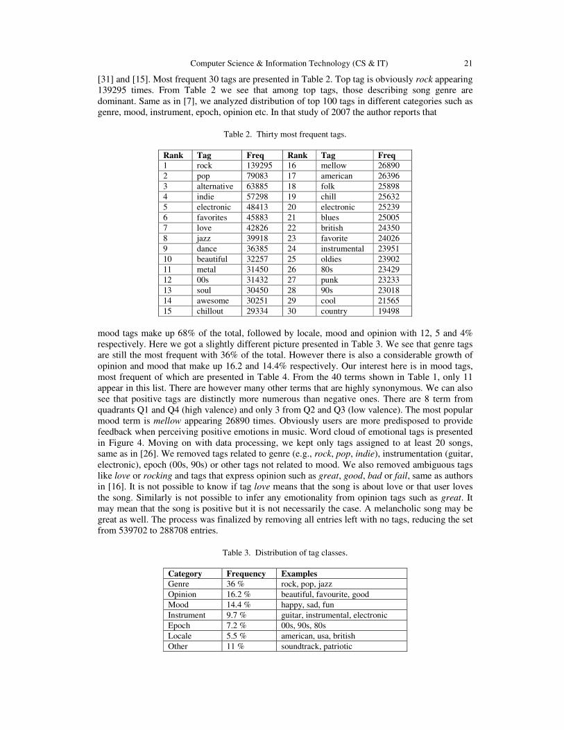
[31] and [15]. Most frequent 30 tags are presented in Table 2. Top tag is obviously rock appearing
139295 times. From Table 2 we see that among top tags, those describing song genre are
dominant. Same as in [7], we analyzed distribution of top 100 tags in different categories such as
genre, mood, instrument, epoch, opinion etc. In that study of 2007 the author reports that
Table 2. Thirty most frequent tags.
Rank Tag Freq Rank Tag Freq
1 rock 139295 16 mellow 26890
2 pop 79083 17 american 26396
3 alternative 63885 18 folk 25898
4 indie 57298 19 chill 25632
5 electronic 48413 20 electronic 25239
6 favorites 45883 21 blues 25005
7 love 42826 22 british 24350
8 jazz 39918 23 favorite 24026
9 dance 36385 24 instrumental 23951
10 beautiful 32257 25 oldies 23902
11 metal 31450 26 80s 23429
12 00s 31432 27 punk 23233
13 soul 30450 28 90s 23018
14 awesome 30251 29 cool 21565
15 chillout 29334 30 country 19498
mood tags make up 68% of the total, followed by locale, mood and opinion with 12, 5 and 4%
respectively. Here we got a slightly different picture presented in Table 3. We see that genre tags
are still the most frequent with 36% of the total. However there is also a considerable growth of
opinion and mood that make up 16.2 and 14.4% respectively. Our interest here is in mood tags,
most frequent of which are presented in Table 4. From the 40 terms shown in Table 1, only 11
appear in this list. There are however many other terms that are highly synonymous. We can also
see that positive tags are distinctly more numerous than negative ones. There are 8 term from
quadrants Q1 and Q4 (high valence) and only 3 from Q2 and Q3 (low valence). The most popular
mood term is mellow appearing 26890 times. Obviously users are more predisposed to provide
feedback when perceiving positive emotions in music. Word cloud of emotional tags is presented
in Figure 4. Moving on with data processing, we kept only tags assigned to at least 20 songs,
same as in [26]. We removed tags related to genre (e.g., rock, pop, indie), instrumentation (guitar,
electronic), epoch (00s, 90s) or other tags not related to mood. We also removed ambiguous tags
like love or rocking and tags that express opinion such as great, good, bad or fail, same as authors
in [16]. It is not possible to know if tag love means that the song is about love or that user loves
the song. Similarly is not possible to infer any emotionality from opinion tags such as great. It
may mean that the song is positive but it is not necessarily the case. A melancholic song may be
great as well. The process was finalized by removing all entries left with no tags, reducing the set
from 539702 to 288708 entries.
Table 3. Distribution of tag classes.
Category Frequency Examples
Genre 36 % rock, pop, jazz
Opinion 16.2 % beautiful, favourite, good
Mood 14.4 % happy, sad, fun
Instrument 9.7 % guitar, instrumental, electronic
Epoch 7.2 % 00s, 90s, 80s
Locale 5.5 % american, usa, british
Other 11 % soundtrack, patriotic

22 Computer Science & Information Technology (CS & IT)
Table 4. Thirty most frequent mood tags.
Rank Tag Freq Rank Tag Freq
16 mellow 26890 103 soft 7164
40 funk 16324 107 energetic 6827
45 fun 14777 109 groovy 6771
50 happy 13633 127 uplifting 5188
52 sad 13391 138 calm 4769
59 melancholy 12025 145 emotional 4515
63 smooth 11494 153 funny 4034
66 relax 10838 157 cute 3993
68 upbeat 10641 227 quirky 2606
69 relaxing 10513 230 moody 2549
78 melancholic 9392 231 quiet 2538
90 atmospheric 8149 236 bittersweet 2458
93 sweet 8006 241 angry 2361
96 dark 7668 242 soothing 2361
99 dreamy 7296 291 sentimental 1937
5. ANNOTATION SCHEME AND RESULTS
At this point what’s left is the identification of the tracks that can be distinctly fitted in one of the
4 mood clusters we defined, based on the tags they have received. To make use of as much
Figure 4. Cloud of most frequent affect tags
tags as possible and reach to a large dataset (third requirement), we extend the basic 10 terms of
each cluster with their related forms derived from lemmatization process. For example, is makes
sense to assume that relaxing, relax and relaxation tags express the same opinion as relaxed
which is part of cluster 4. We reached to a final set of 147 words that were the most meaningful
from music emotion perspective. The next step was to identify and count those tags in each song.
At the end of this step, for each song we had 4 counters, representing the number of tags from
each mood cluster. To keep in highly polarized songs only and thus fulfill the first requirement,
we implemented a tight scheme denoted as 4-0 or 6-1 or 9-2 or 14-3. It means that a song is set to
quadrant Qx if either one of the following conditions is fulfilled:
• It has 4 or more tags of Qx and no tags of any other quadrant
• It has 6 up to 8 tags of Qx and at most 1 tag of any other quadrant

Computer Science & Information Technology (CS & IT) 23
• It has 9 up to 13 tags of Qx and at most 2 tags of any other quadrant
• It has 14 or more tags of Qx and at most 3 tags of any other quadrant
Songs with 3 or fewer tags or not fulfilling one of the above conditions were discarded. The
remaining set was a collection of 1986 happy, 574 angry, 783 sad and 1732 relaxed songs for a
total of 5075. From this numbers we can see that the dataset we obtained is clearly imbalanced,
with more songs being reported as positive (3718 in Q1 and Q4) and fewer as negative (only 1357
in Q2 and Q3). This is something we expected, since as we reported in the previous section, tag
distribution was imbalanced in the same way.
The pos-neg representation is clearly oversimplified and does not reveal much about song
emotionality. Nevertheless, such datasets are usually highly polarized. Positive and negative
terms are easier to distinguish. Same happens with several types of features that are often used for
classification. The confidence of a binary categorization is usually higher not just in music but in
other application domains as well. The pos-neg lyrics dataset we created here might be very
useful for training and exercising many sentiment analysis or machine learning algorithms. We
added more terms in the two categories, terms that couldn’t be used with the 4 class annotation
scheme. For example, tags like passionate, confident and elegant are positive, even though they
are not distinctly happy or relaxed. Same happens with wry, paranoid and spooky on the negative
side. We used valence norm of ANEW as an indicator of term positivity and reached to a final set
of 557 terms. Given the fact that positive and negative terms were more numerous, for pos-neg
classification we implemented 5-0 or 8-1 or 12-2 or 16-3 scheme which is even tighter. A song is
considered to have positive or negative mood if it has 5 or more, 8-11, 12-15, or more than 15
tags of that category and 0, at most 1, 2, or at most 3 tags of the other category. Using this scheme
we got a set of 2589 negative and 5940 positive songs for a total of 8529. Same as above, we see
that positive songs are more numerous.
6. CONCLUSIONS
In this paper we presented the steps that we followed for the creation of two datasets of mood
annotated lyrics based on last.fm user tags of each song. We started from two large and popular
music data collections, Playlist and MSD. As music emotion model, we adopted a mood space of
4 term clusters, very similar to the popular model of Russell which has been proved effective in
many studies. Analyzing last.fm tags of songs, we observed that despite the growth of opinion
and mood tags, genre tags are still the most numerous. Within mood tags, those expressing
positive emotions (happy and relaxed) are dominant. For the classification of songs we used a
stringent scheme that annotates each track based on its tag counters, guaranteeing polarized
clusters of songs. The two resulting datasets are imbalanced, containing higher number of positive
songs and reflecting the bias of user tags that were provided. Both datasets will be available for
public use. Any feedback regarding the annotation quality of the data is appreciated. Researchers
are also invited to extend the datasets, especially the smaller clusters of songs.
ACKNOWLEDGEMENTS
This work was supported by a fellowship from TIM
9. Computational resources were provided by
HPC@POLITO10
, a project of Academic Computing within the Department of Control and
Computer Engineering at Politecnico di Torino.
9 https://www.tim.it/
10 http://hpc.polito.it

24 Computer Science & Information Technology (CS & IT)
REFERENCES
[1] D. Tang, B. Qin, and T. Liu. Deep learning for sentiment analysis: Successful approaches and future
challenges. Wiley Int. Rev. Data Min. and Knowl. Disc., 5(6):292–303, Nov. 2015.
[2] Giz H. He, J. Jin, Y. Xiong, B. Chen, W. Sun, and L. Zhao. Language Feature Mining for Music
Emotion Classification via Supervised Learning from Lyrics, pages 426–435. Springer Berlin
Heidelberg, Berlin, Heidelberg, 2008.
[3] M. van Zaanen and P. Kanters. Automatic mood classification using tf*idf based on lyrics. In J. S.
Downie and R. C. Veltkamp, editors, ISMIR, pages 75–80. International Society for Music
Information Retrieval, 2010.
[4] H.-C. Kwon and M. Kim. Lyrics-based emotion classification using feature selection by partial
syntactic analysis. 2011 IEEE 23rd International Conference on Tools with Artificial Intelligence
(ICTAI 2011), 00:960–964, 2011.
[5] J. H. Lee and X. Hu. Generating ground truth for music mood classification using mechanical turk. In
Proceedings of the 12th ACM/IEEE-CS Joint Conference on Digital Libraries, JCDL ’12, pages 129–
138, New York, NY, USA, 2012. ACM.
[6] J. A. Speck, E. M. Schmidt, B. G. Morton, and Y. E. Kim. A comparative study of collaborative vs.
traditional musical mood annotation. In A. Klapuri and C. Leider, editors, ISMIR, pages 549–554.
University of Miami, 2011.
[7] P. Lamere and E. Pampalk. Social tags and music information retrieval. In ISMIR 2008, 9th
International Conference on Music Information Retrieval, Drexel University, Philadelphia, PA, USA,
September 14-18, 2008, page 24, 2008.
[8] X. Hu and J. S. Downie. When lyrics outperform audio for music mood classification: A feature
analysis. In J. S. Downie and R. C. Veltkamp, editors, ISMIR, pages 619–624. International Society
for Music Information Retrieval, 2010.
[9] C. Laurier, M. Sordo, J. Serr, and P. Herrera. Music mood representations from social tags. In K.
Hirata, G. Tzanetakis, and K. Yoshii, editors, ISMIR, pages 381–386. International Society for Music
Information Retrieval, 2009.
[10] K. Bischoff, C. S. Firan, R. Paiu, W. Nejdl, C. Laurier, and M. Sordo. Music mood and theme
classification - a hybrid approach. In Proceedings of the 10th International Society for Music
Information Retrieval Conference, ISMIR 2009, Kobe International Conference Center, Kobe, Japan,
October 26-30, 2009, pages 657–662, 2009.
[11] X. Hu, M. Bay, and J. Downie. Creating a simplified music mood classification groundtruth set. In
Proceedings of the 8th International Conference on Music Information Retrieval (ISMIR 2007), 2007.
[12] A. L. Maas, R. E. Daly, P. T. Pham, D. Huang, A. Y. Ng, and C. Potts. Learning word vectors for
sentiment analysis. In Proceedings of the 49th Annual Meeting of the Association for Computational
Linguistics: Human Language Technologies - Volume 1, HLT ’11, pages 142–150, Stroudsburg, PA,
USA, 2011. Association for Computational Linguistics.
[13] Y. E. Kim, E. M. Schmidt, R. Migneco, B. G. Morton, P. Richardson, J. Scott, J. A. Speck, and D.
Turnbull. State of the art report: Music emotion recognition: A state of the art review. In Proceedings
of the 11th International Society for Music Information Retrieval Conference, pages 255–266,
Utrecht, The Netherlands, August 9-13 2010. http://ismir2010.ismir.net/proceedings/ismir2010-
45.pdf.
[14] Z. Fu, G. Lu, K. M. Ting, and D. Zhang. A survey of audio-based music classification and annotation.
IEEE Transactions on Multimedia, 13(2):303–319, April 2011.
Computer Science & Information Technology (CS & IT) 25
[15] X. Hu and J. S. Downie. Exploring mood metadata: Relationships with genre, artist and usage
metadata. In Proceedings of the 8th International Conference on Music Information Retrieval, pages
67–72, Vienna, Austria, September 23-27 2007.
http://ismir2007. ismir.net/proceedings/ISMIR2007_p067_hu.pdf.
[16] X. Hu, J. S. Downie, and A. F. Ehmann. Lyric text mining in music mood classification. In K. Hirata,
G. Tzanetakis, and K. Yoshii, editors, ISMIR, pages 411–416. International Society for Music
Information Retrieval, 2009.
[17] X. Hu and J. S. Downie. Improving mood classification in music digital libraries by combining lyrics
and audio. In Proceedings of the 10th Annual Joint Conference on Digital Libraries, JCDL ’10, pages
159–168, New York, NY, USA, 2010. ACM.
[18] R. Malheiro, R. Panda, P. Gomes, and R. P. Paiva. Classification and regression of music lyrics:
Emotionally-significant features. In A. L. N. Fred, J. L. G. Dietz, D. Aveiro, K. Liu, J. Bernardino,
and J. Filipe, editors, KDIR, pages 45–55. SciTePress, 2016.
[19] J. A. Russell. A circumplex model of affect. Journal of Personality and Social Psychology, 39:1161–
1178, 1980.
[20] M. M. Bradley and P. J. Lang. Affective norms for English words (ANEW): Stimuli, instruction
manual, and affective ratings. Technical report, Center for Research in Psychophysiology, University
of Florida, Gainesville, Florida, 1999.
[21] D. Turnbull, L. Barrington, D. A. Torres, and G. R. G. Lanckriet. Semantic annotation and retrieval of
music and sound effects. IEEE Trans. Audio, Speech & Language Processing, 16(2):467–476, 2008.
[22] E. Çano and M. Morisio, Moodylyrics: A sentiment annotated lyrics dataset, in Proceedings of the
2017 International Conference on Intelligent Systems, Metaheuristics & Swarm Intelligence, ISMSI
’17, ACM, Hong Kong, March 2017, pp. 118–124. doi:10.1145/3059336.3059340.
[23] K. Trohidis, G. Tsoumakas, G. Kalliris, and I. Vlahavas. Multi-label classification of music into
emotions. In Proceedings of the 9th International Conference on Music Information Retrieval, pages
325–330, Philadelphia, USA, September 14-18 2008.
http://ismir2008.ismir.net/papers/ISMIR2008_275.pdf.
[24] A. Tellegen, D. Watson, and L. A. Clark. On the dimensional and hierarchical structure of affect.
Psychological Science, 10(4):297–303, 1999.
[25] R. Mihalcea and C. Strapparava. Lyrics, music, and emotions. In Proceedings of the 2012 Joint
Conference on Empirical Methods in Natural Language Processing and Computational Natural
Language Learning, EMNLP-CoNLL 2012, July 12-14, 2012, Jeju Island, Korea, pages 590–599,
2012.
[26] M. Schedl, C. C. Liem, G. Peeters, and N. Orio. A Professionally Annotated and Enriched
Multimodal Data Set on Popular Music. In Proceedings of the 4th ACM Multimedia Systems
Conference (MMSys 2013), Oslo, Norway, February–March 2013.
[27] K. Hevner. Experimental studies of the elements of expression in music. The American Journal of
Psychology, 48(2):246–268, 1936.
[28] D. Tang, B. Qin, and T. Liu. Deep learning for sentiment analysis: Successful approaches and future
challenges. Wiley Int. Rev. Data Min. and Knowl. Disc., 5(6):292–303, Nov. 2015.
[29] T. Mikolov, I. Sutskever, K. Chen, G. S. Corrado, and J. Dean. Distributed representations of words
and phrases and their compositionality. In C. J. C. Burges, L. Bottou, M. Welling, Z. Ghahramani,
and K. Q. Weinberger, editors, Advances in Neural Information Processing Systems 26, pages 3111–
3119. Curran Associates, Inc., 2013.

26 Computer Science & Information Technology (CS & IT)
[30] T. Bertin-Mahieux, D. P. Ellis, B. Whitman, and P. Lamere. The million song dataset. In Proceedings
of the 12th International Conference on Music Information Retrieval (ISMIR 2011), 2011.
[31] Y.-C. Lin, Y.-H. Yang, and H. H. Chen. Exploiting online music tags for music emotion
classification. TOMCCAP, 7(Supplement):26, 2011.
[32] S. Chen, J. L. Moore, D. Turnbull, and T. Joachims. Playlist prediction via metric embedding. In
Proceedings of the 18th ACM SIGKDD International Conference on Knowledge Discovery and Data
Mining, KDD ’12, pages 714–722, New York, NY, USA, 2012. ACM.

David C. Wyld et al. (Eds) : CCSEIT, AIAP, DMDB, ICBB, CNSA - 2017
pp. 27– 34, 2017. © CS & IT-CSCP 2017 DOI : 10.5121/csit.2017.70604
EFFECTIVE VECTOR REPRESENTATIONS
FOR VARIABLE LENGTH SYMBOL
SEQUENCES
Gustavo Lado and Enrique Carlos Segura
Facultad de Ciencias Exactas y Naturales, Universidad de Buenos Aires
ABSTRACT
Machine learning techniques have demonstrated their versatility and have been successfully
applied to a wide variety of problems. However, one of their major limitations is the treatment
of sequential information. In general the input and output for these methods is expressed as
fixed-dimension vectors, but in many problem domains, as in natural language processing, the
information is represented by variable-length sequences. In most cases, it is possible to use
some methods that transform these variable length sequences into fixed dimension vectors, but
each of these methods has its own disadvantages. In this paper we propose an alternative to
obtain vector representations of fixed dimension from sequences of symbols of variable length
and their potential applications for natural language processing..
KEYWORDS
Neural Networks, Natural Language Processing, Sequential Learning, Deep Architectures
1. INTRODUCTION
One of the main topics of interest in the area of machine learning is natural language processing,
but despite the excellent results that have been obtained there is still a barrier that is difficult to
overcome [1]. Most machine learning techniques are designed to work with instantaneous
information represented in the form of vectors; natural language, however, is always presented as
sequential information. Whether we consider words as sequences of letters, sentences as
sequences of words, or documents as sequences of sentences, in all these cases we may think that
information is presented as a sequence of symbols, and in order to effectively use these machine
learning techniques we need, in some way, to transform this sequential information into a vector
representation. But what kind of such representation we want to obtain? [2]
For example, it is desirable that the vector representation be directly related to the symbols
forming the sequence, not only indicating which symbols are present, or their quantity, but also in
their order [3]. Ideally the vector representation will have enough information about the sequence
so as to make it possible its reconstruction.
It is also desirable that the vector representation obtained have the smallest possible dimension
[4]. Some degree of redundancy may be acceptable for error correction, but given the nature and
possible applications of this method every extra dimension in the representation can carry a
computational load in later stages.

28 Computer Science & Information Technology (CS & IT)
An important point for the vector representation is to be consistent across all valid sequences. For
example, similar sequences should have similar vector representations, so that the vector distance
between two different representations could be used to measure the similarity of the sequences to
which they correspond.
Ideally the representations could be so consistent as to end up supporting vector operations with
constraints but responding to a certain degree of compositionality [5]. For example, it might be
useful if arithmetic operations could be performed on the vector representations to obtain a
representation close to the result of doing the same operations on the original sequences.
And finally it is desirable that the method be effective, i.e., that it be possible to encode any valid
sequence easily. This means that it is possible to accept restrictions on what is considered a valid
sequence, for example, in the set of possible symbols or in the maximum length, but once these
restrictions are accepted the codification should be possible without consuming many
computational resources. Furthermore the method has to be efficient [6]. This means that the
training should be performed relatively quickly even for large datasets, and ideally must have an
acceptable degree of generalization for any valid sequence.
2. BACKGROUND AND MOTIVATION
Currently, there are several methods that offer similar solutions. We will consider next some of
the most commonly used to evaluate how they behave in relation to all the properties described
above.
One of the most used is known as Bag of Words [7]. With this method, each sentence or
document is represented by a vector with as many dimensions as words contain a dictionary. Each
position in this vector corresponds to the number of times that a specific word of the dictionary
appears in the sequence. This type of vectors have the advantage of being easily generated with
great consistency between sequences. But they present the problem of discarding a large amount
of information and the result is usually of such a large dimension that it is rarely used directly
without going through a later stage of dimensionality reduction.
Another of the first models to consider vector representations for sequence processing were the
Simple Recurrent Neural Networks [8]. In this case, the previous state of the hidden layer of a
neural network is used as part of the input during training to try to predict the next item in the
sequence. This method can effectively generate vector representations in the hidden layer, even
with a low dimension, and the result is completely consistent for any valid sequence. However,
the same recurring nature of the architecture generates problems with the back-propagation
training, making the method only able to be effectively used for small datasets.
An alternative to try to deal with this problem are the so-called Long-Short Term Memory
networks [9]. They use a type of unit with several internal connections to be able to decide which
information is propagated at any time. This allows them to use multiple hidden layers to work
with much larger data sets. But the same use of this type of units not only makes the training
more complex, but also makes it impossible to obtain a single vector representation with all the
corresponding information for each sequence.
There is also another not-so-known model called Recursive Auto-Associative Memory (RAAM)
[10] which is, in a way, a generalization of Elman's simple recurrent network model [8]. A
RAAM network is composed of an auto-encoder capable of compressing a pair of patterns to only
one of smaller dimension. This new compressed patterns can be recursively fed back into the
network, allowing it to learn to encode and decode complex data structures such as lists and trees.
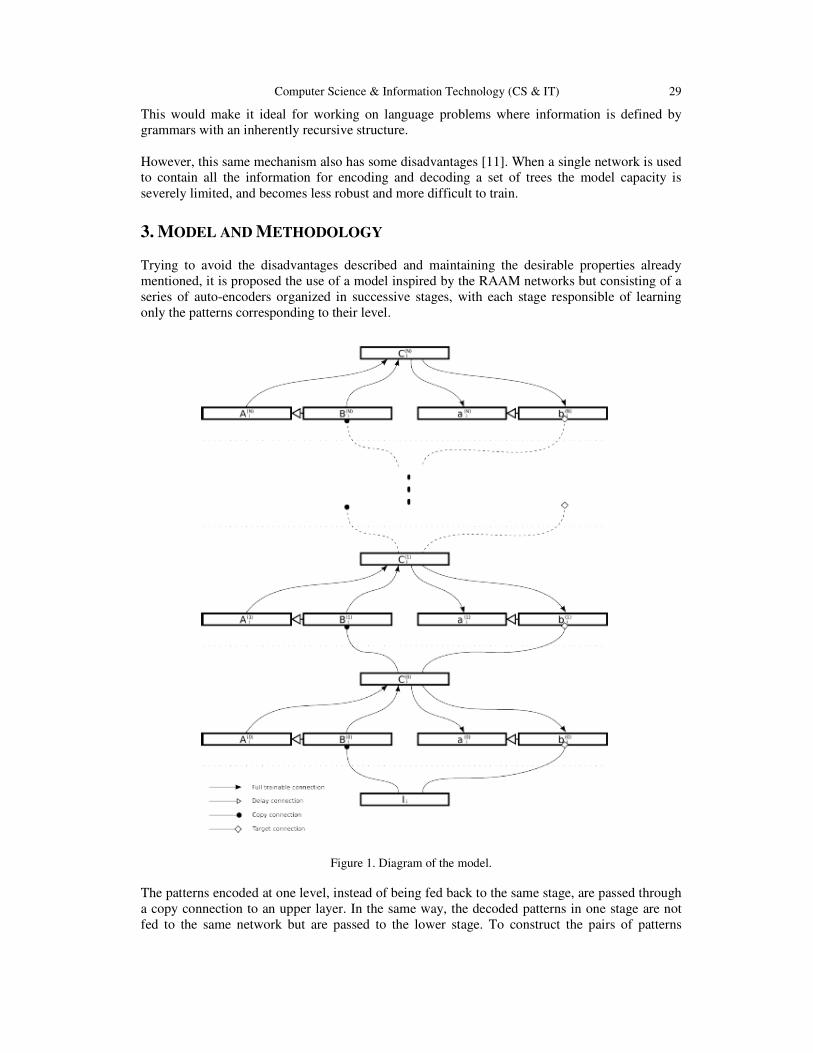
Computer Science & Information Technology (CS & IT) 29
This would make it ideal for working on language problems where information is defined by
grammars with an inherently recursive structure.
However, this same mechanism also has some disadvantages [11]. When a single network is used
to contain all the information for encoding and decoding a set of trees the model capacity is
severely limited, and becomes less robust and more difficult to train.
3. MODEL AND METHODOLOGY
Trying to avoid the disadvantages described and maintaining the desirable properties already
mentioned, it is proposed the use of a model inspired by the RAAM networks but consisting of a
series of auto-encoders organized in successive stages, with each stage responsible of learning
only the patterns corresponding to their level.
Figure 1. Diagram of the model.
The patterns encoded at one level, instead of being fed back to the same stage, are passed through
a copy connection to an upper layer. In the same way, the decoded patterns in one stage are not
fed to the same network but are passed to the lower stage. To construct the pairs of patterns

30 Computer Science & Information Technology (CS & IT)
corresponding to each stage a type of delayed connection is used which is responsible for the
coordination.
In this way, each stage should only learn the regularities corresponding to its level, that is, the
first level learns about regularities between pairs of letters, the next about regularities between
pairs of pairs of letters and so on [12]. This increases the capacity of the model since the network
at each stage should only learn a part of the set of patterns that previously had to learn a single
network, making it also less prone to failures.
Figure 1 shows a diagram of the model. The stages are separated by dotted lines. Each stage has
an auto-encoder similar to the one on a RAAM network, where the input is formed by layers A
and B, the hidden part by layer C, and the output by the layers a and b. In all these layers the
position within the sequence is indicated by the subscript i and the corresponding stage with a
superscript (n).
The input sequence will be defined by I = [ I0, I1, … IL ] wherein each Ii is a vector representing a
symbol. At the bottom, layer Ii indicates the pattern at position i in the input sequence.
At each stage j the encoding and decoding corresponding to the position i within the sequence are
described by:
[ Ai(j), Bi
(j) ] → [ Ci(j) ] → [ ai
(j), bi(j) ]
In turn, each stage j will produce a sequence C(j) = [ C0(j), C1
(j), … CM(j) ] in which each Ci
(j) is also
a vector [13]. One of the objectives of this architecture is that each stage encodes a sequence of
less or equal length, that is to say, to produce sequences that comply with |C(j)
| >= |C(j+1)
| until
finally |C(N)|=1, where N is the number of stages.
Trainable, copy, delayed and target connections are indicated with different types of lines in the
same figure. The copy and delay connections work together to define the pairs of patterns that
each stage must learn. For the first stage the input patterns to the network are defined by:
[ Ai(0), Bi
(0) ] = [ Ii, Ii+1 ]
For the successive stages it is possible to choose between two ways of selecting the pattern pairs
depending on the level of redundancy that is desired. For example it is possible to switch between
two different methods defined by:
[ Ai(j)
, Bi(j)
] = [ C2i(j-1)
, C2i+1(j-1)
] if j is even
[ Ai(j)
, Bi(j)
] = [ Ci(j-1)
, Ci+1(j-1)
] if j is odd
Note that this makes |C(j)| = 2|C(j+1)| if j is even and |C(j)| = |C(j+1)|+1 if j is odd, fulfilling the
required |C(j)
| >= |C(j+1)
| condition. Also note that in cases where j is odd is met Ai+1(j)
= Bi(j)
, this
introduces the level of redundancy in the patterns at the time of decoding that makes the model
more robust [14]. In each case the targets for [ ai(j), bi
(j) ] are equal to the values of [ Ai(j), Bi
(j) ]
previously determined.
4. RESULTS
In order to demonstrate its properties a model consisting of 7 stages capable of coding letter
sequences was used, where the letters are represented by bipolar patterns of dimension 8. The
number of units used in each stage was chosen depending on the amount of combinations of pairs

Computer Science & Information Technology (CS & IT) 31
of patterns produced by the previous stage. Finally the vector produced by the final stage has a
size of 128 bipolar values. These vectors are represented in the figures with black and white
squares corresponding to the positive and negative values.
The model was trained with a set of 1000 random words from the English language. In order to
demonstrate some of the desired properties, it was necessary to ensure that 9 of the words were
related to “every” and “sing” as shown in the examples below. It is important to note that vector
representations do not have, neither are intended to have, any information about the meaning of
the words. It is a purely syntactic, non-semantic representation.
The first results consist of some pairs of words whose vectors have the smallest mutual distances
of the whole set. In this case the values of the distances between the pairs of vectors are not being
included because the vector representations are sufficiently similar between them (Figure 2).
Figure 2. Words from the dataset with the similar vector representations.
In particular, it is interesting to show how similar words obtain similar vector representations, and
how these representations can be used to identify words belonging to a group or family [5,13].
Also, comparing three words with different root but same syntactic category, it can be seen how it
would be possible to use this type of representation to identify to which category a new word
belongs.
Another interesting aspect to note is the ability to detect typographical errors [15]. As part of the
training set, the words "every", "ever" and "fever" were included as all valid and similar to each
other, and compared to three types of errors (replacement, omission and addition of one letter)
with respect to "every" (Figure 3).
Figure 3. Vector representations from words similar to “every”.
In this case we compare the distances between the representations of some valid words similar to
"every" and other vector representations obtained from variations with typographical errors.
dist(every,ever) = 13.227 dist(every,ebery) = 12.867
dist(ever,fever) = 13.239 dist(every,evry) = 12.982
dist(every,fever) = 13.631 dist(every,everyy) = 13.695
A potential application of the information obtained with this method is the possibility to identify
an unknown word either as a poorly written word or as a new word. If it is a known word but

32 Computer Science & Information Technology (CS & IT)
poorly written, its vector representation should be sufficiently similar to the original word (ie, low
vector distance between them).
Figure 4. Vector representations from words similar to “singing”.
In the next test (Figure 4) it is shown how it would be possible to infer information of an
unknown word from known words [16]. In this case the model was trained with some words as
"sing", "sings", "song" and some gerunds as "sinking", "ringing" and "swinging", and it was
analyzed what type of representation would be obtained for an unknown word, but associated to
these two groups, like "singing".
dist(sing,sings) = 14.344 dist(sinking,singing) = 12.912
dist(sing,song) = 14.152 dist(ringing,singing) = 13.536
dist(sings,song) = 15.059 dist(swinging,singing) = 15.301
In this case it can be seen that the distance between two similar but known words is usually
greater than the distance with a new word which is associated with known words. However, the
real measure is to see how adequate the representation of the new word is in relation to the known
groups of words [5,11].
dist( sinking-sink+sing, singing) = 10.781
dist( ringing-ring+sing, singing) = 10.269
dist( swinging-swing+sing, singing) = 11.723
These representations obtained by performing arithmetic operations on the vectors were not only
very similar to the representation of the new word, but also very similar to each other, showing
that the representations generated by this method are consistent for different sequences.
5. CONCLUSIONS AND FUTURE WORK
In this paper we explored the possibilities of the proposed method applied to sequences of letters,
that is to say, words; but it is clear that this same principle can be applied to sequences of words,
and even sequences of sentences. The case of word coding is simple enough to easily show the
properties of the model and can also be used as a first step in more complex coding. However
working exclusively with a natural language is not enough to show its true flexibility.
A good demonstration of the capability of the model would be to test it against randomly
generated sequences from regular and context-free grammars and measuring its properties against
different levels of entropy.
Another aspect to consider is the memory capacity of the model, specifically what is the
minimum number of units needed at each stage for it to be able to reconstruct all known

Computer Science & Information Technology (CS & IT) 33
sequences without errors, and the number of stages needed with the proper methods of pattern
pairing in order to have an adequate level of redundancy.
REFERENCES
[1] Dietterich, T.G., 2002, August. Machine learning for sequential data: A review. In Joint IAPR
International Workshops on Statistical Techniques in Pattern Recognition (SPR) and Structural and
Syntactic Pattern Recognition (SSPR) (pp. 15-30). Springer Berlin Heidelberg.
[2] David E. Rumelhart, Geoffrey E. Hinton, and Ronald J. Williams. 1988. Learning representations by
back-propagating errors. In Neurocomputing: foundations of research, James A. Anderson and
Edward Rosenfeld (Eds.). MIT Press, Cambridge, MA, USA 696-699.
[3] Socher, R., Lin, C.C., Manning, C. and Ng, A.Y., 2011. Parsing natural scenes and natural language
with recursive neural networks. In Proceedings of the 28th international conference on machine
learning (ICML-11) (pp. 129-136).
[4] Sutskever, I. and Hinton, G.E., 2007, March. Learning Multilevel Distributed Representations for
High-Dimensional Sequences. In AISTATS (Vol. 2, pp. 548-555).
[5] Mikolov, T., Sutskever, I., Chen, K., Corrado, G.S. and Dean, J., 2013. Distributed representations of
words and phrases and their compositionality. In Advances in neural information processing systems
(pp. 3111-3119).
[6] LeCun, Y.A., Bottou, L., Orr, G.B. and Müller, K.R., 2012. Efficient backprop. In Neural networks:
Tricks of the trade (pp. 9-48). Springer Berlin Heidelberg.
[7] Wallach, H.M., 2006, June. Topic modeling: beyond bag-of-words. In Proceedings of the 23rd
international conference on Machine learning (pp. 977-984). ACM.
[8] Elman, J. L. 1990. Finding structure in time. Cognitive science, 14(2), 179-211.
[9] Sepp Hochreiter and Jürgen Schmidhuber. 1997. Long Short-Term Memory. Neural Comput. 9, 8
(November 1997), 1735-1780.
[10] Pollack, J.B., 1990. Recursive distributed representations. Artificial Intelligence, 46(1), pp.77-105.
[11] Levy, S., Melnik, O. and Pollack, J., 2000, February. Infinite RAAM: a principled connectionist basis
for grammatical competence. In Proceedings of the 22nd annual meeting of the cognitive science
society (pp. 298-303).
[12] Hinton, G.E., 2007. Learning multiple layers of representation. Trends in cognitive sciences, 11(10),
pp.428-434.
[13] Hinton, G.E. and Salakhutdinov, R.R., 2006. Reducing the dimensionality of data with neural
networks. science, 313(5786), pp.504-507.
[14] Vincent, P., Larochelle, H., Lajoie, I., Bengio, Y. and Manzagol, P.A., 2010. Stacked denoising
autoencoders: Learning useful representations in a deep network with a local denoising criterion.
Journal of Machine Learning Research, 11(Dec), pp.3371-3408.
[15] Li, Y., Cohn, T. and Baldwin, T., 2016. Learning robust representations of text. arXiv preprint
arXiv:1609.06082.
[16] Ravuri, S. and Stolcke, A., 2016, March. A comparative study of recurrent neural network models for
lexical domain classification. In Acoustics, Speech and Signal Processing (ICASSP), 2016 IEEE
International Conference on (pp. 6075-6079). IEEE.
34 Computer Science & Information Technology (CS & IT)
AUTHORS
Gustavo Lado is a graduated student from the University of Buenos Aires in
Computing Science.
His previous research interests include the simulation of the human visual system
with artificial neural networks. Part of this work was recently published in the book
"La Percepción del Hombre y sus Máquinas".
He is currently working in neural networks applied to the natural language processing and cognitive
semantics as part his Ph.D.
Enrique Carlos Segura was born in Buenos Aires, Argentina. He received the M.Sc.
degrees in Mathematics and Computer Science in 1988 and the Ph.D. degree in
Mathematics in 1999, all from University of Buenos Aires.
He was Fellow at the CONICET (National Research Council, Argentina) and at the
CONEA (Atomic Energy Agency, Argentina). He had also a Thalmann Fellowship to
work at the Universitat Politécnica de Catalunya (Spain) and a Research Fellowship at South Bank
University (London). From 2003 to 2005 he was Director of the Department of Computer Science of the
University of Buenos Aires, where he is at present a Professor and Resarcher.
His main areas of research are Artificial neural Networks -theory and applications- and, in general,
Cognitive Models of Learning and Memory.

David C. Wyld et al. (Eds) : CCSEIT, AIAP, DMDB, ICBB, CNSA - 2017
pp. 35– 52, 2017. © CS & IT-CSCP 2017 DOI : 10.5121/csit.2017.70605
CLUSTERING FOR DIFFERENT SCALES OF
MEASUREMENT - THE GAP RATIO
WEIGHTED K-MEANS ALGORITHM
Joris Guerin, Olivier Gibaru, Stephane Thiery and Eric Nyiri
Laboratoire des Sciences de l'Information et des Systemes (CNRS UMR 7296)
Arts et Metiers ParisTech, Lille, France
ABSTRACT
This paper describes a method for clustering data that are spread out over large regions and
which dimensions are on different scales of measurement. Such an algorithm was developed to
implement a robotics application consisting in sorting and storing objects in an unsupervised
way. The toy dataset used to validate such application consists of Lego bricks of different
shapes and colors. The uncontrolled lighting conditions together with the use of RGB color
features, respectively involve data with a large spread and different levels of measurement
between data dimensions. To overcome the combination of these two characteristics in the data,
we use a weighted K-means algorithm which consists in weighting each dimension of the feature
space before running K-means. The novelty of this paper lies in the introduction of new weights,
relevant for the combination of large spread and different scales. The weight associated with a
feature is proportional to the ratio of the biggest gap between two consecutive data points, and
the average of all the other gaps. We call this algorithm gap-ratio K-means. This method is
compared with two other variants of K-means on the Lego bricks clustering problem as well as
two other common classification datasets.
KEYWORDS
Unsupervised Learning, Weighted K-means, Scales of measurement, Robotics application
1. INTRODUCTION
1.1 MOTIVATIONS
In a relatively close future, we are likely to see industrial robots performing tasks on their own. In
this perspective, we have developed a smart table cleaning application in which a robot sorts and
store objects judiciously among the storage areas available. This clustering application can have
different uses: workspaces can be organized before the workday, unsorted goods can be sorted
before packaging, .... Even in domestic robotics, such an application, dealing with real objects,
can be useful to perform household chores.
As shown in Figure 1, a Kuka LBR iiwa collaborative robot equipped with a camera is presented
a table cluttered with unsorted objects. Color and shape features of each object are extracted and

36 Computer Science & Information Technology (CS & IT)
the algorithm clusters the data in as many classes as there are storage bins. Once objects have
been labelled with bin numbers, the robot physically cleans up the table. A better description of
the experiment is given in the body of the article. This application was tested with Lego bricks of
different colors and shapes (see section 4.2). A link to a demonstration video is given in the
caption of Figure 1.
Because such application is meant for ordinary environments, the clustering algorithm needs to be
robust to unmastered light conditions, which is synonymous with widely spread datasets.
Moreover, the features chosen are on different levels of measurement [1]: RGB-color features are
interval type variables whereas lengths are on a ratio scale. Both these specificities of the
clustering problem motivated the development of a new weighted K-means algorithm, which is
the purpose of this paper.
Figure 1: KUKA LBR iiwa performing the Lego bricks sorting application.
Video at : https://www.youtube.com/watch?v=korkcYs1EHM
1.2 INTRODUCTION TO THE CLUSTERING PROBLEM
The table cleaning problem described above boils down to a clustering problem [2, 3]. Clustering
is a subfield of Machine Learning also called unsupervised classification. Given an unlabelled
dataset, the goal of clustering is to define groups among the entities. Members in one cluster
should be as similar as possible to each other and as different as possible to other clusters
members. In this paper, we are only concerned with parametric clustering, where the number of
clusters is a fixed parameter passed to the algorithm. However, we note that recently, non-
parametric Bayesian methods for clustering have been widely studied [4{6].
There are many possible definitions of similarity between data points. The choice of such
definition, together with the choice of the metric to optimize, differentiates between the different
clustering algorithms. The two surveys [7] and [8], give two slightly different classifications of
the various clustering algorithms.
After trying several clustering algorithms on simulated Lego bricks datasets using scikit-learn [9],
K-means clustering [10], a partitioning method, appeared efficient for our problem. Therefore,
among all clustering methods, this paper focuses on K-means.

Computer Science & Information Technology (CS & IT) 37
1.3. MAIN CONTRIBUTION
For certain unsupervised classification problems on data with large spread, a conventional
implementation of K-means algorithm can be inappropriate. Indeed, under certain lighting
conditions (not uniform throughout the scene), we observe absurd Lego bricks sorting. In order to
increase the clustering robustness, we try to emphasize the influence of certain features using
weighted K-means [11]. Weights based on coefficient of variation [12] (cv K-means) are tried
first. However, coefficient of variation only makes sense for data measured on a ratio scale,
which is not the case for our problem.
In this paper, we propose a new way to define weights in the framework of weighted K-means,
which works for both interval and ratio scaled data, we call gap-ratio K-means (gr K-means) the
resulting algorithm. In Section 4.2, we show that gr K-means is more robust than conventional K-
means and cv K-means for the Lego bricks sorting problem. The approach of exponentiating the
weights is also suggested. Introduction of gr K-means algorithm, together with an experimental
comparison with K-means and cv K-means on different datasets are the main contributions of this
paper.
The article is organized as follows, in Section 2, we briefly describe and derive both the K-means
and the cv K-means clustering methods as a baseline to understand the gr K-means algorithm,
explained in Sections 3. Between algorithms descriptions, intuitive explanations about why they
do not fit our problem are provided, data normalization before clustering is also discussed. In
Section 4, we propose an experimental validation of the efficiency of the gr K-means algorithm,
first on datasets constituted of Lego bricks, then on two other famous classification datasets.
Finally, we conclude this paper by suggesting our recommendations on how to handle a
clustering problem using K-means and give pointers to future work directions.
2. PRELIMINARIES
2.1 K-MEANS CLUSTERING
2.1.1 NOTATIONS
All along this paper, we try to respect the following notations. The use of letters i represents
indexing on data objects whereas letter j designates the features. Thus,
• X = { x1, ...., xi,..., xM } represents the dataset to cluster, composed of M data points.
• F = { f1,...., fj,... , fN } is the set of N features which characterize each data object.
• xij stands for the jth feature of object xi
A data object is represented by a vector in the feature space.
Likewise, the use of letter k represents the different clusters and
• C = { C1,...,Ck,....,CK } is a set of K clusters.

38 Computer Science & Information Technology (CS & IT)
K-means clustering is based on the concept of centroids. Each cluster Ck, is represented by a
cluster center, or centroid, denoted ck, which is simply a point in the feature space.
We also introduce d, the function used to measure dissimilarity between a data object and a
centroid. For K-means, such dissimilarity is quantified with Euclidean distance:
2.1.2 DERIVATION
Given a set of cluster centers c = { c1,…,ck,….,cK }, cluster membership is defined by
The goal of K-means is to find the set of cluster centers c* which minimizes the sum of
dissimilarities between each data object and its closest cluster center.
In practice, (3) is optimized by solving iteratively two subproblems, one where the set c is fixed
and one where A is fixed. The most widely used algorithm to implement K-means clustering is
the Lloyd's algorithm [13]. It is based on the method of Alternating Optimization [14], also used
in the Expectation-Maximization algorithm [15]. The K-means optimization is composed of two
main steps:
• The Expectation step (or E-step) :
� Initial situation : centroids are fixed (i.e., c is fixed)
� Action : Each data point in X is associated with a cluster following (2) (i.e., A is
computed).
• The Maximization step (or M-step) :
� Initial situation : Each data object is associated with a given cluster (i.e., A is
fixed).
� Action : For each cluster, the centroid that minimizes the total dissimilarity
within the cluster is computed (i.e., c is computed).

Computer Science & Information Technology (CS & IT) 39
When the norm used for dissimilarity is the L2 norm, which is the case for K-means, it can be
shown [10] that the M-step optimization is equivalent to computing the cluster mean:
2.1.3 CENTROID INITIALIZATION
In order to start iterating between the expectation and maximization steps, initial centroids need
to be defined. The choice of such initial cluster centers is crucial and motivates many research, as
shown in the survey paper [16]. The idea is to choose the initial centroids among the data points.
In our implementation, we use K-means++ algorithm [17] for clusters initialization (see Section
4.1).
2.1.4 DATA NORMALIZATION
In most cases, running K-means algorithm on raw data does not work well. Indeed, features with
largest scales are given more importance during dissimilarity calculation and clustering results are
biased. To deal with this issue, a common practice is to normalize the data before running the
clustering algorithm:
where µ j and σj represent respectively the empirical mean and variance of feature fj.
The made-up, two dimensional toy dataset in Figure 2 illustrates the interest of using data
normalization as a preprocessing to K-means. The two natural clusters in Figure 2 present similar
mean and variance, but expressed in different units, which makes K-means results completely
wrong without normalization.
However, reducing each feature distribution to a Gaussian of variance 1 can involve a loss of
valuable information for clustering. Weighted K-means [11] methods can solve such issue. The
underlying idea is to capture with weights relevant information about important features. This
information is reinjected in the data by multiplying each dimension with the corresponding
weight after normalization. In this way, the most relevant features for clustering are enlarged and
the others curtailed. In Sections 2.2.4 and 3, we propose two different weighted K-means
methods: cv K-means [12] and a new method that we call gap-ratio K-means (gr K-means). These
methods differ by the definition of the weights. We compare regular K-means, cv K-means and gr
K-means experimentally in Section 4.

40 Computer Science & Information Technology (CS & IT)
Figure 2: Toy data set to illustrate the need for data normalization before K-means.
2.2 WEIGHTED K-MEANS
2.2.1 ISSUES WITH DATA NORMALIZATION
As explained above, data normalization is often necessary to obtain satisfactory clustering results,
but involves a loss of information that can affect the quality of the clusters found. Weighted K-
means is based on the idea that information about the data can be captured before normalization
and reinjected in the normalized dataset.
2.2.2 WEIGHTED K-MEANS
In a weighted K-means algorithm, weights are attributed to each feature, giving them different
importance. Let us call wj the weight associated with feature fj. Then, the norm used in the E-step
of Weighted K-means is:
The difference between weighted K-means algorithms lies in the choice of the weights.
2.2.3 EXPONENTIAL WEIGHTED K-MEANS
In this paper, we also propose an extension of weighted K-means that consists in raising the
weights to the power of an integer p in the norm formula:

Computer Science & Information Technology (CS & IT) 41
By doing so, we emphasize even more the importance of features with large weights, which
makes sense if the information captured by the weights is relevant. In practice, as the weights are
between 0 and 1, p should not be too large to avoid considering only one feature. Influence of p in
the clustering results is studied in Section 4.
2.2.4 A PARTICULAR EXAMPLE : THE CV K-MEANS ALGORITHM
Weighted K-means based on coefficient of variation (cv K-means) [12] relies on the idea that the
variance of a feature is an good indicator of its importance for clustering. Such approach makes
sense, indeed, if two objects are of different nature because of a certain feature, the values of this
feature come from different distributions, which increases the internal variance of the feature. In
this way, the weights used for cv K-means are such that variance information is stored, so that it
can be reinjected in the data after normalization.
Hence, the cv weights are derived based on coefficient of variation, also called relative standard
deviation. For a one dimensional dataset, it is defined by
where µ and σ are respectively the mean and standard deviation of the dataset (computed
empirically in practice).
Then, coefficients of variation are normalized and weights are computed such that emphasis is
placed on features with highest coefficient of variation:
cv K-means algorithm follows the same principle as regular K-means, but using norm (6) with
weights (9) instead of norm (1).
cv K-means assumes that a feature with high relative variance is more likely to involve objects
being of different nature. Such approach works on several datasets but a highly noisy feature
might have high variance and thwart cv K-means. However, on the original paper [12], authors
test their algorithm on three well-known classification datasets (Iris, Wine and Balance scale)
from UCI repository [18] and obtain better results than using regular K-means.
3. GAP RATIO K-MEANS
3.1 INTERVAL SCALE ISSUES
To reason why cv weights do not fit the Lego bricks classification problem lies in the concept of
levels of measurement [1]. More specifically, it comes from the difference between ratio scale
and interval scale.
Indeed, the notion of coefficient of variation only makes sense for data on a ratio scale and does
not have any meaning for data on an interval scale. On an interval scale, it is not relevant to use
coefficient of variation because when the mean decreases, the variance does not change

42 Computer Science & Information Technology (CS & IT)
accordingly. Therefore, at equal variance, features closer to zero have higher coefficients of
variation for no reason, which biases the clustering process.
In the table cleaning application defined above, the features chosen are colors (RGB) and lengths.
RGB-colors are given by three variables, representing the amount of red, green and blue,
distributed between 0 and 255. They are on an interval scale and thus should not be weighted
using coefficient of variation. This duality in the features measurement scales motivated the
development of gap-ratio weights, which is the purpose of this section.
3.2 THE GR-K-MEANS ALGORITHM
The idea behind gap-ratio K-means is fairly simple. When doing clustering, we want to
distinguish if different feature values between two objects come from noise or from the fact that
objects are of different nature. If we consider that the distribution of a certain feature differs
between classes, this feature's values should be more different between objects of different
classes than between objects within a class. Gap-ratio weights come from this observation, their
goal is to capture this information about the features.
To formulate this concept mathematically, we sort the different values xij for each feature fj .
Hence, for every j, we create a new data indexing, where integers i{j} are defined such that
Then we define the i{ j}th gap of j
th feature by:
Obviously, if there are M data objects, there are M - 1 gaps for each feature.
After computing all the gaps for feature fj, we define the biggest gap Gj and the average gap µgj as
follows :
where I {j} is the index corresponding to Gj.
Finally, we define the gap-ratio for feature fj by :

Computer Science & Information Technology (CS & IT) 43
In other words, for a given feature, the gap ratio is the ratio between the highest gap and the mean
of all other gaps. Then, as for cv K-means, gap-ratios are used to compute scaled weights:
The dissimilarity measure for gr K-means is obtained by using weights (14) in (6). Likewise
exponential cv K-means, we call exponential gr K-means the algorithm using dissimilarity
measure (7) with weights (14).
3.3 INTUITION BEHIND GR K-MEANS
Figure 3 shows a simple two dimensional toy example where using gr weights is more
appropriate than cv weights.
In this example, the coefficient of variation along the x-axis is larger than for the y-axis. Indeed,
mean values for both dimensions are approximately the same (around 10) whereas variance is
higher for the x-axis. Thus, cv K-means focuses on the x-axis despite we can see it is not a good
choice just by looking at the plots. The clusters found in the middle plot, together with the
weights, confirm the wrong behavior of cv K-means.
However, weights and groups obtained with gr K-means (bottom plot) indicate that the right
information is stored in gap-ratio weights for such problem. The biggest gap along the y-axis is a
lot bigger than average gaps whereas these two quantities are similar along the x-axis.
4. EXPERIMENTAL VALIDATION
In the previous sections, we have introduced the K-means clustering method. We explained why
data normalization is required and why it should not work on data with relatively high spread.
Then, we presented cv K-means as a solution to capture important information about the data
before normalization but showed that it is not compatible with interval scale data. Finally, we
derived a new weighted K-means algorithm that should fit the kind of datasets we are interested
in.
In this section, we intend to validate the intuitive reasoning above. To do so, we compare the
different weighted K-means algorithms (including regular K-means, with weights
and exponentiated weights) on different datasets. First, in Section 4.2, the Lego bricks dataset,
used to demonstrate the table cleaning application, is clustered with the different methods. Then,
in Section 4.3, two other famous classification datasets are used to investigate further the
algorithms behaviors.

44 Computer Science & Information Technology (CS & IT)
Figure 3: Comparison of cv K-means and gr K-means on a simple made up example. This is to illustrate
cases where it seems more logical to deal with gaps rather than variances.
4.1 WEIGHTED K-MEANS IMPLEMENTATION
In this validation section, we used the K-means implementation of scikit-learn [9], an open-
source library, as is. This way, our results can be checked and further improvements can be tested
easily. To implement weighted K-means algorithms, we also use scikit-learn implementation but
on a modified dataset. After normalization, our data are transform using the following feature
map:
As the dissimilarity computation appears only in the E-step, the dataset modifications are
equivalent to changing the norm. Indeed, (6) is the same as
By doing this, results obtained can be compared more reliably. Differences in the results is less
likely to come from poor implementation as the K-means implementation used is always the
same. Following these steps, implementation is straightforward (Figure 4).

Computer Science & Information Technology (CS & IT) 45
Figure 4: Implementation of weighted K-means. Steps in italic are optional.
4.2 RESULTS ON THE LEGO CLASSIFICATION PROBLEM
4.2.1. Experiment description
The first dataset used to compare different algorithms is one composed of nine Lego bricks of
different sizes and colors, as shown on Figure 5. As explained in the introduction, the original
goal was to develop an intelligent robot table cleaning application that can choose where to store
objects using clustering. Such application is tested by sorting sets of Lego bricks because it is
easy and not subjective to draw natural classes and thus validate the robot choices. Figure 5
shows the kind of data sets we are dealing with, three classes can easily be found within these
Lego bricks. Naturally, such set of bricks needs to be sorted within three boxes; the clustering
algorithm needs to place the big green, small green and small red bricks in different bins.
Furthermore, on Figure 5, we can see that among the four pictures, lighting varies a lot. Color
features observed are really different between two runs of the application. The algorithm needs to
be robust to poor lighting conditions and to be able to distinguish between red and green even
when colors tend to be saturated (see bottom right image).
A video showing the robot application running can be found at https://www.youtube.com/watch?
v=korkcYs1EHM. Three different cases are illustrated: the one of Figure 5, one with a different
object (not a Lego brick), and one with four natural classes with only three boxes.
The experiment goes as follows: the robot sees all the objects to cluster and extract three color
features (RGB) and two length features (length and width). Colors are extracted by averaging a
square of pixels around the center of the brick. The dataset gathered is then passed to all variants
of weighted K-means algorithms which return the classes assigned of each object. Finally, the
robot physically sorts the objects (see video). For our experimental comparison of different
algorithms, the experiment has been repeated 98 times with different arrangements of the Lego
bricks presented on Figure 5, and with different lighting conditions. For each trial, if the
algorithm misclassified one or more bricks, it is counted as a failure, else, it is a success.
As explained in Section 4.2.2, clustering is tried with different weighted K-means algorithms but
also with and without scaling. Different values of p for exponentiated weighted K-means are also
tried.

46 Computer Science & Information Technology (CS & IT)
Figure 5: Data set to cluster under different light conditions.
Figure 6 presents results obtained on the 98 trialsLego bricks datasets. The two left charts
represent results on the original datasets and the right ones are results on the same dataset with a
slight color modification. We removed 50 to the blue component of the bricks, which corresponds
to using bricks of slightly different colors, in order to test the robustness of the algorithms.
4.2.2. Results Interpretation
Figure 6: Percentage of experiments with at least one misclassification. The experiment was run 98 times
under different lightning conditions and with different layouts of the bricks. Error rates presented are
averaged among these 98 runs.

Computer Science & Information Technology (CS & IT) 47
Figure 7: Exponent influence for Lego bricks clustering with exponentiated weighted K-means algorithms.
We start by analyzing the influence of scaling the dataset. As we can see on Figure 6, without
scaling (right column), error rates are all very large, around 95%. For this precise problem, K-
means cannot perform good without a proper scaling of the dataset before running the clustering
algorithm. Such observation makes sense as lengths ( 5cm) cannot be compared with colors
( 150) because they are totally differently scaled. K-means always put emphasis on data with
the largest values (i.e., colors), which means that noise on the color has much more influence than
different values of the length. Hence, for this practical example, we can assert that data scaling is
required to have a decent classification.
Then, let us compare the different algorithm. The first observation is that whatever preprocessing
is used, regular K-means always results in very poor classification. One possible explanation for
such bad behavior is the relatively high spread in the data (due to lighting conditions), which
involve high variance in the features values and makes it difficult to differentiate between noise
and true difference of nature. For this reason, emphasizing certain features is required and we can
know compare cv and gr K-means.
Looking at the left subplots of Figure 6, we can see that cv K-means performs particularly well on
the original dataset. However, after little modifications, it falls into very bad behavior. Such issue
with cv K-means comes from the fact that coefficient of variation is not appropriate for interval
scale data. In other words, cv K-means can succeed on the original dataset only because the
bricks used do not present RGB components too close to zero. On the other hand, gr K-means
performs reasonably well ( 20% error rates), and is stable to dataset modifications.
Another way to determine the relevance of the information stored in the weights is to look at
different values of the exponent for exponentiated weighted K-means. Figure 7 shows such
curves for both cv weights and gr weights with the original and the modified datasets. For gr
weights, curves for both datasets are superimposable, gr K-means algorithm is insensitive to
average values of the interval scaled features. As for cv K-means, it performs good under certain
conditions (left figure) but is not robust to decreasing the mean value of one feature (bottom
figure).
Figure 7 left plot shows another interesting thing. For low value of p, cv K-means performs better
than gr K-means (0% error rate for p = 3). Even if all we want is a certain exponent for which
error is low, it is interesting to note that high exponents involve bad clustering results with cv
weights. Such behavior shows that the weights are not so relevant because if they are given

48 Computer Science & Information Technology (CS & IT)
too much importance, clustering gets worse. On the other hand, with exponentiated gr K-means
error rate tends to decrease when the exponent increases. Information carried by gr weights is
good for such clustering problem and should be given more importance. Error rate falls to zero at
p = 9 and remains stable to exponent increases until relatively high values of p (> 20); the balance
between important components is well respected within the weights. For this kind of datasets,
characterized by large spread, mixed scales of measurement and relatively independent features,
exponentiated gr K-means with relatively high exponent seems to be a good solution for
clustering.
4.3 GENERALIZATION TO OTHER DATA SETS
Gap-ratio weighted K-means was developed with Lego bricks classification task in mind, so it is
not surprising that it performs good on such datasets. Now, we test this algorithm on other
classification datasets of different nature to see how well it generalizes. Different weighted K-
means methods are compared on two famous supervised learning datasets, so that we have labels
to evaluate the clustering output. The two datasets chosen are the Fisher Iris dataset [19] and the
Wine dataset, both taken from the UCI Machine Learning Repository [18]. Table 1 gives some
important characteristics of both datasets.
Table 1. Datasets descriptions
Table 2 summarizes clustering results for both datasets, using all previously described
implementations of different algorithms. For each configuration, we ran the algorithm 1000 times
with different random initializations. The percentages reported in Table 2 corresponds to the
average clustering accuracy over the different runs. For completeness, we also report the average
NMI (Normalized Mutual Information) scores. We note that NMI scores do not appear for the
Lego bricks evaluation because in the application, we are interested in having zero error.
We acknowledge that data normalization increases accuracy for the Wine dataset but not for the
Fisher Iris dataset. We explain such results by the fact that the values of the four Iris attributes are
of the same order of magnitude. Hence, normalizing involves a loss of information that is not
compensated by scaling the different features.
Regarding the algorithms efficiency, For the Iris dataset, both gr and cv K-means
implementations are better than regular K-means. Moreover, increasing the weights exponent
improves the quality of the clustering. This means that both gap-ratio and coefficient of variation
weights are able to capture the important information for clustering. However, for the Wine
dataset, the best option is to stick to regular K-means.
Finally, we also underline that for both K-means and cv K-means, we do not find the same results
than in the original paper of cv K-means ([12]). Overall we obtain higher accuracy. this might
come from the K-means++ initialization, as in [12], all the points are initialized at random.

Computer Science & Information Technology (CS & IT) 49
Table 2: Results on other data sets.
Accuracy and NMI scores averaged over 1000 runs of the algorithms from different centroid initializations.
gr2 and cv
2 denote the exponential versions of the algorithms (p = 2).
In the conclusion, we propose a short recommendation section to help the reader selecting a
weighted K-means algorithm given the properties of the dataset to cluster.
5. CONCLUSION
5.1 RECOMMENDATIONS
Preprocessing the data by normalizing the features seems to be a good idea as long as the initial
dimensions present different scales. On the other hand, if features already have the same order of
magnitude, it is better to leave them unchanged, unless important information is already captured,
with properly chosen weights for example.
As for the choice of the algorithm, from what we have observed, we suggest to stick to regular K-
means when your data appears to have high correlation and clusters do not come from only a few
dimensions. This is more likely to happen with high dimensional data. In contrast, on relatively
low dimensional data, it seems a smart idea to go for a weighted K-means algorithm. If patterns
are to be found along isolated dimensions, gap-ratio seems to be a better indicator than coefficient
of variation. However, for certain cases, such as Iris dataset, we acknowledged that cv K-means
produces similar results. For data on different scales of measurement, cv K-means cannot be used
and gap-ratio is the right choice; especially with wide spread data.
Finally, regarding weights exponentiation, we found out that for linearly separable datasets, when
weighted K-means makes improvements, it is better to raise the weights to a relatively high
power. Information gathered in the weights is good and should be emphasized. However, the

50 Computer Science & Information Technology (CS & IT)
exponent should not be too large or the algorithm ends up considering a single feature. We should
remain careful to avoid loosing the multidimensionality of the problem.
The algorithm developed is a new approach for clustering data that are mixed between interval
and ratio measurement scales and should be considered whenever facing such case. However, as
for all other clustering problems, it works only for a certain range of problems and should not be
used blindly.
5.2 FUTURE WORK
gr K-means - Regarding the gr K-means algorithm, we have several possibility of improvement
in mind. First, combining data orthogonalization methods (such as ICA [20]) and gap-ratio
indicator seems a promising idea and it might be fruitful to search in this direction. Indeed, gr
weights are computed along different dimensions of the feature space and if features have strong
correlation, gaps might disappear and variance might be spread along several dimensions. For this
reason, it seems appealing to try to decorrelate data using orthogonalization methods.
It could also be interesting to consider not only the largest gap along one dimension but also the
next ones, according to the number of different classes desired. Indeed if within three classes the
two separations come from the same features, even more importance should be given to this set of
features. Some modifications of the equations in Section 3 should enable to try such approach.
Automatic feature extraction - Regarding the table cleaning application which motivated this
research, developing gr K-means enabled us to get the robot sorting judiciously Lego bricks, as
well as other objects (see video). However, clustering is based on carefully selected features
which are only valid for a range of objects. As a future research direction, we consider trying to
develop the same application with automatic feature extraction, using transfer learning from a
deep convolutional network trained on a large set of images [21].
ACKNOWLEDGEMENTS
The authors would like to thank Dr. Harsh Gazula and Pr. Hamed Sari-Sarraf for their
constructive reviews of this paper.
REFERENCES
[1] S. S. Stevens, "On the theory of scales of measurement," 1946.
[2] S. Theodoridis and K. Koutroumbas, "Chapter 11-clustering: Basic concepts," Pattern Recognition,
pp. 595-625, 2006.
[3] R. O. Duda, P. E. Hart, and D. G. Stork, "Unsupervised learning and clustering," Pattern
classification, pp. 519-598, 2001.
[4] Z. Ghahramani, "Bayesian non-parametrics and the probabilistic approach to modelling,"Phil. Trans.
R. Soc. A, vol. 371, no. 1984, p. 20110553, 2013.
[5] S. J. Gershman and D. M. Blei, "A tutorial on bayesian nonparametric models," Journal of
Mathematical Psychology, vol. 56, no. 1, pp. 1-12, 2012.

Computer Science & Information Technology (CS & IT) 51
[6] D. M. Blei, T. L. Griffiths, and M. I. Jordan, "The nested chinese restaurant process and bayesian
nonparametric inference of topic hierarchies," Journal of the ACM (JACM), vol. 57, no. 2, p. 7, 2010.
[7] R. Xu and D. Wunsch, "Survey of clustering algorithms," IEEE Transactions on neural networks, vol.
16, no. 3, pp. 645-678, 2005.
[8] P. Berkhin, "A survey of clustering data mining techniques," in Grouping multidimensional data.
Springer, 2006, pp. 25-71.
[9] F. Pedregosa, G. Varoquaux, A. Gramfort, V. Michel, B. Thirion, O. Grisel, M. Blondel, P.
Prettenhofer, R.Weiss, V. Dubourg, J. Vanderplas, A. Passos, D. Cournapeau, M. Brucher, M. Perrot,
and E. Duchesnay, "Scikit-learn: Machine learning in Python," Journal of Machine Learning
Research, vol. 12, pp. 2825-2830, 2011.
[10] S. Theodoridis and K. Koutroumbas, "Chapter 14-clustering algorithms iii: Schemes based on
function optimization," Pattern Recognition, pp. 701-763, 2006.
[11] X. Chen, W. Yin, P. Tu, and H. Zhang, "Weighted k-means algorithm based text clustering," in
Information Engineering and Electronic Commerce, 2009. IEEC'09. International Symposium on.
IEEE, 2009, pp. 51-55.
[12] S. Ren and A. Fan, "K-means clustering algorithm based on coefficient of variation," in Image and
Signal Processing (CISP), 2011 4th International Congress on, vol. 4. IEEE, 2011, pp.2076-2079.
[13] S. Lloyd, "Least squares quantization in pcm," IEEE transactions on information theory, vol. 28, no.
2, pp. 129-137, 1982.
[14] J. C. Bezdek and R. J. Hathaway, Some Notes on Alternating Optimization. Berlin, Heidelberg:
Springer Berlin Heidelberg, 2002, pp. 288-300. [Online]. Available: http://dx.doi.org/10.1007/3-540-
45631-7 39
[15] A. P. Dempster, N. M. Laird, and D. B. Rubin, "Maximum likelihood from incomplete data via the
em algorithm," Journal of the royal statistical society. Series B (methodological), pp.1-38, 1977.
[16] M. E. Celebi, H. A. Kingravi, and P. A. Vela, "A comparative study of efficient initialization methods
for the k-means clustering algorithm," Expert Systems with Applications, vol. 40, no. 1, pp. 200-210,
2013.
[17] D. Arthur and S. Vassilvitskii, "k-means++: The advantages of careful seeding," in Proceedings of the
eighteenth annual ACM-SIAM symposium on Discrete algorithms. Society for Industrial and Applied
Mathematics, 2007, pp. 1027-1035.
[18] M. Lichman, "UCI machine learning repository," 2013. [Online]. Available:
http://archive.ics.uci.edu/ml
[19] R. A. Fisher, "The use of multiple measurements in taxonomic problems," Annals of eugenics, vol. 7,
no. 2, pp. 179-188, 1936.
[20] E. Oja and A. Hyvarinen, "A fast fixed-point algorithm for independent component analysis," Neural
computation, vol. 9, no. 7, pp. 1483-1492, 1997.
[21] J. Donahue, Y. Jia, O. Vinyals, J. Hoffman, N. Zhang, E. Tzeng, and T. Darrell, "Decaf: A deep
convolutional activation feature for generic visual recognition." in ICML, 2014, pp.647-655.

52 Computer Science & Information Technology (CS & IT)
AUTHORS
Joris Guerin received the diplome d'ingenieur (equivalent to M.Sc. degree) from Arts
et Metiers ParisTech and the M.Sc. in Industrial Engineering from Texas Tech
University, both in 2015. He is currently a Ph.D student at Laboratoire des Sciences de
l'Information et des Systemes (LSIS), at Arts et Metiers ParisTech, Lille, France. His
current research focuses on Clustering and Reinforcement Learning for Robotics
manipulation
Olivier Gibaru is currently full professor at the Department of Mathematics and
Computer Science at ENSAM, Lille campus. He obtained his PhD in applied
mathematics in 1997. His main research interests includes: applied mathematics,
estimation for robotic applications, geometry, control engineering and high precision
mechanical systems. He is the coordinator of the EU Horizon 2020 ColRobot project
www.colrobot.eu. He is an active member of the SMAI-SIGMA group which is a
national learned society dedicated to Applied Mathematics for the Industrial
Applications.
Stephane Thiery received the Ph.D degree in Automatics from University of Nice-
Sophia Antipolis, France, in 2008. He was a post-doctoral fellow in the NON-A team
in INRIA-Lille, for eight months in 2009-2010, and joined Arts et Metiers ParisTech
Engineering School, as assistant professor in Applied Mathematics and Automatics, in
2010. His current research includes machine learning, real-time parameters estimation,
and control of mechanical systems.
Eric Nyiri received the Ph.D degree in Computer Science from University of Lille I,
France, in 1994. He joined Arts etMetiers ParisTech Engineering School, as an
assistant professor in Applied Mathematics and Computer Science, in 1995. His initial
research domain was L1 interpolation and approximation. In 2010, he joined the LSIS
Lab and his current research includes machine learning and path planning for robots.
Since 2016, he is a member of the COLROBOT European project.

David C. Wyld et al. (Eds) : CCSEIT, AIAP, DMDB, ICBB, CNSA - 2017 pp. 53– 66, 2017. © CS & IT-CSCP 2017 DOI : 10.5121/csit.2017.70606
A SELF-ORGANIZING RECURRENT
NEURAL NETWORK BASED ON DYNAMIC
ANALYSIS
Qili Chen1 Junfei Qiao2 and Yi Ming Zou3
1Beijing Information Science and Technology University, Beijing, China 2Beijing University of Technology, Beijing, China
3University of Wisconsin-Milwaukee, Milwaukee, USA
ABSTRACT
A recurrent neural network with a self-organizing structure based on the dynamic analysis of a
task is presented in this paper. The stability of the recurrent neural network is guaranteed by
design. A dynamic analysis method to sequence the subsystems of the recurrent neural network
according to the fitness between the subsystems and the target system is developed. The network
is trained with the network's structure self-organized by dynamically activating subsystems of
the network according to tasks. The experiments showed the proposed network is capable of
activating appropriate subsystems to approximate different nonlinear dynamic systems
regardless of the inputs. When the network was applied to the problem of simultaneously soft
measuring the chemical oxygen demand (COD) and NH3-N in wastewater treatment process, it
showed its ability of avoiding the coupling influence of the two parameters and thus achieved a
more desirable outcome.
KEYWORDS
Recurrent Neural Network, Dynamic Analysis, Self-organizing
1. INTRODUCTION
Recurrent neural networks (RNNs) have a wide range of applications in approximating complex dynamic systems[1-5]. Different discrete time recurrent neural networks have been appeared in the literature. The classical fully recurrent network[6,7] is composed of a single layer of fully interconnected neurons. several such recurrent layers are combined to obtain a richer architecture[8]. Other cases of recurrent networks are the external feedback representations [9], the higher-order recurrent neural networks[10], and the block-structured recurrent neural networks[11]. To reduce the complexity of fully connected recurrent networks, a simplified network structure was proposed in [12], in which the feedback connections are grouped into pairs. In addition to many exceptional properties, this type of network architecture reduces the computational and storage burden of the more complex recurrent networks significantly. The stability problem was subsquencially considered in [13] for the special case where the 2x2 matrix of each mutrally connected pair of variables is scaled orthogonal. For a network to be stable, eigenvalues of the corresponding matrix must be inside the unit circle on the complex plane. The approaches used in both [12] and [13] take advantage of the 2x2 block diagonal form of the matrix and derive the

54 Computer Science & Information Technology (CS & IT)
conditions which ensure the eigenvalues lay within the unit circle. When each of the 2x2 diagonal blocks of the block diagonal matrix is scaled orthogonal, the condition is immediately clear, which allows the possibility for a more efficient algorithm in [13]. Our goal in this paper is to design a recurrent neural network with a self-organizing structure based on dynamic analysis. The key problems we need to address properly are the stability of the recurrent network and the self-organizing structure. In contrary to recurrent neural networks, there exist many self-organizing algorithms for feed forward neural networks. Most of these algorithms work by adding new neurons or deleting existing neurons based on sensitivity analysis (SA) for the purpose of optimizing the network structures [14-18]. However they cannot be adapted easily to the RNN case, since growing or pruning neurons will change the dynamics of an RNN. RNNs require that both the structure stability and the dynamic stability be guaranteed. So the RNNs have their own special self-organizing ways. In general, we can separate the existing self-organizing RNNs into two types. One consists of networks with self-organized structures by changing the behaviours of individual neurons. These methods use the unsupervised algorithms. The echo state network (ESN) is a typical example of this type of networks. It has a big reservoir of neurons. Researches have proposed some self-organizing way of this reservoir. A biologically motivated learning rule based on neural intrinsic plasticity was used to optimize reservoirs of analog neurons in [19-22]. The self-organizing RNNs introduced in [23] combines three distinct forms of local plasticity for the learning of spatio-temporal patterns in the inputs while maintains the networks dynamics in a healthy regime. The above self-organizing RNNs are based on the idea of maximizing available information at each internal neuron in a self-organized way by changing the behaviours of individual neurons. Others consists of local recurrent global feed forward neural networks with growing and pruning algorithms which require supervised algorithms. The local recurrent global feedforward models proposed in [3,24-26] can easily be equipped with self-organizing structures. A self-structuring neural network control method was proposed in [24] which keeps the dynamics of the network when the structure changed. A way to combine training and pruning for the construction of a recurrent radial basis function network (RRBFN) based on recursive least square (RLS) learning was discussed in [27]. All above methods focus on the structure stability. A growing and pruning method, which adjusts the structures of RNNs by modifying the subsystems, was introduced in [28]. This method, to the authors' knowledge, is the first time to consider the dynamic stability during the self-organizing process. However, the proposed approach in [28] considers only one error performance index, and thus limits its ability of finding the best structure to approximate the target systems. The local recurrent global feedforward neural network we propose here contains two hidden layers. The first hidden layer, which is a feedback layer, carries the structure of the network introduced in [12]. The second hidden layer, for the purpose of increasing the dynamic characteristic of the network, ramifies some of the restrictions occur if only one hidden layer is used in the network, and thus makes the network closer to a fully connected network. To equip the network with a self-organizing structure, we developed an algorithm based on dynamic analysis of the task and the network. Experiments showed that our proposed network has many advantages over the existing RNNs. With the stability guaranteed, the two layer structure adds versatility to the network with minimum complexity added to the network in comparison with the fully connected ones, and one neural network can be used for approximating different nonlinear dynamic systems.

Computer Science & Information Technology (CS & IT) 55
The organization of this paper is as follows. In Section 2, we describe the RNN structure proposed in this paper. In Section 3-5, we introduce a self-organizing method to design the structure of proposed recurrent neural network and analysis the state stability of the network. In Section 6, we provide the computer simulations to validate the effectiveness of the proposed network, and we apply the network to an identification problem in an industrial process. Finally, we provide a brief conclusion in Section 7.
2. STRUCTURE OF THE PROPOSED NEURAL NETWORK
The network considered in this paper is a discrete-time dynamic neural network with m inputs and n outputs. It has two hidden layers which are the feedback hidden layer and the self-organizing hidden layer. A separate read-out layer maps different parts of the state space to the desired outputs. Though the structure of the network is similar to a multilayer perceptron, it is dynamic in contrary to a multilayer perceptron, since the existence of the feedback neurons. The network
structure is shown in Figure 1.
Figure 1. The structure of RNN
Layer 1: Input layer. The main function of the neurons in this layer is to transmit the input data to
the neurons in layer 2 by a weight matrix Wi. The input signal is U(k)=[u1(k), u2(k),……, um(k)]T,
k=1,2,……, N. The weight matrix Wi performs a similar role as in static feedforward networks: Wi
and the activation functions are responsible for the approximation properties of the model. Layer 2: Self-feedback hidden layer. The self-feedback matrix is expressed by a block diagonal
matrix Wh=diag(W1h,W2
h,…… , WL/2h), where the feedback connections for each pair of mutually
connected neurons are given by blocks of the form:
The state vector of Layer 2 is X(k) = [X1(k),X2(k),……, XL(k)]T, k=1,2,……, N. The weights given
by Wh are responsible for the model's dynamics and memory function. Layer 3: Self-organizing hidden layer. Where W34 is the connecting weight matrix between Layer
2 and Layer 3, and x(k) = [x1(k),x2(k),……, xL(k)]T is the state vector of Layer 3. The weight
matrix W34, together with the activation function, are responsible for approximation properties.
The matrix W34 performs a dynamic transferring role and enriches the dynamic characteristics of the network. In this layer, the self-organizing process realized by activating the subsystems of the network. The ith subsystem in the network is described by the following:

56 Computer Science & Information Technology (CS & IT)
vi(k+1) = f(xi(k+1)) = f (Wi34 (Wh
X(k)+WiU(k)))
where Wi
34 is the ith row vector of W34, and the vi(k) is the output. The activation function fi (•) of the ith subsystem is defined as:
.
Layer 4: Output layer. The output signal is y(k)=[y1(k), y2(k),……, yn(k)]T, k=1,2,……, N. And the
Wo is the connecting weight matrix between Layer 3 and Layer 4. The activation function is a
linear activation function.
So the proposed RNN model can be described as:
where the notation are: L represents the number of total subsystems, X∈R
L is the neural network state vector, U∈R
m and y∈Rn are the input and output vectors, respectively, W
i ∈RmL × , W
h ∈R
LL × , W34 ∈RLL × , and Wo ∈R
Ln × . From the structure, we have that x= W34
X, so the neural network functions are described by:
Let P = W
34 W
h (W34)-1, we see that this network is equivalent to a fully connected recurrent neural network with 3 layers such that the state equations can be represented by:
. From this presentation of the proposed neural network, one can see that the neurons in the hidden layer could be fully connected. So though our network here is a special case of the full feedback Wiener-type recurrent neural network (WRNN)[25], it offers a number of significant features. One of which is the stability of the network can easily be analysed, and this will be discussed in Section 3.
3. SELF-ORGANIZING RECURRENT NEURAL NETWORK
The self-organizing algorithm presented in this paper is based on a dynamic analysis scheme. Two key problems, how to organize the dynamical subsystems to work and which dynamical subsystems are selected to work, need to be resolved. Our approach is the following. Firstly, the dynamics of the system and all the subsystems are analysed and the subsystems fitness are computed outline. Then, depending on the task, the network self-organizes its structure online by activating the best-fit subsystems one by one and the weights of the output layer are trained for the purpose of approximating the target system.

Computer Science & Information Technology (CS & IT) 57
3.1. Initialize the network
Assume that L is sufficiently large for tasks. Set f (•) = 0 in layer 3 and set Wo to be the zero vector, i.e. no subsystems are activated at the beginning and thus the outputs of neural network are also zeros. The rests of the weights W
i, Wh, W34 are randomly initialized. To ensure the stability of the network, a synaptic normalization (SN)[23] was used to update Wh. This SN proportionally adjusts the feedback connections to a neuron. Specifically, feedbacks weights are normalized according to:
Where is the randomly initialized value for the weight wih.
3.2. Dynamic analysis
Let the input be zero and let the initial network state X(0) be given by an arbitrary L dimensional vector. Different subsystems have different dynamics. Some outputs of subsystems of network are shown in Figure 2. We can see that the outputs of the subsystems behave as many dynamical subsystems with different time-scale dynamics. Supporting multiple time-scales is equivalent to a transmission hidden layer having individual neurons with different contractive dynamics. The contractive dynamic is governed by the contraction coefficients of the state transition function.
Figure 2. The outputs of the subsystems
Among all dynamic subsystems of network, some subsystems are more fit for approximating the given goal system. The following is a competitive learning algorithm for the selection of subsystems.

58 Computer Science & Information Technology (CS & IT)
Step 1: Giving the goal system a single pulse input signal to produce an output response
O(k)=[O1(k), O2(k), ……, On(k)]T, k=1, 2, ……, N, which can be regarded as representatives for
the dynamic characteristics of the system. For a chaotic time sequence system or an autonomous
system, the outputs of the system O(k)=[O1(k), O2(k), ……, On(k)]T, k=1, 2, ……, N are the first N
steps of the state of the system. If the magnitude of O(k) is large, the outputs need to be transformed into the interval (-1,1) by a Min-Max normalization method. The transformed
outputs are marked as d(k)=[d1(k), d2(k), ……, dn(k)]T, k=1, 2, ……, N.
Step 2: Giving the neural network a single pulse input signals to produce output responses of the
network's subsystems v(k)=[v1(k), v2(k), ……, vL(k)]T, k=1, 2, ……, N. The subsystems must have
converged in N steps. Step 3: Compute the fitness matrix F∈R
Ln × . The fitness value F(i, j) is the inverse of
.
If F(i, j) is the max value of the i row of F matrix, the subsystems vj can be the best fit subsystem for approximating the output di.
4. SELF-ORGANIZING ALGORITHM
The proposed self-organizing RNN organizes its structure online by activating the subsystems one by one. Different dynamic systems are approximated by different linear combinations of the subsystems. The network can also improve its approximation ability by training the weights. Note that this is an online algorithm. Only the weights of the connections to the output readout neurons are modified by training. The following self-organizing algorithm is used to organize the structure of the network for approximating target systems. For the multiple outputs systems, we separate the outputs to di(k),
k=1, 2, ……, N and then approximate each of the systems di(k), k=1, 2, ……, n separately by
following steps. Step 1: Initialize the network and create a diagonal auxiliary matrix Ψ-1(0) of size L by L, where L is the number of total subsystems. Define a forgetting rate ζ and activate the best fit subsystem vj (change the activation function fj (•) of the subsystem and set the weight Wji
o between neural network's output yi(k) and the best fit subsystem output vj(k)). The vector Wi
o ( ith row of output connection weights matrix Wo) only has one nonzero element Wji
o at the beginning. Step 2: If there are new samples, then give a new sample [u(k), di(k)], and train the vector Wi
o, else stop. Step 3: Compute the error ei(k), where ei(k) is defined as
.

Computer Science & Information Technology (CS & IT) 59
Step 4: If the error ei(k) < ε, go to step 2, else to step 5 , where ε is a given small value or is equal to a*l(k), where a is the coefficient of l(k) and l(k) is the number of activated subsystems in the hidden layer at time k. Step 5: If the number of inactivated subsystems is zero, go to step 2, else to step 6. Step 6: Activate the best fit subsystem among the inactive subsystems. Step 7: Train the vector Wi
o. Then go to step 2. In this paper, the following algorithm [29] was used to train Wi
o in step 2 and step 7.
(i) u(k)= Ψ-1(k-1)v(k) [ this u is not related to the input u(k) and v(k) = [v1(k), ……, vL(k)] is
the outputs of total subsystems. The outputs of inactivated subsystems are all zero.]
(ii) )u()u()v(ζ
1)q(
Tk
kk
k
+
= [comment: T indicates transpose]
(iii) yi(k)=wio(k+1)T
v(k)
(iv) ei(k)=di+(k)-yi(k) [comment: one-dimensional teacher output di(k-1) =: di
+(k)]
(v) Wio(k)= Wi
o(k-1)+q(k) ei(k)
(vi) Ψ-1(k)=ζ-1(Ψ-1(k-1)- q(k)[ v(k)T
Ψ-1(k-1]).
5. NETWORK STATE STABILITY ANALYSIS
As dynamic systems, RNNs require stability analysis frequently. Global recurrent systems lead to difficulties in state monitoring as well as large computation task. The proposed RNN in this paper is composed of many subsystems. This built-in structure enables us to work with each local subsystem, and thus greatly reduce the computational complexity. Every subsystem vi(k) is a nonlinear mapping of the linear dynamic system xi(k+1), where xi(k+1) is the linear combination of L subsystems like this:
Theorem 1: If the weights wi(m,n)h; m=1, 2; n=1, 2; i=1, 2, ……, L are normalized by the SN
mechanism given in section 3.1, then the neural network will be stable. Proof: By Gershgorin Circle Theorem, if λ is an eigenvalue of the aforementioned 2x2 matrix, then λ satisfies

60 Computer Science & Information Technology (CS & IT)
or
If λ satisfies the first inequality, then
Similarly, the second inequality also leads to λ < 1. It is known that if the eigenvalues of a linear dynamic system laying inside the unit circle on the complex plane, then the system is stable. So, under the assumption of the theorem, all systems ∑i are stable and thus the network is stable.
6. EXAMPLES
The purpose of this section is to demonstrate the capability of the proposed network using simulations.
6.1. Predicting the Mackey-Glass Sequence
Mackey-Glass Sequence is a classical benchmark problem [29,30] defined by the following differential equation:
This task consists of a next-step prediction of a discrete version. It was simulated using the dde23 solver for delay differential equations from the commercial toolbox Matlab. This solver allows one to specify the absolute accuracy; it was set to 1e-16. A step size of 1.0 was used. The resulting time series were shifted by 1 and passed through a tanh function so that they fell into a range of (-0.5, 0.3). From all data series thus generated, the first 1000 steps were discarded to get rid of initial washouts. We carried out three series of experiments here. Firstly, we did a multiple 6-fold cross validation for deciding the number of the maximum subsystems. Secondly, we validated the self-organizing ability of the network. Finally, we validated the stability of proposed algorithm. Set the system parameter to be 17, we generated 4500 time steps of the series, of which the first 4000 time steps were used for training and the last 500 time steps were used for testing [18]. An initial transient of 1000 time steps was discarded before training the readout. Every element of the Mackey-Glass sequence was shifted by -1 and fed through the $tanh$ function. Set the coefficient a of the ε to 0.02 and train the samples one by one. We ran the experiments with different maximum number of the subsystems L for L = 2, 5, 20, 30, 50, 100, and repeat each one100 times. The averages of the results are shown in Table 1 (The number of activated subsystems in the second column is the average value of 100 times experiments). The table shows that on an average, 5 or 6 subsystems were activated for the Mackey-Glass time sequence predicting task. Longer training times will be needed if there are more subsystems in the hidden layer. However, 20 subsystems are sufficient for this task. We also performed similar experiments for a RNN

Computer Science & Information Technology (CS & IT) 61
with a fixed structure. The relationships between RMSE and the number of the subsystems are shown in Figure 3. These results also show that the 5 ~7 subsystems are sufficient for this task.
Figure 3. The The red (respectively, blue) line is the average training RSME, (respectively, testing RMSE)
for different number of hidden subsystems in fix-structuring neural networks.
Therefore, we set L =20, kept the other parameters, repeated the experiments 100 times, and compared the results with the other online self-organizing time sequential algorithms. The results are given in Table 2 (In this table, the number of nodes (average) is the number of neurons in the network with the structure 1-20-7-1, where the number 20 indicates there were 20 total subsystems in the second layer and the number 7 indicates 7 activated subsystems).
Table 1. Experiments results of different maximum number of the subsystems.
L # activated subsystems (l)
(average value)
Time Training
RMSE
Testing
RMSE
2 2 0.2936 0.0650 0.0340
5 5 0.3017 0.0502 0.0294
20 5.69 0.3106 0.0457 0.0270
30 5.78 0.3125 0.0458 0.0272
50 5.57 0.3349 0.0431 0.0287.
100 5.56 0.5311 0.0433 0.0283
Table 2. Comparison with other online sequential algorithms
Algorithms Time Training
RMSE
Testing
RMSE
# nodes
Proposed method (Average) (Min)
0.2982 0.2928
0.0448 0.0275
0.0275 0.0138
29 27
OS-ELM(sigmoid)[18] 7.1148 0.0177 0.0183 120
OS-ELM(RBF)[18] 10.0603 0.0184 0.0186 120
GGAP-RBF[17] 24.326 0.0700 0.0368 13
MRAN[17] 57.205 0.1101 0.0337 16
RANEKF[17] 62.674 0.0726 0.0240 23
RAN[17] 58.127 0.1006 0.0466 39
The experiments show that the proposed algorithm is a super-fast online learning algorithm. The OS-ELM of [18] algorithm has the best training RMSE, but the structure of the network is complicated. 120 nodes are needed in the network. The GGAP-RBF [17] can generate a small

62 Computer Science & Information Technology (CS & IT)
network, but the training RMSE and test RMSE are not good. It can be seen that our method provides an overall improvement over the compared methods.
Figure 4. The process of the adjusting
Both the changes of RMSE and the changes of the number of activated subsystems changes during the training process were monitored in one of the experiments. The results are shown in Figure 4. The results show that the network structure's convergence was guaranteed by the proposed self-organizing algorithm. Note that the time cost of proposed online algorithm depends on the number of total subsystems and the dimension of outputs of system. The larger of the number of the subsystems and the larger of the size of the dimension of the output system, the larger of the time cost in the training process.
6.2. Soft-sensing problem In recent decades, wastewater problem has become one of the major environmental concerns. Treating wastewater at source is critical. In order to minimize microbial risk and optimize the treatment operation, many variables must be controlled. Biochemical oxygen demand (BOD), chemical oxygen demand (COD), PH level and nutrient levels are the most important ones. Although wastewater quality parameters can be measured by laboratory analysis, a significant time delay, which may range from a matter of minutes to a few days, is usually unavoidable. This limits the effectiveness of operation of effluent quality. Thus, a water quality prediction model is highly desirable for wastewater treatment. Wastewater treatment process (WWTP) is a highly nonlinear dynamic process. Subject to large disturbances, where different physical (such as settling) and biological phenomena are taking place. It is especially difficult to measure many parameters of WWTP online. These effluent parameters are COD and NH3-N, which indirectly represent the water organic pollution degree by DO consumption through microorganism metabolism (DO is an important index accords with the practical self-purification situation and the routes of most waste water treatment processes). The measuring of COD is coupled to the NH3-N. The experiment used the proposed recurrent neural network to predict the COD and NH3-N simultaneously. The data was from the water quality testing daily sheet of a small-sized waste water treatment plant. The data includes information on influent COD, influent SS, influent NH3-N, influent TN, influent TP, PH, and other indices. Only the six mentioned here were used to predict the effluent COD and NH3-N. We used the proposed recurrent neural network to model waste water treatment

Computer Science & Information Technology (CS & IT) 63
process with the inputs being the value of the above specified six variables, and the outputs being the effluent COD and NH3-N. Because of the instability of real system, instead of the real WWTP, the Benchmark Simulation Model 1(BSM1) was used to analyse the dynamic of the waste water treatment process. The initialized network structure contained 30 subsystems. The fitness of all subsystems for approximating COD and NH3-N in WWTP are shown in Figure 5. First the dependence of the subsystems sequencing on the analysis of the dynamics was obtained, and then the network was used to approximate the effluent COD and NH3-N. The training error for COD was 0.0136 and the training error for NH3-N was 0.0312. The number of activated subsystems for the approximation of the effluent COD is depicted on the left of the Figure 6 and the number of activated subsystems for the approximation of the effluent NH3-N is depicted on the right of the Figure 6. The number of activated subsystems N increased with time and reached a fit number. The final sequence numbers of subsystems for approximating COD were 1, 28, 9, 6, 18, 7, 21, 13, 23. The final sequence numbers of subsystems for approximating NH3-N were 13, 21, 18, 24, 5, 8. Different quality parameter are needed to active different subsystems. This avoids the interaction of dynamic between different quality parameters.
Figure 5. Fitness of all subsystems dynamics for COD(L),NH3-N(R) dynamics in WWTP
Figure 6. Subsystem changes of approximating COD(L) and NH3-N(R)

64 Computer Science & Information Technology (CS & IT)
7. CONCLUSIONS
A new approach is proposed for creating a self-organizing recurrent neural network. The structure of this neural network is automatically organizing based on dynamic analysis. Comparing with the existing self-organizing recurrent neural networks, the self-organizing recurrent neural network proposed here has the following advantages: 1) It can simplify and accelerate the structure optimization process. 2) It is capable of solving multiple coupling problems. Due to the fact that different water quality models had different dynamic characteristics, neural networks with fixed structures face difficulties in approximating them because of the coupling among different factors. The proposed neural network models the multiple parameter modeling needs separately by activating different subsystems simultaneously, and thus is able to avoid the coupling and obtains a better approximating accuracy. The effectiveness and performance of the proposed neural network were demonstrated by applying it to solving simple task and multi-task problems. The experimental results provided the supporting evidences for the above claims.
ACKNOWLEDGEMENTS
This work was supported by the Open Research Project of The Beijing Key Laboratory of High Dynamic Navigation Technology under grant No. HDN2017005. The first author acknowledges the support of China Scholar Council, which enabled her to visit the Department of Mathematical Sciences at the University of Wisconsin-Milwaukee as a student for one year. She also wishes to thank the University of Wisconsin-Milwaukee and its faculty for the hospitality she received during her visit.
REFERENCES [1] Song C., Gao H., & Zheng W Xing, (2009) “A new approach to stability analysis of discrete-time
recurrent neural networks with time-varying delay”, Neurocomputing, Vol.72, No. 10-12, pp 2563-2568.
[2] He Y., Wu M. & She J., (2006) “An improved global asymptotic stability criterion for delayed
cellular neural networks”, IEEE Transaction on Neural Networks, Vol. 17, No.1, pp 250-252. [3] Patan K., (2007) “Stability analysis and the stabilization of a class of discretetime dynamic neural
networks”, IEEE Transaction on Neural Networks, Vol. 18, pp 660-673. [4] Mahmoud, Magdi S & Sunni, Fouad M. AL, (2012) “Stability of discrete recurrent neural networks
with interval delays: global results”, International Journal of System Dynamics Applications , Vol. 1, No. 2, pp 1-14.
[5] Liu S. & Cao J., (2011) “Global exponential stability of discrete-time recurrent neural network for
solving quadratic programming problems subject to linear constraints ”, Neurocomputing, Vol. 74, pp 3494-3501.
[6] Williams, Ronald J & Zipser, David, (1989) “A learning algorithm for continually running fully
recurrent neural networks”, Neural Computing, Vol. 1, pp 270-280. [7] Pearlmutter B. A., (1995) “Gradient calculations for dynamic recurrent neural networks: a survey”,
IEEE Transaction on Neural Networks, Vol. 6, No. 5, pp 1-20. [8] Puskorius G.V. & Feldkamp L. A., (1994) “Neurocontrol of nonlinear dynamical systems with
kalman fitter-trained recurrent networks”, IEEE Transaction on Neural Networks, Vol. 5, No. 2, pp 279-297.

Computer Science & Information Technology (CS & IT) 65
[9] Narendra K.S. & Parthasarathy K., (1990) “Identification and control of dynamical systems using neural networks”, IEEE Transaction on Neural Networks, Vol. 1, No. 1, pp 4-27.
[10] Kosmatopoulos E.B., Polycarpou, M.M., Christodoulou M. A. & Ioannou P.A., (1995) “Higher-order
neural network structures for identification of dynamical systems”, IEEE Transaction on Neural Networks, Vol. 6, No. 2, pp 422-431.
[11] Santini S. Del Bimbo A. & Jain R., (1995) “Block-structured recurrent neural networks”, Neural
Networks, Vol. 8, No. 1, pp 135-147. [12] Sivakumar S.C., Robertson W. & Phillips W.J., (1999) “On-Line stabilization of block-diagonal
recurrent neural networks”, IEEE Transaction on Neural Networks, Vol. 10, No. 1, pp 167-175. [13] Mastorocostas P.A. & Theocharis J.B., (2006) “A stable learning algorithm for block-diagonal
recurrent neural networks: application to the analysis of lung sounds”, IEEE Transactions on Systems, Man, and Cyebrnetics- Part B: Cyberneitics, Vol. 36, No. 2, pp 242-254.
[14] Coyle D., Prasad G. & McGinnity T.M., (2010) “Faster Self-organising Fuzzy Neural Network
Training and Improved Autonomy with Time-Delayed Synapses for Locally Recurrent Learning”, In: Temel (ed.), System and Circuit Design for Biologically-Inspired Learning, IGI-global, pp 156-183.
[15] Coyle D., Prasad G. & McGinnity T.M., (2009) “Faster self-organizing fuzzy neural network training
and a hyperparameter analysis for a brain computer interface”, IEEE Transactions on Systems, Man and Cybernetics (Part B), Vol. 39, No. 6, pp 1458-1471.
[16] Han H., Chen Q. & Qiao J., (2010) “Research on an online self-organizing radial basis function neural
network”, Neural Computing and Applications, Vol. 19, No. 5, pp 667-676. [17] Huang G., Saratchandran P. & Sundararajan N., (2005) “A generalized growing and pruning RBF
neural network for function approximation”, IEEE Transaction on Neural Networks, Vol. 16, No. 1, pp 57-67.
[18] Liang N. & Huang G., (2006) “A Fast and Accurate Online Sequential Learning Algorithm for
Feedforward Networks”, IEEE Transaction on Neural Networks, Vol. 17, No. 6, pp 1411-1423. [19] Boedecker J., Obst O. & Mayer N.M., (2009) “Initialization and self-organized optimization of
recurrent neural network connectivity”, HFSP Jornal, Vol. 3, No. 5, pp 340-349. [20] Dasgupta S. Worgotter F. & Manoonpong P., (2012) “Information theoretic selforganised adaptation
in reservoirs for temporal memory tasks”, Engineering Applications of Neural Networks Communications in Computer and Information Science, Vol. 311, pp 31-40.
[21] Dasgupta S. Worgotter F. & Manoonpong P., (2013) “Information dynamics based self-adaptive
reservoir for delay temporal memory tasks.”, Evolving Systems, Vol. 4, No. 4, pp 235-249. [22] Jochen J.S., (2007) “Online reservoir adaptation by intrinsic plasticity for backpropagation
decorrelation and echo state learning”, Neural Networks, Vol. 20, No. 3, pp 353-364. [23] Andreea L., Gordon P. & Jochen T., (2009) “SORN: A Self-organizing recurrent neural network”,
Frontiers in Computational Neuroscience, Vol. 3, No. 2009, pp 1-9. [24] Park J.H., Huh S.H. & Seo S.J., (2005) “Direct adaptive controller for nonaffine nonlinear systems
using self-structuring neural networks”, IEEE Transactions on neural networks, Vol. 16, No. 2, pp 414-422.
[25] Hsu Y.L. & Wang J.S., (2008) “A Wiener-type recurrent neural network and its control strategy for
nonlinear dynamic applications”, Journal of Process Control, Vol. 19, pp 942-953.

66 Computer Science & Information Technology (CS & IT)
[26] Tsoi A.C. & Back A.D., (1997) “Discrete time recurrent neural network architectures, a unifying review”, Neurocomputing, Vol. 15, No. 3-4, pp 183-223.
[27] Chi S.L. & Ah C.T., (2005) “Combined learning and pruning for recurrent radial basis function
networks based on recursive least square algorithms”, Neural Computing and Application, Vol. 15, pp 62-78.
[28] Chen Q. Chai W. & Qiao J., (2011) “A stable online self-constructing recurrent neural network”,
Advances in Neural Networks, Lecture Notes in Computer Science, Vol. 6677, pp 122-131. [29] Jaeger H. & Hass H., (2004) “Harnessing nonlinearity: predicting chaotic systems and saving energy
in wireless communication”, Science , Vol. 304 , pp 78-80. [30] Mackey M.C. & Glass L., (1997) “Oscillation and chaos in physiological control systems”, Science,
Vol. 197, pp 287-289.
AUTHORS
Qili Chen received the Ph. D. degree in Beijing university of technology, China, in 2014, the M.E. from the Beijing University of Technology, Beijing, China, in 2010, respectively. She visited the University of Wisconsin-Milwaukee in 2012. Currently she is working in the Beijing information science of technology university. Her current research interests include recurrent neural networks, modeling and control in complex dynamic process.

David C. Wyld et al. (Eds) : CCSEIT, AIAP, DMDB, ICBB, CNSA - 2017
pp. 67– 74, 2017. © CS & IT-CSCP 2017 DOI : 10.5121/csit.2017.70607
HOLISTIC APPROACH TO PREDICTING
STUDENTS’ PERFORMANCE IN HIGHER
EDUCATIONAL INSTITUTIONS - A
CONCEPTUAL FRAMEWORK
Olugbenga Adejo and Thomas Connolly
School of Engineering and Computing,
University of the West of Scotland, Paisley, United Kingdom
ABSTRACT Accurate prediction and early identification of student at-risk of attrition are of high concern
for higher educational institutions (HEIs). It is of a great importance not only to the students but
also to the educational administrators and the institutions in the areas of improving academic
quality and efficient utilisation of the available resources for effective intervention. However,
despite the different frameworks and models that various researchers have used across
institutions for predicting performance, only negligible success has been recorded in terms of
accuracy, efficiency and reduction of student attrition. This has been attributed to the
inadequate and selective use of variables for the predictive models. This paper presents a multi-
dimensional and holistic framework for predicting student academic performance and
intervention in HEIs. The purpose and functionality of the framework are to produce a
comprehensive, unbiased and efficient way of predicting student performance that its
implementation is based upon multi-sources data and database system. The proposed approach
will be generalizable and possibly give a prediction at a higher level of accuracy that
educational administrators can rely on for providing timely intervention to students.
KEYWORDS Prediction, Student performance, Higher education, Holistic framework.
1. INTRODUCTION
Continuous progress in education domain has been going on for many years. Among the signs of
development in the sector include exponential growth in data generation and technological
advancement. In addition to this, there has been a significant rise in student enrolment across all
segments of the education. However, the increase in student enrolment has not necessary
translate to increase in retention, progression and graduation rate. The higher institutions attrition
rates have remained unabated, ranging from between 8% at some institutions in developed
countries to over 70% in developing countries of the world [1]. In the United Kingdom, the
Higher Educational Statistical Agency (HESA) data on the dropout rate from the UK Higher
Education Institutions (HEIs) over the past five years has shown a progressive increase in the
dropout and non-continuation of the UK domicile students especially the first-degree entrant. The
data from the HESA reveals an increase of 6.7% in 2011/12 to 7.2% in 2013/14 of non-continued
undergraduate students and the projection, based on this trend and previous studies, shows that
this non-continuation rate could increase to a total of over 30% by the end of the fourth year in

68 Computer Science & Information Technology (CS & IT)
most HEIs [2]. This has led many institutions to diverse ways of reducing student attrition by
identifying the student at-risk of attrition early enough using predictive analytic.
Currently, historical and cognitive data of students stored in the institutional databases are used as
a model for the measurement and prediction of the performance of the current students. The
prediction results can then be used to provide necessary intervention and support for the at–risk
student identified. However, the accuracy of these models in predicting student performance in
higher educational institution has been of great challenges [3] and this has been attributed to the
following;
• Lack of standardisation and comprehensive framework for data modelling.
• Limited used of variables and selective use of variables for modelling. In addition,
building a model on the wrong data population (test sample size) can lead to inaccurate
prediction.
• Use of single or weak classifiers algorithm which often affects model quality.
From all these different perspectives, it is evident that most of the data required for the successful
and accurate prediction of student performance cannot be derived from the institutional databases
only, the majority of factors or causes of student action and decision are only derivable from the
students. Just as learners success and performance are not the sole responsibility of the teacher or
educational administrator alone, but the bulk of the work lies with the learners or students
themselves. This non-engagement of students in their performance prediction has been the major
limitation to previous frameworks. Though the models have provided interesting concepts but
they failed in meeting the requirement for bringing solution to the new age challenges in
education domain.
Therefore, this paper has proposed a holistic framework aims at providing all the necessary data
input and functionalities that will help to predict student’s academic performance accurately and
efficiently. The process of developing the framework, however, takes into consideration different
data sources required for accurate prediction as well as the inclusion of student input into
prediction process.
The second section of this paper presents the general overview of the existing methods and
framework for student performance prediction from the literature review. The next section
discusses on the proposed framework by presenting the concepts, methodology and the
comparison of our framework with the existing frameworks.
The paper concludes with the summary of the work.
2. LITERATURE REVIEW OF RELATED WORK
Several research works have explored different ways to improve the student academic
performance prediction with the use of different types of variables and algorithms as well as
identifying the best way to increase the accuracy and the efficiency of the predictive model [4].
In research papers by [5], comprehensive summaries of several predictive frameworks, attributes
and methods that have been used in prediction of student performance in the educational sector
were discussed and analysed. The importance of student performance predictions to the various
stakeholders was also pointed out. The reasons are to identify the student at risk of attrition early
enough in order to provide necessary support and intervention for them with the goals of

Computer Science & Information Technology (CS & IT) 69
increasing retention, performance and attrition rate. A diagrammatic representation of the goals of
predicting student performance is shown in Fig.1.
Figure 1. General goals of student performance prediction
Moreover, it has been shown that different studies have been carried out in the area of student
prediction as early as 1926, with the first set of studies on the effect of student “mortality” on
their academic failure [6] and this has been followed by different theories such as [7] and [8]
Models of student attrition, [9] student attrition Models, [10] model and [11] Input –Environment-
Output model in higher institutions as well as [12] student retention model.
However, in recent time, emphasis on the predicting student performance has been on the use of
their cognitive ability, log activities in learning management system as well as the student
demographic attributes. [13], [14], [15] and [16] used demographic data along with students
scores to predict their performance, using machine learning languages such as Artificial Neural
Network, Support Vector Machine and Naïve Bayes algorithms. This technique is a move away
from the commonly used traditional logistic regression.
[17], [18], [19] and [20] also predicted student final grade using the log data extracted from a
web-based system such as LMS. They make use of variables such as the number of online
sessions, the frequency of login, the number of the original posts read/ created the number of
follow-up post created, the number of content page viewed and the number of posts read.
However, despite the prominence of “frequency of login” as a factor for the measurement of
student performance, some few studies went deeper to look at the quality of participation instead
of quantity by looking at timing, the volume and consistency of access or log in which actually
gave more precise result when included. In summary, the most commonly used predictor
variables extracted from LMS are a number of posts viewed, the total amount of time spent
online, the number of access to course materials and login frequency.
In different studies, [21], [22], [23] used survey questionnaire techniques to collect student
intrinsic and personality data that are not readily available in the database for predicting student
performance They measured the effects of personality traits, learning styles, personality, learning
strategies and motivation factors and psychological well-being on the academic performance of
students.
In the same way, [22] used a questionnaire to collect behavioural (psychometric) data for
predicting students’ performance in Malaysia University. The data collected include their Interest,
study (engage) time, study behaviour, belief and family support. The result shows a strong
correlation between student mental condition and their performance. Also, [23] used a short
questionnaire made up of five different personality factors along with learning style of the

70 Computer Science & Information Technology (CS & IT)
student, their psychological well-being as well as educational achievement on academic
performance. Moreover, [21] used personality, motivation and learning strategies variables
gathered between the year 2010-2012 alongside six different classification algorithms to predict
student learning progression and achievement. The result from these studies shows there is a
strong correlation between the variables examined and performance of the student. However,
these researchers suggested the inclusion of more variables outside the University databases in
order to improve the model and the accuracy of prediction.
In a similar study carried out by [24], they developed three predictive models to compare the
performance of survey-based retention methodology, open data sources and Institutional internal
databases using analytical approaches. The results found that the survey-based model performed
better in accuracy, sensitivity and specificity than the institutional internal databases when logistic
regression was used. The study also discovered that when the questionnaire was combined with
institutional databases, the performance improved compared to when solely institutional
databases were used.
Finally, looking at the review of student performance as a whole, various researchers have shown
that the main reasons for low performance and attrition of student from HEIs are not those that
are often recorded official, they are external factors that are out of control of the HEIs. Most of
these factors are student dependent and as such involve engaging the student in providing answers
to them through the use of survey or interview. Moreover, it should be noted that these factors
that affect and determine student performance are not solitary in nature but are interconnected,
interrelated and interdependence (Figure 2). Therefore, there is a need for research to develop a
new framework that is comprehensive and holistic in its approach.
3. THE PROPOSED CONCEPTUAL FRAMEWORK
The idea behind this framework is focused on the comprehensive approach to predict student
performance with efficiency and accuracy. The performance prediction framework presented will
generally make use of the following six variable domains that have great influence on student
performance vis a viz psychological, cognitive, Economical, personality, demographic and
institutional domains (Figure 2)
Figure 2. An illustrative six interconnected variable-domains.

Computer Science & Information Technology (CS & IT) 71
Each of the six domains contributes to the performance measurement of the student and are made
up of attributes that work individually and jointly for learners success.
However, the degree of complexity and impact of each domain on student performance is
variable.
• Psychological domain – include self-efficacy, achievement, goal, interest
• Cognitive domain - includes examination score, presentation skill, intellectual ability
• Personality domain – includes motivation, learning style, study time, habit, ICT skill,
online activities,
• Economic domain – includes income, income distribution status, parent financial status
employment status
• Demographic domain – includes age, gender, location, ethnic, marital status, disability
• Institutional domain- includes course programme, learning environment, institutional
support, course workload.
Figure 3. Architectural framework of the holistic student performance prediction system

72 Computer Science & Information Technology (CS & IT)
Figure 3 depicts the architectural framework of the proposed student performance prediction
system, which comprises of three different layers, a) the User Interface layer, b) the database
system layer and c) execution or expert system layer. Each of the layers is explained below.
3.1 Graphical user Interface layer This can also be referred to as the view layer. It hosts the Graphical User Interfaces (GUIs) of the
framework. It is the layer that is presentable to the user and acts as the entry point to the system
as well as provides necessary control and functionalities to the end users. It is divided into two
categories based on the log-in interface, the staff graphical user interface and the student
interface. With different level of authentication, the staff and student can log in and carry out
various activities.
3.2 Database systems layer
The database system layer provides access to the different databases available in higher education
institution repository from where data abstraction for further analysis takes place.
This is made up two categories of databases;
• Firstly, the institutional databases which are made up Student Record System (SRS) and
Learning Management System (Moodle) databases.
• Secondly, the Student Psychosocial-Personality (SPP) database which manages students
yearly psychosocial and personalities factors that are a not constant.
3.3 Execution / Expert System layer
The execution or expert system layer consists of different units for modelling, evaluation and
decision recommendation. These units are briefly explained below;
• Datamining / Modelling Engine - This apply the selected data mining techniques such as
characterisation, classification, relationship mining, outliner analysis and clustering to the
filtered educational/learners’ data from the data warehouse. This will involves application
of the association mining rule to the training phases for generation of rules and patterns.
• Rule Evaluation engine – This uses logic and applies the set out rules, in a different form
to the learner’s data to produce outcomes. It makes use of declarative programming or
conditional statement to set out “what to do” and “how to do it” to produce the outcomes.
• Knowledge-based database - By making use of the rule engine, it creates a repository of
knowledge by storing relevant information, rules and cases that can be executed on any
data.
• Intervention and Inference Engine- This gets information from the knowledge base to
provide answers, suggestion, types and mode of intervention necessary for each student.
This suggests and provides the necessary as well as unique intervention strategy that the
administrator and staff can use to support the student.

Computer Science & Information Technology (CS & IT) 73
4. CONCLUSIONS
This paper has proposed a framework for predicting student academic performance with
efficiency and accuracy. The system architecture and different variable domains are also
presented. The framework describes the sources, types and process of data to modelling and
finally decision making. It also describes the algorithm selective processes that occur in the
modelling engine stage in order to select the best predictive modellers.
The proposed structure is deemed to be flexible, scalable and will remain robust in the
application. One other advantage of using the proposed approach is its ability to fully engage the
student in a matter relating to the decision being taken with regard to their performance and
academic future.
However, the proposed framework (which is under pilot application) still needs to be empirically
evaluated and validated before any conclusions will be made. In addition, the ethical issues
relating to the use of this system need to be properly researched and investigated. Beyond this, the
framework provides great opportunities to accurately and other efficiently improves the
prediction accuracy of students.
REFERENCES [1] Braunstein, Andrew W., Mary Lesser, & Donn R. Pescatrice (2006) "The business of freshmen
student retention: Financial, institutional, and external factors." The Journal of Business and
Economic Studies Vol.12, No. 2, pp.33.
[2] HESA (2014). https://www.hesa.ac.uk/data-and-analysis/performance-indicators/non-continuation.
[3] Yadav, S.K., Bharadwaj, B. K. & Pal, S. (2012). “Mining Educational Data to Predict Student’s
Retention :A Comparative Study”, International Journal of Computer Science and Information
Security (IJCSIS), Vol.10, No.2
[4] Bekele, R. & McPherson, M., (2011). “A Bayesian performance prediction model for mathematics
education: A prototypical approach for effective group composition”. British Journal of Educational
Technology, Vol.4, No.3, pp.395-416.
[5] Aljohani, O., (2016). “A comprehensive review of the major studies and theoretical models of
student retention in higher education. Higher Education Studies,Vol. 6, No.2, p.1.
[6] Summerskill, J. (1962) Dropout from college. In N.Sanford(ed). The American college, New York,
Wiley
[7] Spady W.G., ( 1971 ). Dropouts from higher education: Toward an empirical model. Interchange,
Vol.2, No.3, pp.38-62
[8] Tinto, V. (1975). Dropout from higher education: A theoretical synthesis of recent research. Review
of educational research, Vol.45, No.1, pp.89-125
[9] Bean, J. (1980). “Dropouts and turnover: The synthesis and test of a causal model of student attrition.
Research in Higher Education”, Vol.12, No.2, pp.155-187. http://dx.doi.org/10.1007/BF00976194
[10] Pascarella, E. T., & Terenzini, P.T (1980). “Predicting freshman persistence and voluntary dropout
decisions from a theoretical model”. The Journal of Higher Education, Vol.51, No.1, pp.60-75,1980.
[11] Astin, A.W., (1984). “ Student involvement: A developmental theory for higher education”. Journal
of college student personnel, Vol.25, No. 4, pp.297-308.

74 Computer Science & Information Technology (CS & IT)
[12] Cabrera, A. F., Castaneda, M. B., Nora, A., & Hengstler, D. (1992). “The convergence between two
theories of college persistence”. The Journal of Higher Education, Vol.63, No.2, pp.143-164.
[13] Kotsiantis, S.B. & Pintelas, P.E., (2005), July. “Predicting students marks in hellenic open
university”. In Advanced learning technologies, 2005. ICALT 2005. fifth IEEE international
conference on (pp. 664-668). IEEE.
[14] Oladokun, V. O., Adebanjo, A. T. & Charles-Owaba, O. E. (2008). “Predicting students’ academic
performance using artificial neural network: A case study of an engineering course”. The Pacific
Journal of Science and Technology, Vol.9, No.1, pp.72-79.
[15] Hoe, A.C.K., Ahmad, M.S., Hooi, T.C., Shanmugam, M., Gunasekaran, S.S., Cob, Z.C.& Ramasamy,
A., (2013) “Analyzing students records to identify patterns of students' performance”. In Research
and Innovation in Information Systems (ICRIIS), 2013 International Conference on (pp. 544-547).
IEEE
[16] Ikbal, S., Tamhane, A., Sengupta, B., Chetlur, M., Ghosh, S. & Appleton, J. (2015). “On early
prediction of risks in academic performance for students. IBM Journal of Research and Development,
Vol.59, No.6, pp.5-1.
[17] Minaei-Bidgoli, B., Kashy, D.A., Kortemeyer, G. & Punch, W., (2003). “Predicting student
performance: an application of data mining methods with an educational web-based system”. In
Frontiers in education, 2003. FIE 2003 33rd annual (Vol. 1, pp. T2A-13). IEEE
[18] Romero, C., López, M.I., Luna, J.M. & Ventura, S., (2013). “Predicting students' final performance
from participation in on-line discussion forums”.Computers & Education, Vol.68, pp.458-472
[19] Agudo-Peregrina A.F., Iglesias-Pradas S., Conde-Gonzalez M.A., and Hernandez-Garcia A. (2014).
“Can we predict success from log data in VLEs? Classification of interactions for learning analytics
and their relation with performance in VLE-supported F2F and online learning” Computers in Human
Behavior, Vol.31, No.1, pp. 542-550.
[20] Cerezoa, R., Sánchez-Santillánb, M., Paule-Ruizb,M.P., & Núñeza J. (2016). “Students' LMS
interaction patterns and their relationship with achievement: A case study in higher education”,
Computer and Education Vol. 96, May 2016, pp. 42–54
[21] Sembiring, S., Zarlis, M., Hartama, D., Ramliana, S., & Wani, E.(2011). Prediction of student
academic performance by an application of data mining techniques. In International Conference on
Management and Artificial Intelligence IPEDR, Vol.6, pp.110-114.
[22] Fariba, T.B. (2013). “Academic performance of virtual students based on their personality traits,
learning styles and psychological well-being: A prediction”. Procedia-Social and Behavioral Sciences,
Vol.84, pp.112-116.
[23] Gray, Geraldine, Colm Mcguinness, and Philip Owende. (2016) "Non-Cognitive Factors of Learning
as Early Indicators of Students at-Risk of Failing in Tertiary Education." In Non-cognitive Skills and
Factors in Educational Attainment, pp. 199-237. SensePublishers.
[24] Sarker, Farhana, Thanassis Tiropanis, and Hugh C. Davis.( 2013) "Exploring student predictive model
that relies on institutional databases and open data instead of traditional questionnaires." In
Proceedings of the 22nd International Conference on World Wide Web, pp. 413-418. ACM.

David C. Wyld et al. (Eds) : CCSEIT, AIAP, DMDB, ICBB, CNSA - 2017
pp. 75– 84, 2017. © CS & IT-CSCP 2017 DOI : 10.5121/csit.2017.70608
A MODEL OF EXTRACTING PATTERNS IN
SOCIAL NETWORK DATA USING TOPIC
MODELLING, SENTIMENT ANALYSIS AND
GRAPH DATABASES
Assane Wade
1 and Giovanna Di MarzoSerugendo
2
Centre Universitaire d’Informatique
University of Geneva, Geneva, Switzerland
ABSTRACT
Social networks analysis studies the interactions among users when using social media. The
content provided by social media is composed of essentially two parts: a network structure of
users’ links (e.g. followers, friends, etc.) and actual data content exchanged among users (e.g.
text, multimedia). Topic modeling and sentiment analysis are two techniques that help
extracting meaningful information from large or multiple portions of the text: identifying the
topic discussed in a text, and providing a value characterizing an opinion respectively. This
extracted information can then be combined to the network structure of users’ links for further
tasks as predictive analytics, pattern recognition, etc. In this paper we propose a method based
on graph databases, topic modelling and sentiment analysis to facilitate pattern extraction
within social media texts. We applied our model to Twitter datasets, and were able to extract a
series of opinion patterns.
KEYWORDS
Topic modelling, Sentiment analysis, Neo4j, Opinion mining, Twitter, Graph database, pattern.
1. INTRODUCTION
The increasing availability of data sources in recent years has been accompanied by dramatic
progress in machine learning theories and algorithms and their application to many domains such
as computer vision, speech recognition, natural language processing and predictive analytic,
making the data analytic area a prominent and important field of research and exploitation. On the
one hand, structured data, gathered by companies as a result of their day-to-day operations, has
been widely exploited with Business Intelligence (BI) techniques and tools. Results help decision
makers by providing a clear understanding of current situation at hand.
On the other hand, unstructured data (e.g. texts, images, blogs, tweets, etc.) are usually harder to
localize (they must be gathered from external sources such a social media, or web blogs) and to
mine with classical BI techniques. In fact, a major trend of unstructured data analytics is the use

76 Computer Science & Information Technology (CS & IT)
of Social Networking Analysis (SNA) theories and methods. This analysis concerns both
underlying network structure of users’ links (followers, friends, etc) and the actual data
exchanged inside these networks.
Exploitation of the structure of the network is usually based on graphs theory, while extraction
information from data resulting from the interactions among users of the network is based on a
combination of data analytics and text mining. With the increasing informational size of social
networks, those data sources have become an important source of informal data related to the
activities and environments of the companies, or useful for companies to understand trends or
opinions.
Sentiment analysis “also called opinion mining , is the field of study that analyses people’s
opinions, sentiments, evaluations, appraisals, attitudes, and emotions towards entities such as
products, services, organizations, individuals, issues, events, topics, and their attributes”[1]. The
main application of sentiment analysis is to study what is said about a service or a product. When
people want to purchase a good or service they can search what the other customers think about
it.
This make the companies more attentive of what is said about their brand of products. It gives an
idea of the acceptance of what they propose. Other applications can be the study of the opinion
about a social or political activity, about an event. These studies can be biased or not precise
enough when they are applied to social network. Indeed, social network content and discussions
are freely flowing, not necessarily classified into themes; for example, a user can make a political
post in a discussion about medicine. Topic modelling studies this issue.
Topic modelling studies the classification of documents by topic or theme. This activity is
relevant when dealing with a large amount of data. The extraction of data from a social network is
based on a keyword search, which are not put in context. We can therefore be redirected to any
content which contains our keyword. For example, when we search the keyword “Apple”, we are
directed to content linked to the fruit as well as to the well-known company. For better accuracy,
we apply topic modelling methods to classify this content and use the context we want to study.
We propose a model, based on topic modeling, sentiment analysis and graph databases, that
exploits both the network structure of users’ links and actual content data from social media. We
apply the proposed model to Twitter in order to identify opinion patterns.
2. SENTIMENT ANALYSIS IN A NUTSHELL
Sentiment Analysis is firstly a natural language processing task at many levels of granularity. The
first application can be found at the document level classification task[2, 3], later it has been done
at the sentence level[4, 5] and recently at the phrase level [6, 7]. “Sentiment analysis or opinion
mining is the computational study of opinions, sentiments and emotions expressed in text”
[6].This opinion extraction from text is a complex task in the context of social network, this is
particularly more challenging with micro-blogs such as tweets and blog reviews. The main
challenge is decoding the text [8, 9]. This is because of the non-formal writing style inside these
media. One reason can be the limitation of the number of characters in some social media.

Computer Science & Information Technology (CS & IT) 77
2.1 Document level sentiment analysis
This method focuses on the entire document. For each d ∈∈∈∈ D, a set of documents, this method
computes the value of the sentiment for d. The features are not taken in account or are just
assumed as the object; in addition, the opinion of a document is considered as expressed by one
opinion-holder. An example is [6], where this approach was used at a document-level to classify
movie reviews into two classes, positive and negative. A drawback of the method is we can have
multiple opinion holders for long texts. For example, a blogger can refer the opinion of other
people for the sake of a comparison.
2.2 Sentence level sentiment analysis
In sentence level analysis, we have two tasks:
• The subjectivity classification: determines if the sentence is an objective or subjective
sentence, by searching for opinionated sentences [10,11];
• Sentiment classification: computes the polarity of the subjective sentences.
Sentences have a single opinion expressed by one opinion holder [13,14].
2.3 Feature based sentiment analysis
The assumption in feature based sentiment analysis is that the overall opinion does not mean
complete acceptance of every aspect of an object [12, 15]. One can positively mark a product
without liking all the aspect of the product. In our example, one can say that the computer is a
good one but simultaneously find the screen too large. Feature based sentiment analysis tries to
capture this phenomenon. We have the overall polarity on an object and a polarity of each of its
features. The following tasks are performed:
• Identify the features of an object.
• Determine the polarity of the features.
2.4 Sentiment analysis approaches
a) Machine Learning Approach
We identify the two following methods.
Unsupervised Learning: these methods classify sentiment by assuming some classification
rules. Turney [7] used this method to find the sentiment on a review by using some syntactic
rules.
Supervised Learning: These methods use labeled data to compute the polarity([15], [16]). The
model is trained to exploit the training data and then tested with a training set. Supervised
Learning is the most used machine learning method in sentiment analysis. The first challenge is to

78 Computer Science & Information Technology (CS & IT)
label the data automatically. The algorithms like naive Bayes (NB),maximum entropy(ME), and
support vector machines (SVM) are often used in sentiment analysis.
b) Lexicon-Based Approach
Lexicon-Based approach uses a dictionary of opinionated words. Each word of the dictionary has
a polarity. We notice three approaches:
• Manual approach: this method needs a lot of time to be built. Compared to automatic
methods, this method is seldom used.
• Dictionary based approach: this dictionary is built automatically. The system starts with a
pre-defined list of opinionated words (called seeds) and new words are added when they
appear. The list is augmented using synonyms of the words in the seed from online
dictionary like WordNet
• Corpus-based approach: this method is more powerful than the others, as it includes the
syntactic rules and co-occurrence rules pattern. Another element in this method is the
contextualization of a word. This is very important because a word can have a positive or
negative polarity based on the domain.
The above different approaches propose a model of capturing the opinion patterns based on
database technologies, and an assumed pre-identified topic.
3. MATERIALS AND METHODS
We first discuss here the system architecture we propose and then explain each step of the process
we designed.
3.1 System architecture
The process we designed combines topic modelling, sentiment analysis and a graph database
storage. Our system (Figure 1) is composed of three layers. These levels communicate in a
bidirectional manner. We describe here each level of the architecture:
• Sources: We consider only tweets with a text content (we do not consider multimedia
tweets) The whole content data is extracted from the source and stored in the storage
(RDBMS)
• Storage: this layer includes all the kind of storage we use during all the process. In our
case we use a relational database for content data and a graph database for storing the
network structure of users’ links.
• Application: this covers all the programs used during the process: topic modeling,
sentiment analysis, and opinion pattern extraction.

Computer Science & Information Technology (CS & IT) 79
Figure 1.System architecture
The process starts by crawling data from Twitter followed by a cleaning phase. We then perform
topic modelling using LDA (see Section 3.2 below). For each dataset we do a first run of LDA to
identify the most relevant topic we want to study (we call it “Main Topic”), ie, the topic that
gathers more tweets. We then run a second time LDA on this topic to extract sub-topics. Once we
performed the sub-topic modelling we need to prepare the sentiment analysis by finding the
remaining information included in the MySQL database. To run topic modelling, we just
extracted the text from the database. To continue the analysis we extracted the user_name, the
screen_name and other metadata linked to each tweet. The sentiment analysis is then done. For
each tweet we have the Id of the user, his name, the time it was posted, the text of the tweet, the
sentiment polarity. We store all this in a file. We created another file containing the relation
between users in the file (the followers’ graph). These two files are then imported into the graph
database. From this database we then extract the pattern of opinion in the network for the
different sub-topics identified earlier.
3.2 Latent Dirichlet Allocation (LDA)
Topic modeling techniques are designed to discover statistically latent topics inside a collection
of documents. The first known method is probabilistic latent semantic indexing (pLSI) sometimes
called Latent Semantic Analysis (LSA) [17]. In this method, each word in a document is a sample
from a mixture model where topics are represented as the multinomial random variables and
documents as a mixture of topics. The approach makes three assumptions:
• The semantic information can be derived from a word-document co-occurrence matrix
• This dimensionality reduction is an essential part of this derivation
• And the words and documents can be represented as points in Euclidean space.
LDA is an unsupervised machine learning technique used to identify random topic information in
large document collections. It is based on a “bag of words” approach.[18]

80 Computer Science & Information Technology (CS & IT)
In this approach, each document is seen as a vector of word counts. Each document is represented
as a probability distribution over some topics, while each topic is represented as a probability
distribution over a number of words. The generative process used by LDA in a collection for each
document is:
• For each document, pick a topic from its distribution over topics.
• Sample a word from the distribution over the words associated with the chosen topic.
• The process is repeated for all the words in the document.
We applied LDA on all tweets, identified a relevant topic, and focused the rest of our study on the
tweets that relate to that topic. We additionally manually evaluated the tweets to ensure they are
pertinent. From here we run a second time LDA to extract sub-topics to have a more fine-grained
list of topics.
3.3 Sentiment Analysis
Vader (Valence Aware Dictionary for Sentiment Reasoning) is based on a powerful and
extendible lexicon for sentiment analysis [19]. We have decided to use it because of its social
network oriented capabilities. The reason is that the sentiment analysis methods are not all
appropriated to social network text, in particular micro-blogging such as tweets. With VADER
we need no training of the model because it has already been trained and tested. Another
advantage of Vader is the calculation of the strength of the sentiment. The strength goes from
extremely negative to extremely positive. In our case we have defined 5 polarity types: extremely
negative, negative, neutral, positive and extremely positive. We performed the sentiment analysis
with Vader Sentiment implementation in Python. For each tweet we extract its sentiment. We
extract the strength of the sentiment which is called compound. The compound is a number
between –1 and+1. We then assign to each tweet its polarity types based on the compound value.
Table 1 shows the polarity type and the lower and upper bound of each polarity. The definition of
the name of the polarity will help us querying the graph database.
Table 1. Classification of sentiment analysis
Polarity Type
Compound
Lower
Bound
Upper
bound
ExtremelyPositive > 0.5 1
Positive 0 0.5
Neutral 0 0
Negative <0 -0.5
Extremely Negative < -0.5 -1

Computer Science & Information Technology (CS & IT) 81
3.4 Neo4j
Neo4j is a native graph databases management system with NoSQL capabilities written in JAVA.
The system is very strong and easy to deploy in a personal computer. It gives a web base interface
for visualizing the graph.
Figure 2 represents the database model. We have three types of nodes:
• User: this node represent a user of our dataset: its properties are a unique id and a unique
screen_name. We have reflexive links between users that represents a user following
another user. We name the relation Follow.
• Tweet: represents a tweet published by a user. That’s why we define a relation between
node user and node Tweet (Publish_A). The Tweet node contains the id of the tweet, the
time it was posted and the text of the tweet.
• PolarityType: is a node that stores the polarity of a tweet contained in node Tweet. The
two nodes are connected by a relationship called Has_Polarity. The properties of node
Polarity are the value of the sentiment (Compound) and the polarity type (extremely
positive, positive, neutral, negative and extremely negative).
Figure 2. Graph database model
To define and manipulateNeo4j databases we use a declarative graph query language called
Cypher. This query language is based on Pattern matching. It allows finding a node or a group of
node based on specific conditions. It also allows implementing some graph theory algorithms like
the shortest path discovery, calculate the degree of a node etc. Cypher and SQL are very similar
in the way they build queries.
4. IMPLEMENTATION RESULTS
We discuss here the application of our model to a Twitter dataset in order to extract opinion
change patterns.

82 Computer Science & Information Technology (CS & IT)
4.1 Dataset Our data set is a mixed dataset obtained from the Twitter API using a series of keywords related
to different topics (such as movie, Obama, Tesla).This dataset contains 600,000 tweets crawled
during one month period in April 2016.
4.2 Results
Figure 1shows the key elements of each step of the process. From the 600,000 tweets on our
dataset, we had 460,743 tweets after the cleaning process. Then we applied topic modelling on
this last number of tweets and produced 46,254tweets for the topic we considered as having the
most relevant content (the “main topic”). This set of tweets has been processed a second time in
order to extract the sub-topics (10 sub-topics). The sentiment analysis of the 46,254 tweets
constituting the chosen main topic shows that the majority of opinionated tweets in that topic
were positive (20%) or extremely positive (24%).
Table 2 shows the structure of the results we obtained from this process.
Table 2. Results Summary
Topic Modelling
Number of tweet:600,000
Number of tweet of the chosen topic:46,254
Number of subtopics: 10
Number of Users: 25,624
Sentiment polarities
Extremely positive: 24 %
Positive: 20%
Neutral: 50%
Negative: 2%
Extremely negative: 4%
Follower Graph Number of users in the follower graph: 235
Number of connections: 420
The graph database stores the information of Figure 2, as a result of the process we discussed
above. For a given user and his followee, we can now extract opinion pattern of that user for a
given topic using the Cypher query language. Figure 3 shows the tweets of a user (in red)
following three other users. The opinions of the different users are very heterogeneous in the
example. But the positive sentiments are more present than negative ones.
In the same manner we can extract other opinion changes in the database for all users and topics.
This provides an overview of the trend of sentiment in the database. We can also organize the
results according to the network structure of users’ links (e.g. number of followees, followers…).
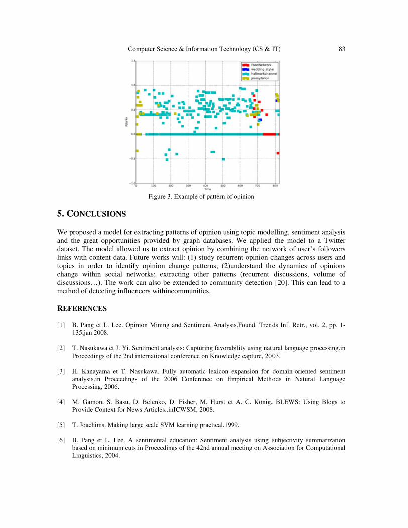
Computer Science & Information Technology (CS & IT) 83
Figure 3. Example of pattern of opinion
5. CONCLUSIONS
We proposed a model for extracting patterns of opinion using topic modelling, sentiment analysis
and the great opportunities provided by graph databases. We applied the model to a Twitter
dataset. The model allowed us to extract opinion by combining the network of user’s followers
links with content data. Future works will: (1) study recurrent opinion changes across users and
topics in order to identify opinion change patterns; (2)understand the dynamics of opinions
change within social networks; extracting other patterns (recurrent discussions, volume of
discussions…). The work can also be extended to community detection [20]. This can lead to a
method of detecting influencers withincommunities.
REFERENCES [1] B. Pang et L. Lee. Opinion Mining and Sentiment Analysis.Found. Trends Inf. Retr., vol. 2, pp. 1-
135,jan 2008.
[2] T. Nasukawa et J. Yi. Sentiment analysis: Capturing favorability using natural language processing.in
Proceedings of the 2nd international conference on Knowledge capture, 2003.
[3] H. Kanayama et T. Nasukawa. Fully automatic lexicon expansion for domain-oriented sentiment
analysis.in Proceedings of the 2006 Conference on Empirical Methods in Natural Language
Processing, 2006.
[4] M. Gamon, S. Basu, D. Belenko, D. Fisher, M. Hurst et A. C. König. BLEWS: Using Blogs to
Provide Context for News Articles..inICWSM, 2008.
[5] T. Joachims. Making large scale SVM learning practical.1999.
[6] B. Pang et L. Lee. A sentimental education: Sentiment analysis using subjectivity summarization
based on minimum cuts.in Proceedings of the 42nd annual meeting on Association for Computational
Linguistics, 2004.

84 Computer Science & Information Technology (CS & IT)
[7] P. D. Turney. Thumbs up or thumbs down?: semantic orientation applied to unsupervised
classification of reviews.inProceedings of the 40th annual meeting on association for computational
linguistics, 2002.
[8] M. Hu et B. Liu. Mining and summarizing customer reviews.InProceedings of the tenth ACM
SIGKDD international conference on Knowledge discovery and data mining, 2004.
[9] S.-M. Kim et E. Hovy. Determining the sentiment of opinions.InProceedings of the 20th international
conference on Computational Linguistics, 2004.
[10] J. M. Wiebe, R. F. Bruce et T. P. OH́ara. Development and Use of a Gold-standard Data Set for
Subjectivity Classifications.InProceedings of the 37th Annual Meeting of the Association for
Computational Linguistics on Computational Linguistics, Stroudsburg, 1999.
[11] A. Agarwal, B. Xie, I. Vovsha, O. Rambow et R. Passonneau. Sentiment Analysis of Twitter
Data.InProceedings of the Workshop on Languages in Social Media, Stroudsburg, 2011.
[12] N. Agarwal et H. Liu. Modeling and data mining in blogosphere.Synthesis lectures on data mining
and knowledge discovery, vol. 1, pp. 1-109, 2009.
[13] H. Yu et V. Hatzivassiloglou. Towards Answering Opinion Questions: Separating Facts from
Opinions and Identifying the Polarity of Opinion Sentences.InProceedings of the 2003 Conference on
Empirical Methods in Natural Language Processing, Stroudsburg, 2003.
[14] V. Hatzivassiloglou et J. M. Wiebe. Effects of Adjective Orientation and Gradability on Sentence
Subjectivity.InProceedings of the 18th Conference on Computational Linguistics - Volume 1,
Stroudsburg, 2000.
[15] L.-W. Ku, H.-W. Ho et H.-H. Chen. Novel Relationship Discovery Using Opinions Mined from the
Web.InProceedings of the 21st National Conference on Artificial Intelligence - Volume 2, Boston,
2006.
[16] V. M. K. Peddinti et P. Chintalapoodi. Domain Adaptation in Sentiment Analysis of
Twitter.InProceedings of the 5th AAAI Conference on Analyzing Microtext, 2011.
[17] T. Hofmann. Probabilistic Latent Semantic Indexing.InProceedings of the 22Nd Annual International
ACM SIGIR Conference on Research and Development in Information Retrieval, New York, NY,
USA, 1999.
[18] D. M. Blei, A. Y. Ng et M. I. Jordan. Latent Dirichlet Allocation.J. Mach. Learn. Res., vol. 3, pp.
993-1022, #mar# 2003.
[19] C. J. Hutto et E. Gilbert. VADER: A Parsimonious Rule-Based Model for Sentiment Analysis of
Social Media Text.InProceedings of the Eighth International Conference on Weblogs and Social
Media, {ICWSM} 2014, Ann Arbor, Michigan, USA, June 1-4, 2014., 2014.
[20] L. Chunshan, C. William K, Y. Yunming, Z. Xiaofeng, C. Dian-Hui et L. Xin. The Author-Topic-
Community model for author interest profiling and community discovery.Knowl. Inf. Syst, vol. 44, n°
%12, pp. 359-383, 2015.

David C. Wyld et al. (Eds) : CCSEIT, AIAP, DMDB, ICBB, CNSA - 2017 pp. 85– 100, 2017. © CS & IT-CSCP 2017 DOI : 10.5121/csit.2017.70609
FINGERPRINT RECOGNITION
ALGORITHM
Farah Dhib Tatar
Department of Electrical Engineering, National school of the studies of engineer of Tunis, Tunisia
ABSTRACT
Biometrics is an emerging field where technology improves our ability to identify a person. The
advantage of biometric identification is that each individual has its own physical characteristics
that cannot be changed, lost or stolen. The use of fingerprinting is today one of the most reliable
technologies on the market to authenticate an individual. This technology is simple to use and
easy to implement. The techniques of fingerprint recognition are numerous and diversified, they
are generally based on generic algorithms and tools for filtering images.
This article proposes a fingerprint recognition chain based on filtering algorithms. The results
are retrieved and validated using Matlab.
KEYWORDS
Fingerprint, Biometrics, Images Processing, Algorithms, Matlab
1. INTRODUCTION
In recent decades, the explosion of information technology and communication networks has significantly increased the need for people to identify themselves. And since security is a natural human need that is becoming increasingly important, reliable identification of people has become a major problem for various applications (border control, access to public places, transport). All these problems have thus led to an increased development of biometric identification techniques. Fingerprint recognition has been known since 1880, thanks to Alphonse Bertillon's research on the identification of recidivists. Our fingerprints are unique, at least on certain points: they are called minutiae, that is, lines, bifurcations, "islands", points and ridge terminations. And then, several studies have been elaborated; so there are several types of algorithms such as HMFA (Histogram-Partitioning, Median-Filtering Fingerprint Recognition Algorithm), an algorithm based on Gaussian filters to minimize the noise existing on the image to be treated [1]; Other studies have focused on improving the comparison phase to ensure rapid authentication [2]. There are also algorithms [3] based on the recognition of the iris, the geoetry of the hand, the face’s geometry ... etc, using generic algorithms.

86 Computer Science & Information Technology (CS & IT)
The performances of these different studies remain variable and depend on several factors (the sensors, the state of the duty, the climate, etc.); For this purpose there exist other studies which were based on optimization tools such as for example the MCS algorithm (MCS: Modified Cuckoo Search) which is an algorithm used as a code optimizer allowing to search for the best distribution of gray levels that maximizes The objective function. [4] In this paper we represent a fingerprint recognition algorithm based on variance calculations and Gabor filtering. We also use Matlab for validation and retrieval of results.
2. COMPLETE CHAIN OF FINGERPRINT RECOGNITION
The proposed fingerprint recognition algorithm consists of two essential parts: pre-processing of the fingerprint image to improve its quality and the extraction of the signature. Pre-processing is a very important phase in the algorithm. Indeed, it makes it possible to improve the image to facilitate the task in the second step and to optimize the processing of the image; the different preprocessing phases are presented in the following figure:
Figure 1. Pre-processing steps
For the extraction of biometric data (the biometric data concerning the fingerprint are the minutiae), the algorithm of the following figure was used.
Figure 2. Extracting signature steps

Computer Science & Information Technology (CS & IT) 87
2.1. Grayscale Transformation
A fingerprint sensor usually returns a color image. For this algorithm, the color planes are not required for processing, so each pixel will be represented on 8 bits (from 0 to 255 gray levels) instead of 24 bits for the color image (RGB or YCrCb ), This step makes it possible to optimize the general appearance of the image and facilitates biometric processing.
2.2. Image normalization
Normalization is used to standardize the intensity values in an image by adjusting the range of gray level values so that they extend in a desired range of values and improve the contrast of the image. The main goal of normalization is to reduce the variance of the gray level value along the ridges to facilitate subsequent processing steps. Normalization is performed locally on each block according to the following steps: Averaging :
(1)
I (i, j) is the value of the pixel (i, j), M is the average value of the image and m, n are the dimensions of the image.
• Variance Calculation :
(2) V is the variance of the image.
• Calculating the value of the normalized gray level of the pixel l (i,j) [13] :
�(�, �) =��� +�� × (�(�, �) − �)��� −�� × (�(�, �) − �)��
� ���(�, �) > ����(�, �) < �
(3)
M0 and V0 are the desired values of the average and variance respectively. Normalization does not change the structure of the image, but it is used to standardize the variation of gray levels.

88 Computer Science & Information Technology (CS & IT)
2.3. Segmentation
In order to eliminate the edges of the image and areas that are too noisy, segmentation is necessary. It is based on the calculation of the variance of gray levels. For this purpose, the image is divided into sub-blocks of (W × W) size’s and for each block the variance according to formula (2) is calculated. Then, the root of the variance of each block is compared with a threshold T, if the value obtained is lower than the threshold, then the corresponding block is considered as the background of the image and will be excluded by the subsequent processing. Otherwise, the block will be considered as the useful part of the image. The selected threshold value is T = 0.1 and the selected block size is W = 16 [7]. This step makes it possible to reduce the size of the useful part of the image and subsequently to optimize the extraction phase of the biometric data. 2.4. Spatial estimation of the directional map We have two steps for a directional map: estimating the orientation and smoothing the directional map. 2.4.1. Orientation estimation:
The directional map defines the local orientation of the striates contained in the impression. The estimation of orientation is a fundamental step in the process of image enhancement based on Gabor's filtering. (figure 3)
Figure 3. Local orientation of a pixel
The associated direction Ѳ (i, j) to a pixel cannot be determined efficiently if it is based solely on the value of the gray level of the pixel. For this purpose, we consider its neighborhood V of size W × W pixels (the considered pixel is the center of the block) and compute the gradients Gx (i, j) along the lines and Gy (i, j) Pixel (i, j) of the neighborhood V according to formulas (4) and (5). For the calculation of the gradients, the SOBEL masks are used as follows:
(4)
(5)

Computer Science & Information Technology (CS & IT) 89
Thus, the local direction in the vicinity V, in the direction of the lines (Vx (i, j)) and in the direction of the columns (Vy (i, j)) is estimated by the following calculation:
(6)
(7)
The estimation of the local orientation in the neighborhood V is Ѳ (i, j) such that:
(8)
2.4.2. Smoothing the Directional Map
Practically, it is possible to have a block so noisy that the directional estimate is completely false. This then causes a very large angular variation between two adjacent blocks. However, a fingerprint has some directional continuity, such a variation between two adjacent blocks is then representative of a bad estimate. To eliminate such discontinuities, a low-pass filter is applied to the directional board. The application of a low pass filter requires that the orientation of the image be converted into a continuous vector field. This vector field has as components x and y respectively defined by:
(9)
(10)
With the two components of the vector obtained, one can apply the Gaussian low pass filter of size WѲ × WѲ defined by:
(11)
(12)
Where G is the Gaussian low pass filter, w is the block size’s. Finally, the local orientation smoothed to the pixel (i, j) is given by:
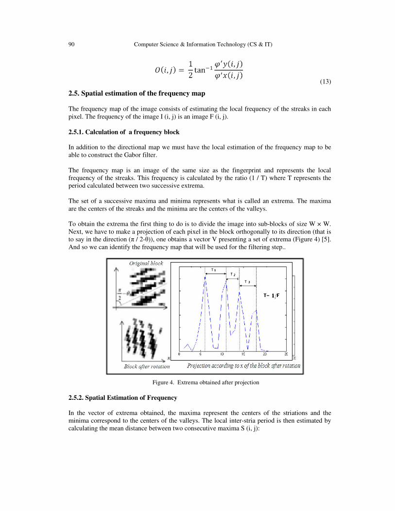
90 Computer Science & Information Technology (CS & IT)
(13)
2.5. Spatial estimation of the frequency map The frequency map of the image consists of estimating the local frequency of the streaks in each pixel. The frequency of the image I (i, j) is an image F (i, j). 2.5.1. Calculation of a frequency block
In addition to the directional map we must have the local estimation of the frequency map to be able to construct the Gabor filter. The frequency map is an image of the same size as the fingerprint and represents the local frequency of the streaks. This frequency is calculated by the ratio (1 / T) where T represents the period calculated between two successive extrema. The set of a successive maxima and minima represents what is called an extrema. The maxima are the centers of the streaks and the minima are the centers of the valleys. To obtain the extrema the first thing to do is to divide the image into sub-blocks of size W × W. Next, we have to make a projection of each pixel in the block orthogonally to its direction (that is to say in the direction (π / 2-θ)), one obtains a vector V presenting a set of extrema (Figure 4) [5]. And so we can identify the frequency map that will be used for the filtering step..
Figure 4. Extrema obtained after projection
2.5.2. Spatial Estimation of Frequency
In the vector of extrema obtained, the maxima represent the centers of the striations and the minima correspond to the centers of the valleys. The local inter-stria period is then estimated by calculating the mean distance between two consecutive maxima S (i, j):

Computer Science & Information Technology (CS & IT) 91
(14)
The maxima Mi and the minima mi are determined by detecting the zero crossing of the derivative of the vector V, which makes it possible to obtain the sequence {M1, m1, ..., Mk, mk, Mk + 1}. If the difference between a maximum Mi and a minimum mi is less than a threshold T then we consider that Mi corresponds to a noise and is eliminated. If the resulting vector contains at least two maxima then the inter-stria period is calculated by the mean of the distances between two consecutive maxima, otherwise the period takes the value of zero. When the estimated period is zero this means that the block contains no streak (background image) or that it is too noisy to reliably estimate the local frequency. The frequency map is a function of the gray level (dark areas = low frequency and light areas = high frequency). 2.6. Gabor Filtering
The principle of filtering is to modify the value of the pixels of an image, generally in order to improve its appearance. In practice, it is a matter of creating a new image using the pixel values of the original image, in order to select in the Fourier domain the set of frequencies that make up the region to be detected. The filter used is the Gabor filter with even symmetry and oriented at 0 degrees (formula 15):
(15)
The values of ��and �� are chosen such that �� = ��. F(i,j) and �� =�� . F(i,j). The values of �� and �� are fixed to be 0.5.
To obtain other orientations, it is sufficient to carry out a rotation of the coordinate axes according to the formula:
(16)
According to the different blocks of the image, the filter can have several favored directions. In this case, the final filter is a sum of basic filters placed in each direction.
The resulting image will be the spatial convolution of the original (normalized) image and one of the base filters in the direction and local frequency from the two directional and frequency maps according to the formula 17:

92 Computer Science & Information Technology (CS & IT)
(17)
with : - E(i,j) is the new value of the pixel (i, j) - O(i,j) and F(i,j) Are the values of the pixels (i, j) of the directional and frequency maps. - � and � Are respectively the length and the width of the block used for the
convolution.
2.7. Image Binarization To allow skeletonization, the image must first be binarized, ie the image in 256 levels of gray that we have at this stage is transformed into a binary image where the black pixels correspond to the streaks and The white pixels to the valleys. There are many techniques of image binarization [8], we chose to use a simple and effective thresholding method. To perform this processing, the value of each pixel P(x,y) is compared with a threshold M and if this value is greater than the threshold the pixel takes the value of one (black), else it takes the value of zero (white). 2.8. Skeletonization of the image To facilitate extraction of minutiae the image must be skeletonized: a sequence of morphological erosion operations will reduce the thickness of the striations until the latter is equal to one pixel while maintaining the connectivity of the striations ( That is to say that the continuity of the striaes must be respected, holes must not be inserted). We used the Rosenfeld algorithm [9] for its simplicity and because it is well adopted at the hardware implementation as it has a reduced computation time compared to the other algorithms. [10] The use of the Rosenfeld algorithm allows to optimize the overall processing time 2.9. Detection of minutiae The method used is the Crossing Number (CN) [5]. It is the most used method for its simplicity. One must have as input a skeletonized image. This must have 0 for a white pixel and 1 for a black pixel. The minutiae are extracted by examining the local neighborhood of each pixel in the image of the fingerprint using a connectivity of 8 neighbors (window 3 × 3) (figure 5)
Figure 5. The different representations of the skeletons
The value of the CN is calculated according to formula 18.

Computer Science & Information Technology (CS & IT) 93
(18)
Thus, for a pixel P belonging to a streak (that is to say of value 1), the CN can take five values (figure 6):
• CN(P) = 0 : It is an isolated pixel, we do not take into account it because even if this type of minutia exists, it is very rare and in the general case it is due to a noise residue.
• CN(P) = 1 : It is a candidate for a termination • CN(P) = 2 : This is the most common case, it is a pixel that is on a streak, there are no
minutiae in this case • CN(P) = 3 : A triple bifurcation candidate • CN(P) = 4 : A quadruple bifurcation, this type is quite rare and it is probably due to noise.
Figure 6. Examples of determining the type of minutiae according to CN The detection of minutiae thus causes the presence of a very large number of false minutiae. An additional processing is therefore necessary to eliminate the maximum of the detected false minutiae. 2.10. Elimination of false minutiae This step will make it possible to have at its end the true minutiae that will serve to define the characteristic vector of the imprint. An algorithm [5] adapted to the treatment carried out previously was used. This algorithm is based on empirical results [8] based on the fact that the distance between two neighboring minutiae is always greater than a certain threshold. Indeed, practically it is extremely rare to find two real minutiae very close, on the other hand one almost always a local concentration of several false minutiae. When eliminating false minutiae, we have to traverse the coding image of CN by looking for the values of the pixels of values CN = 1 or CN = 3 each time because we are only interested in these Types of minutiae that are most frequent and that leads to other forms of minutiae.
P1 P2 P3
P8 P P4
P7 P6 P5
!�(") = #�$|"� − "�&#|'�(#
With: )8 = )0), ∈ .0,10

94 Computer Science & Information Technology (CS & IT)
2.10.1. Treatment of detected terminations
When a candidate point T (Tx, Ty) for the termination title (CN = 1) is found, it is first checked whether it is at the edge of the image, since most of the false endings are caused by The edge of the image. This allows the elimination of many false terminations as the lines of the skeleton image stop at the edge of the image thus creating erroneous terminations. Moreover, the segmentation of the image made it possible to determine the unnecessary part considered as background of the image. This part will be used in this phase. Indeed, if a candidate T (Tx, Ty) for a termination is in a block adjacent to a block belonging to the background of the image, it will be considered as a false termination and will therefore be eliminated. For the remaining terminations, one begins from the position of the candidate T (Tx, Ty) to traverse the streak of which he belongs over a maximum distance K1 until reaching the point A (d = TA ≤ K1). Here we have two cases:
• d < K1 and CN(A) = 3 : A bifurcation occurs before reaching the maximum distance. One is in the case of a parasitic branch, then the point T (Tx, Ty) and the bifurcation A encountered are considered as false minutiae and must be eliminated from the list of minutiae. To more understand this case, we can examine the example of figure 7 where the points T and A successively represent a true termination and a true bifurcation; K1 is the mean inter-streaks distance. If we start from point T, then we must not encounter point A (CN = 3) unless we travel at least the distance d ≥ K1; otherwise means we meet a bifurcation between two successive streaks (d < K1): It is then a parasitic branch (false branch or noise) and the points T and A will therefore be considered as false minutiae.
Figure 7. Example of detecting a bifurcation
• d < K1 and CN(A) = 1 : Another termination is encountered before reaching the maximum distance. In the case of a short segment, the point T (Tx, Ty) and the termination encountered are considered as false terminations.
In all other cases, the termination T (Tx, Ty) will be validated. The distance K1 is the average inter-streak distance, it is taken such that K1= 9 pixels [6].

Computer Science & Information Technology (CS & IT) 95
2.10.2. Treatment of detected bifurcations
When a candidate point B for the title of a bifurcation is detected (CN (B) = 3), the three striations associated with it are traced over a maximum distance K1 until three points A1, A2 and A3. (figure 7).
Figure 8. Course of the streaks associated with a bifurcation
Several cases can occur and they are processed in the following order:
• d1<K1, d2 <K1 and d3 <K1 : The circular area with center B and radius K1 contains at least four minutiae (points A1, A2, A3 and B) and which are placed in a radius smaller than the mean inter- streaks distance. We are thus in the case where we find minutiae between two successive streaks, which contrasts with the general tendency of presence of minutiae. We then consider that we are in a very noisy zone (large grouping) and that B is a false bifurcation.
• CN(A1)=1 or CN(A2)=1 or CV(A3) = 1 : At least one of the striae leads to a termination.
And since d ≤ K1 (the path is made over a maximum distance K1), this means that we are in the case of a bifurcation witch one of the branches leads to a termination before reaching the mean inter- streaks distance : In this case both of the detected termination and bifurcation are invalid and are considered to be false minutiae. Figure 9 illustrates this case: point B 1 is followed by a false termination (point A1) and therefore not validated while The point B2 represents a true bifurcation.
.
Figure 9. The case of a false bifurcation
• A1=A2 or A1=A3 or A2=A3 : Two of the striaes lead to the same point. We are in the case of an island, the point B and the bifurcation reached are not validated since, by definition, the bifurcation represents a branching of a single streak into two other streaks. Figure 10 shows the difference between the two cases.

96 Computer Science & Information Technology (CS & IT)
Figure 10. The difference between a true bifurcation and an island
In all other cases the point B is validated as a true bifurcation [6]. 2.11. Vector signature
The signature vector is a file containing useful information for the comparison of the two signatures. Our recognition system is a verification system, that is, it consists in confirming or denying the identity of a person (am I the one I claim to be) in relation to a reference record . One distinguishes then two operations: the recording and the verification. During registration, the signature 12 extracted from the fingerprint is stored in memory. During the verification the user’s signature 13 is compared with 12. Of course these two signatures will never be strictly identical because the impression will never be acquired in a similar way (speed, dust, pressure) and localized distortions (elasticity of the skin) will appear. The authentication of the person then consists in calculating the degree of similarity between the two signatures 12 and 13. This quantified similarity is then compared with a threshold defined in advance according to the chosen application to determine whether or not the person is the right one. Usually the recognition algorithms try to estimate the transformation T to obtain 12 from 13 (Formula 19).
4�5�5678 = �. 4cos = − sin= 0sin = cos= 00 0 �&@8 . A
BC6D + 4∆�∆�= 8
(19)
The parameters (�, ∆�, ∆� , =) characterize the distortion caused by the acquisition:
• k is a constant scaling factor. It is generally considered to be equal to 1 when the images come from the same sensor but its estimation may be necessary in the case of two sets obtained by two different acquisition means ([11]).
• ∆� and ∆� define the translation in x and y of the position of the center of the image.

Computer Science & Information Technology (CS & IT) 97
• α describe the difference in orientation between the two signatures.
In our case it is assumed that the finger always moves in the same direction, even if using a specific system to force the user, so one does not have to take into account the rotation parameter (= =0).
The transformation to the two signatures will therefore be according to the formula 20 :
4B2C2628 = 4B3C3638 + 4∆�∆�0 8 (20)
Once we have done this transformation, we now have two signatures with centers, so the next step is to determine the number of minutiae that is superimposed according to the following two conditions:
• The two minutes are of the same type: F2 =F3. • The characteristic directions of the blocks containing the minutiae are such that: Gsin(62 −63 )G < sin10° [12]
The last step consists in computing the number N of the superimposed minutiae (to ∆ near) and then comparing this number with a threshold M chosen according to the recognition system, if N
≥ M on is the case of the two signatures combined, otherwise No one will be recognized and the two signatures will be considered different.
3. RESULT AND DISCUSSION MATLAB was used to develop and validate this code, from the preliminary processing phase of the image to the extraction of the signature vector, which allows us to identify and compare the different fingerprints. Then we validated our algorithm with respect to a database containing a hundred of the untreated images. The two following figures represent respectively the phase of elimination of the false minutiae as well as the extraction of the signature vector.
Figure 11. Result of the elimination of false minutiae stage

98 Computer Science & Information Technology (CS & IT)
The signature vector: This file is used in the matching phase. At the end of this phase it can be concluded whether it is indeed the desired signature or not with an acceptable margin of error.
Figure 12. Illustration of the margins of error associated with the signature
By comparing the signature vector of the captured image with those that are recorded in the database the system concludes then whether or not the person is recognized and decides the permission or inhibition of access. The originality of this method is manifested in the reduction of the useful information comprised in the signature vector: if we locate the true and necessary minutiae for the comparison phase, we will have to compare fewer points while keeping the specific characteristics of each fingerprint. Although the pre-processing phase of the image allows us to improve the general appearance of each fingerprint and then facilitates the detection of minutiae; The most important phase is the elimination of false minutiae. Consider, for example, the case illustrated in Figure 13:
Figure 13. Identification of the phase of elimination of false minutiae
If a comparison procedure is used based on all detected minutiae; We have to compare 36 points (22 bifurcations and 14 endings), of which 23 points represent false minutiae (16 bifurcations and 7 endings); The error rate is therefore 63.8%, whereas after the elimination of the false minutiae, only 12 points (5 bifurcations and 7 endings) will be compared with an error rate that does not

Computer Science & Information Technology (CS & IT) 99
exceed 1% and although we have eliminated a significant number of minutiae detected, the techniques used and explained above allow us to keep the information useful, necessary and sufficient to ensure comparison between the captured fingerprint and the one that is registered in our database. In addition to reducing the error rate, reducing the number of points (minutiae) compared, allows us to save a lot of time during the comparison phase (for the previous example: compare 12 points instead of 36) and subsequently improve overall system performance and even facilitate the implementation task on a hardware platform.
4. CONCLUSION
The results obtained are directly linked to two main criteria: the captured image quality and the processor used to process the images. There are several types of sensors used for image acquisition the most used sensors in the market are the CMOS sensors since they allow to reduce the overall price of cameras, since they contain all the elements necessary for the composition cameras. Concerning the implementation of code there are also several types of processors that can be used ranging from those provided by companies specialized in embedded manufacturing such as Altera, Xilinx, Texas Instrument ... etc. Or "free" processors such as Raspberry Pi, Beaglebone, Arduino and others. The performance of the software and the code remains strongly dependent on these two steps and varies mainly according to the types of processors used for the processing of the image. REFERENCES
[1] Ayyüce M. Kizrak , Figen Özen “A new median filter based fingerprint recognition algorithm”, Haliç
University, Electronics and Communications Engineering Department, Suracevizler St. No.29, Bomonti, sisli, Istanbul 34363, Turkey, Elsevier 2011.
[2] Christel-Loïc TISSE, Lionel MARTIN, Lionel TORRES et Michel ROBERT, « Système automatique
de reconnaissance d’empreintes digitales. Sécurisation de l’authentification sur carte à puce »,Advanced System Technology Laboratory STMicroelectronics – ZI Rousset – 13106 Rousset, France, Université de Montpellier, UMR 5506, L.I.R.M.M.161, rue Ada -34392 Montpellier, France.
[3] Pratibha Sukhija, Sunny Behal and Pritpal Singh,” Face Recognition System Using Genetic
Algorithm”, International Conference on Computational Modeling and Security (CMS 2016). [4] Subba Reddy Borra, G. Jagadeeswar Reddyb and E. Sreenivasa Reddyc, “An Efficient Fingerprint
Enhancement Technique using Wave Atom Transform and MCS Algorithm”, Twelfth International Multi-Conference on Information Processing-2016 (IMCIP-2016)
[5] W. Zhao, R. Chellappa, P.J. Phillips and A.Rosenfeld, Face recognition: A literature survey, ACM
Computing Surveys (CSUR), Volume 35, Issue 4, December 2009. [6] G.O. Williams, Iris Recognition Technology , IEEE Aerospace and Electronics Systems Magazine,
Volume 12, Issue 4, pp. 23 -29, April 2003. [7] A.K. Jain, S. Prabhakar and S. Pankanti, "Twin Test: On Discriminability of Fingerprints", Proc. 3rd
International Conference on Audio- and Video-Based Person Authentication,, pp. 211-216, Sweden, June 6-8, 2007.

100 Computer Science & Information Technology (CS & IT)
[8] http://www.referencement-internet-web.com/15777-Passeport-biometrique-empreintes-digitales-numerisees. html
[9] http://www.lextronic.fr/P2242-module-oem-biometrique-sfm3020-op.html [10] http://www.agent-de-securite.be/biometrie/securite_biometrique.html [11] A.M. Bazen and S.H. Gerez, "Directional Field Computation for Fingerprints Based on the Principal
Component Analysis of Local Gradients", in Proceedings of ProRISC2000, 11th Annual Workshop on Circuits, Systems and Signal Processing, Veldhoven, Netherland, November 2009..
[12] T. Aach, I. Stuke, C. Mota and E. Barth, "Estimation of Multiple Local Orientations in Image
Signals", IEEE International Conference on Acoustics, Speech and Signal Processing, Quebec, 2010. [13] http://focus.ti.com/docs/toolsw/folders/print/tmdsdsk6416.html
AUTHOR Farah Dhib Tatar Specialty: Electrical Engineering (Embedded Systems) Education: o 2010: Engineering Degree from sfax College of Engineering, ENIS, Tunisia o 2012: Master degree from Sfax College of engineering, ENIS, Tunisia o In progress: Ph.D. degree from Tunis College of engineering, ENIT, Tunisia Experience: o 2010-2016: College of Higher Studies and Technologies ISET, Tunisia

David C. Wyld et al. (Eds) : CCSEIT, AIAP, DMDB, ICBB, CNSA - 2017
pp. 101– 111, 2017. © CS & IT-CSCP 2017 DOI : 10.5121/csit.2017.70610
IMPROVEMENT OF EMAIL THREATS
DETECTION BY USER TRAINING
V.Bernard, P-Y.Cousin, A.Lefaillet, M.Mugaruka, C.Raibaud
Undergraduate Students
ECE Paris School of Engineering
Paris, France
ABSTRACT
With the generalization of mobile communication systems, solicitations of all kinds in the form
of messages and emails are received by users with increasing proportion of malicious ones.
They are customized to pass anti-spam filters and ask the person to click or to open the joined
dangerous attachment. Current filters are very inefficient against spear phishing emails. It is
proposed to improve the existing filters by taking advantage of user own analysis and feedback
to detect all kinds of phishing emails. The method rests upon an interface displaying different
warnings to receivers. Analysis shows that users trust their first impression and are often lead
to ignore warnings flagged by proposed new interactive system.
KEYWORDS
Phishing, Spam, Human Sensors, User-based Paper
1. INTRODUCTION
The tremendous increase of information traffic on the various available supports has correlatively
augmented considerably the flow of useless and even dangerous information, up to the point that,
overall, the value of global information content is proportionally decreasing. Mail credibility
becomes difficult to discern because of growing useless “information” polluting inboxes. Much
worse, there is in parallel a trend difficult to stop, where more and more emails are targeted by
computer attacks [1] for stealing information and/or ransoming them, damaging infrastructure or
creating botnets. Despite constant surveillance from dedicated watching sites and accelerated up-
to-date production of protecting software against viruses and malware, these attacks are now
adaptively developed according to the target, the attacker and its final goal [2].
Simplest case corresponds to Phishing with a good-looking email asking user to click or reply
[3,4]. Spear-Phishing email is customized to pass anti-spam filters and targeted to a small number
of users. Pharming is a Phishing improved version where targeted legitimate site is duplicated in
user browser address bar by poisoning the victim DNS server and remapping the target website
domain onto pharming site IP address. Least visible and most dangerous Advanced Persistent
Threat (APT) attacks are used to extract sensitive data and to create backdoors in user system for
later access.

102 Computer Science & Information Technology (CS & IT)
Despite good anti-techniques such as content-based [5-7] and behavior-based [8-11] ones, the
attacks are still a serious problem because phishes continually change their ways to defeat the
anti-phishing techniques. Also, most existing emails filtering approaches are static easy to defeat
by modifying emails content and link strings. To counter Phishing attacks, existing approaches
are mostly based on technical tools [1218], or sometimes in combination with a human sensor
[19-20]. Today filters inefficiency against spear-phishing emails constitute a weak point of
entrance into supposedly “protected” private emails. In the following the possibility to improve
the situation is discussed by implying user participation with adequate training to recognize
attacks more easily.
Technical approaches [21-24] attempt to automatically identify fraudulent messages and either
discard them immediately or warn the users of their potentially harmful nature. Machine Learning
is a good example of technical approach used as a solution to counter phishing attacks [5,2527].
Test of different algorithms to determine which one has best efficiency gives a value around 90%
for all of them [7,28]. However, this is an inappropriate rate given the total volume of phishing
attacks. Present approach is different as it combines a technical tool with human interaction, with
the intention to determine how much more efficient is user implication for spear phishing
detection. Some solutions combining technical tool and human sensor have been tried. For
instance, when addon browser BAYESHIELD [29] detects a potential phishing website, it
displays a blocking pop-up asking users to use tool Analyzer part in order to detect whether the
website is legitimate or not. The software also asks users different questions organized in three
categories: a) easy to understand (no complicated terms), b) easy to answer (the questions do not
strain their cognitive load), c) educative (users will learn to detect phishing without the help of
any tool). The results are interesting as the tool helps users to distinguish legitimate websites from
fake ones. Their feedback is very positive as they appreciated the tool support in their decision.
Spear-phishing attacks can be executed on any social media platform. The content of sent
messages is usually designed to be interesting for the recipients [3]: it can be based on their
hobbies, their personal information, profession, ... Most reviewed studies about phishing count the
number of users who filled a form with personal information, credentials or banking information
to distinguish users falling into the phishing from users recognizing it. This approach is not
pertinent here.
Spear-Phishing containing an APT can infect a system by just clicking on a link or on the
attachment. The exploitation is triggered immediately after the user interaction, so it is very
important that the user can detect a Spear-Phishing email and do not click on the links inside nor
on the attachments. Moreover, if detection rules between Phishing and SpearPhishing differ, they
share a common basis but Spear-Phishing is designed to bypass anti-phishing systems and to be
very discreet as it is the first step of a big and elaborated attack [4].
The solution proposed in the following is based on the same principle as BAYESHIELD, with the
difference that instead of focusing on website detection, attention is focused on email spear-
phishing detection and the tool is tested in real conditions.

Computer Science & Information Technology (CS & IT) 103
2. SYSTEM DESIGN
2.1. The Add-On
Here a THUNDERBIRD (an email application) add-on is developed reacting to a potential threat
identification. The addon has been tested on THUNDERBIRD 45.0.x. When it occurs, the
receiver must be warned to think about the danger it can be exposed to. For the add-on, a window
appears with questions about elements of the received email, like attachment, link, failure in
sender identification.
The asked questions are easy to understand. If the email contains a link, the user is warned about
its existence. He is asked if the link really redirect towards what it announced it would do and
how he can check it. In case the email contains some attachment, the user is asked if he expected
to receive a file and is warned about it. The asked questions are easy to understand. If the email
contains a link, the user is warned about its existence. He is asked if the link really redirect
towards what it announced it would do and how he can check it. In case the email contains some
attachment, the user is asked if he expected to receive a file and is warned about it. Finally, in
email header, the security SPF Test can assert whether the domain name is real or usurped. If the
SPF Fail is not succeeding, which means that it is potentially usurped or is not just recognized,
the user is warned that the email may be potentially malicious.
Attachment is detected by looking at attachment part into email header. To detect the link, one
just search on the raw text, without html tags, the string “http” or “www”. Then the user is
supposed to make the appropriate decision. There are different possibilities. First, the email is
suspicious and the user discovers it. He reports it as a spam in order to improve the Bayesian
filter which decides if an email is dangerous or not. Second, and it is why it is chosen to make a
send-email window appear for warning the IT department about the potential danger and letting it
take appropriate measures. If the user, despite the warning, still decides to trust the email, it is at
his own risk and the warning existence does not change the result. Unfortunately, a legitimate
email can make the add-on react. Then, the user can encounter a problem. If the user uses the
program for too long, his attention can be reduced. In this case, the user will just throw the emails
to spam, like if they were malicious ones. This is probably the most dangerous habit the user can
have. But if he keeps his attention focused and takes the time to verify if the emails are legitimate,
everything is good.
2.2. Mailing
For the mailings, SEES software and POSTFIX on a Kali Linux VIRTUALBOX have been used.
POSTFIX has been configured to use one of the domains we bought.
SEES software allows individually sending emails the sender email address, the sender name and
the other usual mailing fields of which can be directly set. The software does not allow any
individual customization in the body. For logistic reasons, the number of hits per link per
population has also been counted. In the experiment performed on site at ECE Paris School of
Engineering, the sent emails are not considered as spams by the school webmail (office 365) or
by any other email client.

104 Computer Science & Information Technology (CS & IT)
3. USER-STUDY METHODOLOGY
The goals of the study are:
1) to compare the click-rate on Phishing and Spear-Phishing mailings between a user group
supposedly sensitized to security issues and a nonsensitized one.
2) to compare the click-rate with and without proposed tool.
3) to determine if the tool has helped the users in detecting the junk emails they received.
4) to determine if and how many users identify malicious email.
The developed add-on asks questions to the users on some emails that the email server does not
know how to classify: i.e. it is not sure whether the email is legitimate or not.
Thirty participants have been recruited as the testing population to install and use proposed add-
on. They were told that the tool was in use to prove that users should be included in junk or
phishing detection. Questions have been asked to them on potential dubious points that should
help them determine if those emails are illegitimate, in exchange to a small reward for their
participation. The control population has been divided into three main groups. The first group
counts 86 users who belong to Engineering School. Most of them have basic knowledge on
computer security. The second and third groups belong to Business and Management Schools.
These users are supposedly not sensitized to computer security. No group was aware of the study.
All participants are under 25 years old and undergraduates.
A total of four phishing or spear-phishing emails have been sent so as to have a consistent set of
data. The goal of these emails was to have the participants click on a link provided in it. The
number of clicks on the links are collected by using a bit.ly account. Each time different links
have been used by email: one by school for the control population and one for the testers.
For phases 1 and 2, to make emails look more credible, a domain name similar to chosen “victim”
organization has been taken, and an email has been sent from a non-existing person in the
company ([email protected] for instance). To make everything look normal, a failure in
SMTP protocol, allowing to send an email from any fake or real sender, has been exploited.
Protections against this failure exist but must be implemented by the domain you spoof. For legal
reasons, permission has been asked to domain’s owner or used nonexistent one for the other
phases.
Phishing emails differ according to the school for legal reasons. A validation has been asked for
each email sent with an usurped identity. Four tests have been conducted corresponding to
different users’ behavioral aspects.
3.1 Test Campaign 1
An email has been sent to all (students) populations informing them that their report is available
on the online grade platform. Some of the schools do not use such system but it was anticipated
that users would click anyway without checking for basic signs of phishing (wrong URL,

Computer Science & Information Technology (CS & IT) 105
unknown sender, breaking the habit) because grades are a highly sensitive subject in this period
and many students fear failing their courses. The email was sent from an unknown sender (who
sounds like a real staff working there) with a fake email address.
3.2 Test Campaign 2
Here, the email differs depending on the targeted school. For the first one, it was an email about a
change in their timetable. For the other ones, it was an email informing the user that a tutorial
about the use of the printers were available. It was sent from a legitimate address.
3.3 Test Campaign 3
For third phase, a commercial ad was sent by email. Since the first semester just ended, the
“shop” was offering 20% off the alcohol. The email invited users to click on a link to discover the
shops participating to the operation. The clues for the users to determine that it was not legitimate
were: the obfuscated link, no possibility to unsubscribe the newsletter (it is mandatory in the EU),
the lack of any shop with this name and finally, that they did not subscribe to any information of
this kind.
3.4 Test Campaign 4
In last test, an email was sent informing the students they had submitted their work on the school
moodle. Of course, they did not. The course did not even exist. The sender address was unrelated
to the school but the expedient name sounds legitimate, i.e. its name is “Name of the school” and
its address [email protected] . This phase allows verify what the user checks when they receive
shady emails.
4. RESULTS
4.1 Global Results
The population sizes are: 86 for School 1 (S1- Engineering School), 60 for School 2 (S2-
Business and Management School) and 220 for School 3 (S3- Business and Management School).
To analyze the results, the following “global click response” (GCR) coefficient γ given by (1) will
be used
γ = 102 χ.ν (1)
where χ = {Click Number/Number of Clicking Persons} and ν = {Number of Clicking
Persons/Tested Population Number}. This coefficient is grouping two different elements {the
number of clickers in a population, the number of clicks per clicking person} together, depending
respectively on tested population number and individual response of tested groups. Even if χ and
ν are generally independently required for specific study, GCR γ is for present discussion
representative of tested population response. The fact that γ > 102 because χ >1 is here useful as it
enhances the difference between the different tested groups. The most successful tests are first
and last ones. The first test corresponds to the most advanced attack and the hardest to detect. The
last one was testing user habits and awareness level. There is no data for S2 because authorization

106 Computer Science & Information Technology (CS & IT)
was not obtained from school administration. S1 students clicked the less on proposed links.
During first test campaign, a huge spike for S2 students reaches around 360%, see Fig. 1.
Figure 1: GCR λ per Population per Campaign Cj
S3 students clicked about 170% and S1 students around 110%. Testers performed worse, about
130%. For tests 2 and 3, results are quite similar for every population. For test 2, the average click
rate is around 15% and for test 3 about 5%, except for S2, with a click rate of 14%. None of the
testers clicked on this mail. For the last test campaign, the click rate is about 44% for S1, 50% for
S3 and 21% for volunteer population.
Relevance of proposed tool can be analyzed on Fig. 2 It compares the ratio clicks/control
population with the clicks/test population. It brings to light that the curves are quite similar and
follow the same tendencies. One can distinguish for test campaign 4 a small difference. Control
population clicked around 40% whereas testers did 20%.
Figure 2: Evolution of GCR λ for Control and Recruited Population.
4.2 Results for Test Campaigns 1 and 4
As campaigns 2 and 3 had a very low click rate, the daily analysis was dismissed. The
percentages presented in this section are calculated as: ���������� ������
��������������∗ 100 (2)
4.2.1 First Campaign
During this campaign, the main objective was to create an email the users would crave to read
and click on associated link. As it was the end of the semester, the created email was announcing

Computer Science & Information Technology (CS & IT) 107
that the results were available on the grade platform. A particular attention has been taken to
every detail, name, template, etc. The fake email was based on a similar email sent by the
administration of the schools two years before.
Figure 3: First Test GCR λ per Day.
There was no similar email sent since then. Fig. 3 shows that S3 massively click on the link
(around 160%) the first day, but not after. About 70% of S1 clicks are the first day. There is about
10% of S1 clicks on day 2, 3 and 4. S2 and tester clicks are around 45% the first day and stabilize
for S2 the second day and quickly drop to zero during day 3 and 4. For testers, click percentage
stabilizes around 15% until day 6 and then drops to around 3%.
4.2.2 Fourth Campaign
For last test, a new phishing email was sent but this time, with more intriguing features. The
designed was basic and the sender address had nothing to do with something remotely legitimate.
If the user read the email address, he directly understands the email is a setup. The goal was to
determine if users check for basic signs of spam in an email.
Fig. 4 shows that, S1 click on the link the first day but not after. About 80% of tester clicks are
the first day. There is about 20% tester clicks on day 2 and none after. S3’s clicks are about 60%
the first day, it quickly stabilizes around 15% on day 2 and 3. It drops to roughly 10% on day 4.
Figure 4: Fourth Test GCR λ per Day

108 Computer Science & Information Technology (CS & IT)
5. ANALYSIS
To validate them, survey covering all previously sent emails was sent to all participants asking
why they trusted the emails or not, or why they thought it was legitimate.
1)- It cannot be as certain from reported results that there is no statistically convincing data
confirming the improvement of phishing detection with proposed tool.
2)- Many users rely on the pair {sender name/subject} to determine whether the email they
received is legitimate or not. This is further reinforced by the fourth test phase results. The sender
email address was off. It did not even look like something legitimate. However, one still observed
a 40~50% click rate on the links. To further check this hypothesis, the email sent was about a
homework the students submitted online, but in a subject outside their cursus, after it was checked
they did not submit a homework in any subject at all recently. This result can be explained by the
fact that whether on a PC or a mobile phone, it is the two first information available. Furthermore,
on a mobile, they are generally the only one available, the email address being usually hidden.
3)- There is no real discrepancy between supposedly sensitized and non-sensitized populations
ones. They all clicked in similar proportions during the different test campaigns (difference <5%).
It can be seen that test population did not click on the links at all during third test whereas the
other populations had non-null click rate.
In first test campaign, the click/population number ratio is above 1. The result is explained by
users’ frustration not to get the promised information and clicking again in believing it was an
error. The link redirected them to the school extranet that they, subconsciously, consider as safe
and legitimate. Others clicked in the following days thinking the information would be posted
later. It is possible that the greater is the ratio, the more difficulty it indicates for the “victims” to
spot that it was a spear-phishing.
4)-The high score of first test campaign comes from arousal of students’ curiosity and from their
need for reassurance against a possible catch-up exam. Therefore, when seeing the email, they
thought it was legitimate and did not further check for a phishing. Even those with the add-on did
not pay attention to the alert.
The spear-phishing was a high quality one: the message, subject, sending timing and sender were
conceived to catch the receiver. A technical fault was exploited to use the domain name of their
school and be shown as legitimate. Results are similar to previous studies with trained users [30]
The family and given names of sender person were like a real staff member. Students’ feedback
shows that they thought they knew the created person.
5)-This is further reinforced in the third test during which few clicks are counted: 4% for S3, 7%
for S2, 4% for S1, and 0% for recruited population. It was sent like a normal phishing would be,
which can explain their improved awareness. Also, the subject might not be of interest for
everyone (alcohol price reduction).
The same can be said for the second test (email about their timetables and printers), the emails
had an informative objective and did not present any priority need. Many users said that they
deleted it without looking at it like they usually do for this kind of email. When asked about its
legitimacy, they answered that it seemed legitimate but it did not interest them. Therefore, they

Computer Science & Information Technology (CS & IT) 109
made a mistake in their analysis but it was a benign one because email deletion protected them
from possible harm.
6)- Furthermore, many users have bad IT habits. They click on the links present in the emails
instead of accessing the website by their own means. They do not pay attention to details (sender
email, mistakes, sending legitimacy). When comparing the number of testers to the amount of
feedbacks received from the add-on, it appears that users did not feel the need to use proposed
extension because they did not see problems in the emails or just did not pay attention to pop-up
[23,24]. When comparing present study to other ones, it was supposed that the pop-up did not
block the user enough and it could easily be closed. For technical reasons, the pop-up was only
monochrome which might not have attracted enough user attention. Also its repetitive aspect
probably contributed to the low amount of feedback from the add-on.
6. CONCLUSIONS
When compared to other similar ones, present study has been conducted in life conditions and not
in artificial environment. Though more realistic, this might have had a negative impact on present
results. The objective of the study was to set up a technical solution involving user interaction in
spam and phishing more effective detection. The intention was to demonstrate that user inclusion
in the fight (wrestling) against Phishing was more effective than just with the machine. After
several test campaigns, two observations can be highlighted. First, within the studied framework,
the results show that proposed tool does not always improve Phishing detection. Aside inherent
limitations of proposed method, the homogeneous education level of test populations could
introduce some bias in the results. For instance, some related to many users’ bad IT habits, when
they base themselves on the combination {sender name/subject} to determine if received email is
justifiable or not, without paying attention to elements typically present in impish messages, etc.
This would suggest that there is no “universal” best response for user-technical tool collaboration
which is depending on both mail subject and warnings nature and ergonomic presentation in tool
display. This population sensitivity problem will be considered elsewhere. In particular
circumstances, the use of purely technical solution is more efficient than hybrid one including
user interaction will be analyzed, because they correspond to situations where user risks to deliver
bad information to the tool (for example for messages considered as phishing ones by the tool but
considered as legitimate by the user).
ACKNOWLEDGEMENTS
The authors are very much indebted to ECE Paris School of Engineering for having provided the
necessary setup within which the study has been developed, to Drs M. Kadiri and V. Nuzzo for
advices and guidance during the project, Antoine Joly for his proof-reading, and to Pr. M.
Cotsaftis for help in preparation of the manuscript.
REFERENCES [1] The number of detected phishing attacks has increased from 170000 in 2005 to 440000 in 2009
[2] D. Gudkova, M. Vergelis, N. Demidova : Spam and Phishing in Q3 Securelist, 2016. Spammers and
fraudsters are now more interested to make their email contents look as normal as possible, as if they
believed a significant proportion of users have mastered the basics of Internet security and can spot a
fake threat

110 Computer Science & Information Technology (CS & IT)
[3] J. Hong : The Current State of Phishing Attacks, Comm.of the ACM, 55(1), pp.74–81, 2012
[4] L. James : Phishing Exposed. Syngress, 2005
[5] I. Fette, N. Sadeh, A. Tomasic : Learning to Detect Phishing Emails, Proc. 16th Intern. Conf. on
World Wide Web (WWW’07), Alberta, Canada, pp.649–656, ACM, 2007
[6] M. Chandrasekaran, K. Narayanan, S. Upadhyaya : Phishing Email Detection Based on Structural
Properties, NYS Cyber Security Conference, 2006
[7] S. Abu-Nimeh, D. Nappa, X. Wang, S. Nair : A Comparison of Machine Learning Techniques for
Phishing Detection, Proc. Anti-phishing Working Groups, 2nd Annual ECRIME Researchers
Summit, pp.60–69, New York, NY, USA, ACM, 2007.
[8] J. Zhang, Z. Du, W. Liu : A Behaviour-based Detection Approach to Mass-Mailing Host, Proc.6th
Intern. Conf. on Machine Learning and Cybernetics, Vol.4, pp.2140-2144, 2007
[9] F. Toolan, J. Carthy : Feature Selection for Spam and Phishing Detection, Proc. ECRIME
Researchers Summit, pp.1-12, 2010
[10] N.A. Syed, N. Feamster, A. Gray : Learning To Predict Bad Behaviour, NIPS 2007 Workshop on
Machine Learning in Adversarial Environments for Computer Security, 2008.
[11] I.R.A. Hamid, J. Abawajy, TH. Kim : Using Feature Selection and Classification Scheme for
Automating Phishing Email Detection, Studies in Informatics and Control, Vol.22 (1), pp.61-70, 2013
[12] C. Ludl, S. McAllister, E. Kirda, C. Kruegel : On the Effectiveness of Techniques to Detect Phishing
Sites, Detection of Intrusions and Malware, and Vulnerability Assessment, pp.20–39, Springer, 2007
[13] Y. Zhang, J.I. Hong, L.F. Cranor : CANTINA: a Content-based Approach to Detecting Phishing Web
Sites, Proc. 16th International Conference on World Wide Web (WWW’07), Alberta, Canada,
pp.639– 648, ACM, May 2007
[14] M. Wu : Fighting Phishing at the User Interface, PhD Thesis, Computer Science and Engineering,
MIT, 2006
[15] S. Garera, N. Provos, M. Chew, A.D. Rubin : A Framework for Detection and Measurement of
Phishing Attacks, Proc. 5th ACM Workshop on Recurring Malcode, WORM 07, ACM, New York,
NY,‟ USA, pp.1-8, 2007
[16] C. Whittaker, B. Ryner, M. Nazif : Large Scale Automatic Classification of Phishing Pages, Proc.
17th Annual Network and Distributed System Security Symposium, NDSS 10, San Diego, CA, USA,
2010 ‟
[17] R.B. Basnet, A.H. Sung, Q. Liu : Rule Based Phishing Attack Detection, Proc. Int. Conf. Security and
Management, SAM11, Las Vegas, NV, USA, 2011
[18] M. Cova, C. Kuregel, G. Vigna : Detection and Analysis of Drive-bydownload Attacks and Malicious
JavaScript Code, Proc. Intern. World Wide Web Conference (WWW’10), Rayleigh, North Carolina,
USA, pp.281–290. ACM, 2010
[19] B.K. Wiederhold : The Role of Psychology in Enhancing Cybersecurity, Cyberpsychology, Behavior,
and Social Networking, Vol.17, pp.131– 132, 2014
Computer Science & Information Technology (CS & IT) 111
[20] R.W. Proctor , Jin Chen : The Role of Human Factors Ergonomics in the Science of Security, Human
Factors, Vol.57(5), 2015
[21] J.S. Downs, D. Barbagallo, A. Acquisti : Predictors of Risky Decisions: Improving Judgment and
Decision Making Based on Evidence from Phishing Attacks, Neuro-Economics, Judgment, and
Decision Making, E.A. Wilhelms, V.F. Reyna, eds., pp.239–253, New York, NY: Psychology Press,
2015
[22] X. Dong, J. Clark, J. Jacob : User Behavior Based Phishing Websites Detection, Proc. 2008 Intern.
Multi-conf. on Computer Science and Information Technology (IMCSIT’08), Wisla, Poland, pp.783–
790, IEEE, 2008.
[23] L.F. Cranor, S. Egelman, J. Hong, Y. Zhang : Phinding phish: An Evaluation of Anti-phishing
Toolbars, Techn. Rept CMU-CyLab-06018, CMU, November 2006.
[24] M. Wu, R.C. Miller, S.L. Garfinkel : Do Security Toolbar Actually Prevent Phishing Attacks, Proc.
SIGCHI Conf. on Human Factors in Computing Systems, pp.601-610, ACM, 2006
[25] R. Basnet, S. Mukkamala, A. Sung : Detection of Phishing Attacks: A Machine Learning, Soft
Computing Applications in Industry, Studies in Fuzziness and Soft Computing, B. Parsad, ed.,
Vol.226, pp.373–383. Springer, 2008
[26] V. Dutt, Y.S. Ahn, C. Gonzalez : Cyber Situation Awareness: Modeling Detection of Cyber Attacks
with Instance-based Learning Theory, Human Factors, Vol.55, pp.605–618, 2013
[27] R. Basnet, A. Sung, Q. Liu : Learning to Detect Phishing URLs, Intern.J. Research in Engineering
and Technology (IJRET), Vol.3(6), pp.11– 24, 2014
[28] G. Sharma, A. Tiwari : A Review of Phishing URL Detection using Machine Learning Systems,
Intern. J. Digital Application and Contemporary Research (IJDACR), Vol.4(2), Sept. 2015
[29] P. Likarish, D. Dunbar, J. Hourcade et al.: BAYESHIELD: Conversational Anti-Phishing User
Interface, SOUPS : Proc. 5th Symp. on Usable Privacy and Security, 2009.
[30] R.C. Dodge, C. Carve, A.J. Fergusson : Phishing for User Security Awareness, Computers and
Security, Vol.26(1), pp.73-80, 2007

112 Computer Science & Information Technology (CS & IT)
INTENTIONAL BLANK

David C. Wyld et al. (Eds) : CCSEIT, AIAP, DMDB, ICBB, CNSA - 2017
pp. 113– 123, 2017. © CS & IT-CSCP 2017 DOI : 10.5121/csit.2017.70611
MUTUAL INFORMATION TO INTERPRET
THE SEMANTICS OF ANOMALIES IN LINK
MINING
Dr. Zakea Il-agure and Dr. Belsam Attallah
Department of Computer Information Science,
Higher Colleges of Technology, United Arabs Emirates
ABSTRACT
This paper aims to show how mutual information can help provide a semantic interpretation of
anomalies in data, characterize the anomalies, and how mutual information can help measure
the information that object item X shares with another object item Y. Whilst most link mining
approaches focus on predicting link type, link based object classification or object
identification, this research focused on using link mining to detect anomalies and discovering
links/objects among anomalies. This paper attempts to demonstrate the contribution of mutual
information to interpret anomalies using a case study.
KEYWORDS
Anomalies, Mutual information, Link mining, co-citation
1. INTRODUCTION
Link mining refers to data mining techniques that explicitly consider links when building
predictive or descriptive models of linked data. Getoor and Diehl (2005) identify a set of
commonly addressed link mining tasks, which are: Object-related tasks, Link-related tasks and
Graph-related tasks (which has been used in this case study).
This paper aims to use mutual information to interpret the semantics of anomalies identified in
co-citation dataset which can provide valuable insights in determining the nature of a given link
and potentially identifying important future link relationships. The case study is used to
demonstrate how mutual information can help explore and interpret anomalies detection using a
set of co-citation data. The key challenge for this technique is to apply the approach to real world
data set, making use of a different form of data representation, for example graphs to visualise the
dataset. The link mining methodology described (IL-agure, 2016) is applied to the case study and
includes the following stages: data description, data pre-processing, data transformation, data
exploration, data modelling based on graph mapping, hierarchical cluster and visualisation, and
data evaluation.

114 Computer Science & Information Technology (CS & IT)
Figure 1. Link mining methodology
The Stage1: Data description
There are several online bibliographic databases where scientific works, documents and their
citations are stored. The most important bibliographic databases are the Web of Science ISI
(WoS), Scopus, and Google Scholar. This case study extracted 569 records, from Web of
Science, and stored them in a spreadsheet file. These 569 records include 1001 co-citations from
three databases: SCI-EXPANDED, SSCI, A&HCI up to 2011. Each co-citation include the author
‘name, journal, cited documents and cited references. The author is the entity that signifies the
person who has been involved in the development of the document. An author can be linked to a
set of documents, and in a similar way, a document has a group of authors. Also, an author has a
linked position in his/her documents. Pairs of citations being cited by a common citing document
identified co-citation relationships. The strength of the relationship is based on the number of
citing documents that contain the citations. The chance of citations being co-cited increases based
on the number of times the citation appears in reference lists of citing documents. Citations
contained in a large number of reference lists have a greater chance of being co-cited than
citations found in a smaller number of reference lists. Co-citation strength were used to account
for the frequencies of citations found in the reference lists of citing documents.
Stage 2: Data pre-processing
The data from the bibliographic sources contain a number of errors, such as misspelling in the
author’s name, in the journal title, or in the references list. Occasionally, additional information
has to be added to the original data, for example, if the author’s address is incomplete or wrong.
For this reason, the analysis cannot be applied directly to the data retrieved from the bibliographic
sources; a pre-processing task over the retrieved data is required, to improve the quality of the
data and the analysis. A set of pre-processing tasks is applied to prepare the data and is described
below:
• Data reduction aims to select the most important data, which is normally an extensive
task. With such a quantity of data, it could be difficult to obtain good and clear results in
the relationship. For this reason, it is often conducted using a portion of the data.

Computer Science & Information Technology (CS & IT) 115
• Detecting duplicate and misspelled items: There are items in the data that represent the
same object or concept but with different spelling, for example, an author’s name can be
written in different ways (e.g., Zakia.Il; Il Agure Zakea), and yet each spelling represents
the same author. In other cases, a concept is represented with different words (lexical
forms) or acronyms, and yet refers to the same concept. To improve data quality, first
authors’ initials, are kept and converted from lower to upper case to maintain
consistency. The first author ‘name is used in our analysis.
Stage 3: Data transformation
Several relations among the nodes can be established. The focus in the case study was on
cocitation in the bibliometric technique taxonomy. The similarity between the nodes of analysis is
usually measured counting the times that two nodes appear together in the documents. The nodes
of analysis used in case study are author, citation document and journal. Different aspects of a
research field can be analysed depending on the selected nodes for analysis. Additionally, a link
can be used to attain the relation among nodes, the extraction of co-citation network by using
BibExcel, in order to help with citation studies, and bibliographic analysis, in particular:
1. Convert to dialog format/convert from Web of Science.
A bibliographic record consists of a number of fields used to index the actual text, its subjects and
descriptive data. When working with BibExcel we usually transform the initial data to the dialog
format in Figure 2 more specifically the format for Science Citation Index. Common data
between records are thus structured in univocal metadata fields, such as publication titles in the
title field, authors in the author field, and references in the reference filed.
2. Extracting data from CD-field (citation-documents) where the relations of the different entities
related with each document (authors, year, vol., page, and journal) are stored.
3. To improve data quality, only the first authors’ initials are retained (see Figure 2).
Figure 2. Retaining first authors' initials

116 Computer Science & Information Technology (CS & IT)
Stage 4: Data exploration
Once the network of relationships between the selected nodes has been built, an exploration is
applied to the data to derive similarities from the data. For instance, if a co-citation analysis is
performed and various clusters are detected, then a label would be set to each one. This label
should be selected using the most important document terms of the cluster.
a) Computing frequencies of citations
When making the OUT-file, specific bibliographic fields need to be selected, from which the
OUT-file will be constructed. Depending on which bibliographic fields are chosen as a unit when
the OUT-file is created, the frequency calculation function in BibExcel offers many different
selections. Such as, if the file name: OUT-file consists of a cited document, BibExcel can make a
substring search and only count a specified part of the cited document, such as cited author or
cited journal.
Figure 3. The frequency
b) Making co-citations
Co-citation is a semantic similarity measure for documents that makes use of citation
relationships. The definition of co-citation is the frequency with which two documents are cited
together by other documents (Small, 1973). If at least one other document cites two documents in
common these documents are co-cited. The higher the co-citation strength, the more co-citations
two documents receive and more likely they are semantically related (see Figure 4).

Computer Science & Information Technology (CS & IT) 117
Figure 4. Making co-citations
3. Make co-occurrences pairs via the list box.
Figure 5. Making co-citations pairs
The menu analysis presented contains a number of specialised functions permitting the analyses
of citation networks and, perhaps most importantly, a range of different co-occurrence analyses.
We will therefore focus on co-occurrence analysis – how to prepare the data and how to perform
co-occurrence analyses.
Co-occurrence analysis is the study of mutual appearances of pairs of units over a consecutive
number of bibliographic records. Therefore, the unit of analysis in the OUT-file defines the type
of co-occurrence analysis. For example, an OUT-file that lists the individual authors from each
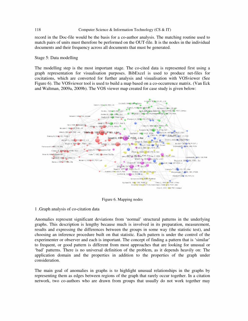
118 Computer Science & Information Technology (CS & IT)
record in the Doc-file would be the basis for a co-author analysis. The matching routine used to
match pairs of units must therefore be performed on the OUT-file. It is the nodes in the individual
documents and their frequency across all documents that must be generated.
Stage 5: Data modelling
The modelling step is the most important stage. The co-cited data is represented first using a
graph representation for visualisation purposes. BibExcel is used to produce net-files for
cocitations, which are converted for further analysis and visualisation with VOSviewer (See
Figure 6). The VOSviewer tool is used to build a map based on a co-occurrence matrix. (Van Eck
and Waltman, 2009a, 2009b). The VOS viewer map created for case study is given below:
Figure 6. Mapping nodes
1 .Graph analysis of co-citation data
Anomalies represent significant deviations from ‘normal’ structural patterns in the underlying
graphs. This description is lengthy because much is involved in its preparation, measurement,
results and expressing the differences between the groups in some way (the statistic test), and
choosing an inference procedure built on that statistic. Each pattern is under the control of the
experimenter or observer and each is important. The concept of finding a pattern that is ‘similar’
to frequent, or good pattern is different from most approaches that are looking for unusual or
‘bad’ patterns. There is no universal definition of the problem, as it depends heavily on: The
application domain and the properties in addition to the properties of the graph under
consideration.
The main goal of anomalies in graphs is to highlight unusual relationships in the graphs by
representing them as edges between regions of the graph that rarely occur together. In a citation
network, two co-authors who are drawn from groups that usually do not work together may
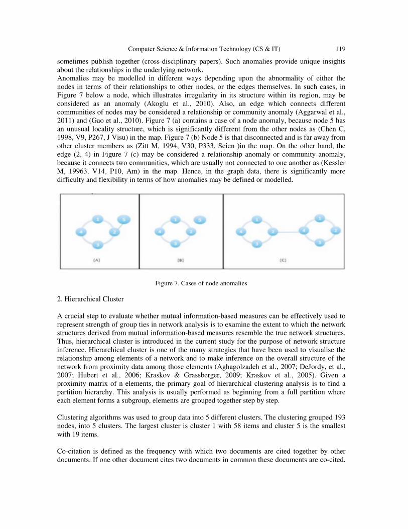
Computer Science & Information Technology (CS & IT) 119
sometimes publish together (cross-disciplinary papers). Such anomalies provide unique insights
about the relationships in the underlying network.
Anomalies may be modelled in different ways depending upon the abnormality of either the
nodes in terms of their relationships to other nodes, or the edges themselves. In such cases, in
Figure 7 below a node, which illustrates irregularity in its structure within its region, may be
considered as an anomaly (Akoglu et al., 2010). Also, an edge which connects different
communities of nodes may be considered a relationship or community anomaly (Aggarwal et al.,
2011) and (Gao et al., 2010). Figure 7 (a) contains a case of a node anomaly, because node 5 has
an unusual locality structure, which is significantly different from the other nodes as (Chen C,
1998, V9, P267, J Visu) in the map. Figure 7 (b) Node 5 is that disconnected and is far away from
other cluster members as (Zitt M, 1994, V30, P333, Scien )in the map. On the other hand, the
edge (2, 4) in Figure 7 (c) may be considered a relationship anomaly or community anomaly,
because it connects two communities, which are usually not connected to one another as (Kessler
M, 19963, V14, P10, Am) in the map. Hence, in the graph data, there is significantly more
difficulty and flexibility in terms of how anomalies may be defined or modelled.
Figure 7. Cases of node anomalies
2. Hierarchical Cluster
A crucial step to evaluate whether mutual information-based measures can be effectively used to
represent strength of group ties in network analysis is to examine the extent to which the network
structures derived from mutual information-based measures resemble the true network structures.
Thus, hierarchical cluster is introduced in the current study for the purpose of network structure
inference. Hierarchical cluster is one of the many strategies that have been used to visualise the
relationship among elements of a network and to make inference on the overall structure of the
network from proximity data among those elements (Aghagolzadeh et al., 2007; DeJordy, et al.,
2007; Hubert et al., 2006; Kraskov & Grassberger, 2009; Kraskov et al., 2005). Given a
proximity matrix of n elements, the primary goal of hierarchical clustering analysis is to find a
partition hierarchy. This analysis is usually performed as beginning from a full partition where
each element forms a subgroup, elements are grouped together step by step.
Clustering algorithms was used to group data into 5 different clusters. The clustering grouped 193
nodes, into 5 clusters. The largest cluster is cluster 1 with 58 items and cluster 5 is the smallest
with 19 items.
Co-citation is defined as the frequency with which two documents are cited together by other
documents. If one other document cites two documents in common these documents are co-cited.

120 Computer Science & Information Technology (CS & IT)
The higher co-citations two documents receive, the more their co-citation strength, and are
semantically related, which can be related to the results from the mapping nodes. Where cluster 1
shows high co-citation frequency indicating higher co-citation strength, cluster 5 has a low co-
citation frequency indicating lower co-citation strength. The relationship strength is based on the
number of citations the two citing documents have in common. After the creation of author co-
citation pairs, the co-citation link strength (Garfield, 1980) is calculated using the following
formula:
Link Strength (AB) = X/(Y-X)
Where X is the number of co-citations of author A and author B, Y is the sum of the total number
of citations of A and the total number of citations of B. This formula normalises the co-citation
link strength by taking into account the total number of citations for both A and B. In item 1
(Small H, 1973) the link strength is 1818 indicating that it is present in cluster 1 and is more co
cited, however item 193 (Farhoomand A, 1987) is shown to have the lowest link strength of 50
and is present in cluster 5 indicating that it less co cited.
3. Visualisation
Analysis of networks has been widely used in a great number of areas to understand relationships
between different entities in a network, as well as behaviour of a network as a whole due to the
interactions between entities within it. Researchers have conducted observations and developed,
experiments on a variety of network analysis techniques including graphical visualisation,
statistical inference and computational algorithms, and built a number of mathematical models in
an effort to understand and predict the behaviour of a network (Newman, 2003). Co-citation data
can be used to study relations among authors or journals; it can be used to construct the maps that
provide a visual representation of the structure of a scientific field. Usually, when using co-
occurrence data, a transformation is applied first to the data. The aim of such a transformation is
to derive similarities from the data. For example, when researchers study relations among authors
based on co-citation data, they typically derive similarities from the data and then analyse these
similarities using hierarchical clustering.
The visualisation helps provide a clear understanding and better representation of the output map
represented at co-citation (see Figure 6). The resulting map visualises a set of objects and the
relations among the objects. Many different types of visualisations can be used. One difference is
between distance-based visualisations and graph-based visualisations. In distance-based
visualisations, the distance between two nodes reflects the relation between the nodes. The
smaller the distance between two nodes, the stronger the relation between the nodes. On the other
hand, in graph-based visualisations in the case study, the distance between two nodes does not
reflect the relation of the nodes. Instead, drawing lines between nodes from the map typically
indicates relations between nodes; the most basic way to visually group nodes is to use colours. If
items have been assigned to clusters, the colour of the circle of an item can be determined by the
cluster in which the item belongs. Item cluster is calculated and translated into colours using a
colour scheme. By default, VOSviewer uses a red-greenblue colour scheme (see Table 1). In the
case study, the relation between nodes is shown by colour and size.
In this colour scheme, red corresponds with the highest item density in cluster 1 and yellow
corresponds with the lowest item density in cluster 5. Furthermore the node size denotes the
number of received citations (White H, 1981, V 32, P163, JAm) being the largest node in the

Computer Science & Information Technology (CS & IT) 121
map, while (Chen C, 2001, V34, P65, Compute) is the smallest node. This can give a great insight
into the relations inside a group and between different groups.
Stage 6: Data evaluation
The main objective of visualising the co-citation data using graphs is to highlight unusual
relationships in the graphs by representing them as edges between regions of the graph that rarely
occur together. In citation network, two co-authors who are drawn from groups that usually do
not work together may sometimes publish together (crossdisciplinary papers). Such anomalies
provide unique insights about the relationships in the underlying network. Hawkins (1980)
defines an anomaly detection based graph as finding “graph objects (nodes/edges) that are rare
and that differ significantly from the majority of in the reference graph nodes.” Graph
investigation technique permits the user to filter out nodes based on visual and semantic
attributes. The method allows filtering-out nodes by their groups (colours). In addition, the
method adopted in this research allows easy modification of filtering options, which may be
dependent on other attributes. Each paper in the collection is associated with the authors who
wrote it and the references it cites. Cluster 5 consists of papers, which covers visualisation of
literature technique. All of the element were based on three types of literature, bibliometrics,
scientometrics, and informetrics. The mutual information for cluster 5 is 0, which confirms that
the elements of that cluster are not linked to other clusters and are considered as collective
anomalies with respect to the entire dataset. Cluster 1 whose mutual information is 93 confirms
that the elements of this cluster share common characteristics/domain area, which are Library and
information science techniques.
In Table where cluster 1 shows high mutual information indicating higher co-citation strength,
cluster 5 has a low mutual information indicating lower co-citation strength.
Table 1. Result of mutual information
We applied mutual information to detect anomalies in the context of co-citation, using the
equation below:
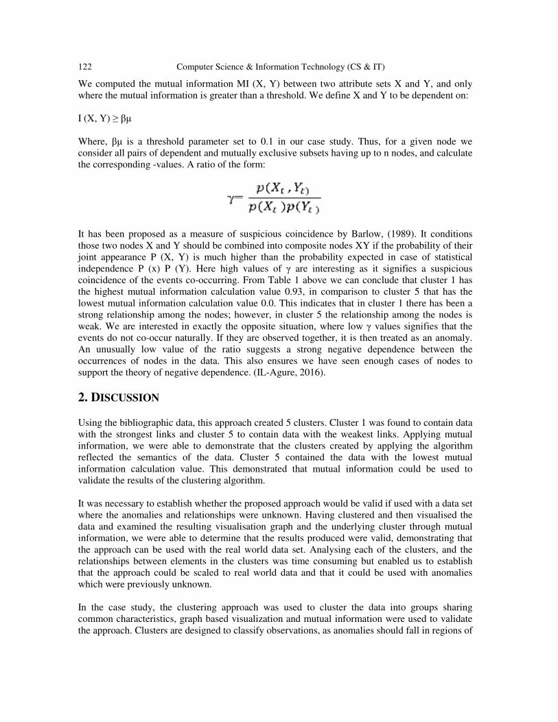
122 Computer Science & Information Technology (CS & IT)
We computed the mutual information MI (X, Y) between two attribute sets X and Y, and only
where the mutual information is greater than a threshold. We define X and Y to be dependent on:
I (X, Y) ≥ βµ
Where, βµ is a threshold parameter set to 0.1 in our case study. Thus, for a given node we
consider all pairs of dependent and mutually exclusive subsets having up to n nodes, and calculate
the corresponding -values. A ratio of the form:
It has been proposed as a measure of suspicious coincidence by Barlow, (1989). It conditions
those two nodes X and Y should be combined into composite nodes XY if the probability of their
joint appearance P (X, Y) is much higher than the probability expected in case of statistical
independence P (x) P (Y). Here high values of γ are interesting as it signifies a suspicious
coincidence of the events co-occurring. From Table 1 above we can conclude that cluster 1 has
the highest mutual information calculation value 0.93, in comparison to cluster 5 that has the
lowest mutual information calculation value 0.0. This indicates that in cluster 1 there has been a
strong relationship among the nodes; however, in cluster 5 the relationship among the nodes is
weak. We are interested in exactly the opposite situation, where low γ values signifies that the
events do not co-occur naturally. If they are observed together, it is then treated as an anomaly.
An unusually low value of the ratio suggests a strong negative dependence between the
occurrences of nodes in the data. This also ensures we have seen enough cases of nodes to
support the theory of negative dependence. (IL-Agure, 2016).
2. DISCUSSION
Using the bibliographic data, this approach created 5 clusters. Cluster 1 was found to contain data
with the strongest links and cluster 5 to contain data with the weakest links. Applying mutual
information, we were able to demonstrate that the clusters created by applying the algorithm
reflected the semantics of the data. Cluster 5 contained the data with the lowest mutual
information calculation value. This demonstrated that mutual information could be used to
validate the results of the clustering algorithm.
It was necessary to establish whether the proposed approach would be valid if used with a data set
where the anomalies and relationships were unknown. Having clustered and then visualised the
data and examined the resulting visualisation graph and the underlying cluster through mutual
information, we were able to determine that the results produced were valid, demonstrating that
the approach can be used with the real world data set. Analysing each of the clusters, and the
relationships between elements in the clusters was time consuming but enabled us to establish
that the approach could be scaled to real world data and that it could be used with anomalies
which were previously unknown.
In the case study, the clustering approach was used to cluster the data into groups sharing
common characteristics, graph based visualization and mutual information were used to validate
the approach. Clusters are designed to classify observations, as anomalies should fall in regions of
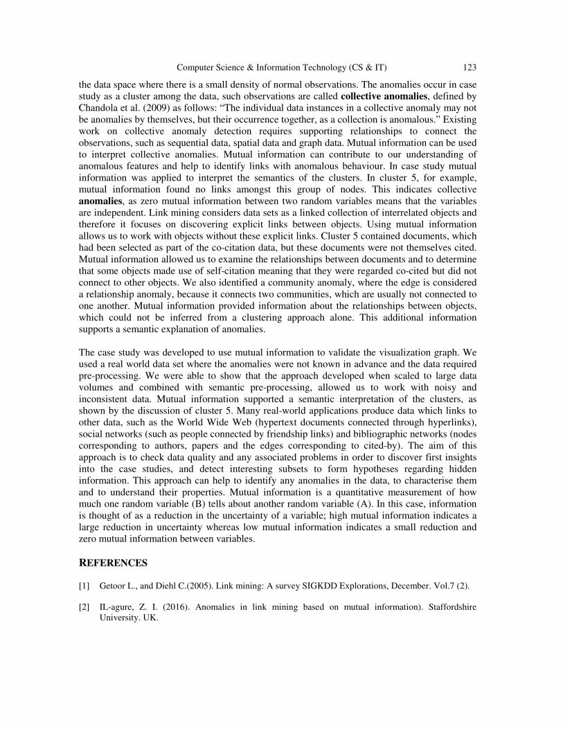
Computer Science & Information Technology (CS & IT) 123
the data space where there is a small density of normal observations. The anomalies occur in case
study as a cluster among the data, such observations are called collective anomalies, defined by
Chandola et al. (2009) as follows: “The individual data instances in a collective anomaly may not
be anomalies by themselves, but their occurrence together, as a collection is anomalous.” Existing
work on collective anomaly detection requires supporting relationships to connect the
observations, such as sequential data, spatial data and graph data. Mutual information can be used
to interpret collective anomalies. Mutual information can contribute to our understanding of
anomalous features and help to identify links with anomalous behaviour. In case study mutual
information was applied to interpret the semantics of the clusters. In cluster 5, for example,
mutual information found no links amongst this group of nodes. This indicates collective
anomalies, as zero mutual information between two random variables means that the variables
are independent. Link mining considers data sets as a linked collection of interrelated objects and
therefore it focuses on discovering explicit links between objects. Using mutual information
allows us to work with objects without these explicit links. Cluster 5 contained documents, which
had been selected as part of the co-citation data, but these documents were not themselves cited.
Mutual information allowed us to examine the relationships between documents and to determine
that some objects made use of self-citation meaning that they were regarded co-cited but did not
connect to other objects. We also identified a community anomaly, where the edge is considered
a relationship anomaly, because it connects two communities, which are usually not connected to
one another. Mutual information provided information about the relationships between objects,
which could not be inferred from a clustering approach alone. This additional information
supports a semantic explanation of anomalies.
The case study was developed to use mutual information to validate the visualization graph. We
used a real world data set where the anomalies were not known in advance and the data required
pre-processing. We were able to show that the approach developed when scaled to large data
volumes and combined with semantic pre-processing, allowed us to work with noisy and
inconsistent data. Mutual information supported a semantic interpretation of the clusters, as
shown by the discussion of cluster 5. Many real-world applications produce data which links to
other data, such as the World Wide Web (hypertext documents connected through hyperlinks),
social networks (such as people connected by friendship links) and bibliographic networks (nodes
corresponding to authors, papers and the edges corresponding to cited-by). The aim of this
approach is to check data quality and any associated problems in order to discover first insights
into the case studies, and detect interesting subsets to form hypotheses regarding hidden
information. This approach can help to identify any anomalies in the data, to characterise them
and to understand their properties. Mutual information is a quantitative measurement of how
much one random variable (B) tells about another random variable (A). In this case, information
is thought of as a reduction in the uncertainty of a variable; high mutual information indicates a
large reduction in uncertainty whereas low mutual information indicates a small reduction and
zero mutual information between variables.
REFERENCES
[1] Getoor L., and Diehl C.(2005). Link mining: A survey SIGKDD Explorations, December. Vol.7 (2).
[2] IL-agure, Z. I. (2016). Anomalies in link mining based on mutual information). Staffordshire
University. UK.

124 Computer Science & Information Technology (CS & IT)
[3] Chandola V., Banerjee A., and Kumar V.(2009) Anomaly Detection. A Survey, ACM Computing
Survey. 41(3). p.15.

124 Computer Science & Information Technology (CS & IT)
INTENTIONAL BLANK

David C. Wyld et al. (Eds) : CCSEIT, AIAP, DMDB, ICBB, CNSA - 2017
pp. 125– 132, 2017. © CS & IT-CSCP 2017 DOI : 10.5121/csit.2017.70612
EVALUATION OF SCALABLE PPRL
SCHEMES WITH A NATIVE LSH
DATABASE ENGINE
Dimitrios Karapiperis
1, Chris T. Panagiotakopoulos
2 and
Vassilios S. Verykios3
1School of Science and Technology, Hellenic Open University, Greece
2Department of Primary Education, University of Patras, Greece
3School of Science and Technology, Hellenic Open University, Greece
ABSTRACT
In this paper, we present recent work which has been accomplished in the newly introduced
research area of privacy preserving record linkage, and then, we present our L-fold redundant
blocking scheme, that relies on the Locality-Sensitive Hashing technique for identifying similar
records. These records have undergone an anonymization transformation using a Bloom filter-
based encoding technique. We perform an experimental evaluation of our state-of-the-art
blocking method against four other rival methods and present the results by using LSHDB, a
newly introduced parallel and distributed database engine.
KEYWORDS
Locality-Sensitive Hashing, Record Linkage, Privacy-Preserving Record Linkage, Entity Resolution
1. INTRODUCTION
A series of economic collapses of bank and insurance companies recently triggered a financial
crisis of unprecedented severity. In order for these institutions to get back on their feet, they had
to engage in merger talks inevitably. One of the tricky points for such mergers is to be able to
estimate the extent to which the customer bases of the constituent institutions are in common, so
that the benefits of the merger can be proactively assessed. The process of comparing the
customer bases and finding out records that refer to the same real world entity, is known as the
Record Linkage, the Entity Resolution or the Data Matching problem.
Record Linkage consists of two main steps. In the first step potentially matched pairs of records
are searched, while in the second step these pairs are matched. The searching step, or commonly
known as blocking, addresses the problem of bringing together for comparison tentative matched
pairs of records, while disregarding the unpromising ones. The searching step should be able to
identify a minimal superset of the matched pairs so that no computational resources are wasted in
comparison operations during the following step. The second step, known as the matching step,
entails the comparison of record pairs which have been brought together for comparison in the
previous step. The matching step is implemented either in an exact or in an approximate manner.
An exact matching of two records can be regarded as a binary decision problem with two possible
outcomes denoting the agreement or disagreement of these records. Approximate matching

126 Computer Science & Information Technology (CS & IT)
comprises the calculation of a continuous value similarity metric that usually assumes values in
the range of [0,1].
When data to be matched is deemed to be sensitive or private, such as health data or data kept by
national security agencies, Privacy-Preserving Record Linkage (PPRL) techniques should be
employed. PPRL investigates how to make linkage computations secure by respecting the privacy
of the data, and imposes certain constraints on the two steps of Record Linkage just described, on
top of the necessary anonymization of the input records. In addition, the anonymization of the
records must be implemented in such a way that (a) no sensitive information in a record is
disclosed to parties other than the owner, (b) the anonymization process to be time and cost
efficient, and (c) the final deliberation about the linking status of a pair of records, that relies on
the comparison of their anonymized form, should be a close approximation of the distance
between their original record counterparts.
In this paper, we elaborate on the details of our proposed flexible L-fold redundant blocking
scheme, which is structured around an efficient technique for searching potentially matching
record pairs. More specifically, our scheme relies on the idea of blocking one record to multiple
groups in order to amplify the probability of inserting similar records into the same block. We use
the so-called Locality-Sensitive Hashing (LSH) technique [1], where we utilize only the necessary
number of hash tables. By doing so, we achieve accurate results without imposing unnecessary
and additional computational overhead. This LSH-based searching method, as shown
experimentally in Section 4, can reduce the number of record pairs that are brought together for
comparison up to 98% of the total comparison space. Experimental results demonstrate the
effectiveness and the superiority of our method by comparing it with four state-of-the-art private
blocking methods.
The structure of the paper is organized as follows: related work is given in Section 2. In Section
3, we illustrate some basic building components used by our approach, while Section 4
formulates the problem being solved. Section 5 exposes the details of our proposed scheme
including a theoretical analysis. Section 6 provides an experimental evaluation of our approach
against four other state-of-the-art blocking methods. Conclusions are discussed in Section 7.
2. RELATED WORK
Several solutions have been proposed in the literature in the field of efficiently blocking(or
searching) similar records. However, the majority of these solutions exhibit poor performance
when applied to large data sets. Next, we provide a categorization of these methods in order to be
able to study their unique characteristics, as well as to be able to compare them.
We divide the blocking solutions into seven main categories:
• The tree-based blocking methods[4,12] use space-partitioning data structures (KD-Trees,
R-Trees etc) to divide a space into non-overlapping regions.
• The hierarchy-based searching which relies on the categorization of records into
generalized hierarchies based on the semantics of values of selected fields [3].
• The reference-based clustering [6,11,13] where global clusters are created based on
publicly available sets of values.
• The multi-sampling reference-based transitive closure clustering [7].

Computer Science & Information Technology (CS & IT) 127
• The neighborhood-based searching [6] which uses the sorted neighborhood method [2]
that creates windows of possibly similar records.
• The randomized hash-based blocking [8, 9, 10] which relies on the Locality-Sensitive
Hashing technique.
3. PROBLEM FORMULATION
Let us assume, two data custodians, Alice and Bob, who wish to link their records. Since, these
data are considered as sensitive, they have to independently anonymize them. These anonymized
records should securely reflect the linking status of the original records, so that the linkage
process can be feasible. The anonymized data sets are then submitted to a Trusted Third Party
(TTP) that will conduct the linkage process.The PPRL process is summarized in Figure 1.
Figure 1. Alice and Bob submit their anonymized data sets to a Trusted Third-Party (TTP), which performs
the linkage task.
Due to the large number of records in modern databases, searching for matching pairs using the
brute-force approach is quite inefficient. Therefore, the TTP should utilize a blocking method that
will mostly generate matching pairs and will provide theoretical guarantees of completeness of
the generated results. PPRL
4. BACKGROUND
4.1 Anonymization of Records Using Bloom Filters
Bloom filters [14] are widely used in the literature due to their effectiveness and simplicity. A
Bloom filter is implemented as a bitmap array of size ρinitialized with zeros. In order to represent
a string as a Bloom filter, we hash each q-gram of that string using a number b of keyed hash
message authentication code (HMAC) functions, such as HMAC-MD5 andHMAC-SHA2 which
associate b positions to certain q-grams (the number of possible q-grams is much larger compared
to the available positions).Guidelines for enhancing the privacy of Bloom filters can be found
in[15]. Figure 2 illustrates the creation of field-level and record-level Bloom filters.
4.2 Hamming Locality Sensitive hashing (HLSH)
This technique guarantees that almost every similar record pair will be identified with high
probability. HLSH works in the binary Hamming metric space S = {0, 1}ρ,where ρdenotes its
dimensionality. Therefore, records should be embedded in S, for example as Bloom filters, in
order to use HLSH. The similarity between a pair of records is defined by a distance threshold θ(d
<= θ).

128 Computer Science & Information Technology (CS & IT)
Figure 2. Creating field-level and record-level Bloom filters.
5. RANDOMIZED LSH-BASED BLOCKING USING HLSH
In this section, we present the details of our LSH-based proposed method and then introduce
LSHDB a freely available similarity database.
5.1 HLSH
HLSH bases its operation on L independent hash tables. Each hash table, denoted by Tl where
l=1,…,L, consists of key-bucket pairs where a bucket hosts a linked list which is aimed at
grouping similar Bloom filter pairs. Each hash table has been assigned a composite hash function
hl which consists of a fixed number k of base hash functions. A base hash function applied to a
Bloom filter returns the value of its j-th position where j ∈ {0,…,ρ-1} chosen uniformly at
random. The result of ahl, which essentially constitutes the blocking key, specifies into which
bucket of some Tl, a Bloom filter will be stored. This randomized process is illustrated in Figure
3.
We assume a pair of Bloom filters of distance d less than or equal to a predefined threshold θas a
similar pair. The smaller the Hamming distance of a Bloom filter pair is, the higher the
probability for ahl to produce the same result. During the matching step, we scan the buckets of
each Tl and formulate Bloom filter pairs.
The optimal number L of the Tl's that should be utilized by HLSH is:
� = ⌈ ���
���� ���⌉,
where p denotes the probability of a base hash function of producing the same result by hashing
two similar Bloom filters. By using this structure, each similar Bloom filter pair will be returned
with high probability 1 -δ, as δ is usually set to a small value, say δ=0.1.

Computer Science & Information Technology (CS & IT) 129
Figure 3. Hashing a pair of similar Bloom filters using HLSH.
5.2 THE LSHDB PARALLEL AND DISTRIBUTED ENGINE
LSHDB[16] is the first parallel and distributed engine for record linkage and similarity search.
LSHDB materializes an abstraction layer to hide the mechanics of the Locality-Sensitive
Hashing, which is used as the underlying similarity search engine. LSHDB creates the appropriate
data structures from the input data and persists these structures on disk using a noSQL engine. It
inherently supports the parallel processing of distributed queries, is highly extensible, and is easy
to use.
Upon the creation of a database, termed as data store, the developer needs to specify only two
parameters: (i) the LSH method that will be employed, e.g.,Hamming, Min-Hash, or Euclidean
LSH, and (ii) the underlying noSQL data engine that will be used to host the data. After these
decisions have been made, LSHDB builds the necessary hash tables, which are stored on disk by
the chosen noSQL system. To the best of our knowledge, LSHDB is the first record linkage and
similarity search system in which parallel execution of queries across distributed data stores is
inherently crafted to achieve fast response times.
6. EXPERIMENTAL EVALUAION
We evaluate HLSH in terms of (a) the accuracy in finding the truly matching record pairs, (b) the
efficiency in reducing the number of candidate pairs, and (c) the execution time. We use two
semi-synthetic data sets, denoted by A and B, of size equal to 1,000,000 records each, extracted
from the NCVR list (http://dl.ncsbe.gov/index.html?prefix=data/). Insert, edit, delete, and

130 Computer Science & Information Technology (CS & IT)
transpose operations, chosen in random order, are used to perturb the values of each field of
certain marked records from A, which are placed in set B. For the experiments, we used a simple
PC with an Intel i5-2400 and 16 GB RAM. The software components were developed using the
Java programming language (JDK 1.8).
The Pairs Completeness(PC) and the Reduction Ratio (RR) metrics are employed to evaluate the
accuracy in identifying the matching record pairs and the reduction of the comparison space,
respectively. PC denotes the number of the truly matching record pairs identified by each method.
Conversely, RR indicates the percentage of the reduction of the total comparison space between
the two data sets. Specifically, the fraction of the number of distance computations performed to
the total number of all possible distance computations subtracted from 1. We ran each experiment
10 times, and plotted the average values in the figures shown below.
We compared HLSH with four state-of-the-art blocking methods. The first of these methods,
denoted by KDT [12], relies on kd-trees to formulate blocks of records which have previously
been embedded into the Euclidean space. The second method, symbolized by HG [3], categorizes
the records into generalized hierarchies based on the semantics of values of selected attributes.
PHN [5] uses phonetic encoding functions to generalize strings, while AHC [11] employs
agglomerative hierarchical clustering to create blocks, which are generated by the TTP for a set of
public reference values of a chosen field. Then, each data custodian assigns her records into the
formulated blocks.
Figure 4.The Pairs Completeness rates.
Figure 4 illustrates the PC rates achieved by each method. We observe that HLSH and AHC
achieve the highest scores. However, we have to note that the performance of AHC is highly
dependent on the choice of the reference values. We tested several sets of reference values but
only achieved high PC rates, when those sets were supersets of the field values. Conversely, if
those sets were not supersets of the field values, the PC rates dropped considerably below 70%.
HG and PHN achieved stable performance, whose rates, however, were also around 70%. KDT
exhibited large deviations from its mean rate, mainly due to the deficiencies of the embedding
method used.
The reduction of the comparison space, as measured by the RR, is shown in Figure 5. HLSH and
AHC exhibit comparable performance reaching almost 98% reduction. PHN scores rates very
close to 90%, while HG and KDT exhibit inferior performances.

Computer Science & Information Technology (CS & IT) 131
7. CONCLUSIONS
Linking large collections of records by simultaneously protecting their privacy has arisen recently
as an intriguing problem in the core of the domain known as Privacy-Preserving Record Linkage.
In this paper, we expose the details of HLSH blocking method, and experimentally compare it
with four state-of the-art private blocking methods in the context of LSHDB, an newly introduced
data engine for big data computations. HLSH outperformed these methods in terms of the
accuracy of the results as well as the running time.
Figure 5.The Reduction Ratio.
REFERENCES
[1] A.Gionis, P. Indyk, and R. Motwani. Similarity search in high dimensions via hashing. In VLDB,
pages 518–529, 1999.
[2] M.A. Hernandez and S.J. Stolfo. Real world data is dirty: Data cleansing and the merge/purge
problem. Data Min. And Knowl.Disc., 2(1):9 – 37, 1988.
[3] A. Inan, M. Kantarcioglou, E. Bertino, and M. Scannapieco. A hybrid approach to private record
linkage. In ICDE, pages 496 – 505, 2008.
[4] A. Inan, M. Kantarcioglu, G. Ghinita, and E. Bertino. Private record matching using differential
privacy. In EDBT, pages 123 – 134, 2010.
[5] A. Karakasidis and V.S. Verykios. Privacy preserving record link a geusing phonetic codes. In BCI,
pages 101 – 106, 2009.
[6] A. Karakasidis and V.S. Verykios. A Sorted Neighborhood Approach to multidimensional Privacy
Preserving Blocking. In ICDMWorkshops, pages 937 – 944, 2012.
[7] A. Karakasidis, G. Koloniari, and V. S. Verykios. Scalable Blocking for Privacy Preserving Record
Linkage. In KDD, pages 101 – 106, 2015.
[8] D. Karapiperis and V.S. Verykios. An LSH-based Blocking Approach with a Homomorphic Matching
Technique for Privacy-PreservingRecord Linkage. TKDE, 27(4):909–921, 2015.
[9] D. Karapiperis and V.S. Verykios. A fast and efficient HammingLSH-based scheme for accurate
linkage. KAIS, pages 1–24, 2016.

132 Computer Science & Information Technology (CS & IT)
[10] H. Kim and D. Lee. Fast Iterative Hashed Record Linkage for Large-Scale Data Collections. In
EDBT, pages 525 – 536, 2010.
[11] M. Kuzu, M. Kantarcioglu, A. Inan, E. Bertino, E. Durham, and B. Malin. Efficient privacy-aware
record integration. In EDBT,pages 167 – 178, 2013.
[12] M. Scannapieco, I. Figotin, E. Bertino, and A.K. Elmagarmid. Privacy preserving schema and data
matching. In SIGMOD, pages 653 – 664,2007.
[13] D. Vatsalan, P. Christen, and V. Verykios. Efficient two-party private blocking based on sorted
nearest neighborhood clustering. In CIKM,pages 1949 – 1958, 2013.
[14] R. Schnell, T. Bachteler, and J. Reiher. Privacy-preserving record linkage using Bloom filters. Central
Medical Inf. and Decision Making, 9, 2009.
[15] F. Niedermeyer, S. Steinmetzer, Martin M. Kroll, and R. Schnell.Cryptanalysis of Basic Bloom
Filters Used for Privacy Preserving Record Linkage. JPC, 6(2), 2014.
[16] D. Karapiperis, A. Gkoulalas-Divanis, and V. Verykios. LSHDB: a parallel and distributed engine for
record linkage and similarity search. In ICDMW (DEMO), pages 1-4, 2016.
AUTHORS
Dr.DimitriosKarapiperis is a post-doctoral associate with the Hellenic Open
University (HOU), Greece. He holds a PhD degree from HOU, an MSc degree from
the University of York, UK, and a BSc degree from the Technological Institute of
Thessaloniki, Greece. His research interests lie in the areas of privacy-preserving
record linkage, entity resolution, and similarity search, where he develops
randomized algorithms and data structures.
Chris T. Panagiotakopoulos is α Professor with the Division of General Sciences,
Department of Primary Education at the University of Patras, Greece. His research
interest is focused on the Educational Technology and especially on the development
and use of educational software, educational robotics, web technologies and open and
distance learning.
Vassilios S. Verykios received the Diploma degree in Computer Engineering from
the University of Patras, Greece in 1992, and the MSc and the PhD degrees from
Purdue University, USA in 1997 and 1999, respectively. Since January of 2016, he is
a Professor in the School of Science and Technology at the Hellenic Open University
in Greece where he has been the Director of the Graduate Program on Information
Systems since 2012.

David C. Wyld et al. (Eds) : CCSEIT, AIAP, DMDB, ICBB, CNSA - 2017
pp. 133– 143, 2017. © CS & IT-CSCP 2017 DOI : 10.5121/csit.2017.70613
THERMAL IMAGING USING CNN AND
KNN CLASSIFIERS WITH FWT, PCA AND
LDA ALGORITHMS
Chigozie Orji , Evan Hurwitz and Ali Hasan
Department of Electrical and Electronic Engineering Science,
University of Johannesburg, Johannesburg, South Africa
ABSTRACT
This paper deals with the problem of errors in a biometric system that may arise from poor
lighting and spoofing. To tackle this, images from the Terravic Facial Infrared Database have
been used with Fast Wavelet Transform (FWT), an ensemble of classifiers and feature
extractors, to reduce errors encountered in thermal facial recognition. By dividing the image set
into a training set, comprising 1000 thermal images of 10 persons wearing glasses (X) and a
test set comprising 100 image samples (y), of the same persons in glasses. A mean percentage
error of 0.84% was achieved, when a Convolutional Neural Network (CNN) was used to classify
the image set (y), after training with (X). However, when the images where pre-processed with
Principal Component Analysis (PCA), Linear Discriminant Analysis (LDA) and k-Nearest
Neighbors (KNN) classifier, a mean percentage error of 0.68% was achieved with the CNN
classifier.
KEYWORDS
Thermal imaging, ensemble of classifiers, Deep Convolutional Neural Networks, K-Nearest
Neighbors, Eigen Vectors, Principal Component Analysis, Linear Discriminant Analysis,
biometrics, sensing, imaging, security
1. INTRODUCTION
The use of physical and behavioural attributes to recognize people is known as "biometric
authentication" and this involves recognizing persons using attributes such as iris, finger print,
voice sample, gait or facial features [1]. Among these attributes, the face possesses a unique set of
features, for automatic detection and authentication of a person through computer vision. To
successfully achieve this, under varying weather and lighting conditions, thermal imaging can be
utilized to deal with some of the challenges associated with standard imaging methods. However,
certain issues still exist with thermal images, such as the low quality of the images and the
inability of humans to easily recognize persons in thermal images [2]. As a result feature
extraction based on a robust approach, is required for person recognition using thermal images to
reduce errors. In this paper, a comprehensive experimental study on facial recognition in thermal
images is presented; FWT [3], PCA [4] and LDA [5] have been applied for facial feature
Extraction and KNN [6] with CNN algorithms for human classification [7].

134 Computer Science & Information Technology (CS & IT)
The focus here is to exploit the combined strengths of FWT, PCA, popularly known as Eigen
faces and LDA, popularly known as Fisher faces [8]. To improve feature detection from 1000
facial thermal images, in the Terravic Facial Infrared Database [9] and achieve improved
classification of the features, using KNN and CNN classifiers. Experiments show that the mean
squared error for the CNN classifier is reduced through pre-processing and pre-classification with
PCA, LDA and KNN algorithms respectively.
2. RELATED WORK Debotosh et al. [10] experimented using the Terravic Facial IR Database, with two methods for
face recognition: (1) Haar wavelet transform and (2) Local Binary Pattern (LBP). (1) The Haar
wavelet transform method was applied with a cropping technique by binarizing the thermal faces,
to separate them from their background, before feature extraction with Haar wavelet transform.
(2) For the LBP method, each facial image was converted into 161 sub images, each comprising 8
by 8 pixels. These were concatenated into rows; which were processed to yield a more refined set
of features using PCA. The reduced images, where then classified using a multi layer feed
forward neural network and a minimum distance classifier. The weakness of this method is that,
through cropping of the faces, some soft biometric information (physical and behavioural, such as
material accessories worn) which can be used, to improve the matching accuracy of the
classification system, are lost [11],[12],[13],[14]. Brais et al. propose recognition, in thermal
images, through the detection of the eyes, nostrils and mouth, the subsequent decomposition into
a feature vector with Haar wavelets, then classification using SVM and Gentle boost [15].
Christian et al. achieved an error rate reduction of up to 80% on LWIR images, on the AMROS
and OTCBVS benchmark datasets, with detection using Maximally Stable Extremal Regions
(MSER) and classification with a Convolutional Neural Network (CNN). With MSER acting as a
hot spot detector and CNN as a classifier for detected hot spots [16].
The ensembling of classifiers, help algorithms achieve better results, however this has to be done
with an understanding of the needed computing power and a knowledge of the strengths and
weaknesses of individual classifiers [17], [18]. For deep CNN, Alex et al. [19] used non-
saturating neurons and a GPU implementation of the CNN, to classify 1.2 million high resolution
images. Despite their ability to learn complex patterns, CNNs are known to be easily fooled [20],
[21]. Research work has been done, in the area of understanding CNNs, their flaws and ways to
make them work better [22], [23], [24]. One is by using them with a less complex classifier, such
as least squares regression and a linear classifier, this combination was used to achieve high
training speed with low implementation complexity, on the MNIST test set, NORB-small and
SVHN databases [25]. The same approach was used to improve the CNN algorithm’s efficiency
and reduce errors by [26]. Other variations of CNN-based classification are possible and would
require additional research to discover. In an attempt to do this, we have analyzed the merits of
ensembling a local learning algorithm, such as K-Nearest Neighbours (KNN) with Convolutional
Neural Networks (CNN).
3. THE PROPOSED METHOD
We propose a combination-based approach for classifiers on the Terravic Infrared Database. By
experimenting with a wavelet transform technique and known feature extraction algorithms. We
found out that the combination of a spot classifier algorithm (KNN) and a deep learning classifier

Computer Science & Information Technology (CS & IT) 135
algorithm (CNN) reduces errors, when attempting to make predictions on samples not in the
training set.
Figure 1. Proposed structure for CNN thermal face recognition combined with KNN.
3.1. The Terravic Infrared Database
The Terravic Facial Infrared Database is a sub set of the OTCBVS benchmark data set, a public
database available, exclusively for educational and research purposes, for experiments in the area of computer vision algorithms and for exploring the advantages that derivable from using the
invisible spectrum in real world applications. The benchmark comprises 12 separate categories of thermal images of which the Terravic Facial IR Databases is one [9].
Figure 2. Sample images from a glasses wearing group in the Terravic Facial Infrared Database

136 Computer Science & Information Technology (CS & IT)
3.2. Fast Wavelet Transform (FWT)
Wavelet transform techniques are commonly used in image processing applications involving
images with low signal-to-noise ratio such as thermal images [27].
It works by dividing an image into high and low frequency areas that can be represented
graphically as sub bands. Several wavelet transform methods exist such as the Discrete Wavelet
Transform (DWT) and Fast Wavelet Transform [3]. The Fast Wavelet Transform method, is used
here, among the transform tools in Large Time Frequency Analysis Toolbox (LTFAT), in Octave,
because of its simplicity and its application to thermal imaging [28].
Figure 3. Visualized FWT of glass wearing images, from the Terravic Facial Infrared Database, showing
spatial and frequency data represented using 4 sub bands
3.3. Principal Component Analysis (PCA)
PCA is a transform technique used for extracting points of highest variance or principal
components, from data through an orthogonal projection of these points onto a new coordinate in
a lower dimensional feature space. For on the spot classification using algorithms such as KNN,
the fewer the number of components the easier it is to compute the most proximal example in the
feature space [29]. Mathematically this is represented as:
AV = λV (1)
Where A=Matrix,V = Eigen vector matrix, λ = Diagonal matrix of corresponding Eigen values
The figure below shows Eigen faces from the thermal facial dataset, after principal component analysis.

Computer Science & Information Technology (CS & IT) 137
Figure 4. A Eigen face feature set, visualized after Principal Component Analysis (PCA), from the Terravic
Facial Infrared Database, glass wearing images.
3.4. Linear Discriminant Analysis (LDA)
Fisher face is an enhancement of the Eigen face technique, achieving dimensionality reduction
using Linear Discriminant Analysis (LDA). Unlike PCA, it seeks a projection axes between
images, upon which to measure the variance of their data points, by maximizing between class
differences and minimizing within class differences [30]. Mathematically this is represented as:
SbV = λ SwV (2)
Where Sw = within class differences, Sb = between class differences, V = The eigen vector
matrix, λ = Eigen values
The figure below shows Fisher faces from the thermal facial dataset, after Linear Discriminant
analysis.
Figure 5. A Fisher face feature set, visualized after Linear Discriminant Analysis (LDA), from the Terravic
Facial Infrared Database, glass wearing images.

138 Computer Science & Information Technology (CS & IT)
3.5. K-Nearest Neighbors
For these experiments, involving PCA, LDA and K-Nearest Neighbours (KNN), we have used
the Byte fish face recognition tool box [31]. KNN is an instance based learning classifier, which
works without parameters but with the K closest training examples, in the feature space, as its
input. Given a training set ranging from M1 to MK, it finds the best k means sample that can be
used to represent the entire training set and classifies successive points Ni, based on their
proximity P to the means.
C (Ni) = P (Ni, Mk) (3)
Figure 6. KNN local classification method based on distance from training example
3.6. Convolutional Neural Network (CNN)
We have used CNN tools from, Rasmus Berg Palm's, deep learning tool box [33]. The structure
of our deep neural network, consists of 6 layers an input layer, 2 convolution layers, with 2 sub
sampling layers and an output layer, this is shown in table I below. We trained the model several
times with different initial seeds for each training session, the CNN network did a 100 epochs
running 50 batches per epoch. After which the mean-squared error for the batch was plotted
against the number of iterations. An error of 0.86% was achieved at the 100th iteration of the
gradient descent.
Table 1. Convolusional Network Architecture
Activation function Sigmoid
Input Layer 1
Number Convolusion Layers (CL) 2
Convolusion layer Output maps 6
Convolusion layer Kernel size 5
Number Sub sampling (pooling) layers 2
Sub sampling layers scale 2
Alpha 1
Batch size 50
Number of epochs 100

Computer Science & Information Technology (CS & IT) 139
Figure 7. CNN deep classification method based on convolution and sub sampling
4. EXPERIMENTS
4.1. Fast Wavelet Transform We experimented with Fast Wavelet Transform, using the Large Time-Frequency Analysis
Toolbox (LTFAT) in Octave and produced 4 sub-bands from the 76800 by 144 data matrix,
shown in Fig.3. The fourth sub band being the richest in time-frequency (TF) features was used to
develop a confidence matrix (38400 by 144) which was subjected to Principal Component and
Linear Discriminant Analysis.
4.2. Feature Extraction
Both PCA and LDA performed similarly on the TF features, when used with KNN for
classification, producing a test set accuracy up to 16.67%, for 20 PCA and LDA components.
4.3. Classification
After training and classification with CNN and then re-training and classifying with KNN, PCA
and LDA, it was observed that KNN’s local prediction method improved CNN’s deep and
exhaustive approach to classification, and reduced errors on the TF feature set. Figures 6 and 7
below show this improvement.
Figure. 8. CNN classification without PCA, LDA and KNN, using the time-frequency (TF) features, of
images from the Terravic Facial Infrared Database, glass wearing images.

140 Computer Science & Information Technology (CS & IT)
Figure. 9. CNN classification with PCA, LDA and KNN , using the time-frequency(TF) features, of images
from the Terravic Facial Infrared Database, glass wearing images.
4.4. Classification Explained
The combination of FWT and CNN algorithm, achieves an average of 0.84% error, on the test set
after training, by also recognizing 9 people out of 10 among 100. While the combination of FWT,
PCA, LDA and KNN algorithms after training, achieves 0.86% error on the test set, by
recognizing 9 people out of 10 among 100. The combined predictions show each algorithm
making up for the shortcoming of the other, as the 1 person not recognized by the CNN classifier,
was recognized by KNN and vice versa; making the union of results from both classifiers, yield a
total decrease in the percentage error.
4.5. Results Analysis
Comparing the CNN and KNN algorithm approaches to classifying thermal facial images, we
find that (1) Fast Wavelet Transform helped PCA and LDA with time-frequency (TF) features,
for analysis on the facial thermal images. (2) KNN with PCA and LDA generalize well to new
examples for a smaller test set of similar images, such as 40 images of 2 – 5 people wearing
glasses, but do not for a larger test set, of up to 100 images of the same people. (3) CNN
generalizes well for a large test set but doesn’t do so for a smaller one comprising images of the
same people. (4) The use of CNN with KNN, PCA and LDA on a large test set, improves
classification, among images for both those with close distance in similarity, using soft biometric
features such as glass wearing, and those without it.
5. CONCLUSION
The K-Nearest Neighbours (KNN) simplicity, based on distance geometrically, is demonstrated
using the Terravic Facial Infrared Database. It moderates decisions made by the Convolutional
Neural Networks (CNN), when classifying thermal facial images that are similar, in terms of soft-
biometric features. Other soft biometric features should be experimented with, using CNN, FWT
and KNN, and the results compared with the research we have presented in this paper.

Computer Science & Information Technology (CS & IT) 141
Table 2. Experimental Results
Feature Extraction FWT Result
FWT Sub-band 1 9600 features
FWT Sub-band 2 9600 features
FWT Sub-band 3 19200 features
FWT Sub-band 4 38400 features
Algorithm Result
FWT Sub-band 4 +20 PCA+KNN TPR 8.33%
FWT Sub-band 4 +20 PCA+KNN Accuracy 16.67%
FWT Sub-band 4 +20 LDA+KNN TPR 8.33%
FWT Sub-band 4 +20 LDA+KNN Accuracy 16.67%
FWT Sub-band 4 +20PCA+120 LDA+KNN 0.86% Error (Training set)
FWT Sub-band 4 +20PCA+120 LDA+KNN 0.89% Error (Test set)
FWT Sub-band 4 +20PCA+120 LDA+KNN 0.89% Error (CV set)
FWT Sub-band 4 + CNN (session 1) 0.842% Error (Training, test and CV sets)
FWT Sub-band 4 + CNN (session 2) 0.845% Error (Training, test and CV sets)
FWT Sub-band 4 + CNN (session 3) 0.848% Error (Training, test and CV sets )
FWT Sub-band 4 + CNN 0.84% Error (Average)
FWT Sub-band 4 + CNN + FWT Sub-band 4
+20PCA+120 LDA+KNN
0.68% Error
ACKNOWLEDGEMENTS
The financial assistance of the National Research Foundation (NRF) towards this research is
hereby acknowledged. Opinions expressed and conclusions arrived at, are those of the author and
are not necessarily to be attributed to the NRF.
REFERENCES [1] A. K. Jain, P. J. Flynn, and A. Ross. Handbook of Biometrics. Springer, 2007.
[2] G. Bebis, A. Gyaourova, S. Singh, and I. Pavlidis, "Face Recognition by Fusing Thermal Infrared and
Visible Imagery", Image and Vision Computing, vol. 24, no. 7, pp. 727-742, 2006.
[3] G. Beylkin, R. Coifman, and V. Rokhlin. Fast wavelet transforms and numerical algorithms I.
Communications on Pure and Applied Mathematics, 44(2):141–183, March 1991.
[4] M. Turk and A. Pentland, “Face Recognition Using Eigenfaces,” Proc. IEEE Conf. on Computer
Vision and Pattern Recognition, 1991, pp. 586-591.
[5] P.N. Belhumeur, J.P. Hespanha and D.J.Kriegman, “Eigenfaces vs. Fisherfaces: Recognition using
class specific linear projection” IEEE Trans. Pattern Analysis and Machine Intelligence, vol. 19, no.
7, pp. 711-720, Jul. 1997.
[6] A. Coates and A. Y. Ng, “Learning feature representations with k-means,” in Neural Networks:
Tricks of the Trade. Springer, 2012, pp. 561–580.
[7] X. Chen, P. Flynn, and K. Bowyer, “PCA-based face recognition in infrared imagery : Baseline and
comparative studies,” IEEE International Workshop on Analysis and Modeling of Faces and
Gestures, pp. 127–134, October 2003. Vision and Modeling Group, The Media Laboratory

142 Computer Science & Information Technology (CS & IT)
[8] Lu, J., Plataniotis, K., Venetsanopoulos, A.: Face recognition using LDA-based algorithms. IEEE
Transactions on Neural Networks 14 (2003) 195–200.
[9] IEEE OTCBVS WS Series Bench; Roland Miezianko, Terravic Research Infrared Database.
[10] D. Bhattacharjee, A. Seal, S. Ganguly, M. Nasipuri, and D.K. Basu, “A Comparative Study of Human
Thermal Face Recognition Based on Haar Wavelet Transform and Local Binary Pattern,”
Computational Intelligence and Neuroscience, vol. 2012, Article ID 261089, 12 pages, 2012.
oi:10.1155/2012/261089.
[11] D. Reid and M. Nixon. Using comparative human descriptions for soft biometrics. In Proc. of
International Joint Conference on Biometrics, 2011.
[12] A. Dantcheva, C. Velardo, A. D’Angelo, and J.-L. Dugelay. Bag of soft biometrics for person
identification. New trends and challenges. Multimedia Tools and Applications, 51:739–777, 2011.
[13] A.K. Jain, S.C. Dass, and K. Nandakumar. Soft biometric traits for personal recognition systems. In
Proceedings of ICBA, pages 1–40. Springer, 2004.
[14] A.K. Jain, S. C. Dass, and K. Nandakumar. Can soft biometric traits assist user recognition? In
Proceedings of SPIE, volume 5404, pages 561–572, 2004
[15] B. Martinez, X. Binefa, and M. Pantic. Facial component detection in thermal imagery. In Proc. IEEE
Conference on Computer Vision and Pattern Recognition Workshops, pages 48–54, 2010.
[16] C. Herrmann, T. Müller, D. Willersinn, J. Beyerer, "Real-time person detection in low-resolution
thermal infrared imagery with MSER and CNNs", in Proc. Electro-Optical and Infrared Systems,
SPIE, 2016.
[17] T. G. Dietterich, “Ensemble methods in machine learning,” International workshop on multiple
Classifier systems, p. Springer.
[18] A. Rahman and S. Tasnim, “Ensemble Classifiers and Their Applications: A Review,” International
Journal of Computer Trends and Technology (IJCTT), vol. 10, no. 1, 2014.
[19] A. Krizhevsky, I. Sutskever and G. Hinton . ImageNet Classification with Deep Convolutional Neural
Networks. In Advances in Neural information Processing Systems 25, pages 1106-1114, 2012.
[20] Nguyen A, Yosinski J, Clune J. Deep Neural Networks Are Easily Fooled: High Confidence
Predictions for Unrecognizable Images. CVPR. 2015; 427-436.
[21] Szegedy C et al. Intriguing properties of neural networks. CoRR. 2013.
[22] Szegedy C et al. Going Deeper with Convolutions. CoRR. 2014.
[23] Oquab M et al. Learning and transferring mid-level image representations using convolutional neural
networks. CVPR. 2014; 1717-1724.
[24] Szegedy C et al. Rethinking the Inception Architecture for Computer Vision. arXiv preprint. 2015.
[25] McDonnell MD, Vladusich T. Enhanced image classification with a fast-learning shallow
convolutional neural network. In Proceedings of International joint conference on neural networks
(IJCNN'2015), Killarney, Ireland, 12-17 July 2015.

Computer Science & Information Technology (CS & IT) 143
[26] G.-B. Huang, Z. Bai, L. L. C. Kasun, and C. M. Vong, "Local receptive fields based extreme learning
machine, " IEEE Computational Intelligence Magazine, vol. 10, pp. 18-29, 2015.
[27] P.L. Søndergaard, B. Torrésani, P.Balazs. The Linear Time-Frequency Analysis Toolbox.
International Journal of Wavelets, Multiresolution Analysis and Information Processing, 10(4), 2012.
[28] L. Sirovitch and M. Kirby, “Low-Dimensional Procedure for the Characterization of Human Faces,”
J. Optical Soc. of Am. A, vol. 2, pp. 519-524, 1987.
[29] M. Turk and A. Pentland, “Eigenfaces for Recognition,” J. Cognitive Neuroscience, vol. 3, no. 1,
1991.
[30] R.A. Fisher, “The Use of Multiple Measures in Taxonomic Problems,” Ann. Eugenics, vol. 7, pp.
179-188, 1936.
[31] P. Wagner, "Bytefish face recognition algorithms for MATLAB/GNU Octave and Python," 2015.
[Online]. Available: https://github.com/bytefish/facerec
[32] L. Bottou and V. Vapnik. “Local learning algorithms,” Neural Computation, 4(6), pp. 888-901, 1992.
[33] "R. B. Palm,"Prediction as a candidate for learning deep hierarchical models of data," 2012. [Online].
Available: http://www2.imm.dtu.dk/pubdb/views/publication_details.php?id=6284

AUTHOR INDEX
Ali Hasan 133
Andrew Roberts 01
Assane Wade 75
Belsam Attallah 113
Bernard V 101
Bjoern Flemming Broberg 01
Chigozie Orji 133
Chris T. Panagiotakopoulos 125
Cousin P-Y 101
Dimitrios Karapiperis 125
Enrique Carlos Segura 27
Eric Nyiri 35
Erion Çano 15
Evan Hurwitz 133
Farah Dhib Tatar 85
Francis Grady 01
Geir Gil Martens 01
Giovanna Di MarzoSerugendo 75
Gustavo Lado 27
Joris Guerin 35
Junfei Qiao 53
Kjetil Vatland Johansen 01
Lefaillet A 101
Marius Rafailescu 09
Maurizio Morisio 15
Mugaruka M 101
Olivier Gibaru 35
Olugbenga Adejo 67
Pieyre Le Loher 01
Qiang Fu 01
Qili Chen 53
Raibaud C 101
Stephane Thiery 35
Thomas Connolly 67
Vassilios S. Verykios 125
Yi Ming Zou 53
Zakea Il-agure 113