Embed Size (px)
Citation preview

Computer Science & Information Technology 132


David C. Wyld,
Dhinaharan Nagamalai (Eds) Computer Science & Information Technology
4th International Conference on Computer Science and
Information Technology (COMIT 2020),
November 28~29, 2020, Dubai, UAE
AIRCC Publishing Corporation

Volume Editors
David C. Wyld,
Southeastern Louisiana University, USA
E-mail: [email protected]
Dhinaharan Nagamalai,
Wireilla Net Solutions, Australia
E-mail: [email protected]
ISSN: 2231 - 5403 ISBN: 978-1-925953-30-5
DOI: 10.5121/csit.2020.101601- 10.5121/csit.2020.1011610
This work is subject to copyright. All rights are reserved, whether whole or part of the material is
concerned, specifically the rights of translation, reprinting, re-use of illustrations, recitation,
broadcasting, reproduction on microfilms or in any other way, and storage in data banks.
Duplication of this publication or parts thereof is permitted only under the provisions of the
International Copyright Law and permission for use must always be obtained from Academy &
Industry Research Collaboration Center. Violations are liable to prosecution under the
International Copyright Law.
Typesetting: Camera-ready by author, data conversion by NnN Net Solutions Private Ltd.,
Chennai, India

Preface
The 4th International Conference on Computer Science and Information Technology (COMIT
2020),November 28~29, 2020, Dubai, UAE, 4th International Conference on Signal, Image
Processing (SIPO 2020), 4th International Conference on Artificial Intelligence, Soft Computing
and Applications (AISCA 2020), International Conference on Machine Learning, IOT and
Blockchain (MLIOB 2020) and International Conference on Big Data & Health Informatics
(BDHI 2020) was collocated with 4th International Conference on Computer Science and
Information Technology (COMIT 2020). The conferences attracted many local and international
delegates, presenting a balanced mixture of intellect from the East and from the West.
The goal of this conference series is to bring together researchers and practitioners from
academia and industry to focus on understanding computer science and information technology
and to establish new collaborations in these areas. Authors are invited to contribute to the
conference by submitting articles that illustrate research results, projects, survey work and
industrial experiences describing significant advances in all areas of computer science and
information technology.
The COMIT 2020, SIPO 2020, AISCA 2020, MLIOB 2020 and BDHI 2020 Committees
rigorously invited submissions for many months from researchers, scientists, engineers, students
and practitioners related to the relevant themes and tracks of the workshop. This effort guaranteed
submissions from an unparalleled number of internationally recognized top-level researchers. All
the submissions underwent a strenuous peer review process which comprised expert reviewers.
These reviewers were selected from a talented pool of Technical Committee members and
external reviewers on the basis of their expertise. The papers were then reviewed based on their
contributions, technical content, originality and clarity. The entire process, which includes the
submission, review and acceptance processes, was done electronically.
In closing, COMIT 2020, SIPO 2020, AISCA 2020, MLIOB 2020 and BDHI 2020 brought
together researchers, scientists, engineers, students and practitioners to exchange and share their
experiences, new ideas and research results in all aspects of the main workshop themes and
tracks, and to discuss the practical challenges encountered and the solutions adopted. The book is
organized as a collection of papers from the COMIT 2020, SIPO 2020, AISCA 2020, MLIOB
2020 and BDHI 2020.
We would like to thank the General and Program Chairs, organization staff, the members of the
Technical Program Committees and external reviewers for their excellent and tireless work. We
sincerely wish that all attendees benefited scientifically from the conference and wish them every
success in their research. It is the humble wish of the conference organizers that the professional
dialogue among the researchers, scientists, engineers, students and educators continues beyond
the event and that the friendships and collaborations forged will linger and prosper for many
years to come.
David C. Wyld,
Dhinaharan Nagamalai (Eds)

General Chair Organization David C. Wyld, Southeastern Louisiana University, USA
Dhinaharan Nagamalai, Wireilla Net Solutions, Australia
Program Committee Members
Abdelaziz Mamouni, Faculty of Sciences Ben M’sik,Morocco
Abdolreza hatamlou, Islamic Azad University, Iran
Abdulhamit Subasi, Effat University, Saudi Arabia
Abdullah, Adigrat University,Africa
Abel Gomes, University of Beira Interior, Portugal
Abel J.P. Gomes, Univ. Beira Interior, Portugal
Addisson Salazar, Polytechnic University of Valencia, Spain
Adrian Olaru, University Politehnica of Bucharest, Romania
Afaq Ahmad, Sultan Qaboos University, Oman
Ahmed Kadhim, Hussein Babylon University, Iraq
Ahmed Korichi, University of Ouargla, Algeria
Ahmed Z. Emam, King Saud University,UAE
Ajay Anil Gurjar, Sipna College of Engineering & Technology, India
Ajit Singh, Patna Women's College, India
Ajune Wanis Ismail, Universiti Teknologi Malaysia, Malaysia
Akhil Gupta, Lovely Professional University, India
Akram Abdelqader, AL-Zaytoonah University of Jordan, Jordan
Alaa Hamami, Princess Sumaya University for Technology, Jordan
Alberto Taboada-Crispi, UCLV, Cuba
Alborzi, Nanyang Technological University, Singapore
Alessandro Massaro, Dyrecta Lab, Italy
Alessio Ishizaka, University of Portsmouth, England
Ali Khenchaf, Lab-STICC, ENSTA Bretagne, France
Alia Karim AbdulHassan, University of technology iraq, Iraq
Amelia Regan, University of California,USA
Amina El murabet, Abdelmalek Essaadi University, Morocco
Anand Nayyar, Duy Tan University,Viet Nam
Anandi Giridharan, Indian Institute of Science, India
Anas M.R. AlSobeh, Yarmouk University, Jordan
Ann Zeki Ablahd, Northern Technical University , Iraq
Anouar Abtoy, Abdelmalek Essaadi University, Morocco
Aouag Hichem, University of Batna 2, Algeria
Aresh Doni Jayavelu, University of Washington,USA
Asimi Ahmed, Ibn Zohr University, Morocco
Assia DJENOUHAT, University Badji Mokhtar Annaba, Algeria
Attila Kertesz, University of Szeged, Hungary
Auxiliar , University of Beira Interior, Portugal
Azeddine Chikh, University of Tlemcen, Algeria
Azeddine WAHBI, Hassan II University, Casablanca, Morocco
Azizollah Babakhani, Babo Noshirvani University of Tecnology, Iran
Barbara Pekala, University of Rzeszow, Poland
bdullah, Adigrat University, Ethiopia
Bichitra Kalita, Assam Don Bosco University, India
Bilal H. Abed-alguni, Yarmouk University, Jordan

Bomgni Alain Bertrand, University of Dschang, Cameroon
Byung-Gyu Kim, Sookmyung Women’s University, Korea
Chandrasekar Vuppalapati, San Jose State University, USA
Chin-Chen Chang, Feng Chia University, Taiwan
Chiunhsiun Lin, National Taipei University,Taiwan
CHOUAKRI Sid Ahmed, University of Sidi Bel Abbes, Algeria
Claudio Schifanella, University of Turin, Italy
Dac-Nhuong Le, Haiphong University, Vietnam
Dadmehr Rahbari, University of Qom, Iran
Deepak Garg, Bennett University, India
Dhanya Jothimani, Ryerson University, Canada
Dinesh Bhatia, North Eastern Hill University, India
Ding Wang, Nankai University, China
Dinyo Omosehinmi, colossus technology, Nigeria
Douglas Vieira, CEO at ENACOM, Brazil
Eda AKMAN AYDIN, Gazi University, Turkey
EL BADAOUI Mohamed, Lyon University, France
El-Sayed M. El-Horbaty, Ain Shams University, Egypt
Emeka Ogbuju, Federal University Lokoja, Nigeria
Emilio Jimenez Macias, University of La Rioja, Spain
Eng Islam Atef , Alexandria University, Egypt
Erdal OZDOGAN, Gazi University, Turkey
Eyad M. Hassan ALazam, Yarmouk University, Jordan
Fabio Silva, Federal University of Pernambuco, Brazil
Fatma Taher, Zayed University, UAE
Federico Tramarin, University of Padova, Italy
Fei HUI, Chang'an University, P.R.China
Felix J. Garcia Clemente, University of Murcia, Spain
Felix Yang Lou, City University of Hong Kong, China
Francesco Zirilli, Sapienza Universita Roma, Italy
Gabofetswe Malema, University of Botswana, Botswana
Gammoudi Aymen, University of Tunis, Tunisia
Gang Wang , University of Connecticut , USA
Giovanna Petrone, Universit degli Studi di Torino, Italy
Giuliani Donatella, University of Bologna, Italy
Grigorios N. Beligiannis, University of Patras, Greece
Guilong Liu, Beijing Language and Culture University, China
Gulden Kokturk, Dokuz Eylul University, Turkey
Haci ILHAN, Yildiz Technical University, Turkey
Hala Abukhalaf, Palestine Polytechnic University, Palestine
Hamdi Bilel, University of Tunis El Manar, Tunisia
Hamed Taherdoost, Hamta Business Solution Sdn Bhd, Canada
Hamid Ali Abed AL-Asadi, Basra University, Iraq
Hamza Zidoum, Sultan Qaboos University, Oman
Heba Mohammad, Higher College of Technology, UAE
Hongzhi, Harbin Institute of Technology, China
Huaming Wu, Tianjin University, China
Ihab Zaqout, Azhar University, Palestine
Inderpal Singh, Gndu regional campus Jalandhar, India
Isaac Agudo, University of Malaga, Spain
Islam Atef, Alexandria university, Egypt
Israel Goytom, Ningbo University ,China

Issa Atoum, The World Islamic Sciences and Education, Jordan
Jabbar, Vardhaman College of Engineering, India
Jagadeesh HS, Aps College Of Engineering, India
Jamal El Abbadi, Mohammadia V University Rabat, Morocco
Jan Ochodnicky, Armed Forces Academy, Slovakia
Janusz Wielki, Opole University of Technology, Poland
Jawad K. Ali, University of Technology, Iraq
Jayanth J, GSSSIETW, MYSURU KARNATAKA, India
Jianyi Lin, Khalifa University, United Arab Emirates
Jiri JAN, Brno University of Technology, Czech Republic
Joseph Abraham Sundar K, SASTRA Deemed University, India
Juan Manuel Corchado Rodríguez, University of Salamanca, Spain
Jude Hemanth, karunya university, Coimbatore, India
Junaid Arshad, University of Leeds, UK
KalpanaThakare, Sinhgad College of Engineering, India
Kaushik Roy, West Bengal State University, Kolkata, India
Ke-Lin Du, Concordia University, Canada
Kemal Avci, Izmir Democrasy University, Turkey
Keneilwe Zuva, University of Botswana, Botswana
Khader Mohammad, Birzeit University, Palestine
KHLIFA Nawres, University of Tunis El Manar, Tunisia
Kiran Phalke, Solapur University, Solapur, India
Klimis Ntalianis, University of West Attica, Greece
LABRAOUI Nabila, University of Tlemcen, Algeria
Lilly Florence, Adhiyamaan College of Engineering, India
lsraa Shaker Tawfic, Ministry of Science and Technology, Iraq
Luiz Carlos P. Albini, Federal University of Parana, Brazil
M.K.Marichelvam, Mepco Schlenk Engineering College, India
M.Prabukumar, Vellore Institute of Technology, India
Maissa HAMOUDA, SETIT & ISITCom, University of Sousse, Tunisia
Majid EzatiMosleh, Power Research Institute, Iran
Malka N. Halgamuge, University of Melbourne, Australia
Manisha Malhorta, Maharishi Markandeshwar University, India
Manoj Kumar, University of Petroleum and Energy Studies, India
Marco Javier Suarez Baron, University in Tunja, Colombia
María Hallo, Escuela Politécnica Nacional, Ecuador
Maumita Bhattacharya, Charles Sturt University, Australia
Md Sah Hj Salam, Universiti Teknologi Malaysia, Malaysia
Mohamed Anis Bach Tobji, University of Manouba, Tunisia
Mohamed Elhoseny, Mansoura University, Egypt
Mohammad Ashraf Ottom, Yarmouk University, Jordan
Mohammad Khamis, Isra University, Jordan
Mohammed Elbes, Al-Zaytoonah University, Jordan
Muhammad Asif Khan, Qatar University, Qatar
Muhammad Suhaib, Sr. Full Stack Developer at T Mark Inc, Japan
Mu-Song Chen, Da-Yeh University, Taiwan
Nawaf Alsrehin, Yarmouk University, Jordan
Nawapon Kewsuwun, Prince of Songkla University, Thailand
Nawres KHLIFA, University of Tunis El Manar, Tunisia
Necmettin, Erbakan University, Turkey
Neda Firoz, Ewing Christian College, India
Nongmaithem Ajith Singh, South East Manipur College, India

Nour El-Houda GOLEA, University of Batna2, Algeria
Noura Taleb, Badji Mokhtar University, Algeria
NseAbasi NsikakAbasi Etim, AKSU, Nigeria
Omar Chaalal, Abu Dhabi University, UAE
Omar Yousef Adwan, University of Jordan Amman, Jordan
Omid Mahdi Ebadati E, Kharazmi University, Tehran
Oscar Mortagua Pereira, University of Aveiro, Portugal
Osman Toker, Yildiz Technical University, Turkey
Ouafa Mah, Ouargla University, Algeria
Pablo Corral, University Miguel Hernandez of Elche, Spain
Pacha Malyadri, An ICSSR Research Institute, India
Pankaj Kumar Varshney, IITM Janakpuri Delhi, India
Pascal LORENZ, University of Haute Alsace, France
Pavel Loskot, Swansea University, UK
Pietro Ducange, eCampus University, Italy
Popa Rustem, University of Galati, Romania
Po-yuan Chen, Jinwen University, Taiwan
Prabhat Kumar Mahanti, University of New Brunswick, Canada
Prasan Kumar Sahoo, Chang Gung University, Taiwan
Przemyslaw Falkowski-Gilski, Gdansk University of Technology, Poland
Punnoose A K, Flare Speech Systems, India
Rahul Chauhan, Parul University, India
Rajalida Lipikorn, Chulalongkorn University, Thailand
Rajeev Kanth, Savonia University of Applied Sciences, Finland
Rajkumar, N.M.S.S.Vellaichamy Nadar College, India
Ramadan Elaiess, University of Benghazi, Libya
Ramgopal Kashyap, Amity University, India
Ramzi Saifan, University of Jordan, Jordan
Rayadh Mohidat, Yarmouk University, Jordan
Razieh malekhoseini, Islamic Azad University, Iran
Rhandley D. Cajote, University of the Philippines Diman, Philippines
Ricardo Branco, University of Coimbra, Portugal
Rodrigo Campos Bortoletto, São Paulo Federal Institute, Brazil
Rodrigo Pérez Fernández, Universidad Politécnica de Madrid, Spain
Rosniwati Ghafar, Universiti Sains, Malaysia
Ruksar Fatima, Khaja Bandanawaz University, Kalaburagi
Ryszard Tadeusiewicz, AGH University od Science and Tchnology, Poland
Saad Aljanabi, Alhikma college university, Iraq
Sabyasachi Pramanik, Haldia Institute of Technology, India
Sajadin Sembiring, Universitas Sumatera Utara, Indonesia
Sarat Maharana, MVJ College of Engineering, Bangalore, India
Saurabh Mukherjee, Banasthali University, India
Sayed Amir Hoseini, Iran Telecommunication Research Center, Iran
Sebastian Floerecke, University of Passau, Germany
Shahram Babaie, Islamic Azad University, Iran
Shilpa Joshi , University of Mumbai .,India
Shilpi Bose, Netaji Subhash Engineering College, India
Shoeib Faraj, Institute of Higher Education of Miaad, Iran
Siarry Patrick, Universite Paris-Est Creteil, France
Siddhartha Bhattacharyya, CHRIST University, India
Sitanath Biswas, Gandhi Institute for Technology, India

Technically Sponsored by
Computer Science & Information Technology Community (CSITC)
Artificial Intelligence Community (AIC)
Soft Computing Community (SCC)
Digital Signal & Image Processing Community (DSIPC)
Organized By
Academy & Industry Research Collaboration Center (AIRCC)

TABLE OF CONTENTS
4th International Conference on Computer Science and
Information Technology (COMIT 2020)
Finding Music Formal Concepts Consistent with Acoustic Similarity……........01 - 15
Yoshiaki OKUBO
Concatenation Technique in Convolutional Neural Networks for
COVID-19 Detection Based on X-ray Images………………………………........17 – 25
Yakoop Razzaz Hamoud Qasim, Habeb Abdulkhaleq Mohammed Hassan
and Abdulelah Abdulkhaleq Mohammed Hassan
4th International Conference on Signal,
Image Processing (SIPO 2020)
A Grid-Point Detection Method based on U-Net for a
Structured Light System…..……...………………..………………..…..................27 - 39
Changyan Xiao, Dieuthuy Pham and Minhtuan Ha
Artist, Style and Year Classification using Face Recognition and
Clustering with Convolutional Neural Networks………………….………..........41 - 54
Doruk Pancaroglu
Multi Scale Temporal Graph Networks for Skeleton-Based
Action Recognition……………..….........................................................................55 – 64
Tingwei Li, Ruiwen Zhang and Qing Li
4th International Conference on Artificial Intelligence,
Soft Computing and Applications (AISCA 2020)
Local Branching Strategy-Based Method for the Knapsack
Problem with Setup…...............................................................................................65 - 75
Mhand Hifi, Samah Boukhari and Isma Dahmani
Linear Regression Evaluation of Search Engine Automatic
Search Performance Based on Hadoop and R........................................................77 - 91
Hong Xiong

International Conference on Machine Learning,
IOT and Blockchain (MLIOB 2020)
Extracting the Significant Degrees of Attributes in Unlabeled
Data using Unsupervised Machine learning..........................................................93 - 98
Byoung Jik Lee
International Conference on Big Data &
Health Informatics (BDHI 2020)
A Predictive Model for Kidney Transplant Graft Survival
using Machine Learning….....................................................................................99 - 108
Eric S. Pahl, W. Nick Street, Hans J. Johnson and Alan I. Reed
Predicting Failures of Molteno and Baerveldt Glaucoma Drainage
Devices Using Machine Learning Models…………………………..…….…....109 - 120
Bahareh Rahmani, Paul Morrison, Maxwell Dixon and Arsham Sheybani

Finding Music Formal Concepts
Consistent with Acoustic Similarity
Yoshiaki OKUBO
Faculty of Information Science and Technology, Hokkaido UniversityN-14 W-9, Sapporo 060-0814, JAPAN
Abstract. In this paper, we present a method of finding conceptual clusters of music objectsbased on Formal Concept Analysis.A formal concept (FC) is defined as a pair of extent and intent which are sets of objects andterminological attributes commonly associated with the objects, respectively. Thus, an FC can beregarded as a conceptual cluster of similar objects for which its similarity can clearly be stated interms of the intent. We especially discuss FCs in case of music objects, called music FCs.Since a music FC is based solely on terminological information, we often find extracted FCswould not always be satisfiable from acoustic point of view. In order to improve their quality,we additionally require our FCs to be consistent with acoustic similarity. We design an efficientalgorithm for extracting desirable music FCs. Our experimental results for The MagnaTagATuneDataset shows usefulness of the proposed method.
Keywords: formal concept analysis, music formal concepts, music objects, terminological simi-larity, acoustic similarity.
1 Introduction
Clustering has been well known as a fundamental task in Data Analysis and DataMining [1]. In the decade, it is paid much attention as a representative of Unsuper-vised Learning in the field of Machine Learning [2].
The task of clustering is to find groupings, called clusters, of data objects givenas a database, where each group consists of similar objects in some sense. Based onthe clusters, we can overlook the database. If we find some of them interesting, wemight intensively examine those attractive ones.
In this paper, we are concerned with a problem of clustering for music objects.Clustering plays important roles in many real applications of Music InformationRetrieval (MIR) [3, 4]. A typical application would be music recommendation [5].Several CF(collaboration filtering)-based methods for music recommendation havebeen proposed with the help of clustering techniques, e.g., see [6]. A clustering-based method for automatically creating playlists of music objects has been inves-tigated in [7]. Clustering is also fundamental in visualizing our music collection [8].
Since clustering is a representative of unsupervised-tasks, we need to try tointerpret obtained clusters by some means. It is, however, not always easy to have
David C. Wyld et al. (Eds): COMIT, SIPO, AISCA, MLIOB, BDHI - 2020pp. 01-15, 2020. CS & IT - CSCP 2020 DOI: 10.5121/csit.2020.101601

adequate interpretations or explanations. It would be especially difficult in caseof clusters of music objects because those objects are highly perceptual and thusnot descriptive. Nevertheless, meaningful clusters would be preferable for manyMIR tasks. For example, such clusters provides us a very informative and insightfuloverview of our music collection.
In this paper, we discuss a method of finding conceptual clusters of music ob-jects. Particularly, we try to detect our clusters based on the notion of formalconcept.
A formal concept (FC) is defined as a pair of extent and intent which are setsof objects and terminological attributes commonly associated with the objects,respectively. Thus, such an FC can be regarded as a conceptual cluster of similarobjects for which its similarity can clearly be stated in terms of the intent.
Although music objects are usually given in some audio format such as MP3and WAV, they are often provided linguistic information including playing artists,composers, genres, etc. Moreover, they would often be freely assigned user-tags byactive users of popular music online services. Assuming such linguistic informationas terminological attributes of music objects, therefore, we can extract music FCsfrom our music database.
It is noted that since a music FC is based only on linguistic information, weoften find that extracted FCs would not always be satisfiable from acoustic pointof view. In order to improve their quality, we formalize a problem of finding musicFCs consistent with acoustic similarity and then design an efficient algorithm forextracting them.
Our experimental results for The MagnaTagATune Dataset [9] shows that wecan efficiently detect satisfiable music clusters excluding many undesirable oneswith acoustical inconsistency.
The remainder of this paper is organized as follows. The next section discussesprevious work closely related to our framework. In Section 3, we introduce thefundamental notion of music FCs. We then formalize our problem of finding musicformal concepts consistent with acoustic similarity in Section 4. An algorithm forthe problem with a simple pruning rule is also presented. We show our experimentalresults in Section 5, discussing usefulness of our framework. Section 6 concludes thepaper with a summary and future work.
2 Related Work
In the field of MIR, main approaches to processing music objects can generallybe divided into two categories, content-based [3] and context-based [10] ones. Inthe former, each music object is represented by their intrinsic acoustic featuresextracted with the help of adequate signal processing techniques. In the latter,on the other hand, they are processed based on their external semantic features.Those features are often referred to as metadata which can be classified into three
Computer Science & Information Technology (CS & IT)2

categories, editorial, cultural and acoustic metadata [11]. Although both content-based and context-based approaches have been separately investigated in traditionalstudies in MIR, effectiveness of combined approaches has been verified recently.
For the task of artistic style clustering, Wang et al. have argued that using bothlinguistic and acoustic information is a useful approach [12]. They have proposed anovel language model, called Tag+Content (TC) Model, in which style distributionof each artist can be related to each other by making use of both information, whilestandard topic language models impractically assume their independence.
Miotto and Orio have proposed a probabilistic retrieval framework in whichcontent-based acoustic similarity and (pre-annotated) tags are combined together [13].In the framework, a music collection is represented as a similarity graph, where eachmusic is described by a set of tags. Then, the documents relevant for a given queryare extracted as some paths in the graph most likely related to the request.
Knees et al. have extended a search engine for music objects in which contextualqueries are accepted [14]. In order to improve quality of its text-based ranking, theyhave utilized audio-based similarity in the ranking schema.
Our framework proposed in this paper takes a similar approach in which bothcontent-based and context-based information are effectively utilized. However, wehave several characteristic points to be noted.
The clustering problem in [12] is purpose-directed in the sense that we haveto designate in advance which kind of clusters we try to detect (e.g., artistic styleclusters) and prepare our dataset suitable for the purpose. We, therefore, would notsuffer from issues of interpretation for clustering results which is the main concernin our framework.
In [13], a retrieval result is obtained by finding plausible paths in a similaritygraph. That is, we can find solutions by directly searching the graph. A similaritygraph plays an important role also in our proposed method. However, our similaritygraph cannot provide any solution directly. As is different from [13], it is used forjust checking whether a candidate of our solution is acceptable or not. Our similaritygraph prescribes an additional constraint our solutions must satisfy.
The main purpose of combining acoustic similarity in [14] is to improve rankingquality based solely on textual information. In other words, both acoustic andtextual information are associatively utilized. On the other hand, those informationare independently used in our framework. Based solely on our similarity graph, westrictly reject undesirable candidates of solutions.
In more general perspective, a dataset often comprises numerical and categoricalfeatures in many application domains. Such a dataset is called mixed data. Sinceclustering mixed data would be a challenging task, various clustering algorithmsdesigned for mixed data have already been developed. The literature [15] providesan extensive survey of the state-of-the-art algorithms.
Computer Science & Information Technology (CS & IT) 3

In the proposed framework, each music object is necessarily assumed to have itsown linguistic information like annotation-tags. It would be an inevitable limitationof our method. As has been pointed out as cold start problem in recommendationsystems, our method would suffer from the same kind of problem. In the fieldof MIR, importance of text-based information has been recognized and severalapproaches to obtaining such information for music objects have been investigatedand compared [16–18]. Those approaches are surely helpful for our method.
3 Music Formal Concepts
In this section, we discuss a notion of music formal concepts with which we areconcerned in this paper. We first introduce the basic terminology of Formal ConceptAnalysis [19, 20].
3.1 Formal Concept Analysis
Let O be a set of data objects (or simply objects) and A a set of attributes. For abinary relation R ⊆ O×A, a formal context C is defined as a triple C = ⟨O,A, R⟩,where for (o, a) ∈ R, we say that the object o has the attribute a. For an objecto ∈ O, the set of attributes associated with o is denoted by o′, that is,
o′ = {a | a ∈ A and (o, a) ∈ R},
where “ ′ ” is called the derivation operator.Similarly, for an attribute a ∈ A, the set of objects having a is also denoted by
a′, that is,a′ = {o | o ∈ O and (o, a) ∈ R}.
It is easy to extend the derivation operator for sets of objects and attributes.More precisely speaking, for a set of objects O ⊆ O and a set of attributes A ⊆ A,we have O′ =
∩o∈O o′ and A′ =
∩a∈A a′, respectively.
For a set of objects O and a set of attributes A, if and only if O′ = A andA′ = O, then the pair (O,A) is called a formal concept (or simply a concept) in thecontext C [19], where O is called the extent and A the intent of the concept.
It should be noted that a formal concept (O,A) provides a clear interpretationof the extent and intent. The extent means that every object in O shares all ofthe attributes in A. Moreover, the intent means there exists no object having everyattribute in A except for ones in O. In other words, the extent is regarded as acluster of similar objects for which we can clearly state the reason why they aresimilar in terms of the intent.
For a formal context C, we refer to the set of all formal concepts in C as FCC . Wehere assume an ordering ≺ on FCC such that for any pair of concepts FCi = (Oi, Ai)and FCj = (Oj , Aj) in FCC (i = j), FCi ≺ FCj if and only if Oi ⊂ Oj (dually
Computer Science & Information Technology (CS & IT)4

Ai ⊃ Aj), where FCi is said to be more specific than FCj and conversely FCj moregeneral than FCi. Then, the ordered set (FCC ,≺) forms a lattice, called a formalconcept lattice.
object attribute
1 a c e f
2 c e
3 d e f
4 b d
5 a c f
6 c d(1, acef) (3, def) (4, bd) (6, cd)
(12, ce) (13, ef) (15, acf)
(φ, abcdef)
(123, e) (135, f) (346, d)
(123456,φ)
(1256, c)
Fig. 1. Example of formal concept lattice
Figure 1 shows the formal concept lattice for a small example of formal contextwith the sets of objects and attributes, { 1, 2, 3, 4, 5, 6 } and { a, b, c, d, e, f}, respectively. In the figure, each concept is represented in a simplified form. Forexample, the concept ({ 1, 3 }, { e, f }) is abbreviated as (13, ef). Moreover, generalconcepts are placed on the upper side.
3.2 Music Formal Concept
In this paper, we assume that our music object owns two kinds of information,audio signal-based information and linguistic information.
For the former, a music object is usually represented (or stored) in a standardaudio format like WAV and MP3. From those music objects, we can then extractsome audio features, such as Mel-Frequency Cepstrum Coefficient (MFCC) andChroma, with the help of useful techniques of signal processing.
On the other hand, for the latter, we expect that music objects are usuallyprovided several linguistic labels including playing artists, composers, song writers,genres, etc. Furthermore, those objects would often be freely assigned user-tags byactive users of popular music online services. In order to obtain formal conceptsfor music objects, therefore, we can consider a formal context whose attributes arebased on the linguistic information.
Computer Science & Information Technology (CS & IT) 5

Let M be a set of our music objects in some audio formats and L a vocabulary(a set of terms) to express linguistic information on M, that is, we assume eachmusic object in M is annotated with some of terms in L. Then, we define our musicformal context MC as MC = ⟨M,L, R⟩, where R ⊆ M×L and R = {(m, t) | m ∈M, t ∈ L,m is annotated with t}. We can now extract formal concepts from MC,called music formal concepts.
It is, in general, well known that we often find a large number of formal conceptsin a given formal context. We actually have 13 concepts even in the small contextshown in Figure 1. Needless to say, it would be quite impractical to examine all ofthem in order to obtain preferable ones. In some case, unfortunately, most of theextracted FCs would not be satisfiable to us.
In the next section, we try to improve quality of music FCs by taking acousticinformation of music objects into account.
4 Finding Music Formal Concepts Consistent with AcousticFeature Similarity
Since a music formal context is defined based on linguistic information, music FCsprovides us clusters of similar music objects from linguistic point of view. Thismeans that our music FCs would not always reflect acoustic similarity. As a result,we could often find many music FCs uncomfortable and unsatisfiable. In order toexclude such undesirable FCs, we additionally impose a constraint upon our targetFCs to be extracted.
As has been mentioned above, we can usually extract several kinds of acousticinformation from our music objects with useful techniques of signal processing.Since such an information is provided in a form of real-valued feature vectors, weassume each of our music objects has its own acoustic feature vector with dimensionof d. For a music object mi ∈ M, its feature vector is referred to as vi.
Based on those feature vectors, we can now evaluate similarity between any twomusic objects from acoustic viewpoint. For music objects mi,mj ∈ M, we calculatesimilarity between mi and mj , denoted as sim(mi,mj), by Cosine Similarity [21],that is,
sim(mi,mj) =vi · vj|vi||vj |
. (1)
In order to bring acoustic similarity of music objects in our target FCs, we take agraph-theoretic approach for efficient computation.
Assuming a threshold θ as the lower bound of similarity, we create a similaritygraph, G(θ), for our music objects. It is formally defined as G(θ) = (M, E(θ)),where
E(θ) = {(mi,mj) | mi,mj ∈ M, i = j, sim(mi,mj) ≥ θ}. (2)
Computer Science & Information Technology (CS & IT)6
That is, any pair of music objects are connected by an edge if they have a certaindegree of similarity with respect to their acoustic feature vectors.
It is easy to see from the definition that a clique in G(θ) gives a set of musicobjects pairwise similar. For a music FC, therefore, if we additionally require theextent to form a clique in G(θ), our FC can reflect acoustic similarity as well aslinguistic one. In other words, by the additional requirement, we can exclude anymusic FC whose extent shows inconsistency of acoustic similarity. As the result,it would be expected that we can reasonably obtain more preferable FCs. In whatfollows, we refer to a music FC consistent with acoustic feature similarity as a musicFC again.
We now formalize our problem of finding music FCs.
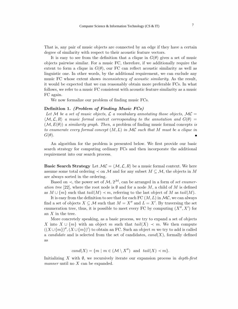
Definition 1. (Problem of Finding Music FCs)Let M be a set of music objects, L a vocabulary annotating those objects, MC =⟨M,L, R⟩ a music formal context corresponding to the annotation and G(θ) =(M, E(θ)) a similarity graph. Then, a problem of finding music formal concepts isto enumerate every formal concept (M,L) in MC such that M must be a clique inG(θ).
An algorithm for the problem is presented below. We first provide our basicsearch strategy for computing ordinary FCs and then incorporate the additionalrequirement into our search process.
Basic Search Strategy Let MC = ⟨M,L, R⟩ be a music formal context. We hereassume some total ordering ≺ on M and for any subset M ⊆ M, the objects in Mare always sorted in the ordering.
Based on ≺, the power set of M, 2M, can be arranged in a form of set enumer-ation tree [22], where the root node is ∅ and for a node M , a child of M is definedas M ∪ {m} such that tail(M) ≺ m, referring to the last object of M as tail(M).
It is easy from the definition to see that for each FC (M,L) inMC, we can alwaysfind a set of objects X ⊆ M such that M = X ′′ and L = X ′. By traversing the setenumeration tree, thus, it is possible to meet every FC by computing (X ′′, X ′) foran X in the tree.
More concretely speaking, as a basic process, we try to expand a set of objectsX into X ∪ {m} with an object m such that tail(X) ≺ m. We then compute((X∪{m})′′, (X∪{m})′) to obtain an FC. Such an object m we try to add is calleda candidate and is selected from the set of candidates, cand(X), formally definedas
cand(X) = {m | m ∈ (M\X ′′) and tail(X) ≺ m}.
Initializing X with ∅, we recursively iterate our expansion process in depth-firstmanner until no X can be expanded.
Computer Science & Information Technology (CS & IT) 7

It is noted that based on the ordering ≺, we can avoid a considerable numberof duplicate generations of each individual FC.
More concretely speaking, when we expand X with a candidate m ∈ cand(X),if (X ∪ {m})′′ \ X ′′ includes some object x such that x ≺ m, then the FC ((X ∪{m})′′, (X ∪ {m})′) and those obtained from any descendant of X ∪ {m} are com-pletely useless because those concepts have already been obtained in our depth-firstsearch. Therefore, we can immediately stop further expansions of X ∪ {m} andbacktrack to the next candidate.
Pruning Useless Music FCs According to the basic strategy, we can surelyextract every ordinary FC in MC. Since our final goal is to find every FC whoseextent must form a clique in G(θ), we incorporate the requirement into our searchprocess.
As a simple observation, it is easy to see that any subset of a clique in G(θ)is also a clique. This implies that if a set of music objects X ⊆ M cannot form aclique in G(θ), any superset of X can never be a clique. This observation brings usa simple pruning rule we can enjoy during our search process.
For an (ordinary) FC MC, if its extent does not form a clique, then any FCssucceeding to MC in our depth-first search tree can safely be pruned as useless onesbecause their extents do not also form cliques and therefore can never be our targetFCs. Whenever we find such a violation of the requirement, we can immediatelystop our expansion process and then backtrack.
Algorithm Description We present a simple depth-first algorithm for findingour target music FCs. Its pseudo-code is shown in Figure 2.
In the figure, the head (first) element of a set S is referred to as head(S).Moreover, we refer to the original index of object o in OMC as index(o). Theif statement at the beginning of procedure FCFind is for avoiding duplicategenerations of the same FC and the else if for pruning useless expansions.
5 Experimental Results
In this section, we present our experimental results. We have implemented ouralgorithm for finding music formal concepts consistent with audio features andconducted several experimentations to verify its usefulness. Our system has beencoded in C and executed on a PC with IntelR⃝ Core
TMi5 (1.6 GHz) processor and
16 GB main memory.
Computer Science & Information Technology (CS & IT)8

[Input] MC = ⟨M,L, R⟩ : a music formal contextG : a similarity graph forM based on acoustic feature vectors
[Output]MFC : the set of music formal concepts consistent withacoustic feature similarity
procedure Main(MC, G) :MFC ← ∅ ;Fix a total ordering ≺ onM ;C ←M ;while C = ∅ dobeginm← head(C) ;C ← (C \ {m}) ;MusicFCFind({m}, ∅, C) ;
endreturn FC ;
procedure MusicFCFind(X, PrevExt, Cand) :MFC ← (Ext = X ′′, X ′) ; // music FCif ∃x ∈ (Ext \ PrevExt) such that x ≺ tail(X) thenreturn; // discard duplicate music FC
else if Ext is not a clique in G thenreturn; // discard music FC violating cliqueness
endifMFC ←MFC ∪ {MFC} ;while Cand = ∅ dobeginm← head(Cand) ;Cand← Cand \ {m} ; // removing m from Cand ;NewCand← Cand \ PrevExt ; // new candidate objects.if NewCand = ∅ then continue ;MusicFCFind(X ∪ {m}, Ext, NewCand) ;
end
Fig. 2. Algorithm for Finding Music Formal Concepts Consistent with Acoustic Feature Similarity
5.1 Dataset
In our experimentation, we have used “The MagnaTagATune Dataset” [9], a datasetpublicly available 1.
The dataset contains 25,863 audio clips in MP3 format, where each of the clipshas length of 30 seconds. The number of the original music works (titles) fromwhich those clips have been extracted is 6385.
For most of the clips, two kinds of audio features, pitch and timbre, have alreadybeen provided in the dataset. More concretely speaking, for each audio clip, a coupleof sequences (time-series) of 12-dimensional vectors have been prepared for bothaudio features.
1 http://mirg.city.ac.uk/codeapps/the-magnatagatune-dataset
Computer Science & Information Technology (CS & IT) 9

The dataset also contains annotation data for the audio clips. Each of the clipsexcept for 4,221 has been annotated with several tags out of 188 possible ones.
5.2 Music Formal Context and Similarity Graphs
For preparation of our music formal context and similarity graphs for audio features,we have to select only audio clips from the dataset each of which is assigned at leastone annotation tag and has its corresponding feature vectors. We have found 21,618audio clips out of 25,863 satisfying the conditions.
Based on the selected 21,618 music audio clips and their annotation data, wehave created our music formal context MC = ⟨M,A, R⟩, where M is the set of21,618 audio clips as our data objects and A the set of 188 possible annotationtags as our attributes. Furthermore, R is defined as R = {(m, a) | m ∈ M, a ∈A,m is annotated with a}.
Our similarity graphs for audio features have also been created from the selected21,618 audio clips and their audio feature vectors. As has been stated above, eachaudio clip has its corresponding two time-series of 12-dimensional feature vectorsfor pitch and timbre. As standard processing for (music) audio data, we averageeach dimension of time-series to get a single feature vector. Moreover, we alsocompute standard deviation of each dimension. Thus, for each audio clip mi ∈ M,we can obtain four single 12-dimensional vectors, vp-avg
i , vp-stdi , vt-avg
i and vt-stdi , for
averaged pitch, standard deviation of pitch, averaged timbre and standard deviationof timbre, respectively.
Assuming M as the set of vertices, given a threshold θ for similarity of audiofeatures, our similarity graph for averaged pitch, denoted by Gp-avg(θ), has beenconstructed as Gp-avg(θ) = (M, Ep-avg(θ)), where Ep-avg(θ) is defined with vectorsvp-avgi according to the equations (1) and (2). As similarity graphs for standard
deviation of pitch, averaged timbre and standard deviation of timbre, we can con-struct Gp-std(θ), Gt-avg(θ) and Gt-std(θ), respectively, in the same manner.
We have set θ to each value in the range from 0.9 to 1.0 with a step of 0.01.
5.3 Examples of Music Formal Concepts
We present here two music formal concepts. One is an example of our target FCs ac-tually extracted by the proposed system and the other a negative example rejecteddue to inconsistency of acoustic similarity.
In Figure 3(a), we present a music FC actually found as accepted one. The FCsatisfies the requirement of acoustic similarity based on standard deviation of pitch,where θ has been set to 0.95.
The extent consists of 6 music objects all of which are annotated with (at least)the 6 tags in the intent, where each object is expressed in the form of“Artist-AlbumTitle-TrackNum-TackTitle.” Listening to those music objects, it is
Computer Science & Information Technology (CS & IT)10
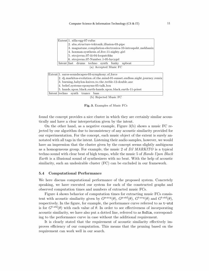
Extent 1. zilla-egg-07-rufus2. aba structure-tektonik illusion-03-pipe3. magnatune compilation-electronica-10-introspekt mekhanix4. hoxman-synthesis of five-11-nighty girl5. strojovna 07-iii-04-loopatchka6. strojovna 07-Number 1-05-bycygel
Intent fast drums techno synth funky upbeat
(a) Accepted Music FC
Extent 1. saros-soundscapes-03-symphony of force2. dj markitos-evolution of the mind-01-sunset endless night journey remix3. burning babylon-knives to the treble-12-double axe4. belief systems-eponyms-05-talk box5. hands upon black earth-hands upon black earth-11-priest
Intent techno synth trance bass
(b) Rejected Music FC
Fig. 3. Examples of Music FCs
found the concept provides a nice cluster in which they are certainly similar acous-tically and have a clear interpretation given by the intent.
On the other hand, as a negative example, Figure 3(b) shows a music FC re-jected by our algorithm due to inconsistency of any acoustic similarity provided forour experimentation. For the concept, each music object of the extent is surely an-notated with all tags in the intent. Listening their audio samples, however, we wouldhave an impression that the cluster given by the concept seems slightly ambiguousas a homogeneous group. For example, the music 2 of DJ MARKITO is a typicaltechno sound with clear beat of high tempo, while the music 5 of Hands Upon BlackEarth is a illusional sound of synthesizers with no beat. With the help of acousticsimilarity, such an undesirable cluster (FC) can be excluded in our framework.
5.4 Computational Performance
We here discuss computational performance of the proposed system. Concretelyspeaking, we have executed our system for each of the constructed graphs andobserved computation times and numbers of extracted music FCs.
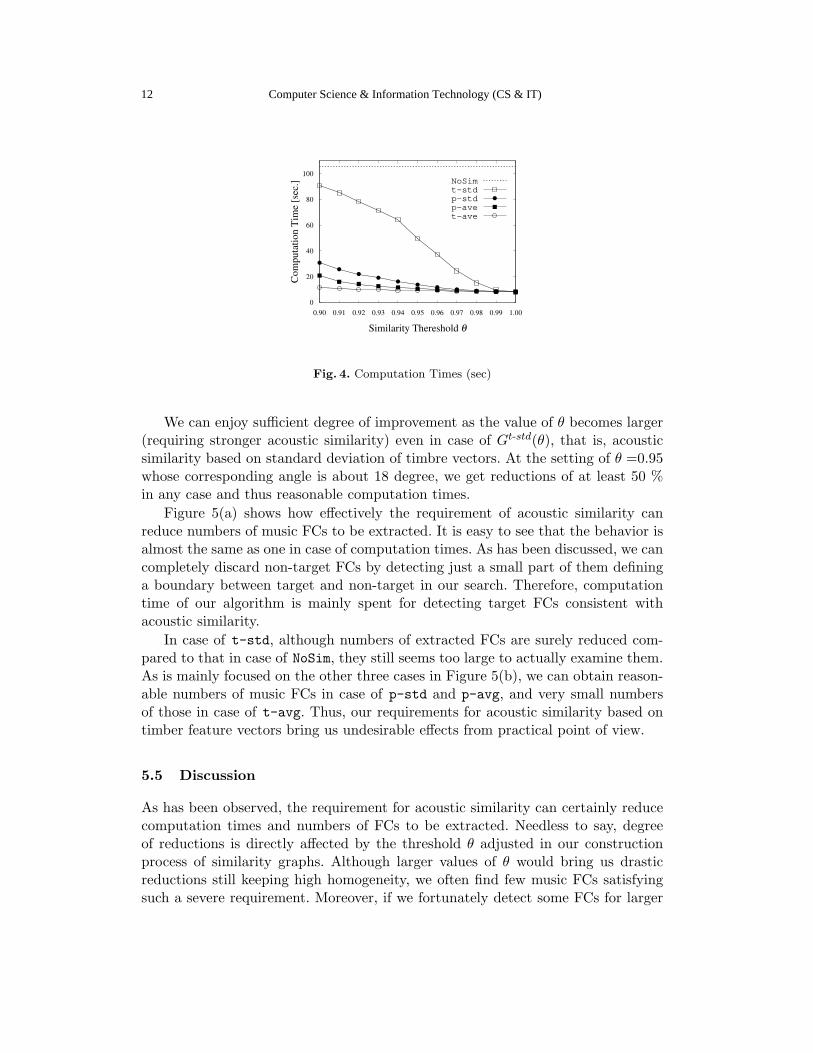
Figure 4 shows behavior of computation times for extracting music FCs consis-tent with acoustic similarity given by Gp-avg(θ), Gp-std(θ), Gt-avg(θ) and Gt-std(θ),respectively. In the figure, for example, the performance curve referred to as t-stdis for Gt-std(θ) with each value of θ. In order to see effectiveness of incorporatingacoustic similarity, we have also put a dotted line, referred to as NoSim, correspond-ing to the performance curve in case without the additional requirement.
It is clearly stated that the requirement of acoustic similarity effectively im-proves efficiency of our computation. This means that the pruning based on therequirement can work well in our search.
Computer Science & Information Technology (CS & IT) 11
0
20
40
60
80
100
0.90 0.91 0.92 0.93 0.94 0.95 0.96 0.97 0.98 0.99 1.00
Com
puta
tion T
ime
[sec
.]
Similarity Thereshold θ
NoSimt-stdp-stdp-avet-ave
Fig. 4. Computation Times (sec)
We can enjoy sufficient degree of improvement as the value of θ becomes larger(requiring stronger acoustic similarity) even in case of Gt-std(θ), that is, acousticsimilarity based on standard deviation of timbre vectors. At the setting of θ =0.95whose corresponding angle is about 18 degree, we get reductions of at least 50 %in any case and thus reasonable computation times.
Figure 5(a) shows how effectively the requirement of acoustic similarity canreduce numbers of music FCs to be extracted. It is easy to see that the behavior isalmost the same as one in case of computation times. As has been discussed, we cancompletely discard non-target FCs by detecting just a small part of them defininga boundary between target and non-target in our search. Therefore, computationtime of our algorithm is mainly spent for detecting target FCs consistent withacoustic similarity.
In case of t-std, although numbers of extracted FCs are surely reduced com-pared to that in case of NoSim, they still seems too large to actually examine them.As is mainly focused on the other three cases in Figure 5(b), we can obtain reason-able numbers of music FCs in case of p-std and p-avg, and very small numbersof those in case of t-avg. Thus, our requirements for acoustic similarity based ontimber feature vectors bring us undesirable effects from practical point of view.
5.5 Discussion
As has been observed, the requirement for acoustic similarity can certainly reducecomputation times and numbers of FCs to be extracted. Needless to say, degreeof reductions is directly affected by the threshold θ adjusted in our constructionprocess of similarity graphs. Although larger values of θ would bring us drasticreductions still keeping high homogeneity, we often find few music FCs satisfyingsuch a severe requirement. Moreover, if we fortunately detect some FCs for larger
Computer Science & Information Technology (CS & IT)12

0
10000
20000
30000
40000
50000
0.90 0.91 0.92 0.93 0.94 0.95 0.96 0.97 0.98 0.99 1.00
Num
ber
of
Extr
acte
d F
Cs
Similarity Thereshold θ
NoSimt-stdp-stdp-avet-ave
(a) Overview in Entire Range of θ
0
500
1000
1500
2000
2500
3000
0.90 0.91 0.92 0.93 0.94 0.95 0.96 0.97 0.98 0.99 1.00
Num
ber
of
Extr
acte
d F
Cs
Similarity Thereshold θ
t-std
p-std
p-ave
t-ave
(b) Details in Lower-Range
Fig. 5. Number of Extracted Music Formal Concepts
θ, they would not be interesting for us in the sense that such an FC tends to includemany music objects by the same artist or in the same album 2. Therefore, we haveto carefully set θ to an adequate value. At the moment, we have just an empiricalinstruction that values around 0.95 would be reasonable from practical viewpoint.
As an extended approach, users can flexibly adjust values of θ with the helpof user-interaction so that they can intensively and deeply examine music FCsparticularly interesting for them. At an early stage, we try to extract music FCs bysetting θ to a (relatively) small value. In such a setting, since the requirement foracoustic similarity is not severe, it is easy to imagine that we have a large numberof FCs. Obviously, showing users all of them is quite impractical. In order to havean overview of our music database, it would be reasonable to present maximallygeneral FCs (that is, ones with maximally larger extents) which have a very smallpart of them. Browsing those maximal FCs, users would mark several promisingcandidates to further examine. For an increased value of θ, we can again extractmusic FCs with finer homogeneity and then intensively find ones related to thecandidates previously marked.
6 Concluding Remarks
In this paper, we discussed a method of finding music formal concepts. Those con-cepts correspond to meaningful clusters of music objects in the sense that eachcluster can clearly be interpreted in terms of its intent and consists of objectsacoustically similar. We presented a depth-first algorithm for efficiently extractingmusic FCs with a simple pruning rule. In our experimentations, we observed use-
2 In case where several music objects are clipped from a single track, as The MagnaTagATuneDataset, we could find most of the objects in an FC are from the same track.
Computer Science & Information Technology (CS & IT) 13

fulness of the proposed method from the viewpoints of quality of extracted FCsand computational efficiency.
Since our current framework assumes that each music object is assigned its ownlinguistic information like annotation-tags, we have to cope with issues such as coldstart problems in recommendation systems. It would be worth incorporating somemechanism of automatic-tagging/labeling into our current system.
The proposed method is a general framework applicable to any domain in whichdata objects can be represented in numerical vectors and assigned their own lin-guistic information. Based on the current framework, we can design and developuseful recommendation systems in various application domains.
References
1. L. Billard ad E. Diday. Symbolic Data Analysis, Wiley, 2006.2. S. Marsland, Machine Learning: An Algorithmic Perspective, Second Edition, CRC Press,
2015.3. Y. V. S. Murthy and S. G. Koolagudi. Content-Based Music Information Retrieval (CB-MIR)
and Its Applications toward the Music Industry: A Review, ACM Computing Surveys, 51(3),Article 45, 2018.
4. T. Li, M. Ogihara and G. Tzanetakis (eds.). Music Data Mining, CRC Press, 2012.5. D. Paul and S. Kundu. A Survey of Music Recommendation Systems with a Proposed Music
Recommendation System, Emerging Technology in Modelling and Graphics, AISC-937, pp. 279– 285, Springer, 2020.
6. Y. Song, S. Dixon and M. Pearce. A Survey of Music Recommendation Systems and FuturePerspectives, In Proc. of the 9th Int’l Symp. on Computer Music Modeling and Retrieval -CMMR’12, pp. 395 – 410, 2012.
7. D. Lin and S. Jayarathna. Automated Playlist Generation from Personal Music Libraries, InProc. of 2018 IEEE Int’l Conf. on Information Reuse and Integration for Data Science, pp.217 – 224, 2018.
8. F. Morchen, A. Ultsch, M. Nocker and C. Samm. Visual Mining in Music Collections, FromData and Information Analysis to Knowledge Engineering, M. Spiliopoulou, R. Kruse, C.Borgelt, A. Nurnberger and W. Gaul (eds.), pp. 724 – 731, Springer, 2006.
9. E. Law, K. West, M. Mandel, M. Bay and J. S. Downie. Evaluation of Algorithms UsingGames: The Case of Music Tagging, In Proc. of the 10th Int’l Conf. on Music InformationRetrieval - ISMIR’09, pp. 387 – 392, 2009.
10. P. Knees and M. Schedl. A Survey of Music Similarity and Recommendation from Music Con-text Data, ACM Transactions on Multimedia Computing, Communication and Applications,10(1), Article 2, 2013.
11. F. Pachet. Knowledge Management and Musical Metadata, In Encyclopedia of KnowledgeManagement, 2005.
12. D. Wang, T. Li and M. Ogihara. Are Tags Better Than Audio Features? The Effect of JointUse of Tags and Audio Content Features for Artistic Style Clustering, In Proc. of the 11thInt’l Society for Music Information Retrieval Conference - ISMIR’10, pp. 57 – 62, 2010.
13. R. Miotto and N. Orio. A Probabilistic Model to Combine Tags and Acoustic Similarity forMusic Retrieval, ACM Transactions on Information Systems, 30(2), Article 8, 2012.
14. P. Knees, T. Pohle, M. Schedl, D. Schnitzer, K. Seyerlehner and G. Widmer. AugmentingText-Based Music Retrieval with Audio Similarity, In Proc. of the 10th Int’l Society for MusicInformation Retrieval Conference - ISMIR’09, pp. 579 – 584, 2009.
Computer Science & Information Technology (CS & IT)14

15. A. Ahmad and S. S. Khan. Survey of State-of-the-Art Mixed Data Clustering Algorithms,IEEE Access, 7, pp. 31883 – 31902, 2019.
16. K. M. Ibrahim, J. Royo-Letelier, E. V. Epure, G. Peeters and G. Richard. Audio-Based Auto-Tagging With Contextual Tags for Music, In Proc. of 2020 IEEE International Conference onAcoustics, Speech and Signal Processing - ICASSP 2020, pp. 16 – 20, 2020.
17. L. Kumar A. Mitra, M. Mittal, V. Sanghvi, S. Roy and S. K. Setua. Music Tagging and Similar-ity Analysis for Recommendation System, Computational Intelligence in Pattern Recognition,AISC-999, pp 477 – 485, Springer, 2020.
18. D. Turnbull, L. Barrington and G. Lanckriet. Five Approaches to Collecting Tags for Music,In Proc. of the 9th Int’l Society for Music Information Retrieval Conference - ISMIR’08, pp.225 – 230, 2008.
19. B. Ganter and R. Wille. Formal Concept Analysis – Mathematical Foundations, 284 pages,Springer, 1999.
20. B. Ganter, G. Stumme and R. Wille (Eds). Formal Concept Analysis – Foundations andApplications, LNAI-3626, 348 pages, Springer, 2005.
21. P. Knees and M. Schedl. Music Similarity and Retrieval, Springer, 2016.22. R. Rymon. Search through Systematic Set Enumeration, In Proc. of Int’l Conf. on Principles
of Knowledge Representation Reasoning - KR’92, pp. 539 – 550, 1992.
Computer Science & Information Technology (CS & IT) 15
© 2020 By AIRCC Publishing Corporation. This article is published under the Creative CommonsAttribution (CC BY) license.

16 Computer Science & Information Technology (CS & IT)
David C. Wyld et al. (Eds): COMIT, SIPO, AISCA, MLIOB, BDHI - 2020
pp. 17-25, 2020. CS & IT - CSCP 2020 DOI: 10.5121/csit.2020.101602
CONCATENATION TECHNIQUE IN CONVOLUTIONAL NEURAL
NETWORKS FOR COVID-19 DETECTION
BASED ON X-RAY IMAGES
Yakoop Razzaz Hamoud Qasim Habeb Abdulkhaleq Mohammed Hassan
Abdulelah Abdulkhaleq Mohammed Hassan
Department of Mechatronics and Robotics Engineering,
Taiz University, Yemen
ABSTRACT In this paper we present a Convolutional Neural Network consisting of NASNet and MobileNet
in parallel (concatenation) to classify three classes COVID-19, normal and pneumonia,
depending on a dataset of 1083 x-ray images divided into 361 images for each class. VGG16
and RESNet152-v2 models were also prepared and trained on the same dataset to compare
performance of the proposed model with their performance. After training the networks and
evaluating their performance, an overall accuracy of 96.91%for the proposed model, 92.59%
for VGG16 model and 94.14% for RESNet152. We obtained accuracy, sensitivity, specificity
and precision of 99.69%, 99.07%, 100% and 100% respectively for the proposed model related
to the COVID-19 class. These results were better than the results of other models. The
conclusion, neural networks are built from models in parallel are most effective when the data
available for training are small and the features of different classes are similar.
KEYWORDS Deep Learning, Concatenation Technique, Convolutional Neural Networks, COVID-19,
Transfer Learning.
1. INTRODUCTION In late 2019, a new strain of coronavirus emerged and was named coronavirus disease 2019
(COVID-19), and the first case of COVID-19 infection was registered in Wuhan, China [1], there
are many symptoms that appear on a person with COVID-19 such as fever, cough, cold ,shortness ordifficulty in breathing, problems in respiratory systems and pain in the joints[2].
According to The World Health Organization(WHO) the number of deaths by COVID-19 has
exceeded 506 thousand, the number of confirmed cases has reached over 10 million and the
number of recovery cases has reached 5.24 million[3]. Given the rapid spread of COVID-19 and its devastating effects on the lifestyle of people and their lives, countries resorted to applying the
general quarantine to stop the spread of COVID-19, which led to catastrophic consequences for
countries economy, so it was necessary to develop means to detect COVID-19, because early and wide detection means reducing the spread of the disease. According to WHO, the respiratory tract
infection, specifically the lung infection is considered one of signs and symptoms of COVID-
19[3].

18 Computer Science & Information Technology (CS & IT)
As is well known, a radiological diagnosis X-Ray and CT images can be used to detect and diagnose respiratory problems, and using radiological diagnosis, this helps to overcome the
shortage and scarcity of the examination tools and allowing to examine the largest possible
population for the availability of radiological diagnostic devices in most hospitals and
laboratories. But there is a disadvantage in radiological diagnosis, due to the necessity of needing an expert in radiology to confirm and diagnose the disease, which leads again to slowing the
process of diagnosis and increase the cost, so the approach suggested in this paper is to use deep
Convolutional Neural Network (CNN) to diagnose and detect COVID-19.The model we proposed is a CNN model which is based on the concatenation of NASNet-Mobile [4] and
MobileNet [5] for classified three classes COVID-19, normal and pneumonia.
2. RELATED WORK To diagnose COVID-19 disease by using convolutional neural network CNN based on X-ray
images, several searches have been introduced in this field.In [6] the authors used a network
consisting of Xception [7] and ResNet50-v2 [8] in parallel on a dataset of 15085X-ray images. They used a cross validation strategy to training the network, this proposed model achieved an
average overall accuracy of 94.4%. In [9] the authors presented a CNN model named nCOVNet
which is based on the VGG19 model [10], transfer learning was used to retrain the model on a dataset consisting of 284 X-ray images for the two classes COVID-19 and normal. After training
the model achieved an overall accuracy of 88.10%, sensitivity of 97.62% and specificity of
78.57%. In [11] the authors presented a CNN model called CoroNet based on Xception
architecture. The model was trained on a dataset consisting of 1251 X-ray images for four classes COVID-19, normal, bacterial pneumonia and viral pneumonia. The model achieved an overall
accuracy of 89.69%, specificity of 93% and 98.2% related to the COVID-19 class. The model
was also trained in three classes COVID-19, normal and pneumonia (mixture of viral and bacterial), and obtained an overall accuracy of 95%. In [12] the authors used transfer learning
technique to train the VGG19model on a dataset of 445 X-ray images for COVID-19 and normal
classes. They achieved an overall accuracy of 96.3%, sensitivity of 97% and precision of 91.7% related to the COVID-19 class. In [13] transfer learning technology was used to train VGG19
[10], MobileNet-v2 [14], Inception [15], Xception [7] and Inception ResNet-v2 [16] on a dataset
consisting of 1428 X-ray images for three classes COVID-19, normal and bacterial pneumonia,
They got 99.10% sensitivity for COVID-19 class from MobileNet model. After that, a group of X-ray images of viral pneumonia was added to the previous dataset and then trained on
MobileNet model, the model achieved an overall accuracy of 94.72% and 96.78% accuracy for
the COVID-19 class.
The remainder of this paper can be summarized as follows. In section three we explain the
methodology which consists of the proposed model and the dataset which is used for training the
model, then in section four we will show the results we obtained from the proposed model and other models, then in section five we will discuss the results and in section six we will show the
conclusion that we reached.
3. METHODOLOGY
3.1. Dataset Due to the lack of available resources for chest X-ray images of those people with COVID-19,
the dataset that is used in this paper were collected from several sources. The first source which is
COVID-19 image data collection [17],is available on GitHub website and only 142 images were taken for COVID-19 class. The second source which is COVID-19 Radiography database[18], is

Computer Science & Information Technology (CS & IT) 19
available on Kaggle website, contains 219 cases for COVID-19, 1341 normal and 1345 for viral pneumonia, all images from COVID-19 cases were taken as well as 361 from normal cases. The
third source which is chest x-ray images (pneumonia) [19],is available on Kaggle website,
contains 5863 x-ray images for two classes normal and pneumonia(a mixture of viral and
bacterial),and 361 cases were taken for the pneumonia class. After collecting the images from the three sources, we had 1083 images divided into 316 images for each class. We divided the dataset
into 759 images for training and 324 for validation. We did not perform any process to check the
accuracy of the data, we satisfied with the reliability of the sources and the data was divided randomly.
3.2. Convolutional Neural Network
Convolutional neural network (CNN) is type of neural network which is very effective in the
field of image classification and problem solving of image processing. The word convolution refers to the filtering process that happen in this type of networks [20]. This networks consist of
multiple layers which are: The convolution layer which is the core layer and it works by placing a
filter over an array of image pixels, this then creates what is known as a Convolved Feature Map (CFM). The pooling layer which reduces the sample size of feature map, this makes processing
too faster [20], by reducing the parameters that the network needs to process. A Rectified Linear
Unit Layer (Relu) that acts as an activation function ensuring Non-Linearity. A Fully Connected
Layer allowing us to perform classification on our dataset.
COVID-19 symptoms are often identical to the symptoms of other viral pneumonia and because
of the similarity of the effect of COVID-19 and the effect of the other infections on the lung [21, 22]. It is difficult to diagnose with X-Ray images except by an experienced X-Ray expert. But is
easier to diagnose with the neural networks. With the great similarity between the effect of
COVID-19 and other pneumonia, such as viral pneumonia, it is necessary to build a deeper neural network in order to be able to classify properly, but this type of network requires a large dataset
and high computing capabilities for training. Whereas building a network of two models in
parallel has the ability to learn different and overlapping high-level and low-level features [23].
So we built a network of two models in parallel (concatenation) to have a high ability to extract
and classify features properly, so we used NASNet-Mobile [4] and MobileNet [5] to configure
this network. NASNet-Mobile was chosen for several reasons, including the small number of parameters as well as the ability to achieve state-of-the-art result and less complexity [4, 24].
MobileNet was also chosen for several reasons, including the small size and lack of complexity
in it’s structure because it is based on the DepthWise Separable Convolution [5, 25].As noted in
figure.1, global average pooling, global max pooling and flatten have been linked in parallel to improve the network performance and help to prevent overfitting and create a feature map for
each category in the last layers [26]. To compare the performance of the proposed network, two
models VGG16 [27] and RESNET152-v2 [28] were prepared and trained on the same dataset. These two models are the most popular used. The VGG16 model is very popular and widely used
because of pre-trained weights were made freely available online. RESNET152-v2 also is one of
the most popular models which "introduced the concept of Residual Learning in which the subtraction of features is learned from the input layer by using shortcut connection"[29].

20 Computer Science & Information Technology (CS & IT)
Figure. 1. The architecture of the proposed network, concatenation of two models
3.3. Transfer Learning
A technique for reusing the weights of pre-trained network on a task similar to the current task as classification. We have used this technique to train all previously mentioned models, which
makes it easier for us to train new models in less time and few computing resource.
Table 1 Training Hyper-Parameters.
Hyper-
Parameters
Models
VGG16 ResNet152 Proposed
Batch Size 32 32 32
Learning Rate 1e-3 1e-3 1e-3
Epochs 50 30 30
Image Size 200,200 200,200 200,200
Optimizer Function
Adam Adam SGD
Data
Augmentation No No No
Loss Function Categorical-crossentropy
Categorical-crossentropy
Categorical-crossentropy
Validation
Split 0.30 0.30 0.30
4. RESULTS
After the training the models and evaluating their performance with confusion matrix we
obtained the following results.
Computer Science & Information Technology (CS & IT) 21
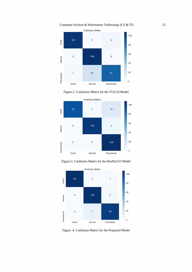
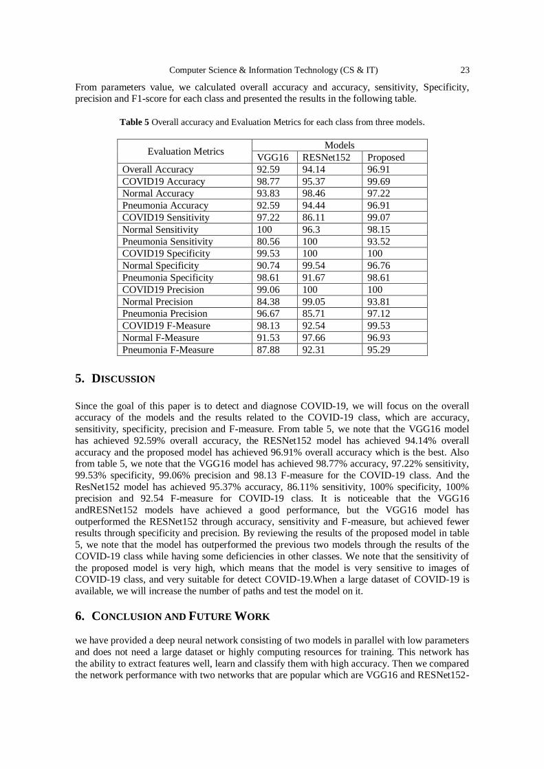
Figure.2. Confusion Matrix for the VGG16 Model
Figure.3. Confusion Matrix for the ResNet152 Model
Figure. 4. Confusion Matrix for the Proposed Model

22 Computer Science & Information Technology (CS & IT)
Confusion Matrix is a matrix that is used for describing the performance of the classification model on a set of validation data whose true values are already known, confusion matrix is useful
for measuring accuracy, sensitivity, specificity, precision and F-Measure. To calculate these
values it is necessary to know four parameters which are True Positive (TP), True
Negative(TN),False Positive (FP) and False Negative(FN) and how to compute them, Suppose we wanted to calculate the four parameters mentioned previously for one of the classes and let’s
assume that the class isCOVID-19. So we have as follows.
TP: refers to the cases that belong to the COVID-19 cases and were classified under COVID-19
cases. TN: refers to the cases that belong to the other cases normal and pneumonia, and were not
classified under COVID-19 cases, FP: refers to the cases that belong to the other cases and were classified under COVID-19 cases and FN: refers to the cases that belong to COVID-19 cases and
were not classified under COVID-19 cases. Tables 2, 3 and 4 shows the results of the four
parameters for the three models related toCOVID-19, normal and pneumonia classes
respectively. Now based on these parameters we can calculate the following evaluation metrics which are accuracy for each class, sensitivity, specificity, precision and F-measure.
Sensitivity for COVID-19 tell us what percentage of cases with COVID-19 were correctly identified, Specificity for COVID-19 tell us what percentage of cases without COVID-19 were
correctly identified, Precision tell us what percentage of cases that actually belong to the COVID-
19 cases from all cases that classified as COVID-19. F-Measure which is the harmonic mean of sensitivity and precision.
Overall Accuracy = correct predictions / total predictions.
Accuracy for each class = (TP + TN) / (TP + FP + TN + FN) Sensitivity = TP / (TP + FN) .
Specificity = TN / (TN + FP).
Precision = TP / (TP + FP) F-Measure = 2*Sensitivity*Precision / (precision + Sensitivity)
From the previous Confusion Matrixes, we calculated the four parameters and presented
them in the following tables for each class.
Table 2 Four parameters related to the COVID-19 class.
Model TP FP TN FN
VGG16 105 1 215 3
RESNet152 93 0 216 15
Proposed 107 0 216 1
Table 3 Four parameters related to the Normal class.
Model TP FP TN FN
VGG16 108 20 196 0
RESNet152 104 1 215 4
Proposed 106 7 209 2
Table 4 Four parameters related to the Pneumonia class.
Model TP FP TN FN
VGG16 87 3 213 21
RESNet152 108 18 198 0
Proposed 101 3 213 7
Computer Science & Information Technology (CS & IT) 23
From parameters value, we calculated overall accuracy and accuracy, sensitivity, Specificity, precision and F1-score for each class and presented the results in the following table.
Table 5 Overall accuracy and Evaluation Metrics for each class from three models.
Evaluation Metrics Models
VGG16 RESNet152 Proposed
Overall Accuracy 92.59 94.14 96.91
COVID19 Accuracy 98.77 95.37 99.69
Normal Accuracy 93.83 98.46 97.22
Pneumonia Accuracy 92.59 94.44 96.91
COVID19 Sensitivity 97.22 86.11 99.07
Normal Sensitivity 100 96.3 98.15
Pneumonia Sensitivity 80.56 100 93.52
COVID19 Specificity 99.53 100 100
Normal Specificity 90.74 99.54 96.76
Pneumonia Specificity 98.61 91.67 98.61
COVID19 Precision 99.06 100 100
Normal Precision 84.38 99.05 93.81
Pneumonia Precision 96.67 85.71 97.12
COVID19 F-Measure 98.13 92.54 99.53
Normal F-Measure 91.53 97.66 96.93
Pneumonia F-Measure 87.88 92.31 95.29
5. DISCUSSION
Since the goal of this paper is to detect and diagnose COVID-19, we will focus on the overall accuracy of the models and the results related to the COVID-19 class, which are accuracy,
sensitivity, specificity, precision and F-measure. From table 5, we note that the VGG16 model
has achieved 92.59% overall accuracy, the RESNet152 model has achieved 94.14% overall
accuracy and the proposed model has achieved 96.91% overall accuracy which is the best. Also from table 5, we note that the VGG16 model has achieved 98.77% accuracy, 97.22% sensitivity,
99.53% specificity, 99.06% precision and 98.13 F-measure for the COVID-19 class. And the
ResNet152 model has achieved 95.37% accuracy, 86.11% sensitivity, 100% specificity, 100% precision and 92.54 F-measure for COVID-19 class. It is noticeable that the VGG16
andRESNet152 models have achieved a good performance, but the VGG16 model has
outperformed the RESNet152 through accuracy, sensitivity and F-measure, but achieved fewer results through specificity and precision. By reviewing the results of the proposed model in table
5, we note that the model has outperformed the previous two models through the results of the
COVID-19 class while having some deficiencies in other classes. We note that the sensitivity of
the proposed model is very high, which means that the model is very sensitive to images of COVID-19 class, and very suitable for detect COVID-19.When a large dataset of COVID-19 is
available, we will increase the number of paths and test the model on it.
6. CONCLUSION AND FUTURE WORK
we have provided a deep neural network consisting of two models in parallel with low parameters
and does not need a large dataset or highly computing resources for training. This network has
the ability to extract features well, learn and classify them with high accuracy. Then we compared the network performance with two networks that are popular which are VGG16 and RESNet152-

24 Computer Science & Information Technology (CS & IT)
v2 in terms overall accuracy, accuracy for each class, sensitivity, specificity and F-measure. The result of this network were very good and satisfactory compared to the result obtained from other
networks. Thus we come to conclusion that the neural networks in this way are very effective in
the event that the available dataset are few, and there is a great similarity in the features between
the classes. In the future works, we will test the model on a different dataset and develop the model so that it is very effective in medical diagnostics.
REFERENCES [1] N. Zhu, D. Zhang, W. Wang, X. Li, B. Yang, J. Song, X. Zhao, B. Huang, W. Shi, R. Lu, P. Niu, F.
Zhan, X. Ma, D. Wang, W. Xu, G. Wu, G.F. Gao, W. Tan, A novel coronavirus from patients with
pneumonia in China, 2019 N. Engl. J. Med., 382 (2020), pp. 727-733
[2] C. Huang, Y. Wang, X. Li, L. Ren, J. Zhao, Y. Hu, L. Zhang, G. Fan, J. Xu, X. Gu, Z. Cheng, T. Yu,
J. Xia, Y. Wei, W. Wu, X. Xie, W. Yin, H. Li, M. Liu, Y. Xiao, H. Gao, L. Guo, J. Xie, G. Wang, R.
Jiang, Z. Gao, Q. Jin, J. Wang, B. Cao, Clinical features of patients infected with 2019 novel
coronavirus in Wuhan, China Lancet, 395 (2020), pp. 497-506 [3] WHO Coronavirus disease. Last Accessed : 30 Jun 2020
[4] Barret Zoph, Vijay Vasudevan, Jonathon Shlens, Quoc V. Le. Learning Transferable Architectures for
Scalable Image Recognition. arXiv:1707.07012v4. 2018.
[5] Andrew G. Howard, Menglong Zhu, Bo Chen, Dmitry Kalenichenko, Weijun Wang, Tobias Weyand,
Marco Andreetto, Hartwing Adam. MobileNets: Efficient Convolutional Neural Networks for Mobile
Vision Application. arXiv:1704.04861v1. 2017.
[6] Mohammad Rahimzadeh, Abolfal Attar. A modified deep convolutional neural network for detecting
COVID-19 and pneumonia from X-ray images based on the concatenation of Xception and
ResNet50v2. (2020) 2020.100360.
[7] Chollet F. Xception: deep learning with depthwise separable convolution. In: proceedings pf the IEEE
conference on computer vision and pattern recognition. 2017. P. 1251-8. [8] He K, Zhang X, Ren S, Sun J. Identity mappings in deep residual networks. In:European conference
on computer vision. Springer, 2016. p. 630-45.
[9] Harsh Panwar, P.K. Gupta, Mhammad Khubeb Siddiqui, Ruben Morales-Menendez, Vaishnavi
Singh. Application of deep learning for fast detection of COVID-19 in X-ray using nCOVnet. (2020)
2020.109944.
[10] Simonyan K, Zisserman A (2014) Very deep convolutional networks for large-scale image
recognition. arXiv, 1409: p. 1556.
[11] Asif Iqbal Khan, Junaid Latief Shah, Mohammad Mudasir Bhat. CoroNet: A deep neural network for
detection and diagnosis of COVID-19 from chest x-ray images. (2020) 2020.105581.
[12] Shahank Vaid, Reza Kalantar, Mohit Bhandari. Deep learning COVID-19 detection bias: accuracy
through artificial intelligence. 2020. https://doi.org/10.1007/s00264-020-04609-7.
[13] Ioannis D. Apostolopoulos, Tzani A. Mpesiana. Covid-19: Automatic detection from X-ray images utilizing transfer learning with convolutional neural networks. 2020. https://doi.org/10.1007/s13246-
020-00865-4.
[14] Howard AG Zhu M Chen B et al (2017)MobileNets: efficient convolutional neural networks for
mobile vision applications. arXiv preprint arXiv: 170404861.
[15] Szegedy C, Liu W, Jia Y, Sermanet P, Reed S, Anguelov D, et al. Going deeper with
convolutions.Boston, MA, 2015,: IEEE Conference on Computer Vision and Pattern Recognition
(CVPR); 2015. P. 1-9.
[16] Szegedy C, Ioffe S, Vanhoucke V, Alemi A. Inception-v4, inception-resnet and the impact of residual
connections on learning. 2016.
[17] Cohen JP. COVID-19 image data collection. (2020) https://github.com/ieee8023/covid-chestxray-
dataset. [18] Tawsifur Rahman, M.E.H. Chowdhury, A. Khandakar. COVID-19 Radiography database.
https://www.kaggle.com/tawsifurrahman/covid19-radiography-database .
[19] Paul Mooney. Chest X-ray Images (Pneumonia). https://www.kaggle.com/paultimothymooney/chest-
xray-pneumonia .

Computer Science & Information Technology (CS & IT) 25
[20] Sumit Saha. A Comprehensive Guide to Convolutional Neural Network –the ELI5 way.
https://towordsdatascience.com/a-comprehensive-guide-to-convolutional-neural-network-the-eli5-
way-3bd2b1164a5 . Last accessed on Jun 2020.
[21] Zawn Villines. What is the relationship between pneumonia and COVID-19?.
https://www.medicalnewstoday.com/articles/pneumonia-and-covid-19#summary . last accessed on Jun 2020.
[22] Jill Seladi-Schulman. What to Know About COVID-19 and Pneumonia .
https://www.healthline.com/health/coronavirus-pneumonia. Last accessed on Jun 2020.
[23] Sabyasachi Sahoo. Grouped Convolutiona – convolutions in parallel.
https://towordsdatascience.com/grouped-convolutions-convolutions-in-parallel-3b8cc847e851 . Last
accessed on May 2020.
[24] Sik-Ho Tsang. Review: NASNet-Neural Architecture Search Network (Image Classification).
https://medium.com/@sh.tsang/review-nasnet-neural-architecture-search-network-image-
classification-23139ea0425d . Last accessed on APRIL 2020.
[25] Sik-Ho Tsang. Review:MobileNetv1-Depthwise Separable Convolution (Light Weight Model).
https://towardsdatascience.com/review-mobilenetv1-depthwise-separable-convolution-light-weight-
model-a382df364b69 . Last accessed MAY 2020. [26] Chris. What are Max Pooling, Average Pooling, Global Max Pooling and Global Average Pooling.
https://www.machinecurve.com/index.php/2020/01/30/what-are-max-pooling-average-pooling-
global-max-pooling-and-global-average-pooling/ . Last accessed on MARCH 2020.
[27] Karen Simonyan, Andrew Zisserman. Very Deep Convolutional Networks for Large-Scale Image
Reconition. arXiv:1409.1556. 2014.
[28] Kaiming He, Xiangyu Zhang, Shaoqing Ren, Jian Sun. Deep Residual Learning for Image
Recognition. arXiv:1512.03385. 2015.
[29] Han, Seung & Park, Gyeong & Lim, Woohyung & Kim, Myoung & Na, Jung-Im & Park, Ilwoo &
Chang, Sung. (2018). Deep neural networks show an equivalent and often superior performance to
dermatologists in onychomycosis diagnosis: Automatic construction of onychomycosis datasets by
region-based convolutional deep neural network. PLOS ONE. 13. e0191493. 10.1371/journal.pone.0191493.
AUTHORS
Yakoop Qasim A student in the fourth level, department of Mechatronics and Robotics
Engineering , Al-Saeed college of Engineering and Information Technology at Taiz
University. Professional in designing control systems, modeling and simulation of
dynamic systems. Intelligent system programmer and interested in the field of artificial
intelligence.
Habeb Hassan A student in the fourth level, department of Mechatronics and Robotics Engineering , Al-Saeed college of Engineering and Information Technology at Taiz
University. Have many skills in programming and designing, hope in the future to
prepare master’s degree in artificial intelligence and how to use it in robotics.
Abdulelah Hassan A student in the third level, department of Mechatronics and
Robotics Engineering , Al-Saeed college of Engineering and Information Technology at
Taiz University.
© 2020 By AIRCC Publishing Corporation. This article is published under the Creative Commons
Attribution (CC BY) license.

26 Computer Science & Information Technology (CS & IT)

David C. Wyld et al. (Eds): COMIT, SIPO, AISCA, MLIOB, BDHI - 2020
pp. 27-39, 2020. CS & IT - CSCP 2020 DOI: 10.5121/csit.2020.101603
A GRID-POINT DETECTION
METHOD BASED ON U-NET FOR A
STRUCTURED LIGHT SYSTEM
Dieuthuy Pham1, 2, Minhtuan Ha1, 2 and Changyan Xiao1
1College of Electrical and Information Engineering,
Hunan University, Changsha 410208, China 2Faculty of Electrical Engineering, Saodo University,
Haiduong 170000, Vietnam
ABSTRACT Accurate detection of the feature points of the projected pattern plays an extremely important
role in one-shot 3D reconstruction systems, especially for the ones using a grid pattern. To solve this problem, this paper proposes a grid-point detection method based on U-net. A specific
dataset is designed that includes the images captured with the two-shot imaging method and the
ones acquired with the one-shot imaging method. Among them, the images in the first group
after labeled as the ground truth images and the images captured at the same pose with the one-
shot method are cut into small patches with the size of 64x64 pixels then feed to the training set.
The remaining of the images in the second group is the test set. The experimental results show
that our method can achieve a better detecting performance with higher accuracy in
comparison with the previous methods.
KEYWORDS Feature point detection, U-net architecture, Structured light system & Grid pattern
1. INTRODUCTION
One-shot structured light methods are being more and more developed since its advantages in terms of reconstructing the dynamic scene. Besides, these methods are also very economical and
easy to do with just one camera and one projector. Firstly, a well-coded pattern is projected onto
the scene. Then the image of the deformed pattern captured by the camera is fed into a decoding program to find correspondence points in the projector image plane and the camera image plane.
With the points obtained, the triangulation method will be performed to find the 3D points in the
point cloud. Although these methods cannot provide a dense 3D map with high accuracy as the
multi-shot ones, it still satisfies the requirements of many applications in reality.
Up to now, numerous one-shot imaging methods have been proposed with different pattern
coding strategies and achieved some achievements [1]. A multi-stripe pattern with De Bruijn sequence single-axis coded is proposed in [2]. With the constraint that two consecutive stripes
cannot share the same color channel, so many color channels are required for a large resolution of
the pattern. In this method, the pixels on the centerline of the color stripes are taken as feature
points, thus the 3D maps are highly dense. However, it is sensitive to color noise and improper to reconstruct the dynamic scene. Lei et al. [3] introduced a 6-symbol M-array pattern designed with
a 3 x 3 property window directly driven by the Hamming distance. The symbols are classified
28 Computer Science & Information Technology (CS & IT)
according to their geometrical feature and their centers are selected as feature points. With the advantage of using a binary pattern, this method can capture colorful objects and solve the
discontinuity problem. Although this method is easy to decode, its drawbacks are false detection
risk and sparse 3D map. To overcome the challenges of the method using the color stripe pattern,
a pattern of the self-equalizing De Bruijn sequence, scale-space analysis, and band-pass complex Hilbert filters were introduced in [4]. With a pattern of color stripes separated by a gap that
allows two consecutive stripes to share the same color channel, the method is capable of
accurately restores the color of the stripes of the pattern deformed by the object. Therefore, this method can provide a 3D map of objects with pure color.
Besides that, the methods using a grid pattern with the intersection of the slits chosen as feature points have the great advantage of fast decoding and high accuracy in the 3D map. In [5], a De
Bruijn sequence-based grid pattern is proposed. The pattern is coded based on the De Bruijn
space with horizontal blue slits and red vertical slits. This method and the one using a binary grid
pattern introduced in [6] use the spatial constraints to detect the feature points. In [7, 8], a color grid based on the De Bruijn sequence coded in both axes is used. With the different color
channels used to encode the vertical and horizontal slit respectively, feature points are precisely
detected in the skeleton image. The entire pattern is then fully decoded using the method in [8].
Recently, with the ability of learning complex hierarchies of features from input data,
convolutional neural networks (CNNs) are applied to several fields of machine vision. Zhang in [9] succeeds in extracting the line areas from the aerial image with a Deep Residual U-Net with a
very small number of parameters compared to the conventional U-net networks. Wang et al. [10]
proposed a new framework for segmenting the retinal vessel based on the patch-based learning
strategy and dense U-net that works well with the STARE and DRIVE datasets. In 3D reconstruction, Nguyen in [11] proposed an FPP-based single-shot 3D shape reconstruction
system and conducted experiments with three different network structures: Fully convolutional
networks (FCN), Autoencoder networks (AEN), and UNet. This method can obtain a 3D depth map from its corresponding 2D image by a transformation without any extra processing.
However, this method requires a large amount of high-quality 3D ground-truth labels obtained by
a multi-frequency fringe projection profilometry technique. For improving the performance of the
3D one-shot imaging system, many CNN-based methods using a binary pattern were introduced. Tang et al. [12] proposed a pattern encoded in the 2x2 property window with eight geometries.
Elements of the deformed pattern after extracted from the image are classified with a pre-trained
CNN network. The feature point is defined as the intersection of two adjacent rhombic shapes in the property window. Furthermore, Song et al. [13] proposed a binary grid pattern embed with
eight geometric shapes. Where the feature points, which are the grid intersections, are detected by
applying a cross template over the enhanced image. After extracting based on the four feature points at the four corners around themselves, the elements of the pattern then are classified by a
pre-trained CNN model
In the 3D reconstruction methods mentioned above, most results are evaluated only on the density of the point cloud, while a few methods regard the accuracy of the corresponding points
reconstructed in the 3D map. To avoid false detection of feature points in areas with extreme
distortion, Ha et al. [8] proposed a method for detecting opened-grid-points. However, locating the position of feature points refers to the center of the opened-grid-points at such regions just
achieves an acceptable accuracy. In [14], feature points at the objects’ boundary regions detected
with a large deviation from the groundtruth that reduce the average accuracy of the reconstructed 3D map. Furukawa and Kawasaki et al. [15] proposed a method for detecting the feature points
with a pre-trained CNN model. This process is divided into two phases: detecting horizontal and
vertical lines individually and detecting feature points. However, the datasets used for training in

Computer Science & Information Technology (CS & IT) 29
both phases were manually annotated; therefore, this method is unable to achieve a high location accuracy.
To improve the location accuracy of detected feature points, in this paper we propose a novel
method of detecting the intersection points in a grid pattern based on the U-net introduced in our previous work [16]. Firstly, different objects at each pose captured with one shot and two shot
imaging methods, respectively. In the first method, a grid pattern projected onto the scene, while
the other one uses a pattern encoded in vertical and horizontal axis individually. After applying a morphological skeletonization algorithm, the pictures taken by the two-shot method will be fused
in the complete skeleton images and then selected as the groundtruth images. These images and
their corresponding gray images were taken by the one-shot method are sequentially cut into patches with the size of 64 x 64 pixels and fed to the training set, whereas, the remaining original
large images are the test set.
The remains of this paper are organized as follows. Section 2 gives an overview of the imaging system used in the article. Then, Section 3 produces the detail of the proposed method such as U-
net network architecture, data set designing, and hyperparameters setting to train the model. The
experimental results and evaluation are presented in Section 4. Finally, the conclusions and future scope of the paper are given in Section 5.
2. SYSTEM OVERVIEW
As shown in Figure 1, our system includes two main parts which are an image acquiring subsystem (IAS) and a data processing unit. In which, the IAS consists of a Daheng MER-503-
36U3C with a resolution of 2448 x 2048 pixels, a Sony IMX264 sensor, a CMOS global shutter,
36 fps, and a Canon REALiS SX7 LCoS projector with a resolution of 1400 x 1050 pixels. Meanwhile, the data processing unit is a desktop computer with an Intel Core i7-8700, 16GB
RAM, and an NVIDIA GeForce RTX 2070 graphics card. Also, two patterns based on De Bruijn
sequence coded in the vertical and horizontal direction with 127 slits and 66 slits respectively that are utilized for the two-shots imaging method. And a color grid pattern combined from those is
for the one-shot imaging method [8].
(a) (b)
Figure 1. Our experimental setup and a part of the color grid pattern are given in (a) and (b), respectively.
3. METHODOLOGY
3.1. U-Net Architecture
For traditional U-Net networks, since the output data size is smaller than the input one. The
pixels near the border of the training image are missing which leads to lost border information.
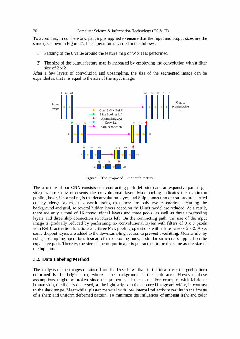
30 Computer Science & Information Technology (CS & IT)
To avoid that, in our network, padding is applied to ensure that the input and output sizes are the same (as shown in Figure 2). This operation is carried out as follows:
1) Padding of the 0 value around the feature map of W x H is performed.
2) The size of the output feature map is increased by employing the convolution with a filter size of 2 x 2.
After a few layers of convolution and upsampling, the size of the segmented image can be
expanded so that it is equal to the size of the input image.
1 64 64
64
128 128
128
256 256
256
512
512
264 64
128
128
512 256
256
256
128 1
Input
image
Output
segmentation
mapConv 3x3 + ReLU
Max Pooling 2x2
Upsampling 2x2
Conv 1x1
Skip connection
Figure 2. The proposed U-net architecture.
The structure of our CNN consists of a contracting path (left side) and an expansive path (right
side), where Conv represents the convolutional layer, Max pooling indicates the maximum pooling layer, Upsampling is the deconvolution layer, and Skip connection operations are carried
out by Merge layers. It is worth noting that there are only two categories, including the
background and grid, so several hidden layers based on the U-net model are reduced. As a result, there are only a total of 16 convolutional layers and three pools, as well as three upsampling
layers and three skip connection structures left. On the contracting path, the size of the input
image is gradually reduced by performing six convolutional layers with filters of 3 x 3 pixels
with ReLU activation functions and three Max pooling operations with a filter size of 2 x 2. Also, some dropout layers are added to the downsampling section to prevent overfitting. Meanwhile, by
using upsampling operations instead of max pooling ones, a similar structure is applied on the
expansive path. Thereby, the size of the output image is guaranteed to be the same as the size of the input one.
3.2. Data Labeling Method
The analysis of the images obtained from the IAS shows that, in the ideal case, the grid pattern
deformed is the bright area, whereas the background is the dark area. However, these assumptions might be broken since the properties of the scene. For example, with fabric or
human skin, the light is dispersed, so the light stripes in the captured image are wider, in contrast
to the dark stripe. Meanwhile, plaster material with low internal reflectivity results in the image
of a sharp and uniform deformed pattern. To minimize the influences of ambient light and color

Computer Science & Information Technology (CS & IT) 31
noise, and obtain the best data set for training, a two-shot imaging method was performed to get the label images.
As shown in Figure 3, the label set designed as follows. Firstly, objects at each pose are projected
with two patterns based on De Bruijn sequence coded in the horizontal and vertical axis, respectively. The images of the deformed pattern after captured by the camera then are applied
some preprocess techniques such as noise-reducing, blurring, and converting to HSV color space
then take the value channel as grayscale images. After that, the skeleton images, composed of horizontal and vertical lines respectively, can be obtained by applying a morphological
skeletonization algorithm to them. Finally, these images are fused and then sequentially cut into
small patches with the size of 64x64 pixels as labeled images.
Figure 3. Illustration of the data labeling process.
3.3. Data Augmentation
Our dataset consists of 20 original large grayscale images cropped to a size of 1664 x 1664 pixels
to conventional for training and testing. Among them, 13 images and their labeled ones are
sequentially cut into patches with a size of 64 x 64 pixels. So that, 676 patches are obtained from each large image. 20 % of these patches are chosen as a validation set, and the remaining ones are
the training set (Figure 4). By the data augmentation, the training set was expanded, and a new
data set of over five million training images was obtained.

32 Computer Science & Information Technology (CS & IT)
(a)
(b)
Figure 4. Illustration of the image patches of the training set. (a) Original image patches.
(b) Labeled image patches.
3.4. Parameter Settings Before putting the model into training, it is very essential to set the values of hyperparameters as
it has a significant influence on the training results. Among them, the learning rate directly affects
the learning speed of the model by regulating the intensity of the model's weighting update. If this parameter is set too small, the learning time is extended too long, on the contrary, a too-large
value can lead to an unstable learning process. In this study, by setting the learning rate to a value
of 1e-3, the network converges quickly at the point closest to the optimum one and the model can learn the detailed features in the dataset.
The batch size indicates the number of training samples utilized in one iteration. The value of this
parameter plays an important role in the convergence process of the network. A large batch size might lead the network to fall into the local minimum point and cannot converge at its optimum
point. Whereas, the network can converge at the optimal point, but this extends the training time.
The batch size used in our network is set to 128. Since an epoch consists of one full cycle through the training data, so aiming at a good training result without costing much time, the model is
trained with 100 epochs. In each epoch, the number of steps per epoch, which indicates the
number of iterations, is set to 1000. Thus, input samples are randomly selected from the above-
designed training set with the batch size for processing at each iteration.
3.5. Training and Testing Processes
During training, the samples are continuously parked with the batch size and fed to the network
from the augmented training set, where each of them consists of the sample itself and a
corresponding label image. For each filter in a layer, the network extracts several features of the input sample and transmits them to the output layer through the intermediate hidden layers.
Along with that, the value of all the elements of the weight matrix between the layers is adjusted
continuously. After training with several epochs, the value of the loss function is getting smaller and smaller and simultaneously the accuracy also gradually attains the desired value.
A block diagram of the training and testing progress for grid pattern segmentation is shown in Figure 5. Where the input samples are the patches with a size of 64 x 64 pixels drawn from the
training set and fed to the proposed CNN. The network is currently trained with such samples and
the preset hyperparameters. In each training cycle, the loss function and the accuracy are utilized
to monitor and adjust the value of the parameters for the next cycle. Finally, a high-precision segmentation model for accurately segmenting grid pattern is obtained.
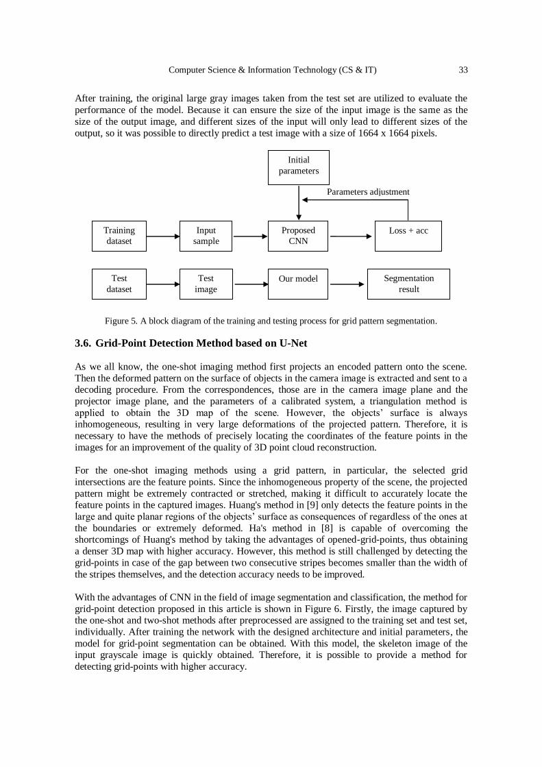
Computer Science & Information Technology (CS & IT) 33
After training, the original large gray images taken from the test set are utilized to evaluate the
performance of the model. Because it can ensure the size of the input image is the same as the
size of the output image, and different sizes of the input will only lead to different sizes of the
output, so it was possible to directly predict a test image with a size of 1664 x 1664 pixels.
Figure 5. A block diagram of the training and testing process for grid pattern segmentation.
3.6. Grid-Point Detection Method based on U-Net
As we all know, the one-shot imaging method first projects an encoded pattern onto the scene.
Then the deformed pattern on the surface of objects in the camera image is extracted and sent to a decoding procedure. From the correspondences, those are in the camera image plane and the
projector image plane, and the parameters of a calibrated system, a triangulation method is
applied to obtain the 3D map of the scene. However, the objects’ surface is always inhomogeneous, resulting in very large deformations of the projected pattern. Therefore, it is
necessary to have the methods of precisely locating the coordinates of the feature points in the
images for an improvement of the quality of 3D point cloud reconstruction.
For the one-shot imaging methods using a grid pattern, in particular, the selected grid
intersections are the feature points. Since the inhomogeneous property of the scene, the projected
pattern might be extremely contracted or stretched, making it difficult to accurately locate the feature points in the captured images. Huang's method in [9] only detects the feature points in the
large and quite planar regions of the objects’ surface as consequences of regardless of the ones at
the boundaries or extremely deformed. Ha's method in [8] is capable of overcoming the shortcomings of Huang's method by taking the advantages of opened-grid-points, thus obtaining
a denser 3D map with higher accuracy. However, this method is still challenged by detecting the
grid-points in case of the gap between two consecutive stripes becomes smaller than the width of
the stripes themselves, and the detection accuracy needs to be improved.
With the advantages of CNN in the field of image segmentation and classification, the method for
grid-point detection proposed in this article is shown in Figure 6. Firstly, the image captured by the one-shot and two-shot methods after preprocessed are assigned to the training set and test set,
individually. After training the network with the designed architecture and initial parameters, the
model for grid-point segmentation can be obtained. With this model, the skeleton image of the input grayscale image is quickly obtained. Therefore, it is possible to provide a method for
detecting grid-points with higher accuracy.
Training
dataset
Input
sample
Proposed
CNN
Loss + acc
Initial
parameters
Test
dataset
Test
image
Our model Segmentation
result
Parameters adjustment

34 Computer Science & Information Technology (CS & IT)
Figure 6. Flow chart of the proposed grid-point detection method.
4. EXPERIMENTAL RESULTS AND DISCUSSIONS
4.1. Quantitative Evaluation of the Grid-Point Detection Method
To estimate the flexibility of the proposed method, the test dataset includes seven images of different objects, i.e, a planar board, a rotating fan blade, a geometrical shape, plaster models, and
a sphere. With the difference in imaging conditions such as the different ambient light and the
dynamic scene, the comparative experiment results are shown in Figure 7.
As shown in Table 1, regardless of the grid-points that were extremely deformed at the boundary
regions of the objects, the method of Huang et al. [9] can only detect the ones in the large regions
of the object’s surface. Overcome this shortcoming, the method introduced by Ha et al. [8] detected most intersections of the grid pattern on the object’s surface with the benefits of the
opened-grid-point detection method. Even better than them, our method can segment the grid-
points that were broken, blurred, or adhesive especially objects with complex surfaces, such as the human hand and the plaster models.
For objects with a relatively homogeneous surface such as a planar board, all three methods detect most of the feature points in the image. For the other subjects, Ha's method detected more
feature points than Huang's method with the ones strongly stretched and in the boundary regions.
However, in case the distance between horizontal or longitudinal stripes is smaller than the width
of a stripe, the feature points there might be adhesive and leading to false detections. With the proposed method, the stripes of the deformed grid in the image obtained with our model are
thinned out to a width of 3 pixels, while increasing the distance of the adjacent stripes, thereby
solving the abovementioned problems. Along with that, the strongly deformed intersections in the original image are narrowed down in the width of the stripes in the resulting image, so the size of
the opened-grid-points in the final feature detection image at the corresponding positions is
considerably smaller compared to the ones obtained with Ha's method. As a result, the
appearance of the too-large opened-grid-points is no longer exist. With the above advantages, the feature points can be detected more easily with our method.
Table 1. Grid-point detection results of different objects with different methods.
Object
Planar
board
(pixels)
Fan blade
(pixels)
Geometrical
shape
(pixels)
Plaster
model
(pixels)
Standard
sphere
(pixels)
Huang’s method 2497 476 1466 1325 782
Ha’s method 2509 561 1603 1477 869
Our method 2523 568 1611 1480 873
Groundtruth 2537 572 1619 1482 874

Computer Science & Information Technology (CS & IT) 35
(a) (b) (c)
Figure 7. Segmentation results with different methods. (a) Original gray images. (b) Ha’s
method in [8], (c) Our method
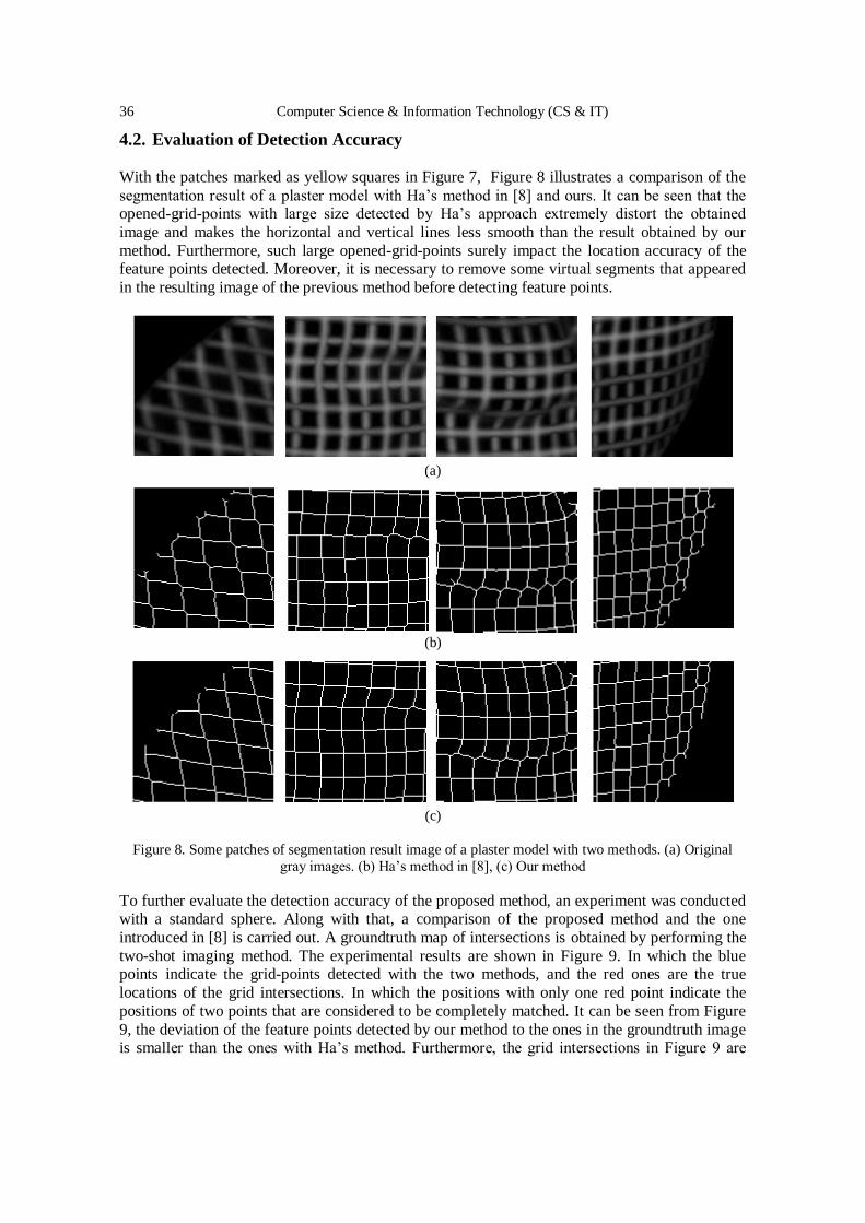
36 Computer Science & Information Technology (CS & IT)
4.2. Evaluation of Detection Accuracy
With the patches marked as yellow squares in Figure 7, Figure 8 illustrates a comparison of the
segmentation result of a plaster model with Ha’s method in [8] and ours. It can be seen that the opened-grid-points with large size detected by Ha’s approach extremely distort the obtained
image and makes the horizontal and vertical lines less smooth than the result obtained by our
method. Furthermore, such large opened-grid-points surely impact the location accuracy of the feature points detected. Moreover, it is necessary to remove some virtual segments that appeared
in the resulting image of the previous method before detecting feature points.
Figure 8. Some patches of segmentation result image of a plaster model with two methods. (a) Original
gray images. (b) Ha’s method in [8], (c) Our method
To further evaluate the detection accuracy of the proposed method, an experiment was conducted with a standard sphere. Along with that, a comparison of the proposed method and the one
introduced in [8] is carried out. A groundtruth map of intersections is obtained by performing the
two-shot imaging method. The experimental results are shown in Figure 9. In which the blue points indicate the grid-points detected with the two methods, and the red ones are the true
locations of the grid intersections. In which the positions with only one red point indicate the
positions of two points that are considered to be completely matched. It can be seen from Figure
9, the deviation of the feature points detected by our method to the ones in the groundtruth image is smaller than the ones with Ha’s method. Furthermore, the grid intersections in Figure 9 are
(a)
(b)
(c)

Computer Science & Information Technology (CS & IT) 37
stretched relatively large so these deviations might be greater than 1 pixel, but they are approximately zero in the quite flat regions.
For a pixel location accuracy of the detected feature points, we define a mean absolute error
(MAE) calculated by the formula (1):
1
| |
,
N
t d
t
C C
MAEN
(1)
Where N denotes the total of detected feature points, Cd is the coordinate of the ones detected in the final image obtained with the two methods, and Ct represents the coordinate of the ones in the
groundtruth image.
It worth noting that, with the feature points are the centers of the opened-grid-points, the pixel
location accuracy of our method is higher than the other proposed in [8] with a MAE value of
0.27 pixels and a maximum error of 2 pixels, while those of Ha’s method are 0.33 and 2 pixels
respectively.
In addition, another index here defined to evaluate the local accuracy of the feature points
detected by the above two methods that calculated by the formula (2):
1 .100%,N
DN
(2)
Where N1 denotes the quantitive of detected feature points with a deviation of less than 1 pixels
to the ones in the groundtruth image, and N indicates the quantitive of all of the detected ones. The experimental results show that this index achieved with our method is 91% which is better
than 78% with Ha’s method.
(a) (b)
Figure 9. Illustration of a pixel location accuracy comparison between the feature points detected with the
method in [8] (a) and the proposed method (b) (marked in blue) and the ones in the
groundtrurth image (marked in red).

38 Computer Science & Information Technology (CS & IT)
Besides the good results obtained during testing and evaluation of the proposed model, our method still has some following limitations:
1) Although using a training set with the labels composed of binary single lines, the model
still produces a grid image with 3 pixels wide stripes, especially for some strongly distorted areas where the stripes’ width might reach 4 pixels. Hence in the final result image, there
still exist some opened-grid-points like Ha's method, however, their size at the
corresponding locations has been significantly reduced.
2) It is quite hard to detect the feature points in a completely new image of a dynamic scene if
there are no images of similar objects acquired with the two-shot imaging method in the training set.
5. CONCLUSIONS
This paper has proposed an approach for detecting the grid-points of the grid pattern for a structured light system mainly based on a U-net network. Along with that, a specific dataset is
designed for training and testing the model. Whereas, the training set includes the patches of
original large gray images and their labeled images, which are captured by utilizing the two-shot imaging method. And the test set consists of grayscale images that are completely different from
the ones in the training set. A comparison between the experimental results obtained with our
method and the two others shows that our method provides better performance. Furthermore, to
evaluate the pixel location accuracy of the feature points detected, an experiment with a standard sphere is conducted. The experimental result proves that the proposed method can achieve a
higher location accuracy comparing with Ha’s in [8]. On the other hand, our method is
convenient to apply to reality applications since it is compatible with both color and monochromatic grid patterns. Moreover, the quality of the point cloud reconstructed can be
improved with such a high performance of feature points detected. To improve the proposed
method, collecting more images of different objects, materials, with different imaging conditions to enrich the training set, and also eliminating the opened-grid-points in the final image for higher
location accuracy of detected feature points is our future scope.
REFERENCES
[1] Joaquim Salvi, Sergio Fernandez, Tomislav Pribanic, and Xavier Llado, (2010) "A state of the art in
structured light patterns for surface profilometry." Pattern Recognition Vol. 43, No. 8, pp 2666-2680.
[2] Xu Zhang, Youfu Li and Limin Zhu, (2012) "Color code identification in coded structured light."
Applied Optics Vol. 51, No. 22, pp 5340-5356.
[3] Yang Lei, Kurt R. Bengtson, Lisa Li, Jan P. Allebach, (2013) "Design and decoding of an M-array
pattern for low-cost structured light 3D reconstruction systems." 2013 IEEE International Conference
on Image Processing, pp 2168-2172.
[4] Tomislav Petković, Tomislav Pribanić and Matea Ðonlić, (2016) "Single-shot dense 3D
reconstruction using self-equalizing De Bruijn sequence." IEEE Transactions on Image Processing Vol. 25, No. 11, pp 5131-5144.
[5] Ali Osman Ulusoy, Fatih Calakli and Gabriel Taubin, (2009) "One-shot scanning using De Bruijn
spaced grids." IEEE 12th International Conference on Computer Vision Workshops, pp 1786-1792.
[6] Guangming Shi, Ruodai Li, Fu Li, Yi Niu and Lili Yang, (2018) "Depth sensing with coding-free
pattern based on topological constraint." Journal of Visual Communication and Image Representation
Vol. 55, 229-242.
[7] Bingyao Huang and Ying Tang, (2014) "Fast 3D reconstruction using one-shot spatial structured
light." 2014 IEEE International Conference on Systems, Man, and Cybernetics, pp 531-536.

Computer Science & Information Technology (CS & IT) 39
[8] Minhtuan Ha, Changyan Xiao, Dieuthuy Pham and Junhui Ge, (2020) "Complete grid pattern
decoding method for a one-shot structured light system." Applied Optics, Vol. 59, No. 9, pp 2674-
2685.
[9] Zhengxin Zhang, Qingjie Liu and Yunhong Wang, (2018) "Road extraction by deep residual u-net."
IEEE Geoscience and Remote Sensing Letters Vol. 15, No. 5, pp 749-753. [10] Chang Wang, Zongya Zhao, Qiongqiong Ren, Yongtao Xu and Yi Yu, (2019) "Dense u-net based on
patch-based learning for retinal vessel segmentation." Entropy Vol. 21, No. 2, pp 168.
[11] Hieu Nguyen, Yuzeng Wang and Zhaoyang Wang, (2020) "Single-Shot 3D Shape Reconstruction
Using Structured Light and Deep Convolutional Neural Networks." Sensors Vol. 20, No. 13, pp 3718.
[12] Suming Tang, Xu Zhang, Zhan Song, Hualie Jiang and Lei Nie, (2017). "Three-dimensional surface
reconstruction via a robust binary shape-coded structured light method." Optical Engineering Vol. 56,
No. 1, 014102.
[13] Zhan Song, Suming Tang, Feifei Gu, Chua Shi and Jianyang Feng, (2019) "DOE-based structured-
light method for accurate 3D sensing." Optics and Lasers in Engineering, Vol. 120, 21-30.
[14] Suming Tang, Xu Zhang, Zhan Song, Lifang Song and Hai Zeng, (2017) "Robust pattern decoding in
shape-coded structured light." Optics and Lasers in Engineering Vol. 96, pp 50-62.
[15] Ryo Furukawa, Daisuke Miyazaki, Masashi Baba, Shinsaku Hiura and Hiroshi Kawasaki (2019), "Robust structured light system against subsurface scattering effects achieved by CNN-based pattern
detection and decoding algorithm." ECCV Workshop 3D Reconstruction in the Wild, pp 372-386.
[16] Dieuthuy Pham, Minhtuan Ha, San Cao and Changyan Xiao, (2020) "Accurate stacked-sheet
counting method based on deep learning." Journal of the Optical Society of America A, Vol. 37, No.
7, pp 1206-1218.
AUTHORS
Minhtuan Ha received the B.S degree in automation from Viet Nam Maritime
University, Hai Phong, Viet Nam, in 2005, and the M.S. degree in Measurement and
Control systems from Ha Noi University of Science and Technology, Ha Noi, Viet
Nam, in 2010. He is currently pursuing a Ph.D. degree with the College of Electrical
and Information Engineering, Hunan University, Changsha, China. His current research
interests include structured light systems, 3D imaging, machine vision and machine
learning.
Dieuthuy Pham received the B.S. degree in automation from Thai Nguyen University,
College of Engineering, Thai Nguyen, Viet Nam, in 2006 and the M.S. degree in Measurement and Control systems from Ha Noi University of Science and Technology,
Ha Noi, Viet Nam, in 2010. She is currently pursuing a Ph.D. degree with the College
of Electrical and Information Engineering, Hunan University, Changsha, China. Her
current research interests include medical image processing, machine vision and
machine learning.
Changyan Xiao received the B.E. and M.S. degrees in mechanical and electronic
engineering from the National University of Defense Technology, Changsha, China, in
1994 and 1997, respectively, and the Ph.D. degree in biomedical engineering from
Shanghai Jiaotong University, Shanghai, China, in 2005., From 2008 to 2009, he was a
Visiting Postdoctoral Researcher with the Division of Image Processing, Leiden University Medical Center, Leiden, Netherlands. Since 2005, he has been an Associate
Professor and a Full Professor with the College of Electrical and Information
Engineering, Hunan University, Changsha. His current research interests include medical imaging and
machine vision. © 2020 By AIRCC Publishing Corporation. This article is published under the Creative Commons
Attribution (CC BY) license.

40 Computer Science & Information Technology (CS & IT)
David C. Wyld et al. (Eds): COMIT, SIPO, AISCA, MLIOB, BDHI - 2020
pp. 41-54, 2020. CS & IT - CSCP 2020 DOI: 10.5121/csit.2020.101604
ARTIST, STYLE AND YEAR CLASSIFICATION
USING FACE RECOGNITION AND CLUSTERING
WITH CONVOLUTIONAL NEURAL NETWORKS
Doruk Pancaroglu
STM A.S., Ankara, Turkey
ABSTRACT Artist, year and style classification of fine-art paintings are generally achieved using standard
image classification methods, image segmentation, or more recently, convolutional neural
networks (CNNs). This works aims to use newly developed face recognition methods such as
FaceNet that use CNNs to cluster fine-art paintings using the extracted faces in the paintings,
which are found abundantly. A dataset consisting of over 80,000 paintings from over 1000
artists is chosen, and three separate face recognition and clustering tasks are performed. The
produced clusters are analyzed by the file names of the paintings and the clusters are named by
their majority artist, year range, and style. The clusters are further analyzed and their performance metrics are calculated. The study shows promising results as the artist, year, and
styles are clustered with an accuracy of 58.8, 63.7, and 81.3 percent, while the clusters have an
average purity of 63.1, 72.4, and 85.9 percent.
KEYWORDS Face Recognition, Clustering, Convolutional Neural Networks, Art Identification
1. INTRODUCTION
Art classification, or more correctly, painting classification in the context of this paper, is a
problem concerned about correctly identifying a piece of art’s creator, the artistic movement it belongs to, and its approximate age. Pieces of art stored in museums are identified and
categorized manually by art experts and curators. As in all things that involve humans, this is a
very error-prone process. There are a lot of cases of art fraud involving museums, auctions, and
large sums of money being paid for worthless reproductions [1].
Art classification by computers is an active area of research because paintings of similar subjects
(still lives, for example) by different painters can have very different styles, leading to varied classification results. A solution to the problem of art classification can also find use in online
museums, educational purposes, and recommendation systems. Currently, most solutions to the
problem of art classification are based on image segmentation [2] or stochastic modeling [3].
Image segmentation is especially useful in classifying modern or abstract art. However, this paper aims to use the methods developed for face recognition to solve the problem of art classification.
Many paintings, excluding the ones with the abstract and modern styles (which will not be featuring in this work obviously), include faces. A large percentage of paintings are portraits, as
they were the bread and butter of painters [4]. A selection of these works can be observed in
Figure 1.

42 Computer Science & Information Technology (CS & IT)
Figure 1: Five paintings from different artists, eras and artistic styles. Note the difference in the styles of
faces, which would prove beneficial in clustering artists, years and styles.
The abundance of faces in the paintings and the fact that many painters have a distinct style of
painting can enable face detection and clustering methods to detect artists from the faces in their paintings. Moreover, the style of faces can also be used to classify the era in which the painting
belongs. The field of image processing has attained great momentum with the introduction of
convolutional neural networks (CNNs). Major social media and technology companies like Google and Facebook have invested in face detection, recognition, and clustering methods that
use CNNs, such as DeepFace [5] and FaceNet [6].
The aim of this paper is to overcome the problem of art classification with face detection and
clustering methods that are using convolutional neural networks (CNNs). The dataset that will be
used in this work is named WikiArt Dataset [7], which contains paintings gathered from WikiArt
[8], a website with a large number of labeled art objects from many different artists and eras.
This paper is organized into six sections. In the first section, the problem is introduced and some
background information is given. In the second section, related work about the problem will be discussed in detail. In the third section, the dataset used in this work will be presented. In the
fourth section, the implementation of the work will be explained. In the fifth section, the results
of the work will be presented. Finally, in the sixth section, the work will be concluded and future directions will be discussed.
2. RELATED WORK
Using computers in the classification of art objects is a relatively new field, but some of the more important achievements will be explained in this section.
Computer Science & Information Technology (CS & IT) 43
Before using CNNs for image processing became popular, two works, the first by S. Lyu, D. Rockmore and H. Farid in 2004 [9], and the second by C. Johnson et al. in 2008 [10], aimed to
identify and authenticate art by analyzing the brush strokes of the paintings. Many famous artists
have distinct brush strokes which are very important to ascertain if the painting in question is a
fake or not. These works use wavelet analysis of the brushstrokes to find out if a painting is an original or a reproduction.
Another work, created by C. Li and T. Chen in 2009 [11] propose a method to evaluate the aesthetic quality of a given piece of art. First, the training set is rated by 23 humans to create a
baseline for aesthetic quality. Then, naïve Bayesian and adaptive boosting (Adaboost [12])
classifiers are used to classify the test set. Finally, the classified images are compared to the human scores and whether a painting is found aesthetic or not is found out.
More recent works that use CNN-backed methods have also appeared. A paper by S. Karayev et
al., published in 2013 [13], used CNN-based stochastic gradient descent classifiers to identify the artistic style of a set of paintings. The results are compared with style labels given to the painting
by humans.
In 2014, authors T. Mensink and J. V. Gemert published a paper [14] consisting of four
challenges accompanied by a dataset of over 110,000 images of pieces of art located in the
Rijksmuseum in Amsterdam, Netherlands. The four challenges were predicting the artist, predicting the type of the art (painting, sculpture, etc.), predicting the material, and lastly,
predicting the year of creation.
The Rijksmuseum Challenge paper proposes baseline experiments for the four challenges as well. These experiments use 1-vs-Rest linear SVM classifiers. The dataset itself has images encoded
with Fisher Vectors [15] that are aggregating local SIFT descriptors, embedded in a global
feature vector.
Another work by L. A. Gatys, A. S. Ecker, and M. Bethge, published in 2015 [16], uses VGG-
Network, a CNN based classifier to create a method that fuses a given photograph with a painting
and creates art. This opens up a different field altogether: can a machine create art?
In 2016, W. R. Tan, C. S. Chan, H. E. Aguirre, and K. Tanaka published a paper [17], in which
paintings are classified using CNNs with respect to their style, genre, and artists. The work had two objectives. Firstly, the work aimed to train a CNN model as a proof-of-concept for art
classification. Secondly, the work aimed to be able to classify modern and abstract art, and tried
to find an answer to the question: “is a machine able to capture imagination?”
One of the motivations for this paper stems from Google Arts & Culture [18]. Created in 2011,
Google Arts & Culture is an online platform functioning as a museum, where partner museums of
Google contribute their collections for online touring. In 2018, an extension to the mobile application of Google Arts & Culture appeared, in which the user’s selfie would be matched with
a portrait stored in the databases of Google Arts & Culture. For this, Google uses its own CNN
face recognition method, FaceNet, which will be explained in detail in the following paragraph.
FaceNet is a face recognition method developed by researchers from Google, F. Schroff, D.
Kalenichenko, and J. Philbin in 2015 [6]. FaceNet uses deep convolutional networks that are trained for direct optimization for embedding, which itself is the process of measuring the facial
similarities between two images.
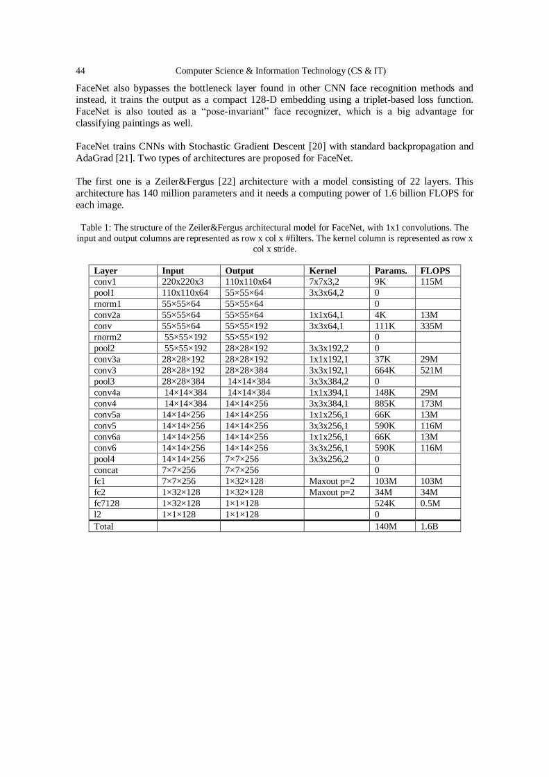
44 Computer Science & Information Technology (CS & IT)
FaceNet also bypasses the bottleneck layer found in other CNN face recognition methods and instead, it trains the output as a compact 128-D embedding using a triplet-based loss function.
FaceNet is also touted as a “pose-invariant” face recognizer, which is a big advantage for
classifying paintings as well.
FaceNet trains CNNs with Stochastic Gradient Descent [20] with standard backpropagation and
AdaGrad [21]. Two types of architectures are proposed for FaceNet.
The first one is a Zeiler&Fergus [22] architecture with a model consisting of 22 layers. This
architecture has 140 million parameters and it needs a computing power of 1.6 billion FLOPS for
each image.
Table 1: The structure of the Zeiler&Fergus architectural model for FaceNet, with 1x1 convolutions. The
input and output columns are represented as row x col x #filters. The kernel column is represented as row x
col x stride.
Layer Input Output Kernel Params. FLOPS
conv1 220x220x3 110x110x64 7x7x3,2 9K 115M
pool1 110x110x64 55×55×64 3x3x64,2 0
rnorm1 55×55×64 55×55×64 0
conv2a 55×55×64 55×55×64 1x1x64,1 4K 13M
conv 55×55×64 55×55×192 3x3x64,1 111K 335M
rnorm2 55×55×192 55×55×192 0
pool2 55×55×192 28×28×192 3x3x192,2 0
conv3a 28×28×192 28×28×192 1x1x192,1 37K 29M
conv3 28×28×192 28×28×384 3x3x192,1 664K 521M
pool3 28×28×384 14×14×384 3x3x384,2 0
conv4a 14×14×384 14×14×384 1x1x394,1 148K 29M
conv4 14×14×384 14×14×256 3x3x384,1 885K 173M
conv5a 14×14×256 14×14×256 1x1x256,1 66K 13M
conv5 14×14×256 14×14×256 3x3x256,1 590K 116M
conv6a 14×14×256 14×14×256 1x1x256,1 66K 13M
conv6 14×14×256 14×14×256 3x3x256,1 590K 116M
pool4 14×14×256 7×7×256 3x3x256,2 0
concat 7×7×256 7×7×256 0
fc1 7×7×256 1×32×128 Maxout p=2 103M 103M
fc2 1×32×128 1×32×128 Maxout p=2 34M 34M
fc7128 1×32×128 1×1×128 524K 0.5M
l2 1×1×128 1×1×128 0
Total 140M 1.6B

Computer Science & Information Technology (CS & IT) 45
Table 2: The structure of the inception architectural model for FaceNet
Type Output
Size
Depth #1x1 #3x3
reduce
#3x3 #5x5
redu
ce
#5x5 Pool
proj
(p)
Para
ms.
FLOPS
conv1 (7x7x3,2)
112x112x64 1 9K 119M
max pool + norm
56x56x64 0 m 3x3,2
inception (2)
56x56x192 2 64 192 115K 360M
norm + max pool
28x28x192 0 m 3x3,2
inception (3a)
28x28x256 2 64 96 128 16 32 m, 32p
164K 128M
inception
(3b)
28x28x320 2 64 96 128 32 64 L2,
64p
228K 179M
inception (3c)
14x14x640 2 0 128 256,2 32 64,2 m 3x3,2
398K 108M
inception (4a)
14x14x640 2 256 96 192 32 64 L2, 128p
545K 107M
inception
(4b)
14x14x640 2 224 112 224 32 64 L2,
128p
595K 117M
inception (4c)
14x14x640 2 192 128 256 32 64 L2, 128p
654K 128M
inception (4d)
14x14x640 2 160 144 288 32 64 L2, 128p
722K 142M
inception
(4e)
7x7x1024 2 0 160 256,2 64 128,2 m
3x3,2
717K 56M
inception (5a)
7x7x1024 2 384 192 384 48 128 L2, 128p
1.6M 78M
inception (5b)
7x7x1024 2 384 192 384 48 128 m, 128p
1.6M 78M
avg pool 1x1x1024 0
fully conn 1x1x128 1 131K 0.1M
L2 normalizatio
n
1x1x128 0
Total 7.5M 1.6B
The second architecture is based on the GoogleNet style Inception Models [23]. This architecture
is 17 layers deep. This architecture is composed of 7,5 million parameters and it consumes less computing power compared to the first one.
Detailed information about these two architectures can be found in Tables 1 and 2.
FaceNet achieved high results, even higher than humans in well-known facial recognition
benchmarks such as Labelled Faces in the Wild (LFW) [24] and Youtube Faces Database (YDB)
[25]. These results can be seen in Table 3.

46 Computer Science & Information Technology (CS & IT)
Table 3: The accuracy values of FaceNet and other prominent face recognition methods tested with the
datasets LFW and YDB. The values denoted in bold are the highest scores.
Method Accuracy
(LFW)
Accuracy
(YDB)
FaceNet 0.9963 0.9512
Humans 0.9920 -
DeepFace 0.9735 0.9140
Joint Bayesian [26] 0.9633 -
DDML[27] 0.9068 0.8230
LM3L [28] 0.8957 0.8130
Eigen-PEP [29] 0.8897 0.8480
CNN-3DMM [30] 0.8880 0.9235
APEM (fusion) [31] 0.8408 0.7910
There are several code implementations of FaceNet available on GitHub. The one created by David Sandberg [35] is selected for its ease of use and better documentation.
3. DATASET The dataset used in this work is named WikiArt Dataset. The dataset is created for the paper
published by B. Saleh and A. Elgammal in 2015 [32]. The work itself is an SVM-based art
classification method.
The dataset is created with the paintings collected from the WikiArt website. WikiArt is arguably
the largest online and free collection of digitized paintings.
The dataset contains 81,479 paintings from 2,148 artists. The paintings are also categorized into
styles from different periods of art history, totaling 27. Lastly, paintings are categorized into 45
genres such as still lives or portraits.
In the work by B. Saleh and A. Elgammal, The dataset is grouped into three different subsets for
three distinct classifications challenges: style identification, genre identification, and artist
identification.
For the style identification challenge, the dataset is subdivided into 27 styles with at least 1,500
paintings each, with a total of 78,449 paintings. For the genre identification challenge, the dataset is subdivided into 10 genres with at least 1,500 paintings each, totaling 63,691 paintings.
For the artist identification challenge, the dataset is subdivided into 23 artists with at least 500
paintings each, with a total of 18,599 paintings.
The detailed styles, genres, and artists (25 of the 1,119) groupings of the WikiArt dataset can be
seen in Table 4.
For this paper, the styles that do not have any faces (action paintings, abstract expressionism) or a
majority of faces in their paintings (color field painting, pop-art), or with faces that are not suitable for recognition (cubism) are removed from the dataset. This reduces the total number of
paintings in the dataset to 67,064, with 16 styles and 1,382 artists.

Computer Science & Information Technology (CS & IT) 47
Table 4: List of styles, genres (not used in the scope of this work) and an incomplete list of painters present
in the WikiArt dataset. The styles marked with (*) are omitted from this work because of the lack of faces or the faces being distorted.
Classification
Task
List of Members
Style Abstract Expressionism(*); Action Painting(*); Analytical Cubism(*); Art
Nouveau Modern Art; Baroque; Color Field Painting(*); Contemporary
Realism; Cubism(*); Early Renaissance; Expressionism; Fauvism(*); High
Renaissance; Impressionism; Mannerism-Late-Renaissance; Minimalism(*);
Primitivism-Naive Art(*); New Realism; Northern Renaissance; Pointillism;
Pop Art(*); Post Impressionism; Realism; Rococo; Romanticism; Symbolism;
Synthetic Cubism(*); Ukiyo-e(*)
Genre Abstract painting; Cityscape; Genre painting; Illustration; Landscape; Nude painting; Portrait; Religious painting; Sketch and Study; Still Life
Artist (Selected) Leonardo Da Vinci, Michelangelo, Caravaggio, Diego Velazquez, El Greco;
Albrecht Durer; Francisco Goya; Boris Kustodiev; Camille Pissarro; Claude
Monet; Edgar Degas; Eugene Boudin; Gustave Dore; Ilya Repin; Ivan
Aivazovsky; Ivan Shishkin; John Singer Sargent; Marc Chagall; Nicholas
Roerich; Pablo Picasso; Paul Cezanne; Pierre-Auguste Renoir; Rembrandt;
Salvador Dali; Vincent van Gogh
4. IMPLEMENTATION As mentioned in section 2, David Sandberg’s FaceNet implementation is selected to run
FaceNet’s face clustering method with WikiArt dataset. This implementation works with
Tensorflow [33], an open-source machine learning framework with CUDA support. The implementation is written using Python.
For computational purposes, paintings from the following styles are selected with all their available artists: Early Renaissance, High Renaissance, Late Renaissance, Northern Renaissance,
Baroque and Rococo. These 6 styles amount to 12,907 paintings and 192 artists.
4.1. Pre-processing
Firstly the preprocessing phase is done. This phase is called the alignment phase in the
implementation, meaning that only the face and a given margin is extracted from a larger image. A sample process can be seen in Figure 2.
In our case, the face or if present, multiple faces are extracted from the paintings. Extracting multiple faces from a painting provides better insight into an artist’s style of painting a face.
In the alignment phase, the output image size is selected as 160x160 pixels and the margin for the
area around the bounding box of the face is 32 pixels.
4.2. Training Secondly, the training phase begins. For this phase, the training model is obtained by training the
classifier on the VGGFace2 dataset [34] created by Q. Cao, L. Shen W. Xie, O. M. Parkhi, and A.
Zisserman. This dataset contains 3.3 million images for over 9,000 people.

48 Computer Science & Information Technology (CS & IT)
Figure 2: The results of the face extraction process used in three different paintings. The extraction process
also works for multiple faces in the paintings.
4.3. Clustering
For the clustering operation itself, DBSCAN [34] algorithm, created by J. Sander, M. Ester, H. P.
Kriegel, and X. Xu, is used. The minimum number of required images to form a cluster set at 25. The clustering operation runs the FaceNet face recognition method and clusters the similar faces,
based on the Euclidean distance matrix.
4.3. Analyzing
Following the clustering operation, the produced clusters are analyzed using the file names of the paintings in the clusters. The file names contain the artist’s name, the name of the painting, the
style of the painting, and the year of completion (it should be noted that in the dataset, not all
paintings have a year of completion).
After the file names are parsed, the second part of the analyzing phase starts. In this phase, the
clusters are named according to the dominant artist, style, or year. If no dominant artist, style, or
year is found in a cluster, that cluster is omitted from the results.
To achieve a better image classification accuracy in terms of years, the years of the paintings are
grouped in 50-year periods (e.g., if a cluster has a majority of paintings dated from years 1500 to 1550, that cluster is named 1500-1550).
5. RESULTS AND EVALUATION
In the evaluation of this work, all the clusters are evaluated three times for the three tasks of classification: artist classification, style classification, and year classification.
Four different values make up the formulas of the results: True Positive (TP), False Positive (FP), True Negative (TN), and False Negative (FN).

Computer Science & Information Technology (CS & IT) 49
In the context of this work and the produced clusters, TP is the total number of paintings that are present in their correct clusters (i.e. the paintings belonging to the majority artist of a cluster). FP
is the total number of paintings that are present in the cluster, but not belonging to the majority
artist of that cluster. TN is the total number of paintings that are not present in the cluster, and
also not belonging to the majority artist of the cluster. FN is the total number of paintings that are not present in the cluster, but belonging to the majority artist of that cluster. The results are
separated into two groups, cluster-specific and inter-cluster.
5.1. Cluster-Specific Results
Four different metrics are calculated for each cluster. The metrics in question are accuracy, precision, recall, and f-measure. The accuracy metric is the general rate of the correctness of the
cluster’s artist compared to the whole dataset. As this metric does not give a meaningful
explanation of the results by itself, other metrics are also used.
The metric of precision is the rate of the correctness the cluster’s artist in a given cluster, while
recall is the rate of the correctness of that cluster’s artist in the whole dataset. F-measure, or F1 score, is a measure that combines precision and recall, the harmonic mean of the two.
The formulas can be observed in Equations (1), (2), (3), and (4).
𝐴𝑐𝑐𝑢𝑟𝑎𝑐𝑦 =𝑇𝑃+𝑇𝑁
𝑇𝑃+𝑇𝑁+𝐹𝑃+𝐹𝑁
𝑃𝑟𝑒𝑐𝑖𝑠𝑖𝑜𝑛 =𝑇𝑃
𝑇𝑃+𝐹𝑁
𝑅𝑒𝑐𝑎𝑙𝑙 =𝑇𝑃
𝑇𝑃+𝐹𝑃
𝐹 − 𝑀𝑒𝑎𝑠𝑢𝑟𝑒 = 2 ×𝑃𝑟𝑒𝑐𝑖𝑠𝑖𝑜𝑛×𝑅𝑒𝑐𝑎𝑙𝑙
𝑃𝑟𝑒𝑐𝑖𝑠𝑖𝑜𝑛+𝑅𝑒𝑐𝑎𝑙𝑙
A selection of the results of the formed clusters which have a majority, separated by their tasks
can be observed in Tables 5, 6, and 7. Considering the large number of artists, styles, and year
periods in the dataset, not all clusters produced in the classification tasks are present in these tables.
5.2. Inter-Cluster Results
In addition to the cluster-specific results, metrics concerning all the created clusters are
calculated. These metrics are purity, normalized mutual information (NMI), and Rand Index (RI).
Purity is a straightforward measure, similar to accuracy that produces a general quality of
clustering. But for clusters with single items, purity tends to produce misleading results. The problem is solved by using normalized mutual information. NMI is useful at producing
normalized values for evaluating the quality of clustering.
The final metric, Rand Index is a measure of similarity between clusters. RI is calculated by
adding the pairs of total TP and TN values in every cluster and dividing this value by the total
number of images.
These formulas can be observed in Equations (5), (6), and (7).
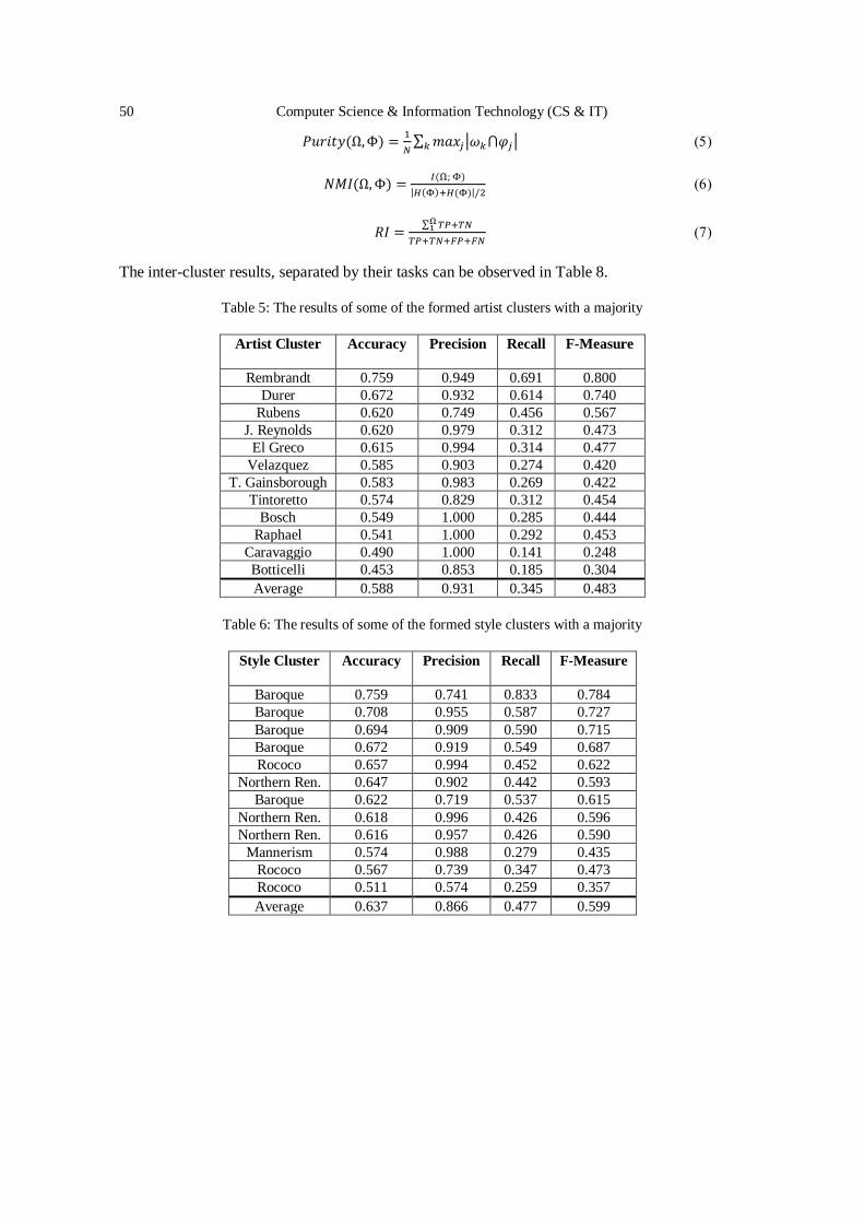
50 Computer Science & Information Technology (CS & IT)
𝑃𝑢𝑟𝑖𝑡𝑦(Ω, Φ) =1
𝑁∑ 𝑚𝑎𝑥𝑗|𝜔𝑘⋂𝜑𝑗|𝑘
𝑁𝑀𝐼(Ω, Φ) =𝐼(Ω; Φ)
|𝐻(Φ)+𝐻(Φ)|/2
𝑅𝐼 =∑ 𝑇𝑃+𝑇𝑁Ω
1
𝑇𝑃+𝑇𝑁+𝐹𝑃+𝐹𝑁
The inter-cluster results, separated by their tasks can be observed in Table 8.
Table 5: The results of some of the formed artist clusters with a majority
Artist Cluster Accuracy Precision Recall F-Measure
Rembrandt 0.759 0.949 0.691 0.800
Durer 0.672 0.932 0.614 0.740
Rubens 0.620 0.749 0.456 0.567
J. Reynolds 0.620 0.979 0.312 0.473
El Greco 0.615 0.994 0.314 0.477
Velazquez 0.585 0.903 0.274 0.420
T. Gainsborough 0.583 0.983 0.269 0.422
Tintoretto 0.574 0.829 0.312 0.454
Bosch 0.549 1.000 0.285 0.444
Raphael 0.541 1.000 0.292 0.453
Caravaggio 0.490 1.000 0.141 0.248
Botticelli 0.453 0.853 0.185 0.304
Average 0.588 0.931 0.345 0.483
Table 6: The results of some of the formed style clusters with a majority
Style Cluster Accuracy Precision Recall F-Measure
Baroque 0.759 0.741 0.833 0.784
Baroque 0.708 0.955 0.587 0.727
Baroque 0.694 0.909 0.590 0.715
Baroque 0.672 0.919 0.549 0.687
Rococo 0.657 0.994 0.452 0.622
Northern Ren. 0.647 0.902 0.442 0.593
Baroque 0.622 0.719 0.537 0.615
Northern Ren. 0.618 0.996 0.426 0.596
Northern Ren. 0.616 0.957 0.426 0.590
Mannerism 0.574 0.988 0.279 0.435
Rococo 0.567 0.739 0.347 0.473
Rococo 0.511 0.574 0.259 0.357
Average 0.637 0.866 0.477 0.599

Computer Science & Information Technology (CS & IT) 51
Table 7: The results of some of the formed clusters with a majority
Year Cluster Accuracy Precision Recall F-Measure
1600-1650 0.904 0.996 0.899 0.945
1650-1700 0.858 0.950 0.860 0.903
1600-1650 0.856 0.964 0.867 0.913
1600-1650 0.856 0.969 0.865 0.914
1700-1750 0.820 0.998 0.767 0.867
1700-1750 0.816 0.989 0.757 0.857
1600-1650 0.815 0.904 0.867 0.885
1600-1650 0.812 0.901 0.863 0.882
1650-1700 0.809 0.978 0.792 0.875
1550-1600 0.802 0.953 0.789 0.863
1500-1550 0.766 0.895 0.798 0.844
1500-1550 0.649 0.756 0.754 0.755
Average 0.813 0.938 0.823 0.875
Table 8: The results of the cluster groups produced by their tasks. Note that the number of style
and year clusters are much higher than the number of distinct styles and year-periods of the dataset. Thus, different clusters are treated as one when calculating accuracy.
Cluster # of Clusters Accuracy Purity NMI RI
Artist 115 0.598 0.631 0.394 0.489
Style 86 0.666 0.724 0.407 0.563
Year 30 0.875 0.859 0.440 0.645
Average - 0.712 0.738 0.413 0.565
5.3. Evaluation
The results will be explained and evaluated according to the three classification tasks.
The artist classification task produced 126 clusters. 115 of these clusters had a majority artist.
These clusters produced an average accuracy, precision, recall, and f-measure values of 58.8%, 93.1%, 34.5%, and 48.3% respectively. The artist clusters, on the whole, are created with the
purity, NMI and RI values of 63.1%, 39.4%, and 48.9% respectively.
The results of the artist classification clusters were not strictly high. This can be attributed to the selected styles which include a lot of religious paintings. This caused one of the clusters to have a
majority of Jesus Christ faces painted by different artists.
It can also be seen that artists from the early renaissance were harder to cluster while later periods
such as baroque and rococo produced clusters with more defined artists and higher metrics.
Nevertheless, clusters of artists with a distinct style such as Rembrandt, Dürer, and El Greco have
relatively higher scores.
In terms of style, 88 clusters in total were created, with 86 of them having a majority of paintings
belonging to the same artistic style. These clusters produced an average accuracy, precision, recall, and f-measure values of 63.7%, 86.6%, 47.7%, and 59.9% respectively. The style clusters,
on the whole, are created with the purity, NMI and RI values of 72.4%, 40.7%, and 56.3%
respectively.

52 Computer Science & Information Technology (CS & IT)
An interesting case in this is that while only 6 different styles from the dataset were used for clustering, numerous different clusters would have a majority of the same style. This can be
attributed to the fact that the dataset is composed of paintings produced roughly between the
years 1400 and 1750, and a large part of that year interval has paintings that are more or less
similar in style. The true difference in artistic styles started to occur in the 19th century.
In terms of years, 74 clusters in total were created, with 30 of them having a majority. The large
difference between the created clusters and the ones with majorities is because the need for a majority of 50-year periods is lacking in most of them. These clusters produced an average
accuracy, precision, recall, and f-measure values of 81.3%, 93.8%, 82.3%, and 87.5%
respectively. The style clusters, on the whole, are created with the purity, NMI, and RI values of 87.5%, 44.0%, and 64.5% respectively.
Similar, but not as abundant as the style clusters, year clusters also had multiple majorities that
pointed to the same 50-year periods. This can be attributed to the difference in parameters used in the artist clustering and the style and year clustering tasks.
It should be noted that using the same parameters (especially higher threshold) for both tasks did not necessarily lead to a lower number of clusters, which would ideally be 6 for styles and 10 for
50-year periods. It can be surmised that for a more accurate year and style classifications, more
refined methods are needed.
6. CONCLUSION
It can be said that classifying fine-art paintings by extracting the faces in them, and running face
detection methods with CNNs is a novel and promising approach.
While artist classification performance is lower than style and year classification performances,
this is understandable considering the explanations given in the evaluation part of chapter 5.
Not withholding the fact that this approach works only with paintings that include a face or faces, and thus it is unable to be of any use for the works of many great artists who do not paint faces,
this type of approach would still be useful in a variety of situations such as art recommendation
and educational purposes.
Future directions of this work include using the whole WikiArt dataset for more refined results,
using other prominent art datasets, and implementing different face recognition and clustering methods to compare their performances. Combining this approach with other art classification
solutions (analyzing brush strokes, for example) would solve some of the shortcomings of the
work, such as the similar art styles of the earlier eras. Finally, creating bigger clusters for style
and year classification tasks is another future objective.
REFERENCES [1] Subramanian, S. (2018, June 15). How to spot a perfect fake: The world's top art forgery detective.
Retrieved from https://www.theguardian.com/news/2018/jun/15/how-to-spot-a-perfect-fake-the-
worlds-top-art-forgery-detective
[2] Haladova, Z. (2010, May). Segmentation and classification of fine art paintings. In 14th Central
European Seminar on Computer Graphics (p. 59).
[3] Shen, J. (2009). Stochastic modeling western paintings for effective classification. Pattern
Recognition, 42(2), 293-301.

Computer Science & Information Technology (CS & IT) 53
[4] Portrait of the artist as an entrepreneur. (2011, December 17). Retrieved from
https://www.economist.com/christmas-specials/2011/12/17/portrait-of-the-artist-as-an-entrepreneur
[5] Taigman, Y., Yang, M., Ranzato, M. A., & Wolf, L. (2014). Deepface: Closing the gap to human-
level performance in face verification. In Proceedings of the IEEE conference on computer vision and
pattern recognition (pp. 1701-1708). [6] Schroff, F., Kalenichenko, D., & Philbin, J. (2015). Facenet: A unified embedding for face
recognition and clustering. In Proceedings of the IEEE conference on computer vision and pattern
recognition (pp. 815-823).
[7] https://github.com/cs-chan/Artwork-Synthesis/tree/master/WikiArt%20Dataset
[8] https://www.wikiart.org/
[9] Lyu, S., Rockmore, D., & Farid, H. (2004). A digital technique for art authentication. Proceedings of
the National Academy of Sciences of the United States of America, 101(49), 17006-17010.
[10] Johnson, C. R., Hendriks, E., Berezhnoy, I. J., Brevdo, E., Hughes, S. M., Daubechies, I., ... & Wang,
J. Z. (2008). Image processing for artist identification. IEEE Signal Processing Magazine, 25(4).
[11] Li, C., & Chen, T. (2009). Aesthetic visual quality assessment of paintings. IEEE Journal of selected
topics in Signal Processing, 3(2), 236-252.
[12] Freund, Y., & Schapire, R. E. (1997). A decision-theoretic generalization of on-line learning and an application to boosting. Journal of computer and system sciences, 55(1), 119-139.
[13] Karayev, S., Trentacoste, M., Han, H., Agarwala, A., Darrell, T., Hertzmann, A., & Winnemoeller, H.
(2013). Recognizing image style. arXiv preprint arXiv:1311.3715.
[14] Mensink, T., & Van Gemert, J. (2014, April). The rijksmuseum challenge: Museum-centered visual
recognition. In Proceedings of International Conference on Multimedia Retrieval (p. 451). ACM.
[15] Sánchez, J., Perronnin, F., Mensink, T., & Verbeek, J. (2013). Image classification with the fisher
vector: Theory and practice. International journal of computer vision, 105(3), 222-245.
[16] Gatys, L. A., Ecker, A. S., & Bethge, M. (2015). A neural algorithm of artistic style. arXiv preprint
arXiv:1508.06576.
[17] Tan, W. R., Chan, C. S., Aguirre, H. E., & Tanaka, K. (2016, September). Ceci n'est pas une pipe: A
deep convolutional network for fine-art paintings classification. In Image Processing (ICIP), 2016 IEEE International Conference on (pp. 3703-3707). IEEE.
[18] https://artsandculture.google.com/
[19] LeCun, Y., Boser, B., Denker, J. S., Henderson, D., Howard, R. E., Hubbard, W., & Jackel, L. D.
(1989). Backpropagation applied to handwritten zip code recognition. Neural computation, 1(4), 541-
551.
[20] Duchi, J., Hazan, E., & Singer, Y. (2011). Adaptive subgradient methods for online learning and
stochastic optimization. Journal of Machine Learning Research, 12(Jul), 2121-2159.
[21] Zeiler, M. D., & Fergus, R. (2014, September). Visualizing and understanding convolutional
networks. In European conference on computer vision (pp. 818-833). Springer, Cham.
[22] Szegedy, C., Liu, W., Jia, Y., Sermanet, P., Reed, S., Anguelov, D., ... & Rabinovich, A. (2015).
Going deeper with convolutions. In Proceedings of the IEEE conference on computer vision and
pattern recognition (pp. 1-9). [23] http://vis-www.cs.umass.edu/lfw/
[24] https://www.cs.tau.ac.il/~wolf/ytfaces/
[25] Chen, D., Cao, X., Wang, L., Wen, F., & Sun, J. (2012, October). Bayesian face revisited: A joint
formulation. In European Conference on Computer Vision (pp. 566-579). Springer, Berlin,
Heidelberg.
[26] Hu, J., Lu, J., & Tan, Y. P. (2014). Discriminative deep metric learning for face verification in the
wild. In Proceedings of the IEEE Conference on Computer Vision and Pattern Recognition (pp. 1875-
1882).
[27] Hu, J., Lu, J., Yuan, J., & Tan, Y. P. (2014, November). Large margin multi-metric learning for face
and kinship verification in the wild. In Asian Conference on Computer Vision (pp. 252-267).
Springer, Cham. [28] Li, H., Hua, G., Shen, X., Lin, Z., & Brandt, J. (2014, November). Eigen-pep for video face
recognition. In Asian Conference on Computer Vision (pp. 17-33). Springer, Cham.
[29] Tran, A. T., Hassner, T., Masi, I., & Medioni, G. (2017, July). Regressing robust and discriminative
3D morphable models with a very deep neural network. In Computer Vision and Pattern Recognition
(CVPR), 2017 IEEE Conference on (pp. 1493-1502). IEEE.

54 Computer Science & Information Technology (CS & IT)
[30] Li, H., Hua, G., Lin, Z., Brandt, J., & Yang, J. (2013). Probabilistic elastic matching for pose variant
face verification. In Proceedings of the IEEE Conference on Computer Vision and Pattern
Recognition (pp. 3499-3506).
[31] Saleh, B., & Elgammal, A. (2015). Large-scale classification of fine-art paintings: Learning the right
metric on the right feature. arXiv preprint arXiv:1505.00855. [32] https://www.tensorflow.org/
[33] https://www.robots.ox.ac.uk/%7Evgg/data/vgg_face2/
[34] Sander, J., Ester, M., Kriegel, H. P., & Xu, X. (1998). Density-based clustering in spatial databases:
The algorithm gdbscan and its applications. Data mining and knowledge discovery, 2(2), 169-194.
[35] https://github.com/davidsandberg/facenet
AUTHORS
Doruk Pancaroglu has been working at STM A.S. as a senior software engineer since
2012. He is a PhD student of computer engineering at Hacettepe University since 2016.
He obtained his BSc for Computer Engineering from Sabanci University in 2010 and his
MSc for Computer Engineering from TOBB ETU in 2014. Since 2012, he has been
working at STM A.S. as a senior software engineer. His research interests are network
security, internet of things and machine learning, with a focus on IoT security.
© 2020 By AIRCC Publishing Corporation. This article is published under the Creative Commons
Attribution (CC BY) license.

David C. Wyld et al. (Eds): COMIT, SIPO, AISCA, MLIOB, BDHI - 2020
pp. 55-64, 2020. CS & IT - CSCP 2020 DOI: 10.5121/csit.2020.101605
MULTI SCALE TEMPORAL GRAPH
NETWORKS FOR SKELETON-BASED ACTION RECOGNITION
Tingwei Li1, Ruiwen Zhang2, Qing Li1
1Department of Automation Tsinghua University, Beijing, China
2Department of Computer Science Tsinghua University, Beijing, China
ABSTRACT Graph convolutional networks (GCNs) can effectively capture the features of related nodes and
improve the performance of model. More attention is paid to employing GCN in Skeleton-Based
action recognition. But existing methods based on GCNs have two problems. First, the
consistency of temporal and spatial features is ignored for extracting features node by node and
frame by frame. To obtain spatiotemporal features simultaneously, we design a generic
representation of skeleton sequences for action recognition and propose a novel model called
Temporal Graph Networks (TGN). Secondly, the adjacency matrix of graph describing the
relation of joints are mostly depended on the physical connection between joints. To
appropriate describe the relations between joints in skeleton graph, we propose a multi-scale
graph strategy, adopting a full-scale graph, part-scale graph and core-scale graph to capture
the local features of each joint and the contour features of important joints. Experiments were
carried out on two large datasets and results show that TGN with our graph strategy
outperforms state-of-the-art methods.
KEYWORDS Skeleton-based action recognition, Graph convolutional network, Multi-scale graphs.
1. INTRODUCTION
Human action recognition is a meaningful and challenging task. It has widespread potential
applications, including health care, human-computer interaction and autonomous driving. At
present, skeleton data is more often used for action recognition because skeleton data is robust to
the noise of background and different viewpoints compared to video data. Skeleton-based action
recognition are mainly based on deep learning methods like Recurrent Neural Networks (RNNs),
Convolutional Neural Networks (CNNs) and GCNs [3, 8, 10, 12, 13, 15, 17, 18,]. RNNs and
CNNs generally process the skeleton data into vector sequence and image respectively. These
representing methods cannot fully express the dependencies between correlated joints. With more
researches on GCN, [12] first employs GCN in skeleton-based action recognition and inspires a
lot of new researches [7, 10, 15, 17, 18].
The key of action recognition based on GCN is to obtain the temporal and spatial features of an
action sequence through graph [7, 10, 18]. In the skeleton graph, skeleton joints transfer into node
and the relations between joints are represented by edges. As shown in Fig. 1, in most previous
work, there are more than one graphs, a node only contains spatial features. In this case, GCN
extracts spatial features frame by frame, then Temporal Convolutional Network (TCN) extracts

56 Computer Science & Information Technology (CS & IT)
temporal features node by node. But, features of a joint in an action is not only related to other
joints intra frames but also joints inter frames. As a result, existing methods split this consistency
of spatiotemporal features. To solve this problem, we propose TGN to capture spatiotemporal
features simultaneously, as shown in Fig. 2, each node composes a joint of all frames and
contains both spatial and temporal feature in the graph, thus TGN obtains spatiotemporal features
by processing all frames of each joint simultaneously.
Besides, the edges of skeleton graph mainly depend on the adjacency matrix A, which is related
to the physical connections of joints [12,17,18]. GCN still have no effective adaptive graph
mechanism to establish a global connection through the physical relations of nodes, such as a
relation between head and toes. GCN can only obtain local features, such as a relation between
head and neck. In this paper, a multi-scale graph strategy is proposed, which adopts different
scale graphs in different network branches, as a result, physically unconnected information is
added to help network capture the local features of each joint and the contour features of
important joints.
The major contributions of this work lie in three aspects:
(1) This paper proposes a feature extractor called Temporal Graph Network (TGN) to obtain
spatiotemporal features simultaneously, and this extractor can be fitted in and perform
better than most skeleton-based action recognition models based on GCN.
(2) We devisea multi-scale graph strategy for optimization of graph to capture both the local
features and the contour features.
(3) Combining the multi-scale graph strategy with TGN, we propose Multi-scale Temporal
Graph Network (MS-TGN) which outperforms state-of-the-art methods on two large
scale datasets for skeleton-based action recognition.
2. RELATED WORKS
2.1. Action Recognition based on Skeleton
The methods of skeleton-based action recognition can be classified into two kinds, using
handcrafted features to model human bodies and using deep learning methods respectively. Using
handcrafted features [5, 14] are quite complex and more suitable for small and medium-sized
datasets. Deep learning methods are based on three models, RNNs, CNNs and GCNs. RNN-
based methods [3, 19, 22] model temporal dependencies over sequences from skeletons. CNN-
based approaches [2, 8] usually transfer the skeleton data as an image. For these methods cannot
express a meaningful operator in the vertex domain. Recently, researchers tend to GCN [10, 12,
15, 18] and build operators in the non-Euclidean space.
2.2. Graph Convolutional Networks
In action recognition task, the principle of constructing GCN on the graph generally follows the
spatial perspective [1], where the convolutional filters are applied directly to the graph nodes.
Several classic methods in this task are proposed in recent two years. [12] embeds skeleton
sequences into several graphs where joints in a frame of a sequence make up nodes of a graph
and relations between joints are spatial edges of a graph. [18] gives a two-stream GCN
architecture, which takes the second-order information (bones) into consideration and employs
graph adaptiveness to optimize the adjacent matrix. [17] proposes graph regression based on
GCN to exploit the dependencies of each joints. [15] employs Neural Architecture Search (NAS)
to existing model to automatically design GCN.

Computer Science & Information Technology (CS & IT) 57
3. OUR METHODS
3.1. Temporal Graph Networks
The skeleton data of an action can be described as 𝑋 = {𝑥𝑐,𝑣,𝑡}𝐶×𝑉×𝑇
, where 𝑇 is the number
offrames, 𝑉 is number of joints in a frame, 𝐶 is number of channels in a joint and 𝑥𝑐,𝑣,𝑡 represents
the skeleton data of joint 𝑣 in the frame t with 𝑐 channels .𝑋𝑖 is the sequence 𝑖. Previous methods
construct 𝑇 graphs and each graph has𝑉 nodes, as shown in Fig. 1, where the node set 𝑁 =
{𝑥 𝑣,𝑡|, 𝑣 = 1,2, … 𝑉, 𝑡 = 1,2 … 𝑇}𝐶
has joint 𝑣 in 𝑡𝑡ℎ frame. It means a frame is represented as one
graph and there are totally 𝑇 graphs. The size feature of a node is 𝐶. GCN is used to obtain spatial
features from each graph, then outputs of GCN are fed into TCN to extract temporal features.
Figure 1. A node in any graph represents data of a joint in a certain frame. GCN extracts spatial features
frame by frame, and TCN extracts temporal features node by node.
We redefine graph and propose TGN. Compared to 𝑇 graphs, we only have one graph with 𝑉
nodes, as seen in Fig. 2. In the graph, the node set 𝑁 = {𝑥𝑣|𝑣 = 1,2 … 𝑇}𝐶×𝑉 has the joint 𝑣 in all
frame. The size of feature of a node is 𝐶 × 𝑉. Compared with series methods using GCN and
TCN alternately, we only use one GCN block to realize the extraction of spatiotemporal features.
Figure 2. Each node represents data of a joint in all frames so temporal information is also contained.
Compared with Fig1, TGN extracts temporal and spatial features simultaneously.
In a basic TGN block, each node already has temporal information and spatial information,
therefore, in the process of graph convolution, temporal and spatial features can be calculated
simultaneously. The output value for a single channel at the spatial location 𝑁𝑣 can be written as
Eq. 2.
𝑆𝑣 = {𝑛𝑗|𝑛𝑗 ∈ 𝑆(𝑁𝑣, ℎ)} (1)

58 Computer Science & Information Technology (CS & IT)
𝐹𝑜(𝑁𝑣) = ∑(𝐹𝑖(𝑆𝑣(𝑗)) × 𝑤(𝑗)
𝑘
𝑗=0
) (2)
Where 𝑁𝑣is node 𝑣. 𝑠(𝑁𝑣 , ℎ)is a sampling function used to find node set 𝑛𝑗 adjacent to the node𝑁𝑣,
𝐹𝑖 maps nodes to feature vector, 𝑤(ℎ)is weights of CNN whose kernel size is 1×t, 𝐹𝑜(𝑁𝑣) is
output of 𝑁𝑣. Eq.2 is a general formula among most GCN-based models of action recognition, as
it was used to extract spatial features in a graph. our method can be adapted to existing methods
by changing graph structure of this methods.
3.2. Multi-Scale Graph Strategy
Dilated convolution can obtain ignored features such as features between unconnected points in
an image by over step convolution. Inspired of it, we select different expressive joints to form
different scale graphs for convolution. Temporal features of joints with larger motion space are
more expressive. Joints in a body generally have different relative motion space. For example, the
elbow and knee can move in larger space compared to the surrounding joints like shoulder and
span. In the small-scale graph, there are less but more expressive nodes so there is a larger
receptive field. In large-scale graph, there are more but less expressive nodes so the receptive
field is smaller.
(a) (b) (c)
Figure 3. (a) full-scale graph, (b) part-scale graph, (c) core-scale graph
We design three different scale graphs based on NTU-RGB+D datasets, as shown in Fig. 3. Full-
scale graph in Fig. 3(a) has all 25 nodes and can obtain local features of each joint for its small
receptive field. Part-scale graph in Fig. 3(b) is represented by only 11 nodes. In this case,
receptive field becomes larger so it tends to capture contour information. Fig. 3(c) is core-scale
graph with only seven nodes. It has largest convolution receptive field, although it ignores the
internal state of the limbs, it can connect the left and right limbs directly, so the global
information can be obtained. Through different scale graphs, GCN can capture local features,
contour features and global features respectively.

Computer Science & Information Technology (CS & IT) 59
Figure 4. The network architecture of MS-TGN. Multi-scale graphs are displayed by different adjacency
matrices𝐴1, 𝐴2 and 𝐴3.
Based on the former, we combine TGN with a multi-scale graph strategy to get the final model
MS-TGN, as shown in Fig. 4. The model consists of 10 TGN layers, each layer uses 3 × 1
convolutional kernel to extract the temporal features of each node, and a fully-connected layer to
classify based on the extracted feature.
4. EXPERIMENT
4.1. Datasets and Implementation Details
NTU RGB+D. This dataset is large and widely used. It contains 3D skeleton data collected by
Microsoft’s kinetics V2 [16] and has 60 classes of actions and 56,000 action sequences, with 40
subjects are photographed by three cameras fixed at 0◦, 45◦ and 45◦, respectively. Each sequence
has several frames and each frame is composed of 25 joints. We adopt the same method [16] to
carry out the cross-view (cv) and cross-subject (cs) experiments. In the cross-view experiments,
the training data is 37,920 action sequences with the view at 45◦ and 0◦, and the test data is
18,960 action sequences with the view at 45◦ in the cross-subject experiments, the training data is
action sequences performed by 28 subjects, and the test data contains 16,560 action sequences
performed by others. We use the top-1 accuracy for evaluation.
Kinetics Skeleton. Kinetics [6] is a video action recognition dataset obtained from the video on
YouTube. Kinetics Skeleton employs OpenPose [23] estimation toolbox to detect 18 joints of a
skeleton. It contains 400 kinds of actions and 260,232 sequences. The training data consists of
240,436 action sequences, and the test data is the remaining 19,796 sequences. We use the top-1
and top-5 accuracies for evaluation.
Unless otherwise stated, all models proposed employ strategies following. The number of
channels is 64 in the first four layers, 128 in the middle three layers and 256 in the last three
layers. SGD optimizer with Nesterov accelerated gradient is used for gradient descent and
different learning rate adjustment strategies are designed for different data. The mini-batch size is
32 and the momentum is set to 0.9. All skeleton sequences are padded to T = 300 frames by
replaying the actions. Inputs are processed with normalization and translation as [18].

60 Computer Science & Information Technology (CS & IT)
4.2. Ablation Experiments
4.2.1. Feature Extractor: TGN
Table 1. Effectiveness of our TGN module on NTU RGB+D dataset in terms of accuracy.
Model TGN X-sub(%) X-view(%)
ST-GCN[12] 81.6 88.8
√ 82.3 90.8
2s-AGCN[18] 88.5 95.1
√ 89.0 95.4
Js-Ours 86.0 93.7
√ 86.6 94.1
Bs-Ours 86.9 93.2
√ 87.5 93.9
ST-GCN [12] and 2s-AGCN [18] are representative models utilizing GCN and TCN alternatively
and were chosen as baselines. We replace GCN&TCN with TGN in these two models and keep
adjacency matrix construction strategies unchanged. The experimental results on the two datasets
are listed in Table 1 and Table 2. From Table 1, the original performance of ST-GCN increases to
82.3% and 90.8% on X-sub and X-view, and the accuracy of 2s-AGCN increases by 0.55% on
average. From Table 2, accuracies of two models are both improved. In conclusion, TGN is
sufficiently flexible to be used as a feature extractor and performs better than methods based on
GCN & TCN.
Table 2. Effectiveness of our TGN module on Kinetics dataset in terms of accuracy.
Model TGN Top-1(%) Top-5(%)
ST-GCN[12] 30.7 52.8
√ 31.5 54.0
2s-AGCN[18] 36.1 58.7
√ 36.7 59.5
Js-Ours 35.0 93.7
√ 35.2 94.1
Bs-Ours 33.0 55.7
√ 33.3 56.2
4.2.2. Multi-Scale Graph Strategy
Based on section 4.2.1, we construct the full-scale graph containing all joints of the original data,
and the part-scale graph containing 11 joints in NTU+RGB-D dataset. In Kinetics Skeleton
dataset, the full-scale graph contains all nodes and the part-scale graph contains 11 joints. We
evaluate each scale graph, and Table 3 and Table 4 show the experimental results on the two
datasets. In detail, adding a part-scale graph increases accuracy by 1.5% and 0.45%, respectively,
adding a core-scale graph increases accuracy by 0.3% and 0.2%, respectively. A core-scale graph
provides the global features of the whole body, a part-scale graph provides the contour features of
the body part, and a full-scale graph provides the local features of each joint. By feature fusion,
the model obtains richer information and performs better.
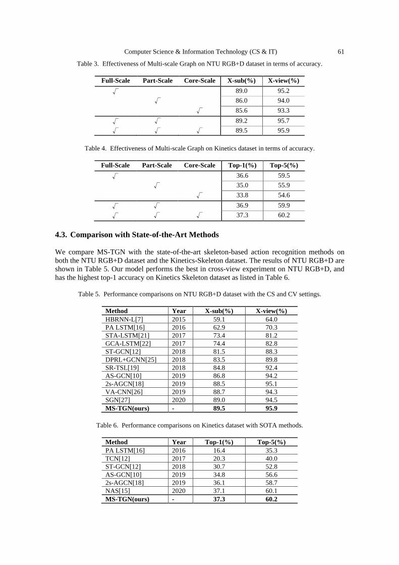
Computer Science & Information Technology (CS & IT) 61
Table 3. Effectiveness of Multi-scale Graph on NTU RGB+D dataset in terms of accuracy.
Full-Scale Part-Scale Core-Scale X-sub(%) X-view(%)
√ 89.0 95.2
√ 86.0 94.0
√ 85.6 93.3
√ √ 89.2 95.7
√ √ √ 89.5 95.9
Table 4. Effectiveness of Multi-scale Graph on Kinetics dataset in terms of accuracy.
Full-Scale Part-Scale Core-Scale Top-1(%) Top-5(%)
√ 36.6 59.5
√ 35.0 55.9
√ 33.8 54.6
√ √ 36.9 59.9
√ √ √ 37.3 60.2
4.3. Comparison with State-of-the-Art Methods
We compare MS-TGN with the state-of-the-art skeleton-based action recognition methods on
both the NTU RGB+D dataset and the Kinetics-Skeleton dataset. The results of NTU RGB+D are
shown in Table 5. Our model performs the best in cross-view experiment on NTU RGB+D, and
has the highest top-1 accuracy on Kinetics Skeleton dataset as listed in Table 6.
Table 5. Performance comparisons on NTU RGB+D dataset with the CS and CV settings.
Method Year X-sub(%) X-view(%)
HBRNN-L[7] 2015 59.1 64.0
PA LSTM[16] 2016 62.9 70.3
STA-LSTM[21] 2017 73.4 81.2
GCA-LSTM[22] 2017 74.4 82.8
ST-GCN[12] 2018 81.5 88.3
DPRL+GCNN[25] 2018 83.5 89.8
SR-TSL[19] 2018 84.8 92.4
AS-GCN[10] 2019 86.8 94.2
2s-AGCN[18] 2019 88.5 95.1
VA-CNN[26] 2019 88.7 94.3
SGN[27] 2020 89.0 94.5
MS-TGN(ours) - 89.5 95.9
Table 6. Performance comparisons on Kinetics dataset with SOTA methods.
Method Year Top-1(%) Top-5(%)
PA LSTM[16] 2016 16.4 35.3
TCN[12] 2017 20.3 40.0
ST-GCN[12] 2018 30.7 52.8
AS-GCN[10] 2019 34.8 56.6
2s-AGCN[18] 2019 36.1 58.7
NAS[15] 2020 37.1 60.1
MS-TGN(ours) - 37.3 60.2

62 Computer Science & Information Technology (CS & IT)
Besides, our model reduces the computational work and parameters, as listed in Table 7. It means
our model is simpler and has a better ability for modelling spatial and temporal features. Why
does our model have fewer parameters and calculation but perform better? In our designed graph,
each node denotes all frame data of a joint, which brings two advantages: (1) TGN extractor only
contains GCN without TCN, which reduces the parameters and calculation. (2) Instead of
extracting alternately, TGN can extract spatial and temporal features at the same time to
strengthen consistence of the spatial and temporal features.
Table 7. Comparisons of the cost of computing with state-of-the-arts. The #Params and FLOPs are
calculated by the tools called THOP (PyTorch-OpCounter) [24].
Method Year X-sub(%) #Params(M) #FLOPs(G)
ST-GCN[12] 2018 81.6 3.1 15.2
AS-GCN[10] 2019 86.8 4.3 17.1
2s-AGCN[18] 2019 88.5 3.5 17.4
NAS[15] 2020 89.4 6.6 36.6
MS-TGN(ours) - 89.5 3.0 15.0
5. CONCLUSIONS
In this paper, we propose MS-TGN model which mainly has two innovations: a model called
TGN to extract temporal and spatial features simultaneously and a multi-scale graph strategy to
obtain both the local features and the contour features. On two large-scale datasets, the proposed
MS-TGN achieves the state-of-the-art accuracy with the least parameters and calculation.
ACKNOWLEDGEMENT
This work is sponsored by the National Natural Science Foundation of China No. 61771281, the
"New generation artificial intelligence" major project of China No. 2018AAA0101605, the 2018
Industrial Internet innovation and development project, and Tsinghua University initiative
Scientific Research Program.
REFERENCES
[1] Bruna, Joan, et al. “Spectral Networks and Locally Connected Networks on Graphs.” ICLR 2014 :
International Conference on Learning Representations (ICLR) 2014, 2014.
[2] Du, Yong, et al. “Skeleton Based Action Recognition with Convolutional Neural Network.” 2015 3rd
IAPR Asian Conference on Pattern Recognition (ACPR), 2015, pp. 579–583.
[3] Du, Yong, et al. “Hierarchical Recurrent Neural Network for Skeleton Based Action Recognition.”
2015 IEEE Conference on Computer Vision and Pattern Recognition (CVPR), 2015, pp. 1110–1118.
[4] Feichtenhofer, Christoph, et al. “Convolutional Two-Stream Network Fusion for Video Action
Recognition.” 2016 IEEE Conference on Computer Vision and Pattern Recognition (CVPR), 2016,
pp. 1933–1941.
[5] Huang, Zhiwu, et al. “Deep Learning on Lie Groups for Skeleton-Based Action Recognition.” 2017
IEEE Conference on Computer Vision and Pattern Recognition (CVPR), 2017, pp. 1243–1252.
[6] Kay, Will, et al. “The Kinetics Human Action Video Dataset.” ArXiv Preprint ArXiv:1705.06950,
2017.
[7] Ke, Qiuhong, et al. “A New Representation of Skeleton Sequences for 3D Action Recognition.” 2017
IEEE Conference on Computer Vision and Pattern Recognition (CVPR), 2017, pp. 4570–4579.
[8] Kim, Tae Soo, and Austin Reiter. “Interpretable 3D Human Action Analysis with Temporal
Convolutional Networks.” 2017 IEEE Conference on Computer Vision and Pattern Recognition
Workshops (CVPRW), 2017, pp. 1623–1631.

Computer Science & Information Technology (CS & IT) 63
[9] Li, Chao, et al. “Co-Occurrence Feature Learning from Skeleton Data for Action Recognition and
Detection with Hierarchical Aggregation.” IJCAI’18 Proceedings of the 27th International Joint
Conference on Artificial Intelligence, 2018, pp. 786–792.
[10] Li, Maosen, et al. “Actional-Structural Graph Convolutional Networks for Skeleton-Based Action
Recognition.” 2019 IEEE/CVF Conference on Computer Vision and Pattern Recognition (CVPR),
2019, pp. 3595–3603.
[11] Li, Shuai, et al. “Independently Recurrent Neural Network (IndRNN): Building A Longer and Deeper
RNN.” 2018 IEEE/CVF Conference on Computer Vision and Pattern Recognition, 2018, pp. 5457–
5466.
[12] Yan, Sijie, et al. “Spatial Temporal Graph Convolutional Networks for Skeleton-Based Action
Recognition.” AAAI, 2018, pp. 7444–7452.
[13] Martinez, Julieta, et al. “On Human Motion Prediction Using Recurrent Neural Networks.” 2017
IEEE Conference on Computer Vision and Pattern Recognition (CVPR), 2017, pp. 4674–4683.
[14] Ofli, Ferda, et al. “Sequence of the Most Informative Joints (SMIJ): A New Representation for
Human Skeletal Action Recognition.” 2012 IEEE Computer Society Conference on Computer Vision
and Pattern Recognition Workshops, 2012, pp. 8–13.
[15] Peng, Wei, et al. “Learning Graph Convolutional Network for Skeleton-Based Human Action
Recognition by Neural Searching.” Proceedings of the AAAI Conference on Artificial Intelligence,
vol. 34, no. 3, 2020, pp. 2669–2676.
[16] Shahroudy, Amir, et al. “NTU RGB+D: A Large Scale Dataset for 3D Human Activity Analysis.”
2016 IEEE Conference on Computer Vision and Pattern Recognition (CVPR), 2016, pp. 1010–1019.
[17] Shi, Lei, et al. “Skeleton-Based Action Recognition With Directed Graph Neural Networks.” 2019
IEEE/CVF Conference on Computer Vision and Pattern Recognition (CVPR), 2019, pp. 7912–7921.
[18] Shi, Lei, et al. “Two-Stream Adaptive Graph Convolutional Networks for Skeleton-Based Action
Recognition.” 2019 IEEE/CVF Conference on Computer Vision and Pattern Recognition (CVPR),
2019, pp. 12026–12035.
[19] Si, Chenyang, et al. “Skeleton-Based Action Recognition with Spatial Reasoning and Temporal Stack
Learning.” Proceedings of the European Conference on Computer Vision (ECCV), 2018, pp. 106–
121.
[20] Si, Chenyang, et al. “An Attention Enhanced Graph Convolutional LSTM Network for Skeleton-
Based Action Recognition.” 2019 IEEE/CVF Conference on Computer Vision and Pattern
Recognition (CVPR), 2019, pp. 1227–1236.
[21] Liu, Jun, et al. “Spatio-Temporal LSTM with Trust Gates for 3D Human Action Recognition.”
European Conference on Computer Vision, 2016, pp. 816–833.
[22] Song, Sijie, et al. “An End-to-End Spatio-Temporal Attention Model for Human Action Recognition
from Skeleton Data.” AAAI’17 Proceedings of the Thirty-First AAAI Conference on Artificial
Intelligence, 2017, pp. 4263–4270.
[23] Cao, Zhe, et al. “OpenPose: Realtime Multi-Person 2D Pose Estimation Using Part Affinity Fields.”
ArXiv Preprint ArXiv:1812.08008, 2018.
[24] Ligeng Zhu. Thop: Pytorch-opcounter. https://github.com/Lyken17/pytorch-OpCounter.
[25] Tang, Yansong, et al. “Deep Progressive Reinforcement Learning for Skeleton-Based Action
Recognition.” 2018 IEEE/CVF Conference on Computer Vision and Pattern Recognition, 2018, pp.
5323–5332.
[26] Zhang, Pengfei, et al. “View Adaptive Neural Networks for High Performance Skeleton-Based
Human Action Recognition.” IEEE Transactions on Pattern Analysis and Machine Intelligence, vol.
41, no. 8, 2019, pp. 1963–1978.
[27] Zhang, Pengfei, et al. “Semantics-Guided Neural Networks for Efficient Skeleton-Based Human
Action Recognition.” 2020 IEEE/CVF Conference on Computer Vision and Pattern Recognition
(CVPR), 2020, pp. 1112–1121.

64 Computer Science & Information Technology (CS & IT)
AUTHORS
Li Tingwei is a master's student in Department of Automation in Tsinghua University,
Beijing, China. She researches action recognition and architecture.
Zhangruiwen is currently pursuing the masterdegree with the Computer Science in
Tsinghua University. He is studying auto-driving and action recognition.
Qing Li, PhD, is a professor of the Department of Automation, Tsinghua University,
P.R. China. He has taught at Tsinghua University since 2000 with major research
interests in system architecture, enterprise modelling and system performance evaluation.
© 2020 By AIRCC Publishing Corporation. This article is published under the Creative Commons
Attribution (CC BY) license.

David C. Wyld et al. (Eds): COMIT, SIPO, AISCA, MLIOB, BDHI - 2020
pp. 65-75, 2020. CS & IT - CSCP 2020 DOI: 10.5121/csit.2020.101606
LOCAL BRANCHING STRATEGY-BASED
METHOD FOR THE KNAPSACK PROBLEM WITH SETUP
Samah Boukhari1, Isma Dahmani2 and Mhand Hifi3
1LaROMaD, USTHB, BP 32 El Alia, 16111 Alger, Algérie 2AMCD-RO, USTHB, BP 32, El Alia, 16111 Bab Ezzouar, Alger, Algerie 3EPROAD EA4669, UPJV, 7 rue du Moulin Neuf, 80000 Amiens, France
ABSTRACT
In this paper, we propose to solve the knapsack problem with setups by combining mixed linear
relaxation and local branching. The problem with setups can be seen as a generalization of 0–1 knapsack problem, where items belong to disjoint classes (or families) and can be selected only
if the corresponding class is activated. The selection of a class involves setup costs and resource
consumptions thus affecting both the objective function and the capacity constraint. The mixed
linear relaxation can be viewed as driving problem, where it is solved by using a special black-
box solver while the local branching tries to enhance the solutions provided by adding a series
of invalid / valid constraints. The performance of the proposed method is evaluated on
benchmark instances of the literature and new large-scale instances. Its provided results are
compared to those reached by the Cplex solver and the best methods available in the literature.
New results have been reached.
KEYWORDS Knapsack, Setups, Local Branching, Relaxation
1. INTRODUCTION
The Knapsack Problem with Setup (namely KPS) can be viewed as a more complex variant of the well-known Knapsack Problem (namely KP), where a set of items is considered that is
divided into a set of classes. Each class is characterized by both fixed cost and fixed capacity
while an item can be selected if the class containing that item is activated. KPS finds its application in many real-world industrial and financial applications, such as order acceptance and
production scheduling. An instance of KPS is characterized by a knapsack capacity C and a set I
= {1,..., m} of disjoint classes associated with items. Each element j belongs to a given class ti =
{1,...,ni } (ni denotes the number of items belonging to the class i, i I) and the j-th item of the i-
th class has a nonnegative profit pij and a weight wij. Furthermore, a nonnegative setup cost fi is incurred and a non-negative setup capacity si is consumed in case items of class i are selected in
the solution. Without loss of generality, we assume that all input parameters have integer values.
The goal of the problem is to maximize the difference between the profits related to the selected items and that related to the fixed costs incurred for setting-up classes without violating the
knapsack capacity constraint. The studied problem has applications in many areas such as
production planning and scheduling (see Chebil and Khemakhem 2015), energy consumption
management (see Della Croce, Salassa, and Scatamacchia 2017), and resource allocation (see

66 Computer Science & Information Technology (CS & IT)
Della Croce, Salassa, and Scatamacchia 2017). The KPS has also a important theoretical status because of its generalization to the classical KP.
The rest of the paper is organized as follows. The related work is exposed in section 2. A
formal description of the knapsack problem with setup is presented in Section 3.1. Section 3.2
describes the greedy initialization procedure that is used for achieving a starting solution. Section
3.3 discusses the standard local branching used for a general mixed integer programming. Section 3.4 presents the adaptation of the local branching for solving KPS. Finally, Section 4 exposes the
experimental part, where the performance of the proposed method is evaluated on two sets of
benchmark instances. The first set, containing small and medium-sized instances, is taken from
the literature where the provided results are compared to the best solution values published in the literature. The second set contains random generated large-scale instances, where the provided
results are compared to those achieved by the Cplex solver.
2. RELATED WORKS
Guignard [10] tackled the setup knapsack by using a Lagrangean decomposition for the setup
knapsack problem, where no restrictions on the non-negativity of both setup cost of each class
and the profit of each item are considered.
A special case of KSP has been studied by Akinc [1] and Altay et al. [2], where only the setup
cost of each class is taken into account (called the fixed charge knapsack problem). In Akinc [1], an exact algorithm has been designed, which is based upon a classical branch-and-bound scheme,
while in Altay et al. [2] the authors tackled the case where items can be fractionated by cross
decomposition.
Michel et al. [11] addressed an extended multiple-class integer knapsack problem with setup. For
that case, the weights associated to items are related to the classes and the total weight is bounded
by both lower and upper weight bounds. Different integer linear programming formulations were proposed and an extended branch-and-bound algorithm that is based upon Horowitz and Sahni
method was proposed such that nonnegative setup costs were favored.
The knapsack problem with setup has been studied by Chebil and Khemakhem [4] who proposed
a dynamic programming procedure, within pseudo-polynomial time complexity. A special
converting formulation was considered in order to reduce the size of the storage capacity, which
remains quite expensive when using such type of approach.
Chebil and Khemakhem [5] designed a special truncated tree-search for approximately solving
KPS. The method applies an avoid duplication technic that consists in reformulating the original problem into a particular integer program. The experimental part showed the effectiveness of that
method, especially the effect of the avoiding duplication technic in terms of improving the quality
of the provided solutions.
Furini et al. [9] developed linear-time algorithms for optimally solving the continuous relaxation
of different integer linear programming formulations of the knapsack with setup. As mentioned in
their experimental part, it has been shown that their algorithms outperform both dynamic programming-based approach and blackbox solver.
Della et al. [7] designed an exact method which handles the structure of the formal description of KSP, where the search process explored the partitioning strategy that is based on splitting the
decision variables into two levels. A fixation strategy has been applied for reducing the current

Computer Science & Information Technology (CS & IT) 67
subproblem to solve while the blackbox solver is applied for solving the reduced subproblem. The experimental part showed that method remains competitive when compared to Chebil and
Khemakhem's [4] dynamic programming method.
Pferschy and al. [12] introduced a new dynamic programming approach which performs better than a previous standard dynamic programming-based procedure; that can be considered as a
good alternative for an exact resolution when combined with an ILP solver.
Chebil et al. [6] proposed a multilevel matheuristic for solving large-scale problem instances of
the knapsack problem with setup and the multiple knapsack version of the problem. The principle
of the method is based (i) on reducing the original instance into a special knapsack instance (each class contains one item) and (ii) on solving the continuous relaxation of the induced problem to
provide a feasible solution for the original problem. In order to enhance the quality of the
solutions reached, a simple tabu list has been incorporated. The experimental part showed that the
proposed method remains competitive when its results were compared to those achieved by the state-of-the-art methods available in the literature.
More recently, Amiri [3] proposed a Lagrangean relaxation-based algorithm for solving the knapsack problem with setup. The method follows the standard adaptation of the Lagrangean
relaxation, where a series of local optimal solutions are provided by using a descent method. The
performance of the method was evaluated on both the standard set of benchmark instances and very large-scale ones (containing till 500 classes and 2 millions of items) and its achieved results
were compared to the best bounds available in the literature.
3. MIXED INTEGER AND LOCAL BRANCHING
3.1. The Model
First, let xij be the decision variable setting equal to 1 if item j of class i is placed in the knapsack, 0 otherwise. Second, let yi denote the setup decision variable that is equal to 1 if the family i is
activated, 0 otherwise. Then, the formal description of SKP (noted PKPS) can be written as
follows:
Maximize
m
iii
m
i
n
jijij yfxp
i
11 1
(1)
Subject to
m
iii
m
i
n
jijij Cysxw
i
11 1
(2)
iiij njIiyx ,...,1 , , (3)
iiij njIiyx ,...,1 , ,0,1,1,0 (4)
Where the objective function (1) maximizes the total profit of the selected items minus the fixed
costs incurred for setting up the selected classes. The constraint (2) ensures that the weight of selected items in the knapsack, including all setup capacities related to the activated classes, does
not exceed the knapsack capacity C. Finally, constraints (3) (representing the precedence
constraints) ensures that an item j is selected only with its activated class j.

68 Computer Science & Information Technology (CS & IT)
3.2. A Starting Solution
A starting solution for KPS can be provided by solving a mixed integer relaxation of the original problem PSKP. Let RPSKP denote the problem provided by relaxing all binary variables, i.e., setting
xij [0, 1] j = 1,…, ni, i I and yi [0, 1], i I such that RPSKP:
Maximize
m
iii
m
i
n
jijij yfxp
i
11 1
Subject to
m
iii
m
i
n
jijij Cysxw
i
11 1
iiij njIiyx ,...,1 , ,
iiij njIiyx ,...,1 , ,1,0,1,0
To provide a constructive approximate solution, we first proceed to fix step by step the variables yi to their binary values and to one the decision variables having a fractional value in PRSKP.
Second, one can observe that a single knapsack problem can be provided by considering the
decision variables xij whose classes are activated, i.e., yi = 1. Third and last, an optimal solution of the induced knapsack problem built in the second step, which allows a feasible starting
solution for PSKP.
The Greedy Constructive Procedure (noted GCP) used, for providing a starting solution, can be described as follows:
- The relaxation RPSKP is optimized by using the simplex method. Then, we collect the current
primal solution by setting ( YX , ) as the achieved configuration.
- Let Y’ denote the binary structure provided by fixing yi to its current integer value and all the fractional variables yi to one,
- Let S be the set of indices of the classes fixed to one: S= {i I | yi=1}.Update C’=C-∑iI si.
- Let PKP be the knapsack problem with capacity C’ and the set of elements xij, iI. Each element
j of class iS is characterized by its profit pij and weight wij . Then, the PKP problem described as
follows: PKP :
Maximize Si
n
jijij
i
xp1
Subject to '1
CxwSi
n
jijij
i
iij njSix ,...,1 , ,1,0
- Let X’ be the optimal solution of PKP. Then, (X’, Y’) denotes the (starting) feasible solution of
PSKP.

Computer Science & Information Technology (CS & IT) 69
Algorithm 1 describes the main steps of GCP that is used for providing a starting solution and used as the core of the proposed method, as shown in the rest of the paper.
3.3. Local Branching
The original Local Branching (LB) has been first introduced by Fischetti and Lodi [8], especially
for efficiently tackling mixed integer formulations of hard combinatorial optimization problems. The solution related to such formulations is often done by calling a black-box solver, like Gurobi,
Cplex and Lingo. Because the aforementioned solvers are not able to optimally solve large-scale
instances, LB can be used as an alternative at least for enhancing the quality of the solutions.
However, since solution procedures using LB-based strategy shown an increasing interest of that method, we propose to solve KPS by using a simple adaptation of LB combined with the greedy
constructive procedure GCP (Algorithm 1). The principle of LB-based algorithm may be
described as follows:
1. Let S be a starting solution affected to the first node of the developed tree.
2. Initialize the first tree using the solution previously generated. 3. Iterative phase:
i Completely resolve the local tree.
ii when the local search terminates, the following two cases are distinguished: a- A better feasible solution has been provided for the local tree structure.
Create a new tree using the aforementioned improved solution like starting
solution (called the reference solution). b- The solution has not been improved, so abort the local branch.
4. Solve the rest of the search tree.
5. Return the best solution found.
3.4. Adaptation of the Local Branching
In order to adapt LB to the studied problem SKP, we need a starting solution for initializing the
first tree, the constraints to use for locally branch on non-searched subspaces and, a blackbox solver for computing the local optimum for each (sub) tree.
Let Y be a feasible reference solution of PKPS provided by the constructive method GCP (cf.
Section 3.2). Let S1 (resp. S0) be the set related to Y containing elements fixed to one (resp. zero),

70 Computer Science & Information Technology (CS & IT)
i.e., S1={i | iI, yi=1} (resp. S0 ={i | iI, yi=1}). Then, for a given nonnegative integer
parameter k, kOpt defines the neighborhood N(Y , k) of the solution Y as the set of the feasible
solutions of PSKP satisfying the following additional local branching constraint:
kyyYYSi
i
Si
i 01
)1()',( (5)
where the two terms of left-hand side count the number of binary variables flipping their value
(with respect to Y ) either from 1 to 0 or from 0 to 1, respectively.
Herein, as used in Fischetti and Lodi [8], the local branching constraint is applied as a branching criterion within an enumerative scheme for PKPS. Indeed, given the incumbent solution Y’, the
solution space associated with the current branching node can be partitioned by separately adding
the following disjunction:
kYY )',( or 1)',( kYY (6)
where k denotes a neighborhood-size parameter.
4. COMPUTATIONAL RESULTS
The objective of the computational investigation is to assess the performance of the Local
Branching-Based Method (LBBM) by comparing their provided bounds (objective values) to the best known bounds available in the literature. LBBM is evaluated on two sets of instances: the
first set, contains 200 small-sized instances, extracted from the literature (cf., Chebil et al. [6])
and a second set, containing 30 large-scale instances, randomly generated following the same generator used by Chebil et al. [6]. Note that the first set (the second set is detailed in section 4.3)
includes 20 groups, where each group contains 10 instances.
These instances are considered as the strongly correlated ones, where they are randomly
generated applying the following generator described below.
1: - Solve PKPS by using the simplex method.
- Let (X’; Y’) be the resulting configuration.
- Call GCP (Algorithm 1) for achieving the starting feasible solution Z0.
2: Stop=0;
3: while (Stop=0) do
4: Solve PKPS with the additional local constraint (Y; Y’) ≤ k, and let (X0; Y0) be the provided
solution with objective value Z0.
5: if (Z0 > Z’) then 6: Set Z’ = Z0.
7: Remove the old branches.
8: Add the new local branch (Y; Y’) ≥ k + 1.
9: Set Y’ = Y0.
10: else
11: Stop=1;
12: end if
13: end while
14: return Z0.
Algorithm 2. Local Branching for KPS

Computer Science & Information Technology (CS & IT) 71
Table 1: Behavior of LBBM on the benchmark instances of the literature: variation of the parameter k
ni N k=2 k=3 k=4 k=5 k=6 k=7 k=8 k=9 k=10
5 500 11004,7 11073,8 11073,8 11073,8 11073,8 11073,8 11073,8 11073,8 11073,8
10 11127,4 11144 11144,6 11144,6 11144,6 11144,6 11144,6 11144,6 11144,6
20 13917,6 13917,6 13917,8 13917,8 13917,8 13917,8 13917,8 13917,8 13917,8
30 13951,8 13952,1 13951,9 13952,2 13952 13952,1 13951,9 13951,7 13952,4
5 1000 19977,8 19977,8 19977,8 19977,8 19977,8 19977,8 19977,8 19977,8 19977,8
10 21943,3 21943,3 21943,3 21943,3 21943,3 21943,3 21943,3 21943,3 21943,3
20 22587,1 22603,5 22629,2 22639,4 22644,1 22648 22648 22648 22648
30 22609 22630,3 22633,5 22647,2 22650,7 22651,1 22650 22650,6 22643,6
5 2500 55185,9 55297,7 55519 55519 55519 55519 55519 55519 55519
10 54840,9 54829,3 54850 54850 54850 54850 54850 54850 54850
20 50128,3 50136,6 50209 50218,7 50245,7 50243,1 50253,4 50244,2 50242,2
30 55445,4 55460,1 55486,5 55514,3 55501,4 55506 55497,1 55505,8 55487,7
5 5000 100302,2 100302,2 100301,9 100302,2 100302,2 100302,2 100302,2 100302,2 100302,2
10 100502,5 100641,9 100645,2 100645,2 100645,2 100649,4 100649,4 100649,4 100649,4
20 100269,8 100544 100630,7 100713,1 100761,1 100774,5 100767,7 100766,9 100761
30 101166,5 101162,2 101183,7 101196,5 101180,8 101177,5 101170,7 101140,4 101152,7
5 10000 221536,1 223128,9 223127,6 223126,4 223126,4 223126,4 223126,4 223126,4 223126,4
10
199177,7 200831,2 201201,8 201227,3 201226,9 201226,9 201227,3 201225,8 201227,9
20
201093 200716,6 201620,8 201522,4 201621,1 201776,9 201776,2 201774,7 201744,8
30
201028,3 200961,6 201486,8 201470,8 201533,3 201520,2 201563,1 201499,7 201485,2
Average 78889,765 79062,735 79176,745 79180,1 79190,86 79199,03 79200,485 79195,605 79192,49
The number of classes varies in the discrete interval {10; 20; 30}.
Number of elements n, related to the number of classes, was fixed to 500, 1000, 2500, 5000 and 10000, respectively.
The number of items ni of each class i I varies in the discrete interval
10,
10
kk
kk where
m
nk and integer.
Both profits and weights were generated as follows; pij is randomly generated in the
discret interval [10; 100] and wij = pij + 10, forming strongly correlated instances.
The setup cost (resp. capacity) of each class i is a random value linking the summation
The setup cost (resp. capacity) of each class i is a random value linking the summation of the profits (resp. weights) of the items belonging to the class; that is,
in
i
iji pef1
1 (resp.
in
i
iji wes1
1 ), where is drawn from the uniform
distribution [0:15, 0:25].
The knapsack capacity )(5.01
Si
n
jij
i
wC
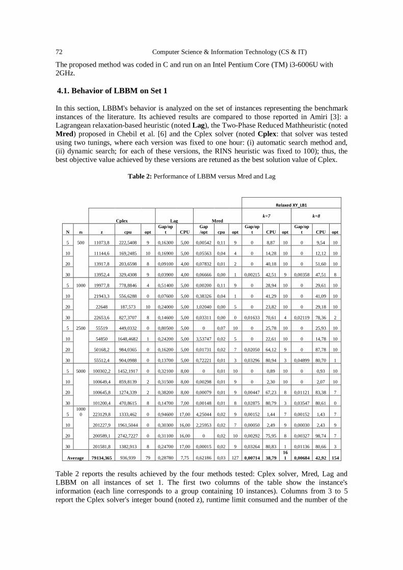
72 Computer Science & Information Technology (CS & IT)
The proposed method was coded in C and run on an Intel Pentium Core (TM) i3-6006U with 2GHz.
4.1. Behavior of LBBM on Set 1
In this section, LBBM's behavior is analyzed on the set of instances representing the benchmark
instances of the literature. Its achieved results are compared to those reported in Amiri [3]: a Lagrangean relaxation-based heuristic (noted Lag), the Two-Phase Reduced Mathheuristic (noted
Mred) proposed in Chebil et al. [6] and the Cplex solver (noted Cplex: that solver was tested
using two tunings, where each version was fixed to one hour: (i) automatic search method and,
(ii) dynamic search; for each of these versions, the RINS heuristic was fixed to 100); thus, the best objective value achieved by these versions are retuned as the best solution value of Cplex.
Table 2: Performance of LBBM versus Mred and Lag
Relaxed XY_LB1
Cplex Lag Mred k=7 k=8
N ni z cpu opt
Gap/op
t CPU
Gap
/opt cpu opt
Gap/op
t CPU opt
Gap/op
t CPU opt
5 500 11073,8 222,5408 9 0,16300 5,00 0,00542 0,11 9 0 8,87 10 0 9,54 10
10
11144,6 169,2485 10 0,16900 5,00 0,05563 0,04 4 0 14,28 10 0 12,12 10
20
13917,8 203,6598 8 0,09100 4,00 0,07832 0,01 2 0 40,18 10 0 51,60 10
30
13952,4 329,4308 9 0,03900 4,00 0,06666 0,00 1 0,00215 42,51 9 0,00358 47,51 8
5 1000 19977,8 778,8846 4 0,51400 5,00 0,00200 0,11 9 0 28,94 10 0 29,61 10
10
21943,3 556,6288 0 0,07600 5,00 0,38326 0,04 1 0 41,29 10 0 41,09 10
20
22648 187,573 10 0,24000 5,00 1,02040 0,00 5 0 23,82 10 0 29,18 10
30
22653,6 827,3707 8 0,14600 5,00 0,03311 0,00 0 0,01633 70,61 4 0,02119 78,36 2
5 2500 55519 449,0332 0 0,80500 5,00 0 0,07 10 0 25,78 10 0 25,93 10
10
54850 1648,4682 1 0,24200 5,00 3,53747 0,02 5 0 22,61 10 0 14,78 10
20
50168,2 984,0365 0 0,16200 5,00 0,01731 0,02 7 0,02050 64,12 9 0 87,78 10
30
55512,4 904,0988 0 0,13700 5,00 0,72221 0,01 3 0,03296 80,94 3 0,04899 80,70 1
5 5000 100302,2 1452,1917 0 0,32100 8,00 0 0,01 10 0 0,89 10 0 0,93 10
10
100649,4 859,8139 2 0,31500 8,00 0,00298 0,01 9 0 2,30 10 0 2,07 10
20
100645,8 1274,339 2 0,38200 8,00 0,00079 0,01 9 0,00447 67,23 8 0,01121 83,38 7
30
101200,4 470,8615 8 0,14700 7,00 0,00148 0,01 8 0,02875 80,79 3 0,03547 80,61 0
5
1000
0 223129,8 1333,462 0 0,94600 17,00 4,25044 0,02 9 0,00152 1,44 7 0,00152 1,43 7
10
201227,9 1961,5044 0 0,30300 16,00 2,25953 0,02 7 0,00050 2,49 9 0,00030 2,43 9
20
200589,1 2742,7227 0 0,31100 16,00 0 0,02 10 0,00292 75,95 8 0,00327 98,74 7
30
201581,8 1382,913 8 0,24700 17,00 0,00015 0,02 9 0,03264 80,83 1 0,01136 80,66 3
Average 79134,365 936,939 79 0,28780 7,75 0,62186 0,03 127 0,00714 38,79
16
1 0,00684 42,92 154
Table 2 reports the results achieved by the four methods tested: Cplex solver, Mred, Lag and
LBBM on all instances of set 1. The first two columns of the table show the instance's
information (each line corresponds to a group containing 10 instances). Columns from 3 to 5
report the Cplex solver's integer bound (noted z), runtime limit consumed and the number of the

Computer Science & Information Technology (CS & IT) 73
optimal solution values matched by the Cplex. Columns 6 and 7 display the average Gap
(computed as follows: 100
opt
procedureopt
z
zzGap ) achieved by Lag and its runtime limit
(extracted from Amiri [3]. Columns from 8 to 10 tally the average Mred's Gap, its average runtime limit and the number of optimal solution values matched by Mred. Finally, column from
11 to 13 (resp. from 14 to 16) show the LBBM's average Gap with k = 7 (resp. k = 8), its related
average runtime and the number of the optimal solution values matched by the algorithm.
In what follows, we comment on the results reported in Table 2, where we compare the number
of results obtained by the proposed method LBBM (the solution values) with the best solution
values provided by the other three methods. On the one hand, LBBM with k = 7 (resp. k = 8) achieves an average Gap of 0.00714 (resp. 0.00684) while Lag's average Gap is equal to 0.28780
and that of Mred is more greater (0.62186). On the other hand, Cplex matches 79 optimal values
over the 200 instances of Set 1 (representing a percentage of 39.5%), Mred provides 127 optimal values (representing a percentage of 63.5%) whereas LBBM matches 161 optimal values for k =
7 (representing a percentage of 80.5%) and 154 ones for k = 8 (representing a percentage of
77%). Finally, even LBBM's average runtime remains higher when compared to those consumed
by Lag and Mred, it remains very reasonable for a method using a local branching strategy.
4.2. Behavior of LBBM on the Instances of Set 2
Because Chebil et al. [6]'s instances are note available, we then considered thirty instances
representing more largest benchmark instances (these instances are publicly available for other
researchers in the domain): the number of classes (m) varies in the discrete interval {50; 150;
300}, the total number of items of each class (ni, i I) varies in the discrete interval {10000; 100000}, where five instances are considered for each of the six groups. Herein, LBBM's
behavior is analyzed on these instances, where its achieved results are also compared to those
achieved by the Cplex solver. Table 3 reports the solution values achieved by Cplex solver (its runtime limit was fixed to 3600 seconds) and LBBM on the instances of Set 2. From the table,
one can observe what follows:
1. LBBM remains competitive when comparing its results to those achieved by the Cplex solver.
2. LBBM is able to provide ten better average bounds with k = 7 (column 5 in bold-space) than
those achieved by Cplex. In this case, LBBM's global average bound is equal to 1472611.17 for k = 7 (resp. 1472487.97 for k = 8) while Cplex's global average bound is equal to
1472310.57.
3. For k = 7, LBBM's average Gap is equal to -0.020 (column 7, last line) and it is equal to -
0.012 for k = 8 (column 10, last line) which means that LBBM is capable to improve globally the bounds achieved by the Cplex solver by consuming a smaller runtime (in some cases, it
needs only twentieth than the average runtime required by the Cplex).
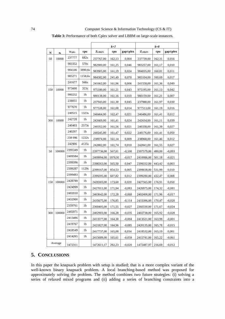
74 Computer Science & Information Technology (CS & IT)
Table 3: Performance of both Cplex solver and LBBM on large-scale instances.
k=7 k=8
N ni zCplex cpu ZLBKPS cpu gap/cplex ZLBKPS cpu gap/cplex
50 10000 237777 682s 237767,00 162,13 0,004 237739,00 162,31 0,016
983352 570s 982900,00 161,25 0,046 983257,00 161,17 0,010
984146 3890,6s 983905,00 161,19 0,024 984035,00 160,81 0,011
985271 1158,6s 984582,00 241,49 0,070 985104,00 160,69 0,017
241677 946s 241662,00 161,96 0,006 241558,00 161,36 0,049
150 10000 975600 323s 975180,00 161,21 0,043 975195,00 161,13 0,042
980232 1h 980138,00 161,16 0,010 980159,00 161,21 0,007
238051 1h 237943,00 161,30 0,045 237980,00 161,97 0,030
977670 1h 977538,00 161,08 0,014 977513,00 161,19 0,016
240515 1323s 240464,00 162,47 0,021 240486,00 161,41 0,012
300 10000 242728 1h 242669,00 161,41 0,024 242634,00 161,11 0,039
240403 2573s 240352,00 161,56 0,021 240338,00 161,39 0,027
240297 1h 240245,00 161,47 0,022 240176,00 161,41 0,050
238 996 1222s 238974,00 161,14 0,009 238968,00 161,46 0,012
242906 4125s 242882,00 161,74 0,010 242841,00 161,55 0,027
50 100000 2395349 1h 2397736,00 567,01 -0,100 2397579,00 480,00 -0,093
2409584 1h 2409994,00 1976,91 -0,017 2410086,00 501,18 -0,021
2399396 1h 2398263,00 565,50 0,047 2399332,00 443,42 0,003
2399287 1129s 2399167,00 854,53 0,005 2399038,00 531,99 0,010
2399483 1h 2399205,00 607,82 0,012 2399280,00 432,47 0,008
150 100000 2428789 1h 2428303,00 173,60 0,020 2427565,00 176,91 0,050
2424999 1h 2427011,00 171,94 -0,083 2426975,00 174,32 -0,081
2402010 1h 2403642,00 172,28 -0,068 2402408,00 171,96 -0,017
2432900 1h 2435675,00 176,85 -0,114 2433396,00 170,47 -0,020
2359761 1h 2360405,00 171,55 -0,027 2360330,00 171,67 -0,024
300 100000 2402071 1h 2402903,00 166,28 -0,035 2402738,00 165,92 -0,028
2413486 1h 2413577,00 164,30 -0,004 2413521,00 163,99 -0,001
2419767 1h 2421827,00 164,96 -0,085 2420135,00 165,78 -0,015
2418549 1h 2417737,00 165,08 0,034 2418532,00 165,19 0,001
2414265 1h 2415689,00 165,61 -0,059 2415741,00 165,22 -0,061
Average
1472311
1472611,17 292,23 -0,020 1472487,97 216,69 -0,012
5. CONCLUSIONS
In this paper the knapsack problem with setup is studied; that is a more complex variant of the
well-known binary knapsack problem. A local branching-based method was proposed for approximately solving the problem. The method combines two future strategies: (i) solving a
series of relaxed mixed programs and (ii) adding a series of branching constraints into a

Computer Science & Information Technology (CS & IT) 75
developed tree-search. Both strategies cooperate for creating a tree-search, where each path corresponds to adding a series of constraints related to the current or improved solutions. The
performance of proposed method was analyzed on two sets of instances containing small and
large-scale instances. According to the experimental part, the proposed method remains
competitive, where it outperforms methods available in the literature and is able to provide improved solutions for large-scale instances.
REFERENCES [1] U. Akinc, (2006) “Approximate and exact algorithms for the fixed-charge knapsack problem”,
European Journal of Operational Research, Vol. 170, No 2, pp 363-375.
[2] N. Altay, JR. Robinson, E. Powell, and K. M. Bretthauer, (2008) “Exact and heuristic solution
approaches for the mixed integer setup knapsack problem”, European Journal of Operational
Research, Vol. 190, No 3, pp 598-609.
[3] A. Amiri, (2019) “A Lagrangean based solution algorithm for the knapsack problem with setups”,
Expert Systems with Applications, Vol. 143, pp113077. [4] K. Chebil, and M. Khemakhem, (2015) “A dynamic programming algorithm for the knapsack
problem with setup”, Computers and Operations Research, Vol. 64, pp 40-50.
[5] K. Chebil and M. Khemakhem, (2016) “A tree search based combination heuristic for the knapsack
problem with setup”, Computers and Industrial Engineering, Vol. 99, pp 280-286.
[6] K. Chebil, R. Lahyani, M. Khemakhem, and L. C. Coelho, (2019) “Matheuristics for solving the
Multiple Knapsack Problem with Setup”, Computers and Industrial Engineering, Vol. 129, pp 76-89.
[7] C.F. Della, , F. Salassa, and R. Scatamacchia, (2017) “An exact approach for the 0-1 knapsack
problem with setups”, Computers and Operations Research, Vol. 80, pp 61-67.
[8] M. Fischetti and A.Lodi , (2003) “Local branching, Mathematical Programming”, Vol. 98, pp. 23{47.
[9] F. Furini, M. Monaci and E. Traversi, (2017) “Exact algorithms for the knapsack problem with
setup”, Technical report, Universit Paris Dauphine. [10] M. Guignard, (1993) “Solving makespan minimization problems with lagrangean decomposition”,
Discrete Applied Mathematics, Vol. 42, no 1, pp. 17-29.
[11] S. Michel, N. Perrot, and F. Vanderbeck, (2017) “Knapsack problems with setups”, European
Journal of Operational Research, Vol. 196, no 3, pp. 909-918.
[12] U. Pferschy, R. Scatamacchia, (2018) “Improved dynamic programming and approximation results
for the knapsack problem with setups“, International Transactions in Operational Research, Vol. 25,
no 2, pp. 667-682.
© 2020 By AIRCC Publishing Corporation. This article is published under the Creative Commons
Attribution (CC BY) license.

76 Computer Science & Information Technology (CS & IT)

David C. Wyld et al. (Eds): COMIT, SIPO, AISCA, MLIOB, BDHI - 2020
pp. 77-91, 2020. CS & IT - CSCP 2020 DOI: 10.5121/csit.2020.101607
LINEAR REGRESSION EVALUATION OF
SEARCH ENGINE AUTOMATIC SEARCH
PERFORMANCE BASED ON HADOOP AND R
Hong Xiong
University of California – Los Angeles, Los Angeles, CA, USA
ABSTRACT The automatic search performance of search engines has become an essential part of measuring
the difference in user experience. An efficient automatic search system can significantly improve
the performance of search engines and increase user traffic. Hadoop has strong data integration
and analysis capabilities, while R has excellent statistical capabilities in linear regression. This
article will propose a linear regression based on Hadoop and R to quantify the efficiency of the automatic retrieval system. We use R's functional properties to transform the user's search
results upon linear correlations. In this way, the final output results have multiple display forms
instead of web page preview interfaces. This article provides feasible solutions to the drawbacks
of current search engine algorithms lacking once or twice search accuracies and multiple types
of search results. We can conduct personalized regression analysis for user’s needs with public
datasets and optimize resources integration for most relevant information.
KEYWORDS Hadoop, R, search engines, linear regression, machine learning.
1. INTRODUCTION
With the rapid development of the Internet, the Internet has gradually penetrated all aspects of users' lives and work. People can search and obtain the information they want through the
information system platform [1]. In traditional information retrieval systems, people tend to focus on retrieval techniques, algorithms, and how to help users better provide information that matches keywords. However, the background and purpose of the user search are different. Traditional information retrieval systems cannot meet the requirements of users. With the emergence of social search platforms such as social media and social question and answer systems, users are no longer limited to the "human-machine" interaction model. With social services such as making friends, cooperating, sharing, communicating, and publishing content, users can quickly and
accurately find information to meet their needs [2]. The search engine is a necessary function for the convenience of the source users to use the website to construct the website. It is also a useful tool for studying the website users' behaviour. New Competitiveness believes that efficient site search can allow users to find target information quickly and accurately, thereby more effectively promoting the sales of products/services. Through in-depth analysis of website visitors' search behaviour, it is helpful for further development of a more effective network marketing strategy. Therefore, for essential information
websites with rich content and online sales websites with rich product lines, it is far from enough to provide general full-text search. It is necessary to develop advanced search functions that can

78 Computer Science & Information Technology (CS & IT)
achieve personalized needs and reflect on the crucial aspects of the website's network marketing function. The search engine has become an indispensable tool of the Internet, which can help people find
the content and information they want more quickly, improve the efficiency of doing things, and efficiently use Internet resources. However, users now generally have secondary searches when they use search engines. This phenomenon is the fundamental basis of the writing of this paper. Moreover, many secondary searches are further attributive restrictions on nouns, showing that the search results that users need are no longer just the abbreviated content of the webpage but also require the participation of rich elements. However, due to our lack of professional knowledge and understanding of
search engines, we cannot further analyse the underlying causes and propose practical solutions. We can only hypothesize and demonstrate our conjectures. This work needs to be further improved, and we look forward to seeing perfect theoretical research results from other scholars. Nevertheless, this paper provides a feasible algorithm combined with Hadoop and R for optimizing resource integration of search engines, along with a program frame for the realization of this algorithm.
In the second section, this paper will discuss related works about optimizations of search engine algorithms and their drawbacks. In the third section, we will discuss the properties of R and Hadoop separately and their integration basis. In the fourth section, we will propose a R-based Hadoop vision for algorithm optimization, reason of choosing linear regression, market value of this proposal, program frame and related experiments. In the final section, we will summarize all the assumptions and limitations of our proposal and analyse the next step of our research.
2. RELATED WORKS
Performance evaluation has always been one of the core issues of network information retrieval
research. Traditional evaluation methods require a lot of human resources and material resources. Based on user behaviour analysis, a method for automatically evaluating search engine performance is proposed [3]. The navigation type queries the test set and automatically annotates the standard answers corresponding to the query [4]. Experimental results show that this method can achieve a basic performance. This consistent evaluation effect dramatically reduces the workforce and material resources required for evaluation and speeds up the evaluation feedback cycle.
The retrieval system's evaluation problem has always been one of the core problems in information retrieval research. Saracevic pointed out: "Evaluation problem is in such an important position in the research and development process of information retrieval that any new method and their evaluation. The way is integrated." Kent first proposed the precision rate-recall rate information retrieval evaluation framework. Subsequently, research institutions affiliated with the US government began to strongly support research on retrieval evaluation and the United Kingdom's Cranfield project in the late 1950s. The evaluation plan based on query sample
sets, standard answer sets, and corpus established in the mid-1960s truly made information retrieval an empirical discipline and thus established the core of evaluation in information retrieval research. Status and its evaluation framework are generally called the Cranfield-like approach (A Cranfield-like approach) [5]. The Cranfield method points out that the evaluation of an information retrieval system should consist of the following links:
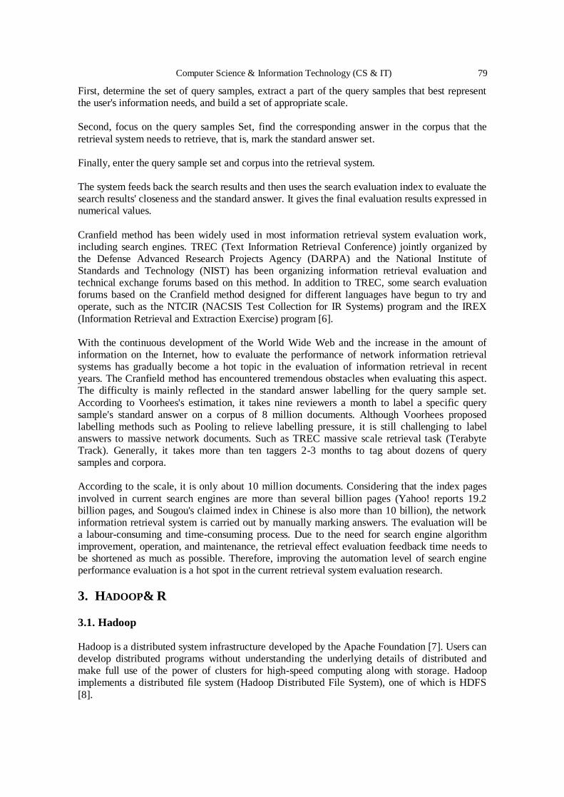
Computer Science & Information Technology (CS & IT) 79
First, determine the set of query samples, extract a part of the query samples that best represent the user's information needs, and build a set of appropriate scale. Second, focus on the query samples Set, find the corresponding answer in the corpus that the
retrieval system needs to retrieve, that is, mark the standard answer set. Finally, enter the query sample set and corpus into the retrieval system. The system feeds back the search results and then uses the search evaluation index to evaluate the search results' closeness and the standard answer. It gives the final evaluation results expressed in numerical values.
Cranfield method has been widely used in most information retrieval system evaluation work, including search engines. TREC (Text Information Retrieval Conference) jointly organized by the Defense Advanced Research Projects Agency (DARPA) and the National Institute of Standards and Technology (NIST) has been organizing information retrieval evaluation and technical exchange forums based on this method. In addition to TREC, some search evaluation forums based on the Cranfield method designed for different languages have begun to try and operate, such as the NTCIR (NACSIS Test Collection for IR Systems) program and the IREX
(Information Retrieval and Extraction Exercise) program [6]. With the continuous development of the World Wide Web and the increase in the amount of information on the Internet, how to evaluate the performance of network information retrieval systems has gradually become a hot topic in the evaluation of information retrieval in recent years. The Cranfield method has encountered tremendous obstacles when evaluating this aspect. The difficulty is mainly reflected in the standard answer labelling for the query sample set.
According to Voorhees's estimation, it takes nine reviewers a month to label a specific query sample's standard answer on a corpus of 8 million documents. Although Voorhees proposed labelling methods such as Pooling to relieve labelling pressure, it is still challenging to label answers to massive network documents. Such as TREC massive scale retrieval task (Terabyte Track). Generally, it takes more than ten taggers 2-3 months to tag about dozens of query samples and corpora. According to the scale, it is only about 10 million documents. Considering that the index pages
involved in current search engines are more than several billion pages (Yahoo! reports 19.2 billion pages, and Sougou's claimed index in Chinese is also more than 10 billion), the network information retrieval system is carried out by manually marking answers. The evaluation will be a labour-consuming and time-consuming process. Due to the need for search engine algorithm improvement, operation, and maintenance, the retrieval effect evaluation feedback time needs to be shortened as much as possible. Therefore, improving the automation level of search engine performance evaluation is a hot spot in the current retrieval system evaluation research.
3. HADOOP& R
3.1. Hadoop
Hadoop is a distributed system infrastructure developed by the Apache Foundation [7]. Users can develop distributed programs without understanding the underlying details of distributed and make full use of the power of clusters for high-speed computing along with storage. Hadoop implements a distributed file system (Hadoop Distributed File System), one of which is HDFS
[8].

80 Computer Science & Information Technology (CS & IT)
HDFS has the characteristics of high fault tolerance and is designed to be deployed on low-cost hardware. It provides high throughput to access application data, and it is suitable for large dataset applications. HDFS relaxes POSIX requirements and can access data in the file system in the form of streaming access. The core design of the Hadoop framework is HDFS and
MapReduce. HDFS provides storage for massive amounts of data, while MapReduce provides calculations for massive amounts of data [9].
3.2. R
R provides a wide variety of statistical (linear and nonlinear modelling, classical statistical tests, time-series analysis, classification, clustering) and graphical techniques. Moreover, it is highly extensible. The S language is often the vehicle of choice for research in statistical methodology, and R provides an Open Source route to participation in that activity [10]. Also, R is now the most widely used statistical software in academic science and it is rapidly expanding into other fields such as finance. R is almost limitlessly flexible and powerful [11].
One of R’s strengths is the ease with which well-designed publication-quality plots can be produced, including mathematical symbols and formulae where needed. Great care has been taken over the defaults for the minor design choices in graphics, but the user retains full control [12]. R is an integrated suite of software facilities for data manipulation, calculation, and graphical display [13]. It includes an effective data handling and storage facility.
I. a suite of operators for calculations on arrays, in particular matrices,
II. an extensive, coherent, integrated collection of intermediate tools for data analysis, III. graphical facilities for data analysis and display either on-screen or on hardcopy, and IV. a well-developed, simple, and effective programming language, including conditionals,
loops, user-defined recursive functions, and input and output facilities. The term “environment” is intended to characterize it as a thoroughly planned and coherent
system, rather than an incremental accretion of particular and inflexible tools, as is frequently the case with other data analysis software. Like S, R is designed around an actual computer language, and it allows users to add additional functionality by defining new functions. Much of the system is itself written in the R dialect of S, making it easy for users to follow the algorithmic choices made. For computationally intensive tasks, C, C++, and Fortran code can be linked and called at run time. Advanced users can write C
code to manipulate R objects directly [14]. Many users think of R as a statistics system [15]. We prefer to think of it as an environment within which statistical techniques are implemented. R can be extended (easily) via packages. There are about eight packages supplied with the R distribution, and many more are available through the CRAN family of Internet sites covering an extensive range of modern statistics.
For hardware reasons (disk space, CPU performance) there is currently no search facility at the R master webserver itself. However, due to the highly active R user community (without which R would not be what it is today) there are other possibilities to search in R web pages and mail archives: An R site search is provided by Jonathan Baron at the University of Pennsylvania, United States. This engine lets you search help files, manuals, and mailing list archives [16].

Computer Science & Information Technology (CS & IT) 81
Rseek is provided by Sasha Goodman at Stanford University. This engine lets you search several R-related sites and can easily be added to the toolbar of popular browsers [17]. The Nabble R Forum is an innovative search engine for R messages. As it has been misused for
spam injection, it is nowadays severely filtered. In addition, its gateway to R-help is sometimes not bidirectional, so we do not recommend it for posting (rather at most for browsing) [18].
3.3. R and Hadoop Integration Base
R is a complete data processing, calculation, and drawing software system. The idea of R is it can
provide some integrated statistical tools, but a more considerable amount is that it provides various mathematical calculations and statistical calculation functions so that users can flexibly analyse data and even create new ones that meet their needs [19]. Hadoop is a framework for distributed data and computing. It is good at storing large amounts of semi-structured data sets. Data can be stored randomly, so the failure of a disk will not cause data loss. Hadoop is also incredibly good at distributed computing-quickly processing large data sets
across multiple machines [20]. Hadoop can be widely used in big data processing applications thanks to its natural advantages in data extraction, transformation, and loading (ETL). Hadoop has distributed architecture that puts the big data processing engine as close to the storage as possible, which is relatively suitable for batch processing operations such as ETL. The batch processing results of similar operations can go directly to storage. The MapReduce function of Hadoop realizes the fragmentation of a single task. It sends the fragmented task (Map) to multiple nodes and then loads (Reduce) into the data
warehouse in the form of a single data set. When users search for information, do they only need a web-linked display, or do they need multimedia materials and resources such as pictures, videos, and audio-visual [21]?
4. R BASED HADOOP For customers' keywords, Hadoop can respond quickly to the attached resources, but it cannot provide rich content and forms. R can compensate for this weakness. This issue is the form we want to explore today. It is possible to use R's functional computing capabilities based on Hadoop to quickly mobilize various forms of network resources to provide users with various high-value information.
In the global search, it is the display of web links. It pushes diversified information such as pictures and videos for users to choose personalized search, personalized settings, personalized data analysis, and personalized data output. Therefore, we might need to conduct forward-looking questions and answers on customer search requirements in advance, understand the main search requirements areas or directions of customers and reduce pushes in other areas. The current search engines are all searched by the Hadoop algorithm. Now we will find out
whether Hadoop can allow users to search for the desired results only once by using the search user usage of some search engines.
4.1. Linear Regression in Data Processing
In this paper, we choose linear regression as main method for the following reasons:
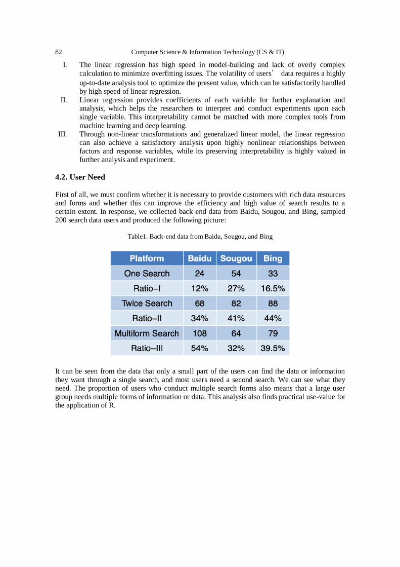
82 Computer Science & Information Technology (CS & IT)
I. The linear regression has high speed in model-building and lack of overly complex
calculation to minimize overfitting issues. The volatility of users’ data requires a highly
up-to-date analysis tool to optimize the present value, which can be satisfactorily handled by high speed of linear regression.
II. Linear regression provides coefficients of each variable for further explanation and analysis, which helps the researchers to interpret and conduct experiments upon each single variable. This interpretability cannot be matched with more complex tools from
machine learning and deep learning. III. Through non-linear transformations and generalized linear model, the linear regression
can also achieve a satisfactory analysis upon highly nonlinear relationships between factors and response variables, while its preserving interpretability is highly valued in further analysis and experiment.
4.2. User Need
First of all, we must confirm whether it is necessary to provide customers with rich data resources and forms and whether this can improve the efficiency and high value of search results to a certain extent. In response, we collected back-end data from Baidu, Sougou, and Bing, sampled 200 search data users and produced the following picture:
Table1. Back-end data from Baidu, Sougou, and Bing
It can be seen from the data that only a small part of the users can find the data or information they want through a single search, and most users need a second search. We can see what they need. The proportion of users who conduct multiple search forms also means that a large user group needs multiple forms of information or data. This analysis also finds practical use-value for the application of R.

Computer Science & Information Technology (CS & IT) 83
Figure 1. Baidu’s user data about search time ratios
First is Baidu's user data. We can see that a search can only meet the needs of one over ten of the users. Users with need for a secondary search and compound search comprise 88% of the user community. It is essential for search engines to discover potential customer groups. They need a search engine to provide more efficient service after typing keywords, which shows information and data to meet users' needs.
Figure 2. Sougou’s user data about search time ratios
Second is the user data from Sougou. Here, we can see that 27% of the users perform a search and get the resources they need. However, there are still 32% of the users needing to search for a variety of forms. 41% of the users need to undertake a secondary search, which means that more
than two-thirds of the user also has the search efficiency room for improvement.

84 Computer Science & Information Technology (CS & IT)
Figure 3. Bing’s user data about search time ratios
Bing and Baidu, Sougou data have something in common: one time of search can only meet a few people's needs, secondary search occupies the most proportion. This kind of situation implies to search engine providers that users might abandon their search scheme and urgently need more advanced search solution to meet their new requirements.
12%
34%
54%
27%
41%
32%
16.5%
44%
39.5%
12%
16.5%
27%
32%
34%
39.5%
41%
44%
54%
Baidu Bing Sougou
Variable
Valu
e
Platform
Ratio−I
Ratio−II
Ratio−III
Figure 4. Line Chart of user data comparison among Baidu, Sougou, and Bing
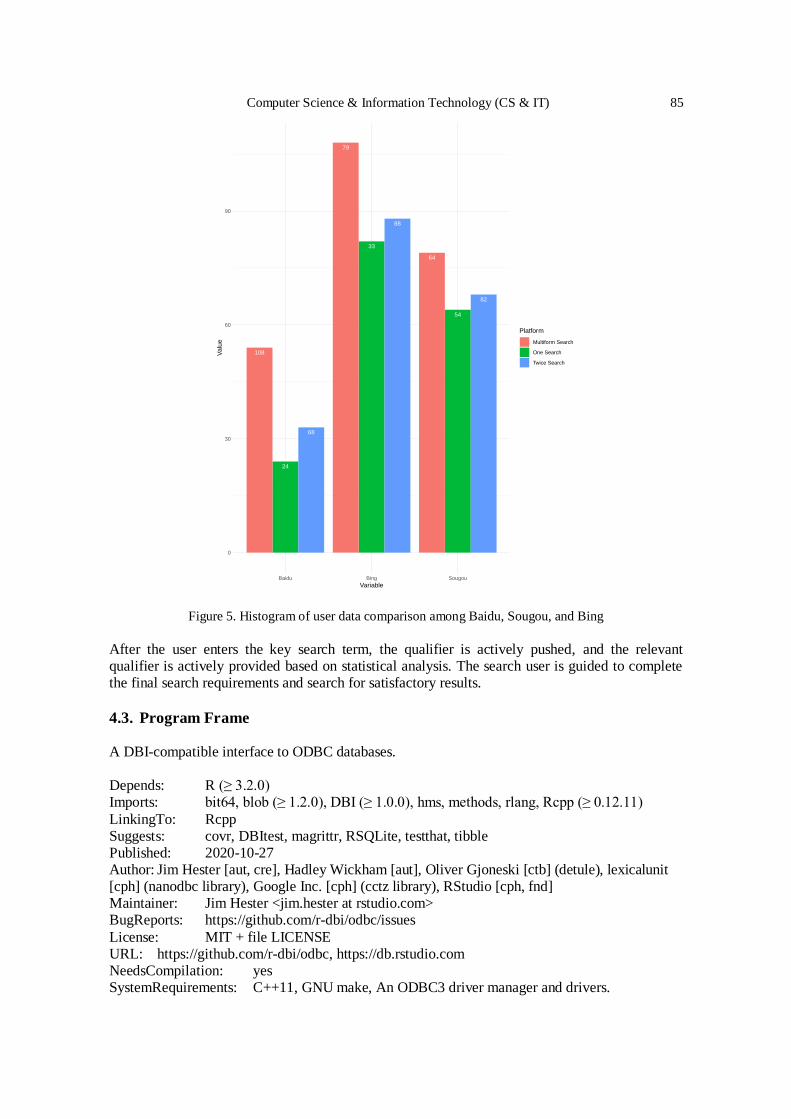
Computer Science & Information Technology (CS & IT) 85
24
68
108
54
82
64
33
88
79
0
30
60
90
Baidu Bing Sougou
Variable
Valu
e
Platform
Multiform Search
One Search
Twice Search
Figure 5. Histogram of user data comparison among Baidu, Sougou, and Bing
After the user enters the key search term, the qualifier is actively pushed, and the relevant qualifier is actively provided based on statistical analysis. The search user is guided to complete the final search requirements and search for satisfactory results.
4.3. Program Frame
A DBI-compatible interface to ODBC databases. Depends: R (≥ 3.2.0) Imports: bit64, blob (≥ 1.2.0), DBI (≥ 1.0.0), hms, methods, rlang, Rcpp (≥ 0.12.11)
LinkingTo: Rcpp Suggests: covr, DBItest, magrittr, RSQLite, testthat, tibble Published: 2020-10-27 Author: Jim Hester [aut, cre], Hadley Wickham [aut], Oliver Gjoneski [ctb] (detule), lexicalunit [cph] (nanodbc library), Google Inc. [cph] (cctz library), RStudio [cph, fnd] Maintainer: Jim Hester <jim.hester at rstudio.com> BugReports: https://github.com/r-dbi/odbc/issues
License: MIT + file LICENSE URL: https://github.com/r-dbi/odbc, https://db.rstudio.com NeedsCompilation: yes SystemRequirements: C++11, GNU make, An ODBC3 driver manager and drivers.
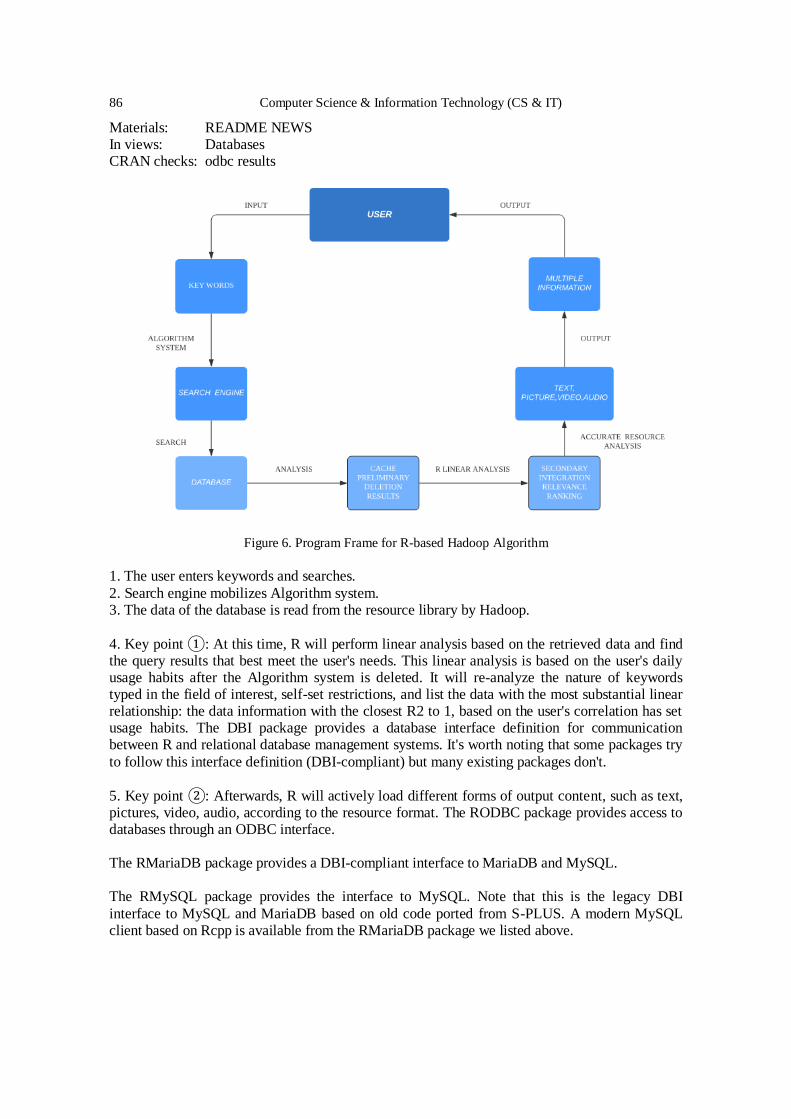
86 Computer Science & Information Technology (CS & IT)
Materials: README NEWS In views: Databases CRAN checks: odbc results
Figure 6. Program Frame for R-based Hadoop Algorithm
1. The user enters keywords and searches.
2. Search engine mobilizes Algorithm system. 3. The data of the database is read from the resource library by Hadoop.
4. Key point ①: At this time, R will perform linear analysis based on the retrieved data and find the query results that best meet the user's needs. This linear analysis is based on the user's daily usage habits after the Algorithm system is deleted. It will re-analyze the nature of keywords typed in the field of interest, self-set restrictions, and list the data with the most substantial linear relationship: the data information with the closest R2 to 1, based on the user's correlation has set usage habits. The DBI package provides a database interface definition for communication between R and relational database management systems. It's worth noting that some packages try
to follow this interface definition (DBI-compliant) but many existing packages don't.
5. Key point ②: Afterwards, R will actively load different forms of output content, such as text, pictures, video, audio, according to the resource format. The RODBC package provides access to databases through an ODBC interface. The RMariaDB package provides a DBI-compliant interface to MariaDB and MySQL. The RMySQL package provides the interface to MySQL. Note that this is the legacy DBI
interface to MySQL and MariaDB based on old code ported from S-PLUS. A modern MySQL client based on Rcpp is available from the RMariaDB package we listed above.

Computer Science & Information Technology (CS & IT) 87
6. Display colourful forms through search engine output interface. The odbc package provides a DBI-compliant interface to drivers of Open Database Connectivity (ODBC), which is a low-level, high-performance interface that is designed specifically for relational data stores.
The RPresto package implements a DBI-compliant interface to Presto, an open source distributed SQL query engine for running interactive analytic queries against data sources of all sizes ranging from gigabytes to petabytes. 7. The user obtains the required information. 8. End of search task.
4.4. Experiment
Our experiment focuses on whether the search accuracy could be improved with our R-based Hadoop system. We use the same scale according to our previous back-end data from Baidu, Sougou, and Bing: “Once Search”, “Twice Search”, and “Multiform Search”. Ideally, we hope to prioritize the increase in the ratio of “Once Search” and “Twice Search”,and reduce the ratio of
“Multiform Search” since this form of search means an inefficient experience for the users. With our training data, we read the database data from the resource library by Hadoop, which is a series of web links according to the entered keywords by users. Then we mark the response variable according to the actual user behaviors. A link would be marked as “Once Search” if the user runs one search and clicks the link, “Twice Search” if the user runs two searches and clicks the link, “Multiform Search” if the user runs more than two
searches or make edits, and clicks the link, “Futile Search” if the user doesn’t click the link. However, our analysis will focus primarily on the first three categories of our response variable since “Futile Search” doesn’t indicate a successful search in our model, but these failed attempts, with huge data, might contain information that helps improve our model accuracy. Then we add parameters/predictors for our response variable from two parts. The first part is based on the properties of the web link, and we use the historical click rate, the relative popularity of the publisher, existence of image/audio/ external links, etc. The second part is based on usage
habits from users, and we use usage frequencies of certain search engines along with personal settings, etc. After finishing the data collection and organization, we conduct near-zero-variance predictors elimination, highly correlated predictors elimination, centering and scaling of predictors, linear regression summary, and principal component analysis (PCA) to filter the most significant predictors. Then, with repeated cross-validation, we apply four machine learning models based on training data: KNN, LDA, QDA, and Multinomial logistic regression, and take a model ensemble based on the majority vote. After the training of our ensemble models, we use
test data from our previous data to see if the ratios of “Once Search” and “Twice Search” increase. The followings are our test results after removing the “Futile Search” and selecting the same total size for our first three categories:

88 Computer Science & Information Technology (CS & IT)
Table 2. Search Time Ratios from Baidu, Sougou, and Bing after linear regression
Platform
One Search
Baidu
Ratio−I
Sougou
Twice Search
Bing
Ratio−II
Multiform Search
Ratio−III
55
27.5%
42
21%
103
51.5%
57
28.5%
75
37.5%
68
34%
75
37.5%
66
33%
59
29.5%
27.5%
21%
51.5%
28.5%
37.5%
34%
37.5%
33%
29.5%
21%
27.5%
28.5%
29.5%
33%
34%
37.5%
51.5%
Baidu Bing Sougou
Variable
Valu
e
Platform
Ratio−I
Ratio−II
Ratio−III
Figure 7. Line Chart of user data comparison among Baidu, Sougou, and Bing after linear regression
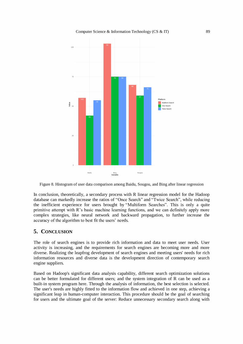
Computer Science & Information Technology (CS & IT) 89
55
42
103
57
75
68
75 66
59
0
25
50
75
100
Baidu Bing Sougou
Variable
Valu
e
Platform
Multiform Search
One Search
Twice Search
Figure 8. Histogram of user data comparison among Baidu, Sougou, and Bing after linear regression
In conclusion, theoretically, a secondary process with R linear regression model for the Hadoop database can markedly increase the ratios of “Once Search” and “Twice Search”, while reducing the inefficient experience for users brought by “Multiform Searches”. This is only a quite primitive attempt with R’s basic machine learning functions, and we can definitely apply more complex strategies, like neural network and backward propagation, to further increase the
accuracy of the algorithm to best fit the users’ needs.
5. CONCLUSION
The role of search engines is to provide rich information and data to meet user needs. User activity is increasing, and the requirements for search engines are becoming more and more diverse. Realizing the leapfrog development of search engines and meeting users' needs for rich information resources and diverse data is the development direction of contemporary search engine suppliers. Based on Hadoop's significant data analysis capability, different search optimization solutions
can be better formulated for different users; and the system integration of R can be used as a built-in system program here. Through the analysis of information, the best selection is selected. The user's needs are highly fitted to the information flow and achieved in one step, achieving a significant leap in human-computer interaction. This procedure should be the goal of searching for users and the ultimate goal of the server: Reduce unnecessary secondary search along with

90 Computer Science & Information Technology (CS & IT)
multi-form search and use the most straightforward operation to achieve the most valuable information aggregation. The current paper only proves the market value and uses the value of using R to improve search
efficiency from the user's point of view. This new algorithm is achieved through the combination of Hadoop and R. With a personalized regression analysis for individual users, the search engine might achieve an optimized resources integration and significantly reduce the number of the secondary and multi-form searches. To realize this new algorithm, this article also provides a program frame for its analysis procedures. However, this proposal has not been fully verified, nor has it been tested. In this paper, R is not discussed in detail, and the cited demonstration data are not rigorous enough, the data sampling is not comprehensive, and the age and gender of users are not limited. This issue is the shortcoming of this paper, which needs further investigation.
REFERENCES
[1] Stéphane Dray, Anne B. Dufour, and Daniel Chessel, (2007)”The ade4 package—II”, Two-table and
K-table methods. R News, 7(2), pp47—52.
[2] Friedrich Leisch, (2007) Review of “The R Book”. R News, 7(2), pp53—54.
[3] Hee-Seok Oh and Donghoh Kim, (2007) SpherWave: An R package for analyzing scattered spherical
databy spherical wavelets. R News, 7(3), pp2--7.
[4] Guido Schwarzer, (2007)meta: An R package for meta-analysis. R News, 7(3), pp40—45.
[5] Sebastián P. Luque, (2007) Diving behaviour analysis in R. R News, 7(3), pp8--14.
[6] John Fox, (2007)Extending the R Commander by “plug-in” packages. R News, 7(3), pp46--52.
[7] White, Tom, (2012)Hadoop: The Definitive Guide, O'rlly Media Inc Gravenstn Highway North, 215(11), pp1 - 4.
[8] Taylor R C, (2010)An overview of the Hadoop/MapReduce/HBase framework and its current
applications in bioinformatics, Bmc Bioinformatics, Suppl 12(S12): S1.
[9] A A O, B J D, B R D S, (2013)'Big data', Hadoop and cloud computing in genomics, Journal of
Biomedical Informatics, 46(5), pp774-781.
[10] Robin K. S. Hankin, (2007) Very large numbers in R: Introducing package Brobdingnag. R News,
7(3), pp15--16.
[11] Robert J Knell, (2013) Introductory R: A Beginner's Guide to Data Visualisation and Analysis using
R.pp3--8
[12] Alejandro Jara, (2007)Applied bayesian non- and semi-parametric inference usingDPpackage. R
News, 7(3), pp17--26.
[13] Sanford Weisberg and Hadley Wickham, (2007)Need a hint? R News, 7(3), pp36--38.
[14] John Verzani, (2007)An introduction to gWidgets. R News, 7(3), pp26--33.
[15] Patrick Mair and Reinhold Hatzinger, (2007)Psychometrics task view. R News, 7(3), pp38—40.
[16] Diego Kuonen and Reinhard Furrer, (2007)Data mining avec R dans un monde libre. Flash
Informatique Spécial Été, pp45—50.
[17] Morandat, F. , Hill, B. , Osvald, L. , & Vitek, J. . (2012). Evaluating the design of the R language. Proceedings of the 26th European conference on Object-Oriented Programming. Springer-Verlag.
[18] Wang, G. , Xu, Y. , Duan, Q. , Zhang, M. , & Xu, B. . (2017). Prediction model of glutamic acid
production of data mining based on R language. 2017 29th Chinese Control And Decision Conference
(CCDC). IEEE.
[19] Bill Alpert, (2007)Financial journalism with R. R News, 7(3), pp34--36.
[20] Abouzeid A, Bajda-Pawlikowski K, Abadi D J, et al, (2009)HadoopDB: An Architectural Hybrid of
MapReduce and DBMS Technologies for Analytical Workloads, Proc. VLDB Endowment, 2(1),
pp922-933.
[21] Thusoo A, Sarma J S, Jain N, et al, (2010)Hive - a petabyte scale data warehouse using Hadoop.

Computer Science & Information Technology (CS & IT) 91
AUTHOR
I am a fourth-year student in University of California, Los Angeles. I double-major in
Economics and Statistics, with a minor in Mathematics. For my internships, I used to
work as a high-frequency trader in Citadel Securities, Chicago, IL, and an executive
director assistant in J P Morgan, London, UK. I also worked as a research assistant in
Institute of Computing Technology, Chinese Academy of Science, for Distributed
Computing System, Big Data, Architecture and Machine Learning.
© 2020 By AIRCC Publishing Corporation. This article is published under the Creative Commons
Attribution (CC BY) license.

92 Computer Science & Information Technology (CS & IT)

David C. Wyld et al. (Eds): COMIT, SIPO, AISCA, MLIOB, BDHI - 2020
pp. 93-98, 2020. CS & IT - CSCP 2020 DOI: 10.5121/csit.2020.101608
EXTRACTING THE SIGNIFICANT DEGREES OF
ATTRIBUTES IN UNLABELED DATA USING
UNSUPERVISED MACHINE LEARNING
Byoung Jik Lee
School of Computer Sciences, Western Illinois University
Macomb, IL, U.S.A.
ABSTRACT We propose a valid approach to find the degree of important attributes in unlabeled dataset to
improve the clustering performance. The significant degrees of attributes are extracted through
the training of unsupervised simple competitive learning with the raw unlabeled data. These
significant degrees are applied to the original dataset and generate the weighted dataset
reflected by the degrees of influentialvalues for the set ofattributes. This work is simulated on
the UCI Machine Learning repository dataset. The Scikit-learn K-Means clustering with raw
data, scaled data, and the weighted data are tested. The result shows that the proposed
approach improves the performance.
KEYWORDS Unsupervised MachineLearning, Simple Competitive Learning, SignificantDegree of Attributes,
Scikit-learn K-Means Clustering, Weighted Data, UCI Machine Learning Data.
1. INTRODUCTION
Data is extremely valuable to our lives. Data are being collected and saved almost anywhere and anytime. The size of data is increasing exponentially over time. Especially, the data that comes
without a label, unlabeled data, is growing in greater volume and at a faster rate than labeled data.
The unlabeled data is essential for unsupervised machine learning. Unsupervised learning with
unlabeled dataset has a limited scale of computation and performance compared to supervised learning with labelled dataset. However, clustering, a process of partitioning a given data set into
distinct groups, has been applied to the varieties of data mining, knowledge discovery, and
pattern recognition applications [1] [2].
To enable data to be used for machine learning, some steps of data preprocessing are required
such as data cleaning, data integration, data reduction, and data transformation [3].Normalization
is a one of the most popular methods in data preprocessing. Attributes values are typically normalized by scaling original data within the specified range of values. When the range of the
attribute values are significantly varied, normalization process has been used to balance the
importance of the attributes of the data.
However, if some attributes have significant impacts on data clustering, it is advisable to treat
these important attributes as meaningful core properties for clustering. There are two approaches to deal with the set of attributes. One method is to construct new attributes by adding new
attributes or replacing current attributes from existing attributes. The other method is to deduct

94 Computer Science & Information Technology (CS & IT)
the irrelevant or redundant attributes [4][5][6]. Both methods change the set of existing attributes by increasing or decreasing the set of attributes. This can lead to additional inconsistency issues
when new data are added in the future.
In this paper, to improve the clustering performance, we propose a method of assigning significant degree to important attribute sets while maintaining the set of attributes. In section 2,
unsupervised simple competitive learning [7][8] is used to extract the estimated significant
degree for each attribute, Sj, from the result of training with unlabeled data. This significant degree, Sj, is applied to the original dataset and produces the weighted dataset.
To verify this proposed method, K-means clustering, one of the most widely used method because of its simplicity to use and its high efficiency of computation, is employed. K-means
clustering has been successfully applied to the variety of applications [9]. In section 3, the K-
Means imports the trained weighted dataset and tests the popular data set. The result of Iris,
Seeds, and Wine dataset of UCI Machine Learning Repository [10] shows that the proposed approach improves the performance.
2. SYSTEM ARCHITECTURE This system has two modules. In Module 1, unsupervised simple competitive learning trains the
raw unlabeled data and produces the estimated significant degree for each attribute, Sj. In Module
2, the K-Means clustering with raw data, scaled data, and the weighted data by the significant
degrees are tested.
2.1. Module 1: Finding out the significant attributes by Simple Competitive
Learning
Figure 1 shows the architecture of Simple Competitive Learning. The unlabeled data with j number of attributes are fed into the same number of input units in the network. The number of
output units, i, is the number of clustering groups. The winner is the output unit with the largest
net input for the feeding input vector X. The solid line represents an excitatory connection and the dashed line which connects output unit each other represents an inhibitory connection.
Figure 1. Simple Competitive Learning Network
With the given unlabeled dataset, the Simple Competitive Learning model is trained based on the
learning algorithm (1) followed by the normalization process to avoid no bounds on the weight.
Wji(t+1) = Wji(t) + n (Xj
u – Wji(t)) , (1)

Computer Science & Information Technology (CS & IT) 95
Where n is the learning rate, u is the uth training data, t is the time step.When the training is completed, the weight Wji represents the strength weight between the attribute j and the clustering
group i. The significant degree of each attribute jis computed from the equation (2).
Sj = ∑I Wji (2)
The significant vector S constitutes the significant degree of each attribute Sj, S = (S1, S2, …,
Sj).The significant degree of each attribute, Sj, is applied to the unlabeled dataset, Xju, and
produces the weighted data, Weighted_dataju, which embedded the significant degree of attribute
j.
Weighted_dataj
u = Xju × Sj, (3)
Where j is the corresponding attribute, u is the uth training data.
2.2. Module 2: K-Means clustering with raw data, scaled data, and weighted data We used the Scikit-learn library [11] to explore K-Means clustering performance with the raw
data, scaled data, and the proposed weighted data. Figure 2 illustrates the procedure of the
system. The popular Elbow method of Scikit-learn library [11] was used to decide the number of
clusters of the Simple Competitive learning Module 1.
Input: Unlabeled dataset
Output: Significant degree of each attributej, Sj 0. Decide the number of clusters by Elbow method
1. Feed the unlabeled data into Simple Competitive Learning Network
2. Train the Simple Competitive Learning network based on the learning equation (1) 3. Compute the Significant degree of each attributes, Sj, by equation (2)
4. Apply the Significant degree to the unlabeled data to produce the Weighted data by
equation (3).
5. Explore K-Means clustering with raw data, scaled data, and the proposed weighted data.
Figure 2. Exploring the Significant Degree of Attributes Procedure
3. EXPERIMENT RESULT
3.1. The Dataset and the Significant Degree of the Data
UCI Machine Learning repository dataset was used for performance evaluation. Wine dataset,
Iris dataset, and Seed datasets are accessed to verify the effect of the proposed approach. The Iris
data has 150 instances, four attributes (length and width of sepals and petals), and three classes. Each class (Iris setosa, Iris virginica, and Iris versicolor) has 50 instances. The input values of the
attributes are in centimeters. Wine data has 13 attributes (Alcohol, Malic acid, Ash, Alcalinity of
ash, Magnesium, Total phenols, Flavanoids, Nonflavanoid phenols, Proanthocyanins, Color intensity, Hue, OD280/OD315 of diluted wines and Proline), 178 instances, and 3 classes. The
input values of attributes are continuous. The Seed data has seven attributes (area A, perimeter P,
compactness C, length of kernel, width of kernel, asymmetry coefficient, length of kernel groove), 210 instances, and 3 classes. The input values of all attributes are real-valued
continuous.

96 Computer Science & Information Technology (CS & IT)
As shown in Figure 3, three attributes (compactness C, asymmetry coefficient, length of kernel groove) of See data are the significant attributes for determining the clustering. The significant
degree for Seed data is [0.3103793337657787, 0.38404893997441847, 0.5627959563346043,
0.38879262126954195, 0.35041866849291087, 0.5255126477711352, 0.47805183239161064].
Figure 3. The significant degree of Seed data
As shown in Figure 4, the last attribute (petal width in cm) of Iris data influenced to decide the clustering.The significant degree for Iris data is [0.7569583177646524, 0.6202633420788992,
0.7613989085834454, 1.1575052380511397].
Figure 4. The significant degree of Iris data
The significant degree for Wine data is [0.49679553839142865, 0.4253067347939007,
0.3365439062186957, 0.2845606505403928, 0.1526467495303905, 0.2809781772430352, 0.2718178595519532, 0.20136617303733317, 0.27474333797269745, 0.13341331581839957,

Computer Science & Information Technology (CS & IT) 97
0.25327013905125795, 0.37015396979853094, 0.20009014838009148]. As shown in Figure 5, the first attribute (Alcohol) and the second attribute (Malic acid) of Wine data significantly
contributes to determining three types of wine.
3.2. Improvements and Limitations
Table 1 and Table 2 show that the proposed approach improves the performance of clustering problem in three datasets. Comparing the scaled data with the suggested weight data, the
performance of the Iris and Seed data are improved by 4.7% and 3.4%, respectively. Of the three
problems (Wine, Iris, Seed), the proposed approach is the most effective in the Iris problem,
because one attribute (petal width in cm) has a high significant degree than other attributes. As observed in 1.7% improvement of Wine data, this approach has limitations if there are not
significant attributes in the data.
Figure 5. The significant degree of Wine data
Table 1. Performance of raw data, scaled data, weighted data
Models Correction rate
Wine Iris Seeds
Raw data 71.3% 89.3% 89.5%
Scaled data 95.5% 89.3% 89%
Weighted data 97.2% 94.0% 92.4%
Scaled data to Weighted data 1.7% 4.7% 3.4%

98 Computer Science & Information Technology (CS & IT)
Table 2. Performance of raw data, scaled data, weighted data
Wine Seeds Iris
A B C A B C A B C
Raw data A 46 0 13 60 1 9 50 0 0
B 1 51 19 10 60 0 0 48 2
C 0 18 30 2 0 68 0 14 36
Scaled
data
A 59 0 0 58 2 10 50 0 0
B 2 63 6 8 68 0 0 48 2
C 0 0 48 3 0 67 0 14 36
Weighted
data
A 58 0 1 64 2 4 50 0 0
B 2 67 2 3 67 0 0 45 5
C 0 1 47 7 0 63 0 4 46
4. CONCLUSIONS
This paper proposes an approach to extract the significant degree of each attribute in unlabeled
dataset for efficient clustering performance while maintaining the set of attributes.This significant degree of each attribute converts the unlabeled raw data into the weighted data which reflects the
importance of each attribute. This approach is tested by Scikit-learn K-Means clustering on some
of UCI Machine Learning repository dataset with raw data, scaled data, and weighted data. The result shows that the proposed approach improves the performance for all tested data sets.
REFERENCES [1] U.M. Fayyad, G. Piatetsky-Shapiro, P. Smyth, and R. Uthurusamy, Advances in KnowledgeDiscovery
and Data Mining. AAAI/MIT Press, 1996
[2] R.O. Duda and P.E. Hart, Pattern Classification and Scene Analysis. New York: John Wiley & Sons,
1973
[3] J. Han, M. Kamber, and J. Pei, Data Mining: Concepts and Techniques, 3rd ed., Morgan Kaufmann,
2012
[4] H. Liu and H. Motoda. Feature Selection for Knowledge Discovery and Data Mining. Kluwer
Academic, 1998.
[5] W. Siedlecki and J. Sklansky. On automatic feature selection. Int. J. Pattern Recognition and Artificial
Intelligence, 2:197–220, 1988.
[6] Pyle, D., 1999. Data Preparation for Data Mining. Morgan Kaufmann Publishers, Los Altos,
California. [7] J. Hertz, A. Krogh, R. Palme, Introduction to the Theory of Neural Computation, Addison Wesley,
1991
[8] D. E. Rumelhart and J. L. McClelland, Parallel Distributed Processing, MIT Press, 1986,, pp. 151-193
[9] M M. N. Murty, A. K. Jain and P. J. Flynn, “Data Clustering: A Review”, ACM Computing Survey,
Vol. 31, No. 3, 1999, pp 264-323.
[10] D. J. Newman, S. Hettich, C.L. Blake, C.J. Merz, UCI repository of machine learning databases,
Department of Information and Computer Science, University of California, Irvine, CA, 1988
[11] S. Rashika and V. Mirjalili, Python Machine Learning. 2nd Edition. Birmingham, UK: Packt
Publishing, 2017
© 2020 By AIRCC Publishing Corporation. This article is published under the Creative Commons
Attribution (CC BY) license.
David C. Wyld et al. (Eds): COMIT, SIPO, AISCA, MLIOB, BDHI - 2020
pp. 99-108, 2020. CS & IT - CSCP 2020 DOI: 10.5121/csit.2020.101609
A PREDICTIVE MODEL FOR KIDNEY
TRANSPLANT GRAFT SURVIVAL USING
MACHINE LEARNING
Eric S. Pahl1, W. Nick Street2, Hans J. Johnson3 and Alan I. Reed4
1Health Informatics, University of Iowa, Iowa, USA 2Management Sciences, University of Iowa, Iowa, USA
3Electrical and Computer Engineering, University of Iowa, Iowa, USA 4Organ Transplant Centre, University of Iowa, Iowa, USA
ABSTRACT Kidney transplantation is the best treatment for end-stage renal failure patients. The
predominant method used for kidney quality assessment is the Cox regression-based,
kidney donor risk index. A machine learning method may provide improved prediction of
transplant outcomes and help decision-making. A popular tree-based machine learning
method, random forest, was trained and evaluated with the same data originally used to
develop the risk index (70,242 observations from 1995-2005). The random forest
successfully predicted an additional 2,148 transplants than the risk index with equal type II
error rates of 10%. Predicted results were analyzed with follow-up survival outcomes up to 240 months after transplant using Kaplan-Meier analysis and confirmed that the random
forest performed significantly better than the risk index (p<0.05). The random forest
predicted significantly more successful and longer-surviving transplants than the risk
index. Random forests and other machine learning models may improve transplant
decisions.
KEYWORDS Kidney Transplant, Decision Support, Random Forest, Health Informatics, Clinical
Decision Making, Machine Learning & Survival Analysis
1. INTRODUCTION
There is little research into the methodology regarding how organ transplant stakeholders make
decisions, predictions, and assessments of viability and matching for deceased donor kidney transplantation at the time of organ offer and acceptance. Clinical decisions have traditionally
relied on the time-tested orthodoxy of data derived from Cox regression-based models to provide
statistical relevance to decision making. Recent advances in machine learning (ML) methods provide the opportunity to create highly nonlinear models with complex interactions among
variables that may provide superior predictive power. Machine learning usage in medical
domains is increasing as demonstrated by successful applications for predicting better utilization of perioperative antibiotics, predicting hospital lengths of stay, and indeed even recently in
formulating alternative models for organ distribution and post-transplant implied utilization [1-5].
Despite evidence-based clinical and cost advantages of transplantation, nearly 1 in 5 viable
deceased-donor kidneys procured are discarded (~4,000 per year) [6]. Many studies have demonstrated a significant survival benefit for wait-listed patients to accept (or for centers to
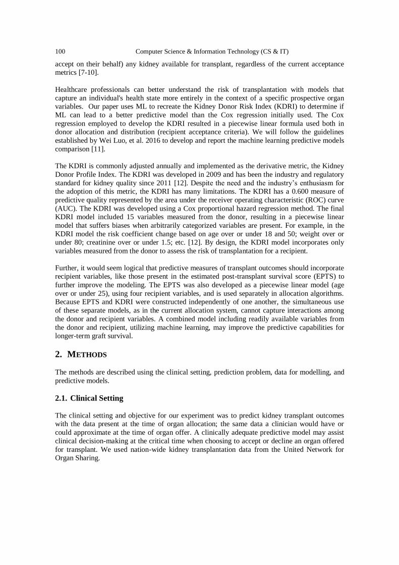
100 Computer Science & Information Technology (CS & IT)
accept on their behalf) any kidney available for transplant, regardless of the current acceptance metrics [7-10].
Healthcare professionals can better understand the risk of transplantation with models that
capture an individual's health state more entirely in the context of a specific prospective organ variables. Our paper uses ML to recreate the Kidney Donor Risk Index (KDRI) to determine if
ML can lead to a better predictive model than the Cox regression initially used. The Cox
regression employed to develop the KDRI resulted in a piecewise linear formula used both in donor allocation and distribution (recipient acceptance criteria). We will follow the guidelines
established by Wei Luo, et al. 2016 to develop and report the machine learning predictive models
comparison [11].
The KDRI is commonly adjusted annually and implemented as the derivative metric, the Kidney
Donor Profile Index. The KDRI was developed in 2009 and has been the industry and regulatory
standard for kidney quality since 2011 [12]. Despite the need and the industry’s enthusiasm for the adoption of this metric, the KDRI has many limitations. The KDRI has a 0.600 measure of
predictive quality represented by the area under the receiver operating characteristic (ROC) curve
(AUC). The KDRI was developed using a Cox proportional hazard regression method. The final KDRI model included 15 variables measured from the donor, resulting in a piecewise linear
model that suffers biases when arbitrarily categorized variables are present. For example, in the
KDRI model the risk coefficient change based on age over or under 18 and 50; weight over or under 80; creatinine over or under 1.5; etc. [12]. By design, the KDRI model incorporates only
variables measured from the donor to assess the risk of transplantation for a recipient.
Further, it would seem logical that predictive measures of transplant outcomes should incorporate recipient variables, like those present in the estimated post-transplant survival score (EPTS) to
further improve the modeling. The EPTS was also developed as a piecewise linear model (age
over or under 25), using four recipient variables, and is used separately in allocation algorithms. Because EPTS and KDRI were constructed independently of one another, the simultaneous use
of these separate models, as in the current allocation system, cannot capture interactions among
the donor and recipient variables. A combined model including readily available variables from
the donor and recipient, utilizing machine learning, may improve the predictive capabilities for longer-term graft survival.
2. METHODS The methods are described using the clinical setting, prediction problem, data for modelling, and
predictive models.
2.1. Clinical Setting
The clinical setting and objective for our experiment was to predict kidney transplant outcomes with the data present at the time of organ allocation; the same data a clinician would have or
could approximate at the time of organ offer. A clinically adequate predictive model may assist
clinical decision-making at the critical time when choosing to accept or decline an organ offered
for transplant. We used nation-wide kidney transplantation data from the United Network for Organ Sharing.

Computer Science & Information Technology (CS & IT) 101
2.2. Prediction Problem
The prediction problem was the classification of retrospective data with three prognostic binary
outcomes: graft failure at 12, 24, and 36 months after transplant were abbreviated as GF12, GF24, and GF36 respectively. The positive (+) outcome for GF12 meant that we observed graft
loss within 12 months after transplant and the negative (-) outcome for GF12 meant that graft had
not failed at 12-month follow-up. A false positive (type I error) in prediction of graft failure may lead to a declined kidney that would have been successful (missed opportunity). A false negative
(type II error) may lead to an accepted kidney that failed within the follow-up period. For this
experiment, we highlighted and compared all predictive models’ performance at 10% false
negative rate because the overall observed graft failure rate is 10% at 12 months follow up. Models with more predicted negative GF outcomes were able to achieve higher utility of
available kidneys without increasing risk to patients. We validated the performance of our models
using 10-fold cross-validation, whereby we blinded the models to 10% held-out data for testing and reported the test performance only [13].
Table 1 contains descriptions and definitions of predictions; true positive (TP), true negative (TN), false positive (FP), and false negative (FN). The models’ predictions are labeled “Predicted
GF” and the observed transplant outcomes are “Actual GF.” When the Predicted GF and Actual
GF are the same, the model predicted correctly. There are two types of model prediction errors;
False Positives (Type I errors) happen when a model predicts that the graft would fail but the observed data show success, this is a missed opportunity; False Negatives (Type II errors) happen
when a model predicts that the graft would survive but the observed data show failure. False
Negatives are the worst prediction errors from a clinical perspective; predicting a success, transplanting, and the graft failing or patient dying.
Table 1. Definitions of prediction outcomes when models were used to predict graft failure (GF) within the
months following a kidney transplant.
Confusion Matrix Predicted GF Actual GF Description
True Positive Failed (1) Failed (1) Model Correctly Predicted a Bad
Kidney (avoided a bad kidney, bigger is better)
True Negative Not Failed (0) Not Failed
(0)
Model Correctly Predicted a Good
Kidney
(bigger is better)
False Positive (type
I error)
Failed (1) Not Failed
(0)
Model Error Missed a Good Kidney
(missed opportunity, smaller is better)
False Negative (type
II error)
Not Failed (0) Failed (1) Model Error Missed a Bad Kidney
(graft failure, smaller is better)
2.3. Data for Modelling
We reconstructed, as closely as possible, the original data set used by Rao for the development of KDRI [12]. First, we obtained Standard Transplant Analysis and Research data inclusive of
September 29, 1987, through March 31, 2016. The data were filtered by transplantation date
within the acceptable date range (01/01/1995 to 12/31/2005) and only included deceased donor
kidneys, Initial Data ni, (see data reduction in the first row of Table 2). Excluded in sequence from the analysis were: recipients aged less than 18 years, recipients with a previous transplant,
multi-organ transplant recipients, and ABO-incompatible patients, keeping consistent with Rao.
We also removed observations with invalid and/or missing data: donor height (<50cm, >213cm), weight (<10kg, >175kg), and creatinine (<0.1mg/dL, >8.0mg/dL). Finally, we removed

102 Computer Science & Information Technology (CS & IT)
observations without a valid entry for the KDRI_RAO variable. Table 2 compares the number of removed observations from Rao’s study and our study for each missing or invalid variable [12].
Table 2. Observed preprocessing of the UNOS STAR data compared to KDRI development data from
kidney transplants 1995-2005.
Removed Observations KDRI Observed
Initial Data 92102 91996
Pediatric Transplants 3733 3724
Previous Transplants 13122 12390
Multi-Organ Transplants 1556 1850
ABO Incompatible Transplants 211 176
Invalid/Missing Donor Height 2481 1009
Invalid/Missing Donor Weight 667
Invalid/Missing Donor Creatinine 892 949
Without “KDRI_RAO” 0 1181
Final Study Sample 69440 70242
The predictor variables were the same as the ones present in KDRI and EPTS. Donor variables
were those used in the final model of KDRI: age, race, history of hypertension, history of diabetes, serum creatinine, cerebrovascular cause of death, height, weight, donation after cardiac
death, hepatitis C virus status, HLA-B and HLA-DR mismatching, en-bloc transplant, and double
kidney transplant indicators (two for one), and known cold ischemia time at time of offer. Transplant recipient variables from EPTS score were used in our MLM; recipient age, diabetes,
and time on dialysis - notably excluding recipients with prior transplant and multiorgan
transplants based on the filter criteria.
We evaluated the predictive performance of the models with an industry standard 10-fold cross-
validation approach [13]. The completion of the cross-validation process yielded a ranked list of
predicted transplant outcome probabilities. In 10-fold cross-validation, the models are evaluated on external test data that are never used in training. We evaluated the models, using the predicted
ranked lists, by generating the ROC curve and calculating the AUC as standard measures of
predictive quality and analyzed the confusion matrices with false negative rates at 10%. Additionally, performed Kaplan-Meier survival analysis with survival groups selected by
prediction cut-off at a 10% false negative rate.
2.4. Predictive Models
In contrast to Rao’s Cox proportional hazard regression method, we explored a supervised random forest (RF) ML classification model. The RF algorithm constructs and combines the
predictions of thousands of machine-generated decision trees to model the probability of graft
failure [14]. The algorithm created each decision tree using a subset of the training data called a
bootstrap sample. Each bootstrap sample is balanced by under sampling the majority outcome cases (negatives) such that the resulting ratio was 1:1. Each tree consists of multiple decision
nodes constructed by randomly selecting a subset of the predictive variables and choosing the one
that maximizes the Gini index, a measure of information gained from the use of each variable. Training continued until “exhaustion”: each tree completely fits the training sample. When
classifying new examples, all the trees made a prediction, and the output of the RF was the
percentage of votes for each outcome, one vote per tree, and the predicted outcome was assigned based on majority vote.

Computer Science & Information Technology (CS & IT) 103
The choice of the RF algorithm allowed for mixed data types (binary, categorical, and numerical) without scaling or significant data modification. The RF training is computationally efficient, is
robust to outliers and co-linearities, contains simple tuning parameters, and has demonstrated
success for a variety of healthcare data applications [14, 15]. RFs have also demonstrated utility
in predicting deceased donor organ transplantation success and offer acceptances in simulated organ allocation models [3, 4].
The contribution of each tree in an RF was similar to getting thousands of opinions based on a professional colleague's background. The clinical implementation of the RF algorithm worked
similarly to secondary and tertiary opinions among professionals across the country convening
for the treatment of a complicated case. A random subset of all available variables and clinical observations informed the construction of every decision tree and resulted in a unique perspective
represented by each tree. The majority vote among the decision trees, was the final prediction of
graft failure. The three models tested were: RF using only donor variables from KDRI (RFD), RF
using donor variables from KDRI and recipient variables from EPTS (RFDR), and Rao’s KDRI. Figure 1 demonstrates the different numbers of trees used for RFD and RFDR models including
stratifying and balancing to obtain BSS and the resulting AUC. Increasing the number of trees
improved the AUC reached by RFD and RFDR, and both converged between 1000 and 1500 trees. The number of trees was a significant hyperparameter for the RF algorithm. KDRI results
do not depend on the number of trees.
500 1000 1500
0.5
90.6
00
.61
0.6
20.6
30
.64
0.6
5
Models' AUC for given GF
Number of Trees
Cro
ss−
Va
lidate
d A
UC
●
● ● ● ●
●
●● ● ●
● ●
KDRI GF12KDRI GF24KDRI GF36
RFD GF12RFD GF24RFD GF36
RFDR GF12RFDR GF24RFDR GF36
Figure 1. AUC for RF models created with different numbers of trees. KDRI model’s AUC performance
does not depend on the number of trees.
3. RESULTS
RFDR performed better than RFD in all scenarios: adding recipient variables improved the predictive quality of the RFDR model. This is particularly true when predicting longer graft
survival outcomes where RFDR performed increasingly better with longer time periods; GF12
(AUC = 0.636), GF24 (AUC = 0.638), GF36 (AUC = 0.644). RFD and KDRI, both models built without recipient variables, did not predict as well as the RFDR model did at the longer graft
outcomes.
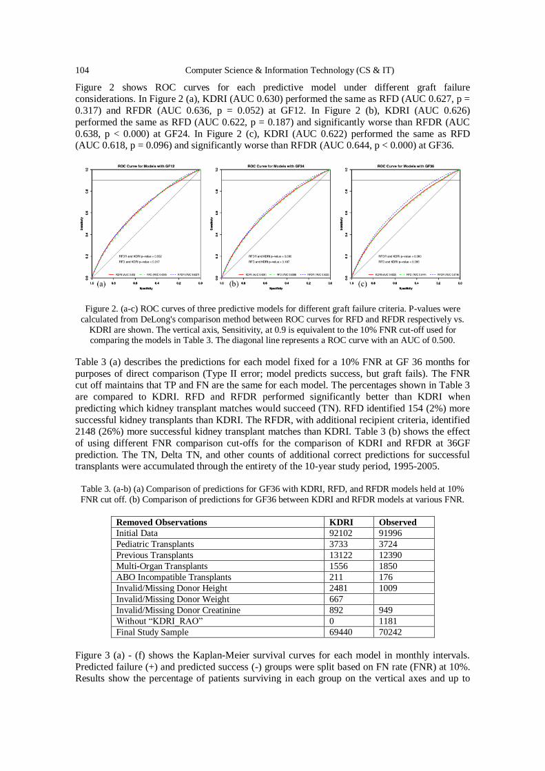
104 Computer Science & Information Technology (CS & IT)
Figure 2 shows ROC curves for each predictive model under different graft failure considerations. In Figure 2 (a), KDRI (AUC 0.630) performed the same as RFD (AUC 0.627, p =
0.317) and RFDR (AUC 0.636, p = 0.052) at GF12. In Figure 2 (b), KDRI (AUC 0.626)
performed the same as RFD (AUC 0.622, p = 0.187) and significantly worse than RFDR (AUC
0.638, p < 0.000) at GF24. In Figure 2 (c), KDRI (AUC 0.622) performed the same as RFD (AUC 0.618, p = 0.096) and significantly worse than RFDR (AUC 0.644, p < 0.000) at GF36.
Figure 2. (a-c) ROC curves of three predictive models for different graft failure criteria. P-values were
calculated from DeLong's comparison method between ROC curves for RFD and RFDR respectively vs.
KDRI are shown. The vertical axis, Sensitivity, at 0.9 is equivalent to the 10% FNR cut-off used for comparing the models in Table 3. The diagonal line represents a ROC curve with an AUC of 0.500.
Table 3 (a) describes the predictions for each model fixed for a 10% FNR at GF 36 months for
purposes of direct comparison (Type II error; model predicts success, but graft fails). The FNR cut off maintains that TP and FN are the same for each model. The percentages shown in Table 3
are compared to KDRI. RFD and RFDR performed significantly better than KDRI when
predicting which kidney transplant matches would succeed (TN). RFD identified 154 (2%) more
successful kidney transplants than KDRI. The RFDR, with additional recipient criteria, identified 2148 (26%) more successful kidney transplant matches than KDRI. Table 3 (b) shows the effect
of using different FNR comparison cut-offs for the comparison of KDRI and RFDR at 36GF
prediction. The TN, Delta TN, and other counts of additional correct predictions for successful transplants were accumulated through the entirety of the 10-year study period, 1995-2005.
Table 3. (a-b) (a) Comparison of predictions for GF36 with KDRI, RFD, and RFDR models held at 10%
FNR cut off. (b) Comparison of predictions for GF36 between KDRI and RFDR models at various FNR.
Removed Observations KDRI Observed
Initial Data 92102 91996
Pediatric Transplants 3733 3724
Previous Transplants 13122 12390
Multi-Organ Transplants 1556 1850
ABO Incompatible Transplants 211 176
Invalid/Missing Donor Height 2481 1009
Invalid/Missing Donor Weight 667
Invalid/Missing Donor Creatinine 892 949
Without “KDRI_RAO” 0 1181
Final Study Sample 69440 70242
Figure 3 (a) - (f) shows the Kaplan-Meier survival curves for each model in monthly intervals.
Predicted failure (+) and predicted success (-) groups were split based on FN rate (FNR) at 10%. Results show the percentage of patients surviving in each group on the vertical axes and up to
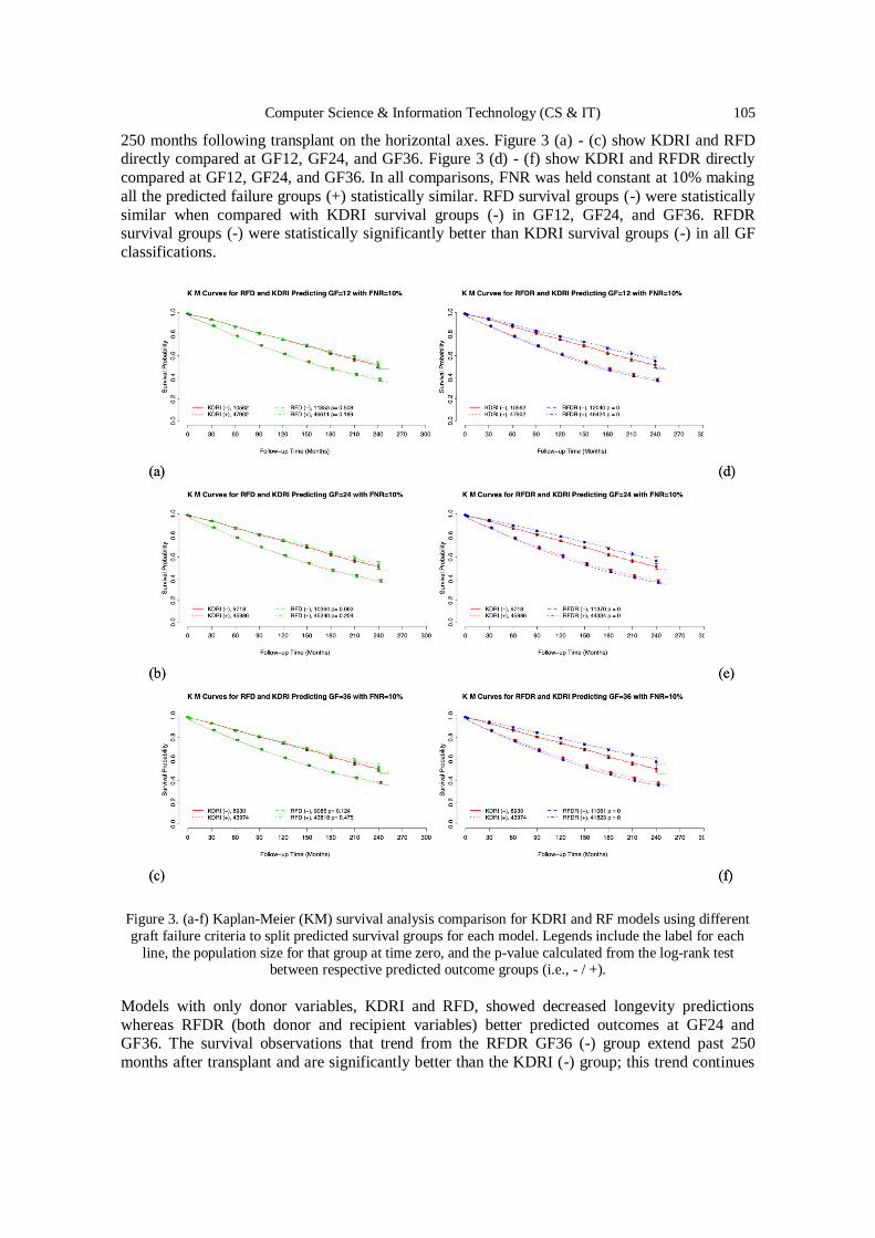
Computer Science & Information Technology (CS & IT) 105
250 months following transplant on the horizontal axes. Figure 3 (a) - (c) show KDRI and RFD directly compared at GF12, GF24, and GF36. Figure 3 (d) - (f) show KDRI and RFDR directly
compared at GF12, GF24, and GF36. In all comparisons, FNR was held constant at 10% making
all the predicted failure groups (+) statistically similar. RFD survival groups (-) were statistically
similar when compared with KDRI survival groups (-) in GF12, GF24, and GF36. RFDR survival groups (-) were statistically significantly better than KDRI survival groups (-) in all GF
classifications.
Figure 3. (a-f) Kaplan-Meier (KM) survival analysis comparison for KDRI and RF models using different
graft failure criteria to split predicted survival groups for each model. Legends include the label for each
line, the population size for that group at time zero, and the p-value calculated from the log-rank test between respective predicted outcome groups (i.e., - / +).
Models with only donor variables, KDRI and RFD, showed decreased longevity predictions
whereas RFDR (both donor and recipient variables) better predicted outcomes at GF24 and GF36. The survival observations that trend from the RFDR GF36 (-) group extend past 250
months after transplant and are significantly better than the KDRI (-) group; this trend continues
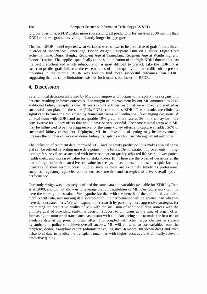
106 Computer Science & Information Technology (CS & IT)
to grow over time. RFDR makes more successful graft predictions for survival at 36 months than KDRI and these grafts survive significantly longer in aggregate.
The final RFDR model reported what variables were shown to be predictive of graft failure, listed
in order of importance; Donor Age, Donor Weight, Recipient Time on Dialysis, Organ Cold Ischemia Time, Donor Height, Recipient Age at Transplant, Recipient Age at Waitlisting, and
Donor Creatine. This applies specifically to the subpopulation of the high-KDRI donors that has
the best prediction and which subpopulation is most difficult to predict. Like the KDRI, it is easier to predict graft failure at the extreme ends of donor quality and more difficult to predict
outcomes in the middle. RFDR was able to find more successful outcomes than KDRI,
suggesting that the same limitations exist for both models but lesser for RFDR.
4. DISCUSSION
Safer clinical decisions informed by ML could empower clinicians to transplant more organs into
patients resulting in better outcomes. The margin of improvement by our ML amounted to 2148 additional kidney transplants over 10 years (about 200 per year) that were correctly classified as
successful transplants at the same (10% FNR) error rate as KDRI. These results are clinically
significant because the tools used by transplant teams will influence life-changing decisions. A clinical team with KDRI and an acceptable 10% graft failure rate at 36 months may be more
conservative for kidney offers that would have been successful. The same clinical team with ML
may be influenced to be more aggressive for the same kidney offers and capture an added 26% of
successful kidney transplants. Deploying ML in a live clinical setting may be an avenue to increase the number of deceased donor kidney transplants without sacrificing patient outcomes.
The inclusion of recipient data improved AUC and longevity prediction; this makes clinical sense and can be refined by adding more data points in the future. Demonstrated improvements in long-
term graft survival are associated with increased patient quality-adjusted life years, lower patient
health costs, and increased value for all stakeholders [8]. These are the types of decisions at the time of organ offer that can drive real value for the system as opposed to those that optimize only
measures of short term success. Studies such as these are extremely timely as professional
societies, regulatory agencies and others seek metrics and strategies to drive overall system
performance.
Our study design was purposely confined the same data and variables available for KDRI by Rao,
et al. 2009, and did not allow us to leverage the full capabilities of ML. Our future work will not have these design constraints. We hypothesize that with the benefit of the additional variables,
more recent data, and missing data interpolation, the performance will be greater than what we
have demonstrated here. We will expand this research by pursuing more aggressive strategies for
optimizing the predictive quality of ML with the inclusion of additional data sources with the ultimate goal of providing real-time decision support to clinicians at the time of organ offer.
Increasing the number of transplants has to start with clinicians being able to make the best use of
available data at the point of organ offer. This coupled with other larger changes in system dynamics and policy to achieve overall success. ML will allow us to use variables from the
recipient, donor, transplant center (administrative, logistical-temporal turndown data) and even
behavioral data to predict the transplant outcomes with higher accuracy and clinically relevant predictive quality.

Computer Science & Information Technology (CS & IT) 107
ACKNOWLEDGEMENTS
This work was funded in part by the United States National Institutes of Health, National Library
of Medicine, award number: R43LM012575. The content is solely the responsibility of the authors and does not necessarily represent the official views of the National Institutes of Health.
Eric Pahl received funding to support this research from a fellowship sponsored by the
Interdisciplinary Graduate Program in Informatics at the University of Iowa. The datasets analyzed during the current study are available in the UNOS STAR Files repository,
[https://optn.transplant.hrsa.gov/data/request-data/].
REFERENCES [1] Desautels T, Calvert J, Hoffman J, et al. Prediction of sepsis in the intensive care unit with minimal
electronic health record data: A machine learning approach. JMIR Med informatics. 2016;4(3):e28.
doi:10.2196/medinform.5909
[2] Barnes S, Hamrock E, Toerper M, Siddiqui S, Levin S. Real-time prediction of inpatient length of
stay for discharge prioritization. J Am Med Inform Assoc. 2016;23(e1):e2-e10.
doi:10.1093/jamia/ocv106 [3] Kim SP, Gupta D, Israni AK, Kasiske BL. Accept/decline decision module for the liver simulated
allocation model. Health Care Manag Sci. 2015;18:35-57. doi:10.1007/s10729-014-9295-x
[4] Reinaldo F, Rahman MA, Alves CF, Malucelli A, Camacho R. Machine learning support for kidney
transplantation decision making. In: International Symposium on Biocomputing - ISB. ; 2010.
doi:10.1145/1722024.1722079
[5] Yoon J, Zame WR, Banerjee A, Cadeiras M, Alaa AM, van der Schaar M. Personalized survival
predictions via Trees of Predictors: An application to cardiac transplantation. Liu N, ed. PLoS One.
2018;13(3):e0194985. doi:10.1371/journal.pone.0194985
[6] Hart A, Smith JM, Skeans MA, et al. OPTN/SRTR 2016 annual data report: Kidney. Am J
Transplant. 2018;18:18-113. doi:10.1111/ajt.14557
[7] Massie AB, Luo X, Chow EKH, Alejo JL, Desai NM, Segev DL. Survival benefit of primary deceased donor transplantation with high-KDPI kidneys. Am J Transplant. 2014;14:2310-2316.
doi:10.1111/ajt.12830
[8] Axelrod DA, Schnitzler MA, Xiao H, et al. An economic assessment of contemporary kidney
transplant practice. Am J Transplant. 2018;18:1168-1176. doi:10.1111/ajt.14702
[9] Reese PP, Harhay MN, Abt PL, Levine MH, Halpern SD. New solutions to reduce discard of kidneys
donated for transplantation. J Am Soc Nephrol. 2016;27:973-980. doi:10.1681/ASN.2015010023
[10] Mittal S, Adamusiak A, Horsfield C, et al. A re-evaluation of discarded deceased donor kidneys in the
UK: Are usable organs still being discarded? Transplantation. 2017;101(7).
doi:10.1097/TP.0000000000001542
[11] Luo W, Phung D, Tran T, et al. Guidelines for developing and reporting machine learning predictive
models in biomedical research: A multidisciplinary view. J Med Internet Res. 2016;18(12). doi:10.2196/jmir.5870
[12] Rao PS, Schaubel DE, Guidinger MK, et al. A comprehensive risk quantification score for deceased
donor kidneys: The kidney donor risk index. Transplantation. 2009;88:231-236.
doi:10.1097/TP.0b013e3181ac620b
[13] Kohavi R. A study of cross-validation and bootstrap for accuracy estimation and model selection. Int
Jt Conf Artif Intell. 1995;(March 2001).
[14] Breiman L. Random forests. Mach Learn. 2001;45:5-32. doi:10.1023/A:1010933404324
[15] Caruana R, Niculescu-Mizil A. An empirical comparison of supervised learning algorithms. Int Conf
Mach Learn. 2006;23:161-168. doi:10.1145/1143844.1143865

108 Computer Science & Information Technology (CS & IT)
AUTHORS
Eric Pahl, I am a Ph.D. candidate at the University of Iowa studying Health
Informatics an Interdisciplinary Graduate Program in Informatics as part of the Iowa
Informatics Initiative. I am also a co-founder of OmniLife (https://getomnilife.com),
an early-stage health information technology company developing software to
improve the utilization of donated organs and tissues. I am passionate about the
development and application of software tools to improve the healthcare services
industry. I am pursuing both business and academic opportunities for maximum
impact. My ultimate goal is to provide software tools that improve the quality, accessibility, and
affordability of world-class healthcare services. I have received Forbes 30 under 30 award for my work in
2018 and since then have received more than $1.75M in federal grant awards from the National Institutes of Health.
© 2020 By AIRCC Publishing Corporation. This article is published under the Creative Commons
Attribution (CC BY) license.

David C. Wyld et al. (Eds): COMIT, SIPO, AISCA, MLIOB, BDHI - 2020
pp. 109-120, 2020. CS & IT - CSCP 2020 DOI: 10.5121/csit.2020.101610
PREDICTING FAILURES OF MOLTENO AND
BAERVELDT GLAUCOMA DRAINAGE DEVICES
USING MACHINE LEARNING MODELS
Paul Morrison1, Maxwell Dixon2,
Arsham Sheybani2, Bahareh Rahmani1, 3
1Fontbonne University, Mathematics and Computer
Science Department, St. Louis, MO 2Washington University, Department of Ophthalmology and
Visual Sciences, St. Louis, MO 3Maryville University, Mathematics and Computer Science
Department, St. Louis, MO
ABSTRACT
The purpose of this retrospective study is to measure machine learning models' ability to predict
glaucoma drainage device (GDD) failure based on demographic information and preoperative
measurements. The medical records of sixty-two patients were used. Potential predictors
included the patient's race, age, sex, preoperative intraocular pressure (IOP), preoperative
visual acuity, number of IOP-lowering medications, and number and type of previous ophthalmic surgeries. Failure was defined as final IOP greater than 18 mm Hg, reduction in
IOP less than 20% from baseline, or need for reoperation unrelated to normal implant
maintenance. Five classifiers were compared: logistic regression, artificial neural network,
random forest, decision tree, and support vector machine. Recursive feature elimination was
used to shrink the number of predictors and grid search was used to choose hyperparameters.
To prevent leakage, nested cross-validation was used throughout. Overall, the best classifier
was logistic regression.
With a small amount of data, the best classifier was logistic regression, but with more data, the
best classifier was the random forest. All five classification methods discussed at this research
confirm that race effects on failure glaucoma drainage. Use of topical beta-blockers pre-
operatively is related to device failure. In treating glaucoma medically, prostaglandin equivalents are often first-line with beta-blockers used second-line or as a reasonable
alternative first-line agent.
1. INTRODUCTION
GDDs are typically utilized in the management of glaucoma refractory to maximal medical therapy or prior failed glaucoma surgery. The devices can be divided into two categories: non-
valved (e.g. Molteno and Baerveldt) and valved (e.g. Ahmed). Non-valved GDDs have been
shown to be more effective in lowering IOP and have lower rates of reoperation than valved GDDs, but experience more frequent failure leading to dangerously low IOP or reduction of
vision to the point of absolute blindness.1 However, there have been no studies directly
comparing the two main types of non-valved GDDs despite their significantly different device profiles and implantation technique.
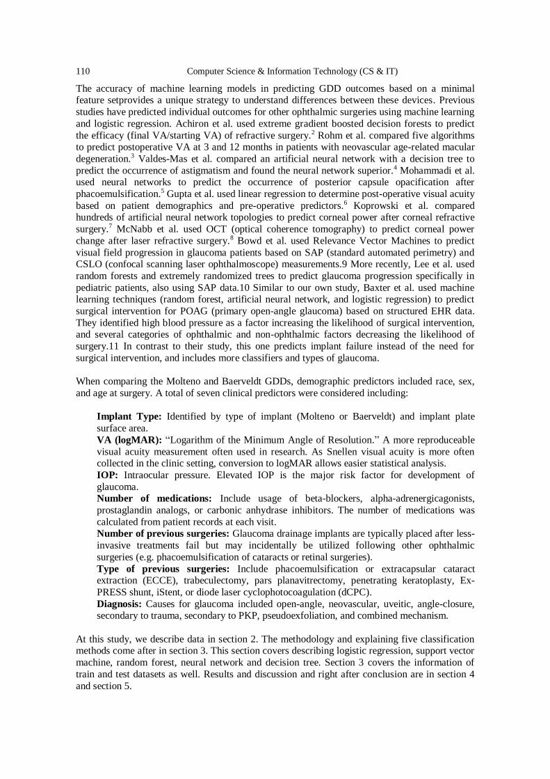
110 Computer Science & Information Technology (CS & IT)
The accuracy of machine learning models in predicting GDD outcomes based on a minimal feature setprovides a unique strategy to understand differences between these devices. Previous
studies have predicted individual outcomes for other ophthalmic surgeries using machine learning
and logistic regression. Achiron et al. used extreme gradient boosted decision forests to predict
the efficacy (final VA/starting VA) of refractive surgery.2 Rohm et al. compared five algorithms to predict postoperative VA at 3 and 12 months in patients with neovascular age-related macular
degeneration.3 Valdes-Mas et al. compared an artificial neural network with a decision tree to
predict the occurrence of astigmatism and found the neural network superior.4 Mohammadi et al. used neural networks to predict the occurrence of posterior capsule opacification after
phacoemulsification.5 Gupta et al. used linear regression to determine post-operative visual acuity
based on patient demographics and pre-operative predictors.6 Koprowski et al. compared hundreds of artificial neural network topologies to predict corneal power after corneal refractive
surgery.7 McNabb et al. used OCT (optical coherence tomography) to predict corneal power
change after laser refractive surgery.8 Bowd et al. used Relevance Vector Machines to predict
visual field progression in glaucoma patients based on SAP (standard automated perimetry) and CSLO (confocal scanning laser ophthalmoscope) measurements.9 More recently, Lee et al. used
random forests and extremely randomized trees to predict glaucoma progression specifically in
pediatric patients, also using SAP data.10 Similar to our own study, Baxter et al. used machine learning techniques (random forest, artificial neural network, and logistic regression) to predict
surgical intervention for POAG (primary open-angle glaucoma) based on structured EHR data.
They identified high blood pressure as a factor increasing the likelihood of surgical intervention, and several categories of ophthalmic and non-ophthalmic factors decreasing the likelihood of
surgery.11 In contrast to their study, this one predicts implant failure instead of the need for
surgical intervention, and includes more classifiers and types of glaucoma.
When comparing the Molteno and Baerveldt GDDs, demographic predictors included race, sex,
and age at surgery. A total of seven clinical predictors were considered including:
Implant Type: Identified by type of implant (Molteno or Baerveldt) and implant plate
surface area.
VA (logMAR): “Logarithm of the Minimum Angle of Resolution.” A more reproduceable
visual acuity measurement often used in research. As Snellen visual acuity is more often collected in the clinic setting, conversion to logMAR allows easier statistical analysis.
IOP: Intraocular pressure. Elevated IOP is the major risk factor for development of
glaucoma. Number of medications: Include usage of beta-blockers, alpha-adrenergicagonists,
prostaglandin analogs, or carbonic anhydrase inhibitors. The number of medications was
calculated from patient records at each visit. Number of previous surgeries: Glaucoma drainage implants are typically placed after less-
invasive treatments fail but may incidentally be utilized following other ophthalmic
surgeries (e.g. phacoemulsification of cataracts or retinal surgeries).
Type of previous surgeries: Include phacoemulsification or extracapsular cataract extraction (ECCE), trabeculectomy, pars planavitrectomy, penetrating keratoplasty, Ex-
PRESS shunt, iStent, or diode laser cyclophotocoagulation (dCPC).
Diagnosis: Causes for glaucoma included open-angle, neovascular, uveitic, angle-closure, secondary to trauma, secondary to PKP, pseudoexfoliation, and combined mechanism.
At this study, we describe data in section 2. The methodology and explaining five classification methods come after in section 3. This section covers describing logistic regression, support vector
machine, random forest, neural network and decision tree. Section 3 covers the information of
train and test datasets as well. Results and discussion and right after conclusion are in section 4
and section 5.

Computer Science & Information Technology (CS & IT) 111
111
2. DATA DESCRIPTION Of 62 patients analyzed, 26 (41%) were determined to have device failure. Follow-up time was
573±245.45 days, (range 133-1037 days). Patient samples were balanced between male and
female. White race was three times more common than Black race and there was only one Asian
patient (Tables 1 and 2). Implant failure was defined as final IOP was greater than or equal to 18, less than 20% reduction from pre-operative levels, or if repeat surgery for glaucoma was required
(this did not include in-clinic procedures that did not indicate failure of the device itself). By the
last recorded appointment, 35% (22) of patients had a failing IOP and 19% (12) required additional surgery. No patients in this group experienced loss of light perception.
Table 1: Number of participants by race and sex
Race Male Female Total
Asian 1 0 1
Black 8 8 16
White 24 21 45
Total 33 29 62
Table 2: Average Age at Surgery by Race and Sex
Race Male Female Average
Asian 72±0 (n = 1) - 72±0 (1 total)
Black 61.9±9.7 (n = 8) 68.9±6.53 (8 total) 65.4±8.1 (28 total)
White 65.8±12.2 (n = 24) 69.4±6.53 (21 total) 67.6±9.4 (58 total)
Average 65.0±11.22 ( 33total) 69.2±6.53 (29 total) 67.1±8.9 (62 total)
A total of 42 patients received a BaerveldtGDD (67%) and 20 received a Molteno implant (27%).
Forty-eight (77%) patients had surgery prior to placement of a GDD. Twelve patients (19%)
required repeat surgery after initial placement of a GDD. Open-angle glaucoma was the most common underlying diagnosis (61%, n = 38) with combined mechanism (11%, n = 5) and chronic
angle-closure (8%, n = 5) being less common. There were also individual patients with either
neovascular, uveitic, traumatic, or pseudo exfoliation glaucoma. A diagnosis of "Other" was
given for 8% of the patients, which indicated a singular diagnosis was not able to be determined from chart review.
3. METHODOLOGY All models in this study were validated using three-fold stratified cross validation, and all but the
neural net were developed using recursive feature elimination and grid searches. To prevent data
leakage, final validation, grid searching, and feature selection were performed in separate cross
validation loops, as recommended by Krstajic et al.12 In the outer loop, the final model was tested; in the middle loop, the best hyper parameters were chosen; and in the inner loop, the best
feature subsets were selected. Within each loop, three-fold stratified cross-validation was used.
Scaling and centering for continuous variables was performed as part of the model fitting procedure. The Logistic Regression, SVM, Decision Tree, and Random Forest classifiers were
implemented in Python using Scikit-Learn,13 and the Neural Network classifier was implemented
in R using the caret package.14

112 Computer Science & Information Technology (CS & IT)
3.1. Logistic Regression
Logistic regression, traditionally used for modeling, determines the class of each input variable
by multiplying each feature by a constant, adding a bias term, and applying the logistic function. Any outcome above 0.5 is rounded to 1; any outcome below 0.5 is rounded to 0. The optimal
logistic regression classifier used L2 regularization and a C parameter of 1, had an accuracy of
0.66±0.08 and a ROC (Receiver Operating Characteristic) of 0.67±0.08. Based on the coefficients of the logistic regression model listed in Table 3, Black race and initially taking beta-
blockers is associated with implant failure.
Feature Sign Coefficient
Black race + 0.83
Initially taking Beta Blockers + 0.63
White - 0.37
Initially taking Carbonic Anhydrase - 0.36
Baerveldt 350 mm2 - 0.28
Table 3: Feature Coefficients of Logistic Regression Classifier
3.2. Support Vector Machine (SVM)
A Support Vector Machine uses several data points (support vectors) to find the hyperplanes
separating data classes that allow identification of a hyperplane giving the maximum margin. The best classifier had a cost parameter of 0. Table 4 shows the feature coefficients of SVM
classifier.15
0.83
0.63
-0.37 -0.36-0.28
Black Initially taking
Beta Blockers
White Initially taking
Carbonic
Anhydrase
Baerveldt 350
mm2

Computer Science & Information Technology (CS & IT) 113
113
Feature Sign Coefficient
Combined tube placement and
phacoemulsification - 2
Black race + 1.41
No previous surgeries - 1
Baerveldt 350 mm2 - 0.7
Previous Phacoemulsification or ECCE - 0.6
Initially taking beta blockers + 0.59
Primary Open-Angle Glaucoma + 0.49
Previous Trabeculectomy - 0.36
Initially taking carbonic anhydrase inhibitor - 0.34
Initial VA (logMAR) + 0.28
Table 4: Feature Coefficients of SVM Classifier
Like regression, race and initially taking beta-blockers have the most weight in causing implant
failure. Primary Open-Angle Glaucoma show possibility of implant failure too. The SVM classifier had an accuracy of 0.61%±0.03 and a ROC AUC of 0.62±0.03.
3.3. Decision Tree
A decision tree repeatedly picks a threshold to divide data until it places all data items in groups
(mostly) of the same class. First, it finds the threshold for all features dividing data most cleanly. Then it chooses features producing the cleanest split and repeats the process separately for the
data on each side of the split. The algorithm stops when the data divide into pure groups or when
the number of points in each group is too small to divide further without overfitting15. We used a
minimum of three data points per leaf nodeand the Gini impurity measure.
-2
1.41
-1
-0.7-0.6
0.590.49
-0.36 -0.34
0.28
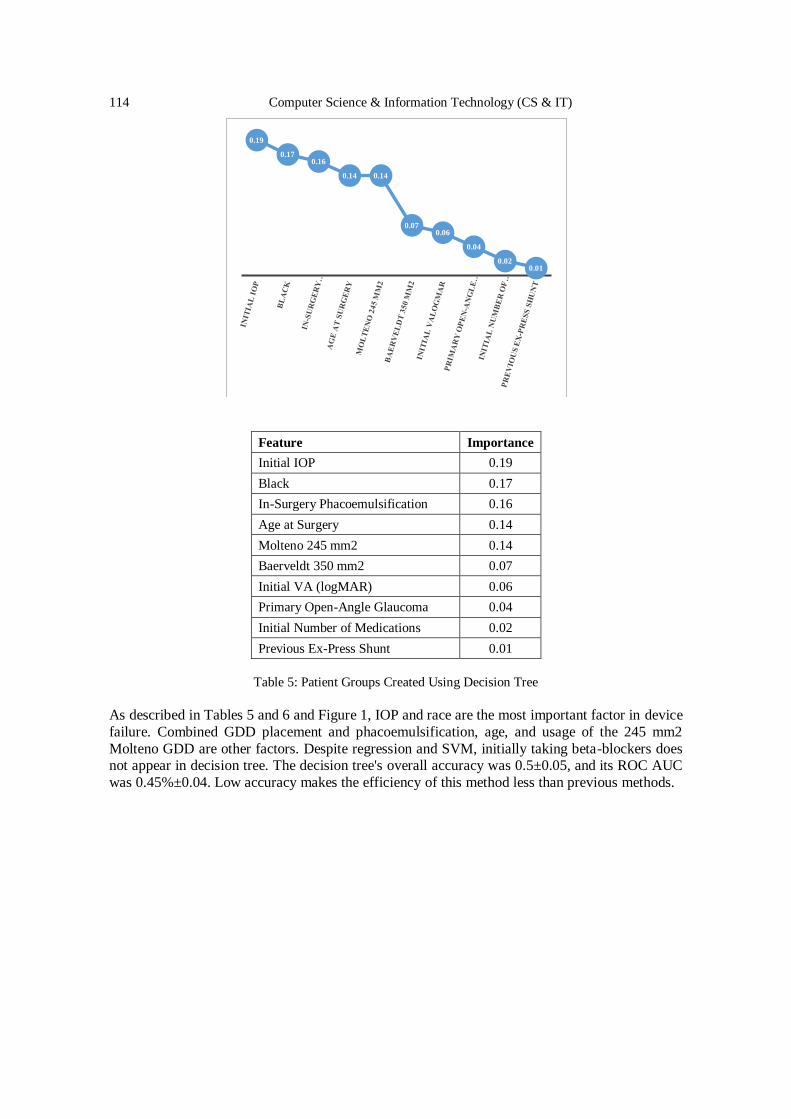
114 Computer Science & Information Technology (CS & IT)
Feature Importance
Initial IOP 0.19
Black 0.17
In-Surgery Phacoemulsification 0.16
Age at Surgery 0.14
Molteno 245 mm2 0.14
Baerveldt 350 mm2 0.07
Initial VA (logMAR) 0.06
Primary Open-Angle Glaucoma 0.04
Initial Number of Medications 0.02
Previous Ex-Press Shunt 0.01
Table 5: Patient Groups Created Using Decision Tree
As described in Tables 5 and 6 and Figure 1, IOP and race are the most important factor in device
failure. Combined GDD placement and phacoemulsification, age, and usage of the 245 mm2
Molteno GDD are other factors. Despite regression and SVM, initially taking beta-blockers does not appear in decision tree. The decision tree's overall accuracy was 0.5±0.05, and its ROC AUC
was 0.45%±0.04. Low accuracy makes the efficiency of this method less than previous methods.
0.19
0.170.16
0.14 0.14
0.070.06
0.04
0.020.01

Computer Science & Information Technology (CS & IT) 115
115
Figure 1: Decision Tree of Glaucoma Data
Table 6: Patient Groups Created Using Decision Tree
Group Characteristics Patient Features
Gro
up
Nu
mb
er
Decis
ion
Co
un
t
Nu
mb
er o
f
fais
ucc
esse
s
Nu
mb
er o
f fa
ilu
res
Gin
i
In-S
urg
ery
Ph
aco
em
uls
ific
ati
on
Bla
ck
Ag
e a
t S
urg
ery
Mo
lten
o 2
45
mm
2
Init
ial
IOP
Prim
ary
Op
en
-An
gle
Gla
uco
ma
Prev
iou
s E
x-P
ress
Sh
un
t
Init
ial
Nu
mb
er o
f
Med
ica
tio
ns
Init
ial
VA
log
MA
R
Ba
erv
eld
t 3
50
mm
2
0 Success 8 8 0 0 False Any <=
75.5 Any Any Any Any
An
y Any Any
1 Success 3 2 1 0.4 False Any >
75.5 Any Any Any Any
An
y Any Any
2 Failure 7 0 7 0 True False Any Any Any Any Any An
y Any False
3 Success 4 2 2 0.5 True False Any Any Any Any Any An
y Any True
4 Failure 4 0 4 0 True True Any False Any Any Any An
y
<=
0.44 Any
5 Success 4 2 2 0.5 True True Any False Any Any Any An
y
>
0.44 Any
6 Failure 3 0 3 0 True True <=
73.5 True <= 15.75 Any Any
An
y Any Any
7 Success 4 3 1 0.4 True True <=
73.5 True
21.0 <= x <
15.75
Fals
e Any
An
y Any Any
8 Failure 4 1 3 0.4 True True <=
73.5 True
38.0 <= x <
21.0
Fals
e Any
An
y Any Any
9 Success 3 2 1 0.4 True True <=
73.5 True > 38.0
Fals
e Any
An
y Any Any
10 Success 3 2 1 0.4 True True <=
73.5 True > 15.75 True False
An
y Any Any
11 Success 4 4 0 0 True True <=
73.5 True > 15.75 True True
<=
3.5 Any Any
12 Success 3 2 1 0.4 True True <=
73.5 True > 15.75 True True
>
3.5 Any Any
13 Success 8 8 0 0 True True >
73.5 True Any Any Any
An
y Any Any
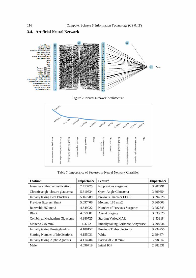
116 Computer Science & Information Technology (CS & IT)
3.4. Artificial Neural Network
Figure 2: Neural Network Architecture
Table 7: Importance of Features in Neural Network Classifier
Feature Importance Feature Importance
In-surgery Phacoemusification 7.413775 No previous surgeries 3.987791
Chronic angle-closure glaucoma 5.810634 Open-Angle Glaucoma 3.899654
Initially taking Beta Blockers 5.167789 Previous Phaco or ECCE 3.894626
Previous Express Shunt 5.097406 Molteno 185 mm2 3.866003
Baerveldt 350 mm2 4.649922 Number of Previous Surgeries 3.782343
Black 4.559001 Age at Surgery 3.535026
Combined Mechanism Glaucoma 4.380725 Starting VAlogMAR 3.53318
Molteno 245 mm2 4.3772 Initially taking Carbonic Anhydrase 3.298634
Initially taking Prostaglandins 4.180157 Previous Trabeculectomy 3.234256
Starting Number of Medications 4.155031 White 2.994674
Initially taking Alpha Agonists 4.114784 Baerveldt 250 mm2 2.98814
Male 4.096719 Initial IOP 2.982531
In-su
rgery
Ph
aco
em
usifica
tion
Ch
ron
ic a
ng
le-closu
re gla
ucom
a
Initia
lly ta
kin
g B
eta B
lock
ers
Prev
iou
s Exp
ress S
hu
nt
Baerv
eldt 3
50
mm
2
Bla
ck
Co
mb
ined
Mech
an
ism
Gla
uco
ma
Molten
o 2
45
mm
2
Initia
lly ta
kin
g P
rosta
gla
nd
ins
Sta
rting
Nu
mb
er o
f Med
icatio
ns
Initia
lly ta
kin
g A
lph
a A
go
nists
Male

Computer Science & Information Technology (CS & IT) 117
117
A feed-forward artificial neural network imitates biological neural tissue using sequential layers of "neurons" that transform the underlying data and pass it on to the next layer. The root of a
neural net is a perceptron: two or more inputs connected to a neuron, which then multiplies each
input by a weight, adds an intercept, and applies an output function to the result. In a single-layer
neural network, many perceptrons extract information from the underlying features, and a final neuron (or more for multiclass classification) combines the output from these nodes15. A single-
layer network with 25 hidden nodes (Fig. 2) was trained on the data. Combined GDD placement
and phacoemulsification was indicated as the most important factor in failure. Chronic angle-closure glaucoma and initially taking beta-blockers were also associated with therapy failure,
though to a lesser extent. Race with importance = 4.6 shows high effect on failure. The accuracy
was 0.53±0.11 and the ROC AUC was 0.52±0.10.
3.5. Random Forest
Table 8: Importance of Features in Random Forest Classifier
Feature Importance
Age at Surgery 0.25
Initial IOP 0.2
Initial VAlogMAR 0.12
Black 0.07
Molteno 245 mm2 0.07
Initial Number of Medications 0.06
On beta-blocker prior to surgery 0.06
Combined device and
phacoemulsification
0.06
Number of Previous Surgeries 0.05
Primary Open-Angle Glaucoma 0.03
On CAI prior to surgery 0.02
Previous Ex-Press Shunt 0.01
A random forest averages the predictions of multiple decision trees trained on subsets of the
data15. Using ten decision trees, the algorithm identified age at surgery, initial IOP, and visual acuity as the most important factors determining device failure. Race and utilization of the larger
Molteno device (245 mm2) were associated with device failure, though to a lesser degree. The
overall ROC AUC was 0.58±0.1, and the overall accuracy was 0.58±0.13.
0.25
0.2
0.12
0.07 0.070.06 0.06 0.06
0.050.03
0.020.01
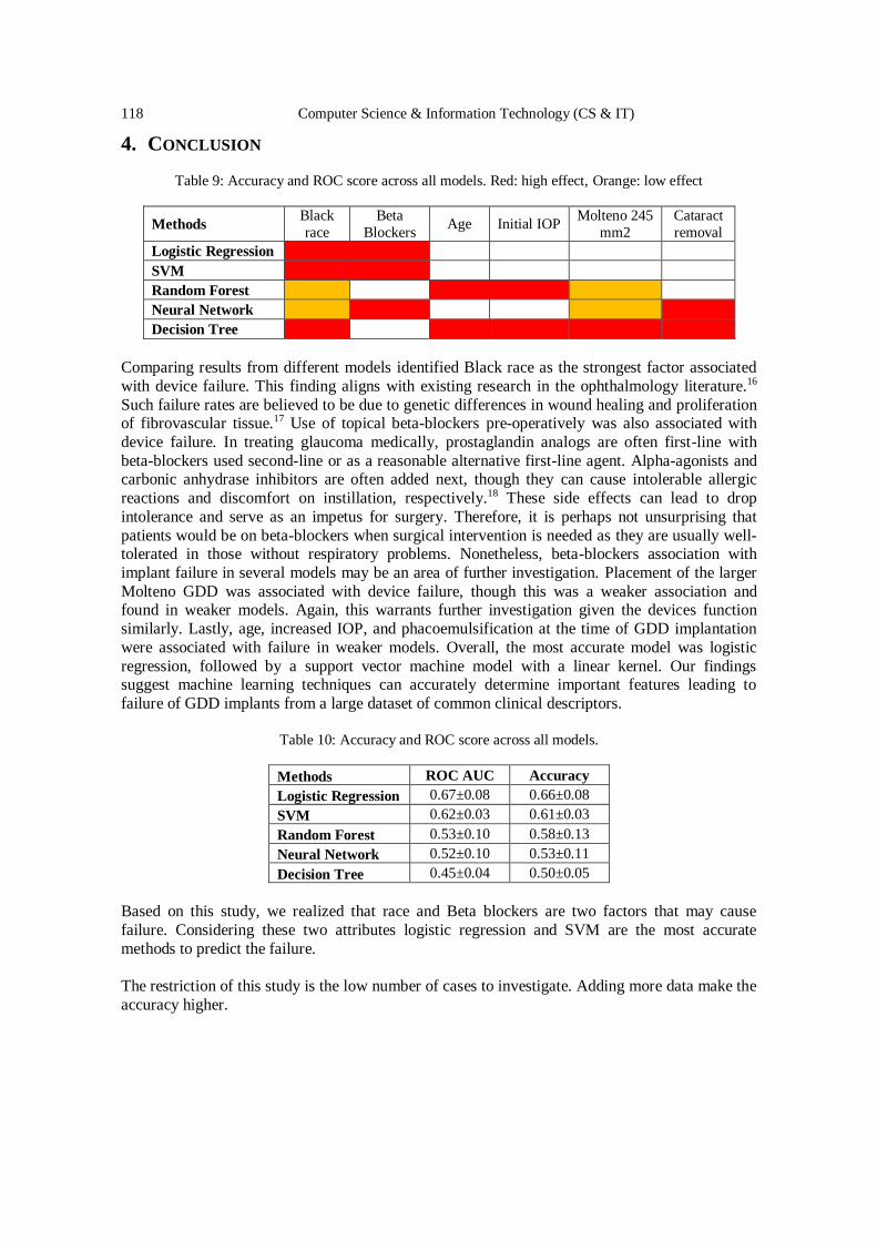
118 Computer Science & Information Technology (CS & IT)
4. CONCLUSION
Table 9: Accuracy and ROC score across all models. Red: high effect, Orange: low effect
Methods Black
race
Beta
Blockers Age Initial IOP
Molteno 245
mm2
Cataract
removal
Logistic Regression
SVM
Random Forest
Neural Network
Decision Tree
Comparing results from different models identified Black race as the strongest factor associated
with device failure. This finding aligns with existing research in the ophthalmology literature.16
Such failure rates are believed to be due to genetic differences in wound healing and proliferation of fibrovascular tissue.17 Use of topical beta-blockers pre-operatively was also associated with
device failure. In treating glaucoma medically, prostaglandin analogs are often first-line with
beta-blockers used second-line or as a reasonable alternative first-line agent. Alpha-agonists and carbonic anhydrase inhibitors are often added next, though they can cause intolerable allergic
reactions and discomfort on instillation, respectively.18 These side effects can lead to drop
intolerance and serve as an impetus for surgery. Therefore, it is perhaps not unsurprising that
patients would be on beta-blockers when surgical intervention is needed as they are usually well-tolerated in those without respiratory problems. Nonetheless, beta-blockers association with
implant failure in several models may be an area of further investigation. Placement of the larger
Molteno GDD was associated with device failure, though this was a weaker association and found in weaker models. Again, this warrants further investigation given the devices function
similarly. Lastly, age, increased IOP, and phacoemulsification at the time of GDD implantation
were associated with failure in weaker models. Overall, the most accurate model was logistic
regression, followed by a support vector machine model with a linear kernel. Our findings suggest machine learning techniques can accurately determine important features leading to
failure of GDD implants from a large dataset of common clinical descriptors.
Table 10: Accuracy and ROC score across all models.
Methods ROC AUC Accuracy
Logistic Regression 0.67±0.08 0.66±0.08
SVM 0.62±0.03 0.61±0.03
Random Forest 0.53±0.10 0.58±0.13
Neural Network 0.52±0.10 0.53±0.11
Decision Tree 0.45±0.04 0.50±0.05
Based on this study, we realized that race and Beta blockers are two factors that may cause
failure. Considering these two attributes logistic regression and SVM are the most accurate
methods to predict the failure.
The restriction of this study is the low number of cases to investigate. Adding more data make the
accuracy higher.
Computer Science & Information Technology (CS & IT) 119
119
AUTHOR CONTRIBUTIONS
PM: Preprocessed data, wrote the code in R and Python, investigated and analyzed the data, and
wrote the paper. MD: Prepared the data and wrote the data description. AS: Provided the data and advised the biological and learning approaches. BR: Supervised the computational approaches
and conceived the idea of the paper. All authors commented on this paper.
REFERENCES
[1] D. L. Budenz et al., “Five-Year Treatment Outcomes in the Ahmed Baerveldt Comparison Study,”
Ophthalmology, vol. 122, no. 2, pp. 308–316, Feb. 2015, doi: 10.1016/j.ophtha.2014.08.043.
[2] A. Achiron et al., “Predicting Refractive Surgery Outcome: Machine Learning Approach With Big
Data,” J Refract Surg, vol. 33, no. 9, pp. 592–597, Sep. 2017, doi: 10.3928/1081597X-20170616-03.
[3] M. Rohm et al., “Predicting Visual Acuity by Using Machine Learning in Patients Treated for
Neovascular Age-Related Macular Degeneration,” Ophthalmology, vol. 125, no. 7, pp. 1028–1036,
Jul. 2018, doi: 10.1016/j.ophtha.2017.12.034. [4] M. A. Valdes-Mas, J. D. Martin, M. J. Ruperez, C. Peris, and C. Monserrat, “Machine learning for
predicting astigmatism in patients with keratoconus after intracorneal ring implantation,” in IEEE-
EMBS International Conference on Biomedical and Health Informatics (BHI), Valencia, Spain, Jun.
2014, pp. 756–759, doi: 10.1109/BHI.2014.6864474.
[5] S.-F. Mohammadi et al., “Using artificial intelligence to predict the risk for posterior capsule
opacification after phacoemulsification:,” Journal of Cataract & Refractive Surgery, vol. 38, no. 3, pp.
403–408, Mar. 2012, doi: 10.1016/j.jcrs.2011.09.036.
[6] M. Gupta, P. Gupta, P. K. Vaddavalli, and A. Fatima, “Predicting Post-operative Visual Acuity for
LASIK Surgeries,” in Advances in Knowledge Discovery and Data Mining, vol. 9651, J. Bailey, L.
Khan, T. Washio, G. Dobbie, J. Z. Huang, and R. Wang, Eds. Cham: Springer International
Publishing, 2016, pp. 489–501. [7] R. Koprowski, M. Lanza, and C. Irregolare, “Corneal power evaluation after myopic corneal
refractive surgery using artificial neural networks,” BioMed EngOnLine, vol. 15, no. 1, p. 121, Dec.
2016, doi: 10.1186/s12938-016-0243-5.
[8] R. P. McNabb, S. Farsiu, S. S. Stinnett, J. A. Izatt, and A. N. Kuo, “Optical Coherence Tomography
Accurately Measures Corneal Power Change from Laser Refractive Surgery,” Ophthalmology, vol.
122, no. 4, pp. 677–686, Apr. 2015, doi: 10.1016/j.ophtha.2014.10.003.
[9] C. Bowd et al., “Predicting Glaucomatous Progression in Glaucoma Suspect Eyes Using Relevance
Vector Machine Classifiers for Combined Structural and Functional Measurements,” Invest.
Ophthalmol. Vis. Sci., vol. 53, no. 4, p. 2382, Apr. 2012, doi: 10.1167/iovs.11-7951.
[10] J. Lee, Y. K. Kim, J. W. Jeoung, A. Ha, Y. W. Kim, and K. H. Park, “Machine learning classifiers-
based prediction of normal-tension glaucoma progression in young myopic patients,” Jpn J
Ophthalmol, vol. 64, no. 1, pp. 68–76, Jan. 2020, doi: 10.1007/s10384-019-00706-2. [11] S. L. Baxter, C. Marks, T.-T. Kuo, L. Ohno-Machado, and R. N. Weinreb, “Machine Learning-Based
Predictive Modeling of Surgical Intervention in Glaucoma Using Systemic Data From Electronic
Health Records,” American Journal of Ophthalmology, vol. 208, pp. 30–40, Dec. 2019, doi:
10.1016/j.ajo.2019.07.005.
[12] D. Krstajic, L. J. Buturovic, D. E. Leahy, and S. Thomas, “Cross-validation pitfalls when selecting
and assessing regression and classification models,” J Cheminform, vol. 6, no. 1, p. 10, Dec. 2014,
doi: 10.1186/1758-2946-6-10.
[13] F. Pedregosa et al., “Scikit-learn: Machine Learning in Python,” arXiv:1201.0490 [cs], Jun. 2018,
Accessed: Nov. 22, 2020. [Online]. Available: http://arxiv.org/abs/1201.0490.
[14] M. Kuhn, “Building Predictive Models in R Using the caret Package,” J. Stat. Soft., vol. 28, no. 5,
2008, doi: 10.18637/jss.v028.i05. [15] P.-N. Tan, M. Steinbach, and V. Kumar, Introduction to data mining, 1st ed. Boston: Pearson
Addison Wesley, 2006.
[16] “The advanced glaucoma intervention study (AGIS)*113. Comparison of treatment outcomes within
race: 10-year results,” Ophthalmology, vol. 111, no. 4, pp. 651–664, Apr. 2004, doi:
10.1016/j.ophtha.2003.09.025.

120 Computer Science & Information Technology (CS & IT)
[17] D. Broadway, I. Grierson, and R. Hitchings, “Racial differences in the results of glaucoma filtration
surgery: are racial differences in the conjunctival cell profile important?,” British Journal of
Ophthalmology, vol. 78, no. 6, pp. 466–475, Jun. 1994, doi: 10.1136/bjo.78.6.466.
[18] K. Inoue, “Managing adverse effects of glaucoma medications,” OPTH, p. 903, May 2014, doi:
10.2147/OPTH.S44708.
© 2020 By AIRCC Publishing Corporation. This article is published under the Creative Commons
Attribution (CC BY) license.

AUTHOR INDEX
Abdulelah Abdulkhaleq Mohammed Hassan 17
Alan I. Reed 99
Arsham Sheybani 109
Bahareh Rahmani 109
Byoung Jik Lee 93
Changyan Xiao 27
Dieuthuy Pham 27
Doruk Pancaroglu 41
Eric S. Pahl 99
Habeb Abdulkhaleq Mohammed Hassan 17
Hans J. Johnson 99
Hong Xiong 77
Isma Dahmani 65
Maxwell Dixon 109
Mhand Hifi 65
Minhtuan Ha 27
Paul Morrison 109
Qing Li 55
Ruiwen Zhang 55
Samah Boukhari 65
Tingwei Li 55
W. Nick Street 99
Yakoop Razzaz Hamoud Qasim 17
Yoshiaki OKUBO 01