Embed Size (px)
Citation preview

COMPUTER VISION

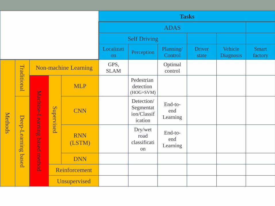
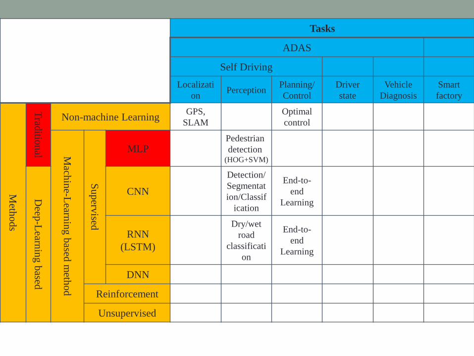
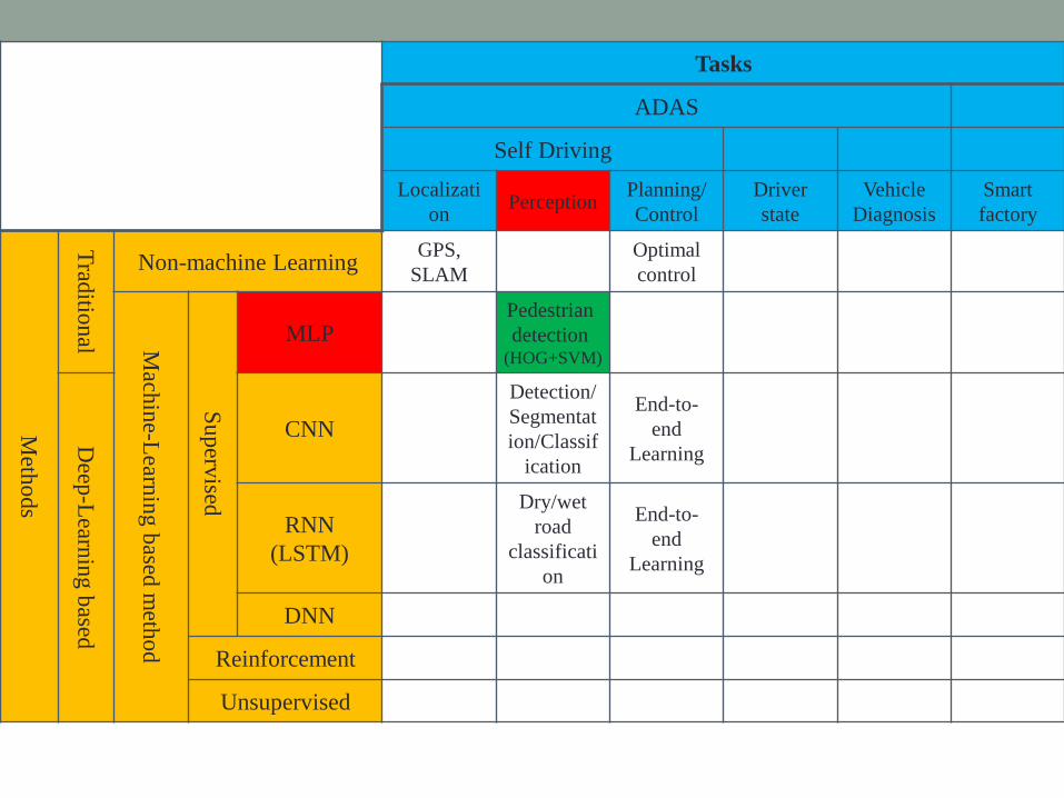
Tasks
ADAS
Self Driving
Localizati
onPerception
Planning/
Control
Driver
state
Vehicle
Diagnosis
Smart
factory
Meth
od
s
Trad
ition
al
Non-machine LearningGPS,
SLAM
Optimal
control
Mach
ine-L
earnin
gb
ased m
etho
d
Su
perv
ised
SVM
MLP
Pedestrian
detection(HOG+SVM)
Deep
-Learn
ing
based
CNN
Detection/
Segmentat
ion/Classif
ication
End-to-
end
Learning
RNN
(LSTM)
Dry/wet
road
classificati
on
End-to-
end
Learning
Behavior
Prediction/
Driver
identificati
on
*
DNN * *
Reinforcement *
Unsupervised *

Vision tasks
Object
recognition
Object
detection
Semantic
segmentation
Object
tracking
Visual
SLAM

Semantic segmentation
• Building/road/sky/object/grass/water/tree
Clement Farabet, Camille Couprie, Laurent Najman and Yann LeCun: Learning Hierarchical Features for Scene Labeling, IEEE Transactions
on Pattern Analysis and Machine Intelligence, August, 2013

Object tracking
Yi Wu, Jongwoo Lim, and Ming-Hsuan Yang, "Object Tracking Benchmark",
IEEE Transactions on Pattern Analysis and Machine Intelligence, 2015
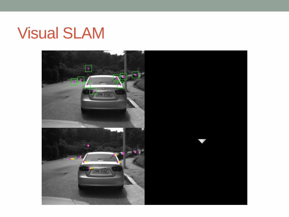
Visual SLAM

Tasks
ADAS
Self Driving
Localizati
onPerception
Planning/
Control
Driver
state
Vehicle
Diagnosis
Smart
factory
Meth
od
s
Trad
ition
al
Non-machine LearningGPS,
SLAM
Optimal
control
Mach
ine-L
earnin
gb
ased m
etho
d
Su
perv
ised
SVM
MLP
Pedestrian
detection(HOG+SVM)
Deep
-Learn
ing
based
CNN
Detection/
Segmentat
ion/Classif
ication
End-to-
end
Learning
RNN
(LSTM)
Dry/wet
road
classificati
on
End-to-
end
Learning
Behavior
Prediction/
Driver
identificati
on
*
DNN * *
Reinforcement *
Unsupervised *
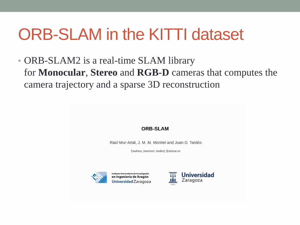
ORB-SLAM in the KITTI dataset
• ORB-SLAM2 is a real-time SLAM library
for Monocular, Stereo and RGB-D cameras that computes the
camera trajectory and a sparse 3D reconstruction
WHY UNDERSTANDING IMAGES IS
HARD?

Why understanding images is hard
Image
Very man
y sources
of variabil
ity
From J. Winn, MSR
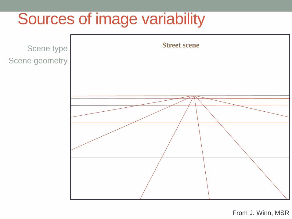
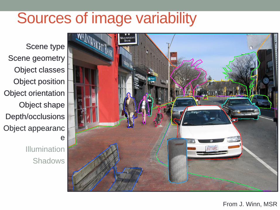
Sources of image variability
Scene type
Scene geometry
Street scene
From J. Winn, MSR

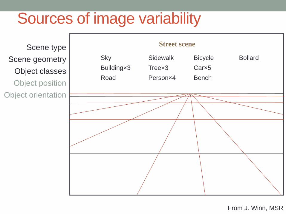
Sources of image variability
Scene type
Scene geometry
Object classes
Street scene
Sky
Building×3
Road
Sidewalk
Tree×3
Person×4
Bicycle
Car×5
Bench
Bollard
From J. Winn, MSR
Sources of image variability
Street scene
Sky
Building×3
Road
Sidewalk
Tree×3
Person×4
Bicycle
Car×5
Bench
Bollard
Scene type
Scene geometry
Object classes
Object position
Object orientation
From J. Winn, MSR
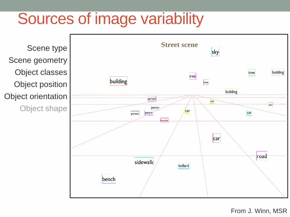
Sources of image variability
Scene type
Scene geometry
Object classes
Object position
Object orientation
Scene type
Scene geometry
Object classes
Object position
Object orientation
Object shape
Street scene
From J. Winn, MSR

Scene type
Scene geometry
Object classes
Object position
Object orientation
Object shape
Sources of image variability
Scene type
Scene geometry
Object classes
Object position
Object orientation
Object shape
Depth/occlusions
From J. Winn, MSR

Sources of image variability
Scene type
Scene geometry
Object classes
Object position
Object orientation
Object shape
Depth/occlusions
Scene type
Scene geometry
Object classes
Object position
Object orientation
Object shape
Depth/occlusions
Object appearan
ce
From J. Winn, MSR
Sources of image variability
Scene type
Scene geometry
Object classes
Object position
Object orientation
Object shape
Depth/occlusions
Object appearanc
e
Scene type
Scene geometry
Object classes
Object position
Object orientation
Object shape
Depth/occlusions
Object appearanc
e
Illumination
Shadows
From J. Winn, MSR

Sources of image variability
Scene type
Scene geometry
Object classes
Object position
Object orientation
Object shape
Depth/occlusions
Object appearanc
e
Illumination
Shadows
From J. Winn, MSR

Sources of image variability
Scene type
Scene geometry
Object classes
Object position
Object orientation
Object shape
Depth/occlusions
Object appearanc
e
Illumination
Shadows
Motion blur
Camera effects
From J. Winn, MSR

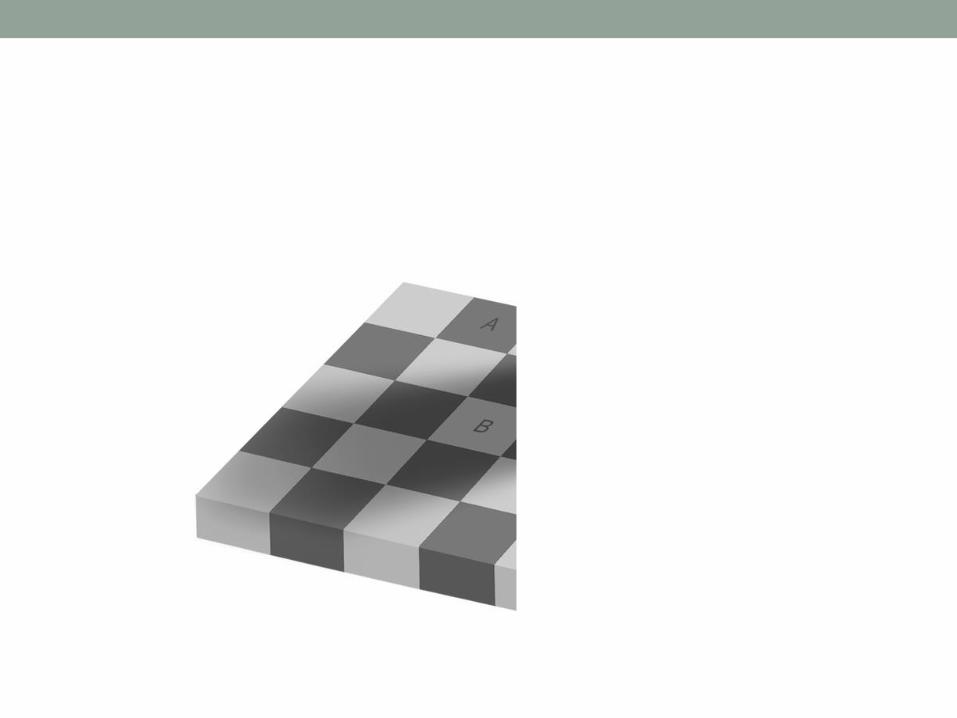
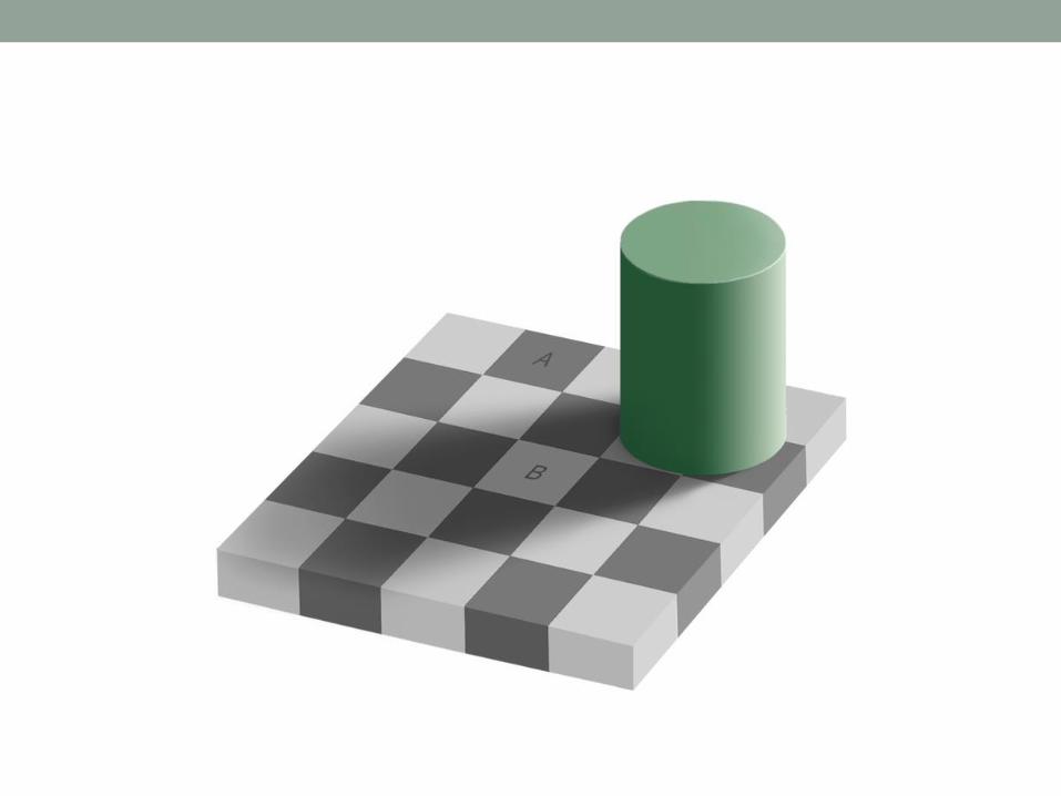
Computer vision problems
Scene type
Scene geometry
Object classes
Object position
Object orientation
Object shape
Depth/occlusions
Object appearanc
e
Illumination
Shadows
Motion blur
Camera effects
Now you see me


MACHINE LEARNINGNeural network을중심으로

Tasks
ADAS
Self Driving
Localizati
onPerception
Planning/
Control
Driver
state
Vehicle
Diagnosis
Smart
factory
Meth
od
s
Trad
ition
al
Non-machine LearningGPS,
SLAM
Optimal
control
Mach
ine-L
earnin
gb
ased m
etho
d
Su
perv
ised
MLPPedestrian
detection(HOG+SVM)
Deep
-Learn
ing
based
CNN
Detection/
Segmentat
ion/Classif
ication
End-to-
end
Learning
RNN
(LSTM)
Dry/wet
road
classificati
on
End-to-
end
Learning
DNN
Reinforcement
Unsupervised

LINEAR PERCEPTRON

뉴런: 신경망의기본단위
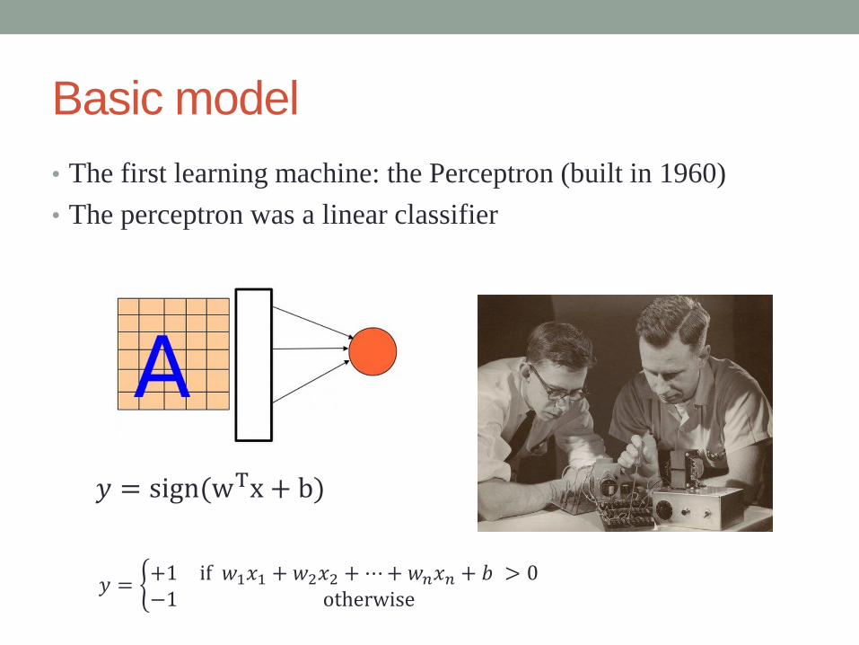
Basic model
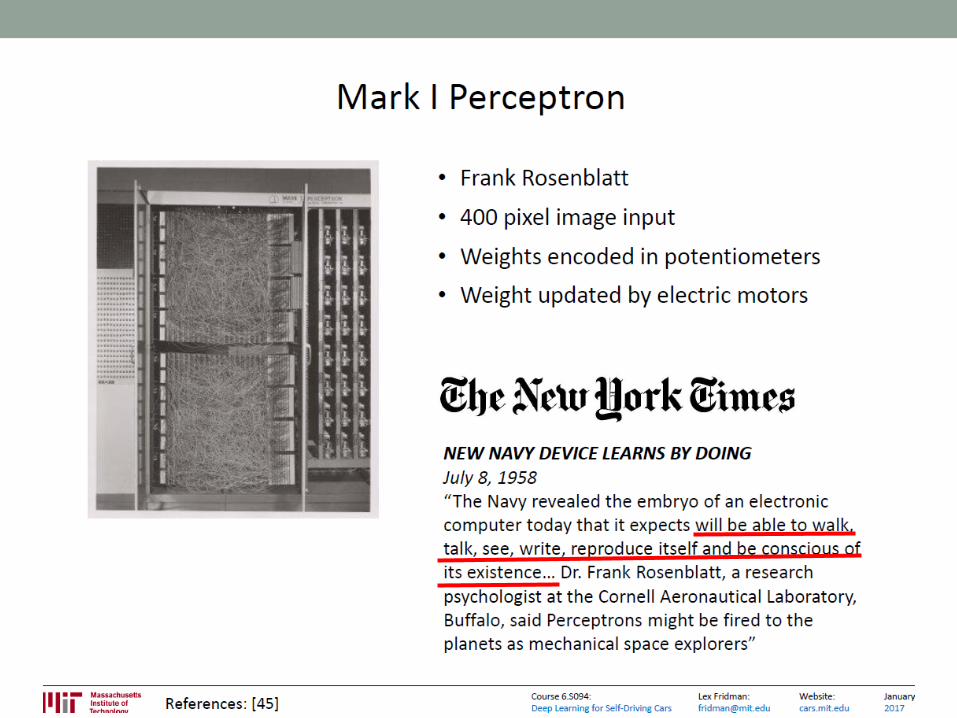
• The first learning machine: the Perceptron (built in 1960)
• The perceptron was a linear classifier
𝑦 = sign(wTx + b)
𝑦 = +1 if 𝑤1𝑥1 + 𝑤2𝑥2 +⋯+𝑤𝑛𝑥𝑛 + 𝑏 > 0−1 otherwise

Linear Perceptron
• The goal: Find the best line (or hyper-plane) to separate the training data.
• In two dimensions, the equation of the line is given by a line:
• 𝑎𝑥 + 𝑏𝑦 + 𝑐 = 0
• A better notation for n dimensions: treat each data point and the coefficients as vectors. Then the equation is given by:
• w⊤x + b = 0
Class (+1)Class (-1)
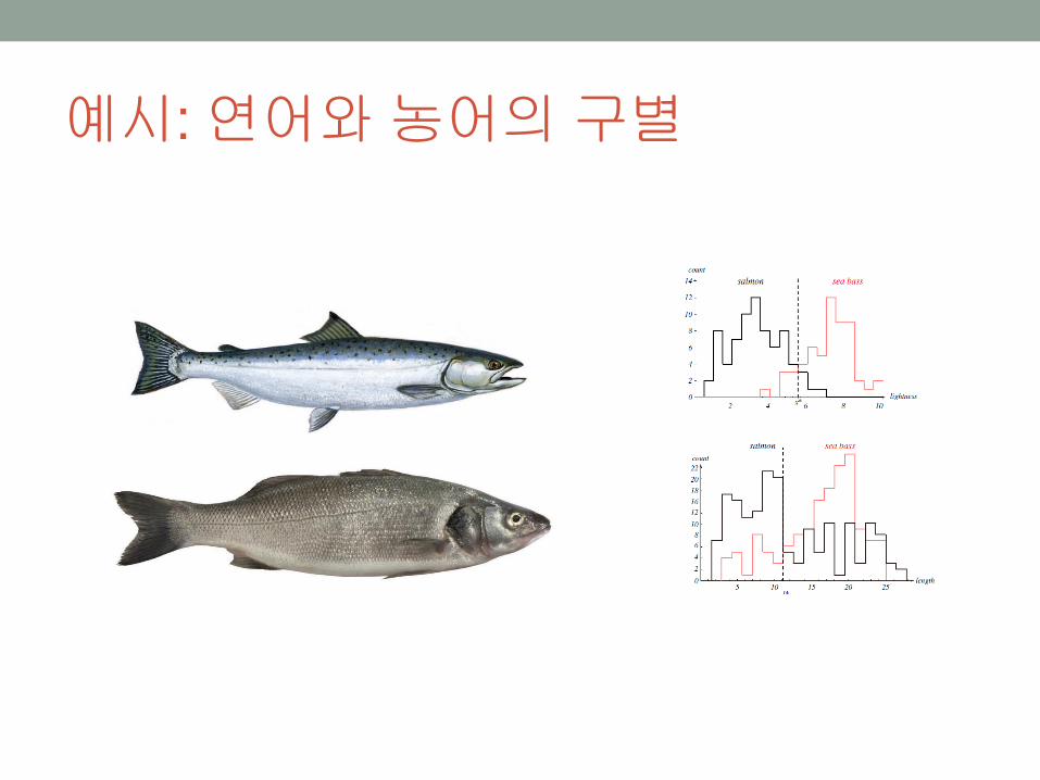
예시: 연어와농어의구별
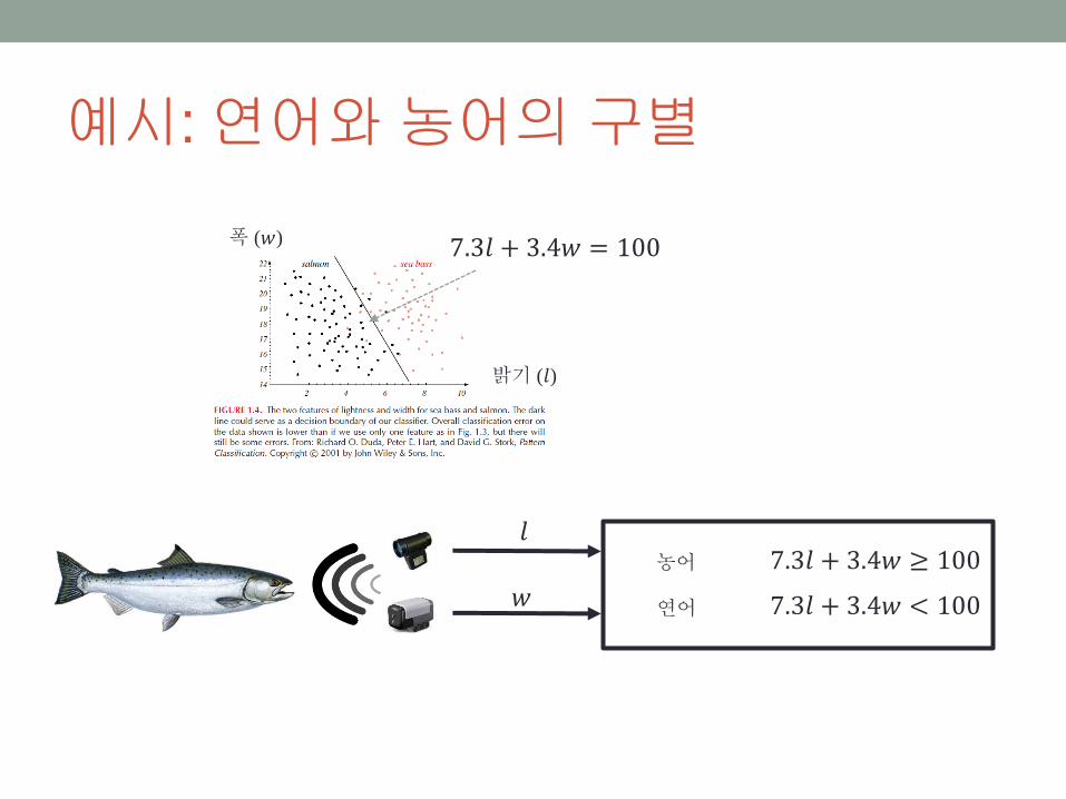
예시: 연어와농어의구별
밝기 (𝑙)
폭 (𝑤) 7.3𝑙 + 3.4𝑤 = 100
𝑙
𝑤
7.3𝑙 + 3.4𝑤 ≥ 100
7.3𝑙 + 3.4𝑤 < 100
농어
연어
4 2 2 4
0.2
0.4
0.6
0.8
1.0
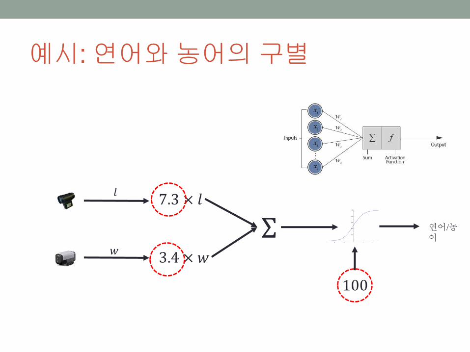
예시: 연어와농어의구별
𝑙
𝑤
7.3 × 𝑙
3.4 × 𝑤
Σ
100
연어/농어

Artificial Neuron
𝑤𝑇𝑥 𝑔(𝑤𝑇𝑥)
Activation function (non-linear)

Artificial Neuron
• However, it cannot solve non-linearly-separable problems
MULTI-LAYER PERCEPTRON

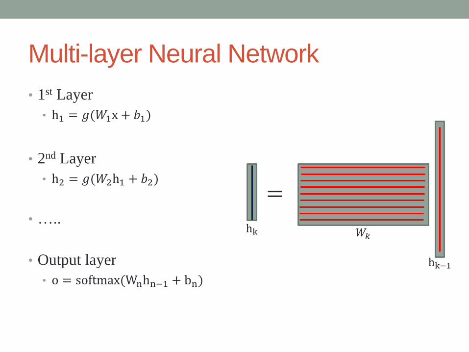
Multi-layer Neural Network
• 1st Layer
• h1 = 𝑔(𝑊1x + 𝑏1)
• 2nd Layer
• h2 = 𝑔(𝑊2h1 + 𝑏2)
• …..
• Output layer
• o = softmax(Wnhn−1 + bn)
=
hk
hk−1
𝑊𝑘

4 2 2 4
1.0
0.5
0.5
1.0
4 2 2 4
0.2
0.4
0.6
0.8
1.0
Activation function 𝑔(⋅)
• Sigmoid activation function
• Squashes the neuron’s pre-activation between 0 and 1
• Always positive/Bounded/Strictly increasing
• Hyperbolic tangent (‘‘tanh’’) activation function
• Squashes the neuron’s pre-activation between -1 and 1
• Bounded/Strictly increasing
𝑔 𝑥 =1
1 + exp(−𝑥)
𝑔 𝑥 = tanh 𝑥 =exp 𝑥 − exp(−𝑥)
exp(𝑥) + exp(−𝑥)

Activation function 𝑔(⋅)
• Rectified linear activation function (ReLU)
• Bounded below by 0
• Not upper bounded
• Strictly increasing
𝑔 𝑎 = rectlin 𝑎 = max 0, 𝑎
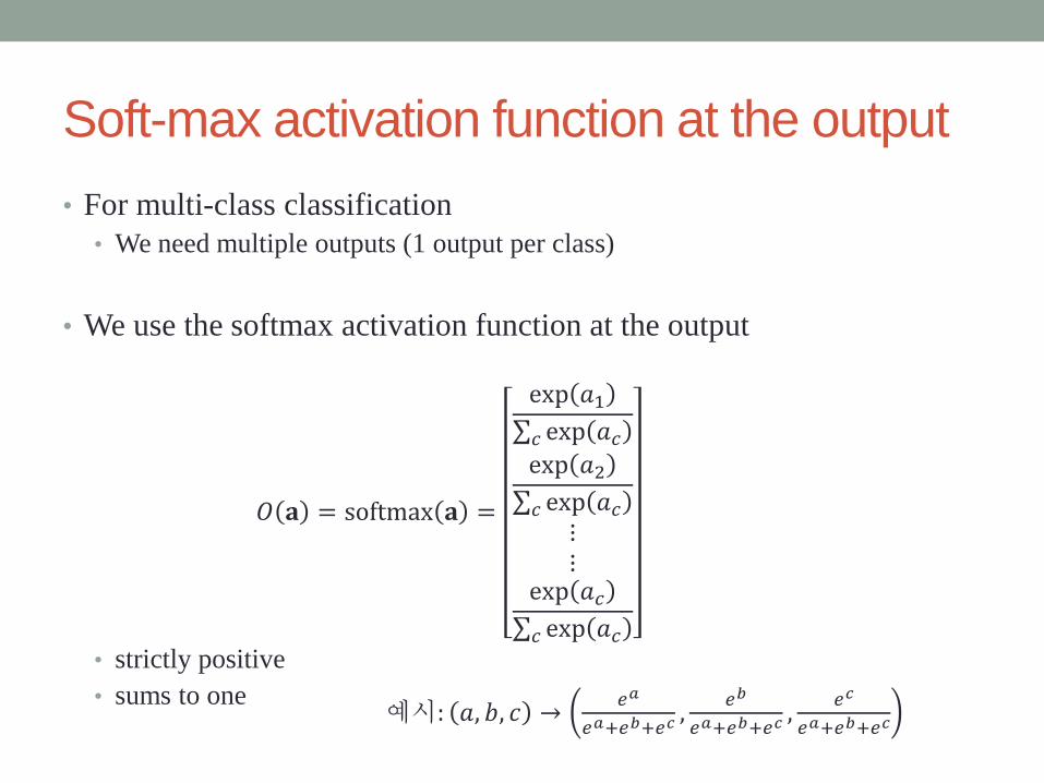
Soft-max activation function at the output
• For multi-class classification
• We need multiple outputs (1 output per class)
• We use the softmax activation function at the output
• strictly positive
• sums to one
𝑂 𝐚 = softmax 𝐚 =
exp 𝑎1 𝑐 exp 𝑎𝑐exp 𝑎2
𝑐 exp 𝑎𝑐⋮⋮
exp 𝑎𝑐 𝑐 exp 𝑎𝑐
예시: 𝑎, 𝑏, 𝑐 →𝑒𝑎
𝑒𝑎+𝑒𝑏+𝑒𝑐,
𝑒𝑏
𝑒𝑎+𝑒𝑏+𝑒𝑐,
𝑒𝑐
𝑒𝑎+𝑒𝑏+𝑒𝑐

Example (character recognition example)
𝑥 ∈ 0,1 10×14
𝑝(𝑐 = "0"|𝑥)
𝑝(𝑐 = "1"|𝑥)
𝑝(𝑐 = "9"|𝑥)
⋮
140 inputs
Layer 1
with 12 perceptrons
Layer 2
with 10 perceptrons
Each having 12 inputs𝑊1 ∈ ℜ140×12
𝑊2 ∈ ℜ12×10
softm
ax
𝑏1 ∈ ℜ12
𝑏2 ∈ ℜ10

TRAINING OF MULTI-LAYER
PERCEPTRON
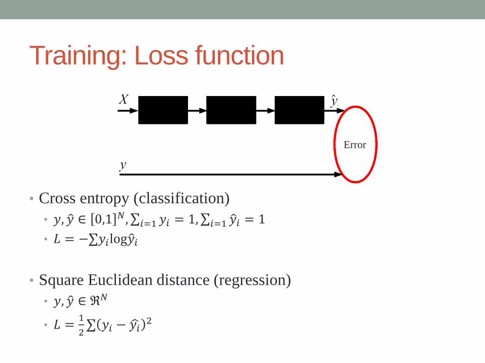
Training: Loss function
• Cross entropy (classification)
• 𝑦, 𝑦 ∈ 0,1 𝑁, 𝑖=1𝑦𝑖 = 1, 𝑖=1 𝑦𝑖 = 1
• 𝐿 = − 𝑦𝑖log 𝑦𝑖
• Square Euclidean distance (regression)
• 𝑦, 𝑦 ∈ ℜ𝑁
• 𝐿 =1
2 𝑦𝑖 − 𝑦𝑖
2
Error
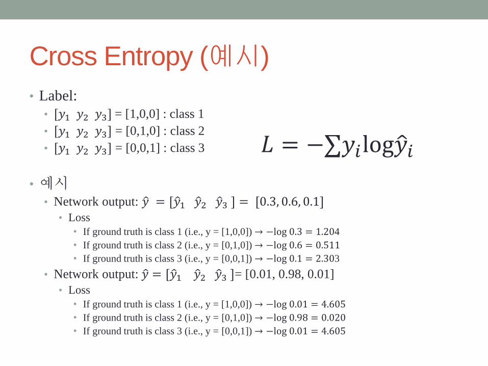
Cross Entropy (예시)
• Label:
• [𝑦1 𝑦2 𝑦3] = [1,0,0] : class 1
• [𝑦1 𝑦2 𝑦3] = [0,1,0] : class 2
• [𝑦1 𝑦2 𝑦3] = [0,0,1] : class 3
• 예시• Network output: 𝑦 = [ 𝑦1 𝑦2 𝑦3 ] = [0.3, 0.6, 0.1]
• Loss
• If ground truth is class 1 (i.e., y = [1,0,0]) → −log 0.3 = 1.204
• If ground truth is class 2 (i.e., y = [0,1,0]) → −log 0.6 = 0.511
• If ground truth is class 3 (i.e., y = [0,0,1]) → −log 0.1 = 2.303
• Network output: 𝑦 = [ 𝑦1 𝑦2 𝑦3 ]= [0.01, 0.98, 0.01]
• Loss
• If ground truth is class 1 (i.e., y = [1,0,0]) → −log 0.01 = 4.605
• If ground truth is class 2 (i.e., y = [0,1,0]) → −log 0.98 = 0.020
• If ground truth is class 3 (i.e., y = [0,0,1]) → −log 0.01 = 4.605
𝐿 = − 𝑦𝑖log 𝑦𝑖
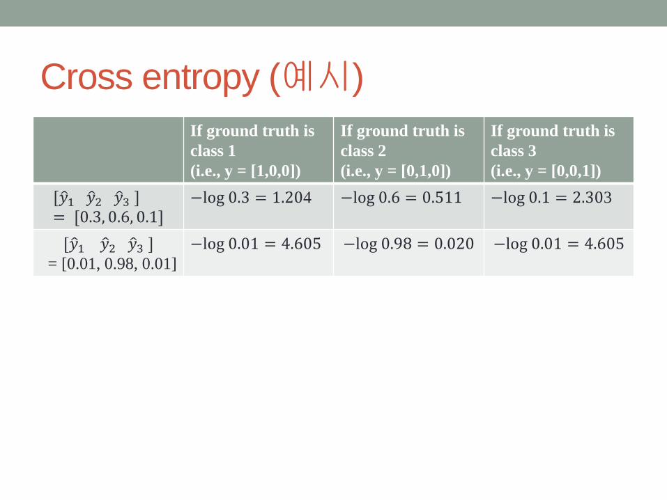
Cross entropy (예시)
If ground truth is
class 1
(i.e., y = [1,0,0])
If ground truth is
class 2
(i.e., y = [0,1,0])
If ground truth is
class 3
(i.e., y = [0,0,1])
[ 𝑦1 𝑦2 𝑦3 ]= [0.3, 0.6, 0.1]
−log 0.3 = 1.204 −log 0.6 = 0.511 −log 0.1 = 2.303
[ 𝑦1 𝑦2 𝑦3 ]= [0.01, 0.98, 0.01]
−log 0.01 = 4.605 −log 0.98 = 0.020 −log 0.01 = 4.605

Forward/Backward propagation
• Chain rule
𝑊𝑛𝑒𝑤 = 𝑊𝑜𝑙𝑑 − 𝜂𝑑𝐿
𝑑𝑊
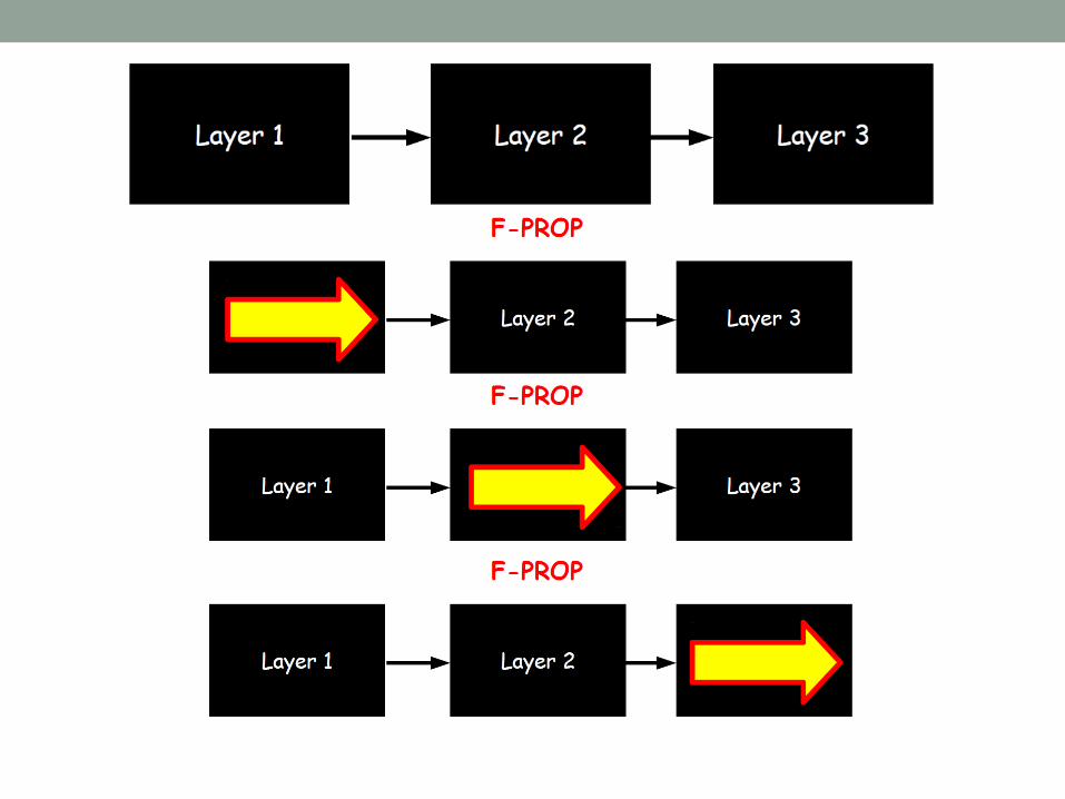
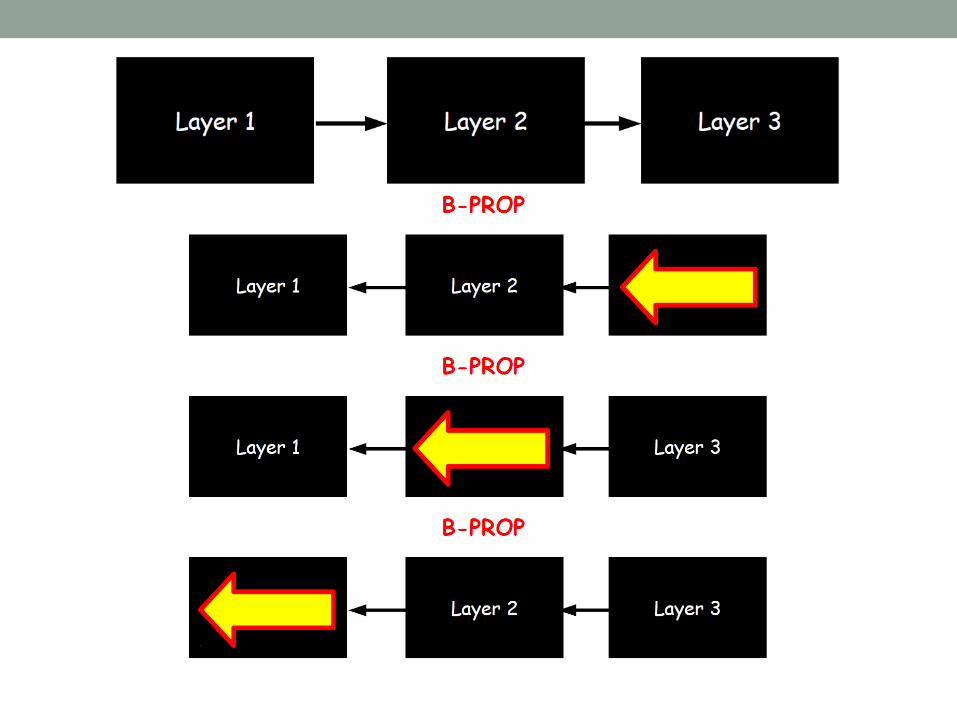
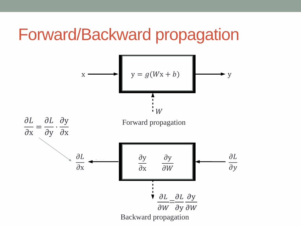
Forward/Backward propagation
Forward propagation
Backward propagation
𝑊
y
𝜕𝐿
𝜕𝑦
𝜕𝐿
𝜕x
𝜕𝐿
𝜕𝑊=𝜕𝐿
𝜕y
𝜕y
𝜕𝑊
y = 𝑔(𝑊x + 𝑏)
𝜕y
𝜕x
𝜕y
𝜕𝑊
𝜕𝐿
𝜕x=
𝜕𝐿
𝜕y⋅𝜕y
𝜕x
x
FEED-FORWARD NEURAL
NETWORK (예시)
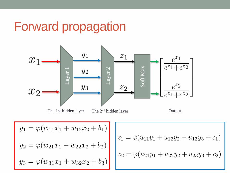
Forward propagation
The 1st hidden layer The 2nd hidden layer
Soft
Max
Lay
er 1
Lay
er 2
Output
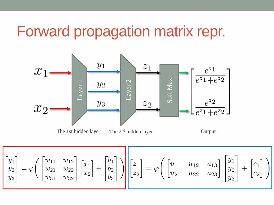
Forward propagation matrix repr.
The 1st hidden layer The 2nd hidden layer
Soft
Max
Lay
er 1
Lay
er 2
Output

BACK-PROPAGATION
ALGORITHM (예시)

Forward propagation
(block-based representation)
Output
Soft
Max
Layer 1
Layer 1
Layer 2
Layer 2

Backward propagation; 2nd layer
Ground
Truth
VS
Output
Soft
Max
Layer 1 Layer 2
• Error propagation

Backward propagation; 2nd layer
VS
Ground
Truth
VS
Output
Soft
Max
Layer 1 Layer 2
• Error propagation

Backward propagation; 2nd layer
• Weight update• Error propagation
Ground
Truth
VS
Output
Soft
Max
Layer 1 Layer 2

Backward propagation; 1st layer
• Error propagation
Ground
Truth
VS
Output
Soft
Max
Layer 1 Layer 2
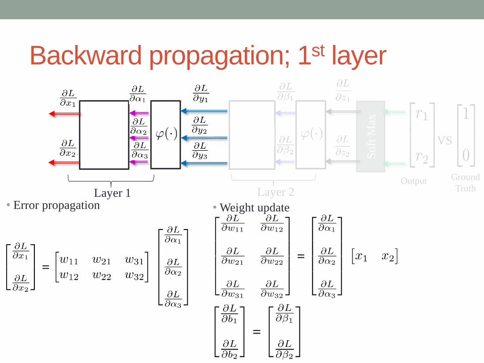
Backward propagation; 1st layer
• Error propagation
Ground
Truth
VS
Output
Soft
Max
Layer 1 Layer 2
• Weight update

TENSORFLOW실습

TENSORFLOW INTRODUCTION

What is TensorFlow?
• TensorFlow is a deep learning library open-sourced by Google.
• TensorFlow provides primitives for defining functions on
tensors and automatically computing their derivatives.
• Tensor is a multidimensional array of numbers
Design Choice
• Network structures
• The mathematical relationship between inputs and outputs
• Loss function
• Optimization
• Optimization methods
• Hyper-parameters (Batch size, Learning rate, … )

Classification vs RegressionClassification Regression
?Expected
Price
1600 sq ft
Color
Weight
Apple
Orange
?
The variable we are trying to predict is
DISCRETE
The variable we are trying to predict is
CONTINUOUS
Housing
Prices

MNIST dataset (classification example)
• handwritten digits
• a training set of 60,000 examples
• 28x28 images


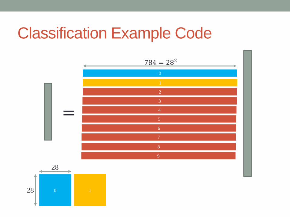
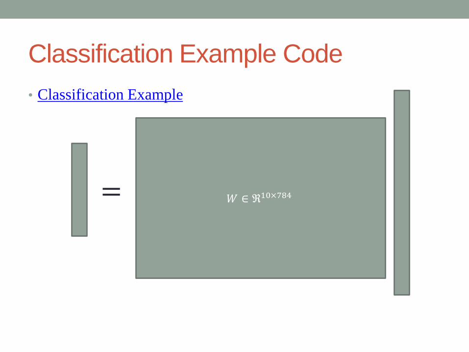
Classification Example Code
=
0
0
1
2
3
4
5
6
7
8
9
1
784 = 282
28
28

VALIDATION
Tasks
ADAS
Self Driving
Localizati
onPerception
Planning/
Control
Driver
state
Vehicle
Diagnosis
Smart
factory
Meth
od
s
Trad
ition
al
Non-machine LearningGPS,
SLAM
Optimal
control
Mach
ine-L
earnin
gb
ased m
etho
d
Su
perv
ised
MLPPedestrian
detection(HOG+SVM)
Deep
-Learn
ing
based
CNN
Detection/
Segmentat
ion/Classif
ication
End-to-
end
Learning
RNN
(LSTM)
Dry/wet
road
classificati
on
End-to-
end
Learning
DNN
Reinforcement
Unsupervised
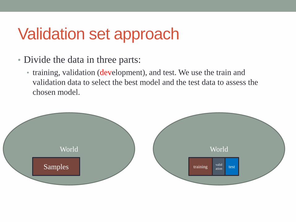
Validation set approach
• Divide the data in three parts:
• training, validation (development), and test. We use the train and
validation data to select the best model and the test data to assess the
chosen model.
WorldWorld
Samples trainingvalid
ation test
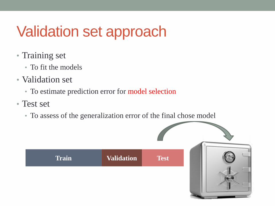
Validation set approach
• Training set
• To fit the models
• Validation set
• To estimate prediction error for model selection
• Test set
• To assess of the generalization error of the final chose model
Train Validation Test

k-fold cross validation
• We partition the data into 𝐾 parts. For the 𝑘 −th part, we fit the
model to the other 𝐾 − 1 parts of the data, and calculate the
prediction error of the fitted model when predicting the 𝑘th part
of the data. We do this for 𝑘 = 1,2,⋯ ,𝐾 and combine the 𝐾estimates
𝐾 = 7
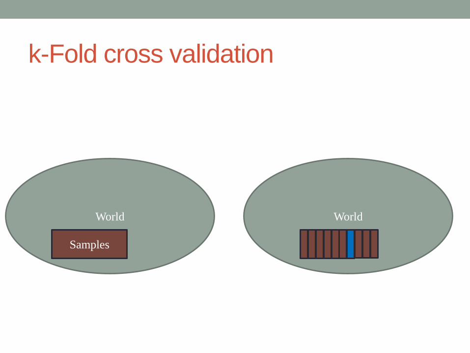
k-Fold cross validation
WorldWorld
Samples
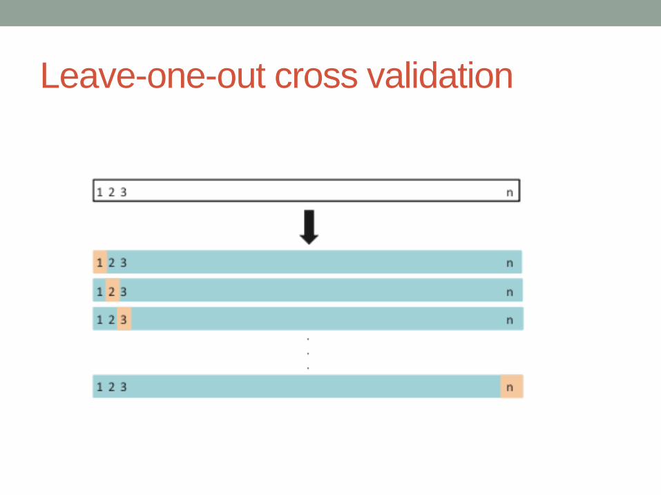
Leave-one-out cross validation

전통적인접근법
Tasks
ADAS
Self Driving
Localizati
onPerception
Planning/
Control
Driver
state
Vehicle
Diagnosis
Smart
factory
Meth
od
s
Trad
ition
al
Non-machine LearningGPS,
SLAM
Optimal
control
Mach
ine-L
earnin
gb
ased m
etho
d
Su
perv
ised
MLPPedestrian
detection(HOG+SVM)
Deep
-Learn
ing
based
CNN
Detection/
Segmentat
ion/Classif
ication
End-to-
end
Learning
RNN
(LSTM)
Dry/wet
road
classificati
on
End-to-
end
Learning
DNN
Reinforcement
Unsupervised

Conventional approach
• Image classification
“Motocycle”
Slides from “Andrew Ng”

Why is this hard?
Slides from “Andrew Ng”

Feature representation
Slides from “Andrew Ng”
Classification
Algorithm
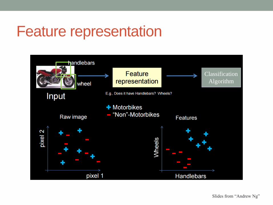
Feature representation
Classification
Algorithm
Slides from “Andrew Ng”
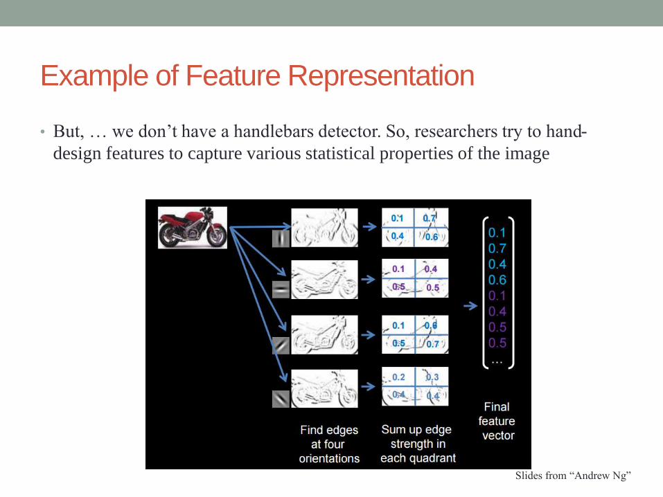
Example of Feature Representation
• But, … we don’t have a handlebars detector. So, researchers try to hand-
design features to capture various statistical properties of the image
Slides from “Andrew Ng”

Feature representation
Slides from “Andrew Ng”
Classification
Algorithm

Computer vision features
Slides from “Andrew Ng”

Audio features
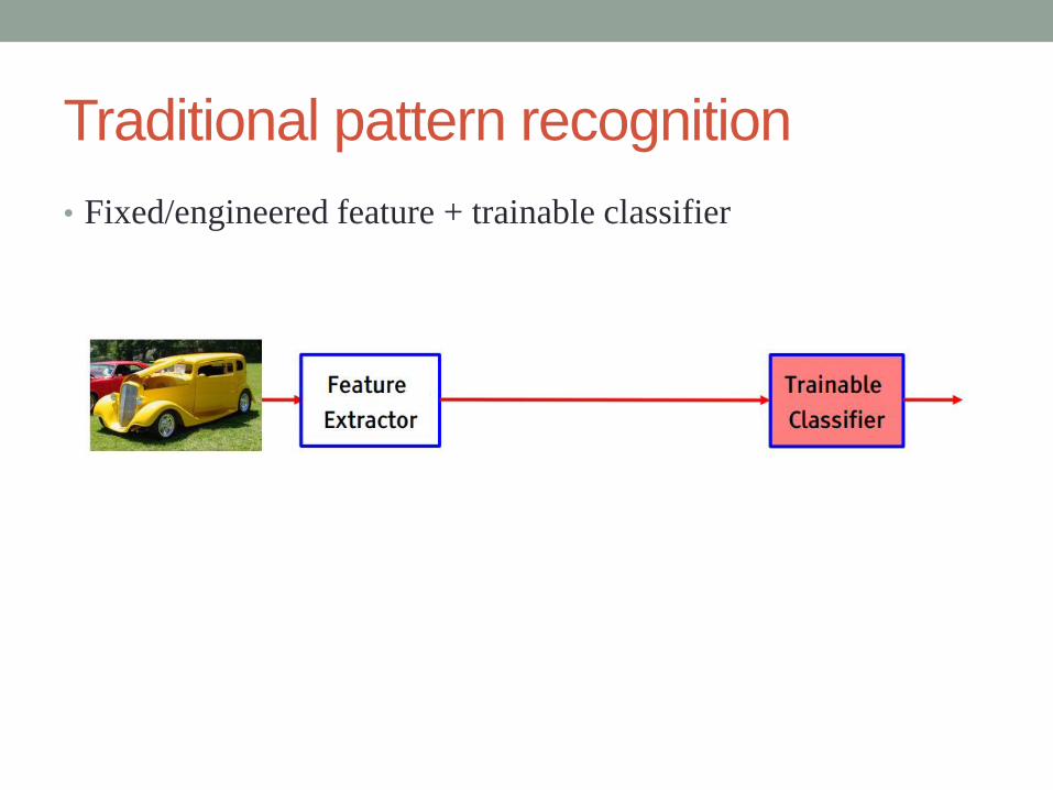
Traditional pattern recognition
• Fixed/engineered feature + trainable classifier
CASE STUDY:
PEDESTRIAN DETECTOR
Tasks
ADAS
Self Driving
Localizati
onPerception
Planning/
Control
Driver
state
Vehicle
Diagnosis
Smart
factory
Meth
od
s
Trad
ition
al
Non-machine LearningGPS,
SLAM
Optimal
control
Mach
ine-L
earnin
gb
ased m
etho
d
Su
perv
ised
MLPPedestrian
detection(HOG+SVM)
Deep
-Learn
ing
based
CNN
Detection/
Segmentat
ion/Classif
ication
End-to-
end
Learning
RNN
(LSTM)
Dry/wet
road
classificati
on
End-to-
end
Learning
DNN
Reinforcement
Unsupervised

Detection problem (binary) classification problem
• Sliding window scheme
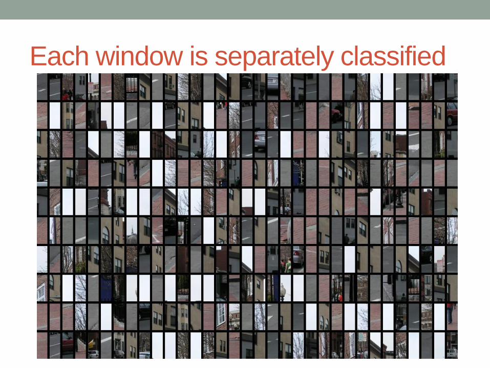
Each window is separately classified

• 64x128 images of humans cropped from a varied set of personal
photos• Positive data – 1239 positive window examples (reflections->2478)
• Negative data – 1218 person-free training photos (12180 patches)
Training data

• A preliminary detector
• Trained with (2478) vs (12180) samples
• Retraining
• With augmented data set
• initial 12180 + hard examples
• Hard examples
• 1218 negative training photos are searched exhaustively for false positive
Training

Feature: histogram of oriented gradients (HOG)
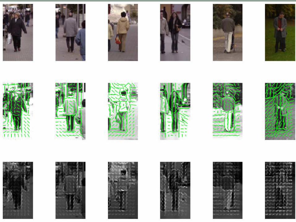
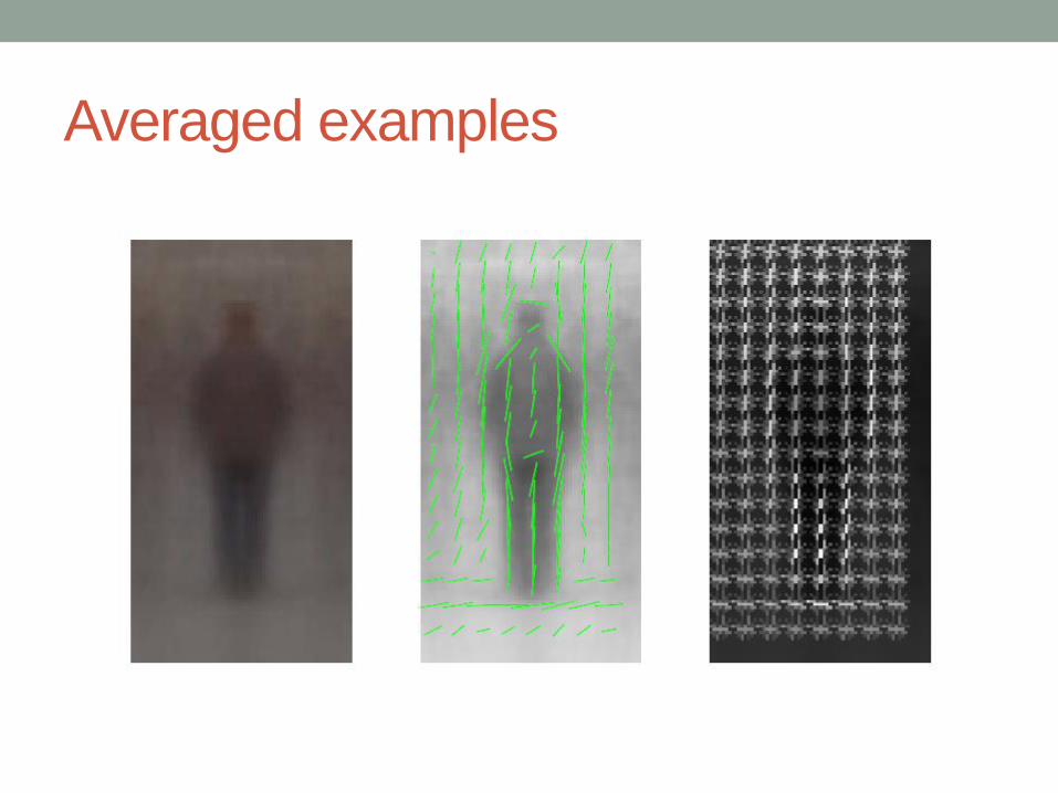
Averaged examples
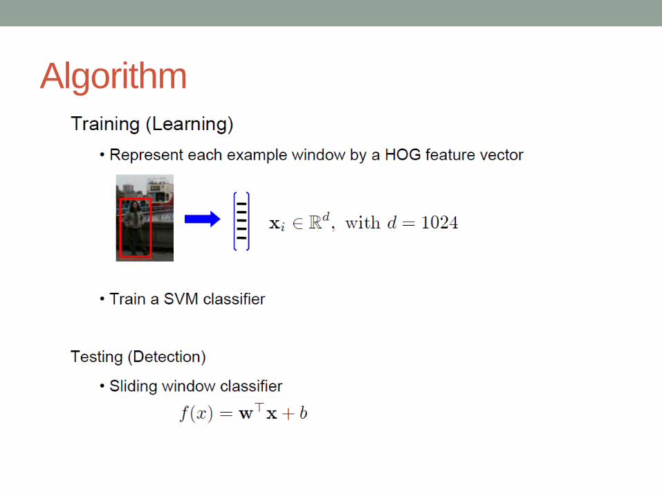
Algorithm

Dalal, Navneet, and Bill Triggs. "Histograms of oriented gradients for human detection." 2005 IEEE Computer Society Conference on
Computer Vision and Pattern Recognition (CVPR'05). Vol. 1. IEEE, 2005.
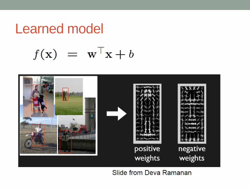
Learned model


![The LovaSz-Softmax Loss: A Tractable Surrogate for the ...openaccess.thecvf.com/...The_LovaSz-Softmax_Loss_CVPR_2018_paper.pdf · the object classes in the dataset [6]. Due to these](https://img.pdfslide.us/doc/110x75/5bd8754f09d3f2740c8c08bb/the-lovasz-softmax-loss-a-tractable-surrogate-for-the-the-object-classes.jpg)


![SphereFace - wyliu.comDeepFace [ FaceNet [ Deep FR [ DeeplD2+ [ DeeplD2+ [ Baidu [ ] Center Face [ 34 Yietal.[ ] Ding et al. [ ] Liu etal.[ ] Softmax Loss Softmax+Contrastive [ 26](https://img.pdfslide.us/doc/110x75/5f5ab075430d5245ae214ced/sphereface-wyliucom-deepface-facenet-deep-fr-deepld2-deepld2-baidu.jpg)