Computer Modelling of Complex Systems with Applications in Physical …doras.dcu.ie/18698/1/Yu_Feng.pdf · 2018-07-19 · 1 Computer Modelling of Complex Systems with Applications

1

Computer Modelling of Complex Systems with Applications in Physical and Related Areas

Y u F e n g B .E n g M .Sc.

Submitted in fulfilment of the requirements for a

Ph D Degree, 1997

School of Computer Applications

Dublin City University

Dublin 9

Supervisor Dr Heather J Ruskin

July 1997

Declaration

I hereby certify that this material, which I now submit for assessment on the programme of study leading to the award of Ph.D. is entirely my own work and has not been taken from the work of others save and to the extent that such work has been cited and acknowledged within the text of my work.

I would like to express my heartfelt gratitude to my supervisor, Dr Heather J Ruskin,

for her supervision, guidance, encouragement and support over the last four years At

every stage of development, she was generous with her time and comments Her faith,

patience and understanding helped make it possible for me to finish

I would like to express my sincere thanks to Prof Michael Ryan, for his help whilst I

was studying in the school of Computer Applications Many thanks are also

expressed to Dr David Sinclair, Dr James Power, M r Jim Doyle and Ms Anne

O ’Brien for all the invaluable help they gave me

I would also like to thank all the former and current postgraduates whom I have met

in the computer lab and the Irish girls with whom I have been lived in Cremore

Heights Especially to Sandra Ward, Gary Leeson, and Dara Mahon, who helped me

to know Irish humour and Ireland, improve my English, and have provided much

support, patience and encouragement since I studied here

I would also like to thank my family and relations for all their love, expectation and

encouragement they have shown over the years I would like to thank my Chinese

friends for their help and understanding while I have been away from home

Finally, I would like to thank the school of Computer Applications for providing me

with the opportunity and the funding to undertake this research This has also given

me the opportunity to learn western culture and enjoy my Irish student life style m

Dublin

Acknowledgements

Abstract

Computational modelling techniques have been applied in physics, biology and other

fields for decades to investigate the scale-invariant properties in non-equilibrium

complex (many-cell) systems Specific examples have been considered to underpin

the simulation of cellular systems, le sandpiles as simple models of transport

phenomena, and soap froths as models of many-cell cellular networks A number of

characteristic properties have been investigated to explore common features of

complex systems Particularly interesting for the simple sandpile automaton is the

achievement of the critical state through the phenomenon known as self-organised

criticality (SOC)

Various simulation algorithms e g cellular automata, direct simulation and Monte

Carlo have been used to model the sandpile and froth systems respectively The

studies of a directed and dissipative C M L sandpile model provide evidence for the

occurrence of SOC, with the system characterised by simple power-law distributions

For the soap froth model, the effect on the evolution of the presence of defects is

investigated, together with the impressions of varying the amount of disorder Scaling

properties obtained, for various initial conditions, are given in detail The

improvements on methods of computational modelling, and the limitations of

software and hardware implementation are also briefly discussed

Table of Contents

1 1 Brief Review of "Cellular" Systems 1

1 2 Type of Systems and Applications 1

1 3 Computational Modelling Techniques 2

1 4 Scope of Thesis 4

Chapter 2 Computational Science (Scientific Computing) and Simulation Techniques 6

2 1 Introduction 7

2 11 Computational Science / Scientific Computing 7

2 12 Model, System, and Simulation 7

2 13 Computational Model 9

2 1 4 Complex (Many-body) Systems 10

2 15 Why do we Need Computer Simulation^ 11

2 2 Computing Environment 12

2 2 1 Hardware Capability 12

2 2 11 Overview on Architecture Principles 12

2 2 12 Storage and Parallelism 13

2 2 13 Parallel Architectures .. 14

2 2 14 Dedicated Machmes 15

2 2 2 Machine Performance—an Illustration 16

2 2 3 Current software Techniques for Handling Updating 17

2 2 3 1 Algorithm Requirements 17

2 2 3 2 Updating Algorithms Sequential Updating 17

2 2 3 3 Simultaneous (Parallel) Updating 18

2 2 3 4 Language Compilation 19

2 3 Simulations for Complex Systems 20

2 3 1 Simulation Classifications 20

2 3 11 Discrete and Continuous Models 20

2 3 12 Stochastic and Deterministic System Problems 21

Chapter 1 Introduction to the Nature of Complex Systems 1

I

2 3 13 Equilibrium and Dissipative Systems 22

2 3 2 Direct and Indirect Simulation Methods 22

2 3 3 Cellular Automata, Monte Carlo and Molecular Dynamics 24

2 4 Simulation Techniques Cellular Automata 25

2 4 1 Cellular Automata Description of Mechanism 25

2 4 2 Background 27

2 4 3 Classification 28

2 4 4 Applications ( 29aT

2 5 Simulation Techniques Monte Carlo 30

2 5 1 Introduction 30

2 5 2 General Principles of the M C Methods 31

2 5 3 Metropolis Method 32

2 5 4 Applications 32

2 6 Other Simulation Techniques e g Molecular Dynamics 33

2 6 1 Introduction 33

2 6 2 Applications . ( 34

2 6 3 Monte Carlo and Molecular Dynamics 35

2 7 Applications of Simulation Methods- Specific Cases 36

2 7 1 CA Models and the Phenomenon of SOC Building Piles of Sand 36

2 7 2 Cellular Networks, Froth Evolutionary Behaviour 37

2 8 Summary ; 38

Chapter 3 Simple Dynamical Cellular System Models 39

3 1 Simple Cellular Automata System and SOC 39

3 11 Simple Cellular Systems 39

3 12 Models and Applications 40

3 13 Scale-Invariance and Self-Organised Criticality (SOC) 41

3 2 Sandpile Automata and SOC 43

3 2 1 Basic Sandpile Driven Model 43

3 2 11 Discrete Driven Models 43

3 2 12 Catalogue of Sandpile Models 47

u

3 2 2 Current Studies on Sandpile and SOC 48

3 2 2 1 Theoretical Results 48

3 2 2 2 Experimental Results 49

3 2 2 3 Computer Simulation Results 51

3 3 Studies of Sandpile Models 51

3 3 1 Simple Sandpile Height Models and SOC .. 51

3 3 2 Results and Conclusions 52

3 3 3 The Directed Sandpile Model with Holes Introduction for a Preliminary

Note 54

3 4 Dissipative Sandpile Models 57

3 4 1 Nonconservative Sandpile Model 57

3 4 2 Various Dissipative Models 58

3 4 2 1 BTW and Zhang Dissipative Models 58

3 4 2 2 CA and C M L Dissipative Models „ 59

3 4 3 Results for CA and CM L Models 60

3 4 3 1 Dissipative Sandpile, CA Model 60

3 4 3 2 Dissipative Sandpile, CM L Models 61

3 4 3 3 Conclusion 64

3 5 SOC and Complex Systems 65

3 6 In Summary 66

Chapter 4 Cellular Network Models 68

41 Background and Introduction . 68

4 11 Cellular Structures 68

4 1 1 1 Introduction 70

4 1 1 2 History 71

4 1 2 Applications Soap Froth Model 71

4 12 1 Basic Geometrical Relations and Topological Processes 73

4 12 2 Von Neumann’s Law and Scaling State 74

4 12 3 Lewis and Aboav-Weaire Laws 75

4 12 4 Simple Soap Froth Model 76

in

4 2 Current Studies of Froths 76

4 2 1 Experimental Studies and Results 77

4 2 2 Theoretical Results 79

4 2 3 Computer Simulation Algorithms and Early Results 80

4 2 3 1 Direct Simulation , 80

4 2 3 2 Monte Carlo Method 83

4 2 3 3 Topological Analysis (Vertex Model) 84

4 2 3 4 The Potts model 85

4 3 2D Froth Models- Implementations via Direct Simulation Methods 86

4 3 1 2D Froth with Voronoi Network . 86

4 3 11 Voronoi Network 86

4 3 12 Voronoi Froth Models- Large Scale Systems 87

4 3 2 Defective 2D Froth Models The Simple Case 88

4 3 2 1 Ordered and Disordered Froth 88

4 3 2 2 Single Defect 2D Froth Model 90

4 3 3 Multiple Defects in an Ordered / Disordered Froth 92

4 3 3 1 Multiple Defects in an Ordered Froth 92

4 3 3 2 Multiple Defects in a Disordered Froth 92

4 4 Results and Discussion 95

4 4 1 Voronoi Disordered Froth 95

4 4 11 Additional Notes on Direct Simulation Implementation- Performance 95

4 4 12 Results of Froth Simulation 96

4 4 2 Froth with a Single Defect 98

4 4 3 Monodisperse and Polydisperse 104

4 4 3 1 Results and Discussion 104

4 4 3 2 Conclusions on Single/Multiple Defect(s) 112

4 4 4 A Note on Stages of Evolution in a 2-D Froth 113

Chapter 5 M C Simulations and other Considerations 119

5 1 System Simulation with M C Introduction 119

5 11 Simple Systems ................................ 120

IV

)

i

5 12 M C for Froths General Points 120

5 13 Implementation for 2D Froth 121

5 14 Froth Coarsening 124

5 14 1 Notes by M C 123

5 14 2 Performance under Different Choices for <A> and X- 126

5 14 3 Performance of Bubble Area 127

5 1 4 4 Summary 129

5 15 Technical Implications of 3D Froth 130

5 15 1 Theoretical Implication 130

5 1 5 2 Technical Implications for Froth by M C Method u 134

5 2 Other Techniques 136

5 2 1 CA for Grain Growth 136

5 2 2 Molecular Dynamics on Wet Foam 138

5 3 Computer Simulation Implementation 138

5 3 1 Simulation Approaches 138

5 3 2 Languages Requirement 149

5 3 3 Algorithms Limitation 140

5 3 4 Limitation of Simulation Methods 141

Chapter 6 Conclusions and Comments 143

6 1 Introduction 143

6 2 Techniques Implementation 143

6 3 Cellular systems and Phenomena Exhibited 146

6 3 1 SOC and Simple Systems 146

6 3 2 Cellular Networks 147

6 3 3 Common Features . 148

6 4 Suggestions for FutureWork 149

References 152

v

Chapter 1 Introduction to the Nature of Complex Systems

1.1 Brief Review of "Cellular" Systems V

Traditional mathematics offers few methods for building a comprehensive theory of

complex dynamical systems A broad research program to study such systems

grows naturally out of studies on complex (many-cell) systems The prototypical

examples are cellular automata and random cellular networks, that appear to be

analytically less tractable Studies of these systems lead naturally to consideration

of the geometry of the systems’ parameter space and the effects of parameter

changes on system behaviour

Cellular Automata were invented by John Von Neumann (1966), who was

interested in connections between biology and the new science of computational

devices, 1 e automata theory This was pursued by the mathematician Stamslaw

Ulam, who suggested using cellular automata as a framework to solve self

reproduction problems, (Burks (1966)) The Game of Life \yas created by John

Horton Conway to demonstrate universal computation in cellular automata,

(Berlekamp et al (1982)) Attention has been attracted to the Game of Life and its

relation to some scientific problems, Poundstone (1985), and in this context

Wolfram (1984) (1986) proposed a classification of cellular automata A

characteristic feature of these cellular automata systems is that they consist of large

numbers of simple identical "units" with local interaction For a review, see

Gutowitz (1990), Mitchell (1996)

Materials consisting of cellular network structures such as metal grains and

biological tissues are common in nature, where the surface energy of the

boundaries makes the pattern unstable, causing certain grains to shrink and

eventually to disappear, Weaire and Rivier (1984) In cellular network systems,

individual interaction has a strong influence not only on its near-neighbours and

next-neighbours, but extending to all the individuals within,the system For a

review, see Glazier and Weaire (1992), Stavans (1993)

1

The study of cellular systems in nature has been a major subject in physical,

chemical, biological and related sciences over decades Its applications cover a

wide range of phenomena and may broadly include, but are not limited to

• Simple cellular systems e g model of transport phenomena, earthquake

occurrences, traffic jam, forest fire, spin glasses, turbulence, Biological

evolution and ecological balance, simple epidemic models, immunological

reactions models and financial market fluctuations

• Cellular networks e g structure and evolution of froths and foams, modelling

of polycrystalline alloys, ceramics structures and lipid monolayers, gram

growth problems and physics of garnet films

In most cases, the simple cellular system is defined as a lattice in position space

Sites may represent points in a crystal lattice, with values given by some quantifiedi

observable or corresponding to types of units The sandpile model, the dynamical

Ising model and other lattice spin systems are simple types of such single cellular

automata system models Many share the characteristic behaviour of Self-j

organised Cnticality (SOC), a concept introduced to describe the process of

achieving a critical state through dynamic adjustments intrinsic to the system as

opposed to governed by an external parameter, Bak (1996)

We concentrate predominantly on simulations of physical and related systems,

where a satisfactory "run" requires the computation of billions of events to

describe formation, growth or evolution While both experimental and theoretical

methods offer basic approaches to understanding complex phenomena, some

systems are difficult to characterise precisely because they are of large size and

involve complex interactions Experimental work is typically difficult to perform,

due to the many parameters involved and theoretical solutions are similarly not

usually feasible or are limited to extreme or equilibrium behaviour for simplified or

approximated systems The rapid growth in power and availability of modern

computers means that, in a simulation, the size of the system may be varied and

1.2 Type of Systems and Applications

2

complex interactions controlled with relative ease This not only serves to

stimulate experimental work and develop new insights to the theoretical system,

but also provides a means of filling the gap between them, Heermann (1990)

1.3 Computational Modelling Techniques

The interdisciplinary area of computational science has grown from the recognition

that physics, chemistry, biology and related fields have a common need for efficient

algorithms, together with sophisticated hardware and software to address complex

problems, Wilson (1987) Simulation techniques form one of the most important

tools in computational modelling and can be used to study i?a diverse range of

phenomena

Computational modelling can be used in a variety of different ways The

traditional methods of direct simulation solve equations numerically in a

straightforward way, providing a direct computer analogue of the physical system

under study Examples are discussed e g by Koonin and Meredith (1990), and by

Gould and Tobochmk (1996) More recently, simplified computational models and

indirect simulations have been used more extensively, where those include

enhancements of early Monte Carlo methods, (based on hypothetical statistical

populations), direct modelling of discrete system elements (using e g cellular

automata), modelling of system interactions through molecular dynamics

simulations, neural network, and other augmented techniques such as genetic

algorithms and so on Recent references include Wolfram (1983) (1986), Jam* f

(1992), Gaylord and Wellm (1995), Frankel and Smit (1996), Crandall (1996) and

Giordanc (1997)

The choice of methods is clearly wide and simulations have been applied m many

research fields The choice of a particular method depends both on the details of

the system and the information sought, but also on practical limitations, smce the

more detail retamed on the system, the more all the demands made of the

simulation Physicists may wish to provide analogies to the behaviour of non

linear dynamical systems and to explam the complex natural phenomena,

computer engmeers may desire to improve the power of a given device; biologists

may wish to model the spread of an epidemic or assess macroscopic behaviour

3

from studies of molecular dynamics and so on, nevertheless the principles of such

simulations remain the same

Specific examples focussed on in this thesis, to underpin the simulation of cellular

systems, are the sandpile automaton and the 2D soap froth, which provide simple

models of complexity with different interaction features and system constraints

These also provide idealised models for a number of more sophisticated

applications and as such, merit attention both in their own right and for the insight

they afford Furthermore scale-invariance in non-equilibrium complex systems is

common and the sandpile automaton as a paradigm for SOC provides a means of

investigating this property through numerical simulations Implementation details

of the different simulation approaches are discussed in the context of these real

problems

1.4 Scope of Thesis :

The arrangement of the material in this thesis is as follows

Chapter 2 defines what is meant by a simulation and why we need to use computer

simulation to deal with complex systems The various categories of simulation

methods are described and distinguished, e g cellular automata, Monte Carlo and

Molecular Dynamics

Chapter 3 reviews the cellular automata method applied to scientific systems

Sandpile models and the phenomenon of self-orgainsed criticality, (SOC), are

discussed in this context Numerical simulations of a directed sandpile model and

dissipative sandpile models are analysed and reported with simulation statistics

used to provide evidence of the occurrence of SOC

Chapter 4 focuses on a model for 2D froth, exploring via direct simulation, the

effect on froth evolution of the presence of defects, large amounts of disorder and

so on The strengths of the direct method are discussed in some detail, together

4

with practical considerations for extending the size of the systems investigated

where a large amount of information on the system structure must be retained

Chapter 5 discusses further the increase in complexity involved in simulating a real

network and considers alternative modelling technique Hardware and software

limitations are considered briefly, together with the improvements which might

reasonably be expected through upgrading

Chapter 6, in the final chapter, we comment on some of the implications for

simulating complex physical systems A synopsis of system type, methodology and

performance is given and recommendations for further methodological studies and

improvement are made, together with suggestions for extending work on the

problems considered at relatively low computational expense

References and appendices are given at the end of the thesis, where the latter

include copies of published papers, algorithm details, detailed figures and a table of

example statistics of froth evolution and a diskette containing full details of the

programmes used

5

Chapter 2 Computational Science (Scientific Computing) and Simulation Techniques

Scientific problems nowadays are not solved solely by the means of conventional

experiments and theoretical considerations A major new ingredient is the use of

computers to aid research It is well-known that physics, chemistry, medicine,

astronomy and other sciences share a common need for efficient algorithms, system

software, and computer architecture to address large computational problems A

new interdisciplinary science, computational science (or scientific computing), which is focused on using computers to analyse scientific problems has been

devised to meet the need and has attracted much attention, Wilson (1986) and

references therein Simulation techniques have played and continue to play an

important role in computational science studies

Simulation is a process which allows us to understand the behaviour of an existing

or potential system by observing the behaviour of a model representing the system

With the advance of simulation approaches in recent years, it provides increased

efficiency in implementation of a complex system without actually constructing or

physically dealing with the system itself A ll the old investigation problems and

some completely new concepts, such as the fractal behaviour of nature are now

studied through computer simulation techniques The applications include a diverse

array of phenomena, in fields ranging from physics and other natural sciences, from

meteorology to social, arts, political and economic processes

In this chapter, we first introduce the notion of computational science and its

components model, system, and simulation Then, we categorise the simulation

classification and discuss simulation as a methodology for focusing predominantly

on the application to complex physical and related systems We present the

architecture needed and distinctive features of the software and describe various

types of simulation techniques and their applicability A discussion of the

underlying theoretical basis for the different techniques is also given in general

terms Specific details are developed for the problems of interest in subsequent

chapters.

6

2.1 Introduction

2.1.1 Computational Science / Scientific ComputingComputational science relates to the knowledge and techniques required to

perform computer simulations and other computationally intensive problems

through model analysis in the respective disciplines, Wilson (1986) Its

characteristics include

• having a precise mathematical statement,

• being intractable by traditional methods,

• having a significant scope,

• requiring an in-depth knowledge of science, engineering (or the arts)

Thus, computational science, involving mixed areas of an applied discipline, seeks

to obtain an improved understanding of some complex phenomena through the

implementation of the problem by a suitable computer architecture and algorithms

In short, it means to investigate a complicated system by an appropriate

computational model usually via computer simulation Various research fields, e g

biology, physics, economics, have established branches of scientific computing

endeavour and have emerged as recognised topics in computational science

Unfortunately, the computer science community has been slow to meet this

development, so that redundancy of effort has ensued

The use of simulation in research and development is now established as a third

basic methodology, complementing traditional theory and experimentation, Decker

and Johnson (1993) The importance of simulation is illustrated by results achieved

for fundamental problems in science and engineering that could be advanced only

by applying computational techniques Some examples include global climate

modelling, turbulence, and biomolecular modelling, Wilson (1987) A detailed

description follows of what is involved in simulation of a system

2.1.2 Model, System, and SimulationThe application of modelling techniques for analysis of system dynamics is a

popular methodological approach in various areas For the solution and flexible

7

application of such models, simulation is of increasing importance. It has been

defined by Naylor et al (1986)

“Simulation is a technique for conducting experiments on a digital computer, this

technique involves certain types of mathematical and logical models that describe

the behaviour of business, economic, physical or chemical systems or some

component thereof over periods of time ”

In general terms, simulation is a form of experimentation that involves asking

decisions in a simulated environment - a laboratory setting that replaces real world

conditions In scientific terms, simulation refers to the process of designing a

model of a real system and conducting experiments with the model for a better

understanding of the behaviour of the system, or evaluating various patterns for the

operation of the system, Bratley et al (1983), Fishwick (1995)

Here, a system can be defined as the understanding of the relationship between

things which interact For example, a pile of sand is a system, in which grains

interact based upon how they are piled I f the pile is unbalanced, the interaction

results in movement of the grams until they find a new condition under which they

are m balance, (either dynamic or static) Isolated groups of sands which do not

touch one another are not a system, because there is no mteraction

A system can be modelled, le one can create another system that supposedly

replicates the behaviour of the original system Theoretically, eg it is assumed that

if conditions for a second group of sand grams replicate the first set, then, we can

predict that they will achieve a new configuration that is the same as the first one

Alternatively, we can use the mathematical representation of sand grams by

appropriate laws, to predict how future piles of the same or different types of sand

will mteract Mathematical modelling is thus fundamental to the description of

system behaviour

A model is therefore, a simplified representation or description of the real system

mtended to be understood As some complex systems may be beyond our intuitive

knowledge, we seek to study and analyse the real thing by constructmg models In

most areas of science and engineering, physical laws are applied to obtam

mathematical models for analysmg systems Model building is relatively easy if the

physical laws are known and the system is compact and well-behaved However,

the modelling of complex, large-scale systems is difficult since many procedural

elements can not be described directly Simulation approaches are used to

overcome these difficulties

Generally speaking, simulation modelling assumes that a system is computable

Here a system is characterised by a number of variables, where each variable value

represents a unique state of the system The dynamic behaviour of the system isi,

observed under different states Thus, the outstanding advantage of simulation is

not only to fully obtain the system’s variability and sensitivity with changing

conditions, but also to increase its safety and productivity Furthermore, whenever

results obtained by simulation modelling are different from those obtained by other

methods, it is the only approach that allows a re-test of system behaviour

Therefore, it is capable of providing insight into aspects of transient misbehaviour,

such as temporary influences by external constraints, which is not available for any

other techniques

2.1.3 Computational ModelA computational model of some process is, essentially, no more than a computer

program It is a program for which claims are made, DeVries (1994) The

structure of the program reflects that of the mechanisms assumed by theory for

the process under study A computational model may be a mechanistic model, or

an input/output functional model, or both Observation of a particular model’s

behaviour can provide precise information on the long-term effects of the system

Thus, computational models can be a source of significant insights for other

similar systems as a new methodology to deal with complex systems

A computational model can also be very effective at driving theory development

Usually, it is not the case that a written program for a model is based on a well-

understood or completely perfect theory However, by exploring computational

variants, the theoretical details can be developed to a deep level, which otherwise

is unattainable For example, Partidge et al (1984) used a computational model to

refute a widely-held theoretical belief, and hence presented a revision of the

acceptance of a class of theories of habitation behaviour.

9

Complex systems span physical science, mathematics, computation and biology In

general terms, a complex system is defined as a network of interacting objects,

agents, elements or processes that exhibit a dynamic, aggregate behaviour,

Bonabeau and Theraulaz (1994) The action of an object possibly affects

subsequent actions of other objects in the network, so that the action of the whole

is more than simple sum of the actions of its parts In other words, a system is

complex if it is not reducible to a few degrees of freedom by statistical description,

1 e forms a so-called many-body system

For instance, a sandpile can be built in the process of adding grams of sand into a

pile With the sand slides become bigger, the pile becomes steeper, and eventually,

some of grams topple till they fall out of the boundary At this point, the system is

far away from equilibrium, and its behaviour and properties can no longer be

understood in terms of those of the individual grams The sandpile generates a

new dynamic, which can be mvestigated through the whole pile rather than every

smgle gram Therefore, the sandpile is a complex system

In general, we are mterested m predictmg, both qualitatively and quantitatively,

the behaviour of a complex system by means of a few relevant physical elements

It is assumed that a large number of mdependent agents are mteractmg with each

other in many different ways Accordingly, system function may reflect various

relationships between them, e g the billions of interconnected neurones make up a

bram Waldrop (1992) has pomted to four aspects of systems which characterise

complexity

1 Systemic mteractions can lead the system to spontaneous self-organisation

2 Complex systems do not just respond to events For example, recent research

has found that species m biology evolve for better survival m a changmg

environment

3 Distinction between complicated and unpredictable Complexity has its

dynamic aspect Every complex, self-organising, adaptive system possess a

kind of dynamism that makes it qualitatively different from static objects, e g

snowflakes, which are merely complicated

2.1.4 Complex (Many-body) Systems

10

4 Complex systems are more spontaneous, disorderly and alive However, their

unusual dynamism may also be far from the unpredictable circuit known as

chaos

It was difficult to study complex system in detail until recent decades because of

the high computational power required For complex systems in any specified

area, the whole system may demonstrate a global dynamic which is not easily

predicted from those of the individual components, thus, much research tends

towards using discrete rather than continuous modelling and corresponding

simulation approaches It is also possible to analyse the behaviour of individuals

based on a large scale network Most investigations are concentrated on

considering the behaviour and properties of interconnected groups

o'*?2.1.5 Why do we Need Computer Simulation?Computer simulation provides a powerful way of solving problems For some

exactly soluble problems, e g in physics, a complete specification of a system’s

microscopic properties leads directly and easily to an explanation of macroscopic

properties One example is that of idealised models like the perfect gas or crystal,

where the Hamiltonian directly gives the state equation, Baxter (1982) In studies

of more complex systems, however, there are no exact solutions available, and in

reality it is too costly to examine every possibility and too difficult to analyse their

behaviour based on a straightforward approximation scheme Computers typically

are used for incidental calculation in this type of work

For scientific problems, the computational aspect becomes more important because

computer simulation has the flavours of both theoretical and experimental features

A good theoretical background is the premise to studying a subject by simulation

methods On the other hand, analytical results do not provide solutions to diverse

problems Pure theoretical approaches tend to be applicable only to very simplified

models Simulations are a useful learning tool for a system under many and varied

conditions, Wagner (1975) eg describes setting up a simulation of a loading dock

with ships moving in and out at specified tides more cheaply and easily than having

the ships physically moving in and out. A forest fire simulation is more easily and

11

less dangerously observed than firing the nearest forest, Ball and Guertm (1992),i

Duarte e ta l (1994)

The results of computer simulations may also be compared with those of theory

and real experiments They provide a test of the underlying model used and,

eventually, if the model is a good one, the simulator hopes to offer insights into the

limitations of theory and experiment to assist the interpretation of new results This

dual role of simulation serves as a bridge between models and theoretical

calculations, and between models and experimental results When dealing with

non-linear phenomena, computer simulation of an idealised model of interest

enables sensitivity analysis via a specified algorithm, Binder (1986) Given this

connecting role, and the way in which simulations are analysed, those techniques

are often called computer experiments as well, Allen and Tildesley (1990)

Furthermore, an important fraction of the human knowledge about critical

phenomena and phase transitions is due to computer simulations performed on

statistical models, Stanley and Ostrowsky (1986) The study of some new research

field, like aggregation phenomena, is wholly based on computer simulation and

experimental data without theoretical understanding to date More details on

computing environments, simulation techniques and applications are discussed in

the next Section

2.2 Computing Environment

2.2.1 Hardware Capability2 2.1.1 Overview on Architecture PrinciplesIn the hardware processing for large scale simulations, it is important to tune the

machine to the needs of the problem being investigated. We consider the structure

of the hardware with respect to storage organisation, processor organisation,

connectivity etc

Vector computers have been used for scientific computing since their development

in the 1970s The first supercomputer architectures included one or a few fastest

available processors to increase the packing density, minimise switching time,

pipeline the system, and apply vector-processing techniques The main task is to

12

repeatedly use a small set of program instructions repeated for multiple data

elements, Hwang (1993) Vector processing has proven to be highly effective for

numerically intensive applications, but not for more commercial uses, such as

online transaction processing or databases

2.2.1.2 Storage and ParallelismIn order to obtain as much memory as possible, it is desirable to introduce a

parallelism concept and construct a parallel approach In general, approaches to

parallelism are classified into the following categories event, geometric, and

algorithmic parallelism, where event parallelism is the most straightforward and

easily applicable

Parallelism has played an important role in computer development in recent years

It is a popular approach for the designers of current supercomputers This

provision in a computer system allows us to utilise the maximum amount of

concurrency and treat the problem with the minimum programming Apart from the

computational power and acceleration of algorithms, parallelism brings with it a

new view on scientific and other processes Generally,^ various levels of

parallelization can be identified These are respectively

(i) Instruction level parallelism which is the heart of all "multispin" coding

algorithms This can turn a normal scalar computer into a mini-parallel computer,

and also provides the basic programming tool for SIM D (Single Instruction

Multiple Data) machines

(u) The chaining level of parallelism, which is closely associated with vector

computers and which typically, can execute a multiplication instruction and an

addition instruction simultaneously More sophisticated machines such as the

CRAY YM P can execute logical and shift operations simultaneously

(in)Parallelism can also be introduced at a higher level in the form of multiple

vector processors which can execute different parts of a loop simultaneously and

spread loops automatically Such systems clearly represent thé emerging trend in* \

supercomputing architecture e.g. CRAY X M Y .

13

The paraUelism approach is considered an appealing one because it can accelerate

the execution of a single program and increase throughput and reliability The

existence of an independent control unit makes possible to execute parallel loops

with branching, subroutine calls and random memory activity as compared to single

processor vector machines which have insufficient computational resources to

handle the complexity of the problems and achieve the accuracy required

2 2.1.3 Parallel ArchitecturesIn the 1980s, the first massively parallel processors began to appear with the single

goal of achieving far greater computational power than vector computers by using

low cost standard processors Theoretical models of parallel computing illustrate a

number of possible parallel computer architectures, but not all of these have

physical realisations The limitation includes the number of processors, their mode

of operation, the memory organisation and the connectivity between the

processors The number of possible combinations is quite large

There are two mam categories of structures on most existing parallel machines On

the one hand, there are machines with a small number of very powerful processors,

similar to the CRAY and Alliant which have only two, four or eight processors On

the other hand, there are machines with a very large number of processors, each of

which is much less powerful and mdeed some of which have only bit-level

capabilities Examples mclude the Connection Machine, Heermann (1991)

A further classification on the various types of machines mclude Smgle Instruction

Multiple Data (S IM D ) and Multiple Instructions Multiple Data (M IM D ) The

instruction of SIM D is broadcasted by an external controller and executed by the

processors This type of architecture is most effective when it can exploit

parallelism at the level of the data on which it operates, this means that the problem

can be solved by simultaneous operation on all of the data elements mvolved The

Connection Machine is an example of SIM D type One of these, the CM -2, is

considered, for example, to be a very good tool for cellular automata simulation

and m addition, provides a useful means of exploiting the natural parallelism of the

spatial grid as well as its capacity to perform efficient communications with

neighbourmg data pomts In terms of the cellular automata example, one of the

14

mam virtues of the CM -2 is that it has a Boolean hypercube configuration which

means that it allows usmg a code indexing scheme to embed multi-dimensional

grids into the hypercube so that nearest neighbours are naturally preserved

Machines such as the CRAY (mentioned previously) have the feature that each of

the powerful processors can operate more or less as a conventional computer

mdependent of the other processors and these thus belong to the M IM D class

2.2.1.4 Dedicated MachinesFor some problems, such as many which arise m statistical physics, the computer

time required for the solution is prohibitively large for a conventional computer

This is an obvious and important reason why we do not use a general purpose

computer but endeavour rather to create special purpose machines is m order to

make best use of the time and substantial computmg power which is available As

an example, agam taken from physical applications, the investigation of the spm

glass problem on a special purpose computer used the equivalent of one year of

CRAY time1

A dedicated machine which can match either the problem itself or the particular

algorithm can be used to solve the problem m a relatively short time Moreover,

the price of a dedicated machine may be cheaper than a conventional one because

although it needs more silicon chips these are mexpensive and readily available

There are several specific machine types that have been tried on cellular automata

smce these were first mtroduced by von Neumann (1951) The first CA machine

was created by Toffoli et al (1981) Designated CAM -6, it provided an array of

256 by 256 locally connected cells, each one with four bits of state The state of

every cell is updated 60 times per second Although it is a sequential machine, its

execution is very fast with a performance comparable to a supercomputer The

cellular computer is used for its computational capacity because it is comparable to

the case for a general-purpose computer In particular its capacity means that it can

be used as an experimental environment for modelling abstract or real physical and

related phenomena

15

The main drawback of this kind of architecture is the increasing, size of the look-up

table For instance, if we have three planes with 9 bits per plane, the look-up table

should store 227A3 bits, 1 e = 50 Mbyte of information

Another dedicated machine is the Reseau d’Automate Programmables 1 (R A P 1),

which is used for modelling fluid dynamic behaviour and cellular networks,

Manneville (1989) Such machines can be considered as simplified versions of the

Connection Machine The disadvantage of a special purpose machine lies in its

inflexibility It is difficult to use it directly for a new system involving new

techniques and modified algorithms

2.2.2 Machine Performance-an IllustrationConsiderations of applications of large-scale simulations on general purpose

machines can be illustrated by a review of the results of implementations of

selected programs on two scalar mainframe machines, a vector, computer, and on a

SIM D and M IM D computer by Kohrrng (1991) The speeds achieved are

described in terms of the MUPS (millions of sites updated per second) This is a

convenient measure of performance, given that such programs typically consist

almost entirely of integer and logical instructions and not of floating point

operations, Kohrrng gives an example of cellular automata On the scalar

computer, SUN Spar-1 and IBM -3090, the MUPS speed was 1 6 and 2 7

alternatively On the CRAY XM P where the individual processor is a high-

performance vector machine, the speed was 233 For the Connection Machine,

CM-2 16(384-processors, SIM D computer), the speed was 270, compared to 1690

on the M IM D computer CRAY YM P/832 8-processors This last is clearly faster

than all others to date and has considerable implications for researchers hoping to

achieve comparable performances on less-sophisticated systems for similar classes

of problems

16

2.2.3.1 Algorithm RequirementsIn large scale simulations of representations of real systems, it is obvious that the

development of the basic hardware has been insufficient, in part because problems

which are challenging in their own right must be solved in order to construct the

machines as well as achieving more computational power Rather than relying on

new hardware developments, therefore, we need to improve the software

techniques so that the hardware can run the simulations with maximum efficiency

given the current provision Furthermore, it is also necessary to develop algorithms

which can be efficiently implemented on a variety of machines with only minor

programming changes We next discuss some algorithms and how these handle the

updating of results in fixed provision hardware

2.2.3.2 Updating Algorithms: Sequential UpdatingMany problems that are of interest in numerical investigations, for example the

solution of systems in statistical physics, require the simulation of a large number

of simple variables, each of which is represented by a small number of bits or single

bits General-purpose computers usually provide complicated operations on long

data words The sequential updating procedure consists of updating the variables,

one by one, in either a random or a prescribed periodic order The simple

implementation of this process can be carried out on any computer with, for

example, a FORTRAN 77, or FORTRAN 90 compiler since all the sites have to be

updated at the same time

It is clear that sequential updating of the code is extremely inefficient The ideal

rule we take should be inherently parallel and simultaneously applied to all the sites

for a complete realisation of the system The obvious failing, therefore, is that this

implementation wastes enormous amounts of memory In this case, it involves ar

large number of useless computations since the CPU operates on overall words

rather than those bits which contain the relevant information The states of the

system are typically binary 0 or 1, thus it is sufficient to use one word for several

bit variables

2.2.3 Current Software Techniques for Handling Updating

17

>/

Parallel dynamics consist in updating all the variables synchronously, where this is

known as the multi-spin or multi-bit coding method It makes an efficient use of

the computer memory and gives some degree of parallelism to the scalar processor Multi-spin coding is an effective approach to implementing large size

simulations of real systems

Many bits are stored in a single computer word so that if e g the word length is 32

bits, we can clearly save 32 one bit variables in one word We can then use a

logical method of counting the neighbouring bits and updating the sites, e g the

logical bitwise EOR and bitwise AND to sum over neighbouring sites It is thus

possible on serial machines to treat several variables at the same time and achieve

partial parallelism Oliveira (1990) has discussed the application of computing

Boolean (only two states) statistical models by Boolean operations AND, OR and

XOR

On vector machines, we can exploit, in part, the inherent parallelism by considering

the data structure The processing of the code requires that we only need to change

the names of the bitwise intrinsic SHIFT and the definitions of left, right and

circular shift functions which may vary on different machines, Stauffer (1991)

However, we can use the bit-by-bit handling functions, where IO R can produce

logical OR operations in parallel The first bit of IO R (N l, N2) is the logical OR of

the first bit of N l and the first bit of N2, the second bit applies similarly to the

second bits of N l and N2 and so on

On M IM D machines, the hardware architecture is different, but can similarly be

used to handle many bits simultaneously and multi-bit coding is applicable For this

reason, the speed of M IM D machines is faster than any others

The advantage of multi-spin or multi-bit coding is clearly that it saves on the

memory and increases the speed by exploiting parallelism and updating each bit on

the whole word For most usual general-purpose machines, best performances are

obtained with vector computers For example, on the CRAY computer, one bit is

used for one spin and 64 bits in a word are updated simultaneously with a speed of

2.2.3.3 Simultaneous (Parallel) Updating

18

340 spin updates per microsecond for the YM P/832 processor for the

hydrodynamic example of Kohring (1991)

2 2.3.4 Language CompilationBoth machine architecture and computer language have considerable influence on

the way in which the user perceives a particular problem and formulates algorithms

to solve it numerically The hardware and the software having been discussed in

general terms, and we now consider the relation between them, i e explore the

potential of the inherent parallelism of the machine together with the encoded

language■a

Traditionally, large amounts of code for scientific and engineering computations

have been written in FORTRAN Unfortunately, it is necessary to adjust the

programs to the compiler one is using due to the fact that different FORTRAN

compilers treat the functions differently and have different organisation of the

memory For example, ISHFT is not yet a standardised FORTRAN function, but is

implemented in some form on most machines ISHFT(N1, N2) shifts the bits of

word N1 by N2 positions to the left or N2 positions to the right when N2 is

negative The rightmost N2 bit positions of N1 should then be filled with zeros or

the leftmost N2 bits when N2 is negative The circular shifts are not available, and

the bit-by-bit functions vary and have different definitions

New FORTRAN versions constantly attempt improvement on this, but the

standardisation of regular functions typically needs a long time to be accepted by

all users This is particularly the case where large elaborate programs have been

constructed and are in use for complex problems, using a given set of functions

However, programs written in other languages such as C and PASCAL, are more

standardised on bit operation and are gradually becoming more widely used in

scientific applications One such is C, which has the advantage that FORTRAN and

C interface very readily and efficiently, so that a FORTRAN program can use C

routines, and vice versa, with little programming effort

19

2.3 Simulations for Complex Systems

2.3.1 Simulation ClassificationsWhen we attempt simulation of a system, similar considerations arise, irrespective

of the nature of the application In what follows, we concentrate on some well-

established simulation approaches and some application areas, in particular of

physical and related many-body complex systems We classify the simulation by the

types of computational models, system characteristics and simulation methods, as

indicated in Section 2 12

2.3 1 1 Discrete and Continuous ModelsModels can be broadly divided into two categories based on the types of system

variables, namely continuous and discrete When the predominant activities of the

system cause smooth changes in the attributes of its entities, the system is

represented by a continuous model I f the system changes occur discontinuously, it

is described as a discrete one, Kaplan and Glass (1995)

Both ordinary and partial differential equations formalism are used to define

simulation models of continuous systems Difference equations, cellular automata,

and Markov chain models are used to specify discrete-time systems, (where time is

represented by integer numbers)

Continuous simulations were traditionally carried out through the medium of

analogue computation, Bennett (1976) With the appearance of the digital

computer in the early sixties, the digital processor was seen to be a superior

simulation tool Further the mathematical modelling of complex systems has in the

past been implemented by various standard programs to solve those ordinary and

partial differential equations The programs are usually written in FORTRAN,

PASCAL and C. Consequently, a researcher with modest modelling needs has had

little option but to produce his own program This has effectively prevented the

development of mathematical models in many areas of scientific research Recently,

several software products have been developed which strip away the veils of

mathematical complexity and provide the modeller with tools, Stauffer et al

(1988)

20

In discrete models, the interactions can in general be viewed as discrete events

undergoing local state changes to neighbours in some space, e.g. calculable by

means of discrete event, object-oriented simulation of collections of subsystems.

The concept of an event driven simulation contains the most general updating

scheme for a simulation, since an event can be either externally or internally

generated. In a special case, an event can be a time step, so a time stepped

simulation is named a discrete event simulation, Vesely(1994).

2.3.1.2 Stochastic and Deterministic System Problems

A deterministic system is referred to as based on a Newtonian vision of cause-

effect as found mostly in physics. Change in the state of a system can occur

continuously over time or at discrete instants in time. The discrete instants can be

established deterministically or stochastically depending on the nature of model

inputs. Systems exhibiting deterministic characteristics are predictable, linear, and

controllable. Therefore, small stimuli cause small outcomes, and large stimuli will

have large outcomes. All the events are ahistoric which means experiences do not

change the result.

The simulation problem is defined to be either probabilistic or deterministic depending on whether or not they are directly concerned with the behaviour and

outcome of random processes. A stochastic model or probabilistic model has at

least one random variable and therefore, at a given instant in time the next state of

the model is not uniquely determined. Deterministic models (also called state-

determined models) are those where the current state and current input, if any,

uniquely determine the next values of state variables, e.g. molecular dynamics,

Heermann (1990).

Although the procedure for describing the dynamic behaviour of discrete and

continuous model changed differ, the basic concept of simulating a system by

portraying the changes in the state of the system over time remains the same.

In a simulation, we usually try to ignore the uncertainties of model in order to treat

the models as deterministic ones if the uncertainties are of little importance

compared with the general behaviour of the model. However, a large class of

21

problems are stochastic in nature Topics such as percolation and Monte Carlo

methods of modelling systems are of this type, Janke (1995)

2.3.1.3 Equilibrium and Dissipative SystemsA system in equilibrium is stable in the sense that while perturbations can move

the system away from stability, at least temporarily, coping mechanisms exist to

restore stability after such a shock In addition, in an equilibrium system, primary

emphasis is placed on the relations among separate components of the systems

under analysis

Dissipative systems abound in complexity theory and involve complicated yet

deterministic interaction between agents These systems are open to environmental

influences and undergo real change and restructuring based on inherent stability

Unlike an equilibrium system, a dissipative system when perturbed will undergo

changes which create a new equilibrium, different from previous points in time

Equilibrium systems, by contrast, show only momentary fluctuations before

settling back into the previous state

Toffler (1984) has discussed how a dissipative system on the edge of chaos

undergoes change He suggested that all systems contain subsystems which are

continually fluctuating At times', a single fluctuation or a combination of those

fluctuations may become so powerful, as a result of positive feedback, that it

shatters the existing organisation However, at this revolutionary moment, which is

designated the singular moment or a bifurcation point by the author, it is

impossible to determine in advance which direction change will take, i e whether

the system will dissipate into chaos or leap to a new, more differentiated, higher

level of order or organisation, called a dissipative structure This phenomenon

contains a very attractive and important question, l e whether disorder arises out

of order or order out of disorder Simulation of a complex system may also

provide some insight to this question for specified systems (see Ch 4)

2.3.2 Direct and Indirect Simulation MethodsDirect simulation methods refer to the simulation of numerical equations in a

straightforward manner to obtain the solution Use of numerical simulation

22

methods include solving linear equations, eigenvalue problems, differential

equations and partial differential equations, and others In the traditional study of

physical and related systems, most applications of computer simulation concentrate

on these methods which describe the underlying system models directly and

provide solutions to the equations that govern the physical processes

A mathematical model is introduced to describe, as for as possible, the physical

system for which a set of assumptions apply which make the solution of the

problem somewhat more tractable The model is essentially an idealised version of

the system and the aim is to obtain parameters of the model which relate directly to

properties of the system that we wish to measure Hence, the simulation

corresponds to reproducing computationally as many of the actual system features

as possible, then recording the effects of change or inducing changes to occur,

where these closely mimic real changes in the system This approach defines so-

called direct simulationHowever, the investigation of non-equilibrium, complex (many-body) systems,

which cannot be described by a set of linear differential equations is subject to

limitations when using the conventional direct simulation approaches No general

solution is known when the number of interacting bodies is greater than two

Useful results are sometimes obtained by making some simplifying approximations,

(e g the simplest one consists of neglecting interactions altogether), or by reducing

the problem to an effective one-body problem. Nevertheless, all known

approximate schemes are of limited applicability Direct simulation meets with

difficulties since equations used to describe the system model are difficult to solve

without further simplifying assumptions or possibly more advanced computing

techniques if available The alternative general approach to handling problems

involving complex many-body dynamics is typically based on discretization of the

system processes, so that these can be broken down into a series of small steps

This principle underlies indirect simulation in that a slightly different problem to

the actual one of interest is actually modelled Such methods rely on reproducing

system properties through either aggregate or ensemble behaviour, rather than

implementing them straightforwardly, Jain (1992), Thompson (1992) Monte Carlo

methods, cellular automata models, molecular dynamics, neural networks and

23

related techniques have become more widely used as indirect simulation

approaches to formal mathematical models, in order to investigate the evolutionary

properties of these complex systems

Indirect methods tend to deal with simpler aspects of a system, and are thus

particularly suitable for problems requiring computation of millions or even billions

of similar types of events, such as e g growth or division of cells in molecular

biology, re-onentation of spin in the Ising model of a ferromagnet, and others,

since the difficulty lies in achieving simulated behaviour which in the limit

approaches that of the real systems Thus a satisfactory run will require the

computation of billions of events to describe formation, growth or evolution Some

illustrations are given subsequently

2.3.3 Cellular Automata, Monte Carlo and Molecular DynamicsCellular automata, Monte Carlo Methods and moleculai dynamics are three

important indirect simulation techniques which are currently enjoying considerable

popularity in the modelling of physical and related complex systems Typically, M C

is unsurprisingly used as a stochastic method, M D as a relatively deterministic one,

whereas CA is used in both ways To distinguish more clearly between the

methods, we have

Cellular automata (CA) form a class of mathematical systems characterised by

discrete local interaction and an inherently parallel form of evolution CA provide

prototypical models for complex processes consisting of a large number of simple

locally connected components Examples of phenomena that have been modelled

using CA include turbulent flow caused by the collisions of fluid molecules, growth

of crystals and patterns of electrical activity in simple neural networks, Wolfram

(1984)(1986) ^

Monte Carlo (M C) is a numerical analysis technique that uses random sampling of

distributions to estimate the solution of physical and mathematical problems, l e it

is roughly one of the statistical simulation methods, Landau (1994)

Molecular Dynamics (M D ) provides the methodology for detailed microscopic

modelling on the molecular scale The system can consist of few or many-bodies,

with the motion of each individual atom or molecule described according to e g a

24

Hamiltonian, (usually describe aggregate energy of a system) M D usually involves

calculations on a number of particles, from a few tens to a few thousands, or even

several millions Macroscopic quantities are extracted from the microscopic

trajectories of particles It is a tool which we can use to understand macroscopic

physics from an atomic point of view The applications of M D include the

thermodynamic properties of gas, liquid, and solid, plasma and electrons, transport

phenomena etc, Haile (1992)

2.4 Simulation Techniques: Cellular Automata

Cellular Automata (CA) is an important area in the field of complexity which is

linking different domains of traditional sciences One main achievement is that CA

focuses on system global phenomena through local simple individual interaction

Such phenomena occur in many fields and at many levels of description, e g ants

interact to form a colony, or water molecules interact to make a fluid, or sandpiles

interact to create avalanches As we discussed in the last section, it is necessary to

choose a simulation model which accurately reflects these aspects of a complex

system that we wish to study Many such systems share the common features

above and CA models, because of their simplicity, have performed well in terms of

representing these Not all systems are best represented by the same type of CA

and there are numerous variants

2.4.1 Cellular Automata: Description of MechanismA cellular automaton (CA) is a discrete dynamical system Space, time and the

states of the system are discrete Each point in a regular spatial lattice, called a cell,

can have any one of a finite number of states The states of the cells in the lattice

are updated according to a local rule That is, the state of a cell at a given time

depends only on its own state at one previous time step, and the states of its nearby

neighbours at the previous time step A ll cells on the lattice are updated

synchronously Thus, the state of the entire lattice advances in discrete time steps

(Gutowitz (1996))

In mathematical terms, a cellular automata is described as a lattice of finite state

automata with N states, and K neighbours for each cell The state S of each cell is

25

updated in discrete time steps as a function of state transitions defined for the

alphabet N K the combination of states for each cell and its neighbours

S(NK)—>S(i) (2 3 1)

one-dimensional CA is an elementary cellular automata with N=2, K=2

S(i-1), S(1), S(1+1) -> S(1) (2 3 2)

Shown in Fig 2 3 1, the neighbourhood of each cell consists of itself and its two

nearest neighbours with periodic boundary conditions The CA rule is often

displayed as a lookup table, or rule table, which lists each possible neighbourhood

together with its output bit, (the update value for the state of the central cell in the

neighbourhood)

Rule table:neighbourhood 000 001 010 011 100 101 110 111

output bit 0 1 1 1 0 1 1 0

Lattice

t=0 10100110010 it= l 11101110111 *

Fig 2 3 1 one-dimensional, binary-state CA with periodic boundary conditions shown

iterating for time step

The behaviour of a CA is often illustrated usmg space-time diagrams m which the

configuration of states m the d-dimensional lattice is plotted as a function of time

Fig 2 3 2 shows the behaviour of a CA with N=200, iterated over 200 time steps

This is a basic CA architecture and it can be modify m many ways, such as for

higher dimensions, different boundary conditions, stochastic rather than

deterministic CA rule and so on

26

0

time

1990 site 199

Fig 2 3 2 a space-time diagram, showing the typical behaviour of CA Cells in state 1 are

displayed as black, and cells in state 0 as white, Mitchell et al (1996)

2.4.2 BackgroundCA were first described by Von Neumann and Ulam, who studied the behaviour of

models of coupled masses and springs, resulting in the first computational evidence

of chaotic behaviour in dynamical systems, Von Neumann (1966) Conway

developed the Game of Life system, which is a simple 2-D analogue of basic

processes in living systems, which is the most widely known example of a CA The

game consists in tracing changes through time in the patterns^ formed by sets of

"living" cells arranged in a 2D grid The rules governing these changes are

designed to mimic population change Wolfram (1984) (1986) was the first to

point out the potential for extensive use of CA models in statistical physics and

later a number of authors, e g Stauffer (1990), developed the links between

physical systems and CA like structures in nature so that numerous biological

examples are now to be found in the physical literature These include e g

immunological and ecological studies For a further review, see Manneville et al

(1989)

27

The essential feature of a cellular automaton lies in the fact that its state variable

takes a different separate value for each cell The state can be either a number or a

property Its neighbourhood is the set of cells that it interacts with So, a CA model

usually is used to describe the system in terms of relations between cells Some

complex systems fit easily and perfectly into the framework of cellular automata,

for others these simplifying assumption are too restrictive for real modelling CA

are used not only as models in natural sciences, but are also appropriate models of

parallel computation features due to their complete space-time and state

discreteness

2.4.3 ClassificationSeveral researchers have been interested in the relationships between the generic

dynamical behaviour of CA and their computational abilities Despite the

computational simplicity of CA, they are capable of a variety of behaviour An

important property is that they tend to be self-organising \ 1 e starting from

complex, random cell configurations, the rules governing the system cause patterns

to occur from initial chaos Wolfram (1984) suggested that CA rules can be

classified into four qualitative classes, based on the space-time pattern

demonstrated by CA at long times

1 Spatio-temporally uniform state The automata reaches a homogeneous state

regardless of initial conditions

2 Separated simple or periodic structures The automata reach a state after some

relatively small transient period consisting of space time separated

configurations The configurations vary in detail depending on the initial

configuration, but may have overall behaviour which is independent of the initial

state

3 Chaotic space-time patterns The automata reach a chaotic evolution pattern

starting from random initial conditions

4 Complex localised structure Properties vary with initial conditions

The disadvantage of Wolfram’s classification is that class membership is

undecidable, Culik and Yu (1988). After Wolfram’s work, several researchers

have queried the relation of static properties of CA rules to their dynamical

28

behaviour Langton (1990) studied the relationship between the average dynamical

behaviour of cellular automata and a particular statistic (A,) of a CA rule table

Langton selected a number of two-dimensional CA samples Starting with A,=0 and

gradually increasing to X.=l- 1/k, he found that the average behaviour of a CA‘ *

undergoes a phase transition from ordered behaviour, which has a fixed or limiting

cycle after a short transient period, to chaotic behaviour As X reaches a critical

value Xc, those rules tend to have longer transient phases Moreover, Langton

indicated that CA close to X tend to exhibit long-kved, complex pattern, 1 e non

periodic, but non-random, where the Xc stage roughly corresponds to Wolfram’s

fourth class of CA For a review of the relationships between X and dynamical and

computational properties of CA, see Mitchell et al (1994)

2.4.4 ApplicationsThe nature of CA is to provide a convenient abstraction of continuous phenomena

Models of this type are thus useful for studying problems of energy transfer and

biological growth pattern, fluid flow, and earthquake evolution, Gutowitz (1990)

The properties being observed normally correspond to patterns that are coherent

over a large array of cells, although the cells are not co-ordinated with a specific

set of cells In simulations, the elemental level of CA allows us to get more

information for the processes occurring within the system This breakdown of the

statistics into detailed structured information is one of the addtional objectives of

the thesis In the most direct cases, the cellular automata lattice is in position space

This sites may represent points in a crystal lattice, with values given by some

quantified observable or corresponding to the types of units The sandpile model,

dynamical Ising model and other lattice spin systems are simple types of CA

models

Furthermore, CA provides a computational and analytical development for general-

purpose ideas on the studies of complex systems, e g Forrest (1990) has used CA

as abstract models to study emergent behaviour These systems are inherently

difficult to analyse due to their complexity. The discreteness of CA is expected to

\

29

make the analysis simpler The ideas can used in generalising more continuous

systems, such as Coupled Map Lattices, which are discrete in time and space, but

have a continuous state variable

Cellular automata can be considered as parallel processing computers The

computational capabilities of CA have been used extensively, Toffih (1987), and it

has been shown that some CA could be used as general purpose computers, and

may therefore, be considered as general paradigms for parallel computation, (as

Turing machines provide a paradigm for serial computation) The local and

uniform nature of the laws governing cellular automata means that a hierarchy of

structures and phenomena may be represented, including operation at molecular

level

2.5 Simulation Techniques: Monte Carlo

2.5.1 IntroductionThe name Monte Carlo was applied to a class of mathematical statistical simulation

methods first used by scientists working on the development of nuclear weapons in

Los Alamos in the 1940s The principle of this method is the invention of games of

chance whose behaviour and outcome can be viewed as relating to competition and

evolutionary behaviour in real world systems The effectiveness of numerical or

simulated gambling as a research effort was developed by digital computer, (e g

Kalos and Whitlock (1986) for commentary), where, in particular, these simulation

deal with a large number of chances or events The treatment of the probability of

event occurrence, the aggregation of results and their statistical analysis together

with methods of dealing with bias and errors are all core features of the M C

approach

Statistical methods are then used to obtain microscopic properties from averages of

mechanical variables of molecules The Monte Carlo (M C) method is defined by

representing the solution of a problem as a parameter of a hypothetical population,

and using a random sequence of numbers to construct a sample of the population,

from which statistical estimates of the parameter can be obtained, Binder (1986)

30

M C methods are thus stochastic rather than deterministic procedures, where atoms

are moved more or less randomly during the course of the simulation In M C, a

number of molecules (or ions) are confined within a region, then at each step, a

randomly chosen molecule is moved to a new randomly determined location The

computer then determines whether to accept or reject this movement depending on

whether the energy change of the resulting system state is acceptable according to

some predetermined criterion This process is repeated many times until there is no

further change in the energy and other captured properties of the system, at which

point the system is deemed to have a reached thermodynamic equilibrium Usually,

a large number of molecular states are generated and the corresponding physical

properties of these states are averaged to obtain macroscopic properties of the

system, such as energy and entropy, Binder (1992)

2.5.2 General Principles of the MC MethodsThe random nature of a Monte Carlo simulation means that, in the long run, the

simulation will approach equilibrium values, while an individual move has a

realistic chance of taking the simulation away from equilibrium As M C typically

uses pseudo random number generators to generate the element of chance, its

applications are enormous and provide insight in many fields Many problems,

which at first glance do not seem to fit the M C criteria, can have behaviour which

is related to some stochastic element of the system to which a solution is sought

M C can be considered in either direct or indirect terms The direct application, is

less commonly used but as would be expected, concentrates on a straightforward

simulation of the original problem It relies on the numerical solution of equations

defining the system, which can be used to predict the model properties at different

stages Indirect methods solve a related problem which uses random numbers to

generate different states of the related system It is obvious that the level of

sophistication varies according to the type of problem considered Indirect methods

only will concern us in the examples used for illustration in later Chapters

31

2.5.3 Metropolis Method *'The M C technique is now used in many disciplines, with different variants and

specific algorithms, depending on the nature of the problem addressed An

extremely important Monte Carlo algorithm for molecular systems was developed

by Metropolis et al (1952), which is commonly used in large scale statistical

physics simulations This has been applied to lots of problems where molecular just

implies small unit rather than a biological molecule It specifies conditions under

which a system is allowed to move to a new configuration, and because of its

importance, we reproduce the steps here in brief

1 Specify an initial configuration

2 Generate a new configuration

3 Calculate a new configuration and energy change AEt4 For AE< 0 accept the new configuration Return to 2

5 calculate exp(-AE/kT)

6 Generate a random number R e [0,1]

7 For R< exp(-AE/kBT), accepted the new configuration and return to 2

8 Otherwise, retain the old configuration as the new one Return to 2

Where E is the system energy, kB is Boltzmann constant and T is temperature

Clearly, certain assumptions are required to model a given system even if it is quite

easy to include a Boltzman distribution of energies A system described by a

Boltzmann distribution e g a gas, will have elements which are not in a minimum

energy state due to the thermal change of the system The Metropolis algorithm

steps above ensure that the system w ill evolve into one which includes excited

elements, which may lead to expansion or other macroscopic properties{

2.5.4 Applications ?Applications of M C simulation include calculations in statistical mechanics,

radiation transport, elementary particle interactions, computer operating systems,

biological evolution and so on Popular application to surface behaviour includes

the Ising model, percolation model, spin glasses, and random walks O f interest

32

typically are insights on critical phenomena, 1 e establishment of scaling laws and

universality of behaviour of complex systems both in equilibrium and in non-

equilibnum, Gould and Tobochmk (1989), Binder and Heerman (1992)

2.6 Other Simulation Techniques: e.g. Molecular Dynamics

2.6.1 IntroductionThe essence of M D is to numerically solve the N-body problem of classical

mechanics The N-body problem attempts to relate collective dynamics to single-

particle dynamics and the puzzling behaviour of large collective particles by

examining the motions of individual particles

Molecular-scale computer simulation involves a three-step procedure,

1 model individual particles,

2 simulate the movements of a large number of the model particles,

3 analyse the simulation data for the required collective phenomenon

M D simulations are used to compute the motions of individual molecules in models

of solids, liquids and gases, M iller (1976) The key word is motion, which describe

how positions, velocities and orientation change with time The behaviour of a

system can be computed if for the system’s elements, a set of initial conditions and

forces of interaction are defined, Bekey (1985), Hoover (1991) Tremendous

improvements in computer power and computational methodology have

accelerated the development towards simulation of larger and larger systems, so

that today M D simulations of a million particles is possible Such advances have

also enabled researchers to obtain much information and accurate calculation of

physical properties and longer-lived dynamical processes

The simplest calculation in molecular mechanics is a calculation of the potential

energy of the system, which is performed by summing the numerous energy terms

for the given conformation of the system using the given set of potential energy

functions and parameters Optimising the structure of system structure can be done

by energy minimisation which improves the conformation by reducing the energy

of the system More information about a system can be obtained from molecular

dynamics simulations In these calculations, the motions of the particles are

33

followed by calculating the forces produced by applied field and, from this, the

accelerations and velocities Careful control of the energy and temperature of the

system ensures that the conformations, which are produced form a statistical

ensemble, from which thermodynamic and other properties can be calculated, Hu

et al (1984)

2.6.2 ApplicationsM D has some computational advantages because of the deterministic way in which

it generates trajectories The presence of an explicit time variable can be used to

estimate the time needed for a run, with the duration time several multiples of the

relaxation time for the slowest phenomenon being studied This convenient feature

is not available for estimating the time required for other methods

In addition to equilibrium molecular dynamics, nonequilibnum methods have been

developed, Hoover (1986), Evan and Momss (1990) These methods appeared as

alternatives to equilibrium simulations for computing transport coefficients In

these methods, an external force is applied to the system to establish the

nonequilibnum situation of interest, and the system’s response to the force is then

determined from the simulation Nonequilibnum M D has been used to obtain

quantities such as the shear viscosity, bulk viscosity and diffusion coefficients,

Hoover (1983) (1991)

However, M D simulations are limited, largely by the speed and storage constraint

of available computers They are usually performed on systems containing 110 -

1000 particles, although calculations involving as many as 106 particles have been

performed presumably when systems were slightly simpler to specify Due to the

size limitation, simulations are confined to system of particles that interact with

relatively short-range forces, (le mtermolecular forces should be small when

molecules are separated by a distance equal to half of the smallest overall

dimension of the system) Due to the speed limitation, simulations are confined to

studies of relatively short-lived phenomena, (roughly those occurring in less than

1100-1000 psec) The characteristic relaxation time for the phenomenon under

investigation must be small enough so that one simulation generates several

relaxation times, Ciccotti and Hoover (1986)

4*w

34

2.6.3 Monte Carlo and Molecular DynamicsMonte Carlo (M C) and molecular dynamics (M D ) represent very different types of

simulation Bemg a deterministic method, M D simulations have been applied to

investigate the physical properties of a system directly, e g co-ordinates,

interatomic forces etc and to determine its time evolution On the other hand, M C

simulations are stochastic and use random numbers to generate a sample

population of the system from which properties can be determined Meanwhile,

M C simulations are by no means limited to molecular systems, e g in studies of

gases and fluids, where the random nature of the technique is applied, but are used

in diverse areas

M C is usually easier than M D to code in a high-level language such as Fortran andi

C M C is also easier to implement for systems in which it is difficult to extract the

intermolecular force law from the potential function Systems havmg this difficulty

include those composed of molecules that interact through discontinuous forces,

Haile (1995)

For determination of simple equilibrium properties such as the pressure in atomic

fluids, M C and M D are equally effective, both require about the same amount of

computer time to attain a similar level of statistical precision However, from the

simulation examples, Binder (1986) has found that M D more efficiently evaluates

some system mterfacial properties than M C Besides the configurational properties,

the M D method also provides access to dynamic quantities, such as transport

coefficients and time correlation functions Such dynamics quantities cannot

generally be obtained by M C, although certain kinds of dynamics behaviour may be

deduced from M C

The random nature of Monte Carlo simulations makes them useful for sampling

space Although M C are generally not as efficient as M D simulations, M C

simulations can incorporate large structure changes which cannot be simulated by

M D For instance, some variant M C methods can implement some functions

without considering the factor of an energy barrier, which might prevent the same

role in M D In general, M C simulations are useful for coarse-grained complex

35

systems while M D are good at performing the complementary role of local

optimisation

2.7 Applications of Simulation Methods- Specific Cases

Over the past decade, much progress has been made in the understanding of

complex systems, particularly in areas relatmg to their dynamical features,

computational properties, structure of their rule space, relationship between single

cellular system and cellular networks, and so on Computational advances, such as

more powerful processors, have led to increased ability to handle these problems

In particular, it is clear that simulation methods provide valuable insight into the

analysis of disordered dynamical systems, with the potential for answering

fundamental questions, such as the way in which a process evolves and in what

way its behaviour depends on system features

In this thesis, we discuss applications of simulation techniques to physical and

related complex systems Two typical examples of cellular systems, namely a

sandpile automaton model, and a cellular network model for soap froth, are used as

illustrations of systems under different levels of constraint and are analysed using

various computer simulation methods A brief introduction to these problems

follows

2.7.1 CA Models and the Phenomenon of SOC: Building Piles of SandBak and co-workers (1987) (1988) investigated a sandpile CA as a model for

transport phenomena in order to gam msight mto spatio temporal complexity In

this context, they introduced the concept of self-organised criticality (SOC), where

this phenomenon is defined for a class of dynamical systems obeying simple rules

which naturally lead to a state presenting unique scale-invariant correlations This

is m contrast with the criticality conventionally defined for physical systems, where

achievement of a critical state is controlled by an external parameter

In a simple sandpile, random movement of grams of sand m the pile represents the

mteractions between different sites The addition of grams of sand transforms the

system from a state m which the individual grams follow their own local dynamics

to a critical state where the emergent dynamics are global Relaxation of the system

36

creates spatial and temporal self-similarities, which give rise to fractal patterns or

1/f noise The character of SOC is lack of any characteristic scale In other words,

it means that in a complicated dynamical system in which many elements influence

each other with short-range interaction, the system will naturally evolve to a

critical state where small perturbations could lead to either minor or catastrophic

events

Several sandpile cellular automata models exhibiting SOC have been studied In the

original model of Bak et al (1987), the system is perturbed externally by random

addition of sand grains Different dynamical rules have been investigated leading to

several universality classes Some variants include directed flows, Kadanoff et al

(1989), and induction of "turbulence", Ruskrn (1993), piles with threshold

conditions imposed on the height, on the local gradient or even on the Laplacian,

Manna (1991), whilst others have also looked at general slope gradient e g Dhar

(1989), Mehta (1990) Continuous variables with a full transfer of energy of the

sand from a cell instead of a fixed discrete amount have also been studied e g.

Zhang (1989), Pietronero et al (1991), Fodor and Janosi (1991) and Diaz-Guilera

(1992) Other authors have considered deterministic perturbations in a

nonconservative system Christensen et al (1992), Olami and Christensen (1992)

(in a earthquake modelling) and so on Further details on this and some results for

a specific class of dissipative systems are given in Chapter 3

2.7.2 Cellular Networks; Froth Evolutionary BehaviourCellular patterns are common in nature, e g , magnetic domains in magnetic

systems, crystalline domains in ceramics and alloys, cells in biological tissues or

bubbles m a soap froth Their statistical behaviour can be investigated by

monitoring the network evolution through time The two-dimensional soap froth,

as an idealised cellular structure, has recently attracted much attention following

the work of Weaire and Kermode (1983)(1984), Weaire and Rivier (1984), Rivier

(1985) A froth has all boundaries equivalent and surface-energy-driven diffusion

leads to the motion of bubble boundaries The basic mechanism of froth evolution

is the gas diffusion across its membranes, due to the different pressures between

neighbouring cells Early work on 2-D froths found dynamic scaling properties to

37

be universal in the sense that they are independent of the system and specific initial

conditions, Stavans and Glazier (1987)

Various computational techniques have been applied to problems of froth

behaviour Those include direct simulation of the system equations, Weaire and

Kermode (1983) (1984), indirect simulation (Monte Carlo and-variants such as the

Potts model), Wejchert et al (1986), Glazier et al (1990), and the vertex model of

Kawasaki et al (1989)(1990) Further details of the algorithms are reviewed in

Chapter 4 and 5

2.8 Summary

It is evident that computer simulations provide a valuable complement to

experimental and theoretical work in the modelling of complex systems The speed,

reliability and convenience of modern computers have ensured considerable

success for these methods in recent years, and conversely, the need to produce and

handle large numbers and millions of events have impacted on the developments in

computing techniques In the next three chapters, we give details of simulations,

(the algorithms and the analysis), applied to systems of particular interest

38

Chapter 3 Simple Dynamical Cellular System Models

As described in Chapter 2, cellular automata provide an important tool in large-

scale simulation, and constitute a bridge between physical and computational

realisations Physical and related complex systems, containing many discrete

elements with local interactions, are thus often conveniently modelled as simple

cellular automata A wide variety of examples may be considered, with several

CA representing different competing units Use of "simple" here usually means a

single type of basic element or unit and we use the terminology interchangeably

in what follows

In this chapter, we concentrate on illustrations of one type of two-dimensional

cellular structure the sandpile models of a single cellular system We initially

review the literature on the theoretical and experimental background to these

systems by computer simulation Sandpile models have been studied as a

paradigm of self-organised criticality (SOC), defined in the previous chapter, and

have been used to describe characteristic spatio-temporal behaviour in many

fields In particular, we look at sandpile models of dissipative systems These

mclude both discrete CA systems and counterparts which depend (in part) on

continuous state functions, the so-called Couple Map Lattices

3.1 Simple Cellular Automata System and SOC

3.1.1 Simple Cellular SystemW hile physical laws such as Newton’s, explain many simple phenomena, more

complicated systems must usually be studied by treating them as a collection of

simple systems, le so-called reductiomsm, Bak and Chen (1990) However,

many phenomena in nature are so complicated that even reductiomsm can not

help and the macroscopic behaviour can not be predicted in terms of the

microscopic changes

There are many such examples of systems with complex behaviour Much effort

has been spent on understanding the underlying mechanisms of this behaviour,

, but it is difficult to form general rules for spatio-temporal complexity, Anderson

(1991) The analysis of the time evolution of an isolated simple dynamical

39

cellular system is a first step to explaining its complex behaviour However,

cellular systems consist of a very large number of individual units, where each

unit is a dynamical system itself The interaction between ¿units can be very

difficult to determine, even if all the units are identical Under various situations,

such as varying interaction, different boundary conditions, and the existence or

absence of noise, the system completely changes its dynamic behaviour, Feder

(1988)

Complex behaviour can be observed when intrinsic dynamics govern the temporal

behavior of a system, or the interactions follow complicated rules However,

complexity may also arise as a result of continued local simple interactions

between all individuals in an extended system Some extended systems with

complex local features may nevertheless lead to simple collective behavior This

is found in some biological systems, where after a transient period, a regime

characterized by punctuated equilibria is achieved, Bak and Sneppen (1993)

3.1.2 Models and ApplicationsCellular automata models apply iterative rules to build aggregates of a system,

(Section 2 5 1, Wolfram (1986), Toffoli and Margolus (1987)) Such systems are

typically placed on a 2D or 3D lattice Using the defined rules, sites are

populated, depopulated and the results are evaluated at various time steps The

final state provides interesting insights as to how similar systems in nature might

perform The sandpile model is a simple example of a cellular automata system,

where each site or cell contains a column of grains, which topple according to

prescribed rules applied at discrete time steps At each step, the new value for a

cell depends only on the current state of the cell itself and on neighbouring states

or states of immediate neighbours These systems are interesting in that simple

rules can lead to extremely complex behaviour Moreover, slight changes in the

rules can change the behaviour radically so that even though the formulation of a

cellular automaton may seem almost trivial, the large number of possible rules

supports considerable sophistication in the systems that are modelled More than

one CA may be used for more complex systems, e g m competition studies

Apart from their simplicity, sandpile automata have been studied as typical CA

models for other important characteristics For example, sandpiles are disordered

40

in their geometry, and this, together with their packing, has important

consequences for granular static and dynamic properties These systems also

show complexity, in the occurrence and relative stability of a large number of

metastable configurational states Analogies between sandpiles and other

complex systems, such as spin glasses, flux creep in superconductors and charge-

density waves have been made for example de Gennes (1966) has drawn

analogies between vortex motion in super-conductors and avalanches in sandpiles

A number of different dynamics for sandpile evolution have been considered,

which depend on height, slope and other CA features Following the introduction

of the simple height model, Bak et al (1987) (1988) discussed some important

features of the dynamics of sandpiles These are considered in brief below

3.1.3 Scale-Invariance and Self-Organised Cnticality (SOC)A common feature of complex systems is that they are driven slowly by small

changes in energy, which is then dissipated rapidly in an avalanche process This

occurs because complex systems exist in metastable states and small increments

of energy can trigger an arbitrarily sized avalanche, which may take the system

far from an equilibrium state

Equilibrium systems commonly show scale-invariant critical behaviour, with

fluctuations in the order parameter of various sizes and durations at a phase

transition A critical point at which a phase transition occurs is normally reached

in thermodynamic, critical processes by fine-tuning of a relevant physical control

parameter, such as the temperature or the pressure

As nature is neither ordered nor predictable, there are many scale invariant

phenomena, e g fractals, earthquakes, 1/f noise, fluctuation of the stock market

indices Since nature cannot provide any fine-tuning of control parameters by

itself, it is unlikely that the wide occurrence of scale-invariance is due solely to

critical processes in equilibrium systems Over the last decade, new concepts have

been proposed to explore the complexity and dynamics of large nonequilibrium

systems Chaos has been used to predict irregular and unexpected behaviour,

Gleick (1988), Eubank and Farmer (1993) Some apparently random behaviour

indeed can be explained by deterministic nonlinear equation» and provides oneVK

explanation for apparent chaos The characteristics are described by strange

41

attractors and sensitivity depends on initial conditions Conversely, self-organised

criticality (SOC) is a paradigm used to explain scale-invariance in complex

systems, which reach a critical state via their intrinsic dynamics In other words,

unlike conventional critical phenomena, this critical state is unique and

independent of the initial conditions and does not require sensitive adjustment of a

system control parameter It is "self-organising" SOC was first referred to by

Mandelbrot (1969) in relation to analysis of stock-market share prices, where

"knock-on" effects are ruled by very complex connections between companies of

either a financial or technical nature and vary considerably in terms of duration

Bak, Tang, and Wiesenfeld (BTW ) proposed SOC as an explanation of this

spatio-temporal complexity illustrating the phenomenon through sandpile

dynamics A sandpile is built by random addition of grams, so that it "relaxes" to

a stable (or matastable) state, from which the addition of a further gram causes

further relaxation m the shape of toppling of grams to a lower level The addition

of a smgle grain causes a local disturbance but the size of the domain affected by

the disturbance distributes over a wide range There is no global communication

withm the pile at the early stage of building

As the slope mcreases, a smgle gram is more likely to cause other grams to

topple Eventually the slope reaches a certam value and cannot mcrease any

further, because the amount of sand added is balanced on average by the sand

falling out of the pile This is then a stationary state, smce the .average amount of

sand and the average slope are a constant m time It is clear that further addition

create some communication throughout the whole system linking behaviour of

individual grams through avalanches that may occasionally span the entire

sandpile Eventually, the system regains equilibrium and this is the self-organised

critical state

The sandpile is an open dynamical system, smce sand is added from outside It

has many degrees of freedom, (or grams of sand) A gram of sand landmg on the

pile represents potential energy When the gram topples, this energy is

transformed mto kinetic energy, and when the toppling is ended, the kmetic

energy is dissipated, and transformed mto heat m the pile, le energy flows

through the system. The critical state can be maintained only because of energy m

42

the form of new sand being supplied from the outside Fluctuations are observed

over a range of time as well as length scales, indicating considerable spatio-

temporal complexity

W ith respect to spatial aspects, Mandelbrot (1982) has used the word fractal for

geometrical structures which span all length scales Fractal structures appear in a

variety of physical systems in nature, from the pattern in snowflakes to the

distribution of galaxies, Feder (1988) It has been demonstrated that fractals can

be explained by SOC, where size distributions have a power-law or multifractal1 5

form Examples of physical phenomena displaying fractality include turbulence

Here the energy is clearly not dissipated uniformly in space but intermittently

through cascades at all length scales, Family and Vicsek (1991)

Another example of a system demonstratmg SOC is that of the energy-frequency

relation of earthquake occurrence, which is related to the Gutenberg-Richter

(power) law, Gutenberg and Richter (1944) An interesting aspect of earthquakes

is their self- similarity It has been found that a power-law distribution of size

exists not only for individual earthquake events within a system over time but also

for each earthquake event itself Both short-range and long-range temporal

correlation of fractal behaviour is, therefore, observed In particular, the

occurrence of large earthquakes tends to occur in temporal clusters, Kagan and

Jackson (1991), where the seismographic analysis of the event shows the energy

distribution at the stationary critical state, to be similar to that for SOC, Creutz

(1994) 1

3.2 Sandpile Automata and SOC

3.2.1 Basic Sandpile Driven Model3.2.1.1 Discrete Driven ModelsThe original one-dimensional sandpile model introduced by Bak et al

(1987)(1988), has subsequently given rise to many variants The simple model is

a cellular automaton with each site i on a line of sites characterised by an integer

variable hj giving the height of the pile The local slope of a site is given as

zi = - h1+1 (3 2 1)

43

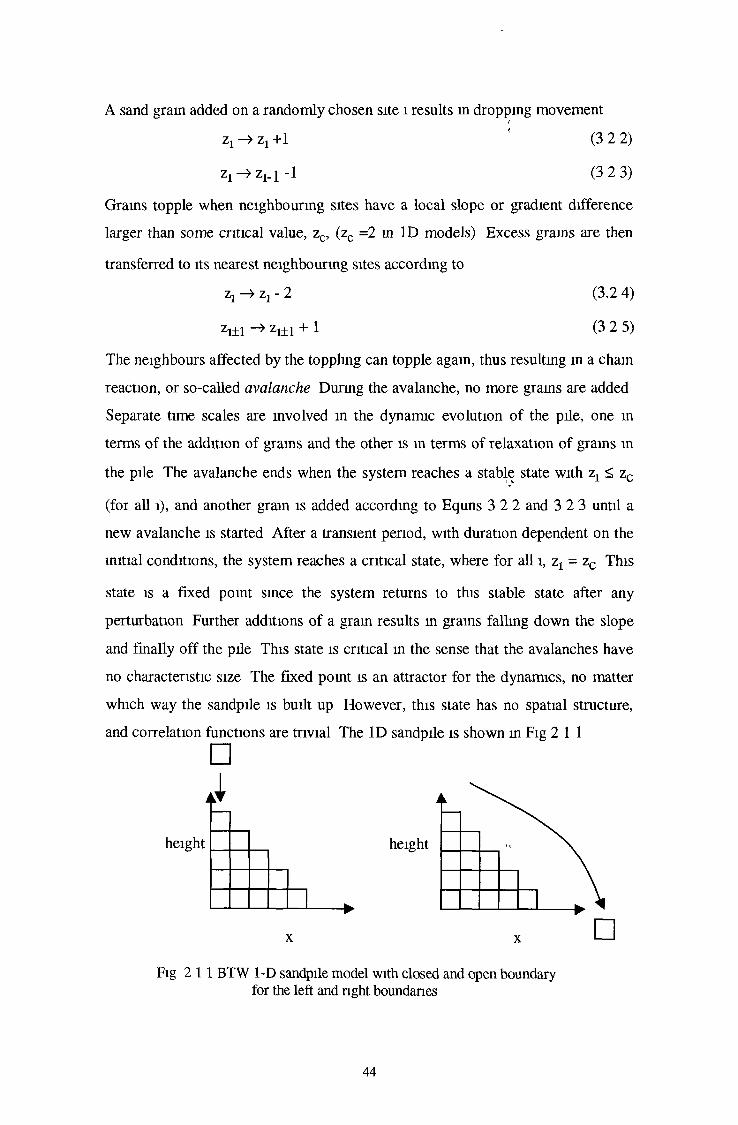
A sand grain added on a randomly chosen site 1 results in dropping movementt

z l —» z l +1 (3 2 2)z1 —> z t_i -1 (3 2 3)

Grams topple when neighbourmg sites have a local slope or gradient difference larger than some critical value, zc, (zc =2 in ID models) Excess grams are thentransferred to its nearest neighbourmg sites according to

Zj —> Zj - 2 (3.2 4)Zj+1 —» Zj+i + 1 (3 2 5)

The neighbours affected by the toppling can topple agam, thus resultmg in a cham reaction, or so-called avalanche During the avalanche, no more grams are added Separate time scales are mvolved m the dynamic evolution of the pile, one m terms of the addition of grams and the other is in terms of relaxation of grams in the pile The avalanche ends when the system reaches a stable state with z, < zc(for all i), and another gram is added accordmg to Equns 3 2 2 and 3 2 3 until anew avalanche is started After a transient period, with duration dependent on theinitial conditions, the system reaches a critical state, where for all i, z l = zc Thisstate is a fixed pomt smce the system returns to this stable state after any perturbation Further additions of a gram results in grams falling down the slope and finally off the pile This state is critical in the sense that the avalanches have no characteristic size The fixed pomt is an attractor for the dynamics, no matter which way the sandpile is built up However, this state has no spatial structure, and correlation functions are trivial The ID sandpile is shown in Fig 2 11□

height height

□Fig 2 11 BTW 1-D sandpile model with closed and open boundary

for the left and right boundaries

44

1

The situation is different for the two-dimensional model where parallel rules are applied The 2D sandpile model is typically considered for a square lattice, with each lattice site (i,j) characterised by an integer z ^ (where i,j = 1,2, L) The integer Z(, ^ can be taken to represent a dynamical variable such as height, slopeetc for a site (i,j) in a spatially extended system Sand is added one gram at a time to a randomly chosen site, thus increasing the dynamical variable by one unit, z ^—> z^ j) + 1 Whenever the dynamical variable exceeds a threshold value z ^ > zc,at a given site, then the whole column of sand is redistributed among the neighbours, leadmg to a series of topples which may give rise to an avalanche and which subside after a finite period of time The simple dynamical rules satisfy local conservation through

z0 , j ) ^ z( i j ) - 4 <3 2 6 )

z ( i± l j ± l ) z (i± l,j± l) +1 ( 3 2 7 )The pile eventually achieves a statistically steady state and any additional sand gram will fall off the open boundary This is a dissipative relaxation mechanism since it is accompanied by loss o f energy through the boundary Here we show a sequence of toppling events m a very small system for illustration, (Fig 2 12) The number m the squares represents the heights If a grain o f sand is added to a site with height 3, it causes that site to topple Eventually, as toppling diminishes, the system comes to rest There are nine sites toppling m the example shown, so the avalanche has size s=9 for this particular perturbation The total duration time, the number o f update steps, t=7 of the avalanche

'A

45

1 2 0 2 32 3 2 3 01 2 3 3 23 1 3 2 10 2 2 1 2

1 2 0 2 32 3 ,2 3 01 2 M i 3 23 1 3 2 10 2 2 1 2

1 2 0 2 32 3 3 3 01 3 0 iH 23 1 iH 2 10 2 2 1 2

1 2 0 2 32 3 3 4 01 3 2 0 33 2 0 10 2 3 1 2

1 2 0 3 32 3 0 11 3 2 2 33 2 1 0 20 2 3 2 2

1 2 1 3 32 ■ 0 1 11 3 3 2 33 2 1 0 20 2 3 2 2

1 3 1 3 33 0 1 1 11 3 2 33 2 1 0 20 2 3 2 2

1 3 1 3 33 1 1 1 12 0 ¡¡¡1 2 33 3 1 0 20 2 3 2 2

1 3 1 3 33 1 2 1 12 1 0 3 33 3 2 0 20 2 3 2 2

<

Fig 2 12 Illustration of topping avalanche in a small sandpile in a BTW 2-D model Within the avalanche of size 9, one site has toppled twice The black squares indicate the eight sites that toppled

For the 2D sandpile, the critical state for which all sites have exactly the critical slope is not stable any more due to small perturbations An avalanche would spread into two directions on the lattice with more than one gram falling off the pile, and it is not a fixed pomt as m ID However, after a transient period, the system through a self-organizing process reaches a stable critical state where, on average, the rate of flow mto the system equals the rate o f flow out o f the system across the boundary The stationary state then responds to the addition o f a sand gram with an avalanche This is o f unpredictable size, (number o f toppled sites), and duration, (number of iterations needed to reach the stable state), so that size and lifetime distributions vary over large scales Statistically, the probability distributions of the size s and lifetime t averaged over a large number of perturbations have been observed to follow power-laws

P(s) ~ s1’1 (3 2 8)P(t) ~ t b' (3 2 9)

where t and b' are defined to be the size and lifetime exponents respectively, with

46

no characteristic time and length scales If we define P(s, L) is the distribution function of avalanches s for a system of size L, then we have

P(s,L) = LpF(s/LY) (3 2 10)where p is a decay exponent, (3= y (i-1) (x defined by Equn(3 2 8)) y is a criticalindex which represents how the cutoff scales with system size and F is a scaling•?function When L—>oo, the avalanche size distribution becomes independent of the system size L, and when s/LY—>0, F approaches a power law and decays very quickly for s » LY, Tang (1988)

3.2.1.2 Catalogue ofSandpile ModelsMany sandpile automata models have been studied to date In the critical height model, the integer variable z represents the height of the sand column at the site (i,j), i e is dependent on zero derivatives o f the local sand height function being equal to zero The critical slope model is defined to depend on the first derivatives of the local sand height function, i e strictly is a local gradient rather than overall slope and the critical Laplacian Model is dependent on the second derivatives of the local sand height function, Manna (1991) Of the various sandpile models the height version in particular has been intensively studied because of its intuitive form and the simplicity o f its mathematical structure, Lubeck and Usadel (1996) However, the critical slope model even the local gradient version behaves in a way which is much closer to a real sandpile Formulation of the model is similar to Equn (3 2 6) but differs in that if the local slope in any direction exceeds the critical slope, then the sandpile topples Early studies, e g Manna (1990), Ruskin and McCarren (1994) failed to find evidence for simple power-law behaviour, so that scaling in the avalanche cluster and duration distribution function does not appear to be satisfied Here "scaling" means that distribution and correlation functions for all dimensionless quantities are constant in tune For additional work on the slope model see, e g Puhl (1992), Frette (1993) and references within For the critical Laplacian model, studies by Kadanoff et al (1991) have shown, through a scaling analysis, that the exponents are different from the critical height model, and the model thus belongs to a different "universality" class The key equation is

47

L(i,j) = 4h (y) - h(l+1 J} - h(lJ+1) -h(l. ld) -h(lJ_1} (3 2 11)where L (ij) is the local LaplacianZhang (1989) proposed a different stochastically driven continuous energy model He considered a real number E ^j) represented at each site (i,j) on a square latticeThe system is perturbed randomly by adding an amount to a randomly chose site, i e E (y ) — +8E If the value at any site exceeds the threshold value E(1?j) > Ec, the system relaxes according to

e is an exponent for energy dissipation Similar to the 2D BTW model, when e=0 25, the system is conservative and dissipation occurs only at the boundary, where the number of nearest neighbours is less than 4 Zhang has studied systems with Ec =1 and 8E chosen uniformly in the interval [0,0 5], and found that thesame universality class as that for the BTW model applies, (i e values of critical exponents are in agreement with those obtained for the 2D BTW model)Another continuously driven dynamical system was introduced by Olami et al(1992) (OFC) in terms o f earthquake modelling Though the dynamics of earthquakes are very complex, the event is driven by slow relative motion of tectonic plates, and the occurrence o f abrupt shocks is intermittent There are two time scales involved m the process, one is related to the stress accumulation, while the other is associated with the duration of the abrupt releases of stress

3.2.2 Current Studies on Sandpile and SOC3.2.2.1 Theoretical Results

" t5jjSandpiles with SOC have also been studied by several theoretical approaches Mean-field theory has been used to neglect the effects of the fluctuations so that local variables are replaced by statistically averaged values, Tang and Bak (1988), Christensen et al (1993) One fundamental question of the mean-field approach is that of the upper critical dimension, l e the spatial dimension above which mean- field results are valid In most SOC models, this dimension seems to be 4, Obukhov (1988), Diaz-Guilera (1994)

E(i± l,j± l) -^E(i± l,]± l) +eE(i,j)E (i,j) -> o

(3 2 12)(3 2 13)

48

1

TjlV

Theoretical work by Ding et al (1992) on alternative models with stochastic slide, however, has led to the conclusion that small and large sandpiles belong to different universality classes This also provides some explanation for the apparent discrepancy observed with former experimental work, Held et al (1990) Another approach has been to investigate sandpile models where the rules are more suitable for obtaining analytic results, e g Abelian sandpile model, Dhar(1989), Creutz (1994) The renormalization group method is widely used in critical phenomena where the lack of characteristic scales is demonstrated frequently, Pietronero et al (1994)There has been a lot o f interest in constructing differential equations to describe the scale invariance o f cellular automata models For example, anomalous diffusion equations with singularities have been considered for studying the deterministic dynamics o f the avalanches reached in the critical state, Carlson et al (1990), Chau and Cheng (1994), Kadanoff et al (1992) Additionally, nonlinear stochastic differential equations have been used by the dynamic renormalization group to analyse the earthquake models, Hwa and Kardar (1989), Grinstein et al(1990), Diaz-Guilera (1993)

3.2.2.2 Experimental ResultsReal sandpiles o f course present very complex behaviour so that they are difficult to explain fully in terms of simple interaction rules For example it has been found that the existence o f SOC in real sandpiles depends on how the pile is built Two distinct types of experiments have been performedJaeger et al (1989) used the method of rotating a semi-cylindrical drum partially filled with sand' at a low constant velocity In this experiment, the drop number (defined to be no of grams tumbling at one tune stepVTwas found to be approximately periodic in time Held et al (1990) considered the case of critical- mass fluctuations m an evolvmg sandpile, through an experimental study where the sandpile was built up to a steady state and then subsequently perturbed by the addition of a smgle gram at a time After each gram was added, the size of the resulting avalanche was recorded Repeated perturbations showed that avalanches were not predictable m terms either of their individual size (weight) or of their duration

49

Held and his co-authors discovered that sufficiently small sandpiles showed broad scale-invariant distributions for avalanche sizes For larger sandpiles, theavalanche distributions become sharply peaked, and the scale-invariance breaks

%down demonstrating finite-size scaling and the existence o f SOC Experiment shows that a single gram of sand can cause avalanches rangmg from the extremely small to the system’s finite limitHowever, the observed behaviour indicates that inertial effects play an important role, Dhar (1992), Prado and Olami (1992) Inertial effects lead to a nonlocal process, whereas m the numerical models, only the local geometry determines the dynamics The relationship between the drop number o f sand grams measured m experiments and the avalanche size measured in numerical models is unclear Moreover, the work of Rosendahl et al (1993) deals with gram-by-gram quiescent perturbation of real sandpiles of various sizes for which it appears that power law behaviour is valid for all system sizes Mehta and Barker (1994) have recently reviewed theoretical and experimental dynamics o f granular material, which deals with some of these questions t*An experiment to mvestigate the relaxation dynamics o f a sandpile was performed by Jaegeret et al (1989) In their work, sandpiles initially at a given angle of repose were vibrated with varying degrees o f mtensity, and the relaxation of the average slope o f the pile was monitored It was found that for large intensities of vibration, the slope of the pile decayed to zero such that its relaxation was proportional to the logarithm of the time, whereas for smaller intensities, the slope of the pile stayed finite and the relaxation appeared slower than logarithmic In a more recent experiment, Frette et al (1996) have observed the mternal dissipated energy m a slowly driven one-dimensional ID rice pile It was shown that the occurrence of SOC depends on details m the gram-level dissipation mechanism With spherical grams, a stretched-exponential distribution was observed, implying a characteristic scale, and is mconsistent with SOC However, with more elongated grams, the dynamics were dominated^by sliding grams These mduced higher friction, and a power-law distribution of avalanche sizes was found This provides the first experimental results o f SOC behaviour m slowly driven granular systems Theoretical models o f rice piles are related to a

50

variety of different physical systems which share the same universality class, Paczuski and Boettcher (1996)

3.2.2.3 Computer Simulation ResultsThe study o f sandpiles and related systems exhibiting SOC has to a great extent been based on simulations that use cellular automata models Several factors which affect the behaviour exhibited by sandpile models have already been discussed Unsurprisingly, these factors together with the sample size (no of events or trials in the simulation) under various dynamics all have a direct bearing on the nature and precision o f the results obtained, Manna (1990) (1991), Ruskin (1993)As a final point, it is worth noting that both theoretical and simulation studies to date confine themselves to grains of a uniform size, whereas in a real pile the gram size is irregular leadmg to a virtually continuous avalanche o f the finest grams when the sandpile approaches the critical pomtWe now consider some specific examples of sandpile automata that we have implemented under various conditions and automata rules These illustrate behaviour corresponding to a variety of applications Systems sizes range from L=256, where L is the linear dimension of pile, to L=1024 *\!3.3 Studies of Sandpile Models

3.3.1 Simple Sandpile Height Models and SOCWe have looked m what follows at two versions of sandpiles namely (i) the simple height model with toppling rules as described m Section 3 2 1, (n) the direct random model, where directed refers to ther fact that toppmg is m a preferred direction and sharmg is random (as m (i)) This also use the height dynamicsFor the direct sandpile height model, we have used the square lattice with steady height values o f a site equal to 0, 1, 2, 3 and critical height hc =4 (Here we useheight variable h mstead of z) Thus for hc >4 the site topples Simple feature s ofsimulation have been varied namely lattice size = L2 and No ' o f trials (samples)

VThe range of L was 32 to 1024 at which size storage was already a problem for

51

the larger number of trials, which range from 10000, to 50000 and 100000 These examples were implemented on both VAX and UNIX systems available in DCU The dynamics of the directed model (m) may be described similarly to those of the simple undirected model, Equns ( 3 2 7 - 3 2 8 ) with an integer variables h(lj) associated with each site Again these are discrete and diffusive but are now supplemented by the preferred direction condition so that if any site h(lj) > hc, it will topple only if the direction o f toppling is allowed The local height h(lj) is then decreased We have again built the sandpile on a square lattice where =2, so that the two neighbouring forward sites j± = j± [l± (-l)1]/2 are increased by 1

h0 j) h( i j ) ' hc(ij) (3 3 1)

h(i+l, j±) h(i+l,j±) +1 3 2)i e when i = odd,

h(i+1, j) -> h(i+1 j) + 1 (3 3 2a)h(i+l, j-l) h(i+lj-i) +1 (3 3 2b)

when l = even,h(i+l, j+1) -> h(i+l,j+l)+1 (3 3 2c)h(i+1, j) h(i+1 j) + 1 (3 3 2d)

Starting with random initial conditions, a particle is added at one randomly chosen site at a given row of the lattice If at that site the condition is,satisfied, then two particles slide to the two nearest neighbours at the next row,’where the toppling condition may be fulfilled again, leading to more topples and so on We follow an avalanche until the system regams its stability, and then the next particle is added at the randomly chosen site Sand grams are allowed to leave the system when the avalanche reaches the boundary

3.3.2 Results and ConclusionsThe form of the size and time distributions o f avalanches is shown in Figs 3 3 1- 3 3 2 for modest system size L=512, as an example Similar results are obtamed for different systems we discussed above These show clearly that a scaling region exists, corresponding to the linear part o f distribution of avalanche size, l e log D(s) vs log s We observe that as the lattice size mcreases, the linear part is

52

smoother and increases in length for larger No of trials, permitting more precise estimation of the exponent, Equns (3 2 8-3 2 9), before degenerating into chaotic or noisy behaviour for very large avalanche sizes The largest avalanches observable are directly related to the number of particles in the sandpile so that a small sized sandpile necessarily limits the observation of large avalanches Averaging over a large No of trials or samples is clearly desirable in order to improve the statistics and we note that both No of trials and lattice dimension L are modest in this work The behaviour of the lifetime distribution vs log t is similar to that shown for sizeWe illustrate for L=512 and 10000 trials in Figs 3 3 1-2 Our estimates of the exponents x and b' are given to be x=l 81, b'=0 45 Comparing these with those quoted by Bak et al (1989), X=2 0, b'=0 43, Manna (1990), x=8/7, the simple decay exponent b'=19/15, Ruskin (1993) x= 1 016 to 1 093, b'=0 423 to 0 457, and b'= 1 012 to 1 119 for a perturbation of size 1 for L variable, (perturbation also variable, Ruskin (1993)), it seems clear that we have good agreement with previous results with respect to the lifetime exponent However, our value for x is rather high, compared to more recent results, but agrees reasonably well with the initial theoretical sandpile models, Bak et al (1987), Dhar et al (1989) which made rather simplistic assumptions on the fimte-size effect This discrepancy may be due therefore to the size o f the system which we have studied, compared to previouslyMore recently, Lubeck and Usadel (1997) have considered the directed BTW 2D sandpile model in a large scale, up to system size o f L=4096 They also introduce a new method for statistically analysing the data to reduce the fimte-size effects and obtain results, x=2 293 and b =1 48, which are in agreement with the results obtained by renormalization group approach, Pietronero et al (1990)

53

Log s

Fig 3 3 1 Distribution of avalanches size with L=512 and No of trials =10000

0 0 5 1 1 5 2 2 5 3 3 5 4

Log tFig3 3 2 Distribution of avalanches lifetime t with L=512 and No of tnals=10000

*•

3.3.3 The Directed Sandpile Model with Holes: Introduction for a Preliminary NoteWe have also studied for a small system, the directed critical height model on a 2D square lattice m which a fraction o f sites p are considered as holes Thus the

54

system is additionally dissipative The sand grains may also leave the system through these holes during the dynamic evolution The distribution of defect sites or holes is random and can be considered as either annealed (increasing the system temperature, for example to reach an energetically more stable configuration in which the free energy is minimized) or quenched, (quickly reducing the temperature o f a system, for example to trap a state favourable only at high temperatures) For the sandpile system, annealed defects arise when the probability p that a defect may occur at each lattice site is fixed only for a single event The distribution of defects is generated randomly for each event, and is not memorised for the next event Quenched defects arise when a distribution of defect sites is generated for each concentration p and held fixed during all events For the directed height model with holes, Figs 3 3 3-4 illustrate size and duration distributions for a typical No of tnals= 10000, where the first 10 % of trials are left for the system to reach the steady state It has been shown, Dhar et al (1989), Tadic et al (1992) that the existence o f a preferred direction should lead to a new universality class, compared to the undirected model previously discussed It is evident that our results differ from those obtained in the first model, (Section 3 3 2) No clear linear region is obtamed, particularly in the size distribution andjthis supports the view that directed and undirected models do; not follow similar scaling laws In fact, the evidence for scaling is weak from our effort in the directed case, but this work considered small-sized simulations only (even compared to the undirected case) and consequently, the statistics are poor Tadic et al (1992) noted that power-law behaviour for size and time with exponents T=0 43 and b’=0 30 It is less clear, however, how hole concentration affects this behaviour Our very small systems consider L=128, with concentration of defects (holes) given by p=0 and p=0 05 and p=0 2 Results obtained for the low concentration are similar to these for p=0 (no holes), but the systematic deviations m the numeric values compared to the limiting law of form (Equns(3 3 4-5)) are due to the finite duration o f the simulation imposed by the holes, l e distributions are truncated Tadic et al (1992) argued that the self- organised critical state is lost in the presence of defects if the modified dynamic rules violate locally the height conservation %

55

As a preliminary look at dissipative systems, we considered the Tadic et al Model of introducing holes into the board It is unlikely that small sandpiles under such restrictions can show the same wide range o f fluctuations, since as noted for simple piles, (Section 3 2 2 2), large and small pile can behave very differently Our limited study thus indicates that a crossover from SOC to non-SOC for a

idefective system is reached rapidly for small system size, but provides little qualification of this or comment on Equn (3 2 10) An extended investigation, however, should include a wider range o f p valuesFor more complex defect cases, Tadic and Ramaswamy (1996) have studied in

'i*detal three models of driven sandpile type automata in the presence of quenched random defects These models are termed the random site, random bond and random slopemodels and when the dynamics are conservative, the concentration-dependent exponents are nonuniversal In the case o f nonconservative defects, the asymptotic state is subcritical

Ln s

Fig 3 3 3 Distribution of avalanches size s for directed sandpile model with L=128, and No of tnals= 10000

56

Ln t

Fig3 3 4 Distribution of avalanches lifetime t for the directed sandpile model with L=128, No of tnals=10000

3.4 Dissipative Sandpile Models

3.4.1 Nonconservative Sandpile ModelThe origmal sandpile CA models are noise driven models in that the sand grams are added to randomly chosen sites m a pile, and either the local dynamics are conserved (i e no energy loss durmg the toppling) or the local dynamical law is conserved The BTW relaxation rules conserve the dynamical,variable z except at the boundary Earlier studies have shown that conservative interaction rules are essential for obtammg SOC m the sandpile models, Manna et al (1990), and are also obeyed e g m the earthquake model, Hwa and Kardar (1989) Further investigation has shown that only those nonequilbnum systems with either a conservation law or a special contmuous symmetry, demonstrate scale-invariance Grinstem et al (1990) However, more work on deterministic models, e g of earthquakes, demonstrates the existence of SOC without a conserved quantity and is intriguing as it suggests a different mechanism for overall scale-invariant structures, Christensen and Olami (1993), Olami et al (1992), Janosi and Kertesz (1993) The nonconservative model also demonstrates SOC, m the sense that the probability for energy release durmg an earthquake is a power law However, the model is found to be nonuniversal in the sense that exponents change contmuously

as a function of the parameters of the models Interest has also been directed to systems with uniform driving of the dynamics, Grassberger (1994) The evidence supports the view that scale-invariance holds for deterministic models of earthquakes, forest fires, and sandpiles, Middleton and Tao (1995), but not for others, e g a stochastic height sandpile model on the Bethe Lattice, Markosava (1995) It seems clear that the intrinsic features of dissipative systems and the real origin of SOC merits further exploration in view of these findings We have, therefore, considered some further examples of dissipative systems in more details The dissipative sandpile models in what follows, exhibit no local conservation of energy with fixed perturbation Sand is still randomly added to a site, generally resulting in avalanches in which the redistribution of sand grams is accompanied by energy loss according to local dynamical rules Grams reachmg toppling conditions at the boundary will ultimately fall out of the system

3.4.2 Various Dissipative Models3.4.2 1 BTW and Zhang Dissipative ModelsTwo simple types o f dissipative models were initially proposed, one driven by random discrete BTW model and the other the contmuous-energy Zhang model under local nonconservative conditionsOf interest is whether the BTW model retams critical behaviour when mtroducmg nonconservative dynamics m the interior of the system. The simple way to consider this is to change rule Equn (3 2 6), for example, to

z(i,j)^z(i,j) '5 (3 4 1 >with Equn (3 2 7) remammg unchanged, This means one gram of sand is lost or dissipated for every topple In the stationary state, the average rate of dissipation equals the average rate of flow into the system. Thus, <s> = l/P Zc where PZc is theprobability o f adding a gram to a site with zc units, causmg an avalanche This probability approaches a constant value when L—>°o, which means <s> will achieve a finite value It is obvious that such a system cannot display SOC The avalanche size distribution decays exponentially with a characteristic avalanche size, regardless o f the system size, and avalanches seem to be localized

58

With £<0 25 is chosen in Equns(3 2 11-3 2 12), the dynamics of the Zhang modelt

are nonconservative When 8E is chosen in the range [0 1,1], the nonconservative relaxation rule again produces a characteristic avalanche size This model is also noncritical in the presence o f nonconservation, Diaz-Guilera (1994), Vespignani et al (1995)

3.4.2.2 CA and CML Dissipative ModelsIn a two-dimensional conservative sandpile CA model, all the space, time and state variables are integer (Equns (3 2 2-3 2 3)) However, for the dissipative height sandpile model, this may not be the case since the local dynamics lead to changed values of local energy Using both CA and coupled map lattice (CML) models, (Kaneko (1989)), for a nonconservation system with both discrete and continuous fixed dynamics respectively, a parameter a is introduced for the former which gives local energy loss during the toppling events, 0 < a <1, with

sa=0 equivalent to no loss Therefore, in a two-dimensional model, Equn (3 2 5)

<

will be modified to beh(i±lj±l) = h (i±l,j±l) + ( ! - a ) (3 4 2)

We choose the same value for a for all the neighbouring sites of (i,j), and allow the neighbouring sites to topple simultaneously This fixed discrete amount of energy loss accompanymg gram toppling, results m avalanches which occur slowly compared to those for the nondissipative model, l e the lifetimes are longer The higher the value of a , the more energy is lost during the evolution For the contmuously driven dissipative model, i e the so-called CML model, we choose contmuous state variables Fn(i) in the lattice which evolve under a nonlinear function map f(x) to describe determmistically the loss of the local energy durmg a topple In contrast to the dissipative CA model, the corresponding toppling rule m a two-dimensional CML model may be given by

Vh(i±l,j±l) = h(i±lj±l)+Fn(i±l,j±l) ’ (3 4 3)

where we define Fn+1(i)=f(Fn(i)), (F0(i)= l) Smce the local energy loss must beless than or equal to the whole local energy available, the corresponding values Fn(i) must satisfy 0 <Fn (i) < 1, and correspondingly 0 < f(x) <1

59

We have chosen to use two different function maps f(x) representing different dissipation patterns which are either parabolic (non-periodic) or periodic respectively, 1 e

here a is a constant, 0< a <1 and when a=0, f(x)=l, and Fn(i)= l, local conservationholds The toppling and avalanche procedures in the CML models are similar to those of CA models, but the subsequent toppling energy distribution is influenced by the current toppling energy loss The dynamics o f this CML model resemble in some sense the continuous stick-slip earthquake model which has been discussed in Christensen et al (1992)It is obvious that the dissipative pattern observed depends on the choice of function f(x) Our choice reflects, to some extent, extreme conditions satisfymg sand transport, (Fig 3 4 1) Clearly, functions which correspond to more complex local dynamics can also be chosen In what follows, we investigate whether local conservation is either a necessary and/or sufficient condition for a dissipative system to exhibit SOC in both CA and CML dissipative models for various values of a and different choices o f f(x) respectively ''

3.4.3 Results for CA and CML modelsBoundary conditions are taken to be open only here, consistent with those in the non-dissipative models Periodic boundary conditions are considered in detail elsewhere, Middleton and Tao (1995) The mam influence o f the open boundary is to lead to contmuous loss o f the sand to its neighbourmg sites

3.4.3.1 Dissipative sandpile, CA modelWe have implemented the discretely driven dissipative CA model, Equns (3 4 2), with values of a = 0 03, 0 3, 0 5, 0 8 respectively Distributions o f size, s, and lifetime, t, are shown m Figs 3 4 2-3 4 3 We observe that distributions are qualitatively similar for the different values o f a The increasing dissipation m the CA model causes a decrease m the quantity o f avalanches^ Multiple toppling events do not occur any more due to the mtroduction of dissipation, and the

f(x)=l-ax2f(x)=l-asm(x)

(3 4 4) (3 4 5)

60

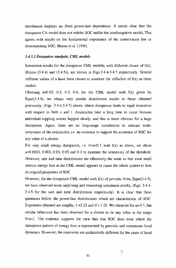
distribution displays no fixed power-law dependence It seems clear that the dissipative CA model does not exhibit SOC unlike the nondissipative model, This agrees with results on the fundamental importance o f the conservation law in demonstrating SOC, Manna et al (1990)

3.4.3.2 Dissipative sandpile; CML modelsSimulation results for the dissipative CML models, with different choice of f(x), (Equns (3 4 4) and (3 4 5)), are shown in Figs 3 4 4-3 4 7 respectively Several different values o f a have been chosen to examine the influence o f f(x) m these modelsChoosing a=0 03, 0 3, 0 5, 0 8, for the CML model with f(x) given by Equn(3 4 4), we obtain very similar distribution results to those obtained previously, (Figs 3 4 6-3 4 7) above, where dissipation leads to rapid truncation with respect to both s and t Avalanches take a long time to occur because individual toppling events happen slowly, and this is more obvious for a large dissipation Again, there are no long-range correlations to indicate scale- mvariance of the avalanches, i e no evidence to support the existence o f SOC for any value of a chosenFor very small energy dissipation, i e 0<a<0 1 with f(x) as above, we chose a=0 0003, 0 003, 0 03, 0 05 and 0 1 to examine the sensitivity o f the threshold However, size and time distributions are effectively the same so that even small interior energy loss in the CML model appears to cause the whole system to lose its original properties of SOCHowever, for the dissipative CML model with f(x) of periodic form, Equn(3 4 5), we have observed some surprising and interesting simulation results, (Figs 3 4 4- 3 4 5 for the size and time distributions respectively) It is clear that these quantities follow the power-law distributions which are characteristic of SOC Exponents obtained are roughly, x =2 25 and b '- 1 25 We illustrate for a= 0 1, but similar behaviour has been observed for a chosen to be any value in the range 0<a<l The evidence supports the view that that SOC does exist where the dissipative pattern of energy loss is represented by periodic and continuous local dynamics However, the exponents are qualitatively different for the cases of local

61

nonconservation and conservation modelsRecently, several authors have attempted explanations on the nature of SOC in these dissipative systems, Strocka et al (1995), Ah (1995) From our numerical simulation results, it appears that, for a dissipative model, SOC depends, at least in part, on the nature of the local dynamics rather than the conservation law

& s

”™ “1-a*sin(x)

--------1-------I-------I-------1-------1-------1-------1—

-------1-a*x*x

—i-------1-------(—0 10 20 30 40 50 60 70 80 90 100 110

X

Fig 3 4 1 The continuous variables F(x) of site x for two types of function f(x) (non-penodic and periodic respectively) representing local energy dissipation Both chaotic (non-penodic) and periodic behaviour are often seen m many physical systems

0 0 5 1 1 5 2

Fig 3 4 2 Distribution of avalanches with size s for the dissipative CA model

62

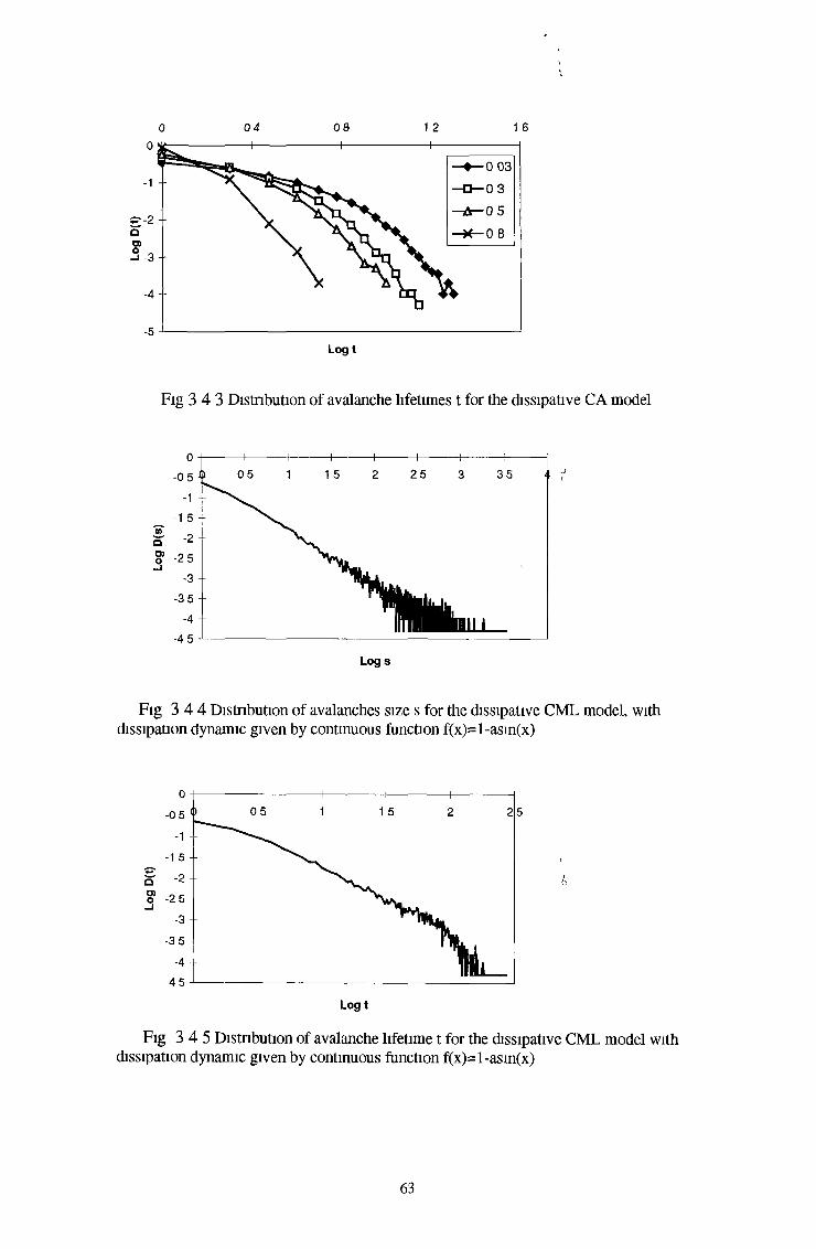
0 0 4 0 8 12 1 6

Fig 3 4 3 Distribution of avalanche lifetimes t for the dissipative CA model

Fig 3 4 4 Distribution of avalanches size s for the dissipative CML model, with dissipation dynamic given by continuous function f(x)=l-asin(x)

Fig 3 4 5 Distribution of avalanche lifetime t for the dissipative CML model with dissipation dynamic given by continuous function f(x)=l-asm(x)

63

0 0 5 1 15 2

Fig 3 4 6 Distribution of avalanche size s for the dissipative CML model with dissipation dynamic given by continuous function f(x)=l-ax2

0 0 4 0 8 1 2 1 6

Fig 3 4 7 Distribution of avalanche lifetime t for the dissipative CML model with dissipation dynamic given by continuous function f(x)=l-ax2

3.4.3.3 ConclusionWe have studied both discretely and continuously driven dissipative sandpile models, (CA and CML type respectively), under the height dynamic From the simulation results obtamed, we find no evidence for the existence o f SOC when dissipation is introduced mto the BTW, Zhang, and CA model Thus, a necessary and sufficient condition for SOC appears to be that the conservation law should hold, m agreement with fmdmgs of former authors However, SOC is apparently exhibited by some dissipative CML models, with results,from our limited investigation supportmg the view that local dynamics rather than local

64

conservation determine whether the phenomenon is observed This conclusion is in agreement with that for a deterministic dissipative model, Middleton and Tao(1995), but not with findings for a stochastically driven dissipative model on the Bethe lattice, Markosava (1995) Exponents for the avalanche distributions for s and t are quantitatively different for the local conservation and nonconsrevation models

3.5 SOC and Complex Systems

Most models for which we have discussed SOC are discrete in both space and time, they are cellular automata or some variants of CA More realistic models might involve infinities o f coupled differential equations, but for very many elements, it is unlikely that the discretization affects the asymptotic behaviour, w r t time and space in which we are interested Moreover, cellular automata seem particularly suited to systems with many metastable states, as in many of the complex systems that we consideredSandpile models clearly provide considerable and often contradictory insight into the phenomena of SOC Bak and Chen (1991) have concluded that the theory of SOC can be described in terms of many composite systems naturally evolving to a critical state, in which a minor event starts a chain reaction that can affect any number of elements in the system Although composite systems produce more minor events than catastrophes, cham reactions of all sizes are an integral part of the dynamics According to this theory, the mechanism that leads to minor events is the same one that leads to major events Furthermore, comp'osite systems never reach equilibrium but instead evolve from one metastable state to the next This theory clearly has attractions in terms of describing natural events, such as earthquakes The simplicity o f the models suggest that the phenomenon of SOC could be universal Certainly possibilities have been scrutinised by many researchers in various fields so far, e g statistical mechanics, condensed matter physics, geophysics, biology, and economy An interesting aspect is that the dynamics of SOC systems are intermittent, with avalanches of activity separating periods of relative quiescenceAnother important point is that avalanches are predictably displayed in long-term patterns, although it is impossible to predetermine when a system will reach

65

instability and how much adjustment is required to regain stability except on a short-term basis, Kagan and Knopoff (1987) Overall avalanches observed display a log-linear relationship for a real system, in agreement with that observed in earthquakes by Gutenberg and Richter (1956) These authors found a straight line with a slope (critical exponent) between -1 25 and -1 50 from earthquake model, depending on the fault under studyThe presence of defects in 2D directed sandpile automata leads to some interesting effects For the case of random defects, some concentration-dependent scaling exponents have been obtained, It appears that varying the concentration of defects is a mechanism for continuously tuning the local rules o f relaxation, which may finally lead to a phase transition between metastable states with different properties >In a slowly driven or evolving system, the physical time between lattice updates is very short when avalanches are propagating and very long when the system is being perturbed In the Zhang model, the transfer o f energy depends on the energy of the lattice, whereas it is a fixed quantity for the BTW models When introducing nonconservative relaxation rules into the stochastically driven BTW and Zhang models, the distribution of avalanche sizes decays exponentially with a characteristic avalanche size The systems are subcritical However, the occurrence o f criticality in some nonconservative models, e g continuous determimstically driven OFC model and CML models, is very intriguing since it suggests a different mechanism for the generation of the scale invariance (OFC model is an earthquake model, see Olami et al (1992)) Since moreover, the majority o f natural phenomena are nonconservative, the SOC behavior of nonconservative systems is probably more important to understand than the corresponding behavior of conservative systems

3.6 In Summary

In this chapter, we consider the problems involved in simulation methods applied to physical and related systems with few constraints Examples o f cellular automata modelled "sandpiles" and their applicability to real world systems have been described and the phenomenon o f SOC discussed. Recent theoretical

66

developments axe presented and assessed in terms of findings from experimental investigations Results of our implementations o f those models for both conservative and nonconservative systems are also given

67

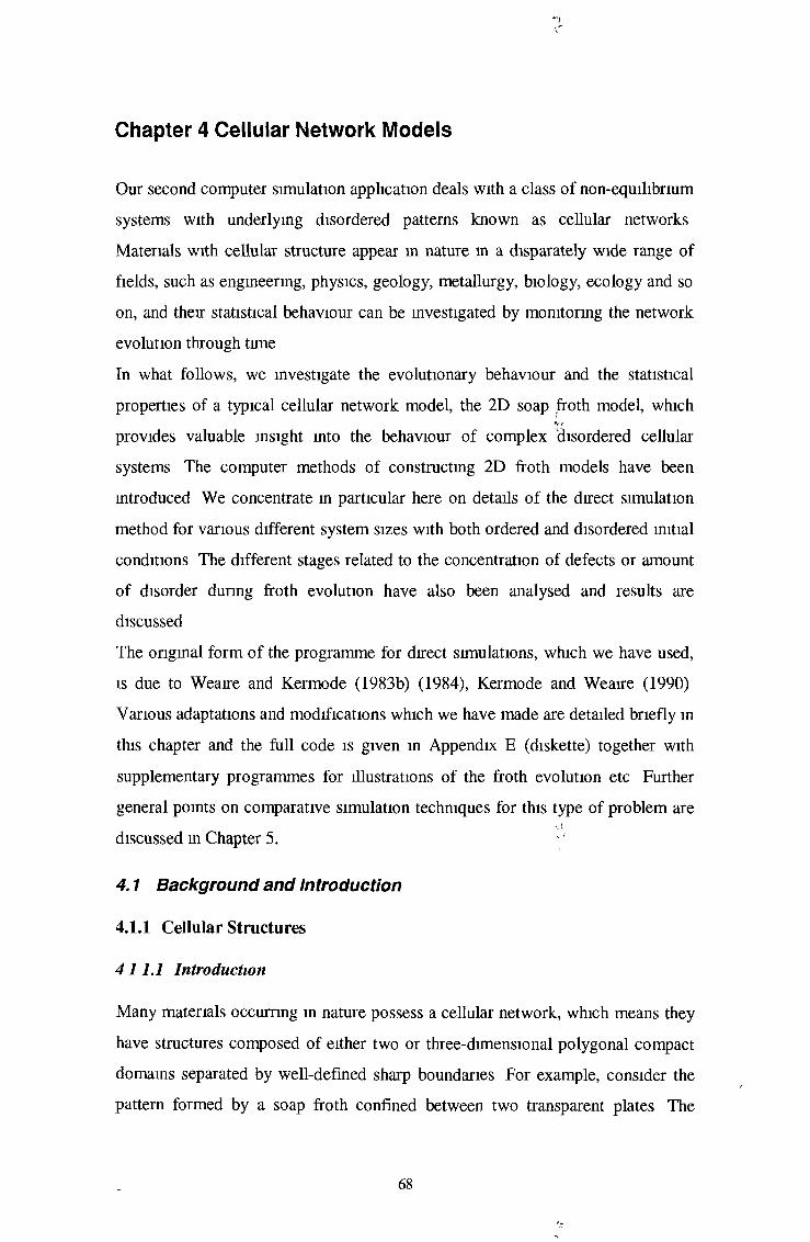
Chapter 4 Cellular Network Models

Our second computer simulation application deals with a class o f non-equilibrium systems with underlying disordered patterns known as cellular networks Materials with cellular structure appear in nature in a disparately wide range of fields, such as engineering, physics, geology, metallurgy, biology, ecology and so on, and their statistical behaviour can be investigated by monitoring the network evolution through timeIn what follows, we investigate the evolutionary behaviour and the statistical properties of a typical cellular network model, the 2D soap froth model, which provides valuable insight into the behaviour o f complex disordered cellular systems The computer methods of constructing 2D froth models have been introduced We concentrate in particular here on details o f the direct simulation method for various different system sizes with both ordered and disordered initial conditions The different stages related to the concentration of defects or amount of disorder during froth evolution have also been analysed and results are discussedThe original form o f the programme for direct simulations, which we have used, is due to Weaire and Kermode (1983b) (1984), Kermode and Weaire (1990) Various adaptations and modifications which we have made are detailed briefly in this chapter and the full code is given in Appendix E (diskette) together with supplementary programmes for illustrations of the froth evolution etc Further general points on comparative simulation techniques for this type o f problem are discussed in Chapter 5.

4.1 Background and Introduction

4.1.1 Cellular Structures411.1 IntroductionMany materials occurring in nature possess a cellular network, which means they have structures composed of either two or three-dimensional polygonal compact domains separated by well-defined sharp boundaries For example, consider the pattern formed by a soap froth confined between two transparent plates The

68

geometric structure o f this system consists of a tiling of the plane by domains or cells o f nearly polygonal shape In the three-dimensional case, the domains assume polyhedral-like shapes which are almost homogeneous and are separated by thin boundaries One of the oldest such patterns can be found in the Giant’s Causeway in North Ireland, Bulkley (1693) Samuel Foley (1694) first calculated the distribution function for a two dimensional network of grams A particular class of cellular structures, (which evolve either m time or as some external parameter is changed and for which an energy is associated with the boundaries), has become a subject of much mterest over recent decades Models of such patterns can be found in a wide range o f fields, e g soap froths, foams, magnetic bubbles m garnets, polycrystalline metals, alloys, and branches of physics such as hydrodynamics, Glazier and Weaire (1992)The applications of cellular network models have covered a wide range of areas For mstance, foams are beautiful examples of heterogeneous materials, with properties closely related to their structural characteristics The structures of foams are varied liquid foams, such as those made of the soap bubbles familiar to all, solid foams such as m cellular materials and so on The use o f foams ranges from transport o f granular media m pipes to fire suppression and explosion attenuation Thus the geometry of soap bubble arrangements m confined environments is an emergmg research subject, where several mtrigumg phase transitions have been recently observed, such as those with bamboo-like or spiral structures The problem of foam stability is more specific to liquid foams, however, and is connected with the important issue o f emulsion stability, Exerowa et al (1992), Aveyard (1995) We concentrate here on the studies of dry froth m which the liquid fraction is ignored, (1 e no Plateau borders), m order to demonstrate a direct approach to computer simulation of such systems Computational implications for extendmg these simulations to wet froths are briefly noted m final chapterWeaire and Rivier (1984) first mtroduced the type of cellular network problem described above, and this has motivated further developments on many aspects of cellular systems A more recent review, Stavans (1993), has put emphasis on the scalmg exponents characterising the time dependence o f the average scale of cellular structures m evolution Some specialised reviews also deal with important aspects o f particular systems, e g the geometric properties of biological tissues,

69

Dormer (1988), and the chemical application of solid foams and liquid foams, Goldfarb et al (1988)In contrast to the cellular system models, discussed in last chapter, any small perturbation in cellular network models will have an influence on all network elements, 1 e local adjustment will be related not only to nearest-neighbours, but also to second nearest-neighbours

4.1.1.2 HistoryThe soap froth as an ideal model o f a cellular network has attracted considerable attention in that it provides valuable insight into the behaviour o f several complex disordered systems Many efforts have been made to connect the soap froth model to other models in biology, metallurgy, ecology and so on As long ago as (1925) (1928) (1931), Lewis studied froth and living cells in an experiment on cucumber He recorded ordered and disordered patterns and gave an empirical relation between the number of sides of a cell and its area Some years later, Thompson (1942) noted the analogy between froth bubbles and cells o f biological organisms In particular, he quoted the similarity between grain growth in molluscan shells and a model of a crystal growing in albumin Bragg and Nye (1947) first proposed that froth could be used to model gram growth m metals, but had not deduced that the individual bubbles may be considered similar to atoms in whole crystal grams Later, Smith (1952) (1954) discovered that the soap froth represented the closest

jiapproach m an experimental system to ideal gram growth in a metal From this observation, his analysis shown that each separately oriented gram was analogous to one bubble m the froth and that gram boundaries m a metal corresponded to soap films Population biologists have further considered the influence o f cellular patterns during evolution For example, ecologists deal not only with behaviour withm a single habitat but also with the mteraction between an ensemble o f them, as for instance in the territorial competition m fish and other species, Hasegawa and Tanemura (1976)

70

4.1.2 Applications: Soap Froth Model4.1 2.1 Basic Geometrical Relations and Topological Process

iThe dynamics in a cellular structure are driven by surface tension or surface energy forces The structure consists of a network of boundaries on a surface, which has the property that three boundaries meet at every mtersection or vertex for the two-dimensional case A two-dimensional cellular structure embedded on the Euclidean plane consists o f a tiling of non-intersectmg polygonal cells or faces, whose boundaries are formed by curved edges impinging on vertex points According to Euler’s theorem, in general form, the relationship between the number of faces F, edges E and vertices V of a polygonal domain can be expressed as

F - E +V= % (4 1 1 )where % is the Euler characteristic Then % =0 for a network on the surface o f a torus (or for a planar network subject to periodic boundary conditions) and %=2 for a network on the surface of sphere in which case the network is topologically equivalent to a convex polyhedron, (the original application o f the result) Then %=1 corresponds to a finite network on the infinite plane The 'fundamental nature

i

of Euler’s theorem for topology comes about because the invariant it represents specifies the topological type o f the surface on which the network is drawn The network is built o f polygonal domains whose boundaries join at vertices with coordination number equal to three in cellular structures Applymg this theorem to large networks, we have that the average number of sides per polygonal domain is equal to sixDuring the evolution of a cellular structure, there are changes in the local connectivity o f the edge network These changes can be broken down into elementary processes or transformations, which obey the topological constraints There are two basic types o f topological rearrangements which have been observed in soap froths, foams and metallurgical gram aggregates, namely, T1 and T2 processes, which preserve topological properties by effecting changes m the number of sides of the cells mvolved m the transformation The T1 and T2 processes are shown m Figure 4 1 1 (a), (b) and (c), where for the T1 case two cells lose one side each and two others gam one For the T2 process, a cell with more than three sides can vanish through a series of T1 processes, to make it

71

three-sided, for example, in (b), the three-sided cell disappears with each neighbour losing a side, in (c), the four-sided cell disappears with the number of sides of two neighbours remaining constant while that o f the other two decreases by one Similarly, for the five-sided cell, the number o f sides of two neighbours is left constant, two other neighbours lose one side each and the fifth neighbour gams a side And so on for six, seven and higher order cells

(b)

(c )

Figure 4 11 Elementary Topological Processes(a) Side Swapping or T1 process(b) Disappearance of a three-sided bubble or T2(3) process(c) Disappearance of a four-sided bubble or T2(4) process

It is noted that four-sided cells have two possible decay configurations m contrast to three -sided cells whose decay state is unique Smce the classic work of Smith (1952) on soap froth, it has been conventional wisdom to think that T2 processes of four-cells do not occur Accordmg to Smith, the vanishmg of four sided bubbles is mediated by T1 processes m which bubbles become three sided first and then decay directly by shrinking This claim has not been vmdicated, however, by experiments on froth or m other cellular structures, where direct vanishmg o f four- and five-sided cells is observed, Glazier et al (1987) Theoretical support for the experimental results has been provided by Fradkov et

72

al (1993) The authors pointed out that the decay configuration which a fourfold or fivefold vertex will adopt, from all those possible in a particular situation, is determined by system-dependent characteristics such as the physical size o f the boundaries with respect to the system thickness They argue that this may endow the evolution with a stochastic character

4.1.2 2 Von Neumann’s Law and Scaling StateIn cellular network systems, a balance o f forces imposes restrictions on the angles between boundaries at each vertex Generally speaking, in a real case, it proves impossible to satisfy these restrictions unless boundaries are curved Evolution is driven by mechanisms that relax this curvature and thus minimise boundary length The simple and elegant theoretical basic to describe the dynamics of curvature-driven cellular network structure is due to Von Neumann (1952) and was supported by the original soap froth experiments o f Smith (1952)Von Neumann showed that the rate o f change of area with time of an individual cell and its number o f sides n are related by the expression

dA/dt = k(n-6) (4 1 2)Here A is the area of an n-sided cell and k a constant which depends both on the solubility o f the gas which diffuses through the soap film and the thickness of the latter However, a possible variant of Von Neumann’s law was recently proposed by de Icaza-Herrera and Castano (1995), which took into account the effect of cell's area as well, given as

dA/dt = kA(n-6) (4 1 3)We compare these equations of froth coarsening from different initial>configurations in due course tClearly, Equn (4 1 2) means that only a cell with less than six sides shrinks, while that with more than six sides grows A cell with six sides neither grows nor shrinks, although it may change its shape, as diffusion proceeds, until such time asit is involved in a topological change, when it no longer has six sides This isshown in Fig 4 1 2 and is particularly important in relation to transient behaviour since we can regard diffusion as occurring during the topological transformation processes according to equation (4 1 2)

73

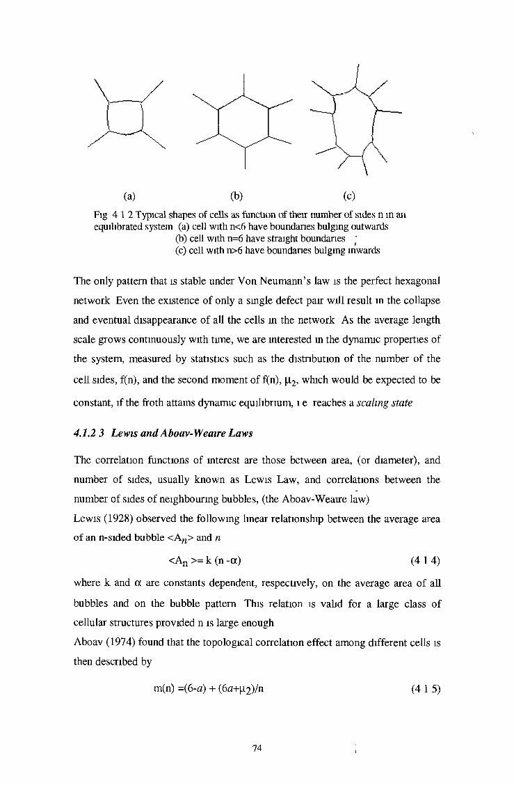
(a) (b) (c)Fig 4 1 2 Typical shapes of cells as function of their number of sides n in an equilibrated system (a) cell with n<6 have boundaries bulging outwards

(b) cell with n=6 have straight boundaries '(c) cell with n>6 have boundaries bulging inwards

The only pattern that is stable under Von Neumann’s law is the perfect hexagonal network Even the existence of only a smgle defect pair will result m the collapse and eventual disappearance o f all the cells m the network As the average length scale grows contmuously with tune, we are mterested m the dynamic properties of the system, measured by statistics such as the distribution of the number of the cell sides, f(n), and the second moment o f f(n), \i2, which would be expected to be constant, if the froth attams dynamic equilibrium, 1 e reaches a scaling state

4.1.2 3 Lewis and Aboav-Weaire LawsThe correlation functions o f mterest are those between area, (or diameter), and number of sides, usually known as Lewis Law, and correlations between the number of sides o f neighbourmg bubbles, (the Aboav-Weaire law)Lewis (1928) observed the foliowmg linear relationship between the average area of an n-sided bubble <An> and n

where k and a are constants dependent, respectively, on the average area of all bubbles and on the bubble pattern This relation is valid for a large class of cellular structures provided n is large enoughAboav (1974) found that the topological correlation effect among different cells is then described by

<An >= k (n -a) (4 14)

m(n) =(6-a) + (6a+|_i2)/n (4 15)

74

where a is a constant (a- 1 2), and m(n) is the average number o f sides o f the neighbours of an n-sided bubble This is known as Aboav’s Law and for the special case of a = l, is usually called the Aboav-Weaire law

4.1.2.4 Simple Soap Froth M odel

The soap froth is the simplest and most familiar structure which has the characteristic o f surface-energy-mimmisation, 1 e each cell is of some constant predetermined area (in two-dimensions) and the system is in equilibrium when the total length of all cell edges is a minimum with respect to any small distortion It represents the closest analogy to an experimental system with ideal growth A soap froth has all boundaries equivalent, with its evolution driven by a transfer of gas between neighbourmg bubbles and governed by Von Neumann’s law This constraint can be satisfied only if the boundaries are curved We focus on an ideal

tdry froth, where the balance of forces gives all internal angles o f the network equal to 120° and the mean number of sides <n> =6 Evolution is through T1 processes (neighbour switching) and T2 processes (cell vanishing), (Fig 4 11) From Equn (4 12), we obtain the average area o f a bubble <A> to be proportionalto the time, t, i e asymptotic linear scaling of the froth, <A> ~ t a Also, it can be predicted that in a scaling state, the average length scale, <d>, has the form <d> ~ tP, where (3 is the growth exponent The pattern of the froth is also characterised by a single length scale, the mean cell radius <r>, (<d>= 2<r>) The average size of the cell is a function of tune, m the sense that it gets smaller or larger as time goes onFurther a random structure can be characterised in terms of the distribution functions o f its properties, namely the probability that a given bubble has a given area relative to the mean area, <A>, o f the pattern and the topological distribution

lj'function f(n), the probability that a bubble in the pattern has n sides Thus, moments are given by

(416)

By definition from equation (4 1 6), (j,0 =0, |i, =0 The dispersion and skewness of the distribution is measured as usual by the second and third moments In the evolution of a froth, the value o f the second moment |H2 is a fundamental quantity

75

4.2 Current Studies of Froths

4.2.1 Experimental Studies and ResultsThe first experiments on coarsening of soap froth were carried out by Smith

V(1952), based on some photographs taken during the evolution’ of a froth, initially non-uniform which was observed to evolve from a few thousand tiny bubbles to a few hundreds While Smith found that soap froth mimics grain growth in metals, the former does not include the complexities of gram boundaries with orientation- dependent energies Smith’s analysis suggested that long-term asymptotic behaviour was just a change o f scale, with no change o f the side distribution He also found that dynamic scalmg properties can be characterised after initial transience by system statistics such as the second moment, |i2 =1 5 and the average area o f a bubble <A> dependent on an exponent, as mdicated previously, with a = 1 There was a tendency towards a fixed, time-independent distribution of number o f sides and relative sides He concluded that only three-sided bubbles could disappear directly, however, as noted earlier, whereas four-and five-sided bubbles could not, but evolve through T1 processes to become three-sided first, then vanish directly via a T2 processSmith’s conclusions were challenged by an analysis published by Aboav (1980), based on a different set of photographs o f Smith, usmg an alternative experimental method, where the initial bubbles were formed with roughly uniform size Evolution was agam followed from thousands of cells to hundreds of cells From the statistical data, Aboav found that no stable limiting distribution of sizes existed and the second moment |u2 ~ <d>, (roughly from 0 64-2 86), increased with average linear mtercept <d>, where <d> ~ <A>1/2, i e a=2 Much later, Glazier et al (1987) carried out a set o f experiments and found that T2 processes could mclude direct disappearance of four- and five-sided bubbles without any prior side-sheddmg Several types o f initial condition both ordered and disorder were considered In the ordered case, large ordered domains of six- sided bubbles are separated by dislocations formed by pairs o f five- and sevensided bubbles As t mcreases, five-sided bubbles shrink while seven-sided ones grow As the five-sided bubbles disappear, they affect the number o f sides o f the neighbouring hexagonal bubble and the spatial extent of the ordered regions

76

steadily decrease Once all the ordered domains disappear, evolution proceeds with disordered configurations A relaxation region is thus found followed by power-law behaviour Glazier et al (1987) found that, irrespective o f the nature ofthe initial conditions, froth evolution behaved asymptotically as <A>~ta with a=0 59±0 11 The difference with the expected value a = l was traced later, to the fact that the experiments were performed with a fixed amount o f fluid Stavans and Glazier (1989) studied the long-term scaling regime in terms of the■idistribution f(n) and its dispersion in both ordered and disordered froths Within experimental error, f(n) remains unchanged during the evolution after transient states have died out A more precise measurements of f(n) is also given, comparing results from a number of systems, they observed that f(5) is higher than f(6) They also provided evidence for the validity o f the Aboav-Weaire law, with the second moment ]i2 =1 4, and obtained excellent agreement with the measured dependence o f m(n) on n.

4.2.2 Theoretical ResultsSeveral theoretical analytical methods have been used to describe the evolution of cellular networks from various aspects(I) Mean-Field TheoryFlyvbjerg and Jeppesen (1991) derived a time-independent equation for the normalised distribution by introducing a generating function and solving analytically the partial differential equation obtained Furthermore, Flyvbjerg (1992) has obtained a master equation, which is very similar to that o f Fradkov et al (1988), but without assuming a maximum entropy distribution of the area A numerical solution was obtained for the distribution of the number of sides without any free parametersStavans et al (1991) pursued from the onset a two-track approach separating the calculation o f areas from that of purely topological properties They wrote dynamical equations for the variables without including T1 processes as a first step The form of the equations neglected the appearance o f two-sided cells They found a line o f fixed points instead of a unique fixed point as one would naively expect Results here support the asymptotic tune-independent behaviour of froth Recently Segel et al (1993) extended the approach o f Stavans et al to the

77

i

calculation o f area-related properties Their results are in agreement with experiment for all values of n and Lewis’s law is valid for large values o f n(II) Maximum Entropy MethodEeenakker (1986) used a hybrid approach to describe the evolution of a froth He derived a dynamic equation for the area distribution function He argued that scaling behaviour is not exhibited in the solution Instead, some cyclic behaviour is obtamed, whereas disordered configurations collapse into ordered ones, consisting mostly o f six-sided cells Then evolve to disordered again No such behaviour has been seen in any experiment so farDe Almeida and Iglesias (1988) have studied maximum entropy to calculate the topological functions Their predictions for side distribution f(n) is in agreement with those obtamed from froth experiments, corresponding to the second moment, \i2 =1 5 However, the area distributions do not match experimental data for anyvalue considered(III) Topological ModelLevitan (1994) first proposed a topological model to implement the rearrangement of the froth by random T2 processes He considered the froth m terms of the areas of the bubbles and constructed an approximate topological realisation of the froth structure by labelling sites of the bubble lattice to create an adjacency matrix of nearest-neighbour connectivity His model was used to solve von Neumann’s equations on a geometrically realistic network of bubbles up to the pomt when the first bubble disappears Since a T2 process is selected randomly, the neighbouring bubbles change their topological classes corresponding to the adjacency matrix changes This model has also been unsuccessfully applied to the analysis o f a smgle defect m a hexagonal network, Section 4 3 2 Recently, Levitan and Domany (1995) (1996) have proposed subsequent, revised versions o f this topological model to correct the former results Some extra assumptions have been taken to apply to the ongmal model One such, takes mto account the effects of the areas o f the topological classes o f the neighbouring bubbles on the results of a T2 process Lengths o f the sides of 4-sided and 5-sided bubbles are calculated to obtam specified rectangles and pentagons of bubbles The obvious advantage of these topological models is that they can deal with the macroscopic evolution of a froth with a very large system size They have also been used to observe the

78

4<r

behaviour of the remaining bubbles, (so-called survivors) in some detail, Levitan and Domany (1997) A system size of over 40,000 bubbles has been studied so far However, results and conclusions obtamed by those topological models seem in poor agreement with those by experiment and simulation methods Some details are given in the following section(IV) Logistic Map TheoryRivier (1985) first suggested describing the froth network using a logistic map, which means a space-filling pattern consisting of a central cell surrounded by concentric layers of cells For detailed definitions and proofs, see Rivier and Aste(1996), Aste et al (1996) Applying this dynamic map to the froth structures, Aste and Rivier (1997) studied the topological properties o f physical froths, which are cellular networks with homogeneous shape and sizes They have found that in 2D, the logistic map has one parameter, given as a function of the average topological properties o f the cells in the layers The curvature of the space tiled by the froth

•y*1can also be obtamed from their calculationsFrom this shell structure map, a clear illustration is also provided of diversity between cellular networks and simple cellular systems While both consist of simple cells, the difference m the evolution laws is mtrmsic Connectivity relations between cells m the network are widespread and pervasive as opposed to local Any cell can be influenced by the disturbance m the network even it is far away from the central cell and the network adjustment take place mstantly Whereas only the nearest neighbour sites of the cell can be affected m a simple cellular system m the first step, i e the connectivity is local However, cellular automata rules govern transitions between these simple elements As we described earlier m Section 2 4 the local adjustment occurs simultaneously, while the whole system is adjusted m subsequent time steps

4.2.3 Computer Simulation Algorithms and Early Results i

Investigating a 2-D froth gives us the opportunity to observe the details of the structure smce it is easier to visualise and model than a 3-D one Generally speaking, four methods to date have been used to simulate froths These are (i) direct simulation (n) the Monte Carlo method (m) the vertex model (iv) the Potts

79

model (variant of MC) We discuss these alternative approaches briefly in whatfollows, concentrating on (1) for specific studies described later in the Chapter

i,4.2.3.1 Direct SimulationWeaire and Kermode (1983b) (1984), Kermode and Weaire(1990) proposed a 2D-FROTH program to investigate the equilibrium properties This program creates a finite sample o f the froth network model with periodic boundary conditions and equilibrates it by an iterative procedure The pattern reaches equilibrium by a repeated cycle of local adjustments The soap froth is a strictly chaotic system, so the detailed evolution of the pattern may depend on the sequence in which adjustments are made The program distinguishes between topological and diffusive adjustmentsMost studies so far assume that the cellular network is incompressible, and in the case o f a froth, attempts to compress it simply minimise the surface energy of the soap film at all tunes The radius of curvature of each side is

r= c(P ,-P 2)-' (4 2 1)Iwhere Pj and P2 are the pressures in the two adjacent cells and c is a constant

related to the surface tension T byc=2T (4 2 2)

These conditions are satisfied for each cell areaAssuming that the rate of diffusion R of gas across each side is proportional to the length / of that side and to the pressure difference across it

R=kl(P1 -P2) (4 2 3)where k is a constant According to Equn (4 1 2), only the cells whose number of sides n^6 contribute to froth evolution The cells with fewer than six sides will shrink and those with more than six sides will growThe local variables chosen to relax at each step, are the position o f a vertex and the pressures o f the three surrounding cells Although two arcs with the same curvature can be drawn to connect two vertices, it is assumed that it is always the smaller arc that occurs in the network, (also supported by the experimental evidence)Equations expressing the dependence o f the vertex angles and their neighbouring cells areas are given by

80

d A l d A l d A l d A \ dA \ "Apl" 'AA1~d p i dp2 dp3 dx dy dA 2 dA2 dA 2 dA2 dA2 A p2 A A 2d p i dp2 dp3 dx dy dA3 dA3 dA3 dA3 dA3 A p3 A A3d p i dp2 dp3 dx dy d(j) 1 dtpl d(j)l d(j) 1 d(j)l Ax Aipld p i d p 2 d p 3 dx dy dtp2 d(j) 2 d(j)2 d<p2 d(j)2 Ay A</>2d p i dp2 dp3 dx dy

nwhere p i, p2, p3 are pressures and x,y are vertex co-orduiates

V

so Equns (4 2 4) as a function of the five variables are approximated by a linear form, and numerical differentiation is used to determine the coefficients The angles and areas change as the froth equilibrates (i e angles optimum at 120°), and area adjustments involve vertices o f other cells alsoSince the topological changes (T1 and T2) are the essential mechanism of froth evolution, direct simulation implements these topological rearrangements in a direct way This means that after each local relaxation o f a vertex, the first step is to test the possibility o f a T1 process then specify the adjustment by solving the equations If the proposed displacement is D, and R, are vectors linking the vertex

81

in equation to its nearest-neighbours, then a T1 process takes place if the following is satisfied

D • R, >R, • R, (4 2 5)The T2 process only occurs in two cases Firstly, and most frequently, is in the diffusion procedure where changes of area are calculated A T2 process will take place if the target area is zero or negative Secondly, wherever it is convenient for a cell to disappear, then the target area is designed to have a small positive value The existence o f very small cells can cause some problems in the program, so any cell with area less than 0 1% of unit area, is forced to disappear (convergence)As noted above, the diffusion process involves a transfer gas across boundary The net rate of diffusion for a cell is given by Equn (4 1 2) and governs the cell area The total area remains the same and the average number of cell sides is six, see Section (4 1 2 1)

The 2D FROTH program structure is as followsPROGRAM FROTH

CALL SETUP // Create Voronoi networkCALL INPUT // Input parameters CALL STAT //Initialise

//Start evolution loop //DO 10 1=1,IJSTEP // Increment step number

ISTEP=ISTEP+1 CALL DIFFUS //Diffuse networkCALL EQUIL //Equilibrates the networkCALL STAT //Performs statistical calculations

10 CONTINUECALL OUTPUT CALL STATCALL EXITFR //Exit the programEND

Early results showed that for small system size equal to 100 cells, the simulated froth did not reach a scaling state, and \x2 increased (roughly) in a linear fashion with time For several samples of 500 cells, with differing initial structures, Weaire and Lei (1990) obtained the asymptotic value of |ll2 =1 42±0 05 Simulations

82

starting from ordered configurations showed an early increase of |12 followed by adecrease and eventual achievement of a steady state value Initial configurations characterised by different degrees o f disorder were allowed to evolve and in all cases scaling was achieved Herdtle and Aref (1991) using a similar method to Weaire and Kermode, however, obtained |i2 =1 2 for a system of size 1024 cellsThe difference hes mainly in the way the structure is relaxed towards equkbrium, which Kermode and Weaire (1990) specified as a sequence of'local adjustments of pressures and vertices, whereas Aref and Herdtle considered all these variables to be adjusted simultaneously in each iteration

4.2.3.2 Monte Carlo MethodThe Monte Carlo method depends on representing the solution of a problem as a parameter of a hypothetical population, and using a random sequence of numbers to construct a sample o f the population, from which statistical estimates of the parameter can be obtained Wejchert et al (1986) discussed the Monte Carlo simulation of the evolution of a two-dimensional soap froth, based on discretization o f the problem These authors used a triangular lattice which has six nearest neighbours in two-dimensional space ( le has a hexagonal dual) Two neighbouring lattice points with different assigned integers are automatically separated by a cell boundary A clustered group of lattice points labelled with an integer k, represents a particular bubble kThis method incorporates explicitly the rapid equilibration o f boundaries present in soap froths All cells involved are of uniform same size and shape This equilibration was also performed under the constraint o f constant bubble area, which was built into the interaction Hamiltonian

H=1/2N Z 2 8a(ljW(lV| - 1 + WN X (ak - a k)2 (4 2 6)i j neighbours l j cell k

where k indexes the bubbles and each bubble present in the network at any time has a different integer label, is determined target area for the M i bubbleaccordmg to Von Neumann’s law, andA is a constant This Hamiltonian relaxes to the surface energy case, (which refers to the creation of pressure differences that result in gas diffusion), with the constraint that each bubble has a fixed target area

83

The target areas were updated accordmg to von Neumann’s law, equn(4 1 2), reproduced here for convenience

dak/dt = k(nk - 6) (4 2 7)Starting from a disordered Voronoi distribution of cells, the results of Wejchert etal are in agreement with the computational results by direct simulation and are compatible with experimental values of Smith (1952) An asymptotic regime was found for which the gram growth exponent m the soap froth simulation is (3=0 49±0 03 After an initial transition period, the second moment reached an average steady state value o f |a,2 =1 6± 0 1 This kmd of disparity between the |i2 values appears to reflect dependence on initial structure, system size etc

4.2.3.3 Topological Analysis (Vertex Model)Kawasaki et al (1989)(1990) constructed vertex models m which the topological properties o f the boundary o f a froth are retamed In this case, when bubbles meet, the vertices are treated as pseudo-particles, and are subjected to forces determined by the positions o f the neighbourmg vertices The connections between the vertices are assumed to be straight and deviations from 120° angles are used to determine an effective curvature The vertices move to minimise bond length accordmg to equations of motion of the form

X Dy (Vl +Vj/2)= - o E (rr r ,) / 1 r, -rj | (4 2 8)where r, is the position of the ith vertex, v, is its velocity, o >0 is a surface tension, and D,j a tensorial friction coefficient associated with boundary motion The sum is over all vertices j linked to vertex i by a bond The enormous reduction m variables makes this method computationally very efficient so that very large systems can be simulated However, the morphology of the configurations so generated is somewhat different from that o f many real systems due to the very nature of the model The extreme simplicity o f the model is difficult to relate to the real physics of a froth structure Kawasaki (1990) and co-workers found that scaling behaviour was obtained after short transient period with (3 = 0 5, but did not obey von Neumann’s law, and their scalmg state distributions generally differ remarkably from experimental results This may be due to the assumption that all boundaries are straight lines regardless o f the effect of mterfacial curvature

84ii

The Potts model is a generalisation of the Ising model in which spins on a lattice have q possible equivalent states The simulation of the Potts model takes a quasi- microscopic view of froth evolution The surface energy of the Potts model on a lattice is proportional to the total length o f grain boundary in the system. The Hamiltonian describes the energy that results from various interactions Each grain is defined as the region of a lattice in which vertices have a given value of spin (i,j) and the Hamiltonian is simply the surface energy due to spins that do not interact

H = - Z Z S CKijp (¡¿) - 1 (4 2 9)ij neighbors i ,f

In a zero temperature simulation, a site is selected at random and assigned a new spin if the change reduces the energy This may be extended to a standard finite temperature Monte Carlo simulation (see e g Binder (1986)) The lattice has a surface energy that depends on boundary orientation We characterise the anisotropy of the lattice by the ratio o f the highest to the lowest surface energy per unit lengthThere are two basic differences between the Potts model and the real experimental soap froth The diffusion time o f gas across a soap film is much slower than the equilibration time of the film along its length, while in the Potts model and most metals the two times are the same Thus, soap froths are closer in shape to true equilibrium surfaces than are gram boundaries m the Potts model and metals Furthermore, the Potts model has lattice anisotropy while the soap froth is entirely isotropicGlazier (1990) has presented a comparison between a next-nearest-neighbour q=°° Potts model on a square lattice and the experimental evolution o f a two- dimensional soap froth Starting from identical initial conditions and comparing the pattern evolution, dynamics, distribution functions and correlations of the two, the basic agreement between them is excellent The Potts model is able to reproduce reasonable distribution functions, reach a scalmg state with (3 =0 5 and |ii2 =1 5 +0 3 and achieves nearly perfect agreement on the correlation functions for the Aboav-Weaire law There are, however a few systematic deviations which may be due to the influence of subtle anisotropy and equilibration effects In the

4 2.3.4 The Potts model 1

85

Potts model, highly anisotropic lattices, (where e g the relative distances to neighbours are in the ratio 1 24 1), produce frozen patterns and the scaling states of moderately anisotropic lattices (e g with ratio 1 15 1) have distribution functions which are flatter and broader than those of the soap froth, e g |l2 =2 4rather than the 1 5 Also, the disordering process takes more time than in the soap froth and the gram boundaries do not have uniform curvatureGlazier et al (1989) with a Potts model simulation have observed that the area for cells with few sides is larger than that predicted by Lewis’s hypothesis Many-sided cells are smaller than predicted as well, and the distributions of normalised area are constant The correlation seems to be mdependent of the degree of equilibration of the froth and would appear to depend on local rather than long range equilibration For example, a very large number of cells with few sides can rapidly change sides by T1

' processes without havmg to wait for cells to disappear

4.3 2D Froth Models- Implementations via Direct Simulation Methods

4.3.1 2D Froth with Voronoi Network

4 3.1.1 Voronoi NetworkVoronoi construction has been used to form the initial condition o f a disordered network, Boots (1982) The Voronoi network is that network formed by convex cells whose boundaries are determined by all the perpendicular bisectors of all the lines jommg a set of n-tuples, Grunham and Shephard (1987) Smce it automatically creates a controlled amount of disorder, the Voronoi network was used for most initial configurations m the early investigation o f froth evolution, Weaire and Kermode, (1983)(1984), Weaire and Lei (1990) In order to compute the network, we can use its dual, the Delauney tessellation This is the division of space mto a set of triangles whose apices belong to the set of initial pomts, where, for each triangle, no other pomt exists mside the circumscribed circle of that triangle The Delauney tessellation is shown m Fig 4 3 1A Voronoi network can be constructed by random generation o f a set o f initial pomts, l e the simplest case is where the bubbles form a tiling o f the plane produced from a number of seed pomts scattered over the domain These bubbles

86

arise by associating with each seed the set o f points in the plane that are closer to it than to any other seed Each vertex in such a tiling is trivalent except for degeneracies due to symmetry The angles in the Voronoi pattern are not in general 120°, but these angles can be obtamed by allowing the Voronoi tiling to relax elastically If we impose constraints on the distribution of initial seeds, then we obtain special patterns, for example, two seeds subject to the condition that these are a certain minimum distance apart leads to the so-called hard-disk or hard-core Voronoi setup, Weaire and Rivier (1984) It has been noted that Voronoi patterns with a hard core tend to have lower values of the second moment than those with no constraint, Herdtle and Aref (1992) The hard-core one can be used to set up a more regular network but still with some random structure

4.3.1.2 Voronoi Froth Models- Large Scale SystemsWe have constructed Voronoi networks for froth systems with several hundred bubbles by direct simulation methods, and have also extended the simulations to larger systems which would be more realistic for the investigation of true randomised froth structures System sizes range up to several thousands of bubbles In particular, we report on the scaling properties for a hard-disk Voronoi network for a system of 3000 cells, (Fig 4 3 2)

87

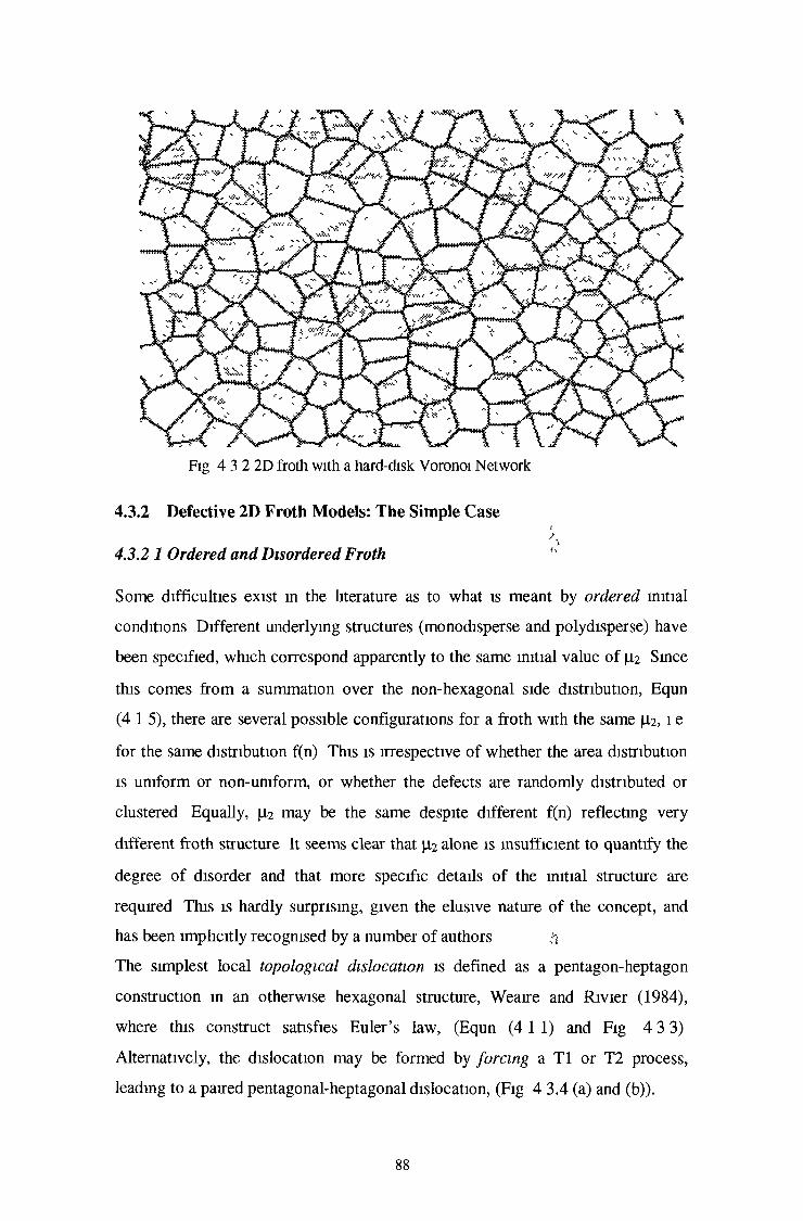
Fig 4 3 2 2D froth with a hard-disk Voronoi Network

4.3.2 Defective 2D Froth Models: The Simple Casei

4.3.2 1 Ordered and Disordered Froth "Some difficulties exist in the hterature as to what is meant by ordered initial conditions Different underlying structures (monodisperse and polydisperse) have been specified, which correspond apparently to the same initial value of (4,2 Since this comes from a summation over the non-hexagonal side distribution, Equn (4 1 5), there are several possible configurations for a froth with the same (1 2 , 1 e for the same distribution f(n) This is irrespective o f whether the area distribution is uniform or non-uniform, or whether the defects are randomly distributed or clustered Equally, (I2 may be the same despite different f(n) reflecting very different froth structure It seems clear that |i2 alone is insufficient to quantify the degree o f disorder and that more specific details o f the initial structure are required This is hardly surprising, given the elusive nature o f the concept, and has been implicitly recognised by a number of authorsThe simplest local topological dislocation is defined as a pentagon-heptagon construction in an otherwise hexagonal structure, Weaire and Rivier (1984), where this construct satisfies Euler’s law, (Equn (4 11) and Fig 4 3 3) Alternatively, the dislocation may be formed by forcing a T1 or T2 process, leading to a paired pentagonal-heptagonal dislocation, (Fig 4 3.4 (a) and (b)).

88

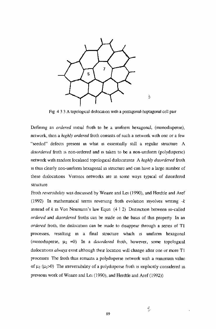
— V 75 \

Defining an ordered initial froth to be a uniform hexagonal, (monodisperse), network, then a highly ordered froth consists of such a network with one or a few “seeded” defects present in what is essentially still a regular structure A disordered froth is non-ordered and is taken to be a non-uniform (polydisperse) network with random localised topological dislocations A highly disordered froth is thus clearly non-uniform hexagonal in structure and can have a large number of these dislocations Yoronoi networks are in some ways typical o f disordered structureFroth reversibility was discussed by Weaire and Lei (1990), and Herdtle and Aref (1992) In mathematical terms reversing froth evolution involves writing -k instead of k in Von Neumann’s law Equn (4 1 2) Distinction between so-called ordered and disordered froths can be made on the basis of this property In an ordered froth, the dislocation can be made to disappear through a series of T1 processes, resulting in a final structure which is uniform hexagonal (monodisperse, (0,2 =0) In a disordered froth, however, some topological dislocations always exist although their location will change after one or more T1 processes The froth thus remains a polydisperse network with a minimum value of (j-2 (jll2>0) The irreversibility o f a polydisperse froth is implicitly considered in previous work of Weaire and Lei (1990), and Herdtle and Aref (1992))

Fig 4 3 3 A topological dislocation with a pentagonal-heptagonal cell pair

89

7 X I

T V 7

(a)

Fig 4 3 4 (a) (b) A topological dislocation ,(a) with pentagonal-heptagonal cell pairs formed by a T1 process,(b) with a pentagonal-octagonal cell formed by a T2 process

From these definitions o f order and disorder, it seems clear that Smith (1952) described a highly disordered system whereas Aboav (1980) mvestigated one which was highly ordered m that its underpinning was the hexagonal form. Both ordered and disordered initial conditions were considered m Glazier et al (1990) whereas Weaire and Lei (1990) discussed disordered systems only Investigations of froth behaviour when a smgle defect is present m a highly ordered system are due to Levitan (1994), Ruskin and Feng (1995) We consider details of froth evolution for a range o f different initial conditions in what follows

4.3.2.2 Single Defect 2D Froth Model,1The question of initial conditions was raised m earlier work cited above It is

known that a system with only hexagonal patterns is m full equilibrium with regard to diffusion, l e a perfect ordered froth However, it is o f mterest to examine quantitatively the mtroduction of disorder mto such a system. We consider initially the smgle defect case

90

The initially transient behaviour of a relatively ordered froth has been interpreted in terms o f the growth of individual topological defects The study of this growth was first taken up by Levitan (1994), who considered the insertion of a single such defect into a froth of hexagonal cells He used an approximation which is attractive in that it offers the potential to simulate larger, closer-to-asymptotic systems, but results obtained were in disagreement with previous tentative conclusions, (Wearre in Blackman and Taguena (1989)) We have re-examined this problem by direct simulations which are more extensive than those previously undertakenLevitan’s method first forces a T1 topological process, to take place in a group of cells and follows this with a T2 process, for which the probabilities of a triangle, square and pentagon being formed are the same In fact, the first T1 process gives rise to two five-sided cells and two seven-sided cells in the network, (Fig 4 3 4(a)) Levitan used a mean field theory to show that the topological distribution associated with a single defect approaches a fixed asymptotic form, with a high peak f(6) = 0 6 This implies that |J.2 attains a different and stable value in conflict with previous predictionsWe have implemented a 2D dry froth with a single topological defect, based on a perfect hexagonal network to ensure correspondence with Levitan’s original construction The defect is based on a symmetrical arrangement of two pairs of pentagonal and heptagonal cells with minor discrepancies m the areas of the component cells and with all hexagonal cells surrounding the defect having the same area, (Fig 4 3 4(a)) Additionally, we consider another type of topological defect, where the distortion is achieved by suppressing an edge in the original network giving an eight-sided cell with two symmetrical five-sided cells amongst its nearest neighbours (Fig 4 3 4(b)) We have also used another ordered construction to create a third kind of defect, in which the areas of the defect and its neighbouring cells have been adjusted, (detailed Figs are shown in Appendix C) Periodic boundary conditions are used but, for convenience, the defective cell is centrally placed in the network, smce the system is size limited, so that we can monitor the evolution for as long as possible Calculations are not pursued beyond the stage where the defect impacts on the boundary

91

4.3.3 Multiple Defects in an Ordered / Disordered FrothA froth with multiple defects is an extension of the single defect example where now increased amounts o f disorder are considered to be introduced into the initial hexagonal network We also consider initial structures for the froth network which are both ordered and disordered (p89) before insertion of the defects Direct simulation is again used to investigate froth evolution for different system sizes and initial set-ups in order to obtain information directly on each time step during the whole evolution Defects which are sparse in the froth as a whole evolve naturally before impacting on each other after a long period o f time We consider systems of size up to 1600 cells and initial structures which range from highly ordered to highly disordered

f

4 3.3.1 Multiple Defects in an Ordered FrothFrom our definition, an ordered froth is based on the hexagonal network, where for any value o f n, all cells have roughly the same initial area For a highly ordered hexagonal network, we have introduced a number o f defects, d, as a pair of pentagon-heptagon dislocations,(i) d=4 in a system of size 400 cells (|i2=0 05),(u) d = l in a system of size 900 cells, (|i2 ~0 03),For a hexagonal network with low order, we have introduced,(m) d=30 m a system of 400 cells, (|i2 =0 3),(iv) d=60 in a system of 900 cells (|i2 =0 27)

4 3 3.2 Multiple Defects in a Disordered Frothsij

In a disordered froth normally obtained from the Voronoi network, the area of an n- sided cell may vary considerably and |U2 provides an indicator o f the degree and nature of disorder arising from increased dispersion in f(n) For a highly disordered froth, we have considered the evolution of(v) a system of 900 cells with initial JU2 =1 2,(vi) a system of 1600 cells with initial |i2 =1 6, (f(4)=0 12, f(5)=0 25, f(6)=0 28,

f(7)=0 09, f(9)=0 02, f(10)=0 01)

92

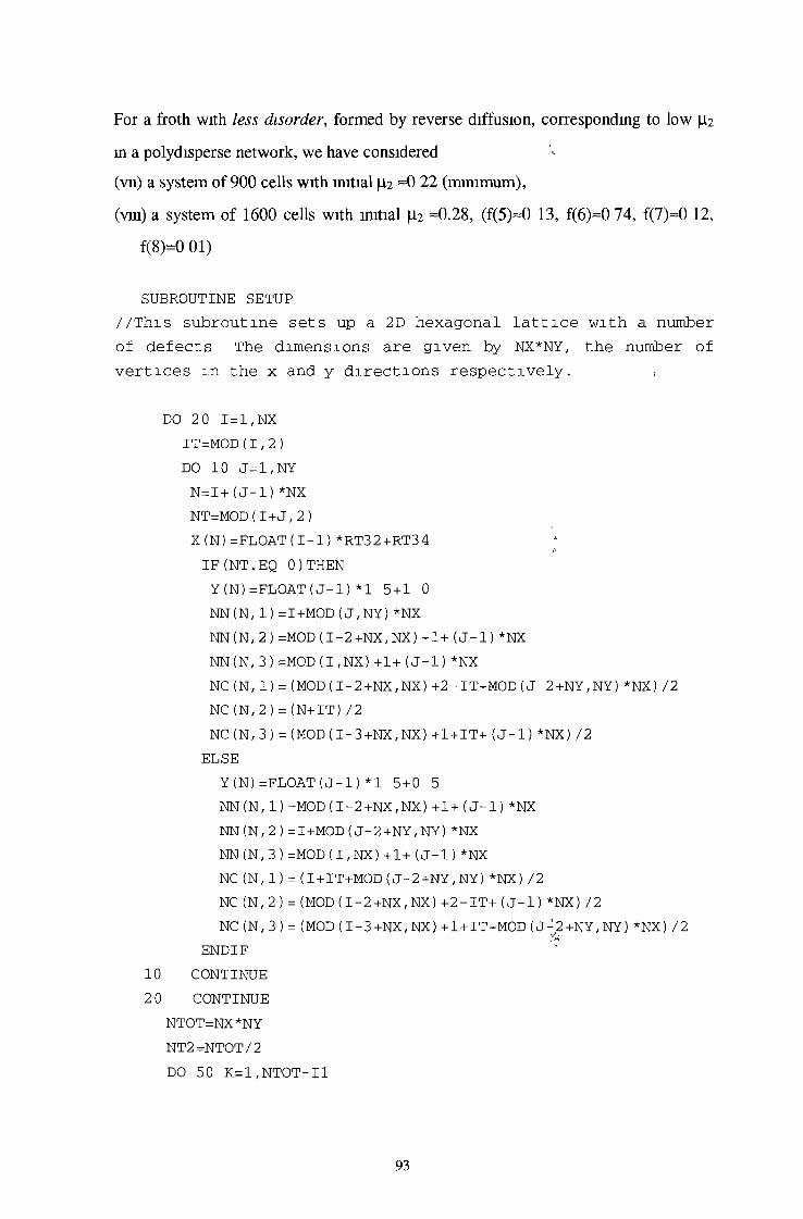
in a polydisperse network, we have considered(vu) a system of 900 cells with initial [4,2 ~0 22 (minimum),(vrn) a system of 1600 cells with initial \h =0.28, (f(5)=0 13, f(6)=0 74, f(7)=0 12,

f(8)=0 01)

SUBROUTINE SETUP //This subroutine sets up a 2D hexagonal lattice with a number of defects The dimensions are given by NX*NY, the number of vertices m the x and y directions respectively. ,

DO 2 0 1=1,NX IT=MOD(1,2)DO 10 J =1,NY N=I+(J-l)*NX NT=MOD(1+J,2)X(N)=FLOAT(1-1)*RT32+RT34 j*IF(NT.EQ 0)THEN Y (N)=FLOAT(J-1)*1 5+1 0 NN(N,1)=I+MOD(J,NY)*NX NN (N, 2 ) =MOD (1-2 +NX, NX) +1+ (J-l) *NX NN(N,3)=MOD(I,NX)+1+(J-l)*NXNC(N,1) = (MOD(1-2 +NX,NX)+2-IT+MOD(J-2+NY,NY)*NX)/2 NC(N,2)=(N+IT)/2NC(N,3) = (MOD(1-3 +NX,NX)+1 + IT+(J-l)*NX)/2 ELSEY (N)=FLOAT(J-l)* 1 5 + 0 5 NN(N,1)=MOD(I-2+NX,NX)+1+(J-l)*NX NN(N,2)=I+MOD(J-2+NY,NY)*NX NN(N,3)=MOD(I,NX)+1+(J-l)*NX NC(N,1)=(I+IT+MOD(J-2+NY,NY)*NX)/2 NC (N,2) = (MOD(1-2 +NX,NX)+2-IT+(J-l)*NX)/2 NC(N,3)=(MOD(I-3+NX,NX)+1+IT+MOD(J-2+NY,NY)*NX)/2

END IF 10 CONTINUE 2 0 CONTINUE

NTOT=NX*NY NT2=NTOT/2 DO 50 K=l,NTOT-Il

For a froth with less disorder, formed by reverse diffusion, corresponding to low \ii

93

DO 51 J=1,3IF(NN(K,J).GE.Nl.AND.NN(K,J).LE N2)THEN NN(K,J)=NN(K,J)-1

ELSEIF(NN(K,J) GT N2)THEN NN(K,J)=NN(K,J)-2

ELSEIF(NN(K,J).EQ.N2.AND.K.LT (N2-1))THEN NN(K,J)=NN(K,J)-1

ELSEIF(NN(K,J) EQ N2 AND K GE.(N2-1))THEN NN(K,J)=NN(K,J)-2

END IFIF(NC(K,J).GE,N3)THEN NC(K,J)=NC(K,J)-1 END IF

51 CONTINUE 50 CONTINUE

NTV=NTOT-11 12=11/2 NTC=NT2-I2

DO 3 0 K=1,NTOT IVLIST(K)=K

3 0 CONTINUERT32=RT32*3.0 DO 40 K=1,NT2

ICLIST(K)=K NCELL(K)=6 VOL(K)=RT32 P(K)=0 0

40 CONTINUE NCELL(435)=7 NCELL(466)=7NCELL (436) =5 'fNCELL(465)=5RS1=(SQRT(10.0)-2 )/2.VOL(435)=RT32+RT34 VOL(436)=5*RT34 VOL(465)=RT32-RT34 VOL(466)=RT32+RT34 X(931)=X(931)+0.5*RT34 Y(931)=Y(931)+5./8.X (932)-X(932)-0 5*RT34 Y(932)=Y(932)-5./8.

94

END IFR ETURNEND

We give detailed results for some of these models in the next Section as examples An example is also shown on the diskette in Appendix E

4.4 Results and Discussion

4.4.1 Voronoi Disordered Froth4.4.1.1 Additional Notes on Direct Simulation Implementation- PerformanceFor direct simulation, it is possible to specify the precise geometrical description of the structure and its evolution We note that Kermode and Weaire (1990) used the routines F04ARF and F04ATF in the NAG library to solve the matrix equation, but these are not available in the NAG library version available on the VAX cluster in DCU We have, therefore, modified the programme by using instead the Gauss method The external library CALCOM is also unavailable, so that for the current preliminary studies we have omitted the 2D-Froth graph plotting routine and substituted our own, written in C A copy o f this program is given on diskette together with 2D-Froth program in Appendix E For the largest system considered size 3000 cells with initial disordered Voronoi network set-up, the volume of information to be stored is considerable and run tunes are of the order of several hours for each stage o f the simulation due to the large number of complicated network checks and continuously iterated calculations A 3000-cell system appears to be the practical limit for the computing power o f the hardware configuration that we have used for this sequential approach For 1000 and 3000 cell systems, the first runs required more than 5 and 12 hours respectively, and succeeding runs about 2 and 7 hours on the VAX cluster available in DCU We concentrate on specific distributions of interest in what follows “The tune steps are small in our simulation so that it is easy to observe detailed topological distributions and related behaviour exactly for each step Here the number of tune steps relates to the number o f diffusion and equilibration

95

processes which have taken place, with the evolution time, T, measured in units of <AQ>/k, where < A0> is the initial average area over all cells, and k is the constant in Von Neumann’s Law, and may be arbitrarily chosen, (Kermode and Wearre(1990)) i

4.4.1.2 Results o f Froth Simulation

We examine the distributions o f number o f sides and area, and the respective correlations For the systems of 1000 and 3000 cells, we obtain the values of the second moment, |i2 =1 5 and ^ =1 63 respectively, where the later one is highcompared to values quoted by previous authors with the exception of Wejchert et al (1986) This in part may be ascribed to the much larger network, so that more cells are involved in a knock-on effect from a given topological change and partly to a choice of different scale factors and hence the handling o f small cells as noted earlier, (Section 4 2 3 2) Nevertheless, clear equilibrium behaviour is established In Fig 4 4 1-2, the distribution functions f(n) and the second moment, |i2, for a system of 3000 cell are shown Equn (4 1 2) suggests that the,rate of area change is the same for all n-sided cells, irrespective o f the nature o f neighbouring cells In a real system, the large cells are more likely to touch the boundary o f a finite area than the small cells, so that we have a systematic bias against the inclusion of very large cells in our distribution function Also, we know that rate o f growth of a cell is dependent on its shape, l e is only affected by the number o f sides o f the original cell configuration Therefore, it is unnecessary to calculate all the side lengths and sum the diffusion across each side in order to determine the rate of growth for a cellWe have also looked at the correlations between area or diameter, <An>, (or d),and number o f sides, n, (Lewis’s Law), and correlations between n and m(n), the number of sides of neighbouring bubbles, (Aboav-Weaire law) Results are shown in Figs 4 4 3-4 For the former, we expect a linear relation between the cell area and the number o f sides, where <An> and n are recorded at various stages during

'"I’I?the evolution of the soap froth Agreement is obtained with Lewis Law, also with the Aboav-Weaire Law, but a is not normally quoted values o f 1 or 1 2, (a = 0 7)

96

the

seco

nd

mom

ent

Also deviations from Lewis Law appear to be more marked for the smaller system, 1 e system size of 1000, although departure from linearity is small

0 4

0 3

S O 2

0 1

0

Fig 4 4 1 side distribution f(n) vs side No n m a system of size 3000

2

1 5

1

0 5

01 2 3 4 5 6 7 8 9 10 11 12

T

Fig 4 4 2 the second moment, \x,j vs T4 5

43 5

3c 2 5 < 2

1 5 1

0 50

1

Fig 4.4 3 Lewis Law for a system of size 3000

97

60

10 --

0 -I 1------------ 1------------ 1------------ 1------------ 1------------3 4 5 6 7 8 9

n

Fig 4 4 4 Aboav-Weaire Law for a system of size 3000

Precise geometrical description o f the structure and evolution of the froth are presented m an example given in Appendix D for a system of size 900 We have extended such calculations to hundreds or even thousands o f cells, and obtamed results from the simulations which show that scaling laws durmg the evolution of a froth are m reasonable agreement with experiment, and previous simulation studies

4.4.2 Froth with a Single Defectjift

We have implemented the froth with a single defect, (Fig 4 3 3 and Appendix C), for systems of size 100, 400 and 900 cells respectively We give details of the results for a system o f size 400 cells as an example Similar results are found for all system sizes usedIf we define an approximately circular “front” o f disturbance surrounding the large defective cell and mcludmg cells which have undergone a single topological change, the circular “front” will mclude these (plus other cells which impmge on the circle m part, but which have not yet undergone change) Levitan (1994) similarly defmes a “cluster”, which refers to the “front” used in our simulations plus a boundary of hexagonal cells The slight modification we have used does not affect the behaviour of |i2, or the side distribution but enables us to consider separately (4,2 in the frontFigs 4 4.5 show the evolution withm the front at specific time, steps for different initial defect types, corresponding to Fig 4 3 4(a) We can see that the number of

area of the disturbance For the defect formed by edge suppression, starting from the ordered non-Voronoi network set-up (see Fig 4 3 4(b)) and ordered Voronoi network (see Appendix C), we have observed very similar behaviour in the froth evolution We give detailed results for the initial structure shown in Figs 4 3 3 (a)

5and (b) as follows -

99

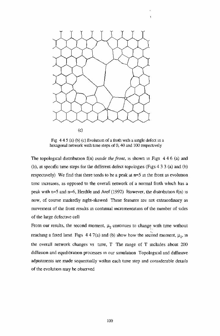
(c)Fig 4 4 5 (a) (b) (c) Evolution of a froth with a single defect in a

hexagonal network with time steps of 0 ,4 0 and 100 respectively

The topological distribution f(n) inside the fron t, is shown in Figs 4 4 6 (a) and (b), at specific tune steps for the different defect topologies (Figs 4 3 3 (a) and (b) respectively) We find that there tends to be a peak at n=5 in the front as evolution time increases, as opposed to the overall network of a normal froth which has a peak with n=5 and n=6, Herdtle and Aref (1992) However, the distribution f(n) is now, of course markedly right-skewed These features are not extraordinary as movement of the front results in continual incrementation of the number of sides of the large defective cellFrom our results, the second moment, |0,2 continues to change with tune without reaching a fixed limit Figs 4 4 7(a) and (b) show how the second moment, |i2, in the overall network changes vs time, T The range o f T includes about 200 diffusion and equilibration processes m our simulation Topological and diffusive adjustments are made sequentially within each time step and considerable details of the evolution may be observed

100

n

(a)

n

(b)Fig 4 4 6(a) (b) Topological distribution f(n) in tht front with time step of 60(A), 120(0), and 160(o) Initial set-up Fig 4 3 3 (a) (b) respectively

Fluctuations in the value of |0,2 around the underlying trend can be explained directly in terms of the T1 and T2 processes, with a high \i2 corresponding to the defect surrounded by a number o f three- or four-sided cells, and a sudden decrease in |i2 associated with the disappearance o f one of these cells During growth in area of the defect, \ii keeps a relatively stable value until the next T1 occurs Clearly, as more cells are involved in the evolution and the number of sides o f the defect increases, the value of \i2 overall changes more rapidly and is dominated by the contribution of the defective cell Over the whole range o f T, (0-2

~ T appears to describe the observed behaviour, with (3 >1 However, few changes take place initially, relative to the evolution as a whole, and for the upper range o f T, ¡12 vs T is roughly linear, although it is not clear that a true asymptote is attained

101

T

(a)

T

(b)Fig 4 4 7(a) (b) p.2 in the overall network vs time T for a froth of

400 cells Initial set-up Fig 4 3 3 (a) (b) respectively

For a simple theoretical model o f a large defect with N sides surrounded by N small cells, newly converted side lengths of the small cells will be characteristic of the whole network, 1 e N ~ A(d)°5, with A(d) the area o f the defect Then, m the asymptotic limit, Von Neumann’s law becomes dA(d)/dt = kA(d)05, 1 e A(d) ~ T Similarly, in the front, the topological distribution will be dominated by the defect, so that |12 (d) ~ N2 with N ~ T, 1 e (-I2 (d) ~ T2Furthermore, the defect gradually mvolves more and more cells m the overall network, so that asymptotically the exponents for the front and the overall network should be the same From our simulations, we find fo r the defect that A(d) mcreases with T at the expense o f other cells distorted by topological changes If we define the mcreased area AA(d) = A(d) - A(d)0, where A(d)0 is the

102

original area of the defect, for the defect formed by edge suppression, e g Figs 4 3 3(b), we obtain roughly AA(d) ~ T2 after the initial period of evolution, with the radius o f the rough perturbation circle, r ~ T approximately, Figs 4 4 8 (a) and (b) illustrate for the set-up of Fig 4 3 3 (b) Furthermore, we find that |J,2 (d) changes roughly linearly with the average intercept, <d>, where <d> equals the square root of the average cell area in the front, Fig 4 4 9

(a)

(b)Figs 4 4 8 (a) (b) Increase m defective area AA(d) vs time, T, for a froth of 400 cells Initial structure Fig 4 3 3 (a) and (b) respectively

Fig 4 4 9 112(d) m the front vs average intercept, <d>

103

It seems clear that the behaviour of a froth with a single defect in a uniform hexagonal network does not lead to a normal scaling state as found for the nondefective froth by numerical simulation and as predicted by theory We find that f(n) in the front tends to develop a long tail extending to large values o f n and with a peak at n=5 This is in agreement with Aboav (1980), who also quotes a =2 for the area growth exponent However, the suggestion that \i2 overall varies linearly with time (comment by Weaire and Kermode (1983a) on Aboav’s work), is not wholly supported by our findings and is in conflict with the predictions of the simple model It is only with hindsight that it has been suspected that Aboav was dealing with a transient system with defects, characterised by different values of the growth exponents Our own results are probably not in the asymptotic region since the maximum number of sides achieved by any defect is N=44 at the late stage. Nevertheless, they are supported by recent work o f Jiang et al (1995)In summary, we find that there is some similarity between the behaviour of our system and that of Levitan (1994), but we do not agree with a fixed form for f(n) as obtained by Levitan The value o f \x,2, whether for the front or for the overall network, does not reach a steady-state after initial fluctuations at this system size, unlike normal froth evolution

4.4.3 Monodisperse and Polydisperse4.4.3.1 Results and DiscussionSimilar behaviour is observed for initial conditions noted in section 4 2 3, for example (1) and (n), and also for example (m) and ( iv ) , results are thus discussed in detail for (n) and (iv) onlyFor the ordered froth, (defined p89), the side distribution, f(n), is illustrated in Figs 4 4 10 (a) and (b) for specific time steps Since a single time step consists of the number o f diffusion and equilibrium processes which have occurred, the evolution time, t, is measured in units o f <A0>/k, as previously with k a constant defined in Equn (4 1 2) The second moment, [i2, vs time and the average area, <A> vs time are shown in Figs 4 4 11-12 Agreement with the Aboav-Weaire law is shown in Fig 4 4 13, where a is approximately constant (a ~ l 05)

104

(a)

n

(b)Fig 4 4 10(a) (b) The side distribution, f(n) at time steps of 0, 120, 260 for a highly (n) and a low ordered froth ( iv), the heavier dark line represents f(n) in the quasi-scaling scaling state

(a)

105

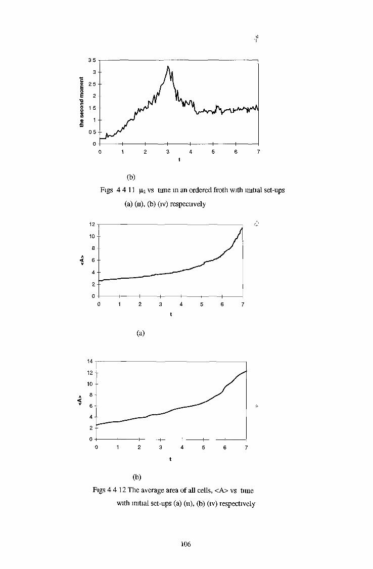
<A>

the

seco

nd

mom

ent

t

(b)Figs 4 4 11 (i2 vs tune in an ordered froth with initial set-ups

(a) (11), (b) (iv) respectively

(a)

t

(b)Figs 4 412 The average area of all cells, <A> vs time

with initial set-ups (a) (11), (b) (iv) respectively

106

8 4 A7 A A6-- ^ 4 4 « i i

c 5 - E 4 -

3 --2 --1 --0 -I 1------ 1-------1-------1------

0 3 6 9 12 15n

Fig 4 4 13 Aboav-Weaire Law m a low ( -A ) and highly (0) ordered frothIf considering the alternative illustration, l e nm(n) vs n (as shown in Fig 4 4 4), the line corresponds to constant a -1 05

For a highly ordered froth, we observe that the side distribution f(n) is markedly right-skewed with the long tail reflecting the presence of many-sided cells, (Fig 4 4 10(a)) The second moment grows indefinitely with time, |i2 ~t, as a result, (Fig 4 4 11(a)) Therefore, if the system size is large enough, we expect that |i2

will continue to increase as larger many-sided cells are formed Our findings for [Lz vs t and also for the average area of all cells <A> ~ t “, a =2 are in agreement with those of a single defect as discussed in Section 4 4 2The scaling state is reached when both f(n) and \i2 attain time-invariant values and obviously does not apply for a highly ordered froth, where neither f(n) nor \±2 tend to a fixed form However, if we truncate f(n) at n = n *, (n* < 12), we find that the side distribution f(n*) is effectively fixed after the initial period of evolution, (see e g Fig 4 4 10(a), f(4)=0 08, f(5)=0 37, f(6)=0 35, f(7)=0 09) Such a froth may be said to be in a quasi-scaling state, although clearly \iz for all n continues to increase This suggests, additionally, that a more appropriate measure of the froth structure might well be the third or fourth moment of the distribution, f(n)The emergence of a quasi-scaling state in the highly ordered froth, however, does not tend to wholly support the view that Aboav’s results describe a transient stage, but requires focus on the later time-evolution, which is not provided. In fact, ten percent of the initial 5000 cells remained for the value of \iz given in this work, Aboav (1980) An alternative explanation, that the long-term evolutionary behaviour of a highly ordered froth reaches partial equilibrium at best, obtains

9 -|------------------------------------------------------------------------------

107

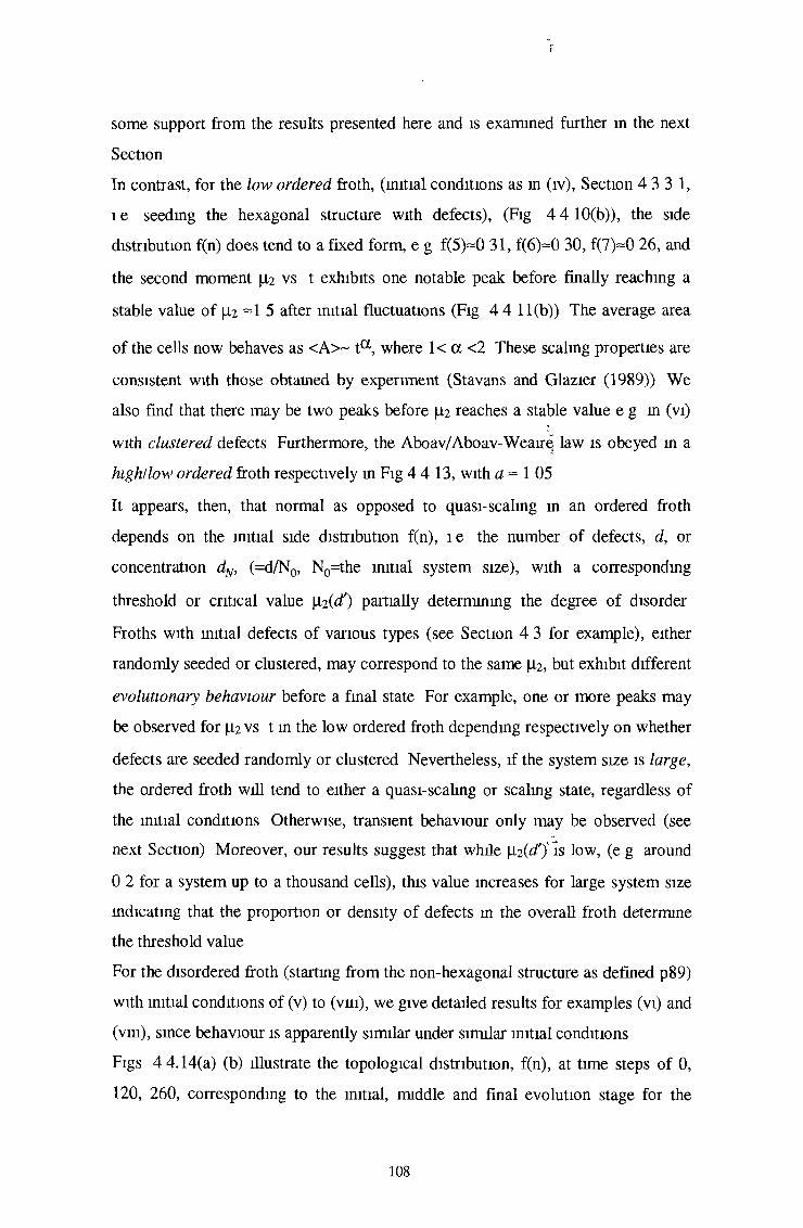
some support from the results presented here and is examined further in the next SectionIn contrast, for the low ordered froth, (initial conditions as in ( i v ) , Section 4 3 3 1, 1 e seeding the hexagonal structure with defects), (Fig 4 4 10(b)), the side distribution f(n) does tend to a fixed form, e g f(5)=0 31, f(6)=0 30, f(7)=0 26, and the second moment |J,2 vs t exhibits one notable peak before finally reaching a stable value of [iz ~1 5 after initial fluctuations (Fig 4 4 11(b)) The average areaof the cells now behaves as <A>~ ta , where 1< a <2 These scaling properties are consistent with those obtained by experiment (Stavans and Glazier (1989)) We also find that there may be two peaks before |J,2 reaches a stable value e g in (vi)

1with clustered defects Furthermore, the Aboav/Aboav-Weaire law is obeyed in a high/low ordered froth respectively in Fig 4 4 13, with a ~ 1 05 It appears, then, that normal as opposed to quasi-scaling in an ordered froth depends on the initial side distribution f(n), le the number of defects, d, or concentration dN, (=d/N0, N0=the initial system size), with a corresponding threshold or critical value \x,i(d') partially determining the degree of disorder Froths with initial defects of various types (see Section 4 3 for example), either randomly seeded or clustered, may correspond to the same |J,2, but exhibit different evolutionary behaviour before a final state For example, one or more peaks may be observed for |i2 vs t in the low ordered froth depending respectively on whether defects are seeded randomly or clustered Nevertheless, if the system size is large, the ordered froth will tend to either a quasi-scaling or scaling state, regardless of the initial conditions Otherwise, transient behaviour only may be observed (see next Section) Moreover, our results suggest that while ¡iiid'j'is low, (e g around 0 2 for a system up to a thousand cells), this value increases for large system size indicating that the proportion or density of defects in the overall froth determine the threshold valueFor the disordered froth (starting from the non-hexagonal structure as defined p89) with initial conditions of (v) to (vrn), we give detailed results for examples (vi) and (vm), since behaviour is apparently similar under similar initial conditions Figs 4 4.14(a) (b) illustrate the topological distribution, f(n), at tune steps of 0, 120, 260, corresponding to the initial, middle and final evolution stage for the

108

disordered Yoronoi structure Figs 4 4 15-16 show how the second moment |i.2 andi

average area <A> change with time for examples (vi) and (vm) respectively For the correlation laws, e g the Aboav (Aboav-Weaire) law, we found that the constant a does not have the value of 1 or 1 2 as for the normal case, but has a different value of a ~ 0 6~0 7 roughly, shown in Fig 4 4 17

n

(a)

n

(b)Figs 4 4 14 The side distribution, f(n) at time steps of 0, 120, 260 for

(vi) a high disordered and (vm) a less disordered froth, the heavier dark line represents f(n) m the scaling state

109

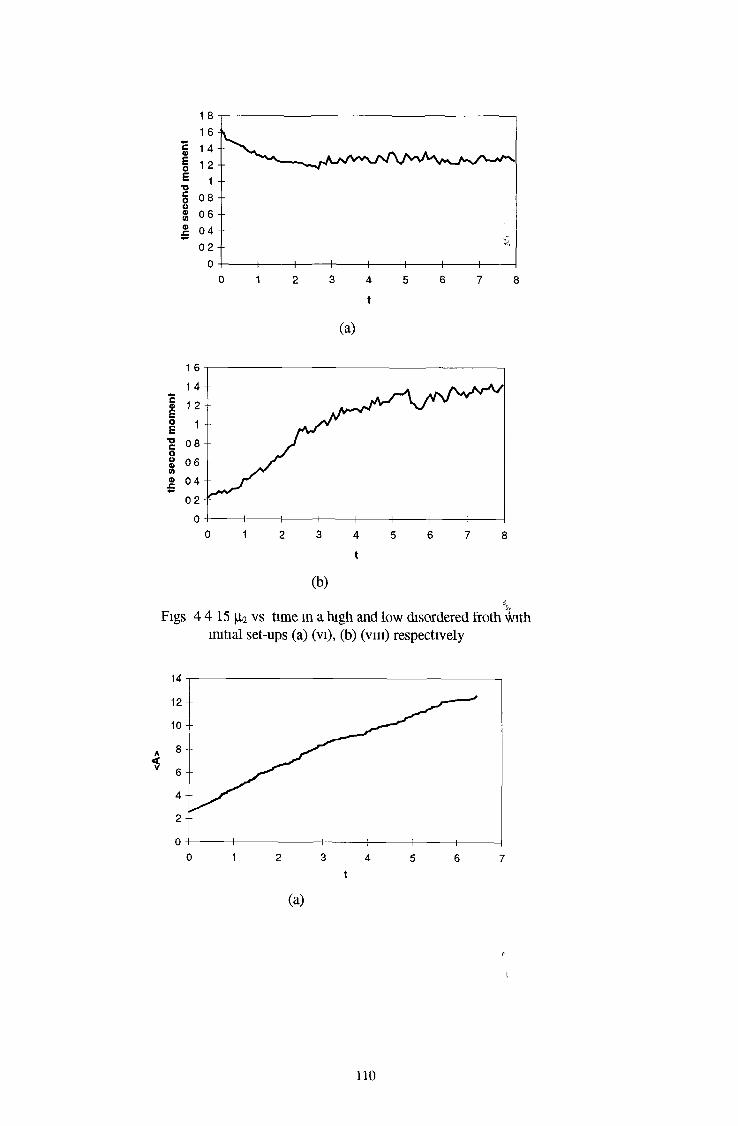
the

seco

nd

mom

ent

(a)

(b)Figs 4 4 15 |i.2 vs time in a high and low disordered froth with

initial set-ups (a) (vi), (b) (vm) respectively

t

(a)

110

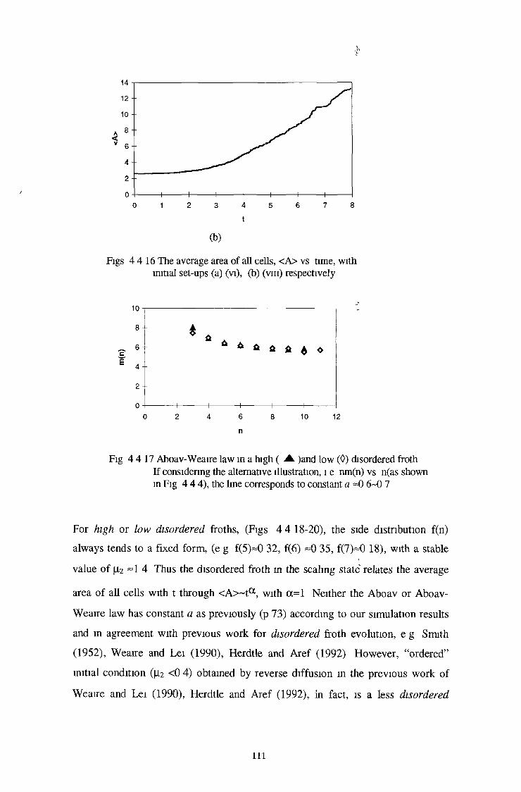
J1

t

(b)Figs 4 4 16 The average area of all cells, <A> vs time, with

initial set-ups (a) (vi), (b) (vm) respectively

n

Fig 4 4 17 Aboav-Weaire law in a high ( A )and low (0) disordered froth If considering the alternative illustration, l e nm(n) vs n(as shown in Fig 4 4 4), the line corresponds to constant a =0 6~0 7

For high or low disordered froths, (Figs 4 4 18-20), the side distribution f(n) always tends to a fixed form, (e g f(5)=0 32, f(6) =0 35, f(7)=0 18), with a stable value of ¡12 ~1 4 Thus the disordered froth in the scaling state relates the averagearea of all cells with t through <A>~ta , with a = l Neither the Aboav or Aboav- Weaire law has constant a as previously (p 73) according to our simulation results and in agreement with previous work for disordered froth evolution, e g Smith (1952), Weaire and Lei (1990), Herdtle and Aref (1992) However, “ordered” initial condition (|j,2 <0 4) obtained by reverse diffusion in the previous work of Weaire and Lei (1990), Herdtle and Aref (1992), in fact, is a less disordered

111

structure by our definition The semantic distinction here, can be confusing, but relates to whether the original structure can be defined as ordered (in the sense of p 89) or disordered A good definition remains elusive1Consequently, our results support the existence of a universal scaling state, irrespective of system size, for a disordered froth, based on a Voronoi construction We find that (I2 vs t has either a lower peak value, (¡12 <2 0), than that observed for an ordered froth (Fig 4 4 15(b)) or increases monotomcally (Fig 4 4 19(b)) While there appears to be agreement as to the location of the \x,2 peak during ordered and disordered froth evolution, it seems likely that it is merely a coincident surface phenomena since the peak values are different (For example, we obtain a high peak, (such as (12 >3 0) for the ordered froth, (under condition(iv)), whereas for the disordered froth we observe either a small peak (|i2 <2 0) or none) This agrees with former work, Stavans and Glazier (1989), and Weaire and Lei (1990), where |i2 was found to rise rapidly to a maximum (|i2 =2 65 and |i2

=19 respectively), then dropped to the constant value (12 =1 4 Furthermore, the phenomenon of more than one peak for ¡12 vs time (see Glazier et al (1990)), appears to be a peculiarity of the ordered froth and we find no evidence for multiple peaks for any disordered system we have simulated

4.4.3.2 Conclusions on Single/Multiple Defect(s)For a froth with a single defect, our results for the behaviour of the front are in agreement with the original experimental work of Aboav (1980), and indicate that a different scaling relation applies in an ordered froth, (1 e a quasi-scaling state at best) Regardless of the defect type and initial configuration, for a single defect, d= 1, there are some grounds for supporting the suggested system behaviour put forward by Levitan (1994), but the overall results are in conflict with his predictions for the quantities characterising the long-term evolution For a froth with multiple defects, <¿>1, we have reconciled apparent discrepancies in the scaling properties describing the froth evolution In particular, our findings support the view that again a quasi-scaling state at best is achieved in a highly ordered froth, where the side distribution, f(n*) (n*<12) tends to have a fixed form whereas f(n) for all n has long tail corresponding to the unlimited growth of [I2. These

112

remarks must be qualified of course by noting that only finite systems to moderate size can be simulated directly A universal scaling state is, however, attained for both the disordered and low ordered froth, where f(n) has a fixed form corresponding to a system-invariant asymptotic value of ju.2 =14 Additionally, we offer an alternative explanation on the early result of Aboav(1980) indicating that the ordered froth may progress beyond transience or, alternatively, exhibits a prolonged transient region This is further discussed in what follows We also find that the Aboav (or Aboav-Wearre) law has different values of constant a in the ordered and disordered froth

4.4.4 A Note on Stages of Evolution in a 2-D FrothFrom the above, it appears that the evolutionary process of 2D froth consists of two regions involving several distinct stages, which are characterised by the froth structure In particular, transient behaviour which reflects initial levels of froth disorder can be varied both in its nature and duration The final stage of froth evolution is associated with a few remaining bubbles, which change relatively slowly, unlike the many, frequent changes originally associated with transience Thus, late configurations do not affect achievement of scaling, but influence the rate at which it is attainedThe studies of ordered 2-D froths with single/multiple defects provide some examples for length of transition period, which appears! to be related to concentration of defects, and highly ordered systems with few defects exhibit an anomalous approach to the scaling state The question of the way in which these factors influence the length of the transient and other stages is discussed here In many areas of statistical physics, the evolutionary time T—» as N—> °°, butscales are not interchangeable, since two distinct regions are involved, (a) 1 « T « T(N), and (b) T » T(N), where for some T > T(N), finite size-effects operate This is demonstrated also in zero-temperature simulations of Potts models, Derrida et al (1996), which may be relevant to recent bubble growth experiments, Tam et al (1997) Consequently, any discussion of froth evolution must include behaviour in both regions (a) and (b)

113

The key factor in transience, as originally described, appeared to be that the early evolution in region (a) involved a large number of bubbles in topological changes, producing considerable variation in the form of f(n) and value of |li2 Actual time taken is thus dependent on system and simulation characteristics are difficult to quantify precisely Clearly, as the number of bubbles decreases, the sizes of the remainder tend to increase so that the number of bubbles remaining, (or "survivors" - expressed as a percentage of the initial number), is then crucial as an indicator of the potential for further change and in the determination of T(N) For a large system where scaling is achievable, transient effects would normally be expected to occur for a relatively large number of survivors, le T « T(N) However, defects are known to affect the nature of transient behaviour It seems clear, therefore, that duration of any stage in the froth evolution depends on the concentration of defects and their distribution, (whether clustered or random) Some illustrative evidence can be provided in support of this view as follows For a random Voronoi structure used as a sample of disordered froth, early numerical studies for very small system size (N=100) recorded initially rapidly changmg behaviour, even though scaling could not be observed, Weaire and Kermode (1983b) This is due to the fact that the transient effects are rapidly overtaken by the finite size of the system In subsequent studies on larger systems of several hundreds of bubbles, the nature of the early evolution was variable but a unique final state was achieved with a fixed form side distribution, corresponding to a stable value of |i2, irrespective of the amount of disorder in the initial frothstructure, Weaire and Lei (1990), 1 e the scaling state was observed, (region (a) as usual) However, this result does not hold for special cases of disorder, e g the occurrence of a single defect in an otherwise ordered froth, where the scaling state is not observed at all for moderate system size (See section 4 4 2 earlier)In an ordered froth, the behaviour varies considerably with the number of defects introduced The anomalous case for a single initial topological dislocation reduces evolution of the froth to that of a single large bubble or single compound bubble cluster, which proceeds to grow until the froth is consumed Thus |i2 for the wholesystem grows indefinitely with tune, (region (b)) The nature of the initial topological dislocation is reflected in the configuration achieved by the froth in the

114

final stages of evolution, (examples are given in Ruskin and Feng (1995)) However, the side distributions f(n) are similar except for the presence of several large bubbles, (forming a compound cluster in the dislocation caused by a T1 process), which have the effect of reducing the extreme skew in f(n) Furthermore, for few defects, an intermediate stage in region (a) is observed, which neither reflects the many, rapid changes associated with transience nor the final fixed value of scaling This "quasi-scaling" or slow approach to true scaling, has been noted for moderate system size, (N=400), and is characterised by a relatively stable "local pattern”, with fixed side distribution f(n*) and |i2 (n*) f°r n*<12, see Section 4 3 3, Fig 4 4 18 shows |X2(n*) vs survivor percentage for one defect

survivor percentage

Fig 4 4 18 The local second moment, p2(n*) vs survivor percentage for one defect For increased disorder, the number of defects (d > 2), or concentration of defects,dN, (=d/N0, N0=the initial system size), determine transient characteristics, (region

h(a)) For a large, initially ordered, system with d or dN small, (and defects clustered), the situation is essentially similar to that of the one defect case, although more large bubbles in the compound cluster imply further limitation on the skew in f(n) For randomly seeded defects, the growth of (i2 continues unchecked until such time as the growth of one defect impinges on another, when it slows down An intermediate stage is again observed with stable |H2(n*), (=0 76,e g for N0 =900 with d=4), attained early in the evolution, despite |i2 increasing For a system which is sufficiently large, the evolution will still achieve equilibrium, (region (a)) for dN small Thus |i2 would be expected to reach its peak

115f

value and start to decrease at a rate which depends on the system characteristics-iTo some extent, this argument is supported by results obtained for a system of

N0=40,000 bubbles with d=500 defects (dN =0 0125), Levitan and Domany (1996) A protracted intermediate period again appears to be a feature of the low concentration of defects since the authors found that, from 40,000 to 1000 bubbles, (0 025N0), the second moment, \l2, continued to grow, whereas from around 600 bubbles to 200 bubbles remaining, (0 015N0 to 0 005N0), 1i 2 decreased and a stable value was obtained Here, all the evolutionary period, prior to obtaining a fixed value for 1i 2 is described as transient, even though it is clear that the percentage of bubbles remaining to take part in topological changes, is very small, so that finite size effects might be expected to operate here, (T —> T(N)) It seems likely that the increase in overall |i2 therefore predominantly reflects a large number of changes for relatively few large bubbles It is arguable whether the transient period should thus be defined as time taken to reach the point at which \i2 shows no further increase, (apart from local fluctuations) or, strictly, as the time taken for fi2 toreach a fixed final value Either definition allows for early stage anomalies such as those found for the final case considered below, but fails to provide much information on changes in the internal froth structureFor the case of the ordered froth with a high density of defects, the transience is clearly confined to the early stages of the evolution, (in region (a)), and is much more variable in form than found for low dN, with behaviour dependent ondifferent initial conditions For example, |i2 vs time may have one, two or morepeaks While rate of approach to scaling is affected, therefore, achievement of the scaling state is not Examples of the effect of varying amounts of disorder on behaviour and length of transience have been crudely quantified, but (i2 alone isnot a particularly satisfactory criterion here A more reasonable quantity is clearly the concentration of defects, dN The evidence suggests that the critical concentration of randomly seeded defects, below which scaling is not observed for finite froth systems, is around 1% of the initial number of bubbles, (based on a survey of current results) In this sense, T(N) can be roughly defined as that time it takes the froth to evolve to the point where only 0 01N0 bubbles remain For very

116

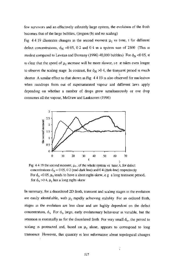
few survivors and an effectively infinitely large system, the evolution of the froth becomes that of the large bubbles, ((region (b) and no scaling)Fig 4 4 19 illustrates changes m the second moment |i2 vs time, t for different defect concentrations, dN =0 05, 0 2 and 0 4 in a system size of 2500 (This is modest compared to Levitan and Domany (1996) 40,000 bubbles) For dN <0 05, it is clear that the speed of \i2 increase will be more slower, i e it takes even longer to observe the scaling stage In contrast, for d^ >0 4, the transient period is much shorter A similar effect to that shown in Fig 4 4 19 is also observed for nucleation when raindrops form out of supersaturated vapour and different laws apply depending on whether a number of drops grow simultaneously or one drop consumes all the vapour, McGraw and Laaksonen (1996)

Fig 4 4 19 the second moment, \x2, of the whole system vs time,‘t, for defect concentrations dN = 0 05, 0 2 (mid-dark line) and 0 4 (dark-lme) respectively For dN <0 05, ^ tends to have a short right-skew, e g a long transient period, for dN >0 4 , 1 2 has a long right-skew

In summary, for a disordered 2D froth, transient and scaling stages in the evolution are easily identifiable, with \i2 rapidly achieving stability For an ordered froth,stages in the evolution are less clear and are highly dependent on the defect concentration, dN For dN large, early evolutionary behaviour is variable, but the situation is essentially as for the disordered froth For very small dN, the period to scaling is protracted and, based on |0,2 alone, appears to correspond to long transience However, this quantity is less informative about topological changes

117

taking place in the system than [i2(n*) This suggests that the period of many, rapid changes is relatively short and that the majority of the system stabilises fairly rapidly The final constant value of (i2 will be obtained only if the initial system isvery large This suggests a critical concentration of defects for finite systems, below which scaling is not observed The concentration of defects also appears to determine the length of the transient period f

118

Chapter 5 MC Simulations and other Considerations

5.1 System Simulation with MC: Introduction

There are clearly practical limitations in extending simulations on cellular networks such as 2D froths by direct methods given the sequential nature of many of the original algorithms and limited hardware The available options thus include parallelization or vectorization of the algorithms and alternative simulation methods, which deal with system statistics as aggregates rather than as detailed topological alternatives One other option would be changes of hardware but this of course calls for massive investment The performance of distributed systems may offer alternatives to super computersWith respect to the development of parallel algorithms, this would seem to offer a better option, although for some of these complex systems, notably the froth networks, such development offers a whole new project in itself, Heermann and Burkitt (1991) Neither is parallelization always appropriate for systems of complex type and also of course generates its own problem, for example load balancing algorithms, Hegarty et al (1996) Nevertheless, in subsequent section of this chapter we discuss some of the implications for a parallel approach The third options of simulations which deal with the statistics of a hypothetical population which in some sense mirrors the real one, is considered first in what follows In particular, if we continue with the example of 2D froth, we note that direct simulation of the evolution of several thousand cells on the system used on VAX in DCU takes of the order of two days (system size = 3000 cells) It appears, therefore, that this approach is limited for systems consisting of large numbers of cells It is also not clear that the direct method will be sufficiently flexible to modify easily for other related cellular systems, e g grain growth, in particular where an increase in scale influences both the effects observed and the time taken for them to stabilise In what follows, we therefore consider alternative simulations of Monte Carlo type for these systems

119

5.1.1 Simple SystemsThe Monte Carlo (MC) approach (introduced Section 2 5) has been used successfully on a number of problems on surface behaviour for simple cellular systems, e g cellular automata (CA) models, spin systems, and percolation models, Hammersley and Handscomb (1964), Binder (1986), Stauffer (1991), (and also Jain (1992)) Long-term large-scale effects for those systems can be investigated in terms of a large number of discrete rather than continuous samples The generation of random numbers is used to determine whether or not an event relating to, for example, an atom or energy change takes place The system is then allowed under certain criteria to move to a new configuration

5.1.2 MC for Froths: General PointsWejchert et al (1986) provided an alternative simulation method for studies of froth evolution Based on discretization of the froth, each bubble is assumed to consist of a cluster of hexagonal cells, (samples), of the same size and shape Early MC studies were used to investigate the effect of the area constraint, X, on time taken to achieve froth equilibriumGiven that froth coarsening involves the loss by a T2 process of n-sided bubbles with n less than six, then disappearance initially involves gradual bubble area shrinkage The mechanism of this MC simulation is thus to model basic hexagonal cells flipping in bubbles which have no of sides n less than six in every MC trial, where each bubble consists of an aggregation of these basic cells As a cell flip is "allowed", so the bubble’s area shrinks till it eventually disappears The MC approach can thus also be used to investigate the influence on froth evolution of bubble area, area difference, neighbouring cells and so onThe total energy of a 2D froth is given by E= 2a dX lv where a is surface tension,(or surface energy), which creates pressure differences These result in gas diffusion and the summation is over all bubble walls, of length, lp i e the boundarylengths of all bubbles To minimise the surface energy of the cells in the network, the total energy Equn (4 2 6) reproduced here for convenience, is given by

120

(1 j) (i'jO bubble k

where cell (i',/) is the nearest neighbour of cell (i,j), so is the length ofbubble side, (i e length, /¿), where 1S surface tension between cell (i,j)and ( i ' , j ' ) So, S g ^ g ^ y ) =0 if cell (i,j) and its neighbour cell (i',j') belong to the same bubble, but otherwise =1 The total No of bubbles = N, Aact and AKir are actual area and target area of bubble k, with Aact determined by Equn (4 1 2), and X, a constant that specifies the strength of the area constraint

5.1.3 Implementation for 2D Froth!

Conventional MC simulation using the Metropolis method involves steps which for a soap froth, may be represented for one MC trial by(I) Start with a Voronoi network of bubbles consisting of hexagons from which a cell is randomly chosen(II) Randomly select a new cell from one of its six nearest-neighbours (m)Calculate change in surface energy AE, Equn(5 1 1)(iv)For AE<0, accept new configuration (Typically AE depends on control parameters,(v) For AE>0, retain the old configuration

We illustrate cell flipping for one MC trial in Fig 5 11, where the following sequence applies If a randomly chosen cell (l, j) of a bubble k l is in the boundary of an nl-sided bubble kl and an n2-sided bubble k2, then randomly select one of six nearest neighbours of cell (i,j) If the new cell, either cell (i+l,j) or (i,j+l), shown in Fig 5 11, satisfies the condition of AE<0, (step(iv)), the cell (i,j) will flip from bubble kl to its neighbour k2, irrespective of whether bubble side No , nl is less than, equal to, or greater than n2 Then the area difference between bubble kl and k2, AA, will update due to the actual area, Aact of bubble k l and k2 having changed, while the target area, Atar of bubble k l and k2 will stay the same

H=(1/2N)ZE5 o (lj)a (l,/ r l + (VN)X (Aact - A J 2 (5 1 1)

121

Fig 5 1 1 An example of Cell flipping in MC simulation

A more complex example is to consider a cell at the boundaries of three bubbles, or more, see Fig 5 1 2 and 5 1 3 If cell (il,jl) occurs at the boundaries of three bubbles k l, k2 and k3, (with notation similar to the two bubble case), then, if any one of the nearest-neighbour cells ((il+ l,jl), (il,jl+ l), or ( il- l,jl+ l)) satisfies the cell flipping condition, AE<0, then cell (il,jl) in bubble k l may flip to either bubble k2 or k3 across the boundary The choice of nearest-neighbour again is random Area difference, AA will update to give, A A j^A A ^+l, and AAk=AAk -1 (k= either k2 or k3), and again, the target area of bubbles, k l, k2, and k3, (Atar (kl, k2, k3)) remain the same

Fig 5 12 Cell flipping between three bubbles

122

Fig 5 1 3 Cell flipping between four or five bubbles

For a T2 process, simulated by MC, energy changes, AE, (cell by cell reduction or flipping), will be negative for small bubble cells However, AE depends on the nearest-neighbour of a given cell chosen, the parameter A. and so on We also need to know the characteristics of recipient bubble, n, <A>, AA The evolution time is measured by Monte Carlo Step (MCS), which refers to the repetition of one MC trial until all cells have been considered5 In initial simulations, we choose the area difference, due to bubble diffusion between actual and target area, AA, to be 5% of the average area of a 5-sided or 7-sided bubble, 1 e AA=-(n-6)*5%*<A0>, where AA=Aact-Atar, <A0> is the initial average area of bubble in the system Thus, AA=0 for a six-sided bubble, AA>0 for a n-sided (less than six) bubble, and AA<0 for a n-sided (greater than six) bubble Froth equilibrium is achieved for the total average area difference less than the given maximum difference

123

5.1.4 Froth Coarsening

5.1.4.1 Notes by MC

(i) CPU time is affected by A,, but also by value of control parameter, (temperature equivalent, T=0 always for step (i) to (v) in a single trial) Also affected most importantly by A A,

(u) No of sides, n, of a nearest-neighbour bubble will change with a bubble disappearance (Euler’s law) Thus, A ^ , AA for nearest-neighbours of a disappearing bubble must be updated instantaneously before next MC trial

In what follows, we consider the importance of the choices of X, AA, <A> for an efficient and realistic MC simulation following Wejchert et al (1996)From the procedure described it seems clear that achievement of a “scaling-state” should depend on the environment of a disappearing bubble, (i e large or small neighbour), and therefore on percentage reduction in target area, Atar, AA asmight be expected, (e g 2% average area will cause less cell flipping in one MCS, whereas large neighbours make cell flipping more likely, since energy difference, AE, condition more likely to be satisfied) and so onHowever, the final disappearance of a "bubble" may be slow since the last cell can take a long time to flip When a cell is the only cell in a 3-sided-,bubble, it must flip to nearest-neighbours, possibly taking many MC trials because it is a stochastic procession) This final disappearance also implies a reduction in the No of sides n of bubbles k2, k3, and k4 Both Aact and Atar for k2, k3 and k4 will updateinstantaneously, and hence area difference, AA will change to AA', where AA'= - (n-6)*5%*<Al>, given our choice of area difference above This applies equally for a 4-sided or a 5-sided bubble So, for any n-sided (n<6) bubble, when the last cell in the bubble flips to one of its nearest-neighbours, bubble disappearance will occur accompanied by the reduction of the number of sides in nearest-neighbour

As a further series o f points on the MC simulation, we note the following

124

bubbles This leads to the typical fluctuations in fj,2 m froth coarsening, which we have noted earlier, Section 4 2

The mam structure by MC method is given as follows, (for further details see Appendix E)

// Froth Program by MC Method//CALL input // input dataCALL setup // Initial Configuration (Voronoi network) CALL Eguil // Equilibrium do 10 i=l,nCALL Diffus // diffusionCALL Equil // Equilibrium implemented by MC trialsi = i + lCALL OUTPUT

10 continueCALL OUTPUT END

SUBROUTINE Cflip //MC trialItime= Itime +1 //time stepOcell=ga(î,j) // a cell (i,d)iel=iel+l // calculate the first term of

initial energy of a cell N e w k = m t (ran ( 1 ) *6)+1 //random choose one of the six

neighbours of cell(1 ,3 ) ie2=lambda(dvl*2+dv2 *2 )//calculate the second term

of initial energy fel=fel+l // supposed a cell is flipped,

calculate its first term of energy fe2=lambda(dv3*2+dv4*2) //calculate its second term

of energyoldenergy=iel+ie2 //the sum of energy before flipping newenergy=fel+fe2 //the sum of energy after flipping

if (newenergy.le. oldenergy)then //energy difference greater than 0 ,)

make= true. // accept the new configuration else // Continue MC trial if temperature>0

125

if(temp.g t .0)thenif(exp(-(newenergy-oldenergy)/temp) gt r a n (1))thenmake= trueendifendif *1,

endifEND

5.1.4.2 Performance under Different Choices fo r <A> and XFrom the mechanism described in the last Section, it seems that whether a cell (i,j) flips or not may be dependent on the initial environment We have implemented froth evolution with two different Voronoi networks for a 2D froth of size 1600 bubbles with 400* 400 cells Here we measure the evolution time in terms of a Monte Carlo Step (MCS), which is defined as previously, (Section 5 1 3), l e the repetition of the sequence for one MC trial until all cells in the system have been consideredIn Fig 5 1 4-5, we show variation of CPU time on MCS with the effect of refining A. and choice of area difference, AA In Fig 5 1 4, we show the effect of varying the choice of area difference AA (2% and 5% respectively) on the second moment,H-2 time (measured in MCS’s) In Fig 5 15, the effect on CPU tune (again in MCS’s) vs A. is shown where the interest is in refining A, to produce greater response for reasonable time taken For any value of A, much beyond 0 4, however, CPU time escalates rapidly, in agreement with the similar result obtained by Wejchert et al (1986) The CPU time is clearly longer due to slow energy change for large values of parameter X, Equn (5 1 1), Fixing the area difference as 2% of mean area <A> (Section 4 13) leads to a smooth evolution of |12 vs time This is not surprising since ]Xj is sensitive to bubble disappearance at the lower percentage, thus it is less difficult to get flipping, and changes are less drastic Results for quantities of interest are in good agreement with those obtained by previous simulation methods

126

time (MCS)

Fig 5 1 4 the second moment changes vs time (MCS)

100 -

_ 80 - tnoS. 60 0 E= 40 +

20 -

0 -I----- 1----- 1----- 1----- 1----- 1----- 1----- h0 01 0 2 0 3 0 4 0 5 0 6 0 7 01

Fig 5 15 Time (MCS) taken vs X

51.4.3 Performance of Bubble AreaThe initial bubble area A also appears to influence bubble disappearance Consider, e g a three-sided bubble with different n-sided nearest- neighbours, (n= 4, 5, 6, 7) For a small value of X, it is clear that the energy difference for all n-sided bubbles satisfies the condition AE <0, while for large X, AE will vary with different no bubble sides, e g for n=6,7, AE<0, for n<6, AE >0 The actual value of E depends, of course, on the Equn (5 11)In particular, we are interested here in the influence of bubble area on bubble disappearance We consider the influence of initial area distribution for two types of Voronoi network, (l) no hard disk version, where the initial area distribution is non-uniform, or polydisperse, with (J.2 = 1 87 (u) hard-disk modification, where

127

the initial area distribution is not the same as (1), but still poly disperse, with |i2 = 1 09, (111) hard-disk, where the initial area distribution is different, roughly

i,uniform, or monodisperse, with 112 =0 97, closer to (11)For different Voronoi setups considered, the evolutionary behaviour for both polydisperse froths, initial conditions (l) and (n), is similar, and indicates a rapid decrease in the No of bubbles with time, which is more marked for the froth with higher initial disorder or less uniformity of bubble area However, for roughly uniform area, initial condition (in), the decrease in the No of bubbles with time is much slower, although long-term behaviour is again similar to the previous cases ((i) and (n)) We show the change in the No of bubbles disappearing with time in Fig 5 1 6

time (MCS)

Fig 5 1 6 No of bubbles vs time

In previous experimental work, Glazier et al (1987) also note that the apparent rate of shrinkage of bubbles with few sides is smaller than that predicted by a pure linear fit If Von Neumann’s law holds m unmodified form, the evolutionary behaviour of froth with initial conditions, as for (n) and (m), l e roughly the same side distribution, but totally different area distributions, should be the same However, we find that there are differences at the early transient stage, implying that initial bubble areas influence the rate or nature of froth evolution This might be taken to suggest that a modified form of Von Neumann’s law by Icaza-Herrera and Castano (1995), which accounts for area distribution, should apply to the early evolution. A possible form has been conjectured to be:

128I

dA/dt= kAa (n-6) (5 1 2)where k and a (0< a< l)are constants, a=0 when Von Neumann’s law holds in unmodified form, and a = l for a normal froth, Icaza-Herrera and Castano (1995) From Equn (4 4 1), for the uniform area case, dA/dt ~ (n-6) applies A modified law for different area distributions also gains some support, however, from e g Herdtle and Aref (1992), who demonstrated some anomalous evolution results for bubble disappearance Such anomalies appear, however, to relate to the early stage of evolution and Von Neumann's law is appropriate for the evolution as a whole In contrast to direct simulation, the MC method is able to model large system size for less CPU time, (even though here only give an example of system size of 1600 bubbles) Moreover, the direct simulation program is much more complex and less flexible than MC methods MC has been used to study other network pattern problem, e g gram growth, Anderson et al (1989) However, the disadvantage by MC is also obvious, e g the detailed information of evolution procedure obtained by the direct method is not available to anything like the same extent although MC results are fully acceptable on an average basis

5.1.4.4 Summary• i

In summary, considerable effect on the froth evolution is obtamed by varying the control parameters of a MC simulation of 2D froth In particular, the construction appears to emphasise the importance of the environment on the flipping of a component cell of an n-sided bubble (n<6) and hence on that bubbles disappearance In particular, we consider the important of the environment on the flipping of a component cell for a bubble with n<6 and hence on that bubble’s eventual disappearance It is obvious that a large target area, AUir and areadifference, AA, in this context implies that the scaling state is achieved more rapidly during froth coarsening Additionally, A modified Von Neumann’s law best appears to after an alternative explanation of the influence on early transient effect of area

129

5.1.5 Technical Implications of Froth5.1.5.1 Theoretical Implication

A realistic froth must include 3D and a few attempts to address the 3D case have been made so far Clearly, such a cellular network is both more challenging and complicated and thus, is very difficult to describe using a direct model as in 2D Of the approaches tried for a froth to date, Frost et al (1988) used a discrete description of the structural elements themselves, while Nagai et al (1990), considered only vertex points joined by straight lines as in the,topological model, (Section 4 2 3 3) Other aspects of the problem have been considered, e g by Weaire and Glazier (1993) who give a relation between volume and number of faces in coarsening cellular patterns, and by Weaire and Phelan (1994) who have obtained a more efficient space-filling structure of 3-D froth which challenges Kelvin’s original structure More recently a logistic map formulation has been considered by Aste and Rivier (1996) For a recent review, see Weaire and Phelan (1996)It is instructive to consider some of the reasons why a three-dimensional cellular network is so much harder to simulate than its two-dimensional counterpart, despite the fact that we can theoretically define very many dimensions in computational terms The factor of computer time is crucial for simulation in 3D, because although the fraction of the volume affected by edge effects is much larger than in 2D, the time taken for equilibration to take place makes the simulation of large systems prohibitive The memory storage and computation time required for such simulations is huge, limiting severely the size of system that can be simulated, and therefore making it difficult to obtain reliable information about scaling states which apply in the asymptotic limitIn addition to these common technical difficulties the simulation of our specific cellular network, namely the realistic 3D froth present some additional problems, which are intrinsic to the nature of the problem These include the fact that distribution functions which are fundamental to the statistics are more difficult to obtain since not all the structural details can be accessed simultaneously and with

130

ease Furthermore, the theory of the 3D froth faces an even more serious obstacle in that the basic equations for 2D froths, (e g Von Neumann’s law, Euler’s rule), both fail in three dimensions Polygonal cells in 2D are separated by circular arcs with constant mean curvature that meet at equal angles of 120° In contrast, polyhedral cells in 3D are separated by minimal surfaces with uniform mean curvature, three faces meet at equal dihedral angles along each cell edge, and four edges meet at each cell vertex at equal tetrahedral angles of cos 4 (-l/3) =109 47°In fact, the average number of faces, <f> of bubbles in a three dimensional froth can vary considerably, though most experiments yield a value near f=14 Instead the relation given by Nagai et al (1990) is

<n>=6 - 12/<f> (5 1 3)

This implies that two parameters (i e n and f) are needed to characterise a cell in a three dimensional cellular structure as opposed to one (=n) in 2D In the case of n=5, f=12, corresponds to the pentagonal dodecahedron, which is an important structureThe elementary topological transformations also occur in rather different ways compared with 2D A T1 process whereby the vertices common to an edge coalesce creating a new side, and a T2 process by which cells disappear directly by shrinking are shown in Fig 5 1 7(a) (b). It is still not known however, how many different types of T2 processes there are because the average surface curvature of a bubble with tetrahedral angles 109 5° is not determined solely by its number of sides

131

(a)

(b)Fig 5 17 Elementary topological transformations m 3D

(a) T1 process or switching, (b) T2 process

The minimum information needed to determine the growth rate is also not known Rivier(1982) has suggested “patching up” with the relation

dAf /dt = k(< f> - / ) (5 14)where f is the number of faces of the bubble or gram, Ay its volume, and <f> is the mean for all grams This equation is reminiscent m form to Von Neumann’s law, but there are subtle differences between them Equn(5 1 4) describes the evolution of an ensemble of cells instead of that of an individual cell Furthermore it cannot be integrated to obtam the dependence of A j on time The topological networkmodels in 3D, such as Equn(5 1 4), would appear to be no more difficult to handle than those m 2D, but there are ten or more types of disappearing bubbles Recently, Rivier(1985) derived a three-dimensional version of,(the Aboav-Weaire law

mj{n)=c+l/n [f(5 -c )+ (c -ll) ] (5 1 5)

132

where mf(n) is the average number of sides of the neighbouring faces of an n-sided face belonging to an f-faceted cell, and c is a constant Computational verification of this result is still lackingDurian et al(1990) performed a systematic experimental study of coarsening in three-dimensional foams By monitoring the optical transmission of shaving cream foam over time, they found that the average bubble size in the bulk increases as apower law tP with (3 = 0 47± 0 05 Observations of foamj surface by optical microscopy showed that the dynamic processes consist of structural rearrangements of bubbles which differ from T1 processes in both nature and timescale These rearrangement events are possibly due to the high liquid content of the foams used in the experiment In fact, the examination of the microscope pictures shows nearly spherical bubbles The origin, scaling behaviour and effects of these rearrangements upon the coarsening were not studied Computationally the question of computing capability and power available is closely linked to these difficulties of pinning down the underlying mechanisms and structures Some successes have been recorded For example, the Potts model can be extended to three dimensions provided that sufficient computer time is available Anderson et al (1989) have run simulations on a 100*100*100 lattice For lattices with different anisotropy, these authors made a variety of distribution function measurements, obtaining <f> =12 9 The agreement' with experimental values for metal grains is good, with the residual discrepancy compatible with anisotropy effectsGlazier (1993) indicated that the coarsening behaviour of the 3D Potts model depends on grain topology, and concluded that a similar but weaker law holds for ensembles of bubbles in 3D An expression corresponding to that found by Durian et al (1990) for shaving foam (section 5 1 4), was given by Glazier to be

V-i/3 dV/dt = k(f-f0) (5 1 6)where k is a diffusion constant, f is the number of faces of a gram, f0 is a constant, and V is the volume of a gram havmg f faces Equn(5 1 6) shows that the average canonical growth rate of a gram depends linearly on its number of faces and is dependent on its volume, which is analogous to the modified Von Neumann’s law

133

of Icaza-Herrera and Castano, which we have given in Equn(4 1 2) However, those equations only hold, of course, on average The growth rate of any individual grams need not depend on its number of faces, for example, some 16- faced grams grow, while others shrink Sire (1993) has also addressed the reason why only an average growth law holds m 3D Glazier has postulated a corrected average value for <f> based on this work with f0=15 8, and subsequently found to obey an expression

f0=<f> (l+ |i2/<f>2) (5 1 7)(Weaire and Glazier (1993)), with <f> the average no of faces Further Potts model simulation results gave <f>=13 7 and f0=15 8 ±0 4, m agreement with theresult of Glazier (1993) The evidence then supports the view that the averaged growth rate in the Potts model is a linear function of the number of faces Equn (5 1 7) will apply to any other coarsening system, which has similar connections between growth rate v and f The accumulating evidence therefore continued to favour the use of statistical of simulation methods to further explore 3D froth features

5.1.5.2 Technical Implications for Froth by MC MethodThe optimal structure for a monodisperse foam has been a subject of mterest for centuries The question is what spacmg filling arrangement of cells of equal volume has minimum surface area Kelvm (1887) proposed a truncated octahedron as a likely candidate for the optimal arrangement Weaire (1994) suggested two cathedral structures as a natural choice for mtermediate values of liquid content These occur m the chemistry of tetrahedrally-bonded materials and there is a close analogy between tetrahedral structures and the froth or foam problem In a recent breakthrough, Weaire and Phelan (1994) have given a counter-example to that of Kelvm which has a significantly lower surface energy The method used the surface Evolver software, (developed by Brakke (1992) (1995)), to minimise surface area, subject to the constramt of fixed cell volumes, for successively finer tessellations of the ongmal cell faces In this way, the curvature of the surface can be progressively approximated with mcreasmg accuracy It is found that the final Weaire-Phelan

134

structure, consisting of six fourteen-sided polyhedra and two liTegular pentagonal dodecahedra, has surface energy which is approximately 0 3% less than that of Kelvin’s solutionWeaire and Glazier (1994) also developed a simple construction based on the Kelvin and the Williams partitions that generates periodic or quasipenodic 3D partitions It has been used to distinguish the mmimal-area structure under conditions of equal volume and equal pressureGiven that the precise relationship between the topology and the rate of growth of a bubble for the 3D froth is not well-understood, most algorithms developed so far have concentrated on the whole structure level rather than the level of an individual bubble However, MC simulation appeared to offer reasonable possibilities of extension to the 3D case since dealing with an ensemble of cells is an intrinsic mechanism of the approachParalleling the 2D froth method, we considered the discretization of bubble volume by a cluster of samples (units) Given that the number of a given bubble’s faces and that of its neighbours are more complex than for 2D, we consider initially a simple basic structure 1 e the cubic cell, so that aggregates of cubes would form the network bubbles Implementation of cell flipping in cubic structure is a generalisation of the 2D case, but allocation of a flipped cell to nearest-neighbour bubbles is much more complicated Clearly, a bubble’s disappearance again depends on whether all constituent cells have flipped to one or more nearest- neighbour bubblesSince the energy of the 3D system is related to the bubble’s surface energy, 1 e the length of boundaries or of all bubbles’ face, a cell-flipping will affect either one or the other The energy would be expected to have an equation which crudely parallels that for 2D, given e g by

H=(1/2N)££S + (X/N)Z (V ,a - V urP (5 ! 8)

( i j J c ) ( i ' j ' J O b u b b l e k

Here, the analogy to the basic unit of the hexagonal cell in the 2D case is now a cubic cell, (i',j’,k') is one of the nearest-neighbours of cell (i,j,k) and summation is over all faces The maximum no of choices for bubble assignment in cell-flipping is

135

now 7, as opposed to 5 in 2D; clearly a single MCS will include more complex MC trials.For a 3D Voronoi network configuration, Equn (5.1.6) could be used as the approximate equivalent of Von Neumann’s law in the 2D case. Assuming the volume difference due to bubble diffusion between actual volume and target volume, AV, to be 5% of the average volume of all bubbles, and the average No. of faces, <f> equal to 14, we can implement a cell flipping by MC method on 3D froth. Similar to 2-D froth, assumed for a 14-faced bubble, AV =0, for an n-faced bubble, (n<14), AV >0, for n>14, AV <0. Choosing the same volume difference for all the non-14-faced bubbles will obviously, however, introduce a bias in the 3D froth evolution.

5.2 Other Techniques

Both cellular automata and molecular dynamics techniques have also been used to study some cellular network models, in particular, grain growth and solid foam.

5.2.1 CA for Grain GrowthGrain growth, as an example of a cellular structure, is of great interest since it is one of the most important features in the control of micro structure. The energy of grain boundaries at equilibrium and topological requirements are two important factors in modelling grain growth, Atkinson (1988). Theoretical, experimental and simulation models have all been used to investigate system properties and in particular, the MC method has been successfully used to solve this problem Based on the transition probability, MC methods have been applied to simulate processes of recrystallization, normal grain growth and abnormal grain growth, (Srolovitz et al. (1984), Anderson et al. (1989)). For a recent review, see Weaire and McMurry (1996).Similarly to the froth, grain growth is one of the natural structure-evolving processes. Since the grain boundary network has similar patterns and characteristics to those of biological cells and ecological territories, cellular automata (CA) would seem to be applicable to their study. Hesselbarth and Gobel (1991) first applied a

136

CA model in primary recrystallization simulations and Liu et al (1996) further developed a formal CA model with further assumptions for the grain growth problemUsing Von Neumann’s definition of neighbourhood for a CA model, Wolfram (1984), Liu et al (1996) have given the transition process as

x(i,],t)= F[x(i,j,t),x(i,j+l,t),x(i+l,j,t),x(i-l,j,t),x(i,j-l,t)]' (5 2 1)where x(i,j,t) represents the states of (i,j) cell at time t The function F is the transition rule, which can be defined in a various way The dynamics of CA are governed by local rules, (as we have described in Section 2 3), so that the locality of the dynamical rules allows efficient and flexible treatment of complex geometries Thus, whether the final state of the system after a given period of time is homogeneous, chaotic or complex, depends on the definition of the transition rule The Game of Life is a well-known example exhibiting variety and complexity in the development of CA even for simple rules, Vichmac (1986), but much more complexity is possibleLiu et al (1996), for example, have modified the transition rule Equn(5 2 1) to implement gram boundary migration due to curvature effect A gram boundary isassociated with a positive surface energy and migrates m some way to lower

ienergy, e g two cells with different states are separated by a minimum unit length of gram boundary The results of Liu et al (1996) on gram size distribution and growth kinetics are m agreement with those obtained from theory, experiment and MC simulationIn general, the basic difference between the Monte Carlo (MC) method and CA lays m the transition between states of a cell m the system In the MC method, the state transition is realised by randomly taking a number m the state of N=1 to Q, then puttmg it m the cell which is ready to change, calculating the energy difference, AE, between the old and new configuration and giving the probability of transition For AE<0, a new configuration is accepted, with the probability P=l, for AE >0, with P = exp(-AE/kT) Usually, the probability, P, is different from cell to cell m the MC simulation model In contrast, for a CA model, the new state of a

137

cell comes from its neighbour cells, so for every cell, there is constant energy barrier, which must be overcome in a state transition with the same probability

5.2.2 Molecular Dynamics on Wet FoamDurian (1995) discussed wet foam by focusing on entire bubbles rather than vertices, and proposed a simulation model, which has been constructed for the molecular dynamics approach (Section 2 5) In terms of structure and dynamics at the bubble scale, the model has been shown to reproduce the hall mark behaviour This approach also allows reliable study of formations and flows at length scales greater than the average bubble size However, the weakness of this method is that it can only be used in wet foam, not dry foams since no degrees of freedom are introduced for the bubbles shapes Gardiner et al (1997) also used molecular dynamics to analyse the scaling behaviour of 3D solid foam

5.3 Computer Simulation Implementation

5.3.1 Simulation ApproachesEvolutionary dynamical systems have attracted considerable attention in recent years Many efforts have been made to investigate their properties Computational modelling techniques have provided new and valuable insight into the studies of these complex systems, both in terms of testing microscopic theories as well as practical methods for modelling processes as a whole Although some current programs are less sophisticated than those of commercial software, a wide variety of techniques and computational environments have been used Our aim has been to investigate several simulation approaches as a means of examining the dynamical behaviour in complex systemsTraditional modelling and simulation has tended to concentrate on mathematical representations of complex physical and other systems with strong reliance on both numerical modelling and discrete methods For more complex systems, there are two strategies available One is to improve theory at higher levels which usually means improving on an approximate form and another is to simulate the behaviour of mam elements Theory thus tries to resolve computational difficulty by reducmg

138

detailed information to a few degrees of freedom For example, the objective of statistical mechanics is to observe not only the underlying state itself, but also the probability of the system being in any particular stateIt appears that indirect simulations, e g MD, MC are less information rich than direct simulation (e g froth example) It is obvious that direct simulation can specifically provide us with more detailed information during the evolution on hundreds or, better, thousands of cells However, it is far from ideal to try to obtain a scaling index from simulations limited by time and scale, so that improvements in the algorithms and their efficiency are clearly needed for fixed hardware provision In contrast, the MC approach appears to offer the better general method for proceeding on a variety of associated questions e g gram growth and other similar networks

5.3.2 Languages Requirement i,<3-

Currently, the most popular languages for computational scientists are Fortran 77, (Fortran 90), C and C++ Fortran, through the most popular for many years, however, does not allow the programmer to structure programs so that they reflect the logical order of idea mvolved m addressing a problem, and it is often complicated to delineate new contributions and modifications to existing large scientific Fortran codes Due to inflexibility, Fortran appears to be losmg ground, although Fortran 77 is much easier to use than C and C++, which is growmg m popularity From a computer science pomt of view, there is little difference between C and Fortran, except that C has marginally better facilities for structuring programs than the ongmal Fortran 77 Far more differences exist between the various styles of parallel programming, where these differences are already havmga big impact on software development for computational science and makes

rmcreased familiarity inevitable fFrequently, because of the longer development time of the language, Fortran compilers are more robust and efficient for scientific applications m particularly for supercomputers, although special version of C may perform as well or better on some massively parallel machines Graphics and visualization are almost entirely done in C/C++ although FORTRAN implementations are possible It is also

139

possible to use Fortran subprograms in C/C++ codes For scientific programmes, we can take advantages of both languages, e g keeping theA numerical Fortran routines for difficult number crunching and designing the software package with an object oriented language In recent years, some of the more popular commercial numerical routine libraries have also been released in C version Computer languages keep evolving rapidly, and it is possible to discern a trend toward formal languages A wide array of routines accomplishes a range of tasks from elementary to very complicated For most users, programming will be limited to the connection of such routines by using graphical or verbal syntax More recently, visualization packages in physical and other scientific applications have enjoyed a tremendous surge of interest For instance, Surface Evolver has now become the standard software for computing the geometry of foams, Kraymk and Reunelt (1996)

5.3.3 Algorithms LimitationIt is known that the application of algorithms to the behaviour of very large systems would not have been possible, without highly optimised programs that reduce the memory requirements and the execution time Even with the current, relatively advanced technology and sophisticated algorithms, most simulations are limited to a relatively small range of scales They are prone to various types of error, and require a long time to implement Choosing simplified mathematical models is an accepted option to understand and solve the various computational problems with a view to improving the system representation Much work here has been concerned with two-dimensional simulations and experiments as a simplification of naturally occurring systems Each approach considered, however, has its limitations For example, in the 3D froth model, the main difficulties of the MC method he in the fact that the number of possible configurations of each bubble becomes enormous with a large number of degrees of freedom which must be simultaneously handled System size limitation could be another problem for all simulation approaches Further developments for both software and advanced hardware resources are required Coding methods such as multi-spin coding can normally be extended to the three-dimension problems and

140

also apply for the froth case. However, the large number of variables, and operations might not provide easy implementation and the memory is another factor.

5.3.4 Limitation of Simulation MethodsSimulations themselves are not necessarily reliable since they also generate different errors intrinsic to the simulation method. For example, statistical errors occur in drawing a finite number of partially correlated samples, numerical errors occur in the algorithms, and round-off errors arise from finite-size effects. In spite of this, the simulated behaviour of the model gives an approximate analogy of a system’s actual behaviour. The real difficulty lies in determining the level of error, aggregated from those various causes and the degree to which it affects the realism and accuracy of the system representation. There is, of course, no single answer to this question and for the majority of simulation work, there is a need to perform may trials and repetitions of the same experiment to test the limits of the simulation and observe carefully end effects. Also, of course, to test vs. known results as a control on the simulation veracity.Considerable effort has been spent in the development of computational problemsolving environments for physical and related systems. Some attempts have been made to integrate various software components into a unified system hiding the underlying complexity from the user. This is an "idealised" improvement, with the goal of solving all aspects of a problem including simulation, data analysis and visulaization. Unfortunately, such systems tend to provide very poor performance on large problems even if performance is reasonable for commercial applications. Consequently, they are generally unsuitable for scientific computation.However, the idea of providing integration of simulation and data analysis is an interesting one. The approach must clearly emphasise transparency rather than attempting to create a highly sophisticated package with over-elaborate interfacing. In short, tools should be simple to use, offer high performance, be maintainable across a wide variety of machines rather than get in the way of research on a limited subject. In particular, the following features are needed to measure the development of simulation software in scientific applications.

141

• Performance and memory efficiency• Extensibility• Support of existing code

More advanced developments include controlling applications with scriptinglanguage, rather than relying solely on compiled languages, such as C or Fortran

' ‘i *The use of interpreted scripting language for dealing and interacting with physicsapplication has been the subject of recent exploratory work by computationalscience researchers The idea is quite simple, providing a high-level interface, suchas Matlab Using this package, users can control physics and other applicationsinteractively by entering commands, writing receipts and adding additional functionlists in the interface language, without having to modify the underlying code Thesoftware package, the Surface Evolver, is one such package which is applicable toa variety of practical problems and has been mentioned earlier in relation to 3Dfroth work

142

6.1 Introduction

Nature provides many examples of systems which have an essentially single or network cellular structure The statistical properties of their long-term behaviour can be investigated by e g monitoring the occurrence of specific "events" or network evolution through time Insight on changes ranging from the minor to the catastrophic can be gained through computational modelsThe goal of scientific investigation is to understand how nature works Originally, two options were available to do this, namely experiment and theory The traditional approach consisted of modelling system equations directly and then solving these equations, either manually or by computer routines Unfortunately, this breaks down where analytical solutions are not available* or where technical difficulties prohibit numerical solution or when the system being studied is not theoretically well understoodAlgorithms or computer programs, which directly model the phenomena under investigation have increased in popularity This thesis presents a general overview of simulation methods for studies of complex physical and related systems which are of current interest Most importantly, it provides a description and application of some fast and efficient simulation modelling techniques and their potential for further development, together with our implementation of and results on a selection of these cellular system models

6.2 Techniques Implementation

We have implemented several different computer simulation techniques in this work, including direct methods, cellular automata, Monte' Carlo, and have introduced others, such as molecular dynamics, which have not been explicitly used for the work presented here These provide an overview of current popular methods used in investigating scientific computing problems Generally speaking, a number of different techniques may be applied to a given problem, but the choice depends on the aspect of interest In the direct modelling of the 2D froth in 4, for

Chapter 6 Conclusions and Comments

143

example, interest focused on the detailed structural changes, as well as on the long-term behaviour, particularly when following the influence of defects Thus direct simulation methods, for initial studies anyway, provide an obvious choice However specifying a certain system so precisely incurs penalties, in terms of adaptability of the code, together with limitation on the size of the system which can be simulated, when so much detail is being retained Consequently, adaptation to other complex systems which share common features, requires additional effort, even though this may well be considered worthwhile A close analogy to the soap froth, for example, is provided by the metallic grain growth problem, Weaire and McMurry (1996), yet there are distinct differences, notably in the shape of the gram boundaries, which can be far from the ideal minimal surfaces found m the soap froth, and also m the inherent lattice anisotropy This latter feature is of particular mterest, smce it influences the rate of transition between order and disorder, which is much slower than for the corresponding froth, Holm et al(1991) and refs thereinFar less rigidity of codmg is evmced for applications which 'can be reduced to

‘i tmteractions between fundamental and similar elements, where each of these can be m one of a finite number of states For this type of system, the cellular automata approach is a natural choice Its flexibility is reflected m the wide range of problems which CA have been used to model Here we have considered a CA approach to the modelling of dissipative systems, represented by loss of sand grams mduced by perturbation of a quiescent sandpile The sandpile automaton here serves as a model for transport phenomena m general CA methods may be used to directly model the behaviour of the elements or indirectly to approximate them, e g as m immunological CA, Stauffer and Pandey (1992)Features of the CA codmg mclude its simplicity and massive iteration The dynamics of a model typically mclude very few relations, with traditional parallel updatmg Additions and multiplication can be represented by arithmetic additions and multiplications with manipulation at bit level, allowing more efficient code to be provided Examples are given m Appendix B of multi-bit (multi-spin) operation and this has been implemented for the dissipative sandpiles discussed in Chapter 3 and program Appendix E This represents a "cheap" method of incorporating

144

parallelism into the implementation but is obviously inadequate for very large and very complex systems Practical limitations on the use of multi-spin coding do not extend beyond its use for fluid hydrodynamics, although surprisingly good results have been achieved for lattice gas simulation, e g Wolf-Gladrow and Vogeler(1992) Unfortunately, massively parallel computers are not generally accessible, so that most researchers have to make do with general purpose computers with only

1 vone or at most a few processors It is worth noting that’; multi-spin coding (instruction-level) is the lowest of four levels of parallelism, according to Kohring (1991) Others include statement level or chaining, loop level (or strip mining) and process level, where this last separates SIMD and MIMD machines and is a feature of many molecular dynamics simulations Even at multi-spin level, choice of language and availability of machines limits performance and we have briefly discussed these factors in Chapter 3 Performance tests for lattice gas automata in two or three-dimensions, coded in FORTRAN and C with reference to bit operations and integer arithmetic are also reported upon by Wolf-Gladraw and Vogeler (1992)Clearly, sandpile models, such as those considered here, are of interest, not only in their own right, but in terms of understanding other complex systems with many degrees of freedom. Sandpile automata have proved surprisingly successful in the

4investigation of intrinsically puzzling phenomenon, such as SOC MC methodology provides a level of further abstraction when compared to CA modelling and is a stochastic method which relies on good statistical measurements Thus, any problem related to the probability of an event occurring can be investigated through MC in theory Unfortunately, the abstraction of the fundamental problem is not always straightforward, since the more complex the system, the more information is required for accurate statistics Thus, knowledge of Hamiltonian components is very important in terms of successful simulation, since otherwise systematic errors rapidly become very large This is illustrated in the froth case, Chapter 5, where for 2D froth, simulations are fairly successful, whereas for the 3D case, choice of parameter values and level of approximations used, crucially affect simulation performance. One way to overcome these difficulties is clearly to perform an extensive sensitivity analysis across a range of

145

parameters and parameter values, with a view to estimating the amount of variability and bias Some recent 3D froth work, Weaire and Phelan (1996), provides guidelines on which such an analysis might be based In general, the algorithm which we have used involves a more complex Hamiltonian than that used for example by Glazier et al (1990) for the Potts model variant Nevertheless, Potts model simulations which correspond closely to the gram growth problem (see previously this section), have proved successful and suggest that a sensitivity analysis such as that proposed should provide further msight on the importance of the volume component of the Harmtoman in Equn(5 1 8)With the mcreasmg availability of high speed general-purpose computers, many formerly prohibitively complex problems have become tractable by simulation techniques However, even fast programs running for many hours still do not yield satisfactory results m all respects for problems m complex systems, due to practical limitations of time and number of events to be simulated So simulation techniques are inevitably limited at some stage by computer hardware and software The choice of different language and compiler during simulation may be particularly important

6.3 Cellular systems and Phenomena Exhibited ,?fe

6.3.1 SOC and Simple SystemsIt is known that laws governing the evolution of "universes" are often similar and simple Nevertheless, behaviour observed can be highly diverse and several new concepts have been proposed to explam and explore these phenomena, such as chaos, SOC and complexityA SOC system is a class of nonequihbnum system which seem to be capable of generatmg complexity of its own accord Cellular automata as a computational paradigm m computational sandpiles, (described m Chapter 3), have been used to demonstrate self-organised cnticahty, (SOC) The nature of the constramts, either global or local has been considered for various model dynamics Many natural phenomena exhibit SOC, mcludmg earthquakes, fractals, extmction events m biological evolution, landscape formation and so on The characterisation of spatio-

146

temporal processes in general, has received considerable impetus from the investigation of these simple cellular systems, first introduced by Bak et al (1987) In particular, early interest focused on providing an explanation for 1/f noise, through the establishment of scaling lawsDifferent dynamical rules, reflecting deterministic or stochastic perturbation, on both continuous and discrete systems, have been used to demonstrate the existence of SOC in CA and CML models Several universality classes have been shown to exist Models with different dynamics have been found in our work to exhibit SOC for both local and global conservation laws in continuous CML models, whereas SOC is not observed if the conservation law is violated locally in CA models While investigations are limited, they provide a basis for further work, both in stochastic systems and on deterministic systems where the nature of the dissipation is dependent on the local environment and/or choice of loss function While SOC is widely prevalent, it may not provide a universal picture

6.3.2 Cellular NetworksCellular patterns, such as froth and foams, are similar in many biological systems, although the underlying dynamics of the pattern formation is completely different Soap froths are of interest because they are considered to evolve by a similar mechanism to that which governs gram growth m metals and other materials (see previous section) It is reasonable to assume that the essential mechanism of this evolution, (intercellular diffusion resultmg m a reduction of surface energy), governs the behaviour of the soap froth without any significant additional factors It therefore offers us an ideal model system, the study of which provide fundamental insight to the theory of network evolution A typical bubble growth process begms with a nearly ordered configuration and gradually evolves mto a completely disordered pattern with time-invariant topological distributions The studies of froth, m particular, provide an elegant illustration of the evolutionary behaviour of a cellular network Much of the work presented here has concentrated on the problem of the 2D soap froth, where mterest has focused m particular on numerical studies of the froth structure and evolution under various levels of order/disorder or defect concentration

147

Direct simulation methods have proved particularly valuable in terms of obtaining detailed information on changes in the network, although are inevitably limited as to size of system studied Results on abstraction of the problem, or modelling it indirectly via MC methods have been mixed In the 2D case, the network information obtained has been useful although system sizes have not been sensibly extended In 3D, results have been disappointing In part, this is due to the level of detail retained and in part due to a weaker theoretical background for 3D networks in general Nevertheless, a prototypical implementation has been achieved, (see programmes, Appendix E), and provides some basis for extension to other network systems, such as the metallic gram growth problem, e g Holm et al (1991)

6.3.3 Common Features

We have discussed properties of two different types of cellular-structure models From the analysis and detailed discussions, it is clear that these systems share some common characteristics Both are e g non-equihbnum systems, which evolve accordmg to mternal or external forces Nevertheless, distinctive differences exist, not least m the level of interaction considered, and consequently, give rise to diverse behaviour Much of the work here has been concerned with dissipative effects and their influence on the evolution of these many-cell systems havmg different spatial dependence It is conjectured that a dissipative system keeps its structure at the expense of energy flowing, either from the local dynamics rule, or from the open boundary, or both Further, the new structure can possess either coherent or chaotic behaviour 1 e m the long-term, distinctive asymptotic behaviour must occur One obvious and immediate question arising from the work

1so far is thus whether SOC can occur m cellular networks7 Some early studies on froth rheology have conjectured the existence of SOC on avalanching m froth under stress, Hutzler et al (1995)Other network models apart from soap froth, also appear to exhibit SOC For example, considermg domain wall motion m disordered ferromagnets driven by an external field, Bak and Flyvbjerg (1991) have presented a random neighbour

i

148

model, representing domains in a 2D film, where motion exhibits SOC. Tadic (1996) has also discussed statistical and scaling properties in Barkhausen noise in 2D ferromagnets.

6.4 Suggestions for Future Work

For the sandpile automaton (discussed in Chapter 3), it is relatively easy to incorporate additional features by extending the number of states or changing the dynamics rules, but clearly to be useful these must relate to some class of physical or other systems, i.e. have a real-world application or alternatively, seek to explore the computational mechanics of the CA models and the efficiency of the algorithm Our studies represent a modest step in exploring these, by incorporating continuous variable selection corresponding to the CML models. These have application to systems with continuous loss function and are further extendable in a number of ways not least in the context of the immunological CA models mentioned in the Section 6.2, where incubation period and progression of disease may be more appropriately represented by sampling from known lifetime distributions, such as the Weibull, Ruskin (1993).Suggestions for further consideration on the studies of dissipative sandpile models, therefore, include choice of alternative functions to represent the energy loss in dissipative CA and CML models. In addition, different specifications of the board should be considered in order to simulate "sinks" in the environment, i.e. dissipation holes or wells, (Section 3.3.3). These should be considered at different concentrations of holes p on the board and for random and clustered concentrations, (reminiscent of the "seeded" defects for the froth case). This would provide some insight on how global behaviour of the system is affected during both in the short and long term.Better understanding of SOC systems and their behaviour may help us to explore general principles of complex system dynamics. The physical interaction processes are varied, so that they cannot be ascribed to any single mechanism or force. Instead, there seems to be some underlying "logical dynamics" in charge of the interrelationship of the degree of freedom of the system. Some effort has been made here to examine scaling behaviour in both space and time in an extended

149

system The simplest model systems which show power law behaviour can be further elaborated to have more complex internal states, inhomogeneous updated rules, adaptive rules and unfixed spatial coordinated memory or non-local interactions Many of these find parallels in real-world applications, such as formation of landscapes, Bak (1996)A clear understanding of the general connection between stationarity and criticality in spatially extended dynamical systems is still lacking, although SOC may provide a partial explanation However, SOC, as an indicator of 1/f noise may be applicable only to certain system classes as noted in Chapter 3 Similarly, network "noise" or topological change provides an interesting basis for further study of complexity via simulation tools The robustness or otherwise of such features and their accessibility to computer modelling opens up many challenging problems for the future A current major area is the development of more efficient and sophisticated software to model the structure of solid foams and relate this to the physical properties The Brakke software, discussed by Weaire and Phelan (1994) has recently been used to look at the modelling of minimal surfaces in this context Further work can also be done in the 2D froth case, including e g an examination of the computational implications for extending the direct simulation of dry froth to wet froth, investigating the influence of control parameters during evolution, e g temperature and stress following the early work of Tam and Szeto (1996) Also, there are sound grounds for examining the indirect approach via MC in more detail, in particular by considering a sensitivity analysis in 2D and 3D of the principal parameters, as indicated earlier in this chapter Adaptation of the code for analogous 2D problems should also be considered Of course, 3D froth is currently a "hot topic" and some progress has been made on solid and wet foams, Durain (1995) However, it is clear that the simulation challenge alone is a fascinating one, even before further useful results can be obtained on the statistical and physical properties In the short term, specific programs developed to investigate froth by MC methods, can hopefully be used to establish the viability of alternative simulation approaches in terms of obtaining reasonable parameter estimates for real froth and analogous cellular networks Extended work on the 3D froth model is clearly indicated, using 2D as a blueprint to the stability of the approach Further

150

comparisons with performance by direct modelling are also required together with implications for parallelism and limitations of the statistics

151

Aboav D A , (1980) Metallography, 13, 43-58

All, A A (1995) Phys Rev E, 52, R4595-4598

Allen M D and Tildesley D J (1990), Computer Simulation of Liquids, Oxford Science Publications

Anderson M P , Grest G S and Srolovitz D J (1989), Phil Mag B, 59, 293-329

AsteT Boose D andRivierN (1996), Phys Rev E, 53, 6181-6191

Aste T , Szeto K Y and Tam W Y (1996), Phys Rev E, 54, 5482-5492

AsteT andRivierN (1997), J Shape Modelling, accepted

Atkinson H V (1988), Act Met 36, 469-491

Aveyard R (1995), J Chem Soc Faraday Trans , 91, 175-180

BakP,T angC and Wiesenfeld K (1987), Phys Rev Lett, 59, 381-384

Bak P , Tang C and Wiesenfeld K (1988), Phys Rev A, 38, 364-374

Bak P (1994), Santa Fe Institute Studies in the Sciences of Complexity, Proc Vol XIX , 477-495, Addison-Wesley

Bak P (1996), How Nature Works, the Science of Self-Organized Criticality, Springer-Ver lag

Baker G L and Gollub J P (1996), Chaotic Dynamics An Introduction, 2nd Edition,

References

152

Cambridge University Press

Ball G , and Guertin P (1992), Int J Wildland Fire, 2, 47-56

Baxter R J (1982), Exactly Solved Models in Statistical Mechanics, Academic Press

Bennett W R (1976), Scientific and Engineering Problem-Solving with the Computer, Prentice Hall

Berkeley G A (1985), Simulation, 29, 161-164

Berlekamp E , Conway J H and Guy R (1982), Winning Ways for Your Mathematical Plays, Vol 2, Academic Press

Binder K (1986), Monte Carlo Methods in Statistical Physics, 2nd Edition, Springer Verlag

Binder K (1992), Editor, The Monte Carlo Method in Condensed Matter Physics, Sprmger Verlag

Blackman J A andTaguenaJ (1991), Conf on Disorder in Condensed Matter Physics (1989), Oxford, Clarendon

Boots B N. (1982), Metallography, 15, 53-62

BrakkeK (1992), Exp Math 1,141-165

Brakke K (1995), Surface Evolver Manuali

Bratley P , Fox B L and Schrage L E (1987), A guild to Simulation, 2nd Edition Sprmger-Verlag

Bulkley S R (1693), Phil Trans Roy Soc London, 17,708-711

Burks A W (1966), Editor’s introduction, in von Neumann (1966)

Christensen K , Olami Z andBakP (1992), Phys Rev Lett, 68, 2417-2421

Christensen K and Olami Z (1993), Phys Rev E, 48, 3361- 3365

Ciccotti G , Frenkel D , and McDonald IR (1987), eds , Simulation of Liquids and Solids, North-Holland, Amsterdam

Ciccotti G and Hoover W G (1986), Molecular Dynamics Simulation of Statistical Mechanical Systems, North-Holland, Amsterdam

Crandall R E (1996), Topics in Advanced Scientific Computation, Springer Telos

Crandall R E (1994), Projects in Scientific Computing, Springer Telos

Dana J E (1992), ACM SIGPLAN Notices, 27, 99-106

De Icaza-Herrera M and Castano V M (1995), Physica A, 217, 140-145

De Okverira P M C (1990), Computing Boolean Statistical Models, World Scientific

Decker J F and Johnson G M (1993), Computational Science an assessment and projection, proceedings of 2nd International Conf on Computational Physics, Beijing Sept 1993, World Scientific

Derrida B , de Oliverira P M C and Stauffer D (1996), Physica A, 224, 604-612

DeVries P L (1994), A First Course in Computational Physics, John Wiley

154

DharD and Ramaswamy R (1989), Phys Rev Lett, 63, 1659-1662

Diaz-Guilera A (1992), Phys Rev A, 45, 8551-8558

Ding E J , Lu Y N and Ouyang H F (1992), Phys Rev A, 46, 6136-6139

Dormer K J (1980), Fundamental Tissue Geometry for Biologists, Cambridge University Press

Drossel B and Schwabl F (1992), Phys Rev Lett, 69,1629-1632

Duarte J A M S , Carvalho J M and Ruskin H J (1992), Physica A, 1983, 411- 421

Fishwick P A (1995), IEEE Potentials, 15, 24-27

Forrest S (1990), Physica D, 42,1-11

Fradkov V E , Glicksman M E , Palmer M , Nordberg J and Rajan K (1993), Physica D, 50-60

Frankel D and Smit B (1996), Understanding Molecular Simulation, Academic Press

Frette V (1993), Phys Rev Lett, 70, 2762-2765

Frost H J , Thompson C V , Howe C H and Wang J (1988) Scnpta M et, 22, 65-70

Gaylord RJ andW ellinPR (1995), Computer Simulations with Mathematica Explorations in Complex Physical and Biological Systems, Springer-Verlag

Gaylord R J , Kamin S N , and Wellin P R (1996), Programming with Mathematica, second edition, Springer-Verlag

155

Gibbs W (1994), Computation in Modern Physics, World Scientific

Giordano N (1997), Computational Physics, Prentice Hall

Glazier J A , Gross S P and Stavans J (1987), Phys Rev A, 36, 306-312

Glazier J A and Stavans J (1989) Phys Rev A, 40, 7398-7401

Glazier J A , Anderson M P and Grest G S (1990), Phil Mag B 62, 615-645

Glazier J A andWeaireD (1992), J Phys Condens Matter, 4, 1867-1894

Glazier J A (1993), Phys Rev Lett, 70, 2170-2174

Gould H and Tobochnik J (1996), Introduction to Computer Simulation Methods, second edition, Addison-Wesley

GrassbergerP and Manna S S (1990) J Phys (Paris) 51,1077

Grassberger P (1994), Phys Rev E, 49, 2436-2444

Grinstein G , Lee D H , and Sachdev S (1990), Phys Rev Lett, 64,1927-1930

Gutowitz H A (1990) Cellular Automata, Cambridge, MA MIT Press

Haile JM (1992), Molecular Dynamics Simulation Elementary Methods, John Wiley

HasegawaM andTanemuraM (1976), Ann Inst Stat Math , 28, 509-519

Heermann D W and Burkitt A N (1991), Parallel Algorithms in Computational Science, Springer-Verlag

Heermann D W (1990), Computer Simulation Methods in Theoretical Physics, 2nd Edition, Springer-Verlag

Hegarty D F , Kechadi M T and Dawson K A (1996) Proceeding of Conference on Scientific Computing in Europe Sept 1996, Dublin

Held G A and SolinaD H (1990), Phys Rev Lett, 65, 1120-1123

Herdtle T andArefH (1992), J Fluid Mech , 241, 233-260

Holm E A , Glazier J A, Srolovitz D J , and Grest G S (1991), Phys Rev A, 43, 2622-2668

Hoover W G (1983), Ann Rev Phys Chem,34, 103-127

Hoover W G (1991), Computational Statistical Mechanics, Elsevier, Amsterdam

H uY,LudeckeD and Prausmtz J (1984), J Fluid Phase Equilibria, 17,217-225

Hutzler S , Weaire D and Bolton F (1995), Phil Mag B, 71, 277-289

Ivazhkevich E V (1996), Phys Rev Lett, 76, 3368-3343

HammersleyJM and Handscomb D C (1964), Monte Carlo Methods, John Wiley

Jam S (1992), Monte Carlo Simulations of Disordered Systems, World Scientific

Jiang Y , Mombach J C M and Glazier J A (1995), Phys Rev E 52, R3333-3338

Jong M L D (1991), Introduction to Computational Physics, Addison-Wesleyr

157

KalosM H and Whitlock P A (1986), Monte Carlo Methods, John Wiley

Kaneko K (1989), Physica D, 34, 1-41

Kaplan D and Glass L (1995), Understanding Nonlinear Dynamics, Springer-Verlag

Kawasaki K , Nagai T and Nakashima K (1989), Phil Mag B, 60, 399-421

Kelvin L (1887), Philos Mag 24, 503-515

KermodeJP andWeaireD (1990), Comp Phys Commun , 60, 75-109

KohringGA (1990), Inter J of Mod Phys C, 1,259-277

Kohring G A (1991), Inter J of Mod Phys C, 2, 755-772

Koonin S E (1986), Computational Physics, Addison-Wesley

Koonin S E and Meredith D C (1990), Computational Physics, Addison-Wesley

KraymkAM and Remelt D A (1996), J Coll Int S c i, 181, 511-520

Landau D (1994), Physica A, 205, 41-64

Langton C G (1984), Physica D, 10, 135-144

Langton C G (1990), Physica D, 42, 12-27

Levitan B (1994), Phys Rev Lett, 72, 4057-4061

Levitan B andDomanyE (1995), Europhys Lett 32,543-548

Levitan B and Domany E (1996), Phy Rev E, 54, 2766-2772

Levitan B and Domany E , Cond-mat/9702061

Lewis FT (1925), "A further study of the polyhedral shape of cells" Proc A A AS 61, 1-34

Lewis F T (1928), Anat Rec , 38, 341-362

Lewis F T (1931), Anat Rec , 50, 235-265

Mandelbrot B B (1969), Int Econ Rev, 10,82-111

Manna S S (1990), J Stat Phys , 59, 509-517

Manna S S (1991), Physica A, 179, 249-268

Manna S S , Kiss L B , and Kertesz J (1990), J Stat Phys ,61, 923

MannevilleP BoccaraN VichiacGY andBidauxR (1989), Cellular Automata and Modelling of Complex Physical Systems, Springer-Verlag

Mehta A and Baker G C (1990), Rep Prog Phys , 57, 383-417

Merrill J R (1976), Using Computers in Physics, Houghton Mifflin

Metropolis N , Rosenbluth A W , Rosenbluth M N , Teller A H and Teller E (1953), J Chem Phys ,21, 1087-1092

Middleton A A and Tao C (1995) Phys Rev Lett 74,742-

Mitchell M , Crutchfield J.P and Hraber P T (1994), Physica D, 75, 361-391

159

Mitchell M , Crutchfield J P and Das R (1996), Proceedings of the First Inter Conf on Evolutionary Computation and its Applications, Moscow, Russia, Russia Academy of Science

Nagai T , Ohta S , Kawasaki K and Okuzono T (1990) Phase Trans 28, 177-211

Nagel K and Herrmann H J , (1993), Physica A, 199, 254

Nakanishi H (1990), Phys Rev A, 41, 7086-7093

Naylor J E (1976), Ann Math , 103,489-539

NordahlM G (1995), Complex System, 3, 63-78

Okuzono T and Kawasaki K (1995), Phys Rev E, 51, 1246-1253

OlamiZ and Christensen K (1992), Phys Rev A, 46, R1720-1723

Olami Z , Feder H and Christensen K (1992), Phys Rev Lett 68, 1244-1250

Mouritsen O G (1984), Computer Studies of Phase Transitions and Critical Phenomena, Springer Verlag

Pietronero L , Tartaglia P , and Zhang Y C (1991), Physica A, 173, 22-

Poundstone W (1985), The Recursive Universe Cosmic Complexity and the Limits of Scientific Knowledge, New York

PuhlH (1992), Physica A, 182, 295-319

Rapaport D (1996), The Art of Molecular Dynamics Simulation, Cambridge

160

RivierN and Lissowski A (1982), J Phys A , 15, L143-148

RivierN (1985), Phil Mag B, 52,795-819

Rivier N (1994), Phil Mag Lett 69, 297-303

Rosendahl J , Vekic M and Kelley J (1993), Phys Rev E, 47, 1401-1404

Ruskin H J (1993), J Stat Phys , 73, 389-397

Ruskin H J and Feng Y (1995), J Phys Condens Matter, 7, L553-559

Ruskin HJ and Feng Y (1996), Physica A, 230, 455-466

Ruskin H J and Feng Y (1997), Physica A, accepted

Ruskin H J and Feng Y (1997), submitted

Samuel Foley (1694), Phil Trans Roy Soc London, 18,169-182

Segel D , Mukamel D Krichevsky O and Stavans J (1993), Phys Rev E, 47, 812- 819

Smith C S (1952), Metal Interfaces, American Society for Metals Cleveland, 65-108

Smith C S (1954), Sci American, 190, 58-64

Socolar J E S and Grmstein G (1993), Phys Rev E, 47, 2366-2376

Stanley H E and Ostrowsky N (1986), Random Fluctuations and Pattern Growth

University Press

161

Stauffer D (1991), Comp in Phys Jan/Feb, 62-67

Stauffer D (1991), J Phys A Math Gen, 24, 909-927

Stauffer D (1993), Computer Simulation and Computer Algebra Lectures for Beginners, Springer-Verlag

Stauffer D , Hehl W, Winkelmann V and Zabohtzky G (1988), Computer Simulation and Computer Algebra, Speringer-Verlag

Stauffer D and Pandey R (1992), Computer in Phys 6, 404-410

Stavans J (1993), Rep Prog Phys , 56, 733-789

StavansJ and Glazier JA (1989), Phys Rev Lett, 62, 1318-1321

Strocka B , Duarte J A M S and Schreckenberg M (1995), J Phys I France, 5, 1233- 1238

Tadic B , Nowak U , Usadel K D , Ramaswamy R and Padlewski S (1992), Phys Rev A 45, 8536-8555

Takayasu H , Miura H , Hirabayashi T and K Hamada (1992), Physica A, 184,127- 144

Tam W Y and Szeto K Y (1996), Phys Rev E, 53, 877-890

Tam W Y , Zeitak R , Szeto K Y and Stavans J (1997), Phys Rev Lett, 78,1588-

Thompson D (1942), On Growth and Form, 2nd Edition, Cambridge University Press

Experimental and Models, Kluwer

162

■if

ToffoliT andMargolusN (1987), Cellular Automata Machines A New Environment for Modelling, the MIT press

Vesely F J (1994), Computational Physics, Plenum Press

Von Neumann J (1952), "discussion" in Metal Interfaces, American Society for Metals, Cleveland, 108-110

Von Neumann J (1966), Theory of Self-Reproducing Automata, University of Illinois Press >,

Wagner H M (1975), principles of Operations Research, Prentice-Hall

Waldrop M (1992), Complexity The Emerging Science at the Edge of Order and Choas, New York

WeaireD andKermodeJP (1983a), Phil Mag B, 47, L29-31

Weaire D and Kermode J P (1983b), Phil Mag B, 48, 245-259

Weaire D and Kermode J P (1984), Phil Mag B, 50, 379-395

Weaire D and Rivier N (1984), Contemp Phys , 25, 59-99

Weaire D and Lei H (1990), Phil Mag Lett, 62,427-430

Weaier and Glazier (1993), Phil Mag Lett, 68, 363-365

Weaire D (1994), Phil Mag Lett, 69, 99-105

Toffler A (1984), Science and Change, Forward to Order out of Chaos, New York

163

Weaire D and Fortes M A (1994), Advances in Phys 43, 685-721

WeaireD and Phelan R (1994), Phil Mag Lett 69,107-110

Weaire D and McMurry S (1996), Solid State Phys , 50, 1

WeaireD and Phelan R (1996), Phil Tran R Soc Lond A, 354, 1989-1997

Wejchert J , Weaire D andKermodeJP (1986), Phil Mag B, 53, 15-24

Wilson K G (1986), Basic Issues of Computational Science, Trieste

Wilson K G (1987), Grand Challenges in Computational Science, Cornell Umv Press

Wolf D andVogeleA (1992), Inter J of Mod Phys , 3, 1179-1187

Wolfram S (1983), Statistical Mechanics of Cellular Automata, Rev of Mod Phys 55, 601-644

WolframS (1984), Nature, 311,419-424

Wolfram S (1986), Theory and Applications of Cellular Automata, World Scientific

Wolf-Gladrow D and Vogeler A (1992), Int J Mod Phys C 3,1179-1187

Wong S S M (1992), Computational Methods in Physics and Engineering, Prentice Hall

Zapperi S , Lauritsen K B , and Stanley H E , (1995), Phys Rev Lett, 75, 4071

Zhang Y C (1989), Phys Rev Lett, 63, 470-473

164

Appendix A Published Papers

J )’)» *. C otuk tiv M »Mm 7 / 1 (>‘>S) I SS l | s s u P n n k *1 in Ihc UK

11 1 11 k 10 m i I Ml I OR

1 lie evolution of a two-dimensional soap froth with a single defect

H I R u s k i n a nd Y f e n g

S l Ihh I o l ( i in p u tc r A p p lie ii io n s H u h lm C it y U n iv e rs it y D u b lin 9 I re h n d

K m i ' u l M Si | k ml 11 I

Ahslr u I ihe direti mmiu I Jhon nu.tlu>d of ^ e nre ind Kirino It %vi consider ihe probk mi med In I m i in of a 2 D hoih with a single defect We ha\e found that for a single defect injn ideal hexagonal network the tccond moment m of Ihe distribution of Ute number of celtsides fo r (he rcfion o f the dtfcci doe« not tend to a constant as ch»ncd by Lown/> Some reasonsI i iht v imnj. i i iuIummhv driwn bv different 'milmrs iboui thi^ pioblcm ire i lso discussed

I h e s n i p f i o i h as in ulc ii m o d e l o f a c e l l u l a r n e t w o i k has a t i n c t c d c o n s i d e r a b l e a t te n t io n

in d h »s be e n s tu d ie d th e o re t ic i l ly in d e x p e r i m e n t a l l y in r e c t n t j e a r s (s ee W e a n c a n d R i v i e r

M 9 8 H G l j / i t i / / / / / ( 19 X 7 ) \ \ l j i i c in d l e i ( 1 9 9 0 ) ( i l d s i e r a n d W e a n c ( 1 9 9 2 ) H e r d l l e in d

A i c l ( l ^ : i etc i I tile i t si h is p r i m u i l \ fo c u s e d o n sc ih ng p r o p e r t ie s o b i m u d t h r o u g h the

e v o l u t i o n o t i l ic h o t h w i i h tu n c I o n g te r m b e h i v i o u r is c h i t i c t e n / e d b> s y s te m s t i t i s t ic s

su ch is the d t s i i i b u t i o n ( i n ) o l the n u m b e r o f ce l l s ides a n d the s e c o n d m o m e n t o f

th is d i s t r ib u t i o n / /> M J ( n ) There is c o n s i d e r a b l e e x p e r i m e n t a l th e o r e t i c a l

in d t o m p u l tt io n il e v i d e n c e th it / m U m l s to i f in i te h u n t { i p p i o x t m i t c l \ 1 1) w h i c h is

e h t i a c i t r is f t i o f / lie tv) m p l o t i c se »ling st l i t o f the / fo lh

I h c iruti i lls l i a n s i e n t b e h a v i o u r o f \ rcl i t i v e l y o td e r e d f r o t h I n s K e n i n te r p r e t e d in

te r m s of ih e g t o w t h o | i n d i v i d u a l to p o lo g ic a l dc fe c ts T h e s tudy of this g r o w t h ha s b e e n

ta k e n up l \ I e v i t in ( 1 9 9 4 ) w h o c o n s i d e r e d the inse r t ion o f i s in g le l o c a l t o p o lo g ic a l

d c l e c l i n to i f i o t h o f h c \ igon il t e l l s H e us ed an a p p r o x i m a t i o n w h i c h is i t t r a c t i v e in th it

i ( o f f e r s f l i t p o tc n f i il to s m iu l tfc I trgcr c lo s e r to a s y m p to t ic sys te m s bu t resu l ts o b t a i n e d

w e r e in dis i ^ n c m e n t u i t h f>rt vi<>tis tent i t i ve c o n c lu s io n s ( W e a i r e in B l a c k m a n a n d T a e u e n a

1 9 9 1 ) W e h iv e the i t lo re re c x a n u n e d this p r o b l e m b \ d i r e c t s im u l it ions w hie h ire m o u

e x t e n s iv e t h i n thos e p i t v i o u s l y u n d e r ta k e n

l e v it hi s m e t h o d lu s t l o r c e s i T I t o p o lo g ic a l proc ess ( n e i g h b o u r s w i t c h i n g ) lo l a k e

p i ice in i g r o u p of c e l l s m d f o l l o w s th is w i t h a 1 2 p rocess ( i c l l e l i m i n a t i o n ) fo r w h i c h th e

p i o b d h i h t i c s o f i i n i n j . l t stjit ne in d p i n t ig o n b e in g f o r m e d are th e s u n e > 1 1 fa c t the first

f I p r o c i s s g iv e s rise to t w o l i \ e s id e d t e l l s m d t w o s ev en s id e d c e l ls in the n e t w o r k

( h g u r e I ) l e v it m us ed 1 m e 1 1 1 f i e ld l l ieorv to s h o w that the to p o lo g te d d i s t r ib u t i o n

i s s o u H i d w i t h 1 s in g le d e le c t i p p t o i c h c s a f i x e d a s v m p l o t i c l i ' i m w i t h a h i g h pc ik

/ (i>) -■ O b I Ims i m p l ie s th il / / i l l 1 1 1 > 1 d t f f t o i l uu l \ u i b l t v i lu t in c o n f l i c t w i t h

pie v lows p j i d u l io n s

I ' s m g t h e c l u e d s i m u h t i o n t p p r o j t h o f W e m i a n d K i r m o d t ( | 9 * U b I 9 F 1 ) m d

s u h s e i j u e n l w o t k w e h i \ c u n | le m e t i l e d i 2 l ) d i v f i o l f i w i t l i t s i n g l e l o p o l o g i c d d e f e c t

b » s c d ( ' i i 1 | u l e e l he x i* o n i l m t w o i k l<> c i i m h c e o r r c s p o n d e n t t w i t l i I e v i t i n s o r i g i n d

e o u s t 1 l i e I i o n I I k t ie f e e l i s h ise d 1 mi \ sv i i m u t i le i l i t r t n j_e m e i l l o f t w o p u t s o ! p c n t u _ o n i!

x >v 1 l»s \ «*n si 1 sn t 1 *S |( l| | M) |, |tmj_ | t<I I SSI

L 54 fof/w rdifoi

} i l , i i r i I T li t <Il feelivt_ '* U fro th network corresponding to L e v it in s method o f inserting a Mii{_k tic ft c l b \ fo te in^ j n p io te 's in in ic lc il hexngonal frn lh

i iE » ir r 2 \ d e fc tM 't 2 I) fm ih m lw o rk The nc lw o rk keeps the lic x a g o m l b is is in d i l l theimn ik fi (.11vt n i l s in of llii. s imc 'h ip i m il M/e

a m i h e p t a g o n i l c e l t s w i t h m i n o r d i s c r e p m c i c s i n t h e a r e a s o f t h e c o m p o n e n t c e i l s a n d w i t h

a l l h e x a g o n i l c e l l s s u i i o u n d i n g t h e d e f e c t h i v i n g t h e s a m e a r e a ( f i g u r e 1 ) A d d i t i o n a l l y w e

c o n s i d e r a n o t h e r t > p t o f t o p o l o j _ i c i l d e f e c t w h e r e t h e d i s t o r t i o n i s a c h i e v e d b y s u p p r e s s i n g

a n e d g e i n t h e o r i g i n a l m l w n r k g i v i n g a n e i g h i s i d e d c e l l w i t h t w o s y m m e t r i c a l f i v e - s i d e d

c e l l s i m o n g s t i t s n e a r e s t n e i g h b o u r s ( f i g u s c 2 ) W e h a v e a l s o u s e d a n o rdered V o r o n o i

c o n s t r u c t i o n t o t r c H e i t h u d k i n d o f d c f c c t ( f i g u r e i n w h i c h t h e a r e a s o f t h e d e f e c t a n d

i t s n e i g h b o u r i n g t e l l s l i n e b e e n l d j u s t c d a s s h o w n P e r i o d i c b o u n d a r y c o n d i t i o n s a r e u s e d

b u t f o r c o m m i t ne t t h e d c k c t n c c e l l i s c c n t i i l l v p l a c e d i n t h e n e t w o r k C i l c u l a t i o n s a r e

n o t p u r s u e d b c v o n d t h e s t i g c w h e r e t h e i l c l e c t i m p a c t s o n t h e b o u n d a r y

W e h a v e i m p l e m e n t e d t h e f r o t h \ u t h s i n g l e d e f e c t s a s s h o w n ( f i g u r e s I 2 , a n d f o r

s y s t e m s o f 1 0 0 4 0 0 m i l 9 0 0 c e l l s i c s p c c t i v e l y W e g i v e d e t a i l s o f t h e r e s u l t s f o r a s y s t e m

o f 4 0 0 c e l l s ^ m t v i m p k S i m i l t i r e s u l t s u c f o u n d f o r a l l s y s t e m s i z e s u s e d

l - ig u i i ^ \ i k k e h 'c 2 I ) fro th network w ith in o n k re d V oronoi s i l up (E a ih vertex o f an11j.Ih M i k d <.< II mid I'M* l o i miIuI n I k «s i i t n t r e o f i u i e i m m r i b c i t e m l c l i n t l o n e ^ p o m k lo

Uh I K \ imn' U mJI uttm \II wi t i t 11 mc in i p p i o x i m H e 1 > t n t t i l i i f i o n t o f d i s l u i b a n c i s u r t o u n t h n g t h e l u g e

d e f e c t i v e t e l l u n i m t l u d m j . c t l K u l m h h a v e u n d c t g o n t \ s i n g l t t o p o l n g i c i l e h i n g e t h e

c i r c u l a r l i o n t " i l l m c l u d c t h e s e ( p l u s u t h e i c e l l s w h i c h i m p i n g e o n t h e c i r c l e i n p i r t b u t

w h i c h h i v c m o i \ c i u n d e r g o n t i h m g r ) I e \ i t i n ( 1 9 9 4 ) s i m i l a r l y d e f i n e s a c l u s t e r w h i c h

r e f e r s l o t h e l i o n i n s i d i n o u i M t m i l i t i o n s p l u s i b o u n d t r y o l h e x i g o n i l c e l l s T h e s l i g h t

F ig u re 4 . Th e evo lu tion o f a froth w ith a single defect F ig u re 5. The evo lu tion o f a froth w ith a single defect

in a hexagonal netw ork w ith num bers o f tim e steps o f in a hexagonal netw ork w ith num bers o f tim e steps o f

(<j) 4 0 and (It) 100 ( In it ia l structure figu te I . ) (a ) 40 and (/>) 100 (In it ia l structure figure 2 )

(</>

F ig u re 6 . Th e evo lu tion o f a froth w ith a single defect in a

hexagonal netw ork w ith num bers o f lim e steps o f ( « ) 4 0 and ib ) 100 respectively ( In it ia l structure figure ' )

modification we have used does not affect the behaviour of 2 <)r ihc side distribution, but enables us to consider separately /12 *'» //ir f ront. Figures show the evolution within the front at specific time steps for different initial defect types, corresponding to figures I, 2. and 3 respectively. Here the number of time steps relates to the number of diffusion and equilibration processes which have taken place, with the evolution time. 7\ measured in units of </1n)/AT. where Mo) is the initial average area over all cells, and K is the constant

L556 Letter to the Editor

n

nF ig u re 7. ii< ) ami (/» I «how Ihc topo log ica l d is tribu tion f ( n ) in ihe f r o n t w ith num bers o f lim e

Mops o | («0 ( , \ I . 12(1 (C ). am i l(>() ( ) (In it ia l «el up figure« I and 2 resp ectively )

in Von Neumann's law. and may be arbitrarily chosen (Kennode and Weaire 1990). We can see that the number of sides of the large defective cell increases with time, as does the perturbation front area of the disturbance For the defect formed by edge suppression, starting from the ordered non-Voronoi network set-up (figure 2) and ordered Voronoi network (figure 3). «e ha\e observed very similar behaviour in the froth evolution (figures 5 and 6) We give detailed results for the initial structure shown in figures I and 2 as follows.

The topological distribution / ( « ) in side the front, is shown in figures 7(a) and 7(/j), at specific numbeis of lime steps for the different defect topologies (figures I and 2 respectively). We find that there tends to be a peak at n = 5 in the front as evolution time increases, as opposed to the overall network of a normal froth which has a peak with n = 5 and n = ft (Herdtle and Aref 1992). However, the distribution f(n) is now, of course, markedly right-skewed. These features are not extraordinary as movement of the front results in continual incrementation of the number of sides of the large defective cell.

From our results, the second moment, f i j . continues to change with time without reaching a fixed limit. Figures 8(«) and 8(/)) show how the second moment, H i , in the overal l network changes versus time, T (for initial set-ups in figures I and 2). The range of T includes about 21)0 diffusion and equilibration processes in our simulation Topological and diffusive adjustments arc made sequentially within each time step and considerable details of the evolution may be observed Fluctuations in the value of n 2 around the underlying trend can be explained directly in terms of the Tl and T2 processes, with a high li 2 corresponding to the delect surrounded by a number of three- or four-sided cells, and

Letter to the Editor L557

T

T

F ig u re 8 . (<i) and (/>) show m in (tic in r m l l netw ork versus tim e 7 for a fro th o f 4 0 0 cells

( In it ia l set up liyu ies I and 2 iespectivel> )a sudden decrease in //2 associated with the disappearance of one of these cells During growth in the area of the defect, /i 2 keeps a relatively stable value until the next Tl occurs. Clearly, as more cells are involved in the evolution and the number of sides of the defect increases, the value of /t 2 overal l changes more rapidly and is dominated by the contribution of the defective cell. Over the whole range of 7 , ~ appears to describe the observedbehaviour, with ft > I. However, few changes take place initially, relative to the evolution as a whole, and for the upper range of T, /ii versus T is roughly linear, although it is notclear that a true asymptote is attained.

For a simple theoretical model of a large defect with A; sides surrounded by N smallcells, newly converted side lengths of the small cells will be characteristic of the whole network, i.e. /V — /\(</)°\ with A i d ) the area of the defect Then, in the asymptotic limit. Von Neumann's law becomes dA( d) / i \ t = k A i d ) 1 , i.e. A i d ) T 2. Similarly, in the front, the topological distribution w ill be dominated by the defect, so 112( d ) ~ N 2 with N 7 . i e n : i d ) '■ 7 \ l-’urthermoie. the defect gradually involves more and more cells in the overall nctwoik. sn asymptotically the exponents for the front and the overall network should be the same. I rom our simulations, we find f o r the defect that A ( d ) increases with 7 at the expense of other cells distorted by topological changes If we define the increased area A A i d ) = A i d ) - A i d ) 0 . where A i d ) 0 is the original area of the defect, for the defect formed by edge suppression (figures 2 and 3), we obtain roughly & A { d ) ~ T 2 after the initial period of evolution, with the radius of the rough perturbation circle, r T

L558 Letter to the Editor

T

T

F ig u re 9. (< i) T h e increase in d e fec tive area A A (tl) versus tim e . 7 (b ) Th e radius r versus

lim e . I . fo r a f io ih o f 4 0 0 ce lls ( In it ia l structure figure 2 )

c 30o o• 25£C 20 oi oEo

15 oE o■a 10co ou9 5 om• o£ 0 ----------- H-----------Q -------h---------------

0 1 2 3 4

< d >

F ig u re 10. /« :(< /) in the fro n t versus the average intercept. {</). ( In it ia l structure figure 2 )

approximately; figures 9(<j) and 9( h) illustrate tor the set-up of figure 2 Furthermore, we find that n i i d ) changes roughly l inearly with the average intercept, (d) , where {d) equals the square root of the average ccll area in the front (figure 10).

It seems clear that the behaviour of a froth with a single defect in a uniform hexagonal network docs tun lead to a normal scaling state as found for the non-defective froth by

I < Hi r t o t i n i ' d i l o r I SS9

numerical simulation (and as prtdk ltd bv theory) Wc find th it f i n ) in (he front tends to develop a long tail extending to |jrj.e v dues of n and with a peak at n = 5 This is in agreement with Aboav (1980) who also quoted or = 2 for the irca growth exponent However the suggestion that //•> o \ t r a i l v ints linearly with tune (see the comment by We ure and Kermode (19H3a) on Abow s work) is not wholly supported by our findings and is in conflict with the predictions of the simple model It is only with hindsight that it has bten realized that Aboav was dealing with a transient system with defects characterized by different values of the growth exponents Our own results are prob ibly not in the asymptotic region since the maximum number of suits achieved b) any defect is A' = 4 4 (for the set up in figure 2) Nevertheless thty ire supported by recent work by Glaner (1995) We also find that there is somt simil inly bttweui the behaviour of our system and that of Levitan (1994) bui we do not igrec with i p u d form for f i n ) as obtained by Levitan The value of (whether for the front or tor the overall network) does not re ith t steady snte alter initial fluctuations at this system si/e unlike normal froth evolution

Our results lor the behav iour of the Iront are in agreement with the original experimentalwork of Aboav (1980) and retent simul tlions of Glazier (1995) indicating that a different scaling relation applies thctc Reg irdless of the defect type and initial configuration there are some grounds for support of the suggested system behaviour put forward by 1 evitan (1994) but the overall results ut in conflict with his predictions for the quantities ch »ratteri/ing the long term evolutionWe should like to tlnnk Piolcssor IKnis We urt for sever d interesting distussions and for mtrodutmg us (o the froih problem

ReferencesA boav D \ \ m ) M etaUoy.uii’h \ M 41 S8

Blackm an J A and Taguena J 1991 G » /i/ f)o< r j , t m ( u n d e n te d M u ttrr r h \ w < r t / 9 ^ 9 ) ( 0 * f o r d C larendon)

G la?tcr J A I99S /7 iv t R r \ I s t t subm itted (p iiv i k tp m m u m c a h o n )

G la z ie r I A Gross S P ind Si i \ uis J I *>K7 P in v Hr\ A '6 106 12

G la n e r J A and W ta in . I ) 1992 J H u t i a w ttn s M a in , 4 1 8 6 7 -9 4

H crdtle 1 ind A rc f H 1992 7 H u u t \ 1 u h 241 211 6 0

Kcrm otle J P ind W i lire I ) 1991) ( u //m < ( < m m im 60 7S 109

Levitan B 1994 / 9 » ' F t » h i t 7 2 40S7 61W cJire D and Kcrmod«. i P 1 9 8 1 1 P h i \ t ,n M 47 I 29 1|

|9 8 1 h Phil M ,it H 48 2 4 S V >

198 1 /9m / M ay B 5 0 17 9 -9 S

W caire D and Lei H 1990 l 'h ,l A/ I l,\* 2* so O')

PHYSICA />I I SI VH k Pin su i A 2111 ( 199ft ) 4SS 4(>h

Scalin g properties for o id e ied /d iso rd ered 2 -D dry froths

H J Ruskin', Y I'engS< h i ' i ’l o f C o m p u t i / I p['hi tUt<ni \ Dubl i n Ci/ i I n i t t i u n i h t N m V i n U n n i

Ri e t i \ c i l Kb r i n r v 194ft

Ahstr ictWc mvcstig i te i l k evo lu t ion i r> behaviour o f 1 2 I ) dry Iroth w ith in i t ia l ordered disordered

condit ions corresponding respectively to monodispersc polvdisperse topo logical network« Using ihc di rect s u m ih t io n approach we discuss the scal ing properties ol the cc l l side d is tr ibu t ion J ( n ) i n d Us second moment j i? for various svslcm sizes md i t u l i i l structures Pur the case o f a highly ordered network ll ie in troduc l ion o f disorder n n y he viewed in k m i s o f seeding the

I froth system w i th i monlni o f defects </ where lo r </ I previous \eork In s shown t h i l st ible condit ions l i e not achieved We hnd that the l im it in g behaviour here depends on the amount o l

' disorder where this is quanti fied by the proport ion of non un i fo rm n u t i i l a l l s md the p i t t c rn ol seeding O ur f indings support the v iew that i qu is i scal ing s t i te exists to r the h igh ly ordered Iroth in con tns t to the universal scal ing s t i le o f the disordered and low ordered froth In the l igh t o f these results we brief ly reconsider the question ol trmsience for the car l) results o f

Aboae (1980)

I Introduction

M a t c m l s w i t h c e l l u l i r s i ru e tu ie appear in in inv gu ises m f ie lds o f g e o lo g y m e t

a l l u r g v b i o l o g y and so on The sonp t ro th as an id ea l m o d e l o f i c c l l u l n r n e t w o r k

has a t tr ac ted c o n s id e r i b l c a t te n t io n p i o v i d m g v i l u ih le in s ig h t i n to the h c l u v i o u r o f

i l lese c o m p le x d i s o u lc r c d sys tems O r i g u n l s tu d ie s o l 2 O f i o t h s t rue tu res are du e to

S m i t h | l | a n d «ubscc |ucn t lv A b o a v | 2 ] and h a v e M im u l i t c d m u c h t h e o re t ie a l e xpe r t

m e n t i l i m d c o m p u te ! s i m u l i t i o n w o r k o v e r recent vears e g I4J lor r e v ie w s see

I I s I H |

( Kill spi mllll). mill IIM7X 4 1 7 1 9(, SIS l»(l ( o p v i k h t $ » l lW(> I I o m S u u u e 11 V \ l l m h i k u m .I

I’ll S 1 H 7 X H 7 | ( -)(, ) 0 0 | | | :

I l l l i l i I I I I » I t l l i / l h i 1 , 1 I t n f Jf , (,

\ soip troth lias ill hound irics equivalent with its evolution diivcn by i trmslcr «»I uis between nciiibbouimi» bubbles md uovcined hy Von Nunn mn s I n\

tf \ »It k i n f>) ( I )

w I i i . i l f ts the «lie. i o l in n s id ed ee l l and A "» 0 is a eons! int We c o n c c n t r i t e on

in ide i l ( o i t i t \ ) 11 h w i t h i l l m l c t n i l . ing les o l the n c t w o i k cc ] t i i l l o 120 and the

m e m n u m b e i o t s ides ( n ) () w h e ie e v o l u t i o n is t h i o u g h T l processes ( n e ig h b o u r

s w i t c h i n g ) m d 12 p io c c s s c s ( e e l l v a n i s h in g ) O l m te ie s l a rc the d v n m u e s c a l in g

p io p e i t i e s o l the s v s i t i n m e a s u ie d by s t i t i s t ie s sueh is ihe d i s l r i b u t i o n o l the n u m b e r o l

the e e l l s id es f i n ) m d i t s seeond m o m e n t //■< ~ V f [ n ) { n 6 ) ' w h i c h is cx p e e te d to

i l l m i i sc. l ie n n m a n t va lue O t h e r p ro p c i t ics sueh is the e o r i c l a t c d side d i s t r i b u t i o n

(s ide d i s t r i b u t i o n o l ce l ls n e \ t lo i n s id ed ce l ls in lhe s e l l i n g s t i l e ) t lso d e m o n s t r a te

n n i \ e is i l i t \ | 1 ^ j

O n the b i s i s o l p l i o l o m ip hs s h o w in g in m i t i i l t h s o i i U n t i f i o t h w h i c h e v o l v e d l i o m

i h o u s in d s l o h u n d i c d s o f b u b b le s S m i t h j l ] suggested tha l l o n g t e r m a s y m p t o t i c be

ll i \ u i u i w is |us| i e l n n g e o l se l ie w i t h n o c h m u e o l the side d i s t n b u t i o n l i e a lso

Io u n d f t ^ I ^ i l t c i m i l l i l t i m s i e n c e m d the ivc r iL ie ee l l ire I l o be d e p cn

den t on t im e is ( i ) / ' w i t h the g i o w t l i e x p o n e n t 7 I A ( / i f f t n i i l set o f p h o -

I i l i ip hs b i s e d o n an d l e i n i t i v c m e th o d w i t h i m t i d r o u g h l y n n i f n u n b u b b le s w is

m d w d bv \ b o n | 2 [ w h o i o u n d n o st ib le l i m i t i n g d i s t u b u t u m / < # i) b u t ^ ( i l ) w h e ie i l ) " 1 I ) 1 is the i v e i i g e l ine il m te ic e p t of i l l b u b b le s S i m i l u c x p u i m e n t s

l n \ c l l so s u bse quen l lv been p e r lo t m e d lo i the we t l i o t h |5 6 ) m d i s e l l i n g state

i c h i c v c d ( / / _ 1 4 ) h ie s p e e 1 1ve o l the a m o u n t o l o t d c i m g d e s e i ib e d b v the m i

l l il c o n d i t i o n s S p e e i l ie a l lv these i i i t l i o r s h u e suugested t l i i t A b o i \ s I m d m g s re fe r

to I he l i o l l i ec | t i i l ib i i l i n n p c i i o d l e d ia l the la p id g i o w t h o f /m is t l i in s ic n t ef -

lee I o l I he c u l v st ige o l e v o l u t i o n (see i l so | I 6 1 7 1 > A b o a v a lso Io u n d tha t ihe

n u n ih c t o t s ides o l in n s id ed e e l l is t e l i l e d to (he a v e r i g e n u m b e i o l s ides o f its

n e i g h b o u is m i n ) bv / / / ( / / ) ( 6 a ) \ ( 6 a \ f t ) n w h e ie <i is i cons t int ( a =

I 2 ) l l i i s i e I it io n is k n o w n is \ h o i v s I iw | 2 | o i l o i a 1 the A b o a v W c a i r e

I iw | 1 S |( o m p u l e i s i m u l i t i o n s o l ihe 2 I ) d iv l i o t h h i v e been p e i l o m i e d bv i n u m b e i o l

in t ho i s hut m m 11 st i tie tm e s m d s\ s k n i s i / e s h i v e t i l e d eon s id e i ib ly J 7 14 1 V a lu e s

l e p o i t e d 11>i the seeond m o m e n t w e ie n I 12 m d I 2 rcs p c e t iv e lv l o i i n i t i a l l y

d i s o id e ie d f i o t h b i s e d on N o i o n o i s t iu e t u ie s o f s i / e M)() «md 1024 ce l ls (12 14] m d

w h i le t u i t h e i w o i k g e n u d k s t ip p o i t s these ( m d m g s 10 \h c ie ate so n ic \ p p u e n t

i l i s i k p me ie s l o i c s i n i p l c // \ s t i i i i c n i i v e x h ib i t i pe tk b c l o ie st » bd ism g it i l o w e r

v due I f t 2 0 ) 112 J o i in iv i p p i o u . i l ihe i s v m p t o k s m o o l h k | I 4 | I u i t l i e n n o r e a

s1111*Ic d e le c t m in o l h c i w i s c u m l o i m l i o t h n c t w o i k le ids to m i p p u e u t loss o l ihe

i i i ' i m il ve d i n e p io p e i t i e s | 19 2 2 1 It h is i l so been o b s e iv c d i l l it m u l t i p l e d e le c ts lc id

t " sust l ined Ll ow (Il i l l l t int I oi i l l lie t w o i k w i t h /< I e le 11 m i l I i l l I \ I l i i l i l 11 il the I 111 il

si iLe o t e v o l u t i o n f i 1 4^ | 14|

In t i l l s p i p e l we eon s id e i m m o te de l i l l the e lie e t o l i ni t I il c o n d i t io n s on the t ro th

( . \ o l u l i o n lo i l i m i t e d sv ste in s i / e W e d ls | in i»u ish c s p c c i d l v b e tw e en s s s le in s w i t h

H I l i n k i n J / i i | / / / / h i n / I t ‘> I / 1 ¡ t '

lo ca l t o p o lo g ic a l d is lo ca t io n s in o the rw ise m n / o r i n n c l w o i k s ( m o n o d i s p c is c h o t h s ) m i l

ih osc w h i c h .ne in tr in s ic i l ls d i s o rd e re d ( p o l u h s p c r s c h o l h s )

I I

>n2 O r d i r am ! d iso rd e r n i i f r o t h

lc

lit( Some co n I usi on ippc n s to c x ist in the l i tc i i t u i c is lo \\ h it is me int I n in <n ilt i t t f^ m i l l i l c o n d i t io n | 2 h 12 14 1 S t i m u l u s m i ) h i s p e c i f ie d u n i t s i n n l i i s ide d is h ih u l i o n

/ ( / / ) ind sec o n d m o m e n t f i bu l w i l h \ c t \ i l i f l c i e i i l t ie » d ish i l m h o i i s I i j u a l h t io l h s

w i t h d i f l c i c n l f i n ) 111 iv lu n e the s im e /t * It seem s eie n th i l / i done is in s u lh c i c n t

to c ) i n n l i l \ l l ic d c u ic c o l chso idc i m d th it m o ie s p e d i l e del i l l s o f the i n i l u l s t iu c ln te

ite i c ( | i i n c d

I Ile s im p le s ! loc i l l o f u t / m i i i t i l i / l \ h>( d l l i n i is ile l l l l c d is i pen t m o n l l cp t 11*011 c o i l

s l i u c l i o n in .111 t i the i v\ isc, h c x a g o n i l s l i u c lu i c J l ^ l w h e ic th is c o n s t r u c t s i t i s h e s

( I u lc i s I iw see I iu H i ) A l l e i n i t n c k the d i s lo c 1I 1011 n n \ he fo r m e d b> f o u n u ia I I pi oc css k ichng to \ p »ned pen t ig o n d hep t ie.on d d i s lo c a t i o n ( I i g 1 ( b ) ) D c l m

mi* in t n d m t f m i t i it l i o t h to be a u n i l o r m h c x i g o n d (o t m o n o d is p c r s c I n e t w o rk

and l o i c i n g one 01 m o ie I I p ioccsses d ins s \ s i c m itie d l \ m c ie iscs the i m o i m t o l

seeded d i s o rd e r p icscn t in u h i t is essenti t i l ) si i f I \ u j j u h r str lie. ture. \ <//sííi

< / ( ) ( ( / f i o l i i is l i k e n to he » non u n i f o r m ( p o lv d is p c r s e ) n e f w o t k w i t h r m d o m lo ca l i se d

to p o lo g ie i l d i s lo c »t ions w h ic h m i \ o r in i ) no i be o l I ig H i ) l \ p c bu i ue n o i o l

1 ig 1 (b ) l \ p e V o i o i u n n e tw o rk s used e g in |S 10 12 I l | l ie in son ic u » ) s t \ p

ic il o l d is o rd e re d s t ruc tures and can be c o n s t ru c te d h \ 1 m d o m u c n c r a t io n o l 1 sci

o l m i t i l i p o in t s suh|cct to the c o n d i t io n t i n t these 11c 1 e c i i t m m i n i m u m d i s t m c c

ip u t

I ro l l i i ( f ( i \ i h i h t \ w is discussed b ) [ 12 l l j m d 111 m i t h c m Hie i l t e n u s i m o h c s

w i l t i n g A instead o l A in V o n N c u m 11111 s I i u I q ( I ) D i s t i n c t i o n b e tw e e n the

so c t i l e d o u h u t l and t i i s o n h m f h o l h s can be in u le on the bas is o l t in s p r o p c r t \

In m t m i i m l l i o t h the d is lo c »l ion c m he m ade l o d i s i p p c i r t h io u u h 1 scr ies o l I I

U I

(a) <h)I I I \ I i i It in . 11 i li 11 t il i li I i I u l i l i i |H III n i II i I I k i 1 i h 'I II j <11 in I 11 I u n i l |*i ni i n i l

K p i 11. • II 11 V II |> IH I I I IK il l>\ I I I I ' I l

r

II I Ru k in ) I < ih1 1 I In \n ,i I ill I W o i j ' < if,6

processes r e s u l t in g in a f in a l s t ru c tu re w h i c h is u m l o t m h c x i g o n a l ( m o n o d is p c r s e / ¿ 2 =

0 ) In i ( I t s o n l t i t </ I t o l h I tovvcvc i som e t o p o lo g ic a l d i s lo c a t io n s c x i s t l l t h o u g h

t h e i i loe u i o n w i l l c l u n u c i l l c i o i k o r n i o i c I I p rocesses I he f r o t h thus r e m a in s

i p o l> t i i s p c rs c n e t w o r k w i t h i m i n i m u m \ a lu e o l ft-* { f t 0 ) I l i e n i e v c r s i b i h t y

o l i p o h d i s p c r s e l i o t h is u n p h u t l v e o n s id e ie d m p r e v io u s w o r k b y i n u m b e r o l

a u l l i o i s 112 14 1 I l o i n these d e f i n i t i o n s o t < m h i m i l d i s o i d i / H seem s ele u t i n t S m i t h

| l | i le scubcc l i h i g h l y d i s o id e r c d s ys te m w h e n is A b o i \ | 2 | m v e s t i g i t e i i on e w h ic h

w ts h ig h ly o u l c i e i l R o th o u l c r c i l a n d d i s o id e r c d i n i t i a l c o n d i t i o n s w e ie c o n s id e r e d in

I*' 6 I 7» 14) w I iL ie is d i s o id e ie d s \ s tem s o n l y w e ie d iscussed in | f 2 1 I n v c s t i g i t i o n s o l

t i o l h b e h i v i o u r w h e n i s in g le t h f u t ( o r t o p o lo g ic a l d i s l o c a t i o n ) is in t r o d u c e d in to

m o th e r w is e h i g h l y o r d e i c d n e t w o i k h a v e re c e n t ly e m p h a s is e d the i n i p o i t a n c c o f the

i n i t i a l s t ruc tu re m i c l u c v t n g s tab le c o n d i t io n s | | 9 21 2 2 ]

In w l n t f o l l o w s w e in v e s t ig a te I ro t l i e v o l u t i o n l o r d i l l c r c n t m i l n l se t -u p s a n d s ys te m

s i / e s u s in g d i re c t s im u l i t i o n m e th o d s |7 8 ] I n l o r m i t i o n on the I t o t h s t r u e tu i c is thus

o b t l i n e d e x p l i c i t l y at c ic h t im e step d u r i n g the e v o l u t i o n D e fe c ts w h i c h are spa rse ly

seeded in the f ro th is a w h o le e v o l v e n a t u r a l l y b e fo r e i m p a c t i n g o n c i c h o t h e r a f te r a

l o n g p e r io d o l t u n c W e c o n s id e r sys tem s o f size u p t o 160 0 c e l l s a n d m i t n l s t iu c tu re s

w h i c h r u i g c I r o m In g h l v o id c re d to h ig h ly d iso rd e re d

* R e s u l t s

I m m o u r d e f m t t i o n in o n h n d f r o th is b i s c d o n the h c x i g o n a l n e t w o r k w h e re

lo» my v i l u c o l // a l l ce l ls have r o u g h l v the same in i t i a l i rea I o i a h i i f h l \ m d m d

h e x m o n i l n e t w o i k we h i v e m l i o d u c i d i n u m b e r of d e fe c ts </ is i p a n o f p e n ta g o n

hep t ig o n d i s lo c a t io n s ( i ) </ 4 in i s ys te m o l s i / c 4 0 0 ce l ls ( f i 2 ~ 0 0 5 ) and

(ii) d 7 in i s y s te m o t s i / c 9 0 0 ce l ls ( / o ~ 0 01) l o r \ h e x a g o n a l n e t w o r k w i t h

Ami <mU) v\c have i n t r o d u e c d ( m ) d - "W in a sys te m o f 4 0 0 c e l l s (//-> — 0 3 ) and

( iv ) d - 6 0 m a s \ s l c i n <4 9 0 0 c e l l s ( / i - * « 0 2 7 ) S i m i l a r b e h a v io u r is o b s e rv e d f o r

e \ u n p l c s ( i ) t iuf ( i i ) n id a lso f o r e x i m p l c s ( m ) in d ( i v ) i c s u l l s l i e t h u s d iscu sse d

in de l i l l lo r ( n ) a n d ( iv ) on ly

l o r the o i d a n i I r o t l i ( i n i t i a l c o n d i t i o n s ( n ) m d ( i v ) r e s p e c t i v c i v ) the s id e d is t r i

h u t io n / ( ; ; ) is i l l u s t i Ucd in h g s 2( i ) an d ( b ) fo i s p e c i f i c t im e s teps H e r e a s in g le

tu n c s tep cons is ts o f the n u m b e r o l d i f l u s io n u id e q u i l i b r i u m p io c c s s c s w h i c h h a v e

o c e u r r c d I he e v o l u t i o n tu n c f is m c t s u i c d in u n i ts o l ( I ,,)/A w i t h k co n s ta n t and

d e f in e d in I c| ( I ) ( s c e | l l | ) I l ie s econ d m o m e n t / / v s tu n c a n d the a v e i a g e area

( I vs n ine uc s h o w n in I igs ^ m d 4 A g r e e m e n t w i t h the \ b o i v W e m e I i w is

s h o w n in I m * w h c i c </ is i p p i o x m n l c l y const m l ( < / = s | ( ) S )

In i d t ^ o u h u d I m i / i ob t l i n e d l i o m tfie V o i o n o i n e t w o r k the He i o l m / » s id e d

t e l l m i \ v uv c o i is ide f ib lv m d ; / p i o v u le s m m d ic i t o r of the d e g ie c m d i n l i n e o f

d i s o id e i i i i s m u l i o m m e te ised d i s p e i s i o n in f i n ) I o i a h t t i h f \ t h s o u h m i f m l h w e

h i v e e o n s id e ie d the e v o l u t i o n o l ( v ) a s ys te m o t 9 0 0 ce l ls w i t h m i l i i l / j ^ 1 2 and

( \ i ) i s \ s k i l l o l I 6 0 0 l c l l s w 11h m i l l i l f ( 1 6 ( / ( 4 ) 0 12 M ^ ) 0 2 ^ / ( 6 )

I l / ) / < ii ,(l I In \i( it t l'I t i w * 4 4 f '>

(a) n

(b) n

I i l 2 l i M I lu. i<k d i ' t r i h i i l n ri / l / i ) il l i m e s l ip <1 0 lot ( n i i h i ^ l i K n t d i r c d n id ( t \ )

i l<m /M»lb f t i ) k I j i i v n r d i f k ! / ik f i p f i s u i i s / 1 n ) in i l a i jn is) si ih n j . i r m j I i m l

t i k

0 2X / ( 7 ) 1 )09 / ( 9 ) - 0 02 / ( 1 0 ) ~ 0 0 l ) I o r <i I tn t h w i t h A \ s íA w i / íA i ( l o m i c d

l n r c v c is e ^ i l l u s i o n t o r r c s p o n d in u to lo w ft-» in i p o l v d is p c is c n e t w o r k ) w e have c o n

s id e re d ( \ n ) \ s\ ste in o l 9 0 0 ce l ls w i l h in i t ia l / j 5- 0 22 ( m i n i m u m ) a n d ( v i i i ) i s vs tem

01 l f . 0 0 ce l ls w i t h m i t i i l /I \ - 0 28 ( M M - O H / ( 6 ) ^ 0 7 4 / ( 7 ) ^ 0 1 2 M R ) 0 0 1 )

A f i l l i we t i l s e d e t u l c d ic s u l ts lo t ex im p les ( \ i ) in d ( \ m ) o n h sinec K h i \ m u r is

i p p n c n l k s í m i l n li ik Il i s i u n h i i n i l n l c o n d i t io n s

l i t i s (ì( i ) im i <l>) i l h i s l i ile the topo log ie i! d i s t r i b u t i o n f i n ) i t O n u s k p s of 0 120 2 i>0 c o r n . s p o iu lu m to ll ie m i t i d m u id le nu l Im il e v o l u t i o n st ige lo i the d is -

o ï d e i e d \ o i o n o i st i ui. tu ie I l l ' s 7 , ind S ( i ) m d ( h ) show h o w the s econ d m o m e n t

f i n u l i \ u igc ire i ■ I ' el l inge w i t l i t im e f o r c \ im p ie s ( v i ) nu l ( M i l ) r c s p c c l i v c l )

n u l I iu 9 i Must i l ies I he p o o l m ic e m i i l l w i lh c i t h e i the \ b o i \ o i \ b o i \ \ \ e l i re I iw

( i i h >t e o n s i m l )

I l I f i n k m ) 1 1 ¡ui I I I n \ n ti I U) t J W f t i 4 4 M

la) t

(b) II IL * It Vs l i l i l í 111 111 O l i k K i l l tu l It V\ l l l l m i l I I I •xl t up I I ) I II ) I h I I l \ I U pi l. t l \ l . l \

4 Di scuss i on

loi i hnih/\ niiUml both we obseivc that the suk distribution tin) is matkedly light skewed with lia long 1 ill rellcelnig the piescnce ol nianv sided tells ( I ig 2(a))I he second idddihiI gums indcliinlek with tune ft ■> l ,is i result (Hg 3(a))1 I lei e lo i L i l the s \ s te i n m / c is l u g e e n o u g h w e e x p e c t t i n t // w i l l c o n t in u e to

me le »si. is l u m i in m \ s n i d i ee l ls t ie lo i t n e d O u i l i n d i n i i s lo i /< ss i in d a ls o

lo i t i n i \ i i i n . in . i «’ I i l l t i l l s I i i 2 m . in i t tee m e n l w i t h those o l

I - I * - I II ile se I II ML st He Is ic le lied w Ile II bulli (in) md // ¡U I ill tuile lii\ h i ml \ lilies «Ilici

oluioiixk does not ippk loi i liii/hh inthi i i/ 11 olii wheie ncithii /(;;) nor ft ■> tend to i lived loim llowevci il we huticile tin) it n n in' 12) we lliul til it 1 lie.side dislnhtilioii fin ) is ellcctivelv ll\ed i Me i I lie mitili puiod ol evolution (see e gI i . 2(0 /(4 l (MIS /(S)=-()^7 fib) =- (t ^ / ( 7 ) = 0 09 I Sue h i both may besud lo lu in i (fihiw '•miniti \itih »llhomjh ik ilk ft loi nil n coutumes to increase

I I I I i, / , i } I n , i I In i i I it /*' '"» J 1> /

llll> s X V II I

(It

Ih)

tU IV I \ inn, \ nli r11• rt J

* 4 ♦ A

9

« i I s i c l i l i h t i n i l l \ i l i ti i m o u i p i ' i o p u i k me t s i i u i >I l l u I n

f l u 11 n u I i i I* m i l i m n i i k i i t i>l ( I k dish i h u i i o n f i n )l i n 11111 n i l III

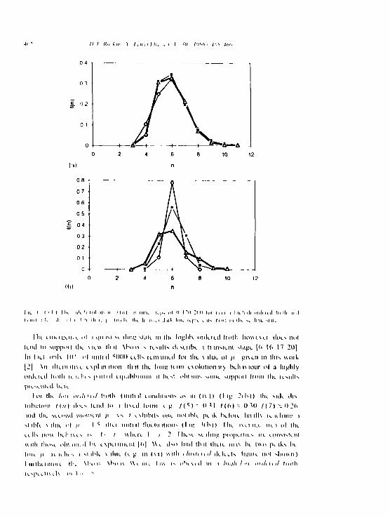
I l I /<» i n i 1 f x i t i ' l l w ii » l 4 \ ì j f i u

( 1 )

0 8

0 7

0 6

0 5

g 0 4

0 3

02

o 1 0 ••

0

I i l < ( i l i I l u ti li li I I il u h n M n I il U n i i K p*. o l •• I "'(I 2( 0 lu i ( \ i | i li i l li i li n u l i i n i I h ili im i

| \ m l i l i il i i I i l l i i l i k [ t n i K t lu li i \ k i i l n k lu t i u p i i i t i l s f \ n ) hi i I k s,. i I i ml ' I i l i

I l a e m e i l i L i n e ol i t | i i is i m l i m e s l . i k n i i l a l n g h l v o i d e i c d f i o l i i h o u e \ e t d o c s n o i

kml l o suppoil l l i L \ i e u ih it \ b o i v s re Mills d e s e n b e i ti inMcnl s t u o i e |6 16 \7 20) I n I i c l o n l \ 1 0 ' n f u n i i i l M ) ( ) 0 c e l l s i c i ì ì m i c c i l o i l l i c \ ì l u c o l / / _ g i \ c n i n l l u s u o i k

12 ] \ n i l k m i l n e c \ p l i n i t i o n i h il I h c I o n e t e m i c \ o l n t i o n i t y beh ìmout o l a l u g h l y

o r c i c ieli lioth le iiliis pumi c q u i l i h i m m il 1v_M oblimi some snppoil ( i o n i Ihe lesulls p i e s e O k d b e l i

I or thè /-m ih./i Ui/ ti olii (mitili umilinoli .»s m (i\)) (liy 2(h)) 1 he siile disI I ibttlion f i n ) doe*' tend lo i f i\ed loi in l g / ( ^ ) ' I M I / ( 6 ) - ( M 0 / { 7 ) 0 2 6

md thè seeoud moment /i \s / e\llibils one noi ible pe ik beloie h n ili\ leiehinu i si ihlc V line ol II I iltei mitili lineili ilioiis ( I m Mb)) Mie i\eiiLe nei o! ihe eells imu he h i\ e i'' I1 l ubere I / 2 Illese se ìllliu piopeMies n e eonsislelll uilh ihose obtniud In e\peliment |ii| \\ e il-o hnd ih it llieie ili l\ he tuo pe lks he loie fi le le he s i M ihlt \ lille U ¿! III (M| uitli illtsftiitl deleets limile noi shou n )I n r l h e M i i o i e l l i e \ b o u \ b i > i \ \ \ e m e I i u i^ o b e \ e d i l i i l i h f l i / m i m i / i n s'

n

H I Hu 1 "i ) / ■ n i ' I hi n i I " / / j

(.1) t

(b| t

I ii i i \ Imiu in i lut . l i i n . l ! u J i n k u >1 In ih h il l i mi t ) il v. I uj l ■) i i i 1 1 i i n1 nomi il is oppos d Io i|li M sl ihm. in in ouluul lioih dLjunds oii i!k iiiiii il su)l ilisii ihution f[n\ il iIk mnnhii of (IlIlvIs ,/ w ii h i Lorrcspondiiiü iIhlvIioM or lii(il d \ diiL /' (</') pttinlk dLtLrmmmy iIil dutiL o| disordir liolhs xvilli inili 11 diliils ol \ moiis ivpcs [21] cilhcr rtndomk suded or cInslerctl IU| nuv LOULvpond tu iIjl simt ;i hui i\hthit ddktml mthnu>ntit\ h, fun tont betöre i Im il si iic ! «>t L\impk ont oi morc pt.iks inj> lu obscivcd ioi /<•> \s i in iIil low oidLied Iroili dLpLndm . kspllIi\lI) on uliLthir deluls ni sLidid r mdomk or ilusiuid NlvliiIilIlss il Mil svsiciii si/l is hmn iftL nrdind heilt will IliuI lo t i l hc r ,i quisi sl llniL ot sl iIiml st iIl il i ndkss ol IIil min il loudilimis (IiIiuuim Ii insitnl IhIiuumii will lu oI>sli\hI Moilolli oui IlsuIis st il ul s| ili ii wliil». f, (,( \ is uound0 2 l l » l I s V s i e (11 l i p l o I l l i o i l s l l l d ( . l I I s l l l l s \ l I l l L I I I L K I S L S | ( H I l f l L S \ s l u i l M / L

u i d t L i l m ^ . ( l u l ( h e p i o p o i l n m o i d ^ u M l s u l d e k U s m iIk t " . u i l l l i o i h < k k i n n i K d u .

lliiLvhold \ ihn.in Lonlrisi )<>i hitfh oi /oh liisoithini 11 otli". (Iijjs <■ S) iIk suk dMi ihnlion

/ ( / ; ) i l w i\ s I I i k I s io i 11 \ l d lorni I l y / 1 ^ I ( H 2 / (<' I 0 / ( 7 ) ' (I 1 ,K )

will» i si ihk \ i I u l ol // i I 4 I liiis i I k disoukud hodi m du m iIuil' sl i r i l

llks [ \ K l \ U 111 U l 1 O l l l l i l I I s \ \ I I I I I lIllOUL'll I I W i l l i / I N v l l l l L l l I l L

/ / / Ht 1 III ) / Il I / h i , , I It ! n t I m

( I) I

III) t

I i s I I i ' h i I i l l i . I) I V I m u a il li m i l i 11 VI 1111 ( 11 I \ 11 1 1 I I \ i n 1 n i 11 1%

\ h<> i \ no i (he \ h i ) i \ W e n n h u »ppI \ h e n i c c o r d m ^ to ou i mmhi I i l i o n k M i l ls

nul in i i i i e c i i k i i t w i t h p n u o i i s u o i k (or ihstmU u tf l i o l h e v o l n l i o n | l (> 10 12 I l[ l l o u i _ \ e i ih«, so e i l l c d o u l e n d m i t i l i c o n d i t i o n ( / / 0 4 ) o h i m ie d b \ n v e i s c

d i l h i s i o i i | I 2 I -41 m I k t is i k s s , / im h </t 1 1 </ no t \ n i l s U l k t n i c l>\ on»

de I in 11 k m

C on^ c ip ie n O v m u n M i l t s M ip p o i t tin. i x i s i u i u ot i m m c i s i l s e l l i n g si u l u n s p c i

l i \ e o l s s s i t i n s i / l lo i i i i i M H i U i t t ! I i o t h h iscd o n i \ o r o n o i c o n s t r u c t io n \ \ c l ind

til il a \ s i h i s e i l l i c i i / " ' i ( / pe ik \ dm. ( f t 2 0 ) ih in ili il o h s u v i d loi in

i m / ( i , i l I m i h { I ij_ M h ) ) o i nu le ises m o n o t o n i e i l ls ( I n 7 ( h ) ) W h i l e i l i a c ippc i ls

10 I k n _ ie e n ien ( is to the loe it io n o l the / / pe ik d m It iL <»/ </ / . / , ; c ti l u ' ill

c \ o h i l i o n H ' e t i n s 11 k e l \ t l l i l it is n ie le lv I c o u k i d e a l s u i t lee pi le n o o k n o n M i k e the

pe d V i l iu s in. di l l i , l e n i | 2 t 2 11 ( I oí e \ im p l e u c o h i ni l i I n l I» pe ik ( sin li is ¡ i

Ì 0 ) Ini Ole <>> il, >t 11 11 otti t l inde l condit ion ( l \ ) ) w l i e n is lot the i l l \oi th n <1 Id ill I \ u

ol ire i V e e n h o l MU ill pe ik ( /I 2 0 ) Ol not le ) I Ills i l k es w ith lorn le I u o i k u In i c

11 u h f o u n d t o u s e r i p i d h l o i m i \ i t n u t n ( / » 2 n " ' i n d ; I 2 | f ( l l l l l C 1 l l l o K i l k p l k I l O l l l e III >11

/ / I Un k m ì f n i ! I In i I !') Jh 4 / /

A fi fi

\1' i i \ U v i i u I iw in i In 111 I i Mi I I

i»t moli, ili in mie pc ik l o r n vs tinic < ippe i ts to (k i p e c u l i u i i \ o ( thè o n / i m /

l i o t h m d \ \ c lu u l no e \ u t e n t e lo r m u l l i p k pc ik s |oi m \ ì / i mh «/< n ti v | \ / c m u c l i u t

' • unn i i l ed

5 ( miclusini i

H \ q u m i i l u i u ti lt iniount ol >>i,iu < h \ n ( i t i in ti lt mit i il 2 M ho ih s i iu t l u i t u t

l n \ e ic to n c i lc d ippnc i i t disc iep me ics in ih t st i lm y p io p e ih cs d e s u ib in g tilt l ioth

cvo lu l io n O l i r ducei Mimi! i l ion icMiIts loi i d i s u n i i n t i h n f i i l \ n i t h m l l io th i r t in

d i ! i t t i n t n l u i t l i tliose ol o r i g m i l t \ p t r m i t n l s ol S m ith [ l | md \ l n n \ [2 | iLspte t iM .lv

< )ur Im d m g s suppoi i ihe \ leu tlmt i qu im se i lm g si i le c \ (M s in ì h i t / hh <>/</<#<</ l io th

u h e ie ll i t su l t ( l islribution / { / / ) ( » * <r 12 ) (a id s lo h i \ t i h v t t l to m i u h c r e is f i n )

Idi i li n is t i U i i s k e u e d u i l h co i i ts p o n d m g u n lm i i tcd u i o u l l i ol f i l l o u c s c i i

m m t i s i l s t i l l i l i : si He. ts I t l n t \ t i l loi bolli lite n ,1 md l m \ i m i t i t t l t io lhs

u l ic K / | / ì ) 1 u s i h \ e d lo m i cor icspondmg lo i s \ s t u i i m \ m i n i isunptot ic \ itu t ol

f i ' \ A \tl<l it lo r i ì l l \ u t sugjjcst in i l l t i n i l i v t c \ p l m i l i o n loi llie t n K i e siili ol

A b o i \ 12 ] to ih t t Me et t in i in o n l t i n i li olii i loes ic Ihc m i q u i s i s c i l m g si ite as

opposcd lo ( ( i n s i e m e W t liso con t im i l in i (he A h o ix (o i \ h o n \ \ c i l i c i t i u s ipplv

o n l \ hi ilic oi dt it J l ioth

K ì l i m i c i s

| ! | < S S m i i i i ' k l il I n l u t u i.

P I l> \ \ l> n \ K n l l i ui ipl iv H I I M I ) 4

| >| I l | I w l h i I l u x \ | >1 i I l ' » l i ' IS

| l \ \ I i \ m I lu i M i 11 '■* I I

| > | 1 \ ( .1 l / l I s i ( ii n u l i S) IV in l * l i \ l k > \ I | I ‘»S i ih

p * | I Si i \ m i i i i l 1 \ ( il i / k i I l iv s R i \ I i I I < "* i I WS • i M I v

| | I ) U i u n u n i I V k i i i m <k l ’I i i l M » l H JS i M ' ì ' I ' b

IMI) W "ti Mi I M ktiiu I I Ini Mi 11 se I I Mi >

/ / / It h L i n ) I , n , i 11 In i, i I Ut i ><t I •> ' 4M>

I 11 J W i. K li», ri I ) i H K i m l J I k i r i n m k I ’ ll 11 M i j , U } ( I l , M i I I ^

l " | y ► 1 i 1k i I N i l il im i k N i k i l i m i i I ' l i t l M i . N ( I) ( I ) Ww

I I J I I k i i un i l i nu l I ) \ \ i. n i i ( o m p l l i \ s < urn m i in M l ( I ' ) ‘ )0 ) 7>

P j l ) \ U u r i nu t I I I n I ’ ln i M ij l i l t f 2 l l W l » > J 2 7

1 ' I I ' ( i l i / i i i M I ’ \ i n l i i m ni nu l ( • S ( in. si I ' l l 11 M i j. H ( 1 I I '> >U ) (' I ^

1 4 ) 1 H i n l t l i i m i I I A n i I 1 l i m i M i J i : 4 | | l ' l ' ) 2 | 2 1 1

t ^ ) l> V\ i u r i nu l N H u i i r ( n n t i i n p I ' l n s 2 s ( l ‘M 4 ) **>

I < j J \ ( 11 i / i i r nu l I ) \ \ i u n J I *11V s ( t i t i l l i n-« M l i t i i 4 (1 2 ) I *<(>7

1 7 1 J s t n n is R i p I i i 'l H i s s V» ( I \ ) ’ i l

I X J I ) \ \ i m i nu l M A I « m i s \ « k l ’ I i w 4 W 1 1, ' M > ì »k s

l ‘>) I I I i \ il i l i P l u s R i i I i tt 7 : ( | ‘W 4 ) 4 ( > W

I ) W u m l ’h ) s l u i 7 4 l l ‘M S ) * 7 1 0

2 I j 11 I R i i k in m û ^ I i n j . I l ' I n s ( m u l i ns M il tu i 7 ( I ) I ^ 1

2 ’ j 'i h m^. I (. M M m i i H a li im i I \ ( i l i / n r l ’ h vs R o I < 2 M ' > ‘> S ) R U H

2 í | I U m l t k I ' l l I ) I I k s i s ( l ‘> P »

1 11 H I i \ il in im i I D u m i i i i v I hi p l i v I i n *2 ( l I ^4 *

Usuici Si tener H \ MI nuli"

rcvncil

Appendix B t£fThis introduces the CA approach to scientific computing problems through a short illustrationExamples of Sequential and Mutli-spin coding methods for cellular automata methods are given as followsProgram Sequential uses sequential updating and the most recent value of the neighbour spins and, as such, is not strictly CA methodology as it is generally realised for very many similar elements, since it is inefficient, More usually, cellular automata use simultaneous or parallel updating, where each spin at time t+1 takes its neighbour values at time tProgram Multi2 uses multi-spin updating (details see Section 2 2 3 3) for square lattice A second index J is introduced besides the index I Many loops run over I and J A single logical function, OR is used here to implement that a spin is up if at least one of its four neighbours is up, and the OR rule is over all the four neighbours This achieved computing speeds which are much improved compared to the sequential method

PROGRAM SEQUENTIAL PARAMETER L=960,LP1=L+1)INTEGER MAX,ISEED,IP,IBM,I,ITIME,MAG LOGICAL N(O.LPl)REAL*4 PREAD(*,*)P,MAX,ISEEDIP=(2.0 *P-1 0)*2147483648.0IBM=2 *ISEED-1DO 10 1=1,L

IBM=IBM*16807 N (I)=IBM.LT IP

10 CONTINUEDO 100 ITIME=1,MAX

MAG=0DO 20 1=1,L

IF(N(I)) MAG=MAG+12 0 CONTINUE

WRITE(*,*)ITIME,MAG IF(MAG.EQ.L OR MAG EQ.0)STOP N (0)=N(L )N(LP1)=N(1)DO 30 1=1,L

N(I)=N(I-1) OR N(I+1)3 0 CONTINUE100 CONTINUE

STOPEND

B-l

PROGRAM MULTI2INTEGER L ,L W l ,LW,NBIT,NB,MAX,ISEED,IP,IBM,I,

J,ITIME,IDOWN,LTEMPl,LTEMP2

PAR A M E T E R (LW=3 0 ,LWl=LW+l,N B I T = 3 2 ,L=LW*NBIT,LPl=L+l) INTEGER N (0 LP1,0:LW1)INTEGER M (L ,L W )RE A L *4 PI S H F T C (I ,K ) = I O R (I S H F T (I ,K) ,I S H F T ( I', K-NBIT) ) R E A D (*, *)P,MAX,ISEED I P = (2 0*P-1.0)*2147483648.0 IBM=2*ISEED-1 DO 2 0 1=1,LW

DO 10 J = 1 ,L N(J , I)=0

10 CONTINUE2 0 CONTINUE

DO 5 0 N B = 1 ,NBIT DO 40 1=1,LW

DO 3 0 J = 1 ,LN (J ,I )=I S H F T ( N (J ,I ),1)IBM=IBM*16807I F (IBM.LT.IP)N(J,I)=IOR(N(J , I ) ,1)

CONTINUE CONTINUE

CONTINUEDO 2 00 ITIME=1,MAX

IDOWN=0 DO 12 0 1=1,LW

DO 110 J = 1 ,LI F ( N O T (N(J , I )).N E .0)IDOWN=IDOWN+l I F (IDOWN EQ 0)STOP

CONTINUE CONTINUEW R I T E (9,*)IT I M E ,IDOWN DO 13 0 1=1,LW

N( 0 , I)=N(L,I)N (L P l ,I )= N (1,1)

CONTINUE DO 140 J = 1 ,L

N (J , 0)= I S H F T C ( N (J,LW),NBIT-1)N(J,LWl)=ISHFTC(N(J,1),1)

CONTINUE DO 160 1=1,LW

DO 150 J = 1 ,LLTE M P l = I O R ( N (J ,1-1),N(J,1+1)) LTEMP2=IOR(N(J-l,I),N(J+l,I))M (J , I )=IOR(LTEMPl,LTEMP2)

r

CONTINUE

304050

110120

130

140

150

B-2

160

1701802 0 0

CONTINUE DO 180 1=1,LW

DO 170 J=1,L N(J,I)=M(J,I)

CONTINUE CONTINUE

CONTINUE STOP END

B-3

Appendix CThe various initial conditions of 2D froth with a single defect

C-l

C-2

f

r*'* T - (b)

Figs C-3 (a)(b) later stage o f froths evolution Note (a) initial structure is pairs of pentagonal-heptagonal

C-3

Appendix D

Some detailed results obtained from direct simulation

We include here example outputs of a system of size 900 cells After creating a Voronoi network containing 900 cells, the final network is given with statistics showing the distribution of the number of the cell sides with \i2 ~l 38 We only give the database obtained during time steps o f 80-160, the second moment, |l2, is thus approaching its final stable value

The results we obtained compared well with the results of Kermode and Weaire (1990) and overall agreement on the evolution was achieved with only minor difference in values quoted by those authors This was partly due to the fact that the values o f convergence CNVRMS and CNVRSD and scale factor SCALER were not the same (SCALER is the function of the long diagonal used in the hard-disk formulation in subroutine VSETUP, equivalent to the area perturbation scale in the further subroutine SETUP, see programme disk Appendix E)

D -l gives the results for vertices o f each cell o f the network, and the value o f pressure and area o f each cell and the area change value during the evolution Thetotal area and pressure are also given VI£

Tables D-2, D-3 and D-4 show the distribution of the cells with n sides, and calculate the second moment, and show the distributions of average area o f n- sided cells and average number of sides of neighbouring cells to n-sided cells They are used to test correlation laws due to Lewis and Aboav (Aboav-Weaire)

STEP 1 6 0 VERTEX

NO NEAREST VERTICES NEAREST CELLS FL X-COORD Y-COORD1 6 6 13 3 1 1092 6 1 3 64 3 109 15 73 4 2 1 109 14 3 5 9 3 5 1 2 5 55 59 4 12 1 4 7 8

12 5 13 16 82 4 7 813 15 12 1 1 1 0 61 4 1 6 15 77 6 9 1 17 215 13 7 0 14 6 9 1 8216 19 12 14 82 1 7 21 8 2 4 59 19 4 7 8 5 0 419 18 16 23 17 2 5 0 422 2 8 23 7 2 2 172 3 8 823 18 2 6 58 2 1 6 89 22 6 2 4 27 3 2 1 4 5 2 1 627 23 3 1 26 1 4 5 5 0 42 8 29 22 96 3 8 8 7 0 629 3 0 28 1 1 3 7 0 6 7 7 730 29 35 3 1 42 8 5 63 1 27 3 0 34 42 14 53 2 4 4 26 34 14 5 47 93 4 32 3 1 36 42 47 93 5 1 2 4 3 6 30 42 7 7 73 6 39 34 35 42 3 1 139 3 6 12 3 40 25 0 47 940 4 1 39 7 2 4 25 0 5 9 44 1 44 40 42 5 9 4 4 5 142 46 4 1 8 5 4 59 4 10 34 4 48 32 4 1 4 7 9 4 5 14 6 42 8 7 1 47 36 4 5 147 4 8 46 50 36 51 348 53 44 47 4 5 1 51 35 0 5 1 47 6 3 0 36 7 8 45 1 5 0 6 2 6 52 3 7 6 51 35 2 5 1 55 53 122 51 35 3 — ^ 4 8 52 58 12 2 2 1 65 5 6 2 3 56 52 122 3 7 65 6 60 57 55 122 40 657 59 58 56 12 2 2 5 55 8 53 57 24 89 2 2 1 6

2 4 3 2 4 2 2 4 4 2 5 3 8 68 22 4 4 1 1 2 2 1 1 2 9 2 4 3 8 4 1 02 4 6 2 5 0 2 6 1 2 4 1 13 2 3 4 72 5 0 2 5 1 2 4 6 2 4 2 34 7 68 22 5 1 2 5 2 2 5 9 2 5 0 16 68 22 5 2 2 5 3 2 6 8 2 5 1 3 1 6 68 22 5 3 2 5 2 2 4 3 1 1 3 3 8 46 32 5 9 2 6 5 2 6 0 2 5 1 16 3 1 6

1 0 6 14 2 3 5 7 8 5 23 9 1 1 7 8 37 7 6 1 4 8 6 2 4 4 4 2 6 9 0 5 4 4 91 5 7 15 3 7 6 7 9 7 2 5 2 2 4 6 6 315 7 1 6 6 4 0 1 9 6 2 4 9 0 4 9 0 02 5 5 16 9 8 1 8 6 3 2 3 0 0 0 4 0 8

1 1 6 4 2 5 5 0 5 22 5 8 8 6 9 082 14 5 1 5 1 3 2 23 1 5 7 7 4 782 1 4 4 2 3 8 5 0 2 0 9 3 3 3 1 7

1 0 6 13 6 6 5 3 8 2 2 2 0 0 5 4 4 04 7 8 1 6 4 9 6 3 8 2 2 1 8 2 7 1 0 889 2 17 7 4 8 8 4 2 22 1 3 2 5 1 74 7 8 1 6 9 9 3 9 8 4 2 1 5 8 7 9 1 78 5 6 15 9 6 8 5 0 2 18 5 0 5 5 8 150 4 18 7 9 5 8 1 3 2 1 8 0 7 2 9 35 0 4 19 3 5 9 3 1 2 19 4 1 1 8 5 48 5 6 18 9 8 7 6 3 3 19 0 9 1 4 4 48 5 6 1 6 0 2 5 3 6 0 1 6 9 4 3 3 4 28 5 6 17 0 1 5 6 1 0 16 2 2 9 1 2 077 7 19 3 0 8 0 8 3 17 2 3 3 7 4 685 6 19 5 1 4 8 2 4 17 8 8 9 3 6 62 1 6 2 0 1 1 7 7 7 5 1 8 9 5 0 6 7 21 4 5 19 7 4 2 0 6 0 17 8 9 5 3 4 43 1 1 1 9 7 2 4 1 0 0 1 6 9 6 8 4 7 747 9 19 9 9 3 6 6 8 17 1 6 0 5 4 03 1 1 2 1 2 7 0 6 7 4 1 6 3 3 1 9 0 547 9 22 4 1 3 2 5 6 1 6 6 2 7 1 9 347 9 2 2 7 8 3 4 8 9 1 8 . 7 5 4 5 8 34 5 1 23 8 0 7 7 0 3 19 4 7 0 9 8 92 1 6 2 1 6 8 9 4 2 6 19 5 4 7 4 2 610 3 23 8 6 2 8 2 7 2 0 5 4 5 9 1 84 5 1 2 3 2 0 4 5 3 8 2 1 2 9 5 2 2 32 1 6 2 1 9 8 9 8 6 2 2 1 0 2 0 2 1 251 3 2 3 7 5 7 2 0 2 2 2 7 9 5 8 8 17 8 4 22 6 5 8 4 8 2 2 3 9 8 7 2 3 63 7 6 2 0 9 7 8 9 1 0 2 3 5 6 9 7 9 851 3 20 6 1 2 0 5 3 22 5 6 5 6 1 540 6 19 8 5 3 8 1 7 2 4 9 0 0 9 2 72 5 5 19 5 3 9 1 3 5 2 4 8 6 7 8 3 489 2 1 8 . 7 7 0 4 2 4 2 3 0 4 1 7 0 812 2 19 2 2 6 2 8 6 22 4 3 4 1 9 14 1 0 6 4 6 2 6 4 4 3 6 6 3 9 7 7 17 3 6 6 3 1 7 1 9 0 3 8 4 3 3 0 2 5

16 7 8 3 2 2 9 8 3 4 2 3 7 3 5 416 7 4 1 5 3 5 3 3 4 4 7 1 5 2 3

3 1 6 5 8 4 3 4 2 5 33 6 0 4 5 3 446 3 4 9 4 8 9 4 5 3 4 1 1 8 9 6 168 2 4 8 7 0 4 5 0 3 5 6 3 5 2 1 26 4 2 5 7 8 1 8 1 3 32 4 9 3 8 3 2

ITERATION 6CELL

NO NS PRESSURE AREA1 6 -- 7 3 4 5 7 1 E - 0 1 4 9 2 1 4 2

3 6 0 4 4 6 8 2 8 E - 0 1 2 0 5 7 8 54 5 - 4 0 9 7 0 4 E - 0 1 4 2 4 8 6 27 5 0 3 9 9 7 7 7 0 5 7 2 3 3 58 7 - 1 4 0 4 5 8 9 1 7 2 0 0

10 4 0 4 5 9 7 5 9 0 9 2 6 2 4 711 6 - 2 5 1 9 0 0 E - 0 1 4 8 5 2 9 512 6 - 7 8 0 2 1 8 E - 0 1 4 5 1 5 9 51 4 6 - 9 0 0 6 2 6 E - 0 1 4 4 8 5 9 416 6 - 9 8 6 0 5 4 E - 0 1 4 1 6 6 9 022 9 - 2 2 6 3 8 7 1 1 3 7 6 823 5 0 3 0 3 5 7 1 0 7 2 3 3 3 22 4 6 - 1 0 9 8 5 9 2 2 8 5 5 92 6 8 - 2 4 4 1 3 5 1 1 9 5 3 22 7 5 0 4 8 1 5 2 9 E - 0 1 2 1 0 1 4 02 8 5 0 2 3 9 3 5 2 0 7 5 4 7 9 130 7 - 1 8 6 5 0 4 10 2 7 2 732 7 - 1 7 2 0 3 2 5 2 2 0 5 8

''^3 6 6 - 3 6 6 4 5 1 E - 0 1 3 3 8 4 4 139 7 - 1 9 0 8 5 7 9 6 4 7 5 142 5 0 3 2 8 2 0 8 0 4 2 8 8 1 2

1 6 5 6 - 8 0 3 3 2 8 E - 0 1 4 7 3 2 0 81 6 7 5 0 1 8 6 7 0 9 1 5 9 1 3 71 7 0 7 - 1 9 2 0 7 4 4 6 7 6 0 91 7 2 7 - 1 1 6 5 2 4 7 3 9 9 1 8

D -l

CHANGE 0 5 3 7 4 6 3 E - 0 30 6 6 7 4 2 1 E - 0 4- 1 3 6 3 3 7 E - 0 2- 1 0 4 7 5 6 E - 0 3- 2 2 8 3 6 0 E - 0 2- 4 4 2 7 0 2 E - 0 30 5 7 8 9 8 0 E - 0 3 0 4 1 8 4 4 4 E - 0 30 9 8 9 7 7 7 E - 0 40 4 1 9 4 2 1 E - 0 2- 9 5 9 5 4 8 E - 0 4

0 5 4 2 4 7 9 E - 0 3- 1 7 5 2 9 8 E - 0 2

0 2 2 6 2 2 1 E - 0 2- 5 4 3 9 5 0 E - 0 4

0 1 0 2 1 0 5 E - 0 3

0 1 9 7 3 4 3 E - 0 3- 6 2 7 2 3 2 E - 0 5- 1 0 1 5 8 3 E - 0 2- 1 6 0 6 7 1 E - 0 2- 2 4 5 2 9 6 E - 0 3

- 1 3 0 4 9 7 E - 0 3- 8 8 4 2 0 9 E - 0 3- 2 9 2 1 1 8 E - 0 3

0 3 3 1 4 8 1 E - 0 6

2 6 0 2 7 6 2 6 1 2 5 9 16 64 2 37 7 6 9 7 6 8 4 6 3 1 5 9 6 1 9 32 6 1 3 2 1 2 4 6 2 6 0 16 3 7 7 13 2 7 4 7 1 1 7 1 3 1 7 4 1 1 3 1 1 7 32 6 5 2 5 9 2 6 7 2 7 1 5 8 4 6 4 2 3 1 6 4 0 6 2 2 0 8 3 1 7 1 1 3 9 52 6 7 2 7 4 2 6 5 2 6 8 3 1 6 5 5 0 58 4 3 5 7 1 7 5 9 32 0 1 0 9 8 6 1 7 42 6 8 2 6 7 2 5 2 26 9 4 6 3 55 0 31 6 3 5 0 4 6 0 4 33 2 0 5 0 4 42 6 9 1 1 9 2 2 6 8 1 1 8 8 46 3 8 3 2 55 0 2 2 5 1 6 4 2 33 8 2 8 0 9 4 1 7 528 2 2 9 1 2 8 4 2 8 1 39 7 8 8 0 2 8 0 7 7 7 5 9 3 3 27 5 7 5 9 9 3 18 82 8 4 2 8 5 2 8 2 3 1 4 2 8 0 57 0 39 7 8 3 9 2 8 7 2 2 8 7 4 0 2 2 12 8 5 2 8 4 3 2 1 2 7 6 3 7 7 3 9 7 57 0 7 5 2 6 3 4 2 3 0 7 6 0 2 4 1 18 92 8 6 2 8 1 2 7 8 2 8 8 77 3 8 8 0 81 3 5 2 2 9 8 3 0 27 1 8 2 6 8 42 8 8 2 8 6 2 9 8 2 8 9 84 3 8 8 0 7 7 3 5 3 4 6 9 9 9 2 5 8 0 6 3 4 3 19 02 8 9 2 8 8 2 9 5 3 0 2 84 0 8 8 0 843 6 2 3 7 4 8 5 2 5 3 7 1 2 6 92 9 1 3 0 2 3 1 5 2 8 2 2 8 0 8 8 0 87 5 8 2 8 4 8 7 7 2 6 7 9 7 7 0 5 1 9 12 9 5 3 0 1 2 8 9 2 9 7 84 3 3 1 4 84 0 6 1 4 9 0 6 1 2 4 4 0 0 8 6 22 9 7 2 9 8 2 9 9 2 9 5 3 1 4 8 4 3 90 0 5 2 1 5 4 9 2 23 9 9 7 9 5 2 19 2

1 7 0 7 1 7 0 8 1 6 6 0 1 7 0 6 98 7 4 4 8 1 0 38 0 5 6 2 7 4 12 3 0 1 3 7 9 8 6 51 7 0 8 1 7 0 7 1 6 9 7 1 6 5 1 2 3 7 8 1 0 74 4 37 8 5 4 0 7 6 12 5 2 9 1 3 51 7 1 0 1 7 0 6 1 7 0 3 1 6 9 7 3 5 1 7 4 4 193 38 4 5 2 9 2 7 13 0 8 9 3 0 1 86 71 7 1 1 1 7 1 4 1 7 0 3 1 7 1 2 1 9 3 6 5 6 40 8 4 0 3 5 1 8 2 2 15 3 8 5 7 3 61 7 1 2 1 3 4 6 1 3 4 7 1 7 1 1 6 5 6 19 3 7 5 1 41 7 1 6 4 9 9 14 9 9 2 0 1 9 8 6 81 7 1 4 1 7 1 8 1 7 1 9 1 7 1 1 4 0 8 6 5 6 6 3 3 4 0 3 3 9 6 5 7 1 5 . 7 8 6 5 4 91 7 1 6 1 7 0 3 1 7 1 9 1 6 9 4 24 9 3 5 1 40 8 39 6 1 8 0 1 1 15 5 4 4 5 1 9 8 6 91 7 1 8 1 7 1 4 1 3 4 7 1 7 2 0 7 7 5 6 3 3 65 6 4 0 9 1 4 4 9 4 1 6 1 5 0 9 4 01 7 1 9 1 7 2 2 1 7 1 6 1 7 1 4 4 0 8 6 3 3 2 4 9 39 9 2 8 7 6 4 15 9 3 1 3 8 5 87 21 7 2 0 1 7 1 8 1 6 2 2 1 7 2 1 49 0 63 3 7 7 5 40 7 5 6 3 2 5 17 4 7 7 0 6 61 7 6 2 1 7 6 8 9 9 5 1 7 6 3 2 5 4 8 6 1 49 1 4 8 0 6 2 0 6 5 1 0 6 4 1 7 1 01 7 6 3 1 7 5 8 1 7 6 4 1 7 6 2 8 6 1 2 5 4 1 2 1 47 4 0 6 7 1 5 1 1 2 9 5 6 5 1 8 8 817 64 17 63 1 3 4 9 1 3 6 3 8 9 1 8 6 1 1 2 1 4 5 1 2 8 1 5 9 1 1 4 0 1 8 4 51 7 6 6 1 7 6 7 1 3 5 6 1 7 7 0 5 2 7 6 0 4 8 6 1 45 1 9 2 1 5 4 8 6 6 8 9 0 5 8 8 91 7 6 7 1 7 6 8 1 7 6 6 1 7 7 1 6 0 4 7 3 7 8 6 1 4 6 4 0 0 4 5 5 8 2 5 2 0 3 11 7 6 8 1 7 6 7 9 8 1 1 7 6 2 4 9 1 8 6 1 7 3 7 47 9 6 5 1 6 4 9 2 2 4 2 9 0 8 9 11 7 6 9 1 3 4 9 1 7 6 0 1 3 3 7 5 7 7 18 9 1 2 1 4 6 9 1 9 7 5 8 1 4 1 6 8 5 9 11 7 7 0 1 3 7 6 1 3 8 3 1 7 6 6 6 0 4 52 7 5 3 0 44 8 9 5 8 8 2 8 3 1 4 5 3 7 8 9 21 7 7 1 1 7 6 7 1 3 8 3 1 7 8 8 3 4 8 7 3 7 6 0 4 46 1 2 3 4 0 9 6 9 0 9 4 6 61 7 7 4 1 2 1 2 9 7 6 1 7 7 5 5 5 6 7 2 0 7 56 51 8 8 3 0 4 5 4 7 8 3 6 0 0 8 9 51 7 7 5 1 7 7 4 1 7 7 6 1 7 7 8 4 2 8 7 2 0 ' 5 5 6 5 1 0 6 4 6 6 7 4 4 4 9 3 1 01 7 7 6 9 8 2 1 7 7 9 1 7 7 5 4 2 8 5 5 6 7 3 7 49 7 1 5 0 2 7 5 3 9 0 6 5 4 8 9 61 7 7 8 1 2 1 1 1 7 7 5 1 4 6 8 4 2 8 5 8 8 7 2 0 5 1 0 8 3 3 7 8 3 9 9 0 7 2 31 7 7 9 1 7 7 6 1 7 8 8 1 4 6 7 1 5 8 4 2 8 7 3 7 48 2 5 9 8 8 4 4 6 7 9 5 5 8 8 9 71 7 8 0 1 4 6 0 1 4 6 1 1 2 1 0 8 6 8 5 8 8 489 5 1 1 0 5 1 5 6 0 67 4 7 6 71 7 8 8 1 7 7 1 1 3 9 1 1 7 7 9 1 5 8 7 3 7 3 4 8 46 7 5 2 8 9 2 5 3 9 5 4 9 8 8 9 81 7 8 9 1 1 6 0 1 1 3 8 1 1 4 6 63 5 5 8 3 8 4 5 1 7 4 2 7 5 2 39 3 2 2 7 0 81 7 9 4 1 7 9 7 1 3 8 0 1 6 7 0 19 2 2 6 8 4 4 7 39 1 1 1 5 6 8 5 9 4 8 7 9 1 9 0 01 7 9 7 1 3 8 7 1 7 9 4 1 6 7 4 2 6 8 5 4 2 447 39 2 3 9 1 5 9 5 4 2 9 9 3 5

TOTAL AREA 2 3 3 8 27 TOTAL PRESSURE 0 6 8 5 4 5 3 E - 0 6

5 0 2 4 4 2 8 96 0 1 2 3 7 9 7 E6 - 17 2 8 2 9 E -7 - 1 2 6 8 5 7

5 0 3 0 2 5 2 74 0 4 9 0 2 1 68 - 2 1 8 7 8 85 0 1 5 6 5 8 75 0 40 3 6 9 5 E -6 - 1 5 7 1 7 3

8 - 2 4 7 0 3 87 - 1 4 3 5 6 7

6 - 1 2 7881 6 1 3 4 3 6

0 5 7 8 8 4 6

-0 1 2 5 1 0 6 0•01 3 8 6 9 6 4

5 6 8 8 3 1 0 3 8 9 2 1 8

0 6 3 8 7 8 4

13 1 5 6 9

1 1 6 6 5 9

0 1 2 6 4 2 9 04 2 6 3 7 8

9 6 2 4 5 1

8 5 8 8 9 2

- 2 8 3 4 6 3 E - 0 4

0 3 3 7 3 7 3 E - 0 3

0 2 6 4 9 1 5 E - 0 2- 4 7 9 7 7 3 E - 0 4- 4 5 7 8 0 8 E - 0 4- 7 6 7 1 3 9 E - 0 4- 7 1 3 8 2 0 E - 0 3- 1 5 5 6 9 6 E - 0 4

0 9 4 0 5 0 9 E - 0 3- 3 8 7 2 3 7 E - 0 4- 8 8 6 6 8 0 E - 0 3- 3 4 7 7 3 3 E - 0 2

0 3 7 8 2 7 2 E -0 2

6 - 1 3 3 1 6 2 8 7 7 7 5 36 0 3 9 0 2 8 6 E - 0 2 3 9 9 8 0 65 0 2 1 8 2 3 5 0 9 8 9 0 1 15 0 1 4 7 7 9 4 1 2 6 6 4 48 - 2 5 6 3 4 2 9 0 2 7 0 7-8 - 1 8 9 7 7 8 1 1 6 2 1 66 - 4 4 9 8 6 1 E - 0 1 3 4 6 7 7 46 - 7 8 9 6 1 6 E - 0 1 2 3 6 3 6 57 - 1 5 5 4 8 3 1 1 6 6 8 8

- 2 1 4 5 1 3 E - 0 2

0 1 2 2 7 8 8 E - 0 2

0 9 6 4 9 2 7 E - 0 6

0 9 1 3 1 4 2 E - 0 4

0 6 1 4 6 8 5 E - 0 3

0 7 0 8 2 3 0 E - 0 4

0 7 1 5 6 2 0 E - 0 4

0 7 4 7 7 6 0 E - 0 3- 4 5 8 8 8 5 E - 0 2

NUMBER CELLS REMAINING 50 9

D-2

IN IT IA L CONFIGURATION 60 BY 3 0 SYSTEM ------- > 1 8 0 0 VERTICES , 9 0 0 CELLSCONVERGENCE (EQUIL) - 0 5 0 0 0 E - 0 2 TOLERENCE (DIFFUS) - 0 OOOOE+OO

OPTIONS --------> 0 , 0 , 0 , 0 , 0 , 0 , 0 , 0 , 0 , 0 , 0 , 0 , 0 , 0 , 0 , 2 , 0 , 0 , 0 , 0NUMBER STEPS PERFORMED - 1 6 0 FINAL CELL COUNT - 5 0 9 NUMBER OF TOPOLOGICAL CHANGES----------- > T1 - 3 4 2 T2 - 1 8 1

PROGRAM R O U T E > SYSTEM PERIODIC /IN PU T - FOR 3 1 DAT /EQUIL CALLS - 80 DIFFUS CALLS - 84STATISTICS - - - - - - - - - - - - TABLE A

D i s t r i b u t i o n o f t h e n u m b er o f c e l l s w i t h n s i d e s o v e r 1 6 0 s t e p s s h o w i n g 80 p o i n t sSTEP I 3 4 1 5 1 6 1 7 1 8 1 9 1 10 1 1 1 1 12 I TOTAL 1 NO T1 MU2

8 1 1 0 33 1 2 0 9 1 2 5 1 1 1 3 5 1 45 1 1 1 1 3 1 1 1 0 1 68 8 1 3 1 2 0 382 1 0 29 1 2 1 4 1 2 4 7 1 1 3 6 1 43 1 11 1 3 1 1 1 0 1 6 8 4 1 5 1 1 8 483 1 0 27 1 2 1 4 1 2 4 7 1 1 3 5 1 43 1 10 1 3 1 1 1 0 1 6 8 0 1 4 1 1 6 5

1 1 9 1 0 29 1 19 0 1 2 0 2 1 1 3 0 1 39 1 9 1 2 1 1 1 0 1 60 2 1 14 1 2 1 31 2 0 1 1 27 1 1 8 8 1 2 0 1 1 1 3 3 1 39 1 7 1 2 1 1 1 0 1 59 9 1 7 1 1 9 21 2 1 1 0 28 1 18 7 1 2 0 2 1 1 2 8 1 42 1 6 1 2 1 1 1 0 1 5 9 6 1 7 1 1 8 51 2 2 1 2 24 1 18 8 1 2 0 0 1 1 3 0 1 39 1 7 1 2 1 1 1 0 1 5 9 3 1 6 1 1 9 41 2 3 I 0 24 1 1 9 0 1 2 0 0 1 1 2 8 1 41 1 5 1 2 1 1 1 0 1 5 9 1 1 0 1 1 5 11 2 4 1 1 22 1 192 1 19 7 1 1 2 7 1 42 1 5 1 2 1 1 1 0 1 58 9 1 5 1 1 6 51 2 5 I 0 2 1 1 1 9 2 1 2 0 0 1 1 2 5 1 42 1 4 1 2 1 1 1 0 1 5 8 7 1 1 1 1 2 81 2 6 I 1 19 1 1 9 1 1 2 0 1 1 1 2 2 1 42 1 4 1 2 1 0 1 1 1 58 3 1 6 1 14 91 2 7 1 0 17 1 19 3 1 1 9 9 1 1 1 8 1 42 1 4 1 2 1 1 1 0 1 5 7 6 1 7 1 1 1 11 2 8 1 2 14 1 1 9 4 1 19 7 1 1 1 9 1 42 1 4 1 2 1 1 1 0 1 5 7 5 1 3 1 1 2 71 5 4 1 0 26 1 1 6 0 1 1 8 0 1 1 0 9 1 37 1 7 1 2 1 0 1 0 1 5 2 1 1 3 1 1 8 21 5 5 1 1 25 1 1 6 0 1 1 8 0 1 1 0 7 1 3 8 1 6 1 3 1 0 1 0 1 5 2 0 1 2 1 2 1 21 5 6 I 2 25 1 1 5 8 1 18 3 1 98 1 39 1 10 1 2 1 0 1 0 1 5 1 7 1 16 1 2 6 11 5 7 1 0 25 1 1 5 8 1 1 8 5 1 99 1 37 1 9 1 2 1 0 1 0 1 5 1 5 1 0 1 2 0 01 5 8 1 1 24 1 15 7 1 18 7 1 96 1 38 1 8 1 3 1 0 1 0 1 5 1 4 1 2 1 2 2 61 5 9 1 1 22 1 15 9 1 1 8 5 1 9 8 1 36 1 8 1 3 1 0 1 0 1 5 1 2 1 3 1 2 0 71 6 0 I 0 20 1 1 6 1 1 1 8 5 1 98 1 34 1 9 1 2 1 0 1 0 1 50 9 I 2 1 1 5 5

D-3

STATISTICS - - - - - - - - - - - - TABLE BDistribution of the average area of n-sided cells over 160 steps showing 80 points

STEP 1 3 1 4 1 5 1 6 1 7 1 8 1 9 1 10 1 11 1 128 1 10 OOOOE+OO 1 0 4 3 2 2 1 1 42 8 1 3 3 3 4 1 5 3 0 6 1 7 3 6 6 1 8 57 3 1 10 84 1 14 09 0 00 E + 0 082 10 OOOOE+OO 1 0 4 6 4 4 1 1 42 3 1 3 3 6 9 1 5 3 6 0 1 7 3 8 3 1 8 61 7 1 10 90 1 14 16 0 00 E + 0 083 10 0 0 0 0 E + 0 0 10 5 6 7 7 1 1 419 1 3 3 9 5 1 5 3 7 3 1 7 46 4 1 8 7 2 4 1 10 94 1 14 20 0 0 0 E + 0 08 4 10 0 0 0 0 E + 0 0 10 5 7 1 1 I 1 40 9 I 3 3 9 6 I 5 3 8 8 I 7 6 3 0 I 8 8 8 6 I 10 2 5 I 14 3 1 0 0 0 E + 0 0

89 10 OOOOE+OO 10 6 1 1 7 I 1 4 1 1 I 3 4 2 4 I 5 5 0 2 I 7 5 1 5 I 9 6 4 1 I 10 5 1 I 14 65 10 OOOOE+OO I1 3 8 10 OOOOE+OO 1 0 4 4 9 8 1 1 72 2 1 3 9 7 5 1 6 78 7 1 9 6 1 0 1 10 30 1 17 27 10 0 0 0 0 E + 0 0 113 9 10 OOOOE+OO 10 3 7 9 1 1 1 7 5 5 1 3 9 7 5 1 6 82 2 1 9 43 4 1 10 39 1 17 38 10 0 0 0 0 E + 0 0 11 4 0 10 2 1 1 8 E - 0 1 1 0 5 2 1 0 1 1 81 7 1 4 0 1 4 1 6 7 7 1 1 8 9 5 1 1 11 53 1 16 43 1 0 0 0 0 0 E + 0 0 11 4 1 1 0 8 1 1 3 E - 0 1 10 4 0 2 7 1 1 80 0 1 4 0 4 0 1 6 7 7 2 1 9 8 6 0 1 11 46 1 16 70 1 0 0 0 0 0 E + 0 0 114 2 10 8 2 9 1 E - 0 3 10 5 5 3 2 1 1 809 1 4 04 9 1 6 8 4 0 1 9 8 1 9 1 12 29 1 14 54 10 0 0 0 0 E + 0 0 114 3 10 OOOOE+OO 10 6 0 3 7 1 1 807 1 4 06 5 1 6 8 8 8 1 9 9 8 1 1 12 06 1 16 87 10 0 0 0 0 E + 0 0 114 4 10 1 4 5 1 E - 0 1 10 6 9 9 2 1 1 819 1 4 02 8 1 6 9 3 0 1 10 06 1 11 63 1 16 90 10 0 0 0 0 E + 0 0 1

1 5 1 10 OOOOE+OO 1 0 7 3 4 9 1 1 869 1 4 0 7 2 1 7 13 9 1 10 27 1 12 86 1 17 44 10 0 0 0 0 E + 0 0 115 2 1 0 OOOOE+OO 1 0 7 1 4 7 1 1 85 8 1 4 07 2 1 7 14 9 1 10 29 1 12 89 1 17 48 10 0 0 0 0 E + 0 0 11 5 3 10 OOOOE+OO 10 8 2 9 7 1 1 9 0 0 1 4 06 0 1 7 12 7 1 10 34 1 12 51 1 17 51 10 0 0 0 0 E + 0 0 11 5 4 10 OOOOE+OO 10 8 4 7 8 1 1 909 1 4 0 6 3 1 7 09 4 1 10 28 1 12 94 1 17 54 10 0 0 0 0 E + 0 0 11 5 5 1 0 2 4 2 1 E - 0 1 10 8 5 0 3 1 1 8 8 8 1 4 0 9 6 1 7 10 6 1 10 28 ■ —

* h* iti 23 1 15 7 1 10 0 0 0 0 E + 0 0 1

1 5 6 10 2 2 8 9 E - 0 1 10 7 5 8 1 1 1 86 3 1 4 2 1 1 1 7 2 2 5 1 9 9 1 4

1 <N 1 H 1t- —

■I111

3 8 1 17 87 10 0 0 0 0 E + 0 0 115 7 10 OOOOE+OO 1 0 7 3 2 7 1 1 85 0 1 4 2 2 1 1 7 2 3 3 1 10 26 1 12 81 1 17 93 10 0 0 0 0 E + 0 0 11 5 8 10 2 1 0 9 E - 0 1 10 7 9 4 5 1 1 84 8 1 4 2 4 7 1 7 2 4 0 1 10 22 1 13 2 6 1 15 12 10 0 0 0 0 E + 0 0 11 5 9 1 0 3 7 8 1 E - 0 1 10 8 2 3 8 1 1 8 5 8 1 4 2 4 5 1 7 3 0 1

1 O I

1 H l

1 l

t- — -

1

32 1 12 84 1 16 48 10 0 0 0 0 E + 0 0 11 5 0 1 0 OOOOE+OO 10 8 7 7 5 1 1 867 1 4 2 5 4 1 7 40 7 1 10 43 1 12 94 1 18 09 10 OOOOE+OO 1

D-4

STATISTICS TABLE CDistribution of the average number of sides of cells neighbouring n-sided cells over 160 steps showing 80 points

STEP I 3 I 4 I 5 I 6 I 7 I 8 I 9 I 10 I 11 I 128 1 10 OOOOE+OO 1 6 8 7 1 1 6 432 1 6 2 0 3 1 6 0 2 8 1 5 9 0 6 1 5 8 0 8 1 5 63 3 1 5 4 5 5 0 0 0 0 0 E + 0 0

82 10 OOOOE+OO 1 6 879 1 6 430 1 6 1 9 8 1 6 0 3 4 1 5 8 8 1 1 5 7 9 8 1 5 6 3 3 1 5 45 5 10 OOOOE+OC83 10 OOOOE+OO 1 6 9 2 6 1 6 417 1 6 1 9 8 1 6 0 3 1 1 5 8 9 0 1 5 7 8 9 1 5 5 6 7 1 5 4 5 5 1 0 0 0 0 0 E + 0 084 10 OOOOE+OO 1 6 9 5 5 1 6 4 1 5 1 6 2 0 0 1 6 0 2 4 1 5 9 0 5 1 5 8 1 5 1 5 5 5 0 1 5 45 5 1 0 OOOOE+OO85 10 0 0 0 0 E + 0 0 1 6 9 6 3 1 6 413 1 6 1 9 7 1 6 0 2 6 1 5 9 0 2 1 5 8 1 5 1 5 5 5 0 1 5 4 5 5 1 0 OOOOE+OO

8 6 10 0 0 0 0 E + 0 0 1 6 9 7 2 1 6 413 1 6 1 9 4 1 6 0 2 0 1 5 90 9 1 5 8 4 0 1 5 6 0 0 1 5 4 5 5 1 0 0 0 0 0 E + 0 087 10 0 0 0 0 E + 0 0 1 6 96 3 1 6 41 6 1 6 1 9 5 1 6 0 2 0 1 5 89 9 1 5 83 3 1 5 6 0 0 1 5 45 5 1 0 0 0 0 0 E + 0 0

8 8 1 7 0 0 0 11 6 9 4 4 1 6 424 1 6 1 9 6 1 6 0 2 5 1 5 9 0 5 1 5 889 1 5 6 0 0 1 5 4 5 5 1 0 OOOOE+OO

1 3 2 10 0 0 0 0 E + 0 0 11 7 0 2 1 1 6 399 1 6 1 9 3 1 5 9 8 9 1 5 9 3 8 1 5 7 6 2 1 5 9 0 0 1 5 54 5 1 0 OOOOE+OO

1 3 3 1 8 0 0 0 11 7 1 1 5 1 6 409 1 6 2 1 0 1 5 9 9 2 1 5 9 3 6 1 5 7 7 8 1 5 8 0 0 1 5 5 4 5 1 0 OOOOE+OO1 3 4 10 OOOOE+OO 11 7 0 0 0 1 6 393 1 6 2 0 2 1 5 9 9 2 1 5 9 0 8 1 5 7 6 4 1 5 8 3 3 10 OOOOE+OO 1 0 OOOOE+OO1 3 5 10 0 0 0 0 E + 0 0 1 7 0 2 1 1 6 3 9 1 1 6 2 0 0 1 5 9 9 2 1 5 9 0 2 1 5 7 6 4 1 5 8 3 3 10 0 0 0 0 E + 0 0 1 0 OOOOE+OO

1 5 0 10 OOOOE+OO 1 6 91 2 1 6 44 4 1 6 1 8 4 1 5 9 9 0 1 5 8 9 6 1 5 7 6 2 1 5 8 5 0 10 OOOOE+OO 1 0 OOOOE+OO1 5 1 10 0 0 0 0 E + 0 0 1 6 893 1 6 456 1 6 1 8 0 1 5 9 9 9 1 5 8 7 8 1 5 7 4 6 1 5 8 0 0 10 0 0 0 0 E + 0 0 1 0 0 0 0 0 E + 0 0

1 5 2 10 OOOOE+OO 1 6 89 3 1 6 45 6 1 6 1 8 0 1 5 99 9 1 5 8 7 8 1 5 7 4 6 1 5 8 0 0 10 OOOOE+OO 1 0 OOOOE+OO1 5 3 10 0 0 0 0 E + 0 0 1 6 927 1 6 46 5 1 6 1 8 1 1 6 0 0 4 1 5 87 9 1 5 7 5 0 1 5 8 0 0 10 OOOOE+OO 1 0 OOOOE+OO1 5 4 10 0 0 0 0 E + 0 0 I 6 90 4 1 6 466 1 6 1 8 3 1 6 0 0 8 1 5 8 7 8 1 5 7 6 2 1 5 8 0 0 10 OOOOE+OO' 1 0 0 0 0 0 E + 0 01 5 5 1 8 3 3 3 I 6 9 4 0 1 6 4 6 6 1 6 18 7 1 6 O i l 1 5 8 8 5 1 5 7 4 1 1 5 8 3 3 10 OOOOE+OO 1 0 OOOOE+OO

1 5 6 1 7 8 3 3 I 6 9 6 0 1 6 470 1 6 2 1 1 1 6 0 1 6 1 5 8 6 5 1 5 7 4 4 1 5 8 0 0 10 OOOOE+OO 1 0 OOOOE+OO1 5 7 10 0 0 0 0 E + 0 0 I 6 9 3 0 1 6 462 1 6 19 9 1 6 0 0 6 1 5 8 6 5 1 5 7 4 1 1 5 8 0 0 10 0 0 0 0 E + 0 0 1 0 OOOOE+OO

1 5 8 1 8 0 0 0 I 6 9 7 9 1 6 464 1 6 1 9 8 1 6 0 1 0 1 5 8 7 5 1 5 7 6 4 1 5 7 3 3 10 OOOOE+OO 1 0 OOOOE+OO1 5 9 1 8 0 0 0 I 6 943 1 6 459 1 6 1 9 6 1 6 01 3 1 5 8 6 5 1 5 7 5 0 1 5 8 0 0 10 OOOOE+OO 1 0 OOOOE+OO

1 6 0 10 0 0 0 0 E + 0 0 I 6 9 3 8 1 6 4 4 8 1 6 1 8 6 1 6 0 0 9 1 5 8 6 0 1 5 7 6 5 1 5 8 0 0 10 0 0 0 0 E + 0 0 1 0 OOOOE+OO

D-5

Appendix £

Diskette ASandpile for — Sandpile Model program

Dissand for — Dissipative Sandpile Model programZz for Direct Simulation programPlan c ------Graphics programMe fo r MC method program

¡i

Documents

Computer Modelling of Complex Systems with Applications in Physical …doras.dcu.ie/18698/1/Yu_Feng.pdf · 2018-07-19 · 1 Computer Modelling of Complex Systems with Applications