Embed Size (px)
Citation preview

COMPUTER MODELING OF SINTERING IN CERAMICS
by
Alice C. De Bellis
B.S. in Engineering Mechanics, The Johns Hopkins University, May 1989
Submitted to the Graduate Faculty of
The School of Engineering in partial fulfillment
of the requirements for the degree of
Master of Science in Mechanical Engineering
University of Pittsburgh
2002
UNIVERSITY OF PITTSBURGH
SCHOOL OF ENGINEERING
This thesis was presented
by
Alice Cleveland De Bellis
It was defended on
June 20, 2002
and approved by
Patrick Smolinski, Associate Professor, Department of Mechanical Engineering
Ian Nettleship, Associate Professor, Department of Materials Science and Engineering
Thesis Advisor: William S. Slaughter, Associate Professor, Department of Mechanical Engineering
ii
ABSTRACT
COMPUTER MODELING OF SINTERING IN CERAMICS
Alice C. De Bellis, M.S.
University of Pittsburgh, 2002
A computer model of the sintering process has been developed to study the
evolution of the microstructure in a sintered part as a function of the volumetric density.
The model of the sintering process begins with a particle packing model, which generates
a close-packed array of particles. A Representative Volume Element (RVE) of the
packing is selected and examined. Next is densification, which is simulated by uniformly
increasing the radii of the particles.
Two dimensionless parameters, the intercept ratio Λ and the surface area ratio Ψ,
are used to quantify the model. This model shows good results at lower packing
densities. Areas in which the model can be improved and extended are also highlighted.
The intent of this model is to predict the final microstructure of a sintered part
based on its geometry and its stereology. It treats the sintering process as continuous,
without the stages normally used to describe sintering.
KEYWORDS Sintering
Particle packing
Powder metallurgy
Dimensionless parameters
Densification
Microstructure
Modeling
Stereology
iii
iv
ACKNOWLEDGEMENTS
I would like to thank my adviser, Dr. William Slaughter, for his guidance and
support in this endeavor. I would also like to thank Dr. Ian Nettleship of the Materials
Science and Engineering Department, for helping me understand the sintering process,
and fellow graduate students Jesus Ameneiro and Rich McAfee for their encouragement
and assistance. Finally, many thanks to Kumar Krishnan for providing the foundation on
which I could build.
This work is dedicated to my husband Michael.

v
TABLE OF CONTENTS
ABSTRACT....................................................................................................................... iii
ACKNOWLEDGEMENTS............................................................................................... iv
TABLE OF CONTENTS.................................................................................................... v
LIST OF TABLES............................................................................................................ vii
LIST OF FIGURES ......................................................................................................... viii
1.0 INTRODUCTION .................................................................................................. 1
1.1 Sintering.............................................................................................................. 1
1.2 The Sintering Process ......................................................................................... 2
1.2.1 Driving Energy and Mass-Transport Mechanisms ..................................... 2
1.2.2 Initial Neck Growth .................................................................................... 6
1.2.3 Intermediate Stage Sintering....................................................................... 6
1.2.4 Final Stage Sintering................................................................................... 8
1.3 Measurement Techniques ................................................................................... 8
1.3.1 Definitions................................................................................................... 8
1.3.2 Stereology ................................................................................................... 9
1.3.2.1 Calculating the Packing Density............................................................. 9
1.3.2.2 Calculating the Grain Size .................................................................... 10
1.3.3 Internal Surface Area Parameters ............................................................. 11
1.3.4 Dimensionless Parameters ........................................................................ 12
2.0 PARTICLE PACKING......................................................................................... 13
2.1 Particle Shapes.................................................................................................. 13
2.2 Particle Size Distributions ................................................................................ 14
2.2.1 Mono-Dispersed Spheres .......................................................................... 14
2.2.2 Binary Mixtures ........................................................................................ 15
2.2.3 Log-Normal Distribution .......................................................................... 16
2.3 Particle Packing Models ................................................................................... 17
3.0 PREVIOUS SINTERING MODELS ................................................................... 20

vi
4.0 DESCRIPTION OF MODEL ............................................................................... 22
4.1 Initial Packing and Rearrangement................................................................... 22
4.2 Selection of Representative Volume Element (RVE)....................................... 24
4.3 Densification..................................................................................................... 25
4.4 Computer Software and Hardware ................................................................... 26
5.0 RESULTS ............................................................................................................. 28
6.0 DISCUSSION....................................................................................................... 34
7.0 CONCLUSIONS................................................................................................... 37
8.0 DIRECTIONS FOR FUTURE RESEARCH........................................................ 38
8.1 Refining the Particle Packing Model ................................................................ 38
8.2 Simulating Different Sintering Conditions ....................................................... 39
APPENDIX A................................................................................................................... 40
SIMULATION CODE DESCRIPTION AND ALGORITHMS.................................. 40
APPENDIX B ................................................................................................................... 58
THE LOG-NORMAL DISTRIBUTION...................................................................... 58
APPENDIX C ................................................................................................................... 61
MONTE CARLO INTEGRATION.............................................................................. 61
BIBLIOGRAPHY............................................................................................................. 71

vii
LIST OF TABLES Table 1. The Classic Stages of Sintering. .......................................................................... 4

viii
LIST OF FIGURES
Figure 1. Neck Formation. ................................................................................................. 4
Figure 2. Coarsening Resulting from Low Coordination Number. ................................... 7
Figure 3. Calculating the Packing Density. ..................................................................... 10
Figure 4. Calculating the Mean Intercept Size................................................................. 11
Figure 5. Formation of Bridging Structures in a Random Packing. ................................ 15
Figure 6. Binary Mixture of Powders. ............................................................................. 16
Figure 7. Selection of Representative Volume Element (RVE). ..................................... 25
Figure 8. Packing Density versus Densification. ............................................................. 29
Figure 9. Solid-Void Surface Area versus Packing Density............................................ 30
Figure 10. Solid-Solid Surface Area versus Packing Density. ........................................ 31
Figure 11. Intercept Ratio Λ versus Packing Density...................................................... 32
Figure 12. Surface Area Ratio Ψ versus Packing Density. .............................................. 33
Figure 13. Solid-Solid Surface Area Between Two Particles.......................................... 36
Figure 14. Layout of the touch Array. ............................................................................. 43
Figure 15. Location of Particles after Rearrangement. .................................................... 45
Figure 16. Intersection Between Two Spheres. ............................................................... 46
Figure 17. Intersection of Three Circles. ......................................................................... 46
Figure 18. Total Contact Length for Three Circles.......................................................... 47
Figure 19. Algorithm for Rearrange. ............................................................................... 48
Figure 20. Algorithm for Contactforce. ........................................................................... 49
Figure 21. Algorithm for Density. ................................................................................... 50
Figure 22. Algorithm for Move. ...................................................................................... 51
Figure 23. Algorithm for Roll.......................................................................................... 52
Figure 24. Algorithm for SingleRotation......................................................................... 53
Figure 25. Algorithm for DoubleRotation. ...................................................................... 54
Figure 26. Algorithm for Findstable. ............................................................................... 55

ix
Figure 27. Algorithm for Solid-Void Calculation............................................................ 56
Figure 28. The Log-Normal Distribution......................................................................... 60
Figure 29. Monte Carlo Integration. ................................................................................ 62
Figure 30. Overlapping Volume Fractions in the Density Calculation. .......................... 64
Figure 31. Cube with Inscribed Sphere............................................................................ 65
Figure 32. Incremental Area in Spherical Coordinates.................................................... 67
Figure 33. Local and Global Coordinates of Points on the Surface of a Particle. ........... 68

1.0 INTRODUCTION
1.1 Sintering
Sintering is a manufacturing process in which a fine powder that has been formed into a
shape is subsequently fired at high temperatures. The compact, when fired, densifies and
becomes non-porous. More formally, sintering is a thermal treatment that bonds particles
together into a solid, coherent structure, by means of mass transport mechanisms occurring
largely at the atomic level [1]. Sintering can occur either at atmospheric pressure or under
isostatic or hydrostatic pressure. It generally takes place at temperatures in excess of half the
absolute melting temperature. If sintering takes place at temperatures high enough that some
melting occurs, it is called liquid-phase sintering; sintering that takes place at lower temperatures
is called solid-state sintering.
Sintering is an inexpensive way of making parts, provided the finished part can be used
as is and does not require additional machining. The difficulty is that, when a part is sintered, its
size and shape change non-linearly, which needs to be taken into account by the designer of the
unfired piece. At present, the only practical way of doing this is by trial and error; e.g., by
making prototype shapes until a suitable mold shape has been identified. While this may be
acceptable for very high-volume items, it is not cost-effective for small batches.
Various models have been developed for the sintering process. Ashby [2] developed
sintering diagrams, which consider the influence of various mass-transport mechanisms during
various stages of the sintering process. This approach is strongly dependent on the material
properties of the sintered compact.
1
Another model, developed by Aigeltinger and DeHoff [3], attempts to predict
microstructural changes in terms of the geometric properties of features of the sintered
microstructure. This model is described in more detail in Section 3.0.
The intent of this work is to develop a model that will predict the microstructural
properties of a sintered part based on its geometric properties. Specifically, the model uses
dimensionless length and area ratios of the sintered part to predict its microstructure, which
allows comparisons of microstructures with different length scales. This model has two
advantages over previous models:
• Because it uses dimensionless parameters, the results of experiments with different length
scales can be compared directly,
• Because it does not consider the material properties of the sintered part, results from this
model can be generalized to different materials and different types of materials.
The sintering process has been used throughout history. The ancient Egyptians sintered
metal and ceramics as far back as 3000 B.C. [1]. Today, sintering is used to manufacture a wide
range of products, including rocket nozzles, nuclear fuel elements, golf clubs and porcelain
plumbing fixtures.
1.2 The Sintering Process
1.2.1 Driving Energy and Mass-Transport Mechanisms
The initial powder (called a green compact) has a large surface area relative to its
volume. This surface area provides the driving force in sintering, which is the reduction of free
surface energy resulting from the high surface area of the particles [4].
2

Sintering proceeds from various mass-transport mechanisms. These can be divided into
surface transport and bulk transport mechanisms. In surface transport mechanisms, atoms move
from the surface of one particle to the surface of another particle. In bulk transport mechanisms,
atoms move from the particle interior to the surface. Surface transport mechanisms lead to neck
growth without shrinkage or densification, while bulk transport mechanisms result in net particle
movement, leading to shrinkage and densification. Densification means an increase in packing
density, as defined in Section 1.3.
This thesis does not provide exhaustive detail about mass-transport mechanisms during
sintering. For further detail, the reader is referred to references [1] and [5].
The surface transport mechanisms are surface diffusion and vapor transport, and the bulk
transport mechanisms are lattice diffusion, grain boundary diffusion, and viscous flow. In
powders composed of different materials, chemical reactions (also called reactive processes) may
also provide additional mass-transport mechanisms [1].
Different mechanisms dominate at different points in the sintering process, and different
materials exhibit different mechanisms. For instance, viscous flow is the dominant mechanism
when sintering amorphous materials, while grain boundary diffusion (obviously) plays no part.
The opposite is generally true for crystalline materials. In liquid-phase sintering (which is not
discussed here), viscous flow and related mechanisms play a significant role.
Sintering may occur at atmospheric pressure, under isostatic or hydrostatic pressure. This
pressure-assisted sintering increases the sintering rate, reduces sintering time, and reduces
porosity in the final part.
3

The sintering process has historically been divided into four stages. These are described
in Table 1 [1].
Table 1. The Classic Stages of Sintering.
Stage Process Surface Area Loss Densification Coarsening
Adhesion Contact formation
Minimal, unless compacted at high pressures
None None
Initial Neck growth Significant, up to 50% loss
Small at first Minimal
Intermediate Pore rounding and elongation
Near total loss of open porosity
Significant Increase in grain size and pore size
Final Pore closure, final densification
Negligible further loss
Slow and relatively minimal
Extensive grain and pore growth
A sintered part begins as a compact, which is a powder placed into a mold or die cavity.
The green compact is low-density, inhomogeneous and porous, and generally lacking in physical
integrity. There is, however, a small degree of adhesion between adjacent particles.
As the compact is heated, necks begin to form at the contacts between the particles,
driven by the high surface energy of the particles. See Figure 1.
R
r
D
Figure 1. Neck Formation.
4

Initial neck formation is driven by the stress gradient resulting from the different
curvatures of the particle and the neck [5]. This is governed by the Laplace equation, namely
+=
21
11rr
γσ
Where γ is the surface energy and r1 and r2 are the radii of curvatures of the two surfaces.
In the case illustrated by Figure 1, this reduces to
−=
rR11γσ
The minus sign results because the two surfaces are curved in opposite directions. At the
beginning of neck growth the stress gradient is high, when the neck radius r is small, and
decreases as the neck thickens.
Bulk transport mechanisms result from movement of atoms along grain boundaries and
through the lattice to the surface. This results in an increase in the contact area between
particles, and a corresponding increase in the total amount of grain boundary and decrease of
surface area. Densification results from bulk transport mechanisms.
Sintering can be divided into three stages, which are listed in Table 1. These are called
initial neck growth, intermediate stage sintering and final stage sintering. This division reflects
differences in geometry during the sintering process; also, as stated previously, different mass-
transport mechanisms dominate during the different stages.
5

1.2.2 Initial Neck Growth
In this initial phase of sintering, necks begin to form at the contact points between
adjacent particles (see Figure 1). Neck formation is driven by the energy gradient resulting from
the different curvatures of the particles and the neck, as discussed in Section 1.2.1. Surface
diffusion is usually the dominant mass-transport mechanism during the early stages of neck
growth, as the compact is heated to the sintering temperature.
1.2.3 Intermediate Stage Sintering
Intermediate phase sintering begins when adjacent necks begin to impinge upon each
other. This occurs when the quantity 3.02
≈R
D [1] (see Figure 1). Densification and grain
growth occur during this stage.
The packing density and coordination number of the green packing are important during
this stage. A high green packing density produces rapid sintering with relatively few pores in the
final object. Very low green packing densities (around 40%), which are also associated with low
coordination numbers, can lead to coarsening (increase in mean grain size) without densification
(decrease in porosity). In extreme cases, this may lead to open-pore structures lacking in
structural integrity [1]. See Figure 2.
6

Figure 2. Coarsening Resulting from Low Coordination Number.
During intermediate stage sintering, grains begin to form from the individual particles,
and the material’s final grain structure begins to develop. Pore networks form along the grain
boundaries. At the beginning of the intermediate stage, the pores form a network of
interconnected cylindrical pores broken up by necks. By the end, the pores are smoother and
begin to pinch off and become isolated from each other.
Bulk transport mechanisms, such as grain boundary diffusion and volume diffusion,
dominate the sintering process during this stage. As stated previously, these bulk transport
mechanisms cause material to migrate from inside the particles to the surface, resulting in
contact flattening and densification.
7
1.2.4 Final Stage Sintering
Final stage sintering begins when most of the pores are closed. As sintering proceeds, the
pores, which during intermediate stage sintering form a network, have become isolated from
each other.
Final stage sintering is much slower than the initial and intermediate stages. As grain
size increases, the pores tend to break away from the grain boundaries and become spherical.
Smaller pores are eliminated, while larger pores can grow, a phenomenon called Ostwald
ripening. In some cases, pore growth during final stage sintering can lead to a decrease in
density, as gas pressure in the larger pores tends to inhibit further densification. This can be
mitigated by having the final stage sintering occur in a partial vacuum.
1.3 Measurement Techniques
1.3.1 Definitions
In a sintered part or compact, packing density is the fraction of the space in the green
compact that is occupied by the material being sintered. A packing density of 0.79 means that
79% of the space is occupied by the material. The remaining space (0.21, or 21% in this
example) is the porosity. Packing density is sometimes called volumetric density. The packing
density is different from the “true” density (mass per unit volume), which is a material property.
Packing density is a function of the geometry of the compact or sintered part. Packing density
may also be called volumetric density or solid volume fraction, and is abbreviated here as SVV
[6].
8

In this document, the term “density” implies “packing density” unless otherwise noted.
A detailed discussion of measurement techniques for packing density and porosity is given in
[1].
1.3.2 Stereology
Stereology is a method of analyzing the structure of a three-dimensional solid from the
information provided by a two-dimensional plane section taken through the solid. It is a spatial
version of sampling theory [7].
Structures and lengths of a solid are measured by slicing through the solid, polishing the
exposed surface, etching it with acid and examining it under a microscope. A number of
techniques are used to determine the various quantities of interest. This thesis reviews a number
of common techniques; for a detailed study of the field of quantitative microscopy, the reader is
referred to [8].
1.3.2.1 Calculating the Packing Density
The packing density (or alternately, porosity) can be measured using a test grid, as shown
in Figure 3 [1]. The packing density is the fraction of points in the test grid that are inside any of
the particles, and the porosity is the fraction of points in the test grid that are not inside any of the
particles.
9

10x10 grid(100 points)
Figure 3. Calculating the Packing Density.
1.3.2.2 Calculating the Grain Size
The pore size and grain size can be estimated using a number of different techniques.
The random intercept method calculates the mean grain size of spherical grains by drawing a test
line across the surface, and counting the number of intersection s per unit length of test line NL
and the number of features per unit cross-sectional area NA:
A
L
NN
Gπ4
=
This method, though simple enough, is problematic. Because the slices are taken through
the microstructure at random, the grain size measured this way will be smaller than the actual
grain size. In addition, the grains are not usually spherical. A better measurement technique is
to compute the mean intercept size L. L is the ratio of the fractional density VS to the number of
grain (or pore) intercepts per unit length:
10

L
S
NV
L =
This is illustrated in Figure 4 [1].
If grain size distribution is important, the mean intercept size can be calculated for
multiple slices at different orientations.
Intercept
Intercept
Intercept
Intercept
Figure 4. Calculating the Mean Intercept Size.
1.3.3 Internal Surface Area Parameters
This analysis uses two additional parameters to characterize the microstructure. These
are the solid-solid surface area and the solid-void surface area . The solid-solid surface
area is the contact area between adjacent particles, and the solid-void surface area is the surface
area of the pores. These quantities are used to define the dimensionless parameters described in
the following section.
SSVS SV
VS
11

1.3.4 Dimensionless Parameters
The quantities defined in the preceding sections are dimensional (i.e., length, grains per
unit area, etc.). This makes it difficult to compare quantities among microstructures with
different length scales. It would be convenient to define dimensionless quantities, which would
allow direct comparisons among microstructures with different length scales. Two such
quantities have been defined: these are the ratio of the solid-solid and solid-void surface area Ψ,
called the surface area ratio, and the ratio of the mean grain and mean void intercepts Λ, called
the intercept ratio [6]. These are defined by
)2)(1( SSV
SVV
SV
SVV
SV
SSVSV
+−=Λ
and
SVV
SSV
SS
=Ψ
Where S is the solid-void surface area, is the solid-solid surface area, and SVV
SSVS S
VV is
the packing or volumetric density. These quantities are used to evaluate the model described in
Section 4.0.
12

2.0 PARTICLE PACKING
The characteristics of the green packing are important in the sintering process. Various
models are considered, for mono-sized particles, binary mixtures and continuously distributed
particle sizes, and for spherical and non-spherical particles.
2.1 Particle Shapes
In nature, particles are never exactly spherical. However, geometrically, spheres are the
easiest particle shape to model, as they can be defined by a minimum number of parameters
(coordinates of center plus radius), and are symmetrical and isotropic. Smith and Midha [9] have
employed an approach in which individual particles are constructed as an agglomeration of
spheres, while Nandakumar et al [10] have modeled cylindrical particles. However, spheres are
still the preferred shape for most models. Non-spherical particles are difficult to model
geometrically; for instance, if flakes (coin-shaped particles) or rods (cylindrical particles) are
used, their orientation as well as their location must be considered. This vastly increases the
amount of computing time required to model the packing, and was not considered feasible for
this project. The following discussion considers only spherical particles.
The highest theoretical packing density of mono-sized spherical particles occurs with a
close-packed arrangement, either a hexagonal-close-packed (hcp) or a face-centered cubic (fcc)
configuration. The theoretical packing density for these configurations is 0.74 [11]. Actual
packing densities are usually lower. The highest theoretical coordination number also occurs in
an hcp or fcc configuration, with coordination numbers of 12 [11].
13

2.2 Particle Size Distributions
Particle size distribution has a significant effect on the sintering process and on the
microstructure of the sintered part [12-14]. A wider distribution of particle sizes produced a
higher green density and faster sintering in both ceramics (alumina) [15] and metals (tungsten)
[13]. Ting and Lin [16, 17] have found that sintering kinetics in alumina depend on the initial
particle distribution.
Three different types of particle size distribution are discussed in the literature. These are
mono-dispersed spheres, binary mixtures of spheres, and spheres following a continuous log-
normal distribution.
2.2.1 Mono-Dispersed Spheres
Packings of mono-dispersed spheres, while not representative of real-life particle packing
situations, are the easiest to model. Such packings can be modeled at a macroscopic scale, using
ball bearings or similar objects, allowing a computer model of such a packing to be checked
against an experimental model [18]. However, this model, besides not being very representative
of a real packing, does not produce high packing densities; Smith and Midha [19] report that
packing densities in excess of 0.64 cannot be achieved with a random mono-dispersed packing,
despite the higher theoretical packing densities of close-packed arrangements. Smith and Midha
define a random packing as “an arrangement of spheres which has as high a fractional density as
possible without the formation of long-range order within the assembly, such as a face-centered
cubic arrangement.” Their experimental results with a vibrated powder of mono-sized bronze
spheres of diameters 850 – 853 µm bear this out. Matheson [18] also reports that a shaken stack
of ball bearings packs to a density of 0.6366.
14

This low packing density is a result of the fact that a random mono-dispersed packing
will tend to form bridging structures, as shown in Figure 5 [11]. The highest particle in this
example is gravitationally stable, but it is not in the lowest-energy configuration available to it,
because the particles supporting it do not permit it to move down. This leaves a large gap
beneath it.
Figure 5. Formation of Bridging Structures in a Random Packing.
2.2.2 Binary Mixtures
If smaller particles are introduced into a packing of mono-dispersed particles, it becomes
a binary mixture. The smaller particles serve to fill the inter-particle gaps in the original packing
and increase the overall packing density, as shown in Figure 6. In order to do this, the new
particles must be significantly smaller than the original particles, small enough to fit in the pores
left among the larger particles. Smith and Midha [19] report that packing density increases for
particle size ratios greater than 2.
15

Figure 6. Binary Mixture of Powders.
Binary mixtures overcome some of the limitations of mono-dispersed packings, and
sinter more efficiently; that is, there is less variation in pore sizes and the pores are distributed
more uniformly throughout the sintered part [20]. However, they still do not represent a realistic
packing arrangement. According to German [21], most particle powders obey a log-normal
distribution.
2.2.3 Log-Normal Distribution
Spherical particles obeying a log-normal distribution are defined by [22]
2
2))(ln(
2
21)( σ
µ
πσ
−−
=r
er
rP
16

Where r is the radius of the sphere, σ is the standard deviation and µ is the mean of the
distribution. The particles used to model the sintering process in this analysis follow a log-
normal distribution. Patterson et al [12, 13] have examined a number of log-normal
distributions, and found that distributions with larger values of σ tended to densify more rapidly.
Refer to Appendix B for more information about the log-normal distribution and its
applicability to particle packing models.
2.3 Particle Packing Models
Particle packing models involve more than the selection of an appropriate size
distribution. The mechanics of arranging the particles must be considered as well. The
relationship between green densities and sintering have been studied by Zheng and Reed [23].
The properties of the green compact are critical to the final microstructure of the sintered part, so
a great deal of attention was given to the selection of a suitable particle packing model. Most
sintering models use ordered arrays of spheres or polyhedra [1]; this model uses a random
arrangement.
Regardless of the particle size distribution, computer models of particle packing can be
divided into several categories. Particles can be deliberately stacked in an array, they can be
dropped from a height, or they can be generated randomly in a selected volume and rearranged to
a stable non-overlapping configuration.
In the “dropping” model, individual particles are dropped from a height into a virtual
container. When the particle contacts another particle, it can either roll off it until it reaches
some suitable minimum height, or settle into a stable configuration where it lands. This
approach is described by Edwards [24] for both mono-dispersed and poly-dispersed spheres, and
17
Nandakumar [10] discusses it for mono-dispersed spherical and cylindrical particles. In the
“stacking” model, individual particles are generated in specific locations relative to each other, to
form a stable array. This approach is described by Krishnan [25] for log-normally distributed
particles. Finally, in the “random generation” model, all particles are generated in a volume of
space, then rearranged to form a stable, non-overlapping array. This approach is described by
Nolan and Kavanagh for mono-dispersed and log-normally distributed particles [11, 26].
The “dropping” model has the advantage of most closely replicating the physical process
of pouring a powder into a mold. Computationally, however, it is a dynamic process and is
therefore harder to model, requiring that particle movement be taken into account. The
“stacking” model will create a very nice packing; however, it lacks randomness.
The “random generation” model, which was chosen for this simulation, produces a well-
mixed packing. It also has the advantage of considering the packing as static at each step of the
rearrangement, which eliminates some of the problems with the dynamic approach described
above. The rearrangement can be achieved in one of two ways:
1. Start with the particles far apart (not touching at all), and move them closer together.
2. Start with the particles close together (overlapping), and move them apart.
The second option was chosen for this model. The overlapping particles are pushed
apart with a force proportional to the overlap. The advantage of this approach is that relatively
little particle movement is required to produce a stable close packing. It also ensures that the
packing remains in the same region of space after rearrangement. This is convenient when
selecting a Representative Volume Element (RVE), as described in Section 4.2. This is
18

explained in further detail in [26]. Details of the rearrangement algorithms are given in
Appendix A.
19

3.0 PREVIOUS SINTERING MODELS
Much work has been done in developing sintering models. According to Exner [27],
modern attempts to quantitatively define the sintering mechanisms date from the 1940s. Since
that time, many aspects of sintering kinetics, geometry and driving forces have been worked out.
A review of the history of sintering models is provided by [27].
Some attempts have been made to predict the final microstructure based on the geometric
properties of the initial packing. Aigeltinger and DeHoff [3] have attempted to describe the
microstructural pathways (path of microstructural change) in terms of geometric properties of
features of the sintered microstructure. They examined topological properties, including pore-
solid interface, and metric properties, including solid-void fraction and total curvature of the
pore-solid interface. The process was used to study sintering in three different copper powders:
two spherical powders and a dendritic powder. The results for the two spherical powders were
qualitatively similar, suggesting that the two powders follow paths that are qualitatively similar,
differing only in scale.
This model has the advantage of not making simplifying assumptions about the geometry
or the microstructure. However, measuring the topological properties in this model is a very
labor-intensive process, requiring that the experimenters take a large number of closely-spaced
sections through the part and compare them.
A geometric model developed by Slaughter and Nettleship [6, 28, 29] attempts to predict
the final microstructure of a sintered part using dimensionless parameters.
20

Slaughter [6] defines the nondimensional parameters Λ and Ψ, which are defined in
Section 1.3.4. These parameters allow microstructures with different length scales to be
compared. This facilitates comparisons between models and experimental data. The use of these
parameters is illustrated in [6] for a number of different packing models, and for experimental
data. This model was later extended by Krishnan [25] to a distributed packing.
21

4.0 DESCRIPTION OF MODEL
This model hypothesizes that the final microstructure of a sintered part can be predicted
from its geometric properties. Eventually, such a model could allow the final shape of a sintered
part to be predicted from the geometry of its green packing.
This model is an attempt to build on the work done previously by Slaughter, Nettleship
and Krishnan, as described in Section 3.0. The model used for this thesis considers only the
geometric properties of the packing. It treats the packing as an array of spherical particles whose
radii obey a log-normal distribution.
One drawback to Krishnan’s model is that the packing density of the green compact is
low, on the order of 40%. As described in Section 2.2, this is low even for a mono-dispersed
packing. The current model creates an initial packing with a much higher green density, on the
order of 65%.
The model proceeds in three stages: generating the initial packing, rearranging it into a
stable, non-overlapping configuration, and densifying it. The algorithms used to generate,
rearrange, densify and measure the packing are described in detail in Appendix A.
4.1 Initial Packing and Rearrangement
The initial packing and rearrangement is based on work previously done by Nolan and
Kavanagh [11, 26]. The packing and rearrangement algorithm is the one described as “random
generation” in Section 2.3. The particles are spherical, and the radii are log-normally distributed
with a mean µ = 0.0026 and a standard deviation σ = 0.0016*. These values were chosen for two
* All units used to describe the model are based on arbitrary distance units (e.g., length, length squared, etc.) unless otherwise noted.
22

reasons. First, as the model was being developed, it was decided to model relatively small
particles. A maximum length scale for the total packing (that is, the Representative Volume
Element) of one was chosen. This choice was arbitrary; it was based more on mathematical
elegance than any physical basis. However, because the quantities being examined in the
analysis are dimensionless, other values could be chosen. The concept of the Representative
Volume Element is discussed in Section 4.2. Second, Nolan and Kavanagh [26] define the
dimensionless absolute standard deviation as (σ/µ). They found that packings with a high
absolute standard deviation packed more efficiently. Good results were seen for values of (σ/µ)
around 6; the absolute standard deviation for this packing is 0.62.
The initial packing and rearrangement proceeds as follows. A number of particles are
generated in space. The nearest neighbors of each particle are identified, and the packing
statistics (mean overlap among all particles, mean coordination number, fraction of particles in a
gravitationally stable arrangement) are computed.
To rearrange the packing, the program considers each particle in turn. It computes the
overlap between it and its neighbors, and moves it in such a way as to minimize the overlap. The
particle may be moved by simple translation, by rolling it around its neighbors, or by a
combination of these mechanisms. At each step, the packing statistics are recomputed. This
rearrangement proceeds until the mean overlap of the packing is below a selected value (one-
sixth of the mean particle radius) and the fraction of particles in a gravitationally stable
configuration is above a selected value (75%). This is explained in further detail in Appendix A.
23

4.2 Selection of Representative Volume Element (RVE)
Once the packing has been rearranged, most of the particles are clustered around the
origin, as shown in Figure 7. The particles are densely packed around the origin; in regions far
from the origin, the packing is less dense. In order to ensure that the model represents a dense
packing, a Representative Volume Element (RVE) is selected. Physically, this RVE represents
an arbitrarily selected volume within the sintered part. The RVE used in this model is spherical.
All particles completely enclosed within the RVE are considered, as are all partially-enclosed
particles. For the partially-enclosed particles, only the fraction of the particle within the RVE is
considered in the calculation.
The initial intention of this model was to generate a packing that would fill up a spherical
Representative Volume Element whose radius was unity. As the model’s development
progressed, however, it became clear that this would require an enormous number of particles (in
excess of a thousand), and the rearrangement of this packing would take an excessively long
time.
24

Figure 7. Selection of Representative Volume Element (RVE).
The model started with 300 particles. The RVE includes 221 particles, and has a radius
of 0.3099.
4.3 Densification
The packing was “densified” by increasing the radii of all particles by the same
percentage (generally in 0.5% increments), and computing the packing density, solid-solid
surface area, solid-void surface area and mean coordination number. No rearrangement occurred
after the “densification” process started.
The packing density is computed by determining, using Monte Carlo integration
techniques, what fraction of the Representative Volume Element is occupied by particles. The
solid-void surface area is computed for each particle, also using Monte Carlo integration
25
techniques, how much of its surface area is not inside other particles. The solid-solid surface
area is computed by identifying the intersections between adjacent particles and computing their
surface areas. The mean coordination number is computed by averaging the number of
neighbors for each particle.
One feature of this model is that it treats sintering as a continuous process, rather than
breaking it up into the stages described in Section 1.2. This eliminates some of the interpolations
that would be needed if the model broke the sintering process up into stages.
4.4 Computer Software and Hardware
MATLAB® (for Matrix Laboratory) is a high-performance programming language and
user environment for technical computing. It is particularly well-suited for computationally-
intensive problems such as this one.
The core of the MATLAB® product is MATLAB® itself, including a program called
Simulink, which simulates dynamic systems, and a number of optional extensions, called
toolboxes. Some toolboxes are offered by The MathWorks®, the publisher of MATLAB®;
others are written in MATLAB®’s programming language by other MATLAB® users. This
application uses a toolbox called the Geometric Bounding Toolbox (GBT), which performs
operations on polyhedra and ellipsoids. GBT is capable of defining and manipulating higher-
order shapes, although this particular feature is not needed for this application. GBT was
selected because it allows for mathematically compact definitions of complex shapes [30].
MATLAB® allows the model to be refined and extended easily. MATLAB®’s
programming language is easy to learn, so future researchers will have little difficulty in working
26

with the model. The model created by Krishnan, which provided good results, was inflexible
and could not be modified and refined as needed.
The student version of MATLAB® was used for this application (version 5.3). There are
no fundamental differences between the student version of MATLAB® and the professional
version; the student version of Simulink, which was not used for this model, has significant
functional differences. The programming was done on a Gateway computer using a Pentium 4
CPU operating at 1.4 GHz, running Microsoft Windows Millennium Edition.
27

5.0 RESULTS
The results are shown on the following pages. The intermediate stage model and the data
for the 0.17 µm and 0.4 µm alumina are taken from [6], and the Krishnan model data are taken
from [25].
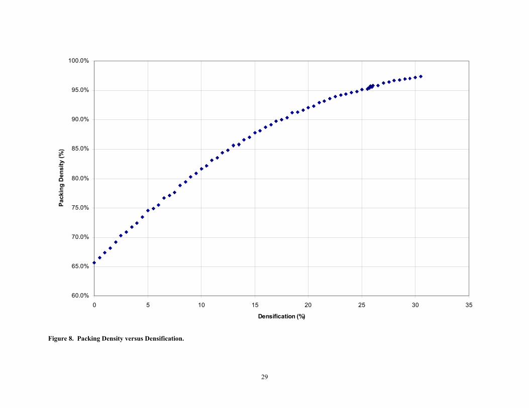
Figure 8 shows the relationship between packing density and densification. As explained
in Section 4.3, densification is simulated by increasing the radii of all particles by the same
percentage, in 0.5% increments. The origin of the plot, at which densification is zero, represents
the initial packing.
Figure 9 shows the solid-void area versus packing density. This graph shows that
decreases with increasing density; however, a slower rate of decrease is expected. In fact, the
computed value of goes to zero at a packing density of about 93%, indicating a problem
with the model in this area. This is discussed further in Section 6.0.
SVVS
SVVS
Figure 10 shows the relationship between the solid-solid surface area and the packing
density. increases steadily with increasing density, then begins to level off at a packing
density of about 95%.
SSVS
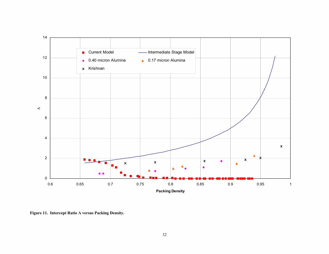
Figure 11and Figure 12 show the model results for the intercept ratio Λ and the surface
area ratio Ψ, respectively, and compare them to results from Krishnan’s model and to
experimental results. The current model shows little agreement with previous models and with
experimental data, except at lower packing densities (below 70%). This is a result of the
behavior of the solid-void surface area, as shown in Figure 9.
28
29
60.0%
65.0%
70.0%
75.0%
80.0%
85.0%
90.0%
95.0%
100.0%
0 5 10 15 20 25 30 35
Densification (%)
Pack
ing
Den
sity
(%)
Figure 8. Packing Density versus Densification.

0
1
2
3
4
5
6
7
0.6 0.65 0.7 0.75 0.8 0.85 0.9 0.95 1
Packing Density
Solid
-Voi
d A
rea
Figure 9. Solid-Void Surface Area versus Packing Density.
30

0
0.5
1
1.5
2
2.5
3
3.5
4
4.5
0.6 0.65 0.7 0.75 0.8 0.85 0.9 0.95 1
Packing Density
Solid
-Sol
id S
urfa
ce A
rea
Figure 10. Solid-Solid Surface Area versus Packing Density.
31
0
2
4
6
8
10
12
14
0.6 0.65 0.7 0.75 0.8 0.85 0.9 0.95 1
Packing Density
Λ
Current Model Intermediate Stage Model
0.40 micron Alumina 0.17 micron Alumina
Krishnan
Figure 11. Intercept Ratio Λ versus Packing Density.
32

0
0.5
1
1.5
2
2.5
3
3.5
4
0.6 0.65 0.7 0.75 0.8 0.85 0.9 0.95 1
Packing Density
Ψ
Current model Intermediate Stage Model
0.40 micron Alumina 0.17 micron Alumina
Krishnan
Figure 12. Surface Area Ratio Ψ versus Packing Density.
33

6.0 DISCUSSION
The current model shows poor agreement with previous models and with experimental
data. This is largely due to problems with the solid-void surface area calculation.
As shown in Figure 9, the solid-void surface area falls off very rapidly, and reaches zero
at a packing density of 93%. Logically, the solid-void surface area would be expected to
decrease linearly, and reach zero at a packing density of 100%. An examination of the model
suggests that the method used to compute the solid-void surface area may be at fault.
The solid-void surface area for each particle is computed as follows. A set of N data
points is generated at random on the surface of the particle. Each point is defined in terms of its
spherical coordinates local to the particle (R, φ, θ) and has an incremental area unit dA
associated with it. The number of points is proportional to the square of the radius; in this case,
10,000R2 points are generated on each particle. Each data point is examined against the
particle’s neighbors. If the data point is not located inside any of the neighboring particles, it
forms part of the solid-void surface. If this is the case, the value of counter j is incremented by
sin θ. Sin θ is used (instead of unity) to ensure that particles at the poles (where sin θ = 0) are not
weighted more heavily than particles at the equator (where sin θ = 1).
Once all data points have been examined, the solid-void surface area for the particle is
calculated:
iii N
jRSV 222π=
34
Where Ri is the radius of the ith particle, and Ni is the total number of data points
examined. The quantities SVi are stored in an array. Once all particles have been considered,
the total solid-void surface area is computed by summing all the values of SVi.
Monte Carlo integration is a technique that requires an exceptionally large number of
data points to converge. It is possible that 10,000R2 data points on the surface of each particle is
insufficient. However, a few trial runs with larger numbers of data points indicate that this is not
the case. In these trials, using 10,000 data points yielded results that were different by less than
10%. Furthermore, using more data points did not, in general, increase the calculated solid-void
surface area; at some densities, the solid-void surface area calculated with more data points was
actually lower.
This fact leads to the conclusion that Monte Carlo integration is not a suitable method for
computing the solid-void surface area, at least for the packing under investigation. A purely
geometric method may need to be employed. This would involve checking the intersection
between the particle under consideration and each of its neighbors, computing the distance
between centers, computing the area of the spherical cap created by the intersection, and
subtracting that surface area from the total surface area of the particle.
The solid-solid surface area increases almost linearly with packing density, and then
begins to level off at a packing density of around 95%. This reduction results from the fact that,
as smaller particles are absorbed by larger ones, the solid-solid surface area computed by the
algorithm is actually smaller than the surface area of the plane through the smaller particle’s
center. See Figure 13. At a packing density of 95%, none of the particles has been completely
35

absorbed by any others. Physically, this is analogous to grain growth, which occurs during final
stage sintering.
Line representing solid-solid surface area.Note that it is shorter than the diameter of thesmaller circle.
Figure 13. Solid-Solid Surface Area Between Two Particles.
36

7.0 CONCLUSIONS
The results from this simulation are disappointing. The problems with the model are
described in the previous section. However, the model presents some positive features. It
generates a close packing, and can be extended to model other sintering conditions.
Once the problems with the calculation of the solid-void surface area have been
addressed, this model may prove valuable in predicting the microstructural properties of a
sintered part based on its geometric properties.
37

8.0 DIRECTIONS FOR FUTURE RESEARCH
The model created for this thesis has many advantages. MATLAB® is a powerful and
easy to use programming language, with many built-in functions and a great deal of flexibility.
Modifying and extending the model is therefore simplified.
Improvements to the model can be made in several areas. First, as noted in Section 6.0,
the method for computing the solid-void surface area needs to be improved. A possible solution
to this problem is outlined in Section 6.0. The particle packing model can also be improved, as
discussed in Section 8.1 below. Finally, different sintering conditions (pressure assisted
sintering, particle movement during sintering, etc.) can be added to the model, as discussed in
Section 8.2 below.
8.1 Refining the Particle Packing Model
Some problems with the particle packing model were identified during its development.
Some difficulty was experienced in getting a close-packed compact when rearranging the
particles. It is believed that a combination of the following modifications may facilitate getting a
close packing:
• Modifying the initial distribution of particle centers,
• Refining the rearrangement geometry (particle movement during rearrangement).
Increasing the number of particles may also assist in getting a close packing. This was
attempted only on a limited basis, as the particle rearrangement algorithm required a lot of
computer time.
38

The current model also fails to take any account of the pore size distribution, which may
play a significant role in the evolution of the microstructure. Zheng and Reed [23] found that
there is a critical ratio of pore size to mean particle size. Pores smaller than this critical ratio
were completely eliminated during sintering, while pores larger than the critical ratio were not.
This is an area that was not explored in the course of this research; however, algorithms for
measuring pore size and pore size distribution exist [31].
8.2 Simulating Different Sintering Conditions
Once a close packing has been achieved, refinements can be made to the densification
part of the model. For instance, a real compact experiences some particle movement during
sintering. This could be integrated into the rearrangement algorithm, by allowing particle
rearrangement between densification steps. Pressure sintering (hydrostatic or isostatic) could
also be simulated. This could be done by allowing particle rearrangement between densification
steps, and imposing a preferred direction of movement, either towards the center of the packing
(for hydrostatic pressure) or downwards (for isostatic pressure). These refinements would
improve the model’s ability to predict microstructural pathways during sintering, and eventually
to help predict the finished shape of a sintered product.
39

APPENDIX A
SIMULATION CODE DESCRIPTION AND ALGORITHMS

The code for the simulation was based on a particle packing routine described by Nolan
and Kavanagh [11, 26]. The algorithms for their routine, which was originally written in Pascal,
were modified and rewritten in MATLAB® for this application.
The simulation proceeds in three stages. In the first stage, an initial packing is generated,
and certain parameters (nearest neighbors, packing density, overlap, etc.) are computed and
stored. The second stage consists of rearranging the packing to minimize overlap and maximize
stability. The third stage consists of expanding (densifying) the packing and computing its
geometric and stereological properties.
Following are verbal descriptions of each section of the code. For sections for which a
verbal description is insufficient, a flowchart showing the algorithm is provided.
Generating the Initial Packing
Generate
This routine generates a random packing of spherical particles. There are NumSpheres
particles, each with a center c and radius r. The particle definitions are stored in a 4 x
NumSpheres array called Particle. Each row of Particle is structured as [x y z r], where x, y and
z are the Cartesian coordinates of the center of the particle, and r is the radius. The spheres are
generated within a unit sphere. A sphere is used (instead of some other shape) because it avoids
edge effects, and because it is isotropic. NumSpheres is entered by the user.
The particles are initially generated around the origin of the unit sphere (that is, particle
centers are normally distributed with 0),,( =zyx ), instead of uniformly throughout the unit
41

sphere. This allows a high initial degree of overlap and contact among the particles, which
allows the packing to be rearranged more effectively. See “Rearranging the Particles” below.
Reduce
The initial packing created by generate places particles randomly in space. Some
particles will be completely inside other particles, and some will be outside the unit sphere
selected as the volume in which the packing is generated. This routine eliminates particles that
are completely inside other particles and particles lying completely outside the unit sphere.
Findlocal
This routine computes an array called touch. The touch array is structured as follows.
Each row represents one particle from the Particle array (i.e., the first row represents the first
particle, the second row represents the second particle, etc.) The number in the first column
indicates how many particles are in contact with that particle. For instance, the number “8” in
the third row indicates that there are eight particles in contact with the third particle in the
Particle array. The numbers in the 2nd through nth columns are the numbers of the contacting
particles. In this example, the third particle is in contact with eight other particles: the first,
fourth, sixth, 10th, 17th, 22nd, 37th, and 62nd. See Figure 14.
The Findlocal routine finds up to 12 particles within one-half the mean particle radius of
each particle.
42

8 1 4 6 10 17 22 37 62 0
Total number of particles in contact with the third particle
The numbers of the contacting particles
Remaining columns are zero
4 3 7 18 29 0 0 0 0 0
Figure 14. Layout of the touch Array.
Density
The Density routine computes the packing density of the particles, as described in
Appendix C. The algorithm for this routine is shown in Figure 21.
Packstat
Packstat computes the packing statistics for the particle arrangement. These statistics
include the separation and/or degree of overlap between adjacent particles, the mean
coordination number of the arrangement, and the fraction of particles that are in a gravitationally
stable configuration. A particle is gravitationally stable if it is supported from underneath by
three other particles.
43

Rearranging the Particles
The packing generated above is not close-packed. The particles are placed in space at
random; many of them overlap, while some are not in contact with any other particles. The
purpose of the rearrangement is to shift the particles around to minimize overlap and maximize
stability. The Rearrange routine loops as long as the mean overlap is more than one-sixth the
mean particle radius, and the fraction of particles in a gravitationally stable configuration is less
than 75%. The algorithm for this routine is given in Figure 19.
Subregion
After the packing is rearranged, most of the particles are clustered around the origin, as
shown in Figure 15. This produces a very low packing density within the unit sphere, as most of
the space in the unit sphere is empty. Therefore, a representative volume, or subregion, of the
original packing is selected. This new subregion has a radius, RegionRadius, equal to the mean
of the particle radii. Most of the particles are located in this subregion. The packing parameters
and touch array are recomputed for the subregion. From this point, only the subregion is
considered. This process eliminates the need to fill a large volume with particles, which would
significantly increase computation time.
44

Figure 15. Location of Particles after Rearrangement.
Solidsolid
The solid-solid surface area between two overlapping spheres is a circle, as shown in
Figure 16. The area of this circle, whose radius is a, is given by πa2, where
222222 )(421 RrdRdd
a +−−= , R and r are the radii of the larger and smaller spheres,
respectively, and d is the distance between the particle centers.
45

Figure 16. Intersection Between Two Spheres.
The situation is more complex when more than two spheres overlap at a point in space.
Physically, this is roughly equivalent to the point at which the necks begin to impinge on each
other. The problem can be illustrated in two dimensions with three overlapping circles. See
Figure 17.
12
3
Segment 1-2
Segment 2-3
Segment 1-3
Figure 17. Intersection of Three Circles.
46

To compute the total contact length among circles 1, 2 and 3 (analogous to the total
contact area among three spheres), one needs to consider parts of line segments 1-2, 1-3 and 2-3:
Figure 18. Total Contact Length for Three Circles.
The dotted line segments in Figure 18 must be removed from the calculation. While this
is simple enough in this example, it becomes very complicated in three dimensions, especially
with more than three particles.
The Geometric Bounding Toolbox (GBT), mentioned elsewhere in this thesis, includes a
routine that computes the contact area of multiple contacting spheres in space. Results from this
routine were compared with results computed geometrically from 2- and 3-particle systems,
which are relatively simple to compute geometrically. The results returned by the GBT were
within 1% of the geometrically calculated results.
Solidvoid
This routine computes the solid-void surface area of the packing, as described in
Appendix C. The algorithm for the solid-void calculation is given in Figure 27 and Figure .
47

Rearrange initial packing
While MeanOverlap > MaxOverlap and
StableCount < MinStable
Contactforce
Overlap => MaxOverlap? Move
Compute Displacement of particle from its original position
Displacement > MinDisplacement? Local Updates touch array after
particle displacement
Particle on outside of packing?
Contactforce
Findstable
Stable = 0 and Outer = 0? Roll
Recompute Displacement
Write particle's new coordinates to Particle array
Packstat Recomputes packing statistics
End rearrangement
YES
NO
YES
NO
YES
NO
NO YES
Figure 19. Algorithm for Rearrange.
48

ContactforceCompute the forces between
a particle and its neighbors
Compute overlap distance between particle and each
neighbor
Compute separation
between particle and neighbor
Examine each neighboring
particle in turn
Particles overlapping? NO
Distance is the overlap distance between a
particle and its neighbor. It is used as the magnitude
of the force vector.
Compute force components Separation
rrForceForce neighborparticle
ii
)( −+=
End
YES
Figure 20. Algorithm for Contactforce.
49

Compute packing density
Generate n=100,000 data points
Array p of 100,000 data points (x, y, z coordinates)
Compute distance of each data point from
center of packing (origin)
Fourth column of p now contains distance from
center
Sort p in order of distance from origin
Points farthest from origin are in first rows of p
While p(i) > RegionRadius
Delete affected row of p
For each particle in
packing
For each data point p(i)
Data point inside particle?
Boolean IN = 0
NO Boolean IN = 1
Counter in = in + 1
PackingDensity = in/n
Recompute n
End
YES
Figure 21. Algorithm for Density.
50

Move particles
Other particles contacting particle?
Set default move distance and
direction (down)NO
Compute move distance based on mean overlap of packing and particle's overlap with neighbors
YES
MoveDistance (ForceComponents from ContactForce calculation)
Compute magnitude of force
vector
MoveDistance, ForceComponents
Compute new coordinates s(i) for
particle tudeForceMagninentsForceCompoceMoveDistan
ss iii
*+=
End
Figure 22. Algorithm for Move.
51

Roll particle around its contacting particles
Define rotation angle based on
mean overlap
Particle in contact with more than one other particle? SingleRotation
Define coordinates and compute
separation from lowest contacting particle a
For each subsequent contacting particle b
Compute separation from contacting
particle b
xa, Separation1
xb, Separation2
Particle b below particle? j = j + 1
j > 0 ? SingleRotation
DoubleRotation
NO
YES
YES
NO
NO
YES
End
Figure 23. Algorithm for Roll.
52
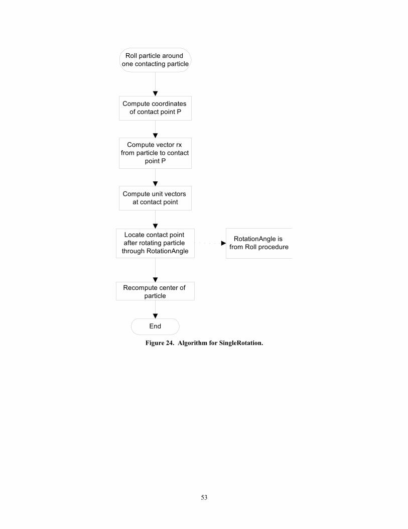
Roll particle around one contacting particle
Compute coordinates of contact point P
Compute vector rx from particle to contact
point P
Compute unit vectors at contact point
Locate contact point after rotating particle
through RotationAngle
RotationAngle is from Roll procedure
Recompute center of particle
End
Figure 24. Algorithm for SingleRotation.
53

Rotate particle around two contacting particles
Compute vectors from particle to contact points
rsxa is the vector to contact point with particle arsxb is the vector to contact point with particle b
Compute the coordinates of the
contact points in the local coordinate system
xa is the coordinate for particle axb is the coordinate for particle b
Compute the distance from particle a to particle
bLength r12
Compute unit vectors at center of rotation
Compute center of rotation Point n
Locate contact point after rotating particle
through RotationAngle
RotationAngle is from Roll procedure
Recompute center of particle
End
Figure 25. Algorithm for DoubleRotation.
54

Determine whether a particle is in a stable
configuration A particle is in a stable configuration if it is supported
by three other particlesInitialize boolean
variable Stable = 0
Create array of coordinates of three
neighborsTriad
Compute coordinates of plane passing
through centers of particles in Triad
m
Compute angles of lines from centers of particles in Triad to
center of particle
Angles form a stable base? Stable = 0NO
Stable = 1
YES
Identify particle's three neighbors
Stable = 1 ?NO
End
If there are more than three contacting particles, each group of
three neighbors is considered in turn
YES
Figure 26. Algorithm for Findstable.
55

Compute the solid-void surface area
For each particle SphereNumber
Define parameters of particle
Initialize counter j
Particle touching any other particles?
Entire surface of particle is part of solid-void surface
SV(SphereNumber) = Entire surface areaNO
Go to page 2
Back from
page 2
njrerSphereNumbSV
222)( π=
SVArea = sum of all terms in SV array
End
YES
Figure 27. Algorithm for Solid-Void Calculation.
56

Generate n data points on the surface of the particle
For each data point i
Convert coordinates to global Cartesian coordinate system
For each contacting particle k in the touch
array
Data point i inside particle k?
Area unit associated with data point i cannot be
part of solid-void surfaceYES
Boolean variable SURF = 1
Boolean variable SURF = 0
SURF = 1 ?NO
Local spherical coordinates are R, phi and theta; global Cartesian
coordinates are x, y and z.
From page 1
This data point is not part of the S-V surface, so there is no point in checking it against the
other contacting particles
j = j + sin(theta)
Back to page 1
YES
NO
Does i lie within subregion?
YES
NO
Figure 27 (continued). Algorithm for Solid-Void Calculation.
57

APPENDIX B
THE LOG-NORMAL DISTRIBUTION

Many researchers consider that the log-normal distribution best represents the true
particle size distribution [12, 13]. The log-normal distribution is a continuous distribution in
which the logarithm of a variable x is normally distributed [22]. It is described by
2
2))(ln(
2
21)( σ
µ
πσ
−−
=x
ex
xP
Where µ is the mean of the underlying normal distribution, and σ2 is the variance of the
underlying normal distribution. The mean and variance of the log-normal distribution are given
by
2ln
2σµµ += e
and
)1(22 2
ln −= + σµσσ ee
An example of the log-normal distribution is shown in Figure 28.
59

Figure 28. The Log-Normal Distribution.
The log-normal distribution is skewed to the left relative to a normal distribution with the
same underlying mean and variance.
60

APPENDIX C
MONTE CARLO INTEGRATION

C-1 Background
Monte Carlo integration is a numerical integration technique that can be used to estimate
the value of an integral when an analytical solution cannot be found [32]. Consider the integral
as representing the area under the curve g(x) from a to b as shown in Figure 29. Ω
denotes the rectangle defined by a, b and c, as shown.
∫=b
adxxgI )(
y
x
x "HIT"
x "MISS"
Ω
g(x)
a b
c
Figure 29. Monte Carlo Integration.
Let (X,Y) be a random vector uniformly distributed over the rectangle Ω with probability
density function
Ω∈
−=otherwise
yxifabcyxf XY
0
),()(
1),(
The probability p that (X,Y) falls within the area under the curve g(x) can be written as
62

)()(
)()(abc
Iabc
dxxg
ofareaxgcurveunderarea
p
b
a
−=
−=
Ω=
∫
If N independent random vectors (X1,Y1), (X2, Y2), …, (XN, YN) are generated, the
probability p can be estimated by
NN
p H=ˆ
Where NH is the number of times ; that is, the number of “hits,” as shown in
Figure 29. From these two equations, we can estimate the value of the integral I as
ii YXg ≥)(
NN
abcI H)( −≅ .
In other words, the value of the integral I is the fraction of points that lie under the curve
defined by g(x) multiplied by the area of the rectangle Ω.
This thesis uses Monte Carlo integration to estimate two quantities: the packing density
and the solid-void surface area.
C-2 Estimation of Packing Density
For a non-overlapping packing, the packing density can be computed exactly by adding
up the volumes of all the particles and dividing this quantity by the volume of the region:
31
3
)(Re34
gionRadius
rsityPackingDen
N
ii∑
== π .
63

However, once the packing has been expanded, neighboring particles will overlap. Using
the simple geometric technique just described will result in packing densities greater than unity,
which are physically impossible. Once the packing has been expanded, the overlapping volume
fractions of adjacent particles need to be taken out of the calculation (see Figure 30). This
proved to be extremely difficult, so Monte Carlo integration was used to estimate the volumes of
the particles.
Part of each shaded area must be removed.
Figure 30. Overlapping Volume Fractions in the Density Calculation.
A uniform random sample of N data points is generated in the interval (-RegionRadius,
RegionRadius). This region represents a cube of side 2*RegionRadius. All data points in the
sample that were outside the spherical region of radius RegionRadius were removed from the
sample, leaving a uniform random sample of data points in the spherical region of interest. See
Figure 31.
64

Figure 31. Cube with Inscribed Sphere.
The program considers each data point Ni in turn, checking whether it is inside the first
particle in the Particles array (the Geometric Bounding Toolbox, described elsewhere in this
thesis, includes a routine for doing this). If it is not, the program checks it against the next
particle, and so on, until the point is inside a particle, or until it has been checked against all
particles. The next data point is then considered, and so on, until all N points have been
considered.
If the data point Ni is inside a particle, the Boolean variable IN is assigned a value of 1,
the counter in* is incremented by one and the program moves on to the next data point. If the
data point Ni is not inside any of the particles, the Boolean variable IN is assigned a value of 0.
Once all N data points have been checked against all particles, the packing density is
estimated by NinsityPackingDen = . The algorithm for this routine is given in Figure 21.
This method was checked against the purely geometric method for several non-
overlapping packings. It was found that an initial value of N = 100,000 data points produced a
* Variable names in MATLAB® are case-sensitive; IN, in and In are all different variables.
65
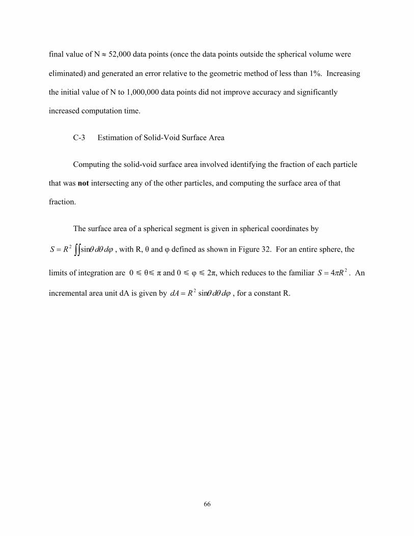
final value of N ≈ 52,000 data points (once the data points outside the spherical volume were
eliminated) and generated an error relative to the geometric method of less than 1%. Increasing
the initial value of N to 1,000,000 data points did not improve accuracy and significantly
increased computation time.
C-3 Estimation of Solid-Void Surface Area
Computing the solid-void surface area involved identifying the fraction of each particle
that was not intersecting any of the other particles, and computing the surface area of that
fraction.
The surface area of a spherical segment is given in spherical coordinates by
, with R, θ and φ defined as shown in Figure 32. For an entire sphere, the
limits of integration are 0 θ π and 0 φ 2π, which reduces to the familiar . An
incremental area unit dA is given by , for a constant R.
∫∫= ϕθθ ddRS sin2
24 RS π=
ϕθθ ddRdA sin2=
66

Rsinθdφ
Rdθ
R
y
x
z
φ
θ
Incremental area dA
Figure 32. Incremental Area in Spherical Coordinates.
A uniformly distributed random sample of points Ni is generated on the surface of the ith
particle. These are generated in spherical coordinates (R,φ,θ) local to the particle. The
coordinates of each point are transformed into Cartesian coordinates (x’,y’,z’) local to the
particle, and then into global Cartesian coordinates (x, y, z) (see Figure 33). The conversion
from spherical to Cartesian coordinates is given by
cosφsinθRx = sinθinθsRy =
θcosRz =
67
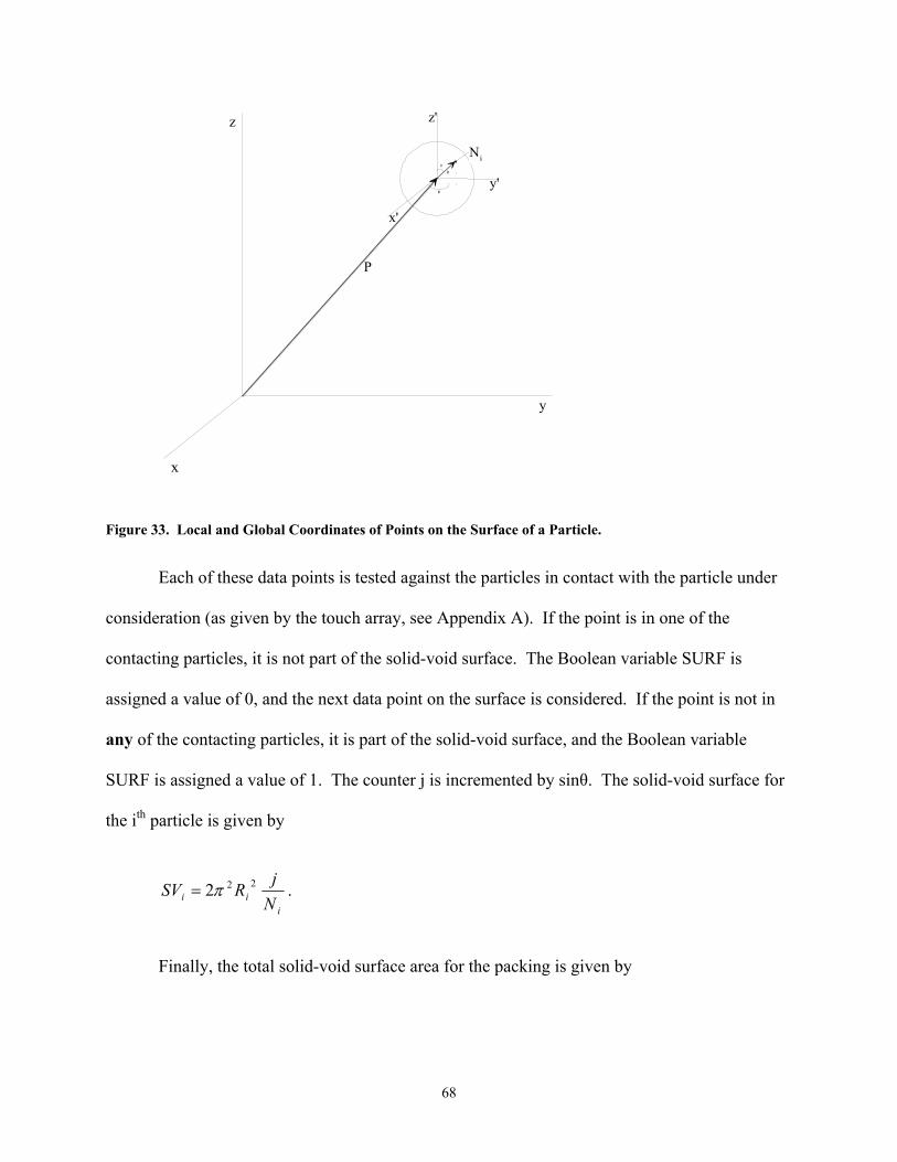
y
x
z
x'
y'
z'
R
φ
θ
Ni
P
Figure 33. Local and Global Coordinates of Points on the Surface of a Particle.
Each of these data points is tested against the particles in contact with the particle under
consideration (as given by the touch array, see Appendix A). If the point is in one of the
contacting particles, it is not part of the solid-void surface. The Boolean variable SURF is
assigned a value of 0, and the next data point on the surface is considered. If the point is not in
any of the contacting particles, it is part of the solid-void surface, and the Boolean variable
SURF is assigned a value of 1. The counter j is incremented by sinθ. The solid-void surface for
the ith particle is given by
iii N
jRSV 222π= .
Finally, the total solid-void surface area for the packing is given by
68

∑=
=n
kkSVSVArea
1.
The algorithm for the solid-void calculation is given in Figure 27.
This method was checked against a geometric solid-void surface area calculation for
various one- and two-particle models. It was found that values of generated an
error relative to the geometric method of less than 2%. However, the solid-void surface area
became zero at less than 100% densification. Using more data points might overcome or
mitigate this problem.
2000,100 ii RN ∝
69

BIBLIOGRAPHY
BIBLIOGRAPHY
1. German, R.M., Sintering Theory and Practice. 1996, New York: John Wiley and Sons.
2. Ashby, M.F., A first report on sintering diagrams. Acta Metallurgica, 1974. 22: p. 275-289.
3. Aigeltinger, E.H. and R.T. DeHoff, Quantitative determination of topological and metric properties during sintering of copper. Metallurgical Transactions A, 1975. 6A: p. 1853-1862.
4. Kingery, W.D., H.K. Bowden, and D.R. Uhlmann, Introduction to Ceramics. Second ed. Wiley Series on the Science and Technology of Materials. 1976, New York: John Wiley & Sons. 1032.
5. Exner, H.E. and E. Arzt, Sintering Processes, in Physical Metallurgy, R.W. Cahn and P. Haasen, Editors. 1996, Elsevier Science: Amsterdam. p. 2628-2662.
6. Slaughter, W.S., et al., A quantitative analysis of the effect of geometric assumptions in sintering models. Acta Metallurgica, 1997. 45(12): p. 5077-5086.
7. Baddeley, A., Stereology, in Spatial Statistics and Digital Image Analysis. 1991, National Academy Press: Washington, D.C.
8. DeHoff, R.T. and F.N. Rhines, Quantitative Microscopy. 1968: McGraw-Hill.
9. Smith, L.N. and P.S. Midha, Computer simulation of morphology and packing behaviour of irregular particles, for predicting apparent powder densities. Computational Materials Science, 1997. 7: p. 377-383.
10. Nankadumar, K., Y. Shu, and K.T. Chuang, Predicting geometrical properties of random packed beds from computer simulation. AIChE Journal, 1999. 45(11): p. 2286-2297.
11. Nolan, G.T. and P.E. Kavanagh, Computer simulation of random packing of hard spheres. Powder Technology, 1992. 72: p. 149-155.
12. Patterson, B.R. and J.A. Griffin. Effect of particle size distribution on sintering of tungsten. in International Powder Metallurgy Conference. 1984. Toronto, Ontario: Metal Powder Industries Federation.
13. Patterson, B.R. and V.D. Parkhe. Particle size distribution effects on sintering of spherical tungsten. in Annual Powder Metallurgy Conference. 1985. San Francisco: Metal Powder Industries Federation.
71

72
14. Shiau, F.-S., T.-T. Fang, and T.-H. Leu, Effects of milling and particle size distribution on the sintering behavior and the evolution of the microstructure in sintering powder compacts. Materials Chemistry and Physics, 1998. 57: p. 33-40.
15. Yeh, T.-S. and M.D. Sacks, Effect of particle size distribution on the sintering of alumina. Journal of the American Ceramic Society, 1988. 71(12): p. C484-C487.
16. Ting, J.-M. and R.Y. Lin, Effect of particle-size distribution on sintering Part I Modeling. Journal of Materials Science, 1994. 29: p. 1867-1872.
17. Ting, J.-M. and R.Y. Lin, Effect of particle size distribution on sintering Part II Sintering of alumina. Journal of Materials Science, 1995. 30: p. 2382-2389.
18. Matheson, A.J., Computation of a random packing of hard spheres. Journal of Physics C: Solid State Physics, 1974. 7: p. 2569-2576.
19. Smith, L.N. and P.S. Midha, A computer model for relating powder density to composition, employing simulations of dense random packings of monosized and bimodal spherical particles. Journal of Materials Processing Technology, 1997. 72: p. 277-282.
20. Milne, S.J., M. Patel, and E. Dickinson, Experimental studies of particle packing and sintering behaviour of monosize and bimodal spherical silica powders. Journal of the European Ceramic Society, 1993. 11(1): p. 1-7.
21. German, R.M., Powder Metallurgy Science. 1984, Princeton: Metal Powder Industries Federation.
22. Weisstein, E., Log Normal Distribution. 1999, Wolfram Research.
23. Zheng, J. and J.S. Reed, Effects of particle packing characteristics on solid-state sintering. Journal of the American Ceramic Society, 1989. 72(5): p. 810-817.
24. Edwards, S.F., Equations of granular materials. Physica A, 1999. 274: p. 310-319.
25. Krishnan, K., Modeling Sintering in Ceramics, in Mechanical Engineering. 2000, University of Pittsburgh: Pittsburgh. p. 130.
26. Nolan, G.T. and P.E. Kavanagh, Computer simulation of random packings of spheres with log-normal distributions. Powder Technology, 1993. 76: p. 309-316.
27. Exner, H.E., Principles of Single Phase Sintering, in Reviews in Powder Metallurgy and Physical Ceramics. 1979. p. 7-251.
28. Nettleship, I., et al. Dimensionless parameters for the analysis of sintering microstructures. in International Conference on Powder Metallurgy and Particulate Materials. 1997. Chicago: Metal Powder Industries Federation.
29. Nettleship, I. and W.S. Slaughter, Dimensionless parameters for microstructural pathways in sintering. Journal of the American Ceramic Society, 1998. 81(3): p. 700-704.
30. Veres, S.M. and D.Q. Mayne, Geometric Bounding Toolbox, Version 7.2. 2002.
31. Nolan, G.T. and P.E. Kavanagh, The size distribution of interstices in random packings of spheres. Powder Technology, 1994. 78: p. 231-238.
32. Rubinstein, R.Y., Simulation and the Monte Carlo Method. Wiley series in probability and mathematical statistics. 1981, New York: John Wiley and Sons.