Computer Labs for MTH U343 Spring 2004 Textbook ... · Computer Labs for MTH U343 Spring 2004 Textbook: DiﬀerentialEquations and Linear Algebra by Edwards & Penney Contents Lab

Computer Labs for MTH U343

Spring 2004

Textbook: Differential Equations and Linear Algebra

by Edwards & Penney

Contents

Lab 1: Slope Fields and Solution Curves

Lab 2: Numerical Methods of Euler

Lab 3: The Runge-Kutta Method

Lab 4: Numerical Methods for Systems

Lab 5: MATLAB and 2nd-order Differential Equations

Computer Lab 1: Slope Fields and Solution Curves

The equation y′ = f(x, y) determines a slope field (or direction field) in the xy-plane:the value f(x, y) is the slope of a tiny line segment at the point (x, y). It has geometricalsignificance for solution curves which are simply graphs of solutions y(x) of the equation:at each point (x0, y0) on a solution curve, f(x0, y0) is the slope of the tangent line to thecurve. If we sketch the slope field, and then try to draw curves which are tangent to thisfield at each point, we get a good idea how the various solutions behave. In particular,if we pick (x0, y0) and try to draw a curve passing through (x0, y0) which is everywheretangent to the slope field, we should get the graph of the solution of the initial-valueproblem y′ = f(x, y), y(x0) = y0.

I. SKETCHING BY COMPUTER. The sketching of the slope field is tedious by hand,and is expedited by using a computer; the appropriate software will also enable us to plotsolution curves. One such program called “Diffs” uses MATLAB for its computations, andis available on most of the computers in the Math Dept Computer Lab, 553 Lake Hall.(We shall encounter MATLAB more directly in Lab 5, but no knowledge of MATLABis requred for this Lab.) To access Diffs, open up MATLAB; then enter “diffs” at theMATLAB prompt >>.

Diffs is fairly self-explanatory, and assistance is available from the lab mentors, butwe shall illustrate its operation with an example.

Example 1. y′ = y2 − yx.1. After “y′ = f(x, y) =”, type “yˆ2 − y ∗ x”. (Quotation marks not part of input.)2. After “x min=”, type “0”, and after “x max=”, type “4”; this tells MATLAB to

use 0 ≤ x ≤ 4 for plotting purposes. Similarly, enter y min = −1 and y max = 4 toget the plotting range −1 ≤ y ≤ 4. Then click on DRAW, and the screen displaysa sketch of the direction field in the rectangle 0 ≤ x ≤ 4, −1 ≤ y ≤ 4.

3. Select an initial value (x0, y0) for your solution in one of two ways:i) enter the values for x0 and y0, and then click Sketch; orii) use the mouse to move the cursor to select an initial value, and then click to

sketch the solution curve.For example, select (x0, y0) = (0, 1) and sketch the solution curve.

4. Sketch as many solution curves as you need to see the “phase portrait” of yourequation. In particular, you will be able to see “rivers,” which are places wheresolution curves concentrate so as to become indistinguishable on the screen.

Exercise 1. y′ = y − x2

(a) Use Diffs to plot the slope field for −3 ≤ x ≤ 3, −1 ≤ y ≤ 4.(b) Notice that at some points (x, y) there are horizontal tangents, i.e. y′ = 0. Ap-

proximate some of these points using the cross hairs. Can you find exactly the curveof points where y′ = 0? (This is the 0-isocline for the equation.)

(c) Consider the initial condition y(0) = 0. From looking at the slope field near (0, 0),what do you expect the solution curve to do as x increases? Check this by selectingan initial condition very close to (0, 0) and plotting the solution curve.

1

2 Computer Labs for MTH U343

(d) Choose many more initial conditions until you see the phase portrait and therivers.

(e) Now consider the initial condition y(0) = 1.5. From looking at the slope field near(0, 1.5), what do you expect the solution curve to do as x increases? Check this byplotting a solution curve. (You may want to increase the x, y range to somethinglike −3 ≤ x ≤ 5.)

HAND IN: Written answers to the questions in parts (b), (c), and (e). (In (b),for example, “The curve of points where y′ = 0 is . . . ”.) You may also hand inprint-outs of your plots, but your written answers are the most important thing.

II. ASYMPTOTIC BEHAVIOR. Example 1 and Exercise 1 raise an interesting issue:what happens to a solution y(x) of an initial value problem y′ = f(x, y), y(x0) = y0 as xincreases? For example, y′ = y, y(0) = y0 has the solution y(x) = y0e

x which is definedfor all values x (although y(x) → ∞ as x → ∞). On the other hand, for another equationit may be that a solution y(x) escapes to infinity or blows up in that y(x) → ±∞ as xincreases to some finite value x1.

Example 2. y′ = y2. If we use Diffs to plot the slope field, we cannot tell if a solution curveescapes to infinity or not. For example, with the initial condition y(0) = 1, the solutioncurve looks somewhat like exponential growth, but it may actually grow so rapidly thatthe solution reaches +∞ at a finite value of x. To settle the question, notice that theequation is separable and so is easily solved:

dy

dx= y2 ⇒

∫dy

y2=

∫dx ⇒ −1

y= x+ C.

The initial condition y(0) = 1 determines C = −1, so the solution is y(x) = 1/(1−x). Wesee that indeed the solution blows up at x = 1: y(x) → +∞ as x → 1.

On the other hand, not all solutions of the equation blow up. In fact, with initialcondition y(x0) = 0 we have the trivial solution y(x) ≡ 0. This solution appears in theslope field as the horizontal solution curve along the x-axis.

Example 2 has also illustrated a special kind of solution when the equation is au-tonomous, i.e. the function f depends on y but not on x: y′ = f(y). Values of y for whichf(y) = 0 are called critical points. If y = c is a critical point, then the constant functiony(x) ≡ c defines an equilibrium solution whose solution curve is just the horizontal straightline y = c in the xy-plane. In Example 2, y(x) ≡ 0 is an equilibrium solution. But noticethat if we take y0 very close to zero, then the solution with initial condition y(x0) = y0

does not remain close to the equilibrium solution, but in fact escapes to infinity at somex1 > x0. Such equilibrium solutions are called unstable. On the other hand, if all solutioncurves which begin near an equilibrium solution y(x) ≡ c remain near the equilibrium, thenthe equilibrium is call stable; in fact, if all nearby solution curves satisfy limx→∞ y(x) = c,then the equilibrium is called asymptotically stable.

Exercise 2. y′ = y(y − 2)(a) Use Diffs to plot the slope field for 0 ≤ x ≤ 4, −2 ≤ y ≤ 4.

Lab 1: Slope Fields and Solution Curves 3

(b) Notice that the equation is autonomous; what are the equilibrium solutions of theequation? Determine if each one is unstable or asymptotically stable.

(c) If we take the initial condition y(0) = 1, what happens to y(x) as x increases?Does y(x) escape to infinity? Is there a limit of y as x → ∞?

(d) If we take the initial condition y(0) = 3, what happens to y(x) as x increases?Can you show that y(x) escapes to infinity? Hint: The equation is separable, andleads to an integration by partial fractions.

HAND IN: Written answers to the questions in parts (b), (c), and (d). ( In (b), forexample, “There is an equilibrium point at . . .which is . . . (unstable or asymptoti-cally stable). There is also an equilibrium at . . . ”)

III. UNIQUENESS. Notice that the solution of the initial value problem

(IV P )

dy

dx=f(x, y)

y(x0) = y0

may escape to infinity, but it should exist at least near the point (x0, y0), provided f(x, y)is continuous at (x0, y0). Indeed, this is guaranteed by the fundamental Existence andUniqueness Theorem on page 23 of the Edwards and Penney textbook. Notice thatuniqueness of the solution requires ∂f/∂y to be continuous near (x0, y0): if ∂f/∂y isnot continuous at (x0, y0), then uniqueness may fail.

Exercise 3. y′ = y2/3

(a) Use Diffs to plot the slope field on 0 ≤ x ≤ 4, −1 ≤ y ≤ 8.(b) Use Diffs to sketch the solution curve for the initial condition y(0) = y0 withy0 > 0 as close to zero as you can get. (Note: do not use y0 < 0, because theprogram will have trouble evaluating it.) The result should suggest that the initialvalue problem y′ = y2/3, y(0) = 0 has a solution with y(x) → ∞ as x → x1, wherex1 is either a finite value or possibly x1 = ∞. Use separation of variables to findthe solution and the value of x1.

(c) Observe that y(x) ≡ 0 is also a solution of y′ = y2/3, y(0) = 0. Thus uniquenessfails. Would you expect uniqueness to hold for the problem y′ = y2/3, y(0) = 1?

HAND IN: Written answers to the questions in parts (b) and (c).

Lab 2: Numerical Methods of Euler

A numerical method for approximating the solution of the initial-value problem

(∗){y′ =f(x, y)y(a) = y0

involves replacing the continuous variable x by a set of discrete values x0 = a, x1 =x0 + h, x2 = x1 + h = x0 + 2h, . . . with uniform step size h. The goal is to producesuitable approximations y1, y2, . . . to the true values y(x1), y(x2), . . . of the solution y(x)evaluated at the points x1, x2, . . .. Usually, the approximations y1, y2, . . . are defined usingan iteration scheme: assuming we have found y1, y2, . . . , yn, what is the recipe for findingyn+1? Since we are given y0 in the initial condition, we can find y1, and then using y0 andy1 we find y2, etc. The different numerical methods discussed below all follow this pattern,and only differ in the particular iteration scheme. (Any one method may be made moreaccurate by decreasing the step size h.)

I. EULER’S METHOD. The idea of this method is to approximate the curve y(x) on[xn, xn+1] by a straight line with slope s = ∆y/∆x = (yn+1 − yn)/h = f(xn, yn). Solvingfor yn+1 we obtain the simple iteration scheme

(E) yn+1 = yn + hf(xn, yn).

Computing the values y1, y2, . . . can be time-consuming by hand, but is a simple task fora computer. One can write a simple computer program (say in PASCAL or BASIC) tocompute the sequence y1, y2, . . ., but we shall carry out the iteration on a spreadsheetprogram such as EXCEL, which is available on all the machines in the Math computer labin 553 LA. (On PCs running Windows NT, use the Start button and look under NUNetApplications (Installed Locally) for Microsoft Office. On Macs, there is an MS Office folderon the hard disk.) Spreadsheets have the advantage of giving a clear visual display of theprocedure, as well as a graphical representation of the outcome.

Let us discuss a simple example.

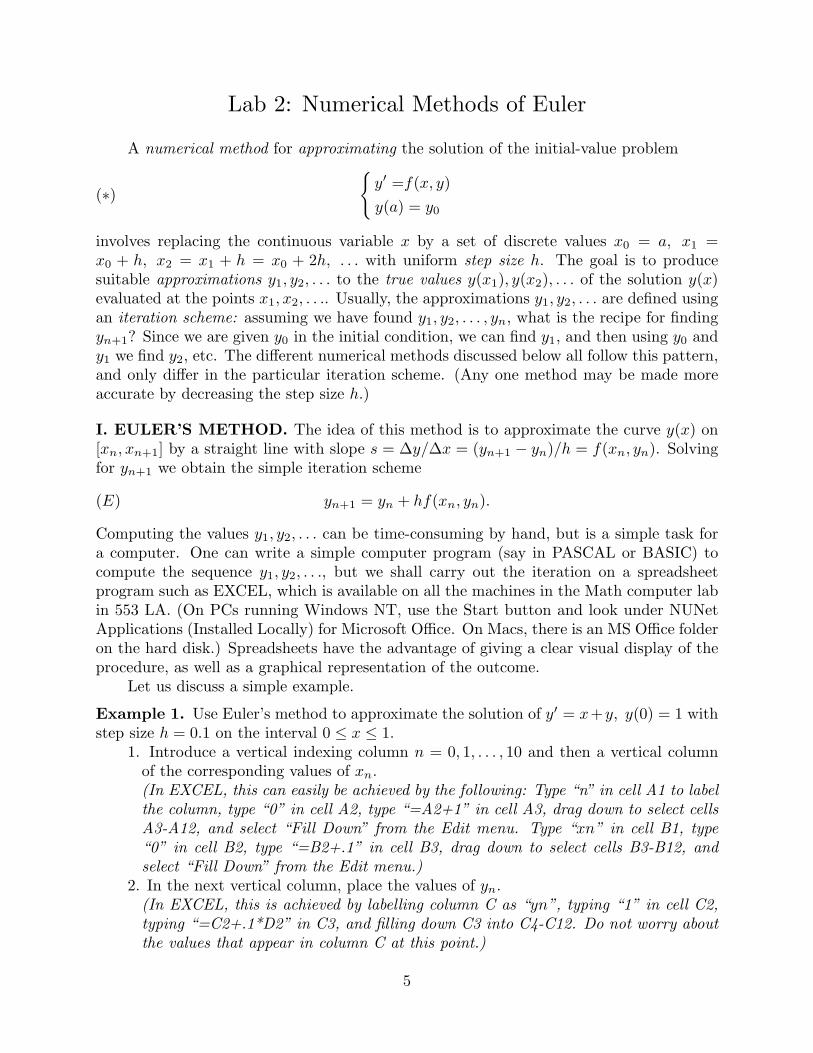
Example 1. Use Euler’s method to approximate the solution of y′ = x+y, y(0) = 1 withstep size h = 0.1 on the interval 0 ≤ x ≤ 1.

1. Introduce a vertical indexing column n = 0, 1, . . . , 10 and then a vertical columnof the corresponding values of xn.(In EXCEL, this can easily be achieved by the following: Type “n” in cell A1 to labelthe column, type “0” in cell A2, type “=A2+1” in cell A3, drag down to select cellsA3-A12, and select “Fill Down” from the Edit menu. Type “xn” in cell B1, type“0” in cell B2, type “=B2+.1” in cell B3, drag down to select cells B3-B12, andselect “Fill Down” from the Edit menu.)

2. In the next vertical column, place the values of yn.(In EXCEL, this is achieved by labelling column C as “yn”, typing “1” in cell C2,typing “=C2+.1*D2” in C3, and filling down C3 into C4-C12. Do not worry aboutthe values that appear in column C at this point.)

5

Euler's Method

x n

yn

01234

0

0.1

0.2

0.3

0.4

0.5

0.6

0.7

0.8

0.9 1


3. In the next vertical column, place the values of the slopes sn = f(xn, yn).(In EXCEL, this is achieved by labelling column D as “sn = f(xn, yn)”, typing“=B2+C2” in cell D2, and filling down D2 into D3-D12: notice that this affects theC column as well.)

4. Now that the approximations y1, . . . , y10 have been found, they may be graphedversus x1, . . . , x10. The result should approximate the graph of the actual solutiony(x).(In EXCEL, this is achieved by dragging the cursor over the xn and yn values toselect these columns, then clicking on the Chart Wizard icon which has a pictureof a chart and a magic wand, and should be second from the right on the controlbar above your worksheet. Next use the mouse to select a rectangular section ofyour worksheet where the graph will appear. A series of dialogue boxes will set theparameters. Step 1: check the variable range; if OK click on “Next”. Step 2: selectLine as chart type; click on “Next”. Step 3: select 1 as the format; click on “Next”.Step 4: be sure “Use first column for:” has “Category X Axis Labels” selected; click“Next”. Step 5. you do not need a legend at this point, but you could entitle thechart “Euler’s Method” and the X axis “xn” and the Y axis “yn”.)The result looks like the following:

To investigate the accuracy of Euler’s method, let us compare the approximationsy1, y2, . . . with the actual solution values y(x1), y(x2), . . .. Of course, if we can actuallysolve (*), then we do not even need a numerical method. But for experimental purposes,let us consider a linear equation y′ + P (x)y = Q(x) for which the solution is given inthe text (Edwards & Penney, Section 1.5). In particular, for the initial value problem ofExample 1, y′ = x+ y, y(0) = 1, we find the solution is y(x) = 2ex − x− 1.

Example 1 (cont’d). Compare the approximations y1, . . . , y10 with the actual valuesy(x1), . . . , y(x10).

5. Create column E for the values y(xn).(In EXCEL, use the formula “= 2∗exp(B2)−B2−1” in cell E2, and then fill downinto E3-E12.)

6. Create column F for the difference y(xn) − yn.

Lab 2: Numerical Methods of Euler 7

(In EXCEL, use the formula “= E2 − C2” in cell F2, and then fill down intoF3-F12.)

Your spreadsheet should now look like the following:

n xn yn sn = f(xn, yn) y(xn) y(xn) − yn0 0 1 1 1 01 0.1 1.1 1.2 1.110342 0.0103422 0.2 1.22 1.42 1.242806 0.0228063 0.3 1.362 1.662 1.399718 0.0377184 0.4 1.5282 1.9282 1.583649 0.0554495 0.5 1.72102 2.22102 1.797443 0.0764236 0.6 1.943122 2.543122 2.044238 0.1011167 0.7 2.197434 2.897434 2.327505 0.1300718 0.8 2.487178 3.287178 2.651082 0.1639049 0.9 2.815895 3.715895 3.019206 0.20331110 1 3.187485 4.187485 3.436564 0.249079

Notice that the differences y(xn) − yn get larger as n increases; in other words, theaccuracy of the approximations gets worse as we get further away from the initial value(a, y0).

Exercise 1. Consider the initial-value problem y′ − 2y = 3e2x, y(0) = 0.(a) Use Euler’s method with step size h = .1 on the interval 0 ≤ x ≤ 2 to find

the approximations y1, . . . , y20. What is the approximation for y(2) that you haveobtained?

(b) Find the actual solution y(x) using Section 1.5 in the text. What is the actualvalue y(2)?

(c) Use Euler’s method with step size h = .05 on the interval 0 ≤ x ≤ 2 to find approx-imations y1, . . . , y40. What is the approximation for y(2) that you have obtained?

(d) Which of the approximations (a) or (c) is closer to the actual value (b)? Howcould you improve the approximation even more?

Hand In: A print-out of your EXCEL worksheet and your answers to all five of thequestions asked in (a-d). (Be very complete in your answer to the last question.)

II. IMPROVED EULER’S METHOD. As we have seen, inaccuracies in Euler’smethod develop quickly with successive steps. This is partly due to the asymmetry inusing the slope at xn to approximate yn+1 without taking into account the slope at xn+1.Consider, instead, the following iteration scheme:

(E∗)yn+1 = yn + h(k1 + k2)/2k1 = f(xn, yn)k2 = f(xn+1, yn + hk1).

Notice that k1, which we formerly called sn, is the slope at the starting point (xn, yn),and k2 is the slope at the point (xn+1, yn + hk1) which the Euler method produced. The


improved Euler method (E∗) uses the average of these two slopes to produce the new valueyn+1.

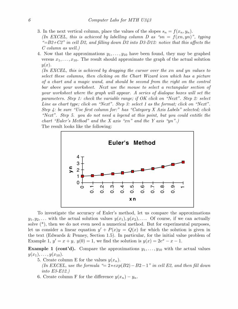
If we use EXCEL to perform the improved Euler method on the problem of Example1, we obtain the following display:

n xn yn k1 k2 y(xn) y(xn) − yn0 0 1 1 1.2 1 01 0.1 1.11 1.21 1.431 1.110342 0.0003422 0.2 1.24205 1.44205 1.686255 1.242806 0.0007563 0.3 1.398465 1.698465 1.968312 1.399718 0.0012524 0.4 1.581804 1.981804 2.279985 1.583649 0.0018455 0.5 1.794894 2.294894 2.624383 1.797443 0.0025496 0.6 2.040857 2.640857 3.004943 2.044238 0.0033807 0.7 2.323147 3.023147 3.425462 2.327505 0.0043588 0.8 2.645578 3.445578 3.890136 2.651082 0.0055049 0.9 3.012364 3.912364 4.40360 3.019206 0.00684310 1 3.428162 4.428162 3.870978 3.436564 0.008402

where, as before, yn are the approximations, and y(xn) are the exact values. (Notice thatthe value of k2 in the last line is suspicious, since it decreased from the previous line. Thisis because the formula for the nth line of k2 requires the value xn+1 which does not existfor n = 10; so EXCEL assigns the default value 0, making this value for k2 incorrect!However, this value for k2 is irrelevant for the other values in the table (do you see why?).

The last column shows the accuracy of the method. Notice that the improved Eulermethod is indeed much more accurate than the ordinary Euler method; however, even herethe method becomes less accurate with successive steps.

Exercise 2. Use the improved Euler method with step size h = .1 on the interval 0 ≤ x ≤ 2to find numerical approximations for the same problem as in Exercise 1. Graph the valuesyn versus xn, and compute the accuracy y(xn)− yn. Are these results more accurate thanthose of Excerise 1?

Hand In: A print-out of your EXCEL worksheet showing the values of xn, yn, k1,k2, y(xn), and y(xn) − yn, and the graph of yn versus xn; also a complete-sentenceanswer to the question.

III. ERROR ESTIMATES. As we have seen with both the Euler method (E) and theimproved Euler method (E∗), errors creep in at each step and accumulate with successivesteps to limit the accuracy of the numerical values. The error at each step is called thelocal error, and the accumulated error at the last step is called the global or cumulativeerror. For a given step size h, we would like to estimate these errors.

The local error, e(h), is easy to estimate using Taylor’s formula with remainder:

y(x) = y(a) + y′(a) (x− a) +12y′′(c) (x− a)2 where c lies between x and a.

Assuming y(xn) = yn is accurate, let a = xn, x = xn+1, h = xn+1 − xn, and y′(a) =


y′(xn) = f(xn, yn) to obtain

y(xn+1) = y(xn) + f(xn, yn)h+12y′′(c)h2.

Comparing this with (E), we see that the local error e(h) = |y(xn+1) − yn+1| for Euler’smethod is given by

e(h) ≤ Mh2, where M =12

max{|y′′(c)| : xn ≤ c ≤ xn+1}.

Of course, we have no idea how big M is, since it depends on y′′(x) which we do not knowin practice. But, as an estimate of how the accuracy depends on the step size h, this meansthat the local error goes to zero like h2, as h → 0. This is sometimes written as

e(h) = O(h2) as h → 0.

The global error, E(h), is of course more important than the local error since itmeasures the accuracy of our final numerical answer, say at x = b where b > a. Of course,it is more complicated to estimate, because the local error at each step can be different.One way around this is to assume the constant M above works for every n:

M =12

max{|y′′(x)| : a ≤ x ≤ b}.

The number of steps N is related to the step size h by N = Lh−1, where L = b− a is thetotal length of the x-values. (In Example 1, L = 1 and N = 10.) Since the local errorsaccumulate N times, we find that

E(h) ≤ Ne(h) = Lh−1e(h) ≤ Lh−1Mh2 = LMh;

without trying to compute M , we can at least conclude that

E(h) = O(h) as h → 0.

This is expressed by saying that Euler’s method is a first-order method.Let us illustrate this error analysis with our example.

Example 1 (cont’d). Compare the local error and global error for various step sizes inthe Euler approximations for the solution of y′ = x+ y, y(0) = 1, taking N = 10, N = 20,N = 30, N = 40, and N = 50. Based on these, what errors would you expect for N = 100?

1. We have already taken N = 10 (h = .1), so let us take N = 20 (h = .05).(Increase the length of the “n” column to end with n = 20. Then revise the “xn”column to reflect xn+1 = xn + .05, and the “yn” column to reflect yn+1 = yn +.05f(xn, yn); in both cases, you may change the first entry, and then “fill down”.We shall also need to “fill down” the three remaining columns to fill the table.)An abbreviated version of your table is the following:


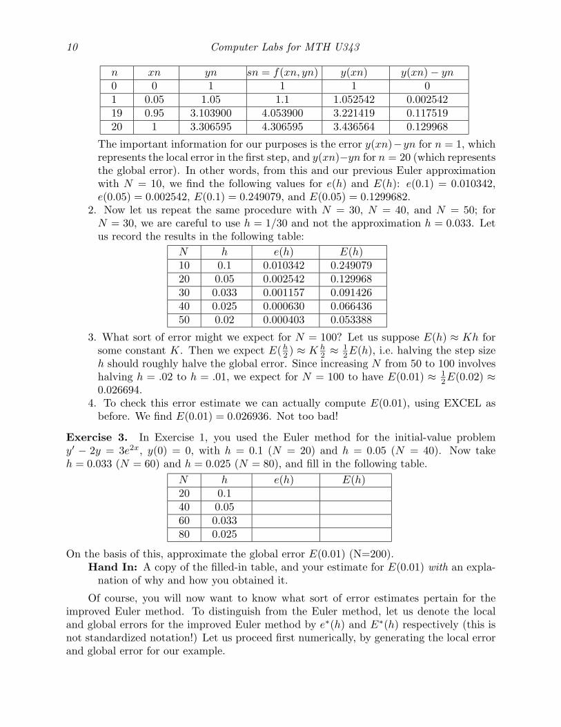
n xn yn sn = f(xn, yn) y(xn) y(xn) − yn0 0 1 1 1 01 0.05 1.05 1.1 1.052542 0.00254219 0.95 3.103900 4.053900 3.221419 0.11751920 1 3.306595 4.306595 3.436564 0.129968

The important information for our purposes is the error y(xn)−yn for n = 1, whichrepresents the local error in the first step, and y(xn)−yn for n = 20 (which representsthe global error). In other words, from this and our previous Euler approximationwith N = 10, we find the following values for e(h) and E(h): e(0.1) = 0.010342,e(0.05) = 0.002542, E(0.1) = 0.249079, and E(0.05) = 0.1299682.

2. Now let us repeat the same procedure with N = 30, N = 40, and N = 50; forN = 30, we are careful to use h = 1/30 and not the approximation h = 0.033. Letus record the results in the following table:

N h e(h) E(h)10 0.1 0.010342 0.24907920 0.05 0.002542 0.12996830 0.033 0.001157 0.09142640 0.025 0.000630 0.06643650 0.02 0.000403 0.053388

3. What sort of error might we expect for N = 100? Let us suppose E(h) ≈ Kh forsome constant K. Then we expect E(h

2 ) ≈ K h2 ≈ 1

2E(h), i.e. halving the step sizeh should roughly halve the global error. Since increasing N from 50 to 100 involveshalving h = .02 to h = .01, we expect for N = 100 to have E(0.01) ≈ 1

2E(0.02) ≈0.026694.

4. To check this error estimate we can actually compute E(0.01), using EXCEL asbefore. We find E(0.01) = 0.026936. Not too bad!

Exercise 3. In Exercise 1, you used the Euler method for the initial-value problemy′ − 2y = 3e2x, y(0) = 0, with h = 0.1 (N = 20) and h = 0.05 (N = 40). Now takeh = 0.033 (N = 60) and h = 0.025 (N = 80), and fill in the following table.

N h e(h) E(h)20 0.140 0.0560 0.03380 0.025

On the basis of this, approximate the global error E(0.01) (N=200).Hand In: A copy of the filled-in table, and your estimate for E(0.01) with an expla-

nation of why and how you obtained it.

Of course, you will now want to know what sort of error estimates pertain for theimproved Euler method. To distinguish from the Euler method, let us denote the localand global errors for the improved Euler method by e∗(h) and E∗(h) respectively (this isnot standardized notation!) Let us proceed first numerically, by generating the local errorand global error for our example.


Example 1 (cont’d). Compare the local error and global error for various step sizes inthe improved Euler approximations of the solution of y′ = x+ y, y(0) = 1, taking N = 10,N = 20, N = 30, N = 40, and N = 50. Based on these, what errors would you expect forN = 100?

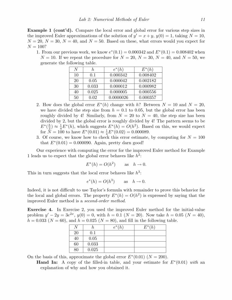
1. From our previous work, we know e∗(0.1) = 0.000342 and E∗(0.1) = 0.008402 whenN = 10. If we repeat the procedure for N = 20, N = 30, N = 40, and N = 50, wegenerate the following table.

N h e∗(h) E∗(h)10 0.1 0.000342 0.00840220 0.05 0.000042 0.00218230 0.033 0.000012 0.00098240 0.025 0.000005 0.00055650 0.02 0.0000026 0.000357

2. How does the global error E∗(h) change with h? Between N = 10 and N = 20,we have divided the step size from h = 0.1 to 0.05, but the global error has beenroughly divided by 4! Similarly, from N = 20 to N = 40, the step size has beendivided by 2, but the global error is roughly divided by 4! The pattern seems to beE∗(h

2 ) ≈ 14E

∗(h), which suggests E∗(h) = O(h2). Based on this, we would expectfor N = 100 to have E∗(0.01) ≈ 1

4E∗(0.02) = 0.000089.

3. Of course, we know how to check this error estimate, by computing for N = 100that E∗(0.01) = 0.000090. Again, pretty darn good!

Our experience with computing the error for the improved Euler method for Example1 leads us to expect that the global error behaves like h2:

E∗(h) = O(h2) as h → 0.

This in turn suggests that the local error behaves like h3:

e∗(h) = O(h3) as h → 0.

Indeed, it is not difficult to use Taylor’s formula with remainder to prove this behavior forthe local and global errors. The property E∗(h) = O(h2) is expressed by saying that theimproved Euler method is a second-order method.

Exercise 4. In Exercise 2, you used the improved Euler method for the initial-valueproblem y′ − 2y = 3e2x, y(0) = 0, with h = 0.1 (N = 20). Now take h = 0.05 (N = 40),h = 0.033 (N = 60), and h = 0.025 (N = 80), and fill in the following table.

N h e∗(h) E∗(h)20 0.140 0.0560 0.03380 0.025

On the basis of this, approximate the global error E∗(0.01) (N = 200).Hand In: A copy of the filled-in table, and your estimate for E∗(0.01) with an

explanation of why and how you obtained it.

Computer Lab 3: The Runge-Kutta Method

In Lab 2, we encountered Euler’s method and the improved Euler method as iterationschemes to approximate the solutions of first-order differential equations. However, thereis another iteration scheme which is far more accurate than either of these; in fact, theRunge-Kutta method is used to plot solution curves in the program Diffs used in Lab 1.Although the Runge-Kutta iteration scheme appears to be rather complicated, it is simplybased on Simpson’s Rule for numerical integration. Recall that if we approximate thegraph of u(x) on the interval [x0, x0 +h] by the parabola passing through the three valuesu(x0), u(x0 + h/2), u(x0 + h), then

(1)∫ x0+h

x0

u(x)dx ≈ h

6[u(x0) + 4u(x0 +

h

2) + u(x0 + h)].

I. THE RUNGE-KUTTA METHOD. Suppose we want to approximate the solutionof the initial-value problem

(2)

dy

dx= f(x, y)

y(x0) = y0.

Let us apply (1) to u(x) = y′(x) and x0 + h = x1:

(3)y(x1) − y(x0) =

∫ x1

x0

y′(x)dx

≈ h

6(y′(x0) + 2y′(x0 +

h

2) + 2y′(x0 +

h

2) + y′(x1))

where we have split up 4y′(x0 + h2 ) into two parts because we shall approximate them

differently. But equation (2) suggests that we take

(4) y1 = y0 +h

6(k1 + 2k2 + 2k3 + k4)

as an approximation for y(x1), where k1, k2, k3, k4 are approximations of the slope at theappropriate values of x. In fact, we shall take

(5)

k1 = f(x0, y0)

k2 = f(x0 +h

2, y0 +

h

2k1)

k3 = f(x0 +h

2, y0 +

h

2k2)

k4 = f(x1, y0 + hk3).

13


Notice that k1 = y′(x0), and k2 is the slope of y at the point produced by the Euler methodon [x0, x0 + h/2]; this much is similar to the improved Euler method. In fact, k3 is justthe slope of y at the point produced by the Euler method on [x0, x0 + h/2] with slopek2 instead of k1, and k4 is the slope of y at the point produced by the Euler method on[x0, x1] with slope k3.

The formulas (4) and (5) give us the value of y1, which we can then use to computey2, etc. However, the Runge-Kutta method is so good, we shall not need to take the valueh as small as we did for the Euler and improved Euler methods. This means that fewersteps need to be taken to get a good approximation of y(x).

Let us use the Runge-Kutta method on the same equation as we encountered in theExample of Lab 2:

Example 1. Use the Runge-Kutta method to approximate the solution of y′ = x + y,y(0) = 1 with step size h = 0.5 on the interval 0 ≤ x ≤ 1.

1. In your worksheet (in EXCEL or other spreadsheet program), create seven columnslabelled n, xn, yn, k1, k2, k3, and k4.

2. In the n column, enter 3 rows: 0 in cell A2, 1 in cell A3, and 2 in cell A4.3. In the xn column, enter 3 rows for the values x = 0, 0.5, and 1: 0 in cell B2,

“=B2+.5” and ENTER in cell B3, and Fill Down B3 into B4.4. In the yn column, enter 3 rows: 1 in cell C2 for the initial condition y0 = y(0) = 1,

”=C2+.5*(D2+2*E2+2*F2+G2)/6” and ENTER in cell C3 to implement equation(4), and then Fill Down C3 into C4.

5. To assign the values for k1, k2, k3, k4, first consider n = 0, and assign the values

k1 = x0 + y0 (in cell D2 type “=B2+C2” and ENTER),k2 = x0 + .25 + y0 + .25 · k1 (“=B2+.25+C2+.25*D2”),k3 = x0 + .25 + y0 + .25 · k2 (“=B2+.25+C2+.25*E2”),k4 = x1 + y0 + .5 · k3 (“=B3+C2+.5*F2”).

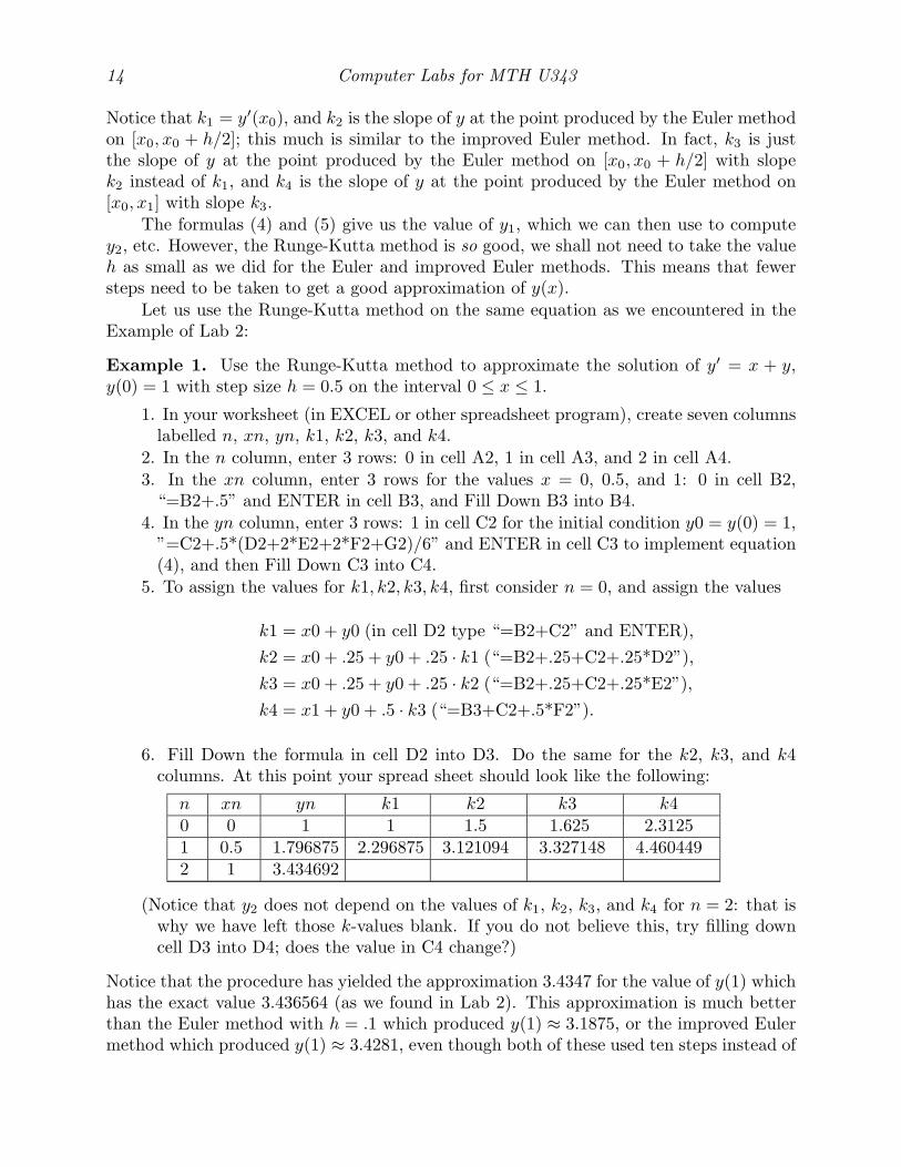
6. Fill Down the formula in cell D2 into D3. Do the same for the k2, k3, and k4columns. At this point your spread sheet should look like the following:

n xn yn k1 k2 k3 k40 0 1 1 1.5 1.625 2.31251 0.5 1.796875 2.296875 3.121094 3.327148 4.4604492 1 3.434692

(Notice that y2 does not depend on the values of k1, k2, k3, and k4 for n = 2: that iswhy we have left those k-values blank. If you do not believe this, try filling downcell D3 into D4; does the value in C4 change?)

Notice that the procedure has yielded the approximation 3.4347 for the value of y(1) whichhas the exact value 3.436564 (as we found in Lab 2). This approximation is much betterthan the Euler method with h = .1 which produced y(1) ≈ 3.1875, or the improved Eulermethod which produced y(1) ≈ 3.4281, even though both of these used ten steps instead of

Lab 3: The Runge-Kutta Method 15

the two steps employed by Runge-Kutta. Conclusion: Runge-Kutta is much more efficientthan the Euler methods.

Exercise 1. In Lab 2, we used the Euler and improved Euler methods to approximate y(2)for the solution of y′−2y = 3e2x with various values of h (h = 0.1, 0.05, 0.033 . . . , 0.025).Use the Runge-Kutta method with h = 0.1 to approximate y(2). How does this comparewith the Euler and Improved Euler methods?

Hand In: A printout of your worksheet for the Runge-Kutta method, and youranswer to the question.

Exercise 2. Consider the initial-value problem: y′ = (x+ y)/x, y(1) = 1.(a) Use the Runge-Kutta method with h = .5 to approximate the solution’s value atx = 2.

(b) Solve the equation by hand and compare the actual value y(2) to the approximationobtained in (a).

(Your approximation should be within .001 of the actual value; if not, you must havemade a mistake – find it!)

Hand In: A printout of your worksheet for the Runge-Kutta method in (a), anddetails of your solution by hand in (b).

Numerical methods can be misleading when singularities are involved: this is one goodreason for being able to solve equations by hand. The next exercise illustrates this fact.

Exercise 3. Consider the initial-value problem: y′ = y2, y(0) = 3/2.(a) Using the Runge-Kutta method with h = .5, what value do you get as an approx-

imation for the solution at x = 1? Are you suspicious that something is wrong?(b) Try using DIFFS to investigate the behavior of the solution. What do you suspect

is going on?(c) Find the actual solution by hand. Now can you explain what has happened?Hand In: A printout of your worksheet in (a), and an explanation (citing your

experiences in (b) and (c)) for what is going on.

II. EQUATIONS WHICH CANNOT BE SOLVED “BY HAND”. Up to thispoint, we have used numerical methods on equations that we can also solve by hand; thiswas done so that we could check the accuracy of the method. Of course, the whole reasonfor numerical methods is to be able to numerically approximate the solutions of equationswhich cannot be solved by hand. Let us consider an example.

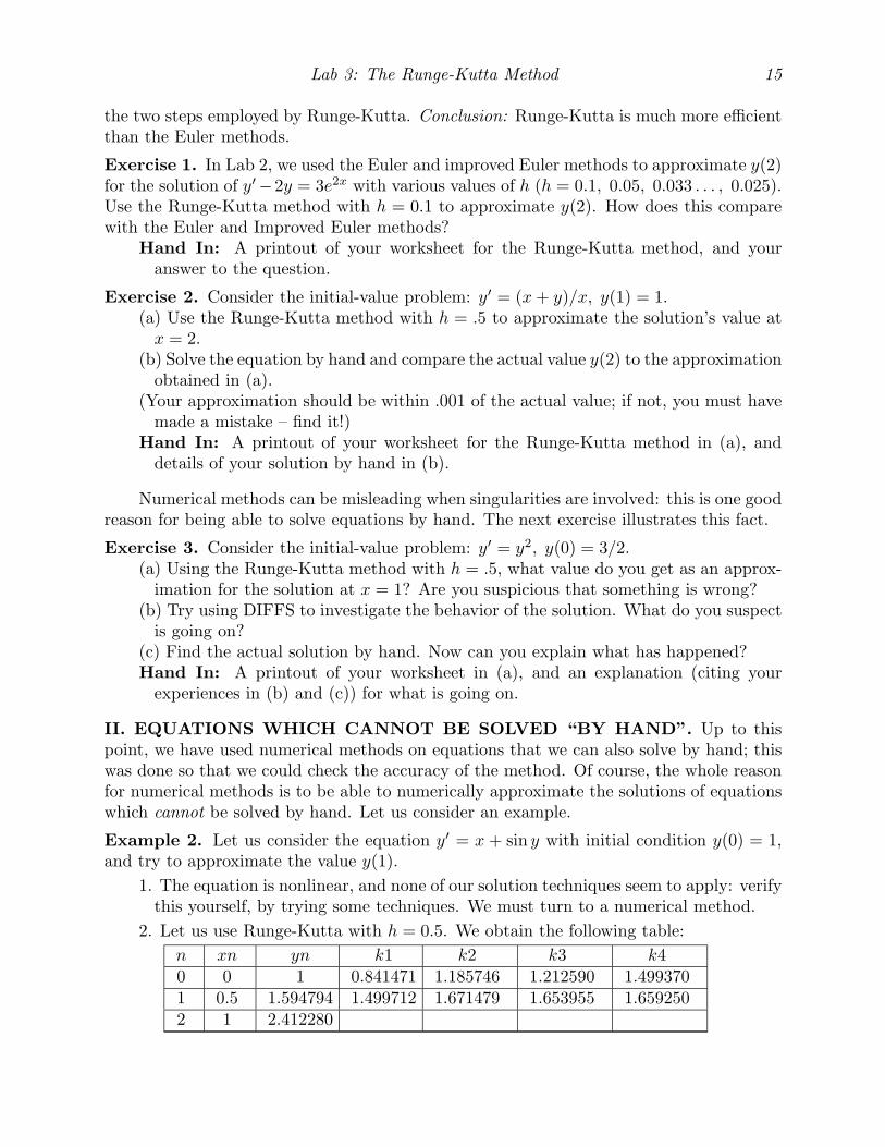
Example 2. Let us consider the equation y′ = x + sin y with initial condition y(0) = 1,and try to approximate the value y(1).

1. The equation is nonlinear, and none of our solution techniques seem to apply: verifythis yourself, by trying some techniques. We must turn to a numerical method.

2. Let us use Runge-Kutta with h = 0.5. We obtain the following table:n xn yn k1 k2 k3 k40 0 1 0.841471 1.185746 1.212590 1.4993701 0.5 1.594794 1.499712 1.671479 1.653955 1.6592502 1 2.412280


3. Naturally, we wonder how accurate is our answer y(1) ≈ y2 = 2.412280? We cannotsolve the equation by hand to check the accuracy, so what do we do? Let us tryRunge-Kutta with h = 0.25. We obtain the following table:

n xn yn k1 k2 k3 k40 0 1 0.841471 1.018547 1.028265 1.2011891 0.25 1.255678 1.200760 1.361415 1.364514 1.4996622 .5 1.595357 1.499698 1.602607 1.599819 1.6612383 .75 1.993931 1.661806 1.682520 1.680990 1.6649404 1 2.412838

Notice that y(1) ≈ y4 = 2.412838 agrees with the previous value 2.412280 to threedecimal places. We are fairly confident, therefore, that the approximation y(1) ≈2.412 is accurate to within ±0.001; suppose we want to do better.

4. Let us try Runge-Kutta with h = 0.1. Without displaying the table, the answer is2.41287465. This agrees with the previous value 2.412838 to four decimal places.

Exercise 4. Consider the initial-value problem y′ = x2 + cos y, y(0) = 0.(a) Use Runge-Kutta with h = 0.5 and h = 0.25 to approximate the value y(1). Givey(1) to as many decimal places as you feel is accurate.

(b) Use Runge-Kutta with h = 0.1 to approximate the value y(1), and give the valueto as many decimal places as you feel is accurate.

Hand In: A printout of your worksheet for the Runge-Kutta method with h =0.5, 0.25, 0.1, and the values of y(1) requested in (a) and (b).

III. ERROR ESTIMATES. Using Taylor series, it can be shown that the value y1,which is produced by the Runge-Kutta prescription (4)-(5), agrees with the the value atx1 of the fourth-order Taylor polynomial of y computed at a = x0. By Taylor’s formulawith remainder, this means that

(6) y1 − y(x1) = y(5)(c)h5

5!,

for some x0 < c < x1 = x0 + h. Applying the same reasoning as for the Euler method, weconclude that the local error for Runge-Kutta satisfies

(7) e(h) = O(h5) as h → 0,

and therefore the global error satisfies

(8) E(h) = O(h4) as h → 0.

For this reason, the Runge-Kutta is sometimes called the fourth-order Runge-Kutta method.In fact, there are even higher-order methods, but we shall not discuss them.

Let us see how to use (8) in Example 2 where we cannot solve the equation by hand.

Example 2 (cont’d). Use (8) to estimate the global errors in our Runge-Kutta approx-imations for the solutions of y′ = x+ sin y, y(0) = 1.

Lab 3: The Runge-Kutta Method 17

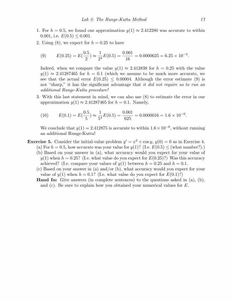
1. For h = 0.5, we found our approximation y(1) ≈ 2.412280 was accurate to within0.001, i.e. E(0.5) ≤ 0.001.

2. Using (8), we expect for h = 0.25 to have

(9) E(0.25) = E(0.52

) ≈ 124E(0.5) =

0.00116

= 0.0000625 = 6.25 × 10−5.

Indeed, when we compare the value y(1) ≈ 2.412838 for h = 0.25 with the valuey(1) ≈ 2.41287465 for h = 0.1 (which we assume to be much more accurate, wesee that the actual error E(0.25) ≤ 0.00004. Although the error estimate (9) isnot “sharp,” it has the significant advantage that it did not require us to run anadditional Runge-Kutta procedure!

3. With this last statement in mind, we can also use (8) to estimate the error in ourapproximation y(1) ≈ 2.41287465 for h = 0.1. Namely,

(10) E(0.1) = E(0.55

) ≈ 154E(0.5) =

0.001625

= 0.0000016 = 1.6 × 10−6.

We conclude that y(1) = 2.412875 is accurate to within 1.6×10−6, without runningan additional Runge-Kutta!

Exercise 5. Consider the initial-value problem y′ = x2 + cos y, y(0) = 0 as in Exercise 4.(a) For h = 0.5, how accurate was your value for y(1)? (I.e. E(0.5) ≤ (what number?).)(b) Based on your answer in (a), what accuracy would you expect for your value ofy(1) when h = 0.25? (I.e. what value do you expect for E(0.25)?) Was this accuracyachieved? (I.e. compare your values of y(1) between h = 0.25 and h = 0.1.

(c) Based on your answer in (a) and/or (b), what accuracy would you expect for yourvalue of y(1) when h = 0.1? (I.e. what value do you expect for E(0.1)?)

Hand In: Give answers (in complete sentences) to the questions asked in (a), (b),and (c). Be sure to explain how you obtained your numerical values for E.

Computer Lab 4: Numerical Methods for Systems

The numerical methods, which we have used to obtain numerical values for solutions ofa first-order equation, work equally well for a system of first-order equations. For example,consider functions x(t) and y(t) of the variable t, which are desired to satisfy the twofirst-order equations

(1)

dx

dt= f(t, x, y)

dy

dt= g(t, x, y).

We can change notation by letting x1 = x, x2 = y, f1 = f and f2 = g:

(2)

dx1

dt= f1(t, x1, x2)

dx2

dt= f2(t, x1, x2).

The equation (2) may also be written in vector notation as

(3)d#x

dt= #f(t, #x)

where

#x =(x1

x2

)and #f =

(f1

f2

).

In the formulation (3), it is clear that we could just as easily consider any number m ofequations in the same number of variables: use #x = (x1, . . . , xm) and #f = (f1, . . . , fm);but for the purposes of this lab we shall always take m = 2, and generally prefer (1) over(2) or (3) to avoid using subscripts which may be confused with the iteration steps. Ofcourse, we generally want to solve a first-order system given an initial condition at t = 0:#x(0) = #x0 for (3), or x(0) = x0 and y(0) = y0 for (1).

As we did for first-order equations, we shall call a system autonomous when theindependent variable t does not occur explicitly. Thus (3) is autonomous when it is ofthe form d#x/dt = #f(#x); moreover, a critical point #x0 which satisfies #f(#x0) = 0 yields anequilibrium solution of the form #x(t) ≡ #x0. Similarly, (1) is autonomous when it is of theform

(4)

dx

dt= f(x, y)

dy

dt= g(x, y),

and an equilibrium solution is of the form (x(t), y(t)) ≡ (x0, y0) where (x0, y0) is a crit-ical point: f(x0, y0) = 0 and g(x0, y0) = 0. Autonomous systems occur frequently in

19


applications, and equilibrium solutions generally play a significant role in the applica-tion, especially when they are stable (recall this means that solutions that begin near theequilibrium remain near it as t → ∞).

Now suppose we want to find x(t) and y(t) satisfying (1) and the initial conditionsx(0) = x0 and y(0) = y0. Given a step size h, the iteration scheme will show how to usex0 and y0 to obtain x1 and y1 which should be approximations for the exact values x(h)and y(h). Then x1 and y1 can be used to find x2 and y2 as approximations for x(2h) andy(2h), etc.

I. EULER’S METHOD. For a step size h, Euler’s method for (3) may be expressed by#xn+1 = #xn + h#f(t, #x). For (1) we obtain:

(5)xn+1 = xn + hf(tn, xn, yn)yn+1 = yn + hg(tn, yn, yn).

Example 1. Let us consider

(6)

dx

dt= x− 3y x(0) = 2

dy

dt= 2x− 4y y(0) = 1.

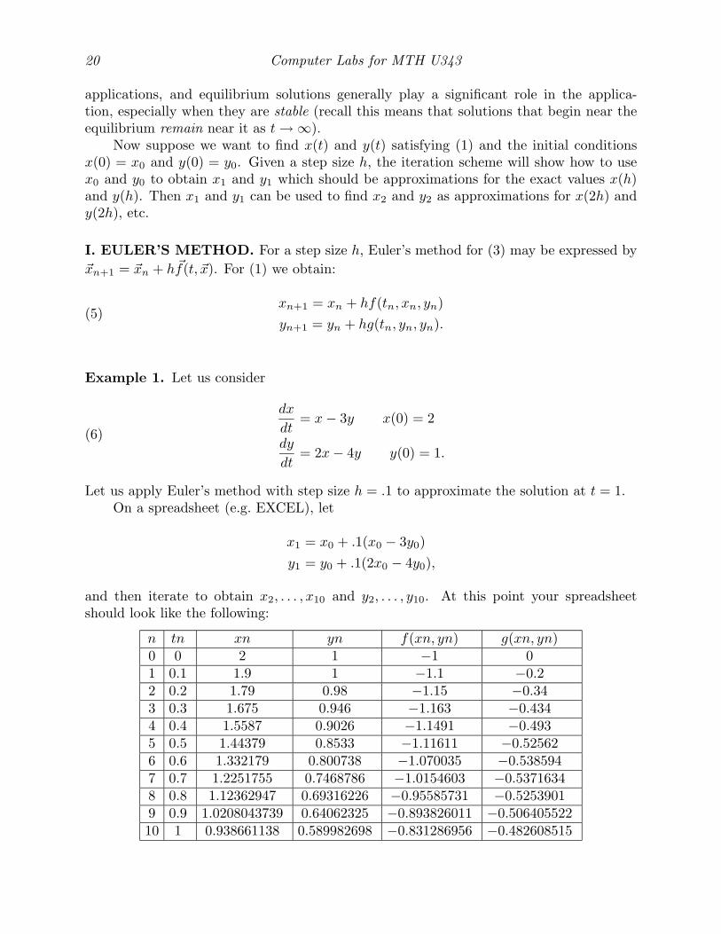
Let us apply Euler’s method with step size h = .1 to approximate the solution at t = 1.On a spreadsheet (e.g. EXCEL), let

x1 = x0 + .1(x0 − 3y0)y1 = y0 + .1(2x0 − 4y0),

and then iterate to obtain x2, . . . , x10 and y2, . . . , y10. At this point your spreadsheetshould look like the following:

n tn xn yn f(xn, yn) g(xn, yn)0 0 2 1 −1 01 0.1 1.9 1 −1.1 −0.22 0.2 1.79 0.98 −1.15 −0.343 0.3 1.675 0.946 −1.163 −0.4344 0.4 1.5587 0.9026 −1.1491 −0.4935 0.5 1.44379 0.8533 −1.11611 −0.525626 0.6 1.332179 0.800738 −1.070035 −0.5385947 0.7 1.2251755 0.7468786 −1.0154603 −0.53716348 0.8 1.12362947 0.69316226 −0.95585731 −0.52539019 0.9 1.0208043739 0.64062325 −0.893826011 −0.50640552210 1 0.938661138 0.589982698 −0.831286956 −0.482608515

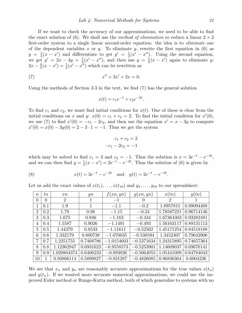
Lab 4: Numerical Methods for Systems 21

If we want to check the accuracy of our approximations, we need to be able to findthe exact solution of (6). We shall use the method of elimination to reduce a linear 2 × 2first-order system to a single linear second-order equation: the idea is to eliminate oneof the dependent variables x or y. To eliminate y, rewrite the first equation in (6) asy = 1

3 (x − x′) and differentiate to get y′ = 13 (x′ − x′′). Using the second equation,

we get y′ = 2x − 4y = 13 (x′ − x′′), and then use y = 1

3 (x − x′) again to eliminate y:2x− 4

3 (x− x′) = 13 (x′ − x′′) which can be rewritten as

(7) x′′ + 3x′ + 2x = 0.

Using the methods of Section 3.3 in the text, we find (7) has the general solution

x(t) = c1e−t + c2e

−2t.

To find c1 and c2, we must find initial conditions for x(t). One of these is clear from theinitial conditions on x and y: x(0) = c1 + c2 = 2. To find the initial condition for x′(0),we use (7) to find x′(0) = −c1 − 2c2, and then use the equation x′ = x − 3y to computex′(0) = x(0) − 3y(0) = 2 − 3 · 1 = −1. Thus we get the system

c1 + c2 = 2−c1 − 2c2 = −1

which may be solved to find c1 = 3 and c2 = −1. Thus the solution is x = 3e−t − e−2t,and we can then find y = 1

3 (x− x′) = 2e−t − e−2t. Thus the solution of (6) is given by

(8) x(t) = 3e−t − e−2t and y(t) = 2e−t − e−2t.

Let us add the exact values of x(t1), . . . , x(t10) and y1, . . . , y10 to our spreadsheet:

n tn xn yn f(xn, yn) g(xn, yn) x(tn) y(tn)0 0 2 1 −1 0 2 11 0.1 1.9 1 −1.1 −0.2 1.8957815 0.990944082 0.2 1.79 0.98 −1.15 −0.34 1.78587221 0.967141463 0.3 1.675 0.946 −1.163 −0.434 1.67364303 0.932824814 0.4 1.5587 0.9026 −1.1491 −0.493 1.56163117 0.891311135 0.5 1.44379 0.8533 −1.11611 −0.52562 1.45171254 0.845181886 0.6 1.332179 0.800738 −1.070035 −0.538594 1.3452407 0.796429067 0.7 1.2251755 0.7468786 −1.0154603 −0.5371634 1.24315895 0.746573648 0.8 1.12362947 0.6931623 −0.9558573 −0.5253901 1.14609037 0.696761419 0.9 1.020804374 0.6406233 −0.893826 −0.5064055 1.05441009 0.6478404310 1 0.93866114 0.5899827 −0.831287 −0.4826085 0.96830304 0.6004236

We see that xn and yn are reasonably accurate approximations for the true values x(tn)and y(tn). If we wanted more accurate numerical approximations, we could use the im-proved Euler method or Runge-Kutta method, both of which generalize to systems with no


additional effort. However, the spreadsheet becomes more complicated, so we shall confineour study of numerical methods for systems to Euler’s method.

Notice that x(tn), y(tn), xn, and yn all are decreasing in tn. What happens as t → ∞?Let us expand our spreadsheet (simply by filling down):

n tn xn yn f(xn, yn) g(xn, yn) x(tn) y(tn)0 0 2 1 −1 0 2 11 0.1 1.9 1 −1.1 −0.2 1.8957815 0.990944082 0.2 1.79 0.98 −1.15 −0.34 1.78587221 0.967141463 0.3 1.675 0.946 −1.163 −0.434 1.67364303 0.932824814 0.4 1.5587 0.9026 −1.1491 −0.493 1.56163117 0.891311135 0.5 1.44379 0.8533 −1.11611 −0.52562 1.45171254 0.845181886 0.6 1.332179 0.800738 −1.070035 −0.538594 1.3452407 0.796429067 0.7 1.2251755 0.7468786 −1.0154603 −0.5371634 1.24315895 0.746573648 0.8 1.12362947 0.6931623 −0.9558573 −0.5253901 1.14609037 0.696761419 0.9 1.020804374 0.6406233 −0.893826 −0.5064055 1.05441009 0.6478404310 1 0.93866114 0.5899827 −0.831287 −0.4826085 0.96830304 0.600423611 1.1 0.85553244 0.5417218 −0.7696331 −0.4558225 0.88781009 0.5549390112 1.2 0.77856913 0.4961396 −0.7098497 −0.4274201 0.81286468 0.5116704713 1.3 0.70758417 0.4533976 −0.6526086 −0.398422 0.7433218 0.4707900114 1.4 0.64232331 0.4135554 −0.5983428 −0.3695749 0.67898083 0.4323838715 1.5 0.58248902 0.3765979 −0.5473047 −0.3414135 0.61960341 0.3964732516 1.6 0.52775856 0.3424565 −0.4996111 −0.314309 0.56492735 0.3630308317 1.7 0.47779745 0.3110256 −0.4552795 −0.2885076 0.5146773 0.3319937818 1.8 0.43226951 0.2821749 −0.4142551 −0.2641605 0.46857294 0.3032740519 1.9 0.390844 0.2557588 −0.3764325 −0.2413473 0.42633509 0.2767664720 2.0 0.35320075 0.2316241 −0.3416715 −0.2200949 0.38769021 0.25235493

It looks like x and y are tending to zero as t → ∞. This seems particularly likely if we noticethat (0, 0) is an equilibrium solution for the system. In fact, solving f(x, y) = x− 3y = 0and g(x, y) = 2x − 4y = 0 shows that x = 0 = y is the only equilibrium solution. Is theequilibrium asymptotically stable, i.e. does every solution which begins near (0, 0) tend to(0, 0) as t → ∞? We cannot answer this question by looking at our spreadsheet, nor evenby changing the initial conditions x(0) = 2 and y(0) = 1 to other values and creating manysuch spreadsheets. The only way to tell that all solutions tend to (0, 0) is to look at thegeneral solution x(t) = c1e

−t + c2e−2t and y(t) = 1

3 (x(t) − x′(t)) = 23c1e

−t + c2e−2t: for

all values of the constants c1 and c2, we have x(t), y(t) → 0 as t → ∞, so the equilibriumis stable.

Exercise 1. Consider the system

dx

dt= x+ 2y

dy

dt= 2x+ y + 3


with the initial conditions

x(0) = 1 and y(0) = 0.

(a) Use h = 0.01 to approximate the values of x(0.5) and y(0.5).(b) Use Fill Down in your spreadsheet to find approximations for x(1.0) and y(1.0).(c) Can you guess what happens to x(t) and y(t) as t → ∞?(d) Use the method of elimination to find the actual solution of this problem; you

will need to use Section 3.5 in the text. What are the actual values x(0.5), y(0.5),x(1.0), and y(1.0)?

(e) Find the critical point of the system. Determine if the equilibrium solution isasymptotically stable or unstable.

(f) Can you find new initial conditions (other than the equilibrium) for the system forwhich the solution (x(t), y(t)) approaches the critical point in the limit as t → ∞?

Hand In: A printout of your spreadsheet from (b), your answer to (c), your hand-written solution and the requested values for (d), and your answers to (e) and (f).

II. APPLICATION TO A PREDATOR-PREY MODEL. Systems of two first-order equations of the form

(9)

dx

dt= ax− bxy

dy

dt= −cy + dxy,

where a, b, c, and d are all positive constants, arise in many physical sciences. One instanceoccurs in biology and sociology in which two populations of animals interact as predatorsand prey. An example might be foxes and rabbits.

To understand the model (9), suppose that the x-population (the “prey”) grows ac-cording to dx/dt = ax when no predators are present (y = 0); rabbits, for example, arecertainly known for their ability to reproduce! Suppose, also, that the y-population (the“predators”) will die out according to dy/dt = −cy when no prey exist (x = 0); we mustimagine that the foxes only feed on rabbits. However, when both predators and prey ex-ist (x, y �= 0), then the number of encounters between the species is proportional to theproduct xy, and these encounters inhibit the growth of x (whence the term −bxy), butenhance the growth of y (whence the term +dxy).

Now let us take some specific values for a, b, c, and d. For example, when x and y aremeasured in “thousands” (i.e. x = 1 means “one thousand rabbits”), suppose a, b, c, andd all have the value 1. Then (9) becomes

(10)

dx

dt= x− xy

dy

dt= −y + xy.

To find critical points, we set f(x, y) = x − xy = x(1 − y) = 0 to obtain x = 0 or y = 1;similarly, g(x, y) = −y + xy = y(−1 + x) = 0 requires y = 0 or x = 1. We have two

Predator-Prey Example (h=0.2)

00.20 .40 .60 .8

11 .21 .4

0

0.8

1.6

2.4

3.2 4

4.8

5.6

6.4

7.2 8

xn

yn


possibilities for critical points: (x, y) = (0, 0) or (x, y) = (1, 1). When (x, y) = (0, 0),both populations are zero, and of course remain zero. The value (x, y) = (1, 1) is moreinteresting, because it indicates that if initially there are exactly 1, 000 rabbits and 1, 000foxes, then the populations remain constant. Is this a stable equilibrium solution? Let usfind out.

Let us take initial conditions close to the critical point (1, 1), for example

(11) x(0) = 0.9 y(0) = 1.1,

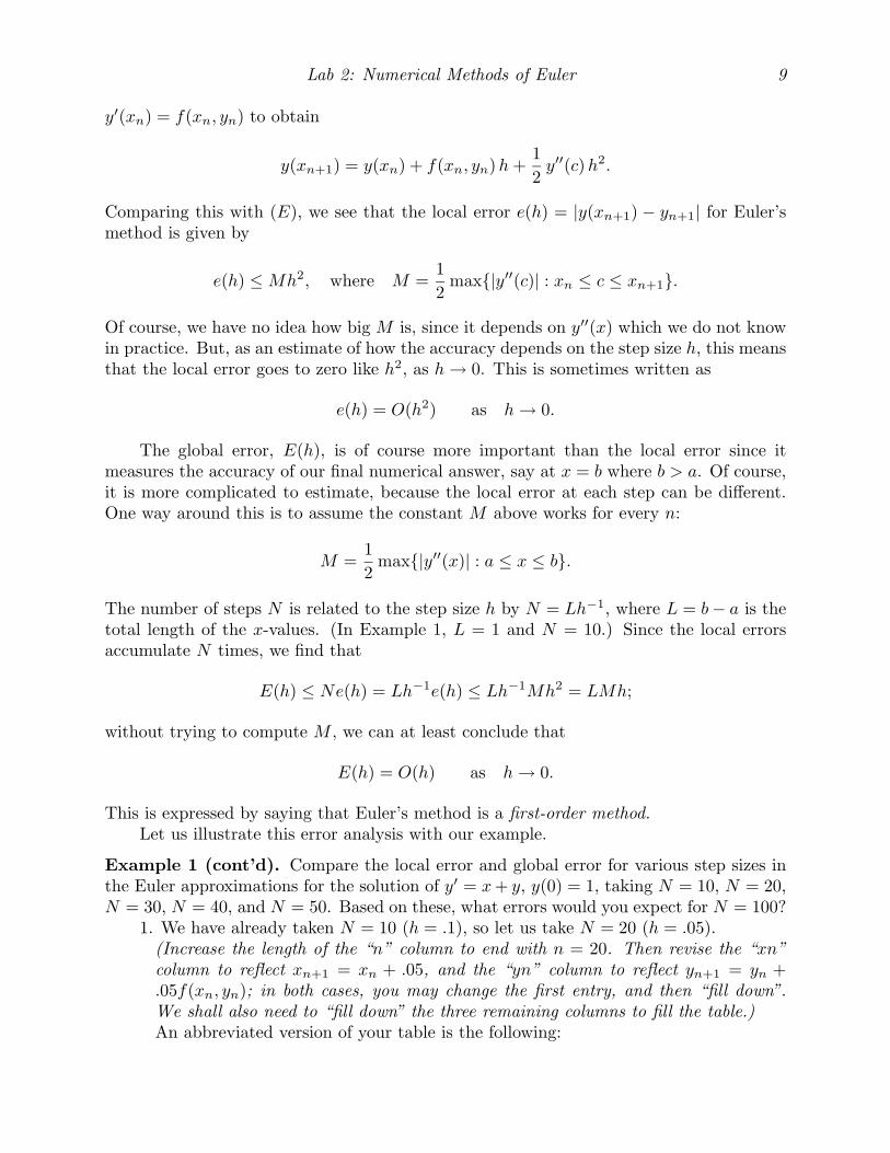
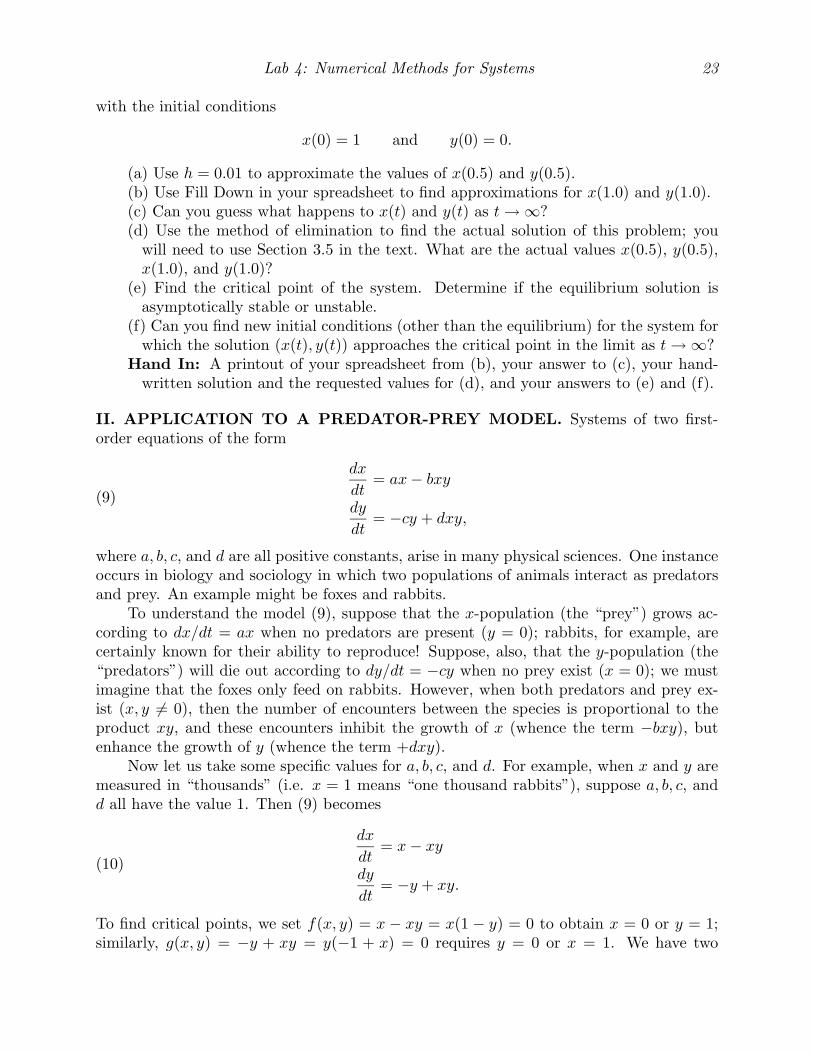
and use Euler’s method to study the solution. Let us take step size h = 0.2. The followingis an abbreviated version of the results:

n tn xn yn f(xn, yn) g(xn, yn)0 0 0.9 1.1 −0.09 −0.111 0.2 0.882 1.078 −0.068796 −0.1272042 0.4 0.8682408 1.0525592 −0.04563404 −0.138684363 0.6 0.85911399 1.02482233 −0.02132521 −0.14438313

9 1.8 0.90641996 0.86945483 0.11832874 −0.0813636210 2.0 0.9300857 0.85318211 0.13655322 −0.05964963

14 2.8 1.05485282 0.83547109 0.17355379 0.0458279515 3.0 1.08956358 0.84463668 0.16927822 0.07564869

19 3.8 1.20410601 0.94142407 0.07053164 0.1921503120 4.0 1.21821234 0.97985413 0.02454195 0.21381626

Then let us use ChartWizard to graph the solutions through n = 40 (t = 8):


Now this is rather interesting. Notice that the populations both seem to oscillateabout the equlibrium solution, with the predator population y lagging behind the preypopulation x: once the prey population starts to increase, it takes a while for the predatorpopulation to begin increasing; but then it catches up with the prey population, whichhas begun to decrease. All this is quite reasonable for the behavior of populations ofspecies, and leads us to define the values x = 1 and y = 1 (from the equilibrium solution(x, y) = (1, 1)) as the average population values.

Exercise 2. Trying to control the rabbit population.(a) What do you think the effect would be of introducing a large number of foxes to try

to control the rabbit population? Introduce an additional 1, 000 foxes at t = 0 bychanging y(0) = 1.1 to y(0) = 2.1, and use EXCEL to numerically approximate thesolution with h = 0.2. Use Chart Wizard to plot the result. Did the introductionof additional foxes keep down the rabbit population?

(b) What do you think the effect would be of a one-time killing spree to control therabbit population? Reset y(0) = 1.1, but kill off half the rabbits at t = 0 by changingx(0) = .9 to x = .45, and use EXCEL to numerically approximate the solution withh = 0.2. Use Chart Wizard to plot the result. Did the one-time killing spree keepdown the rabbit population? What effect did it have on the fox population?

(c) Have the strategies in (a) or (b) changed the average population values of rabbitsand foxes?

Hand In: A printout of your spreadsheet and chart, along with your answer to thequestion in (a). Similarly, a printout of spreadsheet, chart, and answers to the twoquestions in (b). Finally, a short answer to the question in (c).

III. EFFECT OF TRAPPING. We conclude from Part II that changing the initialconditions by introducing more foxes or conducting a one-time killing spree is not an effec-tive means of controlling the rabbit population: the average value of the rabbit populationhas not been changed. How about setting traps for the rabbits? Suppose we can find abait for the trap which appeals to rabbits and not to foxes (carrots?). This may lead tothe modification of (9) as follows:

(12)

dx

dt= ax− bxy − ex

dy

dt= −cy + dxy.

Exercise 3. Still trying to control the rabbit population.(a) Explain in words why the term −ex in (12) might represent trapping better than

a term like −e.(b) Take a = b = c = d = 1 and e = .5 in (12), i.e. introduce trapping to the example

(10), and use the initial values (11). Use EXCEL to numerically approximate thesolution with h = 0.2, and Chart Wizard to plot the results.

(c) What effect has the setting of traps had on the average population values?Hand In: Your answer to (a) in complete sentences. A printout of spreadsheet and

chart in (b). Also, a short answer to the question in (c).

Lab 5: MATLAB and 2nd-order Differential Equations

We are now familiar with using a spreadsheet to set up numerical methods for ap-proximating solutions of a single differential equation and systems of differential equa-tions. However, there are several software packages which have these numerical algorithmsalready installed and ready to use. Such software packages are generally called “ODESolvers”. One such program is DIFFS, which we used in Lab 1; it is very easy to use, butit does not solve systems of equations. More powerful solvers, which do handle systems,are incorporated in computational software such as MATLAB.

In this computer lab, we shall not only learn how to use an ODE solver in MATLAB,but we shall apply it to compute and study the solutions of 2nd-order equations x′′ = f(t, x)or x′′ = f(t, x, x′).

I. APPLYING MATLAB TO 1st-ORDER EQUATIONS & SYSTEMS.MATLAB has several numerical procedures for computing the solutions of first-order

equations and systems of the form y′ = f(t, y); we shall concentrate on “ode45”, whichis a suped-up Runge-Kutta method. The first step is to enter the equation or system bycreating an “M-file” which contains the definition of your equation, and is given a namefor reference, such as “diffeqn” (the suffix “.m” will be added to identify it as an M-file.).The second step is to apply ode45 by using the syntax:

(1) [t, y] = ode45(′diffeqn′, [t0, tf ], y0);

where t0 is the initial time, tf is the final time, and y0 is the initial condition, y(t0) = y0.The same syntax (1) works for equations and systems alike.

Example 1. y′ = y2 − t, y(0) = 0, for 0 ≤ t ≤ 4.

1. Creating the M-file. Start up MATLAB; the Command Window appears with theprompt >> awaiting instructions. Choose New from the File menu, and select M-file.You are now in a text editor where you create MATLAB files. Enter the following text:

function ypr=example1(t,y)

ypr=y^2-t;

Name this M-file “example1.m” by selecting Save As from the File menu.

2. Running ode45. Return to the Command Window, and enter the following:

>> [t, y] = ode45(′example1′, [0, 4], 0);

MATLAB will do its computing, then give you another prompt.

3. Plotting the Solution. You can plot the solution y(t) by typing

>> plot(t, y)

27

0 1 2 3 4-2

-1.5

-1

-0.5

0

t

y

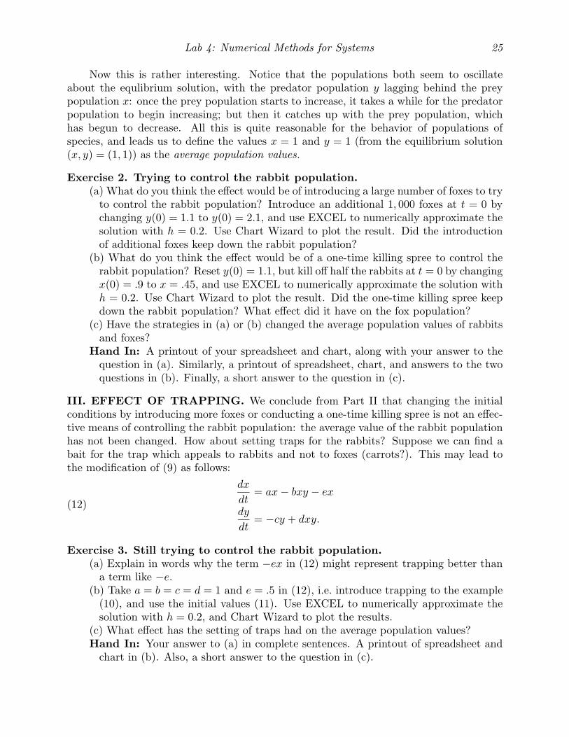
The solution to y'=y^2-t with y(0)=0.


and hitting the enter key. The following plot should appear on your screen:

To give your plot the title and axes labels in the picture above, type

>>title(′The solution to y′′ = y^2− t with y(0) = 0.′)>>xlabel(′t′)>>ylabel(′y′)

and hit the enter key after each line. Notice that each title/label is identified by singlequotation marks, e.g. ′The solution...′. Note: You might expect that the title line shouldread y′ = yˆ2− t instead of y′′ = yˆ2− t, but the former would indicate to MATLAB thatthe title ends with y′, so we must put in the extra single quote (i.e. two single quotes, notone double quote).

You can also have MATLAB tabulate the t-values it has selected and the y-values ithas computed by entering

>> [t, y]

in the Command Window. This should produce a vertical column of numbers, the last ofwhich is t = 4.0000 and y = −1.9311, i.e. y(4) = −1.9311 as appears in the plot.

Exercise 1. Consider the initial value problem y′ = t2 + cos y, y(0) = 0 which wasencountered in Exercise 4 of Lab 3. Use MATLAB to plot the solution for 0 ≤ t ≤ 1, andfind the approximate value of y(1).Hand In: A printout of your plot and the value of y(1).

Lab 5: MATLAB and 2nd-order Differential Equations 29

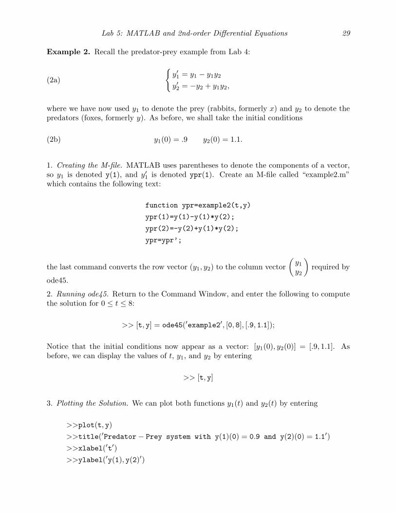
Example 2. Recall the predator-prey example from Lab 4:

(2a)

{y′1 = y1 − y1y2

y′2 = −y2 + y1y2,

where we have now used y1 to denote the prey (rabbits, formerly x) and y2 to denote thepredators (foxes, formerly y). As before, we shall take the initial conditions

(2b) y1(0) = .9 y2(0) = 1.1.

1. Creating the M-file. MATLAB uses parentheses to denote the components of a vector,so y1 is denoted y(1), and y′1 is denoted ypr(1). Create an M-file called “example2.m”which contains the following text:


ypr(1)=y(1)-y(1)*y(2);

ypr(2)=-y(2)+y(1)*y(2);

ypr=ypr’;

the last command converts the row vector (y1, y2) to the column vector(y1

y2

)required by

ode45.

2. Running ode45. Return to the Command Window, and enter the following to computethe solution for 0 ≤ t ≤ 8:

>> [t, y] = ode45(′example2′, [0, 8], [.9, 1.1]);

Notice that the initial conditions now appear as a vector: [y1(0), y2(0)] = [.9, 1.1]. Asbefore, we can display the values of t, y1, and y2 by entering

>> [t, y]

3. Plotting the Solution. We can plot both functions y1(t) and y2(t) by entering

>>plot(t, y)>>title(′Predator− Prey system with y(1)(0) = 0.9 and y(2)(0) = 1.1′)>>xlabel(′t′)>>ylabel(′y(1), y(2)′)

0 2 4 6 80.85

0.9

0.95

1

1.05

1.1

1.15

t

y

Predator-prey system with y(1)(0)=0.9 and y(2)(0)=1.1.


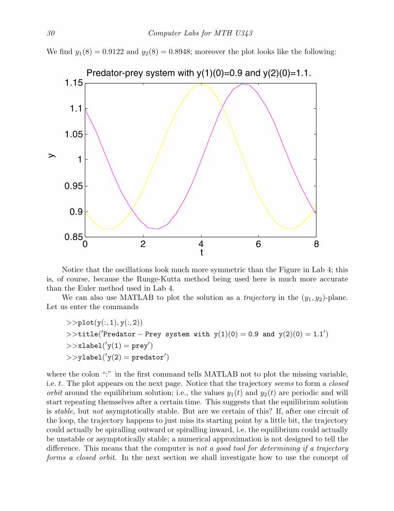
We find y1(8) = 0.9122 and y2(8) = 0.8948; moreover the plot looks like the following:

Notice that the oscillations look much more symmetric than the Figure in Lab 4; thisis, of course, because the Runge-Kutta method being used here is much more accuratethan the Euler method used in Lab 4.

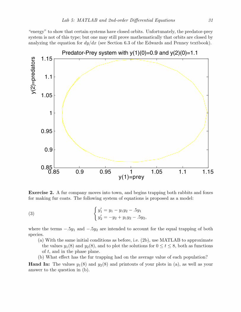
We can also use MATLAB to plot the solution as a trajectory in the (y1, y2)-plane.Let us enter the commands

>>plot(y(:, 1), y(:, 2))>>title(′Predator− Prey system with y(1)(0) = 0.9 and y(2)(0) = 1.1′)>>xlabel(′y(1) = prey′)>>ylabel(′y(2) = predator′)

where the colon “:” in the first command tells MATLAB not to plot the missing variable,i.e. t. The plot appears on the next page. Notice that the trajectory seems to form a closedorbit around the equilibrium solution; i.e., the values y1(t) and y2(t) are periodic and willstart repeating themselves after a certain time. This suggests that the equilibrium solutionis stable, but not asymptotically stable. But are we certain of this? If, after one circuit ofthe loop, the trajectory happens to just miss its starting point by a little bit, the trajectorycould actually be spiralling outward or spiralling inward, i.e. the equilibrium could actuallybe unstable or asymptotically stable; a numerical approximation is not designed to tell thedifference. This means that the computer is not a good tool for determining if a trajectoryforms a closed orbit. In the next section we shall investigate how to use the concept of

0.85 0.9 0.95 1 1.05 1.1 1.150.85

0.9

0.95

1

1.05

1.1

1.15

y(1)=prey

y(2)

=pr

edat

ors

Predator-Prey system with y(1)(0)=0.9 and y(2)(0)=1.1


“energy” to show that certain systems have closed orbits. Unfortunately, the predator-preysystem is not of this type; but one may still prove mathematically that orbits are closed byanalyzing the equation for dy/dx (see Section 6.3 of the Edwards and Penney textbook).

Exercise 2. A fur company moves into town, and begins trapping both rabbits and foxesfor making fur coats. The following system of equations is proposed as a model:

(3)

{y′1 = y1 − y1y2 − .5y1

y′2 = −y2 + y1y2 − .5y2,

where the terms −.5y1 and −.5y2 are intended to account for the equal trapping of bothspecies.

(a) With the same initial conditions as before, i.e. (2b), use MATLAB to approximatethe values y1(8) and y2(8), and to plot the solutions for 0 ≤ t ≤ 8, both as functionsof t, and in the phase plane.

(b) What effect has the fur trapping had on the average value of each population?Hand In: The values y1(8) and y2(8) and printouts of your plots in (a), as well as youranswer to the question in (b).


II. 2nd-ORDER EQUATIONS AND MECHANICAL VIBRATIONS.A second-order differential equation of the form

(4) x′′ = f(t, x, x′)

can be reduced to a system of first-order equations by the introduction of an additionaldependent variable. Using our vector notation, let

(5) y1 = x and y2 = y′1 = x′.

We can then write

(6)

{y′1 = y2

y′2 = f(t, y1, y2),

where the first equation explains the relationship between y1 and y2, and the secondequation is just (4). In this section we shall consider various special cases of (4) thatcorrespond to forced linear vibrations, damped and undamped, as well as free vibrationsthat may be nonlinear.

Linear VibrationsLinear vibrations may be represented by a spring-mass system

(7) mx′′ + cx′ + kx = F (t),

where m is mass, c is the damping constant, k is the spring constant, and F (t) is theforcing term. The equation (7) may be solved analytically using undetermined coefficientsas in Section 3.5 of the Edwards & Penney textbook, but we shall here use MATLAB tocompute and plot the solutions.

Example 3. Consider a forced, undamped vibration of the form (7) with m = 1 slug,c = 0, k = 4 lbs./ft, and F (t) = cosωt, where we shall specify the frequency ω below. Weshall also take zero initial conditions: x(0) = 0 = x′(0).

We convert this to a first-order system by taking y1 = x and y2 = x′:

(8)

{y′1 = y2

y′2 = cosωt− 4y1,

1. Creating the M-file. Create an M-file called “example3.m” containing the following text:


global w

ypr(1)=y(2);

ypr(2)=cos(w*t)-4*y(1);

ypr=ypr’

0 5 10 15 20-0.8

-0.6

-0.4

-0.2

0

0.2

0.4

0.6Forced, undamped vibration with w=1 on 0<t<20

t


The line “global w” means that we have defined ω or “w” to be a variable which we willspecify in the Command Window; this saves going back and changing the M-file everytimewe want to change the value of ω.2. Running ode45. Suppose we want to solve (8) with ω = 1 on the interval 0 ≤ t ≤ 20.Return to the Command Window, and enter the following:

>> global w

>> w = 1

>> [t, y] = ode45(′example3′, [0, 20], [0, 0]);

Notice that the first command calls up the global variable, and the second command assignsits value; the third command, of course, runs ode45.3. Plotting the Solution. If we enter the command plot(t,y), we will see both y1 and y2

plotted as functions of t. However, we are really only interested in x(t). For this reason,let us enter

>>x = y(:, 1);>>plot(t, x);>>title(′Forced, undamped vibration with w = 1 on 0 < t < 20′)>>xlabel(′t′)>>ylabel(′x′)

The resulting plot appears below:


Notice that resonance does not occur, nor do we see the “beats” that occur near resonance;this is because ω = 1 is not even close to the resonance frequency.

Exercise 3. Resonance and Beats.(a) Determine the value of ω that will produce resonance in (8).(b) With the resonance value of ω determined in part (a), use MATLAB to plot the

solution for 0 ≤ t ≤ 20. Do you see resonance?(c) Take ω close to the resonance value, differing say by 0.1, and use MATLAB to

plot the solution for 0 ≤ t ≤ 20. Describe what you see. Try increasing the timeinterval to 0 ≤ t ≤ 60 for both plots (i.e. the resonant and near-resonant values ofω). Now describe what you see.

Hand In: The value of the resonance frequency in part (a), and printouts of your all plotsfrom (b) and (c) with the answers to the questions asked.

Exercise 4. Damping & Practical Resonance. Consider a forced, damped vibrationof the form (7), where 0 < c2 < 4mk, so (7) is “underdamped”. The damping preventspure resonance, but if c is very small, we might expect practical resonance, i.e. oscillationsgrow in amplitude larger than the driving force (but do not become infinitely large).

(a) Let m = 1, k = 4, ω = 2, and c = .5. (Hint: Introduce a “global c” line in yourM-file; this will make (b) easier.) Compute and plot the solution for 0 ≤ t ≤ 30.After a time, all that remains should be a steady, periodic solution.

(b) Try changing c to the values .1 and .05. (You may also want to increase yourtime interval.) What do you observe about the amplitudes of the resulting steady,periodic solutions?

(c) Now fix c at the value .05, and vary ω through the values 1.9, 2.0, and 2.1. Whatdo you observe about the amplitudes of the resulting vibrations?

Hand In: Printouts of the plots for the various values of c and ω, and the answers to thequestions asked.

Nonlinear VibrationsMATLAB is particularly useful for solving (4) when F is nonlinear in x and/or x′,

since analytic methods may not be available. We shall concentrate on the relatively simpleequations of the form

(9) x′′ = f(x),

which is free (no forcing term) and conservative (no damping). For such equations, theconcept of energy is useful in showing that trajectories indeed form closed orbits. Supposethat F (x) is an antiderivative for f(x), i.e. F ′(x) = f(x), and consider the expression

(10) E(t) =12x′(t)2 − F (x(t)),

for a given solution x(t) of (9). If we differentiate (10) with respect to t, the chain rulegives us

dE

dt= x′x′′ − f(x)x′ = x′(x′′ − f(x)) = 0;


in other words, the quantity E is constant. E is usually called the “energy” of the solutionand so “conservation of energy” applies to (9). Of course, the value of E depends on theparticular solution x(t) (which depends upon the initial conditions): some solutions aremore energetic than others, but each has constant energy. Moreover, if we plot the contourcurves for the energy function, then we get a representation for the different solutions inthe (x, x′)-plane, which is called the phase plane.Note: In Newtonian mechanics, we often encounter the equation mx′′ + f(x) = 0 in theabsence of external forces. In that case, the energy takes the form E = 1

2mx′(t)2 + F (x),which is the sum of the “kinetic energy” and the “potential energy”.

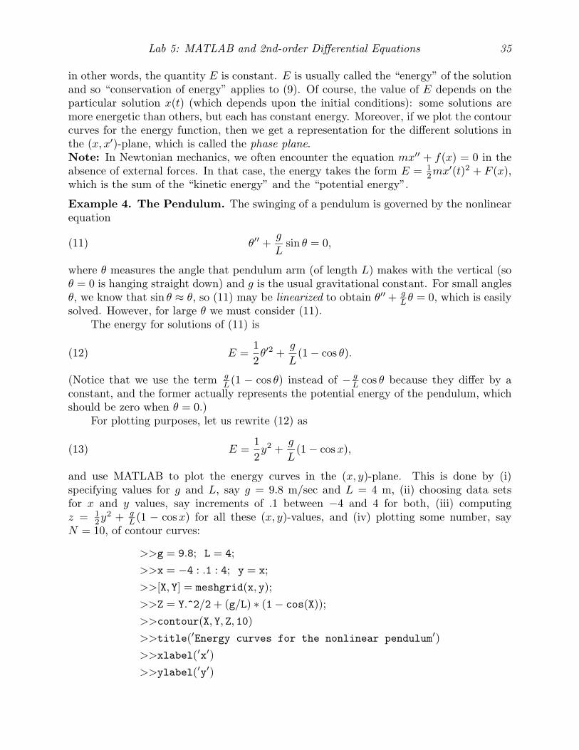
Example 4. The Pendulum. The swinging of a pendulum is governed by the nonlinearequation

(11) θ′′ +g

Lsin θ = 0,

where θ measures the angle that pendulum arm (of length L) makes with the vertical (soθ = 0 is hanging straight down) and g is the usual gravitational constant. For small anglesθ, we know that sin θ ≈ θ, so (11) may be linearized to obtain θ′′ + g

Lθ = 0, which is easilysolved. However, for large θ we must consider (11).

The energy for solutions of (11) is

(12) E =12θ′2 +

g

L(1 − cos θ).

(Notice that we use the term gL (1 − cos θ) instead of − g

L cos θ because they differ by aconstant, and the former actually represents the potential energy of the pendulum, whichshould be zero when θ = 0.)

For plotting purposes, let us rewrite (12) as

(13) E =12y2 +

g

L(1 − cosx),

and use MATLAB to plot the energy curves in the (x, y)-plane. This is done by (i)specifying values for g and L, say g = 9.8 m/sec and L = 4 m, (ii) choosing data setsfor x and y values, say increments of .1 between −4 and 4 for both, (iii) computingz = 1

2y2 + g

L (1 − cosx) for all these (x, y)-values, and (iv) plotting some number, sayN = 10, of contour curves:

>>g = 9.8; L = 4;>>x = −4 : .1 : 4; y = x;>>[X, Y] = meshgrid(x, y);>>Z = Y.^2/2 + (g/L) ∗ (1− cos(X));>>contour(X, Y, Z, 10)>>title(′Energy curves for the nonlinear pendulum′)>>xlabel(′x′)>>ylabel(′y′)

-4 -3 -2 -1 0 1 2 3 4-4

-3

-2

-1

0

1

2

3

4Energy curves for the nonlinear pendulum

x


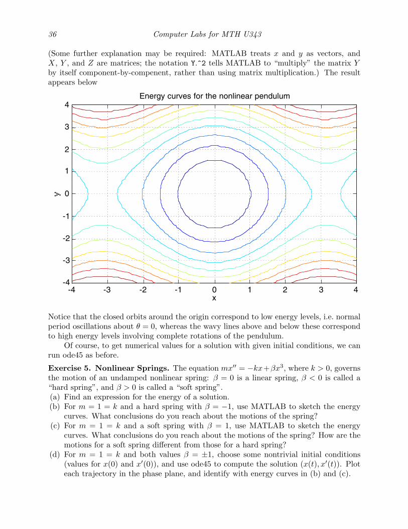
(Some further explanation may be required: MATLAB treats x and y as vectors, andX, Y , and Z are matrices; the notation Y.^2 tells MATLAB to “multiply” the matrix Yby itself component-by-compenent, rather than using matrix multiplication.) The resultappears below

Notice that the closed orbits around the origin correspond to low energy levels, i.e. normalperiod oscillations about θ = 0, whereas the wavy lines above and below these correspondto high energy levels involving complete rotations of the pendulum.

Of course, to get numerical values for a solution with given initial conditions, we canrun ode45 as before.

Exercise 5. Nonlinear Springs. The equation mx′′ = −kx+βx3, where k > 0, governsthe motion of an undamped nonlinear spring: β = 0 is a linear spring, β < 0 is called a“hard spring”, and β > 0 is called a “soft spring”.(a) Find an expression for the energy of a solution.(b) For m = 1 = k and a hard spring with β = −1, use MATLAB to sketch the energy

curves. What conclusions do you reach about the motions of the spring?(c) For m = 1 = k and a soft spring with β = 1, use MATLAB to sketch the energy

curves. What conclusions do you reach about the motions of the spring? How are themotions for a soft spring different from those for a hard spring?

(d) For m = 1 = k and both values β = ±1, choose some nontrivial initial conditions(values for x(0) and x′(0)), and use ode45 to compute the solution (x(t), x′(t)). Ploteach trajectory in the phase plane, and identify with energy curves in (b) and (c).

Documents

Computer Labs for MTH U343 Spring 2004 Textbook ... · Computer Labs for MTH U343 Spring 2004 Textbook: DiﬀerentialEquations and Linear Algebra by Edwards & Penney Contents Lab