Philipp Slusallek

Computer Graphics

- Rasterization -

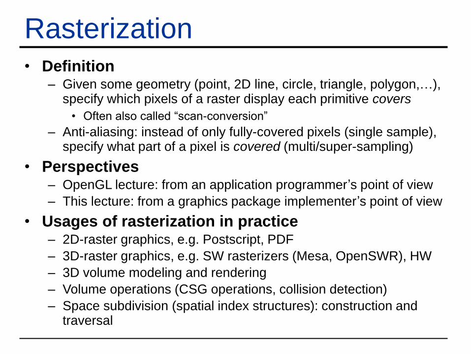
Rasterization• Definition

– Given some geometry (point, 2D line, circle, triangle, polygon,…), specify which pixels of a raster display each primitive covers

• Often also called “scan-conversion”

– Anti-aliasing: instead of only fully-covered pixels (single sample), specify what part of a pixel is covered (multi/super-sampling)

• Perspectives– OpenGL lecture: from an application programmer’s point of view

– This lecture: from a graphics package implementer’s point of view

• Usages of rasterization in practice– 2D-raster graphics, e.g. Postscript, PDF

– 3D-raster graphics, e.g. SW rasterizers (Mesa, OpenSWR), HW

– 3D volume modeling and rendering

– Volume operations (CSG operations, collision detection)

– Space subdivision (spatial index structures): construction and traversal

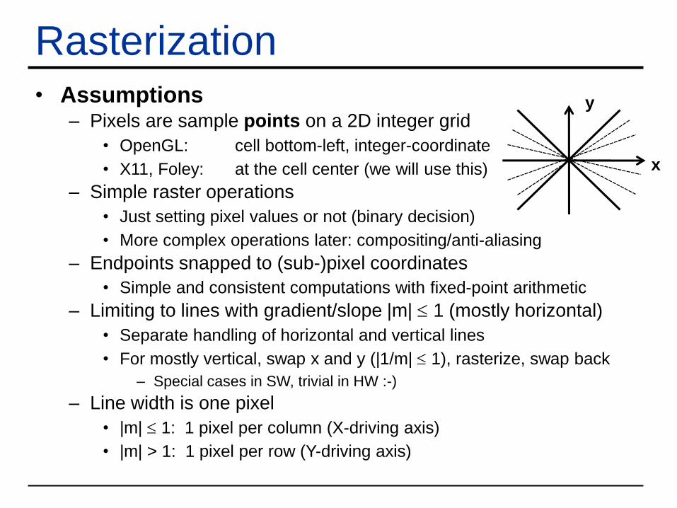
Rasterization• Assumptions

– Pixels are sample points on a 2D integer grid

• OpenGL: cell bottom-left, integer-coordinate

• X11, Foley: at the cell center (we will use this)

– Simple raster operations

• Just setting pixel values or not (binary decision)

• More complex operations later: compositing/anti-aliasing

– Endpoints snapped to (sub-)pixel coordinates

• Simple and consistent computations with fixed-point arithmetic

– Limiting to lines with gradient/slope |m| 1 (mostly horizontal)

• Separate handling of horizontal and vertical lines

• For mostly vertical, swap x and y (|1/m| 1), rasterize, swap back

– Special cases in SW, trivial in HW :-)

– Line width is one pixel

• |m| 1: 1 pixel per column (X-driving axis)

• |m| > 1: 1 pixel per row (Y-driving axis)

x

y

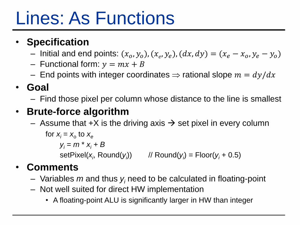
Lines: As Functions• Specification

– Initial and end points: (𝑥𝑜, 𝑦𝑜), (𝑥𝑒, 𝑦𝑒), (𝑑𝑥, 𝑑𝑦) = (𝑥𝑒 − 𝑥𝑜, 𝑦𝑒 − 𝑦𝑜)

– Functional form: 𝑦 = 𝑚𝑥 + 𝐵

– End points with integer coordinates rational slope 𝑚 = 𝑑𝑦/𝑑𝑥

• Goal– Find those pixel per column whose distance to the line is smallest

• Brute-force algorithm– Assume that +X is the driving axis set pixel in every column

for xi = xo to xe

yi = m * xi + B

setPixel(xi, Round(yi)) // Round(yi) = Floor(yi + 0.5)

• Comments– Variables m and thus yi need to be calculated in floating-point

– Not well suited for direct HW implementation

• A floating-point ALU is significantly larger in HW than integer

Lines: DDA• DDA: Digital Differential Analyzer

– Origin of incremental solvers for simple differential equations• The Euler method

– Per time-step: x’ = x + dx/dt, y’ = y + dy /dt

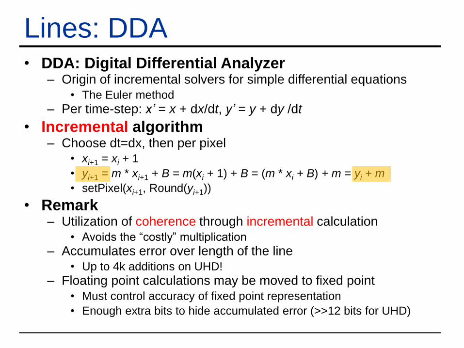
• Incremental algorithm– Choose dt=dx, then per pixel

• xi+1 = xi + 1

• yi+1 = m * xi+1 + B = m(xi + 1) + B = (m * xi + B) + m = yi + m

• setPixel(xi+1, Round(yi+1))

• Remark– Utilization of coherence through incremental calculation

• Avoids the “costly” multiplication

– Accumulates error over length of the line• Up to 4k additions on UHD!

– Floating point calculations may be moved to fixed point• Must control accuracy of fixed point representation

• Enough extra bits to hide accumulated error (>>12 bits for UHD)

Lines: Bresenham (1963)• DDA analysis

– Critical point: decision whether rounding up or down

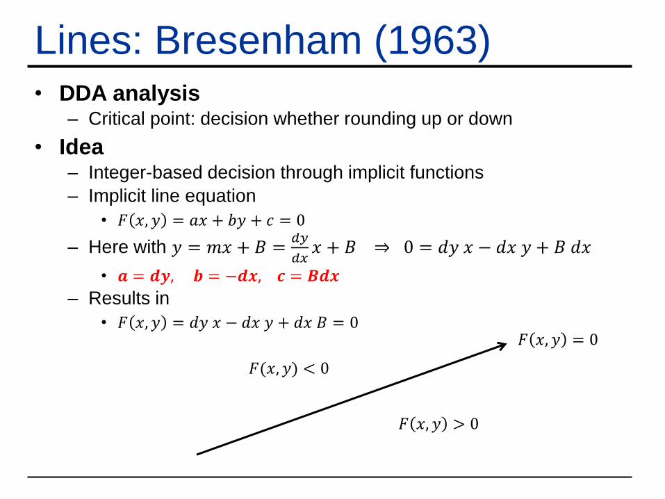
• Idea– Integer-based decision through implicit functions

– Implicit line equation

• 𝐹 𝑥, 𝑦 = 𝑎𝑥 + 𝑏𝑦 + 𝑐 = 0

– Here with 𝑦 = 𝑚𝑥 + 𝐵 =𝑑𝑦

𝑑𝑥𝑥 + 𝐵 ⇒ 0 = 𝑑𝑦 𝑥 − 𝑑𝑥 𝑦 + 𝐵 𝑑𝑥

• 𝒂 = 𝒅𝒚, 𝒃 = −𝒅𝒙, 𝒄 = 𝑩𝒅𝒙

– Results in

• 𝐹 𝑥, 𝑦 = 𝑑𝑦 𝑥 − 𝑑𝑥 𝑦 + 𝑑𝑥 𝐵 = 0𝐹 𝑥, 𝑦 = 0

𝐹 𝑥, 𝑦 > 0

𝐹(𝑥, 𝑦) < 0

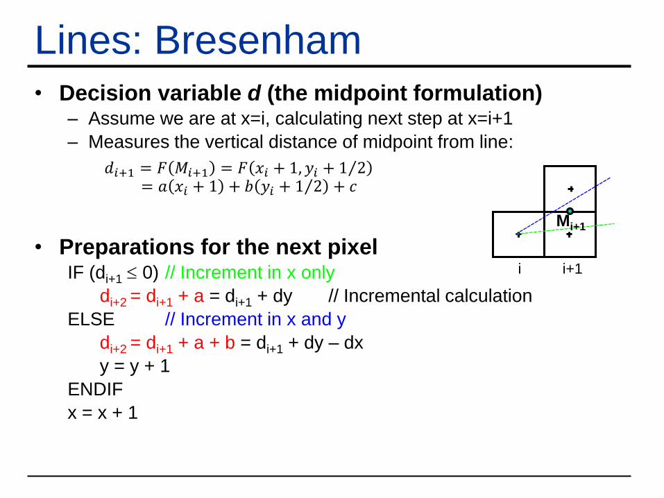
Lines: Bresenham• Decision variable d (the midpoint formulation)

– Assume we are at x=i, calculating next step at x=i+1

– Measures the vertical distance of midpoint from line:

• Preparations for the next pixelIF (di+1 0) // Increment in x only

di+2 = di+1 + a = di+1 + dy // Incremental calculation

ELSE // Increment in x and y

di+2 = di+1 + a + b = di+1 + dy – dx

y = y + 1

ENDIF

x = x + 1

𝑑𝑖+1 = 𝐹 𝑀𝑖+1 = 𝐹 𝑥𝑖 + 1, 𝑦𝑖 + 1 2= 𝑎 𝑥𝑖 + 1 + 𝑏 𝑦𝑖 + 1 2 + 𝑐

Mi+1

i i+1

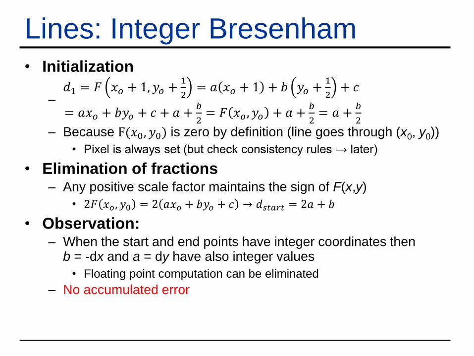
Lines: Integer Bresenham• Initialization

–𝑑1 = 𝐹 𝑥𝑜 + 1, 𝑦𝑜 +

1

2= 𝑎 𝑥𝑜 + 1 + 𝑏 𝑦𝑜 +

1

2+ 𝑐

= 𝑎𝑥𝑜 + 𝑏𝑦𝑜 + 𝑐 + 𝑎 +𝑏

2= 𝐹 𝑥𝑜, 𝑦𝑜 + 𝑎 +

𝑏

2= 𝑎 +

𝑏

2

– Because F(𝑥0, 𝑦0) is zero by definition (line goes through (x0, y0))

• Pixel is always set (but check consistency rules → later)

• Elimination of fractions– Any positive scale factor maintains the sign of F(x,y)

• 2𝐹 𝑥𝑜, 𝑦0 = 2 𝑎𝑥𝑜 + 𝑏𝑦𝑜 + 𝑐 → 𝑑𝑠𝑡𝑎𝑟𝑡 = 2𝑎 + 𝑏

• Observation:– When the start and end points have integer coordinates then

b = -dx and a = dy have also integer values

• Floating point computation can be eliminated

– No accumulated error

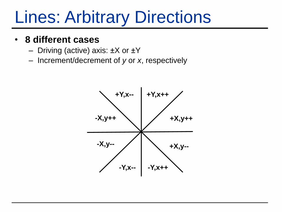
Lines: Arbitrary Directions• 8 different cases

– Driving (active) axis: ±X or ±Y

– Increment/decrement of y or x, respectively

+Y,x+++Y,x--

-Y,x-- -Y,x++

+X,y--

+X,y++-X,y++

-X,y--

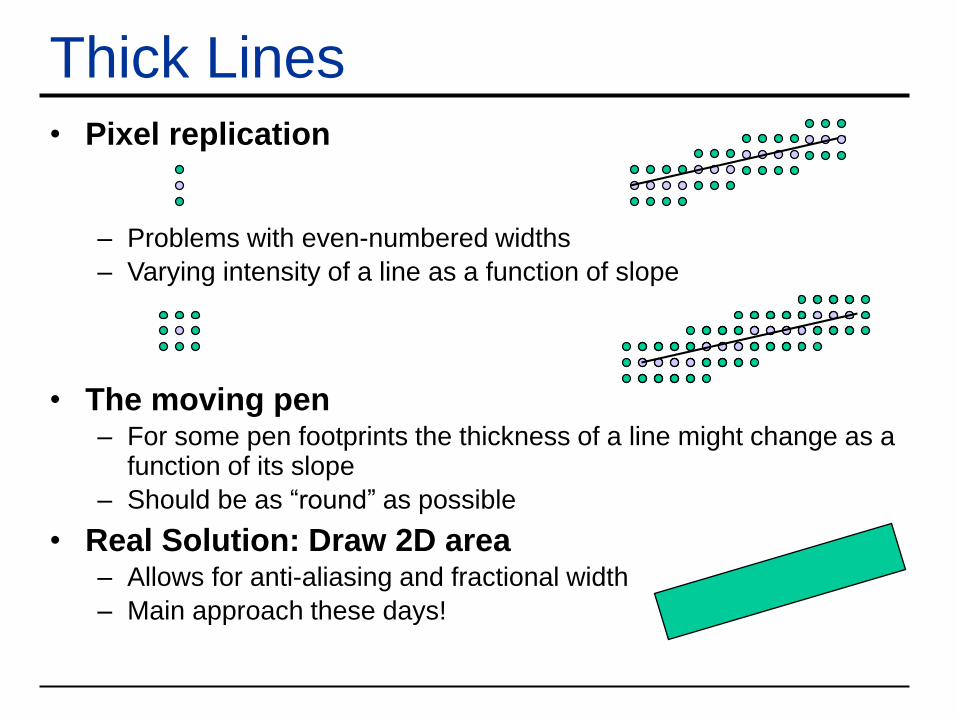
• Pixel replication

– Problems with even-numbered widths

– Varying intensity of a line as a function of slope

• The moving pen– For some pen footprints the thickness of a line might change as a

function of its slope

– Should be as “round” as possible

• Real Solution: Draw 2D area– Allows for anti-aliasing and fractional width

– Main approach these days!

Thick Lines

Handling Start and End Points• End points handling (not available in current OpenGL)

– Joining: handling of joints between lines

• Bevel: connect outer edges by straight line

• Miter: join by extending outer edges to intersection

• Round: join with radius of half the line width

– Capping: handling of end point

• Butt: end line orthogonally at end point

• Square: end line with oriented square

• Round: end line with radius of half the line width

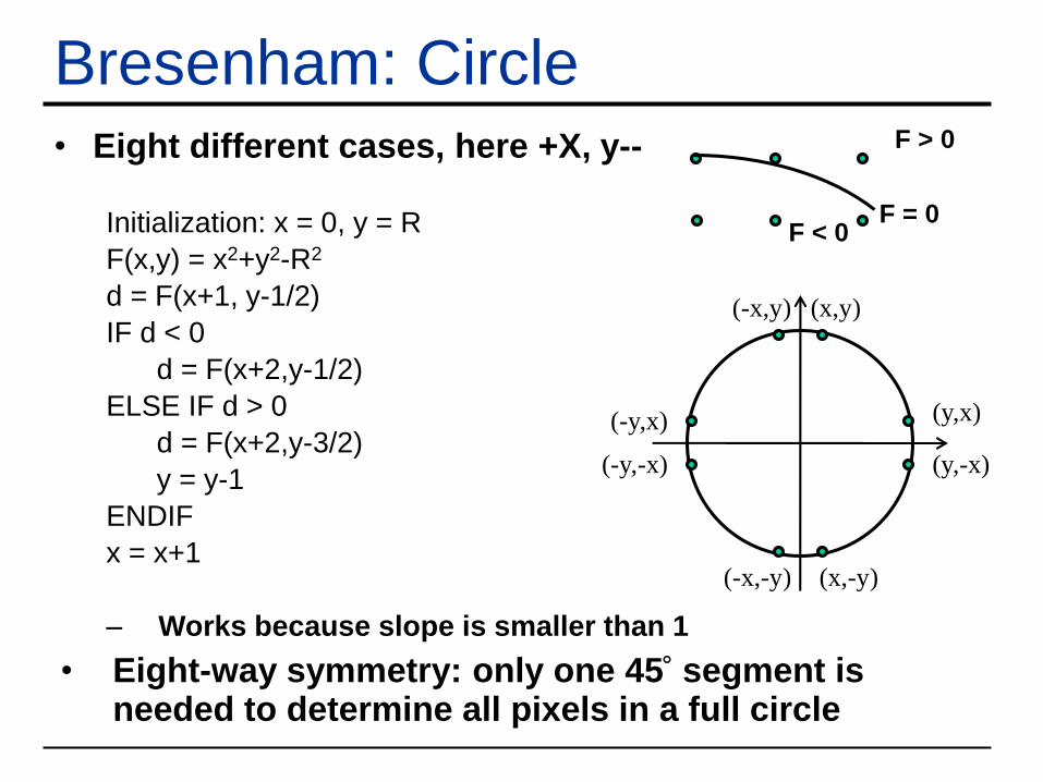
Bresenham: Circle• Eight different cases, here +X, y--

Initialization: x = 0, y = R

F(x,y) = x2+y2-R2

d = F(x+1, y-1/2)

IF d < 0

d = F(x+2,y-1/2)

ELSE IF d > 0

d = F(x+2,y-3/2)

y = y-1

ENDIF

x = x+1

– Works because slope is smaller than 1

• Eight-way symmetry: only one 45 segment is needed to determine all pixels in a full circle

F < 0

F > 0

F = 0

(x,y)

(x,-y)

(y,x)

(-x,y)

(y,-x)

(-x,-y)

(-y,x)

(-y,-x)

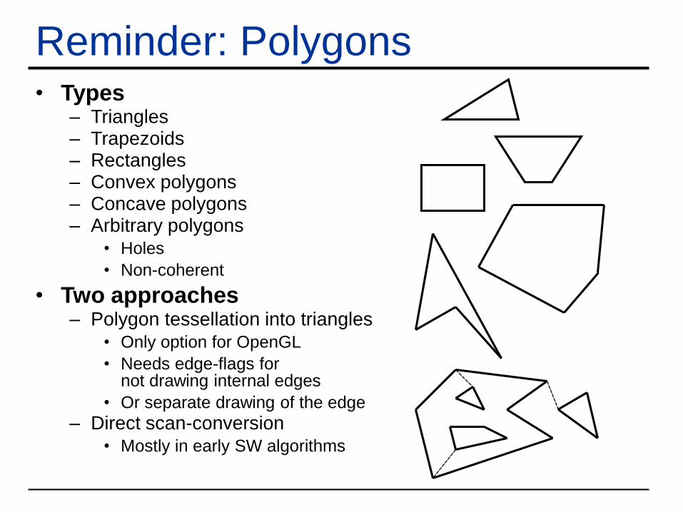
• Types– Triangles– Trapezoids– Rectangles– Convex polygons– Concave polygons– Arbitrary polygons

• Holes

• Non-coherent

• Two approaches– Polygon tessellation into triangles

• Only option for OpenGL

• Needs edge-flags fornot drawing internal edges

• Or separate drawing of the edge

– Direct scan-conversion• Mostly in early SW algorithms

Reminder: Polygons

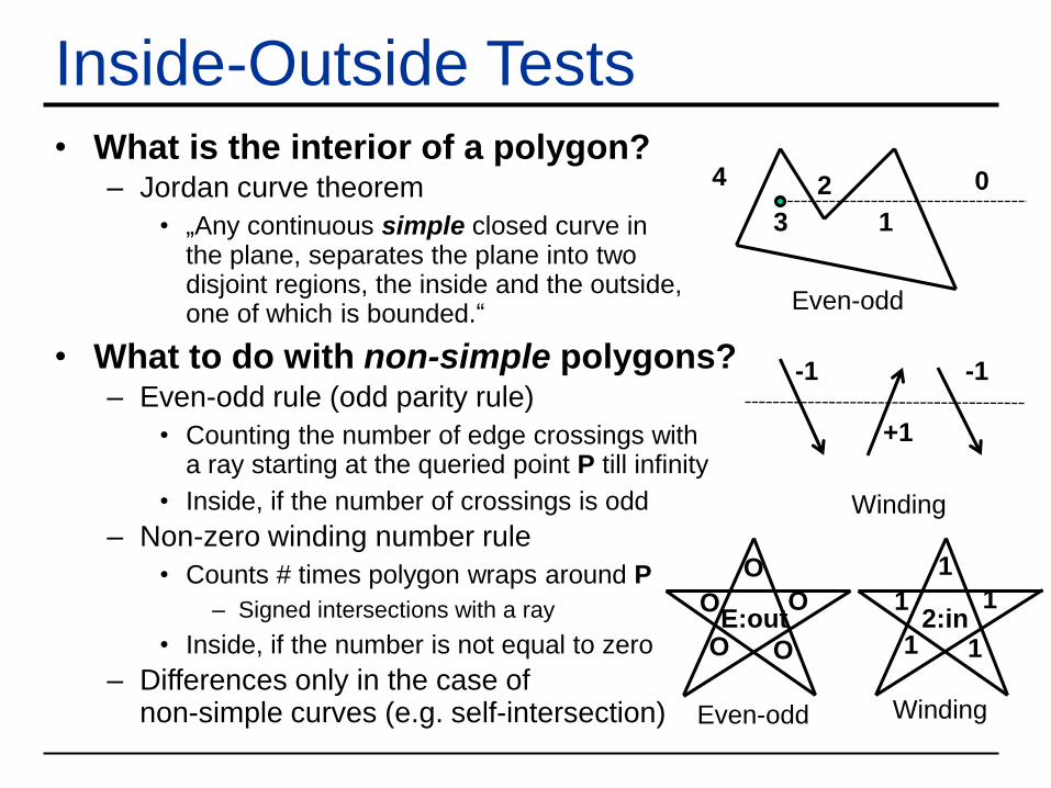
Inside-Outside Tests• What is the interior of a polygon?

– Jordan curve theorem

• „Any continuous simple closed curve inthe plane, separates the plane into twodisjoint regions, the inside and the outside,one of which is bounded.“

• What to do with non-simple polygons?– Even-odd rule (odd parity rule)

• Counting the number of edge crossings witha ray starting at the queried point P till infinity

• Inside, if the number of crossings is odd

– Non-zero winding number rule

• Counts # times polygon wraps around P

– Signed intersections with a ray

• Inside, if the number is not equal to zero

– Differences only in the case ofnon-simple curves (e.g. self-intersection)

0

1

2

3

4

-1

+1

-1

OE:out

O

O

O

1

1 1

1

1

2:inO

Even-odd Winding

Winding

Even-odd

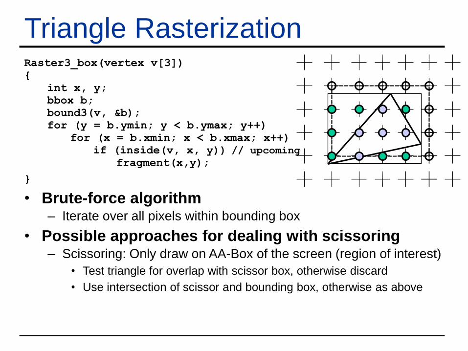
Triangle RasterizationRaster3_box(vertex v[3])

{

int x, y;

bbox b;

bound3(v, &b);

for (y = b.ymin; y < b.ymax; y++)

for (x = b.xmin; x < b.xmax; x++)

if (inside(v, x, y)) // upcoming

fragment(x,y);

}

• Brute-force algorithm– Iterate over all pixels within bounding box

• Possible approaches for dealing with scissoring– Scissoring: Only draw on AA-Box of the screen (region of interest)

• Test triangle for overlap with scissor box, otherwise discard

• Use intersection of scissor and bounding box, otherwise as above

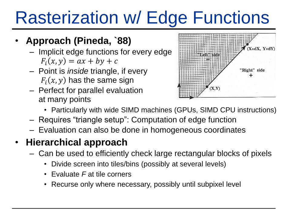
Rasterization w/ Edge Functions• Approach (Pineda, `88)

– Implicit edge functions for every edge𝐹𝑖 𝑥, 𝑦 = 𝑎𝑥 + 𝑏𝑦 + 𝑐

– Point is inside triangle, if every𝐹𝑖 𝑥, 𝑦 has the same sign

– Perfect for parallel evaluationat many points

• Particularly with wide SIMD machines (GPUs, SIMD CPU instructions)

– Requires “triangle setup”: Computation of edge function

– Evaluation can also be done in homogeneous coordinates

• Hierarchical approach– Can be used to efficiently check large rectangular blocks of pixels

• Divide screen into tiles/bins (possibly at several levels)

• Evaluate F at tile corners

• Recurse only where necessary, possibly until subpixel level

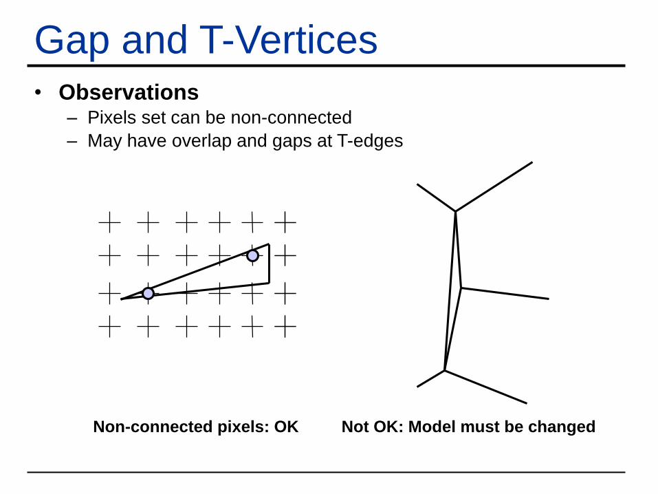
Gap and T-Vertices• Observations

– Pixels set can be non-connected

– May have overlap and gaps at T-edges

Non-connected pixels: OK Not OK: Model must be changed

Problem on Edges• Consistency: edge singularity (shared by 2 triangles)

– What if term d = ax+by+c = 0 (pixel centers lies exactly on the line)

– For d <= 0: pixels would get set twice

• Problem with some algorithms

• Transparency, XOR, CSG, ...

– Missing pixels for d < 0 (set by no tri.)

• Solution: “shadow” test– Pixels are not drawn on the right and bottom edges

– Pixels are drawn on the left and upper edges

• Evaluated via derivatives a and b

– Test for all edges also solves problem at verticesinside(value d, value a, value b)

{ // ax + by + c = 0

return (d < 0) || (d == 0 && !shadow(a, b));

}

shadow(value a, value b)

{

return (a > 0) || (a == 0 && b > 0);

}

Ray Tracing vs. Rasterization• In-Triangle test (for common origin)

– Rasterization:

• Project to 2D, clip

• Set up 2D edge functions, evaluate for each sample (using 2D point)

– Ray tracing:

• Set up 3D edge functions, evaluate for each sample (using direction)

– The ray tracing test can also be used for rasterization in 3D

• Avoids projection & clipping

• Enumerating scene primitives– Rasterization (simple):

• Linearly test them all in random order

– Rasterization (advanced):

• Build (coarse) spatial index (typically on application side)

• Traverse with (large) view frustum

– Every one separately when using tiled rendering

– Ray Tracing:

• Build (detailed) spatial index

• Traverse with (infinitely thin) ray or with some (small) frustum

– Both approaches can benefit greatly from spatial index

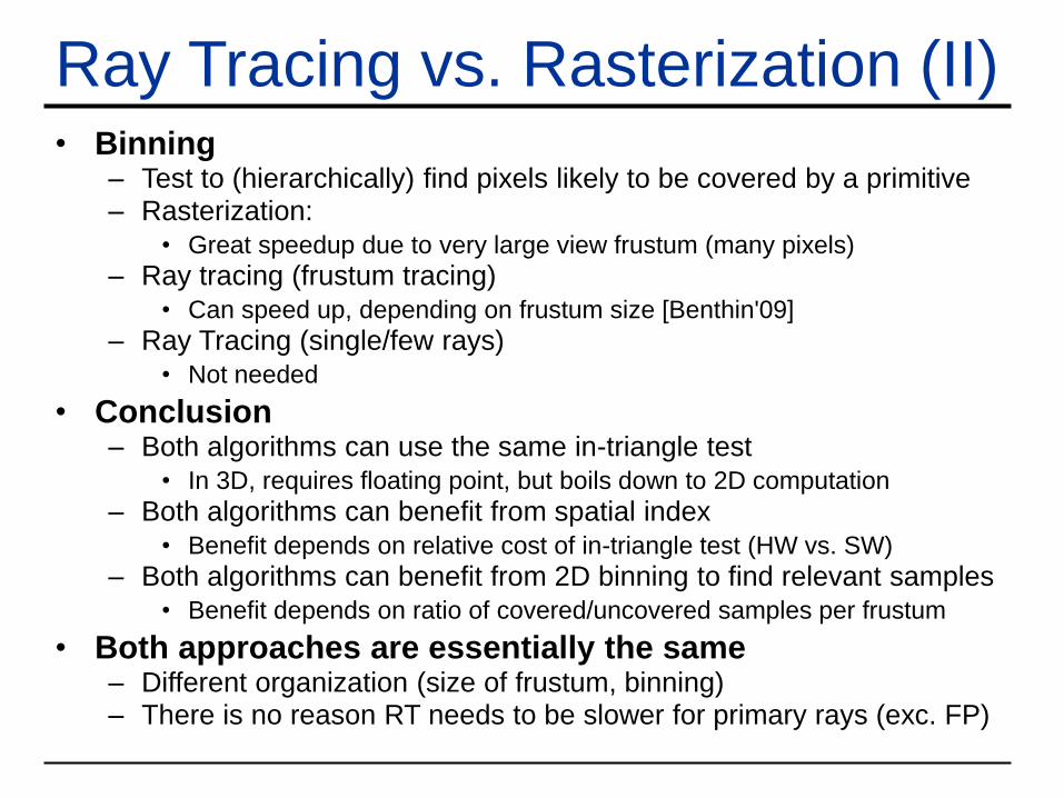
Ray Tracing vs. Rasterization (II)• Binning

– Test to (hierarchically) find pixels likely to be covered by a primitive– Rasterization:

• Great speedup due to very large view frustum (many pixels)

– Ray tracing (frustum tracing)

• Can speed up, depending on frustum size [Benthin'09]

– Ray Tracing (single/few rays)

• Not needed

• Conclusion– Both algorithms can use the same in-triangle test

• In 3D, requires floating point, but boils down to 2D computation

– Both algorithms can benefit from spatial index

• Benefit depends on relative cost of in-triangle test (HW vs. SW)

– Both algorithms can benefit from 2D binning to find relevant samples

• Benefit depends on ratio of covered/uncovered samples per frustum

• Both approaches are essentially the same– Different organization (size of frustum, binning)– There is no reason RT needs to be slower for primary rays (exc. FP)

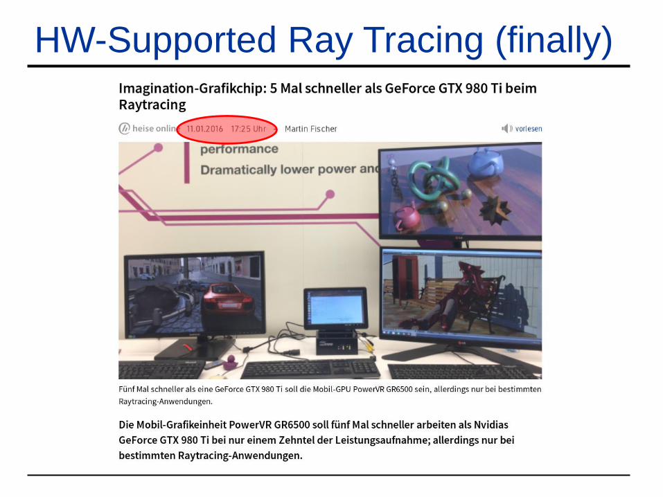
HW-Supported Ray Tracing (finally)