Computer Graphics Prof. Sukhendu Das Dept. of …textofvideo.nptel.ac.in/106106090/lec10.pdfSo we are basically projecting on to a two dimensional plane which is the screen and this

Computer Graphics Prof. Sukhendu Das

Dept. of Computer Science and Engineering Indian Institute of Technology, Madras

Lecture - 10 Three Dimensional Graphics

Welcome back to the discussion on three dimensional transformations in the course on Computer Graphics. In the last two hours we have discussed various types of transformations in three dimensions notably rotation, reflection, translation, scale and shear. And then of course we have moved towards the projective transformation that is orthographic and perspective projections. (Refer Slide Time: 00:03:59)

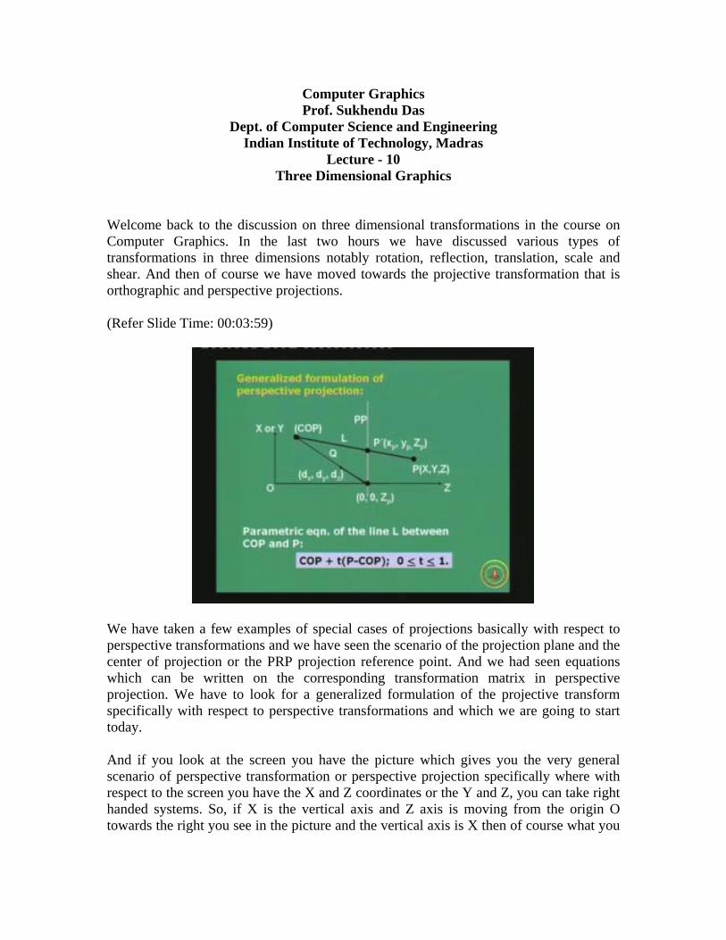
We have taken a few examples of special cases of projections basically with respect to perspective transformations and we have seen the scenario of the projection plane and the center of projection or the PRP projection reference point. And we had seen equations which can be written on the corresponding transformation matrix in perspective projection. We have to look for a generalized formulation of the projective transform specifically with respect to perspective transformations and which we are going to start today. And if you look at the screen you have the picture which gives you the very general scenario of perspective transformation or perspective projection specifically where with respect to the screen you have the X and Z coordinates or the Y and Z, you can take right handed systems. So, if X is the vertical axis and Z axis is moving from the origin O towards the right you see in the picture and the vertical axis is X then of course what you

will have is the Y axis which will basically point towards you. And of course if you similarly take the Y axis to be vertical then the X axis will point towards you. So we are basically projecting on to a two dimensional plane which is the screen and this entire three dimensional picture is what you have to view. And the projection plane, PP is the projection plane which is perpendicular to the Z axis, the normal to the projection plane is now the Z axis itself and the projection plane is also along the X-y plane. And since we are looking into X-Z plane both the X-y plane and the projection plane will appear as only lines to us Now we have assumed that the projection plane is at a Z distance Zp with respect to the origin along the Z axis, that is the distance from the origin to the point of intersection of projection plane and Z axis is Zp, so the coordinates is (0, 0, Zp) as given in the bottom of the picture. And the center of projection or the COP is along a direction vector given by (dx dy dz) respectively. These are the direction cosines of a vector from the point (0, 0, Zp) towards COP. And the COP is at a distance Q from the point (0, 0, Zp) and that is the intersection of Z axis and projection plane. Actually you can define a point anywhere in space with respect to any other point provided the direction cosines of the line joining them and the distance are known. So the distance between COP and (0, 0, Zp) is Q and the direction cosines of the vector pointing towards COP from the (0 0 Zp) point is (dx dy dz) as given in the screen. And the projection has to be taken for a point P X Y Z on the right hand side of your screen. This is the point in 3D for which the projection has to be taken. So the projector ray or the projective ray from point P to COP forms a line L. And that line L will intersect the projection plane or the PP plane at a point say P prime given by the coordinates Xp Yp and capital Zp. This Zp is the same as (0, 0, Zp) because the projection plane is at a distance Zp from the origin towards the Z axis. So the problem lies that given Q, given (dx dy dz) and given Zp we have to obtain the coordinates Xp Yp, Xy coordinates of the projected point P prime on the projection plane which is basically the projection of the point X Y Z coordinate the projection point P with coordinates X Y Z. So what are the input parameters of the algorithm? X Y Z coordinates of the point P Zp (dx dy dz) and Q. All these are given to you and the unknown quantity is Xp Yp which is nothing but the XY coordinates of the projection point P prime. So this is the picture which explains the generalized formulation or the problem of generalized formulation of perspective projection. And if you are not used to the equation of line in parametric form which is being introduced today for the first time in this course we will keep on getting this many times as we keep going along. The parametric equation of the line between COP and P is given as COP plus t times P minus COP this is a vector form of this equation where the parameter of the line t where is in the range only between 0 and 1. That means if you substitute t is equal to 0 you are basically talking of a point COP and if you take t is equal to 1 you have reach the point p. So as you vary t from 0 to 1 you are moving over the line L from COP to the point P.

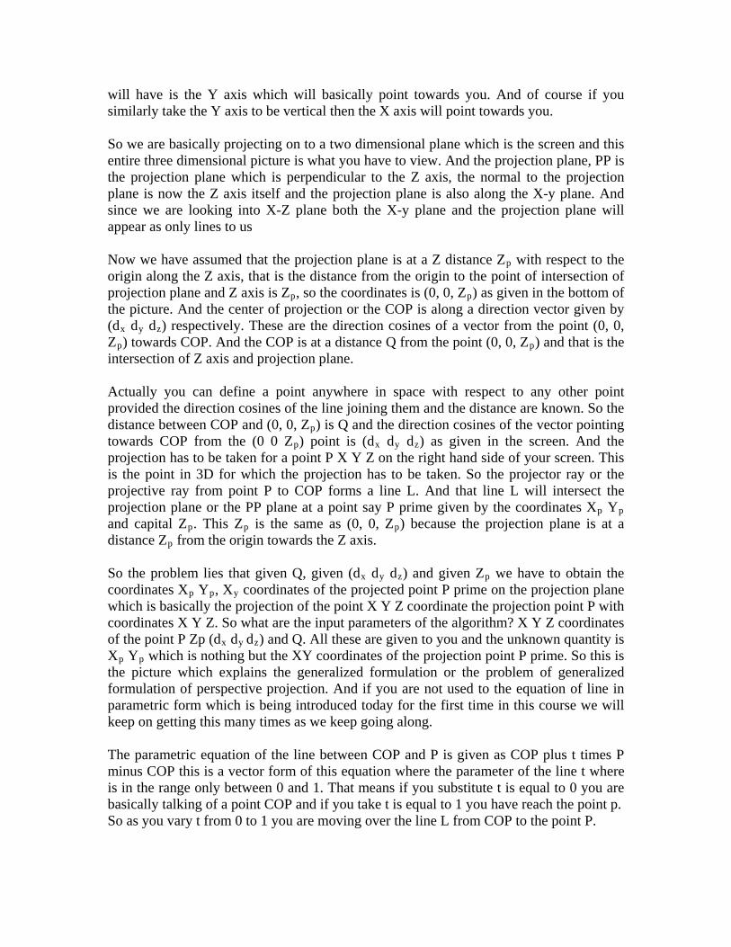
So at point P on the line L your t is equal to 1 and at the COP on the line L which is the other extreme, the parameter t is equal to 0. Any other point on the line L which lies between COP and the point P you have the values in the range 0 to 1. Let us look at how you derive the parameter t when the line L basically intersects the projection plane PP at a point P prime. And if you can somewhat get the parameter t since the coordinates of the point P and COP are known to us, if you substitute the t exactly you will get the coordinates of point P prime. The only information which is known to us is that the z coordinates of the point P prime is Zp. So look at this slide as we go along. The direction as I was telling you, the direction vector from the point (0, 0, Zp) which is the intersection of projection plane and the z axis is (0, 0, Zp). And the direction vector from that point (0, 0, Zp) to the center of projection or COP be the direction cosines given as (dx dy dz) and cube with the distance from (0, 0, Zp) to COP. (Refer Slide Time: 00:10:31)

So I can express COP also as a vector addition of (0, 0, Zp) plus Q which is the distance multiplied by dx dy dx. If you have noted down figure 1 I hope you have copied the figure, I will display the figure once again. So I am expressing COP as a vector which is (0, 0, Zp) plus the Q vector multiplied by the direction cosines (dx dy dz) where Q is a scalar quantity so that is how COP is expressed here. So we will keep going back and forth to the figure and come back here if necessary. So the coordinates of any point on line L can be given as X prime Y prime Z prime as Q dx plus X minus Q dx times t and similarly Y prime and similarly Z prime. How do you get this? You get this basically because when we go back to the figure you have seen the expression of the line L and the COP is now known. We have defined COP as (0, 0, Zp) vector plus Q times (dx dy dz) and P is known. Therefore, using this information with little bit of mathematical manipulation here you can actually find the

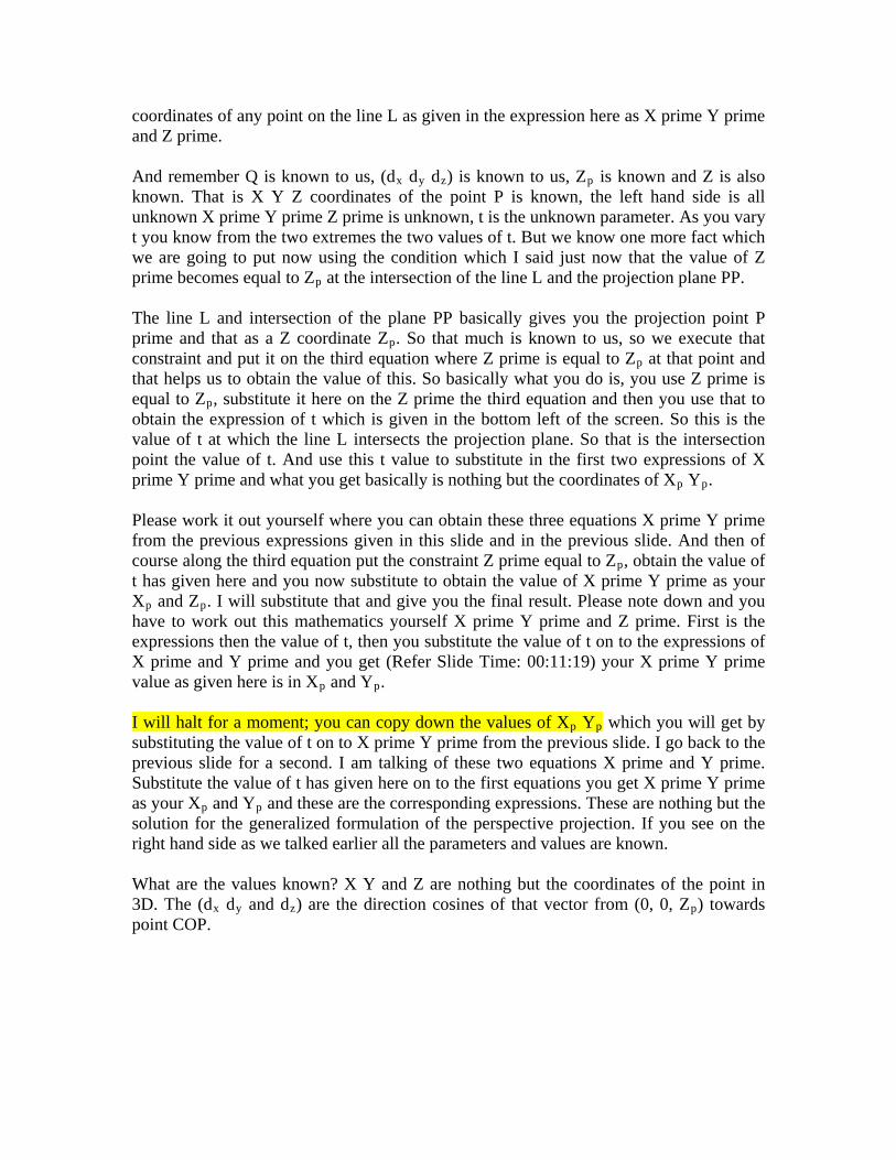
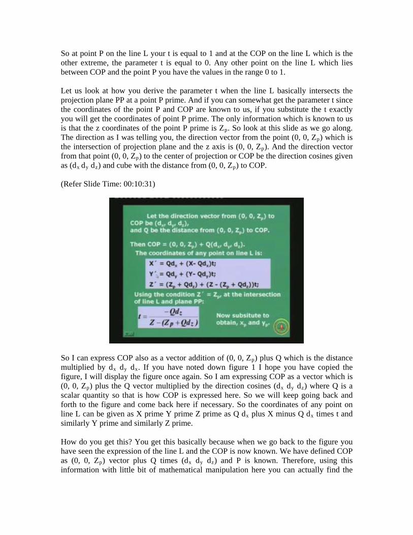
coordinates of any point on the line L as given in the expression here as X prime Y prime and Z prime. And remember Q is known to us, (dx dy dz) is known to us, Zp is known and Z is also known. That is X Y Z coordinates of the point P is known, the left hand side is all unknown X prime Y prime Z prime is unknown, t is the unknown parameter. As you vary t you know from the two extremes the two values of t. But we know one more fact which we are going to put now using the condition which I said just now that the value of Z prime becomes equal to Zp at the intersection of the line L and the projection plane PP. The line L and intersection of the plane PP basically gives you the projection point P prime and that as a Z coordinate Zp. So that much is known to us, so we execute that constraint and put it on the third equation where Z prime is equal to Zp at that point and that helps us to obtain the value of this. So basically what you do is, you use Z prime is equal to Zp, substitute it here on the Z prime the third equation and then you use that to obtain the expression of t which is given in the bottom left of the screen. So this is the value of t at which the line L intersects the projection plane. So that is the intersection point the value of t. And use this t value to substitute in the first two expressions of X prime Y prime and what you get basically is nothing but the coordinates of Xp Yp. Please work it out yourself where you can obtain these three equations X prime Y prime from the previous expressions given in this slide and in the previous slide. And then of course along the third equation put the constraint Z prime equal to Zp, obtain the value of t has given here and you now substitute to obtain the value of X prime Y prime as your Xp and Zp. I will substitute that and give you the final result. Please note down and you have to work out this mathematics yourself X prime Y prime and Z prime. First is the expressions then the value of t, then you substitute the value of t on to the expressions of X prime and Y prime and you get (Refer Slide Time: 00:11:19) your X prime Y prime value as given here is in Xp and Yp. I will halt for a moment; you can copy down the values of Xp Yp which you will get by substituting the value of t on to X prime Y prime from the previous slide. I go back to the previous slide for a second. I am talking of these two equations X prime and Y prime. Substitute the value of t has given here on to the first equations you get X prime Y prime as your Xp and Yp and these are the corresponding expressions. These are nothing but the solution for the generalized formulation of the perspective projection. If you see on the right hand side as we talked earlier all the parameters and values are known. What are the values known? X Y and Z are nothing but the coordinates of the point in 3D. The (dx dy and dz) are the direction cosines of that vector from (0, 0, Zp) towards point COP.

(Refer Slide Time: 00:12:53)

And of course you also know Zp which is the intersection of the distance of the projection plane from the origin and that is the vertical distance basically Zp. And Q is also known because that is the distance of COP from the point (0, 0, Zp), so all the parameters in the right hand side are known. You can substitute and get the values of Xp Yp and those are nothing but now the values of your coordinates of the 2D projection of the point in 3D. From 3D to 2D this is the generalized formulation. When you go back to the generalized transformation matrix and use the expression as given in the previous slide of Xp and Yp you will be able to obtain you should be able to obtain the expression of the generalized transformation matrix I give this as an exercise for you, please try it. With all these expressions you have to write it out otherwise you cannot derive at it. Otherwise you will easily lose the concept and you will fail to understand the concept. So what you must do is, you must write these equations, draw the figures yourself, understand the vector equations. The parametric equation of a line is what you have to use and then from the expressions which you have got as Xp and Yp you have to get the generalized transformation matrix in general as given here. This is the form, you can please note down the values here. So P prime is M times, P where M is a transformation matrix, generalized formulation of the perspective projection matrix. And if you use this generalized formulation which will help you to obtain the 2D coordinates from the 3D points.


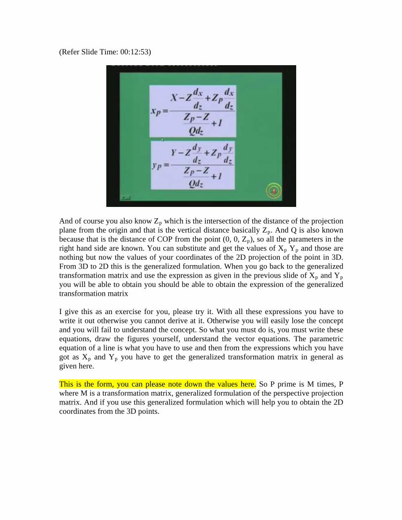
Therefore, projection of a point in 3D on to a 2D plane generalized formulation is given here by M gen. I hope you are able to copy the corresponding elements of this matrix which you should try to derive yourself. Of course all these have been borrowed from the book by Foley Van Dam binary use. We will look at some special cases from the generalized formulation of the perspective projection matrix where the matrix type can take special forms and shapes depending upon the values of Zp Q and the direction cosines (dx dy dz). The first row talks about the case when the Zp is at the origin. So you have moved the projection plane at the origin, Q is at infinity. The Q is the distance that means the center of projection has now moved to infinity. If the center of projection moves to infinity we know that the projective rays from the point towards the center of projection passing from the projection plane will all be parallel. Hence the transformation matrix will become an orthogonal matrix and hence we have written M orth that means it is a transformation matrix for orthogonal case and the direction vector (dx dy dz) will also take the form [0 0 minus 1]. [0 0 minus 1] form of (dx dy dz) is also same for the next two rows. Basically [0 0 minus 1] type of unit vector if you see is nothing but a vector which is looking towards the minus Z axis. And your view is along the positive Z axis and the direction vector from the projection plane or the plane normal towards center of projection is [0 0 minus 1].

(Refer Slide Time: 16:30)

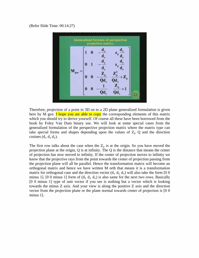
So we have understood what is M orthogonal matrix from a generalized formulation. The second one if you take, Zp equal to d that means wherever it was earlier, Q is also equal to d and the direction cosines [0 0 minus 1] we get a special case of a perspective projection matrix where my COP is at the origin now and the projection plane is at the distance d from the origin and the surface normal of the projection plane is pointing towards the minus Z axis where you get the special case of simple perspective projection matrix and we have already derived at these expressions in the previous class. A special case of M prime bar, dash is the case when Zp is equal to 0 and Q is at d. That means the projection plane is now at the origin and the center of the projection is also at the origin d and if that is the case you get M prime from. I expect you to obtain the special cases of these matrices by putting these constraints and you get them basically by substituting these conditions on the elements of this generalized matrix. Substitute them and get the special forms of the matrices, namely the types of orthogonal and perspective matrices. If you note the last point here, is of course Q is finite which is the case of perspective projection matrix when only Q becomes infinite we are talking of orthogonal otherwise when Q is finite we have perspective projection matrix. The rays converge at a point and the rays are not parallel to all. The generalized transformation matrix defines what we call as a one point perspective projection in the above two cases. Above two cases means the last two cases as given in the three different cases, special cases in the table here. I hope you still remember the one point, two point and three point perspective projection systems in perspective projection.


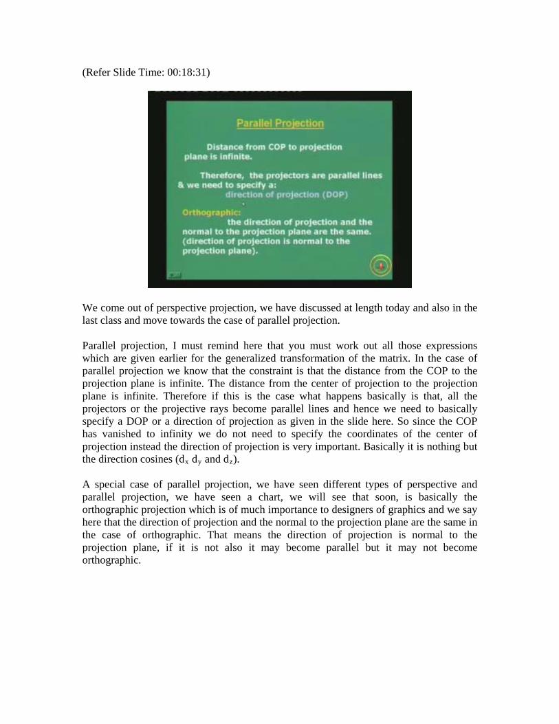
We come out of perspective projection, we have discussed at length today and also in the last class and move towards the case of parallel projection. Parallel projection, I must remind here that you must work out all those expressions which are given earlier for the generalized transformation of the matrix. In the case of parallel projection we know that the constraint is that the distance from the COP to the projection plane is infinite. The distance from the center of projection to the projection plane is infinite. Therefore if this is the case what happens basically is that, all the projectors or the projective rays become parallel lines and hence we need to basically specify a DOP or a direction of projection as given in the slide here. So since the COP has vanished to infinity we do not need to specify the coordinates of the center of projection instead the direction of projection is very important. Basically it is nothing but the direction cosines (dx dy and dz). A special case of parallel projection, we have seen different types of perspective and parallel projection, we have seen a chart, we will see that soon, is basically the orthographic projection which is of much importance to designers of graphics and we say here that the direction of projection and the normal to the projection plane are the same in the case of orthographic. That means the direction of projection is normal to the projection plane, if it is not also it may become parallel but it may not become orthographic.


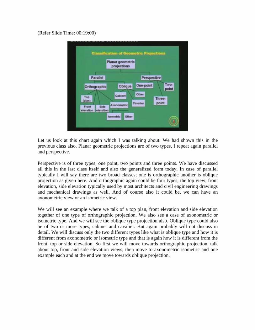
Let us look at this chart again which I was talking about. We had shown this in the previous class also. Planar geometric projections are of two types, I repeat again parallel and perspective. Perspective is of three types; one point, two points and three points. We have discussed all this in the last class itself and also the generalized form today. In case of parallel typically I will say there are two broad classes; one is orthographic another is oblique projection as given here. And orthographic again could be four types; the top view, front elevation, side elevation typically used by most architects and civil engineering drawings and mechanical drawings as well. And of course also it could be, we can have an axonometric view or an isometric view. We will see an example where we talk of a top plan, front elevation and side elevation together of one type of orthographic projection. We also see a case of axonometric or isometric type. And we will see the oblique type projection also. Oblique type could also be of two or more types, cabinet and cavalier. But again probably will not discuss in detail. We will discuss only the two different types like what is oblique type and how it is different from axonometric or isometric type and that is again how it is different from the front, top or side elevation. So first we will move towards orthographic projection, talk about top, front and side elevation views, then move to axonometric isometric and one example each and at the end we move towards oblique projection.


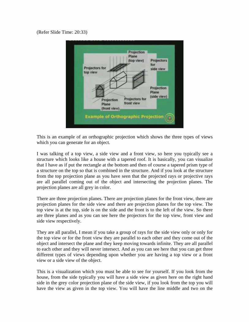
This is an example of an orthographic projection which shows the three types of views which you can generate for an object. I was talking of a top view, a side view and a front view, so here you typically see a structure which looks like a house with a tapered roof. It is basically, you can visualize that I have as if put the rectangle at the bottom and then of course a tapered prism type of a structure on the top so that is combined in the structure. And if you look at the structure from the top projection plane as you have seen that the projected rays or projective rays are all parallel coming out of the object and intersecting the projection planes. The projection planes are all grey in color. There are three projection planes. There are projection planes for the front view, there are projection planes for the side view and there are projection planes for the top view. The top view is at the top, side is on the side and the front is to the left of the view. So there are three planes and as you can see here the projectors for the top view, front view and side view respectively. They are all parallel, I mean if you take a group of rays for the side view only or only for the top view or for the front view they are parallel to each other and they come out of the object and intersect the plane and they keep moving towards infinite. They are all parallel to each other and they will never intersect. And as you can see here that you can get three different types of views depending upon whether you are having a top view or a front view or a side view of the object. This is a visualization which you must be able to see for yourself. If you look from the house, from the side typically you will have a side view as given here on the right hand side in the grey color projection plane of the side view, if you look from the top you will have the view as given in the top view. You will have the line middle and two on the

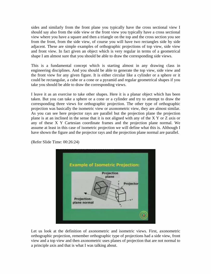
sides and similarly from the front plane you typically have the cross sectional view I should say also from the side view or the front view you typically have a cross sectional view where you have a square and then a triangle on the top and the cross section you see from the front, from the side view, of course you will have two rectangles side by side adjacent. These are simple examples of orthographic projections of top view, side view and front view. In fact given an object which is very regular in terms of a geometrical shape I am almost sure that you should be able to draw the corresponding side views. This is a fundamental concept which is starting almost in any drawing class in engineering disciplines. And you should be able to generate the top view, side view and the front view for any given figure. It is either circular like a cylinder or a sphere or it could be rectangular, a cube or a cone or a pyramid and regular geometrical shapes if you take you should be able to draw the corresponding views. I leave it as an exercise to take other shapes. Here it is a planar object which has been taken. But you can take a sphere or a cone or a cylinder and try to attempt to draw the corresponding three views for orthographic projection. The other type of orthographic projection was basically the isometric view or axonometric view, they are almost similar. As you can see here projector rays are parallel but the projection plane the projection plane is at an inclined in the sense that it is not aligned with any of the X Y or Z axis or any of these X Y Cartesian coordinate frames and the projection plane normal. We assume at least in this case of isometric projection we will define what this is. Although I have shown the figure and the projector rays and the projection plane normal are parallel. (Refer Slide Time: 00:26:24)

Let us look at the definition of axonometric and isometric views. First, axonometric orthographic projection, remember orthographic type of projections had a side view, front view and a top view and then axonometric uses planes of projection that are not normal to a principle axis and that is what I was talking about.


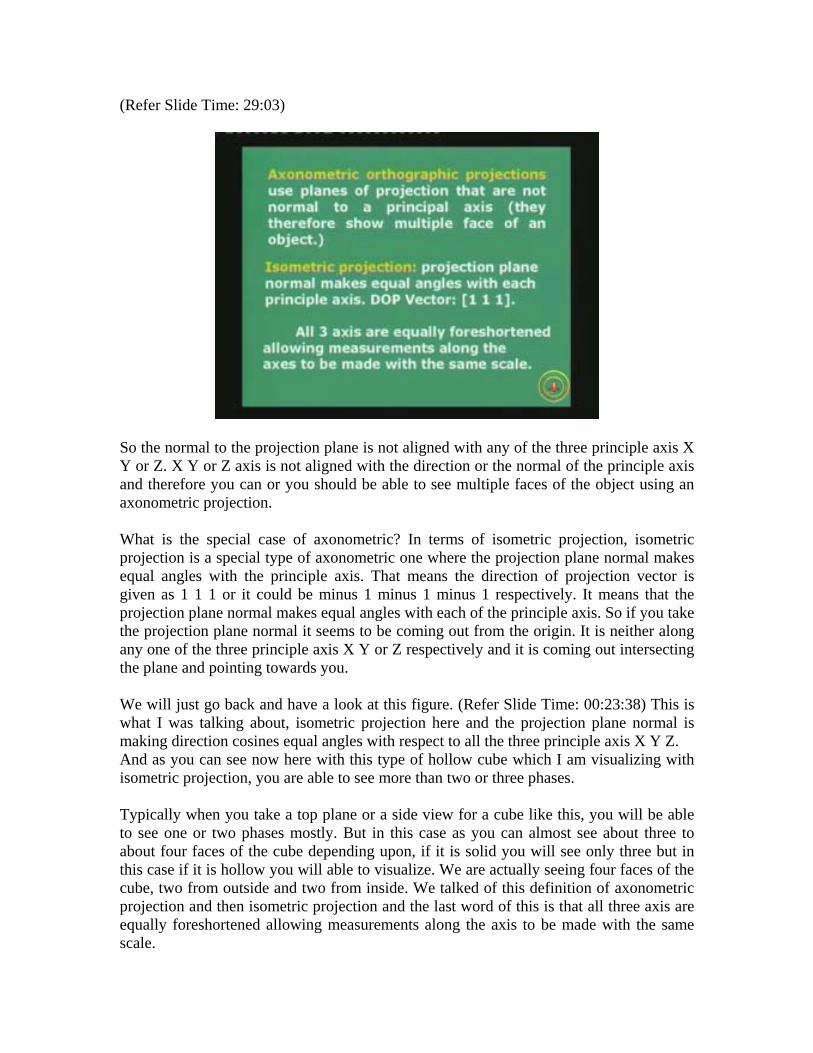
So the normal to the projection plane is not aligned with any of the three principle axis X Y or Z. X Y or Z axis is not aligned with the direction or the normal of the principle axis and therefore you can or you should be able to see multiple faces of the object using an axonometric projection. What is the special case of axonometric? In terms of isometric projection, isometric projection is a special type of axonometric one where the projection plane normal makes equal angles with the principle axis. That means the direction of projection vector is given as 1 1 1 or it could be minus 1 minus 1 minus 1 respectively. It means that the projection plane normal makes equal angles with each of the principle axis. So if you take the projection plane normal it seems to be coming out from the origin. It is neither along any one of the three principle axis X Y or Z respectively and it is coming out intersecting the plane and pointing towards you. We will just go back and have a look at this figure. (Refer Slide Time: 00:23:38) This is what I was talking about, isometric projection here and the projection plane normal is making direction cosines equal angles with respect to all the three principle axis X Y Z. And as you can see now here with this type of hollow cube which I am visualizing with isometric projection, you are able to see more than two or three phases. Typically when you take a top plane or a side view for a cube like this, you will be able to see one or two phases mostly. But in this case as you can almost see about three to about four faces of the cube depending upon, if it is solid you will see only three but in this case if it is hollow you will able to visualize. We are actually seeing four faces of the cube, two from outside and two from inside. We talked of this definition of axonometric projection and then isometric projection and the last word of this is that all three axis are equally foreshortened allowing measurements along the axis to be made with the same scale.

This is a special case of axonometric projection which is isometric where we know that the projection plane normal makes equal angles with each of the principle axis and the first criteria of the definition of axonometric projection also holds good. That means you use planes of projection that are not normal to your principle axis so you can place it anywhere in axonometric but in the special case of isometric it must make equal angles. What must make? The projection plane normal must make equal angles with the three principle axis XYZ. And typical example is the direction of projection vector which is nothing but, for this also the projection plane normal is given as 1 1 1 and all the three axis or the dimensions of the object along all three axis appear to be equal and same for the isometric projection. Oblique projection was a different type of orthographic projection. Unlike the orthographic case, orthographic had top, side plan and an axonometric and isometric as well which is a part of the isometric. (Refer Slide Time: 00:29:20)

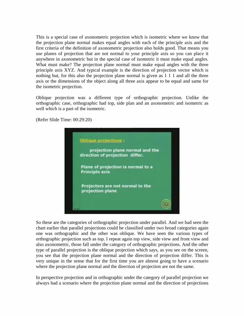
So these are the categories of orthographic projection under parallel. And we had seen the chart earlier that parallel projections could be classified under two broad categories again one was orthographic and the other was oblique. We have seen the various types of orthographic projection such as top. I repeat again top view, side view and front view and also axonometric, those fall under the category of orthographic projections. And the other type of parallel projection is the oblique projection which says, as you see on the screen, you see that the projection plane normal and the direction of projection differ. This is very unique in the sense that for the first time you are almost going to have a scenario where the projection plane normal and the direction of projection are not the same. In perspective projection and in orthographic under the category of parallel projection we always had a scenario where the projection plane normal and the direction of projections

those two vectors were the same and they coincided. But in the oblique projection, the funny case where the projector rays which usually intersect normally with the projection plane in all other types of projection models does not happen in the case of oblique. So you can take a plane and instead of projector rays parallelly intersecting the projection plane they intersect at an angle. So the plane normal and the direction of the projector rays are not parallel anymore in the case of oblique projection. We will see with an example and few more points. So plane of projection is normal to a principle axis. So we come back to the forms of the special type of orthographic projection is the top plan side etc or even perspective projection while the planer projection is now made in such a manner that it is normal to a principle axis or the projection plane normal itself is one of the principle axis. But the projectors are not normal to the projection plane. Earlier projectors were moving along the direction of the normal to the projection plane but they are not anymore. So how do we visualize this figure? Let us look at this figure. (Refer Slide Time: 00:29:31)

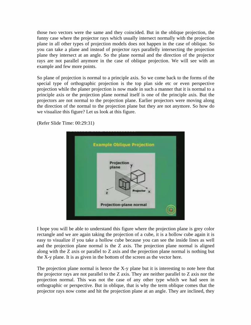
I hope you will be able to understand this figure where the projection plane is grey color rectangle and we are again taking the projection of a cube, it is a hollow cube again it is easy to visualize if you take a hollow cube because you can see the inside lines as well and the projection plane normal is the Z axis. The projection plane normal is aligned along with the Z axis or parallel to Z axis and the projection plane normal is nothing but the X-y plane. It is as given in the bottom of the screen as the vector here. The projection plane normal is hence the X-y plane but it is interesting to note here that the projector rays are not parallel to the Z axis. They are neither parallel to Z axis nor the projection normal. This was not the case of any other type which we had seen in orthographic or perspective. But in oblique, that is why the term oblique comes that the projector rays now come and hit the projection plane at an angle. They are inclined, they

are not normal, they are not parallel to the projection plane normal, they are not parallel to the Z axis but they hit on the projection plane at an inclined and this is what gives you what is called as an oblique projection. It could be useful in certain cases but difficult to typically derive expressions. But you must know the type of oblique projection as given here. (Refer Slide Time: 00:30:52)

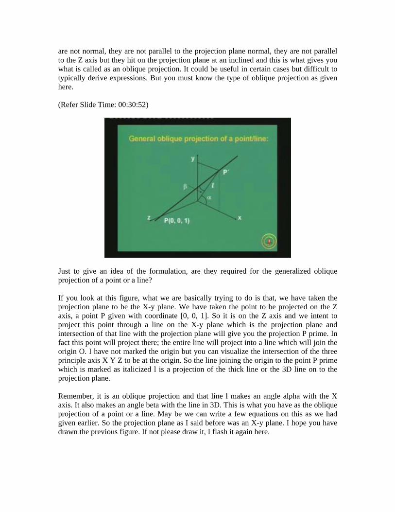
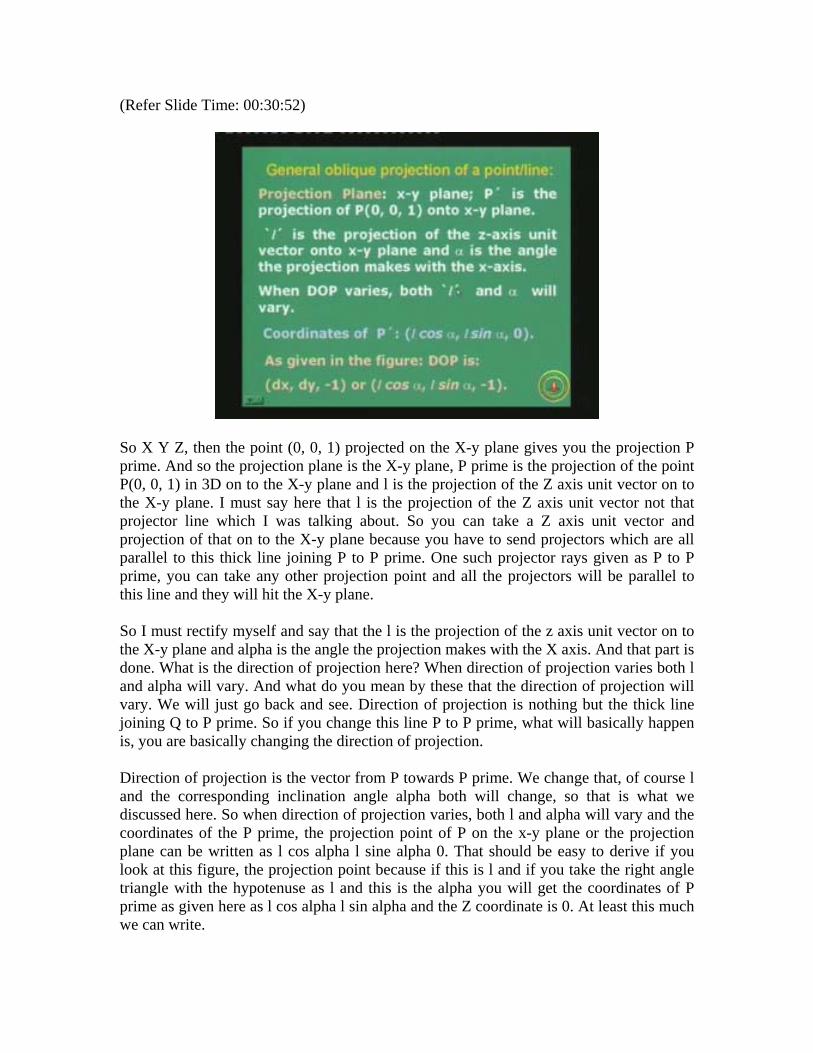
Just to give an idea of the formulation, are they required for the generalized oblique projection of a point or a line? If you look at this figure, what we are basically trying to do is that, we have taken the projection plane to be the X-y plane. We have taken the point to be projected on the Z axis, a point P given with coordinate [0, 0, 1]. So it is on the Z axis and we intent to project this point through a line on the X-y plane which is the projection plane and intersection of that line with the projection plane will give you the projection P prime. In fact this point will project there; the entire line will project into a line which will join the origin O. I have not marked the origin but you can visualize the intersection of the three principle axis X Y Z to be at the origin. So the line joining the origin to the point P prime which is marked as italicized l is a projection of the thick line or the 3D line on to the projection plane. Remember, it is an oblique projection and that line l makes an angle alpha with the X axis. It also makes an angle beta with the line in 3D. This is what you have as the oblique projection of a point or a line. May be we can write a few equations on this as we had given earlier. So the projection plane as I said before was an X-y plane. I hope you have drawn the previous figure. If not please draw it, I flash it again here.


So X Y Z, then the point (0, 0, 1) projected on the X-y plane gives you the projection P prime. And so the projection plane is the X-y plane, P prime is the projection of the point P(0, 0, 1) in 3D on to the X-y plane and l is the projection of the Z axis unit vector on to the X-y plane. I must say here that l is the projection of the Z axis unit vector not that projector line which I was talking about. So you can take a Z axis unit vector and projection of that on to the X-y plane because you have to send projectors which are all parallel to this thick line joining P to P prime. One such projector rays given as P to P prime, you can take any other projection point and all the projectors will be parallel to this line and they will hit the X-y plane. So I must rectify myself and say that the l is the projection of the z axis unit vector on to the X-y plane and alpha is the angle the projection makes with the X axis. And that part is done. What is the direction of projection here? When direction of projection varies both l and alpha will vary. And what do you mean by these that the direction of projection will vary. We will just go back and see. Direction of projection is nothing but the thick line joining Q to P prime. So if you change this line P to P prime, what will basically happen is, you are basically changing the direction of projection. Direction of projection is the vector from P towards P prime. We change that, of course l and the corresponding inclination angle alpha both will change, so that is what we discussed here. So when direction of projection varies, both l and alpha will vary and the coordinates of the P prime, the projection point of P on the x-y plane or the projection plane can be written as l cos alpha l sine alpha 0. That should be easy to derive if you look at this figure, the projection point because if this is l and if you take the right angle triangle with the hypotenuse as l and this is the alpha you will get the coordinates of P prime as given here as l cos alpha l sin alpha and the Z coordinate is 0. At least this much we can write.

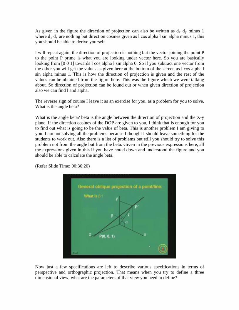
As given in the figure the direction of projection can also be written as dx dy minus 1 where dx dy are nothing but direction cosines given as l cos alpha l sin alpha minus 1, this you should be able to derive yourself. I will repeat again; the direction of projection is nothing but the vector joining the point P to the point P prime is what you are looking under vector here. So you are basically looking from [0 0 1] towards l cos alpha l sin alpha 0. So if you subtract one vector from the other you will get the values as given here at the bottom of the screen as l cos alpha l sin alpha minus 1. This is how the direction of projection is given and the rest of the values can be obtained from the figure here. This was the figure which we were talking about. So direction of projection can be found out or when given direction of projection also we can find l and alpha. The reverse sign of course I leave it as an exercise for you, as a problem for you to solve. What is the angle beta? What is the angle beta? beta is the angle between the direction of projection and the X-y plane. If the direction cosines of the DOP are given to you, I think that is enough for you to find out what is going to be the value of beta. This is another problem I am giving to you. I am not solving all the problems because I thought I should leave something for the students to work out. Also there is a list of problems but still you should try to solve this problem not from the angle but from the beta. Given in the previous expressions here, all the expressions given in this if you have noted down and understood the figure and you should be able to calculate the angle beta. (Refer Slide Time: 00:36:20)

Now just a few specifications are left to describe various specifications in terms of perspective and orthographic projection. That means when you try to define a three dimensional view, what are the parameters of that view you need to define?


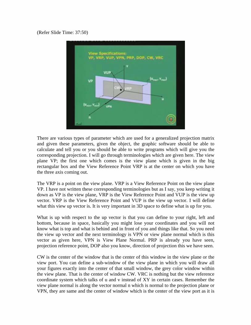
There are various types of parameter which are used for a generalized projection matrix and given these parameters, given the object, the graphic software should be able to calculate and tell you or you should be able to write programs which will give you the corresponding projection. I will go through terminologies which are given here. The view plane VP; the first one which comes is the view plane which is given in the big rectangular box and the View Reference Point VRP is at the center on which you have the three axis coming out. The VRP is a point on the view plane. VRP is a View Reference Point on the view plane VP. I have not written these corresponding terminologies but as I say, you keep writing it down as VP is the view plane, VRP is the View Reference Point and VUP is the view up vector. VRP is the View Reference Point and VUP is the view up vector. I will define what this view up vector is. It is very important in 3D space to define what is up for you. What is up with respect to the up vector is that you can define to your right, left and bottom, because in space, basically you might lose your coordinates and you will not know what is top and what is behind and in front of you and things like that. So you need the view up vector and the next terminology is VPN or view plane normal which is this vector as given here, VPN is View Plane Normal. PRP is already you have seen, projection reference point, DOP also you know, direction of projection this we have seen. CW is the center of the window that is the center of this window in the view plane or the view port. You can define a sub-window of the view plane in which you will draw all your figures exactly into the center of that small window, the grey color window within the view plane. That is the center of window CW. VRC is nothing but the view reference coordinate system which talks of u and v instead of XY in certain cases. Remember the view plane normal is along the vector normal n which is normal to the projection plane or VPN, they are same and the center of window which is the center of the view port as it is

called the small rectangle running from coordinates U min V min to a maximum of U max V max in the u v coordinates space. The UV coordinates space is defined to define the view reference coordinate systems on the view plane. So these are the terminologies. If you have missed anything I will repeat again. VP is view plane, VRP is View Reference Point, VUP is the view up vector, VPN is the view plane normal, PRP and DOP are known to you earlier, CW is the center of the window and view reference coordinate or virtual reference coordinate system or view reference coordinate system is VRC. Once these specifications are given, now a complete three dimensional projection geometry is defined and now objects in 3D can be projected on to the view plane VP or even the window which is defined between Umin Vmin to Umax Vmax. (Refer Slide Time: 00:39:48)

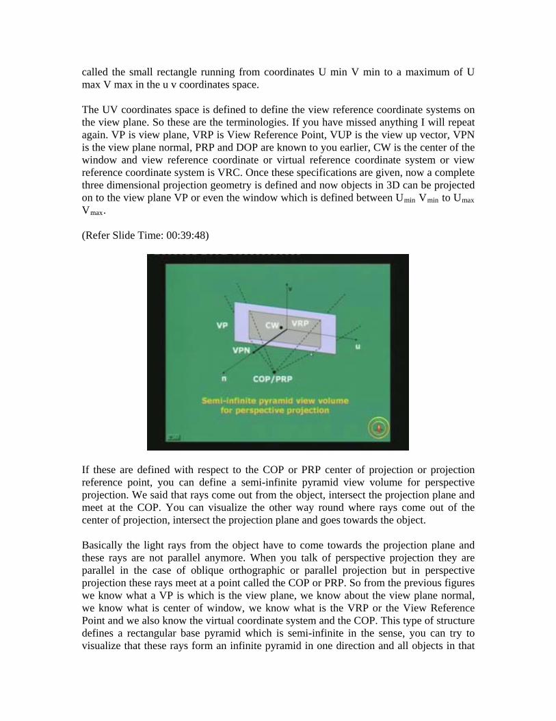
If these are defined with respect to the COP or PRP center of projection or projection reference point, you can define a semi-infinite pyramid view volume for perspective projection. We said that rays come out from the object, intersect the projection plane and meet at the COP. You can visualize the other way round where rays come out of the center of projection, intersect the projection plane and goes towards the object. Basically the light rays from the object have to come towards the projection plane and these rays are not parallel anymore. When you talk of perspective projection they are parallel in the case of oblique orthographic or parallel projection but in perspective projection these rays meet at a point called the COP or PRP. So from the previous figures we know what a VP is which is the view plane, we know about the view plane normal, we know what is center of window, we know what is the VRP or the View Reference Point and we also know the virtual coordinate system and the COP. This type of structure defines a rectangular base pyramid which is semi-infinite in the sense, you can try to visualize that these rays form an infinite pyramid in one direction and all objects in that

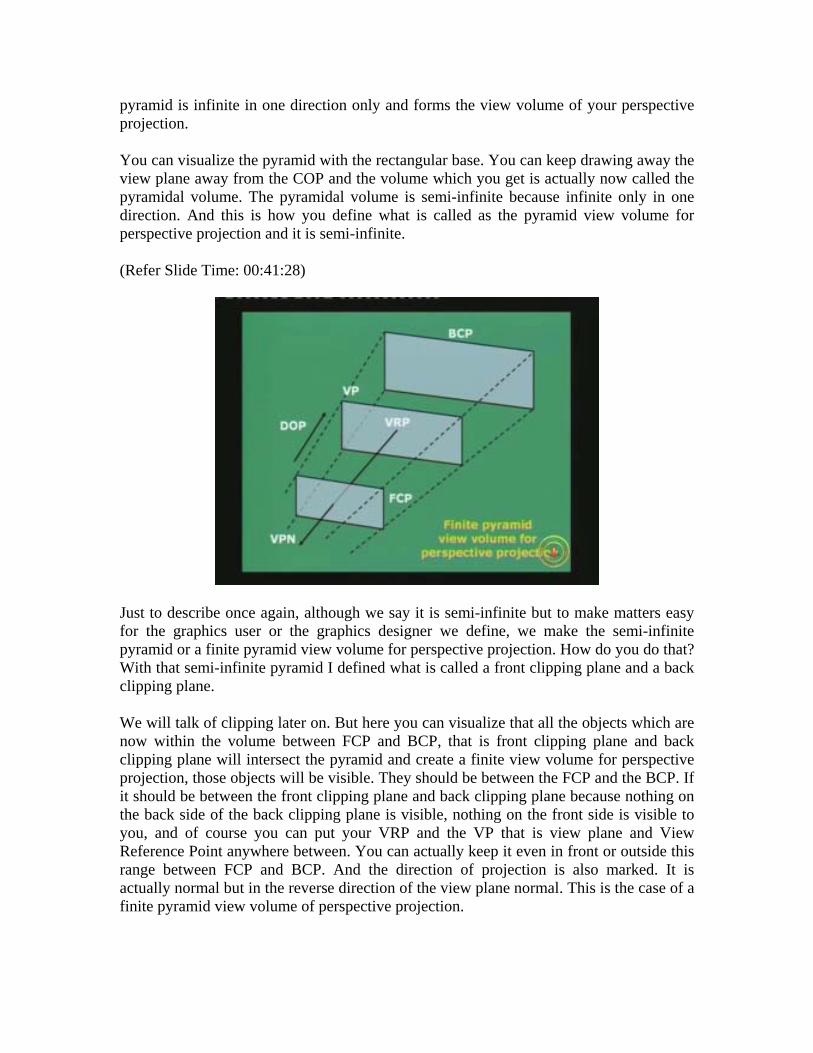
pyramid is infinite in one direction only and forms the view volume of your perspective projection. You can visualize the pyramid with the rectangular base. You can keep drawing away the view plane away from the COP and the volume which you get is actually now called the pyramidal volume. The pyramidal volume is semi-infinite because infinite only in one direction. And this is how you define what is called as the pyramid view volume for perspective projection and it is semi-infinite. (Refer Slide Time: 00:41:28)

Just to describe once again, although we say it is semi-infinite but to make matters easy for the graphics user or the graphics designer we define, we make the semi-infinite pyramid or a finite pyramid view volume for perspective projection. How do you do that? With that semi-infinite pyramid I defined what is called a front clipping plane and a back clipping plane. We will talk of clipping later on. But here you can visualize that all the objects which are now within the volume between FCP and BCP, that is front clipping plane and back clipping plane will intersect the pyramid and create a finite view volume for perspective projection, those objects will be visible. They should be between the FCP and the BCP. If it should be between the front clipping plane and back clipping plane because nothing on the back side of the back clipping plane is visible, nothing on the front side is visible to you, and of course you can put your VRP and the VP that is view plane and View Reference Point anywhere between. You can actually keep it even in front or outside this range between FCP and BCP. And the direction of projection is also marked. It is actually normal but in the reverse direction of the view plane normal. This is the case of a finite pyramid view volume of perspective projection.

I go back to the previous slide. This was the case of a semi-infinite pyramidal view volume and this is the case of a finite. So you can visualize yourself, both are pyramidal structures one is semi-infinite or almost infinite and this is a finite view volume. This finiteness comes from the two planes, the front clipping plane and the back clipping plane respectively. (Refer Slide Time: 0:43:05)

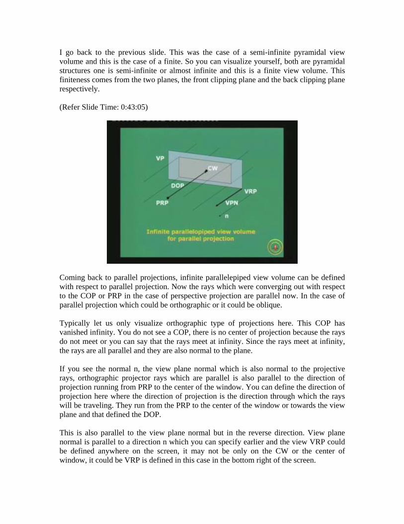
Coming back to parallel projections, infinite parallelepiped view volume can be defined with respect to parallel projection. Now the rays which were converging out with respect to the COP or PRP in the case of perspective projection are parallel now. In the case of parallel projection which could be orthographic or it could be oblique. Typically let us only visualize orthographic type of projections here. This COP has vanished infinity. You do not see a COP, there is no center of projection because the rays do not meet or you can say that the rays meet at infinity. Since the rays meet at infinity, the rays are all parallel and they are also normal to the plane. If you see the normal n, the view plane normal which is also normal to the projective rays, orthographic projector rays which are parallel is also parallel to the direction of projection running from PRP to the center of the window. You can define the direction of projection here where the direction of projection is the direction through which the rays will be traveling. They run from the PRP to the center of the window or towards the view plane and that defined the DOP. This is also parallel to the view plane normal but in the reverse direction. View plane normal is parallel to a direction n which you can specify earlier and the view VRP could be defined anywhere on the screen, it may not be only on the CW or the center of window, it could be VRP is defined in this case in the bottom right of the screen.

You are free to define this coordinates but where, of course certain constraints and it should be all consistent with respect to each other. The VRP could be anywhere in the view plane center of window is the center of the view port, the grey color center window and PRP, the line joining PRP the center of window is the direction of projection. That is the infinite parallelepiped view volume, why infinite? It is infinite because if you see I have drawn four such rays which are intersecting the projection plane normally and they move on both directions towards infinity. And you can visualize that I have got a rectangular parallelepiped of infinite size. So the depth basically, there is a height and or the length and the breath but along the Z axis or along the direction of projection it is infinite. So that is an infinite view volume like an infinite pyramid which we had in the case of perspective but now this infinite pyramid becomes an infinite parallelepiped in the case of parallel projection just to define it more in a better form. (Refer Slide Time: 00:45:34)

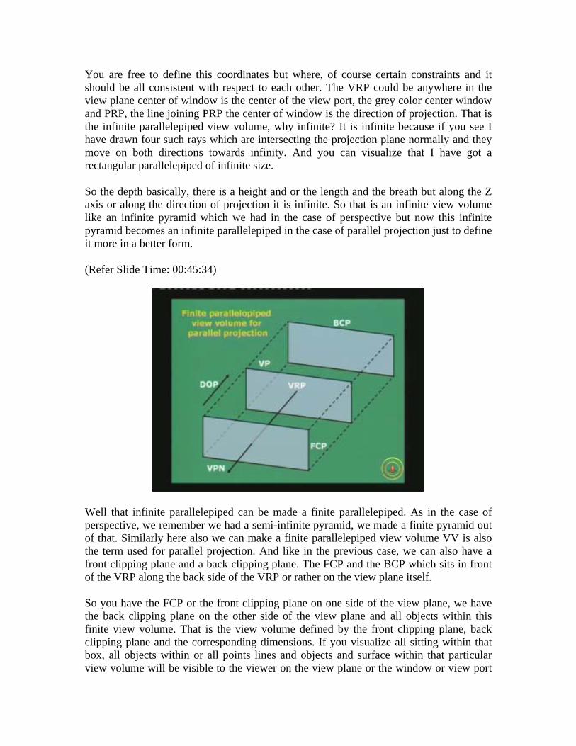
Well that infinite parallelepiped can be made a finite parallelepiped. As in the case of perspective, we remember we had a semi-infinite pyramid, we made a finite pyramid out of that. Similarly here also we can make a finite parallelepiped view volume VV is also the term used for parallel projection. And like in the previous case, we can also have a front clipping plane and a back clipping plane. The FCP and the BCP which sits in front of the VRP along the back side of the VRP or rather on the view plane itself. So you have the FCP or the front clipping plane on one side of the view plane, we have the back clipping plane on the other side of the view plane and all objects within this finite view volume. That is the view volume defined by the front clipping plane, back clipping plane and the corresponding dimensions. If you visualize all sitting within that box, all objects within or all points lines and objects and surface within that particular view volume will be visible to the viewer on the view plane or the window or view port

which you define and all objects which are outside this view volume will not be visible. It is always good to define a finite view volume either in the case of parallel or perspective so that you know what are the range or the dimensions, range of values along each XY XY and Z directions which are visible to you. Of course if you take a digital camera or if you are seeing through your own eye you know that only a finite range of the world is visible to you and that too in front and a little bit to this side and top and down. You may definitely not be able to see what is on the back side of you, you may not be able to see the objects which are too far from you on the front side and also definitely on both sides if they are highly oblique to the left and right side and you will not be able to see the object in the two extremes. So you will always see, of course in the digital camera and in our eye we have a perspective nature of viewing but either perspective or parallel, you always see a finite region in space or in the world whatever. And henceforth you always have a back clipping plane and a front clipping plane and of course the two dimensions on two sides, you will not be able to definitely see what is at the back of you on the viewers. With respect to these points I would like to wind up the discussions on three dimensional transformations and move on to the next lecture which will basically be an extension of three dimensional transformations. But I have given it in to different name which will be going towards three dimensional viewing and clipping. Although there is a separate chapter on clipping algorithms but three dimensional viewing geometry and all that I thought to keep it separate from three dimensional transformations. We will discuss that in the next one or two classes as we go along. But before that I have given here a list of problems and exercises which you should try to solve based on the last two to three hours of lecturing which we have done so far. As we go along of course I was also stating problems to you which you should workout all these mathematics which is given to you, you should draw those diagrams yourself, you should try to derive those equations, expressions for the generalized transformations of all the matrices in terms of especially rotation, reflection and perspective transformation matrices. You should derive all those expressions yourself at least once or twice and then only you will get the confidence. And in addition to this I must also mention here that I have given a few more problems which you can workout. I will just read out these problems. The first problem says illustrate the vanishing points for the projection of a transparent cube in case of the three point perspective projection. Remember, as we went through these lectures we talked about one point, two points and three point perspective geometric or projection models. But I have only given figures for one point projection and two point projection systems. So you will be able to visualize now, what will be scenario of the projection plane such that you obtain in the case of a cube, a three point perspective projection. Visualize this and then try to draw and take a sheet of paper and try to draw projective rays, get the intersection points on the projection planes and then try to obtain the three vanishing points in the case of a cube for a three point projection.

Question number 2 says, obtain the expression of the elements of the matrices which provide the generalized transformations in case of rotation about an arbitrary axis and reflection about an arbitrary plane. Now I have given the expression in matrix multiplication form and I have worked out the expressions of the elements of each of these matrices may be two classes back. Remember, we had a composite form which composed of translations, rotations and reflection also. In question two b, but I have not taken those two expressions and multiplied all those matrices and obtained the fundamental form. Please do that, it will give a lot of confidence both in terms of matrix algebra and also in terms of matrix manipulation with the elements and also confidence with respect to these aspects of three dimensional transformations here in computer graphics. So take those expressions which are given there separately. Take the composite form, substitute them one by one or sequentially keep multiplying and obtain all the 9 or 16 elements. It is a 3/3 or a 4/4, you could do this in 2D as well. With this in 2D of course, rotation is about a point and reflection is about a line. In the case of 3D we remember the rotation is respect to an arbitrary axis, generalized transformation I am talking about and reflection will be with respect to a plane. So plane on an axis is 3D becomes a point and line in 2D. If you find the 3D transformation matrix to be you can go back to 2D, take the generalized transformation matrices in 2D and try to get the expression of the matrix. I have given the separate forms please multiply them. A special case of question two is question three where I am asking you to obtain a matrix which is a multiplication of that obtaining 2a and 2b. So whatever answer you get in two a two b, you multiply them and get another matrix. What will this matrix give you? This matrix will actually give you a form of two successive operations of rotation and reflection, a generalized one. That means if you want to rotate about an arbitrary axis and then reflect about an arbitrary plane or even the vice versa. If it is reversed, the transformations of 2a into 2b or 2b then 2a, whatever the case may be, the answer which you get in question three will give you the generalized transformation matrix which involves a composite matrix of two generalized transformations. What are those two generalized transformations in sequence? Rotation about an axis and reflection about a plane or in 2D it is rotation about a point and reflection about a line so that is question number three. Question number four is a very interesting observation. Take the rotation matrix in 2D or three D and prove that pure rotation about an arbitrary axis in 3D or a point in case of 2D can be considered as a combination of another rotation and a translation. I leave this as an exercise for you to try out. That means if you rotate by an amount theta what you basically do is take another matrix where you rotate by an amount if it is a fraction of theta or theta by two let us say. And to reach to the final point which you

would have rotated by theta you need a translation which you can do because you are talking of a point. We are talking with respect to a point, so a combination of a rotation and a translation gives you another rotation about a point or any arbitrary rotation can be expressed as a rotation and then a translation to the final destination point. So you can prove that very easily. You can do it in 3D or 2D by taking the rotational matrices. Basically what you have to do is, find the expressions of that translation components required to take you to that final point which you would have reached by a pure rotation. The last question is, obtain the scale matrix along an arbitrary direction. It is interesting here because the scale matrix which you have thought of is a generalized scale matrix which will scale in all directions or we have scale coefficients along x y and z. Now I say scale along a vector 1 1 1 or any arbitrary vector which gives you the direction cosines along a particular direction. And I will ask you to scale along that particular direction. That means I am asking you to derive in the last question, a generalized expression or a generalized transformation matrix for scaling like we did for rotation, reflection, perspective transformation and now do it for scaling because we have got the scaling matrices for special cases along x y or z or all together. So given along a particular arbitrary direction what should be the scale matrix. Please try to solve all these problems as given here and also the problems which I have talked of earlier. It will give you a lot of confidence both in terms of vector algebra, matrix algebra and transformation matrix in both 2D and 3D transformations. So we stop here and move towards the next lecture which will be on three dimensional transformation and leave. Thank you very much.

Documents

Computer Graphics Prof. Sukhendu Das Dept. of …textofvideo.nptel.ac.in/106106090/lec10.pdfSo we are basically projecting on to a two dimensional plane which is the screen and this