Computer Graphics I

- Image based Rendering -

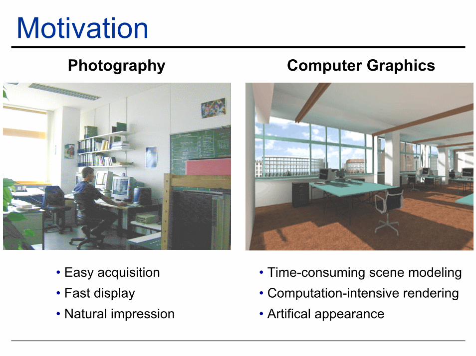
MotivationComputer GraphicsPhotography

• Easy acquisition• Fast display • Natural impression

• Time-consuming scene modeling• Computation-intensive rendering • Artifical appearance

Motivation II

• All we usually care about in rendering is generating images from new viewpoints

Motivation II

• All we usually care about in rendering is generating images from new viewpoints

• In geometry-based methods, we compute these new images– Projection– Lighting– Z-buffering

Motivation II

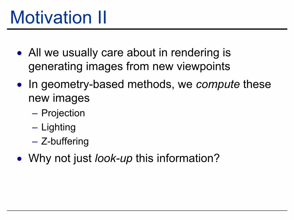
• All we usually care about in rendering is generating images from new viewpoints

• In geometry-based methods, we compute these new images– Projection– Lighting– Z-buffering

• Why not just look-up this information?

Overview

• Theoretical Basis• “Pure” IBR Algorithms• Geometry-assisted IBR Techniques

Overview• Plenoptic function• Panoramas• Concentric Mosaics• Light Field Rendering• The Lumigraph• Layered Depth Images• View-dependent Texture Mapping• Surface Light Fields• View Morphing

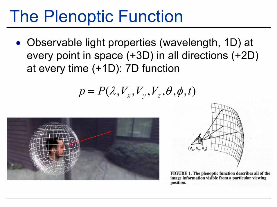
The Plenoptic Function• Observable light properties (wavelength, 1D) at

every point in space (+3D) in all directions (+2D) at every time (+1D): 7D function

),,,,,,( tVVVPp zyx φθλ=

The Plenoptic Function II• Acquisition

– Continuous function ⇒ appropriate discretization– High-dimensional ⇒ reduction in storage

requirements

• Rendering– Continuous function ⇒ look up function value– Discretized data ⇒ re-sample and interpolate

Plenoptic Rendering Taxonomy• Reduced Plenoptic Function

– 5D: time and wavelength omitted ⇒ static scene, RGB values

• Light Field Rendering– 4D: transparent space, viewpoint outside bounding

box

• Concentric Mosaics– 3D: viewpoint constrained to lie within a circle

• Panoramas– 2D: fixed viewpoint

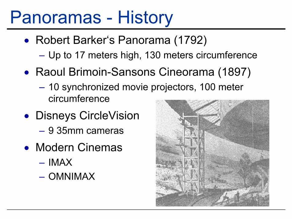
Panoramas - History• Robert Barker‘s Panorama (1792)

– Up to 17 meters high, 130 meters circumference

• Raoul Brimoin-Sansons Cineorama (1897)– 10 synchronized movie projectors, 100 meter

circumference

• Disneys CircleVision– 9 35mm cameras

• Modern Cinemas– IMAX– OMNIMAX

PanoramasFixed viewpoint, arbitrary viewing direction• Acquisition

− multiple conventional images− Special panorama cameras

• Mosaicing− Image registration− Stitching− Warping

• Rendering− Resampling in real-time

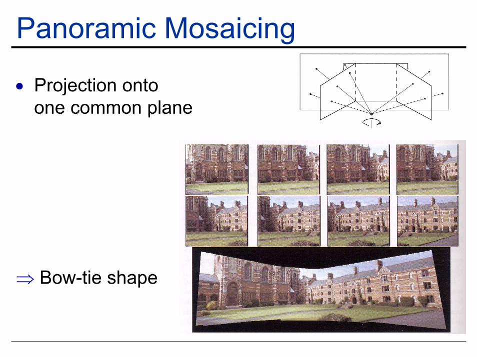
Panoramic Mosaicing

• Projection onto one common plane

⇒ Bow-tie shape

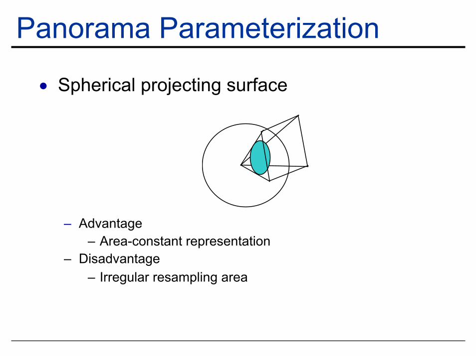
Panorama Parameterization

• Spherical projecting surface

– Advantage– Area-constant representation

– Disadvantage– Irregular resampling area

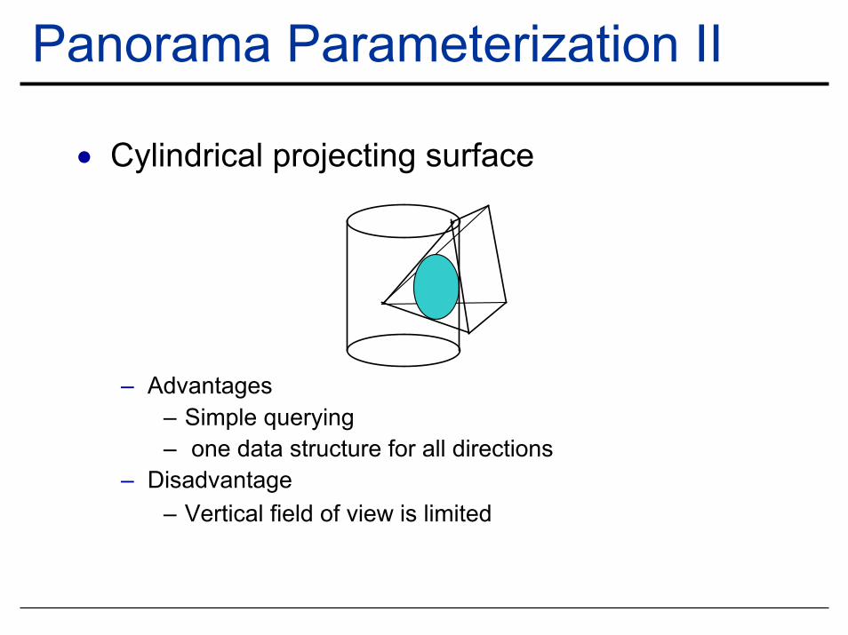
Panorama Parameterization II

• Cylindrical projecting surface

– Advantages– Simple querying– one data structure for all directions

– Disadvantage– Vertical field of view is limited

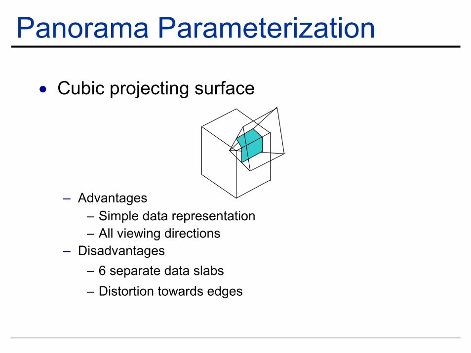
Panorama Parameterization

• Cubic projecting surface

– Advantages– Simple data representation– All viewing directions

– Disadvantages– 6 separate data slabs– Distortion towards edges

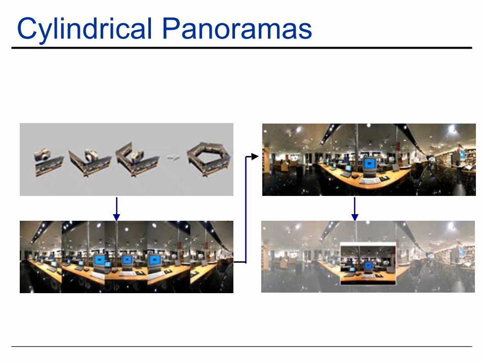
Cylindrical Panoramas

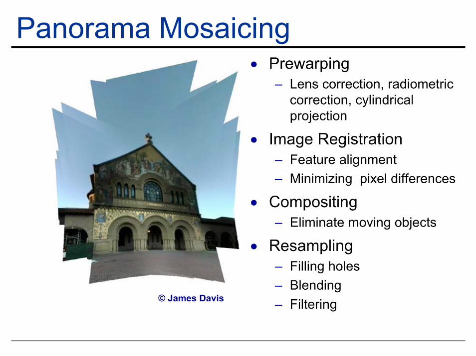
Panorama Mosaicing• Prewarping

– Lens correction, radiometric correction, cylindrical projection

• Image Registration– Feature alignment– Minimizing pixel differences

• Compositing– Eliminate moving objects

• Resampling– Filling holes– Blending– Filtering© James Davis

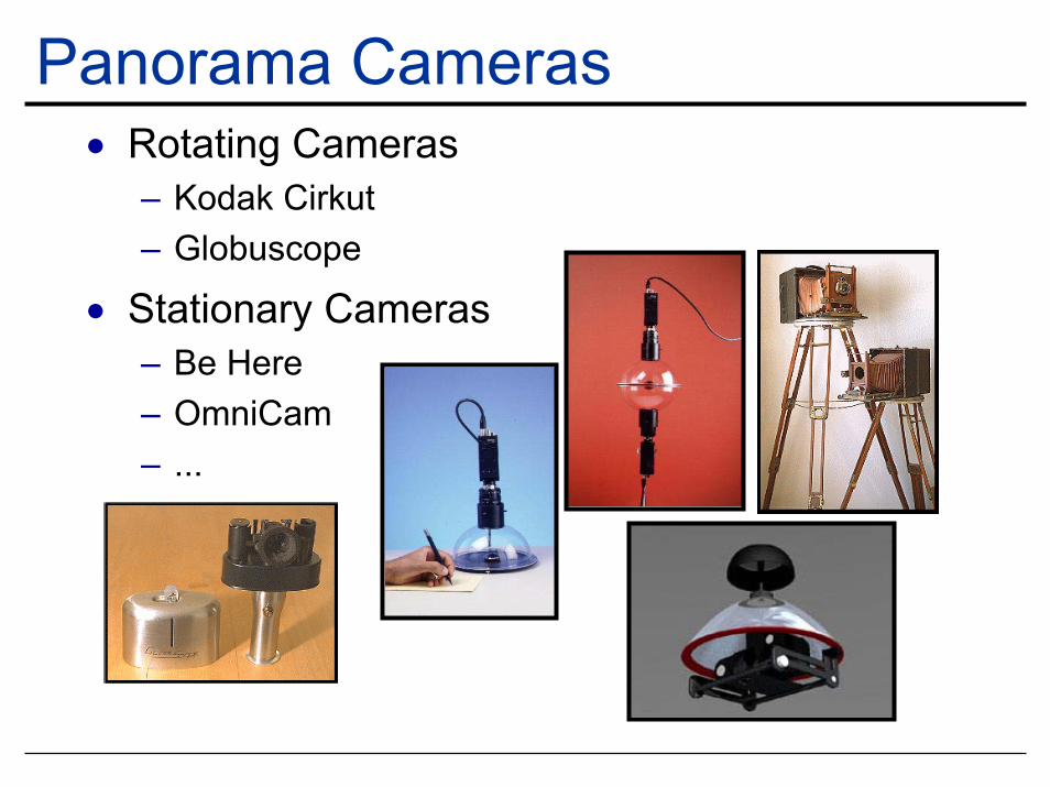
Panorama Cameras• Rotating Cameras

– Kodak Cirkut– Globuscope

• Stationary Cameras– Be Here– OmniCam– ...

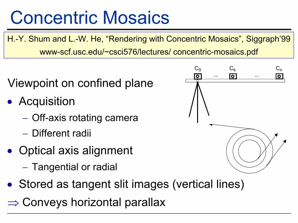
Concentric MosaicsH.-Y. Shum and L.-W. He, “Rendering with Concentric Mosaics”, Siggraph’99

www-scf.usc.edu/~csci576/lectures/ concentric-mosaics.pdf

Viewpoint on confined plane• Acquisition

− Off-axis rotating camera− Different radii

• Optical axis alignment− Tangential or radial

• Stored as tangent slit images (vertical lines) ⇒ Conveys horizontal parallax

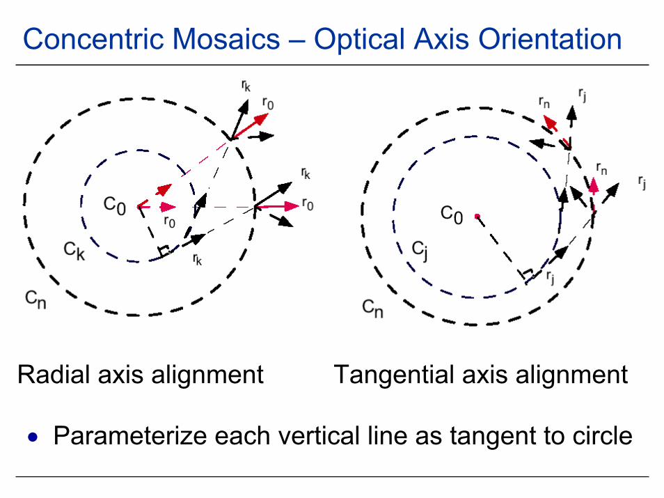
Concentric Mosaics – Optical Axis Orientation

Radial axis alignment Tangential axis alignment

• Parameterize each vertical line as tangent to circle

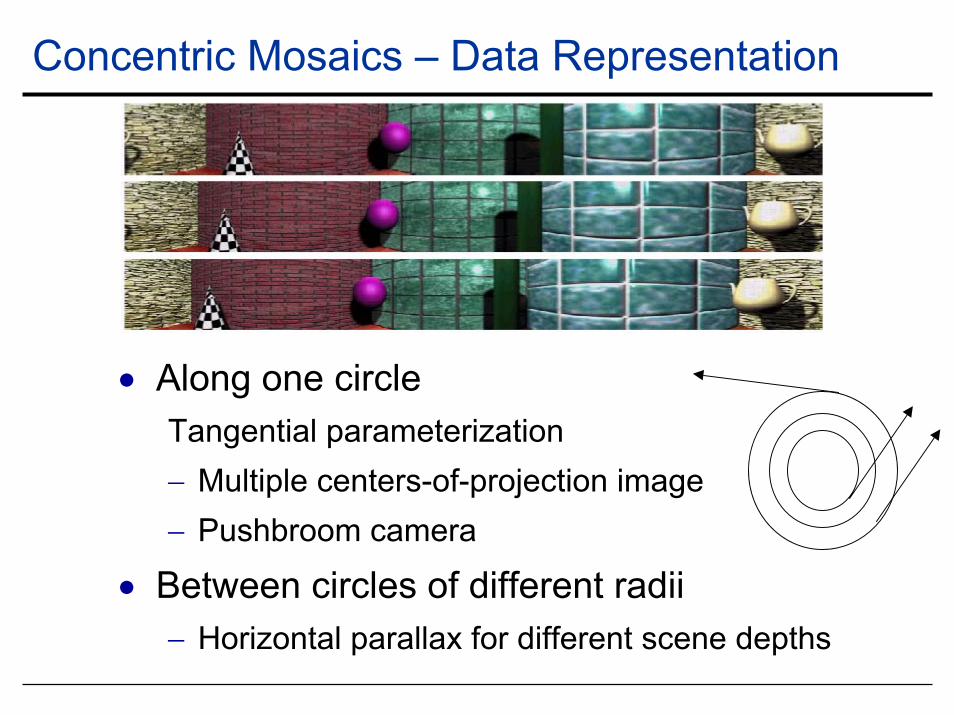
Concentric Mosaics – Data Representation

• Along one circleTangential parameterization− Multiple centers-of-projection image− Pushbroom camera

• Between circles of different radii− Horizontal parallax for different scene depths

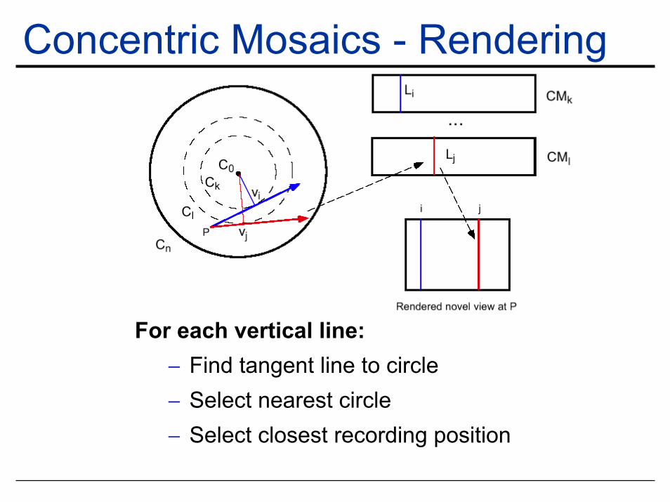
Concentric Mosaics - Rendering

For each vertical line:− Find tangent line to circle− Select nearest circle − Select closest recording position

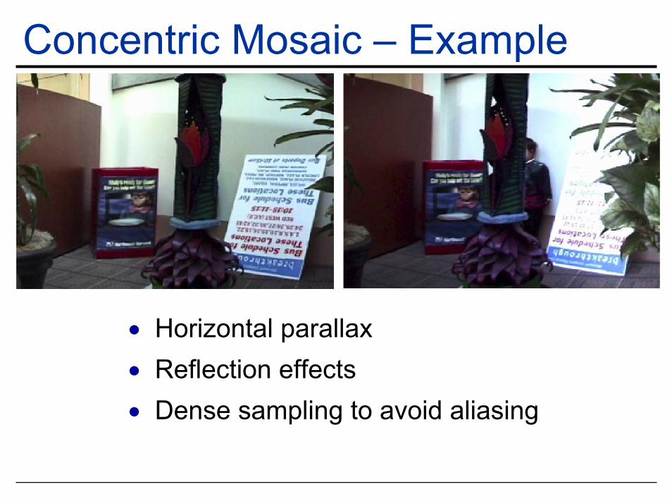
Concentric Mosaic – Example

• Horizontal parallax• Reflection effects• Dense sampling to avoid aliasing

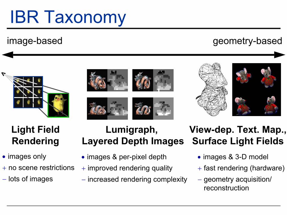
IBR Taxonomyimage-based geometry-based

Lumigraph, Layered Depth Images• images & per-pixel depth+ improved rendering quality− increased rendering complexity

View-dep. Text. Map.,Surface Light Fields

• images & 3-D model+ fast rendering (hardware)− geometry acquisition/

reconstruction

Light FieldRendering

• images only+ no scene restrictions− lots of images

Light Field RenderingLevoy and Hanrahan, “Light Field Rendering”, Siggraph’96

graphics.stanford.edu/projects/lightfield/

• Viewpoint outside bounding visual hull• Assumption: light properties don’t change along ray• 2D matrix of 2D images: 4D structure⇒ Conveys full parallax⇒ captures complex BRDFs

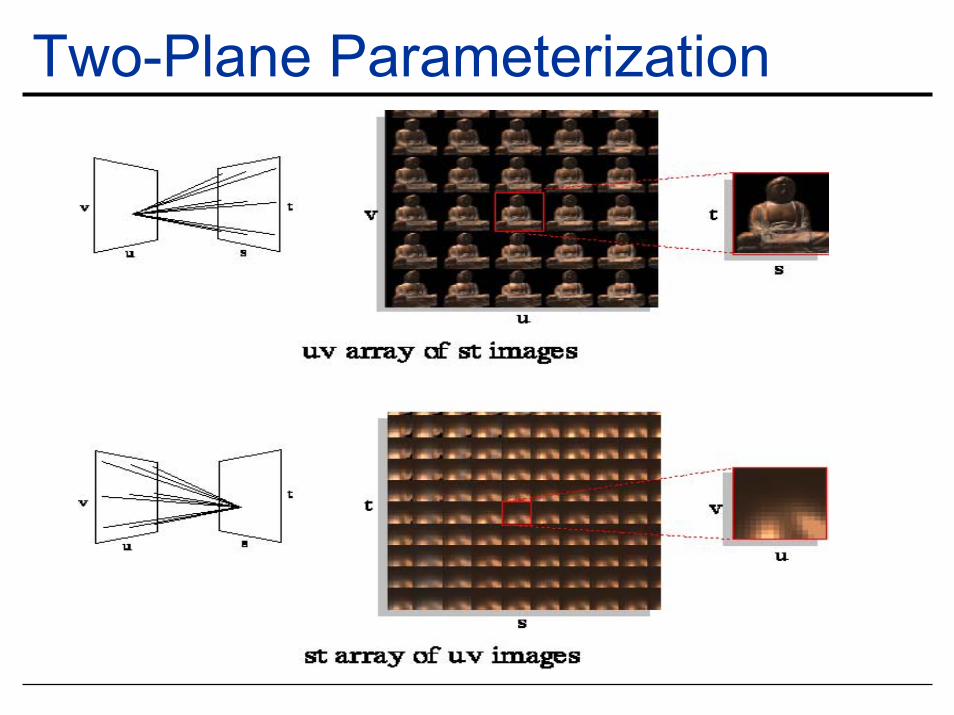
Two-Plane Parameterization

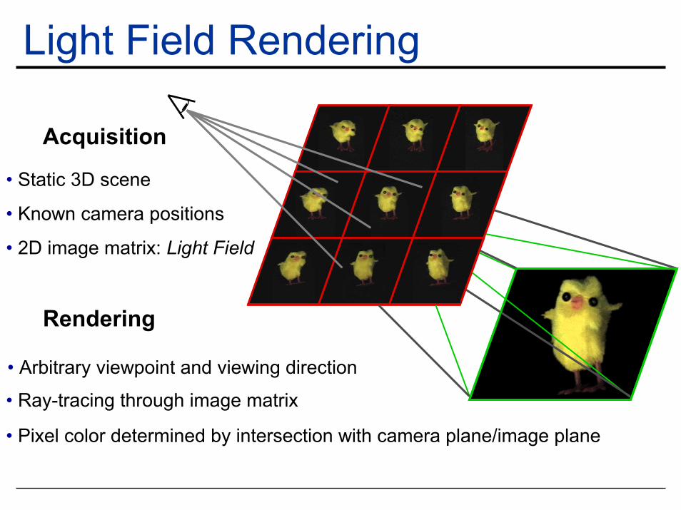
Light Field Rendering

• Known camera positions

• 2D image matrix: Light Field

• Arbitrary viewpoint and viewing direction

• Ray-tracing through image matrix

• Static 3D scene

Acquisition

Rendering

• Pixel color determined by intersection with camera plane/image plane

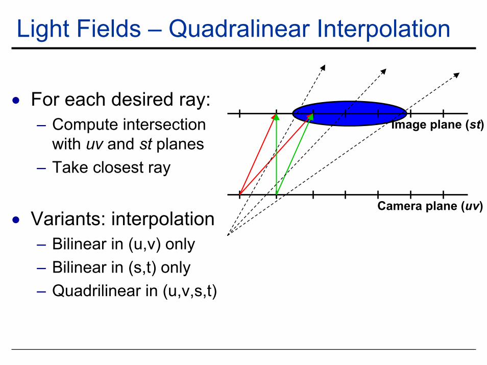
Light Fields – Quadralinear Interpolation

Image plane (st)

Camera plane (uv)

• For each desired ray:– Compute intersection

with uv and st planes– Take closest ray

• Variants: interpolation– Bilinear in (u,v) only– Bilinear in (s,t) only– Quadrilinear in (u,v,s,t)

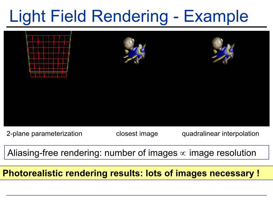
Light Field Rendering - Example

2-plane parameterization closest image quadralinear interpolation

Aliasing-free rendering: number of images ∝ image resolution

Photorealistic rendering results: lots of images necessary !

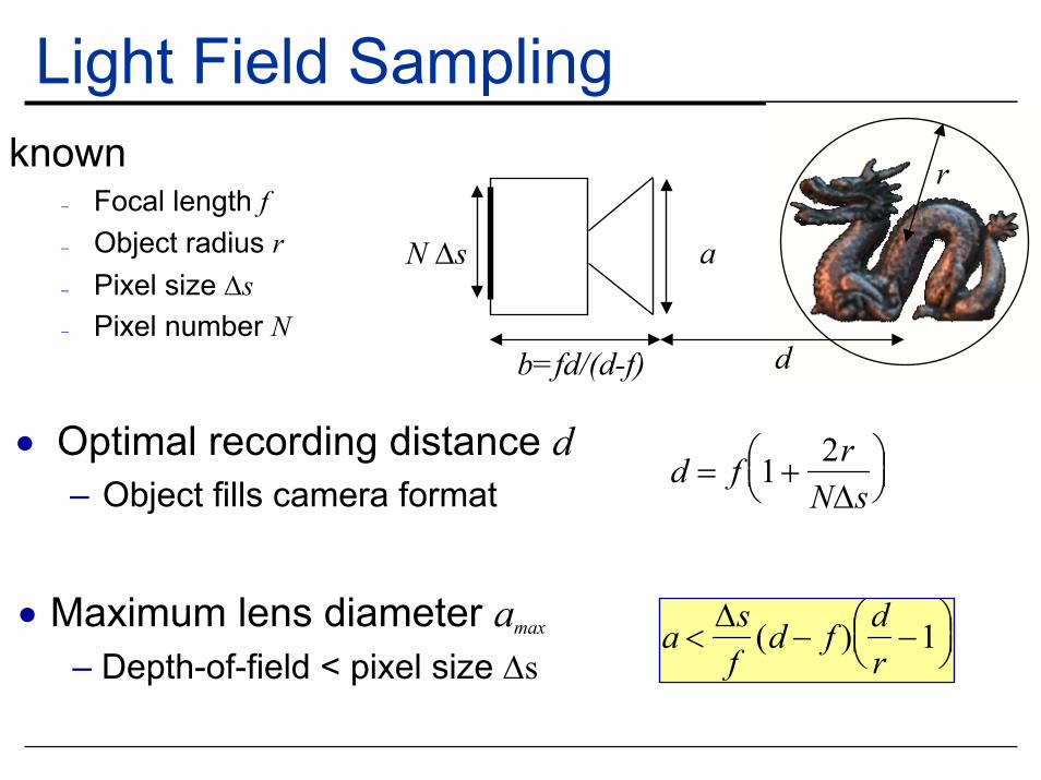
Light Field Sampling

d

r

b=fd/(d-f)

N ∆s a

known− Focal length f− Object radius r− Pixel size ∆s− Pixel number N

d

• Optimal recording distance d– Object fills camera format

d = f 1 +2r

N∆s

a <∆sf

(d − f ) dr

−1

• Maximum lens diameter amax

– Depth-of-field < pixel size ∆s

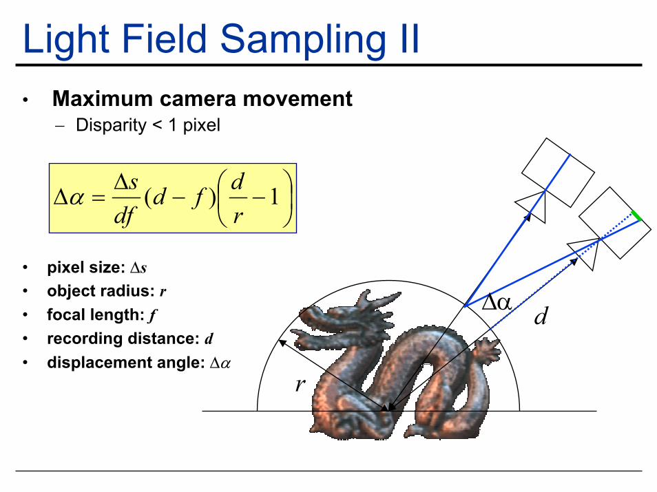
Light Field Sampling II• Maximum camera movement

− Disparity < 1 pixel

−−

∆=∆ 1)(

rdfd

dfsα

d

r

∆α• pixel size: ∆s• object radius: r• focal length: f• recording distance: d• displacement angle: ∆α

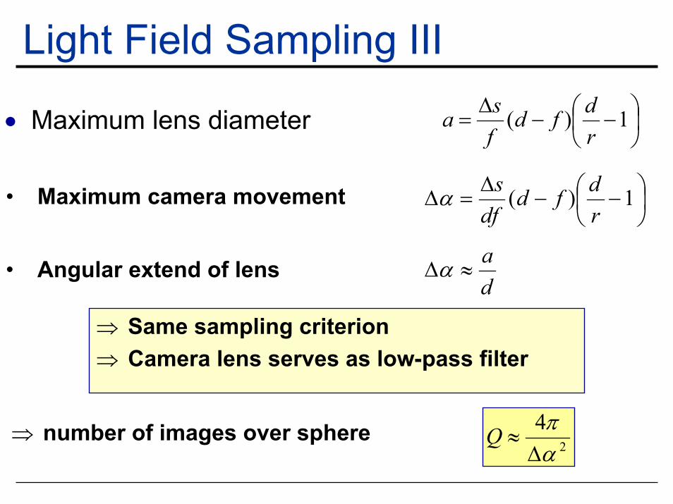
Light Field Sampling III

• Maximum lens diameter

−−

∆= 1)(

rdfd

fsa

−−

∆=∆ 1)(

rdfd

dfsα• Maximum camera movement

da

≈∆α• Angular extend of lens

⇒ Same sampling criterion⇒ Camera lens serves as low-pass filter

2

4απ

∆≈Q⇒ number of images over sphere

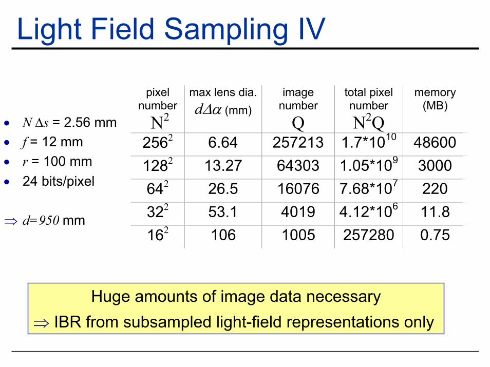
Light Field Sampling IV

pixel number N2

max lens dia.d∆α (mm)

image number

Q

total pixel number N2Q

memory (MB)

2562 6.64 257213 1.7*1010 486001282 13.27 64303 1.05*109 3000 642 26.5 16076 7.68*107 220 322 53.1 4019 4.12*106 11.8 162 106 1005 257280 0.75

• N ∆s = 2.56 mm• f = 12 mm• r = 100 mm• 24 bits/pixel

⇒ d=950 mm

Huge amounts of image data necessary⇒ IBR from subsampled light-field representations only

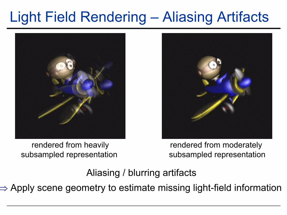
Light Field Rendering – Aliasing Artifacts

rendered from heavilysubsampled representation

rendered from moderately subsampled representation

Aliasing / blurring artifacts⇒ Apply scene geometry to estimate missing light-field information

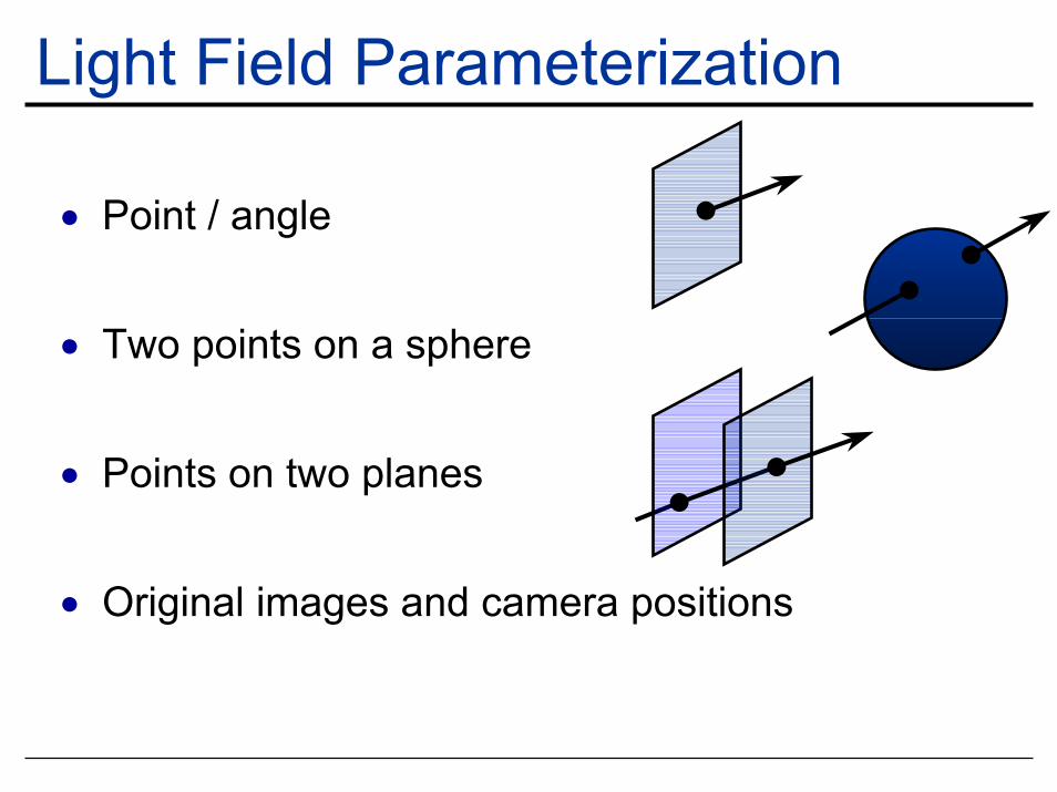
Light Field Parameterization

• Point / angle

• Two points on a sphere

• Points on two planes

• Original images and camera positions

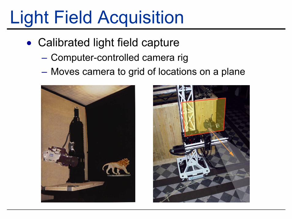
Light Field Acquisition• Calibrated light field capture

– Computer-controlled camera rig– Moves camera to grid of locations on a plane

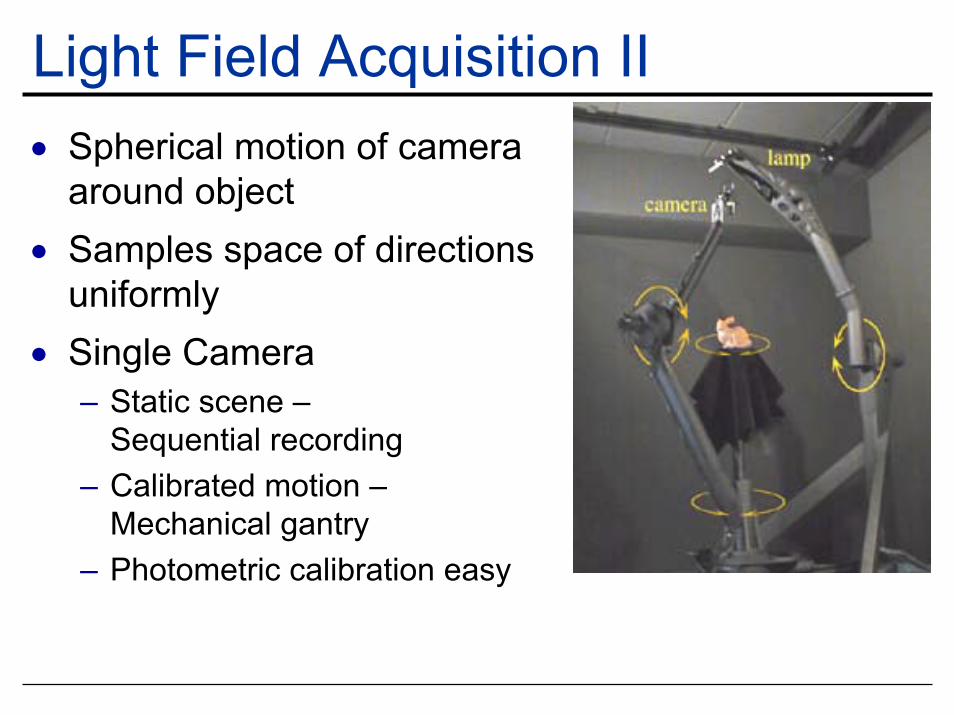
Light Field Acquisition II• Spherical motion of camera

around object• Samples space of directions

uniformly• Single Camera

– Static scene –Sequential recording

– Calibrated motion –Mechanical gantry

– Photometric calibration easy

Light Fields - Summary• Advantages

– Simpler computation vs. traditional CG– Cost independent of scene complexity– Cost independent of material properties

and other optical effects

• Disadvantages– Static geometry– Fixed lighting– High storage cost / aliasing

Geometry-assisted IBR Methods

• Fundamental idea of IBR:Generate new views of a scene directly from recorded views

• “Pure” IBR ⇒ Light Field Rendering• Enormous amount of images necessary• Highly redundant data• Other IBR techniques try to obtain higher

quality with less storage by exploiting scene geometry information

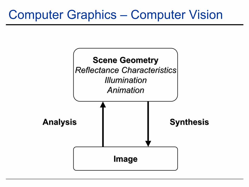
Computer Graphics – Computer Vision

ImageImage

AnalysisAnalysis SynthesisSynthesis

Scene GeometryScene GeometryReflectance CharacteristicsReflectance Characteristics

IlluminationIlluminationAnimationAnimation

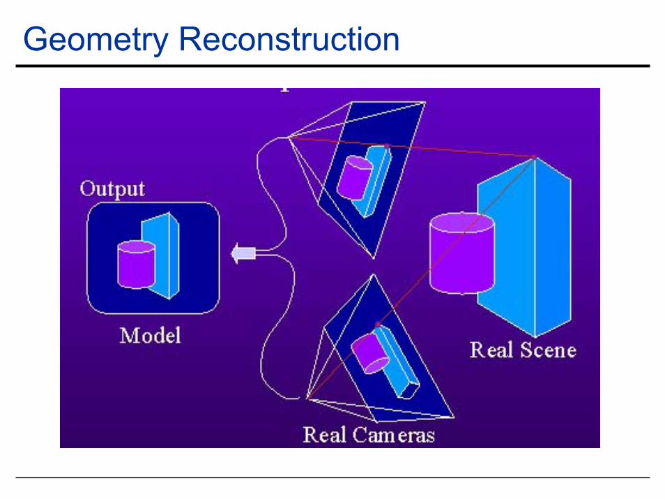
Geometry Reconstruction

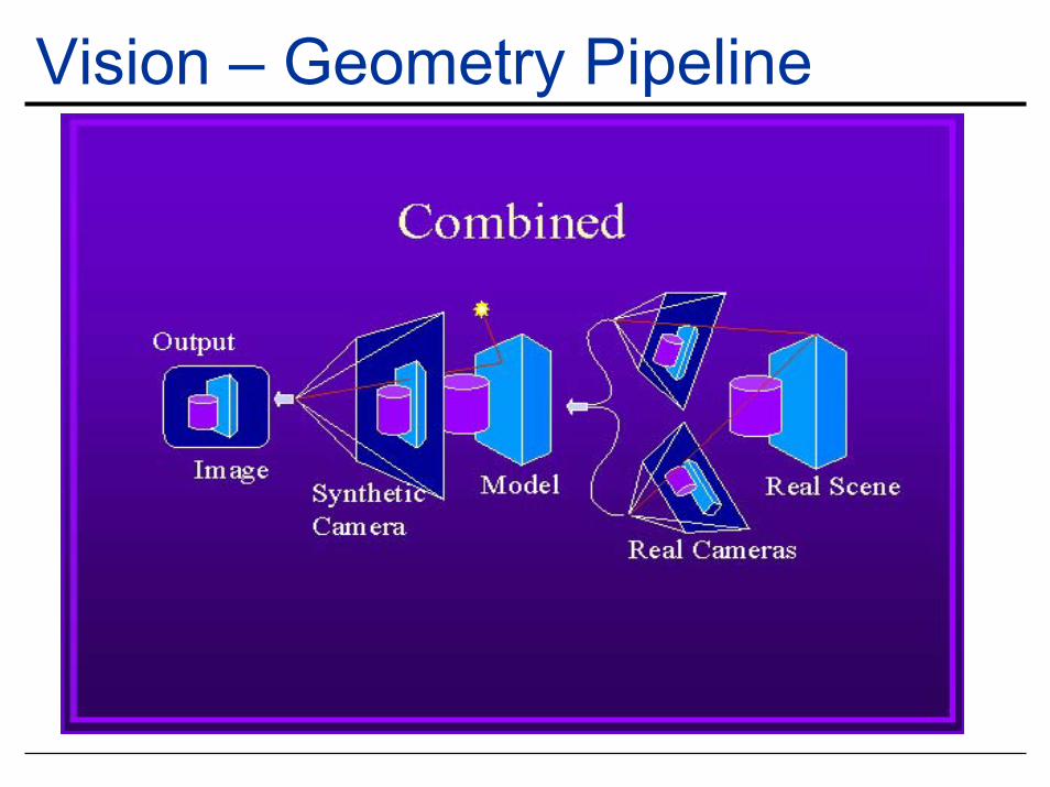
Vision – Geometry Pipeline

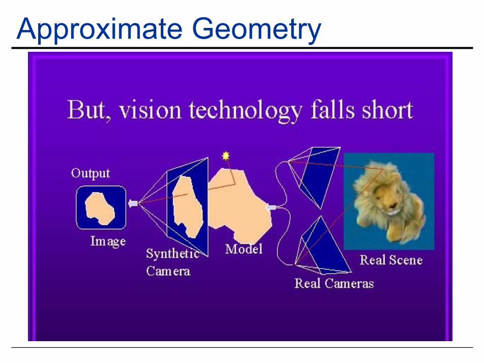
Approximate Geometry

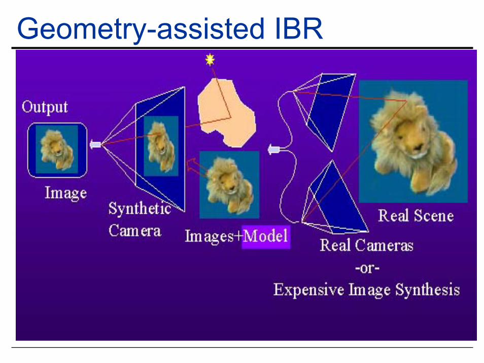
Geometry-assisted IBR

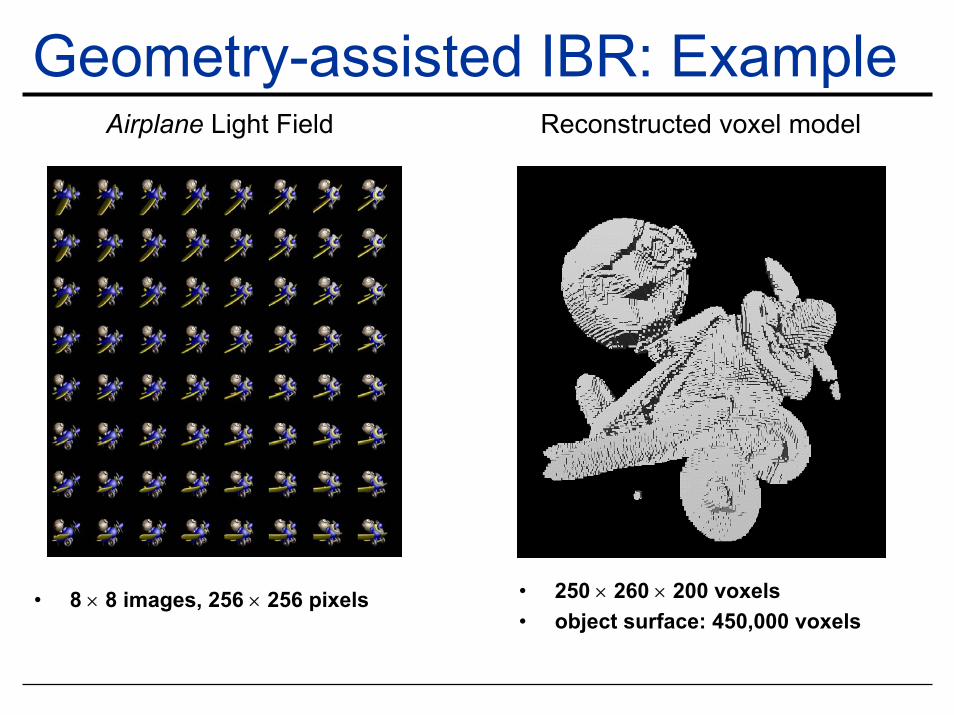
Geometry-assisted IBR: ExampleAirplane Light Field Reconstructed voxel model

• 250 × 260 × 200 voxels• object surface: 450,000 voxels

• 8 × 8 images, 256 × 256 pixels

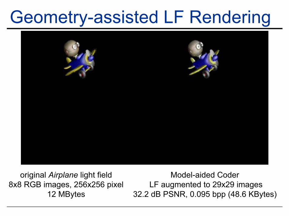
Geometry-assisted LF Rendering

original Airplane light field8x8 RGB images, 256x256 pixel

12 MBytes

Model-aided CoderLF augmented to 29x29 images

32.2 dB PSNR, 0.095 bpp (48.6 KBytes)

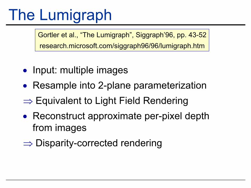
The LumigraphGortler et al., “The Lumigraph”, Siggraph’96, pp. 43-52research.microsoft.com/siggraph96/96/lumigraph.htm

• Input: multiple images• Resample into 2-plane parameterization⇒ Equivalent to Light Field Rendering• Reconstruct approximate per-pixel depth

from images⇒ Disparity-corrected rendering

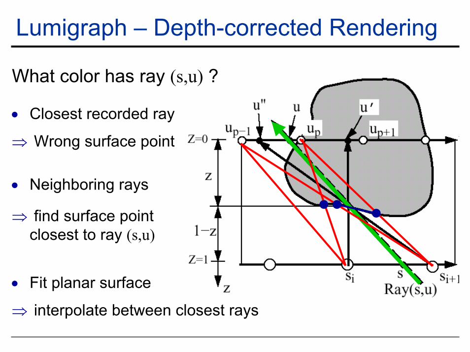
Lumigraph – Depth-corrected Rendering

• Closest recorded ray

• Neighboring rays

⇒ find surface pointclosest to ray (s,u)

⇒ interpolate between closest rays

⇒ Wrong surface point

What color has ray (s,u) ?

• Fit planar surface

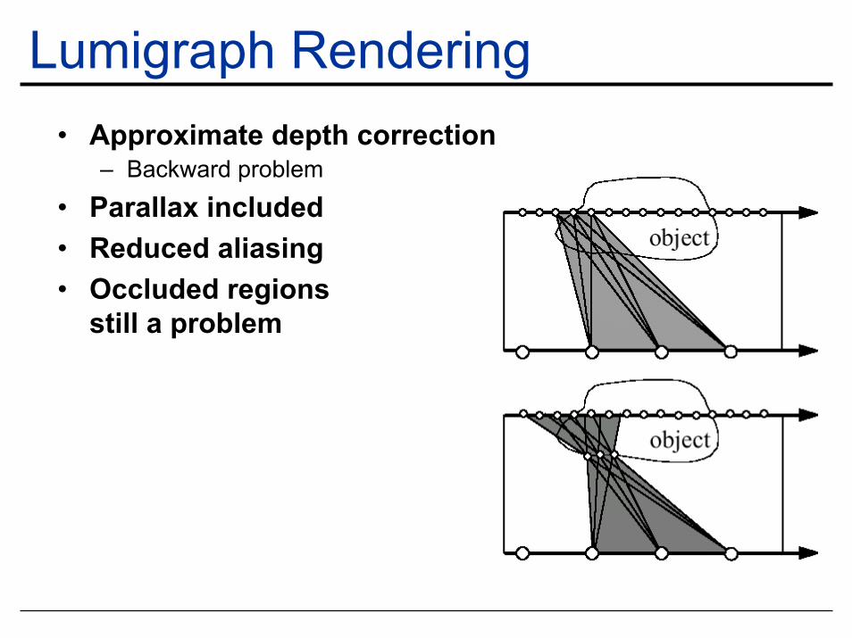
Lumigraph Rendering• Approximate depth correction

– Backward problem• Parallax included• Reduced aliasing• Occluded regions

still a problem

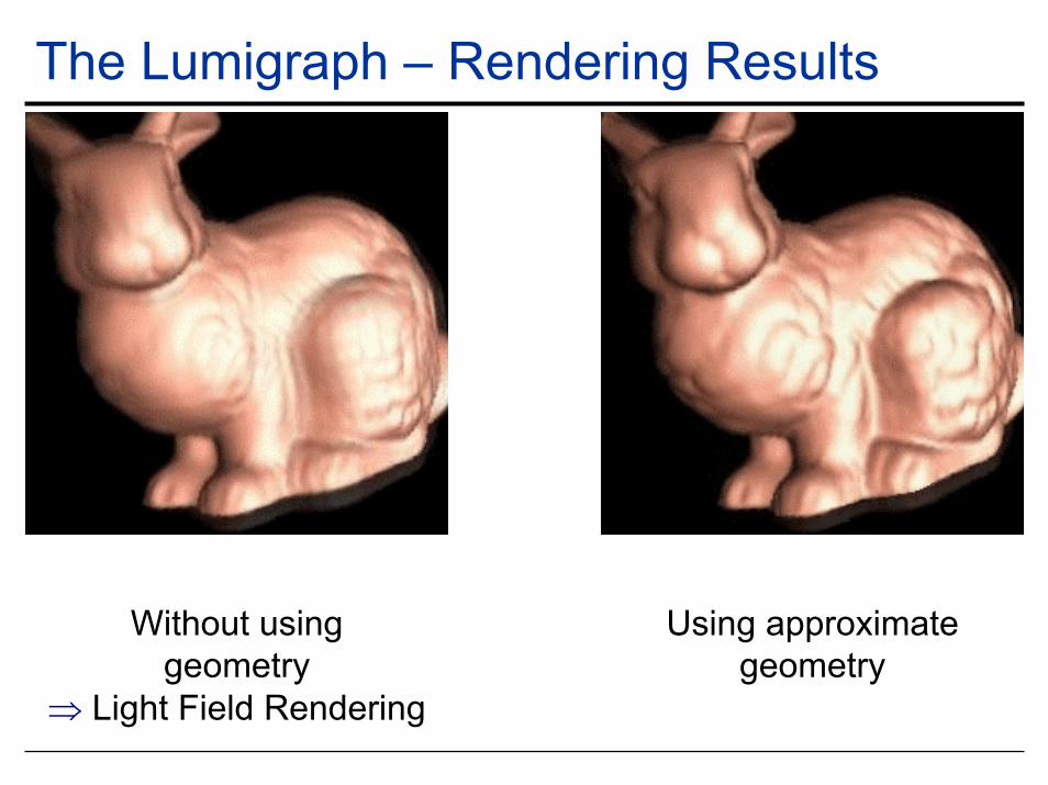
The Lumigraph – Rendering Results

Without usinggeometry

⇒ Light Field Rendering

Using approximategeometry

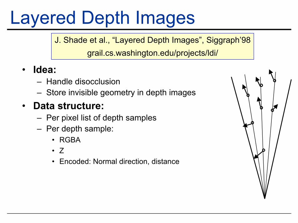
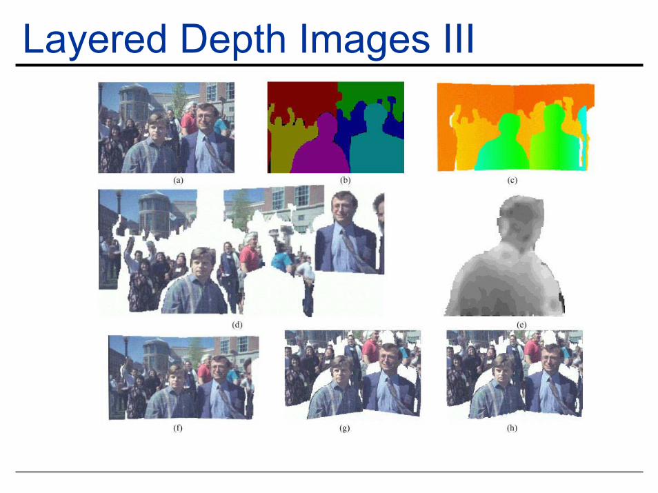
Layered Depth ImagesJ. Shade et al., “Layered Depth Images”, Siggraph’98

grail.cs.washington.edu/projects/ldi/

• Idea:– Handle disocclusion– Store invisible geometry in depth images

• Data structure:– Per pixel list of depth samples– Per depth sample:

• RGBA• Z• Encoded: Normal direction, distance

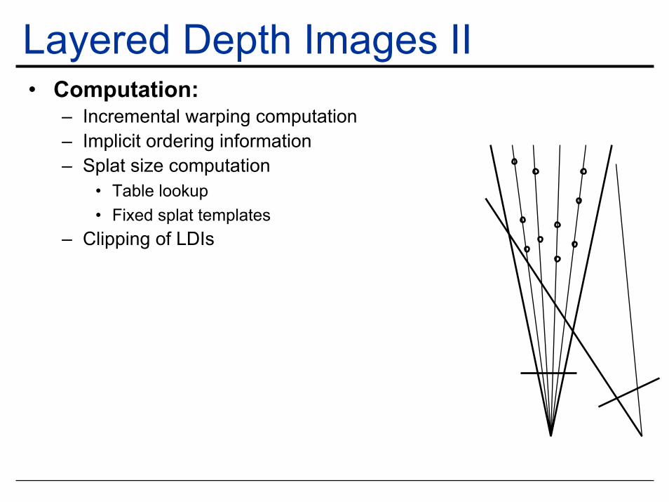
Layered Depth Images II• Computation:

– Incremental warping computation– Implicit ordering information– Splat size computation

• Table lookup• Fixed splat templates

– Clipping of LDIs

Layered Depth Images III

View MorphingS. Seitz and C. Dyer, “View Morphing”, Siggraph’96

www.cs.washington.edu/homes/seitz/vmorph/vmorph.htm

• Warping between 2 (or more) images• Cameras’ F matrices known • Image correspondences known for all pixels⇒ Continuously warp one image into the other

giving a physically plausible impression

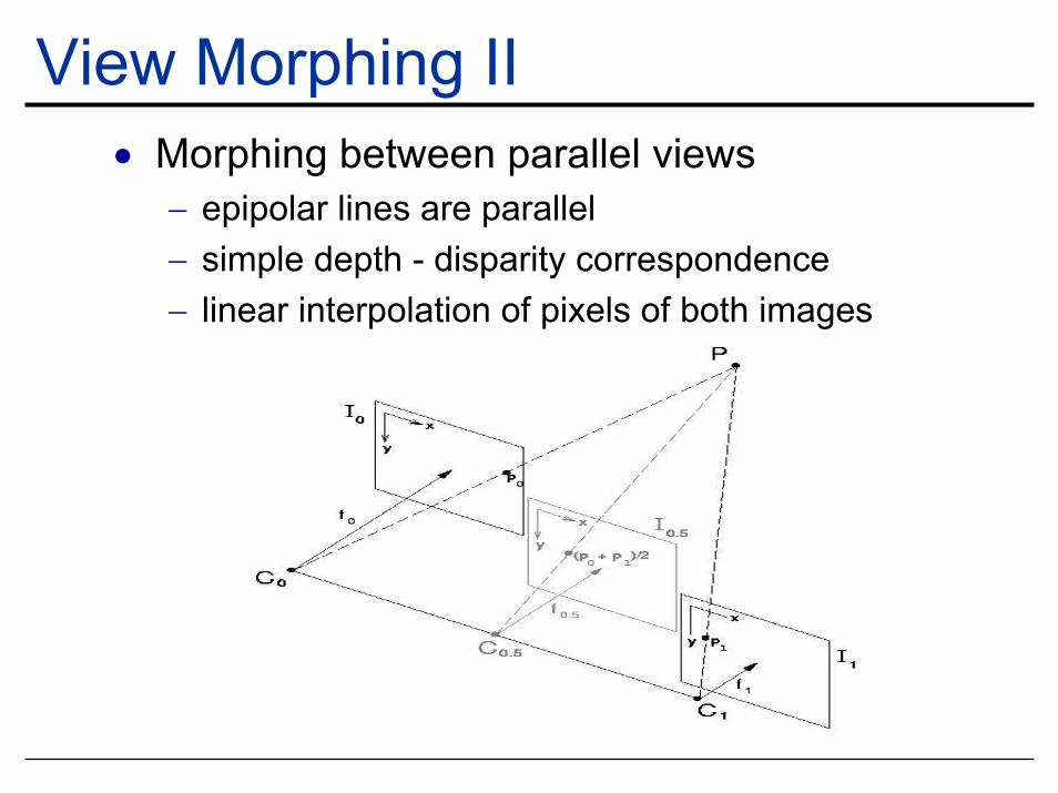
View Morphing II• Morphing between parallel views

− epipolar lines are parallel− simple depth - disparity correspondence− linear interpolation of pixels of both images

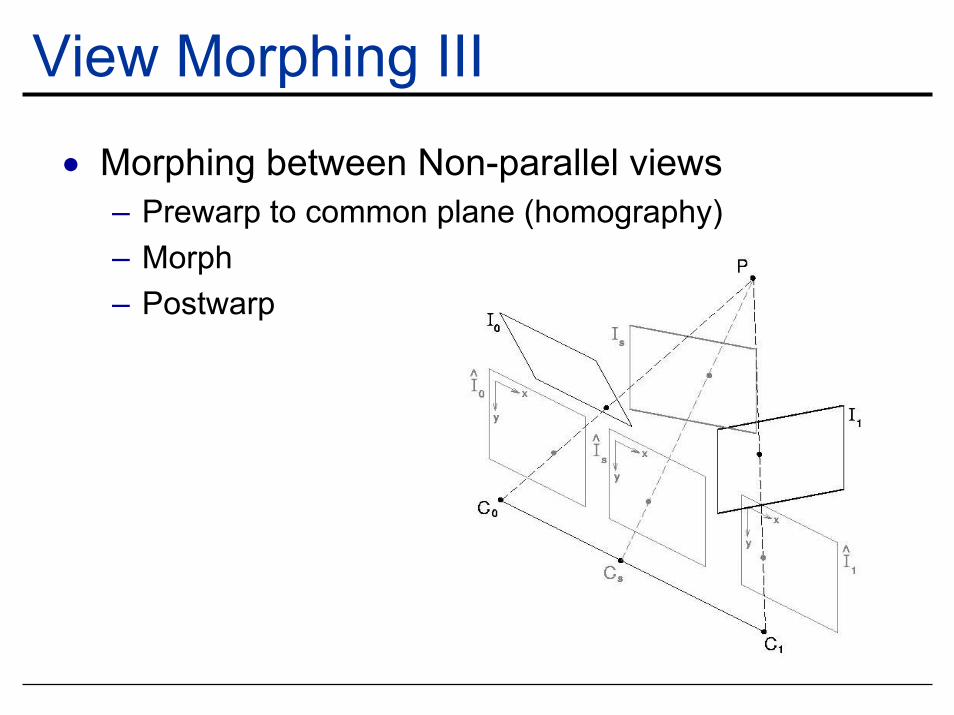
View Morphing III• Morphing between Non-parallel views

– Prewarp to common plane (homography)– Morph– Postwarp

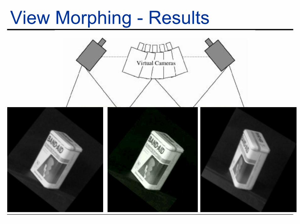
View Morphing - Results

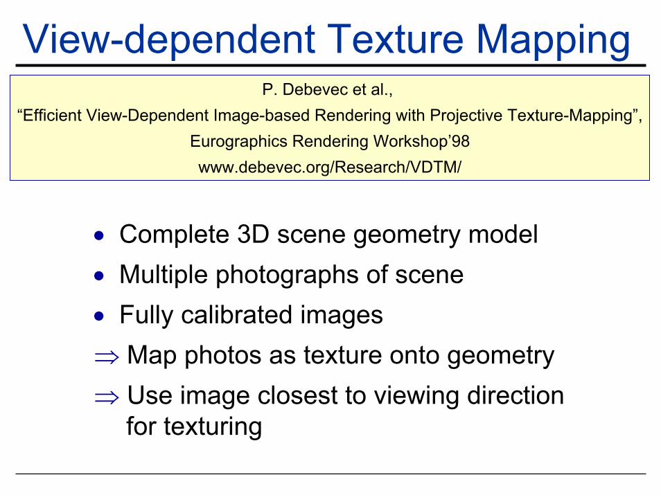
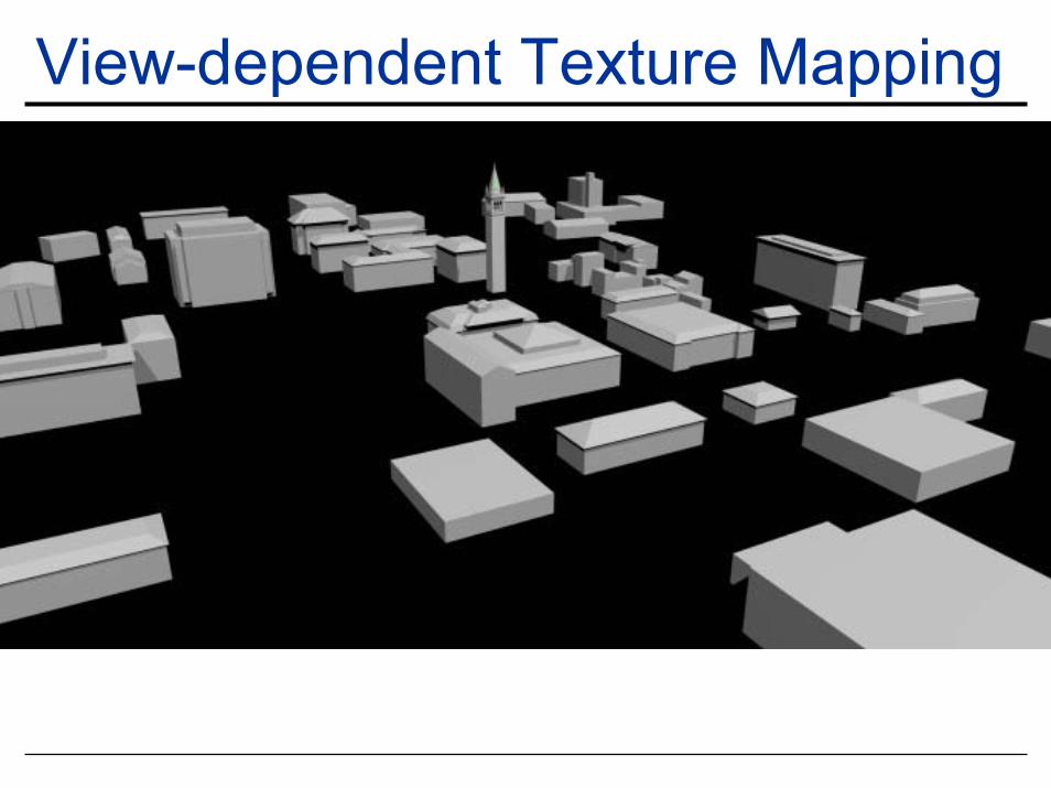
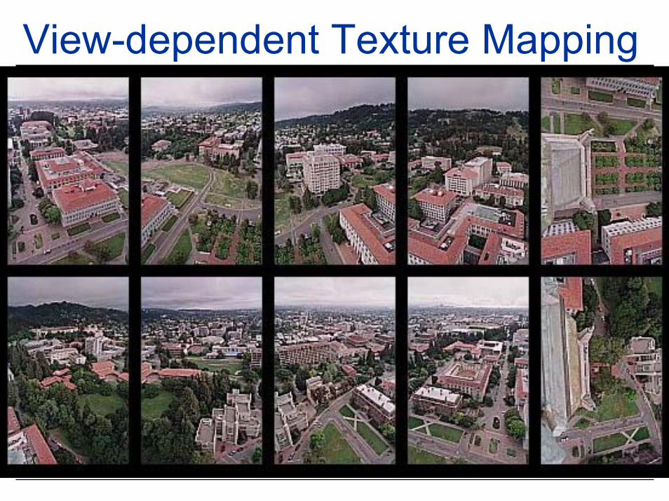
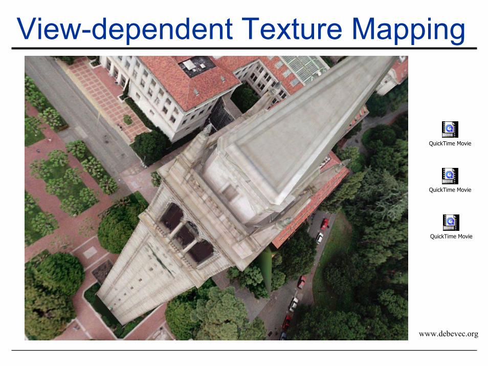
View-dependent Texture MappingP. Debevec et al.,

“Efficient View-Dependent Image-based Rendering with Projective Texture-Mapping”,Eurographics Rendering Workshop’98www.debevec.org/Research/VDTM/

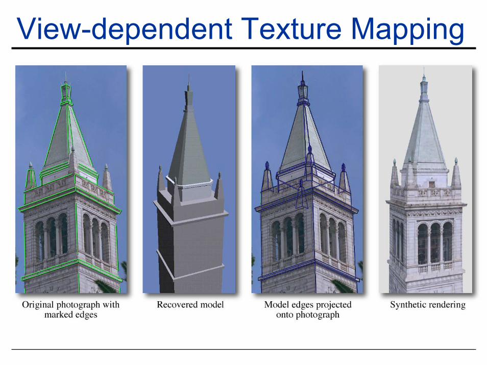
• Complete 3D scene geometry model• Multiple photographs of scene• Fully calibrated images⇒ Map photos as texture onto geometry⇒ Use image closest to viewing direction

for texturing

View-dependent Texture Mapping

View-dependent Texture Mapping

View-dependent Texture Mapping

View-dependent Texture Mapping

QuickTime Movie

QuickTime Movie

QuickTime Movie

www.debevec.org

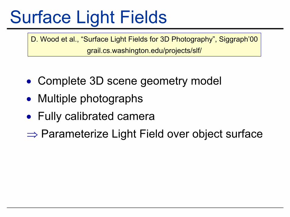
Surface Light FieldsD. Wood et al., “Surface Light Fields for 3D Photography”, Siggraph’00

grail.cs.washington.edu/projects/slf/

• Complete 3D scene geometry model• Multiple photographs• Fully calibrated camera⇒ Parameterize Light Field over object surface

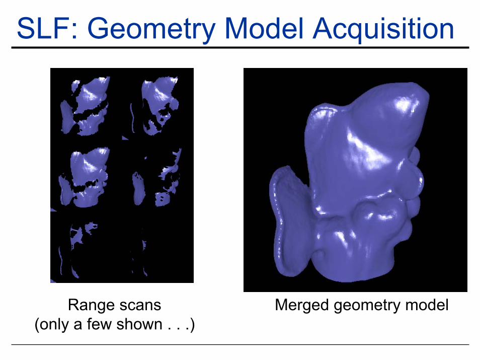
SLF: Geometry Model Acquisition

Range scans(only a few shown . . .)

Merged geometry model

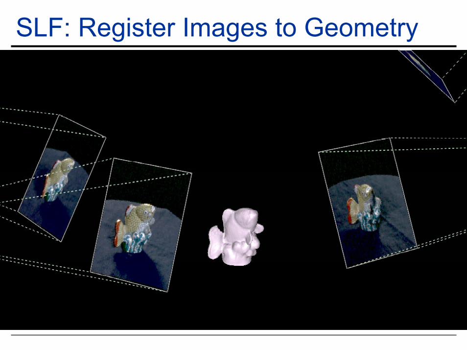
SLF: Register Images to Geometry

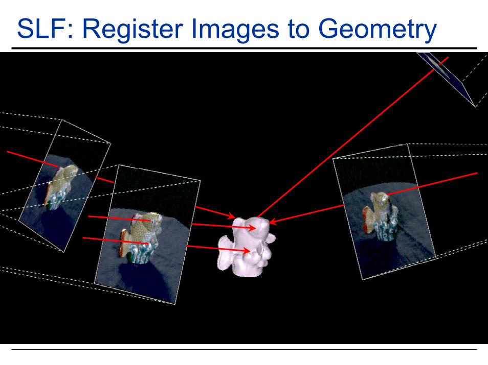
SLF: Register Images to Geometry

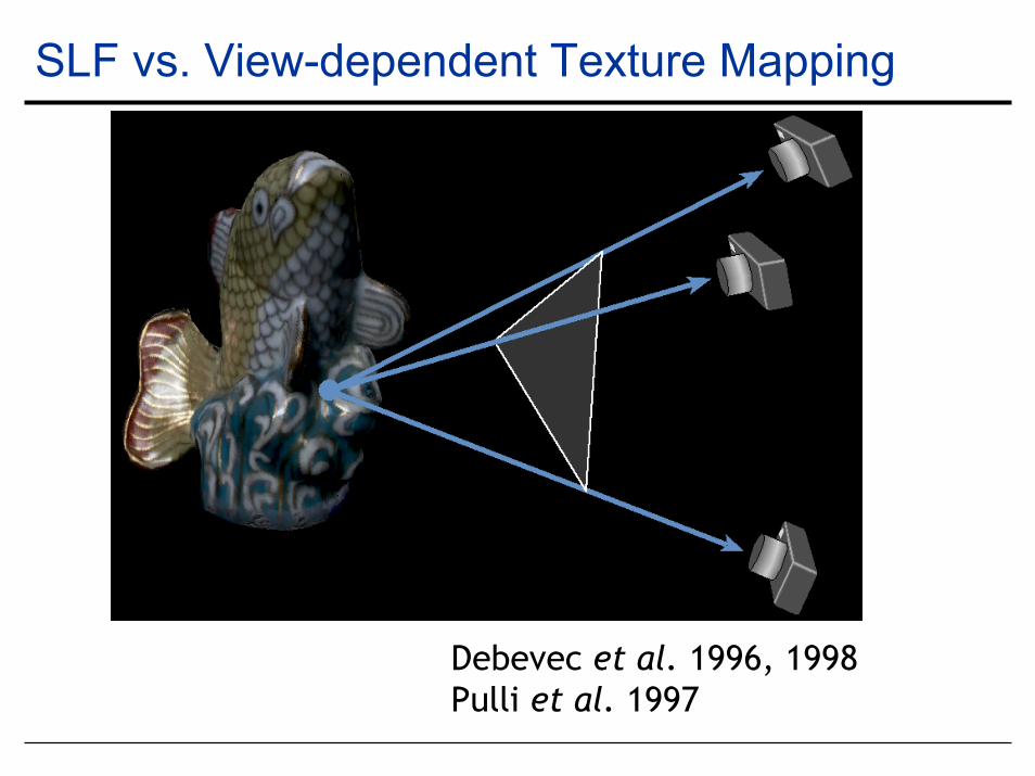
SLF vs. View-dependent Texture Mapping

Debevec et al. 1996, 1998Pulli et al. 1997

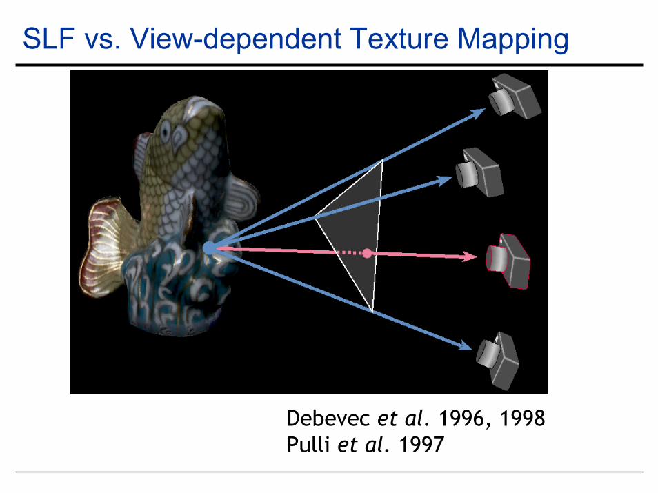
SLF vs. View-dependent Texture Mapping

Debevec et al. 1996, 1998Pulli et al. 1997

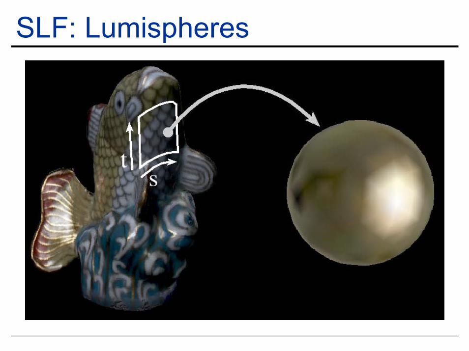
SLF: Lumispheres

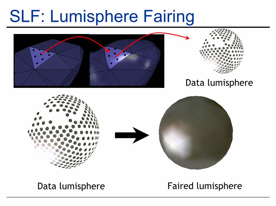
SLF: Lumisphere Fairing

Data lumisphere

Faired lumisphereData lumisphere

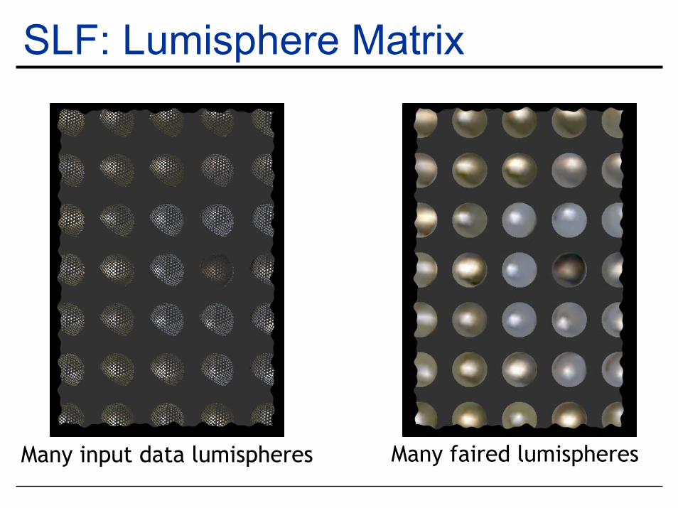
SLF: Lumisphere Matrix

Many faired lumispheresMany input data lumispheres

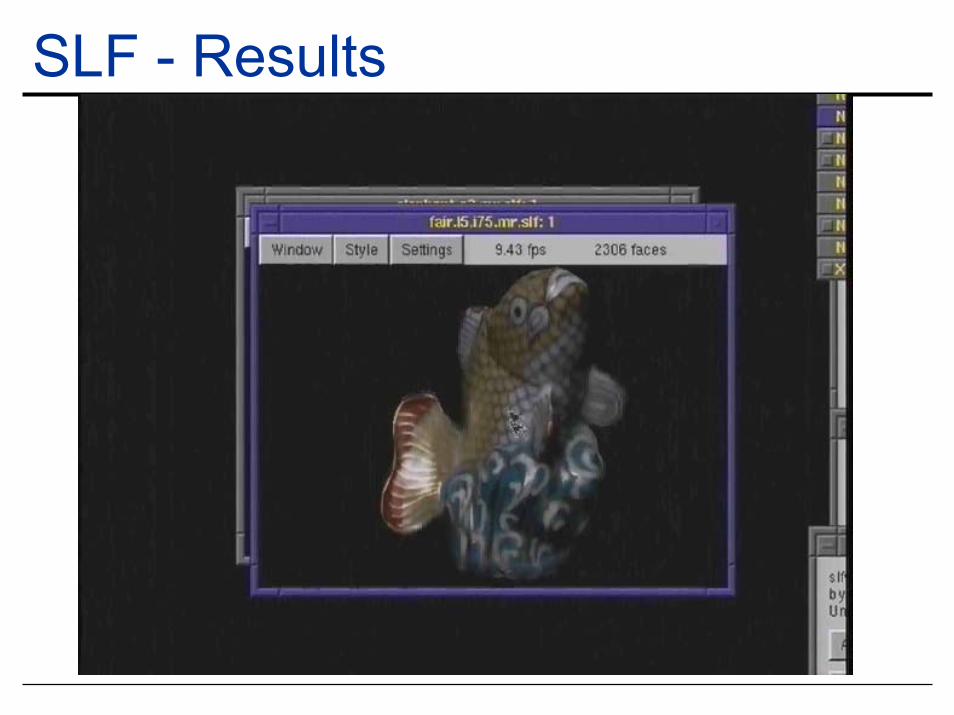
SLF - Results

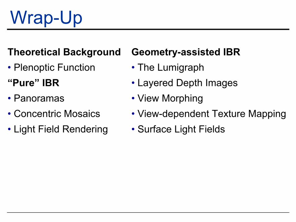
Wrap-Up

Theoretical Background• Plenoptic Function“Pure” IBR• Panoramas• Concentric Mosaics• Light Field Rendering

Geometry-assisted IBR• The Lumigraph• Layered Depth Images• View Morphing• View-dependent Texture Mapping• Surface Light Fields