Computer Graphics: An Implementor’s Guide

Luther A. Tychonievich

May 5, 2008 – March 8, 2010

This work is licensed under the Creative CommonsAttribution-Noncommercial-Share Alike 3.0 United States Li-cense. To view a copy of this license, visit

http://creativecommons.org/licenses/by-nc-sa/3.0/us/

or send a letter to

Creative Commons171 Second Street, Suite 300San Francisco, CA 94105USA

Preface

Although only marginally interested in this subject, I wasa teaching assistant for Brigham Young University’s senior-level computer graphics class for four years, working withtwo professors and several hundred students. That experi-ence taught me that most students misunderstand the samethings. This booklet is designed to present ideas in such away that those particular problems will not arise.

I am aware that the pedagogy and terminology in thisbooklet are not always those commonly in use. There aretopics that people ought to know which are not here, andothers that are breezed over rather glibly without citing thepeople who spent years of their lives developing the tech-niques discussed. This is intentional; my goal is to presentideas in a way that is accessible and leads to implementa-tions which are easy to understand and maintain. I find thatciting papers makes simple ideas seem less accessible to mostundergraduates, and the most optimal solutions possible isusually a lot more brittle and difficult to get working thanare slightly less optimal but much cleaner versions.

It is also possible that some things I say are just plainfalse. As I said, I am only marginally interested in graphicsand have not researched much of this. I have tried most ofit out myself and proven many facts to my own satisfaction,but anyone who still thinks proofs or testing validates analgorithm has not yet written enough algorithms. That said,I am not intentionally misleading and will happily correcterrors or clarify misleading points if they are identified tome.

—Luther TychonievichM.S. in Computer Science, BYU, 2008

lty@cs.byu.edu

i

Contents

1 Rasterization: Idea → Screen 11.1 Introduction to Rasterization . . . . . . . . . 11.2 Normalized Device Coordinates → Device Co-

ordinates . . . . . . . . . . . . . . . . . . . . 11.3 Terminology: vector 6= vector . . . . . . . . . 21.4 Rasterizing a Line Segment . . . . . . . . . . 2

1.4.1 DDA Line Drawing . . . . . . . . . . . 31.4.2 DDA Grid Walking . . . . . . . . . . . 3

1.5 Polygon Contents . . . . . . . . . . . . . . . . 41.6 Extensions of DDA . . . . . . . . . . . . . . . 5

1.6.1 Perspective-correct Interpolation . . . 51.6.2 DDA-like technique for Polynomials . 61.6.3 Drawing Implicit Curves . . . . . . . . 71.6.4 Just Integers, No Division . . . . . . . 81.6.5 About Names . . . . . . . . . . . . . . 81.6.6 Example: Midpoint Circle Algorithm . 8

1.7 Fragment Shading: All the Per-Pixel Details . 91.8 Rasterization-time clipping . . . . . . . . . . 10

2 Raytracing: Screen → Idea 122.1 Introduction to Raytracing . . . . . . . . . . 12

2.2 Primary and Secondary Rays . . . . . . . . . 12

2.3 Rays and Ray-* Intersections . . . . . . . . . 13

2.3.1 Ray-Plane Intersection . . . . . . . . . 13

2.3.2 Ray-Sphere Intersection . . . . . . . . 13

2.3.3 Ray-AABB Intersection . . . . . . . . 14

2.4 Inverse Mapping and Barycentric Coordinates 14

2.4.1 Inverse Sphere Mapping . . . . . . . . 14

2.4.2 Inverse Triangle Mapping . . . . . . . 14

2.5 Direct Illumination . . . . . . . . . . . . . . . 15

2.5.1 Ambient Light . . . . . . . . . . . . . 16

2.5.2 Diffuse Light . . . . . . . . . . . . . . 16

2.5.3 Specular Light . . . . . . . . . . . . . 16

2.6 Secondary Rays . . . . . . . . . . . . . . . . . 17

2.6.1 Shadows . . . . . . . . . . . . . . . . . 17

2.6.2 Reflection . . . . . . . . . . . . . . . . 17

2.6.3 Transparency . . . . . . . . . . . . . . 17

2.6.4 Global Illumination . . . . . . . . . . 18

2.7 Photon Mapping and Caustics . . . . . . . . 18

2.8 Sub-, Super-, and Importance-Sampling . . . 18

ii

Chapter 1

Rasterization: Idea → Screen

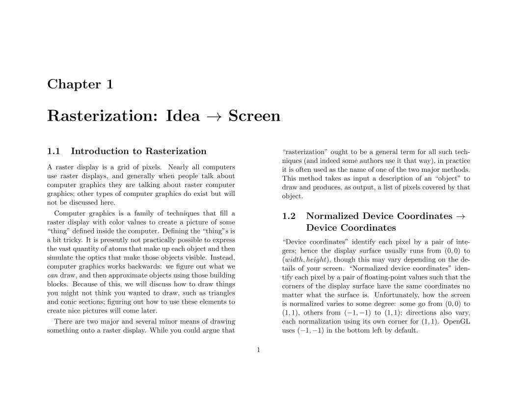
1.1 Introduction to Rasterization

A raster display is a grid of pixels. Nearly all computersuse raster displays, and generally when people talk aboutcomputer graphics they are talking about raster computergraphics; other types of computer graphics do exist but willnot be discussed here.

Computer graphics is a family of techniques that fill araster display with color values to create a picture of some“thing” defined inside the computer. Defining the “thing”s isa bit tricky. It is presently not practically possible to expressthe vast quantity of atoms that make up each object and thensimulate the optics that make those objects visible. Instead,computer graphics works backwards: we figure out what wecan draw, and then approximate objects using those buildingblocks. Because of this, we will discuss how to draw thingsyou might not think you wanted to draw, such as trianglesand conic sections; figuring out how to use these elements tocreate nice pictures will come later.

There are two major and several minor means of drawingsomething onto a raster display. While you could argue that

“rasterization” ought to be a general term for all such tech-niques (and indeed some authors use it that way), in practiceit is often used as the name of one of the two major methods.This method takes as input a description of an “object” todraw and produces, as output, a list of pixels covered by thatobject.

1.2 Normalized Device Coordinates →Device Coordinates

“Device coordinates” identify each pixel by a pair of inte-gers; hence the display surface usually runs from (0, 0) to(width, height), though this may vary depending on the de-tails of your screen. “Normalized device coordinates” iden-tify each pixel by a pair of floating-point values such that thecorners of the display surface have the same coordinates nomatter what the surface is. Unfortunately, how the screenis normalized varies to some degree: some go from (0, 0) to(1, 1), others from (−1,−1) to (1, 1); directions also vary,each normalization using its own corner for (1, 1). OpenGLuses (−1,−1) in the bottom left by default.

1

You can get OpenGL emulate device coordinate by call-ing something like the following anytime the window changessize:

void resize(width, height) {

glViewport(0, width, 0, height);

glMatrixMode(GL_PROJECTION); glLoadIdentity();

glMatrixMode(GL_MODELVIEW); glLoadIdentity();

glOrtho(0, width, 0, height, -1, 1);

}

Then you can access a pixel x, y with color r, g, b(where 1 is full intensity) by glColor3f(r, g, b);

glVertex2f(x, y);.

If you are using a 2D graphics library, there is probablysome function like setPixel(x,y,color) which also acceptsdevice coordinates.

If yn is a normalized coordinate, ys0 is the minimal pixel y(usually 0), and ys1 is the maximal pixel y (usually the heightof the window), the point-point line formula allows us to con-vert between normalized and non-normalized coordinates:

(ys − ys0)(yn1 − yn0) = (yn − yn0)(ys1 − ys0).

1.3 Terminology: vector 6= vector

Computer graphics uses several different sub-disciplines ofmathematics, which creates a few namespace collisions. Someof these I’ll cleverly ignore, as the contexts are sufficientlydifferent not to cause confusion. One we need to make explicitif the term “vector.” In linear algebra a vector is an elementof a vector space and, for our purposes, can be expressed as

a finite ordered list of real numbers:

~x , (x1, x2, . . . , xn)

~x+ ~y , (x1 + y1, x2 + y2, . . . , xn + yn)

~x− ~y , (x1 − y1, x2 − y2, . . . , xn − yn)

~x⊗ ~y , (x1 × y1, x2 × y2, . . . , xn × yn)

s~x , ~x× s , (x1 × s, x2 × s, . . . , xn × s)

~x÷ s , (x1 ÷ s, x2 ÷ s, . . . , xn ÷ s)

In geometry, there are several different uses of mathemati-cal vectors, unfortunately including both Euclidean vectorsand homogeneous vectors, all commonly called “vectors”, aswell as Euclidean and homogeneous points. There is, to myknowledge, no commonly accepted notation for distinguishingbetween these, so I will introduce my own: −→x for a Euclideanvector, −→x h for a homogeneous vector, x for a Euclidean point,and xh for a homogeneous point.Throughout this chapter (except as noted), everything we

know about a point we will dump into one big vector; for ex-ample, if we know position x, y, z, normal nx, ny, nz, colorr, g, b, opacity α, and texture coordinates u, v we have a12-vector for the point ~p = (x, y, z, nx, ny, nz, r, g, b, α, u, v).

1.4 Rasterizing a Line Segment

Suppose you have a line from ~p0 to ~p1 that you want to dis-play. The mathematically correct solution to this problemwould be a blank screen—mathematical lines have no widthand cannot be seen. What we want instead is either (1) acontiguous set of pixels which approximate the line or (2)the set of all the pixels through which the line passes. Thefirst problem is easier, so we’ll address it first.

2

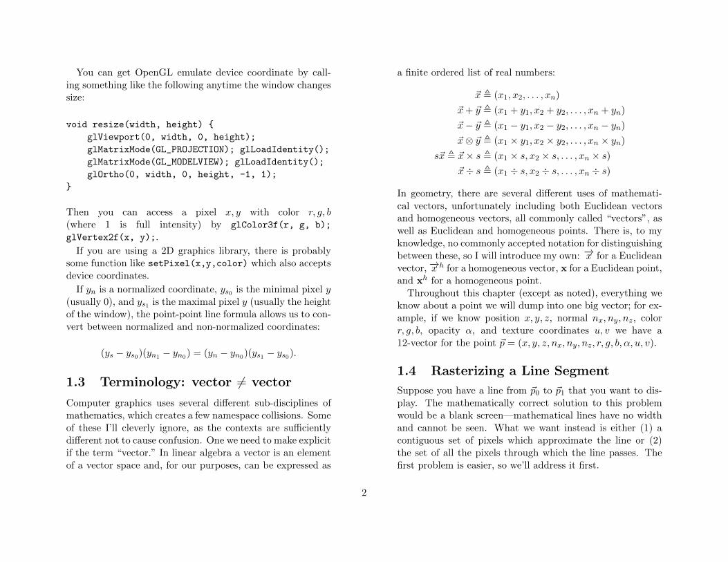
∆~p~p1

~p2

d~p0

d~p

Figure 1.1: Rasterization of a line. Pixel locations are representedby dots; filled pixels by squares.

1.4.1 DDA Line Drawing

We here present a version of the Digital Differential Analyzer(DDA) line drawing algorithm, which draws a contiguous setof pixels approximating a line. By contiguous we mean that,for mostly horizontal lines, there is one pixel per column ofpixels; for mostly vertical lines we want one pixel per row ofpixels instead. This leads to the following algorithmic outline:

1. figure out if we step columns or rows,2. find an increment to get from one column/row to the

next,3. find the first column/row, and4. use the increment and rounding to generate all the pixels.

This process is illustrated at a high level in Figure 1.1, givenformally in Algorithm 1.1, and discussed in more detail below.

Let’s assume we have the two endpoints ~p1 and ~p2. First,we find the vector separating the endpoints, ∆~p = ~p2− ~p1. If∆~p’s x has a larger absolute value than its y, we step columns;otherwise we step rows. Let i be the index of that value; that

is ∆pi = x if we are stepping columns, ∆pi = y if we arestepping rows. Let j be the index of the other xy coordinate.

If ∆pi is negative, swap ~p1 and ~p2, which causes everyelement in ∆~p to be negated.

The increment to move between pixels, d~p, must have thesame direction as ∆~p, but should be length 1 in the i direc-tion. This is trivially created by dividing by the length wehave:

d~p =∆~p

∆pi

To find the first pixel, we want to round the ith compo-nent of ~p1 to the nearest pixel value. If we do this directly,however, we will generally change what line we draw, so weneed to tweak the other coordinates as well. This is easy todo, however; if we want to change ~p1 i by r we can simply addrd~p to ~p1. This observation results in

d~p0 = (dp1 ie − p1 i) d~p.

Now you want to draw the nearest pixel to the points~p1 + d~p0, ~p1 + d~p0 + d~p, ~p1 + d~p0 + 2d~p, etc., up to but notincluding ~p2. If you do include ~p2 then two lines sharing acommon end-point might both fill that point, which is slightlyinefficient and can create problems with transparency.

1.4.2 DDA Grid Walking

Sometimes we want to find all the pixels a line passes throughinstead of just an approximation. Given a particular ~q, theline may pass through both dqje and bqjc, or it may passthrough only one of them. If it passes through two then thepoint where the line passes between the two pixels is given

3

Algorithm 1.1 Basic DDA Algorithm

Input: points ~p1 and ~p2 in device coordinatesPurpose: draw a line conneting ~p1 and ~p21: ∆~p ⇐ ~p2 − ~p12: if |∆px| > |∆py| then — step in columns

3: i ⇐ indexof(x)4: j ⇐ indexof(y)5: else — step in rows

6: i ⇐ indexof(y)7: j ⇐ indexof(x)8: if ∆pi < 0 then9: swap ~p1 and ~p2

10: ∆~p ⇐ −∆~p11: d~p ⇐ ∆~p÷∆pi12: d~p0 = (dp1 ie − p1 i) d~p13: ~q ⇐ ~p1 + d~p014: while qi < p2 i do — note “<”, not “≤”

15: — note qi is already an integer; only qj needs to be

rounded. . .

16: plotPixel(round(qx), round(qy), qcolor)17: ~q ⇐ ~q + d~p

by the intersection of j = bqjc+ 0.5 and the line:

qi +0.5− qj + bqjc

dqj;

if this number is more than 0.5 away from qi then the lineonly passes through one pixel.This observation creates the following modification of Al-

gorithm 1.1: replace line 16 with

offset ⇐ 0.5−qj+bqjcdqj

if |offset| < 0.5 thenplotPixel(bqxc), bqyc, qcolor)plotPixel(dqxe), dqye, qcolor)

elseplotPixel(round(qx), round(qy), qcolor)

You can also use the offset information to created an anti-aliased line; I’ll leave this as an exercise for the reader.

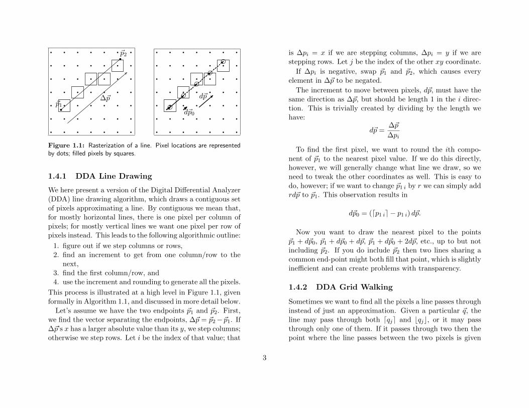
1.5 Polygon Contents

To fill the pixels contained within a polygon, we use the DDAalgorithm first in y along the edges, then in x between them.This really is the entirety of the polygon fill, as illustrated inFigure 1.2 and made formal in Algorthim 1.2.Note that rasterizing a triangle works very nicely, but ras-

terizing other shapes is a bit of a misnomer. You can usethe double DDA technique listed here for any polygon—we’lldiscuss how momentarily—but if not all the vertices are thesame color this can create some really strange looking results.That said, people often ask for arbitrary polygons to be

filled. For rasterizing, either split them into triangles or usethe DDA technique along with what is called the “edge ta-ble.” An edge table is just a list of edges, where an edge is a

4

Figure 1.2: Rasterization of a polygon by first DDA-stepping up theedges, then DDA-stepping between the edges. In Algorithm 1.2, thisimage corresponds to being halfway through the DDA-line call on thefirst iteration of the loop at line 9.

pair of connected vertices. The “global edge table” is the listof all edges in the polygon. The “active edges” for a givenvalue of y are the edges which cross that y. If you consider anedge to include its bottom endpoint’s y but not its top, andignore horizontal edges completely, then every y must havean even number of active edges.

The algorithm then runs as follows.

1. Begin at the smallest y in the polygon.2. DDA up all active edges, of which there are always an

even number.3. At each y, DDA will give you a point for each active

edge. Sort these in x, then DDA between pairs of points(1st and 2nd, 3rd and 4th, etc.).

Algorithm 1.2 Double-DDA Triangle Fill

Input: points ~pb, ~pm, and ~pt in device coordinatesPurpose: draw all pixels inside the triangle1: assert(pb y ≤ pm y ≤ pt y)2: Find d~p and initial ~q for (~pb, ~pm); call them d~pa and ~qa3: Find d~p and initial ~q for (~pb, ~pt); call them d~pc and ~qc4: while ~qa y < pm y do5: DDA-Line(~qa, ~qc)6: (~qa, ~qc) ⇐ (~qa + d~qa, ~qc + d~qc)7: Find d~p and initial ~q for (~pm, ~pt); call them d~pe and ~qe8: while ~qe y < pt y do9: DDA-Line(~qe, ~qc)

10: (~qe, ~qc) ⇐ (~qe + d~qe, ~qc + d~qc)

1.6 Extensions of DDA

The basic DDA-based line and polygon drawing routines areelegant and efficient, but are rather restricted in their appli-cation. This section lists a number of extensions, some verycommon, others more unusual.

1.6.1 Perspective-correct Interpolation

The basic technique discussed above interpolates everythinglinearly, which is great for 2D drawing, but for perspectivedrawing it does not preserve interiors of objects correctly (seeFigure 1.3). Fortunately, there is a simple fix which uses lin-ear interpolation to create perspective-correct results. Thetheory behind this method was first published in Jim Blinn’s1992 “Hyperbolic Interpolation” and is cleanly explained inKok-Lim Low’s 2002 paper “Perspective-Correct Interpola-tion,” which is freely available online. I present only the

5

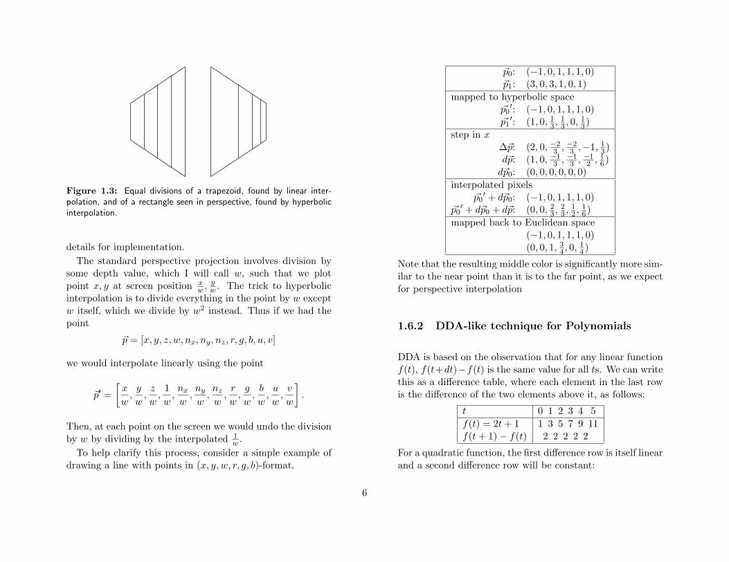
Figure 1.3: Equal divisions of a trapezoid, found by linear inter-polation, and of a rectangle seen in perspective, found by hyperbolicinterpolation.

details for implementation.

The standard perspective projection involves division bysome depth value, which I will call w, such that we plotpoint x, y at screen position x

w ,yw . The trick to hyperbolic

interpolation is to divide everything in the point by w exceptw itself, which we divide by w2 instead. Thus if we had thepoint

~p = [x, y, z, w, nx, ny, nz, r, g, b, u, v]

we would interpolate linearly using the point

~p′ =

[x

w,y

w,z

w,1

w,nx

w,ny

w,nz

w,r

w,g

w,b

w,u

w,v

w

].

Then, at each point on the screen we would undo the divisionby w by dividing by the interpolated 1

w .

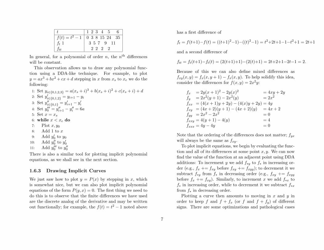
To help clarify this process, consider a simple example ofdrawing a line with points in (x, y, w, r, g, b)-format.

~p0: (−1, 0, 1, 1, 1, 0)~p1: (3, 0, 3, 1, 0, 1)

mapped to hyperbolic space~p0

′: (−1, 0, 1, 1, 1, 0)~p1

′: (1, 0, 13 ,13 , 0,

13)

step in x∆~p: (2, 0, −2

3 , −23 ,−1, 13)

d~p: (1, 0, −13 , −1

3 , −12 , 16)

d~p0: (0, 0, 0, 0, 0, 0)

interpolated pixels~p0

′ + d~p0: (−1, 0, 1, 1, 1, 0)~p0

′ + d~p0 + d~p: (0, 0, 23 ,23 ,

12 ,

16)

mapped back to Euclidean space(−1, 0, 1, 1, 1, 0)(0, 0, 1, 34 , 0,

14)

Note that the resulting middle color is significantly more sim-ilar to the near point than it is to the far point, as we expectfor perspective interpolation

1.6.2 DDA-like technique for Polynomials

DDA is based on the observation that for any linear functionf(t), f(t+dt)−f(t) is the same value for all ts. We can writethis as a difference table, where each element in the last rowis the difference of the two elements above it, as follows:

t 0 1 2 3 4 5

f(t) = 2t+ 1 1 3 5 7 9 11f(t+ 1)− f(t) 2 2 2 2 2

For a quadratic function, the first difference row is itself linearand a second difference row will be constant:

6

t 1 2 3 4 5 6

f(t) = t2 − 1 0 3 8 15 24 35ft 1 3 5 7 9 11ftt 2 2 2 2

In general, for a polynomial of order n, the nth differenceswill be constant.This observation allows us to draw any polynomial func-

tion using a DDA-like technique. For example, to ploty = ax3 + bx2 + cx+ d stepping in x from xs to xe we do thefollowing:

1: Set yi∈{0,1,2,3} = a(xs + i)3 + b(xs + i)2 + c(xs + i) + d2: Set y′i∈{0,1,2} = yi+1 − yi3: Set y′′i∈{0,1} = y′i+1 − y′i4: Set y′′′0 = y′′i+1 − y′′i = 6a5: Set x = xs6: while x < xe do7: Plot x, y08: Add 1 to x9: Add y′0 to y0

10: Add y′′0 to y′011: Add y′′′0 to y′′0There is also a similar tool for plotting implicit polynomialequations, as we shall see in the next section.

1.6.3 Drawing Implicit Curves

We just saw how to plot y = P (x) by stepping in x, whichis somewhat nice, but we can also plot implicit polynomialequations of the form P (y, x) = 0. The first thing we need todo this is to observe that the finite differences we have usedare the discrete analog of the derivative and may be writtenout functionally; for example, the f(t) = t2 − 1 noted above

has a first difference of

ft = f(t+1)−f(t) = ((t+1)2−1)−((t)2−1) = t2+2t+1−1−t2+1 = 2t+1

and a second difference of

ftt = ft(t+1)−ft(t) = (2(t+1)+1)−(2(t)+1) = 2t+2+1−2t−1 = 2.

Because of this we can also define mixed differences asfxy(x, y) = fx(x, y + 1)− fx(x, y). To help solidify this idea,consider the differences for f(x, y) = 2x2y:

fx = 2y(x+ 1)2 − 2y(x)2 = 4xy + 2yfy = 2x2(y + 1)− 2x2(y) = 2x2

fxx = (4(x+ 1)y + 2y)− (4(x)y + 2y) = 4yfxy = (4x+ 2)(y + 1)− (4x+ 2)(y) = 4x+ 2fyy = 2x2 − 2x2 = 0fxxy = 4(y + 1)− 4(y) = 4fxxx = 4y − 4y = 0

Note that the ordering of the differences does not matter; fyxwill always be the same as fxy.To plot implicit equations, we begin by evaluating the func-

tion and all of its differences at some point x, y. We can nowfind the value of the function at an adjacent point using DDAadditions: To increment y we add f∗y to f∗ in increasing or-der (e.g., fx += fxy before fxy += fxyy); to decrement it wesubtract f∗y from f∗ in decreasing order (e.g., fxy += fxyybefore fx += fxy). Similarly, to increment x we add f∗x tof∗ in increasing order, while to decrement it we subtract f∗xfrom f∗ in decreasing order.Plotting a curve then amounts to moving in x and y in

order to keep f and f + fx (or f and f + fy) of differentsigns. There are some optimizations and pathological cases

7

as well; see Van Aken & Novak, “Curve-drawing algorithmsfor raster displays” ACM TOG (April 1985) pp. 147–169 fora discussion.

1.6.4 Just Integers, No Division

We can pose the DDA technique without any division, andif we do we can also draw shapes with integer inputs us-ing only integer math. To do this, notice for a DDA linestepping in y, the denominator of all coordinates is ∆y.Thus, given x = a b

∆y on one row, where a = bxc, on

the next row it is x′ = a + b+∆x∆y . Let i = ∆x ÷ ∆y

and r = ∆x (mod ∆y) and we can rewrite that as x′ =(a+i)+ b+r

∆y . This allows the following method for increment-ing y:

1: Set b = b+ r2: Set a = a+ i3: if b ≥ ∆y then4: Set a = a+ 15: Set b = b−∆y

If no division is available, we can alsowrite

1: Set a = a+∆x2: while b ≥ ∆y do3: Set a = a+ 14: Set b = b−∆y

For software running on modern PC hardware, this methodof avoiding divisions has little perceptible runtime differencefrom the straight DDA on floating-point data. However, forsimpler embedded processors or custom-made hardware it isnoticeably faster, and in all cases it avoids the roundoff errorpresent in floating-point DDA.

1.6.5 About Names

We have discussed the DDA algorithm in vector form be-cause that seems to be the cleanest version to understand. Ingraphics literature, DDA is usually presented in an element-by-element form instead; DDA-based polygon fill is calledlinear scan-line interpolation (and often presented withoutthat d~p0s, an omission that causes neighboring polygons tooverlap), and the integer-only technique for lines is called theBresenham line algorithm. The implicit curve plotting rou-tine was published as the midpoint algorithm, named afteran optimization where the next pixel is analytically reducedto one of two pixels and the sign at the midpoint of the twois used to pick which one to plot.

1.6.6 Example: Midpoint Circle Algorithm

This example walks through using the implicit DDA in theinteger-only form with some additional optimizations, to-gether known as the midpoint circle algorithm.

The goal is to draw a circle, centered at the origin, withradius r. We first note that it suffices to draw an eighthof the circle, since by symmetry we know that if we plotpixel (x, y) we will also plot pixels (−x, y), (−x,−y), (x,−y),(y, x), (−y, x), (−y,−x), and (y,−x). We will pick, arbitrar-ily, to generate points on the top half of the left side of thecircle, where 0 ≤ y ≤ −x; the rest of the circle we will createusing symmetry.

The implicit equation of a circle is P (x, y) = x2+y2−r2 =0. We will start at the point (−r, 0), since we know it is one we

8

want to plot, and find the following initial finite differences:

P (−r, 0) = 0

Px(−r, 0) = [2x+ 1]x=−r = −2r + 1

Py(−r, 0) = [2y + 1]y=0 = 1

Pxx = Pyy = 2;

all the other differences are zero. This is enough to writea basic form of the algorithm, Algorithm 1.3: Note that we

Algorithm 1.3

Input: Integer radius rPurpose: Plot the interior border of the circle1: (x, y) ⇐ (−r, 0)2: P ⇐ 03: (Px, Py) ⇐ (−2r + 1, 1)4: (Pxx, Pxy, Pyy) ⇐ (2, 0, 2)5: while y < −x do6: Plot the eight points (±x,±y),(±y,±x)7: Increment y8: Add Py to P9: Add Pyy to Py

10: if P > 0 then11: Increment x12: Add Px to P13: Add Pxx to Px

do not need a while loop for incrementing x because in theregion we selected, the slope never drops below one, so foreach step x either stays the same or increments exactly once.This code is both efficient and accurate as long as you only

wish to color pixels inside the circle. Often, however, people

want to color the pixels that are as close to the boundaryas possible; this is done using the “midpoint” version of thealgorithm. The idea is simple; instead of finding the initialvalue of P at the first pixel, we find the value at the midpointof the first pixel and the next pixel outward from it; that is,P (−r− 1

2 , 0) = −r− 14 and Px(−r− 1

2 , 0) = −2r. We can getrid of the 1

4 by observing that if P = 0 then 4P must alsoequal zero, giving us initial values of

P = −r − 1

Px = −8r

Py = 4

Pxx = Pyy = 8.

If we plug these directly into the algorithm presented earlier,we will be evaluating the polynomial at the midpoint betweentwo pixels (hence the name “midpoint algorithm”) and plotthose pixels closest to the actual circle itself.

1.7 Fragment Shading: All thePer-Pixel Details

So far we have discussed how to use the mathematical de-scription of an object to generate a set of pixels, each witha color, position, normal, and whatever else you want to in-terpolate. In real-time graphics each of these pixels is calleda fragment and the code that translates them into color onthe screen is called the fragment shader. Fragment shadersare nice because their runtime performance is dictated bythe number of pixels on the screen rather than the numberof polygons displayed.

The simplest fragment shader sets the color of the pixel on

9

the screen to be the color interpolated to the fragment.

Usually, people use depth buffering to draw only the clos-est fragment at each pixel. Do do this, simply create storea depth value for each pixel. Then, for each fragment, if itsdepth is closer than the stored depth, draw it and updatethe stored depth; otherwise, discard it. This is called depth-buffering or z-buffering.

You can also light each pixel individually. This processis called Phong shading (not to be confused with Phonglighting) or per-pixel lighting. Phong shading takes asinput the interpolated object color, pre-device-coordinate-transform vertex position, and vertex normal of a fragment.These are combined using your favorite lighting model (seeSection 2.5) to find the color to plot. Note that applying alighting model to the vertices and interpolating the lit coloris called Gouraud shading; most graphics cards default toGouraud shading.

Texture mapping is done by interpolating texture coordi-nates to each fragment and looking up the appropriate colorfrom a texture image. Typically, texture coordinates arespecified in the range [0, 1) so you’ll want to do a device-coordinate-like transformation before doing the texel lookup.There is no reason to restrict textures to storing color infor-mation; bump mapping, stores an offset for the normal inthe texture (which only works if you do Phong shading, sinceGouraud ignores per-fragment normals). Procedural texturesgenerate texture valued through a function rather than viaan image lookup.

Mip-mapping is a way of improving textures by having anumber of versions of the texture stored at different resolu-tions. The resolution selected is based on the magnitude ofthe texture coordinate elements of d~p: larger values means

neighboring texels are farther apart in texture coordinatespace and calls for a lower-resolution texture image. Oftenseveral neighboring texels in several neighboring levels of themip map are combined via some sort of weighted average tocreate a smoother looking scene.

Fog is just a function of the depth of a pixel, like the depthbuffer. More distant fragments have more of their own colorreplaced by the fog color.

It is possible to do transparency in a rasterizing system;just keep part of the existing color on the screen, and blendit with the new fragment’s color. This requires that fragmentsare generated in the right order. Typically, this is done bydrawing all opaque objects first, then sorting the transparentpolygons based on their depth and drawing the most distantones first. Alternately, you can store a linked list of all thefragments on a particular pixel, then sort them and drawthem as a post-processing step. Neither of these techniquesis particularly fast.

1.8 Rasterization-time clipping

You never want to draw pixels off of the screen, both formemory security and speed reasons. There are lots of waysto do clipping, but rasterization-time clipping is the one thatmost graphics cards do.

The naıve version of this is to generate all fragments forall polygons but only plot those that lie within the screenbounds. This is a bad idea; perspective projection often re-sults in polygons hundreds of times larger than the screen,and generating all of those fragments could take a very verylong time; in rare cases floating point roundoff could evencause ~p+ ~dp to be exactly equal to ~p, resulting in an infinite

10

loop.The correct solution here is to modify d~p0 to step not just

to the first row or column of pixels, but all the way to thefirst row or column on the screen. This means we redefine

d~p0 =

{(dp1 ie − p1 i) d~p if p1 i > 0(0− p1 i) d~p otherwise

Similarly, as soon we DDA to the edge of the screen, we canquit. Thus, the adjusted algorithm to only creates on-screenfragments with very little extra work.

11

Chapter 2

Raytracing: Screen → Idea

2.1 Introduction to Raytracing

Raytracing tries to solve the same problem as rasterization—that is, create a set of pixel colors to represent a mathemati-cal description of stuff—but goes about it in reverse. Whererasterization asks the questions “what pixels are containedwithin this object” raytracing asks instead “what objects arevisible within this pixel?” It forms the second major tech-nique of drawing on raster displays.

Raytracing is currently slower than rasterization, thoughit admits almost unlimited amounts of parallelism causingsome people think it will become faster in years to come.Currently its primary advantage is that the process does notdepend on pixel locality and so can easily model reflection,transparency, and similar optical properties.

The speed of a raytracing system depends largely on thequality of the spatial hierarchy used. Conceptually, the ideahere is to collect a group of nearby objects and find a bound-ing box for them; if a box is not visible from a particularpixel, none of the objects within it are either. I will not dis-cuss these hierarchies further, beyond stating that k-d trees

are one of the more popular spatial hierarchies and manydiscussions of k-d trees (and other hierarchies) are availableonline.

2.2 Primary and Secondary Rays

A ray is a semi-infinite line; it is typically stored as a pointcalled the ray origin, ro; and a direction vector −→r d. Thenthe ray itself is the set of points {ro + t−→r d | t ∈ [0,∞)}, andthe goal of raytracing is to find the point in the ray containedwithin another object which is closest to the ray origin (thatis, with minimal t).

Ray tracing creates one or more rays per pixel. Those raysare intersected with objects in the scene and then, generally,several secondary rays are generated from those intersectionpoints, and intersected with the scene again, and then moreare generated, etc., until you get tired of shooting rays, atwhich point you do some sort of direct illumination (see 2.5)and call it good.

There are a number of ways to generate rays from pixels.

12

For all of them we need the camera position and orienta-tion, given by the eye position e and the forward, up, and

right directions−→f , −→u , and −→r ; the ray origin is generally just

e. The most common choice for ray direction is designed toreplicate the standard rasterization perspective look: givennormalized device coordinates for a pixel (x, y), its ray direc-

tion is−→f cos(θ) + (x−→r + y−→u ) sin(θ), where θ is the field of

view. Fish-eye(x−→r + y−→u +

√1− x2 − y2

−→f)and cylindri-

cal(y−→u + cos(x)

−→f + sin(x)−→r

)projections are also used in

some settings.Sections 2.6 and 2.6.4 discusses some of the techniques used

to generate secondary rays.

2.3 Rays and Ray-* Intersections

In general, the intersection of a ray ro + t−→r d with someobject g(p) = 0 is found as the minimal t for whichg(ro + t−→r d) = 0. Constrained minimization of this typeis a widely-studied problem in numerical analysis, optimiza-tion, and many branches of engineering and science. How-ever, most raytracers use only three particular solutions: ray-plane, ray-AABB, and ray-sphere intersections.

2.3.1 Ray-Plane Intersection

Planes can be described in a number of ways; principle amongthem are implicit Ax+By + Cz +D = 0, point-and-normal(−→n , p), and three-point (p0, p1, p2). We will use the point-normal version, noting that

−→n ≡ (A,B,C) ≡ (−−−−−→p1 − p0)× (

−−−−−→p2 − p0)

and that the point(−D

A , 0, 0)is on the plane.

ro −→r d

−−−−→c − ro

p

(−−−→p−ro)·−→n−→r d·−→n

−→rd + ro

−→n

−−−−→p − ro

c

c′c′′

rd

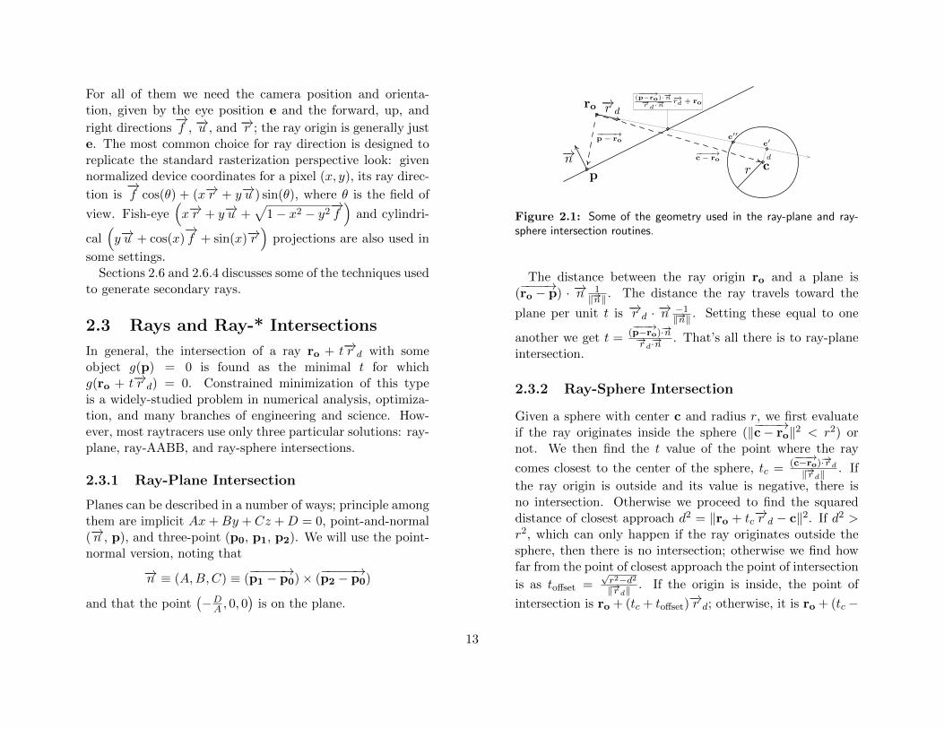
Figure 2.1: Some of the geometry used in the ray-plane and ray-sphere intersection routines.

The distance between the ray origin ro and a plane is(−−−−→ro − p) · −→n 1

‖−→n‖ . The distance the ray travels toward the

plane per unit t is −→r d · −→n −1‖−→n‖ . Setting these equal to one

another we get t = (−−−−→p−ro)·−→n−→r d·−→n

. That’s all there is to ray-planeintersection.

2.3.2 Ray-Sphere Intersection

Given a sphere with center c and radius r, we first evaluateif the ray originates inside the sphere (‖−−−−→c− ro‖2 < r2) ornot. We then find the t value of the point where the ray

comes closest to the center of the sphere, tc = (−−−−→c−ro)·−→r d

‖−→r d‖. If

the ray origin is outside and its value is negative, there isno intersection. Otherwise we proceed to find the squareddistance of closest approach d2 = ‖ro + tc

−→r d − c‖2. If d2 >r2, which can only happen if the ray originates outside thesphere, then there is no intersection; otherwise we find howfar from the point of closest approach the point of intersection

is as toffset =√r2−d2

‖−→r d‖. If the origin is inside, the point of

intersection is ro + (tc + toffset)−→r d; otherwise, it is ro + (tc −

13

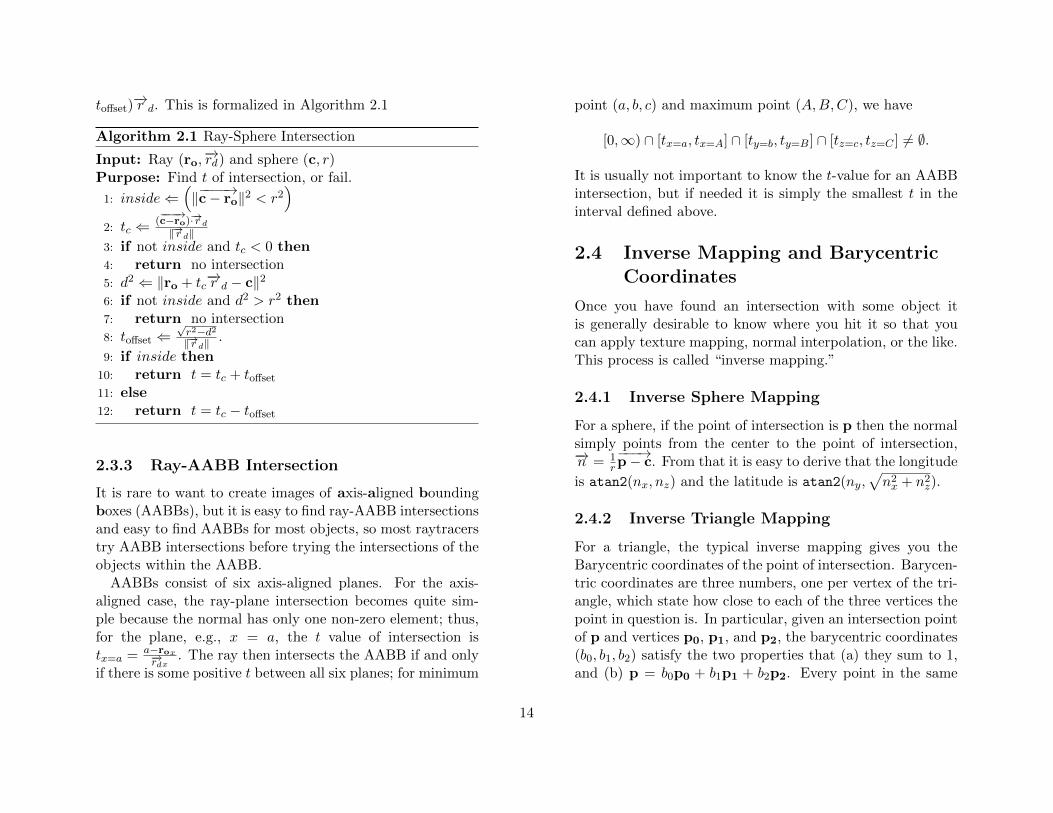
toffset)−→r d. This is formalized in Algorithm 2.1

Algorithm 2.1 Ray-Sphere Intersection

Input: Ray (ro,−→rd) and sphere (c, r)

Purpose: Find t of intersection, or fail.

1: inside ⇐(‖−−−−→c− ro‖2 < r2

)2: tc ⇐ (

−−−−→c−ro)·−→r d

‖−→r d‖3: if not inside and tc < 0 then4: return no intersection5: d2 ⇐ ‖ro + tc

−→r d − c‖26: if not inside and d2 > r2 then7: return no intersection8: toffset ⇐

√r2−d2

‖−→r d‖.

9: if inside then10: return t = tc + toffset11: else12: return t = tc − toffset

2.3.3 Ray-AABB Intersection

It is rare to want to create images of axis-aligned boundingboxes (AABBs), but it is easy to find ray-AABB intersectionsand easy to find AABBs for most objects, so most raytracerstry AABB intersections before trying the intersections of theobjects within the AABB.AABBs consist of six axis-aligned planes. For the axis-

aligned case, the ray-plane intersection becomes quite sim-ple because the normal has only one non-zero element; thus,for the plane, e.g., x = a, the t value of intersection istx=a = a−rox−→rdx

. The ray then intersects the AABB if and onlyif there is some positive t between all six planes; for minimum

point (a, b, c) and maximum point (A,B,C), we have

[0,∞) ∩ [tx=a, tx=A] ∩ [ty=b, ty=B] ∩ [tz=c, tz=C ] 6= ∅.

It is usually not important to know the t-value for an AABBintersection, but if needed it is simply the smallest t in theinterval defined above.

2.4 Inverse Mapping and BarycentricCoordinates

Once you have found an intersection with some object itis generally desirable to know where you hit it so that youcan apply texture mapping, normal interpolation, or the like.This process is called “inverse mapping.”

2.4.1 Inverse Sphere Mapping

For a sphere, if the point of intersection is p then the normalsimply points from the center to the point of intersection,−→n = 1

r

−−−→p− c. From that it is easy to derive that the longitude

is atan2(nx, nz) and the latitude is atan2(ny,√n2x + n2

z).

2.4.2 Inverse Triangle Mapping

For a triangle, the typical inverse mapping gives you theBarycentric coordinates of the point of intersection. Barycen-tric coordinates are three numbers, one per vertex of the tri-angle, which state how close to each of the three vertices thepoint in question is. In particular, given an intersection pointof p and vertices p0, p1, and p2, the barycentric coordinates(b0, b1, b2) satisfy the two properties that (a) they sum to 1,and (b) p = b0p0 + b1p1 + b2p2. Every point in the same

14

p

p0 p1

p2 −→e 2

−→e 1−→e 0

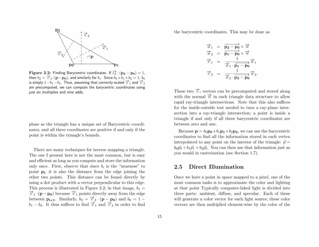
Figure 2.2: Finding Barycentric coordinates. If −→e2 · (p2 − p0) = 1,then b2 = −→e 2 ·(p−p0), and similarly for b1. Since b0+b1+b2 = 1, b0is simply 1−b1−b2. Thus, assuming that correctly-scaled −→e 1 and

−→e 2

are precomputed, we can compute the barycentric coordinates usingjust six multiplies and nine adds.

plane as the triangle has a unique set of Barycentric coordi-nates, and all three coordinates are positive if and only if thepoint is within the triangle’s bounds.

There are many techniques for inverse mapping a triangle.The one I present here is not the most common, but is easyand efficient as long as you compute and store the informationonly once. First, observe that since bi is the “nearness” topoint pi, it is also the distance from the edge joining theother two points. This distance can be found directly byusing a dot product with a vector perpendicular to this edge.This process is illustrated in Figure 2.2; in that image, b1 =−→e 1 · (p−p0) because

−→e 1 points directly away from the edgebetween pi6=1. Similarly, b2 = −→e 2 · (p − p0) and b0 = 1 −b1 − b2. It thus suffices to find −→e 1 and −→e 2 in order to find

the barycentric coordinates. This may be done as

−→a 1 =−−−−−→p2 − p0 ×−→n

−→a 2 =−−−−−→p1 − p0 ×−→n

−→e 1 =1

−→a 1 ·−−−−−→p1 − p0

−→a 1

−→e 2 =1

−→a 2 ·−−−−−→p2 − p0

−→a 2.

These two −→e i vectors can be precomputed and stored alongwith the normal −→n in each triangle data structure to allowrapid ray-triangle intersections. Note that this also sufficesfor the inside-outside test needed to turn a ray-plane inter-section into a ray-triangle intersection; a point is inside atriangle if and only if all three barycentric coordinates arebetween zero and one.

Because p = b0p0+b1p1+b2p2, we can use the barycentriccoordinates to find all the information stored in each vertexinterpolated to any point on the interior of the triangle: ~p =b0 ~p0+ b1 ~p1+ b2 ~p2. You can then use that information just asyou would in rasterization (see Section 1.7).

2.5 Direct Illumination

Once we have a point in space mapped to a pixel, one of themost common tasks is to approximate the color and lightingat that point Typically computer-faked light is divided intothree parts: ambient, diffuse, and specular. Each of thesewill generate a color vector for each light source; these colorvectors are then multiplied element-wise by the color of the

15

object. which may be different for each type of light:(~ma ⊗

∑l∈L

~lc × la

)+

(~md ⊗

∑l∈L

~lc × ld

)+

(~ms ⊗

∑l∈L

~lc × ls

).

A note about notation in this section: n is the unit-lengthnormal vector, e a unit-length vector that points towards theeye of the viewer, ˆ a unit-length vector that points towardsthe light source, and la, ld, and ls are the ambient, diffuse,and specular light intensities, respectively. I also use TaU tomean max(0, a) in this section for compactness of notation.

In all cases the discussion below assumes no attenuation oflight with distance or angle; to add attenuation, simply mul-tiply the results below by an attenuation factor (ex: sincepoint light falls with the square of the distance, we wouldsimply multiply all the results below by 1

d2to model its at-

tenuation).

2.5.1 Ambient Light

Ambient light is assumed to come from everywhere and reacheverywhere equally. Thus, the ambient light color is inde-pendent of the object; la is simply a constant. There is noambient light in the real world; instead, it is a substitutefor tracing light that reaches an object by first bouncing offother objects. In general, keep the ambient light small, nomore than 20% of the total light possible.

2.5.2 Diffuse Light

Diffuse light is the main component we think of when consid-ering a matte object. There are several different models forgenerating it.

In the Lambert model, ld = Tn · ˆU. This is what wouldhappen if every photon bounced in a completely random di-rection on a smooth surface.

The Minnaert model extends the Lambert model by biasingthe light to bounce away from the surface; the bias is given bya constant k ∈ [0, 1], and the formula is ld = Tn· lUkTn·eU1−k.This was created to model the appearance of the moon; thelower k the brighter the edges of an object will appear.

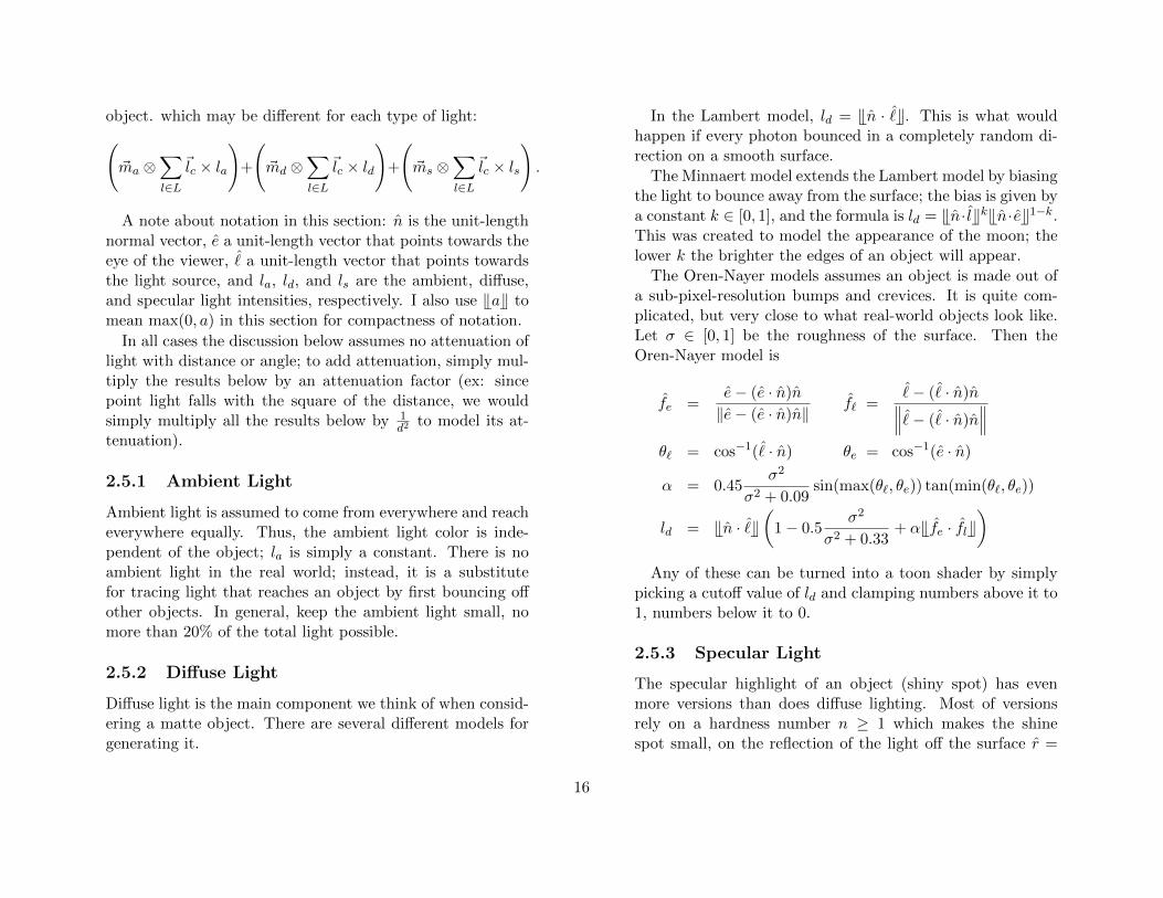
The Oren-Nayer models assumes an object is made out ofa sub-pixel-resolution bumps and crevices. It is quite com-plicated, but very close to what real-world objects look like.Let σ ∈ [0, 1] be the roughness of the surface. Then theOren-Nayer model is

fe =e− (e · n)n‖e− (e · n)n‖

f` =ˆ− (ˆ· n)n∥∥∥ˆ− (ˆ· n)n

∥∥∥θ` = cos−1(ˆ· n) θe = cos−1(e · n)

α = 0.45σ2

σ2 + 0.09sin(max(θ`, θe)) tan(min(θ`, θe))

ld = Tn · ˆU(1− 0.5

σ2

σ2 + 0.33+ αTfe · flU

)Any of these can be turned into a toon shader by simply

picking a cutoff value of ld and clamping numbers above it to1, numbers below it to 0.

2.5.3 Specular Light

The specular highlight of an object (shiny spot) has evenmore versions than does diffuse lighting. Most of versionsrely on a hardness number n ≥ 1 which makes the shinespot small, on the reflection of the light off the surface r =

16

2(n · ˆ)n− ˆ, and/or on the vector halfway between the light

and the eye h =ˆ+e∥∥∥ˆ+e

∥∥∥ .The Phong model is ls = Tr · eUn and the Blinn-Phong

is ls = Th · nUn. They are similar in look and are easy tocompute; generally Blinn-Phong is used in conjunction witha single approximate e and ˆwhile Phong is used if ˆ and/ore vary across the scene.

The Gaussian model is more accurate, but likewise more

expensive to compute: ls = e−m cos−2Tn·hU (note e is Euler’snumber, e is the vector to the eye). Better and more expen-sive is the Beckmann distribution

ls =m

Tn · hU4e−m tan2(cos−1Tn·hU).

Fresnel’s law specifies how much light penetrates a trans-parent object; this can be combined with the Beckmann dis-tribution to get the Cook-Torrance model. Let λ be the Fres-nel factor and β the computed Beckmann distribution; thenCook-Torrance gives

ls = β(1 + Te · nU)λ

Te · nUmin

1,2(h · n

)2 (e · n)

e · h,2(h · n

)2(ˆ· n

)e · h

.

There are also a variety of anisotropic models (notablyHeidrich-Seidel and Ward) which depend additionally uponthe principle tangent vector of the surface and can give theappearance of brushed metal, hair, and the like, but whichare beyond the scope of this booklet.

2.6 Secondary Rays

Shadows, reflection, and transparency are easily achieved us-ing secondary rays: Once you find an intersection point p youthen generate a new ray with p as its origin and intersect thatray with the scene. Care should be taken that roundoff errorsin storing p do not cause the the secondary ray to intersectthe object from which it originates.

2.6.1 Shadows

A point is in shadow relative to a particular light source ifthe ray (p, ˆ) intersects anything closer than the light sourceitself.

2.6.2 Reflection

A mirrored object’s color is given by the ray tracing result ofthe ray (p, 2(n · e)n− e)). A partially mirrored object mixesthat color result with a standard lighting computation at p.One reflection ray might generate another; a cutoff numberof recursions is necessary to prevent infinite loops.

2.6.3 Transparency

Transparency is somewhat more complicated, relying onSnell’s Law. For it to make sense, every surface needs tobe a boundary between two materials, which is not triviallytrue in the case of triangles nor intersecting spheres. How-ever, assuming that we know that the ray is traveling froma material with index of refraction n1 for index of refractionn2, we can derive a rule for finding the transmitted ray.

The cosine of the entering ray is (e · n), meaning that it’ssine is

√1− (e · n)2, or ‖− e−(e · n)n‖2. The sine of the out-

17

going vector thus needs to be n1n2

√1− (e · n); if that is greater

than 1, we have total internal refraction and use the reflec-tion equation instead; otherwise, the cosine of the outgoing

ray is√1− (n1

n2)2(1− (e · n)). Putting this all together, we

have

1: a ⇐ e · n2: b ⇐ n1

n2

√1− (e · n)

3: if b ≥ 1 then4: return 2(n · e)n− e)

5: c ⇐√1− n2

1

n22(1− (e · n))

6: return n1n2(−e− (e · n)n)− cn

2.6.4 Global Illumination

The standard lighting models pretend like the world is di-vided into a small number of light emitters and a vast supplyof things that emit no light. This is obviously not true; ifnothing but light sources gave off photons, we could only seethe light sources themselves. With global illumination, youtry to discover the impact of light bouncing off of the wall,floor, and other objects by creating a number of secondaryrays sampling the diffuse reflection of each object. Ideally, thedistribution of rays should parallel the chosen model of diffuselighting (see Section 2.5.2) and should be so dense as to beintractable for any reasonable scene. Much of the research inphoto-realistic rendering is devoted to finding shortcuts andtechniques that make this process require fewer rays for thesame visual image quality.

2.7 Photon Mapping and Caustics

Photon mapping is raytracing run backwards: instead ofshooting rays from the eye, you shoot them from the lights.The quantity of light reaching each point in the scene isrecorded and used when the scene is rendered, either by ray-tracing or rasterizing. Since many photons leaving a lightsource never reach the eye, this is an inefficient way of cre-ating a single picture; however, it allows lens and mirror-bounced light (called caustics) to be rendered, and it can bemore efficient than viewer-centric global illumination if manyimages are to be made of the same static scene.

2.8 Sub-, Super-, andImportance-Sampling

Sub-sampling is shooting fewer rays than you have pixels, in-terpolating the colors to neighboring pixels. Super-samplingis shooting several rays per pixel, averaging colors to createan anti-aliased image. Importance sampling shoots fewer raysper pixel into “boring” areas and more into “important” ar-eas. Image-space importance sampling shoots more rays intoareas of the scene where neighboring pixels differ in color;scene-space importance sampling shoots more rays towardparticular items.

18