Embed Size (px)
Citation preview

Computer-Controlled SystemsThird Edition
Solutions Manual
Karl J. Åström
Björn Wittenmark
Department of Automatic ControlLund Institute of Technology
October 1997

Preface
This Solutions Manual contains solutions to most of the problems in the fourthedition of
Åström, K. J. and B. Wittenmark (1997): Computer controlled Systems –Theory and Applications, Prentice Hall Inc., Englewood Cliffs, N. J.
Many of the problems are intentionally made such that the students have touse a simulation program to verify the analytical solutions. This is importantsince it gives a feeling for the relation between the pulse transfer function andthe time domain. In the book and the solutions we have used Matlab/Simulink.Information about macros used to generate the illustrations can be obtained bywriting to us.It is also important that a course in digital control includes laboratory exercises.The contents in the laboratory experiments are of course dependent on the avail-able equipment. Examples of experiments are
P Illustration of aliasing
P Comparison between continuous time and discrete time controllers
P State feedback control. Redesign of continuous time controllers as well ascontrollers based on discrete time synthesis
P Controllers based on input-output design
P Control of systems subject to stochastic disturbances.
Finally we would like to thank collegues and students who have helped us to testthe book and the solutions.
Karl J. ÅströmBjörn Wittenmark
Department of Automatic ControlLund Institute of TechnologyBox 118S-220 00 Lund, Sweden
i
Solutions to Chapter 2
Problem 2.1
The system is described byx −ax+ bu
y cx
Sampling the system using (2.4) and (2.5) gives
x(kh+ h) e−ahx(kh) +(
1 − e−ah)(b
a
)u(kh)
y(kh) cx(kh)The pole of the sampled system is exp(−ah). The pole is real. For small valuesof h the pole is close to 1. If a > 0 then the pole moves towards the origin whenh increases. If a < 0 then the pole moves along the positive real axis.
Problem 2.2
a. Using the Laplace transform method we find that
Φ eAh L−1((
sI − A)−1)
L−1
(1
s2 + 1
s 1
−1 s
) cos h sin h
− sin h cos h
Γ
h∫0
eAsB ds h∫
0
sin s
cos s
ds 1− cos h
sin h
b. The system has the transfer function
G(s) s+ 3s2 + 3s+ 2
s+ 3(s+ 1)(s+ 2)
2s+ 1
− 1s+ 2
Using the Table 2.1 gives
H(q) 21 − e−h
q− e−h −1− e−2h
2(
q− e−2h)
c. One state space realization of the system is
x
0 0 0
1 0 0
0 1 0
x+
1
0
0
u
y 0 0 1
x
Now
A2
0 0 0
0 0 0
1 0 0
A3 0
1
then
eAh I + Ah+ A2h2/2+ ( ( (
1 0 0
h 1 0
h2/2 h 1
Γ
h∫0
eAsB ds h∫
0
1 s s2/2T
ds h h2/2 h3/6
T
and
H(q) C(qI − Φ)−1Γ
0 0 1
(q− 1)3x x x
x x x
h2(q+ 1)/2 h(q− 1) (q− 1)2
h
h2/2h3/6
h3(q2 + 4q+ 1)
6(q− 1)3
Problem 2.3
Φ eAh ⇒ A 1h
ln Φ
a.y(k)− 0.5y(k− 1) 6u(k− 1)
y− 0.5q−1y 6q−1u
qy− 0.5y 6ux(kh+ h) 0.5x(kh)+ 6u(kh)y(kh) x(kh)
x(t) ax(t) + bu(t)y(t) x(t)
(discrete-time system) (continuous time system)Φ eah 0.5
Γ h∫
0easb ds 6
ah ln 0.5 ⇒ a − ln 2h
h∫0
eas b ds ba
eas
∣∣∣∣h0 b
a
(eah − 1
) 6
⇒ b 6aeah − 1
12 ln2h
b. x(kh+ h)
−0.5 1
0 −0.3
x(kh) + 0.5
0.7
u(kh)
y(kh) 1 1
x(kh)Eigenvalue to Φ:
det(sI − Φ) s+ 0.5 −1
0 s+ 0.3
0 ⇔ (s+ 0.5)(s+ 0.3) 0
λ 1 −0.5 λ 2 −0.3
Both eigenvalues of Φ on the negative real axis ⇒ No corresponding contin-uous system exists.
2
c.y(k) + 0.5y(k− 1) 6u(k− 1) ⇔y(k+ 1) −0.5y(k)+ 6u(t)H(q) 6
q+ 0.5one pole on the negative real axis.
⇒ No equivalent continuous system exists.
Problem 2.4
Harmonic oscillator (cf. A.3 and 3.2a).x(k+ 1) Φx(k) + Γu(k)y(k) C x(k) Φ(h)
cos h sin h
− sin h cos h
Γ(h)
1− cos h
sin h
a.
h π2
⇒ Φ 0 1
−1 0
Γ 1
1
y
1 0 x
Pulse transfer operator
H(q) C(qI − Φ)−1Γ 1 0
q −1
1 q
−1 1
1
1
q2 + 1
1 0 q 1
−1 q
1
1
q+ 1q2 + 1
Y(z) H(z)U(z) z+ 1z2 + 1
⋅z
z− 1 1
z2 + 1+ 1
z− 1
y(k) sinπ2(k− 1)θ (k− 1) + θ (k− 1)
(1 − cos
π2
k)
θ (k− 1)where θ (k− 1) is a step at k 1.
G(s) [see Probl. 2.2] 1 0
s −1
1 s
−1 0
1
1s2 + 1
Y(s) 1s(s2 + 1)
1s− s
s2 + 1
y(t) 1− cos t
y(kh) 1− cosπ2
k
b. The same way as a. ⇒ y(t) 1− cos t, and y(kh) 1− cos π4 k Notice that
the step responses of the continuous time and the zero-order hold sampledsystems are the same in the sampling points.
Problem 2.5
Do a partial fraction decomposition and sample each term using Table 2.1:
G(s) 1s2(s+ 2)(s+ 3)
16
1s2 −
536
1s+ 1
41
s+ 2− 1
91
s+ 3
H(q) 112
q+ 1(q− 1)2 −
536
1q− 1
+ 18
1 − e−2
q− e−2 −1
271− e−3
q − e−3
3
Problem 2.6
Integrating the system equation
x Ax + Bu
gives
x(kh+ h) eAhx(kh) +kh+h∫kh
eAsBδ (s − kh)u(kh)ds
eAhx(kh) + Bu(kh)
Problem 2.7
The representation (2.7) is
x(kh+ h) Φx(kh) + Γu(kh)y(kh) C x(kh)
and the controllable form realization is
z(kh+ h) Φz(kh)+ Γu(kh)y(kh) C z(kh)
where
Φ 1 h
0 1
Γ h2/2
h
Φ 2 −1
1 0
Γ 1
0
C
1 0 C
h2/2 h2/2
From Section 2.5 we get
Φ TΦT−1 or ΦT TΦ
Γ TΓ
C CT−1 or C T C
This gives the following relations
t11 2t11 − t21
t21 t11 (1)ht11 + t12 2t12 − t22 (2)ht21 + t22 t12
h2
2t11 + ht12 1
h2
2t21 + ht22 0
h2
2t11 + h2
2t21 1 (3)
h2
2t12 + h2
2t22 0 (4)
Equations (1)–(4) now give
t11 t21 1/h2
t12 −t22 1/(2h) or T 12h2
2 h
2 −h
4
Problem 2.8
The pulse transfer function is given by
H(z) C(zI − Φ)−1Γ
1 0
z(z− 0.5) z − 0.2
0 z− 0.5
2
1
2z− 0.2
z(z− 0.5) 2(z− 0.1)z(z− 0.5)
Problem 2.9
The system is described by
x −a b
c −d
x+ f
g
u Ax + Bu
The eigenvalues of A is obtained from
(λ + a)(λ + d)− bc λ 2 + (a+ d)λ + ad− bc 0
which gives
λ −a+ d2
±
√(a− d)2 + 4bc
4The condition that aA bA c, and d are nonnegative implies that the eigenvalues, λ 1
and λ 2, are real. There are multiple eigenvalues if both a d and bc 0. Usingthe result in Appendix B we find that
eAh α 0I +α 1 Ah
andeλ1h α 0 +α 1λ 1h
eλ2h α 0 +α 1λ 2h
This gives
α 0 λ 1eλ2h − λ 2eλ1h
λ 1 − λ 2
α 1 eλ1h − eλ2h
(λ 1 − λ 2)h
Φ α 0 −α 1ah α 1bh
α 1ch α 0 −α 1dh
To compute Γ we notice that α 0 and α 1 depend on h. Introduce
β 0 h∫
0
α 0(s)ds 1λ 1 − λ 2
(λ 1
λ 2
(eλ2h − 1
)− λ 2
λ 1
(eλ1h − 1
))
β 1 h∫
0
sα 1(s)ds 1λ 1 − λ 2
(1
λ 1
(eλ1h − 1
)− 1
λ 2
(eλ2h − 1
))
thenΓ β 0 B + β 1 AB
5
Problem 2.10
a. Using the result from Problem 2.9 gives
λ 1 −0.0197 eλ1h 0.7895
λ 2 −0.0129 eλ2h 0.8566
Further
α 0 0.9839 α 1 0.8223
and
Φ α 0I + 12α 1A 0.790 0
0.176 0.857
β 0 11.9412
β 1 63.3824
Γ (β 0 I + β 1 A) B 0.281
0.0296
b. The pulse transfer operator is now given by
H(q)C(qI − Φ)−1Γ 0 1
q − 0.790 0
−0.176 q − 0.857
−1 0.281
0.0297
0.030q+ 0.026
q2 − 1.65q+ 0.68
which agrees with the pulse transfer operator given in the problem formula-tion.
Problem 2.11
The motor has the transfer function G(s) 1/(s(s+ 1)). A state space represen-tation is given in Example A.2, where
A −1 0
1 0
B 1
0
C 0 1
Φ exp(Ah) L−1
((sI − A)−1
) L−1
(1
s(s+ 1) s 0
1 s+ 1
) e−h 0
1 − e−h 1
Γ
h∫0
eAsBds h∫
0
e−s
1 − e−s
ds 1− e−h
h+ e−h − 1
This gives the sampled representation given in Example A.2.
6
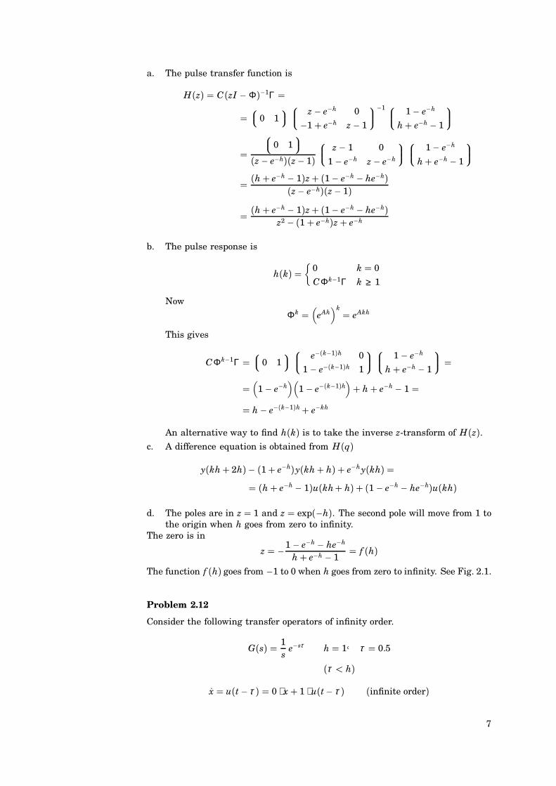
a. The pulse transfer function is
H(z) C(zI − Φ)−1Γ
0 1
z− e−h 0
−1+ e−h z− 1
−1 1− e−h
h+ e−h − 1
0 1
(z− e−h)(z− 1) z− 1 0
1 − e−h z− e−h
1− e−h
h+ e−h − 1
(h+ e−h − 1)z+ (1− e−h − he−h)
(z− e−h)(z− 1)
(h+ e−h − 1)z+ (1− e−h − he−h)z2 − (1+ e−h)z+ e−h
b. The pulse response is
h(k)
0 k 0
CΦk−1Γ k ≥ 1
Now
Φk (
eAh)k eAkh
This gives
CΦk−1Γ 0 1
e−(k−1)h 0
1 − e−(k−1)h 1
1 − e−h
h+ e−h − 1
(
1 − e−h)(
1 − e−(k−1)h)+ h+ e−h − 1
h− e−(k−1)h+ e−kh
An alternative way to find h(k) is to take the inverse z-transform of H(z).c. A difference equation is obtained from H(q)
y(kh+ 2h)− (1+ e−h)y(kh+ h) + e−hy(kh) (h+ e−h − 1)u(kh+ h) + (1 − e−h − he−h)u(kh)
d. The poles are in z 1 and z exp(−h). The second pole will move from 1 tothe origin when h goes from zero to infinity.
The zero is in
z −1 − e−h − he−h
h+ e−h − 1 f (h)
The function f (h) goes from −1 to 0 when h goes from zero to infinity. See Fig. 2.1.
Problem 2.12
Consider the following transfer operators of infinity order.
G(s) 1s
e−sτ h 1A τ 0.5
(τ < h)
x u(t− τ ) 0 ⋅ x+ 1 ⋅ u(t− τ ) (infinite order)
7
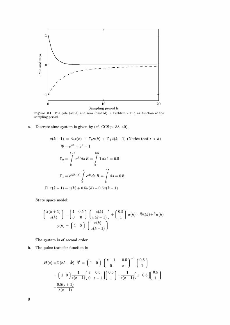
0 10 20
−1
0
1P
ole
and
zero
Sampling period hFigure 2.1 The pole (solid) and zero (dashed) in Problem 2.11.d as function of thesampling period.
a. Discrete time system is given by (cf. CCS p. 38–40).
x(k+ 1) Φx(k) + Γ0u(k) + Γ1u(k− 1) (Notice that τ < h)Φ eAh e0 1
Γ0 h−τ∫0
eAsds B 0.5∫0
1 ds 1 0.5
Γ1 eA(h−τ )τ∫
0
eAsds B 0.5∫0
ds 0.5
⇒ x(k+ 1) x(k) + 0.5u(k)+ 0.5u(k− 1)
State space model:
x(k+ 1)u(k)
1 0.50 0
x(k)u(k− 1)
+ 0.51
u(k) Φx(k)+Γu(k)
y(k) 1 0
x(k)u(k− 1)
The system is of second order.
b. The pulse-transfer function is
H(z) C(zI − Φ)−1Γ 1 0
z− 1 −0.50 z
−1 0.51
1 0
1z(z− 1)
z 0.50 z− 1
0.51
1z(z− 1)
z 0.50.5
1
0.5(z+ 1)
z(z− 1)
8
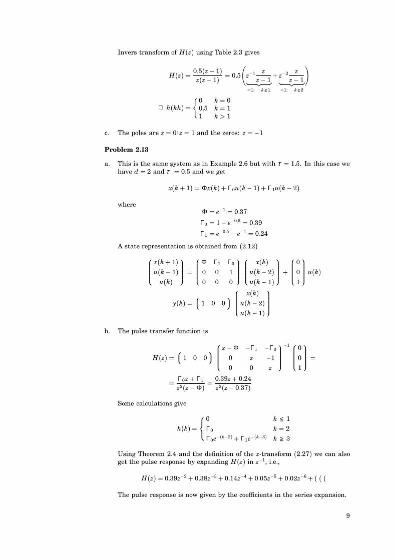
Invers transform of H(z) using Table 2.3 gives
H(z) 0.5(z+ 1)z(z− 1) 0.5
(z−1 z
z− 1︸ ︷︷ ︸1; k ≥ 1
+ z−2 zz− 1︸ ︷︷ ︸
1; k ≥ 2
)
⇒ h(kh)
0 k 00.5 k 11 k > 1
c. The poles are z 0A z 1 and the zeros: z −1
Problem 2.13
a. This is the same system as in Example 2.6 but with τ 1.5. In this case wehave d 2 and τ ′ 0.5 and we get
x(k+ 1) Φx(k)+ Γ0u(k− 1) + Γ1u(k− 2)
whereΦ e−1 0.37
Γ0 1 − e−0.5 0.39
Γ1 e−0.5 − e−1 0.24
A state representation is obtained from (2.12)x(k+ 1)u(k− 1)
u(k)
Φ Γ1 Γ0
0 0 1
0 0 0
x(k)u(k− 2)u(k− 1)
+
0
0
1
u(k)
y(k) 1 0 0
x(k)u(k− 2)u(k− 1)
b. The pulse transfer function is
H(z) 1 0 0
z− Φ −Γ1 −Γ0
0 z −1
0 0 z
−1
0
0
1
Γ0z+ Γ1
z2(z− Φ) 0.39z+ 0.24z2(z− 0.37)
Some calculations give
h(k)
0 k ≤ 1
Γ0 k 2
Γ0e−(k−2) + Γ1e−(k−3) k ≥ 3
Using Theorem 2.4 and the definition of the z-transform (2.27) we can alsoget the pulse response by expanding H(z) in z−1, i.e.,
H(z) 0.39z−2+ 0.38z−3+ 0.14z−4+ 0.05z−5+ 0.02z−6+ ( ( (
The pulse response is now given by the coefficients in the series expansion.
9
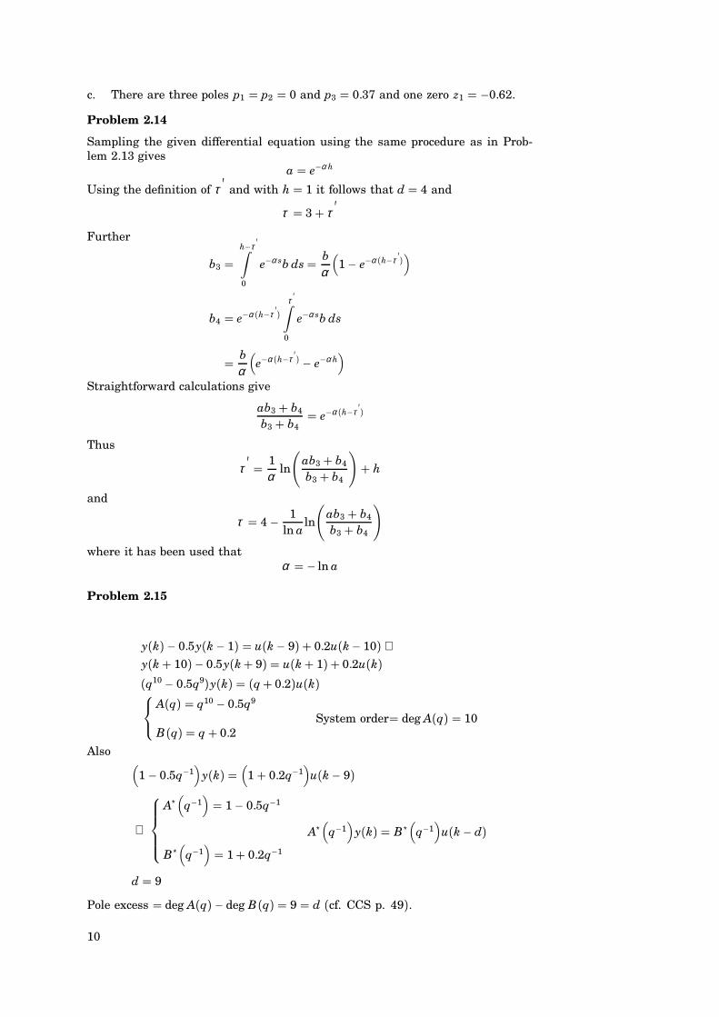
c. There are three poles p1 p2 0 and p3 0.37 and one zero z1 −0.62.
Problem 2.14
Sampling the given differential equation using the same procedure as in Prob-lem 2.13 gives
a e−α h
Using the definition of τ ′ and with h 1 it follows that d 4 and
τ 3+ τ ′
Further
b3 h−τ ′∫0
e−α sb ds bα
(1− e−α (h−τ ′)
)
b4 e−α (h−τ ′)τ ′∫
0
e−α sb ds
bα
(e−α (h−τ ′) − e−α h
)Straightforward calculations give
ab3 + b4
b3 + b4 e−α (h−τ ′)
Thus
τ ′ 1α ln
(ab3 + b4
b3 + b4
)+ h
and
τ 4 − 1ln a
ln
(ab3 + b4
b3 + b4
)where it has been used that
α − ln a
Problem 2.15
y(k)− 0.5y(k− 1) u(k− 9) + 0.2u(k− 10)⇔y(k+ 10)− 0.5y(k+ 9) u(k+ 1) + 0.2u(k)(q10 − 0.5q9)y(k) (q+ 0.2)u(k) A(q) q10 − 0.5q9
System order deg A(q) 10B(q) q+ 0.2
Also (1 − 0.5q−1
)y(k)
(1+ 0.2q−1
)u(k− 9)
⇒
A∗(
q−1) 1− 0.5q−1
A∗(
q−1)
y(k) B∗(
q−1)
u(k− d)B∗(
q−1) 1+ 0.2q−1
d 9
Pole excess deg A(q)− deg B(q) 9 d (cf. CCS p. 49).
10
Remark
B(q)A(q)
q+ 0.2q10 − 0.5q9
q−10(q+ 0.2)q−10
(q10 − 0.5q1
) q−9+ 0.2q−10
1 − 0.5q−1
q−9
(1+ 0.2q−1
)(
1 − 0.5q−1) q−d
B∗(
q−1)
A∗(
q−1)
Problem 2.16
FIR filter:
H∗(
q−1) b0 + b1q−1 + ( ( (+ bnq−n
y(k) (
b0 + b1q−1 + ( ( ( + bnq−n)
u(k) b0u(k)+ b1u(k− 1) + ( ( ( + bnu(k− n)
⇒ y(k+ n) b0u(k+ n) + b1u(k+ n− 1) + ( ( ( + bnu(k)
⇒ qny(k) (
b0qn + b1qn−1 + ( ( ( + bn
)u(k)
⇒ H(q) b0qn + b1qn−1 + ( ( ( + bn
qn b0 + b1qn−1+ ( ( (+ bn
qn
n:th order system
H(q) D + B(q)A(q)
b. Observable canonical form:
Φ
−a1 1 0 ( ( ( 0
−a2 0 1 ( ( ( 0
1
−an 0 0
0 1 0 ( ( ( 0
0 0 1 0
1
0 0
Γ
b1
...
bn
C
1 0 ( ( ( 0 D b0
Problem 2.17
y(k+ 2)− 1.5y(k+ 1) + 0.5y(k) u(k+ 1) ⇔
q2 y(k)− 1.5qy(k)+ 0.5y(k) qu(k)Use the z-transform to find the output sequence when
u(k)
0 k < 0
1 k ≥ 0
y(0) 0.5y(−1) 1
Table 2.2 (page 57):
Z(
qn f) zn
(F − F1
); F1(z)
n−1∑j0
f (jh)z−j
⇒ z2(
Y − y(0)− y(1)z−1)− 1.5z
(Y − y(0)
)+ 0.5Y z
(U − u(0)
)11
Compute
y(1) u(0)− 0.5y(−1) + 1.5y(0) 1− 0.5+ 0.75 1.25
⇒ z2(
Y − 0.5− 1.25z−1)− 1.5z(Y − 0.5) + 0.5Y z(U − 1)(
z2 − 1.5z+ 0.5)
Y − 0.5z2 − 1.25z+ 0.75z zU − z
Y(z) 0.5z2 − 0.5zz2 − 1.5z+ 0.5
+ zz2 − 1.5z+ 0.5
U(z)
0.5z(z− 1)(z− 1)(z− 0.5) +
z(z− 1)(z− 0.5) U(z)
U zz− 1
(step) ⇒
Y(z) 0.5zz− 0.5
+ z2
(z− 1)2(z− 0.5) 0.5z
z− 0.5+ 2(z− 1)2 +
1z− 0.5
Table 2.3 (page 59) gives via inverse transformation.
Z−1(
zz− e−1/T
) e−k/T ; e−1/T 0.5 ⇒ T 1
ln 2
Z−1(
z−1 zz− 0.5
) e−(k−1)⋅ln2
Z−1(
1(z− 1)2
)Z−1
(z−1 z(z− 1)2
) k− 1 (h 1)
⇒ y(k) 0.5e−k⋅ln2 + 2(k− 1) + e−(k−1) ln2
y(1) 1.25
y(0) 0.5
y(−1) 1
Checking the result:
y(2) 0.5e−2 ln2 + 2+ e− ln2 18+ 2+ 1
2 21
8
y(2) u(1) + 1.5y(1)− 0.5y(0) 1+ 1.5 ⋅ 1.25− 0.52
1+ 32
⋅54− 1
4 21
8
12
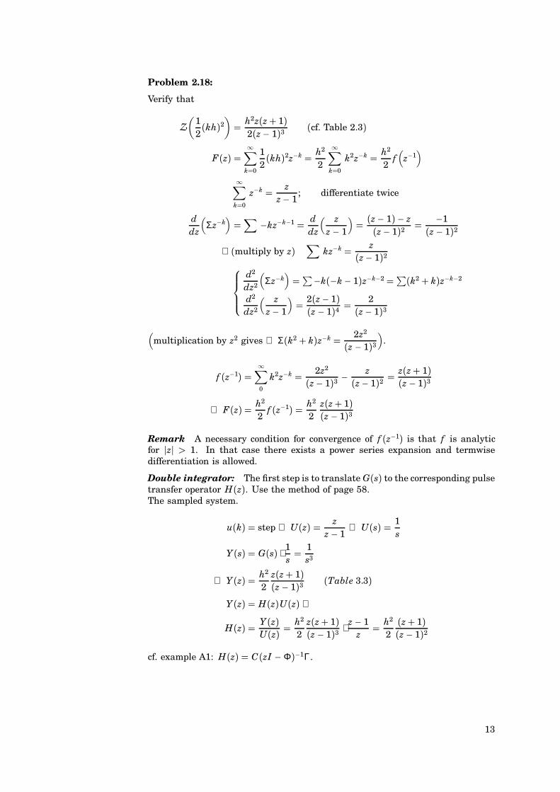
Problem 2.18:
Verify that
Z(
12(kh)2
) h2z(z+ 1)
2(z− 1)3 (cf. Table 2.3)
F(z) ∞∑
k0
12(kh)2z−k h2
2
∞∑k0
k2z−k h2
2f(
z−1)
∞∑k0
z−k zz− 1
; differentiate twice
ddz
(Σz−k
)∑
−kz−k−1 ddz
( zz− 1
) (z− 1)− z
(z− 1)2 −1(z− 1)2
⇒(multiply by z)∑
kz−k z(z− 1)2
d2
dz2
(Σz−k
)∑−k(−k− 1)z−k−2 ∑(k2 + k)z−k−2
d2
dz2
( zz− 1
) 2(z− 1)(z− 1)4
2(z− 1)3
(multiplication by z2 gives ⇒ Σ(k2 + k)z−k 2z2
(z− 1)3)
.
f (z−1) ∞∑0
k2z−k 2z2
(z− 1)3 −z
(z− 1)2 z(z+ 1)(z− 1)3
⇒ F(z) h2
2f (z−1) h2
2z(z+ 1)(z− 1)3
Remark A necessary condition for convergence of f (z−1) is that f is analyticfor jzj > 1. In that case there exists a power series expansion and termwisedifferentiation is allowed.
Double integrator: The first step is to translate G(s) to the corresponding pulsetransfer operator H(z). Use the method of page 58.The sampled system.
u(k) step ⇒ U(z) zz− 1
⇒ U(s) 1s
Y(s) G(s) ⋅1s 1
s3
⇒ Y(z) h2
2z(z+ 1)(z− 1)3 (Table 3.3)
Y(z) H(z)U(z)⇒
H(z) Y(z)U(z)
h2
2z(z+ 1)(z− 1)3 ⋅
z− 1z
h2
2(z+ 1)(z− 1)2
cf. example A1: H(z) C(zI − Φ)−1Γ.
13

Problem 2.19
a. The transfer function of the continuous time system is
G(s) bc(s+ a)
Equation (2.30) gives
H(z) 1z− e−ah Ress−a
(esh − 1
sbc
s+ a
) 1
z− e−ah
e−ah − 1−a
bc
bca
1− e−ah
z− e−ah
This is the same result as obtained by using Table 2.1.
b. The normalized motor has the transfer function
G(s) 1s(s+ 1)
and we get
H(z) ∑ssi
1z− esh Res
(esh − 1
s1
s(s+ 1))
To compute the residue for s 0 we can use the series expansion of (esh−1)/sand get
H(z) 1z− e−h
e−h − 1(−1)2 + h
z− 1
(z− 1)(e−h− 1) + h(z− e−h)(z− e−h)(z− 1)
(e−h − 1+ h)z+ (1− e−h − he−h)
(z− e−h)(z− 1)Compare Problem 2.11.
Problem 2.21s+ βs+α
is lead if β < α
Consider the discrete time system
z+ bz+ a
arg(
eiω h + beiω h + a
) arg
(cosωh+ b+ i sinωhcosωh + a+ i sinωh
)
arctan(
sinωhb+ cosωh
)− arctan
(sinωh
a+ cosωh
)Phase lead if
arctan(
sinωhb+ cosωh
)> arctan
sinωha+ cosωh
0 < ωh < π
sinωhb+ cosωh
> sinωha+ cosωh
We thus get phase lead if b < a.
14
0 10 200
10
Ou
tpu
t
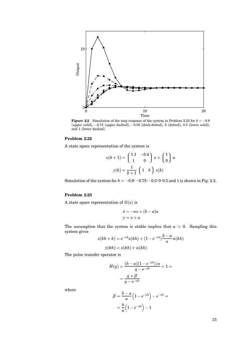
TimeFigure 2.2 Simulation of the step response of the system in Problem 2.22 for b −0.9(upper solid), −0.75 (upper dashed), −0.50 (dash-dotted), 0 (dotted), 0.5 (lower solid),and 1 (lower dashed).
Problem 2.22
A state space representation of the system is
x(k+ 1) 1.1 −0.4
1 0
x+ 1
0
u
y(k) 1b+ 1
1 b x(k)
Simulation of the system for b −0.9A−0.75A−0.5A0A0.5 and 1 is shown in Fig. 2.2.
Problem 2.23
A state space representation of G(s) is
x −ax + (b− a)uy x+ u
The assumption that the system is stable implies that a > 0. Sampling thissystem gives
x(kh+ h) e−ahx(kh) + (1− e−ah)b− aa
u(kh)
y(kh) x(kh)+ u(kh)The pulse transfer operator is
H(q) (b− a)(1− e−ah)/aq− e−ah + 1
q+ βq − e−ah
where
β b− aa
(1− e−ah
)− e−ah
ba
(1− e−ah
)− 1
15

The inverse is stable if ∣∣∣∣ba(1 − e−ah)− 1∣∣∣∣ < 1
or
0 < ba(1− e−ah) < 2
Since a > 0 and (1− e−ah) > 0 then
0 < b < 2a1 − e−ah
For b > 0 we have the cases
b ≤ 2a The inverse is stable independent of h.
b > 2a Stable inverse if ah < ln(b/(b− 2a)).
Problem 2.28
y(k) y(k− 1) + y(k− 2) y(0) y(1) 1
The equation has the characteristic equation
z2 − z− 1 0
which has the solution
z12 1 ±√
52
The solution has the form
y(k) c1
(1+√5
2
)k
+ c2
(1 −
√5
2
)k
Using the initial values give
c1 1
2√
5(√
5+ 1)
c2 1
2√
5(√
5− 1)
Problem 2.29
The system is given by(1 − 0.5q−1+ q−2) y(k) (2q−10+ q−11)u(k)
Multiply by q11. This gives
q9 (q2 − 0.5q+ 1)
y(k) (2q+ 1)u(k)
The system is of order 11 ( deg A(q)) and has the poles
p12 1 ± i√
154
p3...11 0 (multiplicity 9)
and the zeroz1 −0.5
16
Problem 2.30
The system H1 has a pole on the positive real axis and can be obtained by samplinga system with the transfer function
G(s) Ks+ a
H2 has a single pole on the negative real axis and has no continuous time equiv-alent.The only way to get two poles on the negative real axis as in H3 is when thecontinuous time system have complex conjugate poles given by
s2 + 2ζ ω0s+ω20 0
Further we must sample such that h π/ω where
ω ω0
√1 − ζ 2
We have two possible cases
G1(s) ω20
s2 + 2ζ ω0s+ω20
i)
G2(s) ss2 + 2ζ ω0s+ω2
0ii)
Sampling G1 with h π/ω gives, (see Table 2.1)
H(z) (1+α )(q+α )(q+α )2 1+α
q+α
whereα e−ζ ω0h
i.e., we get a pole zero concellation. Sampling G2 gives H(z) 0. This impliesthat H3 cannot be obtained by sampling a continuous time system. H4 can berewritten as
H4(q) 2+ 0.9q− 0.8q(q− 0.8)
The second part can be obtained by sampling a first order system with a timedelay. Compare Example 2.8.
Problem 2.31
We can rewrite G(s) as
G(s) 1s+ 1
+ 1s+ 3
Using Table 2.1 gives
H(q) 1 − e−h
q − e−h +13
⋅1− e−3h
q − e−3h
With h 0.02 we get
H(q) 0.0392q− 0.0377(q− 0.9802)(q− 0.9418)
17
Problem 2.32
x 1 0
1 1
x+ 1
0
u(t− τ ) τ 0.2 h 0.3
Φ L−1(sI − A
)−1 L−1
s− 1 0
−1 s− 1
−1
L−1
1
s− 10
1(s− 1)2
1s− 1
eh 0
heh eh
Γ0 h−τ∫0
es
ses
ds es
ses
h−τ
0
−h−τ∫0
0
es
ds
eh−τ − 1
(h− τ )eh−τ − eh−τ + 1
−1+ eh−τ
1+ (h− τ − 1)eh−τ
Γ1 eA(h−τ )
τ∫0
e−s
se−s
ds eh−τ 0
(h− τ )eh−τ eh−τ
−1+ eτ
1+ (τ − 1)eτ
eh−τ (−1+ eτ )
eh−τ (1 − h+ τ ) + (h− 1)eh
The pulse transfer operator is given by
H(q) C(qI − Φ)−1(Γ0 + Γ1q−1)
where
Φ 1.350 0
0.405 1.350
Γ0 0.105
0.005
Γ1 0.245
0.050
18
Solutions to Chapter 3
Problem 3.1
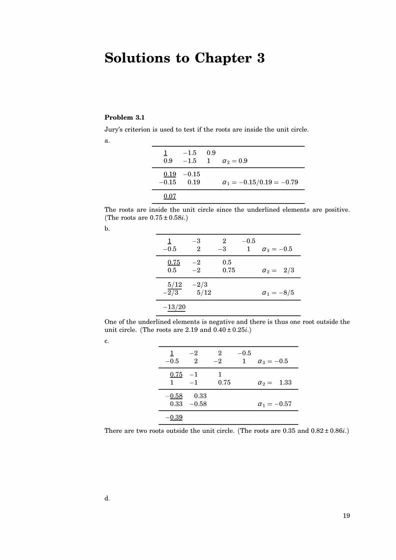
Jury’s criterion is used to test if the roots are inside the unit circle.
a.
1 −1.5 0.90.9 −1.5 1 α 2 0.9
0.19 −0.15−0.15 0.19 α 1 −0.15/0.19 −0.79
0.07
The roots are inside the unit circle since the underlined elements are positive.(The roots are 0.75 ± 0.58i.)b.
1 −3 2 −0.5−0.5 2 −3 1 α 3 −0.5
0.75 −2 0.50.5 −2 0.75 α 2 2/35/12 −2/3
−2/3 5/12 α 1 −8/5−13/20
One of the underlined elements is negative and there is thus one root outside theunit circle. (The roots are 2.19 and 0.40 ± 0.25i.)c.
1 −2 2 −0.5−0.5 2 −2 1 α 3 −0.5
0.75 −1 11 −1 0.75 α 2 1.33
−0.58 0.330.33 −0.58 α 1 −0.57
−0.39
There are two roots outside the unit circle. (The roots are 0.35 and 0.82 ± 0.86i.)
d.
19
1 5 −0.25 −1.25−1.25 −0.25 5 1 α 3 −1.25
−0.56 4.69 66 4.69 −0.56 α 2 −10.71
63.70 54.9254.92 63.70 α 1 0.86
16.47
One root is outside the unit circle. (The roots are −5A−0.5, and 0.5.)e.
1 −1.7 1.7 −0.7−0.7 1.7 −1.7 1 α 3 −0.7
0.51 −0.51 0.510.51 −0.51 0.51 α 2 1
0 00 0
The table breaks down since we can not compute α 1. There is one of the underlinedelements that is zero which indicates that there is at least one root on the stabilityboundary. (The roots are 0.7 and 0.5 ± 0.866i. The complex conjugate roots are onthe unit circle.)
Problem 3.2
The characteristic equation of the closed loop system is
z(z− 0.2)(z− 0.4) + K 0 K > 0
The stability can be determined using root locus. The starting points are z 0A0.2and 0.4. The asymptotes have the directions ±π/3 and −π . The crossing pointof the asymptotes is 0.2. To find where the roots will cross the unit circle letz a+ ib, where a2 + b2 1. Then
(a+ ib)(a+ ib − 0.2)(a+ ib − 0.4) −K
Multiply with a − ib and use a2 + b2 1.
a2 − 0.6a− b2 + 0.08+ i(2ab− 0.6b) −K (a− ib)Equate real and imaginary parts.
a2 − 0.6a− b2 + 0.08 −K a
b(2a− 0.6) K b
If b 6 0 thena2 − 0.6a−
(1 − a2)+ 0.08 −a(2a− 0.6)
4a2 − 1.2a− 0.92 0
The solution is
a12 0.15 ±√
0.0225+ 0.23 0.15 ± 0.502
0.652−0.352
This gives K 2a− 0.6 0.70 and −1.30. The root locus may also cross the unitcircle for b 0, i.e. a ±1. A root at z −1 is obtained when
−1(−1− 0.2)(−1− 0.4) + K 0
20
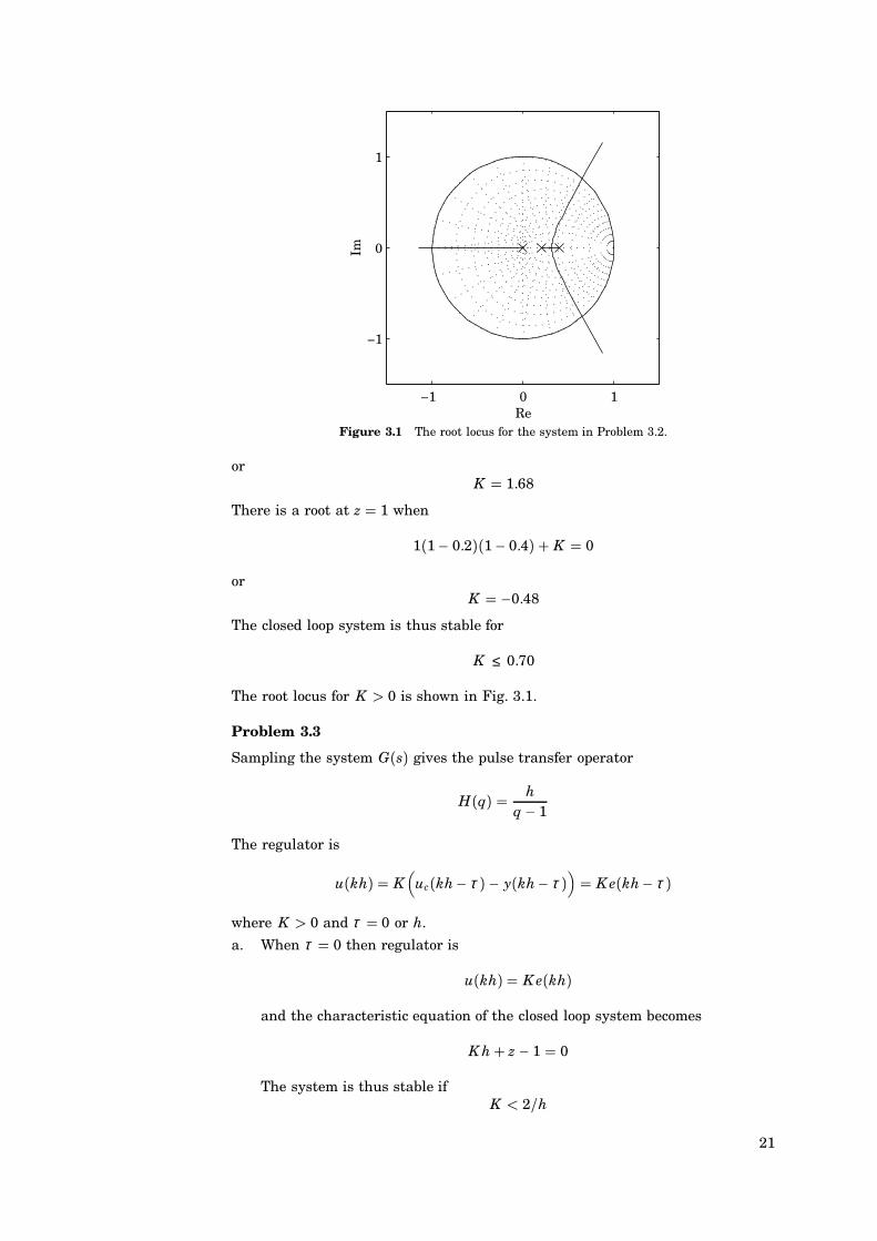
−1 0 1
−1
0
1
Re
Im
Figure 3.1 The root locus for the system in Problem 3.2.
orK 1.68
There is a root at z 1 when
1(1− 0.2)(1− 0.4) + K 0
orK −0.48
The closed loop system is thus stable for
K ≤ 0.70
The root locus for K > 0 is shown in Fig. 3.1.
Problem 3.3
Sampling the system G(s) gives the pulse transfer operator
H(q) hq − 1
The regulator is
u(kh) K(
uc(kh− τ )− y(kh− τ )) K e(kh− τ )
where K > 0 and τ 0 or h.
a. When τ 0 then regulator is
u(kh) K e(kh)
and the characteristic equation of the closed loop system becomes
K h+ z− 1 0
The system is thus stable ifK < 2/h
21
When there is a delay of one sample (τ h) then the regulator is
u(kh) Kq
e(kh)
and the characteristic equation is
K h+ z(z− 1) z2 − z+ K h 0
The constant term is the product of the roots and it will be unity when thepoles are on the unit circle. The system is thus stable if
K < 1/h
b. Consider the continuous system G(s) in series with a time delay of τ seconds.The transfer function for the open loop system is
Go(s) Ks
e−sτ
The phase function isarg Go(iω) −π
2− wτ
and the gain is
jGo(iω)j Kω
The system is stable if the phase lag is less than π at the cross over frequency
jGo(iω c)j 1
⇒ ω c K
The system is thus stable if
−π/2−ω cτ > −π
K < π/2τ
∞ τ 0π2h τ h
The continuous time system will be stable for all values of K if τ 0 andfor K < π/(2h) when τ h. This value is about 50% larger than the valueobtained for the sampled system in b.
Problem 3.4
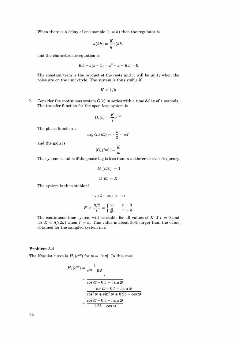
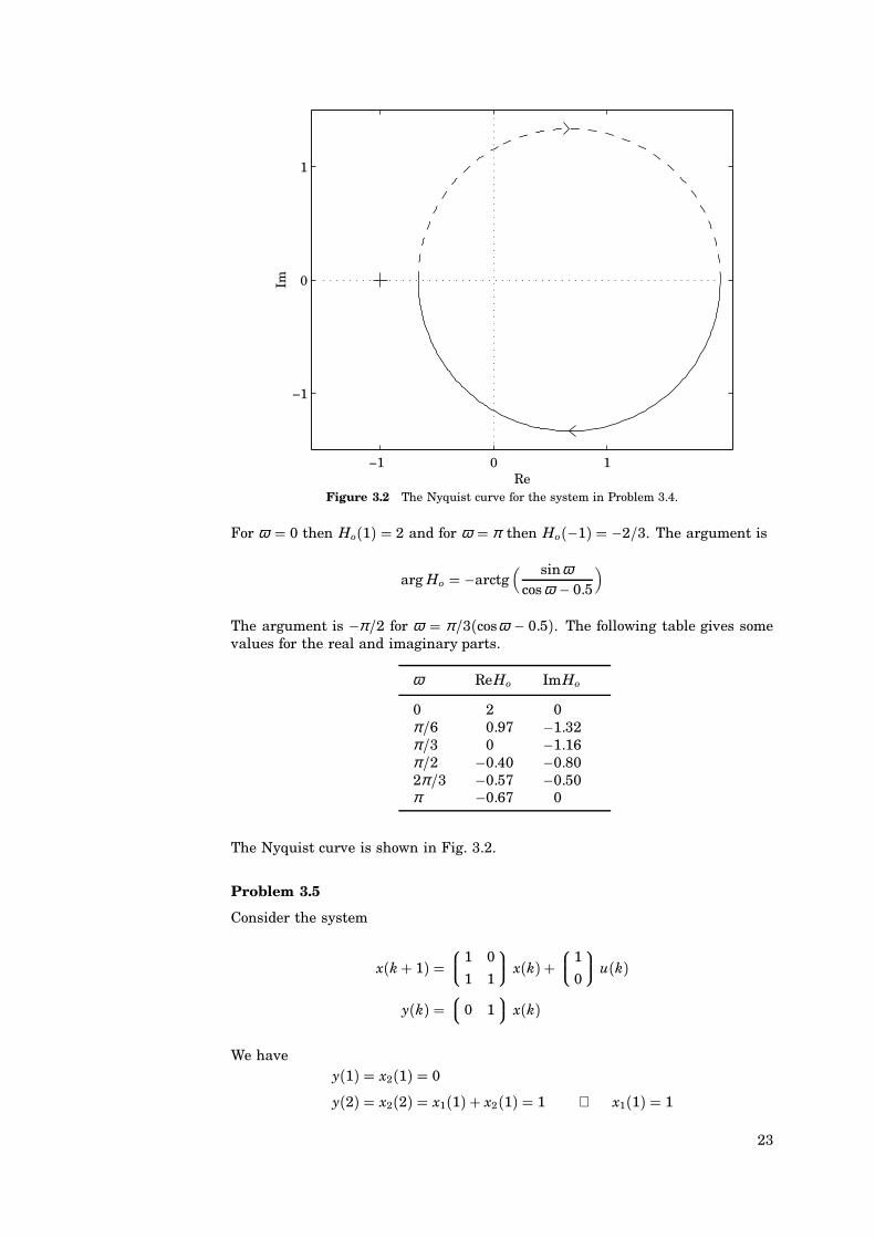
The Nyquist curve is Ho(eiω) for ω [0Aπ ]. In this case
Ho(eiω) 1eiω − 0.5
1cosω − 0.5+ i sinω
cosω − 0.5− i sinωcos2 ω + sin2 ω + 0.25− cosω
cosω − 0.5 − i sinω1.25− cosω
22
−1 0 1
−1
0
1
Re
Im
Figure 3.2 The Nyquist curve for the system in Problem 3.4.
For ω 0 then Ho(1) 2 and for ω π then Ho(−1) −2/3. The argument is
arg Ho −arctg( sinω
cosω − 0.5
)The argument is −π/2 for ω π/3(cosω − 0.5). The following table gives somevalues for the real and imaginary parts.
ω ReHo ImHo
0 2 0π/6 0.97 −1.32π/3 0 −1.16π/2 −0.40 −0.802π/3 −0.57 −0.50π −0.67 0
The Nyquist curve is shown in Fig. 3.2.
Problem 3.5
Consider the system
x(k+ 1) 1 0
1 1
x(k) + 1
0
u(k)
y(k) 0 1
x(k)
We havey(1) x2(1) 0
y(2) x2(2) x1(1) + x2(1) 1 ⇒ x1(1) 1
23
Further
x(2) Φx(1) + Γu(1) 1 0
1 1
1
0
+ 1
0
⋅ 1 2
1
x(3)
1 0
1 1
2
1
+ 1
0
⋅ (−1) 1
3
The possibility to determine x(1) from y(1), y(2) and u(1) is called observability.
Problem 3.6
a. The observability matrix is
Wo C
CΦ
2 −4
1 −2
The system is not observable since det Wo 0.
b. The controllability matrix is
Wc Γ ΦΓ
6 1
4 1
det Wc 2 and the system is reachable.
Problem 3.7
The controllability matrix is
Wc Γ ΦΓ
1 1 1 1
1 0 0.5 0
For instance, the first two colums are linearly independent. This implies that Wc
has rank 2 and the system is thus reachable. From the input u′ we get the system
x(k+ 1) 1 0
0 0.5
x(k) +0
1
u′(k)
In this case
Wc 0 0
1 0.5
rankWc 1 and the system is not reachable from u′.
Problem 3.8
a.
x(k+ 1)
0 1 2
0 0 3
0 0 0
x(k) +
0
1
0
u(k)
x(1)
0 1 2
0 0 3
0 0 0
1
1
1
+
0
u(0)0
3
3+ u(0)0
x(2)
0 1 2
0 0 3
0 0 0
3
3+ u(0)0
+
0
u(1)0
3+ u(0)
u(1)0
u(0) −3
u(1) 0
⇒ x(2)
0 0 0T
24
b. Two steps, in general it would take 3 steps since it is a third order system.
c.
Wc Γ ΦΓ Φ2Γ
0 1 0
1 0 0
0 0 0
not full rank ⇒ not reachable, but may be controlled. 1 1 1
Tis not in the column space of Wc and can therefore not be reached
from the origin. It is easily seen from the state space description that x3 will be0 for all k > 0.
Problem 3.11
The closed loop system is
y(k) Hcl(q)uc(k) Hc H1+ Hc H
uc(k)
a. With Hc K where K > 0 we get
y(k) Kq2 − 0.5q+ K
uc(k)
Using the conditions in Example 3.2 we find that the closed loop system isstable if K < 1. The steady state gain is
Hcl(1) KK + 0.5
b. With an integral controller we get
Hcl(q) K qq(q− 1)(q− 0.5) + K q
K qq(q2 − 1.5q+ 0.5+ K )
The system is stable if
0.5+ K < 1 and 0.5+ K > −1+ 1.5
and we get the condition0 < K < 0.5
The steady state gain is Hcl(1) 1.
Problem 3.12
The z-transform for a ramp is given in Table 2.3, also compare Example 3.13, andwe get
Uc(z) z(z− 1)2
Using the pulse transfer functions from Problem 3.11 and the final value theoremgives
limk→∞
e(k) limk→∞
(uc(k)− y(k)
) lim
z→1
( z− 1z(1− Hc(z)
)Uc(z)
)if K is chosen such that the closed loop system is stable.
25
0 25 500
1
2O
utp
ut
TimeFigure 3.3 The continuous time (solid) and sampled step (dots) responses for the systemin Problem 3.13.
a. To use the final value theorem in Table 2.3 it is required that (1 − z−1)F(z)does not have any roots on or outside the unit circle. For the proportionalcontroller we must then look at the derivative of the error, i.e.
limk→∞
e′(k) limz→1
z− 1z
z2 − 0.5z+ K − Kz2 − 0.5z+ K
z(z− 1)
0.5K + 0.5
The derivative is positive in steady-state and the reference signal and theoutput are thus diverging.
b. For the integral controller we get
limk→∞
e(k) limz→1
z− 1z
z(z2 − 1.5z+ 0.5+ K − K )z(z2 − 1.5z+ 0.5+ K )
z(z− 1)2
0.5K
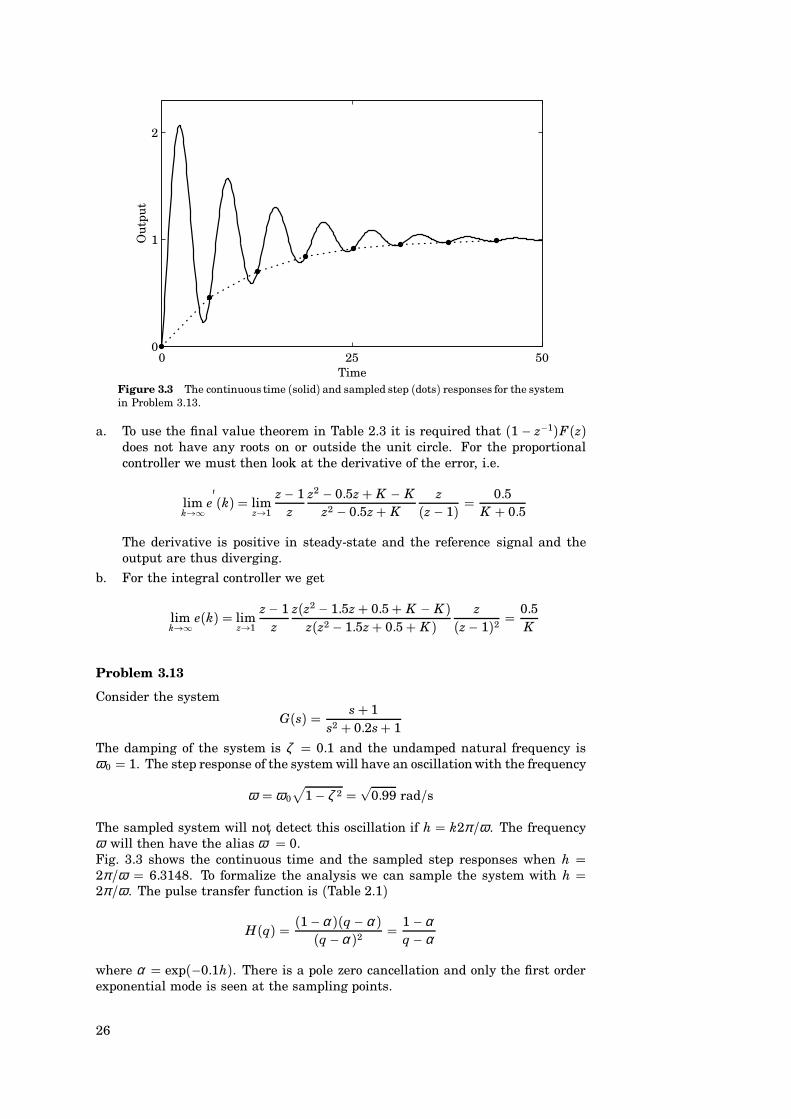
Problem 3.13
Consider the system
G(s) s+ 1s2 + 0.2s+ 1
The damping of the system is ζ 0.1 and the undamped natural frequency isω0 1. The step response of the system will have an oscillation with the frequency
ω ω0
√1− ζ 2
√0.99 rad/s
The sampled system will not detect this oscillation if h k2π/ω . The frequencyω will then have the alias ω′ 0.Fig. 3.3 shows the continuous time and the sampled step responses when h 2π/ω 6.3148. To formalize the analysis we can sample the system with h 2π/ω . The pulse transfer function is (Table 2.1)
H(q) (1−α )(q− α )(q−α )2 1 −α
q− α
where α exp(−0.1h). There is a pole zero cancellation and only the first orderexponential mode is seen at the sampling points.
26
−3 −2 −1 0 1
−2
−1
0
1
2
Re
Im
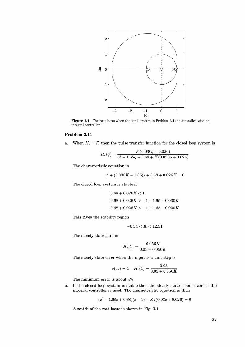
Figure 3.4 The root locus when the tank system in Problem 3.14 is controlled with anintegral controller.
Problem 3.14
a. When Hr K then the pulse transfer function for the closed loop system is
Hc(q) K (0.030q+ 0.026)q2 − 1.65q+ 0.68+ K (0.030q+ 0.026)
The characteristic equation is
z2 + (0.030K − 1.65)z+ 0.68+ 0.026K 0
The closed loop system is stable if
0.68+ 0.026K < 1
0.68+ 0.026K > −1− 1.65+ 0.030K
0.68+ 0.026K > −1+ 1.65− 0.030K
This gives the stability region
−0.54 < K < 12.31
The steady state gain is
Hc(1) 0.056K0.03+ 0.056K
The steady state error when the input is a unit step is
e(∞) 1− Hc(1) 0.030.03+ 0.056K
The minimum error is about 4%.
b. If the closed loop system is stable then the steady state error is zero if theintegral controller is used. The characteristic equation is then
(z2 − 1.65z+ 0.68)(z− 1) + K z(0.03z+ 0.026) 0
A scetch of the root locus is shown in Fig. 3.4.
27
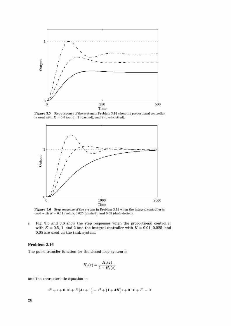
0 250 5000
1O
utp
ut
TimeFigure 3.5 Step response of the system in Problem 3.14 when the proportional controlleris used with K 0.5 (solid), 1 (dashed), and 2 (dash-dotted).
0 1000 20000
1
Ou
tpu
t
TimeFigure 3.6 Step response of the system in Problem 3.14 when the integral controller isused with K 0.01 (solid), 0.025 (dashed), and 0.05 (dash-dotted).
c. Fig. 3.5 and 3.6 show the step responses when the proportional controllerwith K 0.5, 1, and 2 and the integral controller with K 0.01, 0.025, and0.05 are used on the tank system.
Problem 3.16
The pulse transfer function for the closed loop system is
Hc(z) Ho(z)1+ Ho(z)
and the characteristic equation is
z2 + z+ 0.16+ K (4z+ 1) z2 + (1+ 4K )z+ 0.16+ K 0
28
Using the conditions in Example 3.2 give
0.16+ K < 1
0.16+ K > −1+ 1+ 4K
0.16+ K > −1 − 1 − 4K
This impliesK < 0.84
K < 0.163
0.053
K > −2.165
−0.432
Since it is assumed that K > 0 we get the condition
0 < K < 0.053
for stability.
Problem 3.17
Using (3.17) we find that the transformation is given by
Tc Wc W−1c
where Wc is the controllability matrix of the original system and Wc is the con-trollability of the transformed system.
Wc Γ ΦΓ
3 11
4 11
The pulse transfer function of the system is
H(z) C[zI − Φ]−1Γ 5 6
z− 1 −2
−1 z− 2
−1 3
4
39z+ 4
z2 − 3z
Thus the transformed system is given by
Φ 3 0
1 0
Γ 1
0
C 39 4
and
Wc Γ ΦΓ
1 3
0 1
The transformation to give the controllable form is thus
Tc 1 3
0 1
3 11
4 11
−1
111
1 2
4 −3
In the same way the tranformation to the observable form is given by
To W−1o Wo
1 0
3 1
−1 5 6
11 22
5 6
−4 4
29
Probem 3.18
a) i Poles are mapped as z esh. This mapping maps the left halfplane on the unit circle.
b) i see a)c) iii When a system with relative degree > 1, “new” zeros appear
as described on p. 63 CCS.These zeros may very well be outside the unit circle.
d) iii See Example 2.18 p. 65 CCCe) ii Sample the harmonic oscillator, Example A.3 p. 530 CCS.
For h 2π/ω AΦ 1 0
0 1
not controllable
f) ii See e)g) iii See p. 63, CCS
Problem 3.19
a. The controllability matrix is
Wc Γ ΦΓ Φ2Γ
0 1 0
1 2 0
2 3 0
Since one column is zero we find that the system is not reachable (det Wc0),see Theorem 3.7.
b. The system may be controllable if the matrix Φ is such that Φnx(0) 0. Inthis case
Φ3
0 0 0
0 0 0
0 0 0
and the origin can be reached from any initial condition x(0) by the controlsequence u(0) u(1) u(2) 0.
Probem 3.20
Ho 1q2 + 0.4q
Hr K
a.Htot Hr Ho
1+ Hr Ho K
q2 + 0.4q+ KThe system is stable if, see p. 82,
K < 1
K > −1+ 0.4K > −1 − 0.4
⇒ −0.6 < K < 1
b.e(k) uc − y
E(z) (
1 − Htot(z))
Uc(z)If K is chosen such that the closed loop system is stable (e.g. K 0.5) thefinal-value theorem can be used.
limk→∞
e(k) limz→1
z− 1z
E(z) limz→1
z− 1z
(1 − K
z2 + 0.4z+ K
) zz− 1
limz→1
z2 + 0.4zz2 + 0.4z+ K
1.41.4+ K
0.74A K 0.5
30
−2 0 2−2
0
2
Re
Im
Figure 3.7 The root locus for Problem 3.21b.
Problem 3.21
y(k) 0.4q+ 0.8q2 − 1.2q+ 0.5
u(k)
a.
Htot Hr Ho
1+ Hr Ho (0.4q+ 0.8)K
q2 − 1.2q+ 0.5+ K (0.4q+ 0.8)
(0.4q+ 0.8)Kq2 + q(0.4K − 1.2) + 0.5+ 0.8K
The system is stable if, see p. 82 CCS,
0.5+ 0.8K < 1 ⇒ K < 0.625
0.5+ 0.8K > −1+ 0.4K − 1.2 ⇒ K > −6.75
0.5+ 0.8K > −1 − 0.4K + 1.2 ⇒ K > −0.25
−0.25 < K < 0.625
b.Hr K
q
Htot Hr Ho
1+ Hr Ho (0.4q+ 0.8)K
q(q2 − 1.2q+ 0.5) + K (0.4q+ 0.8)
(0.4q+ 0.8)Kq3 − 1.2q2+ q(0.5+ 0.4K ) + 0.8K
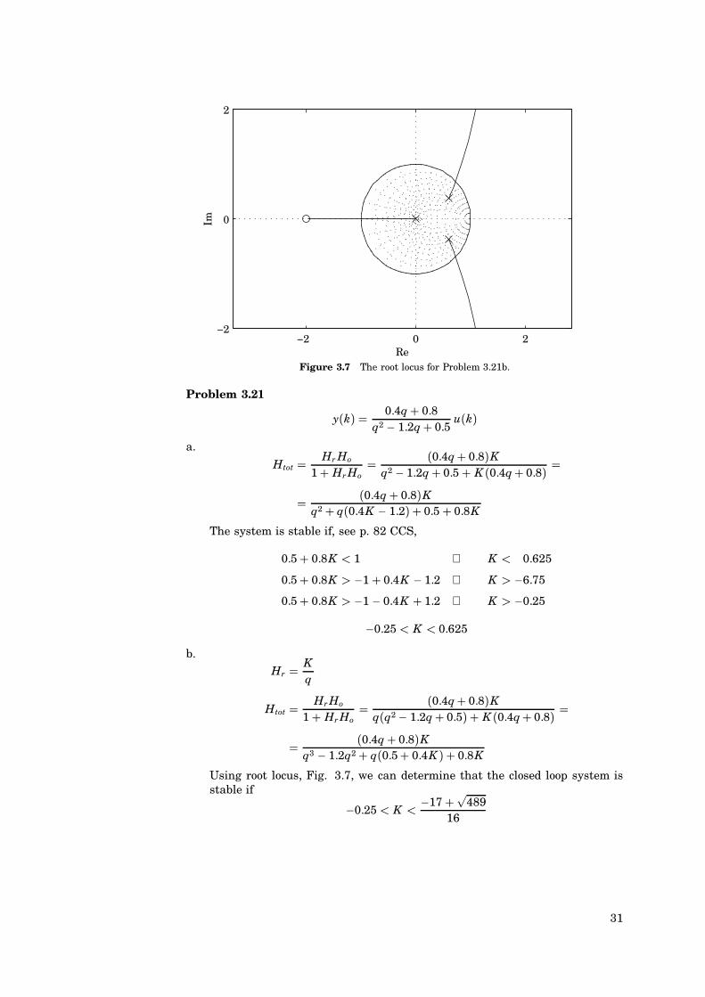
Using root locus, Fig. 3.7, we can determine that the closed loop system isstable if
−0.25 < K < −17+√48916
31
Solutions to Chapter 4
Problem 4.1
The characteristic equation of the closed loop system is
det(zI − (Φ − ΓL)) z2 − (a11 + a22 − b2X2 − b1X1)z+ a11a22 − a12a21
+ (a12b2 − a22b1)X1 + (a21b1 − a11b2)X2
Identifying with the desired characteristic equation gives b1 b2
a12b2 − a22b1 a21b1 − a11b2
X1
X2
p1 + tr Φp2 − det Φ
where tr Φ a11 + a22 and det Φ a11a22 − a12a21. The solution is X1
X2
1∆
a21b1 − a11b2 −b2
−a12b2 + a22b1 b1
p1 + tr Φp2 − det Φ
where
∆ a21b21 − a12b2
2 + b1b2(a22 − a11)To check when ∆ 6 0 we form the controllability matrix of the system
Wc Γ ΦΓ
b1 a11b1 + a12b2
b2 a21b1 + a22b2
and we find that
∆ det Wc
There exists a solution to the system of equations above if the system is control-lable. For the double integrator with h 1 and dead beat response we havea11 a12 a22 b2 1, a21 0, b1 0.5, and p1 p2 0.This gives X1
X2
(−1) −1 −1
−0.5 −0.5
2
−1
1
1.5
This is the same as given in Example 4.4.
Problem 4.2
In this case the desired characteristic equation is
(z− 0.1)(z− 0.25) z2 − 0.35z+ 0.025.
Using the result from Problem 4.1 we find that
∆ 0.5
and L is obtained from
LT X1
X2
1∆
0.5 0
0.1 1
0.75
−0.025
0.75
0.1
To check the result we form
Φ − ΓL 1 0.1
0.5 0.1
− 0.75 0.1
0 0
0.25 0
0.5 0.1
The matrix Φ − ΓL thus has the desired eigenvalues 0.25 and 0.1.
32
0 1 2 3 4 5
−2
0
Ou
tpu
t u
(0)
Sampling period hFigure 4.1 u(0) s function of h in Problem 4.3.
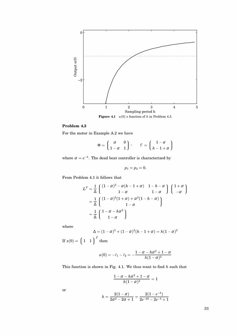
Problem 4.3
For the motor in Example A.2 we have
Φ α 0
1 − α 1
A Γ 1 −α
h− 1+α
where α e−h. The dead beat controller is characterized by
p1 p2 0.
From Problem 4.1 it follows that
LT 1∆
(1− α )2 −α (h− 1+α ) 1− h− α1 −α 1 −α
1+α−α
1
∆
(1− α )2(1+α ) +α 2(1− h− α )1− α
1
∆
1 −α − hα 2
1− α
where
∆ (1 −α )3 + (1 −α )2(h− 1+α ) h(1−α )2
If x(0) 1 1
Tthen
u(0) −X1 − X2 −1 −α − hα 2 + 1 −αh(1−α )2
This function is shown in Fig. 4.1. We thus want to find h such that
1 −α − hα 2 + 1 −αh(1−α )2 1
or
h 2(1−α )2α 2 − 2α + 1
2(1− e−h)2e−2h − 2e−h + 1
33
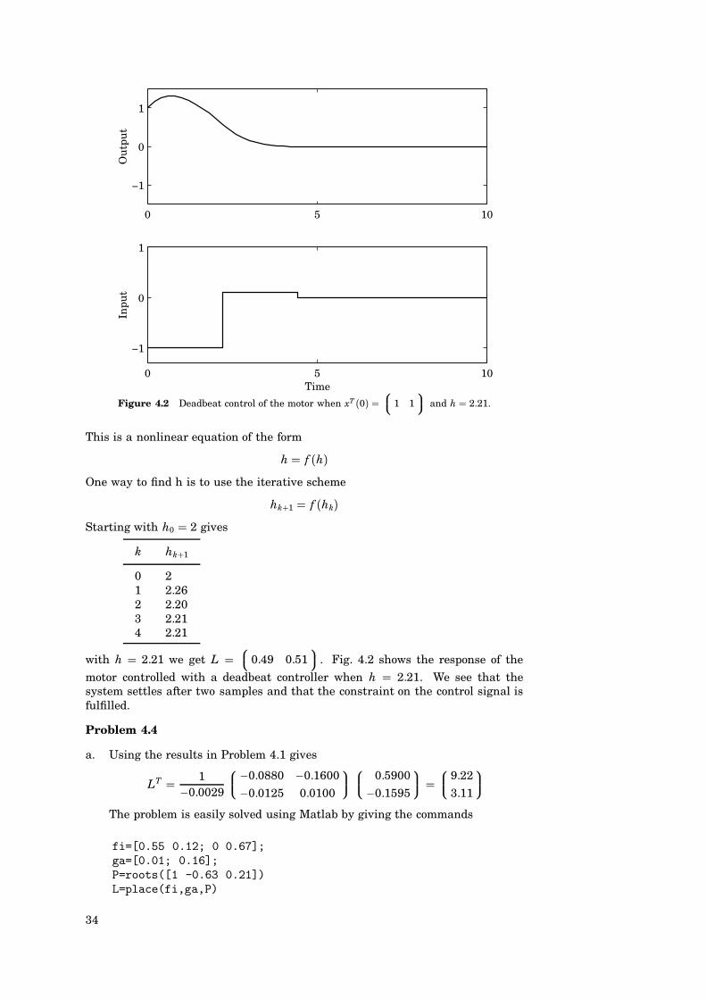
0 5 10
−1
0
1O
utp
ut
0 5 10
−1
0
1
Inpu
t
Time
Figure 4.2 Deadbeat control of the motor when xT (0) 1 1
and h 2.21.
This is a nonlinear equation of the form
h f (h)One way to find h is to use the iterative scheme
hk+1 f (hk)Starting with h0 2 gives
k hk+1
0 21 2.262 2.203 2.214 2.21
with h 2.21 we get L 0.49 0.51
. Fig. 4.2 shows the response of the
motor controlled with a deadbeat controller when h 2.21. We see that thesystem settles after two samples and that the constraint on the control signal isfulfilled.
Problem 4.4
a. Using the results in Problem 4.1 gives
LT 1−0.0029
−0.0880 −0.1600
−0.0125 0.0100
0.5900
−0.1595
9.22
3.11
The problem is easily solved using Matlab by giving the commands
fi=[0.55 0.12; 0 0.67];ga=[0.01; 0.16];P=roots([1 -0.63 0.21])L=place(fi,ga,P)
34
0 2 4
0
1
Ou
tpu
t
0 2 4−15
−10
−5
0
5
Inpu
t
TimeFigure 4.3 The response and the control signal of the system in Problem 4.4 when
x(0) 1 0
T
and L 9.22 3.11
.
b. From Example 4.4 we find that the continuous-time characteristic polynomials2 + 2ζ ω s +ω2 corresponds to z2 + p1z+ p2 with
p1 −2e−ζ ω h cos(ωh√
1 − ζ 2) −0.63
p2 e−2ζ ω h 0.21
This has the solution ζ 0.7 and ω 5.6, so the characteristic polynomialbecomes s2 + 7.8s+ 31.7. In Matlab you can dord=roots([1-0.63 0.21])rc=Log(rd)/hAc=poly(rc)
The chosen sampling interval is higher than recommended by the rule ofthumb, since
ωh 1.1 > 0.6
c. The closed loop system when using L 9.22 3.11
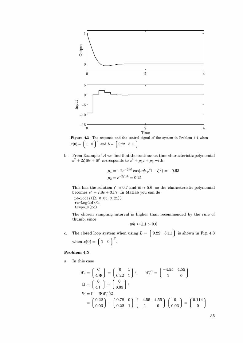
is shown in Fig. 4.3
when x(0) 1 0
T.
Problem 4.5
a. In this case
Wo C
CΦ
0 1
0.22 1
A W−1o
−4.55 4.55
1 0
Ω
0
CΓ
0
0.03
AΨ Γ − ΦW−1
o Ω
0.22
0.03
− 0.78 0
0.22 1
−4.55 4.55
1 0
0
0.03
0.114
0
35
We get
x(k) ΦW−1o
y(k− 1)y(k)
+Ψu(k− 1)
−3.55 3.55
0 1
y(k − 1)y(k)
+0.114
0
u(k− 1)
b. The dynamical observer (4.28) has the form
x(k+ 1jk) (Φ − K C)x(kjk− 1) + Γu(k)+ K y(k).
In this case we choose K such that the eigenvalues of Φ − K C are in theorigin. Using the results from Problem 4.1 but with ΦT and CT instead of Φand Γ gives
K 2.77
1.78
c. The reduced order observer (4.32) has the form
x(kjk) (I − K C)(Φ x(k− 1jk− 1) + Γu(k− 1)) + K y(k).
In this case we want to find K such that
i. C K 1
ii. (I − K C)Φ has eigenvalues in the origin. The first condition implies thatk2 1. Further
(I − K C)Φ 1 −k1
0 0
0.78 0
0.22 0
0.78− 0.22k1 −k1
0 0
The eigenvalues will be in the origin if
k1 0.78/0.22 3.55.
The observer is then
x(kjk) 0 −3.55
0 0
x(k− 1jk− 1) + 0.114
0
u(k− 1) + 3.55
1
y(k)
Since x2(kjk) y(k) we get
x(kjk) −3.55 3.55
0 1
y(k− 1)y(k)
+ 0.114
0
u(k− 1)
which is the same as the observer obtained by direct calculation.
Problem 4.6
From Problem 2.10 we get for h 12
x(kh+ h) 0.790 0
0.176 0.857
x(kh) + 0.281
0.0296
u(kh)
y(kh) 0 1
x(kh)
The continuous time poles of the system are −0.0197 and −0.0129. The observershould be twice as fast as the fastest mode of the open loop system. We thuschoose the poles of the observer in
z e−0.0394⋅12 0.62
36
0 250 500−0.5
0
0.5
1
x1 a
nd
xe1
0 250 500−0.5
0
0.5
1
x2 a
nd
xe2
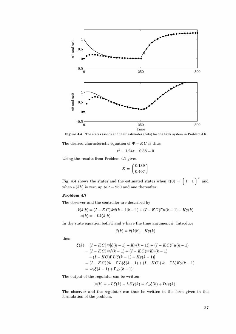
TimeFigure 4.4 The states (solid) and their estimates (dots) for the tank system in Problem 4.6
The desired characteristic equation of Φ − K C is thus
z2 − 1.24z+ 0.38 0
Using the results from Problem 4.1 gives
K 0.139
0.407
Fig. 4.4 shows the states and the estimated states when x(0)
1 1T
and
when u(kh) is zero up to t 250 and one thereafter.
Problem 4.7
The observer and the controller are described by
x(kjk) (I − K C)Φ x(k− 1jk− 1) + (I − K C)Γu(k− 1) + K y(k)u(k) −Lx(kjk).
In the state equation both x and y have the time argument k. Introduce
ξ (k) x(kjk)− K y(k)then
ξ (k) (I − K C)Φ[ξ (k − 1) + K y(k− 1)] + (I − K C)Γu(k− 1) (I − K C)Φξ (k− 1) + (I − K C)ΦK y(k− 1)− (I − K C)ΓL[ξ (k − 1) + K y(k− 1)]
(I − K C)(Φ − ΓL)ξ (k − 1) + (I − K C)(Φ − ΓL)K y(k − 1) Φoξ (k − 1) + Γo y(k− 1)
The output of the regulator can be written
u(k) −Lξ (k) − LK y(k) Coξ (k) + Do y(k).The observer and the regulator can thus be written in the form given in theformulation of the problem.
37
Problem 4.8
The constant disturbance v(k) can be described by the dynamical system
w(k+ 1) w(k)v(k) w(k)
The process can thus be described on the form given in (4.43) with
Φw 1A Φxw 1
0
a. If the state and v can be measured then we can use the controller
u(k) −Lx(k) − Lww(k).This gives the closed loop system
x(k+ 1) Φx(k) + Φxww(k)− ΓLx(k) − ΓLww(k) (Φ − ΓL)x(k) + (Φxw − ΓLw)w(k)
y(k) C x(k)In general it is not possible to totally eliminate the influence of w(k). This isonly possible if Φxw−ΓLw is the zero matrix. We will therefore only considerthe situation at the output in steady state
y(∞) C[I − (Φ − ΓL)]−1(Φxw − ΓLw)w(∞) Hw(1)w(∞)The influence of w (or v) can be zero in steady state if
Hw(1) 0
This will be the case if
Lw 1 − ϕ c22
γ 1(1− ϕ c22) + γ 2ϕ c12
where ϕ cij is the (iA j) element of Φ − ΓL and γ i is the i:th element of Γ.Assume that L is determined to give a dead beat regulator then
L 3.21 5.57
and
Φ − ΓL −0.142 −0.114
0.179 0.142
and
Lw 5.356
b. In this case is the state but not the disturbance measurable. The disturbancecan now be calculated from the state equation
Φxww(k− 1) x(k)− Φx(k − 1)− Γu(k− 1).The first element in this vector equation gives
w(k− 1) [1 0](x(k)− Φx(k− 1)− Γu(k − 1))Since w(k) is constant and x(k) is measurable it is possible to calculate w(k) w(k− 1). The following control law can now be used
u(k) −Lx(k) − Lww(k)where Lw is the same as in (a). Compared with the controller in (a) there isa delay in the detection of the disturbance.
38
0 5 10 15−0.2
0
0.2
Out
put
0 5 10 15−2
0
2
Out
put
0 5 10 15−2
0
2O
utpu
t
Time0 5 10 15
0
2
Est
imat
e ve
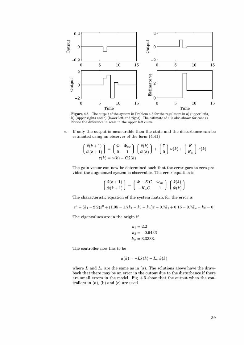
TimeFigure 4.5 The output of the system in Problem 4.8 for the regulators in a) (upper left),b) (upper right) and c) (lower left and right). The estimate of v is also shown for case c).Notice the difference in scale in the upper left curve.
c. If only the output is measurable then the state and the disturbance can beestimated using an observer of the form (4.41) x(k+ 1)
w(k+ 1)
Φ Φxw
0 1
x(k)w(k)
+Γ0
u(k) + K
Kw
ε (k)
ε (k) y(k)− C x(k)
The gain vector can now be determined such that the error goes to zero pro-vided the augmented system is observable. The error equation is x(k+ 1)
w(k+ 1)
Φ − K C Φxw
−KwC 1
x(k)w(k)
The characteristic equation of the system matrix for the error is
z3 + (k1 − 2.2)z2 + (1.05− 1.7k1 + k2 + kw)z+ 0.7k1 + 0.15 − 0.7kw− k2 0.
The eigenvalues are in the origin if
k1 2.2k2 −0.6433
kw 3.3333.
The controller now has to be
u(k) −Lx(k)− Lww(k)
where L and Lv are the same as in (a). The solutions above have the draw-back that there may be an error in the output due to the disturbance if thereare small errors in the model. Fig. 4.5 show that the output when the con-trollers in (a), (b) and (c) are used.
39

Problem 4.9
a. The state equation for the tank system when h 12 was given in the solutionto Problem 4.6. The desired characteristic equation is
z2 − 1.55z+ 0.64 0
Using the result in Problem 9.1 give
L 0.251 0.8962
b. An integrator can be incorporated as shown in Section 4.5 by augmenting the
system withx3(kh+ h) x3(kh) + uc(kh)− C x(kh)
and using the control law
u(kh) −Lx(kh) − X3x3(kh)+ Xcuc(k)
The closed loop system is then x(k+ 1)x3(k+ 1)
0.790− 0.281X1 −0.281X2 −0.281X3
0.176− 0.0296X1 0.857− 0.0296X2 −0.0296X3
0 −1 1
x(k)
x3(k)
+
0.281Xc
0.0296Xc
1
uc(k)
The characteristic equation is
z3 + (−2.647+ 0.281X1+ 0.0296X2)z2
+ (2.3240− 0.5218X1 − 0.0035X2 − 0.0296X3)z++ (−0.6770+ 0.2408X1 − 0.0261X2 − 0.0261X3) 0
Assume that two poles are placed in the desired location and that the thirdpole is in p. We get the following system of equations to determine the statefeedback vector.
0.281 0.0296 0
−0.5218 −0.0035 −0.0296
0.2408 −0.0261 −0.0261
X1
X2
X3
2.647− 1.55− p
−2.3240+ 1.55p+ 0.64
0.6770− 0.64p
This gives
X1
X2
X3
3.279− 3.028p
5.934− 5.038p
−1.617+ 1.617p
c. The parameter Xc will not influence the characteristic equation, but it is a
feedforward term from the reference signal, see Fig. 4.11 CCS. Fig. 4.6 showsthe step response for some values of p. Fig. 4.7 shows the influence of Xc whenp 0.
40
0 250 5000
1
Ou
tpu
t
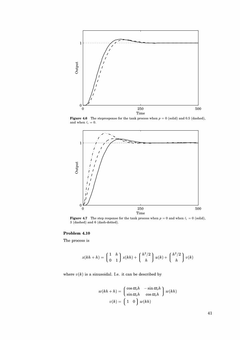
TimeFigure 4.6 The stepresponse for the tank process when p 0 (solid) and 0.5 (dashed),and when Xc 0.
0 250 5000
1
Ou
tpu
t
TimeFigure 4.7 The step response for the tank process when p 0 and when Xc 0 (solid),3 (dashed) and 6 (dash-dotted).
Problem 4.10
The process is
x(kh+ h) 1 h
0 1
x(kh) + h2/2
h
u(k)+h2/2
h
v(k)
where v(k) is a sinusoidal. I.e. it can be described by
w(kh+ h) cosω oh − sinω oh
sinω oh cosω oh
w(kh)
v(k) 1 0
w(kh)
41
The augmented system (9.33) is now
x(kh+ h)w(kh+ h)
1 h h2/2 0
0 1 h 0
0 0 α −β0 0 β α
x(kh)
w(kh)
+
h2/2h
0
0
u(kh)
where α cosω oh and β sinω oh. Assume first that the control law is
u(kh) −Lx(kh) − Lww(kh)
whereL
1h2
32h
i.e., a dead beat controller for the states. Further if Lw
1 0 we would
totally eliminate v since v and u are influencing the system in the same way.Compare the discussion in the solution of Problem 4.8.Since x(kh) and ξ (kh) cannot be measured we use the observer of the structure(9.35) where
Φxw h2/2 0
h 0
and Φw α −β
β α
The error equation is then x(k+ 1)
w(k+ 1)
Φ − K C Φxw
−KwC 1
x(k)w(k)
1 − k1 h h2/2 0
−k2 1 h 0
−kw1 0 α −β−kw2 0 β α
x(k)
w(k)
Let the desired characteristic equation of the error be
(z− γ )4 0
If h 1 and ω o 0.1π then for γ 0.5 we get the following system of equations1 0 0 0
−2.9022 1 0.5 0
2.9022 −1.9022 0.0245 −0.1545
−1 1 −0.4756 −0.1545
k1
k2
kw1
kw2
−4γ + 3.9022
6γ 2 − 5.8044
−4γ 3 − 3.9022
γ 4 − 1
which has the solution
k1 1.9022
k2 1.1018
kw1 0.2288
kw2 0.1877
Fig. 9.8 shows the states of the double integrator and their estimates when v(t) sin(ω ot). It is seen that the controller is able to eliminate the disturbance.
Problem 4.11
We have to determine the feedback vector L such that
42
0 10 20 30−2
0
2
x1 a
nd
xe1
0 10 20 30−2
0
2
x2 a
nd
xe2
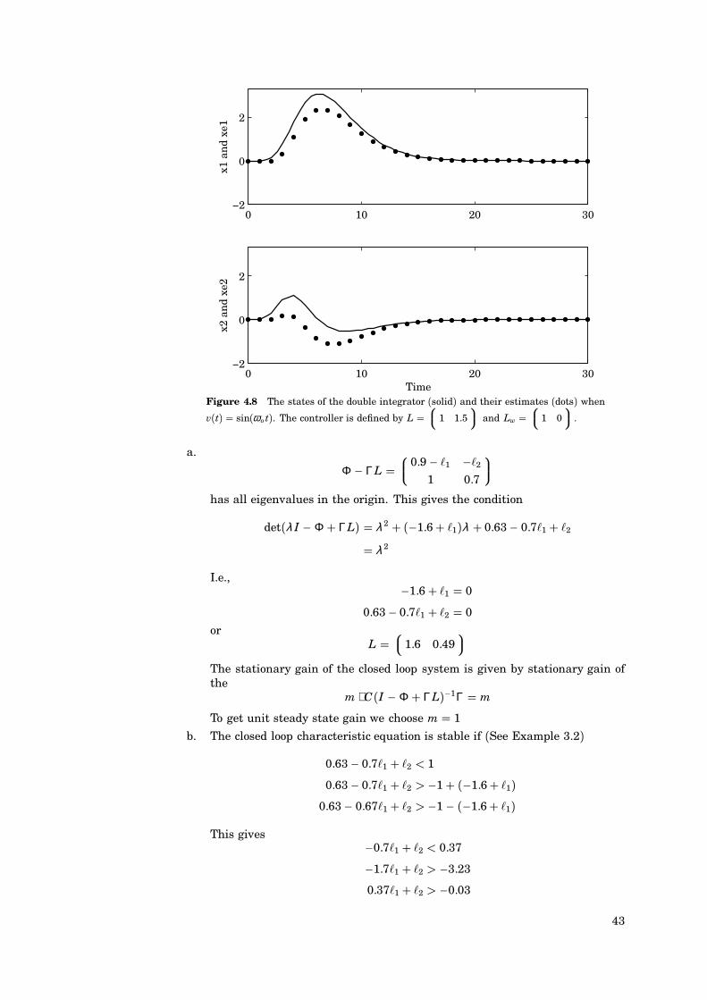
TimeFigure 4.8 The states of the double integrator (solid) and their estimates (dots) when
v(t) sin(ω o t). The controller is defined by L 1 1.5
and Lw 1 0
.
a.
Φ − ΓL 0.9 − X1 −X2
1 0.7
has all eigenvalues in the origin. This gives the condition
det(λ I − Φ + ΓL) λ 2 + (−1.6+ X1)λ + 0.63− 0.7X1 + X2
λ 2
I.e.,−1.6+ X1 0
0.63− 0.7X1 + X2 0
orL
1.6 0.49
The stationary gain of the closed loop system is given by stationary gain ofthe
m ⋅ C(I − Φ + ΓL)−1Γ m
To get unit steady state gain we choose m 1
b. The closed loop characteristic equation is stable if (See Example 3.2)
0.63− 0.7X1 + X2 < 1
0.63− 0.7X1 + X2 > −1+ (−1.6+ X1)0.63− 0.67X1 + X2 > −1 − (−1.6+ X1)
This gives−0.7X1 + X2 < 0.37
−1.7X1 + X2 > −3.23
0.37X1 + X2 > −0.03
43
3
2
1
1
1 2 3
Deadbeat
1
2l
l
−
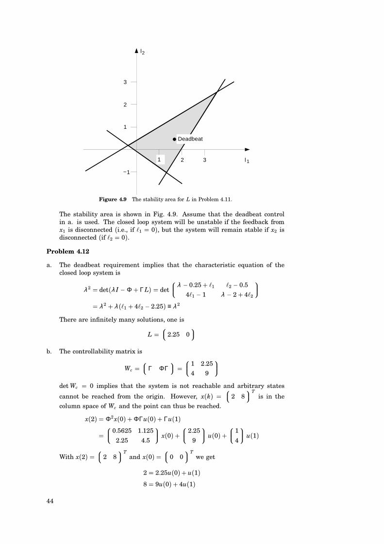
Figure 4.9 The stability area for L in Problem 4.11.
The stability area is shown in Fig. 4.9. Assume that the deadbeat controlin a. is used. The closed loop system will be unstable if the feedback fromx1 is disconnected (i.e., if X1 0), but the system will remain stable if x2 isdisconnected (if X2 0).
Problem 4.12
a. The deadbeat requirement implies that the characteristic equation of theclosed loop system is
λ 2 det(λ I − Φ + ΓL) det λ − 0.25+ X1 X2 − 0.5
4X1 − 1 λ − 2+ 4X2
λ 2 + λ (X1 + 4X2 − 2.25) ≡ λ 2
There are infinitely many solutions, one is
L 2.25 0
b. The controllability matrix is
Wc Γ ΦΓ
1 2.25
4 9
det Wc 0 implies that the system is not reachable and arbitrary states
cannot be reached from the origin. However, x(k) 2 8
Tis in the
column space of Wc and the point can thus be reached.
x(2) Φ2x(0) + ΦΓu(0) + Γu(1)
0.5625 1.125
2.25 4.5
x(0) + 2.25
9
u(0) + 1
4
u(1)
With x(2) 2 8
Tand x(0)
0 0T
we get
2 2.25u(0)+ u(1)8 9u(0) + 4u(1)
44

One solution isu(0) 0
u(1) 2
c. The observer should have the characteristic equation
(λ − 0.2)2 λ 2 − 0.4λ + 0.04 0
det(λ I − Φ + K C) det λ + k1 − 0.25 −0.5
k2 − 1 λ − 2
λ 2 + (k1 − 2.25)λ + 0.5k2 − 2k1
Identifying coefficients give the system
k1 − 2.25 −0.4
0.5k2 − 2k1 0.04
which has the solution
K 1.85
7.48
45
Solutions to Chapter 5
Problem 5.1
Euclid’s algorithm defines a sequence of polynomials A0A ( ( ( A An where A0 A,A1 B and
Ai Ai+1 Qi+1 + Ai+2
If the algorithm terminates with An+1 then the greatest common factor is An. Forthe polynomials in the problem we get
A0 z4 − 2.6z3 + 2.25z2 − 0.8z+ 0.1
A1 z3 − 2z2 + 1.45z− 0.35.
This gives
Q1 z− 0.6
A2 −0.4z2 + 0.42z− 0.11 −0.4(z2 − 1.05z+ 0.275)
The next step of the algorithm gives
Q2 (z− 0.95)/(−0.4)A3 0.1775z− 0.08875 0.1775(z− 0.5)
FinallyQ3 (z− 0.55)/0.1775
A4 0
The greatest common factor of A and B is thus z− 0.5.
Problem 5.2
a. To use Algorithm 5.1 we must know the pulse-transfer function B(z)/A(z)and the desired closed-loop characteristic polynomial Acl(z). Since the desiredpulse-transfer function from uc to y is Hm(z) (1+α )/(z+α ), we know atleast that (z+α ) must be a factor in Acl(z).Step 1. You easily see that, with A and Acl being first order polynomials andB a scalar, you can solve the equation for the closed loop system using scalarsR(z) r0 and S(z) s0:
A(z)R(z) + B(z)S(z) Acl(z)(z+ a) ⋅ r0 + 1 ⋅ s0 z+α
Identification of coefficients gives the following equation system:r0 1
ar0 + s0 α
with the solution r0 1 and s0 α − a.
46
Step 2. Factor Acl(z) as Ac(z)Ao(z) where deg Ao ≤ deg R 0. Thus, Ao 1and Ac z+α . Choose
T(z) t0Ao(z) Ac(1)B(1) Ao(z) 1+α
With this choice of T , the static gain from uc to y is set to 1 (Hm(1) 1), andthe observer dynamics are cancelled in the pulse-transfer function from uc toy. In this case, there are no observer dynamics, though, since deg Ao 0.
The resulting control law becomes
R(q)u(k) T(q)uc(k)− S(q)y(k)u(k) (1+α )uc(k)− (α − a)y(k)
i.e., a (static) proportional controller.
Solution with higher order observer: The solution above is not the onlyone solving the original problem. We can, for example, decide to have anotherclosed loop pole in z −β , say.
Step 1. To solve the equation for the closed loop characteristic polynomial wemust increase the order of R by one. This gives
(z+ a)(r0z+ r1) + 1 ⋅ s0 (z+α )(z+ β )and the equation system becomes
r0 1
ar0 + r1 α + βar1 + s0 αβ
⇐⇒
r0 1
r1 α + β − a
s0 αβ − a(α + β − a)
Step 2. Splitting Acl into factors Ao z+ β and Ac z+α gives
T(z) t0 Ao(z) Ac(1)B(1) Ao(z) (1+α )(z+ β )
The resulting control law becomes
R(q)u(k) T(q)uc(k)− S(q)y(k) ⇒
u(k) −(
α + β − a)
u(k− 1) +(
1+α)(
uc(k)+ β uc(k− 1))
−(
αβ − a(α + β − a))
y(k− 1)
The controller thus is a dynamical system. In this case there is a delay ofone sample from the measurements y to the control signal u. This could havebeen avoided by choosing deg S 1.
b. The closed loop characteristic polynomial is given by AR+B S, i.e. (z+α ) inthe first solution, and (z+α )(z+ β ) in the second one. In both cases we getthe same closed loop pulse-transfer function from uc to y since the observerpolynomial is cancelled by T(z):
Hm(z) B(z)T(z)A(z)R(z)+ B(z)S(z)
t0 B(z)Ac(z)
1+αz +α
Fig. 5.1 shows the response when the two different controllers are used. It isassumed in the simulations that a −0.99, and that the design parametersare α −0.7 and β −0.5. You can see the effect of the observer polynomialwhen regulating a nonzero initial state, but not in the response to a set pointchange.
47
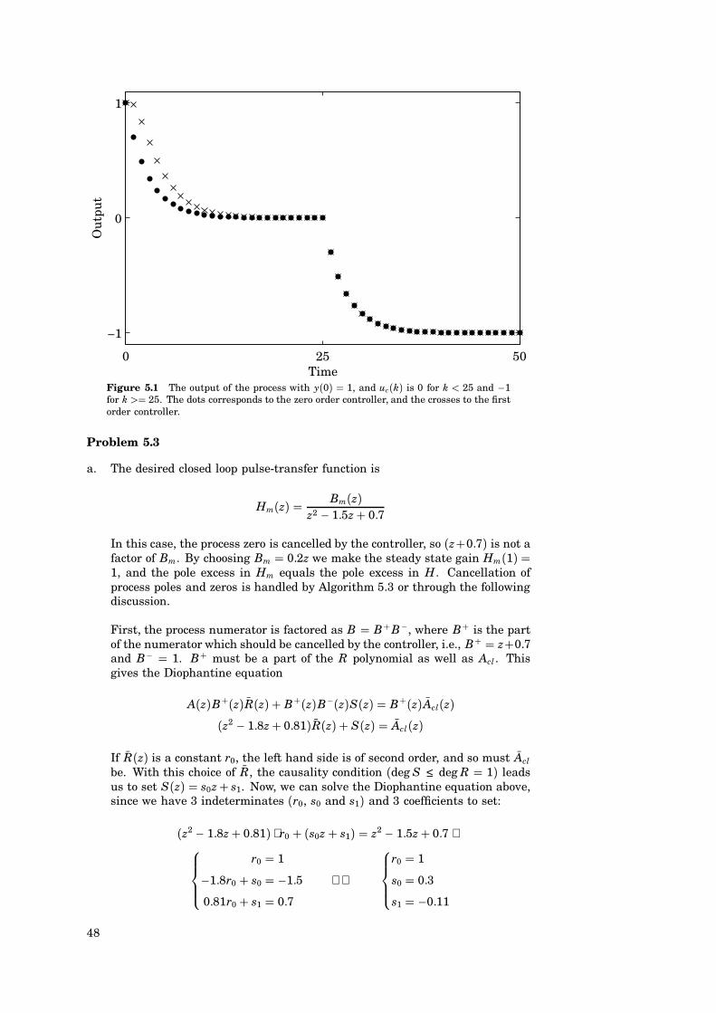
0 25 50
−1
0
1O
utpu
t
TimeFigure 5.1 The output of the process with y(0) 1, and uc(k) is 0 for k < 25 and −1for k > 25. The dots corresponds to the zero order controller, and the crosses to the firstorder controller.
Problem 5.3
a. The desired closed loop pulse-transfer function is
Hm(z) Bm(z)z2 − 1.5z+ 0.7
In this case, the process zero is cancelled by the controller, so (z+0.7) is not afactor of Bm. By choosing Bm 0.2z we make the steady state gain Hm(1) 1, and the pole excess in Hm equals the pole excess in H. Cancellation ofprocess poles and zeros is handled by Algorithm 5.3 or through the followingdiscussion.
First, the process numerator is factored as B B+B−, where B+ is the partof the numerator which should be cancelled by the controller, i.e., B+ z+0.7and B− 1. B+ must be a part of the R polynomial as well as Acl . Thisgives the Diophantine equation
A(z)B+(z)R(z) + B+(z)B−(z)S(z) B+(z)Acl(z)(z2 − 1.8z+ 0.81)R(z) + S(z) Acl(z)
If R(z) is a constant r0, the left hand side is of second order, and so must Acl
be. With this choice of R, the causality condition (deg S ≤ deg R 1) leadsus to set S(z) s0z+ s1. Now, we can solve the Diophantine equation above,since we have 3 indeterminates (r0, s0 and s1) and 3 coefficients to set:
(z2 − 1.8z+ 0.81) ⋅ r0 + (s0z+ s1) z2 − 1.5z+ 0.7 ⇒r0 1
−1.8r0 + s0 −1.5
0.81r0 + s1 0.7
⇐⇒
r0 1
s0 0.3
s1 −0.11
48
Thus, we have R(z) B+(z)R(z) z+ 0.7 and S(z) 0.3z− 0.11. To obtainthe desired
Hm(z) BTAR + B S
B+B−TB+(z2 − 1.5z+ 0.7)
0.2zz2 − 1.5z+ 0.7
we must selectT(z) 0.2z
The controller is now
u(k) −0.7u(k− 1) + 0.2uc(k)− 0.3y(k)+ 0.11y(k− 1).
b. In this case we do not want to cancel the process zero, so
Hm(z) Bm(z)z2 − 1.5z+ 0.7
0.21.7 (z+ 0.7)
z2 − 1.5z+ 0.7
in order to get Hm(1) 1. The closed loop characteristic polynomial is nowgiven by the identity
(z2 − 1.8z+ 0.81)R(z)+ (z+ 0.7)S(z) Acl(z)
The simplest choice, a zero order controller, will not suffice in this case sinceit would only give 2 parameters r0 and s0 to select the 3 parameters in thesecond order polynomial z2 − 1.5z+ 0.7. Thus, we must increase the order ofthe controller by one and, consequently, add an observer pole which is placedat the origin, i.e. Ao z and Acl z3 − 1.5z2 + 0.7z. Letting
R r0z+ r1
S s0z+ s1
the identity then gives the system of equationsr0 1
−1.8r0 + r1 + s0 −1.50.81r0 − 1.8r1 + 0.7s0 + s1 0.7
0.81r1 + 0.7s1 0
⇐⇒
r0 1
r1 0.0875
s0 0.2125
s1 −0.1012
Further T t0 Ao 0.21.7 z. The controller is thus
u(k) −0.0875u(k− 1) + 0.1176uc(k)− 0.2125y(k)+ 0.1012y(k− 1)
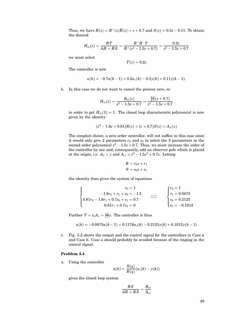
c. Fig. 5.2 shows the output and the control signal for the controllers in Case aand Case b. Case a should probably be avoided because of the ringing in thecontrol signal.
Problem 5.4
a. Using the controller
u(k) S(q)R(q)(uc(k)− y(k))
gives the closed loop system
B SAR + B S
Bm
Am
49
0 20 400
1O
utpu
t
0 20 40−0.1
0
0.1
0.2
Con
trol
Time
0 20 400
1
Out
put
0 20 40−0.1
0
0.1
0.2
Con
trol
TimeFigure 5.2 The output and the control signal for the controllers in Case a (left) andCase b (right) in Problem 5.3. The ringing in the control signal in Case a is due to thecancellation of the process zero on the negative real axis.
Section 5.10 gives one solution to the problem
R B(Am − Bm)S ABm
With the given system and model we get
R 1(z+α − 1− α ) z− 1
S (z+ a)(1+α )The controller contains an integrator. Further the pole of the process is can-celled.
b. The characteristic polynomial of the closed loop system is
AR + B S (z+α )(z+ a)The closed loop system will contain an unstable mode if jaj > 1. The controllercan be written
SR A
BBm
Am − Bm
From this we can conclude that in order to get a stable closed loop we mustfulfill the following constraints.
i. Bm must contain the zeros of B that are outside the unit circle.
ii. Am − Bm must contain the poles of the process that are outside the unitcircle. The first constraint is the same as for the polynomial design discussedin Chapter 5.
Problem 5.5
a. Equation (5.33) gives the pulse transfer operator from uc and v to y:
y(k) Bm
Amuc(k) + B R
AR + B Sv(k)
The design in Problem 5.2 gave
R 1
S α − a
50
We thus getB R
AR + B S 1
z+αIf v(k) is a step there will thus be a steady state error 1/(1+α ) in the output.
b. By inspection of the transfer function from v to y we see that we must makeR(1) 0 in order to remove the steady state error after a load disturbancestep. By forcing the factor (z− 1) into R(z) we thus have obtained integralaction in the controller. The design problem is solved by using the generalAlgorithm 5.3 or through a discussion like the one below.
With R(z) (z− 1)R(z) the closed loop characteristic equation becomes
A(z)(z− 1)R(z) + B(z)S(z) Acl(z)(z+ a)(z− 1)R(z) + 1 ⋅ S(z) Acl(z)
If R(z) is a constant r0, the left hand side is of second order, and so must Aclbe. With this choice of R, the causality condition (deg S ≤ deg R 1) leadsus to set S(z) s0z+ s1. Now, we can solve the Diophantine equation above,since we have 3 indeterminates (r0, s0 and s1) and 3 coefficients to set:
(z+ a)(z− 1) ⋅ r0 + (s0z+ s1) (z+α )(z+ β ) ⇒r0 1
(a− 1)r0 + s0 α + β
−ar0 + s1 αβ
⇐⇒
r0 1
s0 α + β − a+ 1
s1 αβ + a
To obtain the desired
Hm(z) B(z)T(z)A(z)R(z)+ B(z)S(z)
T(z)(z+α )(z+ β )
1+αz+α
we must selectT(z) (1+α )(z+ β )
The controller is now
u(k) u(k− 1)− (α + β − a+ 1)y(k)− (a+αβ )y(k − 1)+ (1+α )uc(k)+ β (1+α )uc(k − 1)
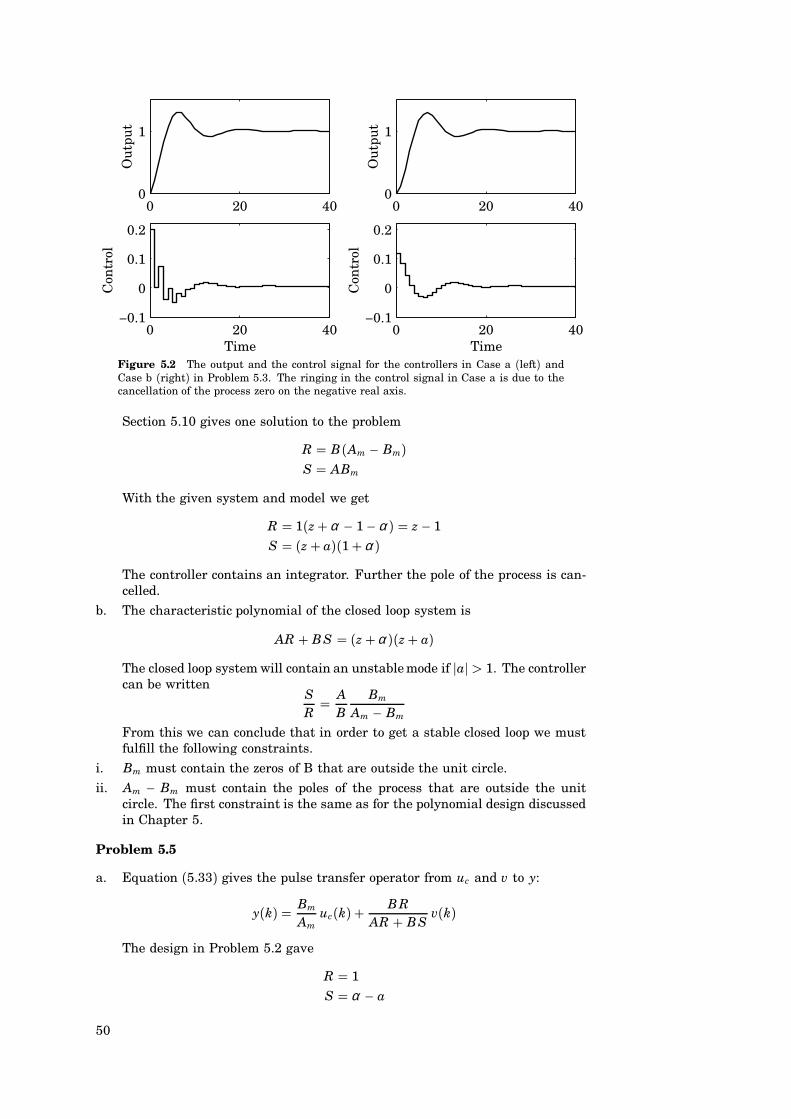
Fig. 5.3 shows the controllers in Problem 5.2 and the controller with anintegrator. The reference value is zero and there is an initial value of thestate in the process. At t 25 a constant load disturbance is introduced. It isassumed that a −0.99, and the design parameters are chosen as α −0.7and β −0.5.
Problem 5.6
It is assumed that the design is based on the model H B/A while the truemodel is H0 B0/A0 . The pulse transfer operator of the closed loop system is
Hcl B0TA0 R + B0S
T/RA0/B0 + S/R
The design givesT B ′
m Ao
andAR + B S A0 Am B+
51
0 25 50
0
1
2
3
Out
put
TimeFigure 5.3 The output of the process in Problem 5.5 when the controller does not containan integrator (dots) and when an integrator is introduced (crosses).
orSR B+Am Ao
B R− A
B
This gives
Hcl
B ′m Ao
R
A0
B0 +B+Ao Am
B R−
AB
B ′m Ao
R
Ao Am
B−R+(
1
H0 −1
H
)
B ′m B−
Am⋅
Ao
R
Ao
R+ B−
Am
(1
H0 −1
H
) Hm1
1+ RB−
Ao Am
(1
H0 −1
H
)
Problem 5.7
a. The design in Problem 5.2 gives
R 1
S α − a
T 1+α
Assume that the true process is
1z+ a0
Equation (5.41) gives
Hcl 1+αz+ a0 +α − a
52
0 1 2 3
0
5
10
FrequencyFigure 5.4 The left hand side of the inequality in Problem 5.7 when z eiω , 0 < ω < πfor a0 −0.955 (dashed), −0.9 (dash-dotted) and 0.6 (dotted). The right hand side ofthe inequality is also shown (solid).
The closed loop system is stable if
ja0 +α − aj < 1
With the numerical values in the problem formulation we get
−1.4 < a0 < 0.6
b. Equation (5.40) gives the inequality
∣∣H(z) − H0(z)∣∣ < ∣∣∣∣ H(z)Hm(z)
∣∣∣∣ ∣∣∣∣Hf f (z)Hf b(z)
∣∣∣∣ ∣∣∣∣ z+α(1+α )(z+ a)
∣∣∣∣ ∣∣∣∣1+αα − a
∣∣∣∣∣∣∣∣ z− 0.5z− 0.9
∣∣∣∣ ⋅ 2.5
or ∣∣∣∣ 1z− 0.9
− 1z+ a0
∣∣∣∣ < ∣∣∣∣ z− 0.5z− 0.9
∣∣∣∣ ⋅ 2.5
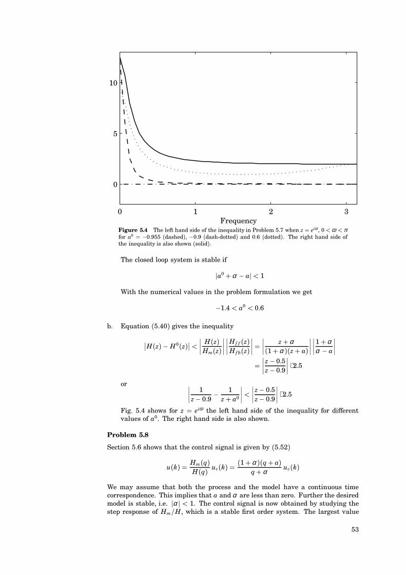
Fig. 5.4 shows for z eiω the left hand side of the inequality for differentvalues of a0. The right hand side is also shown.
Problem 5.8
Section 5.6 shows that the control signal is given by (5.52)
u(k) Hm(q)H(q) uc(k) (1+α )(q+ a)
q+α uc(k)
We may assume that both the process and the model have a continuous timecorrespondence. This implies that a and α are less than zero. Further the desiredmodel is stable, i.e. jα j < 1. The control signal is now obtained by studying thestep response of Hm/H, which is a stable first order system. The largest value
53
is then either at the first step or the final value. The magnitude at the first stepcan be determined either through the initial value theorem or by using seriesexpansion and the value is 1 + α . The final value is 1 + a. If jα j < jaj thenthe closed loop system is faster than the open loop system and the control signalis largest at the first step. If the desired response is slower than the open loopsystem then the final value is the largest one.
Problem 5.14
a. The rule of thumb on p. 130 gives
ωh 0.1 − 0.6
Identifying withs2 + 2ζ ω s +ω2
gives ω 0.1. Thus an appropriate sampling interval is
h 1 − 6
b. Using Example 2.16 we get sampled data characteristic equation
z2 + a1z+ a2 0
wherea1 −2e−ζ ω h cos(
√1 − ζ 2ωh) −1.32
a2 e−2ζ ω h 0.5
The poles are in 0.66 ± 0.25i.
Problem 5.15
This solution demonstrates how to use Algorithm 5.3.
Data: The process is given by A q2 − 1.6q + 0.65 and B 0.4q + 0.3. Acl
will at least contain Ac q2 − 0.7q + 0.25, other factors may be added lateron. Rd Sd 1 since no given factors are forced into the controller. Thedesired response to command signals is assumed to be Hm Bm/Am Bm/Ac 0.55/(q2− 0.7q+ 0.25) (cancelled process zero, Hm(1) 1).Pole excess condition:
deg Am − deg Bm ≥ deg A − deg B
2 − 0 ≥ 2 − 1
Remark: The fact that we cancel one zero and do not introduce any other zeroin Bm causes the delay from the command signal to be one time unit morethan the delay of the process.
Model following condition:
Bm B− Bm ⇒ Bm 0.55/0.4 1.375
Degree condition:
deg Acl 2 deg A+ deg Am + deg Rd + deg Sd − 1 2 ⋅ 2+ 2+ 0+ 0 − 1 5
with Acl A+B+Am Acl and Acl Ac Ao.
54
Step 1. A+ 1, A− A q2 − 1.6q+ 0.65, B+ q+ 0.75 and B− 0.4 achivescancellation of the process zero, but no cancellation of process poles.
Step 2. Using the degree condition above we may conclude that
deg Ao deg Acl − deg A+ − deg B+ − deg Am − deg Ac 5 − 0 − 1 − 2 − 2 0
The Diophantine equation to solve thus becomes
A−RdR + B−SdS Acl
(q2 − 1.6q+ 0.65)R + 0.4S q2 − 0.7q+ 0.25
Since this is of second order, R must be a constant, r0, say. In order to solve theidentity we must have two more parameters, so we let S s0q+ s1:
(q2 − 1.6q+ 0.65)r0+ (s0q+ s1) ⋅ 0.4 q2 − 0.7q+ 0.25
This gives the system of equations
r0 1
−1.6r0 + 0.4s0 −0.70.65r0 + 0.4s1 0.25
⇐⇒r0 1
s0 2.25
s1 −1
Step 3. The controller polynomials are now given by (5.45):R Am B+RdR Am(q+ 0.75)S Am A+SdS Am(2.25q− 1)T Bm A+ Acl 1.375 ⋅ Ac
Since, in this case, Am Ac, this factor can (and should) of course be cancelledin all controller polynomials, giving
R q+ 0.75
S 2.25q− 1
T 1.375
The corresponding degree of the closed-loop polynomial AR + B S will thus be 3instead of 5.
Problem 5.16
In this case we want to have an integrator in the controller, i.e., Rd (q−1). Thiswill increase the degree of the closed loop by one compared to Problem 5.15 (see(5.42)), which is done by having Ao (q+ ao), say. This gives the Diophantineequation
A−RdR + B−SdS Acl
(q2 − 1.6q+ 0.65)(q− 1)R + 0.4S (q2 − 0.7q+ 0.25)(q+ ao)R must still be a constant (which as usual will be 1) and S must be of secondorder:
(q2 − 1.6q+ 0.65)(q− 1) + (s0q2 + s1q+ s2) ⋅ 0.4 (q2 − 0.7q+ 0.25)(q+ a0)This gives
−2.6+ 0.4s0 a0 − 0.72.25+ 0.4s1 −0.7a0 + 0.25
−0.65+ 0.4s2 0.25a0
55
andS(q) 2.5
((a0 + 1.9)q2 − (0.7a0 + 2)q+ 0.25a0 + 0.65
)Using a0 −0.25, (5.45) gives (after cancelling the common factor Am):
R B+(q − 1) q2 − 0.25q− 0.75
S 4.125q2 − 4.5625q+ 1.46875
T Bm Ao 1.375q− 0.34375
Problem 5.17
The minimum degree solution has deg A0 1 and gives a unique solution to theDiophantine equation. Let us instead use deg A0 2 and deg S deg R−1. Thisgives the equation
(z+ 1)(z+ 2)(z2+ r1z+ r2) + z ⋅ (s1z+ s0) z2 ⋅ z2
with the solutionR0 z2 − 3z
S0 7z+ 6
The controller is causal. Using Theorem 5.1 we also have the solutions
R R0 + Qz
S S0 − Q(z− 1)(z− 2)
where Q is an arbitrary polynomial. Choose for instance Q −1. This gives
R z2 − 3z− z z2 − 4z
S 7z+ 6+ (z2 − 3z+ 2) z2 + 4z+ 8
This is also a causal controller. The closed loop systems when using R0A S0, T0 S0 and RA S, T S respectively are
B S0
AR0 + B S0 z(7z+ 6)
z4
B SAR + B S
z(z2 + 4z+ 8)z4
The number of zeros are different.
56
Solutions to Chapter 6
Problem 6.1
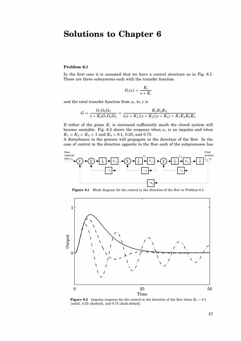
In the first case it is assumed that we have a control structure as in Fig. 6.1.There are three subsystems each with the transfer function
Gi(s) Ki
s+ Ki
and the total transfer function from uc to y is
G G1 G2G3
s+ K4G1 G2G3 K1K2 K3
s(s+ K1)(s+ K2)(s+ K3) + K1K2 K3K4
If either of the gains Ki is increased sufficiently much the closed system willbecome unstable. Fig. 6.2 shows the response when uc is an impulse and whenK1 K2 K3 1 and K4 0.1, 0.25, and 0.75.A disturbance in the process will propagate in the direction of the flow. In thecase of control in the direction opposite to the flow each of the subprocesses has
1sΣΣ K 1 Σ 2
1s
1
K4
Rawmaterialflow u c
Finalproductx =y
41s
K Σ
1
1s
K
1
3
x2 3x
−− −
−
Figure 6.1 Block diagram for the control in the direction of the flow in Problem 6.1.
0 25 50
0
1
Out
put
TimeFigure 6.2 Impulse response for the control in the direction of the flow when K4 0.1(solid), 0.25 (dashed), and 0.75 (dash-dotted).
57
1s
K 1Σ Σ 21s
1
K41s
K
1
1s
K
1
3
x3 2x
Σ
1s
u cx =y4
−− −
Figure 6.3 Block diagram for the control in the direction opposite of the flow in Problem 6.1.
a transfer function of the type Gi. The system is then represented with the blockdiagram in Fig. 6.3. Notice the order of the states. The system will remain stablefor all positive values of Ki. A disturbance will now propagate in the directionopposite the flow. A disturbance in uc will now only influence the first subprocessand will not propagate along with the flow. The reader is strongly recommended tocompare with the case where the disturbance appears at the final product storageinstead.
Problem 6.2
Fig. 6.3 in CCS contains several examples of couplings of simple control loops.
a. Cascade control loops are found for the cooling media flow and for the outputproduct flow.
b. Feedforward is used for the level control loop where the input flow is used asa measurable disturbance. The input flow is also used as feedforward for thecooling of the jacket.
c. Nonlinear elements are used in the flow control loops of the product outputand the coolant flow. The flow is probably measured using differential pres-sure which is proportional to the square of the flow. The square root deviceis thus used to remove the nonlinearity of the measurement device. An in-tentional nonlinearity is introduced in the selector. Either the temperatureor the pressure is used to control the coolant flow depending on the status ofthe process.
58
Solutions to Chapter 7
Problem 7.1
Which frequencies will the signal
f (t) a1 sin 2π t+ a2 sin 20t
give rise to when sampled with h 0.2?Since sampling is a linear operation we consider each component of f (t) separately.The sampled signal has the Fourier transform, see (7.3)
Fs 1h
∞∑k−∞
F(ω + kω s) ω s 2πh
where F(ω) is the Fourier transform of the time continuous signal. The Fouriertransform of sinω0t has its support (i.e., the set where it is 6 0) in the two points
±ω0. More precisely, it equals π i(
δ(
ω +ω0
)− δ
(ω −ω0
)). Thus, if the signal
sinω0 t is sampled with the sample interval h its Fourier transform will be 6 0 inthe points
±ω + kω s ; k 0A±1A±2A ( ( (For ω0 2π and ω s 2π/0.2 10π we get the angular frequencies
±2π ± k ⋅ 10π π(
±2A±8A±12A±18A±22A ( ( ()
ω 20 gives rise to
±20 ± k ⋅ 10π π(
±3.63A±6.37A±13.63A±16.37A ( ( ()
The output of the sampler is composed of the frequencies
π(
2A3.63A6.37A8A12A13.63A16.37A ( ( ()
Problem 7.2
We have the following specifications on the choice of sampling period and presam-pling filter:
1. All frequencies in the interval (− f1A f1) should be possible to reproduce fromthe samples of the continuous time signal.
2. We want to eliminate the disturbance with the known and fixed frequencyf2 5 f1.
The sampling theorem states that the first specification will be satisfied if andonly if the sample frequency fs is chosen such that
fs > 2 f1
Moreover, for the disturbance f2 not to fold on the data signal
( fs/2 − f1) > f2 − fs/2 ⇒ fs > f2 + f1 6 f1
Two cases:
59
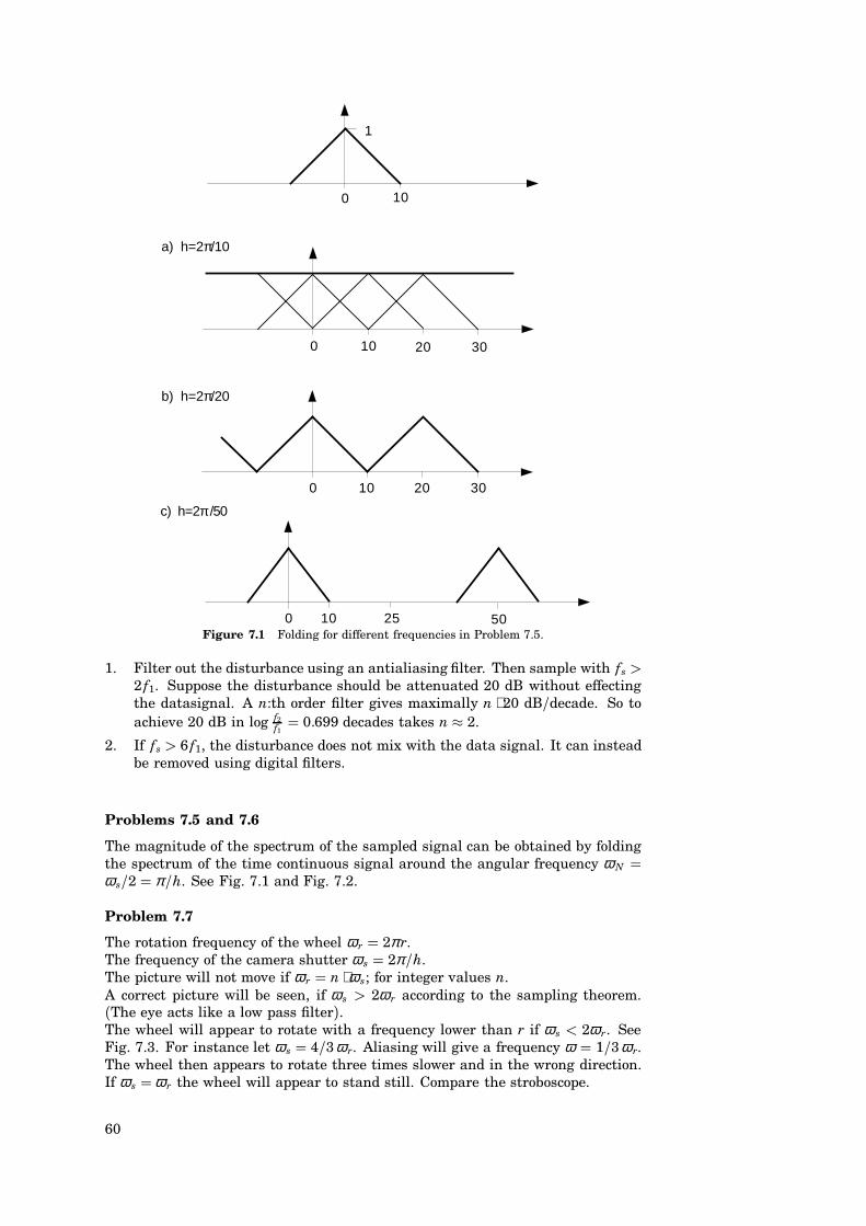
a) h=2π/10
1
10
b) h=2π/20
c) h=2π/50
0 10 20
10 25 50
0 10 20
0
0
30
30
Figure 7.1 Folding for different frequencies in Problem 7.5.
1. Filter out the disturbance using an antialiasing filter. Then sample with fs >2 f1. Suppose the disturbance should be attenuated 20 dB without effectingthe datasignal. A n:th order filter gives maximally n ⋅ 20 dB/decade. So toachieve 20 dB in log f2
f1 0.699 decades takes n 2.
2. If fs > 6 f1, the disturbance does not mix with the data signal. It can insteadbe removed using digital filters.
Problems 7.5 and 7.6
The magnitude of the spectrum of the sampled signal can be obtained by foldingthe spectrum of the time continuous signal around the angular frequency ω N ω s/2 π/h. See Fig. 7.1 and Fig. 7.2.
Problem 7.7
The rotation frequency of the wheel ω r 2π r.The frequency of the camera shutter ω s 2π/h.The picture will not move if ω r n ⋅ ω s; for integer values n.A correct picture will be seen, if ω s > 2ω r according to the sampling theorem.(The eye acts like a low pass filter).The wheel will appear to rotate with a frequency lower than r if ω s < 2ω r. SeeFig. 7.3. For instance let ω s 4/3ω r. Aliasing will give a frequency ω 1/3ω r.The wheel then appears to rotate three times slower and in the wrong direction.If ω s ω r the wheel will appear to stand still. Compare the stroboscope.
60
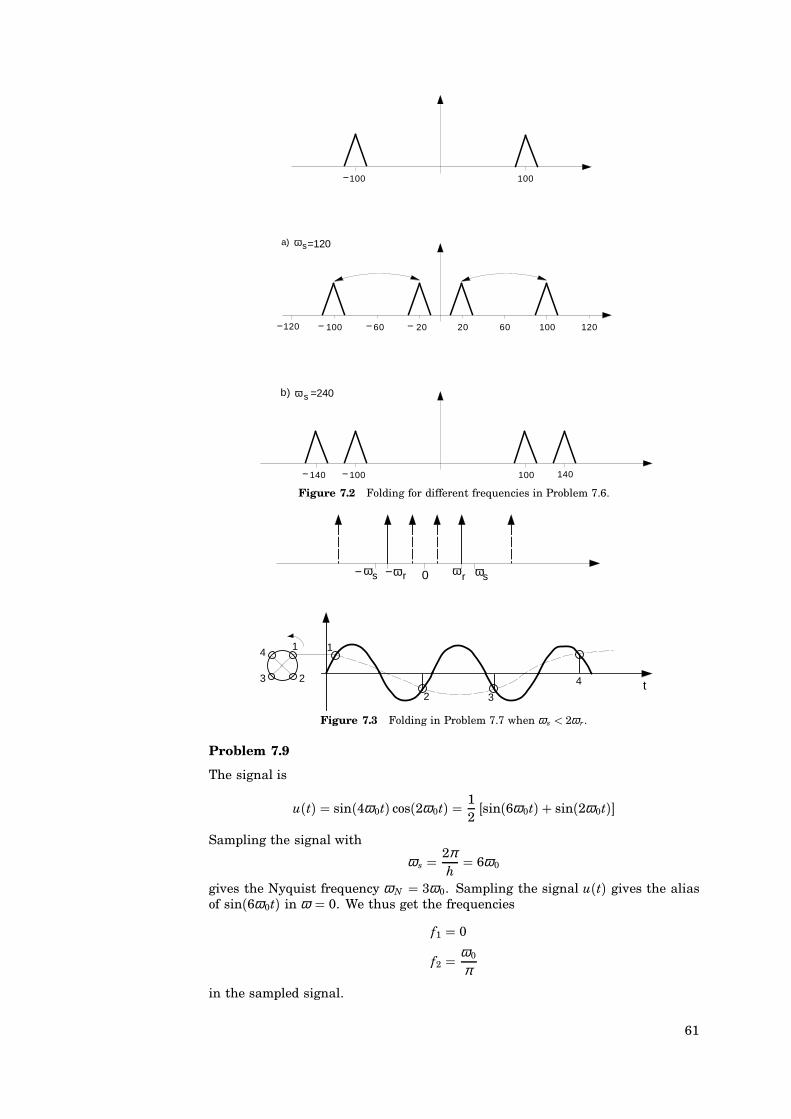
120 100 60 20 20 60 100 120
100
140 100 140100
100
a) ωs=120
ωsb) =240
−
−
−
−
−
−−
Figure 7.2 Folding for different frequencies in Problem 7.6.
ω ω ωωs r r s0
4
3 2
1 1
2 3
4 t
−−
Figure 7.3 Folding in Problem 7.7 when ω s < 2ω r.
Problem 7.9
The signal is
u(t) sin(4ω0t) cos(2ω0t) 12[sin(6ω0t) + sin(2ω0t)]
Sampling the signal with
ω s 2πh 6ω0
gives the Nyquist frequency ω N 3ω0. Sampling the signal u(t) gives the aliasof sin(6ω0t) in ω 0. We thus get the frequencies
f1 0
f2 ω0
π
in the sampled signal.
61
Solutions to Chapter 8
Problem 8.1
The three transformations Euler’s method (forward difference (8.4)), backwarddifference (8.5) and Tustin’s approximation (8.6) have different stability proper-ties. This can be seen by finding how the left half s-plane is transformed into thez-plane. For Euler’s method we have
z sh+ 1
This implies that the stability boundary in the sh-plane (the imaginary axis) istranslated one unit to the right, see Fig. 8.1a. When the backward difference isused then
z 11 − sh
For s iω we get1
1 −ωh
This represents a circle with radius 0.5 and going through the points 0 and 1, seeFig. 8.1b.Finally for Tustin’s approximation with s iω
z 1+ iωh/21− iωh/2
Nowjzj 1
arg z 2 arctanωh
The imaginary axis is thus transformed into the unit circle in the z-plane. If atransfer function is stable in the s-plane it will be translated into a stable discretetime system if using the backward difference or Tustin’s approximation.
Problem 8.2
G(s) as+ a
A a > 0
Forward differences Backward differences TustinFigure 8.1 Transformation of the left half s-plane when using a. Eulers method, b.Backward difference and c. Tustin’s approximation.
62
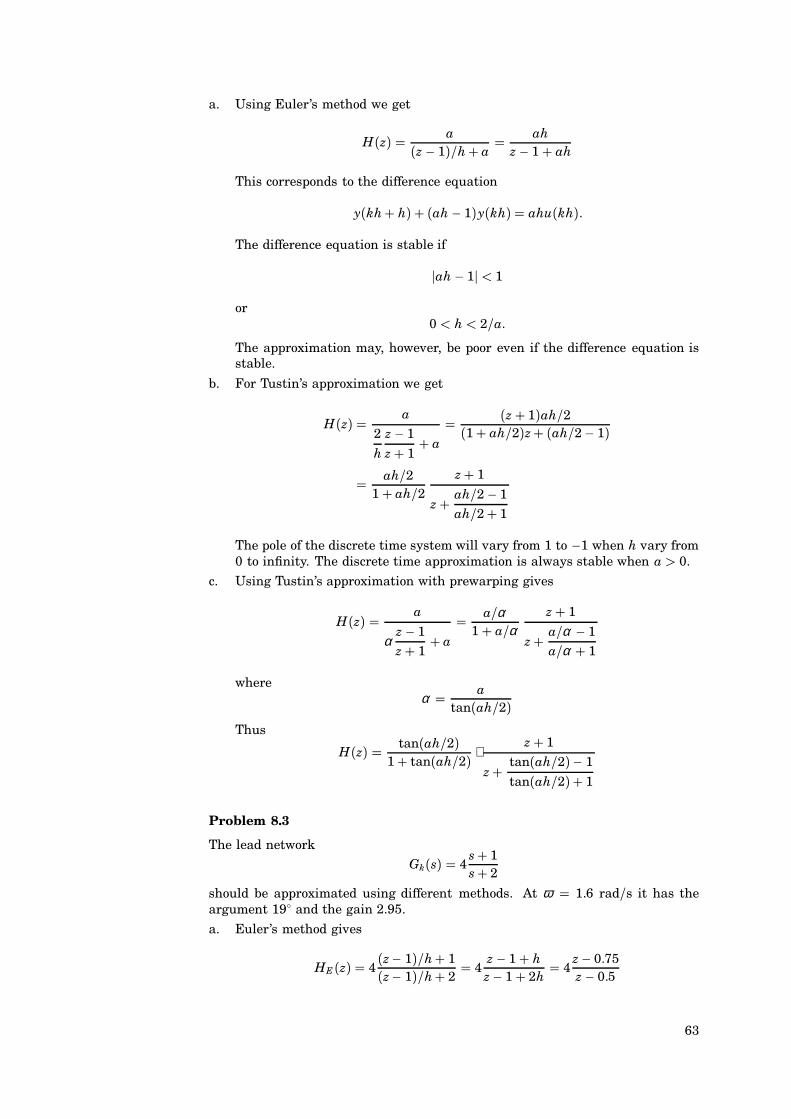
a. Using Euler’s method we get
H(z) a(z− 1)/h+ a
ahz− 1+ ah
This corresponds to the difference equation
y(kh+ h) + (ah− 1)y(kh) ahu(kh).
The difference equation is stable if
jah− 1j < 1
or0 < h < 2/a.
The approximation may, however, be poor even if the difference equation isstable.
b. For Tustin’s approximation we get
H(z) a2
h
z− 1
z+ 1+ a
(z+ 1)ah/2(1+ ah/2)z+ (ah/2− 1)
ah/21+ ah/2
z+ 1
z+ ah/2 − 1ah/2+ 1
The pole of the discrete time system will vary from 1 to −1 when h vary from0 to infinity. The discrete time approximation is always stable when a > 0.
c. Using Tustin’s approximation with prewarping gives
H(z) a
αz− 1z+ 1
+ a
a/α1+ a/α
z+ 1
z+ a/α − 1a/α + 1
whereα a
tan(ah/2)Thus
H(z) tan(ah/2)1+ tan(ah/2) ⋅
z+ 1
z+ tan(ah/2)− 1
tan(ah/2)+ 1
Problem 8.3
The lead networkGk(s) 4
s+ 1s+ 2
should be approximated using different methods. At ω 1.6 rad/s it has theargument 19 and the gain 2.95.
a. Euler’s method gives
HE(z) 4(z− 1)/h+ 1(z− 1)/h+ 2
4z− 1+ hz− 1+ 2h
4z− 0.75z− 0.5
63
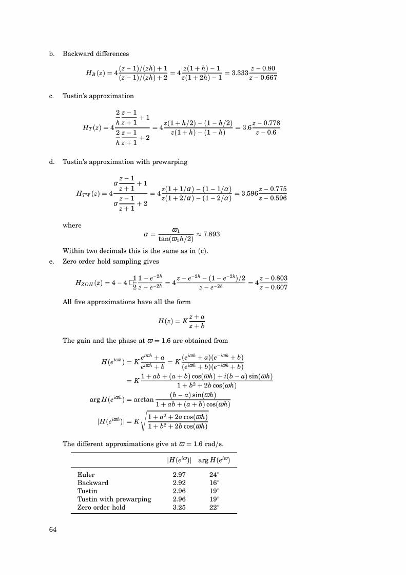
b. Backward differences
HB (z) 4(z− 1)/(zh)+ 1(z− 1)/(zh)+ 2
4z(1+ h) − 1z(1+ 2h)− 1
3.333z− 0.80z− 0.667
c. Tustin’s approximation
HT(z) 4
2h
z− 1z+ 1
+ 1
2h
z− 1z+ 1
+ 2
4z(1+ h/2)− (1 − h/2)
z(1+ h) − (1 − h) 3.6z− 0.778z− 0.6
d. Tustin’s approximation with prewarping
HTW (z) 4
αz− 1
z+ 1+ 1
αz− 1z+ 1
+ 2 4
z(1+ 1/α ) − (1 − 1/α )z(1+ 2/α ) − (1 − 2/α ) 3.596
z− 0.775z− 0.596
whereα ω1
tan(ω1h/2) 7.893
Within two decimals this is the same as in (c).e. Zero order hold sampling gives
HZOH (z) 4 − 4 ⋅12
1 − e−2h
z− e−2h 4z− e−2h − (1− e−2h)/2
z− e−2h 4z− 0.803z− 0.607
All five approximations have all the form
H(z) Kz+ az+ b
The gain and the phase at ω 1.6 are obtained from
H(eiω h) Keiω h + aeiω h + b
K(eiω h + a)(e−iω h + b)(eiω h + b)(e−iω h+ b)
K1+ ab+ (a+ b) cos(ωh) + i(b− a) sin(ωh)
1+ b2 + 2b cos(ωh)arg H(eiω h) arctan
(b− a) sin(ωh)1+ ab+ (a+ b) cos(ωh)
jH(eiω h)j K
√1+ a2 + 2a cos(ωh)1+ b2 + 2b cos(ωh)
The different approximations give at ω 1.6 rad/s.
jH(eiω )j arg H(eiω)Euler 2.97 24
Backward 2.92 16
Tustin 2.96 19
Tustin with prewarping 2.96 19
Zero order hold 3.25 22
64
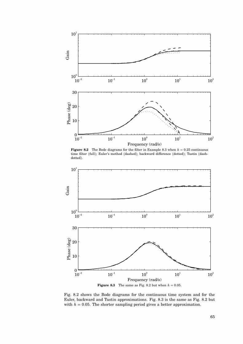
10−2 10−1 100 101 102100
101
Gai
n
10−2 10−1 100 101 1020
10
20
30
Pha
se (d
eg)
Frequency (rad/s)Figure 8.2 The Bode diagrams for the filter in Example 8.3 when h 0.25 continuoustime filter (full); Euler’s method (dashed); backward difference (dotted); Tustin (dash-dotted).
10−2 10−1 100 101 102100
101
Gai
n
10−2 10−1 100 101 1020
10
20
30
Pha
se (d
eg)
Frequency (rad/s)Figure 8.3 The same as Fig. 8.2 but when h 0.05.
Fig. 8.2 shows the Bode diagrams for the continuous time system and for theEuler, backward and Tustin approximations. Fig. 8.3 is the same as Fig. 8.2 butwith h 0.05. The shorter sampling period gives a better approximation.
65
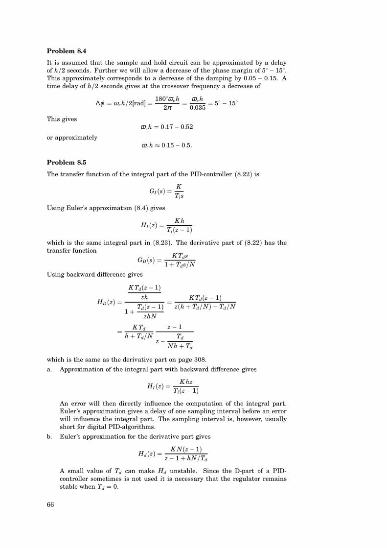
Problem 8.4
It is assumed that the sample and hold circuit can be approximated by a delayof h/2 seconds. Further we will allow a decrease of the phase margin of 5 − 15 .This approximately corresponds to a decrease of the damping by 0.05 − 0.15. Atime delay of h/2 seconds gives at the crossover frequency a decrease of
∆ϕ ω ch/2[rad] 180 ω ch2π ω ch
0.035 5 − 15
This givesω ch 0.17− 0.52
or approximatelyω ch 0.15− 0.5.
Problem 8.5
The transfer function of the integral part of the PID-controller (8.22) is
GI (s) KTis
Using Euler’s approximation (8.4) gives
HI(z) K hTi(z− 1)
which is the same integral part in (8.23). The derivative part of (8.22) has thetransfer function
GD(s) K Tds1+ Tds/N
Using backward difference gives
HD(z)
K Td(z− 1)zh
1+ Td(z− 1)zhN
K Td(z− 1)z(h+ Td/N) − Td/N
K Td
h+ Td/Nz− 1
z−Td
Nh + Td
which is the same as the derivative part on page 308.
a. Approximation of the integral part with backward difference gives
HI (z) K hzTi(z− 1)
An error will then directly influence the computation of the integral part.Euler’s approximation gives a delay of one sampling interval before an errorwill influence the integral part. The sampling interval is, however, usuallyshort for digital PID-algorithms.
b. Euler’s approximation for the derivative part gives
Hd(z) K N(z− 1)z− 1+ hN/Td
A small value of Td can make Hd unstable. Since the D-part of a PID-controller sometimes is not used it is necessary that the regulator remainsstable when Td 0.
66
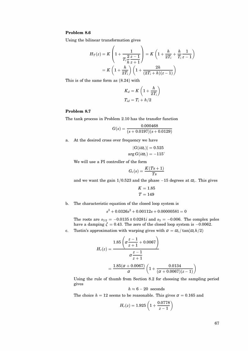
Problem 8.6
Using the bilinear transformation gives
HT (z) K
1+ 1
Ti2h
z− 1z+ 1
K(
1+ h2Ti
+ hTi
1z− 1
)
K(
1+ h2Ti
)(1+ 2h
(2Ti+ h)(z− 1))
This is of the same form as (8.24) with
Kd K(
1+ h2Ti
)Tid Ti + h/2
Problem 8.7
The tank process in Problem 2.10 has the transfer function
G(s) 0.000468(s+ 0.0197)(s+ 0.0129)
a. At the desired cross over frequency we have
jG(iω c)j 0.525
arg G(iω c) −115
We will use a PI controller of the form
Gr(s) K (Ts+ 1)Ts
and we want the gain 1/0.523 and the phase −15 degrees at ω c. This gives
K 1.85
T 149
b. The characteristic equation of the closed loop system is
s3 + 0.0326s2+ 0.00112s+ 0.00000581 0
The roots are s1A2 −0.0135 ± 0.0281i and s3 −0.006. The complex poleshave a damping ζ 0.43. The zero of the closed loop system is −0.0062.
c. Tustin’s approximation with warping gives with α ω c/ tan(ω ch/2)
Hr(z) 1.85
(α
z− 1z+ 1
+ 0.0067
)
αz− 1
z+ 1
1.85(α + 0.0067)α
(1+ 0.0134
(α + 0.0067)(z− 1))
Using the rule of thumb from Section 8.2 for choosing the sampling periodgives
h 6− 20 seconds
The choice h 12 seems to be reasonable. This gives α 0.165 and
Hr(z) 1.925(
1+ 0.0778z− 1
)
67
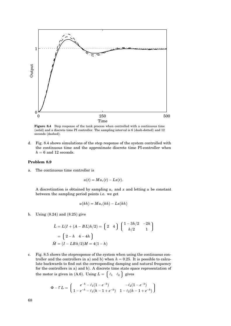
0 250 5000
1
Ou
tpu
t
TimeFigure 8.4 Step response of the tank process when controlled with a continuous time(solid) and a discrete time PI controller. The sampling interval is 6 (dash-dotted) and 12seconds (dashed).
d. Fig. 8.4 shows simulations of the step response of the system controlled withthe continuous time and the approximate discrete time PI-controller whenh 6 and 12 seconds.
Problem 8.9
a. The continuous time controller is
u(t) Muc(t)− Lx(t).
A discretization is obtained by sampling uc and x and letting u be constantbetween the sampling period points i.e. we get
u(kh) Muc(kh)− Lx(kh)
b. Using (8.24) and (8.25) give
L L(I + (A− B L)h/2) 2 4
1 − 3h/2 −2h
h/2 1
2− h 4 − 4h
M (I − LBh/2)M 4(1− h)
c. Fig. 8.5 shows the stepresponse of the system when using the continuous con-troller and the controllers in a) and b) when h 0.25. It is possible to calcu-late backwards to find out the corresponding damping and natural frequencyfor the controllers in a) and b). A discrete time state space representation of
the motor is given in (A.6). Using L X1 X2
gives
Φ − ΓL e−h − X1(1 − e−h) −X2(1− e−h)
1− e−h − X1(h− 1+ e−h) 1 − X2(h− 1+ e−h)
68
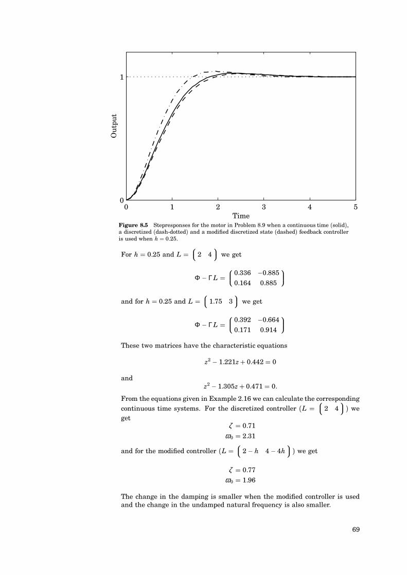
0 1 2 3 4 50
1
Ou
tpu
t
TimeFigure 8.5 Stepresponses for the motor in Problem 8.9 when a continuous time (solid),a discretized (dash-dotted) and a modified discretized state (dashed) feedback controlleris used when h 0.25.
For h 0.25 and L 2 4
we get
Φ − ΓL 0.336 −0.885
0.164 0.885
and for h 0.25 and L
1.75 3 we get
Φ − ΓL 0.392 −0.664
0.171 0.914
These two matrices have the characteristic equations
z2 − 1.221z+ 0.442 0
andz2 − 1.305z+ 0.471 0.
From the equations given in Example 2.16 we can calculate the correspondingcontinuous time systems. For the discretized controller (L
2 4) we
getζ 0.71
ω0 2.31
and for the modified controller (L 2 − h 4 − 4h
) we get
ζ 0.77
ω0 1.96
The change in the damping is smaller when the modified controller is usedand the change in the undamped natural frequency is also smaller.
69
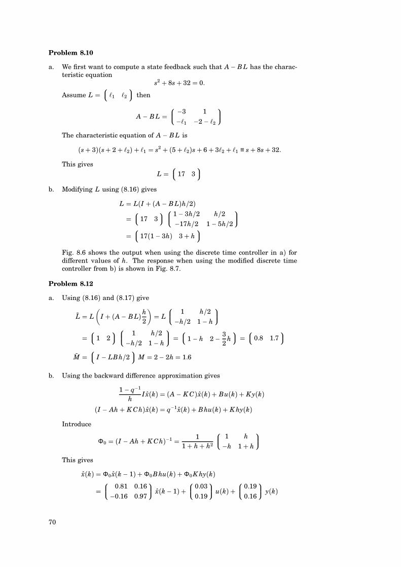
Problem 8.10
a. We first want to compute a state feedback such that A− B L has the charac-teristic equation
s2 + 8s+ 32 0.
Assume L X1 X2
then
A − B L −3 1
−X1 −2 − X2
The characteristic equation of A − B L is
(s+ 3)(s+ 2+ X2) + X1 s2 + (5+ X2)s+ 6+ 3X2 + X1 ≡ s+ 8s+ 32.
This givesL
17 3
b. Modifying L using (8.16) gives
L L(I + (A − B L)h/2)
17 3
1 − 3h/2 h/2−17h/2 1 − 5h/2
17(1− 3h) 3+ h
Fig. 8.6 shows the output when using the discrete time controller in a) fordifferent values of h. The response when using the modified discrete timecontroller from b) is shown in Fig. 8.7.
Problem 8.12
a. Using (8.16) and (8.17) give
L L(
I + (A− B L)h2
) L
1 h/2−h/2 1 − h
1 2
1 h/2−h/2 1 − h
1 − h 2 − 32
h 0.8 1.7
M
I − LBh/2M 2− 2h 1.6
b. Using the backward difference approximation gives
1 − q−1
hIx(k) (A − K C)x(k)+ Bu(k) + K y(k)
(I − Ah+ K Ch)x(k) q−1 x(k) + Bhu(k) + K hy(k)Introduce
Φ0 (I − Ah + K Ch)−1 11+ h+ h2
1 h
−h 1+ h
This gives
x(k) Φ0 x(k− 1) + Φ0 Bhu(k) + Φ0 K hy(k)
0.81 0.16
−0.16 0.97
x(k− 1) + 0.03
0.19
u(k) + 0.19
0.16
y(k)
70
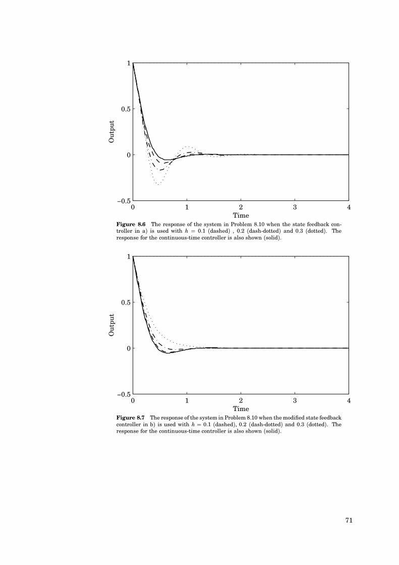
0 1 2 3 4−0.5
0
0.5
1
Out
put
TimeFigure 8.6 The response of the system in Problem 8.10 when the state feedback con-troller in a) is used with h 0.1 (dashed) , 0.2 (dash-dotted) and 0.3 (dotted). Theresponse for the continuous-time controller is also shown (solid).
0 1 2 3 4−0.5
0
0.5
1
Out
put
TimeFigure 8.7 The response of the system in Problem 8.10 when the modified state feedbackcontroller in b) is used with h 0.1 (dashed), 0.2 (dash-dotted) and 0.3 (dotted). Theresponse for the continuous-time controller is also shown (solid).
71
Solutions to Chapter 10
Problem 10.1
a. Better sensors, for instance a tachometer with less noise.
b. Flow control with local feedback.
c. Temperature control in houses.
Problem 10.2
a. The time function y(t) sin(ω t) has the z-transform
Y(z) z sinωhz2 − 2z cosωh+ 1
See Table 2.1. Consider a system with
Hd(z) Y(z)
The impulse response of Hd will thus be sin(khω). That this is the correctanswer is easily seen by making long division.
Hd(z) sin(hω)z−1+ sin(2hω)z−2+ sin(3hω)z−3+ ⋅ ⋅ ⋅
b. The time function t ⋅ e−t has the z-transform
Y(z) he−hz(z− e−h)2
This can be found by looking in a table of z-transforms. The desired systemthus has the z-transform
Hd(z) he−hz(z− e−h)2
Long division gives
Hd(z) he−hz−1 + 2he−2hz−2 + ⋅ ⋅ ⋅
Problem 10.3
Using the model of the disturbance gives
y(k+m) C(q)A(q)w(k+m).
Introduce the identity
qm−1C(q) A(q)F(q)+ G(q)
where deg F m − 1 and deg G n− 1. Then
y(k+m) F(q)w(k+ 1) + qG(q)A(q) w(k) F(q)w(k+ 1) + qG(q)
C(q) y(k)
72
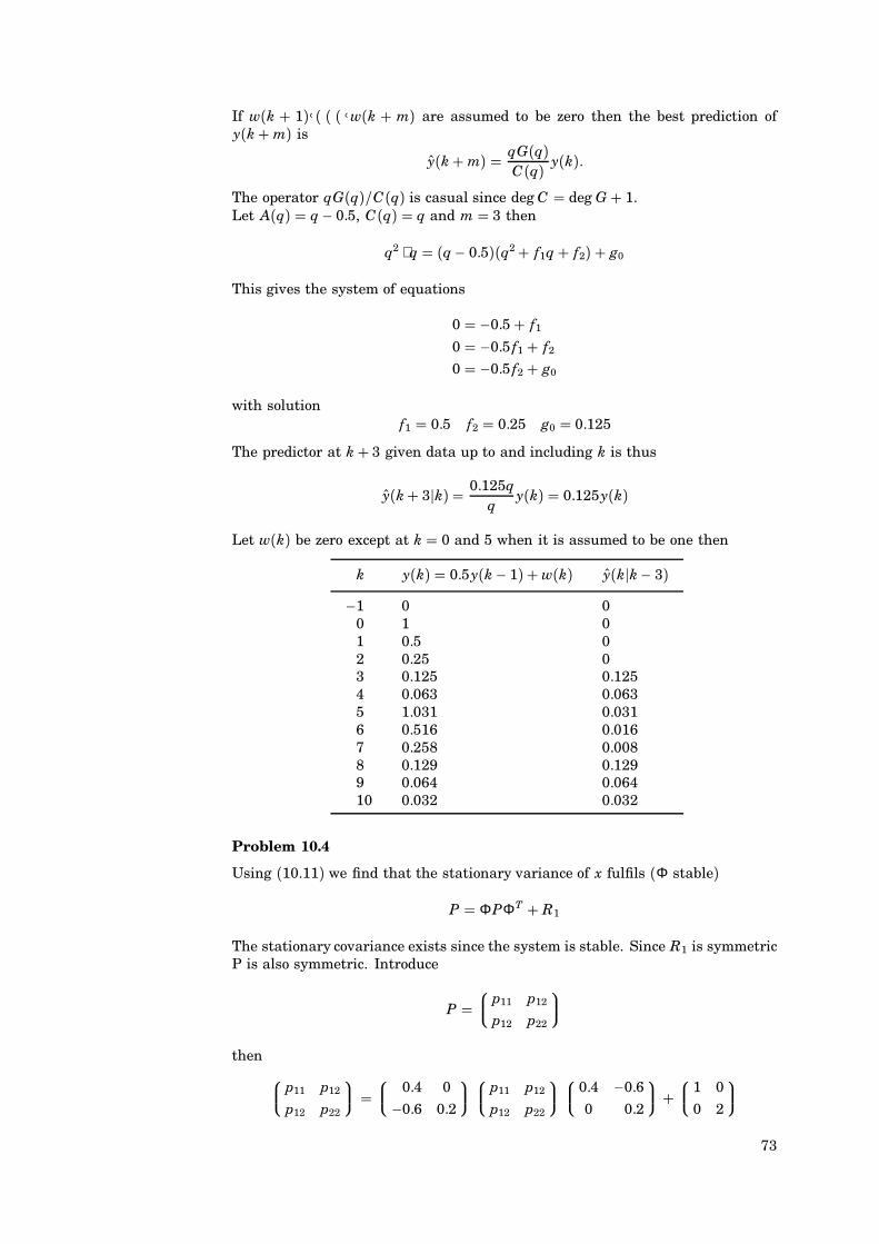
If w(k + 1)A ( ( ( Aw(k + m) are assumed to be zero then the best prediction ofy(k+m) is
y(k+m) qG(q)C(q) y(k).
The operator qG(q)/C(q) is casual since deg C deg G + 1.Let A(q) q− 0.5, C(q) q and m 3 then
q2 ⋅ q (q− 0.5)(q2+ f1q+ f2) + g0
This gives the system of equations
0 −0.5+ f1
0 −0.5 f1 + f2
0 −0.5 f2 + g0
with solutionf1 0.5 f2 0.25 g0 0.125
The predictor at k+ 3 given data up to and including k is thus
y(k+ 3jk) 0.125qq
y(k) 0.125y(k)
Let w(k) be zero except at k 0 and 5 when it is assumed to be one then
k y(k) 0.5y(k− 1) + w(k) y(kjk− 3)−1 0 0
0 1 01 0.5 02 0.25 03 0.125 0.1254 0.063 0.0635 1.031 0.0316 0.516 0.0167 0.258 0.0088 0.129 0.1299 0.064 0.06410 0.032 0.032
Problem 10.4
Using (10.11) we find that the stationary variance of x fulfils (Φ stable)
P ΦPΦT + R1
The stationary covariance exists since the system is stable. Since R1 is symmetricP is also symmetric. Introduce
P p11 p12
p12 p22
then p11 p12
p12 p22
0.4 0
−0.6 0.2
p11 p12
p12 p22
0.4 −0.60 0.2
+ 1 0
0 2
73
This givesp11 0.16p11 + 1
p12 −0.24p11 + 0.08p12
p22 0.36p11 − 0.24p12 + 0.04p22 + 2
The solution is
P 1.19 −0.31
−0.31 2.61
The stationary covariance function is
Ex(k+ τ )x(k)T Φτ P
It remains to compute Φτ . The eigenvalues of Φ are λ 1 0.4 and λ 2 0.2. Usingthe results on matrix functions in Appendix B we get
Φτ α 0I +α 1Φ
where α 0 and α 1 are obtained from
λτ1 α 0 +α 1λ 1
λτ2 α 0 +α 1λ 2
The solution is
α 0 −λ 1λ 2(λτ−11 − λτ−1
2 )λ 1 − λ 2
α 1 λτ1 − λτ
2
λ 1 − λ 2
and
Φτ 0.4τ 0
−3(0.4τ − 0.2τ ) 0.2τ
Finally
rx(τ ) 1.19 ⋅ 0.4τ −0.31 ⋅ 0.4τ
−3.57 ⋅ 0.4τ + 3.27 ⋅ 0.2τ 0.93 ⋅ 0.4τ + 1.68 ⋅ 0.2τ
τ ≥ 0
Problem 10.5
From the state space description we get the input-output description of the process
y(k) + a1 y(k− 1) + ⋅ ⋅ ⋅ + an y(k− n) c1v(k − 1) + ⋅ ⋅ ⋅+ cnv(k − n)
where aiA i 1A ( ( ( A n are the coefficients of the characteristic polynomial ofthe matrix Φ. Multiply the equation above by y(k−τ ) and take the mathematicalexpectation. y(k−τ ) is independent of all the terms on the right hand if τ > n+1.Thus
ry(τ ) + a1ry(τ − 1) + ⋅ ⋅ ⋅+ anry(τ − n) 0.
This is called the Yule-Walker equation.
Problem 10.6
There are two noise sources v1 and v2 that is used to generate y(k). Using Theorem10.2 we find that the spectral density of y is
φ y H(z)φ vHT(z−1)
74
where z eiω
H(z) C(zI − Φ)−1Γ 1 1
z+ a 0
0 z+ b
−1
1 1
z+a1
z+b
and
φ v σ 2
1 0
0 σ 22
Thus
φ y 1
z+a1
z+b
σ 21 0
0 σ 22
1z−1+a
1z−1+b
σ 2
1
(z+ a)(z−1+ a) +σ 2
2
(z+ b)(z−1+ b)
σ 21 (z+ b)(z−1+ b) + σ 2
2(z+ a)(z−1+ a)(z+ a)(z+ b)(z−1+ a)(z−1+ b)
Using the spectral factorization theorem (Theorem 10.3) we find that we cangenerate the same spectral density by sending white noise through
H1(z) λ z+ c(z+ a)(z+ b)
this gives the spectral density
φ 1 λ 2 (z+ c)(z−1+ c)(z+ a)(z−1+ a)(z+ b)(z−1+ b)
Identification with φ y gives the relationship
λ 2(1+ c2) σ 21 (1+ b2) + σ 2
2(1+ a2)λ 2c σ 2
1 b+ σ 2a
Problem 10.7
The process isx(k+ 1) ax(k) + v(k)
y(k) x(k) + e(k)This is the same as in Example 10.3 with the exception that Ev(k)e(s) r12δ (k−s). The covariance function for x will thus be the same but the covariance of y willcontain an additional term due to the correlation between v and e. From Example10.3 we know that
rx(τ ) ajτ jr1
1 − a2
The covariance of y is
ry(τ ) E y(k+ τ )y(k) E [x(k+ τ ) + e(k+ τ )] [x(k) + e(k)] rx(τ ) + rxe(τ ) + rex(τ ) + re(τ ) rx(τ ) + rxe(τ ) + rxe(−τ ) + re(τ )
where it has been used that rex(τ ) rxe(−τ ) in stationarity.
rxe(τ + 1) E x(k+ τ + 1)e(k) E [ax(k+ τ ) + v(k+ τ )] e(k) arxe(τ ) + rve(τ )
75
The last term is zero except for τ 0, where it is r12. The first term is zero forτ ≤ 0. It is natural that white noise in the future is uncorrelated with the presentvalue of x. This gives
rxe(τ )
0 τ ≤ 0
r12 τ 1
aτ−1r12 τ > 1
0 τ ≤ 0
aτ−1r12 τ ≥ 1
and
ry(τ )
a−τ r1
1−a2 + 0+ a−τ−1r12 + 0 τ < 0r1
1−a2 + 0+ 0+ r2 τ 0
aτ r11−a2 + aτ−1r12 + 0+ 0 τ > 0
ajτ j r11−a2 + ajτ j−1r12 τ 6 0
r11−a2 + r2 τ 0
The definition of spectral density gives
φ y(ω) 12π
∞∑τ−∞
ry(τ )e−iωτ
12π
[ r1
1− a2 −r12
a
] 1− a2
(eiω − a)(e−iω − a) −r1
1− a2 −r12
a+ r1
1− a2 + r2
12π
r1a+ r12(1− a2) − r12(eiω − a)(e−iω − a) + r2a(eiω − a)(e−iω − a)a(eiω − a)(e−iω − a)
(1)
where it has been used that
∞∑τ−∞
ajτ je−iωτ 1 − a2
(eiω − a)(e−iω − a)
The spectral density for
y(k) λ q − cq − a
ε (k)
is (see Theorem 10.2)
φ y(ω) λ 2
2π(eiω − c)(e−iω − c)(eiω − a)(e−iω − a) (2)
Identification of (1) with (2) gives the relationr1 + r121 − a2
a− r12
1+ a2
a+ r2a
1+ a2
a λ 2(1+ c2)
r12 − r2a −λ 2c
⇔r2(1+ a2) + r1 − 2ar12 λ 2(1+ c2)r2a − r12 λ 2c
A more elegant solution The ouput can be written as
y(k) H(q) 1
v(k)e(k)
76
where H(z) 1z−a . The spectral density of y is given by
φ y 12π
H(z) 1 r1 r12
r12 r2
H(z−1)1
1
2πr1 H(z)H(z−1) + r12 H(z) + r12 H(z−1) + r2
12π
r1
(z− a)(z−1 − a) + r12
(1
z− a+ 1
z−1 − a
)+ r2
12π
z(r12 − r2a) + r1 − 2ar12 + r2(1+ a2) + z−1(r12 − r2a)(z− a)(z−1 − a)
which gives the same equations as in the previous methodr2(1+ a2) + r1 − 2ar12 λ 2(1+ c2)
ar2 − r12 λ 2c
Problem 10.8
The process can be written as
y(k) q − cq− a
e(k) a− cq− a
e(k)+ e(k) x(k) + e(k)
wherex(k+ 1) ax(k) + (a− c)e(k)
Using Problem 10.7 we find that
r1 (a− c)2r12 a− c
r2 1
Thus
ry(τ ) ajτ jr1
1 − a2 + ajτ j−1r12
with a 0.7 and c 0.5 we get for τ 6 0
ry(τ ) (0.7)jτ j 0.041 − 0.49
+ 0.20.7(0.7)jτ j 0.36(0.7)jτ j
For τ 0
ry(0) r1
1− a2 + r2 (a− c)21 − a2 + 1 1.08
The variance can also be obtained from Theorem 10.4.
ry(0) I1 1+ c2 − 2ac1 − a2 1.08
Further (10.17) gives
φ y 12π(z− c)(z−1 − c)(z− a)(z−1 − a) )
12π
1.25− cosω1.49− 1.4 cosω
where z eiω .
77
Problem 10.9
The variance of the process
y(k) q2 + 0.2qq2 − 1.5q+ 0.7
e(k) b0q2 + b1q+ b2
a0q2 + a1q+ a2e(k)
can be determined using Theorem 10.4. The formula for I2 gives
B0 1+ (0.2)2+ 0 1.04
B1 2(0.2+ 0) 0.4B2 0
e1 1.7
and
ry(0) I2 1.04 ⋅ 1.7+ 0.4 ⋅ 1.5(1 − 0.49)1.7− 1.5 ⋅ 1.5(1− 0.7) 12.33
The recursive scheme in Section 10.4 can also be used to get
1 −1.5 0.7 1 0.2 0
0.7 −1.5 1 α 2 0.7 0.7 −1.5 1 β 2 0
0.51 −0.45 1 0.2
−0.45 0.51 α 1 −0.8824 −0.45 0.51 β 1 0.3922
0.1129 1.1765
0.1129 β 0 10.4167
This givesI2 10.4167 ⋅ 1.1765+ 0.3922 ⋅ 0.2 12.33
These calculations have been performed in high precision and thereafter round-ed.
Problem 10.10
The process is
y(k) e(k)− 2e(k− 1) + 3e(k− 2)− 4e(k− 3)ry(τ ) Ey(k+ τ )y(k)
This gives
ry(0) E(e(k)− 2e(k− 1) + 3e(k− 2) − 4e(k− 3))2
E
e(k)2+ 4e(k− 1)2 + 9e(k− 2)2 + 16e(6− 3)2 + crossterms
1+ 4+ 9+ 16 30
The mean value of the crossterms are zero since
E e(k+ τ )e(k) 0 τ 6 0
In the same way
ry(1) 1 ⋅ (−2) + (−2) ⋅ 3+ 3 ⋅ (−4) −20
ry(2) 1 ⋅ 3+ (−2) ⋅ (−4) 11
ry(3) 1 ⋅ (−4) −4
ry(4) 0 k ≥ 4
78
Problem 10.11
Φ y 11.36+ 1.2 cosω
a.
H(z) bz− a
Using Theorem 10.2 we get
φ y(ω) H(eiω )φ u(ω)H(e−iω) H(eiω ) 12π H(e−iω )
1
2π b2(eiω − a
)(e−iω − a
) b2/2π
1+ a2 − a ⋅ 2(eiω + e−iω
2
) b2/2π
1+ a2 − 2a cosω 1
2π 1+ a2
b2 − 2π 2a−b2 cosω
Identifying with the desired spectral density gives
2π (1+ a2) b2 ⋅ 1.36
2π (2a) −1.2b2
Divide the two equations
1+ a2
2a −1.36
1.2⇒ a2 + 2.72
1.2a+ 1 0
a −1.361.2
±√(1.36
1.2
)2− 1 −0.6
b √
2a−1.2
⋅ 2π √
2π
The desired filter is
H(z) √
2πz+ 0.6
b. Theorem 10.4 CCS Var y I1 2π1− 0.62
2π0.64
Problem 10.12
x(k+ 1) 0.3 0.2
0 0.5
x(k) + 0
1
u(k) + v(k)
The stationary covariance is given by
P ΦPΦT + R1 p11 p12
p12 p22
0.3 0.20 0.5
p11 p12
p12 p22
0.3 0
0.2 0.5
+ 1 0
0 0.5
p11 0.09p11 + 0.12p12 + 0.04p22 + 1
p12 0.15p12 + 0.1p22
p22 0.25p22 + 0.5
P 1.1385 0.0784
0.0784 0.667
79

Problem 10.13
Example 10.4 shows that the filter
H(z) bz− a
gives the spectral density
Φ(ω) r1
2π ⋅b2
1+ a2 − 2a cosω
In this case r1 1. Identify with the desired spectral density gives
12π
⋅3
5.43− 5.40 cosω 1
2π1
1.81− 1.8 cosω
This gives a 0.9 and b 1.
80
Solutions to Chapter 11
Problem 11.1
For the system we have
ddt
Φ(tA kh) −aΦ(tA kh)A Φ(khA kh) 1
This differential equation has the solution
Φ(tA kh) e−a(t−kh)
and
Γ(tA kh) t∫
kh
e−a(t−s)b ds ba(1− e−a(t−kh))
The discrete time loss function is obtained from CCS (11.6)-(11.8), which gives
Q1 ∫ kh+h
khe−2a(s−kh)ds 1
2a(1 − e−2ah)
Q12 ∫ kh+h
khe−a(s−kh)b
a(1− e−a(s−kh)) ds b
2a2 (1 − e−ah)2
Q2 ∫ kh+h
kh
(b2
a2 (1 − e−a(s−kh))2 + ρ)
ds
(
b2
a2 + ρ)
h− b2
2a3
(3 − 4e−ah+ e−2ah
)
Notice that there will be a Q12 term even if Q12c 0.
Problem 11.2
x 0 1
0 0
x+ 0
1
u
y 1 0
x
Sample the system
Φ eAh 1 h
0 1
Γ
h∫0
eAτ B dτ h2/2
h
81
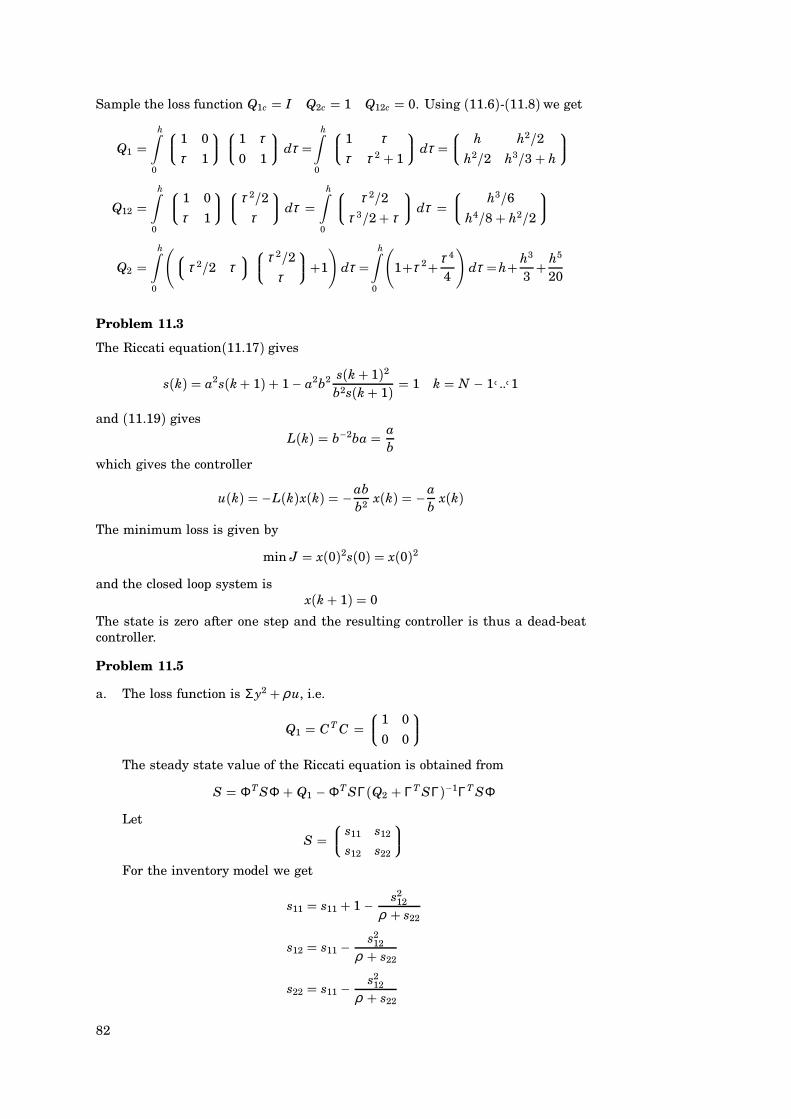
Sample the loss function Q1c I Q2c 1 Q12c 0. Using (11.6)-(11.8)we get
Q1 h∫
0
1 0
τ 1
1 τ0 1
dτ h∫
0
1 ττ τ 2 + 1
dτ h h2/2
h2/2 h3/3+ h
Q12
h∫0
1 0
τ 1
τ 2/2τ
dτ h∫
0
τ 2/2τ 3/2+ τ
dτ h3/6
h4/8+ h2/2
Q2
h∫0
(τ 2/2 ττ 2/2
τ
+1
)dτ
h∫0
(1+τ 2+ τ 4
4
)dτ h+ h3
3+ h5
20
Problem 11.3
The Riccati equation(11.17) gives
s(k) a2s(k+ 1) + 1− a2b2 s(k+ 1)2b2s(k+ 1) 1 k N − 1A ..A1
and (11.19) gives
L(k) b−2ba ab
which gives the controller
u(k) −L(k)x(k) −abb2 x(k) −a
bx(k)
The minimum loss is given by
min J x(0)2s(0) x(0)2
and the closed loop system isx(k+ 1) 0
The state is zero after one step and the resulting controller is thus a dead-beatcontroller.
Problem 11.5
a. The loss function is Σ y2 + ρ u, i.e.
Q1 CT C 1 0
0 0
The steady state value of the Riccati equation is obtained from
S ΦT SΦ + Q1 − ΦT SΓ(Q2 + ΓT SΓ)−1ΓT SΦ
Let
S s11 s12
s12 s22
For the inventory model we get
s11 s11 + 1 − s212
ρ + s22
s12 s11 −s2
12
ρ + s22
s22 s11 −s2
12
ρ + s22
82
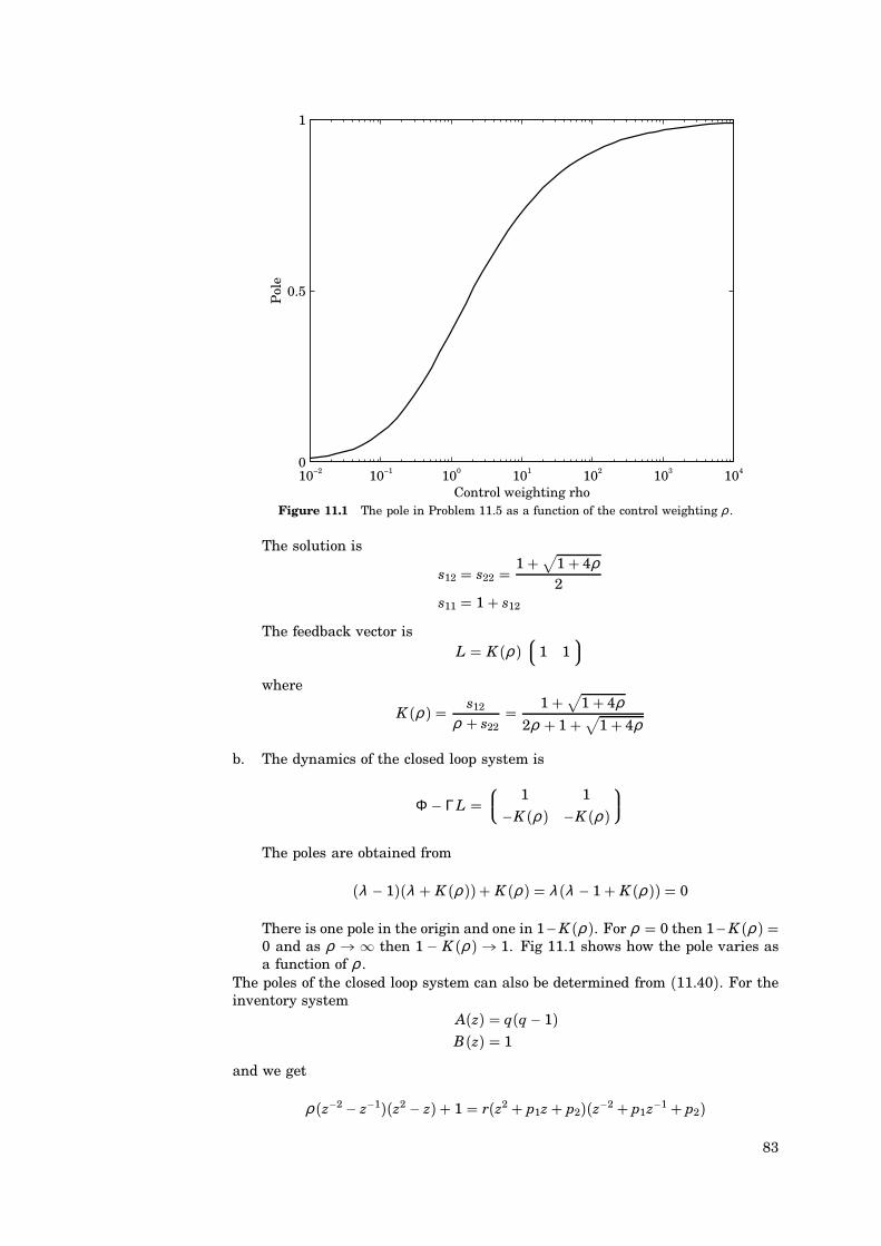
10−2 10−1 100 101 102 103 1040
0.5
1
Pol
e
Control weighting rhoFigure 11.1 The pole in Problem 11.5 as a function of the control weighting ρ .
The solution is
s12 s22 1+√1+ 4ρ2
s11 1+ s12
The feedback vector isL K (ρ )
1 1
where
K (ρ ) s12
ρ + s22 1+√1+ 4ρ
2ρ + 1+√1+ 4ρ
b. The dynamics of the closed loop system is
Φ − ΓL 1 1
−K (ρ ) −K (ρ )
The poles are obtained from
(λ − 1)(λ + K (ρ ))+ K (ρ ) λ (λ − 1+ K (ρ )) 0
There is one pole in the origin and one in 1−K (ρ ). For ρ 0 then 1−K (ρ ) 0 and as ρ → ∞ then 1 − K (ρ )→ 1. Fig 11.1 shows how the pole varies asa function of ρ .
The poles of the closed loop system can also be determined from (11.40). For theinventory system
A(z) q(q− 1)B(z) 1
and we get
ρ (z−2 − z−1)(z2 − z) + 1 r(z2 + p1z+ p2)(z−2 + p1z−1 + p2)
83
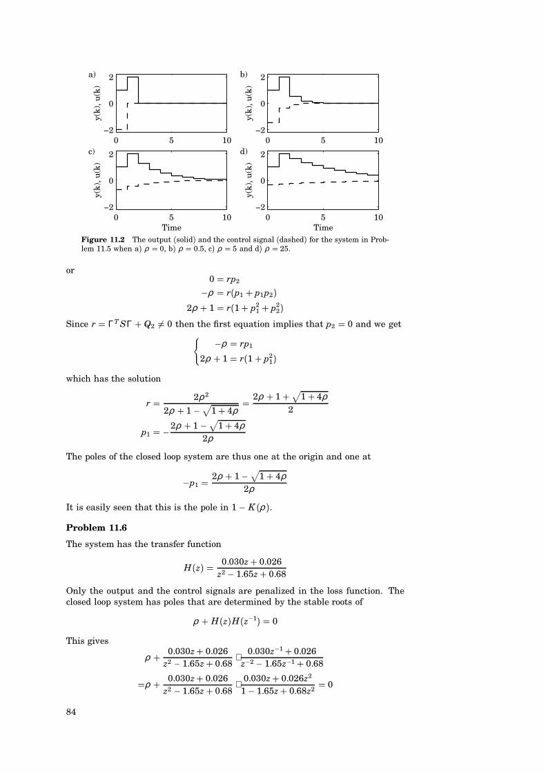
0 5 10−2
0
2
y(k)
, u(k
)
a)
0 5 10−2
0
2
y(k)
, u(k
)
b)
0 5 10−2
0
2
y(k)
, u(k
)
Time
c)
0 5 10−2
0
2
y(k)
, u(k
)
Time
d)
Figure 11.2 The output (solid) and the control signal (dashed) for the system in Prob-lem 11.5 when a) ρ 0, b) ρ 0.5, c) ρ 5 and d) ρ 25.
or0 rp2
−ρ r(p1 + p1p2)2ρ + 1 r(1+ p2
1 + p22)
Since r ΓT SΓ + Q2 6 0 then the first equation implies that p2 0 and we get−ρ rp1
2ρ + 1 r(1+ p21)
which has the solution
r 2ρ 2
2ρ + 1 −√
1+ 4ρ 2ρ + 1+√1+ 4ρ
2
p1 −2ρ + 1 −√
1+ 4ρ2ρ
The poles of the closed loop system are thus one at the origin and one at
−p1 2ρ + 1−√
1+ 4ρ2ρ
It is easily seen that this is the pole in 1 − K (ρ ).
Problem 11.6
The system has the transfer function
H(z) 0.030z+ 0.026z2 − 1.65z+ 0.68
Only the output and the control signals are penalized in the loss function. Theclosed loop system has poles that are determined by the stable roots of
ρ + H(z)H(z−1) 0
This gives
ρ + 0.030z+ 0.026z2 − 1.65z+ 0.68
⋅0.030z−1+ 0.026
z−2 − 1.65z−1+ 0.68
ρ + 0.030z+ 0.026z2 − 1.65z+ 0.68
⋅0.030z+ 0.026z2
1 − 1.65z+ 0.68z2 0
84
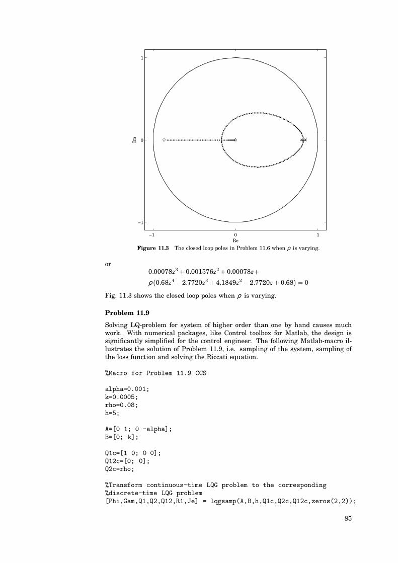
−1 0 1
−1
0
1
Re
Im
Figure 11.3 The closed loop poles in Problem 11.6 when ρ is varying.
or0.00078z3+ 0.001576z2+ 0.00078z+ρ (0.68z4 − 2.7720z3+ 4.1849z2− 2.7720z+ 0.68) 0
Fig. 11.3 shows the closed loop poles when ρ is varying.
Problem 11.9
Solving LQ-problem for system of higher order than one by hand causes muchwork. With numerical packages, like Control toolbox for Matlab, the design issignificantly simplified for the control engineer. The following Matlab-macro il-lustrates the solution of Problem 11.9, i.e. sampling of the system, sampling ofthe loss function and solving the Riccati equation.
%Macro for Problem 11.9 CCS
alpha=0.001;k=0.0005;rho=0.08;h=5;
A=[0 1; 0 -alpha];B=[0; k];
Q1c=[1 0; 0 0];Q12c=[0; 0];Q2c=rho;
%Transform continuous-time LQG problem to the corresponding%discrete-time LQG problem[Phi,Gam,Q1,Q2,Q12,R1,Je] = lqgsamp(A,B,h,Q1c,Q2c,Q12c,zeros(2,2));
85
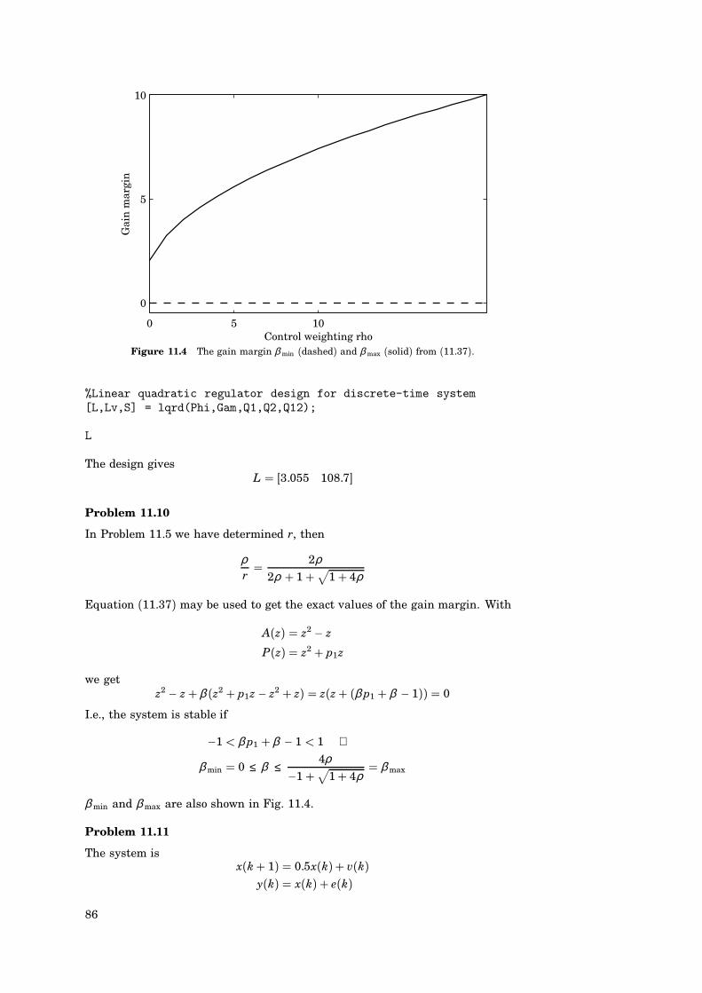
0 5 10
0
5
10
Gai
n m
argi
n
Control weighting rhoFigure 11.4 The gain margin β min (dashed) and β max (solid) from (11.37).
%Linear quadratic regulator design for discrete-time system[L,Lv,S] = lqrd(Phi,Gam,Q1,Q2,Q12);
L
The design givesL [3.055 108.7]
Problem 11.10
In Problem 11.5 we have determined r, then
ρr 2ρ
2ρ + 1+√1+ 4ρ
Equation (11.37) may be used to get the exact values of the gain margin. With
A(z) z2 − z
P(z) z2 + p1z
we getz2 − z+ β (z2 + p1z− z2 + z) z(z+ (β p1 + β − 1)) 0
I.e., the system is stable if
−1 < β p1 + β − 1 < 1 ⇒
β min 0 ≤ β ≤4ρ
−1+√1+ 4ρ β max
β min and β max are also shown in Fig. 11.4.
Problem 11.11
The system isx(k+ 1) 0.5x(k)+ v(k)
y(k) x(k) + e(k)
86
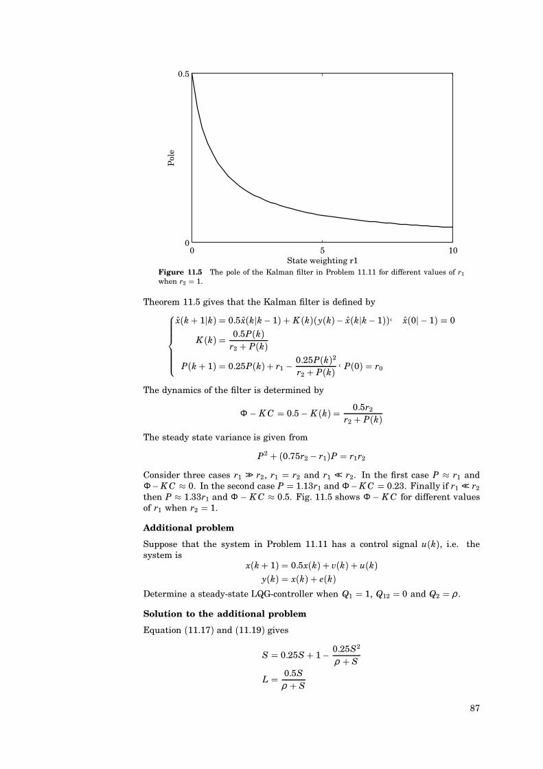
0 5 100
0.5
Pol
e
State weighting r1Figure 11.5 The pole of the Kalman filter in Problem 11.11 for different values of r1
when r2 1.
Theorem 11.5 gives that the Kalman filter is defined by
x(k+ 1jk) 0.5x(kjk− 1) + K (k)(y(k)− x(kjk− 1))A x(0j − 1) 0
K (k) 0.5P(k)r2 + P(k)
P(k+ 1) 0.25P(k)+ r1 −0.25P(k)2r2 + P(k) A P(0) r0
The dynamics of the filter is determined by
Φ − K C 0.5− K (k) 0.5r2
r2 + P(k)The steady state variance is given from
P2 + (0.75r2 − r1)P r1r2
Consider three cases r1 >> r2, r1 r2 and r1 << r2. In the first case P r1 andΦ−K C 0. In the second case P 1.13r1 and Φ−K C 0.23. Finally if r1 << r2
then P 1.33r1 and Φ − K C 0.5. Fig. 11.5 shows Φ − K C for different valuesof r1 when r2 1.
Additional problem
Suppose that the system in Problem 11.11 has a control signal u(k), i.e. thesystem is
x(k+ 1) 0.5x(k) + v(k) + u(k)y(k) x(k) + e(k)
Determine a steady-state LQG-controller when Q1 1, Q12 0 and Q2 ρ .
Solution to the additional problem
Equation (11.17) and (11.19) gives
S 0.25S + 1− 0.25S2
ρ + S
L 0.5Sρ + S
87
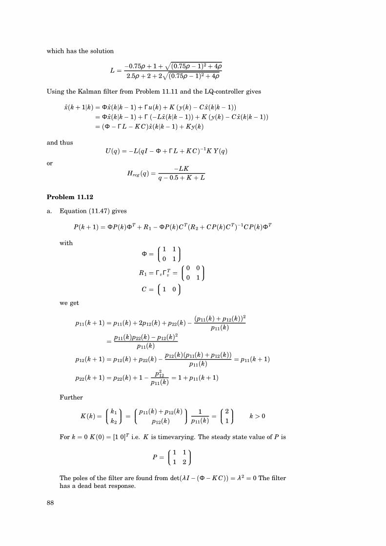
which has the solution
L −0.75ρ + 1+√(0.75ρ − 1)2 + 4ρ2.5ρ + 2+ 2
√(0.75ρ − 1)2 + 4ρ
Using the Kalman filter from Problem 11.11 and the LQ-controller gives
x(k+ 1jk) Φ x(kjk− 1) + Γu(k) + K (y(k)− Cx(kjk− 1)) Φ x(kjk− 1) + Γ (−Lx(kjk− 1)) + K (y(k)− C x(kjk− 1)) (Φ − ΓL − K C)x(kjk− 1) + K y(k)
and thusU(q) −L(qI − Φ + ΓL + K C)−1K Y(q)
or
Hreg(q) −LKq− 0.5+ K + L
Problem 11.12
a. Equation (11.47) gives
P(k+ 1) ΦP(k)ΦT + R1 − ΦP(k)CT(R2 + C P(k)CT)−1C P(k)ΦT
with
Φ 1 1
0 1
R1 ΓvΓT
v 0 0
0 1
C
1 0
we get
p11(k+ 1) p11(k) + 2p12(k) + p22(k)− (p11(k) + p12(k))2p11(k)
p11(k)p22(k)− p12(k)2p11(k)
p12(k+ 1) p12(k) + p22(k)− p12(k)(p11(k) + p12(k))p11(k) p11(k+ 1)
p22(k+ 1) p22(k) + 1 − p212
p11(k) 1+ p11(k+ 1)
Further
K (k) k1
k2
p11(k) + p12(k)p12(k)
1p11(k)
2
1
k > 0
For k 0 K (0) [1 0]T i.e. K is timevarying. The steady state value of P is
P 1 1
1 2
The poles of the filter are found from det(λ I − (Φ− K C)) λ 2 0 The filterhas a dead beat response.
88
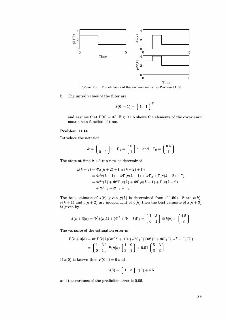
0 50
2
4
p11(
k)
Time0 5
0
2
4
p12(
k)
0 50
2
4
p22(
k)
TimeFigure 11.6 The elements of the variance matrix in Problem 11.12.
b. The initial values of the filter are
x(0j − 1) 1 1
T
and assume that P(0) 3I. Fig. 11.5 shows the elements of the covariancematrix as a function of time.
Problem 11.14
Introduce the notation
Φ 1 1
0 1
A Γ1 0
1
A and Γ2 0.5
1
The state at time k+ 3 can now be determined
x(k+ 3) Φx(k+ 2) + Γ1v(k+ 2) + Γ2
Φ2x(k+ 1) + ΦΓ1v(k+ 1) + ΦΓ2 + Γ1v(k+ 2) + Γ2
Φ3x(k) + Φ2Γ1v(k) + ΦΓ1v(k+ 1) + Γ1v(k+ 2)+ Φ2Γ2 + ΦΓ2 + Γ2
The best estimate of x(k) given y(k) is determined from (11.50). Since v(k),v(k + 1) and v(k + 2) are independent of y(k) then the best estimate of x(k + 3)is given by
x(k+ 3jk) Φ3 x(kjk)+ (Φ2 + Φ + I)Γ2 1 3
0 1
x(kjk)+ 4.5
3
The variance of the estimation error is
P(k+ 3jk) Φ3P(kjk)(Φ3)T + 0.01(Φ2Γ1ΓT1 (Φ2)T + ΦΓ1ΓT
1 ΦT + Γ1ΓT1 )
1 3
0 1
P(kjk)1 0
3 1
+ 0.015 3
3 3
If x(0) is known then P(0j0) 0 and
y(3) 1 3
x(0) + 4.5
and the variance of the prediction error is 0.05.
89

Problem 11.15
x(k+ 1) ax(k) + v(k) cov v 1
y(k) x(k) + e(k) cov e σ
We use the exponential smoothing estimator
x(kjk) α x(k− 1jk− 1) + (1 −α )y(k)
[x(kjk)−x(k)] (1−α )qq −α
y(k)−x(k)
(1 −α )qq −α
(1
q − av(k) + e(k)
)− 1
q − av(k)
− α (q − 1)(q − a)(q−α ) v(k) + (1−α )q
q −α e(k)
Using Theorem 10.4 we get
var x(kjk) 2α 2
(1+ a)(1+α )(1− aα ) +1 −αα + 1
σ
Minimize with respect to α , use Maple.
α min σ a(1+ a) + 1 −√
σ (1+ a)2 + 1σ a2(1+ a) + a− 1
Kalman with direct term
x(kjk) Φ x(k − 1jk− 1) + K (y(k)− CΦ x(k− 1jk− 1))
(I − K C)Φ x(k− 1jk− 1) + K y(k)
This will have the same form as the exponential smoothing estimator only whena 1.Kalman variance
P a2P + 1 − a2P2
P +σ((1− a2)P − 1
)(P + σ
) −a2P2
This gives
P 1 −σ (1− a2)2
+ 12
√1+ 2σ (1+ a2) + σ 2(1− a2)2
The gain in the Kalman filter is
K aPP +σ
var x(kjk) P − P2
P + σ Pσ
P + σ σ
aK
Numerical values: σ 1A a 0.5.
Exp. smoothing: α 0.4222A var x(kjk) 0.6181
Kalman: K 0.2650A var x(kjk) 0.5311
90
Problem 11.16
The scalar state equations are
x(k+ 1) ax(k) + u(k) + v(k) v(k) v1(k)+mv; Ev1 0
y(k) x(k) + e(k) e(k) e1(k)+me; Ee1 0
Let
X x mv me
T
and X(k+ 1)
a 1 0
0 1 0
0 0 1
X(k)+
1
0
0
u(k)+
1
0
0
v1(k)
y(k) 1 0 1
X(k)+ e1
The observability matrix is then
Wo
C
C A
C A2
1 0 1
a 1 1
a2 a+ 1 1
with
rank Wo 2
This means that me and mv are not both observable and no Kalman-filter can bedesigned. It is, however, possible to design a second order observer with recon-struction of a linear combination of me and mv. Redefining the state vector Xas
X x1
m
where
x1 x+me
m (a− 1)me +mv
gives X(k+ 1)
a 1
0 1
X(k)+ 1
0
u(k)+ 1
0
v1(k)
y(k) 1
0
X(k)+ e1(k)
Reconstruction of x1 and m is possible if these states are observable. The observ-ability matrix is
Wo C
CΦ
1 0
a 1
from which follows that rank Wo 2.
Problem 11.17
The constants a1 and a2 are determined by the following two conditions
1. The correct mean value should be obtained.
91
2. The variance should be minimized.Condition 1 gives that
a1 + a2 1
The variance of the estimation error is
V E(x(k)− x(k))2 E(x(k)− a1x(k)− a1e1(k)− a2x(k)− a2e2(k))2 a2
1 ⋅ 1+ a22 ⋅ 9 a2
1 + (1− a1)2 ⋅ 9 10a21 + 9 − 18a1
Taking the derivative with respect to a1 gives the condition
20a1 − 18 0 ⇐⇒ a1 910
The estimator is thusx(k) 9
10y1(k) + 1
10y2(k)
The minimum value of V isVmin 9
10Using only y1 gives the variance 1 and only y2 the variance 9. Thus, a combinationof the measurements gives a better result than using only the best measurement.Assume that the a priori estimate of x is zero and the variance of x is p, i.e.
x(0j0) and P(0j0) p
From (11.50) – (11.54) we getP(1j0) p
andK (1) P(1j0)CT (R2 + C P(1j0)CT)−1 p
10p+ 9
9 1
This gives
x(kjk) 9p10p+ 9
y1(k)+ p10p+ 9
y2(k)+ 910p+ 9
x(kjk− 1)
If p is large then the weights for y1 and y2 will be those calculated above. In theexample R1 0 the steady state gain will then be zero since the estimate willapproach the true value of x.
Problem 11.20
x(k+ 1) 1.45 −0.45
1 0
x(k) + 1
0
u(k)
y(k) 0.5 0.38
x(k)
Q1 CT C 0.25 0.19
0.19 0.1444
Q12 0
Q2 0
The steady state solution is obtained from (11.17). Using Matlab we get thesolution
⇒ S 0.25 0.19
0.19 0.1444
L
2.21 −0.45
92
An alternative solution is to use (11.40)
ρ A(z)A(z−1) + B(z)B(z−1) rP(z)P(z−1)
ρ 0 ⇒ P(z) 1b1
zB(z) 2z(0.5z+ 0.38) z(z+ 0.76)
Now we have to find L such that
(Φ − ΓL) −0.76 0
1 0
where controllable canonical form have been used. This gives
L 2.21 −0.45
Problem 11.21
a. First assume that η 0 and use linear quadratic design with
Q1 Q12 0
Q2 ρ
Q0 1
N 2
Theorem 11.1 gives the Riccati equation
S(k) 0.5(
0.5 − L(k))
S(k+ 1)
L(k) 0.5S(k)ρ + S(k+ 1)
This gives
S(N) S(2) Q0 1 ⇒ L(1) 0.5ρ + 1
S(1) 0.52ρρ + 1
⇒ L(0) 0.53
ρ + 1+ 0.52
The control law is u(k) −L(k)x(k) −Ly(k). For different values of ρ weget
ρ 1.0 0.1 0
L(0) 0.056 0.093 0.1L(1) 0.250 0.455 0.5
b. In this case η 1 and x(k) is reconstructed using a Kalman filter
x(k+ 1) 0.5x(k)+ u(k)+ K (k)(
y(k)− x(k))
withR1 R12 0
R2 η 1
R0 E(
x2(0)) 1
93
Theorem 11.5 gives
K (h) 0.5P(k)1+ P(k)
P(k+ 1) 0.25P(k)− 0.5P(k)K (k)
with P(0) R0 1. This gives
k P(k) K (k)0 1 0.251 0.125 0.056
The control law is u(k) −L(u)x(k).
Problem 11.22
x(k+ 1) x(k) + v(k)
y(k) 1
1
x(k) + e(k) R1 0.01AR2 σ 2
1 0
0 σ 22
a.
x(k+ 1jk) (
1− K 1
1
)x(kjk− 1) + K y(k)
b. (11.47) ⇒
p p+ 0.01 − p21 1
(σ 21 0
0 σ 22
+ 1
1
p 1 1
)−1 1
1
p2 1 1
σ 21 + p p
p σ 22 + p
−1 1
1
0.01
p2 σ 21 +σ 2
2
σ 21σ 2
2 + (σ 21 +σ 2
2)p 0.01
p2 − 0.01p− 0.01σ 2
1σ 22
σ 21 + σ 2
2 0
p 0.005 ±
√0.0052+ 0.01
σ 21σ 2
2
σ 21 + σ 2
2
0.005+√
0.0052 + 0.0145 0.09458
c.
K p 1 1
σ 21 + p p
p σ 22 + p
−1
σ 22 σ 2
1
σ 2
1σ 22 + p(σ 2
1 +σ 22)
p
4 1
0.094584+ 5 ⋅ 0.09458
0.0846 0.0211
94
Solutions to Chapter 12
Problem 12.1
The m-step ahead predictor is given by
y(k+mjk) qG(q)C(q) y(k)
where G is obtained from the identity (12.17) and the variance of the predictionerror is given by (12.19). For m 1 we get
q2 − 1.4q+ 0.5 q2 − 1.2q+ 0.4+ g0q+ g1
which givesG(q) g0q+ g1 −0.2q+ 0.1
The predictor is then given by
y(k+ 1jk) −0.2q2 + 0.1qq2 − 1.4q+ 0.5
y(k)
and the variance of the prediction error
E y2(k+ 1jk) σ 2 4
For m 2
q(q2 − 1.4q+ 0.5) (q2 − 1.2q+ 0.4)(q+ f1) + g0q+ g1
This givesF(q) q − 0.2G(q) −0.14q+ 0.08
andEy2(k+ 2jk) σ 2(1+ f 2
1 ) 4.16
For m 3 we get
q2(q2 − 1.4q+ 0.5) (q2 − 1.2q+ 0.4)(q2+ f1q+ f2) + g0q+ g1
which givesF(q) q2 − 0.2q− 0.14
G(q) −0.088q+ 0.056
E y2(k+ 3jk) σ 2(1+ f 21 + f 2
2 ) 4.24
Using Theorem 10.4 we can compute the variance of y to
var(y)
22 (1+1.42+0.52)(1+0.4)+2(−1.4−1.4⋅0.5)⋅1.2+2⋅0.5(1.22−0.4(1+0.4))(1− 0.42)(1+ 0.4) + (−1.2+ 1.2 ⋅ 0.4) ⋅ 1.2
4.28
This implies that the prediction variance is almost the same as the variance of ywhen m ≥ 3.
95
Problem 12.2
The identity (12.17) is
qm−1(q+ c) (q+ a)(qm−1+ f1qm−2+ ...+ fm−1) + g0
This givesc a+ f1
0 af1 + f2
...
0 afm−2 + fm−1
0 afm−1 + g0
The solution isf1 c − a
f2 (−a)(c − a)f3 (−a)2(c − a)
...
fm−1 (−a)m−2(c − a)g0 (−a)m−1(c − a)
The m-step ahead predictor is
y(k+mjk) (−a)m−1(c − a)qq+ c
y(k)
and the variance of the prediction error is
E y(k+mjk) σ 2(1+ (c − a)2 + a2(c − a)2 + ⋅ ⋅ ⋅+ a2(m−2)(c − a)2)
σ 2(
1+ (c − a)2 1 − a2(m−1)
1 − a2
)
Problem 12.3
a. The C-polynomial has a zero outside the unit circle. Example 12.1 shows howthe C-polynomial should be changed. It is replaced by
C∗(z) 5z+ 1 5(z+ 0.2)The equivalent process is thus
y(k)− 0.9y(k− 1) 5(e(k)+ 0.2e(k− 1))
b. The two-step-ahead predictor is obtained from
q(q+ 0.2) (q− 0.9)(q+ f1) + g0
This givesF(q) q+ 1.1G(g) 0.99
This predictor is
y(k+ 2jk) 0.99qq+ 0.2
y(k)
andE y2(k+ 2jk) 25(1+ 1.12) 55.25
96
Problem 12.4
Using the data given up to time k 7 it is possible to calculate y(k) and zd(k) z(k)− y(k). zd is the deterministic part of z.
k z(k) y(k) zd(k)1 320 10 3102 320 0 3203 325 −5 3304 330 −10 3405 350 0 3506 370 10 3607 375 5 370
The prediction of the demand for August through November is
z(8j7) zd(8) + y(8j7)...
z(11j7) zd(11)+ y(11j7)We thus need the 1, 2, 3 and 4 step ahead predictors of y. Those are given bysolving the identity (12.17) and give
m F(q) G(g)1 1 0.7q+ 0.12 q+ 0.7 0.59q+ 0.073 q2 + 0.7q+ 0.59 0.48q+ 0.064 q3 + 0.7q2 + 0.59q+ 0.48 0.40q+ 0.05
The prediction is
y(k+mjk) qG(q)C(q) y(k) g0 y(k) + g1 y(k− 1)
which gives the predicted values and their standard deviation σ .
m y(7+mj7) zd(7+m) z(7+mj7) σ
1 4.5 380 384.5 52 3.7 390 393.7 6.13 3.0 400 403.0 6.84 2.5 410 402.6 7.2
Problem 12.5
The polynomials areA q3 − q2 + 0.5q
B q+ 0.5
C q3 + 0.8q2+ 0.25q
It is easily seen that C is a stable polynomial, e.g. by the stability triangle. Thisis a necessary condition for the minimum variance design method.The pole excess is
d deg A − deg B 2
The Diophantine equation is
qd−1 C(q) A(q) F(q)+ G(q)q(q3+ 0.8q2 + 0.25q) (q3 − q2 + 0.5q)(q+ f1) + (g0q2 + g1q+ g2)
97
Identifying coefficients of powers of q gives
0.8 −1+ f1
0.25 0.5− f1 + g0
0 0.5 f1+ g1
0 g2
Solving these equationsf1 1.8g0 −0.25+ f1 1.55
g1 −0.9g2 0
The minimum variance regulator is obtained from (12.27)
u(k) − G(q)B(q)F(q) y(k) −1.55q2+ 0.9q
(q+ 0.5)(q+ 1.8) y(k)
The loss function isEy2 0.52(1+ 1.82) 1.06
Problem 12.6
The noise sequence has a non zero mean value. Introduce
e(k) 2+ ε(k)u(k) u+ u(k)
where ε(k) is zero mean white noise. The process is now
y(k)− 0.5y(k− 1) u+ u(k− 2) + 2+ ε(k)− 0.7(2+ ε(k − 1)) u(k− 2) + ε(k) − 0.7ε(k− 1) + u+ 0.6
Choose u −0.6 and the problem is reduced to the standard problem. The identitygives
u 0.1qq− 0.2
y(k)
andu(k) 0.1q
q− 0.2y(k)− 0.6
Problem 12.7
a. The identity givesF(q) q+ c − a
G(q) a(a− c)qand the minimum variance controller is
u(k) − a(a− c)qq+ (c − a) y(k)
b. The expression above gives the optimal controller u(k) 0 if a 0. Theprocess is then a moving average process of first order. This implies thatu(k− 2) cannot be used to decrease the variance of y(k).
98
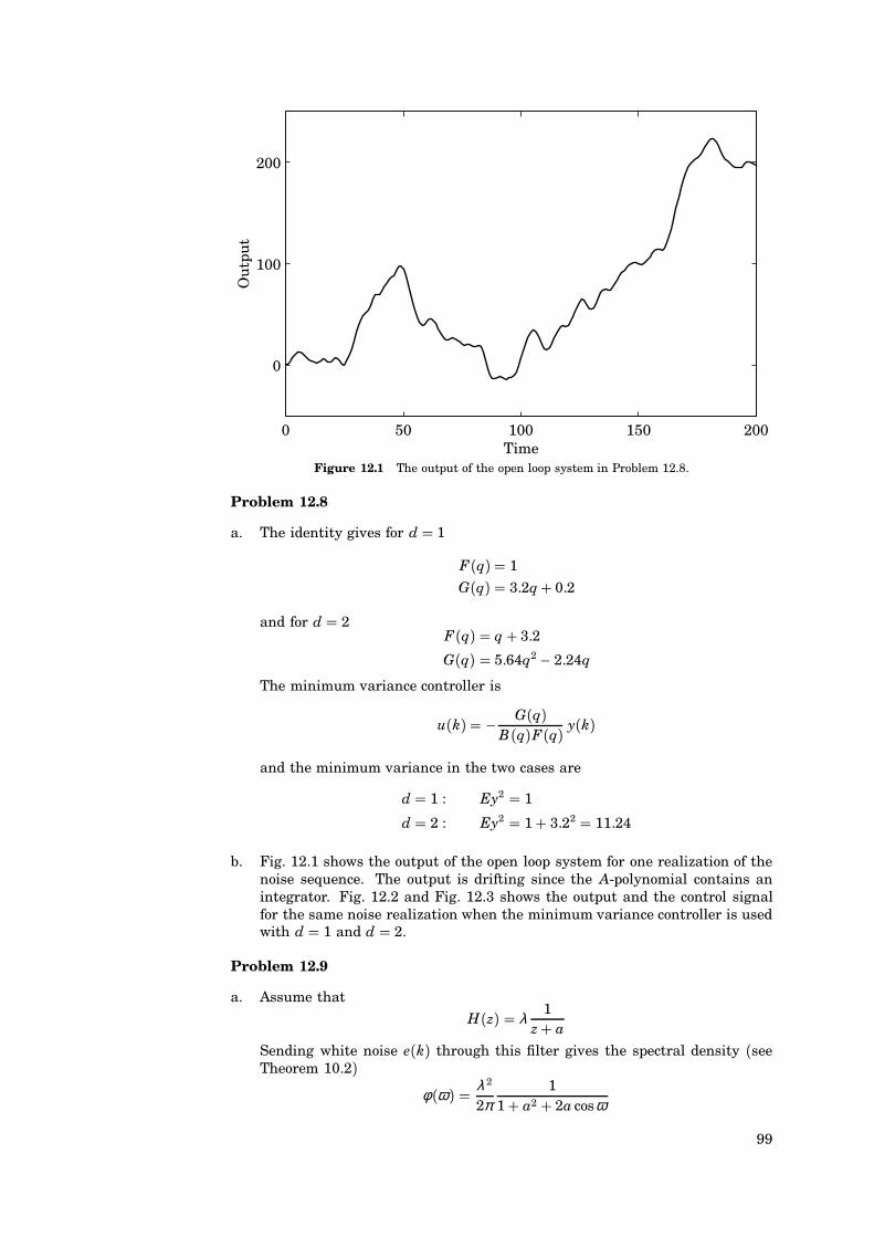
0 50 100 150 200
0
100
200
Ou
tpu
t
TimeFigure 12.1 The output of the open loop system in Problem 12.8.
Problem 12.8
a. The identity gives for d 1
F(q) 1
G(q) 3.2q+ 0.2
and for d 2F(q) q+ 3.2
G(q) 5.64q2 − 2.24q
The minimum variance controller is
u(k) − G(q)B(q)F(q) y(k)
and the minimum variance in the two cases are
d 1 : Ey2 1
d 2 : Ey2 1+ 3.22 11.24
b. Fig. 12.1 shows the output of the open loop system for one realization of thenoise sequence. The output is drifting since the A-polynomial contains anintegrator. Fig. 12.2 and Fig. 12.3 shows the output and the control signalfor the same noise realization when the minimum variance controller is usedwith d 1 and d 2.
Problem 12.9
a. Assume that
H(z) λ 1z+ a
Sending white noise e(k) through this filter gives the spectral density (seeTheorem 10.2)
φ (ω) λ 2
2π1
1+ a2 + 2a cosω
99
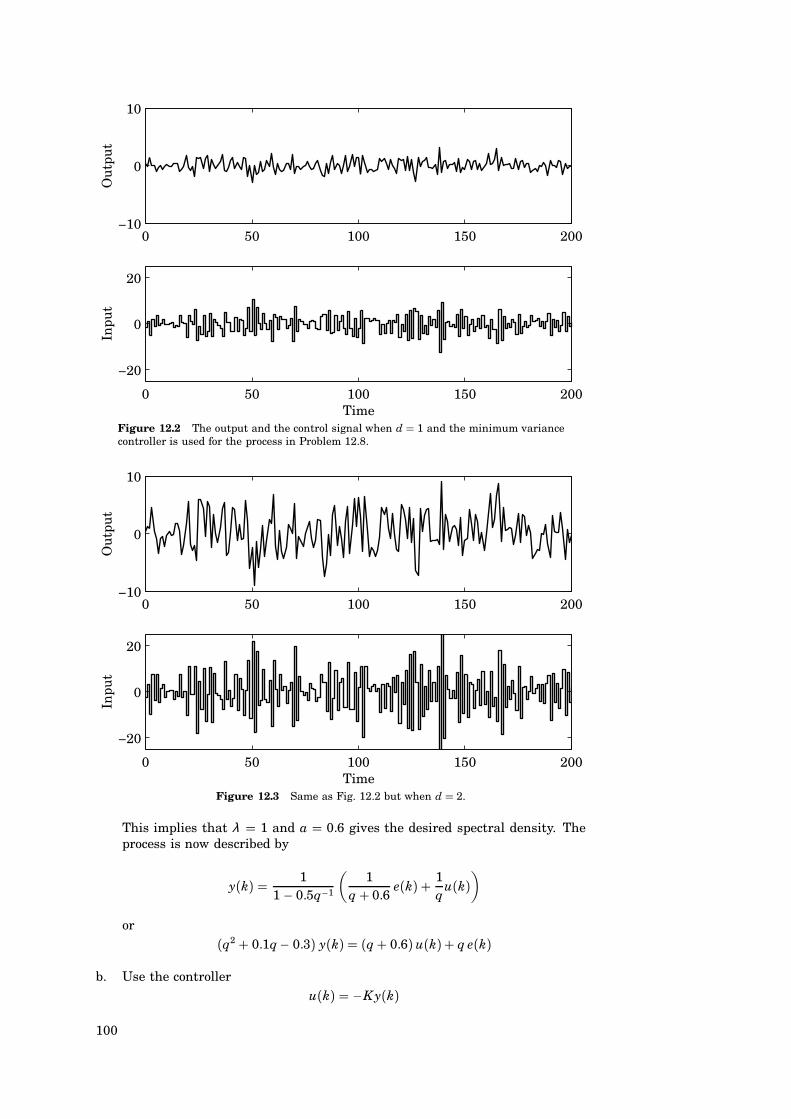
0 50 100 150 200−10
0
10O
utpu
t
0 50 100 150 200
−20
0
20
Inpu
t
TimeFigure 12.2 The output and the control signal when d 1 and the minimum variancecontroller is used for the process in Problem 12.8.
0 50 100 150 200−10
0
10
Out
put
0 50 100 150 200
−20
0
20
Inpu
t
TimeFigure 12.3 Same as Fig. 12.2 but when d 2.
This implies that λ 1 and a 0.6 gives the desired spectral density. Theprocess is now described by
y(k) 11 − 0.5q−1
(1
q+ 0.6e(k) + 1
qu(k)
)or
(q2 + 0.1q− 0.3) y(k) (q+ 0.6)u(k)+ q e(k)
b. Use the controlleru(k) −K y(k)
100
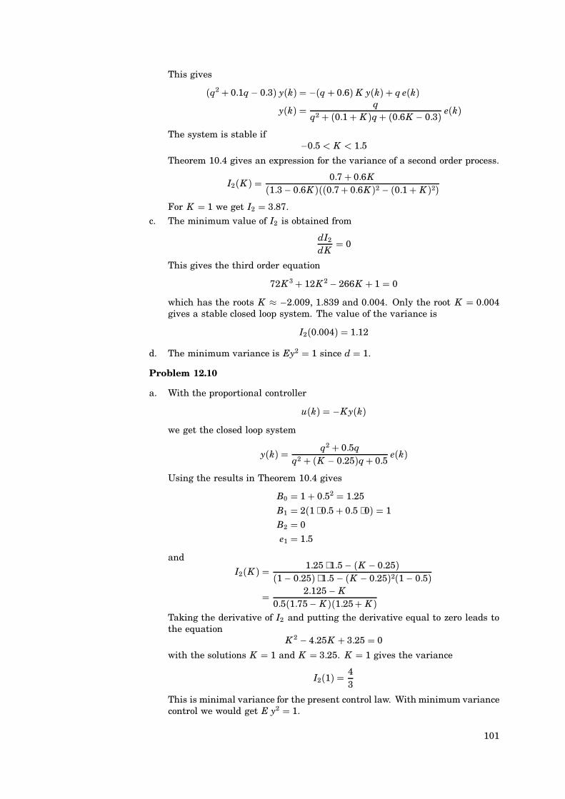
This gives
(q2 + 0.1q− 0.3) y(k) −(q+ 0.6) K y(k) + q e(k)y(k) q
q2 + (0.1+ K )q+ (0.6K − 0.3) e(k)
The system is stable if−0.5 < K < 1.5
Theorem 10.4 gives an expression for the variance of a second order process.
I2(K ) 0.7+ 0.6K(1.3− 0.6K )((0.7+ 0.6K )2 − (0.1+ K )2)
For K 1 we get I2 3.87.
c. The minimum value of I2 is obtained from
dI2
dK 0
This gives the third order equation
72K 3+ 12K 2 − 266K + 1 0
which has the roots K −2.009, 1.839 and 0.004. Only the root K 0.004gives a stable closed loop system. The value of the variance is
I2(0.004) 1.12
d. The minimum variance is Ey2 1 since d 1.
Problem 12.10
a. With the proportional controller
u(k) −K y(k)we get the closed loop system
y(k) q2 + 0.5qq2 + (K − 0.25)q+ 0.5
e(k)
Using the results in Theorem 10.4 gives
B0 1+ 0.52 1.25
B1 2(1 ⋅ 0.5+ 0.5 ⋅ 0) 1
B2 0
e1 1.5
and
I2(K ) 1.25 ⋅ 1.5− (K − 0.25)(1− 0.25) ⋅ 1.5 − (K − 0.25)2(1− 0.5)
2.125− K0.5(1.75− K )(1.25+ K )
Taking the derivative of I2 and putting the derivative equal to zero leads tothe equation
K 2 − 4.25K + 3.25 0
with the solutions K 1 and K 3.25. K 1 gives the variance
I2(1) 43
This is minimal variance for the present control law. With minimum variancecontrol we would get E y2 1.
101
b. From Example 3.2 we find that the closed loop system is stable if
0.5 > −1+ K − 0.25
0.5 > −1 − K + 0.25
or−1.25 < K < 1.75
Both K 3.25 (the second root in a.) and K 2.125 give an unstable closedloop system and the calculation of I2 is no longer valid.
Problem 12.11
y(k)− 1.5y(k− 1) + 0.7y(k− 2) u(k− 2)− 0.5u(k− 3) + v(k)gives
A(q) q3 − 1.5q2 + 0.7q
B(q) q− 0.5
Note that the process zero (0.5) is stable and well damped. This means that theprocess zero can be cancelled without problem. The degree conditions gives
deg Am − deg Bm ≥ deg A − deg B 2
deg Ao ≥ 2 deg A − deg Am − deg B+ − 1
a. v(k) 0; Deadbeat Control
Am(q) q2
B+(q) q− 0.5B−(q) 1
B ′m(q) 1
Ao(q) q2
The polynomials R1 and S are obtained from the Diophantine equation
A(z)R1(z) + B−(z)S(z) Am(z)Ao(z)Recalling the condition deg S deg A − 1 the equation becomes
(z3 − 1.5z2 + 0.7z)(z+ r1) + s0z2 + s1z+ s2 z4
with solutionr1 1.5s0 1.5r1 − 0.7 1.55
s1 −0.7r1 −1.05
s2 0
This gives the regulator
u(k) T(q)R(q) uc(k)− S(q)
R(q) y(k)
whereR(q) R1(q)B+(q) (q+ 1.5)(q− 0.5)T(q) Bm Ao q2
Assuming that uc(k) 0 gives
u(k) −S(q)R(q) y(k) − 1.55q2 − 1.05q
(q+ 1.5)(q− 0.5)
102
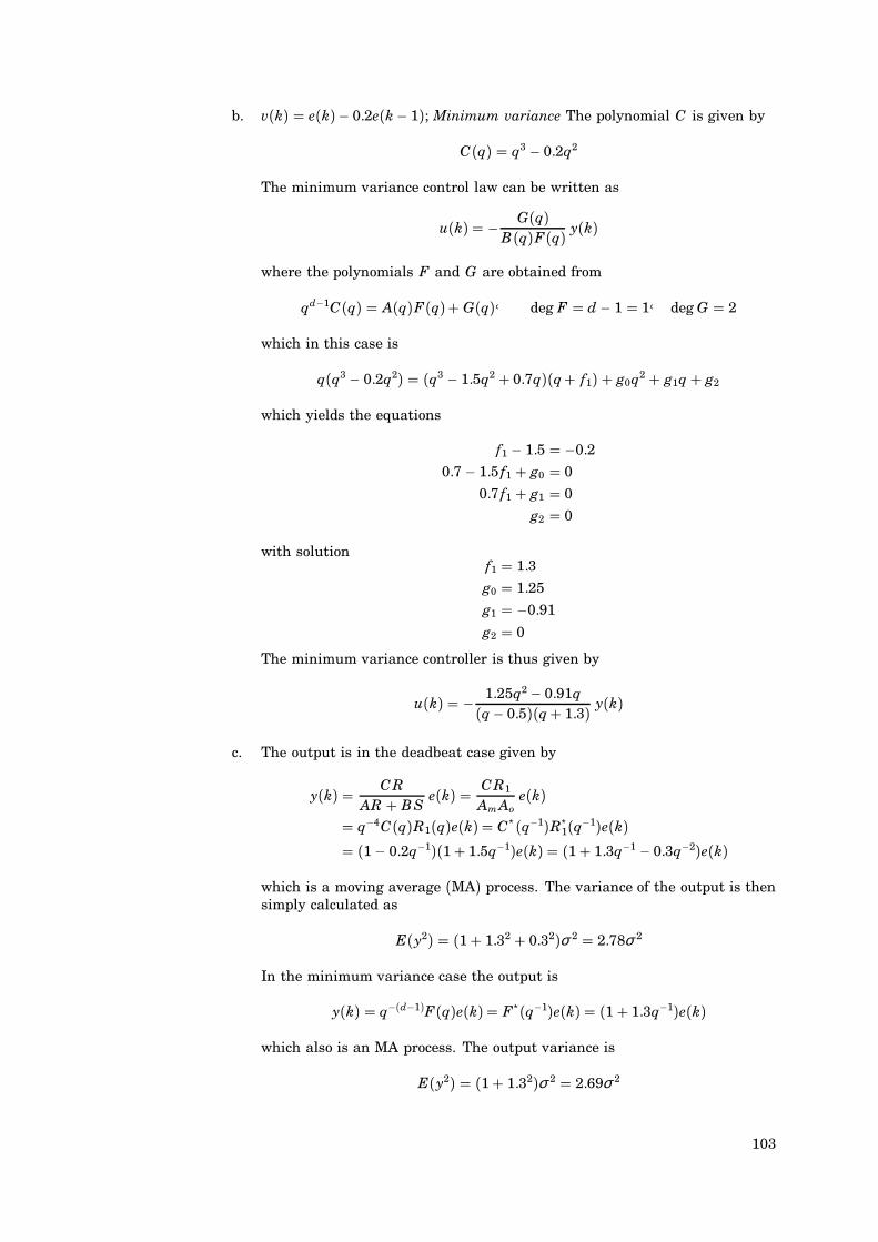
b. v(k) e(k)− 0.2e(k− 1); Minimum variance The polynomial C is given by
C(q) q3 − 0.2q2
The minimum variance control law can be written as
u(k) − G(q)B(q)F(q) y(k)
where the polynomials F and G are obtained from
qd−1C(q) A(q)F(q)+ G(q)A deg F d− 1 1A deg G 2
which in this case is
q(q3 − 0.2q2) (q3 − 1.5q2 + 0.7q)(q+ f1) + g0q2 + g1q+ g2
which yields the equations
f1 − 1.5 −0.20.7 − 1.5 f1 + g0 0
0.7 f1 + g1 0
g2 0
with solutionf1 1.3g0 1.25
g1 −0.91
g2 0
The minimum variance controller is thus given by
u(k) − 1.25q2 − 0.91q(q− 0.5)(q+ 1.3) y(k)
c. The output is in the deadbeat case given by
y(k) C RAR + B S
e(k) C R1
Am Aoe(k)
q−4C(q)R1(q)e(k) C∗(q−1)R∗1(q−1)e(k)
(1− 0.2q−1)(1+ 1.5q−1)e(k) (1+ 1.3q−1 − 0.3q−2)e(k)
which is a moving average (MA) process. The variance of the output is thensimply calculated as
E(y2) (1+ 1.32 + 0.32)σ 2 2.78σ 2
In the minimum variance case the output is
y(k) q−(d−1)F(q)e(k) F∗(q−1)e(k) (1+ 1.3q−1)e(k)
which also is an MA process. The output variance is
E(y2) (1+ 1.32)σ 2 2.69σ 2
103
0 50 100 150 200−10
0
10O
utpu
t
0 50 100 150 200−10
0
10
Out
put
0 50 100 150 2000
500
Los
s
TimeFigure 12.4 The output and the sum of the square of the output for the two regulatorsin Problem 12.11. The deadbeat controller is used in the upper diagram and the minimumvariance controller in the middle diagram. The accumulated loss functions are shown inthe lower diagram, deeadbeat (dashed) and minimum variance (solid).
d. Fig. 12.5 shows the output and the sum of the square of the output for theregulators in a and b.
Problem 12.12
Introduce the polynomialsA1(q) A(q)D(q)B1(q) B(q)D(q)C1(q) A(q)C(q)
and the noise e1 λ e. The system can then be written as
y(k) B1
A1u(k) + λ C1
A1e1(k) (12.1)
Since A, C and D are monic, A1 AD and C1 AC will also bo monic. Letd1 deg A1 − deg B1 deg A − deg B d. The minimum-variance controller forthe rewritten system (12.1) is then calculated as
u(k) − G1(q)B1(q)F1(q) y(k) (12.2)
whereqd1−1C1(q) A1(q)F1(q) + G1(q) (12.3)
Equation (12.3) is equivalent to
qd−1A(q)C(q) A(q)D(q)F1(q) + G1(q)
which implies that A must divide G1, i.e. G1(q) A(q)G(q). Putting F F1
gives the minimum-variance control law
u(k) − G(q)A(q)B(q)D(q)F(q) y(k) − G∗(q−1)A∗(q−1)
B∗(q−1)D∗(q−1)F∗(q−1) y(k)
104
where F and G satisfy the equation
qd−1C(q) D(q)F(q)+ G(q)
with deg F d − 1 and deg G deg D − 1. We see that if A D the controllerreduces to the normal minimum variance controller.
Problem 12.13
In this caseA(q) q+ a
B(q) b
C(q) q+ c
D(q) q
d 1
The identity in Problem 12.12 gives
q+ c q ⋅ 1+ g0
⇒ g0 c
The minimum variance controller is thus
u(k) − c(q+ a)bq
y(k) − cb
y(k)− acb
y(k− 1)
Problem 12.15
We have
y1(k) 11− 0.7q−1 u(k− 1) + 1− 0.5q−1
1− 0.7q−1 e(k)
y2(k) q−1
1+α q−1 y1(k)
1A∗
1
(B∗
A∗u(k− 2) + C∗
A∗e(k− 1)
) 1(1+α q−1)(1− 0.7q−1) u(k− 2) + 1 − 0.5q−1
(1+α q−1)(1− 0.7q−1) e(k− 1)
To normalize the notations it is convenient to introduce a new noise ε (k) e(k−1).a. Assume that y1 can be measured. The minimum variance controller for y1 is
then
u(k) −0.2y1(k)
b. The variances of y1 and y2 are
Ey21 1
Ey22
11 − α 2 2.78
105
c. The minimum variance controller for y2 when y2 is measurable is obtainedby using the identity
1 − 0.5q−1 (1+α q−1)(1− 0.7q−1)(1+ f1q−1) + q−2(g0 + g1q−1)
This givesF∗(q−1) 1+ q−1
G∗(q−1) 0.94− 0.56q−1
and the controller
u(k) −0.94 − 0.56q−1
1+ q−1 y2(k)
This givesy2(k) (1+ q−1)ε (k) ε (k− 1) + e(k− 2)
andy1(k) (1+ q−1)(1+α q−1)e(k+ 1)
The variances of the two signals are
Ey21 1+ (α + 1)2 +α 2 1.68
Ey22 1+ 1 2
d. In this case both y1 and y2 are measurable and y1(k)will contain more recentinformation about the noise process than y2(k). It is now only necessary topredict one step ahead. Introduce the identity
C∗ A∗ A∗1 + q−1G∗
1
This gives
y2(k+ 2) C∗
A∗1 A∗
e(k+ 2) + B∗
A∗1 A∗
u(k)
e(k+ 2) + G∗1
A∗1 A∗
e(k+ 1) + B∗
A∗1 A∗
u(k)
But
ε (k+ 1) A∗
C∗y1(k)− B∗
C∗u(k− 1)
This gives
y2(k+ 2) ε (k+ 2) + G∗1
A∗1 A∗
(A∗
C∗y1(k)− B∗
C∗u(k− 1)
)+ B∗
A∗1 A∗
u(k)
ε (k+ 2) + G∗1
A∗1 A∗
y1(k) + B∗
A∗1 A∗ C∗
(C∗ − G∗
1q−1) u(k)
ε (k+ 2) + 1C∗
(G∗
1
A∗1
y1(k) + B∗u(k))
The variance is thus minimized when
u(k) − G∗1
A∗1 B∗
y1(k)
which is an admissible control law. For the specific system we get
u(k) −1 − 0.56q−1
1− 0.8q−1 y1(k)
106
With this control law we get
y2(k) ε (k) e(k− 1)
and
y1(k) (1+α q−1)y2(k+ 1) (1+α q−1)ε (k+ 1) (1+α q−1)e(k)
The variances of the two output signals are
Ey21 1+α 2 1.64
andEy2
2 1
We can thus conclude that the extra measurement will greatly improve thecontrol of the output of the system.
Problem 12.16
The same arguments can be used in this case as when deriving the normal min-imum variance controller. Assume that the system has a stable inverse. Alsoassume that deg A deg B deg D i.e. that the process can be written as
A∗(q−1)y(k) B∗(q−1)u(k− d) + C∗(q−1)e(k)+ D∗(q−1)v(k− d)
The identity (12.17) can be used here also and gives
y(k+ d) C∗
A∗e(k+ d) + B∗
A∗u(k) + D∗
A∗v(k)
F∗e(k+ d) + G∗
A∗e(k)+ B∗
A∗u(k) + D∗
A∗v(k)
F∗e(k+ d) + G∗
A∗
(A∗
C∗y(k)− B∗
C∗u(k− d)− D∗
C∗v(k − d)
)+ B∗
A∗u(k)+ D∗
A∗v(k)
F∗e(k+ d) + G∗
C∗y(k) + B∗
A∗C∗
(C∗ − q−dG∗
)u(k)
+ D∗
A∗C∗
(C∗ − q−dG∗
)v(k)
F∗e(k+ d) + 1C∗(G∗ y(k)+ B∗ F∗u(k)+ D∗F∗v(k))
The minimum variance controller is thus
u(k) − G∗
B∗ F∗y(k)− D∗
B∗v(k)
Problem 12.17
A(q)y(k) B(q)u(k)+ C(q)e(k)A(q) q − 0.9A B(q) qA C(q) q − 0.5
LQG-Control: Minimize E(y2 + ρ u2). Let P(z) be the closed loop system char-acteristic equation (12.45)
rP(z)P(z−1) ρ A(z)A(z−1) + B(z)B(z−1)
107
P(z) contains stable zeros of the right hand expression (Lemma 12.1)
r(z+ p1)(z−1+ p1) ρ (z− 0.9)(z−1 − 0.9) + 1 ⋅ 1
r(1+ p21) + rp1z+ rp1z−1 1.81ρ + 1 − 0.9ρ z−1 − 0.9ρ z
This gives the system of equations
rp1 −0.9ρr(1+ p2
1) 1+ 1.81ρ
which has two solutions, one of which gives a stable P(z)
p1 −1+ 1.81ρ1.8ρ +
√(1+ 1.81ρ
1.8ρ )2 − 1
Determine the LQG-regulator by means of pole placement:
Am P(z) z+ p1
Ao C(z) z− 0.5
Control law:
u(k) −S(q)R(q) y(k)
where S(0) 0. See computational procedure in Section 12.5.The Diophantine equation to be solved is
PC AR + B S
or(z+ p1)(z− 0.5) (z− 0.9)(z+ r1) + zs0
This givesp1 − 0.5 −0.9+ r1 + s0
−0.5p1 −0.9r1
The solution is given by
r1 59
p1
s0 0.4+ 49
p1
which results in the controller
u(k) − s0qq+ r1
y(k)
For the closed loop system we get
y(k) BA
u(k) + CA
e(k) BA
(−S
Ry(k)
)+ C
Ae(k)
or
y(k) C RAR + B S
e(k) C RPC
e(k) RP
e(k) q+ r1
q+ p1e(k)
Theorem 10.4 gives
Var y 1+ r21 − 2r1p1
1 − p21
108
The input u is
u(k) −SR
y(k) −SR
⋅RP
e(k) −SP
e(k) − s0qq+ p1
e(k)
Theorem 10.4 gives
Var u s20
1− p21
In the following table the calculations are summarized for ρ 0.1A1 and 10.
ρ p1 Var y Var u
0.1 −0.077 1.0012 0.1351 −0.36 1.030 0.0658
10 −0.70 1.197 0.0148
Problem 12.24
From Example 12.16 we get a polynomial description of the process
A(q)y(k) B(q)u(k)+ C(q)e(k)
whereA(q) q− 1
B(q) h
C(q) q+ c
The minimum variance regulator is given by the Diophantine
PC AR + B S
whereP(q) qd−1B(q) h
The solution isr0 h
s0 c + 1
and the minimum variance regulator is
u(k) − c + 1h
y(k)
In LQ − design we use a state-space description of the process (see Example12.16)
x(kh+ h) x(kh) + hu(kh)+ v(kh+ h) − v(kh)y(kh) x(kh) + ε(kh)
To obtain the LQ-controller we have to sample the loss function.From (11.6) - (11.8) we get
Q1 ∫ h
01 ⋅ ds h
Q12 ∫ h
0s ⋅ ds h2
2
Q2 ∫ h
0s2 ⋅ ds h3
3
109
The Riccati equation isS ΦT SΦ + Q1 − LT (Q2 + ΓT SΓ)LL (Q2 + ΓT SΓ)−1(ΓT SΦ + Q12)
and the solution is S h√
12
L 1h
3+√32+√3
The closed loop system has a pole in −p1
−p1 Φ − ΓL 1− h1h
3+√3
2+√3√
3 − 2
andP(z) z+ p1
To get the regulator we solve the Diophantine (see p. 481)
PC AR + B S S(0) 0
(q+ p1)(q+ c) (q− 1)(q+ r1) + hs0q
which has the solutionr0 −p1c
s0 1h(p1 + c + 1+ p1c)
and thus
u(k) −1h(p1 + c + 1+ p1c)q
q− p1cy(k)
Problem 12.29
The process is described by
A(z) z2 − 1.4z+ 0.65
B(z) z− 0.2
C(z) z2 + 0.4z
a. To get the minimum variance controller we use the identity
A(z) F(z)+ G(z) zd−1 C(z)z2 − 1.4z+ 0.65+ g0z+ g1 z2 + 0.4z
This givesG(z) 1.8z− 0.65
The control law is
u − GB F
y −1.8q− 0.65q− 0.2
y
b. The dead-beat controller is obtained from the identity
A(z)F(z)+ G(z) z2
which givesG(z) 1.4z− 0.65
u −1.4q− 0.65q− 0.2
y
110

c. Minimum variance control
var(y) 1 ⋅ σ 2 4
Dead-beat controlvar(y) (1+ 0.42)σ 2 4.64
Problem 12.30
a. Assume that C 0 and use the identity
C AF + G
This givesF 1
G −a
and the controller
u − GB F
y ay
The closed loop system becomes
y(k) e(k)+ ce(k− 1)
and the variancevar(y) 1+ c2
b. Assume that C(z) z+ c. The minimum variance controller for this modelis given by
F 1
G c − a
The closed loop system is now
y(k) q+ cq+ c
e(k)
which has the variance, see Theorem 6.4
var(y) (1+ c2) − 2cc1 − c2
It is better to use a guessed value c if
0 < c < 2c1+ c2
Problem 12.31
The C polynomial has a pole outside the unit circle. Replace C by a new polyno-mial obtained from spectral factorization
C(z)C(z−1) (z− 1.25)(z−1− 1.25) 1.252(z− 0.8)(z−1 − 0.8)
The new process is
y(k) q2 − 0.8qq2 − 1.1q+ 0.3
ε (k)
where ε has the standard deviation 1.25.
111
a. The 2-step ahead predictor is given by
zm−1C(z) A(z)F(z)+ G(z)z(z2 − 0.8z) (z2 − 1.1z+ 0.3)(z+ f1) + g0z+ g1
which givesF(z) z+ 0.3
G(z) 0.03z− 0.09
and
y(k+ 2jk) qG(q)C(q) y(k) 0.03(q− 3)
q − 0.8y(k)
b. The prediction error variance is
E y 1.252(1+ 0.32) 1.70
Problem 12.32
a. d 2. This gives the identity
zC(z) A(z)F(z)+ G(z)
where deg F 1 and deg G 2, i.e.,
z3(z− 0.1) (z3 − 1.7z2+ 0.8z− 0.1)(z+ f1) + g0z2 + g1z+ g2
The solution isF(z) z+ 1.6
G(z) 1.92z2 − 1.18z+ 0.16
and the controller is
u(k) − GB F
y(k) −1.92q2 − 1.18q+ 0.162(q− 0.9)(q+ 1.6) y(k)
b. The output variance when using the minimum variance controller in a. isgiven by
var(y) 1+ f 21 1+ 1.62 3.56
c. Since B(z) has a root outside the unit circle we use the procedure in Theorem12.3. Factor B(z) as
B(z) B+(z) B−(z)with B−∗(q) monic, so
B+(z) −2
B−(z) −0.9q+ 1
The Diophantine to solve is
qd−1C(q)B−∗(q) A(q)F(q)+ B−(z)G(q)q3(q− 0.1)(q− 0.9) (q3 − 1.7q2+ 0.8q− 0.1)( f0q2 + f1q+ f2)
+ (−0.9q+ 1)(g0q2 + g1q+ g2)
112
This gives the system of equations
1 f0
−1 −1.7 f0 + f1
0.09 0.8 f0 − 1.7 f1 + f2 + 1.8g0
0 −0.1 f0 + 0.8 f1 − 1.7 f2 − 2g0 + 1.8g1
0 −0.1 f1 + 0.8 f2 − 2g1 + 1.8g2
0 −0.1 f2 − 2g2
which has the solutionf0 1.000
f1 0.700
f2 2.721
g0 2.490
g1 −1.862
g2 0.272
Equation (12.31) gives
u(k) − G(q)B+(q)F(q) y(k) −−1.245q2+ 0.931q− 0.136
q2 + 0.7q+ 2.721y(k)
The closed loop system is
Ay(k) Bu(k) + Ce(k) B(− G
B+Fy(k)
)+ Ce(k)
−GB−
Fy(k) + Ce(k)
or
y(k) C FAF + GB−
e(k) C Fqd−1C B−∗
e(k) Fqd−1B−∗
e(k)
q2 + 0.7q+ 2.721q(q− 0.9) e(k)
Theorem 10.4 gives the output variance
Var y 94.7
Problem 12.33
y(k) 0.9q+ 1(q− 1)(q− 0.7) u(k) + q(q− 0.7)
(q− 1)(q− 0.7) e(k)
Determine the controller from
AR + B S qd−1C
(q− 1)(q− 0.7)(q+ r1) + (0.9q+ 1)(s0q+ s1) q2(q− 0.7)This gives the system of equations
−1.7+ r1 + 0.9s0 −0.7
0.7− 1.7r1 + 0.9s1 + s0 0
0.7r1 + s1 0
113

with the solutionr1 0.526
s0 0.526
s1 −0.368
y(k) C RAR + B S
e(k) C RqC
(1+ 0.526q−1)e(k)
var y(k) (1+ 0.5262)σ 2 1.27σ 2
Compare to Example 12.9 p. 468
var y(k) 2019
σ 2 1.053σ 2
114


![Automotive Computer Controlled Systems [h33t] [Malestrom]](https://img.pdfslide.us/doc/110x75/5456ec91b1af9fda448b4b33/automotive-computer-controlled-systems-h33t-malestrom-55844f1bd285e.jpg)