airwalkbooks.comairwalkbooks.com/images/pdf/pdf_123_1.pdf · Computer Aided Design and Manufacturing (For B.E. / B.Tech Mechanical Engineering Students) As per the Latest Syllabus

Computer Aided Designand

Manufacturing (For B.E. / B.Tech Mechanical Engineering Students)

As per the Latest Syllabus of Anna University

Email : [email protected], [email protected]

www.airwalkbooks.com, www.srbooks.org

80, KARNEESHWARA KOIL STREET,

(Near All India Radio) MYLAPORE, CHENNAI - 4

Ph.: 044 - 24661909, 9444081904

AIRWALK PUBLICATIONS

Dr. S. Ramachandran

P. Vijayalakshmi

D.Jagadhish

Professor - Mech Sathyabama Institute of Science & Technology

Chennai - 600 119.

250/-

and

First Edition : 16-11-19

www.airwalkbooks.com www.srbooks.org and

Cell: 9600003081, 9600003082

Typeset by: aksharaa muthra aalayam pvt. ltd., Chennai - 18. Ph.: 044-2436 4303

ISBN: 978-93-88084-50-5

ISBN: 978-93-88084-50-5

ME8691 COMPUTER AIDED DESIGN AND MANUFACTURING

UNIT I: INTRODUCTION 9

Product cycle – Design process – sequential and concurrent engineering– Computer aided design – CAD system architecture – Computer graphics –co-ordinate systems-2D and 3D transformations – homogeneous coordinates –Line drawing – Clipping-viewing transformation – Brief introduction to CADand CAM – Manufacturing Planning, Manufacturing control – Introduction toCAD/CAM – CAD/CAM concepts – Types of production – Manufacturingmodels and Metrics – Mathematical models of Production Performance

UNIT II: GEOMETRIC MODELING 9

Representation of curves-Hermite curve-Bezier curve-B-splinecurves-rational curves-Techniques for surface modeling – surface patch –Coons and bicubic patches – Bezier and B-spline surfaces. Solid modelingtechniques – CSG and B-rep

UNIT III: CAD STANDARDS 9

Standards for computer graphics-Graphical Kernel System (GKS) –standards for exchange images – Open Graphics Library (OpenGL) – Dataexchange standards -IGES, STEP, CALS etc. – communication standards.

UNIT IV: FUNDAMENTAL OF CNC AND PART PROGRAMING 9

Introduction to NC systems and CNC – Machine axis and Co-ordinatesystem – CNC machine tools – Principle of operation CNC – Constructionfeatures including structure – Drives and CNC controllers 2D and 3D machiningon CNC – Introduction of Part Programming, types – Detailed Manual partprogramming on Lathe & Milling machines using G codes and M codes – CuttingCycles, Loops, Sub program and Macros-Introduction of CAM package.

UNIT V: CELLULAR MANUFACTURING AND FLEXIBLE MANUFACTURING SYSTEM (FMS) 9

Group Technology (GT), Part Families – Parts Classification andcoding – Simple Problems in Opitz Part Coding system – Production flowAnalysis – Cellular Manufacturing – Composite part concept – Types ofFlexibility – FMS – FMS Components – FMS Application & Benefits – FMSPlanning and Control – Quantitative analysis in FMS

TOTAL : 45 PERIODS

Table of Contents

UNIT I: INTRODUCTION

1.1 Introduction . . . . . . . . . . . . . . . . . . . . . . . . . . . . . . . . . . . . . . . . . . . . . . 1.1

1.2 Product Cycle . . . . . . . . . . . . . . . . . . . . . . . . . . . . . . . . . . . . . . . . . . . . 1.2

1.3 Design Process . . . . . . . . . . . . . . . . . . . . . . . . . . . . . . . . . . . . . . . . . . . 1.4

1.4 Sequential Engineering . . . . . . . . . . . . . . . . . . . . . . . . . . . . . . . . . . . . 1.8

1.5 Concurrent Engineering . . . . . . . . . . . . . . . . . . . . . . . . . . . . . . . . . . . . 1.9

1.6 Comparison of Sequential and Concurrent Engineering . . . . . . . . 1.11

1.7 Computer Aided Design . . . . . . . . . . . . . . . . . . . . . . . . . . . . . . . . . . 1.13

1.7.1 Why should we go for CAD? . . . . . . . . . . . . . . . . . . . . . . . 1.13

1.7.2 Factors considered for selecting CAD system . . . . . . . . . . 1.14

1.7.3 Role of computer in CAD . . . . . . . . . . . . . . . . . . . . . . . . . . 1.14

1.8 Benefits of CAD . . . . . . . . . . . . . . . . . . . . . . . . . . . . . . . . . . . . . . . . 1.15

1.9 Engineering Applications of CAD . . . . . . . . . . . . . . . . . . . . . . . . . . 1.16

1.10 Computer Graphics . . . . . . . . . . . . . . . . . . . . . . . . . . . . . . . . . . . . . 1.19

1.11 Coordinate Representation System . . . . . . . . . . . . . . . . . . . . . . . . . 1.20

1.11.1 Cartesian coordinate system . . . . . . . . . . . . . . . . . . . . . . . 1.20

1.11.2 World coordinate system . . . . . . . . . . . . . . . . . . . . . . . . . . 1.21

1.11.3 Normalised coordinate system . . . . . . . . . . . . . . . . . . . . . . 1.21

1.11.4 Device coordinate system . . . . . . . . . . . . . . . . . . . . . . . . . . 1.22

1.12 Two Dimensional Transformation . . . . . . . . . . . . . . . . . . . . . . . . . 1.23

1.12.1 Translation . . . . . . . . . . . . . . . . . . . . . . . . . . . . . . . . . . . . . . 1.23

1.12.2 Scaling . . . . . . . . . . . . . . . . . . . . . . . . . . . . . . . . . . . . . . . . . 1.29

1.12.3 Rotation . . . . . . . . . . . . . . . . . . . . . . . . . . . . . . . . . . . . . . . . 1.31

1.13 Three Dimensional Transformations . . . . . . . . . . . . . . . . . . . . . . . . 1.39

1.13.1 Translation . . . . . . . . . . . . . . . . . . . . . . . . . . . . . . . . . . . . . . 1.39

1.13.2 Scaling . . . . . . . . . . . . . . . . . . . . . . . . . . . . . . . . . . . . . . . . . 1.40

Contents C.1

1.13.3 Rotation . . . . . . . . . . . . . . . . . . . . . . . . . . . . . . . . . . . . . . . . 1.40

1.14 Homogeneous Coordinates Representation . . . . . . . . . . . . . . . . . . 1.41

1.15 Homogeneous Transformation Matrices . . . . . . . . . . . . . . . . . . . . . 1.43

1.15.1 Translation . . . . . . . . . . . . . . . . . . . . . . . . . . . . . . . . . . . . . . 1.43

1.15.2 Scaling . . . . . . . . . . . . . . . . . . . . . . . . . . . . . . . . . . . . . . . . . 1.43

1.15.3 Rotation . . . . . . . . . . . . . . . . . . . . . . . . . . . . . . . . . . . . . . . . 1.43

1.15.4 Shear . . . . . . . . . . . . . . . . . . . . . . . . . . . . . . . . . . . . . . . . . . . 1.44

1.15.5 Application of homogeneous coordinate representation . 1.44

1.16 Line Drawing . . . . . . . . . . . . . . . . . . . . . . . . . . . . . . . . . . . . . . . . . . 1.45

1.17 Clipping . . . . . . . . . . . . . . . . . . . . . . . . . . . . . . . . . . . . . . . . . . . . . . . 1.57

1.17.1 Cohen - Sutherland line clipping algorithm . . . . . . . . . . 1.58

1.18 Viewing Transformation . . . . . . . . . . . . . . . . . . . . . . . . . . . . . . . . . 1.60

1.19 Brief Introduction to CAD and CAM . . . . . . . . . . . . . . . . . . . . . . 1.62

1.20 Computer Aided Design (CAD) . . . . . . . . . . . . . . . . . . . . . . . . . . . 1.62

1.21 Design Process In CAD System (or) Elements of a CAD . . . . 1.67

1.21.1 Geometric modeling . . . . . . . . . . . . . . . . . . . . . . . . . . . . . . 1.68

1.21.2 Engineering Analysis . . . . . . . . . . . . . . . . . . . . . . . . . . . . . . 1.69

1.22 Computer Aided Manufacturing (CAM) . . . . . . . . . . . . . . . . . . . . 1.70

1.23 Concurrent Engineering . . . . . . . . . . . . . . . . . . . . . . . . . . . . . . . . . . 1.75

1.24 Introduction of CIM . . . . . . . . . . . . . . . . . . . . . . . . . . . . . . . . . . . . 1.80

1.25 CASA/SME Model of CIM/CIM Wheel . . . . . . . . . . . . . . . . . . . . 1.82

1.26 Nature and Role of the Elements of CIM System . . . . . . . . . . . 1.83

1.27 Reasons for Implementing CIM . . . . . . . . . . . . . . . . . . . . . . . . . . . 1.86

1.28 Objectives/Goal of CIM . . . . . . . . . . . . . . . . . . . . . . . . . . . . . . . . . 1.87

1.29 CIM I vs CIM II . . . . . . . . . . . . . . . . . . . . . . . . . . . . . . . . . . . . . . . 1.88

1.30 Benefits of CIM . . . . . . . . . . . . . . . . . . . . . . . . . . . . . . . . . . . . . . . . 1.88

C.2 Computer Aided Design and Manufacturing - www.airwalkbooks.com

1.31 Computer Integrated Manufacturing (CIM) as a Concept and a

Technology . . . . . . . . . . . . . . . . . . . . . . . . . . . . . . . . . . . . . . . . . . . . 1.89

1.32 Computerised Elements of a CIM-System . . . . . . . . . . . . . . . . . . 1.90

1.33 Types of Production . . . . . . . . . . . . . . . . . . . . . . . . . . . . . . . . . . . . 1.91

(i) Job shop Production . . . . . . . . . . . . . . . . . . . . . . . . . . . . . . . . . 1.92

(ii) Batch production . . . . . . . . . . . . . . . . . . . . . . . . . . . . . . . . . . . 1.93

(iii) Mass Production . . . . . . . . . . . . . . . . . . . . . . . . . . . . . . . . . . . 1.93

1.34 Manufacturing Models and Metrics . . . . . . . . . . . . . . . . . . . . . . . . 1.94

1.35 Mathematical Models of Production Performance . . . . . . . . . . . . 1.95

1.36 Manufacturing Costs . . . . . . . . . . . . . . . . . . . . . . . . . . . . . . . . . . . 1.102

1.36.1 Fixed and variable costs . . . . . . . . . . . . . . . . . . . . . . . . . 1.102

1.36.2 Direct labour, Material, and overhead . . . . . . . . . . . . . . 1.103

1.37 Manufacturing Control . . . . . . . . . . . . . . . . . . . . . . . . . . . . . . . . . . 1.108

UNIT II: GEOMETRIC MODELING

2.1 Introduction . . . . . . . . . . . . . . . . . . . . . . . . . . . . . . . . . . . . . . . . . . . . . . 2.1

2.2 Representation of Curves . . . . . . . . . . . . . . . . . . . . . . . . . . . . . . . . . . 2.1

2.2.1 Analytic curve . . . . . . . . . . . . . . . . . . . . . . . . . . . . . . . . . . . . . 2.2

2.2.2 Synthetic curves . . . . . . . . . . . . . . . . . . . . . . . . . . . . . . . . . . . . 2.3

2.2.2.1 Parametric Representation of Synthetic Curves . . . . . . . . 2.4

2.3 Hermite Curve . . . . . . . . . . . . . . . . . . . . . . . . . . . . . . . . . . . . . . . . . . . 2.5

2.4 Bezier Curve . . . . . . . . . . . . . . . . . . . . . . . . . . . . . . . . . . . . . . . . . . . . 2.11

2.5 B - Spline Curves . . . . . . . . . . . . . . . . . . . . . . . . . . . . . . . . . . . . . . . 2.20

2.6 Rational Curves . . . . . . . . . . . . . . . . . . . . . . . . . . . . . . . . . . . . . . . . . 2.24

2.7 Techniques of Modeling . . . . . . . . . . . . . . . . . . . . . . . . . . . . . . . . . . 2.25

2.8 Geometric Modeling . . . . . . . . . . . . . . . . . . . . . . . . . . . . . . . . . . . . . 2.25

2.9 Surface Modeling . . . . . . . . . . . . . . . . . . . . . . . . . . . . . . . . . . . . . . . . 2.28

(a) Box: . . . . . . . . . . . . . . . . . . . . . . . . . . . . . . . . . . . . . . . . . . . . . . 2.29

Contents C.3

(b) Wedge: . . . . . . . . . . . . . . . . . . . . . . . . . . . . . . . . . . . . . . . . . . . . 2.29

(c) Cone: . . . . . . . . . . . . . . . . . . . . . . . . . . . . . . . . . . . . . . . . . . . . . 2.29

(d) Sphere: . . . . . . . . . . . . . . . . . . . . . . . . . . . . . . . . . . . . . . . . . . . . 2.30

(e) Torus: . . . . . . . . . . . . . . . . . . . . . . . . . . . . . . . . . . . . . . . . . . . . . 2.30

2.10 Solid Modeling . . . . . . . . . . . . . . . . . . . . . . . . . . . . . . . . . . . . . . . . . 2.35

2.11 Solid Modelers . . . . . . . . . . . . . . . . . . . . . . . . . . . . . . . . . . . . . . . . . 2.43

2.12 Salient Features of Solid Modeling . . . . . . . . . . . . . . . . . . . . . . . . 2.45

UNIT III: CAD STANDARDS

3.1 Introduction . . . . . . . . . . . . . . . . . . . . . . . . . . . . . . . . . . . . . . . . . . . . . . 3.1

3.2 Standards for Computer Graphics . . . . . . . . . . . . . . . . . . . . . . . . . . . 3.2

3.3 Graphics Kernel System (GKS) . . . . . . . . . . . . . . . . . . . . . . . . . . . . . 3.4

3.4 Standards For Exchanging Images . . . . . . . . . . . . . . . . . . . . . . . . . . . 3.6

3.5 Open Graphics Library . . . . . . . . . . . . . . . . . . . . . . . . . . . . . . . . . . . . 3.8

3.6 Data Exchange Standards . . . . . . . . . . . . . . . . . . . . . . . . . . . . . . . . . . 3.9

3.7 Development of Data Exchange Format . . . . . . . . . . . . . . . . . . . . . 3.10

3.8 IGES . . . . . . . . . . . . . . . . . . . . . . . . . . . . . . . . . . . . . . . . . . . . . . . . . . 3.12

3.9 STEP . . . . . . . . . . . . . . . . . . . . . . . . . . . . . . . . . . . . . . . . . . . . . . . . . . 3.16

3.10 CALS . . . . . . . . . . . . . . . . . . . . . . . . . . . . . . . . . . . . . . . . . . . . . . . . . 3.18

3.11 Communication Standards . . . . . . . . . . . . . . . . . . . . . . . . . . . . . . . . 3.19

3.11.1 Local Area Networks . . . . . . . . . . . . . . . . . . . . . . . . . . . . . 3.19

3.11.2 Wide Area Networks . . . . . . . . . . . . . . . . . . . . . . . . . . . . . . 3.20

3.11.3 Fiber optic links . . . . . . . . . . . . . . . . . . . . . . . . . . . . . . . . . 3.21

UNIT IV: FUNDAMENTAL OF CNC AND PARTPROGRAMMING

4.1 Introduction to Numerical Control (NC) System . . . . . . . . . . . . . . . 4.1

4.2 CNC . . . . . . . . . . . . . . . . . . . . . . . . . . . . . . . . . . . . . . . . . . . . . . . . . . . . 4.3

4.3 CNC System - Constructional Features . . . . . . . . . . . . . . . . . . . . . . . 4.4


4.4 NC Coordinate System and Machine Axes . . . . . . . . . . . . . . . . . . . 4.8

4.5 CNC Types - Classification of CNC Systems . . . . . . . . . . . . . . . . 4.13

4.6 Classification of CNC Based on Feed Back Control . . . . . . . . . . 4.13

4.7 Open Loop Control System . . . . . . . . . . . . . . . . . . . . . . . . . . . . . . . 4.13

4.8 Closed Loop Control System . . . . . . . . . . . . . . . . . . . . . . . . . . . . . . 4.15

4.9 Classification of NC Based on Motion Control System . . . . . . . . 4.17

4.10 Interpolators . . . . . . . . . . . . . . . . . . . . . . . . . . . . . . . . . . . . . . . . . . . 4.21

4.10.1 Linear Interpolation . . . . . . . . . . . . . . . . . . . . . . . . . . . . . . 4.22

4.10.2 Circular Interpolation . . . . . . . . . . . . . . . . . . . . . . . . . . . . . 4.22

4.10.3 Parabolic Interpolation . . . . . . . . . . . . . . . . . . . . . . . . . . . . 4.22

4.11 Absolute Positioning System . . . . . . . . . . . . . . . . . . . . . . . . . . . . . 4.23

4.12 Incremental Coordinate System . . . . . . . . . . . . . . . . . . . . . . . . . . . 4.24

4.13 CNC Controllers . . . . . . . . . . . . . . . . . . . . . . . . . . . . . . . . . . . . . . . . 4.26

4.14 Control System Design . . . . . . . . . . . . . . . . . . . . . . . . . . . . . . . . . . 4.27

4.15 Mechanical System Design . . . . . . . . . . . . . . . . . . . . . . . . . . . . . . . 4.29

4.16 Main Structural Members of CNC Machine Tools . . . . . . . . . . . 4.29

4.17 Spindle Drives and Feed Drives . . . . . . . . . . . . . . . . . . . . . . . . . . 4.32

4.18 Automatic Tool Changers (ATC) . . . . . . . . . . . . . . . . . . . . . . . . . . 4.37

4.19 Feed Back Devices . . . . . . . . . . . . . . . . . . . . . . . . . . . . . . . . . . . . . 4.40

4.20 2D and 3D Machining on CNC – Machining Centers . . . . . . . . 4.50

4.21 Introduction of Part Programming . . . . . . . . . . . . . . . . . . . . . . . . . 4.53

4.21.1 Types of Words (or) Codes in CNC . . . . . . . . . . . . . . . . . 4.55

4.21.2 Standard Formats in Programming: . . . . . . . . . . . . . . . . . 4.62

4.22 Manual Part Programming . . . . . . . . . . . . . . . . . . . . . . . . . . . . . . . 4.65

4.22.1 Part Programming for PTP (Point to Point) Machining: 4.67

4.22.2 Part programming for machining along curved surface

(Turning Operation) . . . . . . . . . . . . . . . . . . . . . . . . . . . . . . . . . . . . 4.73

Contents C.5

4.22.3 Part programming for Milling operations: . . . . . . . . . . . 4.86

4.22.4 Subroutines (Macros) (L code) . . . . . . . . . . . . . . . . . . . . . 4.92

4.22.5 Canned Cycles: [(or) Fixed cycle (or) Standardised cycle] . 4.99

4.22.6 Non-standarised Fixed cycles . . . . . . . . . . . . . . . . . . . . . . 4.105

4.45.7 Mirroring . . . . . . . . . . . . . . . . . . . . . . . . . . . . . . . . . . . . . . 4.107

4.23 Computer Assisted Part Programming (CAP) . . . . . . . . . . . . . . . 4.110

1. APT [Automatically Programmed Tools] . . . . . . . . . . . . . . . . 4.112

2. ADAPT . . . . . . . . . . . . . . . . . . . . . . . . . . . . . . . . . . . . . . . . . . . . 4.112

3. EXAPT . . . . . . . . . . . . . . . . . . . . . . . . . . . . . . . . . . . . . . . . . . . . 4.112

4.24 APT Language . . . . . . . . . . . . . . . . . . . . . . . . . . . . . . . . . . . . . . . . 4.113

4.25 Four Types of APT Statements . . . . . . . . . . . . . . . . . . . . . . . . . . 4.113

1. Geometry Statements . . . . . . . . . . . . . . . . . . . . . . . . . . . . . . . . . . 4.113

2. Motion Statements . . . . . . . . . . . . . . . . . . . . . . . . . . . . . . . . . . . . 4.113

3. Post processor statements . . . . . . . . . . . . . . . . . . . . . . . . . . . . . . 4.114

4. Auxiliary Statements . . . . . . . . . . . . . . . . . . . . . . . . . . . . . . . . . . 4.114

4.26 Geometry Statement . . . . . . . . . . . . . . . . . . . . . . . . . . . . . . . . . . . . 4.114

4.26.1 Point: . . . . . . . . . . . . . . . . . . . . . . . . . . . . . . . . . . . . . . . . . 4.115

4.26.2 Line . . . . . . . . . . . . . . . . . . . . . . . . . . . . . . . . . . . . . . . . . . . 4.118

4.26.3 Circle . . . . . . . . . . . . . . . . . . . . . . . . . . . . . . . . . . . . . . . . . 4.120

4.26.4 Plane . . . . . . . . . . . . . . . . . . . . . . . . . . . . . . . . . . . . . . . . . . 4.120

4.27 Motion Commands (Motion Statements) . . . . . . . . . . . . . . . . . . . 4.122

4.28 Postprocessor Commands (Statements) . . . . . . . . . . . . . . . . . . . . 4.127

4.29 Auxiliary Statement: . . . . . . . . . . . . . . . . . . . . . . . . . . . . . . . . . . . 4.127

4.30 Macro Statement in APT . . . . . . . . . . . . . . . . . . . . . . . . . . . . . . . 4.136

4.31 Introduction of Cam Package . . . . . . . . . . . . . . . . . . . . . . . . . . . . 4.137


UNIT – V: CELLULAR MANUFACTURING AND

FLEXIBLE MANUFACTURING SYSTEM

5.1. Group Technology (GT) 5.1

5.1.1. Objectives of group technology 5.3

5.2. Part family 5.6

5.2.1. Identification of a part family 5.7

5.3. Part classification and coding 5.9

5.3.1. Coding system structure 5.10

5.3.2. Selection of coding system 5.17

5.4. Part coding systems 5.19

5.5. Simple problems 5.24

5.6. Production Flow Analysis (PFA) 5.34

5.7. Cellular manufacturing 5.37

5.7.1. Composite Part Concept 5.37

5.7.2. Machine cell design and layout 5.38

5.8. Quantitative analysis in cellular manufacturing 5.45

5.8.1. Rank order clustering 5.46

5.8.2. Hollier’s method of sequencing 5.58

5.9. Flexible Manufacturing System (FMS) 5.61

5.10. Flexibility 5.62

5.11. Different types of flexibility in FMS 5.64

Contents c.7

5.12. Types of FMS 5.65

5.13. FMS components 5.71

5.14. FMS application & benefits 5.79

5.15. FMS planning and control 5.81

5.16. Quantitative analysis of FMS 5.84

5.16.1. Bottleneck model 5.84

5.16.2. Extended Bottleneck method 5.91

5.16.3. General behavior of Bottleneck station 5.06

5.16.4. Sizing the FMS 5.97

Short Questions and Answers SQA.1 – SQA.38

c.8 Computer Aided Design and Manufacturing - www.airwalkbooks.com

UNIT I

INTRODUCTION

Product cycle – Design process – sequential and concurrent engineering –

Computer aided design – CAD system architecture – Computer graphics –

co-ordinate systems – 2D and 3D transformations – homogeneous coordinates

– Line drawing – Clipping – viewing transformation-Brief introduction to

CAD and CAM – Manufacturing Planning, Manufacturing control –

Introduction to CAD/CAM – CAD/CAM concepts – Types of production –

Manufacturing models and Metrics – Mathematical models of production

performance.

1.1 INTRODUCTION

The present century is known for rapid development in the fields ofcomputer in both hardware and software. It has become the most importanttool in all technological developments. The computers are becoming larger inmemory and faster in computation speed. With the advancement of very largescale integration technology, computer hardware is gradually getting cheaperand now they are within the financial range of most of theindustries/organizations. The entry of computers in design and manufacturinghas led to the emergence of new areas known as Computer Aided Design(CAD) and Computer Aided Manufacturing (CAM). Traditionally design andmanufacturing are two distinct and separate activities. However, the integrationof CAD/CAM system is a boon for the design and manufacturing ofengineering products. The term CIM (Computer Integrated Manufacturing) isassociated with the application of computers to the manufacturing of productsstarting from the drawing office to the machine tools on production floor,and assembly shop to the quality control department, and stores departmentfor shipping, and finally to the dealers for marketing.

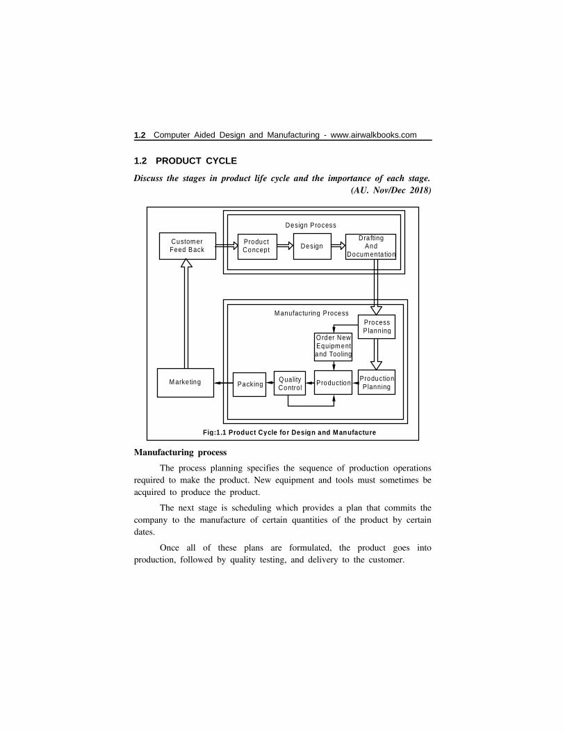
1.2 PRODUCT CYCLE

Discuss the stages in product life cycle and the importance of each stage.(AU. Nov/Dec 2018)

Manufacturing process

The process planning specifies the sequence of production operationsrequired to make the product. New equipment and tools must sometimes beacquired to produce the product.

The next stage is scheduling which provides a plan that commits thecompany to the manufacture of certain quantities of the product by certaindates.

Once all of these plans are formulated, the product goes intoproduction, followed by quality testing, and delivery to the customer.

Design Process

ProductConcept Design

Dra fting And

Docum enta tion

M anufacturing Process

Custom erFeed Back

M arke ting Packing

Order New Equipm entand Tooling

ProcessPlanning

Production ProductionPlanning

Fig:1.1 Product Cycle for Design and Manufacture

QualityControl

1.2 Computer Aided Design and Manufacturing - www.airwalkbooks.com

1.2.1 Typical product cycle

List the various activities involved in product development(AU. Nov/Dec 2018)

The impact of CAD/CAM involves in all the different activities of theproduct cycle, which is shown in Fig. 1.2.

Computer - aided design and automated drafting are utilized in theconceptualization, design, and documentation of the product. Computers areused in production to monitor and control the manufacturing operation. Inquality control, computers are used to perform inspections and performancetests on the product and its components.

Computer Aided design

Computer Autom atedDra fting and

Docum enta tion

ProductControl

DesignEngineering Dra fting

Custom ersand

M arkets

Order NewEquipm entand Too ling

ProcessPlanning

ComputerAided

ProcessPlanning

QualityControl

Production Scheduling

Computer Aided QualityControl

Computer Controlled

Robots, M ach ines, E tc

Computerized SchedulingM aterial Requ irement Planning , Shop Floor

Control

Fig:1.2 Product Cycle with CAD / CAM

www.srbooks.org Introduction 1.3

Design process

Fig. 1.1 shows the various steps involved in the product cycle. The productcycle is driven by customers and markets which demand the product. It is realisticto think of these as a large collection of diverse industrial and consumer marketsrather than one monolithic market. Depending on the particular customer groupthere will be differences in the way the product cycle is activated.

In some cases, the design functions are performed by the customer andthe product is manufactured by a different firm. In other cases, design andmanufacturing is accomplished by the same firm. But somehow, the productcycle begins with an idea of product or product concept.

This concept is generated, refined, analyzed, improved and translatedinto a plan for the product through the design engineering process. The planis documented by drafting a set of engineering drawings showing how theproduct is made and providing a set of specifications indicating how theproduct should perform.

With the engineering changes (i.e) drafting which typically follow theproduct throughout its life cycle this completes the design activities.

In the design and production operations of modern manufacturingtechniques, the computer has become a pervasive, useful and indispensable tool.It is strategically important and competitively imperative that manufacturing firmsand the people who are employed by them understand CAD/CAM.

1.3 DESIGN PROCESS

Describe various stages of design process with example.

(AU. Nov/Dec 2016)

Design process is an activity that facilitates the realization of newproducts and processes through which technology the human needs andaspirations are satisfied.

Design process cannot be summarized in a formula. It can be the workof an individual or efforts of a group of people. Design process is not straightforward but it is an iterative process. It means that after processing everystep of design process one should go to the previous steps.


There are many ways of defining the steps in a traditional designprocess. In 1975 Deutschman has summarized the design process in thefollowing nine steps.

iii(i) Recognition of need

ii(ii) Problem definition and specification

i(iii) Feasibility study

i(iv) Design synthesis

ii(v) Analysis and preliminary design

i(vi) Detailed design

i(vii) Prototype building and testing

(viii) Design for mass production

ii(ix) Product release

Recognition of N eeds

Problem D efinition

Synthesis

Analys is and O ptimization

Design Review

Presentation

M odification M odification

Fig: 1.3 Conventional Design Process


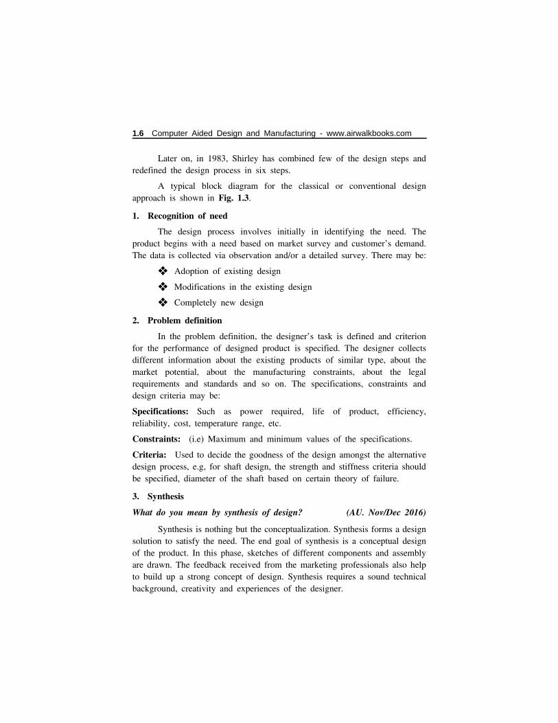
Later on, in 1983, Shirley has combined few of the design steps andredefined the design process in six steps.

A typical block diagram for the classical or conventional designapproach is shown in Fig. 1.3.

1. Recognition of need

The design process involves initially in identifying the need. Theproduct begins with a need based on market survey and customer’s demand.The data is collected via observation and/or a detailed survey. There may be:

❖ Adoption of existing design

❖ Modifications in the existing design

❖ Completely new design

2. Problem definition

In the problem definition, the designer’s task is defined and criterionfor the performance of designed product is specified. The designer collectsdifferent information about the existing products of similar type, about themarket potential, about the manufacturing constraints, about the legalrequirements and standards and so on. The specifications, constraints anddesign criteria may be:

Specifications: Such as power required, life of product, efficiency,reliability, cost, temperature range, etc.

Constraints: (i.e) Maximum and minimum values of the specifications.

Criteria: Used to decide the goodness of the design amongst the alternativedesign process, e.g, for shaft design, the strength and stiffness criteria shouldbe specified, diameter of the shaft based on certain theory of failure.

3. Synthesis

What do you mean by synthesis of design? (AU. Nov/Dec 2016)

Synthesis is nothing but the conceptualization. Synthesis forms a designsolution to satisfy the need. The end goal of synthesis is a conceptual designof the product. In this phase, sketches of different components and assemblyare drawn. The feedback received from the marketing professionals also helpto build up a strong concept of design. Synthesis requires a sound technicalbackground, creativity and experiences of the designer.


In synthesis, the design parameters are adjusted to get a perfect fit; iffit does not occur, the designer can change the specifications or sometimeseven modify the need specified in Recognition of need.

4. Analysis and optimization

Analysis must be followed for every synthesis. Analysis is a highlyiterative process and requires good mathematical knowledge. Analysis meanscritically examining an already existing or proposed design to judge thesuitability for the task that is to be performed by the designer. Analysisdetermines whether the performance complies with the requirements or not.The analysis subprocess selects suitable material and its associative mechanicalproperties. Calculations are performed to determine the size or parametersusing the physical laws such as laws of momentum, motion, energyconservation, etc. The different types of engineering analysis are stress-strainanalysis, kinematic analysis, dynamic analysis, vibration analysis, thermalanalysis, fluid-flow analysis, etc.

Optimization means the best possible solution for the given objectives.All possible solutions are analyzed and optimum is selected. After every phaseof design process, the designer may go to the previous steps and modifythem.

5. Design review

Design review is nothing but evaluation. Evaluation means measuringthe design against the specifications set in the problem definition. It usuallyinvolves prototype building and testing of the product to ascertain operatingperformance or factors such as reliability. The result of evaluation phase mayyield a satisfactory design or it may lead to further modifications in the designparameters. The changes into the prototype assembly are incorporated duringcontinued testing of the product. This process is repeated until satisfactoryperformance of the component and assembly is achieved.

6. Presentation

Presentation means drafting. The final stage in design process is thepresentation and documentation of the design on paper. This forms aninterface between the design and the manufacture.


Production drawing shows various design parameters, machiningparameters, tolerances etc. The design is presented using the drawings, partslist, materials, specifications, etc. The design is not complete if one cannotsell it. Therefore a great deal of effort should be applied in the presentationof the design.

1.4 SEQUENTIAL ENGINEERING

The conventional product cycle is sequential. It contains quality control,product design, manufacturing process with every activity is carried out in asequential manner.

In sequential engineering, each department is insulated i.e. eachdepartment functions separately.

There is no interaction among the groups.

This is time consuming as for example, if any flaw is encounteredduring the quality check stage, the product has to go through the whole cyclefrom the start.

Design P lanning M anufactu ring Q ua lity M arke ting

Fig:1.4 Sequential Engineering


1.5 CONCURRENT ENGINEERING

Discuss the significance of concurrent engineering approach in limitingdesign changes. (AU. Nov/Dec 2018)

Concurrent engineering is known as simultaneous engineering. Here,while the product is designed, the design and manufacturing processes arecarried out simultaneously. This technique facilitates the design engineer toimprove the efficiency of product design and process. This is effectiveinteraction of process planning and product design. Concurrent engineeringalso influences the cycle cost of product. Concurrent engineering also unitespeople from different functional areas.

The block diagram of concurrent engineering is shown in Fig.1.5.

In a traditional designing process, complete design descriptions areproduced in the form of engineering drawings and diagrams and these arethen issued by the design department of a company for analytical evaluation,and for the preparation of plans and instructions for manufacture. Inevitably,the manufacturing specialists and design analyst find aspects of the designthat should be improved, and so the design is returned to the designdepartment for modification and reissue of the drawings.

Inspection

M anufacturing

Function

M arke ting

DesignCo-ord inator

Fig:1.5 Sim ultaneous (or) Concurrent Engineering

Serv ic ib ility Sa les

Assem bly Packaging


In some cases reissue may occur many times - one large aerospacemanufacturer is said to change each drawing an average of 4.5 times beforefinal release - and thus the whole process is both time consuming and costly.

Furthermore because the considerations of manufacturing and otherspecialists are taken into account after the design drawings have beenproduced, the design department tends to concentrate on functional aspects ofthe design at the expense of ease of manufacture, maintainability and so on.

Concurrent engineering aims to overcome all of these limitations, bybringing together a design team with the appropriate combination of specialistexpertise to consider early in the design process, all elements of the productlife cycle from conception through manufacture and use in service tomaintenance and disposal.

1.5.1 Characteristics of concurrent engineering

❖ Constant and un-interrupted evaluation of design process anddevelopment process.

❖ Fast and speedy information exchange achieved through internet,LAN etc.

❖ Rapid prototyping.

❖ More attention and concern for satisfying customer needs.

❖ Focus on new technologies.

1.5.2 Need for implementation of concurrent engineering

❖ In order to effectively implement concurrent engineering, suitabletraining programs need to be organized.

❖ The power should be decentralized which allows effectiveparticipation of workers from all levels to work together and solvethe problem.

❖ Concurrent engineering ensures that the problem between designand manufacturing, design and production, etc. are removed.

❖ In concurrent engineering there is simultaneous interaction betweenthe groups, moreover all the procedures are split into simple taskswhich are easier to complete.


1.6 COMPARISON OF SEQUENTIAL AND CONCURRENT ENGINEERING

Compare and contrast sequential and concurrent engineering with suitableexamples. (AU. Apr/May 2017)

Sequential engineering is followed in conventional manufacturing. Asmentioned earlier, this process flows in one direction and back-tracking atany stage is time consuming and has to be started from first step. Moreover,the activities of each department is localised and isolated. Thus interactionamong the group is lacking.

On the other hand, concurrent engineering facilitates an effectiveinteraction between various departments, such as production planning,production development and manufacturing. Thus the spirit of team work isdeveloped. Moreover specialists from different departments interact with eachother and improve the efficiency of the production design. Concurrentengineering includes special methods such as DFMA (Design formanufacturing and assembly) and FMEA (Failure mode and effect analysis)for flaw finding and design optimizing.

Another difference is, in the infant stages numerous changes will beencountered in the product cycle and these changes progressively come downfor the rest (i.e.) remaining period for concurrent engineering.

In case of sequential engineering changes may not be constant andpredicted, but the magnitude of change differ at every stage.

This comparison is depicted in the Fig. 1.6.

Concurren t Eng ineering

Sequential Engineering

Product Development C ycle

Nu

mbe

r of

Ch

ange

Fig:1.6 Com parison Graph


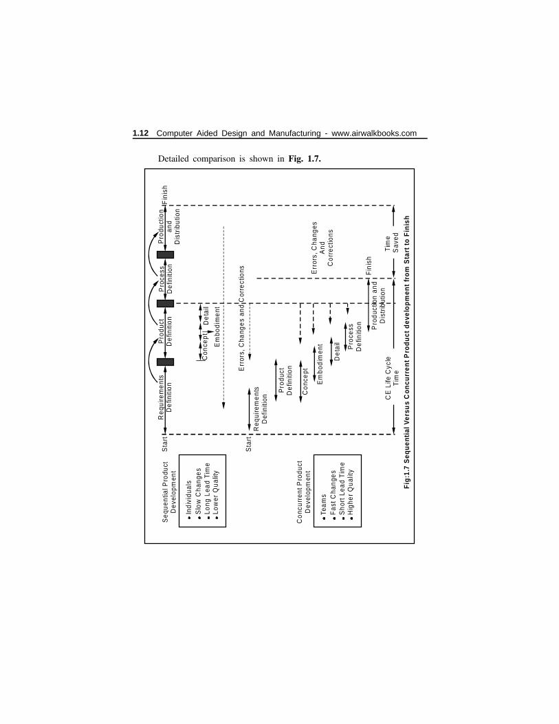
Detailed comparison is shown in Fig. 1.7.R

equ

irem

ent

sD

efin

itio

nP

rodu

ct

De

finiti

onP

roce

ssD

efin

ition

Pro

duct

ion

and

D

istr

ibut

ion

Fin

ish

Sta

rt

Sta

rt

Con

cep

tD

eta

il

Em

bodi

me

nt

Err

ors,

Cha

nge

s an

d C

orre

ctio

ns Err

ors,

Cha

nges

A

nd

Co

rrec

tions

Fin

ish

Req

uire

me

nts

Def

initi

on

Pro

duct

D

efin

ition

Co

nce

pt

Em

bod

imen

t

De

tail Pro

cess

De

finiti

on

Pro

duc

tion

and

D

istr

ibut

ion

CE

Life

Cyc

le

Tim

eT

ime

Sav

ed

Se

quen

tial P

rodu

ctD

evel

opm

ent

Ind

ivid

uals

S

low

Cha

nge

s Lo

ng L

ead

Tim

e Lo

wer

Qua

lity

Tea

ms

Fas

t Cha

nge

s S

hor

t Le

ad

Tim

e H

ighe

r Q

ual

ity

Co

ncu

rren

t Pro

duct

Dev

elop

men

t

Fig

:1.7

Seq

uen

tial

Ver

sus

Co

ncu

rren

t P

rod

uct

dev

elo

pm

ent

fro

m S

tart

to

Fin

ish


1.7 COMPUTER AIDED DESIGN

In the field of computer science and technology the advancements haveresulted in the emergence of very powerful hardware and software tools thatoffer scope in the conventional design process, which results in theimprovement of quality of the product.

Thus, Computer aided design is the automation of design process.

CAD is the use of computer to aid in the design process of anindividual part, a subsystem or total system.

CAD is the process of creation and development of a prototype on acomputer to assist the engineer in the design process.

CAD creates a three dimensional geometric model on the computer toexamine the geometric and manufacturing requirements of an object.

1.7.1 Why should we go for CAD?

There are four fundamental reasons for implementing the CAD system,which are as follows.

(i) To increase the productivity of the designer.

(ii) To improve the quality of the design.

(iii) To improve communications.

(iv) To create a database for engineering.

1. To increase the productivity of the designer

The product and its components, subassemblies and parts can bevisualised quickly by the designer using CAD. Time for synthesis, analysisand documentation of the design will be reduced. Even it reduces design timeand cost.

2. To improve the quality of design

Without any error, quick alterations can be made in the design withthe help of CAD.

3. To improve communications

Better documentation of the design, fewer drawing errors with greaterlegibility will be provided by CAD.


4. To create database for engineering

The product geometries and dimensions, bill of materials, etc., will makea design database, which are essential input for manufacturing of the product.

1.7.2 Factors considered for selecting CAD system

(a) Reliability

(b) Compatibility with other systems

(c) Cost factors

(d) Memory size and storage requirement.

(e) Type of peripherals required.

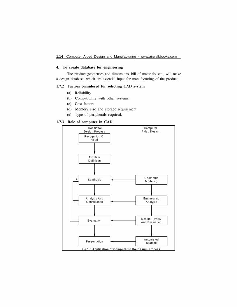
1.7.3 Role of computer in CAD

TraditionalD esign Process

C om puterA ided D es ign

R ecogn it ion O f N eed

ProblemD efin ition

Synthes is

Analys is A nd O ptim iza tion

Evalua tion

P resen tation

G eom etric M odeling

EngineeringAnalys is

D esign Review And Evalua tion

Au tomatedD ra fting

Fig:1.8 Application of Computer to the Design Process


(i) Computer improves accuracy of design.

(ii) Various dimensions, and other design attributes can be convenientlymanipulated by computers.

(iii) Another role played by computers is creation of part libraries forstandard components. Similarly multiple components can be includedin these part libraries.

(iv) Moreover the modification of the model is very simple which helpsthe designer to look in for further improvement.

(v) Calculation of various geometric properties such as area, volume,and dimenioning can be accurately done.

The application of computers to the designing process is shown in Fig. 1.8.

1.8 BENEFITS OF CAD

State any two benefits of CAD (AU. Apr/May 2017)

Some important benefits of CAD are:

❖ CAD is faster, consistent and more accurate than the classicaldesign process.

❖ The manipulation of various dimensions, attributes is easilypossible under the CAD environment. Some CAD software isparametric and possesses parent-child relationship between thecomponent and assembly.

❖ The efficiency, effectiveness and creativity of the designer improvedrastically, leading to high quality engineering designs. The addedadvantage of CAD is excellent graphical representation andproduction drawing of product with exchange facility betweendifferent phases through e-drawing.

❖ Easy modification and improvement of product is possible in CADenvironment taking care of further needs.

❖ In CAD, it is not required to repeat the design or drawing of anycomponent with modified dimensions. It is possible to copy andmodify the designs as per the new dimension within seconds,including geometric transformations, material replacements, ifneeded.


❖ Graphics simulation and animation makes it possible to study thereal-time behaviour of CAD assembly. This is useful for inspectingtolerance and interface between the matching components of themodel.

❖ Use of standard components in part libraries makes very fast CADmodeling. For a specific task, various components, subassemblymay be stored in part libraries for future use.

❖ 3D visualization of model from several orientations eliminates theneed of making a prototype.

❖ The documentation at various design phases is efficient, easier,flexible and economical. The coordination among the groups andsharing of design data and results is possible in CAD environment.

❖ Most CAD software can link the geometric model directly to itsmanufacturing counterpart, i.e, CAM to carry out production.

1.9 ENGINEERING APPLICATIONS OF CAD

Mention any four applications of computer aided design in mechanicalengineering? (AU. Nov/Dec 2015)

The CAD system is extensively used in mechanical engineering andmanufacturing industries. CAD increases productivity of designer through thevisualization of components/assemblies. The engineering applications ofcomputer aided design (CAD) are shown in Table 1.1.

Table: 1.1 - Applications of CAD

S.No. Applications Detail

1. Structural design ofAircraft

CAD analyzes the turbulent flow pattern inaerospace structures

2. Aircraft simulation The complex situation during the flight canbe simulated in flight simulator using theCAD software, which avoids lengthy delay,saves fuel cost and provides better thanpilots.


S.No. Applications Detail

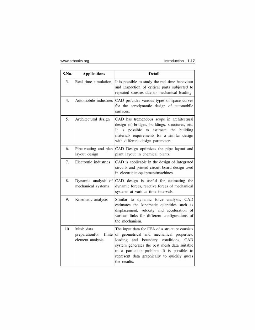
3. Real time simulation It is possible to study the real-time behaviourand inspection of critical parts subjected torepeated stresses due to mechanical loading.

4. Automobile industries CAD provides various types of space curvesfor the aerodynamic design of automobilesurfaces.

5. Architectural design CAD has tremendous scope in architecturaldesign of bridges, buildings, structures, etc.It is possible to estimate the buildingmaterials requirements for a similar designwith different design parameters.

6. Pipe routing and planlayout design

CAD Design optimizes the pipe layout andplant layout in chemical plants.

7. Electronic industries CAD is applicable in the design of Integratedcircuits and printed circuit board design usedin electronic equipment/machines.

8. Dynamic analysis ofmechanical systems

CAD design is useful for estimating thedynamic forces, reactive forces of mechanicalsystems at various time intervals.

9. Kinematic analysis Similar to dynamic force analysis, CADestimates the kinematic quantities such asdisplacement, velocity and acceleration ofvarious links for different configurations ofthe mechanism.

10. Mesh datapreparationfor finiteelement analysis

The input data for FEA of a structure consistsof geometrical and mechanical properties,loading and boundary conditions, CADsystem generates the best mesh data suitableto a particular problem. It is possible torepresent data graphically to quickly guessthe results.


So far, CAD systems have been described in very general terms. Morespecifically, they can be thought of as comprising:

❖ Hardware:

The computer and associated peripheral equipment.

❖ Software:

The computer program(s) running on the hardware.

❖ Data:

The data structure created and manipulated by the software.

CAD systems are no more than computer programs perhaps usingspecialized computing hardware. The software normally comprises a numberof different elements or functions that process the data stored in the databasein different ways. These are represented diagrammatically in Fig. 1.9 andinclude elements for:

❖ Model definition:

For example, to add geometric elements to a model of the form of acomponent.

Data Functions

Database

Input

Outpu tUser

M odelDefin it ion

M anipulation

PictureGeneration

Utilities

Data BaseM anagement

Applications

Fig:1.9 The Architecture of Computer Aided D esign System

ComponentM odels

Drawings

Standards

L ib raryData

W orking Data

Geom etry

Associated Data

M anufacturing


❖ Model manipulation:

To move, copy, delete, edit or otherwise modify elements in the designmodel.

❖ Picture generation:

The generate images of the design model on a computer screen or onsome hard-copy device.

❖ User interaction:

To handle commands input by the user and to present output to theuser about the operation of the system.

❖ Database management:

For the management of files that makeup the database.

❖ Applications:

These elements of the software don’t modify the design model, butuse it to generate information for valuation, analysis or manufacture.

❖ Utilities:

Parts of the software that do not directly affect the design model, butmodify the operation of the system in some way.

For example, To select the colour to be used for display, or the unitsto be used for construction of a part model.

These features may be provided by multiple programs operating on acommon database or by a single program encompassing all of the elements.

1.10 COMPUTER GRAPHICS

❖ Computer graphics is the language of engineers, which provides apowerful tool for communication among the team membersassociated with design, manufacturing and sales of a product.

❖ Computer graphics involves the creation, storage, manipulation andintegration of models and images of the object by means of adigital computer.

The shaded and coloured two-dimensional, three-dimensional andhigher-dimensional models are generated to bring the realism in different


objects such as natural scene, animation, flight simulation, navigation,commerce, advertising, etc.

In recent years, computer graphics become a very powerful tool for thedevelopment of high quality pictures rapidly, consistently and economically.

Computer graphics is an important tool in computer aidedmanufacturing (CAM) where the graphical data of the object, converted intomachine data, operates CNC machines for production.

The synthesis of real or imaginary objects from their computer modelis concerned by computer graphics.

The image processing is the reverse of computer graphics, whichperforms the analysis of pictures.

The computer graphics and image processing techniques together dealwith the computer processing of pictures. Both use raster displays, combinedin interactive image processing.

Computer graphics is very popular in industries, business, education,medicine, fashion, entertainment, etc.

It has made things easier to visualize.

1.11 COORDINATE REPRESENTATION SYSTEM

Every CAD/CAM system follows certain type of coordinaterepresentation system. While displaying an image, the mapping of coordinatesof the object consisting of 2D and 3D primitives occurs onto the displaydevice or workstation. This is obtained through the coordinatestransformations, also referred to as viewing transformations.

1.11.1 Cartesian coordinate system

Cartesian coordinate system is mostly followed by the graphicssoftware design. If coordinates of an image is defined in other coordinatesystem (eg., cylindrical or spherical coordinate system), they must beconverted into the cartesian coordinates before using in the graphics software.

Fig. 1.10 shows the viewing transformation sequence from localcoordinates to the device coordinates. Broadly, three types of coordinatesystem are required to input display and store the geometry of graphics modelduring the modeling process.


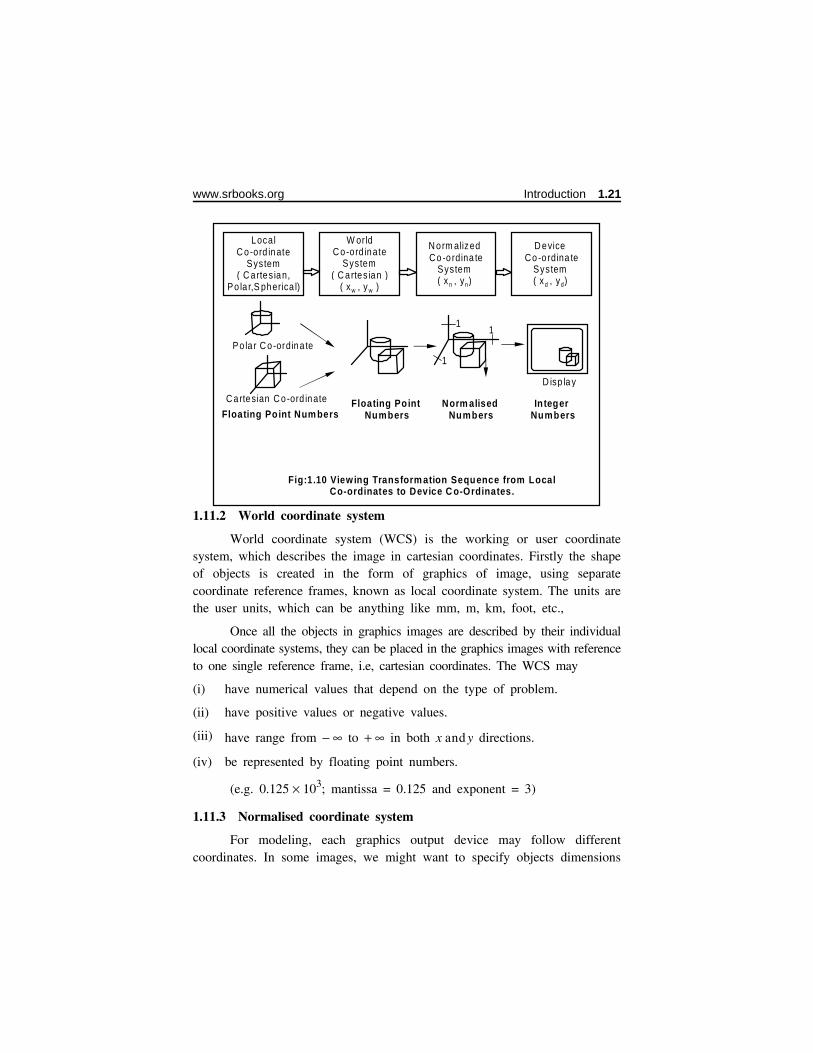
1.11.2 World coordinate system

World coordinate system (WCS) is the working or user coordinatesystem, which describes the image in cartesian coordinates. Firstly the shapeof objects is created in the form of graphics of image, using separatecoordinate reference frames, known as local coordinate system. The units arethe user units, which can be anything like mm, m, km, foot, etc.,

Once all the objects in graphics images are described by their individuallocal coordinate systems, they can be placed in the graphics images with referenceto one single reference frame, i.e, cartesian coordinates. The WCS may

(i) have numerical values that depend on the type of problem.

(ii) have positive values or negative values.

(iii) have range from − ∞ to + ∞ in both x and y directions.

(iv) be represented by floating point numbers.

(e.g. 0.125 × 103; mantissa = 0.125 and exponent = 3)

1.11.3 Normalised coordinate system

For modeling, each graphics output device may follow differentcoordinates. In some images, we might want to specify objects dimensions

Po la r C o-ordina te

C artesian C o-ord inate

Local C o-ord inate

System( C artes ian,

Po la r,S pherica l)

W orld C o-ord inate

System( C artes ian )

( x , y )w w

N orm alized Co -o rdina te

System( x , y )n n

D evice Co -o rdina te

System( x , y )d d

Fig:1.10 Viewing Transform ation Sequence from Local Co-ordinates to Device C o-Ordinates.

Floating Point Num bersFloating Point

NumbersNorm alised Numbers

Integer Numbers

11

1

D isp la y


in fraction of a foot, while for some other applications it may be ‘mm’ (or)‘km’.

It is, therefore, desirable to convert the world coordinates into thenormalized coordinates. i.e, Normalized coordinate system (NCS), to makethe coordinate system independent of several graphics output devices.

Normalization may be done from (0,0) to (1,1) with origin at (0,0) inthe lower left corner and co-ordinate (1,1) on the right top corner of thedisplay devices.

To accommodate the differences in scales and aspect ratios, themapping of normalized coordinates into square area of the displays is requiredto maintain the proper proportions of various images.

1.11.4 Device coordinate system

The device coordinate system is one in which the image of normalizedcoordinate system will be displaced in the output device like monitor (softdevice), printer/plotter (hard device).

A graphics device understands the device coordinate system in termsof pixels, cm, inch, etc.

Depending upon the pixel density, the DCS would vary from onesystem to another.

The features of device control system are follows:

(i) The pixel density (eg: 1024 × 1024) of the display device dependson the maximum size.

(ii) Positive values have to be considered.

(iii) Always fixed in size (i.e. size of display surface) irrespective of theproblem.

(iv) It should be always represented by an integer number.


1.12 TWO DIMENSIONAL TRANSFORMATION

Basic transformation

Explain the different types of 2D transformation with examples.(AU. Nov/Dec 2017)

List and differentiate the types of 2D geometric transformations.

Explain the various graphic transformation required for manipulating thegeometric information. (AU. Apr/May 2018)

The transformations are used to reposition and resize two-dimensionalobjects on the displays (alternatively, in the database).

The three basic transformations are as follows:

(i) Translation

(ii) Scaling

(iii) Rotation

Any point is represented by its coordinates (x, y, z) from the referencedatum in the three dimensional system. For simplicity and to make it easyto understand, we can analyse the two dimensional system. Then we candiscuss the 3D system.

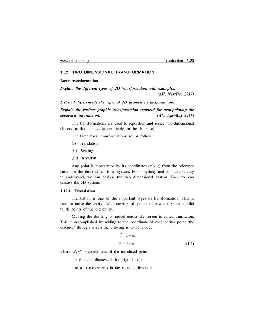
1.12.1 Translation

Translation is one of the important types of transformation. This isused to move the entity. After moving, all points of new entity are parallelto all points of the old entity.

Moving the drawing or model across the screen is called translation.This is accomplished by adding to the coordinate of each corner point ‘thedistance’ through which the drawing is to be moved

x′ = x + m

y′ = y + n ...(1.1)

where, x′, y′ → coordinates of the translated point

x, y → coordinates of the original point

m, n → movements in the x and y direction


In matrix notation this can be represented as

(x′, y′) = (x, y) + T ...(1.2)

where,

T = (m, n), the translation matrix

Problem 1.1: Translate a two dimensional rectangle as shown in figure, byadding 4 units in x - coordinate and 3 units in y - coordinate.

Given data

T = (4, 3)

x1 = 1; y1 = 1

x2 = 4; y2 = 1

x3 = 4; y3 = 5

x4 = 1; y4 = 5

To find

New translated rectangle

Solution

From equation (1.2)

We know that

(x′, y′) = (x, y) + T ...(1)

Expanding the equation (1) for 4 coordinate rectangle

⎧

⎨

⎩

⎪⎪

⎪⎪

x1′x2′x3′xr′

y1′y2′y3′y4′

⎫

⎬

⎭

⎪⎪

⎪⎪

=

⎡

⎢

⎣

⎢⎢⎢⎢

x1x2x3x4

y1y2y3y4

⎤

⎥

⎦

⎥⎥⎥⎥

+ [T]

Substitute the given data values in equation (2), then we have ...(2)

( 1 ,5 ) ( 4 ,5 )

( 4 ,1 )( 1 ,1 )

Fig.


⎧

⎨

⎩

⎪⎪

⎪⎪

x1′x2′x3′x4′

y1′y2′y3′y4′

⎫

⎬

⎭

⎪⎪

⎪⎪

=

⎡

⎢

⎣

⎢

⎢

1441

1155

⎤

⎥

⎦

⎥

⎥ + [4 3]

⎧

⎨

⎩

⎪⎪

⎪⎪

x1′x2′x3′x4′

y1′y2′y3′y4′

⎫

⎬

⎭

⎪⎪

⎪⎪

=

⎡

⎢

⎣

⎢

⎢

5885

4488

⎤

⎥

⎦

⎥

⎥...(3)

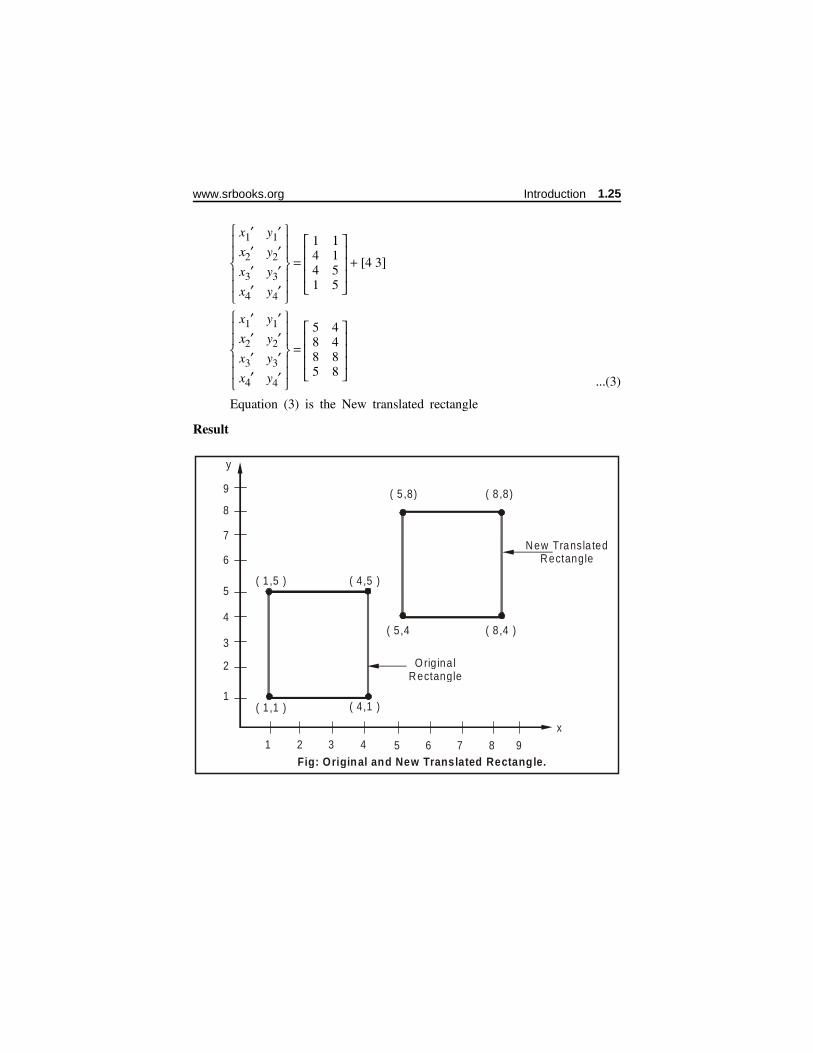
Equation (3) is the New translated rectangle

Result

( 1 ,5 ) ( 4 ,5 )

( 4 ,1 )( 1 ,1 )

( 5 ,4 ( 8 ,4 )

( 8 ,8)( 5 ,8)

O rig ina lRectangle

New Transla tedRectangle

y

x

9

8

7

6

5

4

3

2

1

1 2 3 4 5 6 7 8 9Fig: Original and New Translated Rectangle.


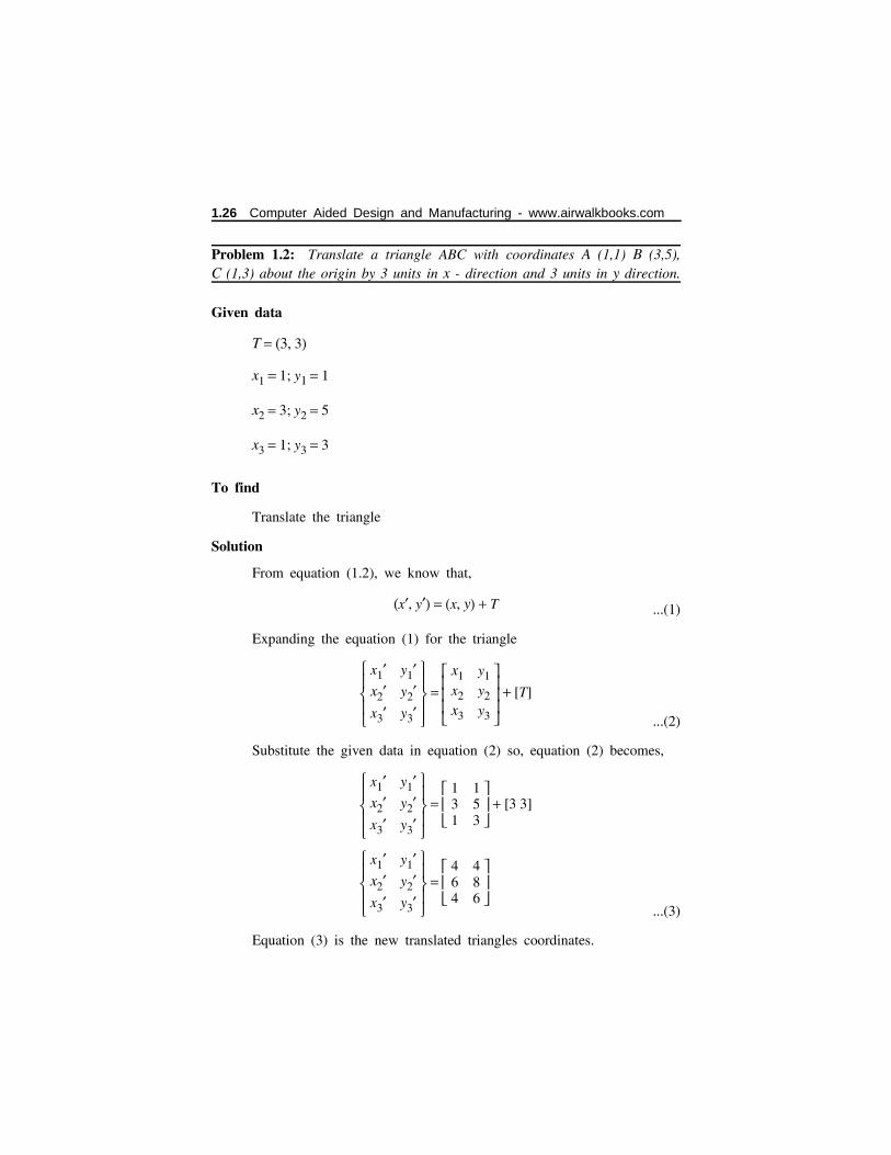
Problem 1.2: Translate a triangle ABC with coordinates A (1,1) B (3,5),C (1,3) about the origin by 3 units in x - direction and 3 units in y direction.

Given data

T = (3, 3)

x1 = 1; y1 = 1

x2 = 3; y2 = 5

x3 = 1; y3 = 3

To find

Translate the triangle

Solution

From equation (1.2), we know that,

(x′, y′) = (x, y) + T ...(1)

Expanding the equation (1) for the triangle

⎧

⎨

⎩

⎪

⎪

x1′x2′x3′

y1′y2′y3′

⎫

⎬

⎭

⎪

⎪ =

⎡

⎢

⎣

⎢

⎢

x1x2x3

y1y2y3

⎤

⎥

⎦

⎥

⎥ + [T]

...(2)

Substitute the given data in equation (2) so, equation (2) becomes,

⎧

⎨

⎩

⎪

⎪

x1′x2′x3′

y1′y2′y3′

⎫

⎬

⎭

⎪

⎪ =

⎡⎢⎣ 131

153 ⎤⎥⎦ + [3 3]

⎧

⎨

⎩

⎪

⎪

x1′x2′x3′

y1′y2′y3′

⎫

⎬

⎭

⎪

⎪ =

⎡⎢⎣ 464

486 ⎤⎥⎦

...(3)

Equation (3) is the new translated triangles coordinates.


Result

Problem 1.3: Consider the line defined by, L = ⎡⎢⎣ 13

24 ⎤⎥⎦. Translate the line

3 units in x - direction and 4 units in y direction.

Given data

T = (3, 4)

x1 = 1; y1 = 2

x2 = 3; y2 = 4

To find

Translate the line

Solution

From equation 1.2 we get,

(x′, y′) = (x, y) + T ...(1)

O rig in a lTriangle

TranslatedTriangle

y

x

8

7

6

5

4

3

2

1

1 2 3 4 5 6 7 8

Fig: O riginal and New Translated Triangle

( 1 ,1 )

( 3 ,5 )

( 1 ,3 ) ( 4 ,4 )

( 4 ,6 )

( 6 ,8 )


Expand the equation (1) for 2 points. So equation (1) becomes,

⎡⎢⎣ x1′x2′

y1′y2′

⎤⎥⎦ =

⎡⎢⎣ x1x2

y1y2

⎤⎥⎦ + [T]

...(2)

Substitute the given data in equation (2)

⎡⎢⎣ x1′x2′

y1′y2′

⎤⎥⎦ = ⎡⎢

⎣ 13 2

4 ⎤⎥⎦ + [3 4]

⎡⎢⎣ x1′

x2′

y1′

y12

⎤⎥⎦ = ⎡⎢

⎣ 46 6

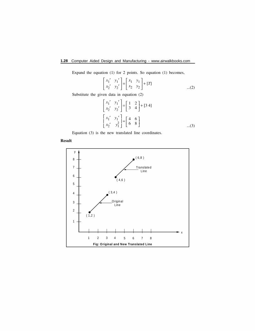
8 ⎤⎥⎦ ...(3)

Equation (3) is the new translated line coordinates.

Result

y

x

8

7

6

5

4

3

2

1

1 2 3 4 5 6 7 8

Fig: Original and New Translated Line

Orig inalL ine

Translated L ine

( 1,2 )

( 3,4 )

( 4,6 )

( 6,8 )


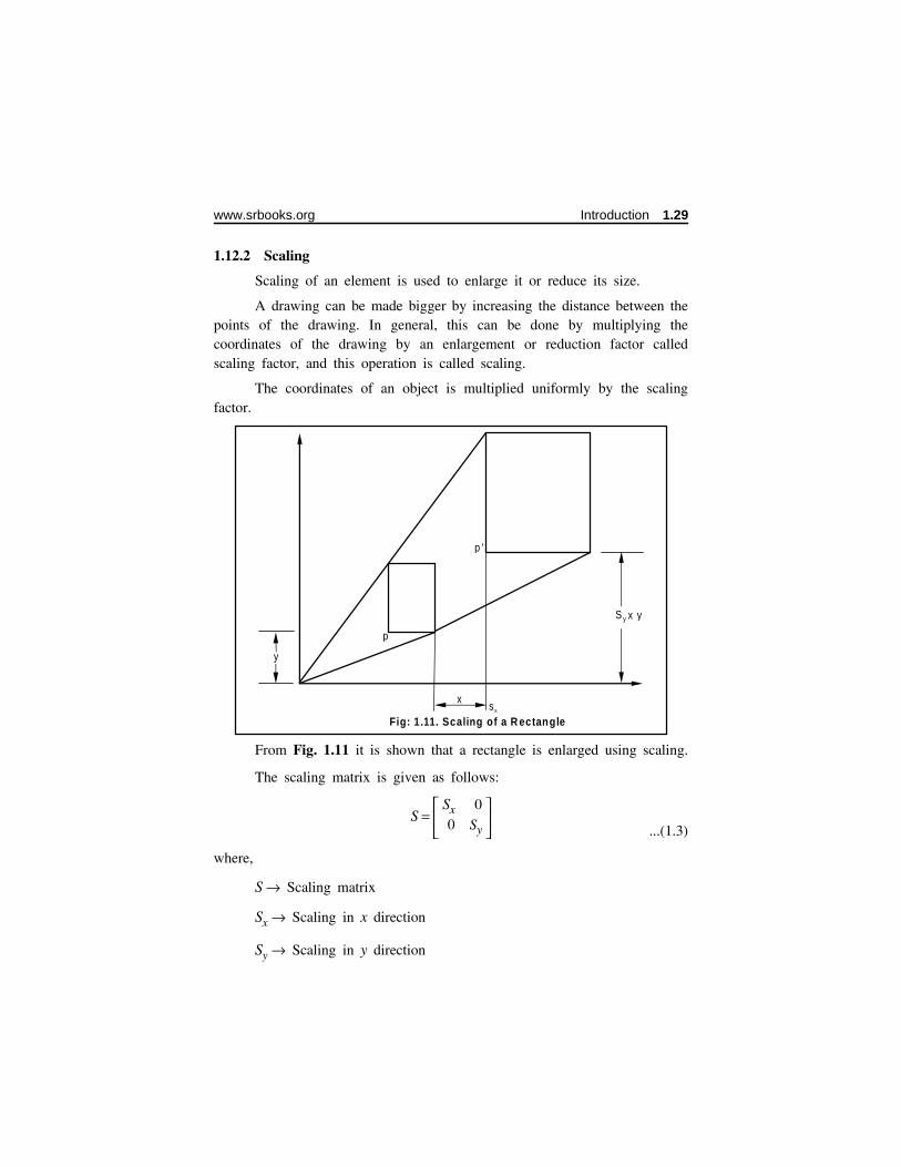
1.12.2 Scaling

Scaling of an element is used to enlarge it or reduce its size.

A drawing can be made bigger by increasing the distance between thepoints of the drawing. In general, this can be done by multiplying thecoordinates of the drawing by an enlargement or reduction factor calledscaling factor, and this operation is called scaling.

The coordinates of an object is multiplied uniformly by the scalingfactor.

From Fig. 1.11 it is shown that a rectangle is enlarged using scaling.

The scaling matrix is given as follows:

S = ⎡⎢⎣ Sx0

0

Sy ⎤⎥⎦ ...(1.3)

where,

S → Scaling matrix

Sx → Scaling in x direction

Sy → Scaling in y direction

y

p

p ’

S y

Fig: 1.11. Scaling of a R ectangle

x y

xsx


Sx and Sy need not be equal. A circle can be transformed into an

ellipse by unequal scaling factors Sx and Sy. If the scaling factors are less

than 1, it will reduce the size of the object and the object is moved towardsthe origin.

If it is greater than 1, then it will enlarge the size of the object andobject is moved away from the origin.

P′ = [x′, y′] = [Sx × x, Sy × y]

The above equation can be represented in a matrix form as follows:

P′ = ⎡⎢⎣ Sx0

0Sy

⎤⎥⎦ ⎡⎢⎣ xy ⎤⎥⎦ ...(1.4)

(i.e)

P′ = [S] ⋅ [P]

❖ While zooming or magnifying the object, uniform scaling ((i.e)

Sx = Sy) is applied.

❖ Zooming or magnifying is only a display attribute and is used onlyto the display and not stored in actual geometric database.

Problem 1.4: A line AB ⎡⎢⎣ 13

24 ⎤⎥⎦ is enlarged by a scaling factor of 2. Show

the transformation.

Given data

Sx = Sy = 2

x1 = 1 ; y1 = 2

x2 = 3 ; y2 = 4

To find

To obtain the transformation using scaling.

Solution

The scaling matrix , S = ⎡⎢⎣ Sx0

0Sy

⎤⎥⎦


Original line matrix = AB = ⎡⎢⎣ 13

24 ⎤⎥⎦

Scaled line matrix is determined as follows.

[S] ⋅ [AB] = [A′ B′]

⎡⎢⎣ 20

02 ⎤⎥⎦ ⎡⎢⎣ 13

24

⎤⎥⎦ = [A′ B′]

A′ B′ = ⎡⎢⎣ 26 4

8 ⎤⎥⎦ → are new scaled line coordinates

Results

1.12.3 Rotation

Rotation is also an another important transformation. In thistransformation, all the points of an object are rotated about the origin (or)

about any base point by an angle θ.

For a positive angle, the object is rotated in anticlockwise directionand viceversa.

9

y

(6 ,8)

New sca led L ine

(3 ,4)

O rig ina lL ine

(1 ,2)

(2 ,4)

8

7

6

5

4

3

2

1 2 3 4 5 6 7 8 9x

1


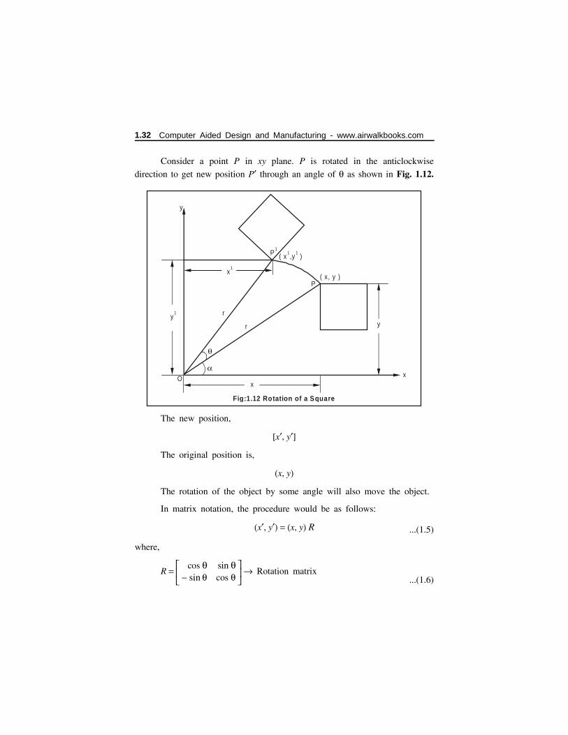
Consider a point P in xy plane. P is rotated in the anticlockwise

direction to get new position P′ through an angle of θ as shown in Fig. 1.12.

The new position,

[x′, y′]

The original position is,

(x, y)

The rotation of the object by some angle will also move the object.

In matrix notation, the procedure would be as follows:

(x′, y′) = (x, y) R ...(1.5)

where,

R = ⎡⎢⎣

cos θ− sin θ

sin θcos θ

⎤⎥⎦ → Rotation matrix

...(1.6)

y

x

y

x

y1

x1

r

r

P

O

P1

( x ,y )1 1

( x, y )

θ

α

Fig:1.12 Rotation of a Square


Problem 1.5: Consider the line of coordinates (1,1) and (2,4) Rotate the

line about the origin by 30°. Determine the transformation of the line.

Given data

θ = 30°

x1 = 1; y1 = 1

x2 = 2; y2 = 4

To find

Transformation of the line

Solution

We know that from equation (1.5)

x′ y′ = (x, y) R ...(1)

where,

R = ⎡⎢⎣

cos θ− sin θ

sin θcos θ

⎤⎥⎦ ...(2)

Apply θ as 30° in equation (2)

R = ⎡⎢⎣

cos 30°− sin 30°

sin 30°cos 30°

⎤⎥⎦

R = ⎡⎢⎣

0.866− 0.500

0.5000.866

⎤⎥⎦ ...(3)

Apply equation (3) in (1)

x′ y′ = ⎡⎢⎣ 12 1

4 ⎤⎥⎦ ⎡⎢⎣

0.866− 0.500

0.5000.866

⎤⎥⎦

x′ y′ = ⎡⎢⎣

0.366− 0.268

1.3664.464

⎤⎥⎦

The effect of applying the rotation matrix to the line is shown in result.


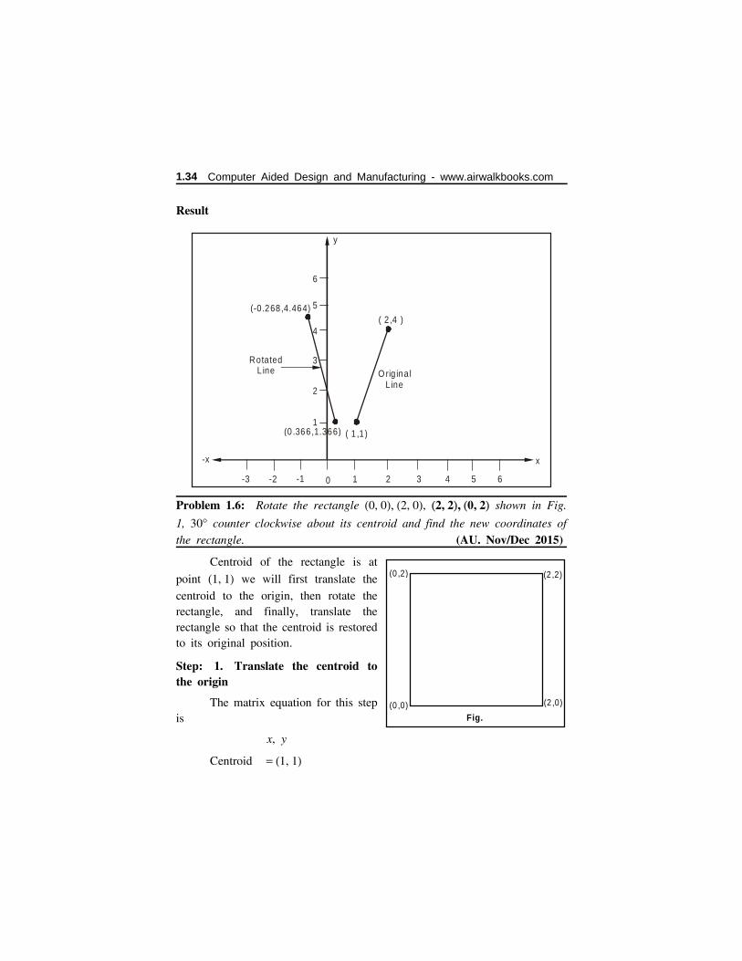
Result

Problem 1.6: Rotate the rectangle (0, 0), (2, 0), (2, 2), (0, 2) shown in Fig.

1, 30° counter clockwise about its centroid and find the new coordinates ofthe rectangle. (AU. Nov/Dec 2015)

Centroid of the rectangle is at

point (1, 1) we will first translate thecentroid to the origin, then rotate therectangle, and finally, translate therectangle so that the centroid is restoredto its original position.

Step: 1. Translate the centroid tothe origin

The matrix equation for this stepis

x, y

Centroid = (1, 1)

-x

0

1

2 3 4 5 6

2

3

4

5

1-2 -1-3

6

x

y

( 2 ,4 )

( 1 ,1 )(0 .366 ,1.366)

(-0.268 ,4.464)

RotatedL ine O rig ina l

L ine

(2 ,2)

(0 ,0) (2 ,0)

(0 ,2)

Fig.


[P∗]1 = [P] [Tt]

where [P] =

⎛

⎜

⎝

⎜

⎜

0220

0022

0000

1111

⎞

⎟

⎠

⎟

⎟

and [Tt] =

⎛

⎜

⎝

⎜⎜⎜⎜

100

− 1

010

− 1

0010

0001

⎞

⎟

⎠

⎟⎟⎟⎟

where [Tt] =

⎛

⎜

⎝

⎜⎜⎜⎜

100

− x

010

− y

0010

0000

⎞

⎟

⎠

⎟⎟⎟⎟

Step: 2. Rotate the Rectangle 30° counter clockwise about the z-axis.

The matrix equation for this step is given as

[P∗]2 = [P1∗] [Tr]θ

where, [P∗]1 is the resultant points matrix obtained in step 1, and [Tr] is the

rotation transformation, where θ = 30°

The Transformation matrix is

[Tr]θ =

⎛

⎜

⎝

⎜⎜⎜⎜

cos θ− sin θ

00

sin θcos θ

00

0010

0001

⎞

⎟

⎠

⎟⎟⎟⎟

=

⎛

⎜

⎝

⎜⎜⎜⎜

cos 30− sin 30

00

sin 30cos 30

00

0010

0001

⎞

⎟

⎠

⎟⎟⎟⎟

=

⎛

⎜

⎝

⎜⎜⎜⎜

0.866− 0.5

00

0.50.866

00

0010

0001

⎞

⎟

⎠

⎟⎟⎟⎟

Step: 3. Translate the Rectangle so that the centroid lies at its originalposition.

[P∗]3 = [P∗]2[T− t] ,


where [T− t] is the reverse translation matrix, given as

[T− t] =

⎛

⎜

⎝

⎜

⎜

1000

0100

0010

0001

⎞

⎟

⎠

⎟

⎟ , where [T− t] =

⎛

⎜

⎝

⎜

⎜

100x

010y

0010

0000

⎞

⎟

⎠

⎟

⎟

Now we can write the entire matrix equation that combines all thethree steps outlined above the equations is,

[P∗] = [P] [Tt] [Tr] [T− t]

Substituting the values, we get

[P∗] =

⎛

⎜

⎝

⎜

⎜

0220

0022

0000

1111

⎞

⎟

⎠

⎟

⎟ ×

⎛

⎜

⎝

⎜⎜⎜⎜

100

− 1

010

− 1

0010

0001

⎞

⎟

⎠

⎟⎟⎟⎟

×

⎛

⎜

⎝

⎜⎜⎜⎜

cos 30°− sin 30°

01

sin 30°cos 30°

01

0010

0001

⎞

⎟

⎠

⎟⎟⎟⎟

×

⎛

⎜

⎝

⎜

⎜

1000

0100

0010

0001

⎞

⎟

⎠

⎟

⎟

=

⎛

⎜

⎝

⎜⎜⎜⎜

0.6340− 0.3660

1.3660− 0.3660

− 0.36601.36602.36601.3660

0000

1111

⎞

⎟

⎠

⎟⎟⎟⎟

The first two column represent the new coordinates of the rotatedrectangle.

Problem 1.7: Given the triangle, described by the homogeneous pointsmatrix below, scale it by a factor 3/4, keeping the centroid in the samelocation. Use (1) separate matrix operation and (2) condensed matrix fortransformation.

[P] = ⎛⎜⎝ 225

255

000

111

⎞⎟⎠

(AU. Nov/Dec 2015)


Solution:

(a) Separate Matrix Operation

The centroid of the triangle is at

x = x1 + x2 + x3

3

Or

x = a11 + a12 + a13

3

x = 2 + 2 + 5

3 = 3

Similarly

Y = 2 + 5 + 5

3 = 4

or the centroid is c (3, 4)

We will first translate the centroid to the origin, then scale the triangle,and finally translate it back to centroid. Translation of triangle to the originwill give,

[P∗]1 = [P] [Tt]

= ⎛⎜⎝ 225

255

000

111

⎞⎟⎠

⎛

⎜

⎝

⎜⎜⎜⎜

100

− 3

010

− 4

0010

0001

⎞

⎟

⎠

⎟⎟⎟⎟

where the transformation matrix has the form

[Tt] =

⎛

⎜

⎝

⎜⎜⎜⎜

100

− x

010

− y

0010

0001

⎞

⎟

⎠

⎟⎟⎟⎟

[P∗]1 = ⎛⎜⎝

⎜⎜ − 1− 1

2

− 211

000

111

⎞⎟⎠

⎟⎟


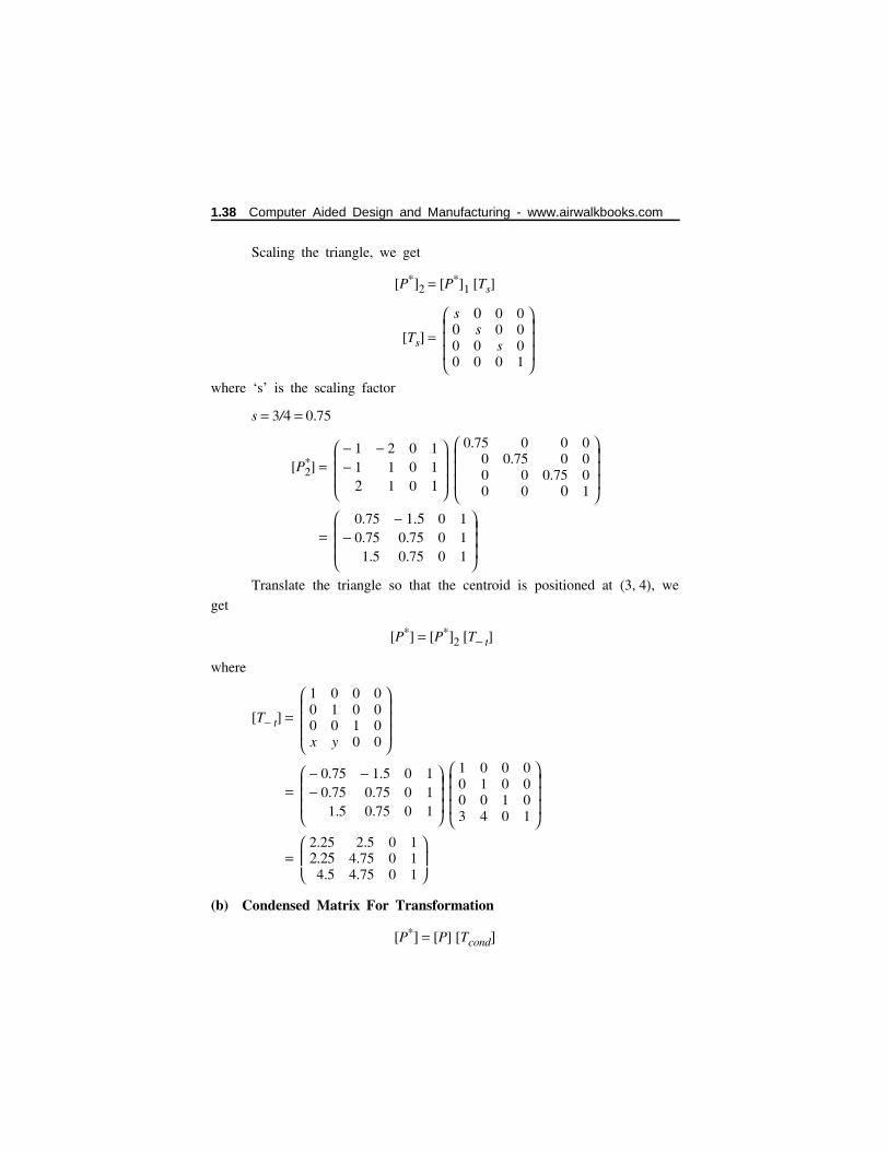
Scaling the triangle, we get

[P∗]2 = [P∗]1 [Ts]

[Ts] =

⎛

⎜

⎝

⎜

⎜

s000

0s00

00s0

0001

⎞

⎟

⎠

⎟

⎟

where ‘s’ is the scaling factor

s = 3/4 = 0.75

[P2∗] =

⎛⎜⎝

⎜⎜ − 1− 1

2

− 211

000

111

⎞⎟⎠

⎟⎟

⎛

⎜

⎝

⎜

⎜

0.75000

00.75

00

00

0.750

0001

⎞

⎟

⎠

⎟

⎟

= ⎛⎜⎝

⎜⎜

0.75− 0.75

1.5

− 1.50.750.75

000

111 ⎞⎟⎠

⎟⎟

Translate the triangle so that the centroid is positioned at (3, 4), weget

[P∗] = [P∗]2 [T− t]

where

[T− t] =

⎛

⎜

⎝

⎜

⎜

100x

010y

0010

0000

⎞

⎟

⎠

⎟

⎟

= ⎛⎜⎝

⎜⎜ − 0.75− 0.75

1.5

− 1.50.750.75

000

111 ⎞⎟⎠

⎟⎟

⎛

⎜

⎝

⎜

⎜

1003

0104

0010

0001

⎞

⎟

⎠

⎟

⎟

= ⎛⎜⎝ 2.252.254.5

2.5

4.754.75

000

111

⎞⎟⎠

(b) Condensed Matrix For Transformation

[P∗] = [P] [Tcond]


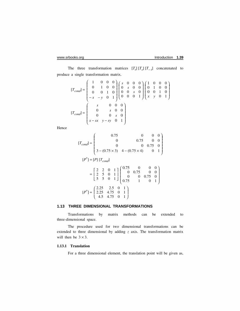
The three transformation matrices [Tt] [Ts] [T− t] concatenated to

produce a single transformation matrix.

[Tcond] =

⎛

⎜

⎝

⎜⎜⎜⎜

100

− x

010

− y

0010

0001

⎞

⎟

⎠

⎟⎟⎟⎟

⎛

⎜

⎝

⎜

⎜

s000

0s00

00s0

0001

⎞

⎟

⎠

⎟

⎟

⎛

⎜

⎝

⎜

⎜

100x

010y

0010

0001

⎞

⎟

⎠

⎟

⎟

[Tcond] =

⎛

⎜

⎝

⎜⎜⎜⎜

s00

x − sx

0s0

y − sy

00s0

0001

⎞

⎟

⎠

⎟⎟⎟⎟

Hence

[Tcond] =

⎛

⎜

⎝

⎜⎜⎜⎜

0.7500

3 − (0.75 × 3)

00.75

04 − (0.75 × 4)

00

0.750

0001

⎞

⎟

⎠

⎟⎟⎟⎟

[P∗] = [P] [Tcond]

= ⎡⎢⎣ 225

255

000

111

⎤⎥⎦

⎛

⎜

⎝

⎜

⎜

0.7500

0.75

00.75

01

00

0.750

0001

⎞

⎟

⎠

⎟

⎟

[P∗] = ⎛⎜⎝ 2.252.254.5

2.5

4.754.75

000

111

⎞⎟⎠

1.13 THREE DIMENSIONAL TRANSFORMATIONS

Transformations by matrix methods can be extended tothree-dimensional space.

The procedure used for two dimensional transformations can beextended to three dimensional by adding z axis. The transformation matrix

will then be 3 × 3.

1.13.1 Translation

For a three dimensional element, the translation point will be given as,


T = (m, n, p) ...(1.7)

where, m, n, p are the coordinates of translation point or increment.

In matrix notation, it is given as,

(x′, y′, z′) = (x, y, z) + T ...(1.8)

1.13.2 Scaling

The scaling transformation is given by,

S = ⎡⎢⎣ m00

0n0

00p ⎤⎥⎦ ...(1.9)

where,

m, n and p are the units needed, to be scaled. For equal values ofm, n and p, the scaling is linear.

1.13.3 Rotation

For each axis, the rotation in three dimensions varies.

For Z axis

Rotation about the Z axis by angle θ is given by the matrix,

Rz = ⎡⎢⎣

⎢⎢ cos θsin θ

0

− sin θcos θ

0

001 ⎤⎥⎦

⎥⎥ ...(1.10)

For Y axis

Rotation about y - axis by angle θ is given by matrix.

Ry = ⎡⎢⎣

⎢⎢

cos θ0

− sin θ

010

sin θ

0cos θ

⎤⎥⎦

⎥⎥ ...(1.11)

For x axis

Rotation about x - axis by angle θ is given by matrix,

Rx = ⎡⎢⎣

⎢⎢ 100

0

cos θsin θ

0

− sin θcos θ

⎤⎥⎦

⎥⎥ ...(1.12)


1.14 HOMOGENEOUS COORDINATES REPRESENTATION

What is homogeneous coordinate? (AU. Nov/Dec 2016)

The difficulty in image manipulation, incorporating all the five typesof geometric transformations, can be removed if represented by a single matrixequation. This will be possible only if points are represented in homogeneouscoordinates.

The homogeneous coordinates are obtained by adding the thirdcoordinate to a point.

This facilitates the image manipulation with a single transformationmatrix for all types of geometric transformations.

In homogeneous coordinate system, mapping between the

n-dimensional spaces with (n + 1) dimensional spaces occur, it points inn-dimensional coordinates are represented by the corresponding

(n + 1)-dimensional coordinates.

This is obtained by introducing a scale factor along the cartesiancoordinates.

For 2D coordinates, instead of being represented by a pair (x, y), each

point is represented by triple coordinates (x′, y′, h) where h ≠ 0, is the scalarfactor.

The relationship between the cartesian coordinates and homogeneouscoordinates of a point is given by,

x = x′h

; y = y′h

(i.e)

x′ = xh; y′ = yh ...(1.13)

Generally, h = 1 represents a homogeneous coordinate (x, y, 1) for a

point (x, y) in computer graphics.

Two sets of homogeneous coordinates (x, y, h) and (x′, y′, h′) representthe same point if and only if one is a multiple of the other.


Different homogeneous coordinates can represent each point. Forexample: homogeneous coordinates of a point (3,2) may be expressed by thecoordinate triple as (3,2,1) or (6,4,2) or (9,6,3). If we take all triplesrepresenting the same point, we get a line in 3D space.

Each homogeneous point represents a line in 3D space. If these points

are homogenized points from the plane, defined by equation h = 1, in

(x, y, h) space is shown in Fig. 1.13. Graphically, the scale factor h may beinterpreted as the cartesian image on a plane parallel to the xy plane and atunit distance away from the origin along z - direction.

The points with h = 0 are called points at infinity (not represented onthe planes), and will not appear very often in the discussion.

This type of visualization is not possible in 3D geometrictransformations.

In computer graphics, we shift the coordinates of the object model

from (x, y) coordinate space to (x, y, 1) coordinate space, keeping h = 1. Thus‘1’ should be added while defining any coordinate in 2D.

For example, a point in 3D − (3, 4, 2) should be represented as (3, 4,2, 1).

yy′

x

x′

h

h=1

Fig:1.13 .The (x ,y,h) Hom ogeneous Coordinate Space W ith h=1 Plane

Th ird P r incipa l A xis P erpendicu la r to xy P lane


1.15 HOMOGENEOUS TRANSFORMATION MATRICES

In generalized form, the matrix equation incorporating all five typesof geometric transformations may be expressed as

⎧

⎨

⎩

⎪

⎪

xTyT1

⎫

⎬

⎭

⎪

⎪ =

⎡⎢⎣ AC0

BD0

001 ⎤⎥⎦ ⎧

⎨

⎩

⎪

⎪ xy1

⎫

⎬

⎭

⎪

⎪ = [T]

⎧

⎨

⎩

⎪

⎪ xy1 ⎫

⎬

⎭

⎪

⎪...(1.14)

where,

[T] → Transformation matrix in homogeneous coordinates.

1.15.1 Translation

The translation of homogeneous matrix is given as,

[Tt] = ⎡⎢⎣

⎢⎢

100

010

txty1 ⎤⎥⎦

⎥⎥ ...(1.15)

1.15.2 Scaling

The scaling of homogeneous matrix is given by

[S] = ⎡

⎢

⎣

⎢

⎢

Sx00

0Sy0

001

⎤

⎥

⎦

⎥

⎥ ...(1.16)

1.15.3 Rotation

For homogeneous transformation, counter clockwise rotation (CW) inthe xy plane is given by,

[Tr] = ⎡⎢⎣

⎢⎢ cos αsin α

0

− sin αcos α

0

001 ⎤⎥⎦

⎥⎥ ...(1.17)

For homogeneous transformation, clockwise rotation (CW) in xy planeis given by,

[Tr] = ⎡⎢⎣

⎢⎢

cos α− sin α

0

− sin αcos α

0

001 ⎤⎥⎦

⎥⎥ ...(1.18)


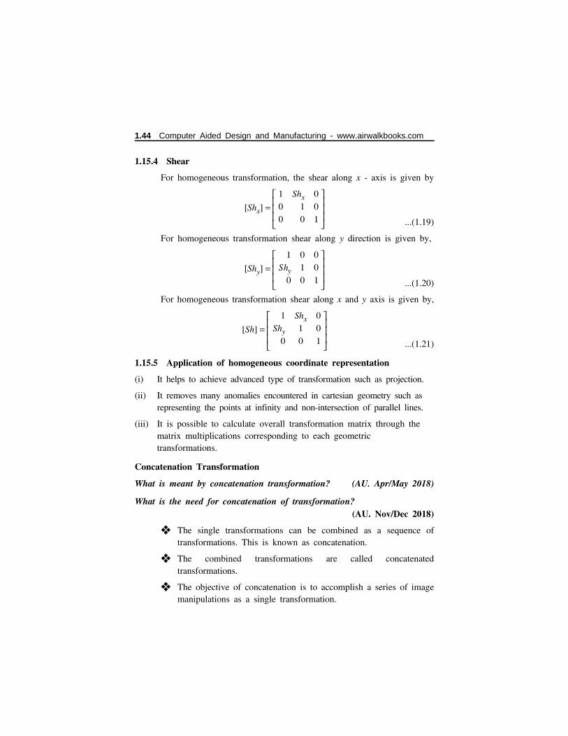
1.15.4 Shear

For homogeneous transformation, the shear along x - axis is given by

[Shx] = ⎡

⎢

⎣

⎢

⎢

100

Shx10

001 ⎤

⎥

⎦

⎥

⎥ ...(1.19)

For homogeneous transformation shear along y direction is given by,

[Shy] = ⎡

⎢

⎣

⎢

⎢

1Shy

0

010

001 ⎤

⎥

⎦

⎥

⎥ ...(1.20)

For homogeneous transformation shear along x and y axis is given by,

[Sh] = ⎡

⎢

⎣

⎢

⎢

1Shy

0

Shx10

001

⎤

⎥

⎦

⎥

⎥ ...(1.21)

1.15.5 Application of homogeneous coordinate representation

(i) It helps to achieve advanced type of transformation such as projection.

(ii) It removes many anomalies encountered in cartesian geometry such asrepresenting the points at infinity and non-intersection of parallel lines.

(iii) It is possible to calculate overall transformation matrix through thematrix multiplications corresponding to each geometrictransformations.

Concatenation Transformation

What is meant by concatenation transformation? (AU. Apr/May 2018)

What is the need for concatenation of transformation?(AU. Nov/Dec 2018)

❖ The single transformations can be combined as a sequence oftransformations. This is known as concatenation.

❖ The combined transformations are called concatenatedtransformations.

❖ The objective of concatenation is to accomplish a series of imagemanipulations as a single transformation.


❖ This allows the concatenated transformation to be defined moreconcisely and the computation can generally be accomplishedefficiently.

1.16 LINE DRAWING

Explain a line drawing algorithm. (AU. Nov/Dec 2016)

Line can be created by calculating the intermediate position along theline path between two end points.

In a vector display, a line can be drawn smoothly from one end pointto the other. Depending on the changes in x and y directions, different linescan be drawn.

A line drawing algorithm must satisfy the following features:

❖ On the display device, line should appear straight.

❖ Line should terminate accurately at the end.

❖ Constant density of the line should be maintained through out the length.

❖ Line should be drawn accurately.

By joining up the two end points by discrete points a line can bedrawn. The coordinate positions of the discrete points along the line path arecalculated from the equation of the line.

Two important methods of generating a line segment are given below:

1. Digital Differential Analyser - (DDA) Algorithm

2. Bresenham’s line Algorithm

1.16.1 Digital differential analyzer algorithm

Describe and demonstrate DDA line drawing algorithm.(AU. Apr/May 2018)

Digital differential analyzer is a scan conversion line-generating

algorithm, based on the calculation of either Δ y or Δ x differences along theline path.

A line can be generated by increasing unit interval in one coordinateand determining the corresponding integer values of interval in othercoordinate nearest to the line path.


The equation of straight line is given as,

y = mx + b ...(1.22)

where,

m → slope

m = y2 − y1

x2 − x1 ...(1.23)

= Δ y

Δ x

For any value of Δ x, we can compute the corresponding Δ y by theequation.

Δ y = m Δ x ...(1.24)

Similarly for any value of Δ y, we can compute the corresponding

Δ x by the equation.

Δ x = Δ ym ...(1.25)

There are two possibilities of slope, either m < 1 or m > 1.

Slope Less Than 1 (i.e ) m <1 Slope More Than 1 (i.e) m>1Fig:1.14 Lines in Raster Device with Positive Slope.


Fig. 1.14 shows the two lines with positive slope on the raster scandisplays.

Case (i)

If slope is less than 1 (i.e) m < 1 is positive

Consider the increment in x coordinate as unity, and the line starts

from left and extends (i.e) Δ x = 1.

If (xk, yk) is any current point on the line path, then next point will be

xk + 1 = xk + 1 and yk + 1 = yk + m because for Δ x = 1, Δ y = m Δ x = m.1 = m.

Similarly if line starts from right, the procedure remains same except

that the new coordinate will be xk + 1 = xk − 1 and yk + 1 = yk − m.

Case (ii)

If slope is greater than 1 (i.e) m > 1 and it is positive

Let the line starts from left and extends to the right with unit increment

in y coordinate, i.e., Δ y = 1.

If (xk, yk) is any current point on the line path, then the next point

will be yk + 1 = yk + 1 and xk + 1 = xk + 1m

, because for Δ y = 1, Δ x = Δ ym

= 1m

.

Similarly if line starts from right, the procedure remains same except

that the new coordinate will be yk + 1 = yk − 1 and xk + 1 = xk − 1m

Case (iii)

If m < 1 and slope is negative

Consider the line starts from right, the procedure given for m < 1. (case

i), follows with modification that as one coordinate (x) decreases, other

coordinate (y) increases ∴ New coordinate will be,

xk + 1 = xk − 1 and yk + 1 = yk + m


Case (iv)

If m > 1 and slope is negative

Consider the line starts from right to left, the procedure given for

m > 1 (case (ii)) follows with the modification that as one coordinate (y)decreases, other coordinate (x) increases.

∴ New coordinate will be

yk + 1 = yk − 1 and xk + 1 = xk + 1m

Digital differential analyzer algorithm generates a straight line at a fastspeed.

Problem 1.8: Draw a straight line connecting two end points (2,7) and(15,10).

Given data

x1 = 2; x2 = 15

y1 = 7; y2 = 10

To find

Draw a straight line from given points.

Solution

x2 − x1 = 15 − 2

= 13

y2 − y1 = 10 − 7

= 3

m = slope = y2 − y1

x2 − x1

= 3

13

= 0.23076


Since slope m < 1 and positive. This comes under case (i) therefore,new coordinates will be

xk + 1 = xk + 1

yk + 1 = yk + m

The intermediate pixels from point A to B are calculated. The tableshows the intermediate pixel positions and line is shown Fig.

KInteger valuesxk + 1 = xk + 1

Real valuesyk + 1 = yk + m

(Round of)Integer valuesyk + 1 = yk + m

0 2 – 7

1 3 7.230 7

2 4 7.46 7

3 5 7.69 8

4 6 7.92 8

5 7 8.15 8

6 8 8.38 8

7 9 8.61 9

8 10 8.84 9

9 11 9.07 9

10 12 9.3 9

11 13 9.53 10

12 14 9.76 10

13 15 9.99 10 (accurate)


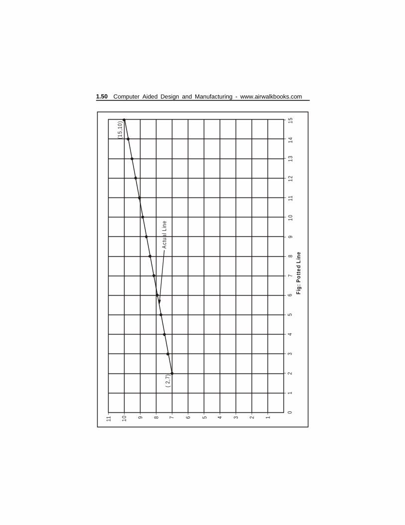
1234567891011

01

23

45

67

89

1011

1213

1415

( 2,

7)

(15,

10)

Act

ual L

ine

Fig

: P

ott

ed L

ine


Problem 1.9: Digitize the line with end points A (20,10) and B (10,18)using DDA algorithm.

Given data

x1 = 20; x2 = 10

y1 = 10; y2 = 18

To find:

Obtaining the line with DDA algorithm

Solution

x2 − x1 = 10 − 20 = − 10

y2 − y1 = 18 − 10 = 8

slope, m = Δ yΔ x

= y2 − y1

x2 − x1

= 8

− 10 = − 0.80

since slope m < 1 and negative

It is case (iii)

Therefore, new coordinates will be,

xk + 1 = xk − 1

yk + 1 = yk + m

= yk + 0.80

The intermediate points between A and B are calculated as given inTable.


KInteger valuexk + 1 = xk − 1

Real valueyk + 1 = yk + m

Integer valueyk + 1 = yk + m

0 20 – 10

1 19 10.80 11

2 18 11.60 12

3 17 12.40 12

4 16 13.20 13

5 15 14.00 14

6 14 14,80 15

7 13 15.60 16

8 12 16.40 16

9 11 17.20 17

10 10 18.00 18

10

12

14

16

18

20

24

22

(10,18 )

Ac tu al line

(20,10 )

10 12 14 16 18 20 2422Fig. Plotted line


1.16.2 Bresenham’s line drawing algorithm

Bresenham’s line drawing algorithm rectifies the disadvantage of digitaldifferential analyzer algorithm.

Bresenham’s developed an accurate and efficient method of rastergeneration algorithms to display lines, circles, ellipse and other curvesincorporating only incremental integer calculation.

The features of Bresenham’s line drawing algorithm are given below:

(i) The line generated by Bresenham’s technique uses standard equation

of line (y = mx + c).

❖ A non-negative integer (x, y) coordinate pair access each pixel.

❖ Line always starts from left irrespective of the input from the user.Bresenham’s algorithm decides the one which is lying on the leftas starting point.

1.16.3 Procedure for line generation when slope m < 1

i.e. slope is between 0° and 45°Step: 1

Input the line end points AB as (x1, y1) and (x2, y2) respectively.

Step: 2

Plot the first end point (x1, y1) which means load the point into the

frame buffer.

Step: 3Calculate the initial value of decision parameters, Pk i.e. Po

Δ x = x2 − x1

Δ y = y2 − y1

Po = 2Δ y − Δ x

Step: 4

At each xk position, starting from K = 0, perform the following test:

If P < 1 (negative), the next position for plotting the pixel is

(xk + 1, yk) and Pk + 1 = Pk + 2Δ y.


If P > 1 (positive) the next pixel position is (xk + 1, yk + 1) and

Pk + 1 = Pk + 2Δ y − 2Δ x

Step: 5

Plot the point of current (x, y) position.

Step: 6

Repeat step 4 through step 5, Δ x times until the second end point is

reduced i.e. x ≥ x2.

1.16.4 Procedure for generating the line when slope m > 1

(i.e) slope is between 45° and 90°The procedure is same except that x and y coordinates are interchanged.

Step: 1

Input the line end points AB as (x1, y1) and (x2, y2) respectively.

Step: 2

Plot the first end point (x1, y1) which means load the point into the

frame buffer.

Step: 3Calculate the initial value of the decision parameter Pk (i.e) Po.

Δ x = x2 − x1

Δ y = y2 − y1

Po = 2Δ x − Δ y

Step: 4

At each xk position, from K = 0, perform the following test:

If Pk < 1 (negative) the next position to plot the pixel is (xk, yk + 1)

and Pk + 1 = Pk + 2Δ x

If Pk > 1 (positive) the next pixel position is, (xk + 1, yk + 1) and

Pk + 1 = Pk + 2Δ x − 2Δ y


Step: 5

Plot the point of current (x, y) position

Step: 6

Repeat step 4 through step 5, Δ y times until reaching the second end

point. i.e, y ≥ y2.

Problem 1.10: Draw the line using Bresenham’s algorithm with the endpoints A (18,8) and B (28,16).

Given data

x1 = 18; y1 = 8

x2 = 28; y2 = 16

To findObtain the line using Bresenham’s algorithm.

Solution

Δ x = x2 − x1 = 28 − 18 = 10

Δ y = y2 − y1 = 16 − 8 = 8

Slope, m = Δ y

Δ x =

810

= 0.80

Since slope m < 1 and positive

Then,

Po = 2Δ y − Δ x

successive values of the decision parameter,

Pk + 1 = Pk + 2Δ y − 2Δ x ⋅ (yk + 1 − yk)

If Pk < 1, the next pixel position to plot is (xk + 1, yk) and

Pk + 1 = Pk + 2Δ y

Otherwise Pk > 1, the next pixel position is (xk + 1, yk + 1) and

Pk + 1 = Pk + 2Δ y − 2Δ x


KDecision parameter

Pk

Value of decisionparameter

Pk

Next pixelValue

of nextpixel

0 P0 = 2Δ y − Δ x 2 (8) − 10 = 6 (xk + 1, yk + 1)

1 P1 = P0 + 2Δ y − 2Δ x 6 + 2 (8) − 2 (10) = 2 (xk + 1, yk + 1) (20,10)

2 P2 = P1 + 2Δ y − 2Δ x 2 + 2 (8) − 2 (10) = − 2 (xk + 1, yk) (21,10)

3 P3 = P2 + 2Δ y − 2 + 2 (8) = 14 (xk + 1, yk + 1)

4 P4 = P3 + 2Δ y − 2Δ x 14 + 2 (8) − 2 (10) = 10 (xk + 1, yk + 1) (23,12)

5 P5 = P4 + 2Δ y − 2Δ x 10 + 2 (8) − 2 (10) = 6 (xk + 1, yk + 1) (24,13)

6 P6 = P5 + 2Δ y − 2Δ x 6 + 2 (8) − 2 (10) = 2 (xk + 1, yk + 1) (25,14)

7 P7 = P6 + 2Δ y − 2Δ x 2 + 2 (8) − 2 (10) = − 2 (xk + 1, yk) (26,14)

8 P8 = P7 + 2Δ y − 2 + 2 (8) = 14 (xk + 1, yk + 1) (27,15)

9 P9 = P8 + 2Δ y − 2Δ x 14 + 2.8 − 2 (10) = 10 (xk + 1, yk + 1) (28,16)

8

10

12

14

16

18

22

20

16 18 20 22 24 26 30

Actual L ine

(2 8,16 )

28

B

A (1 8,8 )

P ixe l N ox

Pix

el N

oy


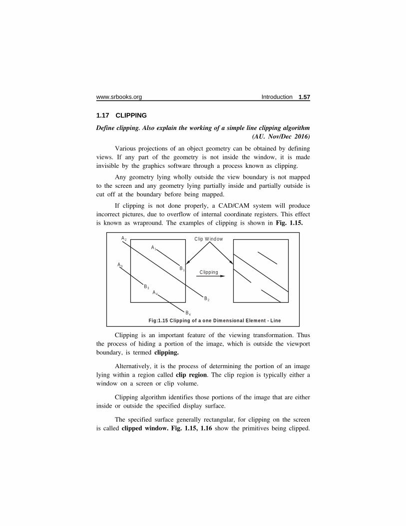
1.17 CLIPPING

Define clipping. Also explain the working of a simple line clipping algorithm(AU. Nov/Dec 2016)

Various projections of an object geometry can be obtained by definingviews. If any part of the geometry is not inside the window, it is madeinvisible by the graphics software through a process known as clipping.

Any geometry lying wholly outside the view boundary is not mappedto the screen and any geometry lying partially inside and partially outside iscut off at the boundary before being mapped.

If clipping is not done properly, a CAD/CAM system will produceincorrect pictures, due to overflow of internal coordinate registers. This effectis known as wrapround. The examples of clipping is shown in Fig. 1.15.

Clipping is an important feature of the viewing transformation. Thusthe process of hiding a portion of the image, which is outside the viewportboundary, is termed clipping.

Alternatively, it is the process of determining the portion of an imagelying within a region called clip region. The clip region is typically either awindow on a screen or clip volume.

Clipping algorithm identifies those portions of the image that are eitherinside or outside the specified display surface.

The specified surface generally rectangular, for clipping on the screenis called clipped window. Fig. 1.15, 1.16 show the primitives being clipped.

A 1

A 2

A 3

A 4

B 3

B 1

B 4

B 2

C lipp ing

C lip W ind ow

Fig:1.15 Clipping of a one Dim ensional Element - Line


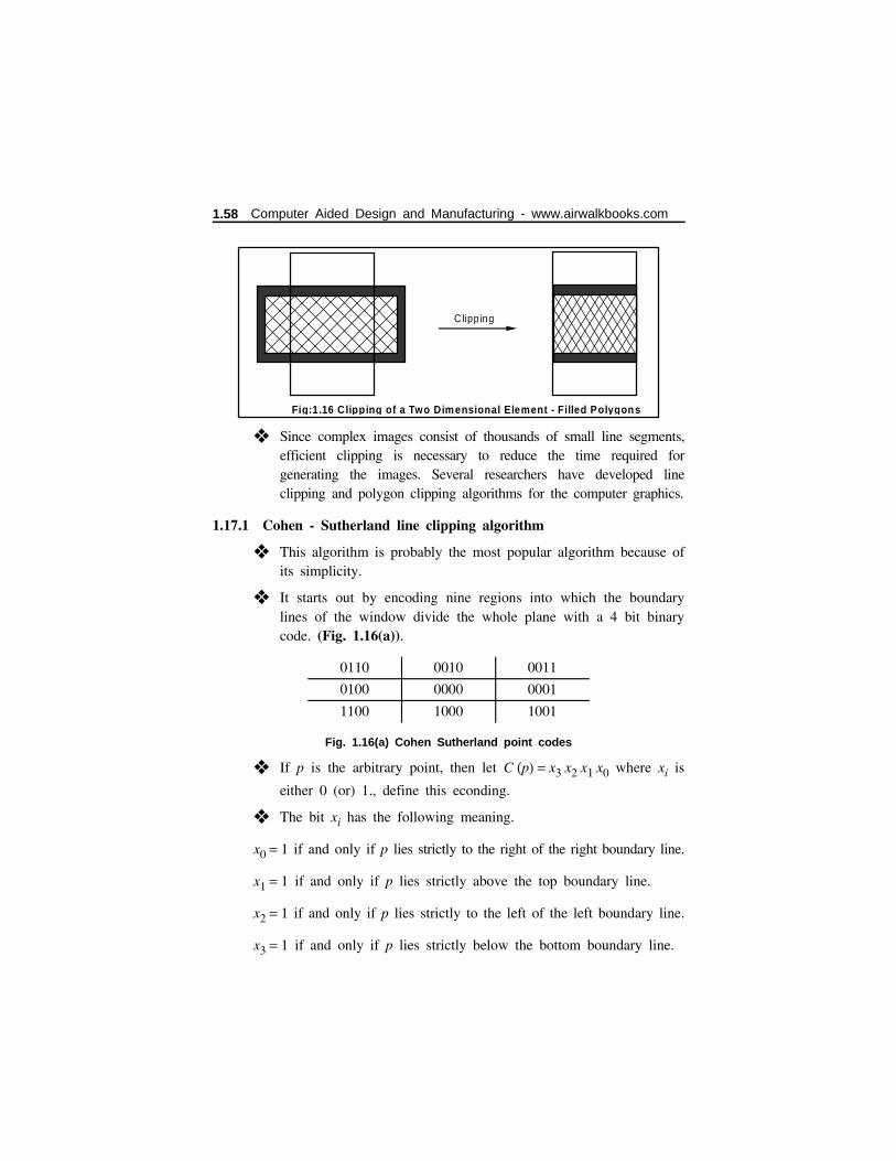
❖ Since complex images consist of thousands of small line segments,efficient clipping is necessary to reduce the time required forgenerating the images. Several researchers have developed lineclipping and polygon clipping algorithms for the computer graphics.

1.17.1 Cohen - Sutherland line clipping algorithm

❖ This algorithm is probably the most popular algorithm because ofits simplicity.

❖ It starts out by encoding nine regions into which the boundarylines of the window divide the whole plane with a 4 bit binarycode. (Fig. 1.16(a)).

0110 0010 0011

0100 0000 0001

1100 1000 1001

Fig. 1.16(a) Cohen Sutherland point codes

❖ If p is the arbitrary point, then let C (p) = x3 x2 x1 x0 where xi is

either 0 (or) 1., define this econding.

❖ The bit xi has the following meaning.

x0 = 1 if and only if p lies strictly to the right of the right boundary line.

x1 = 1 if and only if p lies strictly above the top boundary line.

x2 = 1 if and only if p lies strictly to the left of the left boundary line.

x3 = 1 if and only if p lies strictly below the bottom boundary line.

Clipp ing

Fig:1.16 Clipping of a Two Dimensional Element - Filled Polygons


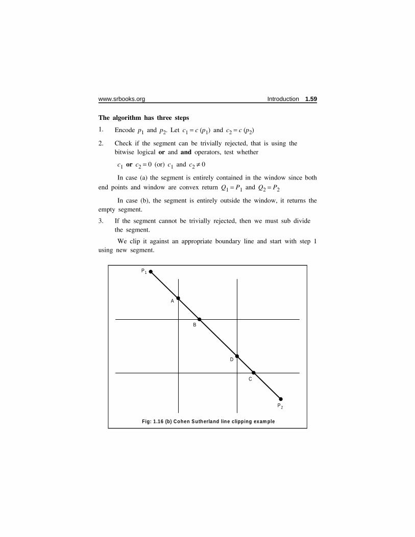
The algorithm has three steps

1. Encode p1 and p2. Let c1 = c (p1) and c2 = c (p2)

2. Check if the segment can be trivially rejected, that is using thebitwise logical or and and operators, test whether

c1 or c2 = 0 (or) c1 and c2 ≠ 0

In case (a) the segment is entirely contained in the window since both

end points and window are convex return Q1 = P1 and Q2 = P2

In case (b), the segment is entirely outside the window, it returns theempty segment.

3. If the segment cannot be trivially rejected, then we must sub dividethe segment.

We clip it against an appropriate boundary line and start with step 1using new segment.

A

B

D

C

P2

P1

Fig: 1.16 (b) Cohen Sutherland line clipping exam ple


❖ In this case, we have to clip four times.

❖ It is to be clipped successively against each one of the windowboundary lines generating the intersection points A, B, C and D.

1.18 VIEWING TRANSFORMATION

Deduce windowing and viewing transformation matrices parametrically.(AU. Nov/Dec 2016)

What is meant by view port and windowing? (AU. Nov/Dec 2017)

The complex drawings of an object or element in world coordinatesystem has become very difficult to visualize. In such cases a window isrequired to visualize portions of the drawing on the display surface.

The selected area in the world space, with the sides parallel to x andy directions of the world coordinate system, is called a window, and methodof selecting and enlarging portions of drawing on the display is termedwindowing.

On the display surface the image lies within the window.

Thus viewing transformation is capable of displaying generated imagesthe way the user wants to present. This function set provides the user withthe ability to view the image from the desired angle and at the desiredmagnification.

In windowing transformation, the graphics screen behaves as a windowfor display of the application model. In windowing process we may not usethe entire screen for display, but we see the area within a box. Such box iscalled as viewport.

Fig. 1.17 shows different stages of the viewing transformation fromwindows to viewport.

W ind ow No rm alized V ie w Port V iew Port

Im age inW orld Coord inate

System

M apping to No rm alized

Co ord inate S ys tem

M apping ToDe vice C oord in a te

System

Fig:1 .17 Viewing Transform ation of Im age


In fact, viewing transformation is the process of mappingcoordinates/points from window onto the viewport.

Viewing transformation is the operation of a transformation matrix onthe coordinates of every point of the object.

Fig. 1.18 shows the windowing operation to display certain areas ofthe image on different viewports.

W orld Coord inates x

y

Fig:1.18. (a) Different Windows on Different Viewports

Fig:1.18. (b) Sam e Window on Different Viewports

W indow - I

W indow - II

View PortII

View PortI

Device Coordinates

W orld Coord inates x

y

W indow

View PortII

View PortI

Device Coordinates


1.19 BRIEF INTRODUCTION TO CAD AND CAM

CAD means Computer Aided Design and CAM means

Computer Aided Manufacturing.

CAD is defined as the use of computer systems to assist in the creation,modification, Analysis (or) optimization of a design.

CAM can be defined as the use of computer systems to plan, manage& control the operations of a manufacturing plant through either direct (or)indirect computer interface with production resources.

Computer system consists of the hardware and software to perform thespecialized design functions required by the particular user firm.

1.20 COMPUTER AIDED DESIGN (CAD)

1.20.1 What is CAD?

It is the technology used to integrate the design activities with the helpof computer which includes transformation and modification of images of partgeometry, printing the images on a printer or plotter and design data analysis.

CAD can als o b e defined a s the proces s in which computers areutilised in the creation of model, modification and analysis of a design to getthe optimum model.

1.20.2 Why should we go for CAD?

1. For improved documentation, more standardization, betterEngineering drawings, reduced drawing errors and clear perceptionof drawings.

2. The design quality is improved, moreover any problem encounteredduring design can be rectified and suitable alternatives are suggested.There is an inbuilt feature which checks for any calculation errorsand leads to better quality and accuracy of design.

3. The productivity is increased, the synthesis time is greatly reducedas the design engineer has better visualisation of part geometry.


1.20.3 The factors to be considered while selecting a CAD system

(a) Reliability

(b) Compatibility with other system

(c) Cost Factors

(d) Memory size and storage requirement

(e) Type of peripherals requirement.1.2.4. Role of Computer in CAD:

1.20.4 Role of Computer in CAD

(a) Computer improves accuracy of design.

(b) Various dimension and other design attributes can be convenientlymanipulated by computers.

(c) A nother im port ant rol e pla y ed by Computers is creation ofpart libraries for standard components. Similarly multiple componentscan be included in these part libraries.

(d) Moreover, the modification of a model is very simple which he lpsthe des ig ner to look i n for further improvement.

(e) Calculation of various geometric properties such as area, volume anddimensioning can be accurately done.

1.20.5 Applications of CAD in simple words

(a) Finite element analysis.

(b) CNC programming.

(c) Building drawing using Architectural CAD.

(d) Piping system for Engineering Industries.

(e) CAPP (Computer Aided Process Planning).

(f) Kinematic analysis for systems.

(g) Dynamic analysis for systems.

1.20.6 Uses of CAD

(a) Creating several colour combinations for a product to improve itsappeal.

(b) Exploded views of assemblies can be effectively done.


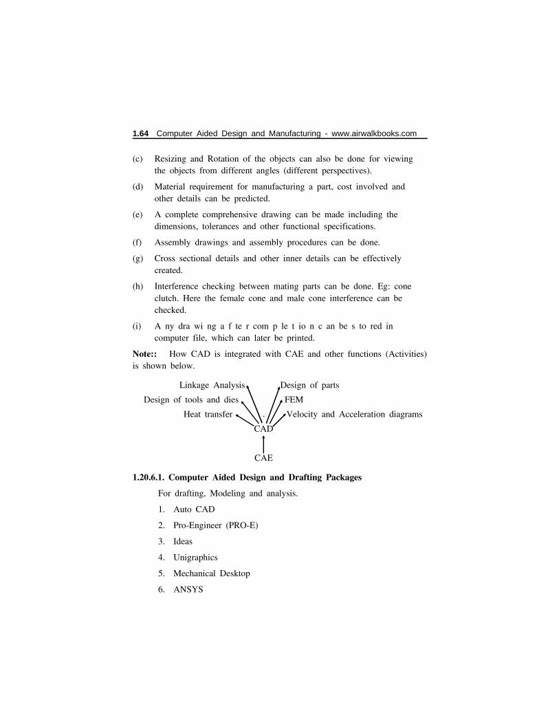
(c) Resizing and Rotation of the objects can also be done for viewingthe objects from different angles (different perspectives).

(d) Material requirement for manufacturing a part, cost involved andother details can be predicted.

(e) A complete comprehensive drawing can be made including thedimensions, tolerances and other functional specifications.

(f) Assembly drawings and assembly procedures can be done.

(g) Cross sectional details and other inner details can be effectivelycreated.

(h) Interference checking between mating parts can be done. Eg: coneclutch. Here the female cone and male cone interference can bechecked.

(i) A ny dra wi ng a f te r com p le t io n c an be s to red incomputer file, which can later be printed.

Note:: How CAD is integrated with CAE and other functions (Activities)is shown below.

Linkage Analysis Design of parts

Design of tools and dies FEM

Heat transfer Velocity and Acceleration diagrams

CAD

CAE

1.20.6.1. Computer Aided Design and Drafting Packages

For drafting, Modeling and analysis.

1. Auto CAD

2. Pro-Engineer (PRO-E)

3. Ideas

4. Unigraphics

5. Mechanical Desktop

6. ANSYS


7. Nastran

8. Pro-Mechanica

9. CATIA

1.20.7 Reasons for Implementing a CAD

❖ To create and modify appearance of objects.

❖ It improves the productivity of the designer.

❖ Improves communication.

❖ Improves the efficiency of Design.

❖ Create database for manufacturing.

1.20.8 Benefits of CAD

1. Increased design and productivity.

2. Flexibility in design.

3. Improved design analysis.

4. Greater accuracy in design.

5. Easier creation and correction of engineering drawings.

6. Better visualization of drawings.

7. Faster new product design.

8. Shorter lead time.

1.20.9 Applications of CAD

Table 1.2

Area Applications

Design Assembly layout,

New-part design,

Standard part library,

Tolerance specifications,

Clearance specifications


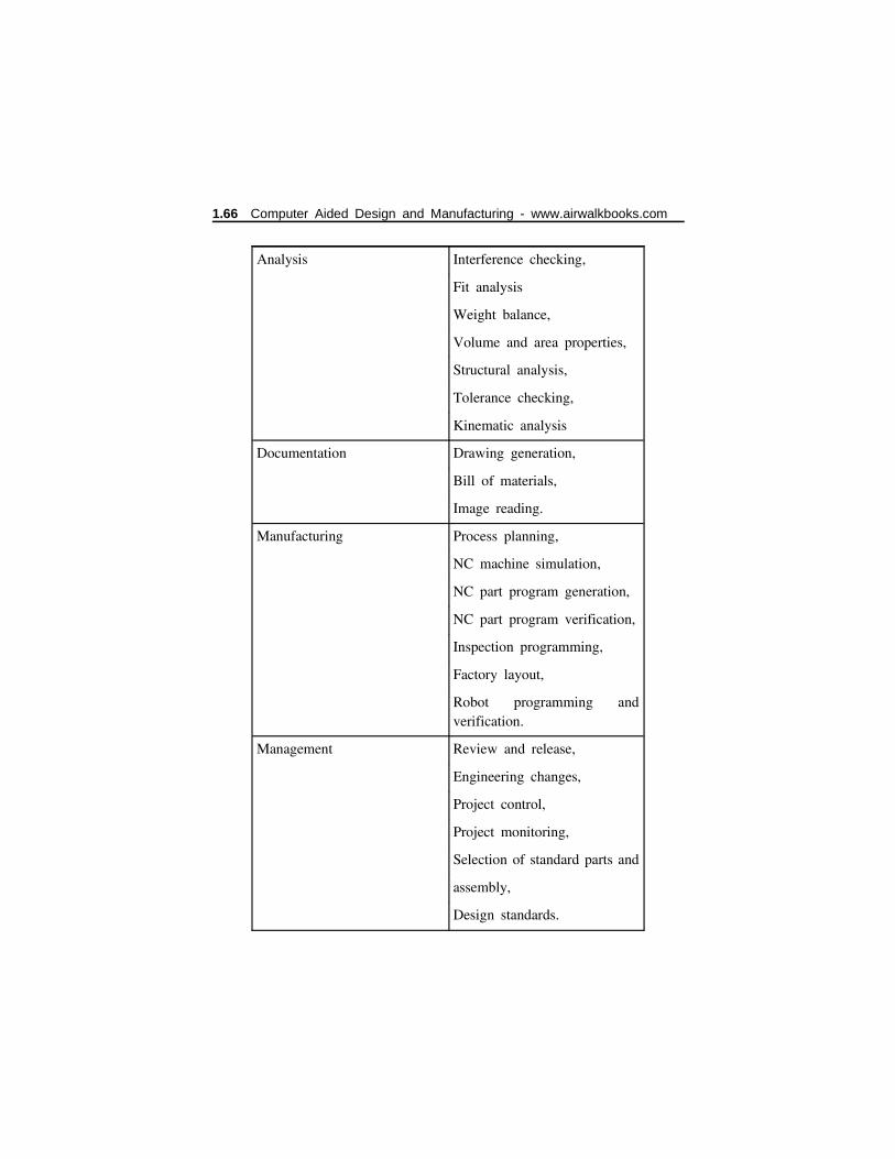
Analysis Interference checking,

Fit analysis

Weight balance,

Volume and area properties,

Structural analysis,

Tolerance checking,

Kinematic analysis

Documentation Drawing generation,

Bill of materials,

Image reading.

Manufacturing Process planning,

NC machine simulation,

NC part program generation,

NC part program verification,

Inspection programming,

Factory layout,

Robot programming andverification.

Management Review and release,

Engineering changes,

Project control,

Project monitoring,

Selection of standard parts and

assembly,

Design standards.


1.21 DESIGN PROCESS IN CAD SYSTEM (OR) ELEMENTS OF A CAD

Explain with block diagram, the CAD process with suitable examples.(AU. Apr/May 2017)

The various design related tasks which are performed by a moderncomputer aided design system can be grouped into four functional areas:

1. Geometric modeling

2. Engineering analysis

3. Design review and evaluation

4. Automated drafting

R e cogn it io n o f n eed

Problemdefin ition

Synthe s is

An alys is andoptim ization

Evalua tion

Presen tation

G eom etricm od eling

D e sign reviewand eva luation

Au to m ated dra ft ing

The design process Com puter-aided design

En gine er ingAn alys is


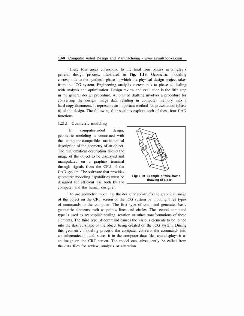
These four areas correspond to the final four phases in Shigley’sgeneral design process, illustrated in Fig. 1.19. Geometric modelingcorresponds to the synthesis phase in which the physical design project takesfrom the ICG system. Engineering analysis corresponds to phase 4, dealingwith analysis and optimization. Design review and evaluation is the fifth stepin the general design procedure. Automated drafting involves a procedure forconverting the design image data residing in computer memory into ahard-copy document. It represents an important method for presentation (phase6) of the design. The following four sections explore each of these four CADfunctions.

1.21.1 Geometric modeling

In computer-aided design,geometric modeling is concerned withthe computer-compatible mathematicaldescription of the geometry of an object.The mathematical description allows theimage of the object to be displayed andmanipulated on a graphics terminalthrough signals from the CPU of theCAD system. The software that providesgeometric modeling capabilities must bedesigned for efficient use both by thecomputer and the human designer.

To use geometric modeling, the designer constructs the graphical imageof the object on the CRT screen of the ICG system by inputing three typesof commands to the computer. The first type of command generates basicgeometric elements such as points, lines and circles. The second commandtype is used to accomplish scaling, rotation or other transformations of theseelements. The third type of command causes the various elements to be joinedinto the desired shape of the object being created on the ICG system. Duringthis geometric modeling process, the computer converts the commands intoa mathematical model, stores it in the computer data files and displays it asan image on the CRT screen. The model can subsequently be called fromthe data files for review, analysis or alteration.

Fig: 1.20 Example of wire-framedrawing of a part


There are several different methods of representing the object ingeometric modeling. The basic form uses wire frames to represent the object.In this form, the object is displayed by interconnecting lines, as shown inFig. 1.20. Wire-frame geometric modeling is classified into three types,depending on the capabilities of the ICG system. The three types are:

1. 2D. Two-dimensional representation is used for a flat object.

2. 2 1/2 D. This goes somewhat beyond the 2D capability bypermitting a three-dimensional object to be represented as long as ithas no side-wall details.

3. 3D. This allows for full three-dimensional modeling of a morecomplex geometry.

1.21.2 Engineering Analysis

❖ In the formulation of nearly any Engineering design project, sometypes of analysis is required.

❖ The analysis may involve stress-strain calculations, heat transfer oruse of differential equations to describe the dynamic behaviour ofthe system being designed.

❖ CAD/CAM systems often include engineering analysis softwarewhich can be called to operate on the current design model.

Example:

1. Analysis of mass properties

2. Finite element analysis

3. Design, Review & evaluation

❖ Checking the accuracy of the design can be accomplishedconveniently on the graphics terminal.

❖ A procedure called layering is often helpful in design review.Eg: A good application of layering involves overlaying thegeometric image of the final. Shape of the machined part on thetop of the image in the rough casting.

❖ Another procedure for design review is interference checking.


4. Automated drafting

❖ It involves the creation of hardcopy engineering drawings directlyfrom the CAD database.

❖ CAD systems can increase productivity in the drafting functionmore over 5 times of manual drafting.

❖ This feature includes automatic drawing, hatched areas, scaling,zoom, etc.

1.22 COMPUTER AIDED MANUFACTURING (CAM)

The computer systems are used to plan, mangage and control theoperations of the production plant through the computer interface with theplant’s production resources. This is known as Computer AidedManufacturing. CAM is most closely assoicated with process planning andnumerical control (NC) part programming.

The functions of CAM are given below.

1. Computer Aided Process Planning (CAPP)

2. CNC Part Programming

3. Computer Aided Work Standards

4. Production Scheduling

5. Materials Requirements Planning (MRP)

6. Shop Floor Control

The advantages of Computer Aided Manufacturing

The Computer application in manufacturing makes use of commondatabase. The data is transferred from one function to another automaticallyto give a base for the concept of Computer Integrated Manufacturing (CIM).

The other advantages of CAM are given below:

1. Increased Productivity.

2. Shorter lead time

3. Improved reliability.

4. Freedom in modifying design.


5. Flexibility in operations.

6. Reduced scrap and rework.

7. Reduced Maintenance.

8. Better Control of Management.

The application of CAM can be classified into two categories:

1. Manufacturing planning

2. Manufacturing control

1.22.1 Manufacturing planning

In this process computer is used indirectly to support the productionfunction, but there is no direct connection between the computer and process.

Production System

Facilities

ProductionDesign

M anufactu ring Planning

Business Functions

M anufactu ring Control

Custom erOrder

Fig:1.21 The Information- processing Cycle in a Typical Manufacturing Firm


Important Applications are:

1. CAPP - Computer Aided Process Planning

2. Computer Assisted NC part programming

3. Computerized machinability data systems

4. Computerized work standards

5. Cost Estimating

6. Production and Inventory planning

7. Computer Aided line balancing

1.22.2 Manufacturing control

Manufacturing control is concerned with managing and controlling thephysical operations in the factory.

The following areas to be controlled by manufacturing control,

1. Process monitoring

2. Quality control

3. Shop floor control

4. Inventory control

5. First in time production.

1.22.3 CAD/CAM Interface

CAD/CAM is concerned with the engineering functions in both designand manufacturing.

CAD/CAM must be interfaced to achieve improvement inmanufacturing, improved productivity and quality. The various data (likecomponent geometry data) generated for designing and developing CADdrawings can be reused for manufacturing instruction. These data can be usedfor CNC production processes. Computer Aided Process Planning (CAPP),Computer aided production planning and control (PPC) and shop floor control(SFC). The CNC production processes CAPP, PPC and SFC with the aid ofcomputers are known as Computer Aided Manufacturing (CAM). So thecurrent trends in manufacturing is to interface the CAD and CAM. The bothCAD and CAM are sharing common database to eliminate the unwanted wallseparating the design and manufacturing functions. Refer Fig. 1.22(a).


The CAD/CAM interface allows the manufacturing function toinfluence the design process and also to make the designers to know theeffects of design features on the manufacturing function.

Advantages of CAD/CAM Interface

1. Productivity can be increased due to fast mathematical calculations,data storage and retrieval.

2. Quality can be improved since the designer can select best designamong the various design alternatives easily by knowing their effectson manufacturing function.

3. Communication is improved. The design documents like drawings,part lists, bill of materials and specifications are sent to commondata base which are utilized by manufacturing department.

M ANUFACTU RINGDEPARTM ENT

Traditional design /manufacturing communication

Design M anufacturing

Fig:1.22 (a) CAD/CAM INTERFACEDDesign and Manufacturing with Cad/Cam

The Design

DESIGNDEPARTM ENT

Design data

M anufacturingdata


4. By using 3-D Computer models, rapid prototype is developed withless cost. It eliminates the expensive prototypes.

5. Customers taste can be responded and implemented on the design,result in manufacturing.

The following diagram Fig. 1.22(b) has the concept of CAD/CAMinterface.

In CAD department, the part 3D model is developed in the computerterminal using CAD softwares like AutoCAD, PRO-Engineering, Ideas,Unigraphics etc. This is known an Geometrical modeling. This part isanalysed using Finite Element analysis for the structure and its mechanicalbehaviour using FEM softwares like Ansys and Nastron. Kinematic studiesare performed using softwares like ADAMS. Then the design is reviewed andevaluated for its effect on manufacturing function. Thereafter the engineeringdrawings are produced.

The manufacturing department utilizes the geometric description fromthe common database. It prepares the process planning and developes CNCprograms for machine tools. It instructs Robots to handle the rolls andworkpieces. It schedules the plant operations with production planning andcontrol system.

G eom etricM odelling

R eview andEvalua tion

Au tom atedD ra fting

C omm on

D ATABAS E

ProcessP lanning

R obo tics

Production p lann ing and

con tro l

C AMC AD Fig :1.22 (b)CAD / CAM Interface


1.22.4 CAD/CAM Vs CIM

CAD/CAM includes design, manufacturing planning and control.

CIM means engineering functions of CAD/CAM & firm’s business thatare related to manufacturing.

1.23 CONCURRENT ENGINEERING

What is concurrent engineering? (AU. Apr/May 2017)

Write short notes on concurrent engineering. (AU. Nov/Dec 2015)

In olden days, in the conventional manufacturing process, the detailsabout how to achieve quality of product, cost of product and variety ofproducts are not given back to the designer at sufficiently early stage. Hence,the whole process takes too long. But, the current trends in manufacturingengineering break the firewall between the designer and manufacturingpersonnel to achieve high quality product throughout the productdevelopment phase. The current trends in manufacturing technology requireshigh quality with acceptable levels of defects (or) zero defects. So the

Scope of C IM

Scope of C AD /C AM

D esign

Businessfunction s

Factoryoperat ions

M fg .p lann ing

M fg .con tro l

Fig:1.23 The scope of CAM/C AD and CIM .


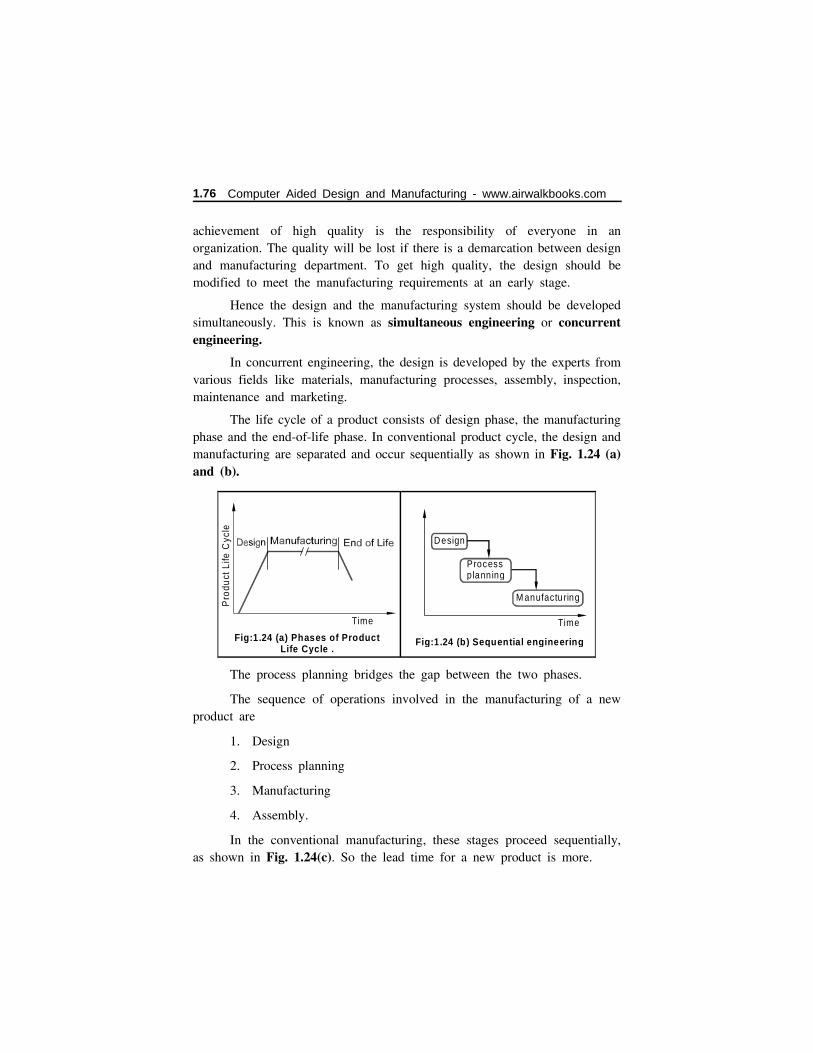
achievement of high quality is the responsibility of everyone in anorganization. The quality will be lost if there is a demarcation between designand manufacturing department. To get high quality, the design should bemodified to meet the manufacturing requirements at an early stage.

Hence the design and the manufacturing system should be developedsimultaneously. This is known as simultaneous engineering or concurrentengineering.

In concurrent engineering, the design is developed by the experts fromvarious fields like materials, manufacturing processes, assembly, inspection,maintenance and marketing.

The life cycle of a product consists of design phase, the manufacturingphase and the end-of-life phase. In conventional product cycle, the design andmanufacturing are separated and occur sequentially as shown in Fig. 1.24 (a)and (b).

The process planning bridges the gap between the two phases.

The sequence of operations involved in the manufacturing of a newproduct are

1. Design

2. Process planning

3. Manufacturing

4. Assembly.

In the conventional manufacturing, these stages proceed sequentially,as shown in Fig. 1.24(c). So the lead time for a new product is more.

Fig:1.24 (b) Sequential engineering

Time

Design

Processplanning

M anufactu ring

Time

Pro

duct

Life

Cyc

le

Fig:1.24 (a) Product Life Cycle .

Phases of


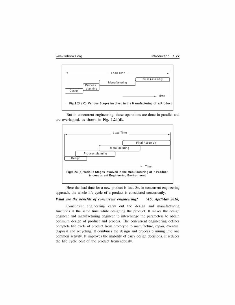
But in concurrent engineering, these operations are done in parallel andare overlapped, as shown in Fig. 1.24(d)..

Here the lead time for a new product is less. So, in concurrent engineeringapproach, the whole life cycle of a product is considered concurrently.

What are the benefits of concurrent engineering? (AU. Apr/May 2018)

Concurrent engineering carry out the design and manufacturingfunctions at the same time while designing the product. It makes the designengineer and manufacturing engineer to interchange the parameters to obtainoptimum design of product and process. The concurrent engineering definescomplete life cycle of product from prototype to manufacture, repair, eventualdisposal and recycling. It combines the design and process planning into onecommon activity. It improves the inability of early design decisions. It reducesthe life cycle cost of the product tremendously.

Tim e

D esign

Process p lann ing

Fina l Assem b ly

Fig:1.24 ( C) Various Stages involved in the Manufacturing of a P roduct

Lead T im e

Lea d T im e

Tim e

D esign

Process planning

M anufac tu ring

Fina l Assem b ly

Fig:1 .24 (d) Various Stages involved in the Manufacturing of a Product in concurrent Engineering Environment


The concept of concurrent engineering is shown in Fig. 1.24(e).In this, the design coordinator coordinates the suggestions from all the

experts of various departments around him.

The design coordinator moves the new design to all the experts. Theexperts discuss it and suggest design changes. The design is then passed backto the design coordinator. He accepts the suggestions, modifies the designand sends it to the experts again for evaluation. On each integration, therewill be fewer and fewer changes and finally optimum design is arrived.

Design for Manufacture and Assembly DFMA

DFM means design of product for ease of manufacture.

DFA means design of product for ease of assembly.

Design for manufacture and assembly means that design the productfor ease of manufacture and for ease of assembly.

i.e. Design a component so that it can be easily manufactured andeasily assembled.

It is the integration of product design, assembly and process planninginto one common activity. It is one of the techniques for applying ConcurrentEngineering.

M arke tingD epartm en t

Sa lesD epartm en t

InspectionD epartm en t

M anufactu ringD epartm en t

Serv iceD epartm en t

Assem blySection

PackagingD epartm en t

Function

Comm un ica tion

C om munication

Fig:1.24 (e) The concept of concurrent engineering


The following are important points to be noted during design formanufacturing and assembly.

1. Number of parts to be designed should be minimum.

2. Variation of part should be minimised.

3. The parts designed should be used for so many functions.

4. Design a part so that it can be easily fabricated.

5. Avoid separate fasteners.

6. Design the part so that it can be easily assembled.

7. Evaluate assembly methods.

8. Avoid flexible components which are difficult to handle.

9. Trade with known and experienced vendors and suppliers.

10. Minimise subassemblies.

11. New technology should not be used unless it is necessary.

12. Emphasize standardization.

13. Use the simple and possible operations.

14. Minimize set up procedures and interventions.

The DFMA reduces the time spent on the design process. Thefollowing Fig. 1.24(f) shows the steps taken for concurrent engineering usingDFMA during design.

In this, the DFA analysis is conducted at first to simplify the productstructure.

By this, early cost estimates for the products are obtained for bothoriginal design and new design and decide which one is economical. Duringthis process, the best materials and best processes are selected for the variousparts of the product. Suggestions for more economic materials and processesare taken into account at this stage. Once the best materials and processesare finalised, a thorough analysis about design for manufacturing (DFM) canbe carried out. By this DFM, the detailed design of parts are evaluated. Thenprototype can be developed and tested. Finally the product will bemanufactured.


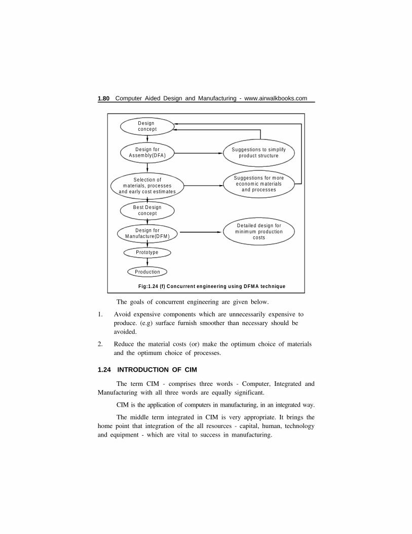
The goals of concurrent engineering are given below.

1. Avoid expensive components which are unnecessarily expensive toproduce. (e.g) surface furnish smoother than necessary should beavoided.

2. Reduce the material costs (or) make the optimum choice of materialsand the optimum choice of processes.

1.24 INTRODUCTION OF CIM

The term CIM - comprises three words - Computer, Integrated andManufacturing with all three words are equally significant.

CIM is the application of computers in manufacturing, in an integrated way.

The middle term integrated in CIM is very appropriate. It brings thehome point that integration of the all resources - capital, human, technologyand equipment - which are vital to success in manufacturing.

D esign concep t

D esign fo rAssem bly(D FA )

Se le ct io n o f m aterials, processes

and ea rly co st estim ates

Be st D e signconcep t

D esign fo rM an ufac tu re(D FM )

Pro to type

Production

Su ggestions to s im plifyp rod uct structu re

Su ggestions fo r m oreecono m ic m ateria ls

and processes

D eta iled design fo rm in im um production

costs

Fig:1.24 (f) Concurrent engineering using DFM A technique


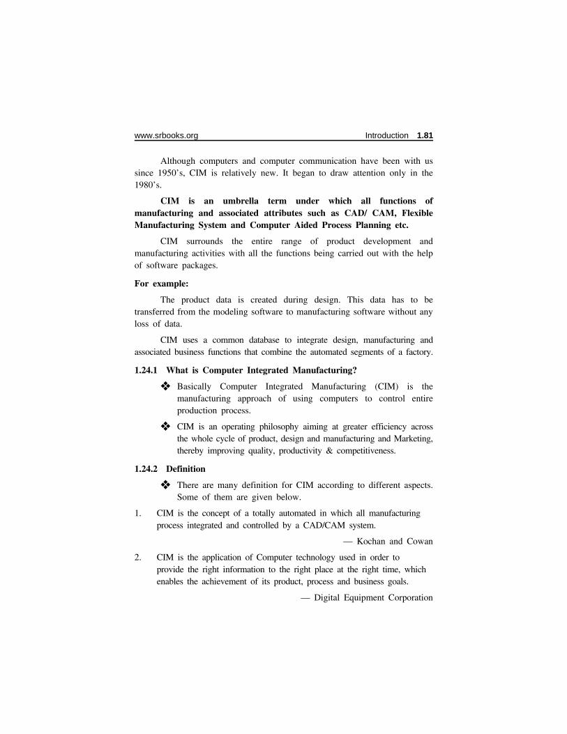
Although computers and computer communication have been with ussince 1950’s, CIM is relatively new. It began to draw attention only in the1980’s.

CIM is an umbrella term under which all functions ofmanufacturing and associated attributes such as CAD/ CAM, FlexibleManufacturing System and Computer Aided Process Planning etc.

CIM surrounds the entire range of product development andmanufacturing activities with all the functions being carried out with the helpof software packages.

For example:

The product data is created during design. This data has to betransferred from the modeling software to manufacturing software without anyloss of data.

CIM uses a common database to integrate design, manufacturing andassociated business functions that combine the automated segments of a factory.

1.24.1 What is Computer Integrated Manufacturing?

❖ Basically Computer Integrated Manufacturing (CIM) is themanufacturing approach of using computers to control entireproduction process.

❖ CIM is an operating philosophy aiming at greater efficiency acrossthe whole cycle of product, design and manufacturing and Marketing,thereby improving quality, productivity & competitiveness.

1.24.2 Definition

❖ There are many definition for CIM according to different aspects.Some of them are given below.

1. CIM is the concept of a totally automated in which all manufacturingprocess integrated and controlled by a CAD/CAM system.

— Kochan and Cowan

2. CIM is the application of Computer technology used in order toprovide the right information to the right place at the right time, whichenables the achievement of its product, process and business goals.

— Digital Equipment Corporation


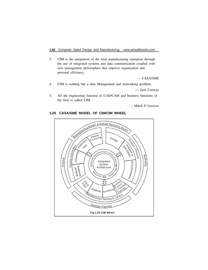
3. CIM is the integration of the total manufacturing enterprise throughthe use of integrated systems and data communication coupled withnew management philosophies that improve organization andpersonal efficiency.

— CASA/SME

4. CIM is nothing but a data Management and networking problem.

— Jack Conway

5. All the engineering function of CAD/CAM and business functions ofthe firm is called CIM.

– Mikill P Groover

1.25 CASA/SME MODEL OF CIM/CIM WHEEL

Fig:1.25 CIM W heel

In tegra te d Sys tem

Arch itecture Res

o urc

e s M

anu facturing & Communica tio n Inform

ation

M ate ria l

P rocessing

Ass

embl

yIn

sp

ec tion

Test

D es ign

Ana lysis &

S imulatio n

Mat

eria

l

Han

dlin

gD

ocumentation

ShopF loor

M ateria l S ch edu ling Q uan ti ty

P rocess

& Fac ilit ies

P lan ning

S trategic P lanning

Manufac tu ring M G M T & H um an R esoures M G M T

Ma rketin

gF

ina

nce

P roduct / Pro ces s


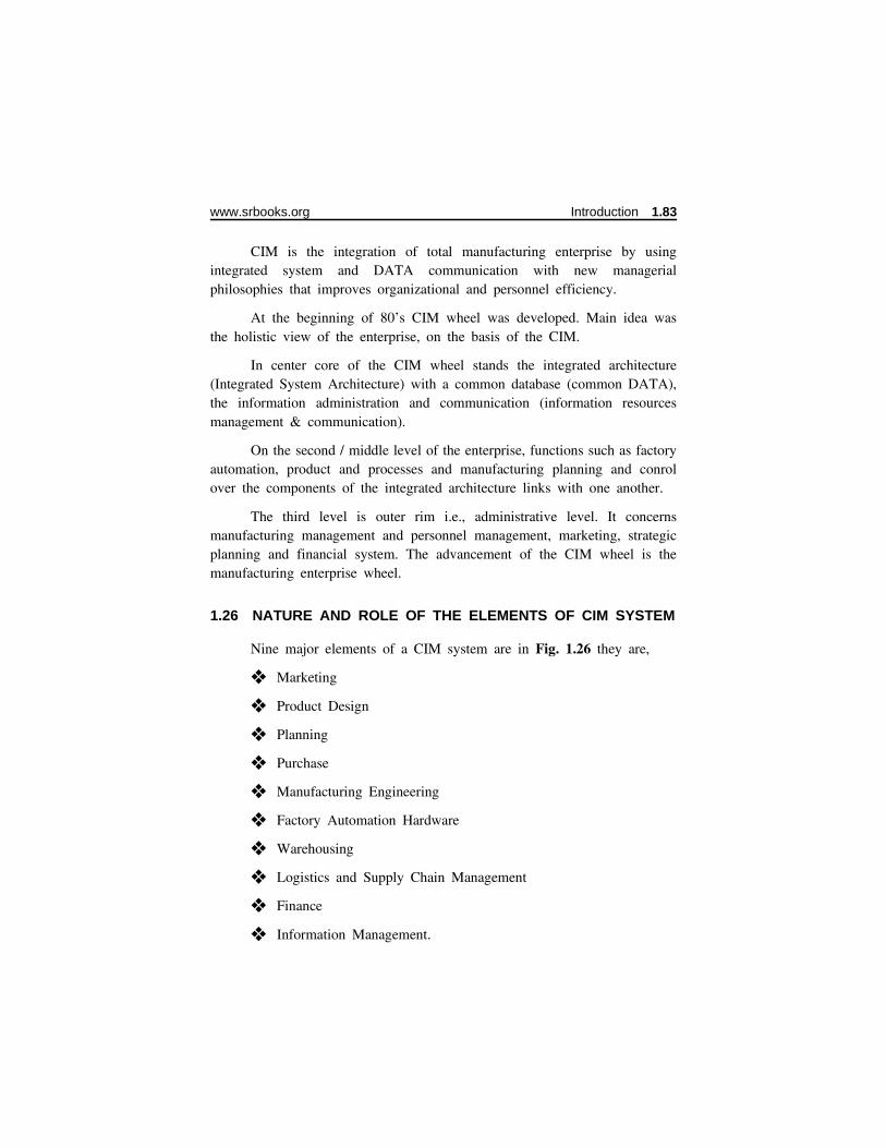
CIM is the integration of total manufacturing enterprise by usingintegrated system and DATA communication with new managerialphilosophies that improves organizational and personnel efficiency.

At the beginning of 80’s CIM wheel was developed. Main idea wasthe holistic view of the enterprise, on the basis of the CIM.

In center core of the CIM wheel stands the integrated architecture(Integrated System Architecture) with a common database (common DATA),the information administration and communication (information resourcesmanagement & communication).

On the second / middle level of the enterprise, functions such as factoryautomation, product and processes and manufacturing planning and conrolover the components of the integrated architecture links with one another.

The third level is outer rim i.e., administrative level. It concernsmanufacturing management and personnel management, marketing, strategicplanning and financial system. The advancement of the CIM wheel is themanufacturing enterprise wheel.

1.26 NATURE AND ROLE OF THE ELEMENTS OF CIM SYSTEM

Nine major elements of a CIM system are in Fig. 1.26 they are,

❖ Marketing

❖ Product Design

❖ Planning

❖ Purchase

❖ Manufacturing Engineering

❖ Factory Automation Hardware

❖ Warehousing

❖ Logistics and Supply Chain Management

❖ Finance

❖ Information Management.


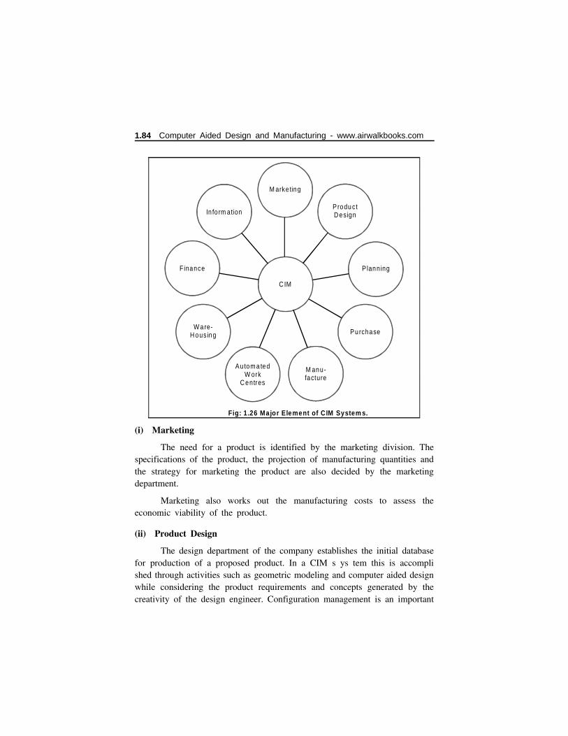
(i) Marketing

The need for a product is identified by the marketing division. Thespecifications of the product, the projection of manufacturing quantities andthe strategy for marketing the product are also decided by the marketingdepartment.

Marketing also works out the manufacturing costs to assess theeconomic viability of the product.

(ii) Product Design

The design department of the company establishes the initial databasefor production of a proposed product. In a CIM s ys tem this is accomplished through activities such as geometric modeling and computer aided designwhile considering the product requirements and concepts generated by thecreativity of the design engineer. Configuration management is an important

In fo rm ation

M arke ting

F inance

C IM

Planning

W are-H ousing

Au tom a tedW ork

C entres

M anu-facture

Purchase

Fig: 1 .26 Major Element of C IM System s.

Produ ctD esign


activity in many designs. Complex designs are usually carried out by severalteams working simultaneously, located often in different parts of the world.The design process is constrained by the costs that will be incurred in actualproduction and by the capabilities of the available production equipment andprocesses. The design process creates the database required to manufacturethe part.

(iii) Planning

The planning department takes the database established by the designdepartment and enriches it with production data and information to producea plan for the production of the product. Planning involves severalsubsystems dealing with materials, facility, process, tools, manpower,capacity, scheduling, outsourcing, assembly, inspection,logistics etc. In aCIM system, this planning process should be constrained by the productioncosts and by the production equipment and process capability, in order togenerate an optimized plan.

(iv) Purchase

The purchase departments is responsible for placing the purchase ordersand follow up, ensure quality in the production process of the vendor, receivethe items, arrange for inspection and supply the items to the stores or arrangetimely delivery depending on the production schedule for eventual supply tomanufacture and assembly.

(v) Manufacturing Engineering

Manufacturing Engineering is the activity of carrying out theproduction of the product, involving further enrichment of the database withperformance data and information about the production equipment andprocesses. In CIM, this requires activities like CNC programming, simulationand computer aided scheduling of the production activity. This should includeonline dynamic scheduling and control based on the real time performanceof the equipment a nd process es to as sure continuous production activity.Often, the need to meet fluctuating market demand requires the manufacturingsystem flexible and agile.


(vi) Factory Automation Hardware

Factory automation equipment further enriches the database withequipment and process data, resident either in the operator or the equipmentto carry out the production process. In CIM system, this consists of computercontrolled process machinery such as CNC machine tools, flexiblemanufacturing systems (FMS). Computer controlled robots, material handlingsystems, computer controlled assembly systems, flexibly automated inspectionsystems and so on.

(vii) Warehousing

Wa rehous ing is the function involving s torage and retrieval of rawmaterials, components, finished goods as well as shipment of items. In today’scomplex outsourcing scenario and the need for just-in-time supply ofcomponents and subsystems, logistics and supply chain management assumegreat importance.

(viii) Finance

Finance deals with the resources pertaining to money. Planning ofinvestment, working capital, and cash flow control, realization of receipts,accounting and allocation of funds are the major tasks of the financedepartments.

(ix) Information Management

Information Management is perhaps one of the crucial tasks in CIM.This involves master production scheduling, database management,communication, manufacturing systems integration and managementinformation systems.

1.9 REASONS FOR IMPLEMENTING CIM

1. To solve following issues

(a) Strategic issue (Lack of information, technologies)

(b) Organization issue (Absence of total management system)

(c) Behavioural issue (Safety, Lack human involvement of CIM)

(d) Technological issues (Incompatible Computer System, short lead life,Frequent job changes)


2. To coordinate and organise data

CIM used for various datas

(i.e.) (i) Functional data

(ii) Product data

(iii) Operational data

(iv) Performance data etc.

3. To meet competitive pressures

Any organization to survive successfully, needs to face the followingcompetitive pressures

(i) Increased quality.

(ii) Reduced production, material & labour cost.

(iii) Reduce inventory.

4. To facilitate Simultaneous Engineering

❖ Concurrent (or) simultaneous engineering is a technology ofrestructuring the product development.

❖ Simultaneous Engineering can be easily implement with the CIM.

1.28 OBJECTIVES/GOAL OF CIM

The main objective are:

(i) More productivity and efficiency of the product.

(ii) More readability.

(iii) Cost of production, maintenance decreases

(iv) To reduce number of hazardous job.

(v) To eliminate human error.

(vi) To increase quality of product.


1.29 CIM I Vs CIM II

CIM I - It refers to Computer Interfaced Manufacturing

CIM II - It refers to Computer Integrated Manufacturing. The concepthas moved from interfacing to Integrating because of the advent ofdevelopments in Computer and Communication Technologies.

❖ The first three generations of computer’s uses vacuum tubes,transistor and Integrated Circuits (IC) etc.

❖ The fourth generation of computers in CIM I used LSI/VLSI(Large scale Integration/very large scale integration) withinterfacing the data.

❖ The fifth generation of computers in CIM II used parallelprocessing with networking environment.

Nowadays the term CIM I and CIM II are not used; Instead the termCIM is used.

Difference between CIM I & CIM II

CIM I Vs CIM II

1. Computer InterfacedManufacturing

Computer IntegratedManufacturing.

2. Interfacing Existing System Integration of total manufacturingenterprises

Fourth generation Computers Fifth generation Computers

1.30 BENEFITS OF CIM

The following is the list of a few benefits that can be achieved byusing CIM.

1. CIM improves the operational control by means of reduction in thenumber of uncontrollable variables, reducing dependents on humancommunication.

2. CIM improves the short run responsiveness.

3. CIM improves long run accommodations by means of changingproduct volumes.


4. CIM reduces the inventory through reducing lot sizes, improvinginventory turnover for the particular company.

5. Better quality in manufacturing products.

6. More accuracy in financial projections and improved cash flow.

7. It helps quicker design & development.

8. Faster access to currentand past product information.

9. CIM increases machine utilizations by means of eliminating (or)reducing machine setup, utilizing automated features.

1.31 COMPUTER INTEGRATED MANUFACTURING (CIM) AS A CONCEPT AND A TECHNOLOGY

A number of definitions have been developed for computer integratedmanufacturing (CIM). However a CIM system is commonly thought of as anintegrated system that compares all the activities in the production systemfrom the planning and design of a product through the manufacturing system,including control. CIM is an attempt to combine existing computertechnologies in order to manage and control the entire business.

A s wit h traditi onal manufacturing approaches, the purpose of CIMis to transform product designs and materials in to salable goods at aminimum cost in the shortest possible time. CIM begins with the design ofa product (CAD) and ends with the manufacture of the product (CAM). WithCIM, the customary split between the design and the manufacturing functionsis (supposed to be) eliminated.

CIM differs from the traditional job shop manufacturing system in therole of the computer plays on the manufacturing process. Computer integratedmanufacturing system are basically a network of computer system tiedtogether by a single integrated database. Using the information in the database,a CIM system can direct manufacturing, distribution and financial functionsinto one coherent system.


1.32 COMPUTERISED ELEMENTS OF A CIM-SYSTEM

CIM Includes

❖ Design parts/products

❖ Planning & control

❖ Automation

❖ Testing

The concept of CIM is to integrate information from Marketing,accounting, planning, control and so on as shown in Fig. 1.27.

❖ The main purpose of CIM is to enable the company to transformideas into a high quality of products in the minimum time, costand CIM goes beyond the scope of FMS (or) CAD/CAM system.

❖ Network and integrated systems are tied up with CIM technologies.

Fig: 1.27 Com puterized Elem ents of a CIM System.

Fac toryO pera tions M

fg.

Pla

nnin

g

Bus

ines

s F

unct

ions

M fgC ontro l

D esign

C AMC os t E stim ation C A PPN C P art Prog ram m ingC om puterized W ork S tds M R P C apa city P lanning

C om puterized Busine ss System s

-O rder Entry-Accou nting-Payroll-Cu stom er B illing

C AMProcess C on tro l P rocess M on ito rin gShop F loo r C on tro l C om puter-aided Inspectio n

C ADG eom etric M ode ling Engine ering A na lysisD esign R eview and Evalu a tionAu tom ated D rafting


❖ The integration of data in CIM allows CAD system to link withNumerical Control, Computer Aided Manufacturing (CAM), Partprograms, Manufacturing Control and Manufacturing planning.

❖ CIM can also be linked with the automatic material handlingsystems to facilitate material handling.

❖ Fully completed integrated system in CIM are not only automatedbut also integrated with each other and also integrated withmanufacturing planning, control and scheduling.

1.33 TYPES OF PRODUCTION

Depending upon the quantities produced in a factory, the productionsystem can be classified into three types

(i) Job shop production (low production)

(ii) Batch production (medium production)

(iii) Mass production (high production)

Fig. 1.28 shows the relation between production quantity Vs productvariety for different production system.

Job Shop

FixedPositionLayou t Process

Layou t

C e llu la rLayou t

ProductLayou t

100 10,000 1 ,000,000

Ba tchProduction

C e llu la r M anufactu rin g

Q uan tity F low L ine

M ass Production

Production Q uantity

Pro

duct

Var

iety

Fig:1. 28


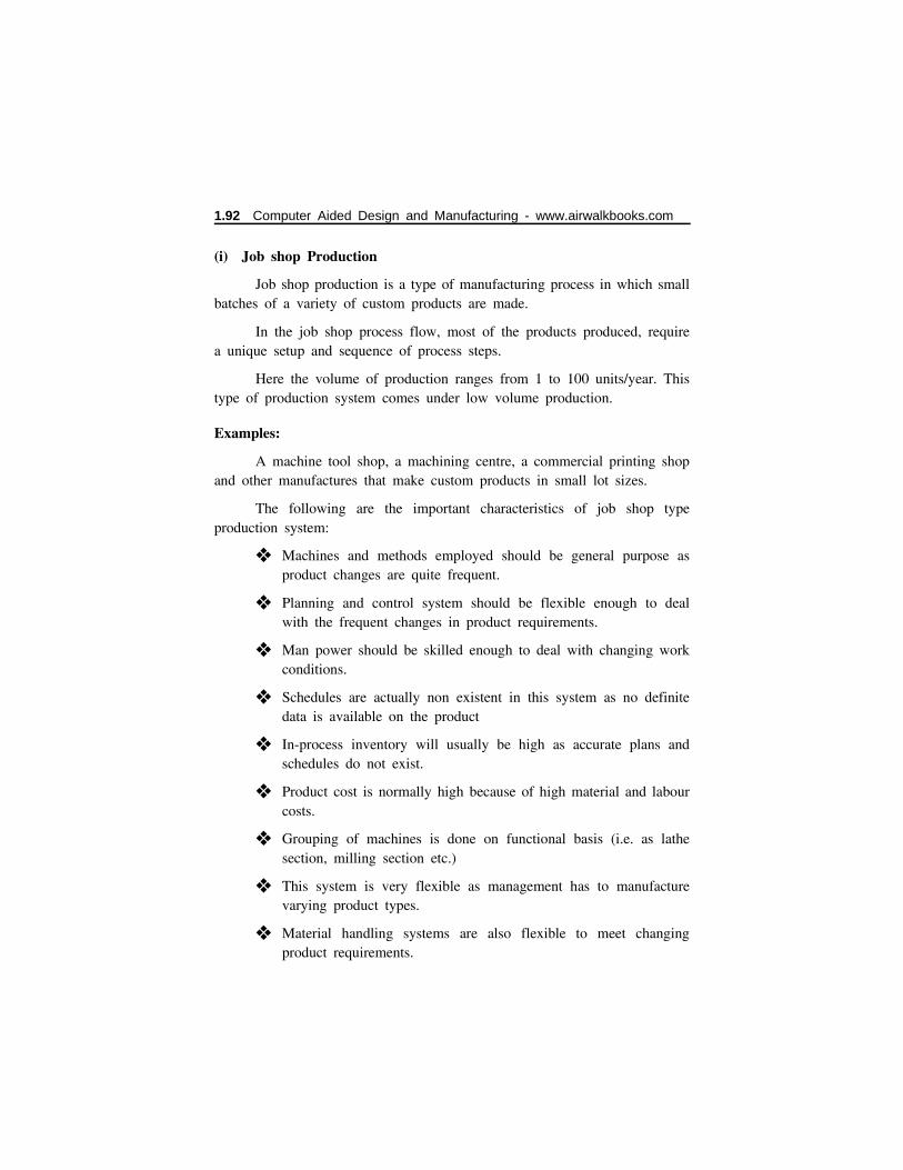
(i) Job shop Production

Job shop production is a type of manufacturing process in which smallbatches of a variety of custom products are made.

In the job shop process flow, most of the products produced, requirea unique setup and sequence of process steps.

Here the volume of production ranges from 1 to 100 units/year. Thistype of production system comes under low volume production.

Examples:

A machine tool shop, a machining centre, a commercial printing shopand other manufactures that make custom products in small lot sizes.

The following are the important characteristics of job shop typeproduction system:

❖ Machines and methods employed should be general purpose asproduct changes are quite frequent.

❖ Planning and control system should be flexible enough to dealwith the frequent changes in product requirements.

❖ Man power should be skilled enough to deal with changing workconditions.

❖ Schedules are actually non existent in this system as no definitedata is available on the product

❖ In-process inventory will usually be high as accurate plans andschedules do not exist.

❖ Product cost is normally high because of high material and labourcosts.

❖ Grouping of machines is done on functional basis (i.e. as lathesection, milling section etc.)

❖ This system is very flexible as management has to manufacturevarying product types.

❖ Material handling systems are also flexible to meet changingproduct requirements.


(ii) Batch production

Batch production is defined by American Production and InventoryControl Society (APICS) “as a form of manufacturing in which the job passesthrough the functional departments in lots or batches and each lot may havea different routing.”

Here the volume of production ranges from 100 - 10,000 units/year.This production system is justified by medium volume production.

Examples:

Electrical goods, newspaper, books etc.

The following are the important characteristics of batch type productionsystem:

❖ As final product is some what standard and manufactured inbatches, economy of scale can be availed to some extent.

❖ Machines are grouped on functional basis similar to the job shopmanufacturing.

❖ Semi automatic, special purpose automatic machines are generallyused to take advantage of the similarity among the products.

❖ Labour should be skilled enough to work up on different productbatches.

❖ In-process inventory is usually high owing to the type of layoutand material handling policies adopted.

❖ Semi automatic material handling systems are most appropriate inconjunction with the semi automatic machines.

❖ Normally production planning and control is difficult due to theodd size and non repetitive nature of order.

(iii) Mass Production

Mass production refers to the process of creating large number ofsimilar products efficiently.

This production system is justified by very large volume of production(i.e. 10,000 to millions of units per year).


Manufacturing of cars and guns are the few examples of massproduction.

The following are the important characteristics of mass productionsystem:

❖ As same product is manufactured for sufficiently long time,machines can be laid down in order of processing sequence.Product type layout is most appropriate for mass productionsystem.

❖ Standard methods and machines are used during part manufacture.

❖ Most of the equipments are semi automatic or automatic in nature.

❖ Material handling is also automatic (such as conveyors).

❖ Semi skilled workers are normally employed as most of thefacilities are automatic.

❖ As product flows along a pre defined line, planning and controlof the system is much easier.

❖ Cost of production is low owing to the high rate of production.

❖ In-process inventories are low as production scheduling is simpleand can be implemented with ease.

1.34 MANUFACTURING MODELS AND METRICS

Many successful manufacturing companies use a variety of metrics tohelp their operations. Generally quantative metrics provide a company withthe means.

(i) To track performance in successive periods.

(ii) Try out new technologies and new systems to determine their merits,identify problems with performance.

(iii) To compare alternative methods and to make good decisions.

The two basic categories of manufacturing metrics are

(i) Production performance measures.

(ii) Manufacturing costs.


Metrics that specify production performance include proportion uptime(or) equipment (a reliability measure), production rate, plant capacity andmanufacturing lead time.

Manufacturing costs in a company includes material and labour cost,the costs of producing its products and the cost of operating a given pieceof equipment.

1.35 MATHEMATICAL MODELS OF PRODUCTION PERFORMANCE

Many features of manufacturing are quantitative. Mathematical modelsof production performance includes production rate, production capacity,utilization & availability and manufacturing lead time.

1.35.1 Production Rate

Production rate for an individual processing is the number of goodsthat can be produced during a given period of time (i.e. work unitscompleted/hr (or) piece/hr). Production rate is determined for the three typesof production systems.

(i) Batch production (ii) Job shop production, (iii) Mass production.For studying the above production process, we must know some basicterminology.

Cycle Time

The period of time spent to complete one cycle of an operation (or)to complete a job from start to finish is called cycle time. It is given by

Tc = T0 + Th + Tth ...(1.26)

where

Tc → cycle time (min/piece)

Th → handling time (min/piece)

T0 → time of the actual processing (min/piece)

Tth → tool handling time (min/piece)


1. Batch and Job shop production

In batch production, the time to process one batch consisting of Nwork units is the sum at the setup time and processing time. It is given by

Tb = Tsu + NTc ...(1.27)

Tb → batch processing time (min)

Tsu → setup time to prepare for the batch (min)

N → batch quantity (piece)

If more than one part is produced in each cycle, the average productiontime per work unit, Tp is given by

Tp = TbN ...(1.28)

and the average production rate is given by

Rp = 60Tp ...(1.29)

where,

Rp → hourly production rate (pc/hr)

Tp → average production time/minute

and the constant 60 converts minutes to hours.

Job Shop Production

When N = 1 the production time per work unit is the sum of setupand cycle times.

Tp = Tsu + Tc ...(1.30)

If N > 1, the production rate is determined as in batch production casediscussed above


Mass Production

For quantity type mass production, the production rate is equal to thecycle rate of the machine (reciprocal of operation cycle time). Here the effect

of setup time is insignificant i.e. N becomes large, (Tsu/N) → 0.

Rp = Rc = 60Tc ...(1.31)

Rc → operation cycle rate of the machine (pc/hr).

For flow line mass production, the operation of production line iscomplicated by interdependence of the workstations on the line. Thereforesome station require longest operation time and this station sets the pace forthe entire line. The term bottleneck station is used to refer to this station.Therefore the cycle time of a production line is given by

Tc = Tr + Max T0 ...(1.32)

Tr → time to transfer work units between each cycle (min/cycle)

Max T0 → operation time at the bottleneck station.

The production rate is given by

Rc = 60Tc ...(1.33)

1.35.2 Production capacity

Production capacity is defined as the maximum rate of output that aproduction facility is able to produce under a given operating conditions.Operating conditions refer to the number of shift/day (or) number of days inthe week that the plant operates. The production capacity can be determinedby the following equation

PC = n Sw Hsh Rc ...(1.34)


where,

PC = Weekly production capacity of the facility (output units/wk)

n = number of work centers * working in parallel producing in the facility

Sw = number of shifts/period (shift/wk)

Hsh = hr/shift (hr)

Rp = production rate of each work center

Note:

*Work center is a manufacturing system in the plant typicallyconsists of one worker and one machine. It might also be automated withno worker (or) multiple workers working together on a production line.It is capable of producing at a rate Rp units/hr.

If we include the possibility that, each work unit requires n0 operations

in its processing sequence, with each operation requiring a new setup oneither the same (or) different machine, then the plant capacity is given by

PC = nsw Hsh Rp

n0 ...(1.35)

where

n0 = no. of distinct operations through which work units are routed.

❖ Changes that can be made to increase (or) decrease plant capacityover short term are

1. Change the number of shifts per week

2. Change the number of hours worked per shift.

❖ To increase plant capacity over longer term work unit by usingcombined operations (or) simultaneous operations.


1.35.3 Utilization

Utilization refers to the amount of output of a production facilityrelative to its capacity. It is usually expressed as a percentage.

U = NPC

N → actual quantity produced by the facility during a given time period (i.e. piece/wk)

U → utilization of the facility.

PC → production capacity for the same period (piece/wk)

1.35.4 Availability

Availability is a common measure of reliability for equipment. It isespecially appropriate for automated production equipment. It is defined usingtwo other reliability terms (i.e.) mean time between failures (MTBF) and meantime to repair (MTTP).

A = MTBF − MTTR

MTBF ...(1.37)

where,

MTBF is the average length of time the piece of equipment runs betweenbreakdowns (i.e. mean time between failures (hr).)

MTTR is the average time required to service the equipment and put it backinto operation when a breakdown occurs [i.e. mean time repair (hr)]

1.17.5 Manufacturing lead time

Manufacturing lead time is the time period between the placement ofan order and the shipment of the completed order to the customer.

A short manufacturing lead time is a competitive advantage to themanufacturing firm because many customers want the delivery of theirproducts as soon as possible following the placement of the order.


❖ For batch production the manufacturing lead time (MLT) is givenby

MLT = n0 (Tsu + NTc + Tno) ...(1.38)

where

n0 = number of separate operations through which the work unit must

be routed.

Tsu = Setup time

Tno = non-operation time of a machine

During batch production, the term N, Tsu, Tc, and Tno would vary for

every product and operation.

The above equation can be adapted for job shop production and massproduction by making adjustments in the parameter values. For job shop, in

which the batch size (N = 1), the equation becomes

MLT = n0 (Tsu + Tc + Tno) ...(1.39)

For mass production, the N − term in Eq. (1.38) is very large anddominates the other terms. In the case of quantity type mass production in

which a large number of units are made on a single machine (n0 = 1), the

MLT simply becomes the operation cycle time for the machine after the setuphas been completed and production begins.

For flow in the mass production, the entire production line is set upin advance. Also, the non-operation time between processing steps is simplythe transfer time Tr to move the part or product from one workstation to the

next. If the workstations are integrated so that all stations are processing theirown respective work unit, then the time to accomplish all of the operationsis the time it takes each work unit to progress through all of the stations onthe line. The station with the longest operation time sets the pace for allstations.

MLT = n0 (Tr + Max To) = no Tc ...(1.40)


where

MLT = time between start and completion of a given work unit on the line (min)

n0 = number of operations on the line

Tr = transfer time (min)

Max To = operation time at the bottleneck station (min) and

Tc = cycle time of the production line (min/piece)

Tc = Tr + Max To from Eq. (1.32). Since the number of stations is equal

to the number of operations (n = no). Equ. (1.40) can also be stated as

MLT = n (Tc + Max To) = n Tc ...(1.41)

where the symbols have the same meaning as above, and we have substitutedn (number of workstations or machine) for number of operations n0.

1.35.6 Work in-process (WIP)

Work in-process is the quantity of parts (or) products currently locatedin the factory that either are being processed (or) between processingoperations.

WIP is determined by,

WIP = AU (PC) (MLT)

Sw Hsh ...(1.42)

where,

A → availability (%)

U → utilization (%)

PC → production capacity of the facility (piece/wk)

MLT → manufacturing lead time (wk)

Sw → number of shifts/week (shift/wk)

Hsh → hours per shift (hr/shift)


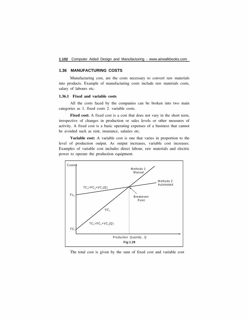
1.36 MANUFACTURING COSTS

Manufacturing cost, are the costs necessary to convert raw materialsinto products. Example of manufacturing costs include raw materials costs,salary of labours etc.

1.36.1 Fixed and variable costs

All the costs faced by the companies can be broken into two maincategories as 1. fixed costs 2. variable costs.

Fixed cost: A fixed cost is a cost that does not vary in the short term,irrespective of changes in production or sales levels or other measures ofactivity. A fixed cost is a basic operating expenses of a business that cannotbe avoided such as rent, insurance, salaries etc.

Variable cost: A variable cost is one that varies in proportion to thelevel of production output. As output increases, variable cost increases.Examples of variable cost includes direct labour, raw materials and electricpower to operate the production equipment.

The total cost is given by the sum of fixed cost and variable cost

C osts

FC 1

Fc2 Bre akeven Po in t

M etho ds 1 :M anua l

M etho ds 2 :Au tomated

TC =FC +VC (Q )2 2 2

TC =FC +VC (Q )1 1 1

VC 1

Fig:1.29

Pro duction Q uan tity , Q


TC = FC + VC (Q) ...(1.43)

TC → TC Total cost

FC → FC Fixed cost

VC → VC Variable cost

Q → Annual quantity produced (piece/yr)

From the graph Fig. 1.29 it is noted that, the fixed cost of theautomated method is high relative to the manual method and variable cost ofautomated method is low relative to the manual method.

1.36.2 Direct labour, Material, and overhead

Manufacturing cost is divided into three broad categories

1. Direct labour cost

2. Direct material cost

3. Manufacturing overhead.

Direct labour cost

The direct labour cost is the sum of the wages and benefits paid tothe workers who operate the production equipment and perform the processingand assembly tasks.

Direct Material Cost

Direct material cost is the cost of the raw materials and componentsused to create a product.

Example: The cost of steel is a direct material in the manufacture ofautomobile.

Overhead Cost

Overhead costs are all of the other expenses associated with runningthe manufacturing firm. Overhead divides into two categories.

1. Factory overhead

Factory overhead consists of the costs of operating the factory otherthan direct labour and materials, such as the factory expenses (i.e. insurance,power for machinery etc.).


The factory overhead rate is calculated as the ratio of factory overheadexpenses to direct labour expenses.

FOHR = FOHCDLC ...(1.44)

FOHR → Factory overhead rate (Rs/yr)

FOHC → Annual factory overhead cost (Rs/yr)

DLC → Annual direct labour costs (Rs/yr)

2. Corporate overhead

It is the cost not related to the company’s manufacturing activities,such as the corporate expenses (i.e. R & D, sales & marketing).

❖ Corporate overhead rate is the ratio of corporate overhead expensesto direct labour expenses.

COHR = COHCDLC ...(1.45)

COHR → Corporate overhead rate (Rs/yr)

COHC → Annual corporate overhead costs (Rs/yr)

DLC → Annual direct labour costs (Rs/yr)

Note:

If material cost are used as the allocation basis, then material costwould be used as the denominator in both ratios

Problem on Production Capacity

Problem 1.11: The turret lathe section has 6 machines all devoted to theoperation of the same part. The section operates 10 shift/wk. The number ofhours / shift averages 8.0. Average production rate of each machine is 17unit/hr. Determine the weekly production capacity of the turret lathe section.

Given:

n = 6

Sw = 10 shift/wk


Hsh = 8 hr/shift

Rp = 17 units/hr

Solution:

PC = nsw Hsh Rp

= 6 × 10 × 8 × 17

= 8160 output unit week

Problem on Utilization

Problem 1.12: A production machine operates 80 hr/wk (2 shifts, 5 days)at full capacity. Its production rate is 20 unit/hr. During a certain week, themachine produced 1000 parts and was idle in the remaining time.(a) Determine the production capacity of the machine. (b) What was theutilization of the machine during the week under consideration?

Solution:

(a) The capacity of the machine can be determined using the assumed80-hr/week as follows:

PC = 80 (20) = 1600 unit wk

(b) Utilization can be determined as the ratio of the number of parts madeby the machine relative to its capacity

U = 1000/1600 = 0.625 (62.5%)

(or)

The alternative way of assessing utilization is by the time during theweek that the machine was actually used. To produce 1000 units, the machinewas operated

H = 1000 pc20 pc/hr

= 50 hr

Utilization is defined relative to the 80 hr available

U = 5080

= 0.625 (62.5 %)


Problem on Effect of Utilization and Availability on Plant Capacity

Problem 1.3: Consider Example 1.1. Suppose the same data from that

example were applicable, but that the availability of the machines A = 90%

and the utilization of the machines U = 80%. Given this additional data,

compute the expected plant output.

Given:

A = 90 % = 0.90

U = 80 % = 0.80

Solution:

Equation (1.34) can be altered to include availability and utilization as

Q = AU (n Sw Hsh Rp)

where A = availability and U = utilization. Combining the previousand new data, we have

Q = 0.90 (0.80) (6) (10) (8.0) (17) = 5875 output units/wk.

Problem on Manufacturing lead time:

Problem 1.14: A certain part is produced in a batch size of 100 units. Thebatch must be routed through five operations to complete the processing ofthe parts. Average setup time is 3 hr/operation and average operation timeis 6 min (0.1/hr). Average non-operation time due to handling, delays,inspections etc. is 7 hrs for each operation. Determine how many days it willtake to complete the batch, assuming the plant runs 8 hr. shift/day.

Given:

N = 100 units

Tsu = 3 hr/operation

Tno = 7 hr/operation

Tc = 0.1 hr

n0 = 5


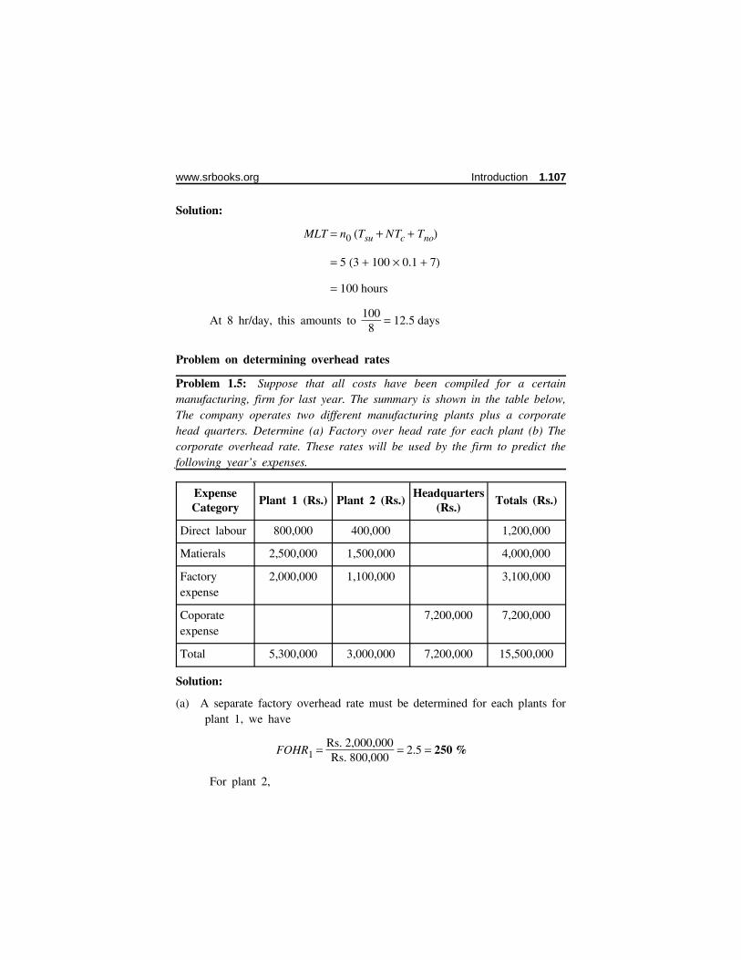
Solution:

MLT = n0 (Tsu + NTc + Tno)

= 5 (3 + 100 × 0.1 + 7)

= 100 hours

At 8 hr/day, this amounts to 100

8 = 12.5 days

Problem on determining overhead rates

Problem 1.5: Suppose that all costs have been compiled for a certainmanufacturing, firm for last year. The summary is shown in the table below,The company operates two different manufacturing plants plus a corporatehead quarters. Determine (a) Factory over head rate for each plant (b) Thecorporate overhead rate. These rates will be used by the firm to predict thefollowing year’s expenses.

ExpenseCategory

Plant 1 (Rs.) Plant 2 (Rs.)Headquarters

(Rs.)Totals (Rs.)

Direct labour 800,000 400,000 1,200,000

Matierals 2,500,000 1,500,000 4,000,000

Factoryexpense

2,000,000 1,100,000 3,100,000

Coporateexpense

7,200,000 7,200,000

Total 5,300,000 3,000,000 7,200,000 15,500,000

Solution:

(a) A separate factory overhead rate must be determined for each plants forplant 1, we have

FOHR1 = Rs. 2,000,000Rs. 800,000

= 2.5 = 250 %

For plant 2,


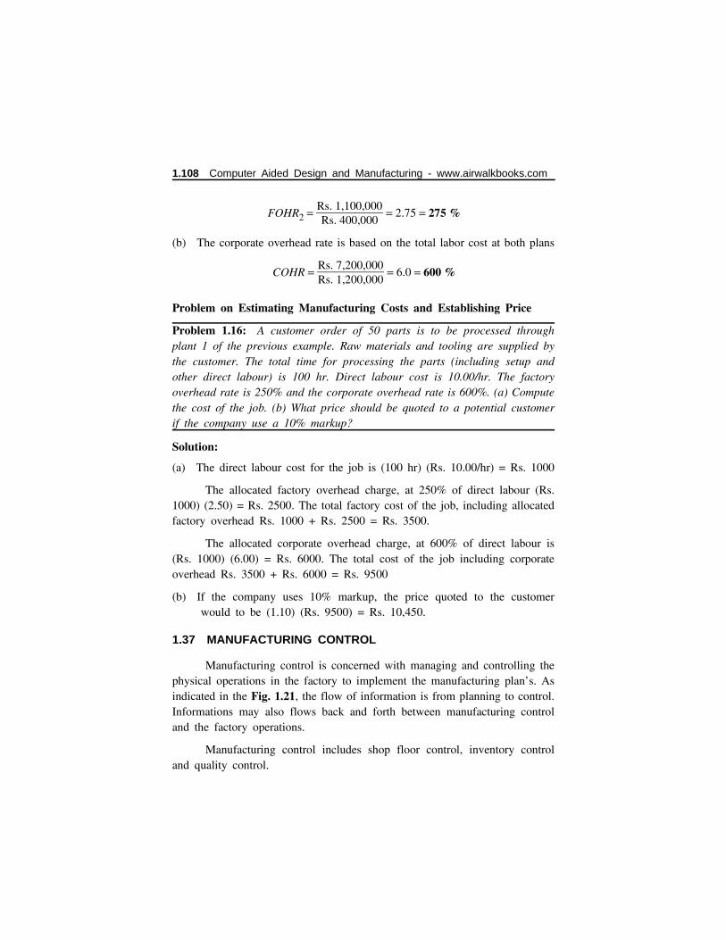
FOHR2 = Rs. 1,100,000Rs. 400,000

= 2.75 = 275 %

(b) The corporate overhead rate is based on the total labor cost at both plans

COHR = Rs. 7,200,000Rs. 1,200,000

= 6.0 = 600 %

Problem on Estimating Manufacturing Costs and Establishing Price

Problem 1.16: A customer order of 50 parts is to be processed throughplant 1 of the previous example. Raw materials and tooling are supplied bythe customer. The total time for processing the parts (including setup andother direct labour) is 100 hr. Direct labour cost is 10.00/hr. The factoryoverhead rate is 250% and the corporate overhead rate is 600%. (a) Computethe cost of the job. (b) What price should be quoted to a potential customerif the company use a 10% markup?

Solution:

(a) The direct labour cost for the job is (100 hr) (Rs. 10.00/hr) = Rs. 1000

The allocated factory overhead charge, at 250% of direct labour (Rs.1000) (2.50) = Rs. 2500. The total factory cost of the job, including allocatedfactory overhead Rs. 1000 + Rs. 2500 = Rs. 3500.

The allocated corporate overhead charge, at 600% of direct labour is(Rs. 1000) (6.00) = Rs. 6000. The total cost of the job including corporateoverhead Rs. 3500 + Rs. 6000 = Rs. 9500

(b) If the company uses 10% markup, the price quoted to the customerwould to be (1.10) (Rs. 9500) = Rs. 10,450.

1.37 MANUFACTURING CONTROL

Manufacturing control is concerned with managing and controlling thephysical operations in the factory to implement the manufacturing plan’s. Asindicated in the Fig. 1.21, the flow of information is from planning to control.Informations may also flows back and forth between manufacturing controland the factory operations.

Manufacturing control includes shop floor control, inventory controland quality control.


❖ Shop floor control

It deals with the problem of monitoring the progress of the product asit is being processed, assembled, moved and inspected in the factory.

Shop floor control is concerned with inventory in the sense that thematerials being processed in the factory are work-in process inventory. Thusthe shop floor control and inventory control overlap to some extent.

❖ Inventory control: attempts to strike a proper balance betweenthe risk of too litte inventory (with possible stock outs of materials)and the carrying cost of too much inventory. It deals with suchissues as deciding the right quantities of materials to order andwhen to reorder a given item when stock is low.

❖ Quality Control: The function of quality control is to ensure thatthe quality of the product and its components meet the standardsspecified by the product designer. To accomplish its mission,quality control depends on inspection activities performed in thefactory at various times during the manufacture of the product.Also, raw materials and component parts from outside sources aresometimes inspected when they are received, and final inspectionand testing of the finished product is performed to ensurefunctional quality and appearance. Quality control also includesdata collection and problem solving approaches to address processproblems related to quality. Examples of these approaches arestatistical process control (SPC) and Six Sigma.


Documents

airwalkbooks.comairwalkbooks.com/images/pdf/pdf_123_1.pdf · Computer Aided Design and Manufacturing (For B.E. / B.Tech Mechanical Engineering Students) As per the Latest Syllabus