Computer Aided Control System Designmaapc/static/files/CACSD/... · 2018-02-07 · ∗AutoCode (automatic generation of C-code) ... Design controllers such that the closed-loop system

'

&

$

%

Control System Design

Computer Aided

Bart De Moor

Koen Eneman

YI Cheng

ESAT–SCD–SISTA, K.U.Leuven

Kasteelpark Arenberg 10, 3001 Leuven, Belgium

Tel: 32-(0)16-32 17 09 Fax: 32-(0)16-32 19 70

ESAT–SCD–SISTA CACSD pag. 1

'

&

$

%

What you should be able to do whenyou have successfully completed this

course . . .

• Plant modeling in state space.

• Defining control specifications.

• Control system analysis.

– Controllability/observability.

– Stability.

– Performance analysis.

– Elementary sensitivity and robustness analysis.

• Controller design.

– State feedback control design.

Pole-placement, LQR.

– Observer design.

Pole-placement, Kalman filter.

– Compensator design.

Separation principle, LQG.

– Reference introduction and tracking.

– Basics of MPC.


'

&

$

%

List of book-references

• Gene F. Franklin, J. David Powell and Abbas Emami-Naeini, Feedback

Control of Dynamic Systems, Third Edition, Addison-Wesley, 1994.

• Gene F. Franklin, J. David Powell and M.L. Workman, Digital Control of

Dynamic Systems, 2nd ed., Addison-Wesley, 1990.

• R. Dorf, Modern Control Systems, 7th ed., Addison-Wesley, 1995.

• M. Green and D.J.N. Limebeer, Linear Robust Control, Prentice Hall, 1995.

• K.J. Astrom and B. Wittenmark, Adaptive Control, Second Edition,

Addison-Wesley, 1995

• A. Saberi, B.M. Chen and P. Sannuti, Loop Transfer Recovery: Analysis

and Design, Springer-Verlag, 1993

• T. Chen and B. Francis, Optimal Sampled-Data Control Systems, Springer,

1995

• R.J. Vaccaro, Digital Control, A State Space Approach, McGraw-Hill, 1995

• L. Ljung and T. Glad, Modelling of Dynamic Systems, Prentice-Hall, 1994

• R.N. Bateson, Introduction to Control System Technology, Fourth Edition,

Merril MacMillan, 1993

• N.S. Nise, Control System Engineering, Second Edition, Benjamin-

Cummings, 1995

• K. Zhou, J.C. Doyle and K. Glover, Robust and Optimal Control, Prentice

Hall, 1995

• . . . don’t hesitate to consult the library (LIBIS) . . .

http://www.libis.kuleuven.ac.be/


'

&

$

%

List of journals

• IEEE Transactions on Automatic Control

• International Journal on Control

• SIAM Journal on Control and Optimization

• Automatica

• European Control Journal

• Journal A

• IEEE Transactions on Control Systems Technology

• . . .


'

&

$

%

List of Conferences

• Benelux Meeting on Systems and Control

• European Control Conference

• American Control Conference

• MTNS: Mathematical Theory of Networks and Systems

• IFAC: World Congress

• IEEE Conference on Decision and Control

• . . .


'

&

$

%

List of organisations

• IEEE (Institute of Electrical and Electronics Engineers), Control

Systems Society

• IFAC (International Federation of Automatic Control)

• BIRA (Belgisch Instituut voor Regeltechniek en Automatisatie)

• Belgian Graduate School on Systems and Control

• ISA (Instrumentation Society of America)

• SIAM (Society for Industrial and Applied Mathematics)

• . . .


'

&

$

%

Software references

• Matlab

– Matlab

– Simulink

– Toolboxes :

∗ Control System

∗ System Identification (some of the algorithms

were developed at ESAT, e.g. N4SID)

∗ MMLE3 Identification

∗ Mu-Analysis and Synthesis

∗ Neural Network

∗ Optimization

∗ Robust Control

∗ Signal Processing

∗ Statistics

∗ Symbolic Math

∗ Extended Symbolic Math

• RaPID (developed at ESAT)


'

&

$

%

• Xmath

– Control Design Module

– Interactive Control Design Module

– Interactive System Identification Module (developed

at ESAT)

– Optimization Module

– Robust Control Module

– Model Reduction Module

– Signal Analysis Module

– Xµ Module

– GUI Module

– SystemBuild

∗ BlockLibrary

∗ AutoCode (automatic generation of C-code)

∗ DocumentIt (automatic documentation of block

diagrams)


'

&

$

%

Control Companies

• Fisher-Rozemount

• Honeywell

• ABB

• Setpoint-IPCOS

• Eurotherm

• Cambridge-Control

• ISI

• Yokogawa

• Siemens

• ISMC (KUL spin-off)

• . . . and many others . . .

Applications

Literally: everywhere, all sectors, all industries, economy,

process industry, mechatronic design, . . . .


'

&

$

%

Chapter 1

Introduction

Control system engineering isconcerned with modifying thebehavior of dynamical systemsto achieve certain pre-specifiedgoals.

Control design loop:

• Modeling:

Physical plants⇒ Mathematical models.

• Analysis:

Given performance specifications, check whether the

specifications are satisfied; Robustness issues.

• Design:

Design controllers such that the closed-loop system sat-

isfies the specifications.


'

&

$

%

Control system design

-sensors

-sampling rates

-filter selection

-data storage

-physical

-black box

-system identification

-parameter estimation

-model validation

Data acquisition

Modeling

(hardware)

“closing the loop”

Plant -system“definition”

informationa priori

constraints

OK!

design & analysis

Controller implementation

spec’s met?

specification

specification

constraints

yes no

Control system


'

&

$

%

3 Motivating Examples

Philips Glass Tube Manufacturing Process

Mandrel Pressure

Mandrel

Glass Tube

Furnace

0 100 200 300 400 500 600 700 800-0.02

0

0.02

0.04

0 100 200 300 400 500 600 700 800-0.04

-0.02

0

0.02

0.04

0 100 200 300 400 500 600 700 800-20

-10

0

10

20

0 100 200 300 400 500 600 700 800-0.1

-0.05

0

0.05

0.1

Melted Glass

Quartz Sand

Input 1

Output 2Thickness

Drawing Speed

Input 2

DiameterOutput 1

Control design specifications: design a controller such that

the wall thickness and diameter are as constant as possible.


'

&

$

%

Modeling via system identification:

informationa priori

disturbance modelMathematical Model

identificationalgorithms

outputsinputs

simulatedpredicted

outputs

disturbance model

disturbances

Plant


'

&

$

%

Plot with simulation and validation results:


'

&

$

%

System identification toolbox

• Xmath GUI identification toolbox.

• Matlab Toolbox of system identification.

• RaPID (some algorithms developed at ESAT/SISTA)

• · · · · · ·


'

&

$

%

After system identification, a 9th order linear discrete-time

model with two inputs and two outputs was obtained:

xk+1 = Axk +Buk + wk,

yk = Cxk +Duk + vk.

E[

wk

vk

][

wTl vTl

]

=

[

Q S

ST R

]

δkl

where A, B, C, D are matrices, uk is the control input

and wk and vk are process noise and measurement noise

respectively.

Control design results:

Filt 1

Filt 2

SetpointDiameter

Setpoint

Thickness

Static

Ffwd

-

-Decoupling

Static

PIID 2

PIID 1Plant

Thickness

Diameter

Controller =

two feedforward filters

a static feedforward controller

a static decoupling controller

two PIID controllers


'

&

$

%

The two PIIDs control the decoupled loops. Parameter

tuning follows from a multi-objective optimization algo-

rithm.

The control design loop for this application :

State space model

Kalman filter

Hardware constraints

Hardwareimplementation

PIID/Static decoupling

Multi-objective optimization

LQG

Static feedback

Controller design


'

&

$

%

Quality improvement via control:

Histogram of the measured diameter and thickness

-0.2 -0.1 0 0.1 0.20

100

200

300Diameter - No Control

-0.2 -0.1 0 0.1 0.20

100

200

300Diameter - PIID Controlled

-0.02 -0.01 0 0.01 0.020

100

200

300

400Thickness - No Control

-0.02 -0.01 0 0.01 0.020

100

200

300

400Thickness - PIID Controlled


'

&

$

%

Boeing 747 aircraft control:

output

Velocity vector β

x,u

αφ,p

θ,q y,v

Aileronz,w

ψ,r

Rudder δr

Elevator δe

input

x, y, z = position coordinates φ = roll angle

u, v, w = velocity coordinates θ = pitch angle

p = roll rate ψ = yaw angle

q = pitch rate β = slide-slip angle

r = yaw rate α = angle of attack


'

&

$

%

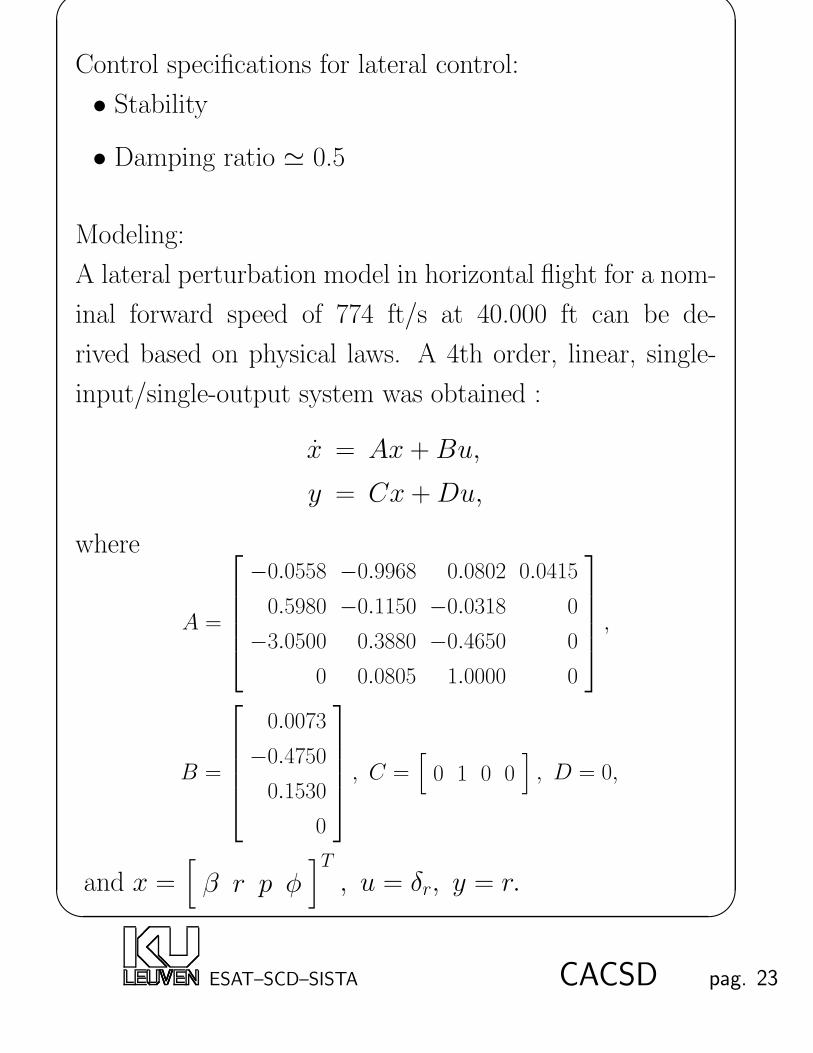
Control specifications for lateral control:

• Stability

• Damping ratio ' 0.5

Modeling:

A lateral perturbation model in horizontal flight for a nom-

inal forward speed of 774 ft/s at 40.000 ft can be de-

rived based on physical laws. A 4th order, linear, single-

input/single-output system was obtained :

x = Ax +Bu,

y = Cx +Du,

where

A =

−0.0558 −0.9968 0.0802 0.0415

0.5980 −0.1150 −0.0318 0

−3.0500 0.3880 −0.4650 0

0 0.0805 1.0000 0

,

B =

0.0073

−0.4750

0.1530

0

, C =[

0 1 0 0]

, D = 0,

and x =[

β r p φ]T

, u = δr, y = r.


'

&

$

%

Control design:

The controller is a proportional feedback from yaw rate to

rudder, designed based on the root-locus method.

δr rerc

−

Rudder

servoAircraft

K

030

Im

Re

stable unstable

damping ratio = 0.5


'

&

$

%

Analysis:

• For good pilot handling, the damping ratio of the sys-

tem should be around 0.5. The open loop system, with-

out control, has a damping ratio of 0.03, far less than

0.5. With the controller, the damping ratio is 0.35, near

to 0.5 : a big improvement !

• Consider the initial-condition response for initial slide-

slip angle β0 = 1 :

0 5 10 15 20 25 30−0.01

−0.005

0

0.005

0.01

0.015

Time (secs)

Response at r to a small initial β

No feedback

Yaw rate feedback

yaw

rater

rad/s

ec


'

&

$

%

Automobile control: CVT control

psc

Output

Rscf

channel

oil pump

cylindersecondary

valvesecondary

Cchc

Csvk

Csck

RsvfNengine

Iscm

Isvm

pcl

Gsvr3 qsv

r3

Gsvr2 qsv

r2

Gsvr1

qsv1

psv1 Input

Csvc1

Csvc2

qsv

vsvm

vscm

Gscr qsc

r

f sc1 Csc

c beltNengine

Nwheel

primary pulley set

secondary pulley set

Ck = spring constant

Im = inertia

R = friction resistor

Gr = hydraulic impedance

p = pressure

q = oil flow

vm = velocity of a mass

f = force


'

&

$

%

Control specifications (tracking problem):

• stability,

• no overshoot,

• steady state error on the step response ≤ 2%,

• rise time of the step response is ≤ 50ms.

Modeling:

A 6th order single-input/single-output nonlinear system

was obtained by physical (hydraulic and mechanical) mod-

eling.

Controller design:

The control problem is basically a tracking problem:

−K P

e psv1 psc

pscref

A PID controller is designed using optimal and robust con-

trol methods.


'

&

$

%

Analysis:

It is required that there is no overshoot and that the rise

time and steady state error of the step time response should

be less than 50 ms and 2% respectively.

Without feedback control: overshoot 20% with oscillation!

With a PID controller: no overshoot, rise time is less than

30ms, no steady-state error.

Step (from 40 bar to 20 bar) responses:

0 0.01 0.02 0.03 0.04 0.05 0.06 0.07 0.08 0.09 0.115

20

25

30

35

40

45

Time:sec.

Pre

ssur

e (b

ar)

Step responses

no feedback control

with a PID controller


'

&

$

%

General Control Configuration

e-Ts

sensor noise

sensor

uncertainty

-Plant

time delayprocessnoise

Cpre

Cff

Ccon1

Ccon2

∆

S

G

v

w

y

uref. e

dist. d

e


'

&

$

%

Systems and Models• Linear - Nonlinear systems

A system L is linear

⇔if input u1 yields output L(u1) and input u2 yields out-

put L(u2), then :

L(c1u1 + c2u2) = c1L(u1) + c2L(u2), c1, c2 ∈ R

In this course, we only consider linear systems.

• Lumped - distributed parameter systems

Many physical phenomena are described mathemati-

cally by partial differential equations (PDEs). Such sys-

tems are called distributed parameter systems. Lumped

parameter systems are systems which can be described

by ordinary differential equations (ODEs).

Example :

– Diffusion equation→ discretize in space

– Heat equation

In this course, we only consider lumped parameter sys-

tems.


'

&

$

%

• Time invariant - time varying systems

A system is time varying if one or more of the param-

eters of the system may vary as a function of time,

otherwise, it is time invariant.

Example: Consider a system

Md2y

dt+ F

dy

dt+Ky = u(t)

If all parameters (M,F,K) are constant, it is time in-

variant. Otherwise, if any of the parameters is a func-

tion of time, it is time varying.

In this course, we only consider time-invariant systems.

• Continuous time - discrete time systems

A continuous time system is a system which describes

the relationship between time continuous signals, and

can be described by differential equations. A discrete

system is a system which describes the relationship be-

tween discrete signals, and can be described by differ-

ence equations.

In this course, we’ll consider systems both in continuous

and discrete time.


'

&

$

%

• Causal - a-causal systems

A system is called causal, if the output to time T de-

pends only on the input up to time T , for every T ,

otherwise it is called a-causal.

In this course, we only consider causal systems.

This course:

Linear

Lumped parameters

Time-invariant

Causal

systems indiscrete time

continuous time

Realistic? In many real cases, YES!

• Industrial processes around an equilibrium point: glass

oven, aircraft and CVT.

• Linearization of a nonlinear system→ linear system.

• . . .


'

&

$

%

System Modeling

System models are developed in two ways mainly:

• Physical modeling consists of applying various laws of

physics, chemistry, thermodynamics, . . . , to derive

ODE or PDE models. It is modeling from “First Prin-

ciples”.

Example:

k

m

F = kx

F = mg (Newton)

md2x

dt2= mg − kx.

• Empirical modeling or identification consists of devel-

oping models from observed or collected data.

Experiments:

− System identification, e.g.: glass oven

− Parameter estimation


'

&

$

%

Chapter 2

State Space Models

General format :

(valid for any nonlinear causal system)

CT : x = f(x, u), DT : xk+1 = f(xk, uk),

y = h(x, u). yk = h(xk, uk).

where

x = the state of the system, n× 1-vector

u = the input of the system, m× 1-vector

y = the output of the system, p× 1-vector

f = state equation vector function

h = output equation vector function

n = number of states⇒ n-th order system

m = number of inputs

p = number of outputs

Single-Input Single-Output system (SISO) : m = p = 1,

Multi-Input Multi-Output system (MIMO) : m, p > 1,

Multi-Input Single-Output system (MISO) :m > 1, p = 1,

Single-Input Multi-Output system (SIMO) :m = 1, p > 1.


'

&

$

%

Linear Time Invariant (LTI) systems(only valid for linear causal systems)

Continuous-time system:

x = Ax +Bu

y = Cx +Du

u Bx x

C

D

A

∫y

Discrete-time system:

xk+1 = Axk +Buk

yk = Cxk +Duk

uk B

xk+1 xk

C

D

A

z−1 yk

A: n× n system matrix

B: n×m input matrix

C: p× n output matrix

D: p×m direct transmission matrix


'

&

$

%

An example of linear state space modeling:

Example: Tape drive control - state space modeling

Process description:

p1 p3 p2

r r

θ1 θ2

K

D

K

D

Kt Kt

ββJ J

i1 i2

+ +

−−e1 e2

The drive motor on each end of the tape is independently

controllable by voltage resources e1 and e2. The tape is

modeled as a linear spring with a small amount of viscous

damping near to the static equilibrium with tape tension

6N. The variables are defined as deviations from this equi-

librium point.


'

&

$

%

The equations of motion of the system are:

capstan 1: Jdω1

dt= Tr − βω1 +Kti1,

speed of x1: p1 = rω1,

motor 1: Ldi1dt

= −Ri1 −Keω1 + e1,

capstan 2: Jdω2

dt= −Tr − βω +Kti2,

speed of x1: p2 = rω2,

motor 2: Ldi2dt

= −Ri2 −Keω2 + e2,

Tension of tape: T =K

2(p2 − p1) +

D

2(p2 − p1),

Position of the head: p3 =p1 + p2

2.


'

&

$

%

Description of variables and constants:

D = damping in the tape-stretch motion

= 20 N/m·sec,e1,2 = applied voltage, V,

i1,2 = current into the capstan motor,

J = inertia of the wheel and the motor

= 4×10−5kg·m2,

β = capstan rotational friction, 400kg·m2/sec,

K = spring constant of the tape, 4×104N/m,

Ke = electrical constant of the motors = 0.03V·sec,Kt = torque constant of the motors = 0.03N·m/A,

L = armature inductance = 10−3 H,

R = armature resistance = 1Ω,

r = radius of the take-up wheels, 0.02m,

T = tape tension at the read/write head, N ,

p1,2,3 = tape position at capstan 1,2 and the head,

p1,2,3 = tape velocity at capstan 1,2 and the head,

θ1,2 = angular displacement of capstan 1,2,

ω1,2 = speed of drive wheels = θ1,2.


'

&

$

%

With a time scaling factor of 103 and a position scaling fac-

tor 10−5 for numerical reasons, the state equations become:

x = Ax +Bu,

y = Cx +Du,

where

x =

p1

ω1

p2

ω2

i1

i2

, A =

0 2 0 0 0 0

−0.1 −0.35 0.1 0.1 0.75 0

0 0 0 2 0 0

0.1 0.1 −0.1 −0.35 0 0.75

0 −0.03 0 0 −1 0

0 0 0 −0.03 0 −1

B =

0 0

0 0

0 0

0 0

1 0

0 1

, C =

[

0.5 0 0.5 0 0 0

−0.2 −0.2 0.2 0.2 0 0

]

,

D =

[

0 0

0 0

]

, y =

[

p3

T

]

, u =

[

e1

e2

]

.


'

&

$

%

State-space model, transfer matrix and impulseresponse

Continuous-time system:

state-space

equations

x = Ax+ Bu

y = Cx+Du

Laplacex(0)=0−→ G(s) =

Y (s)

U(s)= D + C(sI − A)−1B

︸︷︷︸

transfer matrixin practice : D = 0

⇓

G(t) = CeAtB︸︷︷︸

impulse response matrix

Laplace←→ G(s) =∞∑

i=1

CAi−1Bs−i

︸︷︷︸

transfer matrix

Discrete-time system:

state-space

equations

xk+1 = Axk +Buk

yk = Cxk +Duk

z − transfx0=0←→ G(z) =

Y (z)

U(z)= D + C(zI −A)−1B

︸︷︷︸

transfer matrix⇓

G(k) =

D : k = 0

CAk−1B : k ≥ 1︸︷︷︸

impulse response matrix

z − transf←→ G(z) =

∞∑

i=1

CAi−1Bz−i +D

︸︷︷︸

transfer matrix

In case of a SISO system, G(t) or G(k) is the impulse

response.

For MIMO G(t), G(k) are matrices containing the m× pimpulse responses (one for every input-output pair).


'

&

$

%

Linearization of a nonlinear systemabout an equilibrium point

Consider a general nonlinear system in continuous time :

dx

dt= f(x, u)

y = h(x, u)

For small deviations about an equilibrium point (xe, ue, ye)

for which

f(xe, ue) = 0

ye = h(xe, ue)

we define

x = xe + ∆x, u = ue + ∆u, y = ye + ∆y,

and obtain

dx

dt=d∆x

dt= f(x, u) = f(xe + ∆x, ue + ∆u)

and

ye + ∆y = h(x, u) = h(xe + ∆x, ue + ∆u).


'

&

$

%

By first order approximation we obtain a linear state space

model from ∆u to ∆y :

d∆x

dt= f(xe + ∆x, ue + ∆u)

⇓ f(xe, ue) = 0

d∆x

dt

(1)=∂f

∂x

∣∣∣∣xe,ue︸︷︷︸

n× n⇓A

∆x +∂f

∂u

∣∣∣∣xe,ue︸︷︷︸

n×m⇓B

∆u

and

ye + ∆y = h(xe + ∆x, ue + ∆u)

⇓ ye = h(xe, ue)

∆y(1)=∂h

∂x

∣∣∣∣xe,ue︸︷︷︸

p× n⇓C

∆x +∂h

∂u

∣∣∣∣xe,ue︸︷︷︸

p×m⇓D

∆u

Conclusion : use a linear approximation about equilibrium.


'

&

$

%

Example :

Consider a decalcification plant which is used to reduce the

concentration of calcium hydroxide in water by forming a

calcium carbonate precipitate.

The following equations hold (simplified model) :

• chemical reaction : Ca(OH)2 + CO2→ CaCO3 + H2O

• reaction speed : r = c[Ca(OH)2][CO2]

• rate of change of concentration :

d[Ca(OH)2]

dt=k

V− r

V

d[CO2]

dt=u

V− r

V

k and u are the inflow rates in moles/second of calcium

hydroxide and carbon dioxide respectively. V is the tank

volume in liters.

Let the inflow rate of carbon dioxide be the input and the

concentration of calcium hydroxide be the output.


'

&

$

%

A nonlinear state space model for this reactor is :

d[Ca(OH)2]

dt=

k

V− c

V[Ca(OH)2][CO2]

d[CO2]

dt=

u

V− c

V[Ca(OH)2][CO2]

y = [Ca(OH)2]

The state variables are x1 = [Ca(OH)2] and x2 = [CO2].

In equilibrium we have :

k

V− c

V[Ca(OH)2]eq[CO2]eq =

k

V− c

VX1X2 = 0

ueq

V− c

V[Ca(OH)2]eq[CO2]eq =

U

V− c

VX1X2 = 0

Y = [Ca(OH)2]eq = X1

For small deviations about the equilibrium :

d∆x1

dt= − c

VX2∆x1 −

c

VX1∆x2

d∆x2

dt= − c

VX2∆x1 −

c

VX1∆x2 +

1

V∆u

∆y = ∆x1

so,

A =

[

−cX2V−cX1

V

−cX2V−cX1

V

]

, B =

[

01V

]

, C =[

1 0]

, D = 0


'

&

$

%

If

k = 0.1 molesec , c = 0.5 l2

sec· mole, U = 0.1 molesec ,

X1 = 0.25 molel

, X2 = 0.8 molel

, V = 5 l

then[

A B

C D

]

=

−0.08 −0.025 0

−0.08 −0.025 0.2

1 0 0

The corresponding transfer function is

∆y(s)

∆u(s)=−0.005

s2 + 0.105s

and its bode plot

Frequency (rad/sec)

Pha

se (

deg)

; Mag

nitu

de (

dB)

Bode Diagrams

−50

0

50

10−3

10−2

10−1

100

−400

−350

−300

−250


'

&

$

%

One can also obtain a linear state space model for this

chemical plant from linear system identification.

For small deviations about the equilibrium point the dy-

namics can be described fairly well by a linear (A,B,C,D)-

model. Hence, a small white noise disturbance ∆u was

generated and was added to the equilibrium value U . We

applied this signal to the input of a nonlinear model of

the chemical reactor (Simulink model for instance), i.e.

u(t) = U + ∆u.

The following input-output set was obtained :

0 100 200 300 400 500 600 700 800 900 10000.096

0.098

0.1

0.102

0.104u(t)

time (s)

0 100 200 300 400 500 600 700 800 900 10000.249

0.2495

0.25

0.2505

time (s)

y(t)


'

&

$

%

By applying a linear system identification algorithm

(N4SID), the following 2nd-order model was obtained :

[

A B

C D

]

=

0.0015 −0.0589 −0.0867

0.0027 −0.1066 0.1713

0.2546 0.129 0

The corresponding transfer function is

y(s)

u(s)=−1.299.10−7s− 0.005

s2 + 0.1051s + 1.346.10−8

It has 2 poles at −1.281.10−7 and −1.051.

As −1.281.10−7 lies close to 0, and taking in account the

properties of the manually derived linear model of page 45,

we conclude that the plant has one integrator pole. Hence,

it might be better to fix one pole at s = 0. In this way

it is guaranteed that the linear model obtained by system

identification is stable.

The transfer function which was obtained using this mod-

ified identification procedure is

y(s)

u(s)=−1.68.10−8s− 0.005

s2 + 0.1051s


'

&

$

%

The different models are validated by comparing their re-

sponse to the following input :

∆u(t) = 0.003 if 100 < t < 200

= 0 elsewhere

Four responses are shown :

• the nonlinear system (—)

• the linearised model obtained by hand (page 45) (- -)

• the 2nd-order linear model obtained from N4SID (· · ·)• the linear model obtained from N4SID having a fixed

integrator pole by construction (-.)

0 100 200 300 400 500 600 700 800 900 10000.235

0.24

0.245

0.25

y(t)

mol

e/l

900 905 910 915 920 925 930 935 940 945 9500.2356

0.2358

0.236

0.2362

0.2364y(t) : detail 1

mol

e/l

900 905 910 915 920 925 930 935 940 945 950

0.23572

0.23573

0.23574

mol

e/l

y(t) : detail 2

time(s)


'

&

$

%

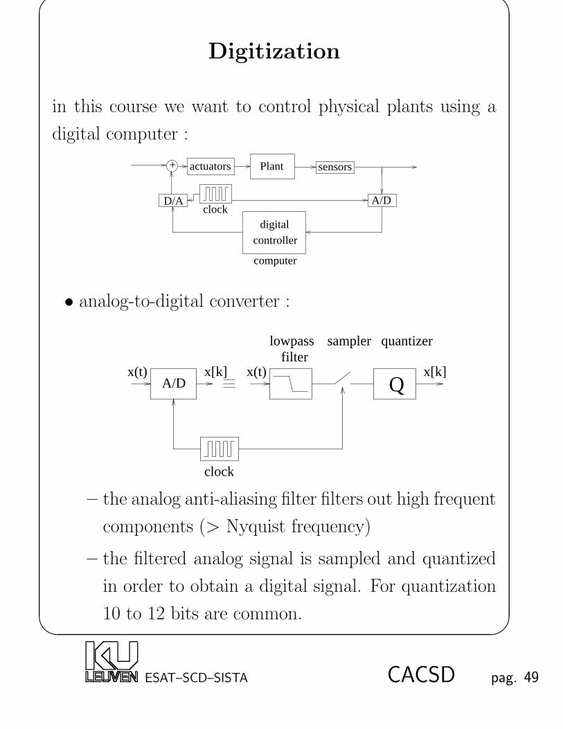
Digitization

in this course we want to control physical plants using a

digital computer :

Plant

A/D

controllerdigital

sensors

clock

actuators+

D/A

computer

• analog-to-digital converter :

clock

A/Dx(t) x[k] x(t)

filterlowpass sampler quantizer

Qx[k]

– the analog anti-aliasing filter filters out high frequent

components (> Nyquist frequency)

– the filtered analog signal is sampled and quantized

in order to obtain a digital signal. For quantization

10 to 12 bits are common.


'

&

$

%

• digital-to-analog converter :

– zero-order hold

0 10 20 30 40 50 60 70 80 90 100−4

−3

−2

−1

0

1

2

3

time

ZOH approximation

∗ introduces a delay

∗ frequency spectrum deformation

– first-order hold

– n-th order polynomial (more general case) : fit a n-

th order polynomial through the n+1 most recent

samples and extrapolate to the next time instance


'

&

$

%

Digitization of state space models1. discretization by applying numerical integration rules :

a continuous-time integrator

x(t) = e(t)

⇔sX(s) = E(s)

can be approximated using

• the forward rectangular rule or Euler’s method

xk+1 − xkTs

= ek

⇔z − 1

TsX(z) = E(z)

with xk = x(kTs)

t

e(t)

k-1 k k+1

• the backward rectangular rule

xk+1 − xkTs

= ek+1

⇔z − 1

zTsX(z) = E(z)

t

e(t)

k-1 k k+1


'

&

$

%

• the trapezoid rule or bilinear transformation

xk+1 − xkTs

=ek+1 + ek

2

⇔2

Ts

z − 1

z + 1X(z) = E(z)

t

e(t)

k-1 k k+1

Change a continuous model G(s) into a discrete model

Gd(z) by replacing all integrators with their discrete equiv-

alents := projection of the left half-plane

Euler backward rect. bilinear transf.

s→ z−1Ts

s→ z−1zTs

s→ 2Tsz−1z+1

Re

Im

Re

Im

Re

Im

Except for the forward rectangular rule stable continuous

poles (grey zone) are guaranteed to be placed in stable

discrete areas, i.e. within the unit circle.

The bilinear transformation maps stable poles → stable

poles and unstable poles → unstable poles.


'

&

$

%

The following continuous-time model is given :

x = Ax +Bu

y = Cx +Du⇔

sX = AX +BU

Y = CX +DU

following Euler’s method s is replaced by z−1Ts

, so

z − 1

TsX = AX +BU

or

zX = (I + ATs)X + BTsU

the output equation Y = CX + DU remains. A similar

calculation can be done for the backward rectangular rule

and the bilinear transformation resulting in the following

table :

Euler backward rect. bilinear transf.

Ad I + ATs (I −ATs)−1 (I − ATs2

)−1(I + ATs2

)

Bd BTs (I −ATs)−1BTs (I − ATs2 )−1BTs

Cd C C(I − ATs)−1 C(I − ATs2

)−1

Dd D D + C(I −ATs)−1BTs D + C(I − ATs2 )−1BTs

2


'

&

$

%

2. discretization by assuming zero-order hold ...

x = Ax +Bu

⇒x(t) = eAtx(0) +

∫ t

0

eA(t−τ)Bu(τ )dτ︸︷︷︸

convolution integral

Let the sampling time be Ts, then

x(t + Ts) = eA(t+Ts)x(0) +

∫ t+Ts

0

eA(t+Ts−τ)Bu(τ )dτ

= eATsx(t) + eATs∫ t+Ts

t

eA(t−τ)Bu(τ )dτ︸︷︷︸

approximated

ZOH⇒ xk+1t=kTs= eATsxk + eATsA−1(I − e−ATs)Buk= eATs︸︷︷︸

Ad

xk + A−1(eATs − I)B︸︷︷︸

Bd

uk

One can prove that Gd(z) can be expressed as

Gd(z)ZOH= (1− z−1)Z

L−1

G(s)

s

For this reason this discretization method is sometimes

called step invariance mapping.


'

&

$

%

3. discretization by zero-pole mapping :

following the previous method the poles of Gd(z) are

related to the poles of G(s) according to z = esTs. If

we assume by simplicity that also the zeros undergo this

transformation, the following heuristic may be applied:

(a) map poles and zeros according to z = esTs

(b) if the numerator is of lower order than the denomi-

nator, add discrete zeros at -1 until the order of the

numerator is one less than the order of the denomi-

nator. A lower numerator order corresponds to zeros

at∞ in continuous time. By discretization they are

put at -1.

(c) adjust the DC gain such that

lims→0

G(s) = limz→1

Gd(z)


'

&

$

%

Example :

given the following SISO system

[

A B

C D

]

=

−0.2 −0.5 1

1 0 0

1 0.4 0

⇒ G(s) = C(sI − A)−1B +D =s + 0.4

s2 + 0.2s + 0.5.

Now compare the following discretization methods (Ts = 1

sec.) :

1. bilinear transformation :

(a) Ad, Bd, Cd and Dd are calculated using the conver-

sion table

(b) Gbilinear(z) = Cd(zI − Ad)−1Bd +Dd.

=0.4898 + 0.1633z−1 − 0.3265z−2

1− 1.4286z−1 + 0.8367z−2

2. ZOH :

(a) Ad = eATs, Bd = A−1(eATs − I)B, Cd = C and

Dd = D

(b) GZOH(z) = Cd(zI − Ad)−1Bd +Dd.

=1.0125z−1 − 0.6648z−2

1− 1.3841z−1 + 0.8187z−2


'

&

$

%

3. pole-zero mapping :

(a) the poles of G(s) are −0.1 + j0.7 and −0.1− j0.7(b) there is one zero at −0.4(c)

Gpz = Kz − e−0.4

(z − e−0.1+j0.7)(z − e−0.1−j0.7)

= Kz−1 − 0.6703z−2

1− 1.3841z−1 + 0.8187z−2

hence K =lims→0G(s)

limz→1Gpz(z)= 1.0546

Compare the bode plots :

10−2

10−1

10−1

100

101

frequency (Hz)

freq

uenc

y am

plitu

de s

pect

rum

__ : continuous system

−− : bilinear approximation−. : zero−order hold assumption

.. : pole−zero mapping

10−2

10−1

−150

−100

−50

0

50

frequency (Hz)

phas

e sp

ectr

um (

degr

.)

__ : continuous system

−− : bilinear approximation−. : zero−order hold assumption.. : pole−zero mapping


'

&

$

%

Sampling rate selection :

• the lower the sampling rate, the lower the implementa-

tion cost (cheap microcontroller & A/D converters), the

rougher the response and the larger the delay between

command changes and system response.

• an absolute lower bound is set by the specification to

track a command input with a certain frequency :

fs ≥ 2BWcl

fs is the sampling rate and BWcl is the closed-loop sys-

tem bandwidth.

• if the controller is designed for disturbance rejection,

fs > 20BWcl

• when the sampling rate is too high, finite-word effects

show up in small word-size microcontrollers (< 10 bits).

• for systems where the controller adds damping to a

lightly damped mode with resonant frequency fr,

fs > 2fr

In practice, the sampling rate is a factor 20 to 40 higher

than BWcl.


'

&

$

%

Advantages of state space models

• More general models: LTI and Nonlinear Time Varying

(NTV).

• Geometric concepts: more mathematical tools (linear

algebra).

• Internal and external descriptions: “divide and con-

quer” strategy.

• Unified framework: the same for SISO and MIMO.


'

&

$

%

Geometric properties of linear statespace models

Canonical formsControl canonical form (SISO):

x = Acx + Bcu, y = Ccx.

Ac =

−a1 −a2 · · · · · · −an1 0 · · · · · · 0

0 . . . . . . ...... . . . . . . . . . ...

0 · · · 0 1 0

, Bc =

1

0...

0

,

Cc =[

b1 b2 · · · bn]

Corresponding transfer function:

G(s) =b(s)

a(s)

b(s) = b1sn−1 + b2s

n−2 + · · · + bn

a(s) = sn + a1sn−1 + a2s

n−2 + · · · + an


'

&

$

%

Block diagram for the control canonical form

x1 x2 xn−1

b1

b2

bn−1

bn

−a1

−a2

−an−1

−an

u

y

∫ ∫ ∫ ∫

xn


'

&

$

%

Modal canonical form:

x = Amx + Bmu, y = Cmx.

Am =

−s1

−s2

. . .

−sn

, Bm =

1

1...

1

Cm =[

r1 r2 · · · rn]

Corresponding transfer function:

G(s) =

n∑

i=1

ris + si

Block diagram for the modal canonical form:

yu

∫

∫

r1

rn

−s1

∫

−s2

−sn

r2

x1

x2

xn


'

&

$

%

Similarity transformationA state space model (A,B,C,D) is not unique for a phys-

ical system. Let

x = T x, det(T ) 6= 0,

A = T−1AT, B = T−1B, C = CT, D = D

⇒˙x = T−1ATx + T−1Bu = Ax + Bu,

y = CTx +Du = Cx +Du

T is chosen to give the most convenient state-space descrip-

tion for a given problem (e.g.control or modal canonical

forms).

Example: Eigenvalue decomposition of A:

A = XΛX−1, Λ =

α1 β1

−β1 α1

. . .

λ1

. . .

x = Ax +Bu

y = Cx +Du

X−1x = z=⇒ z = Λz +X−1Bu

y = CXz +Du


'

&

$

%

Controllability

An n-th order system is called controllable if one can reach

any state x from any given initial state x0 in a finite time.

Controllability matrix:

C =[

B AB · · · An−1B]

rank(C) = n⇔ (A,B) controllable

Explanation:

Consider a linear (discrete) system of the form

xk+1 = Axk +Buk

Then

xk+1 = Ak+1x0 + AkBu0 + · · · +Buk

such that

xk+1 − Ak+1x0 =[

B AB · · · AkB]

uk

uk−1

...

u0


'

&

$

%

Note that

rank[

B AB · · · AkB]

= rank[

B AB · · · An−1B]

for k ≥ n− 1 (Cayley-Hamilton Theorem).

There exists always a vector

uk

uk−1

...

u0

if rank(C) = n.

Remarks: Controllability matrices for a continuous time

system and a discrete time system are of the same form.


'

&

$

%

ObservabilityAn n-th order system is called observable if knowledge of

the input u and the output y over a finite time interval is

sufficient to determine the state x.

Observability matrix:

O =

C

CA...

CAn−1

rank(O) = n⇔ (A,C) observable

Explanation:

Consider an autonomous system

xk+1 = Axk

yk = Cxk

Then we find easily

yk = CAkx0


'

&

$

%

and

y0

y1

...

yk

=

C

CA...

CAk

x0

Note that

rank

C

CA

· · ·CAk

= rank

C

CA

· · ·CAn−1

for k ≥ n− 1.

One can always determine x0 if rank(O) = n.

Remarks: Observability matrices for a continuous time sys-

tem and a discrete time system are of the same form.


'

&

$

%

The Popov-Belevitch-Hautus tests (PBH)

PBH controllability test:

(A,B) is not controllable if and only if there exists a left

eigenvector q 6= 0 of A such that

ATq = qλ

BTq = 0

In other words, (A,B) is controllable if and only if there is

no left eigenvector q of A that is orthogonal to B.

If there is a λ and q satisfying the PBH test, then we

say that the mode corresponding to eigenvalue λ is uncon-

trollable (uncontrollable mode), otherwise it is controllable

(controllable mode).

How to understand (for SISO) ? Put A in the modal canon-

ical form:

A =

∗λi

∗

, B =

∗0

∗

,⇒ q =

0

1

0

Uncontrollable mode: xi = λixi.


'

&

$

%

PBH observability test:

(A,C) is not observable if and only if there exists a right

eigenvector p 6= 0 of A such that

Ap = pλ

Cp = 0

If there is a λ and p satisfy the PBH test, then we say that

the mode corresponding to eigenvalue λ is unobservable

(unobservable mode), otherwise it is observable (observable

mode).

How to understand for SISO ? Put A in a modal canonical

form.


'

&

$

%

Stability/Stabilizability/Detectability

Stability:

A system with system matrix A is unstable if A has an

eigenvalue λ with real(λ) ≥ 0 for a continuous time system

and |λ| ≥ 1 for a discrete time system.

Stabilizability:

(A,B) is stabilizable if all unstable modes are controllable.

Detectability:

(A,C) is detectable if all unstable modes are observable.


'

&

$

%

Example

xk+1 = Axk +Buk

yk = Cxk +Duk

[

A B

C D

]

=

1.1 0 0 0 1

0 −0.5 0.6 0 2

0 −0.6 −0.5 0 −1

0 0 0 2 2

0 1 2 3 1

Modes Stable? Stabilizable? Detectable?

1.1 no yes no

−0.5± 0.6i yes yes yes

2 no yes yes


'

&

$

%

Kalman decomposition and minimal realization

Kalman decomposition

Given a state space system [A,B,C,D]. Then we can

always find an invertible similarity transformation T such

that the transformed matrices have the structure

TAT−1 =

r1 r2 r3 r4

r1 Aco 0 A13 0

r2 A21 Aco A23 A24

r3 0 0 Aco 0

r4 0 0 A43 Aco

TB =

m

r1 Bco

r2 Bco

r3 0

r4 0

, CT−1 =(r1 r2 r3 r4

p Cco 0 Cco 0)

where

r1 = rank (OC), r2 = rank (C)− r1,r3 = rank (O)− r1, r4 = n− r1 − r2 − r3.


'

&

$

%

The subsystem

[ Aco, Bco, Cco, D ]

is controllable and observable. The subsystem

[

(

Aco 0

A21 Aco

)

,

(

Bco

Bco

)

,(

Cco 0)

, D ]

is controllable. The subsystem

[

(

Aco A13

0 Aco

)

,

(

Bco

0

)

, ( Cco Cco ), D ]

is observable. The subsystem

[ Aco , 0, 0, D ]

is neither controllable nor observable.


'

&

$

%

Kalman decomposition

u yCO

CO

CO

CO


'

&

$

%

Minimal realization:

A minimal realization is one that has the smallest-size A

matrix for all triplets [A,B,C] satisfying

G(s) = D + C(sI − A)−1B

where G(s) is a given transfer matrix.

[

A B C D]

is minimal ⇔ controllable and observable.

Let[

Ai Bi Ci D]

, i = 1, 2, be two minimal realizations

of a transfer matrix, then[

A1 B1 C1 D]

T ⇓ ⇑ T−1

[

A2 B2 C2 D]

with

T = C1CT2 (C2CT2 )−1


'

&

$

%

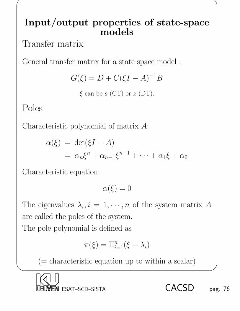
Input/output properties of state-spacemodels

Transfer matrix

General transfer matrix for a state space model :

G(ξ) = D + C(ξI − A)−1B

ξ can be s (CT) or z (DT).

Poles

Characteristic polynomial of matrix A:

α(ξ) = det(ξI − A)

= αnξn + αn−1ξ

n−1 + · · · + α1ξ + α0

Characteristic equation:

α(ξ) = 0

The eigenvalues λi, i = 1, · · · , n of the system matrix A

are called the poles of the system.

The pole polynomial is defined as

π(ξ) = Πni=1(ξ − λi)

(= characteristic equation up to within a scalar)


'

&

$

%

Physical interpretation of a pole :Consider the following second order system :

[

A B

C D

]

=

α β b1

−β α b2

c1 c2 0

The transfer matrix is given by (try to verify it) :

G(ξ) = C(ξI − A)−1B +D

=ξ(b1c1 + b2c2) + β(b2c1 − b1c2)− α(b1c1 + b2c2)

ξ2 − 2αξ + α2 + β2

There are 2 poles at α± jβ.

There is a zero at

α(b1c1 + b2c2)− β(b2c1 − b1c2)b1c1 + b2c2


'

&

$

%

In continuous time the impulse response takes on the form:

g(t) = L−1 G(s)

= L−1

s(b1c1 + b2c2) + β(b2c1 − b1c2)− α(b1c1 + b2c2)

s2 − 2αs + α2 + β2

= (Am cos(βt) +Bm sin(βt))eαt = Cmeαt cos(βt + γ)

with Am = b1c1 + b2c2 and Bm = b2c1 − b1c2

⇒ Cm =√

(b21 + b22)(c21 + c22)

⇒ γ = atan

(−Bm

Am

)

Define the damping ratio ζ and natural frequency ωn:

α = −ζωn, β = ωn√

1− ζ2

jω

θ

α + jβ

α− jβ

β

α

ζ = sin θωn

stability degree

r


'

&

$

%

For a second order system

G(s) =ω2n

s2 + 2ζωns + ω2n

the time response looks like :

rise time tr ' 1.8ωn

settling time ts = 4.6ζωn

peak time tp = πωd

, ωd = ωn√

1− ζ2

overshoot Mp = e−πζ/√

1−ζ2, 0 ≤ ζ < 1

In general : if a continuous-time system (A,B,C, 0) has

poles at α ± jβ ⇒ the impulse response will have time

modes of the form

Ameαt cos(βt + γ)

Am: amplitude

γ: phase

determined by B and C.


'

&

$

%

In discrete time the impulse response matrix Gd(k) takes

on the form :

Gd(k) = CdAk−1d Bd, k ≥ 1

which can be proven to be a sum of terms of the form :

Cmbk−1 cos(ω(k − 1) + γ)

each of which satisfies a second order linear system

[

A B

C D

]

=

α β b1

−β α b2

c1 c2 0

Parameterize A as

A =

[

b cosω b sinω

−b sinω b cosω

]

then

Ak = bk

[

cosωk sinωk

− sinωk cosωk

]


'

&

$

%

Now,

CAkB = (Am cosωk +Bm sinωk)bk

= Cmbk cos(ωk + γ)

with Am = Cm cos γ = b1c1 + b2c2

and Bm = −Cm sin γ = b2c1 − b1c2

⇒ Cm =√

(b21 + b22)(c21 + c22)

⇒ b =√

α2 + β2

⇒ ω = atan

(β

α

)

⇒ γ = atan

(−Bm

Am

)


'

&

$

%

Transmission zeros

Definition: The zeros of a LTI system are defined as those

values ζ ∈ C for which the rank of the transfer matrixG(ξ)

is lower than its normal rank (=rank of G(ξ) for almost all

values of ξ):

rank(G(ζ)) < normal rank

Property: Let ζ be a zero of G(ξ) (p×m), then

rank (G(ζ)) < normal rank,

⇓ if ζ is not a pole of G(ξ)

∃v 6= 0 s.t.[D + C(ζI − A)−1B

]v = 0,

⇓ define w∆= (ζI − A)−1Bv

Dv + Cw = 0, (ζI − A)w −Bv = 0,

⇓[

ζI − A −BC D

][

w

v

]

= 0


'

&

$

%

How to find zeros for square MIMO systems (p = m) with

invertible D ?

(ζI − A)w −Bv = 0, Cw +Dv = 0

⇓Aw +Bv = wζ, v = −D−1Cw

⇓(A−BD−1C)w = wζ

ζ = eigenvalue of A− BD−1C,

w = corresponding eigenvector !

For other cases :

• Generalized eigenvalue problem.

• Use Matlab function “tzero”.

Minimum and non-minimum phase systems:

If a system has an unstable zero (in the right half–plane

(RHP) or outside the unit circle), then it is a non-minimum

phase (NMP) system, otherwise it is a minimum phase

(MP) system.


'

&

$

%

Physical explanation (continuous time) :

Let ζ be a real zero, then there will exist vectors x0 and u0

such that: [

ζI − A −BC D

][

x0

u0

]

= 0

This means if we have an input u0eζt, there exists an initial

state x0 such that the response is

y(t) = 0.

For complex zeros :

if ζ is a complex zero, then also its complex conjugate ζ∗

is a zero. Try to prove that if[

ζI − A −BC D

][

x0

u0

]

= 0

the output y(t) will be exactly zero if the input is

u(t) = |u0|eReζt · cos(Imζt + φu0)

and the initial state is chosen to be Rex0. “·” is the

elementwise multiplication, both “cos()” and “e()” are as-

sumed to be elementwise operators,Rex0 is the real part

of x0, Imζ is the imaginary part of ζ and u0 = |u0|·ejφu0.Try to derive equivalent formulas for the discrete-time case.


'

&

$

%

Why zeros are important :

• Limited control system performance

k

C G

If G is NMP, k can not go to ∞, since unstable zeros

(which become unstable poles) put a limit on high gains.

• Stability of a stabilizing controller, Parity Interlacing

Property (PIP) :

Let G be unstable. Then, G can be stabilized by a

controller C which itself is stable⇔ between every pair

of real RHP zeros of G (including at ∞), there is an

even number of poles.

Example:

G(s) =s

s2 − 1

× ×−1 10

pole zero pole

∞

zero

-∞

G(s) can not be stabilized by a stable controller.


'

&

$

%

RHP zeros can cause undershoot !

Let

G(s) =Πni=1(1− s

ζi)

Πn+ri=1 (1− s

λi),

where r = relative degree of G(s). Let y(t) be the step

response.

Fact :

y(0) and its first r − 1 derivative are 0;

y(r) is the first non-zero derivative;

y(∞) = G(0).

The system has undershoot ⇔ the steady state value

y(∞) has a sign opposite to y(r)(0), i.e.

y(r)(0)y(∞) < 0.

It can be proven that the system has undershoot ⇔ there

is an odd number of RHP zeros.


'

&

$

%

An example of state-space analysis

Example: Tape drive control - state space analysis

Controllability/observability

Direct rank test using SVD:

The singular values of C are

4.5762, 4.3861, 1.2940, 1.2758, 0.5737, 0.4787,

so the system is controllable (rank=6).

The singular values of O are

2.5695, 1.4504, 0.7145, 0.7071, 0.5171, 0.2356,

so the system is observable (rank=6).


'

&

$

%

PBH test:

There are 6 (independent) left eigenvectors associated with

the 6 eigenvalues of A :

−0.1480± 0.0826i

0.0703± 0.5380i

0.1480∓ 0.0826i

−0.0703∓ 0.5380i

0.2994± 0.2954i

−0.2994∓ 0.2954i

,

0.0766

0.5624

0.0766

0.5624

0.4218

0.4218

0

0.4892

0.0000

0.4892

0.5105

0.5105

,

−0.0046

−0.0227

0.0046

0.0227

−0.7067

0.7067

,

0.0000

−0.0295

0.0000

−0.0295

−0.7065

−0.7065

It can be easily checked that none of them is orthogonal to

B. The result is the same as the rank test above.

The same can be done to investigate the observability.


'

&

$

%

Poles and zeros:

Poles: the eigenvalues of A are

−0.2370± 0.5947i, 0, −0.2813, −0.9760, −0.9687

The system is not stable since there is a pole at zero.

The first two oscillatory poles are from the spring-mass

system consisting of the tape and the motor/capstan in-

ertias. The zero pole reflects the pure integrative effect of

the tape on the capstans.


'

&

$

%

Zeros: it can be checked in Matlab using function “tzero”

that there is only one zero at -2. The eigenvector of the

matrix [

−2I − A −BC 0

]

associated with the eigenvalue 0 is

[

x0

u0

]

with x0 =

−0.1959

0.1959

0.1959

−0.1959

−0.4571

0.4571

, u0 =

[

0.4630

−0.4630

]

.

Thus, let

x(0) = x0, u(t) = u0e−2t,

then the output y(t) will be always zero, ∀t ≥ 0.


'

&

$

%

Physical explanation of the zero:

Since the initial values i1(0) = −i2(0) and the inputs

e1(t) = −e2(t), and the motor drive systems in both sides

are symmetric, the two capstans will rotate at the same

speed, but in opposite directions. So the tape position over

the read/write head will remain at 0 if the initial value is

at 0.

The tension in the tape is the sum of the tensions in the

tape spring and the tape damping. The input voltages vary

such a way that the tensions in the tape spring and the tape

damping cancel each other out.


'

&

$

%

Matlab Functions

c2d

c2dm

canon

expm

tf2ss

ss2tf

(d)impulse

(d)step

minreal

tzero

ctrb

obsv

ctrbf

obsvf

(d)lsim

ss

ssdata


'

&

$

%

Chapter 3

State Feedback - Pole Placement

Motivation

Whereas classical control theory is based on output feed-

back, this course mainly deals with control system design

by state feedback. This model-based control strategy con-

sists of

Step 1. State feedback control-law design.

Step 2. Estimator design to estimate the state vector.

Step 3. Compensation design by combining the control

law and the estimator.

Step 4. Reference input design to determine the zeros.


'

&

$

%

Schematic diagram of a state-space design

example

ux = Ax+Bu

x

C

r˙x = Ax+Bu

+L(y − r − Cx)estimatorcontrol-law

−K

plant

compensator

x y

−


'

&

$

%

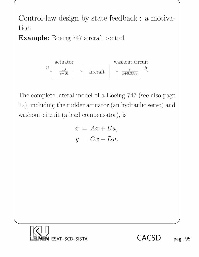
Control-law design by state feedback : a motiva-tionExample: Boeing 747 aircraft control

10s+10

ss+0.3333aircraft

washout circuitactuatoru y

The complete lateral model of a Boeing 747 (see also page

22), including the rudder actuator (an hydraulic servo) and

washout circuit (a lead compensator), is

x = Ax +Bu,

y = Cx +Du.


'

&

$

%

where

A =

−10 0 0 0 0 0

0.0729 −0.0558 −0.997 0.0802 0.0415 0

−4.75 0.598 −0.115 −0.0318 0 0

1.53 −3.05 0.388 −0.465 0 0

0 0 0.0805 1 0 0

0 0 1 0 0 −0.3333

B =

1

0

0

0

0

0

, C =[

0 0 1 0 0 −0.3333]

, D = 0.

The system poles are

−0.0329± 0.9467i, −0.5627, −0.0073, −0.3333, −10.


'

&

$

%

The poles at −0.0329 ± 0.9467i have a damping ratio

ζ = 0.03 which is far from the desired value ζ = 0.5. The

following figure illustrates the consequences of this small

damping ratio.

Initial condition response with β = 1.

0 50 100 150−0.01

−0.005

0

0.005

0.01

0.015

Time (secs)

Am

plitu

de

To improve this behavior, we want to design a control law

such that the closed loop system has a pair of poles with a

damping ratio close to 0.5.


'

&

$

%

General Format of State Feedback

Control law

u = −Kx, K : constant matrix.

For single input systems (SI):

K =[

K1 K2 · · · Kn

]

For multi input systems (MI):

K =

K11 K12 · · · K1n

K21 K22 · · · K2n

... ... . . . ...

Kp1 Kp2 · · · Kpn

Note: one sensor is needed for each state ⇒ disadvantage.

We’ll see later how to deal with this problem (estimator

design).


'

&

$

%

Structure of state feedback control

uC

Plant

x yx = Ax+Bu

u = −Kx

Control-law


'

&

$

%

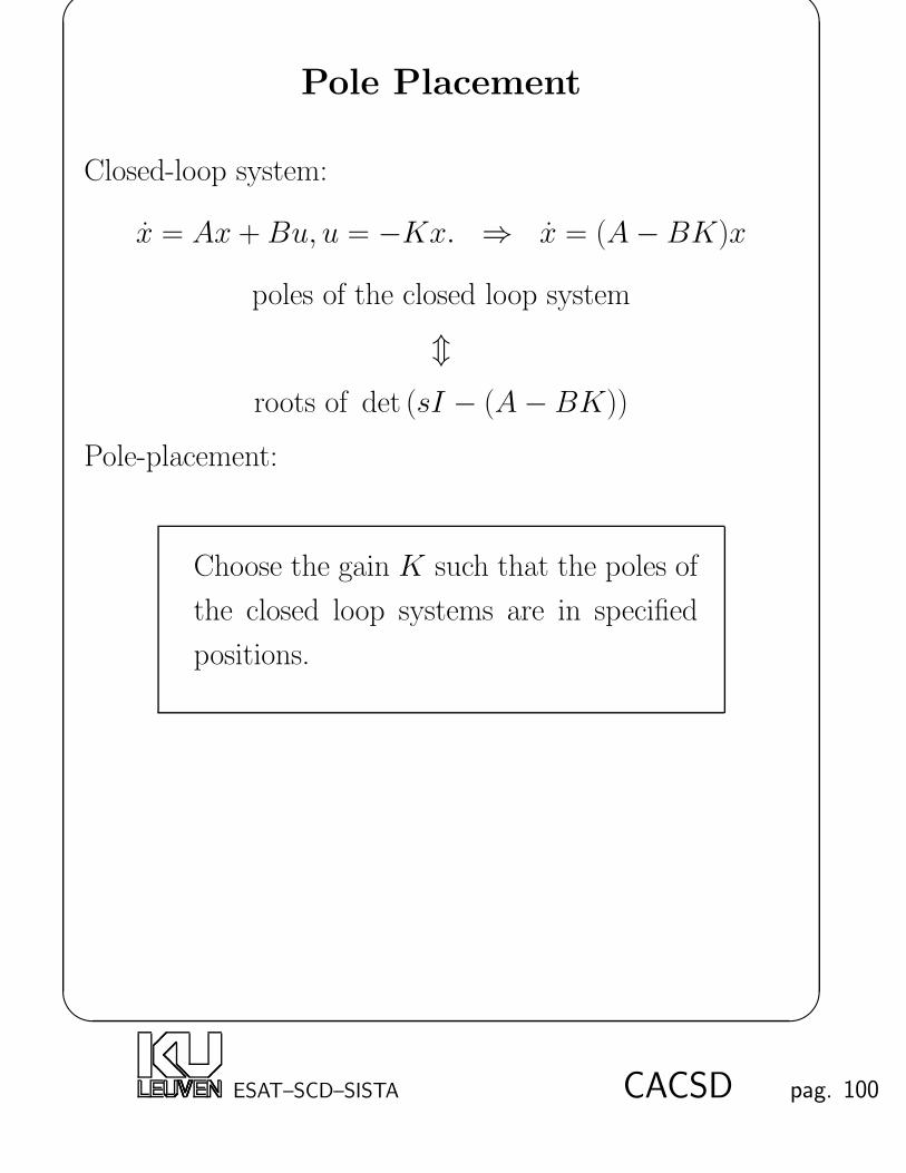
Pole Placement

Closed-loop system:

x = Ax +Bu, u = −Kx. ⇒ x = (A−BK)x

poles of the closed loop system

mroots of det (sI − (A−BK))

Pole-placement:

Choose the gain K such that the poles of

the closed loop systems are in specified

positions.


'

&

$

%

More precisely, suppose that the desired locations are given

by

s = s1, s2, · · · , snwhere si, i = 1, · · · , n are either real or complex conjugated

pairs, choose K such that the characteristic equation

αc(s)∆= det (sI − (A− BK))

equals

(s− s1)(s− s2) . . . (s− sn).


'

&

$

%

Pole-placement - direct methodFind K by directly solving

det (sI − (A− BK)) = (s− s1)(s− s2) · · · (s− sn)

and matching coefficients in both sides.

Disadvantage:

• Solve nonlinear algebraic equations, difficult for n>3.

Example Let n = 3, m = 1. Then the following

3rd order equations have to be solved to find K =[

K1 K2 K3

]

:

∑

1≤i≤3

(aii − biKi) =∑

1≤i≤3

si,

∑

1≤i<j≤3

∣∣∣∣∣

aii − biKi aij − biKj

aji − bjKi ajj − bjKj

∣∣∣∣∣

=∑

1≤i<j≤3

sisj,

∣∣∣∣∣∣∣

a11 − b1K1 a12 − b1K2 a13 − b1K3

a21 − b2K1 a22 − b2K2 a23 − b2K3

a31 − b3K1 a32 − b3K2 a33 − b3K3

∣∣∣∣∣∣∣

= s1s2s3.

• You never know whether there IS a solution K. (But

THERE IS one if (A,B) is controllable!)


'

&

$

%

Pole-placement for SI: Ackermann’s methodLet Ac, Bc be in a control canonical form, then

Ac−BcKc =

−a1 −K1 −a2 −K2 · · · · · · −an −Kn

1 0 · · · · · · 0

0 . . . . . . ...... . . . . . . . . . ...

0 · · · 0 1 0

and

det (sI − (Ac − BcKc)) =

sn + (a1 +K1)sn−1 + (a2 +K2)s

n−2 + · · · + (an +Kn)

If

(s−s1)(s−s2) · · · (s−sn) = sn+α1sn−1+α2s

n−2+· · ·+αnthen

K1 = −a1 + α1, K2 = −a2 + α2, · · · , Kn = −an + αn.


'

&

$

%

Design procedure (when A,B are not in control canonical

form):

• Transform (A,B) to a control canonical form (Ac, Bc)

with a similarity transformation T .

• Find control law Kc with the procedure on the previous

page.

• Transform Kc: K = KcT−1.

Note that the system (A,B) must be controllable.

Property:

For SI systems, control law K is unique!


'

&

$

%

The design procedure can be expressed in a more compact

form :

K =[

0 · · · 0 1]

C−1αc(A),

where C is the controllability matrix:

C =[

B AB · · · An−1B]

and

αc(A) = An + α1An−1 + α2A

n−2 + · · · + αnI.


'

&

$

%

Pole-placement for MI - SI generalization

Fact: If (A,B) is controllable, then for almost any Kr ∈Rm×n and almost any v ∈ R

m, (A−BKr, Bv) is control-

lable.

⇓From the pole placement results for SI, there is a Ks ∈R1×n so that the eigenvalues of A − BKr − (Bv)Ks can

be assigned to desired values.

⇓

Also the eigenvalues of A−BK can be assigned to desired

values by choosing a state feedback in the form of

u = −Kx = −(Kr + vKs)x.


'

&

$

%

Design procedure:

• Arbitrarily choose Kr and v such that

(A−BKr, Bv) is controllable.

• Use Ackermann’s formula to find Ks for

(A−BKr, Bv).

• Find state feedback gain K = Kr + vKs.


'

&

$

%

Pole-placement for MIMO - Sylvester equation

Let Λ be a real matrix such that the desired closed-loop

system poles are the eigenvalues of Λ. A typical choice of

such a matrix is:

Λ =

α1 β1

−β1 α1

. . .

λ1

. . .

,

which has eigenvalues: α1± jβ1, . . . , λ1, . . . . which are the

desired poles of the closed-loop system. For controllable

systems (A,B) with static state feedback,

A−BK ∼ Λ.

⇒ There exists a similarity transformation X such that:

X−1(A−BK)X = Λ,

or

AX −XΛ = BKX.


'

&

$

%

The trick to solve this equation: split up the equation by

introducing an arbitrary auxiliary matrix G:

AX −XΛ = BG, (Sylvester equation in X)

KX = G.

The Sylvester equation is a matrix equation that is linear

in X . If X is solved for a known G, then

K = GX−1.

Design procedure:

• Pick an arbitrary matrix G.

• Solve the Sylvester equation for X .

• Obtain the static feedback gain K = GX−1.


'

&

$

%

Properties:

• There is always a solution for X if A and Λ have no

common eigenvalues.

• For SI, K is unique, hence independent of the choice of

G.

• For certain special choices of G this method may fail

(e.g.X not invertible or ill conditioned). Then just try

another G.


'

&

$

%

Examples for pole placement

Example Boeing 747 aircraft control - control law design

with pole placement (Ackermann’s method)

Desired poles:

−0.0051, −0.468, −1.106, −9.89, −0.279± 0.628i

which have a maximum damping ratio 0.4.

From the desired poles

αc(s) = s6 + 12.03s5 + 23.01s4 + 19.62s3 + 10.55s2 + 2.471s+ 0.0123,

αc(A) =

8844.70 0 0 0 0 0

368.20 7.88 2.43 −0.61 −0.16 0

4220.20 −2.47 5.93 −0.46 −0.23 0

−1459.94 −2.75 −25.73 2.78 1.09 0

115.27 25.80 −6.71 −0.82 0.08 0

−436.60 −5.95 0.06 0.28 0.06 0.13

is obtained and hence the controllability matrix is given by

C =

1.00 −10.00 100.00 −1000.00 10000.00 −100000

0 0.07 4.12 −42.22 418.15 −4180.52

0 −4.75 48.04 −477.48 4774.34 −47746.07

0 1.53 −18.08 167.47 −1664.37 16651.01

0 0 1.15 −14.21 129.03 −1280.03

0 0 −4.75 49.62 −494.03 4939.01

.


'

&

$

%

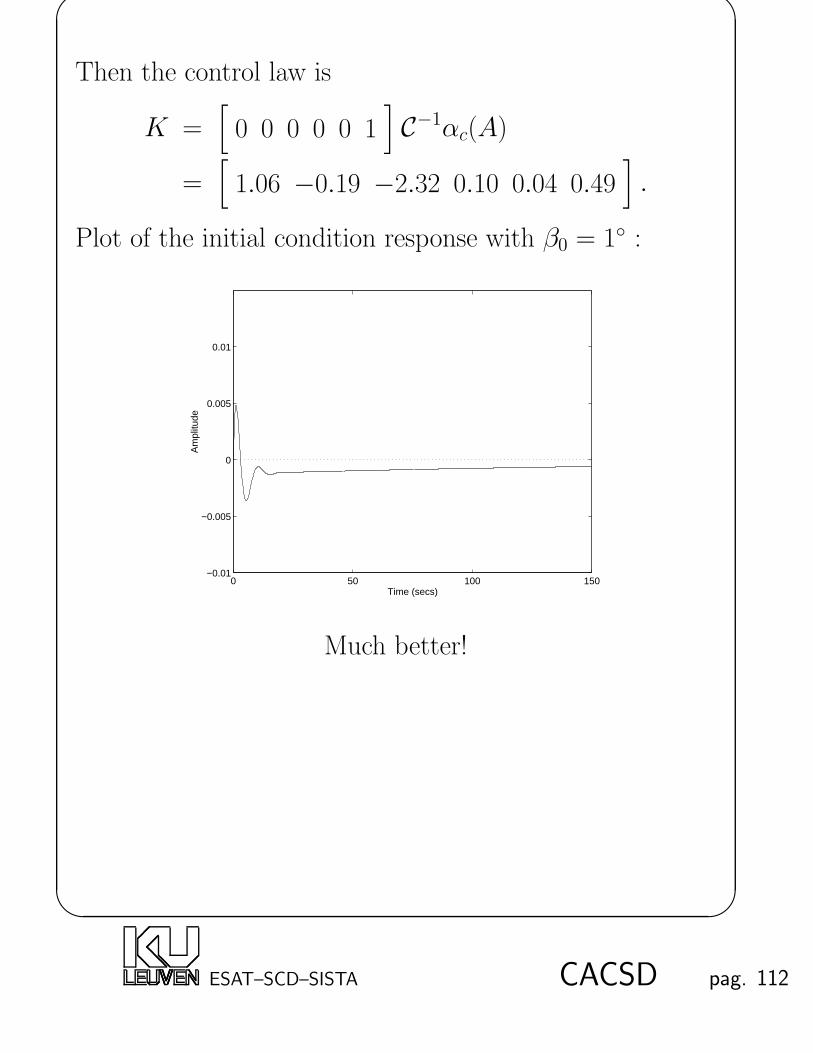
Then the control law is

K =[

0 0 0 0 0 1]

C−1αc(A)

=[

1.06 −0.19 −2.32 0.10 0.04 0.49]

.

Plot of the initial condition response with β0 = 1 :

0 50 100 150−0.01

−0.005

0

0.005

0.01

Time (secs)

Am

plitu

de

Much better!


'

&

$

%

Example Tape drive control - control law design with

pole placement (Sylvester equations)

Desired poles:

−0.451± 0.937i, −0.947± 0.581i, −1.16, −1.16.

Take an arbitrary matrix G:

G =

[

1.17 0.08 −0.70 0.06 0.26 −1.45

0.63 0.35 1.70 1.80 0.87 −0.70

]

.

Solve the Sylvester equation for X :

AX −XΛc = BG,

where

Λc =

−0.451 0.937

−0.937 −0.451

−0.947 0.581

−0.581 −0.947

−1.16

−1.16

.


'

&

$

%

X =

−0.27 −1.83 1.00 0.86 2.31 −10.78

0.92 0.29 −0.23 −0.70 −1.34 6.25

0.56 −0.76 −2.26 −6.25 6.42 −5.74

0.23 0.43 −0.75 3.62 −3.72 3.33

−0.62 0.91 0.17 1.19 1.40 −7.87

−0.58 0.33 2.99 −3.15 4.75 −3.76

.

Obtain the static feedback gain K = GX−1:

K =

[

0.55 1.58 0.32 0.56 0.67 0.05

0.60 0.60 0.68 3.24 −0.21 1.74

]

.

The closed loop system looks like :

x = Ax+ Bu

Process

−K

yuC

x

w


'

&

$

%

Impulse response (to w):

0 5 10 15 20−1

0

1

2

3Input1/Output1

0 5 10 15 20−0.3

−0.2

−0.1

0

0.1Input1/Output2

0 5 10 15 20−1

0

1

2

3Input2/Output1

0 5 10 15 20−0.1

0

0.1

0.2

0.3Input2/Output2

Dashed line: without feedback, sensitive to process noise.

Solid line: with state feedback, much better!


'

&

$

%

Property:Static state feedback does not change the transmission ze-

ros of a system:

zeros(A,B,C,D) = zeros(A−BK,B,C −DK,D)

Proof :

If ζ is a zero of (A,B,C,D), then (when ζ is not a pole),

there are u and v such that[

A B

C D

][

u

v

]

=

[

I 0

0 0

][

u

v

]

ζ

Now let u = u, v = Ku + v, then[

A− BK B

C −DK D

][

u

v

]

=

[

I 0

0 0

][

u

v

]

ζ

⇒ ζ is a zero of (A−BK,B,C −DK,D).


'

&

$

%

Pole location selection

Dominant second-order poles selectionUse the relations between the time specifications (rise time,

overshoot and settling time) and the second-order transfer

function with complex poles at radius ωn and damping

ratio ζ .

1. Choose the closed-loop poles for a high-order

system as a desired pair of dominant second-

order poles.

2. Select the rest of the poles to have real parts

corresponding to sufficiently damped modes,

so that the system will mimic a second-order

response with reasonable control effort.

3. Make sure that the zeros are far enough into

the left half-plane to avoid having any appre-

ciable effect on the second-order behavior.


'

&

$

%

Prototype designAn alternative for higher-order systems is to select proto-

type responses with desirable dynamics.

• ITAE transfer function poles : a prototype set of tran-

sient responses obtained by minimizing a certain crite-

rion of the form

J =

∫ ∞

0

t|e|dt.

Property: fast but with overshoot.

• Bessel transfer function poles : a prototype set of trans-

fer functions of 1/Bn(s) where Bn(s) is the nth-degree

Bessel polynomial.

Property: slow without overshoot.


'

&

$

%

Prototype Response Poles:

k Pole Location

(a) ITAE 1 −1

T.F. poles 2 −0.7071± 0.7071j

3 −0.7081, −0.5210± 1.068j

4 −0.4240± 1.2630j, 0.6260± 0.4141j

(b) Bessel 1 −1

T.F. poles 2 −0.8660± 0.5000j

3 −0.9420,−0.7455± 0.7112j

4 −0.6573± 0.8302j, −0.9047± 0.2711j

0 1 2 3 4 5 6 7 80

0.2

0.4

0.6

0.8

1

1.2Step responses for the ITAE prototypes

k=1

2

34

56

0 1 2 3 4 5 6 7 80

0.2

0.4

0.6

0.8

1

1.2Step responses for the Bessel prototypes

k=1

2

3

45

6

time (seconds) time (seconds)

Pole locations should be adjusted for faster/slower re-

sponse. A time scaling with factor α can be applied by

replacing the Laplace variable s in the transfer function by

s/α.


'

&

$

%

ExamplesExample Tape drive control - Selection of poles. The

poles selection methods above are basically for SI systems.

Thus consider only the one-motor (the left one) of the tape

drive system and set the inertia J of the right wheel 3 times

larger than the left one. Then

x = Ax +Bu,

y = Cx +Du,

where

x =

p1

ω1

p2

ω2

i1

, A =

0 2 0 0 0

−0.1 −0.35 0.1 0.1 0.75

0 0 0 2 0

0.1 0.1 −0.1 −0.35 0

0 −0.03 0 0 −1

,

B =[

0 0 0 0 1]T

, C =

[

0.5 0 0.5 0 0

−0.2 −0.2 0.2 0.2 0

]

,

D =

[

0

0

]

, y =

[

p3

T

]

, u = e1.


'

&

$

%

Specification: the position p3 has no more than 5% over-

shoot and a rise time of no more than 4 sec. Keep the

peak tension as low as possible.

Pole placement as a dominant second-order sys-tem:

Using the formulas on page 79, we find

Overshoot Mp < 5% ⇒ damping ratio ζ = 0.6901.

Rise time tr < 4 sec. ⇒ natural frequency ωn = 0.45

The formulas on page 79 are only approximative, therefore

we take some safety margin and choose for instance ζ = 0.7

and ωn = 1/1.5.

⇓Poles :

−0.707± 0.707j

1.5Other poles far to the left: −4/1.5, −4/1.5, −4/1.5. ⇒

K =[

8.5123 20.3457 −1.4911 −7.8821 6.1927]

.

Control law:

u = −Kx + 7.0212r,

where r is the reference input such that y follows r (in

steady state y = r).


'

&

$

%

Pole placement using an ITAE prototype:Check the step responses of the ITAE prototypes and ob-

serve that the rise time for the 5th order system is about

5 sec. So let α = 5/4 = 1.25. From the ITAE poles table,

the following poles are selected:

(−0.8955,−0.3764± 1.2920j,−0.5758± 0.5339j)× 1.25.

⇒ K =[

1.9563 4.3700 0.5866 0.8336 0.7499]

.

Control law:

u = −Kx + 2.5430r.

Pole placement using a Bessel prototype:Check the step responses of the Bessel prototypes, it ap-

pears that the rise time for the 5th order system is about

6 sec. So let α = 6/4 = 1.5. From the Bessel poles table,

the following poles are selected:

(−1.3896,−0.8859 ± 1.3608j,−1.2774 ± 0.6641j) × 1.5.

⇒ K =[

3.9492 9.1131 2.3792 5.2256 2.9662]

.

u = −Kx + 6.3284r.


'

&

$

%

Step responses:

0 1 2 3 4 5 6 7 8 9 100

0.2

0.4

0.6

0.8

1

1.2Step responses

Tap

e po

stio

n p3

Time: msec.

Bessel

ITAE

Dominant 2nd−order

0 1 2 3 4 5 6 7 8 9 10−0.2

−0.15

−0.1

−0.05

0

0.05Step responses

Tap

e te

nsio

n

Time: msec.

Dominant 2nd−order

ITAE

Bessel


'

&

$

%

Matlab Functions

poly

real

polyvalm

acker

lyap

place


'

&

$

%

Chapter 4

State Feedback – LQR

Motivation

Quadratic minimization : least squares

Consider the state space model

xk+1 = Axk +Buk,

yk = Cxk +Duk.

Find the control inputs uk, k = 0, . . . , N − 1 such that

JN =N−1∑

k=0

(wk − yk)T (wk − yk)

is minimized, where wk, k = 0, . . . , N − 1 is a given se-

quence. N is a predefined horizon.

The smaller JN , the closer the sequence yk is to the se-

quence wk.


'

&

$

%

The solution can be derived in terms of the following

input-output equations :

y0

y1

...

yN−1

︸︷︷︸

y

=

C

CA...

CAN−1

︸︷︷︸

ON

x0+

H0 0 · · · · · · 0

H1 H0 · · · · · · 0

H2 H1 H0 · · · 0

· · · · · · · · · · · · · · ·HN−1 HN−2 · · · · · · H0

︸︷︷︸

HN

u0

u1

...

uN−1

︸︷︷︸

u

where Hk are called the Markov parameters (impulse re-

sponse matrices) defined as :

H0 = D, Hk = CAk−1B, k = 1, 2, · · · , N − 1.

Let vector w be defined in a similar way as y, then

JN = wTw + xT0OTNONx0 + uTHT

NHNu

−2wTONx0 − 2wTHNu + 2xT0OTNHNu

is the quadratic criterion to be minimized.

Now find the optimal u as the solution to minu JN . In order

to do so we set the derivatives of JN with respect to the

vector u to zero, resulting in :

HTNHNu = HT

Nw −HTNONx0.


'

&

$

%

When HTNHN is invertible, then

uopt = (HTNHN)−1HT

N(w −ONx0),

which can be written as

u0

u1

...

uN−1

=

F0

F1

...

FN−1

x0+

G11 G12 · · · G1N

G21 G22 · · · G2N

· · · · · · · · · · · ·GN1 GN2 · · · GNN

w0

w1

...

wN−1

.

Constrained minimization : basics of MPC

The least squares solution can be complemented with lin-

ear constraints, for instance on the magnitude of the in-

put sequence or on its derivative. This then leads to a

quadratic programming problem (see Matlab quadprog.m).

One could require for instance that all components of the

input u are smaller in absolute value than a certain pre-

specified threshold or that they have to be nonnegative (to

avoid that too large or too small inputs are applied to the

actuators), that the first derivative of the input u stays

within certain bounds (to avoid abrupt changes in the in-

put), etc ... .


'

&

$

%

Example :

Consider the following SISO system

xk+1 =

0.7 0.5 0

−0.5 0.7 0

0 0 0.9

xk +

1

1

1

uk, x0 =

0.1

0.2

0.3

yk =[

0 −1 1]

xk + 0.5uk.

We want the output to be as close as possible to a prede-

fined w by minimizing (w−y)T (w−y), where w looks like

(N=20) :

0 2 4 6 8 10 12 14 16 18 20

−1

−0.8

−0.6

−0.4

−0.2

0

0.2

0.4

0.6

0.8

1

discrete time

ampl

itude

desired output w

Construct HN and ON . Now compute u as the least

squares solution to minu(w − y)T (w − y) (formula on top

of page 127).


'

&

$

%

The input u is shown in the figure below.

0 2 4 6 8 10 12 14 16 18 20−2500

−2000

−1500

−1000

−500

0

500

1000

discrete time

ampl

itude

least squares input u

It appears that if this input is applied to the system the

output is exactly the desired block wave we wanted.

The input however may be too large. Now let’s assume

that for safety reasons the input should stay between -100

and 100. Then we have to solve a constrained optimization

problem minimizing (w − y)T (w − y) with respect to u

and subject to −100 ≤ uk ≤ 100. This comes down to a

quadratic programming problem which basically solves

minu

1

2uTHu + fTu subject to Au ≤ b.

Matlab program quadprog.m can be used to solve this

equation.


'

&

$

%

H and f follow from the expression for JN on page 126 and

A and b depend on the constraints which are being applied.

The input is shown in the next figure

0 2 4 6 8 10 12 14 16 18 20

−100

−80

−60

−40

−20

0

20

40

60

80

100

discrete time

ampl

itude

constrained input u

and clearly remains between the predefined bounds. The

output follows the block wave quite well :

0 2 4 6 8 10 12 14 16 18 20

−1

−0.8

−0.6

−0.4

−0.2

0

0.2

0.4

0.6

0.8

1

discrete time

ampl

itude

output y and desired output w


'

&

$

%

A more general quadratic criterion is one in which the in-

puts and the outputs are weighted with two weighting ma-

trices R ∈ RmN×mN and Q ∈ R

pN×pN such that

JN = uTRu + (y − w)TQ(y − w).

In this way the controller can be better adjusted to the de-

signer’s wishes. Furthermore, it appears that this approach

is numerically more robust.

Try to express JN as a function of w, u, x0, ... as on page

126. The optimal solution is now given by

uopt = minuJN = (R+HT

NQHN)−1(HTNQw−HT

NQONx0).

Also in this case the minimization criterion can be comple-

mented with linear constraints.

The problem with the controller so far is that the input

sequences are not really generated by state feedback. If the

system model differs from the real system due to inaccurate

modeling or nonlinearities, the previous method might fail.

In practice therefore feedback is inserted. Further, only the

first element of vector uopt is applied to the system and uopt

is recomputed each sample instance. This basically leads to

the so–called Model–based Predictive Controller (MPC).


'

&

$

%

Linear Quadratic Regulator (LQR)

Solving a quadratic programming problem is a computa-

tionally intensive operation. For this purpose we propose

to use a simpler quadratic cost function of the form

N∑

k=0

(xTkQxk + uTkRuk)

where both Q and R are nonnegative definite. We also

constrain the optimization problem in this case, but now

requiring that uk = −Kxk. By introducing state feedback

the regulator is armed against model uncertainties, plant

changes, ... . Remark that using this simpler approach we

cannot force the input to stay within predefined bounds, as

with the MPC.

The central question is whether we can find a stabilizing

feedback matrix K in an easy way without having to solve

a complex optimization problem. In this chapter it will

become clear how to choose a feedback matrix K that is

optimal w.r.t. a quadratic criterion such as the one defined

on the previous page. This will lead to the Linear Quadratic

Regulator (LQR). Afterwards we’ll show how to design a

state estimator.


'

&

$

%

This overcomes that all state variables need to be mea-

sured. Measuring all state variables is too expensive or can

be even practically impossible. The chapter on reference

introduction and integral design shows how to extend the

feedback equation to uk = −Kxk + f(ref) such that track-

ing of an external signal is feasible.

First example of LQR :

Consider the system

xk+1 = xk + uk

and apply static feedback uk = −κxk. Suppose that the

cost function is given by∞∑

k=0

(x2k + ρu2

k).

If ρ is small, we don’t care about the magnitude of the

control inputs (cheap control) and we are mainly interested

in a fast response, requiring that the terms x2k are small.

If on the other hand ρ is large, we weigh the control input

heavily in the quadratic cost function (high cost).

We find easily that

xk = (1− κ)kx0


'

&

$

%

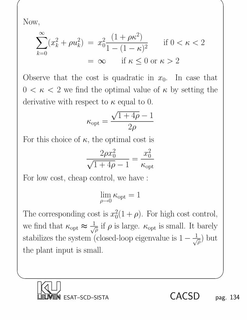
Now,∞∑

k=0

(x2k + ρu2

k) = x20

(1 + ρκ2)

1− (1− κ)2if 0 < κ < 2

= ∞ if κ ≤ 0 or κ > 2

Observe that the cost is quadratic in x0. In case that

0 < κ < 2 we find the optimal value of κ by setting the

derivative with respect to κ equal to 0.

κopt =

√1 + 4ρ− 1

2ρ

For this choice of κ, the optimal cost is

2ρx20√

1 + 4ρ− 1=

x20

κopt

For low cost, cheap control, we have :

limρ→0

κopt = 1

The corresponding cost is x20(1 + ρ). For high cost control,

we find that κopt ≈1√ρ

if ρ is large. κopt is small. It barely

stabilizes the system (closed-loop eigenvalue is 1− 1√ρ) but

the plant input is small.


'

&

$

%

LQRQuadratic minimization : state feedback

Given the linear time invariant discrete time system

xk+1 = Axk +Buk, x0 is known.

Find a control sequence uk, k = 0, . . . , N − 1 such that

JN =1

2

N−1∑

k=0

[xTkQxk + uTkRuk] +1

2xTNQNxN

is minimized. R, Q and QN are nonnegative definite

weighting matrices.


'

&

$

%

Lagrange multipliers method :

Take the state equations for k = 0, . . . , N − 1 as N con-

straints. There will be one Lagrange multiplier vector, lk+1,

for each value of k. Write the Lagrangean JN as

N−1∑

k=0

[1

2xTkQxk +

1

2uTkRuk + lTk+1(−xk+1 + Axk +Buk)

]

+1

2xTNQNxN .

Setting the derivatives with respect to uk, lk+1 and the xk

to zero results in a set of

control equations : uTkR + lTk+1B = 0,

state equations : −xk+1 + Axk +Buk = 0,

adjoint equations : xTkQ− lTk + lTk+1A = 0,

final state equations : QNxN − lN = 0.

⇒ Two-point boundary value problem.

The adjoint equations may also be written as

lk = AT lk+1 +Qxk

This equation runs backwards in time. In order to solve

this set of coupled difference equations we need to know

the initial condition on xk and the final condition on lk. x0

is assumed to be given.


'

&

$

%

Sweep method to solve the two-point boundaryvalue problem

Assume

lk = Skxk, for a certain matrix Sk.

The control equations become :

Ruk = −BTSk+1(Axk +Buk)

Solving for uk, we obtain

uk = −P−1k+1B

TSk+1Axk, with Pk+1 = R +BTSk+1B.

From the adjoint equations and the state equations :

Skxk = ATSk+1(Axk +Buk) +Qxk.

Combine these two equations :[Sk − AT

(Sk+1 − Sk+1BP

−1k+1B

TSk+1

)A−Q

]xk∀k= 0

⇒ Riccati difference equation :

Sk = AT[Sk+1 − Sk+1BP

−1k+1B

TSk+1

]A +Q.


'

&

$

%

This equation runs backwards in time. The boundary con-

dition on the recursion is obtained from the final state equa-

tions :

lN = QNxN = SNxN → SN = QN .

The final solution for finite horizon can be found by solving

for uk :

uk = −Kkxk,

where

Kk = (R + BTSk+1B)−1BTSk+1A.

This matrix Kk is the desired optimal time-varying feed-

back matrix. Note that the optimal gain sequence is in-

dependent of x0. It can be pre-computed if the system

matrices A and B are known and R, Q, QN and N are

specified.

The optimal cost is

JminN =

1

2xT0S0x0.


'

&

$

%

Example :

Consider the following discrete-time system

xk+1 = 0.3679xk + 0.6321uk, x0 = 1

Determine the control sequence that minimizes the follow-

ing cost function :

J =1

2

9∑

k=0

[x2k + u2

k] +1

2x2

10

Note that in this example Q = 1, R = 1 and QN = 1.

The Riccati difference equation we have to solve is

Sk = 0.3679[Sk+1− Sk+10.6321(1 + 0.6321Sk+10.6321)−10.6321Sk+1]0.3679 + 1

which can be simplified to

Sk = 1 + 0.1354Sk+1[1 + 0.3996Sk+1]−1

The boundary condition is SN = S10 = QN = 1.


'

&

$

%

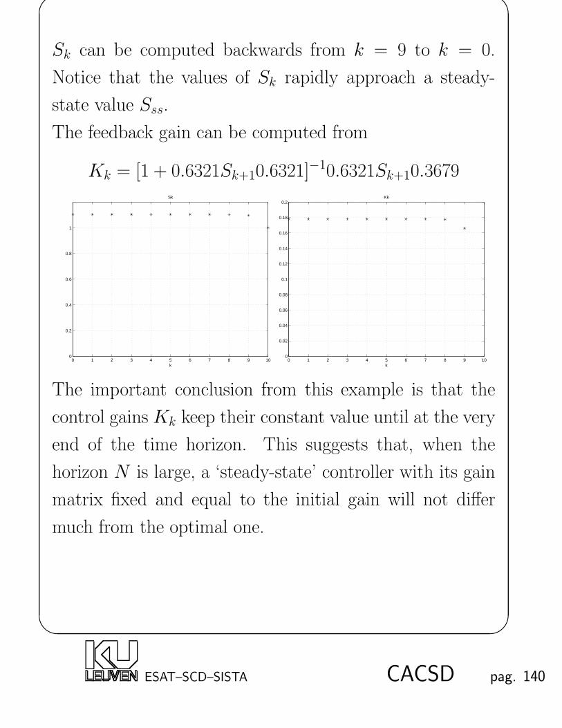
Sk can be computed backwards from k = 9 to k = 0.

Notice that the values of Sk rapidly approach a steady-

state value Sss.

The feedback gain can be computed from

Kk = [1 + 0.6321Sk+10.6321]−10.6321Sk+10.3679

0 1 2 3 4 5 6 7 8 9 100

0.2

0.4

0.6

0.8

1

k

Sk

0 1 2 3 4 5 6 7 8 9 100

0.02

0.04

0.06

0.08

0.1

0.12

0.14

0.16

0.18

0.2Kk

k

The important conclusion from this example is that the

control gains Kk keep their constant value until at the very

end of the time horizon. This suggests that, when the

horizon N is large, a ‘steady-state’ controller with its gain

matrix fixed and equal to the initial gain will not differ

much from the optimal one.


'

&

$

%

One can show that the set Sk converges to a steady-state

value S. S can be found from the so-called discrete alge-

braic Riccati equation :

S = AT[S − SB(R +BTSB)−1BTS

]A +Q.

The steady-state optimal control law is then time-invariant:

K = (R +BTSB)−1BTSA,

The feedback solution for infinite horizon is

uk = −Kxk.

The closed-loop system matrix A − BK is stable if the

system (A,B) is controllable and (A,R1/2) is observable.

The optimal cost is :

JminN =

1

2xT0Sx0.


'

&

$

%

Solving the algebraic Riccati equationCombine the state equations and the control equations :

Axk = xk+1 +BR−1BT lk+1

From the adjoint equations we have :

AT lk+1 = lk −QxkWe can combine these equations as

[

A 0

−Q I

][

xk

lk

]

=

[

I BR−1BT

0 AT

][

xk+1

lk+1

]

.

If we take the z-transform[

A 0

−Q I

][

X(z)

L(z)

]

=

[

I BR−1BT

0 AT

][

X(z)

L(z)

]

z,

and call

y =

[

X(z)

L(z)

]

=

[

v

w

]

and z = λ


'

&

$

%

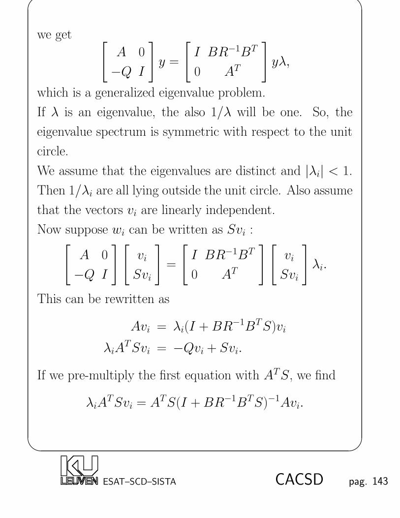
we get [

A 0

−Q I

]

y =

[

I BR−1BT

0 AT

]

yλ,

which is a generalized eigenvalue problem.

If λ is an eigenvalue, the also 1/λ will be one. So, the

eigenvalue spectrum is symmetric with respect to the unit

circle.

We assume that the eigenvalues are distinct and |λi| < 1.

Then 1/λi are all lying outside the unit circle. Also assume

that the vectors vi are linearly independent.

Now suppose wi can be written as Svi :[

A 0

−Q I

][

vi

Svi

]

=

[

I BR−1BT

0 AT

][

vi

Svi

]

λi.

This can be rewritten as

Avi = λi(I + BR−1BTS)vi

λiATSvi = −Qvi + Svi.

If we pre-multiply the first equation with ATS, we find

λiATSvi = ATS(I +BR−1BTS)−1Avi.


'

&

$

%

Now we can eliminate λi to find

(S −Q− ATS(I +BR−1BTS)−1A)vi = 0.

Since the vi are independent, we have

S −Q− ATS(I +BR−1BTS)−1A = 0

and it can be proven, using the matrix inversion lemma1,

that this is the algebraic Riccati equation.

Hence we have found an algorithm to solve the algebraic

Riccati equation :

1. solve the generalized eigenvalue problem[

A 0

−Q I

][

vi

wi

]

=

[

I BR−1BT

0 AT

][

vi

wi

]

λi,

2. let vi and wi correspond to the eigenvalues within the

unit circle,

3. define V = [v1...vN ] and W = [w1...wN ],

4. then

S = WV −1.

1(A+ BCD)−1 = A−1 − A−1B(C−1 +DA−1B)−1DA−1


'

&

$

%

LQR for continuous-time systems

Up till now we restricted ourselves to LQR design for

discrete-time system. A similar procedure exists in con-

tinuous time. We will discuss the results briefly.

The finite-horizon problemBe given a continuous-time system :

x = Ax +Bu, u = −K(t)x

Consider the problem of minimizing the cost function

J =

∫ T

t

(xTQx + uTRu)dτ + xT (T )QTx(T )

with Q, QT and R nonnegative definite weighting matrices

and K(t) the linear system over which the cost function is

going to be minimized.


'

&

$

%

One can prove that the optimal K(t) = R−1BTP (t). P (t)

is the solution to the following Riccati differential equation:

−P = PA + ATP − PBR−1BTP +Q, P (T ) = QT

The infinite-horizon problemNow let t = 0 and T → ∞. The optimal controller is

K = R−1BTP where P is the solution to the continuous

algebraic Riccati equation :

PA + ATP − PBR−1BTP +Q = 0.

Note that P and K are constant matrices now.


'

&

$

%

Algebraic Riccati Equations

Consider the following Riccati equation:

ATX +XA−XBBTX + CTC = 0

Existence, Uniqueness and StabilizabilitySuppose that (A,B) is stabilizable and (A,C) is de-

tectable. Then the Riccati equation has a unique positive

semidefinite solution. Moreover, this solution is stabilizing,

that is,

A−BBTX

has all its eigenvalues in the left half-plane.

Recall that BTX is the state feedback gain K for LQR,

thus the closed loop system with LQR is stable.


'

&

$

%

Elimination of cross terms

So far we used LQR cost functions that made a trade-off

between weighted states x and weighted inputs u. Quite

often however, a trade-off between inputs u and outputs y

is more appropriate.

For continuous-time systems the direct transmission matrix

D is equal to 0 in practice, so y = Cx. A cost function,

making a trade-off between inputs and outputs, can be de-

fined

J =

∫ ∞

0

(yTQy+uTRu)dτ =

∫ ∞

0

(xTCTQCx+uTRu)dτ,

and apparently falls down to equations we already dis-

cussed. Here, Q and R are typically chosen to be diagonal

matrices.

However, in discrete-time the direct transmission matrix D

typically does exist :

yk = Cxk +Duk.

So

yTkQyk = xTkCTQCxk + uTkD

TQDuk + 2xTkCTQDuk,


'

&

$

%

such that J =∑yTkQyk + uTkRuk equals

∞∑

k=0

xTkCTQCxk + uTk (DTQD + R)uk + 2xTkC

TQDuk.

Hence, we have to solve the quadratic function

J =

∞∑

k=0

xTkPxxxk + uTkPuuuk + 2xTkPxuuk.

in which some cross terms do appear. They need to be

eliminated in order to obtain a Riccati equation. Now de-

fine a new input vector vk as (assuming Puu is symmetric

and invertible)

vk = uk + P−1uu P

Txuxk.

Then we find for the state space equations :

xk+1 = (A−BP−1uu P

Txu)xk +Bvk

yk = (C −DP−1uu P

Txu)xk +Dvk

and the cost function is transformed into

J =∞∑

k=0

xTk (Pxx − PxuP−1uu P

Txu)xk + vTk Puuvk

without cross terms. Previously discussed techniques can

now be applied.


'

&

$

%

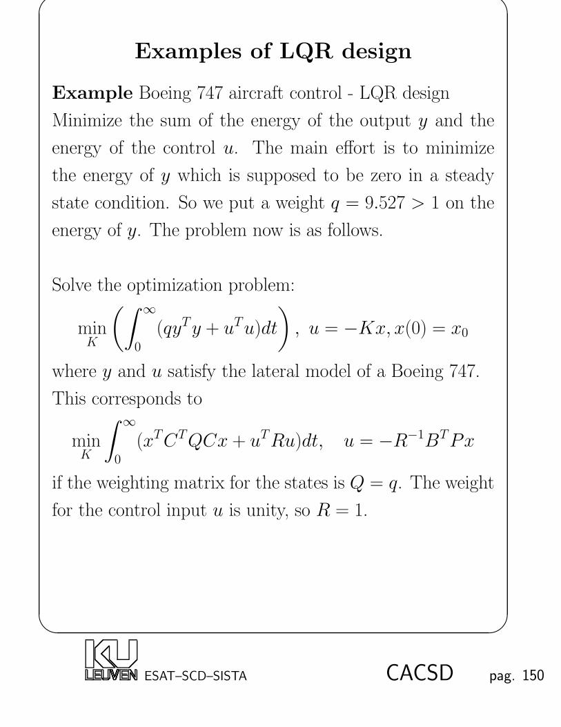
Examples of LQR design

Example Boeing 747 aircraft control - LQR design

Minimize the sum of the energy of the output y and the

energy of the control u. The main effort is to minimize

the energy of y which is supposed to be zero in a steady

state condition. So we put a weight q = 9.527 > 1 on the

energy of y. The problem now is as follows.

Solve the optimization problem:

minK

(∫ ∞

0

(qyTy + uTu)dt

)

, u = −Kx, x(0) = x0

where y and u satisfy the lateral model of a Boeing 747.

This corresponds to

minK

∫ ∞

0

(xTCTQCx + uTRu)dt, u = −R−1BTPx

if the weighting matrix for the states is Q = q. The weight

for the control input u is unity, so R = 1.


'

&

$

%

The Riccati equation

ATP + PA− PBR−1BTP + CTQC = 0

has a solution :

P =

1.06 −0.19 −2.32 0.10 0.04 0.49

−0.19 3.12 0.13 −0.04 0.02 −0.34

−2.32 0.13 5.55 −0.20 −0.08 −1.22

0.10 −0.04 −0.20 0.06 0.03 −0.17

0.04 0.02 −0.08 0.03 0.02 −0.10

0.49 −0.34 −1.22 −0.17 −0.10 1.23

and the feedback control gain

K = R−1BTP =[

1.06 −0.19 −2.32 0.10 0.04 0.49]

.


'

&

$

%

Example Tape drive control - LQR design

The control specification is :

minimize the energy of the output (the position of the

read/write head and the tension at that position) and the

control output. The main purpose is mainly to minimize

the energy of the output which is required to be zero. How-

ever, the control output must not be too large because of

the saturation of the actuator (the drive motor here). Thus

a certain amount of trial and error is usually required to

choose the weighting matrix R and Q.

Let Q = 2I and R = I and solve the Riccati equation

ATP + PA− PBR−1BTP + CTQC = 0.


'

&

$

%

The solution for the Riccati equation is

P =

1.02 1.73 0.84 1.36 0.55 0.45

1.73 4.35 1.36 3.02 1.78 1.14

0.84 1.36 1.02 1.73 0.45 0.55

1.36 3.02 1.73 4.35 1.14 1.78

0.55 1.78 0.45 1.14 0.86 0.46

0.45 1.14 0.55 1.79 0.46 0.86

and thus

K = R−1BTP =

[

0.55 1.78 0.45 1.14 0.86 0.46

0.45 1.14 0.55 1.78 0.46 0.86

]

.

The closed loop poles are at

−0.627± 0.865, −0.406± 0.727i, −1.315, −1.041.


'

&

$

%

Now let Q = 9I and R = I , then the Riccati equation

ATP + PA− PBR−1BTP + CTQC = 0

has a solution:

P =

3.52 4.83 2.84 3.41 1.26 0.86

4.83 9.74 3.41 5.74 3.31 1.68

2.84 3.41 3.52 4.83 0.86 1.26

3.41 5.74 4.83 9.74 1.68 3.31

1.26 3.31 0.86 1.68 1.39 0.53

0.86 1.68 1.26 3.31 0.53 1.39

so the state feedback gain:

K = R−1BTP =

[

1.26 3.31 0.86 1.68 1.39 0.53

0.86 1.68 1.26 3.31 0.53 1.39

]

.

The closed loop poles are:

−0.784± 1.174, −0.574± 0.907, −1.596, −1.158.


'

&

$

%

The output impulse responses:

0 5 10 15 20

0

0.1

0.2

Input1/Output1

0 5 10 15 20−0.2

−0.15

−0.1

−0.05

0

0.05Input1/Output2

0 5 10 15 20

0

0.1

0.2

Input2/Output1

0 5 10 15 20−0.05

0

0.05

0.1

0.15

0.2Input2/Output2

Dashed line: Q = 2I

Solid line: Q = 9I

The larger Q, the faster and smaller the transient.

(What is the price for a larger Q?)


'

&

$

%

The control output impulse responses:

0 5 10 15 20−0.5

0

0.5

1

1.5input1/control1

0 5 10 15 20−0.2

0

0.2

0.4

0.6Input1/control2

0 5 10 15 20−0.2

0

0.2

0.4

0.6Input2/control1

0 5 10 15 20−0.5

0

0.5

1

1.5Input2/control2

Dashed line: Q = 2I

Solid line: Q = 9I

The larger Q, the larger the control output u.


'

&

$

%

Matlab Functions

are

dare

dlqr

dlqry

lqr

lqry

quadprog

rlocus


'

&

$

%

Chapter 5

Estimator Design - Pole placement

Motivation

• Control law design with state feedback needs all the

state variables.

• Not all state variables are available since the cost of

the required sensors may be prohibitive, or it may be

physically impossible to measure all the state variables.

Estimator: reconstruct all the state variables x of a system

from measurements. The reconstructed state variables x

are then used for control.


'

&

$

%

Motivation example

Example Boeing 747 aircraft control

In the Boeing 747 aircraft model, there are 4 states : the

side-slip angle β, the yaw rate r, the roll rate p and the roll

angle φ. Only the yaw rate r is measured with a gyroscope,

while all other states are not measured.

Challenge : Can we estimate the states β, p and φ from the

measurement of r such that the state feedback control law

can be implemented? What are the effects of the estimated

states on the final closed loop system?


'

&

$

%

Full Order Estimators (Observers)

Open loop estimatorEstimator:

Reconstruct a full order model of the plant dynamics:

˙x = Ax + Bu.

x is the estimate of the state x.

The dynamics of this estimator:

Define the error in the estimate:

x∆= x− x

Then the dynamics of this error system are given by (sub-

tracting the estimate from the state):

˙x = Ax, x(0) = x(0)− x(0).


'

&

$

%

˙x = Ax+ Bu

x = Ax+ Buu

Process

Estimator

xC

x

y

Disadvantage of the open loop estimator:

• The error is converging to zero at the same rate as the

natural dynamics of A (if A is stable). There is no

way to influence the rate at which the state estimate

converges to the true state.

• The error will NOT converge if A is unstable.

• If the model dynamics (A,B,C,D) are different from

the system dynamics (due to inaccurate modeling for

instance), in general, x will not converge to 0.


'

&

$

%

Estimator with feedback

Estimator:

Insert the feedback signal of the difference between the mea-

sured and estimated outputs (y−Cx) to correct the model:

˙x = Ax +Bu + L(y − Cx).

where L is a constant matrix in Rn×p.

Dynamics of the estimator:

The error dynamics are given as follows (by subtracting the

estimate from the state):

˙x = (A− LC)x, x(0) = x(0)− x(0).


'

&

$

%

x = Ax+Bu

Process

˙x = Ax+Bu+ Ly

Estimator

C

C

−

+

y

y

u x

x

y

Properties:

• By choosing the gain matrix L, the error dynamics of

A − LC can be stable and much faster than the open

loop dynamics A.

• In case of inaccurate A and/or C, the error dynamics

can still be stabilized and be faster ⇒ Robustness.


'

&

$

%

Estimator Design - Pole Placement

Choose the gain matrix L

such that the poles of the

estimator are in desired

positions.

Let the desired locations be given by

s = s1, s2, . . . , sn

then the desired estimator characteristic equation is

αe(s)∆= (s− s1)(s− s2) . . . (s− sn)

Direct methodDetermine L by comparing coefficients of the two polyno-

mials on both sides of the following equation :

det (sI − (A− LC)) = (s− s1)(s− s2) . . . (s− sn)


'

&

$

%

Duality of estimation and control designsThe problem to find L such that

det (sI − (A− LC)) = (s− s1)(s− s2) . . . (s− sn)

is equivalent to the problem to find K = LT such that

det(sI − (AT − CTK)

)= (s− s1)(s− s2) . . . (s− sn)

which is the problem for state feedback control design.

Further, the controllability matrix C of (A,B) is the trans-

pose of the observability matrix O of (AT , BT ). Thus we

have the following duality relations:

Control Estimation

A AT

B CT

K LT

C OT


'

&

$

%

Ackermann’s formula for SISO

L = αe(A)O−1

0

0...

1

where O is the observability matrix.

Sylvester equation for MIMO:Design procedure:

• Pick an arbitrary matrix G ∈ Rp×n.

• Solve the Sylvester equation for X :

ATX −XΛ = CTG

Λ =

α1 β1

−β1 α1

. . .

λ1

. . .

,

which has eigenvalues: α1± jβ1, . . . , λ1, . . . . which are

the desired poles of the estimator.

• Obtain the static feedback gain L = (GX−1)T .


'

&

$

%

Estimator Pole Selection

The dynamics of the state estimation error are governed

by the eigenvalues of A − LC. Obviously, all eigenvalues

are chosen to be stable. Concerning the estimator pole se-

lection there is a fundamental trade-off between sensitivity

of the estimation error to sensor noise and speed of con-

vergence. The smaller Reeig(A − LC), the faster the

estimation error goes to zero. However, for small eigenval-

ues rapid changes in the signals will also introduce rapid

changes in the estimation error. The estimated state will

change nervously. In the next chapter we will describe an

optimal solution for this dilemma which is the Kalman fil-

ter.

Consider a control system with process noise w and sensor

noise v:

x = Ax +Bu +B1w,

y = Cx + v

then the estimator error will be :

˙x = (A− LC)x +B1w − Lv


'

&

$

%

Rules of thumb:• Trade-off between a fast dynamic response (of the esti-

mator) and a good sensor noise reduction. ⇒ “large”

L or “small ” L.

• Trade-off between process noise reduction and sensor

noise reduction. ⇒ “large” L or “small ” L.

Consider the following first order system

x = −x + u

y = x + v

where v is sensor noise.

Now compare 2 estimators : A−LC = −10 and A−LC =

−2. There is no input, but the initial state is 1. The

dynamics for A − LC = −10 are faster but more subject

to noise :

0 0.5 1 1.5 2 2.5 3 3.5 4 4.5 5−0.2

0

0.2

0.4

0.6

0.8

1

1.2

time (s)

− state evolution

−− estimated state, A−LC=−10

.. estimated state, A−LC=−2


'

&

$

%

Examples of estimator design

Example Boeing 747 aircraft control - Estimator design

with pole placement (Ackermann’s method)

We have designed a state feedback control law, and the

desired closed-loop poles are at

−0.0051, −0.468, −1.106, −9.89, −0.279± 0.628i.

For a fast response of the estimator, we make the poles of

the estimator 5 times faster than the desired closed-loop

poles :

−0.0255, −2.34 ,−5.53, −49.45, −1.395± 3.14i.

The characteristic polynomial of the estimator

αe(s) = s6 + 60.14s5 + 575.4s4 + 2453s3 + 6595s2 + 7721s + 192.6

αe(A) =

−1.13e+ 6 0 0 0 0 0

−4.48e+ 4 −5.15e+ 3 −4.49e+ 3 6.01e+ 2 2.24e+ 2 0

−5.38e+ 5 3.27e+ 3 −4.06e+ 3 1.91e+ 2 1.50e+ 2 0

1.81e+ 5 −8.17e+ 3 1.55e+ 4 −3.62e+ 3 −6.12e+ 2 0

−1.72e+ 4 −1.45e+ 4 8.58e+ 3 4.54e+ 3 −6.54e+ 1 0

5.38e+ 4 3.17e+ 3 3.84e+ 3 −3.14e+ 1 5.48e+ 1 −1.73e+ 3


'

&

$

%

The observability matrix equals

O =

0 0 1 0 0 −3.33e− 1

−4.75e+ 0 5.98e− 1 −4.48e− 1 −3.18e− 2 0 1.11e− 1

4.96e+ 1 −2.04e− 1 −4.46e− 1 7.70e− 2 2.48e− 2 −3.70e− 2

−4.94e+ 2 −4.90e− 1 2.50e− 1 −1.32e− 2 −8.49e− 3 1.23e− 2

4.94e+ 3 2.17e− 1 4.66e− 1 −4.96e− 2 −2.03e− 2 −4.12e− 3

−4.94e+ 4 4.18e− 1 −2.95e− 1 5.31e− 3 9.01e− 3 1.37e− 3

Then the feedback gain for the estimator is

L =

2.5047e + 01

−2.0517e + 03

−5.1935e + 03

−2.4851e + 04

−4.0914e + 04

−1.5728e + 04


'

&

$

%

Example Tape drive control - Estimator design with pole

placement (Sylvester equation)

The desired estimator poles are again set to be 5 times

faster than the desired closed-loop poles:

−2.2550±4.6850i, −4.7350±2.9050i, −5.8000, −5.8000.

Take an arbitrary matrix G:

G =

[

−0.508 −0.248 −0.445 −0.209 −1.064 1.133

0.885 −0.726 −0.613 0.562 0.352 0.150

]

Solve the Sylvester equation for X :

ATX −XΛe = CTG

Λe is a block diagonal matrix with the eigenvalues equal to

the desired estimator poles:

Λc =

−2.225 4.685

−4.685 −2.225

−4.735 2.905

−2.905 −4.735

−5.8

−5.8

.


'

&

$

%

X =

−4.0150e − 02 −7.4418e − 02 −3.5794e − 02 −2.4713e − 02 −1.0413e − 01 9.2375e − 02

−6.1041e − 02 3.7229e − 03 2.4053e − 02 −3.0478e − 02 2.4528e − 02 −3.8791e − 02

4.0795e − 02 −3.4260e − 02 −5.2180e − 02 3.4518e − 02 −7.9299e − 02 1.0297e − 01

2.1710e − 02 1.2860e − 02 1.5984e − 03 9.5250e − 03 4.1517e − 02 −3.1544e − 02

2.9984e − 03 8.9685e − 03 −4.3541e − 05 6.1539e − 03 −3.8326e − 03 6.0611e − 03

1.0521e − 03 −3.7573e − 03 −1.1269e − 03 −1.0362e − 03 −6.4870e − 03 4.9287e − 03

Now obtain the estimator feedback gain L = X−TGT :

L =

5.38e + 01 −4.21e + 01

2.04e + 02 −1.56e + 02

3.90e + 01 −7.92e + 00

4.00e + 02 −3.08e + 02

6.51e + 02 −5.82e + 02

1.77e + 03 −1.50e + 03


'

&

$

%

Matlab Functions

obsv

poly

real

polyvalm

acker

lyap

place


'

&

$

%

Chapter 6

Optimal Estimator - Kalman Filter

Formulation

We want to control the following discrete-time system by

state feedback

xk+1 = Axk +B2uk +B1wk

yk = C2xk +D2uk + vk

So far, we know how to design a gain matrix K by pole

placement or LQR. The states are not measured, but esti-

mated by a state observer. Its dynamics are controlled by

a matrix L.

A fast observer reacts more nervously to the measurement

noise v, whereas a slow state estimator may be less sensi-

tive to v, but amplifies the process noise w.

If the characteristics of the noise sources w and v are known

in advance an optimal state estimator can be designed.

This optimal state estimator or Kalman filter will be stud-

ied in this chapter.


'

&

$

%

Discrete-time Kalman filtering

Least squares formulationConsider a discrete-time system

xk+1 = Axk +B2uk +B1wk

yk = C2xk +D2uk + vk.

At a certain time k, the state space equations can be as-

sembled in a large over-determined set of linear equations,

with a vector of unknowns θ containing all previous state

vectors, up to xk+1 :

−B2u0

y0 −D2u0

−B2u1

y1 −D2u1

...

−B2uk

yk −D2uk

︸︷︷︸

b

=

A −IC2 0

A −IC2 0

. . .

A −IC2 0

︸︷︷︸

A

x0

x1

x2

...

xk

xk+1

︸︷︷︸

θ

+

B1w0

v0

B1w1

v1

...

B1wk

vk

︸︷︷︸

e


'

&

$

%

We have to find an optimal state vector estimate θ that is

the ’best’ solution for the set of equations

b = Aθ + e.

Vector e contains stacked and weighted noise samples wk

and vk. We assume that the characteristics of w and v are

known and are such that

E(e) = 0 : zero-mean

E(eeT) = W

W is the so-called noise covariance matrix, which in this

case gives some information about the amplitude of the

noise components, their mutual correlation and spectral

shaping (correlation in time domain).

If the components of both w and v are stationary, mutually

uncorrelated and white, having the same variance σ2w and

σ2v respectively,

W =

σ2wB1B

T1 0 0 . . . 0

0 σ2vI 0 . . . 0

0 0 σ2wB1B

T1 . . . 0

... . . . . . . . . . ...

0 0 0 . . . σ2vI


'

&

$

%

The optimal estimate for θ can be found as

θ = (ATW−1A)−1ATW−1b

θ is the least squares solution to

minθ(b−Aθ)TW−1(b−Aθ)

based on input-output data up to time k.

Disadvantage: k →∞ ⇒ dimension of A→∞.


'

&

$

%

Recursive least squares problemFinite horizon case :How can we find an optimal estimate xk+1|k, in the least

squares sense, for the state xk+1, by making use of observa-

tions of inputs u and outputs y up to time k, given xk|k−1,

the estimate for xk at time k − 1 ?

Consider the following state observer

xk+1|k = Axk|k−1 +B2uk + Lk(yk − C2xk|k−1 −D2uk).

Combining it with the system equations leads to the esti-

mator error equation

xk+1|k = xk+1− xk+1|k = (A−LkC2)xk|k−1 +B1wk−LkvkWe will assume that wk and vk have zero-mean white noise

characteristics with covariance

E(wjwTk ) = Qδjk,

E(vjvTk ) = Rδjk,

E(vjwTk ) = 0

and Q and R nonnegative definite weighting matrices.


'

&

$

%

Our aim now is to find an optimal estimator gain Lk that

minimizes

αTPk+1α = αTE((xk+1 − E(xk+1))(xk+1 − E(xk+1))T )α.

α is an arbitrary column vector. Pk is called the estimation

error covariance matrix.

From the estimator error equation and taking in account

the properties of the noise :

E(xk+1) = (A− LkC2)E(xk).

Now if we take E(x0) = 0, the mean value of the estimation

error is zero for all k. Then,

Pk+1 = E((xk+1)(xk+1)T )

= (A− LkC2)Pk(A− LkC2)T + B1QB

T1 + LkRL

Tk

So, if P0 is properly set, Pk will be symmetric positive

semidefinite for all k .


'

&

$

%

The optimal Lk or Kalman filter gain can be obtained by

minimizing

Lk = argminLk

αTPk+1α.

Setting the derivative with respect to Lk equal to zero,

αT (−2APkCT2 + 2Lk(R + C2PkC

T2 ))α = 0.

The equality has to be fulfilled for all vectors α, so

Lk = APkCT2 (R + C2PkC

T2 )−1.

and the error covariance update equation becomes

Pk+1 = APkAT+B1QB

T1−APkCT

2 (R+C2PkCT2 )−1C2PkA

T

which is a Riccati difference equation.


'

&

$

%

Infinite horizon case :It can be shown that if the system is controllable and ob-

servable and k →∞, matrix Pk converges to a steady-state

positive semidefinite matrix P and Lk approaches a con-

stant matrix L with

L = APCT2 (R + C2PC

T2 )−1.

P satisfies the Discrete Algebraic Riccati Equation :

P = B1QBT1 + APAT − APCT

2 (R + C2PCT2 )−1C2PA

T

Both for the finite horizon and the infinite horizon case,

the Kalman filter equations are similar to the equations we

obtained for LQR design.


'

&

$

%

Verify the duality relation between Kalman filter design and

LQR by using the following conversion table and plugging

in the correct matrices in the LQR equations.

Conversion table

LQR ↔ Kalman filter design

LQR Kalman filter

A AT

B CT2

Q B1QBT1

K LT

Kalman filters may be designed based on LQR formulas

using this table, as is done in Matlab for instance. The

Kalman filter is sometimes referred to as LQE, i.e. a Linear

Quadratic Estimator.


'

&

$

%

Continuous-time Kalman filtering

Consider a system:

x = Ax +B2u +B1w,

y = C2x +D2u + v

and the estimator:

˙x = Ax + L(y − C2x−D2u) +B2u

where the input disturbance noise w and the sensor noise

v are zero mean white noise with covariance Q and R re-

spectively.

Find an optimal L such that the following stochastic cost

function

E

1

T

∫ T

0

((x− x)T (x− x)dt

)

is minimized.


'

&

$

%

Finite-horizon case :This leads to the Riccati differential equation :

−P = PAT +AP −PCT2 R−1C2P +B1QB

T1 , P (0) = 0.

The optimal estimator or Kalman gain :

L = P (t)CT2 R−1

Infinite-horizon case :This leads to the continuous Algebraic Riccati equation :

PAT + AP − PCT2 R−1C2P +B1QB

T1 = 0

and the corresponding Kalman gain :

L = PCT2 R−1

Duality with LQR design :Also for the continuous time case the conversion rules on

page 182 hold.


'

&

$

%

Examples of Kalman Filter Design

Example Boeing 747 aircraft control - Kalman Filter

Suppose the plant noise w enters the system in the same

way as the control input and suppose the measurement

noise is v. Then

x = Ax +Bu +B1w,

y = Cx +Du + v.

where (A,B,C,D) is the nominal aircraft model given in

the previous examples. B1 = B =[

1 0 0 0 0 0]T

. Sup-

pose further that w and v are white noises with the covari-

ance of w, Rw = 0.7 and the covariance of v Rv = 1.

The Riccati equation

QAT + AQ−QCTR−1v CQ +B1RwB

T1 = 0


'

&

$

%

has a solution:

Q=

3.50e− 2 1.94e− 3 −1.60e− 2 2.88e− 3 −3.08e− 4 −1.55e− 3

1.94e− 3 5.20e− 1 3.68e− 2 −9.45e− 1 3.43e+ 0 −3.88e− 2

−1.60e− 2 3.68e− 2 8.18e− 1 −6.79e− 1 1.34e+ 1 1.78e+ 0

2.88e− 3 −9.45e− 1 −6.79e− 1 5.06e+ 0 −1.03e+ 0 1.59e− 1

−3.08e− 4 3.43e+ 0 1.34e+ 1 −1.03e+ 0 3.51e+ 2 4.12e+ 1

−1.55e− 3 −3.88e− 2 1.78e+ 0 1.59e− 1 4.12e+ 1 5.33e+ 0

and the Kalman filter gain is

L = QCTR−Tv =

−1.5465e− 02

4.9686e− 02

2.2539e− 01

−7.3199e− 01

−3.0200e− 01

−8.2157e− 15

.

Now we can compare this result with the result from pole

placement discussed in the previous chapter.

The Kalman Filter has poles at

−9.992, −0.1348± 0.9207i, −0.5738, −0.0070, −0.352

They are slower than those from pole placement, but the

Kalman filter is less (actually least) sensitive to the noises.


'

&

$

%

Example Tape drive control - Kalman filter design

Suppose again that the plant noise w enters the system in

the same way as the control input and suppose that the

measurement noise is v. Then

x = Ax +Bu +B1w,

y = Cx +Du + v.

where (A,B,C,D) is the nominal model given in the pre-

vious examples and

B1 = B =

[

0 0 0 0 1 0

0 0 0 0 0 1

]T

.

Suppose that the RMS accuracy of the tape position mea-

surement is 2 · 10−5 m and the RMS accuracy of tension

measurement is 0.01 N. This means the covariance matrix

of v is

Rv =

[

4 · 10−10 0

0 0.0001

]

.

The covariance matrix of w is given as

Rw =

[

0.001 0

0 0.001

]

.


'

&

$

%

The following Riccati equation

QAT + AQ−QCTR−1v CQ +B1RwB

T1 = 0

has as solution :

Q=

2.23e− 1 3.16e− 3 2.22e− 1 3.02e− 3 2.39e− 4 1.07e− 4

3.16e− 3 4.81e− 4 3.02e− 3 3.35e− 4 2.22e− 4 5.33e− 5

2.22e− 1 3.02e− 3 2.23e− 1 3.16e− 3 1.07e− 4 2.39e− 4

3.02e− 3 3.35e− 4 3.16e− 3 4.81e− 4 5.33e− 5 2.22e− 4

2.39e− 4 2.22e− 4 1.07e− 4 5.33e− 5 4.75e− 4 1.65e− 5

1.07e− 4 5.33e− 5 2.39e− 4 2.22e− 4 1.65e− 5 4.75e− 4

and the Kalman filter gain is

L = QCT2 R−Tv =

5.56e− 02 −1.67e + 00

7.74e− 04 −5.71e− 01

5.56e− 02 1.67e + 00

7.74e− 04 5.71e− 01

4.32e− 05 −6.02e− 01

4.32e− 05 6.02e− 01

.

The Kalman filter poles are at

−0.5882± 0.9226i, −1.1695, −0.0633 ,−0.2735 ,−0.969.

Again these poles are slower, but less sensitive to the noise

than those used in the pole placement design example from

a previous chapter.


'

&

$

%

Matlab Functions

are

dkalman

dlqe

kalman

lqe


'

&

$

%

Chapter 7

Compensator Design

Compensator Structure

Compensator = Control Law + Estimator

−K˙x = Ax+ B2u

+L(y − C2x)

x = Ax+B2u

+B1wy = C2x+ v

x

w v

u

Control law Estimator

y

Process

Compensator

x


'

&

$

%

Standard Plant Formulation

In control theory the following general system description,

called standard plant, is often used

+ + +

uk

vk

yk

wk

zk

B1

B2

C1

C2

D1

D2

z−1

A

xk+1 = Axk +B1wk +B2uk

yk = C2xk +D2uk + vk

zk =

[

C1xk

D1uk

]

where xk is the state vector, zk is the regulated output

vector, yk is the measurement vector, uk is the control in-

put, wk and vk are process noise and measurement noise

respectively.


'

&

$

%

Clearly there are 2 types of inputs :

• the actuator or control input uk : inputs manipulated

by the compensator

• the exogeneous input wk : all other input signals

and 2 types of outputs :

• measured output yk : inputs to the compensator

• regulated output zk : all outputs that are of interest for

control. These outputs may be virtual and not mea-

sured. They typically define the state feedback cost

function

JN =N∑

k=0

zTk zk =N∑

k=0

(xTkCT1 C1xk + uTkD

T1D1uk)

so, using the LQR formalism, by definition of zk,

Q = CT1 C1 and R = DT

1D1.


'

&

$

%

State-space Description

Plant :

xk+1 = Axk +B2uk + B1wk,

zk =

[

C1xk

D1uk

]

,

yk = C2xk +D2uk + vk.

Estimator :

xk+1 = Axk + L(yk − C2xk −D2uk) + B2uk.

Control law :

uk = −Kxk.

Compensator :

xk+1 = (A−B2K − LC2 + LD2K)xk + Lyk,

uk = −Kxk.


'

&

$

%

Closed-Loop System

A state-space model for plant + compensator is

[

xk+1

xk+1

]

=

[

A −B2K

LC2 A− B2K − LC2

][

xk

xk

]

+

[

B1 0

0 L

][

wk

vk

]

,

yk =[

C2 −D2K][

xk

xk

]

+[

0 I][

wk

vk

]

.

Using the error system (estimator) dynamics

xk+1 = (A− LC2)xk +B1wk − Lvk,

we obtain

[

xk+1

xk+1

]

=

[

A−B2K B2K

0 A− LC2

][

xk

xk

]

+

[

B1 0

B1 −L

][

wk

vk

]

,

yk =[

C2 −D2K D2K][

xk

xk

]

+[

0 I][

wk

vk

]

.


'

&

$

%

Separation Principle:Pole Placement

The characteristic equation of the closed-loop system

det

[

sI − A +B2K −B2K

0 sI − A + LC2

]

= 0

The poles of the closed-loop system can be obtained from

det(sI − A + BK) det(sI − A + LC) = αc(s)αe(s) = 0

⇒ Separation Principle (for Pole Placement):

The set of poles of the

closed-loop system consists

of the union of the control

poles and estimator poles.


'

&

$

%

Design procedure :

• Choose the desired poles for the state feedback control

loop. Determine the control law K via pole placement.

• Choose the desired poles for the estimator. Determine

the estimator feedback gain L via pole placement.

• Combine the estimator and the control law to get the

final compensator.


'

&

$

%

Linear Quadratic Gaussian Control

Measurement feedback controlLet w and v be Gaussian zero mean white noises.

Our aim is to find an output feedback controller u = Ky

such that

limT→∞

1

T

∫ T

0

zTzdt

or limK→∞

1

K

K∑

k=0

zTk zk

is minimized.

This problem is called the Linear Quadratic Gaussian

(LQG) control problem.

The difference between LQG and LQR is that LQR uses

state feedback and hence K is just a constant matrix while

LQG uses measurement or output feedback and hence K

is a dynamic system.


'

&

$

%

Stochastic Separation Principle

It can be proven that the solution

to the LQG optimal control prob-

lem consists in using the optimal

state estimator (Kalman filter) to-

gether with the same feedback as

would have been applied had the

states been measured (LQR). This

principle relies on the assumption

of linearity, the Gaussian charac-

ter of the noise and the use of a

quadratic optimization criterion.


'

&

$

%

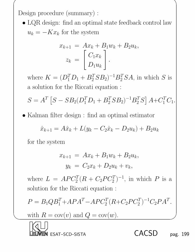
Design procedure (summary) :

• LQR design: find an optimal state feedback control law

uk = −Kxk for the system

xk+1 = Axk +B1wk +B2uk,

zk =

[

C1xk

D1uk

]

.

where K = (DT1D1 + BT

2 SB2)−1BT

2 SA, in which S is

a solution for the Riccati equation :

S = AT[S − SB2(D

T1D1 +BT

2 SB2)−1BT

2 S]A+CT

1 C1.

• Kalman filter design : find an optimal estimator

xk+1 = Axk + L(yk − C2xk −D2uk) +B2uk

for the system

xk+1 = Axk +B1wk +B2uk,

yk = C2xk +D2uk + vk,

where L = APCT2 (R + C2PC

T2 )−1, in which P is a

solution for the Riccati equation :

P = B1QBT1 +APAT−APCT

2 (R+C2PCT2 )−1C2PA

T .

with R = cov(v) and Q = cov(w).


'

&

$

%

• Combination of the LQR control law and the Kalman

filter : the final controller K is given as follows :


uk = −Kxk.

Design strategy for LQG :

Trade-off between speed of time responses and

attenuation of noises by choosing the covariance

matrices of w and v.

Similarly,

Trade-off between the energy of the states and energy

of the control effort by choosing the weighting matrices

CT1 C1 and DT

1D1.


'

&

$

%

Compensator Dynamics

Compensator :


uk = −Kxk.

Characteristic equation of the compensator :

det(zI − A +B2K + LC2 − LD2K) = 0

⇒The poles of the compensator are not necessary in the unit

circle, the compensator might be unstable.

Transfer function of the compensator :

K(z) = −K(zI − A +B2K + LC2 − LD2K)−1L.


'

&

$

%

Summary of State Space Control

Design

LQG

compensator design

system modeling

LQR Kalman filter pole placementpole placement

pole placement

control law design estimator design


'

&

$

%

Examples of Compensator Design

Example Boeing 747 Aircraft control - Compensator de-

sign

The complete model of the aircraft is

x = Ax +Bu +Bw,

z =

[

q1/2Cx

u

]

,

y = Cx + v.

where q is the weighting factor and w and v are zero

mean white noises with covariance Rw and Rv respectively.

(A,B,C,D) is the nominal aircraft model (D = 0).


'

&

$

%

First, we design a compensator via pole placement. From

results of pole placement design examples in chapter 3 and

chapter 5, we know that the state feedback gain

K =[

1.06 −0.19 −2.32 0.10 0.04 0.49]

places the poles of the control loop at

−0.0051, −0.468, −1.106, −9.89, −0.279± 0.628i

and the estimator gain

L =

2.5047e + 01

−2.0517e + 03

−5.1935e + 03

−2.4851e + 04

−4.0914e + 04

−1.5728e + 04

places the estimator poles at

−0.0255, −2.34 ,−5.53, −49.45, −1.395± 3.14i.

The compensator then is

˙x = (A−BK − LC)x + Ly,

u = −Kx.


'

&

$

%

The poles of the compensator are then at

−51.35, −4.074± 10.12i, −0.8372± 0.6711i, −0.027.

So the compensator itself is stable, which is preferred since

otherwise an accident resulting in a breakdown of the

control loop will cause the control output to go to infinity.

The transfer function of the compensator K(s) is

K(s) = −K(sI − A +BK + LC)−1L

= 102 −8.42s5 − 92.3s4 − 72.1s3 + 74.9s2 + 113s + 2.55

s6 + 61.2s5 + 640s4 + 7086s3 + 11029s2 + 7316s+ 194.


'

&

$

%

The initial condition response with β0 = 1 :

0 5 10 15 20 25 30 35 40 45 50−4

−2

0

2

4

6

8

10

12x 10

−3

Time (secs)

r(ra

d/s

ec)

The response is almost the same as with state feedback

control but with a slightly larger peak value and with the

slowly decaying error (see the plot on page 97) filtered out

here.


'

&

$

%

Now consider LQG design. Let q = 9.527, Rw = 0.7 and

Rv = 1. From the results of LQR and Kalman filter design

examples in chapter 4 and 6, we obtained a state feedback

gain K

K =[

1.06 −0.19 −2.32 0.10 0.04 0.49]

and an estimator gain

L =

−1.5465e− 02

4.9686e− 02

2.2539e− 01

−7.3199e− 01

−3.0200e− 01

−8.2157e− 15

.

The poles of the compensator with the K and L above are

at:

−9.845, −1.405, −0.2616± 0.5571i, −0.4756, −0.0049.

Again the compensator is stable.


'

&

$

%


0 5 10 15 20 25 30 35 40 45 50−8

−6

−4

−2

0

2

4

6

8

10

12x 10

−3

Time (secs)

r(ra

d/s

ec)

This initial condition response shows that the Kalman filter

is too slow compared with the state feedback control loop.


'

&

$

%

The reason for this result is that the measurement noise v

is large compared with the process noise w, so that the

Kalman filter has to reduce the measurement noise in-

fluence using a small estimator L, which slows down the

Kalman filter. Now increase the process noise covariance

to Rw = 700. The Kalman filter gain is now

L =

−8.0289e + 00

−3.3434e− 01

8.2913e + 00

−4.8082e + 00

−3.4682e + 00

3.5982e− 11

The poles of the compensator are at

−9.845, −1.405, −0.2616± 0.5571i, −0.4756, −0.0049.


'

&

$

%

It’s not clear whether or not the Kalman filter is speeding

up from these poles location. But the following initial

condition response shows that the result is much better.


0 5 10 15 20 25 30 35 40 45 50−3

−2

−1

0

1

2

3

4

5

6

7x 10

−3

Time (secs)

r(ra

d/s

ec)

This response is even better than the one from pole place-

ment and with a better noise attenuation.


'

&

$

%

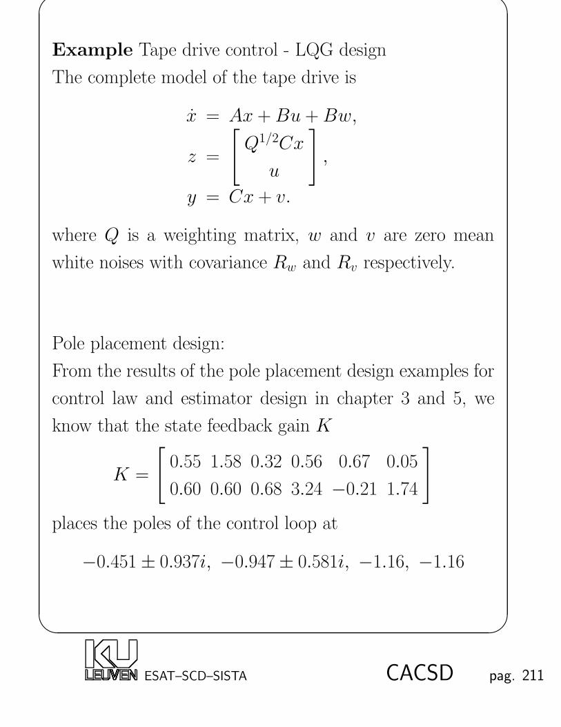
Example Tape drive control - LQG design

The complete model of the tape drive is

x = Ax +Bu +Bw,

z =

[

Q1/2Cx

u

]

,

y = Cx + v.

where Q is a weighting matrix, w and v are zero mean

white noises with covariance Rw and Rv respectively.

Pole placement design:

From the results of the pole placement design examples for

control law and estimator design in chapter 3 and 5, we

know that the state feedback gain K

K =

[

0.55 1.58 0.32 0.56 0.67 0.05

0.60 0.60 0.68 3.24 −0.21 1.74

]

places the poles of the control loop at

−0.451± 0.937i, −0.947± 0.581i, −1.16, −1.16


'

&

$

%

and the estimator gain

L =

5.3833e + 01 −4.2084e + 01

2.0377e + 02 −1.5615e + 02

3.9038e + 01 −7.9226e + 00

4.0009e + 02 −3.0809e + 02

6.5103e + 02 −5.8228e + 02

1.7691e + 03 −1.5000e + 03

places the estimator poles at

−2.255± 4.685i, −4.735± 2.905i, −5.800, −5.800.

The compensator then is

˙x = (A−BK − LC)x + Ly,

u = −Kx.


'

&

$

%

The compensator has poles at

−1.696± 8.531, −12.09, −5.847, −3.335± 0.2469i.

The initial condition response with x1(0) = x3(0) = 1 looks

like

0 1 2 3 4 5 6 7 8 9 10−1

−0.8

−0.6

−0.4

−0.2

0

0.2

0.4

0.6

0.8

1

Time (secs)

Am

plitu

de

p3

T


'

&

$

%

Now consider LQG design.

Let

Q = 2I2, Rw = 0.001I4, Rv =

[

4 0

0 0.0001

]

.

From the results of the LQR and Kalman filter design ex-

amples in chapter 4 and 6, we obtain the optimal state

feedback gain K

K =

[

0.55 1.78 0.45 1.14 0.86 0.46

0.45 1.14 0.55 1.78 0.46 0.86

]

and the optimal estimator gain

L =

5.56e− 02 −1.67e + 00

7.74e− 04 −5.71e− 01

5.56e− 02 1.67e + 00

7.74e− 04 5.71e− 01

4.32e− 05 −6.02e− 01

4.32e− 05 6.02e− 01

.


'

&

$

%

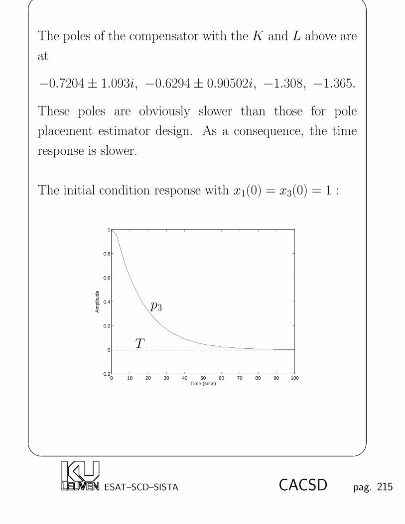
The poles of the compensator with the K and L above are

at

−0.7204± 1.093i, −0.6294± 0.90502i, −1.308, −1.365.

These poles are obviously slower than those for pole

placement estimator design. As a consequence, the time

response is slower.

The initial condition response with x1(0) = x3(0) = 1 :

0 10 20 30 40 50 60 70 80 90 100−0.2

0

0.2

0.4

0.6

0.8

1

Time (secs)

Am

plitu

de

p3

T


'

&

$

%

Matlab Functions

initial

kalman

lqg

lqgreg

lqr

reg


'

&

$

%

Chapter 8

Reference Introduction – Integral

Control

Reference Input – Zero Design

Motivation

A controller obtained by combining a control law with an

estimator is essentially a regulator design : the charac-

teristic equations of the controller and the estimator are

basically chosen for good disturbance rejection. However,

it does not lead to tracking, which is evidenced by a good

transient response of the combined system to command

changes. A good tracking performance is obtained by

properly introducing the reference input into the system.

This is equivalent to design proper zeros from the reference

input to the output.


'

&

$

%

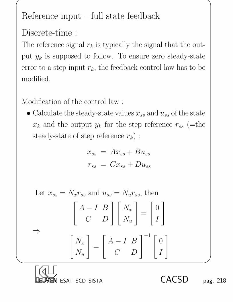
Reference input – full state feedback

Discrete-time :The reference signal rk is typically the signal that the out-

put yk is supposed to follow. To ensure zero steady-state

error to a step input rk, the feedback control law has to be

modified.

Modification of the control law :

• Calculate the steady-state values xss and uss of the state

xk and the output yk for the step reference rss (=the

steady-state of step reference rk) :

xss = Axss +Buss

rss = Cxss +Duss

Let xss = Nxrss and uss = Nurss, then[

A− I B

C D

][

Nx

Nu

]

=

[

0

I

]

⇒ [

Nx

Nu

]

=

[

A− I B

C D

]−1 [

0

I

]


'

&

$

%

• Modify the control law:

uk = Nurk−K(xk−Nxrk) = −Kxk+(Nu +KNx)︸︷︷︸

N

rk

In this way the steady-state error to a step input will be 0.

Proof :

1. Verify that the closed-loop system from rk to yk is given

by[

xk+1

xk+1

]

=

[

A −BKLC A−BK − LC

][

xk

xk

]

+

[

BN

BN

]

rk,

yk =[

C −DK][

xk

xk

]

+DNrk.

2. If |eig(A−BK)| < 1 and |eig(A−LC)| < 1 we obtain

the following steady-state equations :

xss = Axss −BKxss + BNrss

xss = xss

yss = (C −DK)xss +DNrss

uss = −Kxss + Nrss

⇓yss = Cxss +D(−Kxss + Nrss) = Cxss +Duss = rss


'

&

$

%

So the transfer matrix relating y and r is a unity matrix

at DC ⇒ zero steady–state tracking error, steady–state

decoupling.

Note that:

• rk is an exogenous signal, the reference introduction will

NOT affect the poles of the closed-loop system.

•[

A− I B

C D

]−1

must exist, and thus for MIMO

number of references = number of outputs

• also for MIMO, reference introduction implies a steady-

state decoupling between different reference and output

pairs. This means that yss = rss.

• some properties of this controller are discussed on page

227.

Continuous-time :Try to verify that in this case

[

Nx

Nu

]

=

[

A B

C D

]−1 [

0

I

]


'

&

$

%

There are two types of interconnections for reference input

introduction with full state-feedback :

Type I: uk = Nurk −K(xk −Nxrk)

Type II: uk = −Kxk + (Nu +KNx)︸︷︷︸

N

rk

-

+-

+

-

+

EstimatorEstimator

PlantPlant

xx

rr uu y y

K K

Nu

Nx

N

For a type II interconnection, the control lawK used in the

feedback (uk = −Kxk) and in the reference feedforward

(N = Nu + KNx) should be exactly the same, otherwise

there is a steady-state error. There is no such problem in

type I.

⇒Type I is more ROBUST to parameter errors than Type

II.


'

&

$

%

Reference Input - General Compensator

Plant and compensator model :

Plant : xk+1 = Axk +Buk,

yk = Cxk +Duk;

Compensator : xk+1 = (A−BK − LC + LDK)xk

+Lyk,

uk = −KxkThe structure of a general compensator with reference in-

put r :

N

−K

M

yu

r +

+

xEstimator

Process


'

&

$

%

The general compensator is defined by the following closed-

loop equations from rk to yk :[

xk+1

xk+1

]

=

[


][

xk

xk

]

+

[

BN

M

]

rk,

yk =[

C −DK][

xk

xk

]

+DNrk.

Hence, the equations defining the compensator are

xk+1 = (A−BK − LC + LDK)xk + Lyk

+(M − LDN)rk,

uk = −Kxk + Nrk

where M ∈ Rn×m and N ∈ R

p×m.

The estimator error dynamics are

xk+1 = (A− LC)xk +BNrk −Mrk.


'

&

$

%

Poles:

Characteristic equation:

det

(

zI −[


])

= 0.

This is the same characteristic equation as without ref-

erence introduction. So introducing references will NOT

change the poles.

Zeros :

The equations for a transmission zero are (see page 82)

det

ζI − A BK −BN−LC ζI − A +BK + LC −MC −DK DN

= 0

⇔

ζI − A BK −BN−LC ζI − A +BK + LC −MC −DK DN

u

v

w

︸︷︷︸6=0

= 0

⇔


'

&

$

%

det

[

ζI − A −BC D

]

det

[

ζI − A +BK + LC −M−K N

]

= 0

The first term determines the transmission zeros of the open

loop system while the second term corresponds to the trans-

mission zeros of the compensator from rk to uk:

xk+1 = (A−BK − LC + LDK)xk + (M − LDN)rk,

uk = −Kxk + Nrk

These transmission zeros are designed via reference intro-

duction.


'

&

$

%

Autonomous estimator (cfr. pag. 218-220) :

Select M and N such that the state estimator error equa-

tion is independent of r ⇒

M = BN

where N is determined by the method for introducing the

reference input with full state feedback.

−K

y

r +

xEstimator

Process

+

u

N


'

&

$

%

Zeros :

The transmission zeros from rk to uk in this case are deter-

mined by

det(ζI − A + LC) = 0

which is the characteristic equation for the estimator, hence

the transmission zeros from rk to uk cancel out the poles

of the state estimator.

Properties :

• The compensator is in the feedback path. The refer-

ence signal rk goes directly into both the plant and the

estimator.

• Because of the pole-zero cancelation which causes “un-

controllability” of the estimator modes, the poles of the

transfer function from rk to yk consist only of the state

feedback controller poles (the roots of det(sI − A +

BK) = 0).

• The nonlinearity in the input (saturation) cancels out in

the estimator since in this case the state estimator error

equation is independent of u (xk+1 = (A− LC)xk)


'

&

$

%

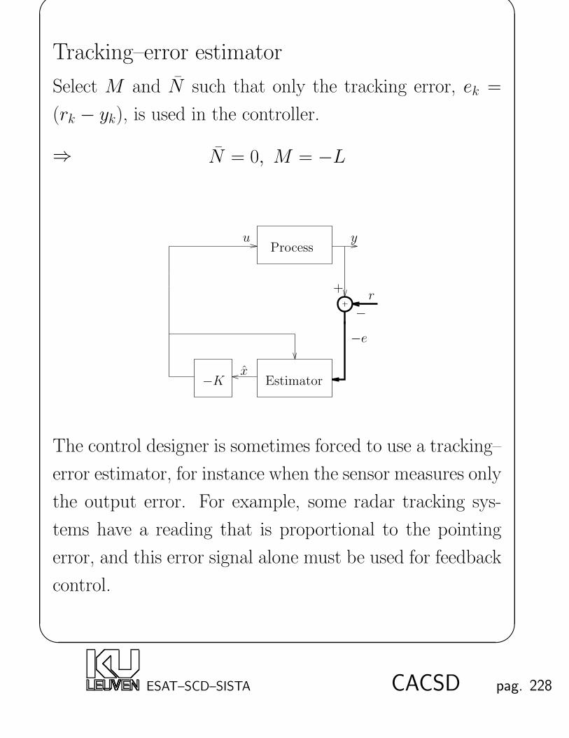
Tracking–error estimator

Select M and N such that only the tracking error, ek =

(rk − yk), is used in the controller.

⇒ N = 0, M = −L

−K

y

xEstimator

Processu

r+

−−e

The control designer is sometimes forced to use a tracking–

error estimator, for instance when the sensor measures only

the output error. For example, some radar tracking sys-

tems have a reading that is proportional to the pointing

error, and this error signal alone must be used for feedback

control.


'

&

$

%

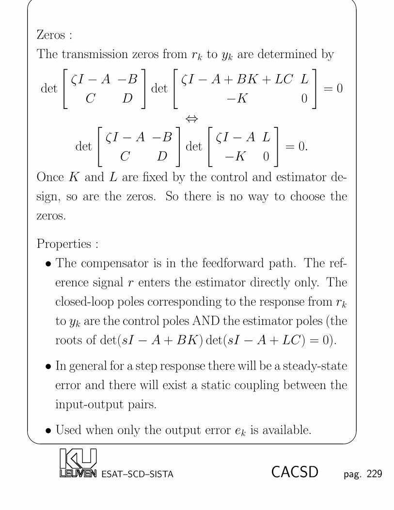
Zeros :

The transmission zeros from rk to yk are determined by

det

[

ζI − A −BC D

]

det

[

ζI − A +BK + LC L

−K 0

]

= 0

⇔

det

[

ζI − A −BC D

]

det

[

ζI − A L

−K 0

]

= 0.

Once K and L are fixed by the control and estimator de-

sign, so are the zeros. So there is no way to choose the

zeros.

Properties :

• The compensator is in the feedforward path. The ref-

erence signal r enters the estimator directly only. The

closed-loop poles corresponding to the response from rk

to yk are the control poles AND the estimator poles (the

roots of det(sI − A + BK) det(sI − A + LC) = 0).

• In general for a step response there will be a steady-state

error and there will exist a static coupling between the

input-output pairs.

• Used when only the output error ek is available.


'

&

$

%

Zero-assignment estimator (SISO) :

Select M and N such that n of the zeros of the overall

transfer function are placed at desired positions. This

method provides the designer with the maximum flexibil-

ity in satisfying transient-response and steady-state gain

constraints. The previous two methods are special cases of

this method.

Zeros of the system from rk to uk:

det

[

ζI − A +BK + LC −M−K N

]

= 0

⇓ M∆= MN−1

λ(ζ)∆= det(ζI − A + BK + LC − MK) = 0


'

&

$

%

Solution :

Determine M using a estimator pole-placement strategy

for “system” (Az, Cz), with

Az = A− BK − LC, Cz = K,

N is determined such that the DC gain from rk to yk is

unity.

For instance, in the case of a SISO system in continuous

time, for which D = 0

N = − 1

C(A−BK)−1B[1−K(A− LC)−1(B − M)]

and finally M = MN .


'

&

$

%

Example Tape drive control - reference introduction

Autonomous Estimator :

Consider the model of the tape drive on page 39. From the

pole-placement design example on page 114, K is known.[

A B

C D

]−1 [

0

I

]

=

[

1 0 1 0 0 0 0 0

−2.5 0 2.5 0 −0.67 0.67 −0.67 0.67

]T

.

Thus,

Nx =

1 −2.5

0 0

1 2.5

0 0

0 −0.67

0 0.67

, Nu =

[

0 −0.67

0 0.67

]

.


'

&

$

%

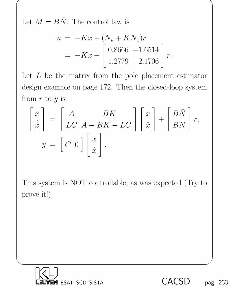
Let M = BN . The control law is

u = −Kx + (Nu +KNx)r

= −Kx +

[

0.8666 −1.6514

1.2779 2.1706

]

r.

Let L be the matrix from the pole placement estimator

design example on page 172. Then the closed-loop system

from r to y is[

x˙x

]

=

[

A −BKLC A− BK − LC

][

x

x

]

+

[

BN

BN

]

r,

y =[

C 0][

x

x

]

.

This system is NOT controllable, as was expected (Try to

prove it!).


'

&

$

%

Step responses from the reference r to the output y.

0 2 4 6 8 10 12 14 16 18 20−0.5

0

0.5

1

1.5

Time (secs)

Am

plitu

de

0 2 4 6 8 10 12 14 16 18 20−0.5

0

0.5

1

1.5

Time (secs)

Am

plitu

de

T

T

p3

p3

Step input to reference 1

Step input to reference 2

Output 1 (p3) follows a step input to reference 1 while

output 2 (T ) is zero in steady state.

Output 2 (T ) follows a step input to reference 2 while

output 1 (p3) is zero in steady state.

⇒ steady-state decoupling.


'

&

$

%

Integral Control and Robust Tracking

Motivation:The choice of N will result in a step response with a zero

steady-state error (see page 218). But the result is not

robust because any change in the parameters will cause the

error to be nonzero. Integral control is needed to obtain

robust tracking of step inputs.

A more general method for robust tracking, called the error

space approach (see page 238), can solve a broader class of

tracking problems, i.e. tracking signals that do not go to

zero in steady-state (a step, ramp, or sinusoidal signal).


'

&

$

%

Integral control

Augment the plant

xk+1 = Axk +Buk,

yk = Cxk +Duk

with extra states integrating the output error ek = yk− rkxIk+1

= xIk+ Cxk +Duk − rk︸︷︷︸

ek

.

The augmented state equations become[

xIk+1

xk+1

]

=

[

I C

0 A

][

xIk

xk

]

+

[

D

B

]

uk −[

I

0

]

rk.

What are the equivalent equations in continuous-time ?

We now close the loop to stabilize the system. The feedback

law is

uk = −[

K1 K0

]

︸︷︷︸K

[

xIk

xk

]

.


'

&

$

%

Use pole placement or LQR methods to design the control

feedback gain K. Once the closed-loop is stable, the track-

ing error e goes to zero even if some parameters change.

Processr y

+

−+

+−K1u

x

1z−1

−K0

The states of the plant xk are estimated using a state es-

timator. The estimator gain L is determined using pole

placement or Kalman filtering techniques. The integrator

states xIk need not to be estimated as they are being com-

puted explicitly.

What will be the closed-loop response from rk to yk ? Try

to derive a state-space model.

Note that pole placement or LQR might not work since the

augmented system is NOT always stabilizable and in this

case integral control can not be used.


'

&

$

%

Tracking control - the error-space approach

Integral control is limited to step response tracking. A

more general approach, the error-space approach, gives a

control system the ability to track a non-decaying or even

a growing input such as a step, a ramp, or a sinusoid.

Suppose the external signal, the reference, is generated by a

certain dynamic system. By including the dynamic system

as a part of the formulation and solving the control problem

in an error space, the error approaches zero.


'

&

$

%

Given the plant dynamics

xk+1 = Axk +Buk,

yk = Cxk +Duk

and the reference dynamics

rk+2 + α1rk+1 + α2rk = 0,

the tracking error is defined as

ek = yk − rk.


'

&

$

%

Define the error-space state:

ξk∆= xk+2 + α1xk+1 + α2xk,

and the error-space control:

µk = uk+2 + α1uk+1 + α2uk.

Then

ek+2 + α1ek+1 + α2ek = Cξk +Dµk,

and the state equation for ξk becomes

ξk+1 = Aξk +Bµk

Combining these two equations, the final error system is

zk+1 = Aezk +Beµk

where

zk =

ek

ek+1

ξk

, Ae =

0 I 0

−α2I −α1I C

0 0 A

, Be =

0

D

B

.


'

&

$

%

Controllability of the error system:

If (A,B) is controllable and has no zero at the roots of

αe(z) = z2 + α1z + α2,

then (Ae, Be) is controllable.

Control design: Pole-placement or LQR

µk = −[

K2 K1 K0

]

ek

ek+1

ξk

= −Kzk

The actual control uk is determined by the following inter-

nal model:

(u +K0x)k+2 +2∑

i=1

αi(u +K0x)k+2−i = −2∑

i=1

Kiek+2−i.

Once the closed-loop is stable, ek and ek+1 go to zero even

if some parameters change.


'

&

$

%

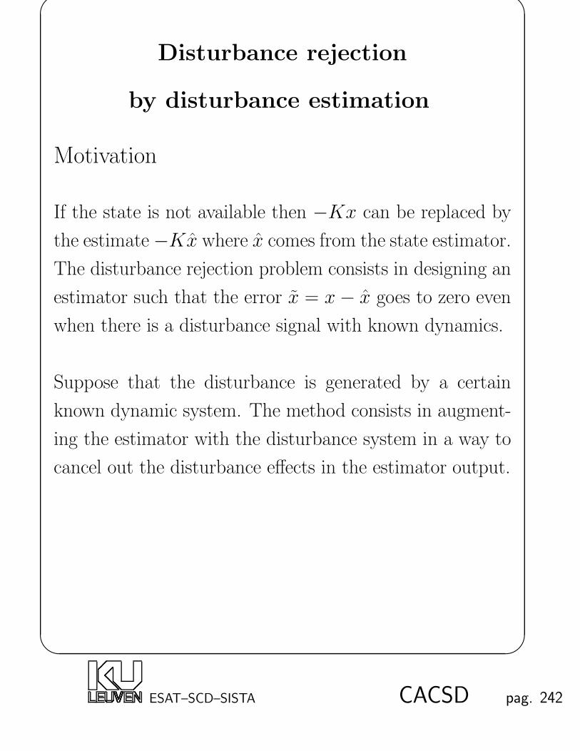
Disturbance rejection

by disturbance estimation

Motivation

If the state is not available then −Kx can be replaced by

the estimate−Kx where x comes from the state estimator.

The disturbance rejection problem consists in designing an

estimator such that the error x = x− x goes to zero even

when there is a disturbance signal with known dynamics.

Suppose that the disturbance is generated by a certain

known dynamic system. The method consists in augment-

ing the estimator with the disturbance system in a way to

cancel out the disturbance effects in the estimator output.


'

&

$

%

Augmenting the disturbance system to the plant

Given a plant with a disturbance input:

xk+1 = Axk +B(uk + wk),

yk = Cxk +Duk

and the disturbance dynamics (suppose 2nd order):

wk+2 + α1wk+1 + α2wk = 0.

The final error system is

zk+1 = Adzk +Bduk

where

z =

wk

wk+1

xk

, Ad =

0 I 0

−α2I −α1I 0

B 0 A

, Bd =

0

0

B

,

Cd =[

D 0 C]

, Dd = D.


'

&

$

%

Observability:

If the plant (A,C) is observable and has no zero at any

roots of

αd(z) = z2 + α1z + α2,

then (Ad, Cd) is observable.

Estimator for the error system:

zk+1 = Adzk + Bduk + L(yk − Cdzk −Dduk).

The output uk:

uk = −Kxk + Nrk︸︷︷︸

introduce reference

− wk︸︷︷︸cancel disturbance

.

Final closed-loop system:

xk+1 = (A− BK)xk + BNrk +BKxk + Bwk.

where xk = xk − xk and wk = wk − wk.

Stable estimator ⇒ xk → 0 and wk → 0. The final state

is NOT affected by the disturbance.


'

&

$

%

Chapter 9

Sensitivity - Robustness

Why robustness?

• The plant characteristics may be variable or time-

varying. System modeling techniques identify the plant

within a certain model class and with a certain amount

of inaccuracy. So there always exists a plant uncer-

tainty, which can not be described exactly by the math-

ematical models.

• Control systems need to be made robust against this

plant variability and uncertainty.

Why frequency response analysis?

• There is a clear connection between frequency response

plots and experimentally obtained data.

• Easy to learn for trained engineers familiar with classi-

cal frequency response methods.


'

&

$

%

Sensitivity

DefinitionSensitivity of a quantity α to changes in a quantity β:

Sαβ∆=∂α

∂β· βα

=∂α/∂β

α/β.

⇒A measure of the relative change in α due to a relative

change in β.

Sensitivity for a SISO system:

gt(s)k(s)r yc

gt(s): plant, k(s): controller.


'

&

$

%

The closed-loop transfer function from r to yc:

h(s) =gt(s)k(s)

1− gt(s)k(s).

The sensitivity of h(s) to changes in gt(s):

Shg (s) =∂h(s)

∂gt(s)

gt(s)

h(s)=

1

1− gt(s)k(s)

Plant variations will have a small or a large effect on the

closed-loop transfer function according to the size of the

sensitivity function (1− gt(s)k(s))−1.

⇒The robustness of the closed-loop system to plant variations

is improved by making the sensitivity function small, said

otherwise, by making the “loop gain” gt(s)k(s) large.


'

&

$

%

Sensitivity for a MIMO system:

Consider the following two control systems :

Gt(s)K(s)r yc

controllerequivalent

K(s) Gt(s)

G(s)

yor

The equivalent open loop, G(s): model,

Gt(s): plant with uncertainties, K(s): controller.

Since

yc = Gt(s)K(s)(I −Gt(s)K(s))−1r,

yo = Gt(s)K(s)(I −G(s)K(s))−1r.

it follows that yc = yo for all r if the system Gt(s) and the

model G(s) are identical.


'

&

$

%

Suppose the plant Gt(s) depends on a parameter δ. Then,

∂yc∂δ

= (I −Gt(s)K(s))−1

×∂Gt(s)

∂δK(s)(I −Gt(s)K(s))−1r,

∂yo∂δ

=∂Gt(s)

∂δK(s)(I −G(s)K(s))−1r.

Assume G(s) = Gt(s)|δ=δnom, then

∂yc∂δ

∣∣∣∣δ=δnom

= (I −Gt(s)K(s))−1 ∂yo∂δ

∣∣∣∣δ=δnom

.

⇒The sensitivity operator

S(s)∆= (I −Gt(s)K(s))−1

determines how changes in the plant affect the output of the

closed-loop scheme given changes in the nominally equiva-

lent open-loop scheme.

For matrices :

if y = Su

⇓||y|| ≤ σmax(S)||u||


'

&

$

%

Again, the closed-loop scheme will be more or less sensitive

to changes in the output depending on the “size” of S(s):∥∥∥∥

∂yc(jω)

∂δ

∥∥∥∥δ=δnom

≤ σ(S(jω))

∥∥∥∥

∂yo(jω)

∂δ

∥∥∥∥δ=δnom

.

where σ(S(jω)) is the largest singular value of the matrix

S(jω), a measure for the matrix size, and ‖ · ‖ is the

2-norm of a vector.

A feedback or controller design objective might be:

σ(S(jω)) < 1, ∀ω

which ensure that the closed-loop scheme is uniformally

less sensitive to changes in system parameters than the

open-loop scheme.

Complementary sensitivity:

T (s)∆= G(s)K(s)S(s) = G(s)K(s)(I −G(s)K(s))−1

Note that S + T = I . The complementary sensitivity will

be used later.


'

&

$

%

Robust Stability Analysis

Nyquist stability

Consider the following feedback system

w u

y d

G(s)

K(s)

Definition for internal stability :

Suppose G(s) and K(s) are propera rational transfer func-

tion matrices and let H(s) denote the closed-loop transfer

function matrix from

[

w

d

]

to

[

u

y

]

:

H(s) =

[

I −K(s)

−G(s) I

]−1

.

Then

• The feedback loop is called well posed if H(s) is proper.

• The feedback loop is internally stable if H is stable.aH(s) is proper iff lims→∞ H(s) = D and D is finite. If D = 0, H(s) is called strictly proper.


'

&

$

%

Nyquist stability criterion for MIMO systems:

Let G(s) and K(s) be given proper rational transfer func-

tions that form a well-posed closed loop, and let G(s) and

K(s) have nG and nK poles (counting multiplicities) re-

spectively in the closed-right half plane. The feedback

loop is internally stable if and only if the Nyquist diagram

Γ = det(I − G(s)K(s)) makes nG + nK anti-clockwise

encirclements around the origin (without crossing it) for

s ∈ DR, where DR is the Nyquist contour:

x

x

r

jω

R

x: poles of G(s) or K(s) on the imaginary axis.

R is large enough to contain all the closed right half plane

poles of G(s), K(s) and H(s).


'

&

$

%

Small Gain Theorem

Gain of a system H

||H||gn = sup||w||6=0

||Hw||||w||

here ||.|| is your favorite, well-chosen norm.

Not all norms will do : not every system norm is a gain.

Some gains for instance have the property that they are

finite if and only if the system is stable :

||H||gn <∞⇔ H is stable.

The H∞-norm is an example.

Sub-multiplicativityFor all gains, the gain of a cascade is not larger than the

product of the gains

||H1H2||gn ≤ ||H2||gn||H1||gn.

This is called sub-multiplicativity.


'

&

$

%

Small Gain Theorem

Consider the following system :

++ +

H1

H2

zw

Assume the problem is well-posed i.e. det(I −H1H2) 6= 0.

Then the transfer matrix from w to z is

Gzw = (I −H1H2)−1H1

Now the small gain theorem states :

If ||H1||gn||H2||gn < 1, then

||Gzw||gn ≤||H1||gn

1− ||H1||gn||H2||gn

If ||.||gn is such that finiteness means stability, then the

small gain condition ||H1||gn||H2||gn < 1 implies stability

of Gzw.


'

&

$

%

Proof :

we have

z = H1(w +H2z) = H1w +H1H2z

The triangle inequality delivers

||z|| ≤ ||H1w||+ ||H1H2z||

Using the gain definitions & sub-multiplicativity

||z|| ≤ ||H1||gn||w||+ ||H1H2||gn||z||≤ ||H1||gn||w||+ ||H1||gn||H2||gn||z||

so that

||z||(1− ||H1||gn||H2||gn) ≤ ||H1||gn||w||.

From the small gain condition

||H1||gn||H2||gn < 1

we find

||z|| ≤ ||H1||gn1− ||H1||gn||H2||gn

||w||.


'

&

$

%

Additive model errorConsider the control system:

∆a(s)

G(s)

K(s)

Feedback loop with additive model error

G(s): Nominal system transfer function,

∆a(s): Additive stable perturbation transfer function,

K(s): Controller transfer function designed to ensure the

internal stability of the nominal closed-loop.

How large can σ(∆a(jω)) become before the closed-loop

becomes unstable?


'

&

$

%

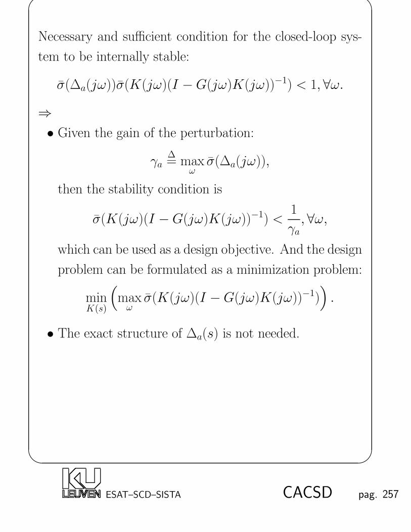
Necessary and sufficient condition for the closed-loop sys-

tem to be internally stable:

σ(∆a(jω))σ(K(jω)(I −G(jω)K(jω))−1) < 1, ∀ω.

⇒• Given the gain of the perturbation:

γa∆= max

ωσ(∆a(jω)),

then the stability condition is

σ(K(jω)(I −G(jω)K(jω))−1) <1

γa,∀ω,

which can be used as a design objective. And the design

problem can be formulated as a minimization problem:

minK(s)

(

maxωσ(K(jω)(I −G(jω)K(jω))−1)

)

.

• The exact structure of ∆a(s) is not needed.


'

&

$

%

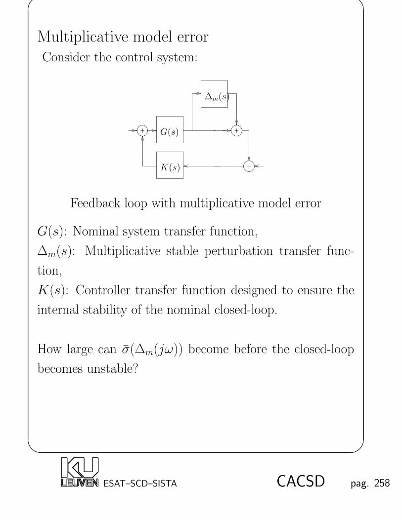
Multiplicative model errorConsider the control system:

∆m(s)

G(s)

K(s)

Feedback loop with multiplicative model error


∆m(s): Multiplicative stable perturbation transfer func-

tion,



How large can σ(∆m(jω)) become before the closed-loop

becomes unstable?


'

&

$

%



σ(∆m(jω))σ(G(jω)K(jω)(I −G(jω)K(jω))−1

︸︷︷︸T (jω)

) < 1,∀ω.

⇒• Given the gain of the perturbation:

γm∆= max

ωσ(∆m(jω)),


σ(T (jω)) <1

γm,∀ω

which can be used as a design objective. And the design

problem can be formulated as a minimization problem:

minK(s)

(

maxωσ(T (jω))

)

.

• The exact structure of ∆m(s) is again not needed.


'

&

$

%

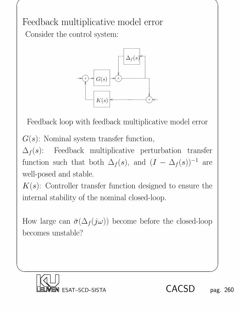
Feedback multiplicative model errorConsider the control system:

G(s)

K(s)

∆f(s)

Feedback loop with feedback multiplicative model error


∆f(s): Feedback multiplicative perturbation transfer

function such that both ∆f(s), and (I − ∆f(s))−1 are

well-posed and stable.



How large can σ(∆f(jω)) become before the closed-loop

becomes unstable?


'

&

$

%



σ(∆f(jω))σ((I −G(jω)K(jω))−1

︸︷︷︸S(jω)

) < 1, ω ∈ R.

⇒• Given the gain of the perturbation

γf∆= max

ωσ(∆f(jω)),


σ(S(jω)) <1

γf, ∀ω,

which can be used as an design objective, and the design

problem can be formulated as

minK(s)

(

maxωσ(S(jω))

)

.

• The exact structure of ∆f(s) is not needed.


'

&

$

%

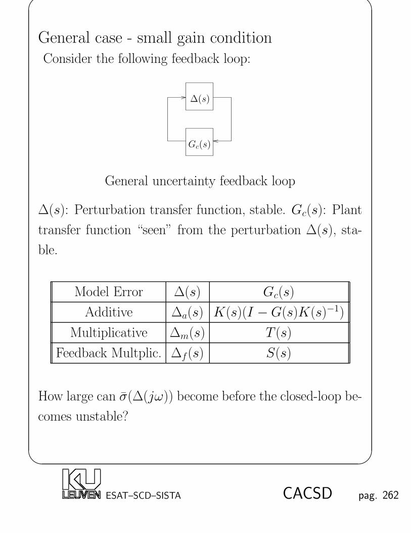
General case - small gain conditionConsider the following feedback loop:

∆(s)

Gc(s)

General uncertainty feedback loop

∆(s): Perturbation transfer function, stable. Gc(s): Plant

transfer function “seen” from the perturbation ∆(s), sta-

ble.

Model Error ∆(s) Gc(s)

Additive ∆a(s) K(s)(I −G(s)K(s)−1)

Multiplicative ∆m(s) T (s)

Feedback Multplic. ∆f(s) S(s)

How large can σ(∆(jω)) become before the closed-loop be-

comes unstable?


'

&

$

%

Small Gain Condition:


tem to be internally stable (page 254) :

σ(∆(jω))σ(Gc(jω)) < 1, ∀ω.

⇒• Essentially the small gain condition states that if a feed-

back loop consists of stable systems and the loop-gain

product is less than unity, then the feedback loop is in-

ternally stable. Otherwise there always exists a ∆(s)

such that the closed-loop system is unstable.

• Given the gain of the perturbation

γ∆= max

ωσ(∆(jω)),


σ(Gc(jω)) <1

γ,∀ω

• There is no need to know the structure of the pertur-

bation ∆(s).


'

&

$

%

Example Tape drive control - Robustness analysis

Since only robust stability will be investigated here, all

the noise inputs, the reference input and the regulated

output are neglected and only the main loop (LQG design

here) will be considered:

LQG controller K(s)

∆f(s)∆m(s)

∆a(s)

Tape drive G(s)

We analyze how large the additive, multiplicative and feed-

back multiplication perturbations (∆a(s),∆m(s),∆f(s))

would be before the system becomes unstable when they

are independently acting in the closed-loop.


'

&

$

%

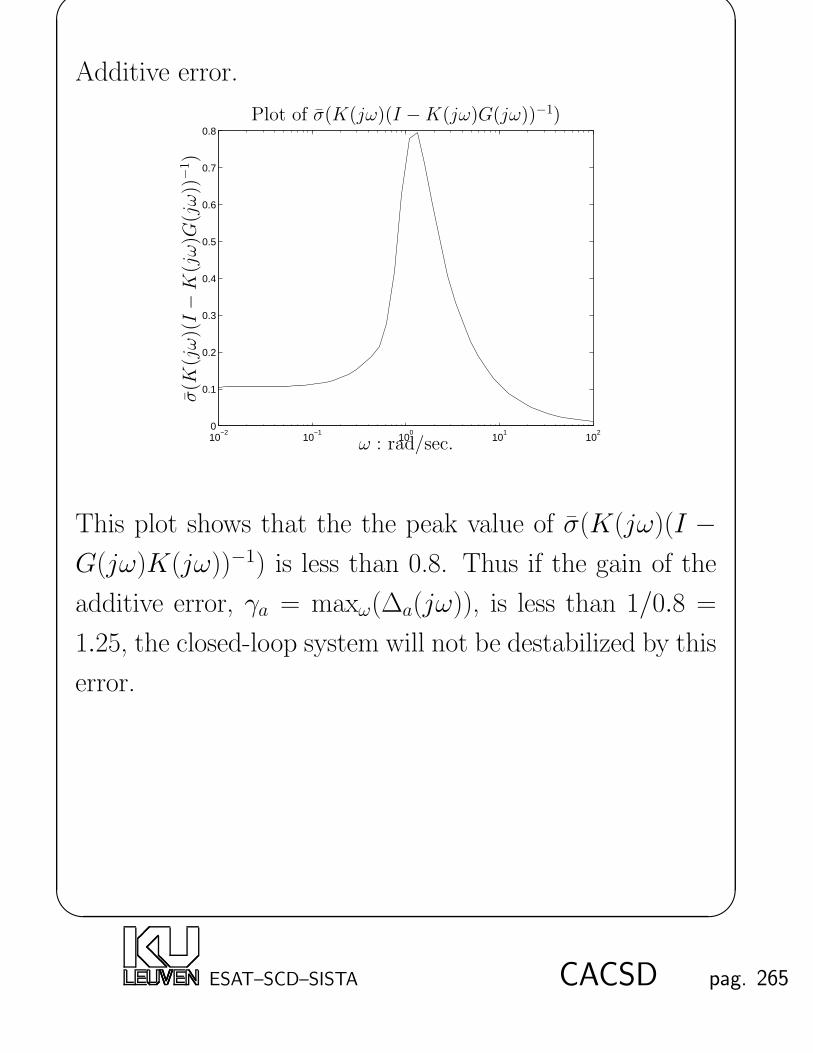
Additive error.

10−2

10−1

100

101

102

0

0.1

0.2

0.3

0.4

0.5

0.6

0.7

0.8Plot of σ(K(jω)(I −K(jω)G(jω))−1)

σ(K

(jω)(I−K

(jω)G

(jω))−

1)

ω : rad/sec.

This plot shows that the the peak value of σ(K(jω)(I −G(jω)K(jω))−1) is less than 0.8. Thus if the gain of the

additive error, γa = maxω(∆a(jω)), is less than 1/0.8 =

1.25, the closed-loop system will not be destabilized by this

error.


'

&

$

%

Multiplicative error.

10−2

10−1

100

101

102

0

0.2

0.4

0.6

0.8

1

Complementary sensitivity plot

σ(T

)

ω : rad/sec.

This plot shows that the peak value of the maximum sin-

gular value of the complementary sensitivity is less than

1. Thus once the gain of the multiplicative error, γm =

maxω(∆m(jω)), is less than 1, the closed-loop system will

not be destabilized by this error.


'

&

$

%

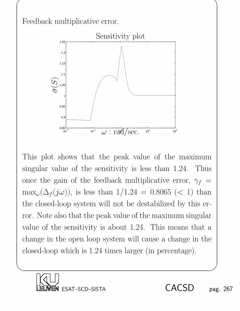
Feedback multiplicative error.

10−2

10−1

100

101

102

0.85

0.9

0.95

1

1.05

1.1

1.15

1.2

1.25

Sensitivity plot

σ(S

)

ω : rad/sec.

This plot shows that the peak value of the maximum

singular value of the sensitivity is less than 1.24. Thus

once the gain of the feedback multiplicative error, γf =

maxω(∆f(jω)), is less than 1/1.24 = 0.8065 (< 1) than

the closed-loop system will not be destabilized by this er-

ror. Note also that the peak value of the maximum singular

value of the sensitivity is about 1.24. This means that a

change in the open loop system will cause a change in the

closed-loop which is 1.24 times larger (in percentage).


'

&

$

%

Summary

• Using SVD as a vehicle to analyze the robustness of

systems with perturbations gives a simple way to gen-

eralize the frequency analysis methods from SISO to

MIMO systems. However, since the structures of the

perturbations are not considered, the results are often

conservative. Thus it is possible that some classes of

perturbations with specific structure (diagonal for in-

stance) might never destabilize the closed-loop systems

even if the gain conditions are not satisfied.

• So far we have not discussed the subject on robust con-

trol design, which is out of the scope of this course.

Robust control design for systems with unstructured

perturbations, namely H∞ control synthesis, has been

solved. The structure of the solution is similar to LQG

control: combine the optimal control law and optimal

estimator based on a similar separation principle as in

LQG design. However, the Riccati equations are differ-

ent.


'

&

$

%

Table of Contents

CACSD 1

Practical information about the course 2

”Eindtermen” 5

List of references 6

Chapter 1 : Introduction 13

3 Motivating Examples 15

Glass oven 15

Boeing 747 aircraft control 22

CVT control 26

General control configuration 29

Systems and models 30

Chapter 2 : State Space Models 34

State space models 34

Tape drive control example 36

Transfer matrix and impulse response 40

Linearization 41

Digitization 49

Geometric properties of linear state space models 60

Canonical forms 60

Uniqueness 63

Controllability 64

Observability 66

Popov-Belevitch-Hautus test 68

Stability, stabilizability and detectability 70

Kalman decomposition 72

Minimal realization 75

Input/output properties of state space models 76


'

&

$

%

Poles 76

Second-order system 79

Transmission zeros 82

Example of state space analysis 87

Matlab functions 92

Chapter 3 : Pole Placement 93

State feedback 93

Pole placement 100

Direct method 102

Ackermann’s method 103

Sylvester equation 108

Examples 111

Transmission zeros 116

Pole location selection 117

Dominant second-order poles 117

Prototype design 118

Matlab functions 124

Chapter 4 : Linear Quadratic Regulator 125

Quadratic minimization 125

Least squares 125

Constrained minimization : basics of MPC 127

Linear Quadratic Regulator 132

LQR for discrete-time systems 135

Lagrange multipliers method 135

Sweep method 137

Solving the algebraic Riccati equation 142

LQR for continuous-time systems 145

Elimination of cross terms 148

Examples 150



'

&

$

%

Chapter 5 : Estimator design - pole placement 158

Observers 158

Open loop estimator 161

Estimator with feedback 162

Estimator design - pole placement 164

Direct method 164

Ackermann’s method 166

Sylvester equation 166

Estimator pole selection 167

Rules of thumb 168

Examples 169


Chapter 6 : Kalman filter 174

Discrete-time Kalman filtering 174

Least-squares formulation 175

Recursive least-squares problem 178

Continuous-time Kalman filtering 183

Examples 185


Chapter 7 : Compensator Design 190

Compensator structure 190

Standard plant 191

State-space description 193

Separation principle : pole placement 195

Linear Quadratic Gaussian Control 197

Stochastic separation principle 198

Design strategy for LQG 200

Compensator dynamics 201

Summary of state space control design 202


'

&

$

%

Examples 203


Chapter 8 : Reference Introduction - Integral Control 217

Reference introduction 217

Nu and Nx 218

Two types of interconnections 221

General compensator 222

Compensator zeros 224

Autonomous estimator 226

Tracking-error estimator 228

Zero-assignment estimator 230

Example 232

Integral Control 235

Error-space approach 238

Disturbance rejection 242

Chapter 9 : Sensitivity - Robustness 245

Motivation 245

Sensitivity 246

for SISO 246

for MIMO 248

Robust stability analysis 251

Nyquist stability 251

Small gain theorem 253

Additive model error 256

Multiplicative model error 258

Feedback multiplicative model error 260

Small gain condition 262

Example 264

Summary 268

Table of Contents 269


Documents

Computer Aided Control System Designmaapc/static/files/CACSD/... · 2018-02-07 · ∗AutoCode (automatic generation of C-code) ... Design controllers such that the closed-loop system