Computations via experiments with kinematicsystems1

E.J. Beggs2 and J.V. Tucker3

University of Wales Swansea,Singleton Park,

Swansea, SA3 2HN,United Kingdom

Abstract

Consider the idea of computing functions using experiments with kinematic sys-tems. We prove that for any set A of natural numbers there exists a 2-dimensionalkinematic system BA with a single particle P whose observable behaviour decidesn ∈ A for all n ∈ N. The system is a bagatelle and can be designed to operate under(a) Newtonian mechanics or (b) Relativistic mechanics. The theorem proves thatvalid models of mechanical systems can compute all possible functions on discretedata. The proofs show how any information (coded by some A) can be embedded inthe structure of a simple kinematic system and retrieved by simple observations of itsbehaviour. We reflect on this undesirable situation and argue that mechanics mustbe extended to include a formal theory for performing experiments, which includesthe construction of systems. We conjecture that in such an extended mechanics thefunctions computed by experiments are precisely those computed by algorithms. Weset these theorems and ideas in the context of the literature on the general problem“Is physical behaviour computable?” and state some open problems.

Keywords: foundations of computation; computable functions and sets;Newtonian kinematic systems; Relativistic kinematic systems; foundations ofmechanics; theory of Gedanken experiments; non-computable physical systems.

1 Introduction

Consider the idea of computing functions by means of experiments with physical systems.Suppose each computation by a physical system is based on running an experiment withthree stages:

(i) input data x are used to determine initial conditions of the physical system;

1To refer to this paper cite as one of the following: Research Report 4.04, Department of Mathematics,University of Wales Swansea, March 2004 or Technical Report 5-2004, Department of Computer Science,University of Wales Swansea, March 2004.

2Department of Mathematics. Email: e.j.beggs@swansea.ac.uk3Department of Computer Science. Email: j.v.tucker@swansea.ac.uk

1

(ii) the system operates for a finite time; and(iii) output data y are obtained by measuring the observable behaviour of a system.

The function f computed by a series of such experiments is simply the relation y = f(x).Typically, experiments on physical systems compute functions on continuous data,

such as functions of the form f : Rn → Rm, on the set R of real numbers; but they canalso compute functions on discrete data, such as functions of the form f : Nn → Nm, onthe set N of natural numbers. The questions arise:

What are the functions computable by experiments with physical systems? How do theycompare with the functions computable by algorithms?

This concept of experimental computation is both old and general. It can be foundin ideas about (a) technologies for making machines and (b) modelling physical andbiological systems. The concept is also complicated and in need of systematic theoreticalinvestigation. In contrast, computability theory, founded by Church, Turing and Kleenein 1936, is a deep theory for the functions computable by algorithms on discrete data(Rogers [46], Odifreddi [36], Griffor [26], Stoltenberg-Hansen and Tucker [54]); it is beingextended to continuous data (Aberth[1], Pour-El and Richards [44], Blum et al [8], Tuckerand Zucker [60, 61], Weihrauch [62]).

Where there are instruments and machines for aiding calculation one can view a com-putation as an experiment with a physical system. Current technologies for computingand communication, such as those based on electronics, optics and quantum mechan-ics, involve the idea of experimental computation. With any new technology comes thequestion:

Can experimental computation by a system based on a given physical technology defineless or more functions than computation by algorithms?

Conversely, where there are physical systems that can be initialised and whose be-haviour is observable in some way, functions can be extracted from experiments and usedto express their results. For different types of physical system, there have been attemptsto pose and answer the question:

Does there exist a physical system of some given type that exhibits non-algorithmicallycomputable behaviour?

We discuss attempts to pose and answer these questions in Section 6.There is no shortage of examples, results, discussion and debate on experimental

computation in special situations. For example, there are a number of ways to simulate aTuring machine by physical systems (e.g., billiard balls) or classes of dynamical systems(e.g., cellular automata). However, the questions about non-computability above do notyet have definitive answers. There is plenty of speculative discussion. Some examples ofnon-computability are incomplete and, strictly speaking, have the status of conjectures.Some theorems encode non-computability in general classes of mathematical systems (e.g.,ODEs) rather than models of specific physical systems (e.g., pendula). There can beproblems, too, with the validity of the algorithmic model defining computability in thecase of continuous data. We discuss this in Section 6.

For definitive answers, particular examples need to be studied and the precise phys-ical concepts and laws identified that permit or prevent non-computable functions andbehaviours. Furthermore, a conceptual analysis is needed to formulate systems of axiomsthat characterise abstractly, and in general, the information processing capabilities of

2

physical systems.Here we will examine some idealised experiments with idealised physical systems. An

idealised physical system is a system whose specification and behaviour is governed byan appropriate set of physical laws. We will show there exist simple kinematic systems,which operate under the theories of Newtonian and Relativistic mechanics, that can de-cide the membership of any subset A of the set N = {0, 1, 2, . . .} of natural numbers. Thesystems are infinite bagatelles that are based on simple energy and momentum conser-vation principles. They each require unbounded space, time and energy to decide n ∈ Nfor all n. The Newtonian case is simple. The relativistic case might be considered tobe more realistic and it also has a useful theoretical property, a maximum propagationspeed for objects or information, the speed of light c. Instead of unbounded velocity inthe Newtonian case, in the relativistic case we exploit the fact that the mass of a particleis unbounded as its speed approaches c.

Theorem 1.1. Let A ⊆ N. There exists a 2-dimensional kinematic system with a singleparticle P whose observable behaviour decides A. More specifically, the system is aninfinite bagatelle for which the following are equivalent: given any n ∈ N

(i) n ∈ A(ii) In an experiment, given initial velocity Vn the particle P leaves and returns to the

origin within a known time Tn.The system can be designed to operate under(a) Newtonian mechanics or(b) Relativistic mechanics.

The velocity Vn and the time Tn are easily calculated from n and so by simply pro-jecting the particle and watching the clock while waiting for its return, we can decideA. Thus, mechanical systems exist to compute by experiment all the functions on N.This fact suggests that the elementary theory of kinematics is undesirably strong. Forexample, it suggests that any conceivable discrete information can be represented in thebehaviour of a ball rolling in along a line.

Now, the proofs explore the coding of non-computable sets into the structure of kine-matic systems, rather than into their operation. The simple physical laws that governtheir observation and operation will allow any experiment on any given bagatelle. How-ever, it is through the description of the system that the computation of any A is possible.If the analysis of the experiment concerned not just the observation of an existing systembut the process of assembly or construction of the bagatelle then further conditions on thesystem would be needed. We suggest a form for such an analysis that would restrict thesubsets of N. Thus, the bagatelles show that a formal account of experimentation, thatincludes the specification and construction of mechanical systems, is needed to answerthe questions above. This critique is the subject of Section 5.

In the case of the bagatelle there are certain natural assumptions on experiments thatwould allow them to compute only the semicomputable and computable subsets of N.Indeed, by choosing A ⊆ N to be a complete semicomputable set then the constructionyields a new universal computer:

Corollary 1.2. There exists a 2-dimensional kinematic system with a single particle P

3

that is a universal machine for the the computable partial functions on N, i.e. the bagatellecomputes by experiment all and only the computable partial functions on N.

The structure of the paper is this. In Section 2 we describe the construction of ageneral type of infinite bagatelle. In Section 3 we complete the description of a bagatellethat decides the membership relation for A under Newtonian mechanics, and in Section4 we re-design the bagatelle to decide the membership relation for A under Relatvisticmechanics. In Section 5 we reflect on the examples and argue that mechanics is in needof a formal theory of experimentation to answer the questions. Finally, in 6 we discussearlier work on these questions, a programme for their systematic investigation, and someopen problems for kinematics.

2 Experiments with an infinite bagatelle

We describe the structure of our bagatelle, and the steps involved in using the bagatelle tocompute. The structural form and the experimental procedure of the bagatelle is commonto both the Newtonian and Relativistic machines.

Experiments with the bagatelle We consider a bagatelle game. A ball is firedinto the bagatelle machine with a specified velocity, and the ball may or may not returnin a given time period. Nothing else about the bagatelle is externally observable. The in-structions for operating the bagatelle consist of a list of velocities V1, V2, V3, etc. and a listof times T1, T2, T3, etc. These numbers are precisely the same for all Newtonian machines.Similarly the lists of velocities and times are uniform for all relativistic machines.

Each machine can define a subset A of the natural numbers N as follows: Givenn ∈ N, you fire a ball into the machine at initial velocity Vn, and the ball returns in atime Return(Vn). Then

n ∈ A if and only if Return(Vn) ≤ Tn ,n /∈ A if and only if Return(Vn) ≥ Tn + 1 . (1)

The gap between Tn and Tn +1 ensures that we only have to ensure measurement of timeto a certain accuracy. Also note that the result can be determined in a finite time Tn + 1,even though the ball might never return.

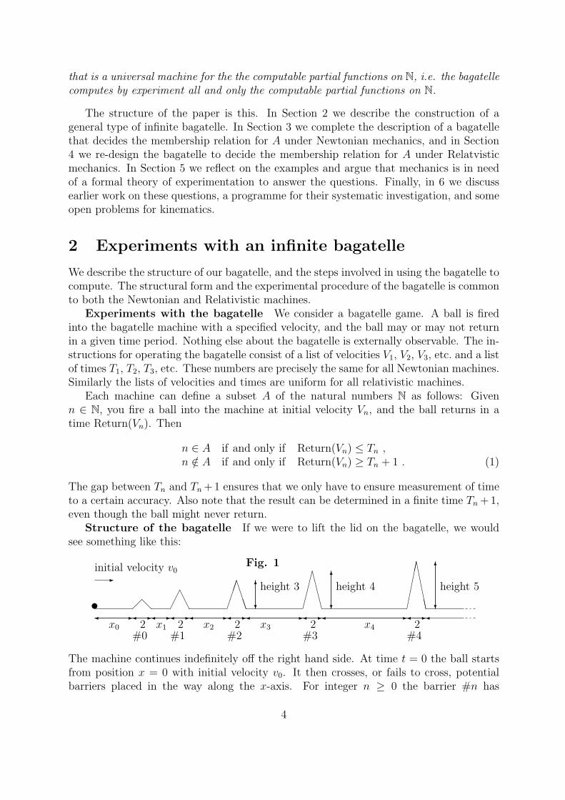
Structure of the bagatelle If we were to lift the lid on the bagatelle, we wouldsee something like this:

-initial velocity v0

u-�

x0

�@

#0

-�2

-�x1

��A

A

#1

-�2

-�x2

����B

BBB

#2

-�2

-�x3

����CCCC

#3

-�2

-�x4

������DDDDDD

#4

-�2

�

6

?

height 56

?

height 46

?

height 3

Fig. 1

The machine continues indefinitely off the right hand side. At time t = 0 the ball startsfrom position x = 0 with initial velocity v0. It then crosses, or fails to cross, potentialbarriers placed in the way along the x-axis. For integer n ≥ 0 the barrier #n has

4

height n + 1 and width 2. For simplicity we assume that it is has the shape of an isocelestriangle. The reader who is anxious about the sharp corners should compute the arbitarilysmall corrections in the formulae given by introducing arbitrarily small smoothings of thecorners. There is a flat gap (at height 0) between #n and #n+1 of length xn+1. We willgive the value of the numbers xn later.

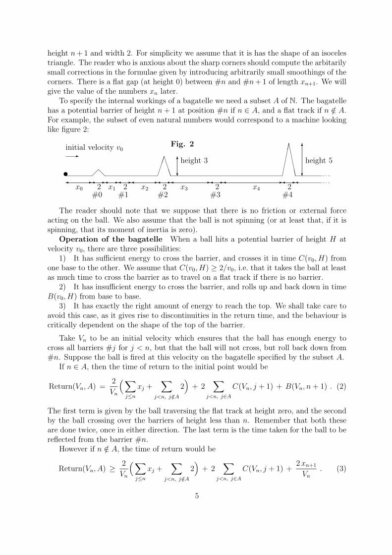
To specify the internal workings of a bagatelle we need a subset A of N. The bagatellehas a potential barrier of height n + 1 at position #n if n ∈ A, and a flat track if n /∈ A.For example, the subset of even natural numbers would correspond to a machine lookinglike figure 2:

-initial velocity v0

u-�

x0

�@

#0

-�2

-�x1

#1

-�2

-�x2

����B

BBB

#2

-�2

-�x3

#3

-�2

-�x4

������DDDDDD

#4

-�2

�

6

?

height 56

?

height 3

Fig. 2

The reader should note that we suppose that there is no friction or external forceacting on the ball. We also assume that the ball is not spinning (or at least that, if it isspinning, that its moment of inertia is zero).

Operation of the bagatelle When a ball hits a potential barrier of height H atvelocity v0, there are three possibilities:

1) It has sufficient energy to cross the barrier, and crosses it in time C(v0, H) fromone base to the other. We assume that C(v0, H) ≥ 2/v0, i.e. that it takes the ball at leastas much time to cross the barrier as to travel on a flat track if there is no barrier.

2) It has insufficient energy to cross the barrier, and rolls up and back down in timeB(v0, H) from base to base.

3) It has exactly the right amount of energy to reach the top. We shall take care toavoid this case, as it gives rise to discontinuities in the return time, and the behaviour iscritically dependent on the shape of the top of the barrier.

Take Vn to be an initial velocity which ensures that the ball has enough energy tocross all barriers #j for j < n, but that the ball will not cross, but roll back down from#n. Suppose the ball is fired at this velocity on the bagatelle specified by the subset A.

If n ∈ A, then the time of return to the initial point would be

Return(Vn, A) =2

Vn

( ∑j≤n

xj +∑

j<n, j /∈A

2)

+ 2∑

j<n, j∈A

C(Vn, j + 1) + B(Vn, n + 1) . (2)

The first term is given by the ball traversing the flat track at height zero, and the secondby the ball crossing over the barriers of height less than n. Remember that both theseare done twice, once in either direction. The last term is the time taken for the ball to bereflected from the barrier #n.

However if n /∈ A, the time of return would be

Return(Vn, A) ≥ 2

Vn

( ∑j≤n

xj +∑

j<n, j /∈A

2)

+ 2∑

j<n, j∈A

C(Vn, j + 1) +2 xn+1

Vn

. (3)

5

This time is based on the fact that if the ball did return, it would have to travel twiceover a flat track of length xn+1. Of course the ball might never return, as there might beno more barriers for it to cross, but this case is included in the inequality.

Choice of the displacements xn We want an experiment to determine if n ∈ A,and do not want the result confused by other elements of A. However our results (2) and(3) depend on elements in A which are less than n. We deal with this by considering thevalues taken as we vary A, and choose xn and Tn to be independent of A: First we choosethe sequence xn ≥ 0 satisfying the inequalities

xn+1 ≥∑j<n

(Vn C(Vn, j + 1)− 2

)+

Vn(B(Vn, n + 1) + 1)

2. (4)

Definition of the time bounds Tn Then we set Tn by

Tn =2

Vn

∑j≤n

xj + 2∑j<n

C(Vn, j + 1) + B(Vn, n + 1) . (5)

If n ∈ A, remembering that C(v0, H) ≥ 2/v0 we have from (2):

Return(Vn, A) ≤ 2

Vn

∑j≤n

xj + 2∑j<n

C(Vn, j + 1) + B(Vn, n + 1) = Tn. (6)

Correspondingly for n /∈ A, from (3) we have

Return(Vn, A) ≥ 2

Vn

( ∑j≤n

xj +∑j<n

2)

+2 xn+1

Vn

≥ Tn + 1 . (7)

It remains to find formulae for Vn, B and C in the Newtonian and relativistic cases.

3 Newtonian kinematics

The initial kinetic energy of the ball of mass m with any initial velocity v0 is 12mv2

0. Thepotential energy of the ball at height h above the initial point is mgh, where g is theacceleration due to gravity (on the Earth’s surface, this is about 9 ·8 meters/second2).The principle of conservation of energy then gives the velocity v of the ball at a height husing 1

2mv2

0 = 12mv2 + mgh. It follows that the maximum height H that the ball can

attain is given by 12mv2

0 = mgH, i.e. H = 12v2

0/g. We set Vn to be the initial velocity forwhich the maximum attainable height is n + 1

2, i.e.

Vn =√

g(2n + 1) . (8)

Proposition 3.1. The time taken for a ball with initial velocity v0 to climb a slope ofgradient n to a height h (less than the maximum height 1

2v2

0/g) is

v0 −√

v20 − 2gh

g

√1 +

1

n2.

6

Proof. We start the slope at the point (x, y) = (0, 0), so the equation of the slope isy = nx. On rearranging the conservation of energy equation, we see that at height ythe particle has velocity v =

√v2

0 − 2gy. The length of slope from height y to y + dy

is given by Pythagoras’ theorem as√

(dx)2 + (dy)2, or using the equation y = nx, as

dy√

1 + n2/n. The time taken to move from height y to y + dy is the distance dividedby the velocity, or dy

√1 + n2/(nv). This gives the total time to climb to height h as the

integral ∫ h

y=0

dy√

1 + n2

n√

v20 − 2gy

=v0 −

√v2

0 − 2gh

g

√1 +

1

n2. �

Corollary 3.2. The time taken for a ball with initial velocity v0 to climb a slope ofgradient n to its maximum attainable height is

v0

g

√1 +

1

n2.

Corollary 3.3. Using the definition of Vn in (8), we have, for j ≤ n,

C(Vn, j) = 2

√2n + 1−

√2n− 2j + 1

√g

√1 +

1

j2,

B(Vn, n + 1) = 2

√2n + 1√

g

√1 +

1

(n + 1)2.

Proof. We use the formulae given in 3.1 and 3.2, remembering that it takes the same timeto roll down as to climb up. �

Remark 3.4. Here we calculate asymptotic bounds on the time taken by the Newtonianbagatelle to decide if n ∈ A or not. From (8) and 3.3 we see that Vn, C(Vn, j) andB(Vn, n + 1) are all O(

√n). From (4) we can choose xn to be O(n2), and from (5) we

have Tn to be O(n5/2).

4 Relativistic kinematics

The relativistic mass of a ball of rest mass m travelling at velocity v is M = m/√

1− v2/c2,where c is the speed of light. The momentum of the ball is Mv, and we use the usualformula that force is the rate of change of momentum. On a slope inclined at an angleα to the horizontal, we have d

dt(Mv) = −Mg sin(α). On rearranging and differentiating

this yields dvdt

= −g(c2 − v2) sin(α)/c2. On integrating we get

v = c tanh(g(b− t) sin(α)/c) , (9)

where b is a constant. The initial velocity is

v0 = c tanh(gb sin(α)/c) , (10)

which, using a hyperbolic trig identity, becomes the useful formula

cosh(gb sin(α)/c) = 1/√

1− v20/c

2 . (11)

7

The distance travelled along the slope as a function of time is given by integrating (9)

d =c2

g sin(α)log

( cosh(bg sin(α)/c)

cosh((b− t)g sin(α)/c)

),

so the height as a function of time is

h =c2

glog

( cosh(bg sin(α)/c)

cosh((b− t)g sin(α)/c)

). (12)

The maximum height achieveable occurs when t = b, and is

hmax =c2

glog

(cosh(bg sin(α)/c)

). (13)

If the maximum height is set to n + 12, then using (11) and (13) the corresponding initial

velocity Vn is given by

Vn = c√

1− e−(2n+1)g/c2 . (14)

Proposition 4.1. The time taken for a ball with initial velocity v0 to climb a slope ofgradient sin α to a height h (less than the maximum height) is

c

g sin α

(tanh−1

(v0

c

)− cosh−1

( e−gh/c2√1− v2

0/c2

)).

Proof. If we rearrange (12) we get

cosh((b− t)g sin(α)/c) = cosh(bg sin(α)/c) e−gh/c2 ,

so we get t as

t = b− c

g sin αcosh−1

(cosh(bg sin(α)/c) e−gh/c2

). �

Corollary 4.2. The time taken for a ball with initial velocity v0 to climb a slope ofgradient sin α to its maximum attainable height is

c

g sin αtanh−1

(v0

c

).

Corollary 4.3. Using the definition of Vn in (14), we have, for j ≤ n,

C(Vn, j) =2 c

√1 + j2

g j

(cosh−1

(e(2n+1)g/(2c2)

)− cosh−1

(e(2n+1−2j)g/(2c2)

)),

B(Vn, n + 1) =2 c

√1 + (n + 1)2

g (n + 1)cosh−1

(e(2n+1)g/(2c2)

).

Proof. We use 4.1 and 4.2, with (11) and (14) supplying the formula

cosh(bg sin(α)/c) = e(2n+1)g/(2c2) . �

Remark 4.4. Here we calculate asymptotic bounds on the time taken by the relativisticbagatelle to decide if n ∈ A or not. From 4.3 we see that C(Vn, j) and B(Vn, n + 1) areboth O(n). For n large, Vn

∼= c. From (4) we can choose xn to be O(n2), and from (5) wehave Tn to be O(n3).

8

5 Commentary on the Bagatelle

5.1 Corollaries

Corollary 5.1. Any function f : N → N can be computed by a Newtonian or Relativisticbagatelle

Proof. Let Gf be the graph of f . Choose an injective function c : N2 → N such as(x, y) 7→ 2x.3y and code the graph Gf as the set c(Gf ). A bagatelle BA based on A = c(Gf )would enable f to be computed experimentally by the mechanical system.

Corollary 5.2. There exist Newtonian and Relativistic bagatelles that are universal ma-chines for the computable partial functions on N, i.e. the bagatelles compute by experimentall and only the computable partial functions on N.

Proof. Choose a bagatelle BA based on A = c(GU), the coded graph of a universal par-tial recursive function U . This would enable U to be computed experimentally by themechanical system.

5.2 Interpretations

All the bagatelles are systems that are valid in theoretical mechanics. Clearly, the struc-ture of the bagatelle BA is based on the set A and there is nothing in mechanics thatprevents or cautions us from defining such systems for any set A; thus, the bagatelle BA

is a legal mechanical system.Now, given any bagatelle BA then all the experiments needed to decide n ∈ A can be

carried out using the following primitive experimental actions :(i) project a particle with arbitrary large energy (for arbitrary large natural numbers);(ii) observe a fixed point in space;(iii) measure arbitrarily large times on a clock; and(iv) calculate with simple algebraic formulae.Indeed, the actions required are very simple and uncontentious. Thus, we have the

extreme and worrying result that valid or legal Newtonian and relativistic systems existto compute any set or function on N.

We call this the classical interpretation of the theorems because this is the standardway of interpreting theorems in classical mechanics. In particular, the existence of thebagatelle is proved using classical reasoning.

However, suppose the account of the experiment is required to explain how the me-chanical system is constructed, as well as what primitive experimental actions are neededto set initial states and observe behaviour. Then we find we have an interesting problem.

What assumptions underly our idea of an experiment with the bagatelle?Extending the informal ideas of Geroch and Hartle [22] on experiments designed to

measure quantities (see Section 6.2), then the experiments needed involve primitive ex-perimental actions of the following kind:

(i) selection steps from a source of unlimited natural resources;(ii) primitive construction steps (e.g., make a barrier and place a barrier);(iii) primitive experimental steps (e.g., project the particle, measure time);

9

(iv) schedule the three kinds of primitive steps, which may be interleaved, accordingto a global laboratory clock

With these actions we can postulate a precise form for an experiment:“Definition” An experiment is a finite or infinite process made of primitive construc-

tion or experimental steps indexed by the laboratory clock.Now, set against this definition of an experiment, one problem is that the sequence of

primitive steps in the construction of the system BA will involve knowledge of the set A -probably precisely the knowledge the system BA is being designed to reveal, making thepurpose of the experiment redundant. Since we are interested in the nature and use ofmechanical systems, this point about redundancy is not so interesting. What conditionswill be required on A to allow experiments on BA that are valid in this extended sense?An experiment could run as follows.

Suppose A is given by some increasing enumeration A0, A1, A2, . . . of finite subsetswith for each i ∈ N, Ai ⊂ Ai+1 and A =

⋃i∈N Ai. Suppose that Ai has i elements of A.

Then to make an experiment to decide if n ∈ A then we need an experimental procedureto construct a finite part of the bagatelle. This finite part will have the form BAk

for someAk ⊂ A. It will have k potential barriers located by the k elements of Ak.

An indepenedent laboratory clock will schedule the construction of the approximatingbagatelle BAk

and an experiment to decide n ∈ Ak. If the experiment confirms thatn ∈ Ak then we know that n ∈ A.

However, if the experiment confirms that n /∈ Ak then we do not know that n /∈ A.This result can change as k increases and more and more elements of A appear and thebagatelle grows. Each negative result must be repeated and so the experiment becomesa search for a positive result, secure in the knowledge that if n ∈ A then an experimentwith some part BAk

of the bagatelle BA will find it.Thus, when we include the construction of the bagatelle in the primitive steps we

have a proof that A is decidable by experiment if, and only if, finite subsets of A canbe generated by experiment. Indeed, we are close to a proof that A is decidable byexperiment if, and only if, A is recursively enumerable subset of N.

We call this the constructive interpretation of the theorems because we are addingprinciples of system construction to experimental principles of classical mechanics. Inparticular, the existence of the bagatelle is here proved using constructive reasoning.

6 Computable and non-computable physical systems

The general questions on computing with physical systems posed in the Introduction, andeven the special cases for particular kinds of physical system, are difficult problems. Toanswer them, physical theories must be combined with computability theories, and a clearaccount of the conduct of idealised experiments is necessary. Gedanken experiments havebe used since Galileo and are a complex philosophical subject in their own right, of course(see, e.g., Brown [12], Bohr [9], Koyre [27], Kuhn [30]). To cite an example in kinematics,gedanken experiments related to Zeno’s paradoxes have re-surfaced in philosopical debatesabout infinite machines and Newtonian supertasks (Perez Laraudogoitia [37, 38] and Alperand Bridger [3]).

10

Attempts to answer the questions often involve computable functions on continuousdata. Computation on continuous data can use algorithms that approximate infinite dataand so the concept consists of three ideas:

Computation = Data + Programs + Approximation.

There are many ways to model each of these three ideas. For example, data can be ab-stractly specified or concretely represented, programs can made from many different con-structs, and approximation can be expressed via orderings, norms, metrics and topologies.We do not yet possess a well understood theory of algorithmic computation for infinitedata, even on Rn. However, in the main computability theories on infinite data one findsthat if f is computable then f maps computable data to computable data. Therefore, inthe search for non-computability, it is common to seek systems that define a function fby experiment such that f returns non-computable output from computable input, sincesuch an f cannot be computable.

With these difficulties in mind, we consider some different approaches to the problemsby surveying representative work. This provides a landscape against which to appreciatethe study of mechanical examples of the kind given here.

6.1 The search for non-computability

The question “Is physical behaviour computable?” was asked in computability theory in,e.g., Kreisel [28]. The problem is unresolved, it will not go away, and has become moreconfusing, difficult and fascinating (Cooper and Odifreddi [14]).

Wave mechanics A major attempt at an answer was by Pour El and Richards, whoproposed “No”. In Pour El and Richards [42] they showed that there are solutions of the 3-dimensional wave equation with computable initial values that are are not computable overunit time [0, 1]. The notion of computable was based on the uniform norm on C[R3, R].The mathematical fact was later analysed in terms of the computability of operatorson Banach spaces in Pour El and Richards [44], and in the general setting of partialhomomorphisms of arbitrary metric partial algebras in Stoltenberg-Hansen and Tucker[57]. Because the wave equation is a fundamental model of physical phenomena, Pour Eland Richards suggested that the result indicated that there exist physical systems thatcould show non-computable behaviour. However, the experimental basis of the proposalwas too weak to support the suggestion, as pointed out in Kreisel [29].

Recently, Weihrauch and Zhong [65] have re-visited the wave equation, claiming thatby using the appropriate norms, solving the wave equation is a computable problem.They have shown that using the C1 norm on the differentiable functions C1[R3, R] (withuniform convergence of both the functions and their partial derivatives) and the uniformnorm on the continuous functions C[R3, R], that the wave equation solution operatorS ′ : C1[R3, R]×C[R3, R]×R → C[R3, R] is computable. Here S ′(f, g, t) is the solution tothe wave equation at time t which takes the value f at time zero and has velocity g at timezero. If the same type of norms are desired in both the initial and final conditions, theyalso showed that for all real numbers s and computable times t that S ′(t) : Hs[R3, R] ×Hs−1[R3, R] → Hs[R3, R] × Hs−1[R3, R] was computable, where Hs is a Sobolev space

11

of functions. Hence they propose that the answer is, in fact, “Yes” in the case of n-dimensional wave systems. In Weihrauch and Zhong [66] is a proof that the Schrodingerequation has computable solutions.

Let us try to convert the Pour El and Richards method to a ‘real’ experiment. We startwith a flat sheet of ice, and use a computer controlled tool to shape the surface. Thenwe instantaneously melt the ice, and the wave equation takes over. After a certain timewe make a measurement of the wave, and a ‘noncomputable’ result emerges. The toolshapes the surface according to a computable function, whose derivative is not computable(Myhill [35]). By a computable function, we mean that its value at a given point can becalculated to a given precision given enough time (i.e. clock cycles). If we insist thatthe construction be performed in a finite number of clock cycles, we could shape thesurface to, say, one micron of the theoretical function. But the uniform convergenceof functions does not imply convergence of the derivatives, as previously noted. In otherwords we cannot ensure that the derivative is anything like the theoretical value in a finitetime, so the result of any such experiment is likely to deviate widely from the calculated(noncomputable) result. The only way to achieve the theoretical result would be to havea ‘deus ex machina’ give the experimenters a precisely shaped ice sheet to begin with.This is just the situation which occurs with the bagatelle. To make one from a sheet ofmetal with a computer controlled tool, we either settle for a computable set of barriers,or we have to wait an infinite amount of time for the construction (and for many subsetseven an infinite amount of time will not do). In other words, the bagatelle throws up thesame philosophical points as the Pour El and Richards method, but does so in a moreobvious fashion.

Physical simulations of Turing machines To define a physical system that cansimulate a Turing machine one has to define the system, describe its operation and showhow an experiment with the system mimics the behaviour of a Turing machine. A soundargument should lead to the claim that the system can realise or implement all computablebehaviour and is a technology for digital computation. It may also yield results aboutnon-computable behaviour of the physical system from the undecidability of the haltingproblem for Turing machines.

A good example of this approach is Moore [33] on the “unpredictability” of physicalsystems. Moore shows how to model a Turing machine by a shift map, and, in turn,suggests a kinematic system, with a single particle guided by pin-ball “mirrors” in a3D potential, that is “equivalent” to a Turing machine. He argues that a Gedankenexperiment with a system corresponding with a universal Turing machine would haveundecidable behaviour. The motivation of the investigation is to show that such a systemis far more unpredicable than the common or garden chaoic system. Moore’s argumentsare suggestive rather than rigorous so, strictly speaking, the result is a conjecture.

Implementing Moore’s system in some idealised mechanics is quite interesting. Tomodel a Turing machine, the successive reflections have to be done with complete accuracy,any deviation will be magnified by successive reflections. In our idealised world we mayassume that light has no discernable wave nature, and will not diffract when passingthrough the system. However we also have to assume that the mirrors are perfectlyflat and perfectly positioned, which means that they cannot be made of atoms as weknow them. Such a rejection of the atomic hypothesis can easily lead to other strange

12

constructions, such as successive mechanical models of Turing machines, each half thesize of the last, and each doing its calculation in half the time of the last. If these wereconnected to perform successive steps of a calculation, infinitely many clock cycles couldbe performed in finite time.

Suggestions for simulating digital logic by kinematics are in Fredkin and Toffoli [20]Analogue computers Analogue computation as conceived by Lord Kelvin [58], V

Bush [13], and D Hartree [24], is experimental computation. The functions are of the formf : Rn → Rm and the physical systems are made from mechanical or electro-mechanicalcomponents. The theory of analogue computers is modest. A general purpose analogcomputer (GPAC) was introduced in Shannon [48] as a model of the Differential Analyserof Bush [13]. Shannon discovered that a function can be generated by a GPAC if, andonly if, it is differentially algebraic, but his proof was incomplete. An analysis in PourEl [40] yielded a new stronger model and a new proof of the equivalence (and somenew gaps corrected in Lipshitz and Rubel [31]). Using the characterisation in terms ofalgebraic differential equations, these analogue models were shown not to compute allcomputable functions on R (Pour El [40]). These models are close to the practice ofanalogue computing until the 1960s. That an undecidable predicate of a computablefunction on R might be experimentally computable by a suitable analogue machine wasobserved in Scarpellini [47].

Recently, the theory of analogue computing has been restarted by C Moore with verygeneral mathematical models (Moore [34]). These models define functions by schemesrather like Kleene’s, but with primitive recursion replaced by integration and others added,but can define functions beyond the class of computable functions on R. In Graca andCosta [23] another model close to the GPAC has been shown to be equivalent with asubclass of Moore’s functions (those defined by composition and integration).

Neural networks Among the first attempts to model physical systems as computingdevices is McCulloch and Pitts logical models of networks of neurones. Neural networkshave been influential in digital computing (e.g., von Neumann’s abstraction of computerarchitecture, Kleene’s regular expressions, parallelism). They have also involved the in-terface between discrete and continuous notions.

The theory of neural networks is vast. The McCulloch and Pitts proposal that neuraltissue can be modelled as hybrid logical/algorithmic networks has led to many resultsthat confirm that the answer to the question ”Are neural systems computable?” is “Yes”(e.g., see Holden et al [25]). However, a convenient survey of models and a proposal thatsome hybrid nets are not is in Siegelmann [52]. From the point of view of a theory ofexperimental computation, the arguments for this negative answer are not adequate, asthe analysis in Davis [17] demonstrates. The strong debate of Penrose’s proposals in [39]is also a rejection of the positive answer.

Quantum computing The experimental nature of computation, which our kinematiccomputers illuminate, is also the basis of the more complex field of quantum computation.Informal notions of quantum algorithms, computers and circuits have been developed andthe the physical aspects of the Church-Turing Thesis discussed since Benioff [6], Deutsch[18, 19] and Yao [67]. Comparisons with classical computation have been focussed onthe superior speed of quantum computation. An early rigorous definition of a quantumTuring machine is in Bernstein and Vazirani [7] where it is shown that the quantum

13

Turing machine can be simulated by a classical one and vice versa. However, the for-mulation of some quantum computer models rely on classical computability theory sincethey are require certain real number parameters must be computable. For example, in[7] probability amplitudes associated with state transitions are assumed computable oreven rational; this hypothesis is relaxed in Adleman, DeMarrais, and Huang [2]. In somecases, quantum models are presented as a computable family of circuits. The justificationof such extra hypotheses in experimental terms is an interesting problem. Many modelsfor quantum computation are being developed and our understanding of this complexnotion of computation is at an early stage. It seems not to be known if quantum cellularautomata (Margolus [32]) can be simulated by a classical Turing machine.

Classical versus quantum systems Penrose’s study and reflections on computabil-ity, physical laws and consciousness have stimulated a great deal of thought about thecomputability of physical systems and the mind (Penrose [39]). Relevant here is his con-jecture that nature can produce non-computable processes that we can use but not at thelevel of classical physics. In da Costa and Doria [16] this idea is formulated as Penrose’sThesis and a “counter-example” suggested, based on da Costa and Doria [15], that showsclassical mechanics can produce non-computable behaviour. We consider the counter-example is not convincing, not least because it complicated and fails to allow a robustexperiment. Our bagatelle shows that the simplest examples of classical mechanics cer-tainly allow non-computable behaviour but it is the notion of experiment that determineswhat can or cannot be harnessed.

Noncomputablility in dynamical systems There are several general classes ofmathematical system that have their origins as classes of physical model, and aboutwhich computability results have been proved. These results simulate models such asTuring machines by ODEs or cellular automata, or encode undecidable problems in decisonproblems for dynamical systems. They are interesting because they suggest avenues fordevising new idealised experiments with physical systems and are destined to belong to atheory framework. However, as mathematical systems, they have abstracted away fromhow physical ideas can be use to perform computation. Some examples follow. Theexistence of an ODE with computable initial conditions and no computable solution isproved in Pour El and Richards [41]. The simulation of machines by ODEs has been shownfor finite automata in Brockett [11], and for Turing machines in Branicky [10]. Decisionproblems for the differential equations of mechanics are not new. An early problem in thequalititaive theory of celestial mechanics is Poincare’s Centre Problem (see, e.g., Seigeland Moser [51]). A recent example of undecidability is da Costa and Doria [15] on theintegration of Hamiltonians using quadratures, proved using the undecidability of theintegration of elementary functions (Richardson [45]).

6.2 The search for a conceptual analysis

The search for non-computable aspects of particular physical examples, or of whole classesof mathematical models, must be complemented by a search for the general concepts andprinciples that enable physical systems to be used for computing. The aim is to findconcepts, axioms and laws that can (a) embrace diverse examples of physical systemsthat may be said to compute; (b) explore the border between computability and non-

14

computability; and (c) facilitate comparisons with general classes of mathematical modelsof physical systems and computers.

First, we might isolate the essential properties of(i) experimentation, which are focussed on obtaining input and output, and(ii) behaviour, which are focussed by the operation of a system.We have sketched some simple ideas about experimentation in Section 5, enough to

set up and criticise our bagatelles. A fuller analysis of experimentation would study theprocesses of observation, measurement and construction of a system, which are intercon-nected and dependent on some underlying theory for the system. In Geroch and Hartle[22], there is an attempt at characterising the numerical quantities that are measurable byexperiment. We extended their conditions for experiments in Section 5. They argue thatany number computable by algorithms is measurable by experiment because the process ofapplying an algorithm qualifies as an idealised experiment. Conversely, they argue thatthese measurable quantities are also computable numbers, at least when experiments arebased on “conventional” physical theories. They ask if quantum gravity is a theory wherethis may fail. Although stimulating, their ideas about experiments fall short of axiomaticanalysis.

A formal general property of experiments is the continuity of the input-output rela-tion. The idea being that in performing meaningful experiments the results must displaysome robustness when they are repeated with small changes in initial and conditions andobservable behaviour. This property is proposed in Kreisel [28], where the idea is referedto as Hadamard’s Principle for well-posed systems. Continuity is also the key idea in thegeneral mathematical arguments of Weihrauch and Zhong [65]. If continuity is a necessarycharacteristic of the function computed by an experiment then it is worth noting that ondata types with metric space structures Ceitin’s Theorem says, roughly, that computablityimplies continuity. Studies of generalisations and converses of this theorem are Spreen[53] and Stoltenberg-Hansen and Tucker [57].

Thus, in designing physical systems for computation, one proviso is to avoid singularcases which give rise to discontinuities. In the mechanics of point particles, in the case ofscattering off a barrier with a sharp corner, there is a singular case when a particle hitsthe vertex of the angle of the corner. In the case of the gravitational dynamics of pointparticles, a singular case arises when point particles collide. In the bagatelle we mustchoose input velocities that avoid the singular behaviour of a ball coming to rest at thetop of a potential barrier.

However, to answer the questions, we seek sets of basic axioms that such an idealisedphysical system might satisfy if we are to use it in idealised experiments for computation.Our idea is to restrict attention to axiomatising the information processing capabilities ofsystems in which the behaviour of the physical system is based on a “finite” transformation,propagation and observation of material, energy, or information. In Beggs and Tucker [4]we give axioms for the local structures of systems and their local states.

An attempt at such an axiomatistion of machines for digital processing is Gandy [21]in which notions of space and causality are modelled using hereditarily finite sets. Theconceptual analysis is frustratingly difficult to use and has been studied in some depth bySieg [49, 50]. This analysis, although focussed on refining the idea of mechanical compu-tation as portayed in Turing machines, is relevant to our problem. Digital computation

15

by machines is also an example of physical computation and should properly fall withinthe scope of the problem. Digital computation is based on software and hardware systemsthat must be described both by abstract programs and machine architectures obeying thelaws of logic, and by systems obeying the laws of physics. Our own axiomatisation owessomething to Gandy’s, though it is shaped by the study of computing with the systemsof classical mechanics.

6.3 Concluding remarks on kinematic systems

In conclusion, experimental computation is not well understood and the questions askedin the introduction are open, even in the case of kinematics, possibly the simplest physicaltheory. There is a paucity of examples that can be formulated and studied in completedetail, though plenty of informal ideas and speculations have been aired. Classical me-chanical systems offer interesting problems and insights into experimental computation.

Our result about arbitrary subsets A ⊂ N is new. Most attempts at undecidabilityembed recursively enumerable but non-recursive sets into models of physical systems, e.g.,by simulating Turing machines and examining their halting problem. The fact that anysubset of the natural numbers can be recognised by a simple mechanical system raises analarm because the theory of the subsets of natural numbers is so vastly complicated itdepends on the foundations of set theory for its exploration. Let us note that many setsof computational interest lie in the arithmetic hierarchy, which is a countable family ofsubsets of the natural numbers that already contains sets that are in a convincing senseinfinitely more undecidable than the halting problem (see Rogers [46]).

Our bagatelles are systems that each require unbounded space, time and energy todecide n ∈ A for all n ∈ N. Consider energy. In each of our Newtonian bagatelles massis bounded (indeed, it can be an arbitrary constant) and velocity is unbounded. In eachof our Relativistic bagatelles velocity is bounded and mass is unbounded. One can ask ifthere are examples of kinematic systems that are bounded in space, time and energy?

In Newtonian mechanics we are allowed to shrink space and accelerate time. Forexample, the natural numbers n = 0, 1, 2, . . . that mark points in space or steps in timecan be embedded into the interval [0, 1] by n 7→ 1/2n. Shrinking space leads to mechanicalsystems that use arbitrarily small components. Of course, a mechanical system thatexploits the infinite divisibility of space, with no lower bounds on units of space and time,violates any form of atomic theory. But such examples are sharp tools to investigate thetheoretical foundations of computability and mechanics. In fact, it is possible to provethat for each set A ⊂ N there exists a valid Newtonian kinematic system SA, which isembedded within a bounded 3-dimensional box, operates entirely within a fixed finitetime interval using a fixed finite amount of energy, and can decide the membership of thesubset A (Beggs and Tucker [5]).

However, an open problem is this:

Problem 6.1. For all valid kinematic systems that possess both lower and upper boundson space, time, mass, velocity and energy, are the sets and functions computable by ex-periment also computable by algorithms?

We conjecture that the answer is “Yes”. To prove this, one needs axiomatisations of

16

the kind discussed in Section 6.2.Our bagatelle examples show that the notion of mechanical system - i.e., what qualifies

as a valid or legal system in theoretical mechanics - must be sharpened. To the standardparameters of mass, velocity, distance, time we need to add formal theory that constrainsthe structure and construction of the system and explains how experiments are performed.

Theoretical intuitions about making experiments turn out to be strikingly similar tointuitions about algorithms and computers, although the primitive actions are differentand are implicit in the physical theory. Indeed, we conjecture that a theory of Gedankenexperiments for mechanics, if formalised, could be capable of underpinning the theory ofthe computable as follows:

Problem 6.2. Extend theoretical mechanics by a mathematical theory of construction andobservation of mechanical systems, and show that the sets and functions computable byexperiment are precisely those computable by algorithms.

One goal of this direction of research, from physical theory to computablity, is, roughlyspeaking, To derive forms of Church-Turing Thesis as physical laws.

The bagatelle theorem is a theorem based on classical mathematical reasoning. It re-veals the necessity of making explicit the nature of experiments in mechanical theorems.From the point of view of mathematical logic and computability theory, mechanical sys-tems need specification languages that can describe formally their physical structure,construction and observation. However, from the point of view of philosophical founda-tions, we can reject classical mathematical reasoning, which allows the construction ofsuch omnipotent mechanical systems, and use constructive mathematical reasoning. Hereis another problem:

Problem 6.3. Develop a constructive theoretical mechanics, based on constructive math-ematical reasoning, in which experiments are part of the basis for mathematical existence.

Finally, we should raise the special case of efficient computation by mechanical sys-tems. New theory is needed to pose and answer a question such as:

Problem 6.4. Are there sets that can be decided in polynomially bounded space and timeby experimental computation with mechanical systems but cannot be decided by algorithmsin polynomial space and time?

We thank A V Holden, V Stoltenberg-Hansen, and J I Zucker for discussions on someof the areas mentioned in this paper, and the following for advice on literature: AnujDawar (quantum computation) and Brendan Larvor (Gedanken experiments).

References

[1] O Aberth, Computable Analysis, McGraw-Hill, New York, 1980.

[2] L M Adleman, J DeMarrais, M-D A Huang, Quantum Computability, SIAMJournal of Computing, 26 (1997) 1524 - 1540.

[3] J Alper and M Bridger, Newtonian supertasks: A critical review, Synthese 114(1998), 355 – 369.

17

[4] E J Beggs and J V Tucker, Computations via experiments with physical sys-tems: some axioms and examples, in preparation.

[5] E J Beggs and J V Tucker, Newtonian systems, bounded in space, time andenergy can compute all functions, in preparation.

[6] P Benioff, The computer as a physical system: A microscopic quantum mechani-cal Hamiltonian model of computers as represented by Turing machines, Journal ofStatistical Physics, 22 (1980) 563-591.

[7] E Bernstein and U Vazirani, Quantum complexity theory, SIAM Journal ofComputing, 26 (1997) 1411 - 1473.

[8] L Blum, F Cucker, M Shub and S Smale, Complexity and Real Computation,Springer-Verlag, New York, 1998.

[9] N Bohr, Discussions with Einstein on epistemological problems in atomic physics,in P A Schillpp, Albert Einstein: Philosopher-Scientist, Open Court, La Salle, 1949.

[10] M S Branicky, Analog computation with continuous ODEs, in H L Trentelman andJ C Willems (eds), Essays in Control: Perspectives in the Theory and its Applications,Dallas Texas, IEEE, 1994, 265-274.

[11] R W Brockett, Hybrid models for motion control systems, in Proceedings IEEEWorkshop on Physics and Computation, Birkhauser, Boston, 1993, 29-53.

[12] J R Brown, The Laboratory of the Mind.: Thought Experiments in the NaturalSciences, Routledge, London, 1991.

[13] V Bush, The differential analyser. A new machine for solving differential equations,Journal of Franklin Institute 212 (1931), 447-488.

[14] S B Cooper and P Odifreddi, Incomputability in nature, in S. B. Cooper and S.S. Goncharov, (eds.), Computability and Models: Perspectives East and West, KluwerAcademic/Plenum Publishers, Dordrecht, 2003, pp. 137-160.

[15] N C A da Costa and F A Doria, Undecidability and incompleteness in classicalmechanics, International Journal of Theoretical Physics 30 (1991), 1041-1073.

[16] N C A da Costa and F A Doria, Classical physics and Penrose’s thesis, Foun-dations of Physics Letters 4 (1991), 363-373.

[17] M Davis, The myth of hypercomputation, in Turing Festschrift, Springer, in prepa-ration.

[18] D Deutsch, Quantum theory, the Church-Turing principle, and the universal quan-tum computer, Proceedings Royal Society London A 400 (1985), 97-117.

[19] D Deutsch, Quantum computational networks, Proceedings Royal Society LondonA 425 (1989), 73-??.

18

[20] E Fredkin and T Toffoli, Conservative logic, International Journal of Theoret-ical Physics 21 (1982), 219-253.

[21] R Gandy, Church’s thesis and principles for mechanism, in J Barwise, HJ Keisler,and K Kunen (eds.) The Kleene Symposium, North-Holland, 1980, pp.123–148.

[22] R Geroch and J B Hartle, Computability and physical theories, Foundationsof Physics 16 (1986), 533-550.

[23] D S Graca and J F Costa, Analog computers and recursive functions over thereals, 2003, submitted.

[24] D R Hartree, Calculating Instruments and Machines, Cambridge University Press,1950.

[25] A V Holden, J V Tucker, H Zhang and M Poole, Coupled map lattices ascomputational systems, American Institute of Physics - Chaos 2 (1992), 367-376.

[26] E Griffor, (ed) Handbook of Computability Theory, Elsevier, 1999.

[27] A Koyre, Galileo’s treatise De Motu: the use and abuse of imaginary experiment,in Metaphysics and Measurement, Chapman and Hall, London, 1968.

[28] G Kreisel, A notion of mechanistic theory, Synthese 29 (1974), 9-24.

[29] G Kreisel, Review of Pour El and Richards, Journal of Symbolic Logic 47 (1974),900-902.

[30] T S Kuhn, A function for thought experiments, in T S Kuhn, The Essential Tension,University of Chicago Press, Chicago, 1977.

[31] L Lipshitz and L A Rubel, A differentially algebraic replacement theorem, Pro-ceedings of the American Mathematical Society 99(2) (1987), 367 – 372.

[32] N Margolus, Parallel Quantum Computation, in W.H. Zurek (ed.), Complexity,Entropy, and the Physics of Information VIII, Addison-Wesley, 1990.

[33] C Moore, Unpredictability and undecidability in dynamical systems, Physical Re-view Letters 64 (1990), 2354 – 2357.

[34] C Moore, Recursion theory on the reals and continuous time computation, Theo-retical Computer Science 162 (1996), 23 – 44.

[35] J Myhill, A recursive function defined on a compact interval and having a contin-uous derivative that is not recursive, Michigan Mathematics Journal 18 (1971), 97 –98.

[36] P Odifreddi, Classical Recursion Theory, Studies in Logic and the Foundations ofmathematics, Vol 129, North-Holland, Amsterdam, 1989.

[37] J Perez Laraudogoitia, A beautiful supertask, Mind 105 (1996), 81 – 83.

19

[38] J Perez Laraudogoitia, Infinity machines and creation ex nihilo, Synthese 114(1998), 259 – 265.

[39] R Penrose, The Emperor’s New Mind, Oxford University Press, 1989.

[40] M B Pour-El, Abstract computability and its relations to the general purposeanalog computer, Transactions of the American Mathematical Society 199 (1974), 1– 28.

[41] M B Pour-El and J. I. Richards, A computable ordinary differential equationwhich possesses no computable solution, Annals of Mathematical Logic 17 (1979), 61– 90.

[42] M B Pour-El and J. I. Richards, The wave equation with computable initialdata such that its unique solution is not computable, Advances in Mathematics 39(1981), 215 – 239.

[43] M B Pour-El and J. I. Richards, Computability and noncomputability in clas-sical analysis, Transactions of the American Mathematical Society 275 (1983), 539 –560.

[44] M B Pour-El and J. I. Richards, Computability in Analysis and Physics, Per-spectives in Mathematical Logic, Springer-Verlag, Berlin, 1989.

[45] D Richardson, Some undecidable problems involving elementary functions of areal variable, Journal for Symbolic Logic 33 (1968), 514–520.

[46] H Rogers, Theory of recursive Functions and Effective Computability, McGraw-Hill, New York, 1967.

[47] B Scarpellini, Zwei Unentscheitbare Probleme der Analysis, Zeitschrift fur Math-ematische Logik und Grundlagen der Mathematik 9 (1963), 265-289.

[48] C Shannon, Mathematical theory of the differential analyser, Journal of Mathe-matics and Physics 20 (1941), 337-354.

[49] W Sieg, Calculations by man and machine: mathematical presentation, in P Gar-denfors, J Wolenski and K Kijania-Placek (eds.) In the Scope of Logic, Methodologyand Philosophy of Science. Volume I, Kluwer, 2002, pp.247–262.

[50] W Sieg, Calculations by man and machine: conceptual analysis, in W Sieg, RSommer and C Talcott (eds.) Reflections on the foundations of mathematics. Essaysin honor of Solomon Feferman, Association for Symbolic Logic, 2002, pp.390–409.

[51] C L Seigel and J K Moser, Lectures on Celestial Mechanics, Springer-Verlag,Berlin, 1971.

[52] H T Siegelmann, Neural networks and analog computation: Beyond the Turinglimit, Birkhauser, Boston, 1999.

20

[53] D Spreen, On effective topological spaces, Journal of Symbolic Logic 63 (1998),185-221.

[54] V Stoltenberg-Hansen and J V Tucker, Effective algebras, in S Abramsky,D Gabbay and T Maibaum (eds.) Handbook of Logic in Computer Science. VolumeIV: Semantic Modelling, Oxford University Press, 1995, pp.357-526.

[55] V Stoltenberg-Hansen and J V Tucker, Computable rings and fields, in E.R. Griffor (ed.), Handbook of Computability Theory, Elsevier, 1999, 363 – 447.

[56] V Stoltenberg-Hansen and J V Tucker, Concrete models of computation fortopological algebras, Theoretical Computer Science 219 (1999), 347 – 378.

[57] V Stoltenberg-Hansen and J V Tucker, Computable and continuous partialhomomorphisms on metric partial algebras, Bulletin for Symbolic Logic 9 (2003), 299– 334.

[58] W Thompson and P G Tait, Treatise on Natural Philosophy, Second Edition,Part I, Cambridge UniversityPress, 1880, Appendix B’, 479-508.

[59] J V Tucker and J I Zucker, Computation by while programs on topologicalpartial algebras, Theoretical Computer Science 219 (1999), 379 – 421.

[60] J V Tucker and J I Zucker, Computable functions and semicomputable sets onmany sorted algebras, in S. Abramsky, D. Gabbay and T Maibaum (eds.), Handbookof Logic for Computer Science volume V, Oxford University Press, 2000, 317 – 523.

[61] J V Tucker and J I Zucker, Abstract versus concrete computation on metricpartial algebras, ACM Transactions on Computational Logic, in press.

[62] K Weihrauch, Computable Analysis, An introduction, Springer-Verlag, Heidelberg,2000.

[63] K Weihrauch and U Schreiber, Embedding metric spaces into cpo’s, TheoreticalComputer Science 16 (1981), 5 – 24.

[64] K Weihrauch and N Zhong, The wave propagator is Turing computable, in JWiedermann, Peter van Emde Boas, and M Nielsen (editors), Automata, languagesand programming, 26th Colloquium, 1999, Springer Lecture Notes in Computer Sci-ence, volume 1644, Springer-Verlag, Berlin, 1999, 697 – 706.

[65] K Weihrauch and N Zhong, Is wave propogation computable or can wave com-puters beat the Turing machine?, Proceedings of London Mathematical Society 85(2002), 312-332.

[66] K Weihrauch and N Zhong, Is the Schrodinger propagator Turing computable?,in J. E. Blanck, V. Brattka and P. Hertling (eds.), Computability and complexity inAnalysis, Springer Lecture Notes in Computer Science, Volume 2064, 2001.

[67] A Yao, Quantum circuit complexity, Proceedings 34th Annual IEEE Symposium onFoundations of Computer Science, 1993, 352-361.

21