Embed Size (px)
Citation preview

Helsinki University of TechnologyLaboratory of Computational EngineeringEspoo 2006 REPORT B60
COMPUTATIONAL STUDIES OF SILICONINTERFACES AND AMORPHOUS SILICA
Sebastian von Alfthan
Dissertation for the degree of Doctor of Science in Technology to be presented with due permission ofthe Department of Electrical and Communications Engineering, Helsinki University of Technology, forpublic examination and debate in Auditorium N at Helsinki University of Technology (Espoo, Finland)on the 18th of December, 2006, at 12 noon.
Helsinki University of TechnologyDepartment of Electrical and Communications EngineeringLaboratory of Computational Engineering
Tekniska HögskolanAvdelningen för el och telekommunikationsteknikLaboratoriet för datorbaserad vetenskap och teknik
Teknillinen korkeakouluSähkö- ja tietoliikennetekniikan osastoLaskennallisen tekniikan laboratorio

Distribution:Helsinki University of TechnologyLaboratory of Computational EngineeringP. O. Box 9203FIN-02015 HUTFINLANDTel. +358-9-451 4845Fax. +358-9-451 4830http://www.lce.hut.fi
Online in PDF format: http://lib.tkk.fi/Diss/2006/isbn9512285401/
E-mail: [email protected]
c©Sebastian von Alfthan
ISBN-13 978-951-22-8539-6 (printed)ISBN-10 951-22-8539-8 (printed)ISBN-13 978-951-22-8540-2 (PDF)ISBN-10 951-22-8540-1 (Pdf)ISSN 1455-0474
Picaset OyHelsinki 2006

Abstract
Computational simulations are a new branch of science where one can performcomputational experiments by simulating a model system. The model contains anapproximation of a real system with simplified physical laws and reduced sizein order to make it computationally tractable. Many physical systems cannotbe analytically solved and also experimentally not everything can be measured.Computational simulations fill the gaps and allow new kinds of problems to beaddressed.
Two main issues are studied in this thesis with computational simulations. Thefirst issue concerns interfaces in silicon and is studied with deterministic molec-ular dynamics simulations. The second issue concerns the amorphous state ofsilicon and silica created with a stochastic algorithm.
As for the first issue the first study is a preliminary investigation of the heatconductivity over an amorphous-crystalline interface in silicon. Second, we presenta methodology for calculating the life-time of large amorphous clusters embed-ded in a crystalline matrix by simulating much smaller clusters. We employ thismethodology to study amorphous silicon clusters and find that the activation en-ergy of the boundary movement is temperature dependent with a change in behav-ior at 1150 K. The last problem concerns the structure of twist grain boundariesat 0 K. We present detailed simulations where we explore many possible grainboundary structures by allowing the number of atoms at the interface to change.This is a degree of freedom that has not been previously considered in computa-tional studies and proved to be of utmost importance. We find that the twist grainboundaries have ordered structures at 0 K for atomic densities at the interface notpreviously considered. We also find that the structural unit model is valid for twistgrain boundaries and present the structural units forming the boundary.
The second issue concerns the amorphous state of silicon and silica. With astochastic Monte Carlo simulation method that operates on the bond network ofsilicon and silica, we have created both amorphous silicon and silica. We findthat we can improve the structural description of amorhous silica by adjustingthe potential model. In addition, we developed optimizations for the simulationmethod which made it tractable for larger systems.

ii Abstract

Sammandrag
Simulationer utförda med datorer är en ny vetenskapsgren, där man kan genom-föra datorexperiment genom att simulera ett modellsystem. Modellen innehålleren approximation av ett verkligt system med förenklade fysikaliska lagar och för-minskad storlek. Många fysikaliska system kan inte lösas analytiskt, och ävenexperimentellt går det inte att mäta allting. Simulationer fyller i luckorna ochmöjliggör forskning inom nya områden.
Två huvudsakliga frågor har undersökts med simulationer i denna avhandling.Den första frågan gällande gränssnitt i kisel undersöks med hjälp av determinis-tiska molekylärdynamik-simulationer. Den andra frågan gäller det amorfa tillstån-det i kisel samt kiseldioxid, och undersöks med hjälp av en stokastisk algoritm.
Den första studien är en preliminär undersökning av värmeledningsförmågangenom ett gränssnitt mellan amorft och kristallint kisel. Den andra studien pre-senterar en metodologi med vilken man kan beräkna livslängden för stora amorfaklot inbyggda i en kristall genom att simulera små klot. Vi använder oss av dennametodologi för att studera amorfa kiselklot, och finner att gränssnittets rörlighethar en temperaturberoende aktiveringsenergi. Den sista studien i den första frågangäller den atomistiska strukturen av korngränser vid 0 K. Vi presenterar detaljer-ade simulationer, i vilka vi undersöker flera olika korngränsstrukturer genom attvariera mängden atomer vid kontaktytan. Detta är en frihetsgrad som inte hartidigare beaktats, och den visade sig vara mycket betydelsefull. Vi kommer framtill att korngränser har en ordnad struktur, samt att korngränser är uppbyggda avstrukturella enheter.
Den andra frågan gäller det amorfa tillståndet av kisel samt kiseldioxid. Vihar skapat amorft kisel och kiseldioxid med hjälp av en stokastisk Monte Carlo-metod som opererar på nätverket av atombindningar. Vi har kommit fram till attvi kan förbättra den strukturella beskrivningen av amorft kiseldioxid genom attmodifiera dess potentialmodell. Vi har även utvecklat en optimerad version avmetoden, vilket möjliggör simuleringar av större system.

iv Sammandrag

Preface
The research presented in this dissertation has been carried out at the Laboratoryof Computational Engineering at Helsinki University of Technology during theyears 2002-2006. First, I would like to thank Prof. Adrian Sutton for his guidance,and for being a great source of inspiration. His knowledge and ideas have beenof vital importance in my research. I would also like to express my gratitudeto Prof. Kimmo Kaski for support and for providing excellent facilities at thelaboratory. Dr. Antti Kuronen was of great help in the first part of this study.In addition, I would like to thank Fred Streitz and Jim Glosli for hosting me atLawrence Livermore National Laboratory in the summer of 2005, which was agreat experience both professionally and personally.
I am also thankfull to past and present colleagues and friends at the laboratory,especially Teemu Leppänen, Markus Miettinen, Petri Nikunen, Laura Kauhanen,Ilkka Kalliomäki, Toni Tamminen and Aapo Nummenmaa. In addition, I wouldlike to thank my family for getting me this far. Finally, I would like to thank Virpifor all the support she has given.
Sebastian von Alfthan

vi Preface
List of publications and author’scontributions
This dissertation consists of an overview and the following publications:
I. S. von Alfthan, A. Kuronen, K. Kaski, Crystalline-amorphous interface: molecu-lar dynamics simulation of thermal conductivity, Mater. Res. Soc. Symp. Proc.703, V6.2.1 (2002).
II. S. von Alfthan, A. Kuronen, K. Kaski, Realistic models of amorphous silica: Acomparative study of different potentials, Phys. Rev. B 68, 73203 (2003).
III. S. von Alfthan, A.P. Sutton, A. Kuronen, K. Kaski, Stability and crystallization ofamorphous clusters in crystalline Si, J. Phys.: Condens. Matter 17, 4263 (2005).
IV. S. von Alfthan, P.D. Haynes, K. Kaski, A.P. Sutton, Are the structures of twistgrain boundaries ordered at 0 K, Phys. Rev. Lett. 96, 55505 (2006).
V. S. von Alfthan, K. Kaski, A.P. Sutton, Order and structural units in simulations oftwist grain boundaries in silicon at absolute zero, Phys. Rev. B 74, 134101 (2006).
In the overview, these publications are referred to by their roman numerals. Theauthor has played an active and vital role in the research reported here. He has per-formed all computational simulations and written the simulation programs, withtwo exceptions: the molecular dynamics program used in Publications I and IIIand the DFT simulations in Publication IV. He has also analyzed the simulationdata and has developed all non-standard analysis tools. In addition, he has de-veloped a visualization software which has been used for figures in PublicationsIII-V. The author has written Publications II-V and has contributed to writing Pub-lication I.

viii Contents

Contents
Abstract i
Sammandrag iii
Preface v
List of publications and author’s contributions vii
Contents ix
1 Introduction 1
2 Interfaces and disorder in silicon and silica 32.1 Silicon . . . . . . . . . . . . . . . . . . . . . . . . . . . . . . . . 32.2 Silica . . . . . . . . . . . . . . . . . . . . . . . . . . . . . . . . 42.3 Amorphous state . . . . . . . . . . . . . . . . . . . . . . . . . . 52.4 Grain boundaries in silicon . . . . . . . . . . . . . . . . . . . . . 7
2.4.1 Geometry . . . . . . . . . . . . . . . . . . . . . . . . . . 72.4.2 Atomistic structure . . . . . . . . . . . . . . . . . . . . . 10
3 Computer simulations 133.1 Potential models . . . . . . . . . . . . . . . . . . . . . . . . . . . 13
3.1.1 Stillinger-Weber potential . . . . . . . . . . . . . . . . . 153.1.2 Tersoff potential . . . . . . . . . . . . . . . . . . . . . . 163.1.3 Modified Keating potential . . . . . . . . . . . . . . . . . 17
3.2 Molecular dynamics . . . . . . . . . . . . . . . . . . . . . . . . . 183.2.1 Algorithm . . . . . . . . . . . . . . . . . . . . . . . . . . 19

x Contents
3.2.2 Measured quantities . . . . . . . . . . . . . . . . . . . . 213.2.3 Force calculation . . . . . . . . . . . . . . . . . . . . . . 22
3.3 Monte Carlo . . . . . . . . . . . . . . . . . . . . . . . . . . . . . 223.3.1 Wooten, Winer and Weaire method . . . . . . . . . . . . 24
3.4 Minimization of atomistic systems . . . . . . . . . . . . . . . . . 273.4.1 Conjugate gradient method . . . . . . . . . . . . . . . . . 273.4.2 Simulated annealing . . . . . . . . . . . . . . . . . . . . 28
4 Analysis of simulation data 314.1 Radial distribution function . . . . . . . . . . . . . . . . . . . . . 314.2 Ring statistics . . . . . . . . . . . . . . . . . . . . . . . . . . . . 324.3 Structural order parameters . . . . . . . . . . . . . . . . . . . . . 32
4.3.1 Position dependent order parameter . . . . . . . . . . . . 334.3.2 Bond orientational order parameter . . . . . . . . . . . . 33
4.4 Visualization . . . . . . . . . . . . . . . . . . . . . . . . . . . . 35
5 Overview of the results 375.1 Heat transfer over an amorphous/crystalline interface in silicon . . 375.2 Improved potential model for amorphous silica . . . . . . . . . . 385.3 Stability of spherical amorphous clusters . . . . . . . . . . . . . . 395.4 Twist grain boundaries in silicon . . . . . . . . . . . . . . . . . . 40
5.4.1 Computational approach . . . . . . . . . . . . . . . . . . 405.4.2 Results . . . . . . . . . . . . . . . . . . . . . . . . . . . 41
6 Summary 47
A Atomicdx 49
References 53

Chapter 1
Introduction
In physics there has traditionally been two branches of research, theoretical andexperimental. Theories describe our understanding of the laws of nature, andexperiments attempt to measure physical phenomena. Theories are tested andverified by experiments, while new insights for theories are gained from exper-iments. In addition to physical experiments there are now also computer sim-ulations which are in some sense computational experiments. Experiments andsimulations are often able to measure different things in a system and so a morecomplete understanding can be obtained by combining both approaches. Evenfairly simple systems are often not analytically solvable though all laws govern-ing its behavior are known. For example, Newton’s laws of motion cannot besolved analytically for more than two interacting bodies. With simulations onecan only obtain approximate solutions to such problems.
In computer simulations the structure and physics of a system is modeled anda computational system is constructed. In atomistic simulations the movement ofatoms is simulated either with a stochastic Monte Carlo (MC) simulation, or witha deterministic molecular dynamics (MD) simulation where Newton’s equationsof motions are iteratively solved. Various measurements can then be carried outon the simulated systems. There are two principal limitations for computer simu-lations. First, the computational models are only approximations of real physicalsystems for the models to be computationally tractable. In analyzing simulationresults care has to be taken to estimate the errors these approximations give rise to.Second, both the length and time scales are limited due to limited computationalresources. However, due to technological advances the amount of computationalresources grows with a rapid pace allowing more realistic models to be used, andlarger length and longer time scales to be simulated.
Computer simulations are one of the oldest applications for computers (Frenkelet al., 2001). During and after the Second World War the first general purposecomputers had been developed for developing nuclear weapons and to break en-

2 Introduction
cryptions. In the beginning of the 1950s computers became available for non-military applications. Some of the first computer simulations were stochastic sim-ulations of dense liquids. These were carried out in 1953 by Metropolis, Rosen-bluth, Teller and Teller (Metropolis et al., 1953) with the Metropolis Monte Carlomethod which is still in use today. The first deterministic molecular dynamicssimulations were performed on a real system in 1959 (Gibson et al., 1960) whenradiation damage in Cu was studied.
In this work structures in two materials, silicon and silicon dioxide (silica),have been studied. Silicon is perhaps the most common material for integratedcircuits (ICs). Modern electronic devices use a wide variety of ICs, everythingfrom micro processors in computers to embedded chips in kitchen appliances.These ICs are manufactured by forming functional units on top of a silicon sub-strate. By masking parts of the substrate, one can selectively dope the substratewith other elements, changing the electric properties of the unmasked areas. Also,by oxidizing unmasked areas one can create patches with amorphous silica actingas an insulator. The functional structures in devices have ever diminishing size asmore and more features are packed in each chip. The feature size is now of the or-der of tens of nanometers. The atomistic structure of the material is of increasinginterest as the size approaches the atomistic limit. Also, the continuum propertiesof materials are ultimately dependent on the atomistic scale properties.
This thesis is written as a compilation of five scientific Publications includedin chronological order focusing on two main research issues. The first issue isexplored in Publications I and III-V and it studies interfaces in silicon using de-terministic molecular dynamics simulations. In Publication I heat transfer overan interface between amorphous and crystalline silicon is studied. PublicationIII discusses the stability of spherical clusters of amorphous silicon embedded incrystalline silicon. Publications IV and V present a new method for finding 0 Ktwist grain boundary structures. The second issue consists of Publication II and itcovers the development of a potential model for stochastic Monte Carlo simula-tions of amorphous silica.
The first four chapters of the thesis give background information on the re-search presented in the Publications. In Chapter 2 the studied materials and struc-tures are briefly discussed. Chapter 3 discusses computational simulation methodsin some detail while Chapter 4 discusses computational methods for analyzing thesimulations. In Chapter 5 we give a short summary of the results of the Publica-tions. Finally, in Appendix A we give an introduction to the visualization softwarethat we have developed.

Chapter 2
Interfaces and disorder in siliconand silica
In this thesis systems of silicon dioxide (silica) and pure silicon (Si) have beenstudied. In the case of silica an improved computational method for creatingamorphous silica has been developed. In the case of Si systems, interfaces be-tween amorphous and crystalline Si have been studied. In addition, the structureof twist grain boundaries has been explored in detail.
The chapter is organized as follows. Si and silica are first discussed. Thestructure and thermodynamic properties of the amorphous state are then discussed.Finally grain boundaries in Si are presented.
2.1 Silicon
Si is an element of the IV:th group in the periodic table. In its pure crystallineform, it is a hard and brittle material and dark grey in color. In nature Si doesnot exist on its own, but is part of minerals such as silica and silicates, which arecompounds of Si with oxygen and metals. It is one of the most abundant elementin the crust of the earth, a quarter of its mass being in the form of Si. At roomtemperature and normal pressure pure Si in its stable form is crystalline with adiamond lattice structure (Fig. 2.1). The diamond lattice can be constructed astwo overlapping face centered cubic lattices, which have been displaced along thediagonal of the cube by one fourth of the length of the diagonal. Each Si atom isconnected to four other Si atoms by covalent bonds so that the neighboring atomsform the vertexes in a tetrahedron. The average angle between each bond to anatom is cos(1/3) ≈ 109.47◦ and the average length of a bond is 2.35 Å at 0 K.
Si is a semiconductor and forms the basis for the majority of semiconductorcomponents. This is because it has a number of useful properties. First, it ispossible to grow large crystals of pure Si with a very low density of defects. The

4 Interfaces and disorder in silicon and silica
largest substrates used in industrial production have a diameter of 300 mm and thedensity of uncontrollable impurities is of the order of 1013 cm−3 with the numberof atoms being of the order of 1026 cm−3. Second, Si has a band gap of 1.12 eVand remains a semiconductor at temperatures useful for semiconductor devices.The conductivity of Si can be easily controlled by doping the material. The bandgap of Si is not direct, which means that it is optically inactive. In optical devicessuch as lasers one has to use materials which have a direct band gap, for exampleGaAs. Third, Si oxidizes easily and forms a dielectric insulator.
Figure 2.1: Si in two different states is illustrated. The white bars denote the supercells.Bonds which extend over periodic boundaries are not shown. Left: Crystalline Si. Right:Amorphous Si.
2.2 Silica
Silica or silicon dioxide (SiO2) exists in the amorphous state (Fig. 2.2) as wellas in a variety of different crystalline forms, i.e. polymorphs. In the literatureas many as 40 different polymorphs have been described but only eight of themare of pure SiO2 (Keskar and Chelikowsky, 1992). Of these eight polymorphs,only six have a stable structure. The eight polymorphs are α-quartz, β-quartz,α-tridymite, β-tridymite, α-cristobalite, β-cristobalite, coesite and stishovite. Ofthese the unstable polymorphs are the α-forms of tridymite and cristobalite. Thephase diagram of silica is presented in Fig. 2.3. All these polymorphs exceptstishovite are formed of corner sharing Si(O1/2)4 tetrahedrons. Corner sharingmeans that two neighboring tetrahedrons are connected to each other by havinga common oxygen atom. Thus all oxygen atoms are members of two different

2.3 Amorphous state 5
tetrahedrons and there are no Si-Si or O-O bonds. Stishovite is a high densityform of silica with a much higher density than the rest of the polymorphs and it isformed of distorted Si(O1/3)6 octahedrons sharing edges and corners.
Figure 2.2: An illustration of amorphous silica. The white bars denote the supercell.Bonds which extend over periodic boundaries are not shown. Red atoms are Si atoms andblue atoms are oxygen atoms.
2.3 Amorphous state
A crystalline solid is characterized by having a periodic, ordered structure. Incontrast, the amorphous phase is disordered (Fig. 2.1) and while it usually hassome short-range order there is no long-range order (Morigaki, 1999). A commonamorphous solid in everyday life is window glass, the main constituent beingsilica. In amorphous Si and silica the local environment is similar to the one inthe crystalline phase. The difference is that the tetrahedrons formed by each Siatom are connected to each other in a random fashion. The amorphous state ismetastable, since the free energy of the crystalline state is lower.

6 Interfaces and disorder in silicon and silica
Liquid
Coesite
Stishovite
β-quartzα-quartzβ-tridymiteβ-cristobalite
T(K)
P(GPa)
500 1000 1500 1000 2500
2
4
6
8
10
Figure 2.3: The phase diagram of silica.
Glasses are a category of amorphous solids which are characterized by havinga glass transition. Structurally they are viewed as a frozen liquid while rheolog-ically they are solid, i.e. they do not flow. When a glass forming material in itsliquid state is annealed with a high enough rate, it does not crystallize and formssupercooled liquid. Upon further annealing the supercooled liquid undergoes aglass transition at temperature Tg. The glass transition is not a normal phase tran-sition in that there is no well defined transition temperature. The faster the cooling,the higher Tg is. If the annealing is slow enough, the material will crystallize anddoes not undergo a glass transition.
It is widely believed that amorphous Si is not a glass forming material asthe structure of liquid and amorphous Si is different. The normal liquid stateof Si has an average coordination number of 6 and a density of 2.55 g/cm−3,while amorphous Si has a average coordination number of 4 and a density of2.29 g/cm−3. As the quenching rates required to form amorphous Si are very high(of the order of 109 Ks−1) it is hard to measure the phase transition from a liquidto an amorphous state. Recently it has been suggested (Hedler et al., 2004) thatamorphous Si can form in a glass transition at 1000 K from a low density liquidwith an average coordination of 4.

2.4 Grain boundaries in silicon 7
2.4 Grain boundaries in silicon
A grain boundary (GB) is an interface between two crystalline grains which de-stroys the translational symmetry of the grains (Howe, 1997). Heterophase GBsare formed between two grains of different composition while homophase GBsare formed between grains of identical composition. In the case of homophaseGBs the two grains can differ from each other in at least two ways, i.e. by hav-ing different orientation or by having a stacking fault. Stacking faults are formedwhen the entire atomic layer is removed from a single crystal.
This work focuses on GBs formed between Si grains with a misorientation be-tween them. These kinds of interfaces exist in polycrystalline Si and have a largeinfluence on their macroscopic properties such as electronic (Grovenor, 1985) andmechanical properties. Electronic properties that are affected are conduction andthe addition of charge-trapping states at the GBs. Among the affected mechanicalproperties are compatibility stresses caused by heating or external stress. The GBscan also be a sink for lattice dislocations. In addition, they can act as a barrier toplastic deformation by inhibiting dislocation slip and by changing the creep char-acteristics (Sutton and Balluffi, 1995). Polycrystalline Si is used in solar cells, thinfilm transistors (TFTs) in flat-panel liquid-crystal displays (Brotherton, 1995) andin solid-state image sensors. In TFTs the channel comprises polycrystalline Siwhich is manufactured by low-pressure chemical vapor deposition of Si on a SiO2
substrate. The properties of polycrystalline Si are to a large degree dependent onthe microscopic structure of the GBs. In this work an attempt has been made toanswer some question regarding the atomistic structure of GBs.
2.4.1 Geometry
An arbitrary GB can be thought to have formed out of a single crystal by cleavingit along a plane into two grains, A and B. This plane is defined by its normaln. After cleaving, the B grain is rotated by an angle θ around a rotation axisl. Where the A and B grains intersect, the atoms belonging to the B grain areremoved and voids are filled by extending the B grain. Now an arbitrary GB hasbeen formed with five macroscopic degrees of freedom, such that three of themdescribe the misorientation of the two grains while two describe the lattice planeof the GB. There are two groups of GBs which have a special relationship betweenn and l. In tilt GBs n and l are perpendicular to each other which means that therotation axis lies in the same plane as the GB. A special case of tilt GBs aresymmetric tilt boundaries in which both grains have been rotated symmetricallyso that the boundary plane is equivalent in both grains. This is perhaps the bestresearched GB as it is simple to study both experimentally and computationally.In twist GBs n and l are parallel to each other. All other boundaries are generalboundaries and have both tilt and twist characteristics. In addition to the five

8 Interfaces and disorder in silicon and silica
macroscopic degrees of freedom the boundary also has microscopic degrees offreedom, which include the translation of the two grains with respect to each otherand the atomistic structure at the interface.
Figure 2.4: An illustration of the formation of a symmetrical tilt grain boundary. Thesteps on the free surfaces in the illustration on the left-hand side become edge dislocations(marked with blue) in the illustration on the right-hand side. The misorientation θ and thedistance D between dislocations are also shown in red.
The structure of low angle GBs consist of dislocations where the misorienta-tion is relieved, separated by patches of perfect crystal. In the case of pure tiltGBs, these dislocations are edge dislocations where the line of the dislocation liesin the boundary plane (Fig. 2.4). In the case of twist boundaries a network ofscrew dislocations is formed (Fig. 2.5). The distance D between the dislocationsin a symmetrical low angle tilt GB is given by
D =b
2 sin(θ/2)≈
bθ, (2.1)
where b is the length of the Burgers vector of a dislocation and the approximationis valid for small θ . The distance between the screw dislocations in twist GBs isalso given by Eq. 2.1. The energy per unit area γG B of such a boundary has beencalculated analytically by Read and Shockley (1950) and is given by
γG B = E0θ(A0 − ln θ), (2.2)
E0 =µb
4π(1 − ν),
A0 = 1 + ln(
b2πr0
),
where µ is the shear modulus, ν is the Poisson’s ratio and r0 is the core energy ofa single dislocation. The A0 term models the core energy of the dislocations while

2.4 Grain boundaries in silicon 9
Figure 2.5: A plane view of a relaxed low-angle twist GB in silicon. The large blue atomsare in the GB, red atoms are in the upper crystal grain and green atoms are in the lowerone. A screw dislocation network denoted by yellow dashed lines is seen, separated bypatches of crystalline grains. The periodic unit cell is denoted by dashed white lines.
the ln θ term models the elastic energy. For asymmetrical tilt GBs there are twosets of edge dislocations with extra planes that are perpendicular to each other,and Eq. 2.2 can be generalized to give the energy of such a boundary. As the mis-orientation angle increases, the dislocation separation decreases and the Read andShockley description, being based on isolated dislocations, breaks down. Bothtilt and twist GBs exhibit cusps in the energy at certain misorientations for whichlattice points of grains A and B coincide (Fig. 2.6). The lattice formed by thesecoincident points is the coincident site lattice (CSL). For each CSL there is a char-acteristic 6 value, which stands for the inverse density of coincident sites. In Fig.2.7 the 65 twist grain boundary in Si is viewed along the boundary normal [001]and every fifth atom is a coincident site in each grain. The CSL cell edges aregiven by the 1/2<210> vectors. In a cubic lattice such as Si the 6 value canbe calculated with the following equation if the boundary has been rotated along< 100 >, i.e.
6 = x2+ y2, (2.3)
where the CSL cell edges are < xy0 >. If the 6 value given by the equation is

10 Interfaces and disorder in silicon and silica
even, it must be divided by two until an odd number is obtained in order to get thetrue 6 value. This 6 value also corresponds to the number of atoms per CSL cellin each atomic layer parallel to the boundary.
Figure 2.6: The experimentally measured GB energy (Otsuki, 2001) of a Si twist GB issketched as a function of the misorientation angle θ . The blue shaded area shows wherethe Read and Shockley description (Eq. 2.2) is valid.
2.4.2 Atomistic structure
For small misorientations, where the dislocations are well separated, the atomisticstructure is given by the geometrical dislocation description. As the misorienta-tion increases, this is not true any more. For high angle GBs computer simulationsand direct experimental measurements are needed to obtain the atomistic structureof the boundary. A historically contested topic has been the degree of order at theGBs (Sutton and Balluffi, 1995). They have been described both as amorphousintergranular films and as ordered boundaries. The latter picture is the one that hasprevailed in the case of tilt GBs. They have been extensively studied both from ex-perimental and computational points of view (D’Anterroches and Bourret, 1984;Kohyama et al., 1988; Sutton, 1991). It is broadly agreed that tilt GBs can be de-scribed by the structural unit model (SUM) (Sutton and Vitek, 1983). The SUMdescribes the boundary structure as a sequence of structural units. Each structuralunit is a particular configuration of atoms, which can be linked together with otherunits. In addition, each boundary has a particular sequence and the structural units

2.4 Grain boundaries in silicon 11
Figure 2.7: A plane view of an ideal 65 twist GB. The large blue atoms belong to thegrain further from the viewer and the small yellow atoms to the grain closer to the viewer.The dashed lines show the CSL.
it comprises, depend on the boundary. At misorientations between two 6 valuesthe sequence is given by a linear mixture of the two sequences. In the case of twistGBs the results on GB structures at 0 K are less conclusive. Some earlier simula-tions have suggested (Keblinski et al., 1996, 1997) that high-angle twist GBs in Silower their energies by forming disordered amorphous intergranular films even at0 K. Other simulations of twist boundaries (Cleri et al., 1998; Tarnow et al., 1990;Payne et al., 1987; Kohyama and Yamamoto, 1994; Wang et al., 1994) did notfind low energy ordered structures. However, recent experimental measurementsof the energies of (001) twist GBs in Si (Otsuki, 2001) found cusps at misorien-tations of ≈ 16◦, 23◦, 28◦ and 37◦, known as 625, 613, 617 and 65 (001) twistboundaries, respectively. The measured GB energy is sketched in Fig 2.6. Theseobservations indicate that there is some degree of structural order at the CSL mis-orientations. In addition to the cusps at CSL misorientations there are also cusps atintermediate misorientations. This indicates that their structure is an ordered mix-ture of the two neighboring CSL misorientation structures, as predicted by SUM.In Publications IV and V we have shown that the 625, 613, 617, 65 and 629boundaries have ordered, low energy structures. We have also found structuralunits and shown that the structures of the 625, 613 and 65 boundaries comprisedifferent sequences of the same two structural units.

12 Interfaces and disorder in silicon and silica

Chapter 3
Computer simulations
In this chapter potential models describing the interaction between atoms are pre-sented. Methods that have been used to simulate the movement of atoms are alsodiscussed. They are divided into two categories, stochastic Monte Carlo (MC)simulations employed in Publications I and II, and deterministic molecular dy-namics (MD) simulations employed in Publications I and III-V.
3.1 Potential models
In principle all interactions between atoms can be obtained by solving the Schrödingerequation (Ashcroft and Mermin, 1976) but in practice this is not possible for anysystem more complex than a single hydrogen atom. In order to make the problemtractable approximations have to be made. There is typically a direct correlationbetween the accuracy of the calculations and the system size that can be calcu-lated. First principles, or ab-initio methods, are the most exact ones. They cal-culate the interaction of atoms by solving a simplified version of the Schrödingerequation. Perhaps the most common ab-initio method is the density functionalmethod (DFT) which has been used in Publication IV to validate the results ofsimpler models. In the DFT method the total energy of the system is assumedto be a functional of the density of electrons. Currently, ab-initio methods allowthe calculation of systems comprising hundreds of atoms. At the next level ofapproximation there are the semiempirical methods. Here even more approxima-tions have been made to the quantum mechanical picture but on the other handempirical parameters are employed for better description of interactions betweenatoms. A common semiempirical method is the tight-binding method with whichsystems comprising thousands of atoms can be simulated. At the lowest level ofaccuracy we have the empirical potential models, which allow simulations com-prising even millions of atoms. Here the potential model is constructed to consistof computationally fast empirical functions. The total potential energy of the sys-

14 Computer simulations
tem is assumed to be given by E(r1...rN ) which is a function of the position of allatoms. This potential can be approximated with a series,
E(r1...rN ) = V0 +
∑i
V1(ri ) +
∑i, j
V2(ri , rj ) +
∑i, j,k
V3(ri , rj , rk) + ..., (3.1)
where V0 is simply a constant and as such does not affect the physics of the sys-tem. V1 describes the effect of some external field and the third term, V2, describestwo-body interactions and is normally a function of the distance between a pairof atoms. The fourth term, V3, is a three-body term which is essential in covalentmaterials. The first two terms in Eq. 3.1 are normally not used in computationalstudies. Some materials can be described with potentials containing only the two-body term. One of them is silica, for which there is both two- and three-bodypotential models. In contrast, Si and other materials with the diamond latticestructure cannot be described by any reasonably smooth two-body potential and athree-body part is required to stabilize the structure. The embedded atom model(EAM) potential used for metals, and the Tersoff potentials used for Si, are exam-ples of two-body potentials with an environment dependent term in the two-bodyinteraction giving the potential a many-body character. The functional forms canbe constructed in several ways. Direct physical insight can be used to construct apotential model. An example of this is the Lennard-Jones potential which has twoterms, one r−6 for an attractive van der Waals interaction and one r−12 term forshort range repulsion between atoms. One can also gain insight from the solutionsof the more exact methods to construct good approximations. In addition, one canconstruct plausible functions and find a good form based on trial and error. Theparameters of the empirical potential models are either fitted to experimental dataof real materials or to properties of clusters calculated using ab-initio methods. Inthis thesis only empirical potential models have been used in simulations.
For Si there are a large number of different potential models available (Bala-mane et al., 1992; Justo et al., 1998). Since Si is technologically very importantit has been a prototype material for developing potentials for covalent materials.Also, the structural chemistry of Si is complex and the range and strength of thecovalent bonding is not easily modeled by empirical models. Two popular choicesfor an empirical model are Stillinger-Weber (SW) (Stillinger and Weber, 1985)and Tersoff (Tersoff, 1988a). Others which can be mentioned are the Keatingpotential (Keating, 1966; Chan and Elliot, 1992) and the environment-dependentinteratomic potential (EDIP) (Justo et al., 1998). A study comparing SW, Tersoffand some other potentials can be found at (Balamane et al., 1992), where there arealso further references to other comparative studies.
Silica is also a very challenging material to model. A good interatomic poten-tial should be able to reproduce the properties of the different polymorphs and theamorphous state. Many of the developed potentials have problems with stishovite
3.1 Potential models 15
because it does not have the same local structure formed of tetrahedrons as theother polymorphs. It should be mentioned that silica is a very polar material inwhich oxygen is the negatively charged and Si is the positively charged atom.Therefore, many of the good potentials include a Coulombic interaction which isa long range interaction. This is computationally expensive and slows down thesimulations. There are both two-body (Tsuneyuki et al., 1988; van Beest et al.,1990) and three-body potentials (Vashishta et al., 1990) for silica. It is perhaps abit surprising that a two-body potential can keep the structure stable as the atomicdensity of silica is not very large. Because of the charge transfer from the Si atomto the oxygen atom, the oxygen atom is considerably larger than the Si atom whichstabilizes the system. In this thesis a simplified Keating potential has been usedbecause of the requirements of the simulation method. It only contains bond-bending and bond-stretching terms and it has no terms to describe long rangeforces.
3.1.1 Stillinger-Weber potential
The Stillinger-Weber (SW) (Stillinger and Weber, 1985) potential consists of two-and three-body terms,
E = ε[
A∑j>i
Vi j + λ∑
j 6=i,k> j
Vi jk
], (3.2)
Vi j =
{ [B
(ri jσ
)−p− 1
]exp
(1
ri j /σ−a
), ri j < aσ
0, ri j ≥ aσ(3.3)
Vi jk =
{(cos θj ik − cos θ0)
2 exp(
γri j /σ−a +
γrik/σ−a
), ri j , rik < aσ
0, otherwise(3.4)
where E is the potential energy, ri j is the distance between atoms i and j andcos θj ik is the cosine of the angle between bonds i j and ik. The numerical valuesof the parameters are listed in Table 3.1.
The parameters of SW have been chosen to give the diamond structure as themost stable structure. In addition, they have been chosen to give both a reasonableliquid structure and the correct melting point (1687 K). Even though the param-eters have not been fitted to amorphous Si, the potential is able to describe thisphase reasonably well. There is also an alternative set of parameters called the’modified Stillinger Weber potential’ (MSW) (Vink et al., 2001), which has beenfitted to better reproduce the amorphous state. The only difference compared tothe original SW potential is that the energy of the three-body term is enhancedwhile the energy of the two-body term is decreased. The parameters for both SWand MSW are given in Table 3.1.

16 Computer simulations
Table 3.1: Parameters for the SW and MSW potentials.
SW MSWε (eV) 2.16826 1.64833A 7.049556277 7.049556277B 0.6022245584 0.6022245584σ (Å) 2.0951 2.0951p 4 4a 1.80 1.80λ 21.0 31.5γ 1.20 1.20cos θ0 -1/3 -1/3
3.1.2 Tersoff potential
The Tersoff potential is different from Stillinger-Weber and Keating in that thereis no explicit 3-body term. It is defined as a sum of pair interactions where thecoefficient of the attractive term depends on the local environment giving a many-body potential. The functional form is given by
E =
∑i
Ei =12
∑i 6= j
Vi j , (3.5)
Vi j = fC(ri j )[ai j fR(ri j ) + bi j f A(ri j )
], (3.6)
fR(r) = A exp(−λ1r), (3.7)
f A(r) = −B exp(−λ2r), (3.8)
fc(r) =
1 r ≤ R − D12 −
12 sin
[π2 (r − R)/D
]R − D < r < R + D
0 r ≥ R + D(3.9)
bi j = (1 + βnζ ni j )
−1/2n, (3.10)
ζi j =
∑k 6=i, j
fC(rik)g(θj ik) exp[λ3
3(ri j − rik)3] , (3.11)
g(θ) = 1 +c2
d2−
c2
d2 + [h − cos(θ)]2 , (3.12)
ai j = (1 + αnηni j )
−1/2n, (3.13)
ηi j =
∑k 6=i, j
fC(rik) exp[λ3
3(ri j − rik)3] , (3.14)

3.1 Potential models 17
Table 3.2: Parameters for the Tersoff III potential.
A (eV) 1830.8B (eV) 471.18λ1 (Å−1) 2.4799λ2 (Å−1) 1.7322λ3 (Å−1) 1.7322R (Å) 2.85D (Å) 0.15α 0.0β 1.0999 × 10⁻⁶
n 7.7834 × 10⁻¹
c 1.0039 × 10⁵
h -5.9862 × 10⁻¹
where E is the potential energy, ri j is the distance between atoms i and j and θj ik
is the angle between bonds i j and ik.There are several parametrisations of the potential of which the most common
is Tersoff III (Tersoff, 1988a). The parameters for this version are given in Table3.2. These parameters have been obtained by fitting the potential to cohesive en-ergies of different Si polytypes, the bulk modulus and bond length in the diamondstructure and the three other elastic constants to within 20% of their real value.One weakness in this potential model is that it gives a melting temperature of2550 K for Si (Cook and Clancy, 1993). The preceding parameterization (Tersoff,1988b) has inaccurate elastic constants. It should be emphasized that the originalparameterization (Tersoff, 1986) of this potential is fundamentally flawed since itpredicts that the diamond structure is not the ground state.
3.1.3 Modified Keating potential
Of the potentials mentioned here the Keating potential model (Keating, 1966;Kleinman and Spitzer, 1962) is the oldest. It is a simple potential model witha bond-stretching and bond-bending term. The bond-stretching term describesthe energy of bond-lengths by a spring-like term while the bond-bending termmodels the angle between bonds by another spring-like term. This potential hasmany serious shortcomings. First, its interactions do not have a natural cutoff,meaning that bonds cannot be broken. Thus it is not useful in molecular dynam-ics simulation as it cannot be used to simulate any structural changes. Also itis not able to reproduce all elastic constants of Si. In addition, it completely ig-nores the ionic character of silica and describes it as completely covalent. In the

18 Computer simulations
MC method used in Publication II the Keating potential is used as the structureis evolved by directly changing the bonding network. The following version ofthe potential model is the one for which the author has developed a new set ofparameters in Publication II. It is the so called simplified Keating potential model(Kleinman and Spitzer, 1962) which has been used for SiOx (Tu et al., 1998; Tuand Tersoff, 2000; Burlakov et al., 2001). The modified potential has an improveddescription of amorphous silica in that the bond angle distribution at oxygen sitesis reproduced more realistically. The functional form of the potential is given by
E =
∑j>i
Vi j +
∑m>n
Rnm +
∑j 6=i,k> j
Vj ik, (3.15)
Vi j =12
Ai j(ri j − di j
)2, (3.16)
Ri j =
{12 Bi j
(r2
i j − r2r
)2ri j ≤ rr
0 ri j > rr
, (3.17)
Vj ik =12
C j ik(cos θj ik − cos θi,0
)2, (3.18)
where the summation of Vi j and Vj ik , for each atom i , only go over those atomswhich are bonded according to the explicitly defined bond network. The summa-tion of R over m and n only go over those atoms which are neither nearest norsecond nearest neighbors. This term adds repulsion between non-bonded atomsand is required to avoid atoms overlapping during minimization. This helps theminimization to avoid getting trapped in unphysical metastable states. In the finalminimized structure this potential energy term should not contribute to the en-ergy. ri j is the distance between atoms i and j and cos θj ik is the cosine of theangle between bonds i j and ik. di j is the equilibrium bond length and θj ik,0 is theequilibrium angle. The parameters for Si and silica developed in Publication IIare given in Table 3.3.
3.2 Molecular dynamics
With the molecular dynamics (MD) method (Allen and Tildesley, 1987; Frenkelet al., 2001) both equilibrium and dynamical properties of atomistic systems canbe studied. The basic idea is to perform a computational experiment by simulatingthe movement of atoms as a function of time. The atoms are treated classically,they are point-like and obey Newtonian mechanics. This assumption is valid for awide range of materials and it is only at low temperatures where quantum effectsstart to appear. The interaction of atoms is modeled by a potential energy functionwhich gives the forces and energies of a set of atoms. In a MD simulation the

3.2 Molecular dynamics 19
Table 3.3: VK eating parameters published in Publication II.
ASi Si (eV/Å2) 9.08ASi O (eV/Å2) 27.0B (eV/Å2) 0.8CSi Si Si (eV) 3.58CSi O Si (eV) 2.0CO Si O (eV) 4.32CSSi O (eV)
√CSi Si Si CO Si O
dSi Si (Å) 2.35dSi O (Å) 1.61rr (Å) 2.6cos θSi,0 -1/3cos θO,0 -1.0
macroscopic properties of the atomistic system, such as temperature and pressure,can be measured. Also the microscopic properties are easily studied, as the posi-tion and momentum of each atom are known. Compared to real experiments, thelength-scales of the system are limited by the available computational resources,at the time of writing the maximum system size is of the order of millions of atomswith a simulated time of the order of nanoseconds (Streitz et al., 2006).
3.2.1 Algorithm
Here a basic MD simulation algorithm is presented. It simulates the movement ofatoms by iterating Newton’s equations of motion in a fixed supercell. This meansthat they are in the NVE ensemble, where the number of atoms, volume and thetotal energy are constant. Also other ensembles can be simulated by altering theequations of motion. The pressure can be kept constant by adding a barostat andby allowing the volume to fluctuate (Berendsen et al., 1984). The temperatureis kept constant by adding a thermostat and allowing the total energy to change(Nosé, 1984; Andersen, 1980; Berendsen et al., 1984).
The first step in a MD simulation is to create a starting point for the simulation.The initialization involves forming an initial atomic structure in a computationalsupercell and assigning initial velocities to the atoms. The initial velocities andthe atomic structure give the total initial energy of the system. Usually the initialstructure is a minimum energy structure such as a crystal, and all energy is insertedin the form of kinetic energy.
If the number of atoms is N then the number of atoms which are close to theedges of the supercell is proportional to N−1/3. This means that the finite-size sur-

20 Computer simulations
face effects are significant for system sizes that can be simulated. For the edgesof the supercell there are two common boundary conditions, namely free and pe-riodic boundaries. With free boundary conditions the system is surrounded byempty space which is useful for simulating surfaces and clusters. Periodic bound-aries are used to simulate bulk phases that cannot be directly simulated due tolimits on the number of atoms. A structure of infinite size is created by using thecomputational supercell as the primitive cell of a periodic lattice (Fig. 3.1). Atomsclose to the boundary interact with atom images in the neighboring periodic su-percell. Also, if an atom crosses the boundary its coordinates are periodicallyreduced so that it remains inside the computational supercell.
Figure 3.1: A 2D illustration of periodic boundary conditions. The lattice of supercellsis marked with dashed black lines. The atoms in the computational supercell are markedby filled circles while their periodic images are marked by dashed circle lines. The atomswith which one particular atom interacts are marked by arrows. The range of the potentialis marked with the blue circle, which has a radius of rc.
After initialization the positions and velocities of the atoms are iteratively up-dated. The time-step of the iterative algorithm is of the order of femtosecondsso that atomic vibrations are simulated with sufficient accuracy. Perhaps the mostpopular algorithms are the Verlet family of algorithms where the error done duringeach time step is of the order of O(1t4) for the positions. Other popular choicesare predictor-corrector algorithms (Allen and Tildesley, 1987) which are able tosimulate the movement of atoms with greater accuracy making slightly longertime steps possible. The drawback of these algorithms is that they are more com-plex to implement and potentially show more drift in the potential energy over

3.2 Molecular dynamics 21
longer time scales (Frenkel et al., 2001).The velocity Verlet algorithm in the NVE ensemble, with constant total energy
and volume, reads as follows:
1. Initialize the velocity, v, and position, r, of each atom at time t = 0.
2. Update positions to time t + 1t ,
r(t + 1t) = r(t) + v(t)1t +F(t)2m
1t2. (3.19)
3. Calculate potential energies and forces acting on atoms at time t +1t usingthe potential model. From the potential energy E , the force F acting on theatoms is obtained by derivation,
F = −∇E . (3.20)
4. Update velocities to time t + 1t ,
v(t + 1t) = v(t) +F(t + 1t) + F(t)
2m1t, (3.21)
where m is the mass of each atom.
5. Update and output analysis data for time t + 1t
6. Update time, t + 1t → t
7. Go to step 2 while t < tmax
3.2.2 Measured quantities
The temperature T of a simulated system is calculated from the equipartition the-orem
32
NkbT = Ekin, (3.22)
where Ekin is the total kinetic energy of the system. The pressure P is calculatedfrom the virial expansion
P =NV
kB T +1
dV
⟨∑i< j
Fi j · ri j
⟩, (3.23)
where V is the volume of the supercell, d is the dimensionality of the system andFi j is the force acting between atoms i and j .
In this work the structure of the simulated systems has been the main point ofinterest and so the positions of the atoms have been written out regularly. When

22 Computer simulations
analyzing the structure we are interested in the lattice points of the atoms. Atelevated temperatures the atoms are vibrating around these points and so if theirpositions are written out at one time-step they are not in their respective latticepoint. In Publications IV and V we averaged the atom positions over 300 fs beforethey were written out. This removed most of the thermal vibrations and allowedus to see the lattice positions also at high temperatures. In Publication III thisapproach would have been very useful but was not used as we had not yet adoptedthis approach.
3.2.3 Force calculation
In MD simulations the force acting on each atom is needed. In general the forceFi acting on a particle i is given by
Fi = −∇i E, (3.24)
where E is the total potential energy of the system. It is useful to cast this equa-tion in another form where the bond-forces are first calculated. This is both forcomputational convenience and for making the calculation of pressure possible.The force acting on atom i along coordinate x is
Fi,x = −∂ E∂ri,x
= −
∑j
∂ E∂ri j,x
∂ri j,x
∂ri,x,
=
∑j
∂ E∂ri j,x
=
∑j
Fi j,x ,
Fi =
∑j
Fi j , (3.25)
where ri,x is the x component of the position of atom i , ri j,x is the x componentof the distance to atom j and Fi j,x is the x component of the bond force Fi j . Thisderivation is valid since potential models are functions of the relative positions ofthe atoms and not absolute positions.
3.3 Monte Carlo
In MC simulations (Frenkel et al., 2001) a system is simulated via a stochasticalgorithm. It can be used to do simulations both in the NVT and NPT ensembles.Also grand-canonical simulations, where the number of atoms is not constant,are possible. A typical Metropolis MC simulation of an atomic system is done asfollows. The system is first prepared to some initial state. The state is then updatedvia a stochastic algorithm. This is done by performing a random trial step, which

3.3 Monte Carlo 23
changes the state to another, followed by an evaluation of the trial step where itis either rejected or accepted. There is no time scale associated with the steps, sothe kinetics of the system cannot be obtained using this method but one can domeasurements in the simulated ensemble. It can also be used to quench a systemto a minimum energy configuration by slowly cooling it down from an initial hightemperature where almost all steps are accepted.
If a system is in a NVT ensemble then the probability p(0i ) that it will be ina certain state 0i is given by the Boltzmann distribution which reads as follows
p(0i ) =1
Z(T )exp
(−
E(0i )
kB T
)(3.26)
where E(0i ) is the potential energy of state 0i , T is the temperature, kB is theBoltzmann constant and Z(T ) is the partition function:
Z(T ) =
∑j
exp(
−E(0j )
kB T
), (3.27)
where the sum goes over all states. The basic idea in a MC simulation is to samplethe state space so that the probability of being in a certain state is proportional top(0i ). The determination of p(0i ) is most often done by the Metropolis algorithmwhich reads as follows. If αi j is the probability that a trial step from state 0i to0j is attempted, and the probability that it is accepted is pi j , then the probabilityof moving from state 0i to state 0j is πi j = αi j pi j . In the Metropolis scheme α
is assumed to be symmetric, αi j = αj i . This means that the probability of doing acertain trial step to a new state is equal to the probability of doing a trial step backto the original state if the new state is accepted. It is also important to assure thatthe system is ergodic and is thus able to visit all states of the system. If the systemobeys the probability distribution of Eq. 3.26 then in equilibrium the probabilitydistribution should be constant. This is true if the following relation is fulfilled
p(0i )πi j = p(0j )πj i , (3.28)
which is the detailed balance condition. It tells that the probability distribution isconstant since the flow in both direction is equal. By inserting p(0i ) and πi j andby using the symmetry of α an equation linking pi j and pj i is obtained, reading
pi j
pj i= exp
(−
E(0j ) − E(0i )
kB T
). (3.29)

24 Computer simulations
In the Metropolis scheme pi j is chosen to be
pi j =
{exp
(−
E(0j )−E(0i )
kB T
)E(0i ) < E(0j )
1 E(0i ) > E(0j )(3.30)
In simulations in the NPT ensemble one accepts the normal trial moves withthe same probability as in the NVT ensemble but in addition to that, one has tomake some trial moves where the volume is changed by scaling all the positioncoordinates in the system. These trial moves are accepted with the followingprobability
pi j = min{
1, exp(
N ln(
Vi
Vj
)−
E(0i ) − E(0j ) + P(Vj − Vi )
kB T
)}, (3.31)
where V i is the volume of state 0i .
3.3.1 Wooten, Winer and Weaire method
Let us now turn to a specific MC method namely the Wooten, Winer and Weaire(WWW) method which was first published in the context of creating an amor-phous Si system (Wooten et al., 1985) and has later on been refined by Tu andTersoff (2000); Burlakov et al. (2001) and Barkema and Mousseau (2000). In thiswork it has been used in Publications I and II to create amorphous Si and silica,respectively. It is a MC method where the state of the system is described by itsnetwork of bonds. The energy is given by the Keating potential model, which is afunction of the bonding network and the position of the atoms in it. The positiondependence is removed by restricting the atoms to be in their minimum energypositions with respect to the bond network. The MC moves are those that changethe bond topology. In the original WWW method there is only one kind of a bondmove, i.e. the bond-switch move.
In the bond-switch move two atoms exchange bonds and thus change the bondtopology. It is illustrated in Fig. 3.2 for a 2D crystal where all atoms are 3-foldcoordinated. The bond switch is performed by first picking one atom B at random.Then one of its neighbors is picked at random (C) and after that A, which is aneighbor of B, and D, in turn being a neighbor of C , are picked at random. Bybreaking the bonds AB and C D and creating bonds AC and B D a new topologyis created. This works in pure Si but in SiOx one has to adapt this move so that noO-O bonds are created as they are present only in non-equilibrium defects and arenot described by the potential model. This can be done by making sure that B andC are both Si atoms separated by one oxygen atom. Such a move preserves thecoordination number of all involved atoms but does change the topology. Close tothe switch site the ring-statistics will change, in a perfect crystal four 6-fold rings

3.3 Monte Carlo 25
transform into two 5-fold rings and two 7-fold rings. After a switch is made thetopology has changed, which means that the atoms are no longer in a minimumenergy position. Therefore, the potential energy has to be minimized with respectto the positions of the atoms to get the true potential energy of this particulartopology.
Figure 3.2: A bond-switch trial move illustrated for a 2D crystal. a: The initial situationwith four 6-fold rings that are depicted with dashed circles. b: Bonds are switched sothat bonds AB and C D are broken, and AC and B D are formed. c: The positions of theatoms have been minimized with respect to the potential energy. The four 6-fold ringshave transformed into two 5-fold rings and two 7-fold rings.
One serious problem with the WWW method is that it in its original formu-lation scales as O(N 2). The number of bonds is proportional to N and thus thenumber of MC moves required to evolve all parts of the system is also propor-tional to N . The time required to evaluate one trial step scales as O(N ) becauseof the minimization. Thus the total time required to simulate a system scales asO(N 2). Barkema and Mousseau (2000) have modified the WWW algorithm sothat they achieve an O(N ) scaling by doing local minimizations and by rejectingnon-accepted steps early. In Publication II we did WWW simulations where weimplemented a more efficient version of the optimizations.
A switch move is a local perturbation and most strongly affects the system inits neighborhood. Before each trial step the system is in a minimum energy stateand the force acting on each atom is zero. After the bonds have been switched,the only atoms which are affected by a non-zero force are the four atoms whichhave participated in the bond switch and their nearest neighbors. Therefore, inthe first minimization step only these are moved (Fig. 3.3). In the next step theforce is zero on all atoms except the ones which were moved during the last stepand the atoms which interact with these atoms. Again, only the atoms with a non-zero force are moved. The minimized part is increased in this step wise fashionuntil any additional atoms would have a negligible effect. This gives a sphericalselection comprising of the order of 1000 atoms, centered by the location of theoriginal bond-switch. The minimization of this part continues after the growth

26 Computer simulations
phase until the value of the potential energy has reached its minimum value or theearly rejection rule is fulfilled.
Figure 3.3: An illustration of how the fraction of atoms that are considered increasesduring minimization. The switch is seen as a z-shaped configuration of bonds. The atomswhich are affected by this switch are red and are the ones minimized in the first step. Theyellow atoms are included in the following minimization steps and in further minimizationsteps also blue atoms are considered.
If the system is minimized sufficiently so that the potential energy surface isnearly harmonic one can approximate the final energy of the system based on thetotal potential energy and total force at a certain step:
E f ≈ En − c|Fn|2, (3.32)
where E f is the final energy, En is the energy at CG step n, c is a constant andFn is the total force of the system. If c is chosen conservatively, this equationcan be used to estimate the final value of the minimization. Now the Metropolisacceptance rule of the MC method can be stated in a slightly different way. Bysolving Eq. (3.30) for E f one can calculate a threshold energy
Et = E(0i ) − kB T ln(r), (3.33)
where r is a random number between 0 and 1. A trial step is accepted if the newpotential energy, E(0j ), is smaller than this threshold energy. One can now usethe threshold energy and the approximation of the final energy to decide during theminimization if it should be stopped. Thus one can abort most minimizations earlywithout a need to completely minimize structures which will not be accepted.

3.4 Minimization of atomistic systems 27
3.4 Minimization of atomistic systems
Publications II, IV and V study realistic 0 K structures of silica and twist GBsin Si. At 0 K the atoms occupy their minimum energy positions and so in thesestudies the quality of the results depends strongly on the minimization algorithm.Two kinds of minimizations have been employed, namely conjugate gradient min-imization and simulated annealing.
3.4.1 Conjugate gradient method
The conjugate gradient (CG) method (Press et al., 1995) is an efficient iterativeminimization algorithm. A local minimum of any scalar-valued function E(x),where x is an N dimensional vector, can be found if its gradient ∇E(x) is known.It can be proven that quadratic functions are minimized in at most N steps. Whenan atomic system is minimized with respect to the positions of the atoms a min-imum is in fact reached much faster. If the system is reasonably close to a localminimum then the number of steps needed to reach it is of the order of tens tohundreds of steps. Due to its basic approach the CG algorithm is usually not ableto find the global minimum as it gets stuck in the local minimum energy statewhich is structurally most similar to the initial state. In the WWW method weemployed this method to calculate the new structure after a bond-switch, since thepost-switch state is close to the state prior to the switch.
Starting from some state x0 the solution is approached iteratively by updatingthe state with a gradient term denoted by hi at each step i ,
xi+1 = xi + αhi, (3.34)
where xi is the state x in the i :th iteration. The parameter α is obtained by min-imizing E(xi + αhi) with respect to α. This is a one dimensional minimizationproblem for which there is a number of powerful techniques (Press et al., 1995).The gradient term hi is calculated as follows
h0 = −∇E(x0) (3.35)
hi = −∇E(xi ) + γ hi−1. (3.36)
where the constant γ can be calculated using the Polak-Ribiere method
γ =(∇E(xi ) − ∇E(xi−1)) · ∇E(xi )
∇E(xi−1) · ∇E(xi−1)(3.37)
If γ is set to zero the CG method reduces to the steepest descent method.

28 Computer simulations
3.4.2 Simulated annealing
When performing a minimization with simulated annealing the physical processof annealing solids is mimicked (van Laarhoven and Aarts, 1987). Annealing de-notes a process in which the material is first heated up to a high temperature,followed by a slow cooling to 0 K. At the end of the anneal, the atoms willhave arranged themselves in their minimum energy state. The reason for thisself-organizing behavior is as follows. If a material has reached equilibrium at acertain temperature T , then the distribution of states is given by the Boltzmanndistribution (Eq. 3.26). At high temperatures where the system is melted, almostall possible states are sampled. At low temperatures only a limited number of lowenergy states are sampled. If the anneal is sufficiently slow the material will be inequilibrium at each temperature, and as the temperature goes down towards 0 K,only the minimum energy state will have a finite probability at the end. If thecooling is too fast, then equilibrium is not reached at each temperature and thematerials can become trapped in a metastable local minimum.
With simulated annealing almost any kind of a function can be minimized.Even though only atomistic systems have been studied in this work, also difficultcombinatorial problems such as the travelling salesman problem can be solvedwith it. In general the algorithm is a MC simulation where the temperature isslowly reduced. In more detail it is as follows. First, a cost function to be min-imized is defined. In our simulations the cost function is the potential energy ofthe system. Second, a set of possible trial steps that change the parameters of thecost function are defined. These steps should be local so that the new trial param-eters are in some sense close to the previous ones. This allows the algorithm toiteratively improve the solution. Third, a criterion for accepting or rejecting a trialstep is defined. Here a good choice is the Metropolis acceptance criterion (Eq.3.30) since it allows the system to escape local minimums. Fourth, the simulationis performed. A starting point is created which is then iteratively improved bytrial steps which are accepted or rejected according to the given criterion. Thesimulation starts at a high temperature and the temperature is slowly lowered sothat the global minimum is found.
In this work simulated annealing is done by performing either WWW or MDsimulation. When a melted material is annealed with the WWW method the finalstate is an amorphous solid. This is due to limited computational resources, witha much slower anneal the simulation would find the crystalline state. Simulatedannealing can also be accomplished with a normal MD simulation. In a MDsimulation the energy distribution is a Boltzmann distribution. Also, each iterativestep in a MD simulation is a small local change of the state. In this regard thesame arguments for the effectiveness of the algorithm apply. In addition, a MDsimulation is a direct simulation of the physical anneal that we used as a model.The same limitations that apply for WWW anneals, also apply for MD anneals.
3.4 Minimization of atomistic systems 29
The crystalline global minimum is not in general found if the whole system wasinitially melted. If there is a crystalline seed which is not melted then this isnot true as the crystalline seed acts as a site for crystallization. In our GB studies(Publications IV and V) the two crystalline grains acted as seeds for crystallizationand as border conditions for the allowed configurations. This allowed us to findthe ordered, crystalline GB structures.

30 Computer simulations

Chapter 4
Analysis of simulation data
In this work structural analysis plays an important role. In Publications I-III amor-phous structures are compared to experimental results to ensure that they are real-istic. In Publications IV and V the structure of the GBs are studied to characterizehow ordered they are and if there are structural units. In addition an order param-eter is used to define which atoms were considered not to be crystalline.
A MC or MD simulation produces a series of atomistic structures as a functionof time or a sequence of iteration steps. This huge amount of data needs to becharacterized using various measures for it to be manageable. The first importanttool is the visualization software that has been developed during the course of thiswork. It enables one to gain insight into the structures and processes in the systemsunder study. Other important measures are the radial distribution function (RDF),bond angle distributions and ring statistics, which can be used to characterize localorder. Order parameters have been employed to automatically divide atoms intocrystalline and non-crystalline atoms. Also, the volume and shape of contiguouspatches of selected atoms have been calculated.
4.1 Radial distribution function
A good way to measure local structure is the radial distribution function (RDF),since it is experimentally measurable and provides an important tool for compar-ing the computationally created structures with the real ones. The density functionρ(r) is defined to be the average number density of atoms at a distance r from anyother atom. This function is zero at small r values as at small distances atomsexperience a strong repulsion. In amorphous materials there is a sharp peak at thenearest neighbor distance, followed by broader peaks at the next nearest neighbordistance. For large r values the function is close to the average number densityof atoms ρ0 = N/V . In crystals, where there is long-ranged order, there are onlysharp peaks. The reduced radial distribution function G(r) is obtained from the

32 Analysis of simulation data
density function:G(r) = 4πr(ρ(r) − ρ0). (4.1)
This is a function which oscillates around zero. Using X-ray diffraction one canmeasure the structure factor S(k) and obtain G(r) by doing a inverse Fourier trans-form of the reduced structure factor function k(S(k) − 1).
The RDF is here defined as:
T (r) = 4πrρ(r). (4.2)
For silica where there is more than one element, the radial distribution function hasto be weighted in order to directly compare to experimental neutron-diffractionmeasurements (Susman et al., 1991b,a).
4.2 Ring statistics
Another way of characterizing materials is to look at the distribution of rings. Anirreducible ring is the shortest non-intersecting path along the bonds which goesfrom one neighbor of an atom to another neighbor of the same atom. If a ring isirreducible, then no two atoms in the ring are connected through a shorter paththan the path along the ring. In silica, oxygen atoms are ignored and only therings starting from Si atoms are calculated. Also when the length of a ring iscalculated, only the number of Si atoms are counted. Ring statistics are usefulfor characterizing structural order. Crystalline Si and silica comprise only 6-foldrings while amorphous Si and silica have a wider distribution of ring sizes. Smallrings, such as 4-fold rings in Si, are a sign of strained high energy structures.
In the WWW simulations the bond network is explicitly defined and so theseare used to calculate the ring statistics. In MD simulations bonds can be definedto be between atoms which are within a certain distance from each other. Here thering statistics are influenced by the chosen cutoff distance. Rings are calculatedusing a simple recursive algorithm. First all the atoms which are one bond awayfrom C are compared to B, if any of those are B then the ring is threefold. If noneof them is B then all the atoms that are two bonds away from C are compared toB. If one of those is B then the ring is fourfold. This is continued until the shortestrings are found.
4.3 Structural order parameters
In this work two structural order parameters are used to classify atoms as eitherbeing in a crystalline grain or a disordered region. In Publication III a positiondependent order parameter is used to find the amorphous cluster while in Publica-tions IV and V a bond orientational order parameter is used to find the GB atoms.
4.3 Structural order parameters 33
The latter order parameter is in general better than the one used in PublicationIII. It is not dependent on the rotation of the crystal, it transfers to different crys-talline lattices, and it does not require a pre-defined reference lattice. Both orderparameters need to know which atom are bonded. Two atoms are here defined tobe bonded if they are within a certain distance of each other. This distance is theone where there is a minimum between the nearest and second-nearest neighborpeaks in the RDF. The classification results improve if the atom coordinates donot have contributions from thermal vibration. In Publication III thermal disorderis eliminated by calculating the order parameter only for systems quenched to 0 Kusing conjugate gradient minimization. In Publications IV and V time-averagedpositions are used.
4.3.1 Position dependent order parameter
In Publication III a simple order parameter is used to classify atoms as eitheramorphous or crystalline. Atomic positions are compared with atomic sites of areference Si crystal that extends throughout the supercell and coincides with thecrystalline region surrounding the amorphous cluster. The order parameter pi foratom i is given by
pi = 1ri −1ni
∑j 6=i
1rj , (4.3)
where the summation goes over the ni atoms within 2.7 Å of atom i and 1ri isthe smallest distance of atom i from a site of the reference crystal. The secondterm ensures that a rigid translation in any direction does not change the orderparameter. The order parameter is zero for crystals that have the same densityand orientation as the reference crystal. Amorphous regions and crystals witha different density or orientation give rise to a nonzero value in the mean. Wedefine the crystalline part of the system to be the largest contiguous cluster ofatoms where each atom has a value of pi less than 0.5 Å. The rest of the systemis then classified as amorphous. In this way atoms within the amorphous regionhaving small values of pi by chance are correctly classified as amorphous.
4.3.2 Bond orientational order parameter
In order to identify atoms in the GBs in Publications IV and V we use a bondorientational order parameter per atom (ten Wolde et al., 1995) which is able toclassify local order in the neighborhood of an atom. In Fig. 4.1 we show thevalues of q(i) for a relaxed 65 boundary. It is seen that q(i) rapidly approachesunity outside the GB region and that it has a mean value of about 0.4 within theGB. This is also typical for other relaxed GB structures. q(i) is unity in a perfectcrystal and tends to zero in a completely disordered solid.

34 Analysis of simulation data
Figure 4.1: The variation of the order parameter q(i) across a relaxed 65 GB structure,viewed sideways along 〈310〉. Large (small) circles show atoms with q(i) < 0.7 (q(i) >0.7). Atoms are colored in the online version according to the value of q(i) as indicatedby the color bar. (From Publication IV).
For each atom we calculate a set of complex numbers
qlm(i) =1
Nb(i)
Nb(i)∑j=1
Ylm(r̂i j ), (4.4)
where Nb(i) is the number of neighbors of atom i , Ylm(r̂i j ) are spherical harmon-ics and r̂i j is a unit vector from atom i to a neighbor j . From this we constructa complex vector ql(i) which has 2l + 1 components proportional to qlm(i), andq̂l(i) which is a normalized ql(i) vector. For atom i we then define the followingorder parameter:
q(i) =1
Nb(i)
Nb(i)∑j=1
q̂6(i) · q̂ ∗
6 ( j). (4.5)
In order to analyze what this order parameter measures Eq. 4.5 is first ex-pressed in terms of q6
q(i) =1
Nb(i)
Nb(i)∑j=1
q6(i) · q ∗
6 ( j)√q6(i) · q ∗
6 (i)√
q6( j) · q ∗
6 ( j), (4.6)

4.4 Visualization 35
The dot term q6(i) · q ∗
6 ( j) is given by
q6(i) · q ∗
6 ( j) =
6∑m=−6
q6m(i)q ∗
6m( j),
=1
Nb(i)Nb( j)
6∑m=−6
Nb(i)∑k=1
Nb( j)∑k′=1
Y6m(r̂ik)Y ∗
6m(r̂jk′),
=1
Nb(i)Nb( j)
Nb(i)∑k=1
Nb( j)∑k′=1
134π
P6(cos γik, jk′), (4.7)
where the addition theorem of spherical harmonics has been used in the last step.P6 is the sixth order Legendre polynomial and γik, jk′ is the angle between vectorsr̂ik and r̂jk′ .
Inserting Eq. 4.7 into 4.6 gives
q(i) =1
Nb(i)
Nb(i)∑j=1
∑Nb(i)k=1
∑Nb( j)k′=1 P6(cos γik, jk′)√∑
k,k′ P6(cos γik,ik′)√∑
k,k′ P6(cos γjk, jk′). (4.8)
This equation shows that q(i) is always real. It is a measure of the correlationbetween the angular distribution of the bonds to atom i and the angular distributionof the bonds to i’s neighbors.
4.4 Visualization
In computational science and engineering visualisation plays an increasingly im-portant role. Visualization is often an efficient way of rapidly gaining insight intoa problem. Combined with analysis tools visualizations can give also quantitativeinsight, in addition to the qualitative information that pure visualization gives. Inthis work a visualization and analysis package for atomistic simulations has beendeveloped and it has been used to produce the illustrations in Publications III-V.Many important results, such as structural units in twist GBs, were first foundby visual inspection. The visulization package is described in more detail in Ap-pendix A.

36 Analysis of simulation data

Chapter 5
Overview of the results
This thesis comprises five publications and they are here presented in chronologi-cal order.
5.1 Heat transfer over an amorphous/crystalline inter-face in silicon
In Publication I we calculated the heat transfer over an interface between amor-phous and crystalline Si near room temperature. The simulation supercell com-prised a layer of amorphous Si between slabs of crystalline Si. Periodic boundaryconditions were applied in all directions and thus the simulated system corre-sponded to an infinite superlattice with alternating slabs of amorphous and crys-talline Si. Three systems of different sizes were studied to control finite-size ef-fects. The crystalline slabs had a thickness of 187-296 Å and the amorphous parthad a thickness of 38-100 Å.
The amorphous patch in the supercell was created using the WWW method.The RDF and bond-angle distribution of this patch showed that it was of goodquality. The heat-transport problem was studied by doing a non-equilibrium MDsimulation with the Stillinger-Weber potential model. By transporting kinetic en-ergy from a “cool” region in a crystalline slab to a “hot” region in a neighboringcrystalline slab, a temperature gradient was created over the system. In the amor-phous and crystalline parts of the system the temperature profile was linear buthad different slopes. The slope gives the thermal conductivity which can thus bemeasured separately in different parts of the system.
The measured thermal conductivity of the amorphous part was in agreementwith previous theoretical and experimental data (Feldman et al., 1993). In thecrystalline parts it was an order of magnitude smaller than the experimental valueand was dependent on the size of the crystalline slab. We attributed this to finite-size effects, the mean free path of phonons which transport heat is of the order of

38 Overview of the results
1000 Å in Si. Near room temperature the contribution from electrons to thermalconductivity is negligible (Shanks et al., 1963). We also noted that the interfacedid not show any thermal boundary resistance.
5.2 Improved potential model for amorphous silica
Publication II was motivated by the need to both develop an efficient implemen-tation of the WWW method, and to improve its description of amorphous silica.
There exists at least six Keating-like potentials for silica and we implementedand tested all of them. We found that the structure of amorphous silica was notreproduced correctly by any of them. We recognized that their main deficiencywas that the oxygen bond-angle distribution was not reproduced correctly, butwas shifted towards smaller angles. To alleviate this problem we created a new setof potential model parameters where we strengthened the oxygen bond-bendingterm. Our improved potential model reproduces experimental data on the bond-angle distribution to oxygen atoms (Mozzi and Warren, 1969; Mauri et al., 2000)almost perfectly.
Comparing the radial distribution function with experimental data (Susmanet al., 1991b) it was seen that the overall fit is improved using our potential model.This is most evident in the second peak which corresponds to the correlation be-tween oxygen neighbors to the same Si atom. Also comparing the ring statisticsin our model with previous MD simulations (Rino et al., 1993) we found that ourpotential model showed superior characteristics in that the fraction of small ringswas lower than for the other potential models. The relative energies of free clusterscomprising a two-, three- or four-membered ring calculated using our potentialmodel match previous ab-initio results (Uchino et al., 2000) better than energiescalculated using any other Keating-like potential model. The stiffer bond-bendingterm at oxygen atoms increased the energy of small rings leading to a more real-istic distribution of rings.
In the supplementary material to the article details of the algorithmic improve-ments are presented. They are based on previously published optimizations of theWWW method (Barkema and Mousseau, 2000) and are here presented in section3.3.1. In simulations comprising 1536 atoms the early rejection scheme speeds upthe algorithm over 5 times compared to the standard WWW method. If also localminimization is used, the speed of the simulation is increased by more than factorof 35. These figures only give a rough estimate of the improvement in speed sincethe effectiveness of the optimization is dependent on the system size, temperatureand on which optimization parameters are selected. In larger systems the speedup is even greater as global minimizations are avoided.

5.3 Stability of spherical amorphous clusters 39
5.3 Stability of spherical amorphous clusters
In Publication III we have studied the crystallization dynamics of small clustersof amorphous Si embedded in crystalline Si. The stability of amorphous clustersis of interest in the case of phase-change memory devices where they are used tostore information. Although Si is not used in such devices we used it here as ourmotivation for this work was to develop a methodology to investigate the stabilityof such clusters.
The initial computational supercell comprised a spherical region of amor-phous Si with a radius of ≈27 Å, embedded in crystalline Si. The amorphouscluster was created separately by preparing a well-equilibrated amorphous super-cell and cutting out a spherical region. This was then inserted into a spherical voidcreated in crystalline Si. Melting and annealing a spherical region in crystallineSi would necessitate very high annealing rates to avoid complete recrystallization,leading to the formation of a high-energy disordered structure. The small clusterswe simulated were used as models for more realistically sized clusters with a ra-dius of ≈100 nm consisting of well-equilibrated amorphous Si.
By assuming the mobility of the interface follows an Arrhenius-like behavior,the radius r as a function of time t can be modeled by the following equation,
r(t) = r(0) − v0t exp(
−E
kT
)− ρ ln
(ρ + r(0)
ρ + r(t)
), (5.1)
where E is the activation energy of the crystallization process, T is the tempera-ture and ρ = 2σ/1Ev. σ is the interface energy of the amorphous/crystallineinterface and EV is the excess internal energy of amorphous Si compared tocrystalline Si. By doing a number of constant-temperature simulations (T =700- 1500 K) we calculated parameters which enabled us to extrapolate the behaviorof much larger clusters. First, the r dependence of the 0 K potential energy of thesystems yielded 1Ev = 1.19 ± 0.27 GJ/m3 and σ = 1010 ± 200 mJ/m2. Second,the activation energy was obtained from the crystallization rate as a function oftemperature. At temperatures below (above) 1150 K the activation energy was0.73 ± 0.04 eV (1.52 ± 0.07 eV ), indicating a change of mechanism at 1150K.After careful investigation we failed to find a reason for this change in behavior.Simulations of larger clusters at T > 1150 K, and longer simulations than wewere able to do at T < 1150 K might shed a light on this problem. The radius ofa theoretical 100 nm cluster would at room-temperature shrink by 10% in 11 min-utes, which is not in total agreement with experiments (Ruault et al., 1984).

40 Overview of the results
5.4 Twist grain boundaries in silicon
The main motivation for our work in Publications IV and V was to address thequestion of what is the intrinsic structure of twist GBs in Si. As discussed insection 2.4.2 there is contradicting evidence in the literature as to whether it isamorphous or ordered. In Publication IV we gave a detailed exposition of the65 twist GB and showed that it was ordered. The results were confirmed byminimizing the structures further with first principles methods thus validating thestructures and the applicability of the Tersoff potential model for this problem.In Publication V we built on the previous article and presented results for the625, 613, 617, 65 and 629 (001) twist boundaries.
5.4.1 Computational approach
Our computational approach consisted of creating initial boundary structures whichwere thereafter slowly annealed with MD simulations. We recognized that previ-ous computational studies had a number of limitations which reduced the phasespace they were able to cover. First, changing the atomic density at the interfacegenerates new structures which are not accessible to molecular dynamics (MD)simulation with a constant number of atoms. Second, by allowing the grains toslide with respect to each other all translational degrees of freedom are exploredduring annealing. Third, advancements in computer speed makes it possible torun orders of magnitude longer simulations that are required for sufficiently slowanneals.
The supercell comprised an integer number of CSL cells parallel to the bound-ary and 30 Å thick slabs of crystalline Si on either side. The supercell was periodicparallel to the boundary and had free surfaces perpendicular to the interface. Thisconfiguration allowed the two grains to slide with respect to each other easily. Analternative configuration would have had two GBs and periodic boundary con-ditions in all directions. This would have coupled the translational state of bothboundaries and thus risked pinning it. The number of atoms per atomic layer ineach CSL cell is ν = 25, 13, 17, 5 and 29 for the 625, 613, 617, 65 and 629boundaries, respectively. 1N denotes the number of atoms per primitive cellthat were on random removed from the vicinity of the boundary. After sufficientannealing 1N = 2ν is equivalent to removing two entire (004) layers, whichrecreates the relaxed structure of 1N = 0. Hence removing 2ν or more atomsshould not, in principle, create any new configurations. For each 6 boundary wecreated initial configurations for each unique atomic density in order to find theminimum energy structure. After the atoms had been removed from the bound-ary the boundary region was melted by doing a short MD simulation (100 ps) inthat region using the Tersoff III (TS) potential (Tersoff, 1988a) . This removed allmemory of the initial non-realistic structure at the interface.

5.4 Twist grain boundaries in silicon 41
The subsequent MD simulations annealed the system from 2000 K with arate of 33 K/ns. We followed the evolution of the GB structure by averagingthe positions of atoms over a time interval of 300 fs. This averaging removedmost of the influence of thermal vibrations on atomic positions. The averagedconfigurations generated throughout each simulation were sampled every 100 psand were the starting points of energy minimization to 0 K using the CG method.By calculating the GB energy of each relaxed structure we identified the minimumenergy structure of the boundary.
In order to identify atoms in the GB we used a bond orientational order pa-rameter per atom (ten Wolde et al., 1995). This criterion was used to evaluate theGB width and the standard deviations of bond lengths and angles.
5.4.2 Results
We calculated minimum energy structures comprising one primitive cell for allpossible 1N values for each boundary. This thorough and systematic study al-lowed us to find the true minimum energy structures for each boundary. In Fig.5.1 we have plotted the energy of each boundary as a function of 1N normalizedby ν. The GB energy for each boundary depends strongly on 1N . This shows theimportance of sampling different values of 1N , none of the boundaries havingtheir minimum energy state at this value. The minimum energy structures werefound for 1N=47,21,32,7 and 47 for the 625, 613, 617, 65 and 629 bound-aries, respectively. The minimum energy increased with misorientation having avalue of 836 mJ/m2 for 625 and 1108 mJ/m2 for 629.
The minimum energy structures of 625, 613 and 65 are depicted in Fig. 5.2.625 has the lowest misorientation and a screw dislocation network can be clearlyseen. In the intersections there are two different structural units which are herecalled A and B. In Fig. 5.3 these are presented in more detail. Also the 613 and65 boundaries are seen to be formed by the same two structural units. In the caseof 613 all intersection comprise A units while in the case of 65 both A and Bunits are present. As the misorientation increases the separation of the structuralunits decreases and in the case of 65 the units actually touch. The fact that theseboundaries are formed of structural units show clearly that these structures areordered. The minimum energy structures of 617 and 629 are depicted in Fig.5.4. There is no screw dislocation network in these boundaries, but there is stillclear evidence of order. First, both boundaries have point group symmetry. It isp21 and p2 for the 617 and 629 boundaries, respectively. Second, the width ofthe bond-angle distribution is lower than for well equilibrated amorphous Si whichis a sign of less structural disorder. Third, in the 629 boundary structural units arevisible. Also, there are no coordination defects in the 617 boundary. In additionto the minimum energy structures there are also several other low energy orderedstructures for each boundary which are presented in more detail in Publication V.

42 Overview of the results
Figure 5.1: GB energy obtained with the TS potential as a function of the number, 1N ,of atoms removed normalized by the number, ν, of atoms in each layer parallel to the GBcontained in one primitive cell of the GB.
Increasing the size of the supercell allows the system to adopt new structures.The reason is two-fold: first, there are more possible 1N values since removingup to two complete atomic layers introduces new structures; second, boundarystructures with periodicity larger than one primitive cell are possible. For equal1N values the minimum energy structure should be equal as long as the structureperiodicity is not larger than the simulated supercell. We studied some supercellscomprising 2 × 2 and 4 × 4 primitive cells but did not do a thorough investigationof all possible boundaries due to finite computational resources. Simulating 65structures with 1N = 7 in supercells comprising 2 × 2 primitive cells revealedseveral new higher-energy metastable structures which were also composed of Aand B units (Fig. 5.5). At temperatures above 0 K the 65 boundary can visit thesemetastable states as only limited structural reconfiguration is required. In the caseof 613 we found a similar phenomenon when looking at the minimum energystructures for 1N=21-25 (Fig. 5.6). These boundaries have identical structuresexcept that the fraction of A and B units at the intersections is different. When1N increases, the fraction of A units goes down while the boundary energy goesup. These results in 2 × 2 supercells again show the robustness of the structuralunits and can also be used to infer the structure of even bigger boundaries.
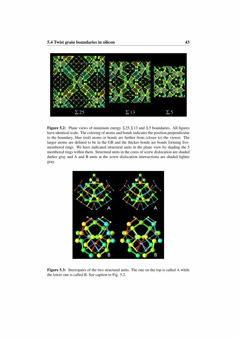
5.4 Twist grain boundaries in silicon 43
Figure 5.2: Plane views of minimum energy 625,613 and 65 boundaries. All figureshave identical scale. The coloring of atoms and bonds indicates the position perpendicularto the boundary, blue (red) atoms or bonds are further from (closer to) the viewer. Thelarger atoms are defined to be in the GB and the thicker bonds are bonds forming five-membered rings. We have indicated structural units in the plane view by shading the 5membered rings within them. Structural units in the cores of screw dislocation are shadeddarker gray and A and B units at the screw dislocation intersections are shaded lightergray.
A A
B B
Figure 5.3: Stereopairs of the two structural units. The one on the top is called A whilethe lower one is called B. See caption to Fig. 5.2.

44 Overview of the results
Figure 5.4: Plane views of minimum energy 617 and 629 boundaries. The figures haveidentical scale to the ones in Fig. 5.2. See caption to Fig. 5.2

5.4 Twist grain boundaries in silicon 45
Figure 5.5: 65 boundaries where each computational supercell contained 2×2 primitivecells in the GB plane. In each case the number of atoms removed per primitive cell is1N = 7. The boundary energies are 1069, 1091, 1095 and 1121 mJ/m2 for the top left,top right, bottom left and bottom right configurations, respectively. The size of the 2 × 2supercell is indicated by a white dashed box. Bonds in five-membered rings are shownto highlight the structural units. See caption to Fig. 5.2. Reprinted with permission fromPublication V. Copyright (2006) by the American Physical Society.

46 Overview of the results
∆
N=22
N=23 N=24
N=21∆ ∆
∆
Figure 5.6: 613 boundaries where each simulation supercell contained 2 × 2 primitivecells in the GB plane. In each case the value of 1N signifies the number of atoms removedper primitive cell. The size of the supercell is indicated by white dashed boxes. Bondsin five-membered rings are shown to highlight the structural units. See caption to Fig.5.2. Reprinted with permission from Publication V. Copyright (2006) by the AmericanPhysical Society.

Chapter 6
Summary
In this thesis the structure and kinetics of a number of silicon and silica systemshave been studied with computer simulations. The author has developed inde-pendently all simulational and analysis tools used in these studies. This has beenvital in order to find novel ways to simulate, and in particular analyze the studiedsystems. The research itself has been published in five publications, all of whichare included in this compilation. The main results of this thesis are as follows.First, new potential model parameters which can be used for creating realisticamorphous silica have been developed. Second, the collapse of an amorphouscluster embedded in crystalline silicon has been modeled. The methodology canalso be used for other materials more relevant to phase change memory devices.Third, new ordered structures have been found for twist grain boundaries in sil-icon by considering all possible atomic densities at the boundary. In addition toorder, structural units were also found. These formed a number of boundaries asis predicted by the structural unit model. This is perhaps the most significant con-tribution in this thesis as the question whether high-angle twist grain boundariesare formed of amorphous intergranular films has been an actively disputed topicin the grain boundary community.
The next topic of research also concerns grain boundaries. Now that orderedlow energy grain boundary structures at 0 K have been calculated, the focus willchange to their properties at finite temperatures. When grain boundaries areheated, the boundary undergoes a melting transition at temperatures lower thanthe bulk melting temperature. The preliminary results show that this is a con-tinuous transition. They also show that the structural units are very stable. Attemperatures up to 80% of the melting temperature the network of structural unitsin 625,613 and 65 is stable, but visits also the higher energy metastable statespresented in the case of 65. At temperatures above this, there are still metastablestructural units, even though most of the boundary has melted.

48 Summary

Appendix A
Atomicdx
The visualization package that the author has developed is named Atomicdx. Itcan visualize atoms and bonds, and also perform some simple analysis tasks. Themain goal has been to develop a tool with which one can perform a visual exam-ination of a series of atomistic systems (frames). This enables one to explore thesystem interactively and examine both its structure and the relationship betweendata associated with either atoms or bonds as a function of time. The structure ofa frame is studied by drawing a selected set of atoms and bonds. The selection canbe based on any atom or bond data. This enables one to draw only the interestingparts of a system. For example, in Publications IV and V the GB structure is eas-ier to grasp if the crystalline grains are not drawn. Data associated with atoms orbonds are visualized by either changing the coloring, or the sizes or shapes of thembased on the data. The data are usually scalar valued but for atoms one can alsohave vectorial data. Typical atom data are their potential, atom-type and velocitywhile typical bond data are the length of the bond, and atom data interpolated onthe bonds.
Atomicdx has been implemented using Opendx (www.opendx.org). Opendxis an opensource visualization package that can be used to create visualizations ofdifferent kinds of data. The visualization is built as a network of data processingmodules. The first module in the network imports data. The data are then passedon to modules which transform them in to a form that can be visualized. Thevisualization data are passed on to output modules which plot a graph, draw animage or write out data to a file. As Opendx has efficient data-caching only theparts of the network with changed input data will be executed. This allows evenvery large visualization networks to show good performance, but also means thatthe memory requirements can be relatively high. Atomicdx is built as such anetwork containing a number of custom modules to facilitate the loading of atomicsystems and calculating certain data values useful for analysis and visualization.The goal of Atomicdx was to create a visualization tool that can be used with

50 Atomicdx
Figure A.1: A typical session in Atomicdx. The main control panel allows one to openthe other control panels, images and colormaps and to choose which glyphs are visualized.Also a visualization and two data distributions is shown.
no prior knowledge of Opendx. Atomicdx can be operated with control panelshaving no need to touch the network itself. This hides the complexity of Opendxfrom the user but at the same time one can use the full power of Opendx within thecreated framework if needed. In Fig. A.1 an example of using Atomicdx is givenshowing two control panels and a visualization together with some statistics.
One can load atomistic systems into Atomicdx by reading in files which givethe positions of the atoms and optionally also two scalars, a data vector, and bond-ing information. If there is no bonding information Atomicdx can calculate it us-ing the cell-method (Frenkel et al., 2001). After the frames have been successfullyloaded one can calculate new data for the bonds and atoms. These data are alwayscalculated only for the active frame, not all frames. Change data are vectorialdata associated with the atoms that measure the distance the atoms have movedbetween frames. If the number of atoms is different this is calculated only forthe atoms that are in both frames. The identity of an atom is given by its indexnumber, i.e. the order in which it appears in the input. It is useful for findingchanges in structure between frames and also for looking at diffusion. One canalso clusterize data and calculate a cluster data component. A cluster consists ofa contiguous set of atoms which have a datavalue within a certain interval. Infigure A.2 an example of clusterization is given. In the figure Si atoms have beenclusterized by clusterizing the type data. One can also calculate datadistance data.These data allow us to classify atoms based on their distance from a set of atoms.The distance value for each atom is defined as the minimum number of bondsone has to traverse to get to the selected set. In figure A.2 an example of thedatadistance is given. There the set of atoms from which the distance is calcu-lated are the ones which form the previously mentioned clusters. Finally one canalso calculate an atom dependent custom data component by writing an arithmeticexpression involving any of the other data components.
The visualization capabilities in more detail are the following. Data are used

51
Figure A.2: Three visualization of a 2D-model of SiO illustrating the clusterization anddata distance. On the left: Colors represent the type of atom. Center: Colors representclusters of Si. Only the two largest ones are shown. On the right: Colors represent thedatadistance from the clusters. Only the first four layers are drawn.
to set the color, size and shape of glyphs representing atoms and bonds. Thecoloring can also be affected by changing the color maps which map data valuesto colors. The glyph type depends on the chosen glyph data. Bonds are alwaysdrawn as tubes connecting the atoms. Atoms are drawn as spheres when the glyph-data are scalar and as arrows when the glyph data are vectorial. The radius of thesphere is proportional to the scalar value, and the arrow is in the direction of thevector with a length proportional to the length of the vector. One can changethe amount of detail in the spheres and bonds to either produce output qualityimages by increasing it, or to produce fast visualizations with a fast refresh rateby decreasing it. The visualized system can be arbitrarily and interactively rotatedand moved. It is also easy to zoom in on the interesting parts.
In the program one can analyze atom and bond data. Only the atoms and bondsselected to be shown in the visualization are included in the analysis, and the datathat are analyzed are the one used for coloring. For both the atom and bonddata one can calculate a histogram and other basic statistics such as minimum,maximum, mean and variance. One can also plot the atom data with respect toanother user defined data as a scatter or line plot. In the line plot the value ofthe line is given by the mean, standard deviation, maximum or minimum of thecoloring data. Other statistics include the bond-angle distribution and the radialdistribution function.

52 Atomicdx

References
Allen, M. P. and Tildesley, D. J. (1987). Computer simulation of liquids. Clarendon Press,New York, NY, USA.
Andersen, H. C. (1980). Molecular dynamics at constant pressure and/or temperature.Journal of Chemical Physics, 72:2384.
Ashcroft, N. W. and Mermin, N. D. (1976). Solid State Physics. Saunder Collage Pub-lishing.
Balamane, H., Halicioglu, T., and Tiller, W. (1992). Comparative study of silicon empiri-cal interatomic potentials. Physical Review B, 46:2250.
Barkema, G. and Mousseau, N. (2000). High-quality continuous random networks. Phys-ical Review B, 62:4985.
Berendsen, H. J. C., Postma, J. P. M., van Gunsteren, W. F., DiNola, A., and Haak,J. R. (1984). Molecular dynamics with coupling to an external bath. J. Chem. Phys.,81(8):3684–3690.
Brotherton, S. D. (1995). Polycrystalline silicon thin film transistors. Semicond. Sci.Technol., 10:721–738.
Burlakov, V. M., Briggs, G. A. D., Sutton, A. P., and Tsukahara, Y. (2001). Monte carlosimulation of growth of porous SiOx by vapor deposition. Physical Review Letters,86:3052.
Chan, S. L. and Elliot, S. R. (1992). Calculation of diffusion activation energies in co-valent solids: application to vitreous silica. Journal of Physics: Condensed Matter,4:1269.
Cleri, F., Keblinski, P., Colombo, L., Phillpot, S. R., and Wolf, D. (1998). Correlationbetween atomic structure and localized gap states in silicon grain boundaries. Phys.Rev. B, 57:6247.
Cook, S. J. and Clancy, P. (1993). Comparison of semi-empirical potential functions forsilicon and germanium. Phys. Rev. B, 47(13):7686–7699.
D’Anterroches, C. and Bourret, A. (1984). Atomic structure of (011) and (001) near-coincident tilt boundaries in germanium and silicon. Phil. Mag. A, 49:783.

54 References
Feldman, J. L., Kluge, M. D., Allen, P. B., and Wooten, F. (1993). Thermal conductivityand localization in glasses: Numerical study of a model of amorphous silicon. Phys.Rev. B, 48(17):12589–12602.
Frenkel, D., Frenkel, D., and Smit, B. (2001). Understanding Molecular Simulation.Academic Press, Inc., Orlando, FL, USA.
Gibson, J. B., Goland, A. N., Milgram, M., and Vineyard, G. H. (1960). Dynamics ofradiation damage. Phys. Rev., 120(4):1229–1253.
Grovenor, C. R. M. (1985). Grain boundaries in semiconductors. J. Phys. C: Solid StatePhys., 18:4079–4119.
Hedler, A., Klaumünzer, S. L., and Wesch, W. (2004). Amorphous silicon exhibits a glasstransition. Nature mat., 3:804.
Howe, J. M. (1997). Interfaces in Materials. John wiley sons, inc.
Justo, J. F., Bazant, M. Z., Kaxiras, E., Bulatov, V. V., and Yip, S. (1998). Interatomicpotentials for silicon defects and disordered phases. Physical Review B, 58:2539.
Keating, P. (1966). Effect of invariance requirements on the elastic strain energy of crys-tals with application to the diamond structure. Physical Review, 145:637.
Keblinski, P., Phillpot, S. R., and Wolf, D. (1997). On the thermodynamic stability ofamorphous intergranular films in covalent materials. J. Am. Ceram. Soc., 80:177.
Keblinski, P., Phillpot, S. R., Wolf, D., and Gleiter, H. (1996). Thermodynamic criterionfor the stability of amorphous intergranular films in covalent materials. Phys. Rev. Lett.,77:2965.
Keskar, N. R. and Chelikowsky, J. R. (1992). Structural properties of nine silica poly-morphs. Physical Review B, 46:1.
Kleinman, D. A. and Spitzer, W. G. (1962). Theory of the optical properties of quartz inthe infrared. Phys. Rev., 125(1):16–30.
Kohyama, M. and Yamamoto, R. (1994). Tight-binding study of grain boundaries in Si:Energies and atomic structures of twist grain boundaries. Phys. Rev. B., 49:17102.
Kohyama, M., Yamamoto, R., Ebata, Y., and Kinoshita, M. (1988). The atomic andelectronic structure of a <001> tilt grain boundary in Si. J. Phys. C: Solid State Phys.,21:3205.
Mauri, F., Pasquarello, A., Pfrommer, B. G., Yoon, Y.-G., and Louie, S. G. (2000). Si-O-Si bond-angle distribution in vitreous silica from first principles Si NMR analysis.Phys. Rev. B, 62:4786.
Metropolis, N., Rosenbluth, A. W., Rosenbluth, M. N., Teller, A. H., and Teller, E. (1953).Equation of state calculations by fast computing machines. The Journal of ChemicalPhysics, 21(6):1087–1092.
References 55
Morigaki, K. (1999). Physics of Amorphous Semiconductors. Imperial College Press.
Mozzi, R. L. and Warren, B. E. (1969). The structure of vitrous silica. J. Appl. Crystal-logr., 2:164.
Nosé, S. (1984). A unified formulation of the constant temperature molecular dynamicsmethod. J. Chem. Phys., 81:511.
Otsuki, A. (2001). Misorientation dependence of energies of Si(001) twist grain bound-aries. Interf. Sci., 9:293.
Payne, M. C., Bristowe, P. D., and Joannopoulos, J. D. (1987). Ab initio determination ofthe structure of a grain boundary by simulated quenching. Phys. Rev. Lett., 58:1348.
Press, W. H., Teukolsky, S. A., Wtterling, W. T., and Flannery, B. P. (1995). NumericalRecipies in C. Cambridge University Press.
Read, W. T. and Shockley, W. (1950). Dislocation models of crystal grain boundaries.Phys. Rev., 78:275.
Rino, J. P., Ebbsjö, I., Kalia, R. K., Nakano, A., and Vashishta, P. (1993). Structure ofrings in vitreous SiO2. Physical Review B, 47(6):3053.
Ruault, M. O., Chaumont, J., Penisson, J. M., and Burret, A. (1984). High resolution andin situ investigation of defects in Bi-irradiated Si. Phil. Mag. A, 50:667–675.
Shanks, H. R., Maycock, P. D., Sidles, P. H., and Danielson, G. C. (1963). Thermalconductivity of silicon from 300 to 1400◦K. Phys. Rev., 130(5):1743–1748.
Stillinger, F. H. and Weber, T. A. (1985). Computer simulation of local order in condensedphases of silicon. Phys. Rev. B, 31:5262.
Streitz, F. H., Glosli, J. N., and Patel, M. V. (2006). Beyond finite-size scaling in solidifi-cation simulations. Phys. Rev. Lett., 96(22):225701.
Susman, S., Volin, K. J., Montague, D., and Price, D. L. (1991a). Temperature dependanceof the first sharp diffraction peak in vitreous silica. Phys. Rev. B, 43:11076.
Susman, S., Volin, K. J., Price, D. L., Grimsditch, M., Rino, J. P., and Kalia, R. K.(1991b). Intermediate-range order in permanently densified vitrous SiO2: A neutrondiffraction and molecular dynamics study. Phys. Rev. B, 43:1194.
Sutton, A. (1991). Grain boundaries in elemental and compound semiconductors. InWerner, J. and Strunk, H., editors, Polycrystalline Seiconductors II, Springer Proc.Phys., page 116. Springer-verlag: Berlin.
Sutton, A. P. and Balluffi, R. W. (1995). Interfaces in crystalline materials. OxfordUniversity Press, New York.
Sutton, A. P. and Vitek, V. (1983). On the structure of tilt grain boundaries in cubic metals.I. Symmetrical tilt boundaries. Phil. Trans. Soc. Lond. A, 309:1.

56 References
Tarnow, E., Dallot, P., Bristowe, P. D., Joannopoulos, J. D., Francis, G. P., and Payne,M. C. (1990). Structural complexity in grain boundaries with covalent bonding. Phys.Rev. B, 42:3644.
ten Wolde, P. R., Ruiz-Montero, M. J., and Frenkel, D. (1995). Numerical evidence forbcc ordering at the surface of a critical fcc nucleus. Phys. Rev. Lett., 75:2714.
Tersoff, J. (1986). New empirical model for the structural properties of silicon. PhysicalReview Letters, 56:632.
Tersoff, J. (1988a). Empirical interatomic potential for silicon with improved elastic prop-erties. Phys. Rev. B, 38:9902.
Tersoff, J. (1988b). New empirical approach for the structure and energy of covalentsystems. Physical Review B, 37:6991.
Tsuneyuki, S., Tsukada, M., Aoki, H., and Matsui, Y. (1988). First-principles interatomicpotential of silica applied to molecular dynamics. Phys. Rev. Lett., 61(7):869–872.
Tu, Y. and Tersoff, J. (2000). Structure and energetics of the Si-SiO2 interface. PhysicalReview Letters, 84(19):4393.
Tu, Y., Tersoff, J., and Grinstein, G. (1998). Properties of continuous-random-networkmodel for amorphous systems. Physical Review Letters, 81:4899.
Uchino, T., Kitagawa, Y., and Yoko, T. (2000). Structure, energies and vibrational prop-erties of silica rings in SiO2 glass. Phys. Rev. B, 61:234.
van Beest, B. W. H., Kramer, G. J., and van Santen, R. A. (1990). Force fields for silicasand aluminophosphates based on ab initio calculations. Phys. Rev. Lett., 64(16):1955–1958.
van Laarhoven, P. J. M. and Aarts, E. H. L. (1987). Simulated Annealing: Theory andApplications. D. Reidel Publishing Company.
Vashishta, P., Kalia, R. K., Rino, J. P., and Ebbsjö, I. (1990). Interaction potential for sio2:A molecular-dynamics study of structural correlations. Phys. Rev. B, 41(17):12197–12209.
Vink, R., Barkema, G., van der Weg, W., and Mousseau, N. (2001). Fitting the Stillinger-Weber potential to amorphous silicon. Journal of non-crystalline solids, 282:248.
Wang, Z. Q., Dregia, S. A., and Stroud, D. (1994). Energy-minimization studies of twistgrain boundaries in diamond. Phys. Rev. B., 49:8206.
Wooten, F., Winer, K., and Weaire, D. (1985). Computer generation of structural modelsof amorphous Si and Ge. Physical Review Letters, 54:1392.